Visualization Research - faculty.cs.niu.edu

Information Visualization

Visualization Research

Dr. David Koop

D. Koop, CSCI 628, Fall 2021

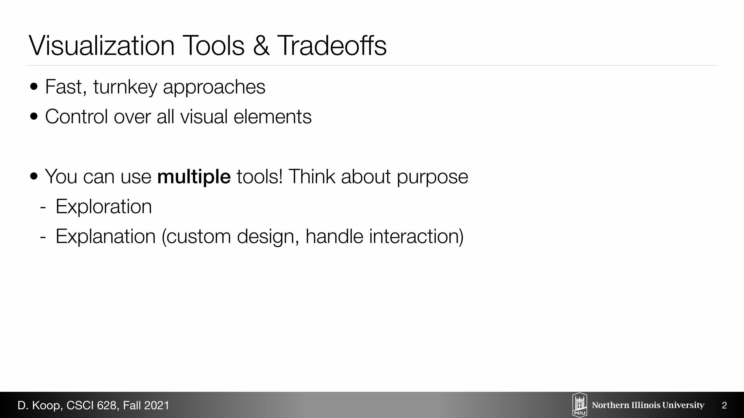
Visualization Tools & Tradeoffs• Fast, turnkey approaches • Control over all visual elements

• You can use multiple tools! Think about purpose - Exploration - Explanation (custom design, handle interaction)

2D. Koop, CSCI 628, Fall 2021

Scatterplot Matrices and Parallel Coordinates

3

[Munzner (ill. Maguire), 2014]D. Koop, CSCI 628, Fall 2021

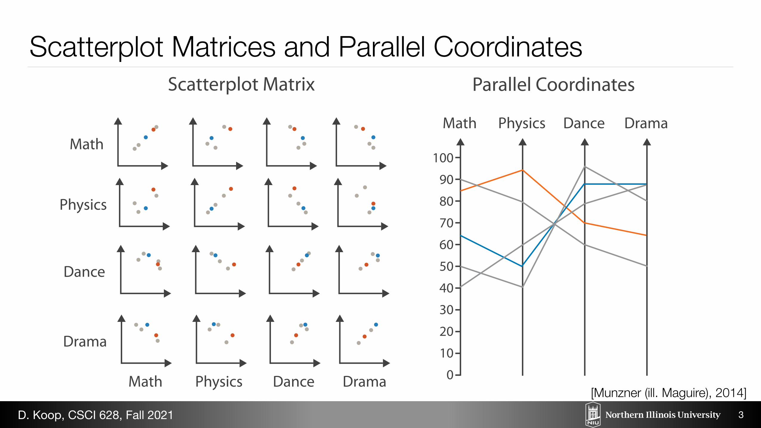
Math

Physics

Dance

Drama

Math Physics Dance Drama


1009080706050 40302010

0


8590655040

9580504060

7060909580

6550908090

Table Scatterplot Matrix Parallel Coordinates

Scatterplot Matrices and Parallel Coordinates

3


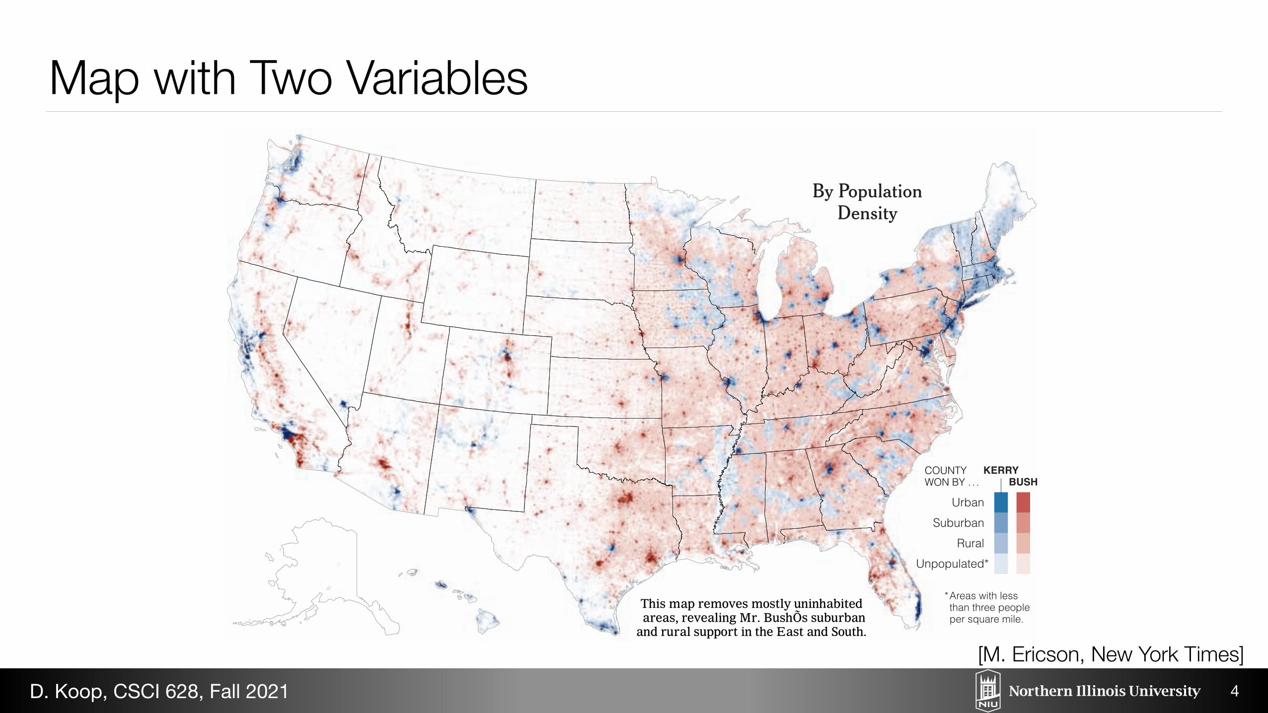
By Population Density

Areas with less than three people per square mile.

*

COUNTYWON BY . . .

Urban

Suburban

Rural

Unpopulated*

BUSHKERRY

6JKU�OCR�TGOQXGU�OQUVN[�WPKPJCDKVGF�CTGCU��TGXGCNKPI�/T��$WUJ�U�UWDWTDCP�

CPF�TWTCN�UWRRQTV�KP�VJG�'CUV�CPF�5QWVJ��

Map with Two Variables

4

[M. Ericson, New York Times]D. Koop, CSCI 628, Fall 2021

NodeLinkTreeLayout12,870

RadialTreeLayout12,348

CirclePackingLayout12,003

CircleLayout9,317

TreeMapLayout9,191

StackedAreaLayout9,121

ForceDirectedLayout8,411

Layout7,881

AxisLayout6,725

IcicleTreeLayout4,864

DendrogramLayout4,853

BundledEdgeRouter3,727

IndentedTreeLayout3,174PieLayout2,728

RandomLayout870

Labeler9,956

RadialLabeler3,899

StackedAreaLabeler3,202

PropertyEncoder4,138

Encoder4,060

ColorEncoder3,179

SizeEncoder1,830

ShapeEncoder

Distortion6,314

BifocalDistortion4,461

FisheyeDistortion3,444

FisheyeTreeFilter5,219

VisibilityFilter3,509

GraphDistanceFilter3,165

OperatorList5,248

OperatorSequence4,190

OperatorSwitch2,581

Operator2,490

SortOperator2,023

IOperator1,286

Data20,544

DataList19,788

NodeSprite19,382

ScaleBinding11,275

DataSprite10,349

TreeBuilder9,930

EdgeRenderer5,569

ShapeRenderer2,247

ArrowType698IRenderer

Tree7,147

EdgeSprite3,301

TooltipControl8,435

SelectionControl7,862

PanZoomControl5,222

HoverControl4,896

ControlList4,665

ClickControl3,824

ExpandControl2,832

DragControl2,649

AnchorControl2,138

Control1,353

IControl763

Legend20,859

LegendRange10,530

LegendItem4,614

Axis24,593

CartesianAxes6,703

Axes1,302

AxisGridLineAxisLabel

Visualization16,540

DataEvent2,313SelectionEvent1,880

TooltipEvent1,701VisualizationEvent1,117Strings

22,026

Shapes19,118

Maths17,705

Displays12,555

ColorPalette6,367

SizePalette2,291

ShapePalette2,059

Palette1,229

Geometry10,993

FibonacciHeap9,354

HeapNode1,233

Colors10,001

SparseMatrix3,366

DenseMatrix3,165

IMatrix2,815

Arrays8,258

Dates8,217

Sort6,887

Stats6,557

Property5,559

Filter2,324

Orientation1,486

IValueProxy874IPredicate383

IEvaluable335

Interpolator8,746

MatrixInterpolator2,202

ColorInterpolator2,047

RectangleInterpolator2,042

ArrayInterpolator1,983

PointInterpolator1,675

ObjectInterpolator1,629

NumberInterpolator1,382

DateInterpolator

Transitioner19,975

Easing17,010

Transition9,201

Tween6,006

FunctionSequence5,842

Scheduler5,593

Sequence5,534

Parallel5,176

TransitionEvent1,116

ISchedulable1,041

Pause449

range772

iff748

gte625

lte619

gt603

mul603

sub600

neq599

lt597

div595

eq594

add593

mod591

isa461fn460notstddev

xor354

variance335

and330

or323

orderbyupdatewhereselect

distinct292average287max283

minsum

count277_264

Query13,896

Expression5,130

Comparison5,103

DateUtil4,141

StringUtil4,130

Arithmetic3,891

Match3,748

CompositeExpression3,677

ExpressionIterator3,617

Fn3,240

BinaryExpression2,893

If2,732

IsA2,039

Variance1,876

AggregateExpression1,616

Range1,594

Not1,554

Literal1,214Variable1,124

Xor1,101

And1,027

Or970

Distinct933Average891Maximum843

Minimum843

Sum791

Count781

MaxFlowMinCut7,840

ShortestPaths5,914

LinkDistance5,731

BetweennessCentrality3,534

SpanningTree3,416

HierarchicalCluster6,714

AgglomerativeCluster3,938CommunityStructure3,812

MergeEdge743

AspectRatioBanker7,074

TimeScale5,833

QuantitativeScale4,839

Scale4,268

OrdinalScale3,770

LogScale3,151

QuantileScale2,435

IScaleMap2,105

ScaleType1,821RootScale1,756

LinearScale1,316

GraphMLConverter9,800

DelimitedTextConverter4,294

JSONConverter2,220

IDataConverter1,314Converters721

DataSource3,331

DataUtil3,322

DataSchema2,165DataField

DataTable772DataSet

NBodyForce10,498

Simulation9,983

Particle2,822

Spring2,213

SpringForce1,681GravityForce

DragForce1,082

IForce

TextSprite10,066

DirtySprite8,833

RectSprite3,623

LineSprite1,732

FlareVis4,116

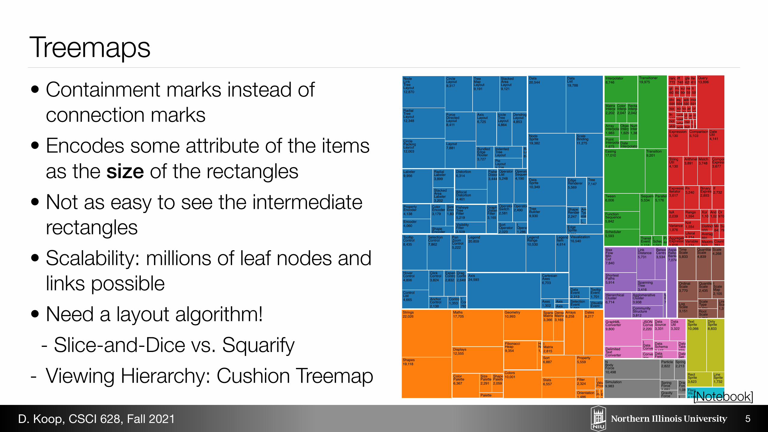
Treemaps• Containment marks instead of

connection marks • Encodes some attribute of the items

as the size of the rectangles • Not as easy to see the intermediate

rectangles • Scalability: millions of leaf nodes and

links possible • Need a layout algorithm! - Slice-and-Dice vs. Squarify

- Viewing Hierarchy: Cushion Treemap

5

[Notebook]D. Koop, CSCI 628, Fall 2021

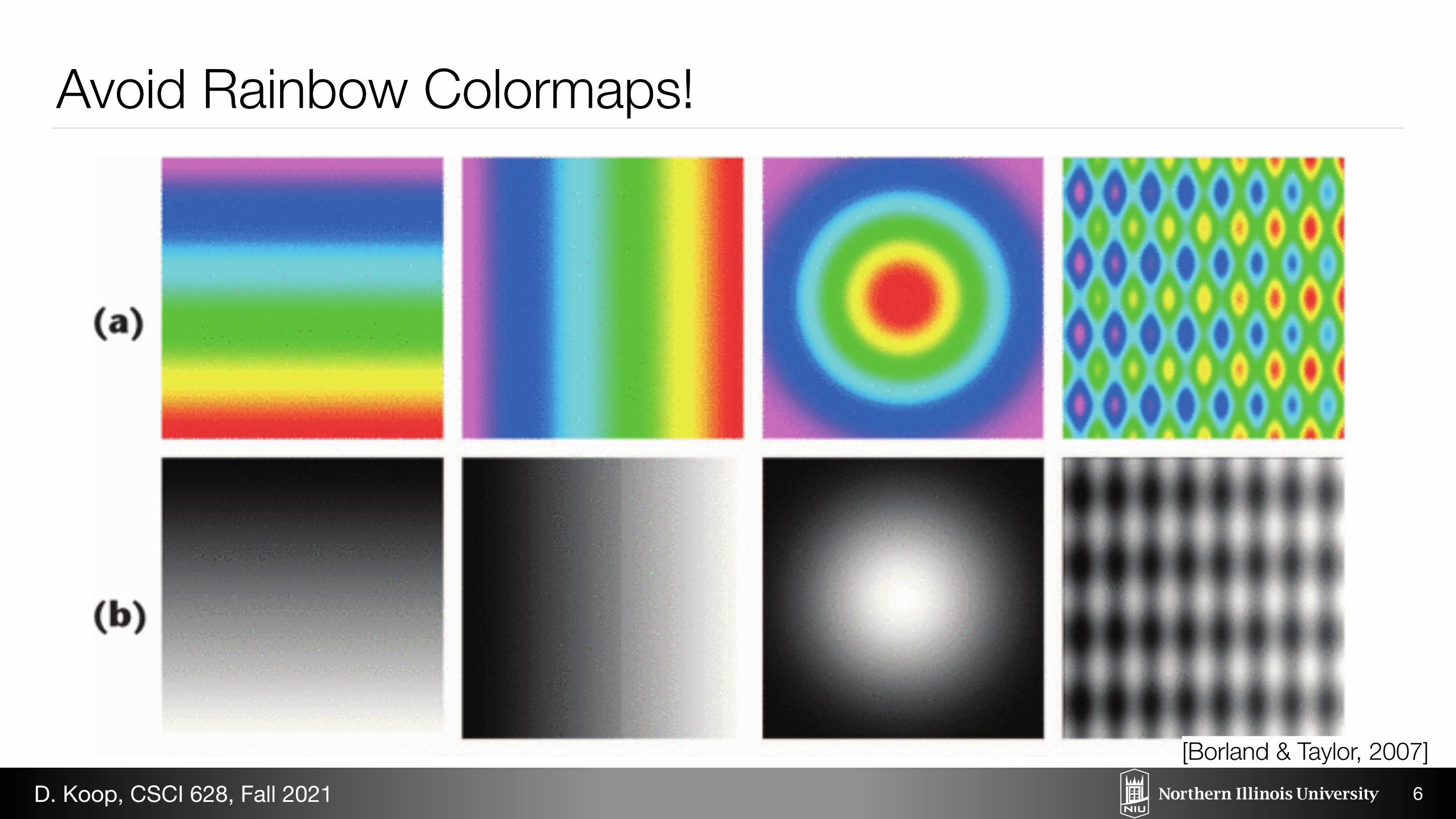
https://observablehq.com/@dakoop/treemap

Avoid Rainbow Colormaps!

6

[Borland & Taylor, 2007]D. Koop, CSCI 628, Fall 2021

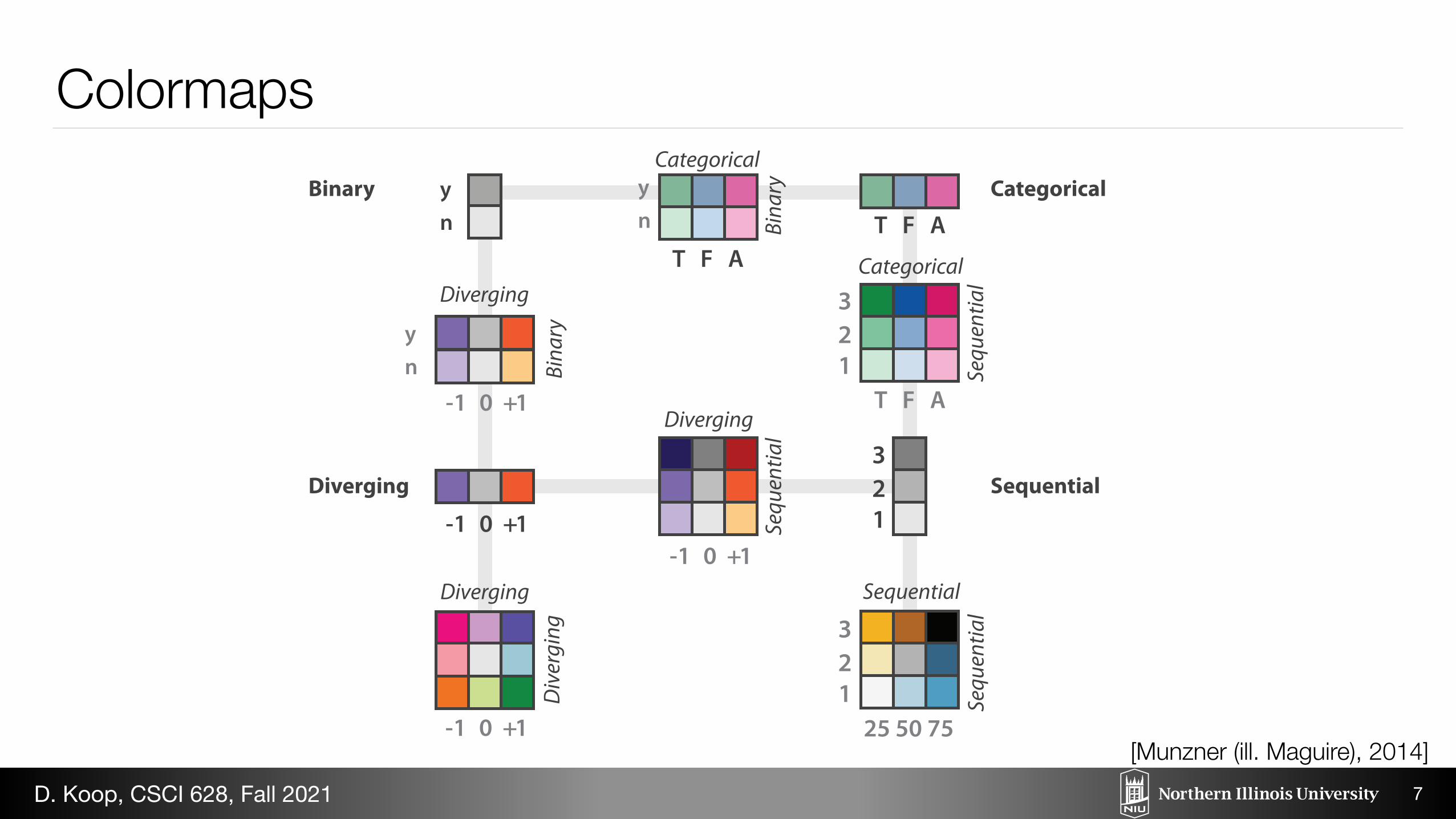
Binary

Diverging

Categorical

Sequential

Categorical

Categorical

Colormaps

7


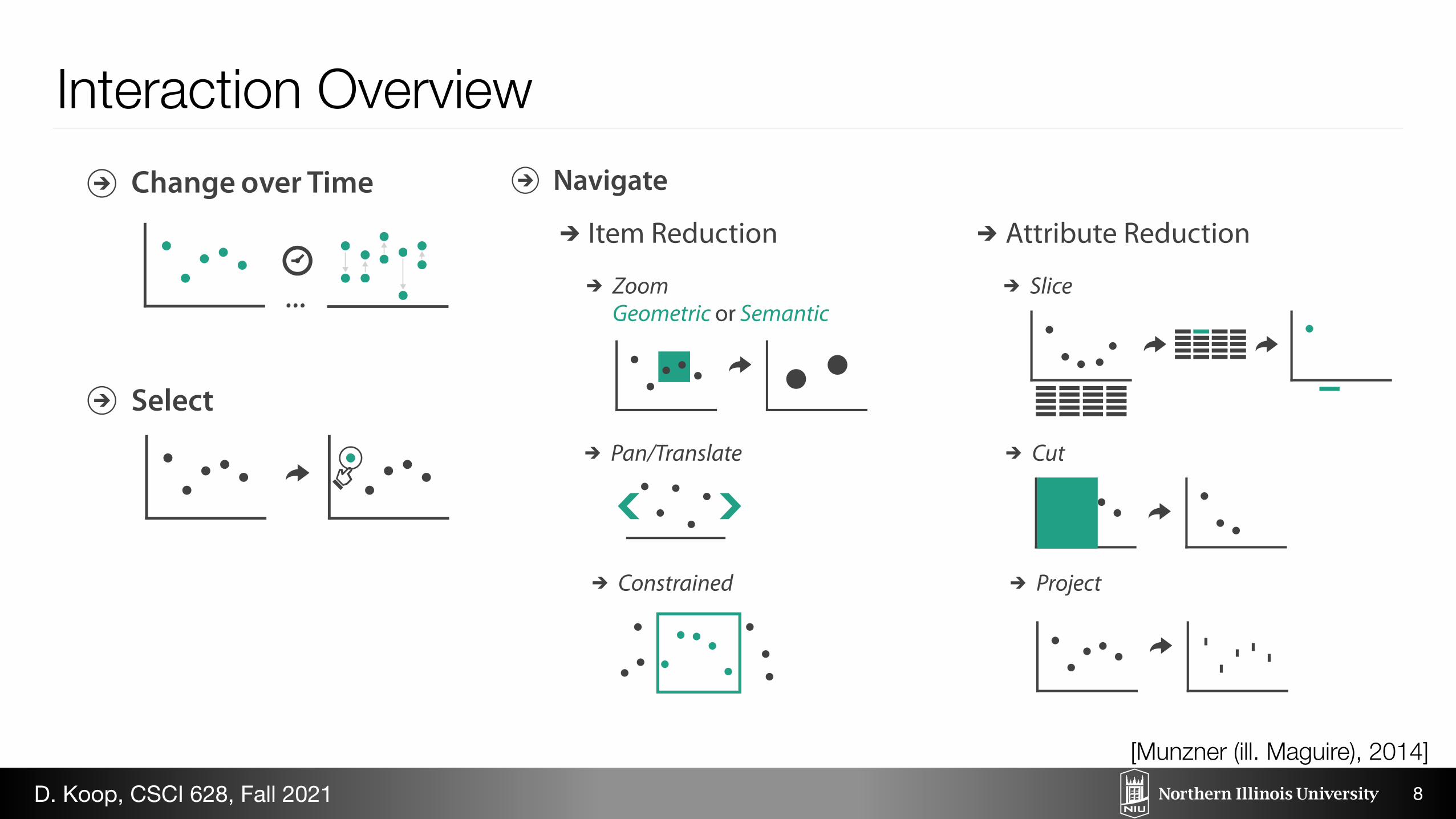
Manipulate

Change over Time

Select

Navigate

Item Reduction

Zoom

Pan/Translate

Constrained

Geometric or Semantic

Attribute Reduction

Slice

Cut

Project

Interaction Overview

8


Manipulate

Change over Time

Select

Navigate

Item Reduction

Zoom

Pan/Translate

Constrained

Geometric or Semantic

Attribute Reduction

Slice

Cut

Project

Animated Transitions

9

[M. Bostock]D. Koop, CSCI 628, Fall 2021

http://bl.ocks.org/mbostock/3943967

Animated Transitions

9



Facet

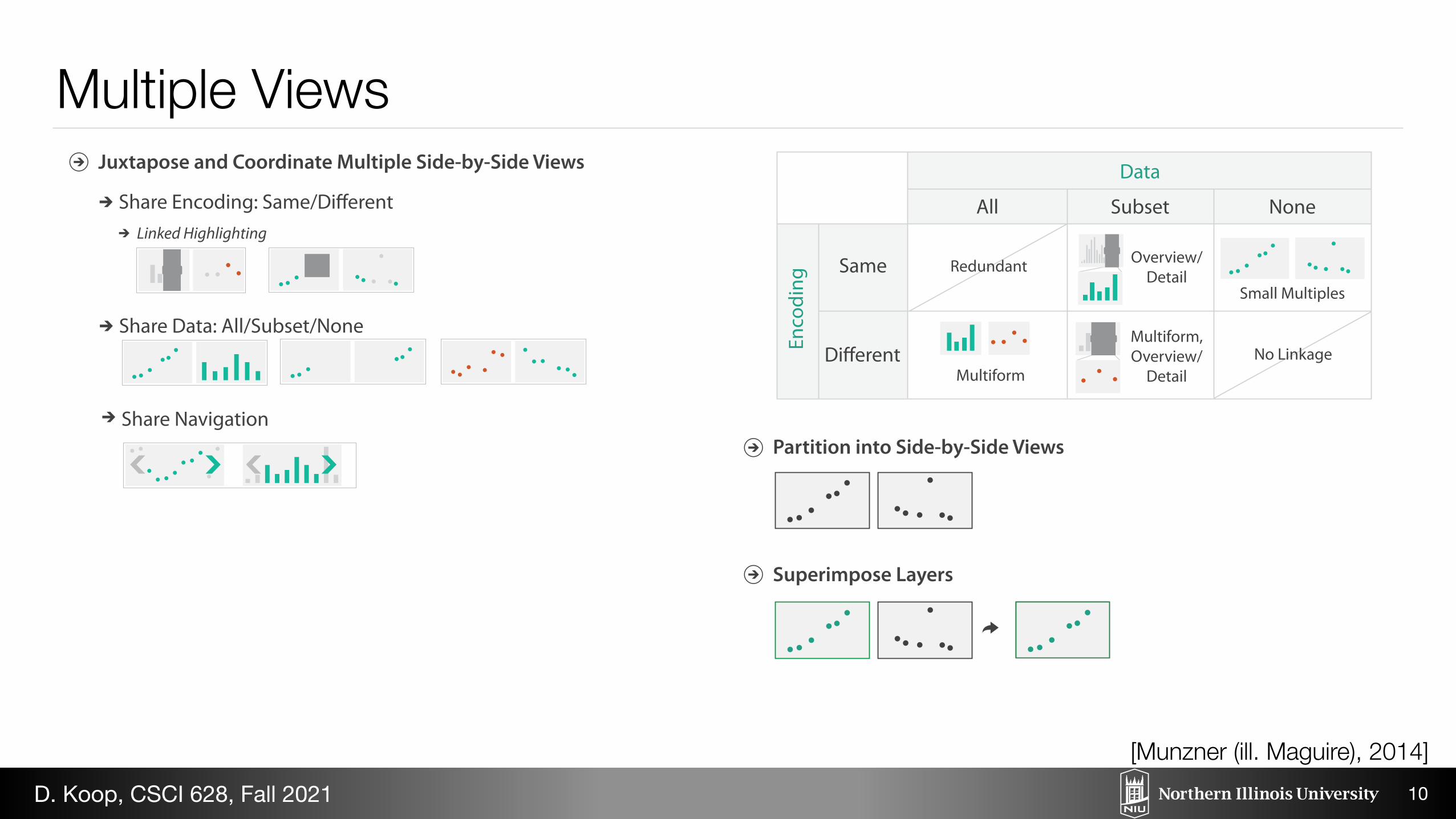
Partition into Side-by-Side Views

Superimpose Layers

Juxtapose and Coordinate Multiple Side-by-Side Views

Share Data: All/Subset/None

Share Navigation

All Subset

Same

Multiform

Multiform, Overview/

Detail

None

Redundant

No Linkage

Small Multiples

Overview/Detail

Linked Highlighting

Multiple Views

10

Facet

Partition into Side-by-Side Views

Superimpose Layers

Juxtapose and Coordinate Multiple Side-by-Side Views

Share Data: All/Subset/None

Share Navigation

All Subset

Same

Multiform

Multiform, Overview/

Detail

None

Redundant

No Linkage

Small Multiples

Overview/Detail

Linked Highlighting


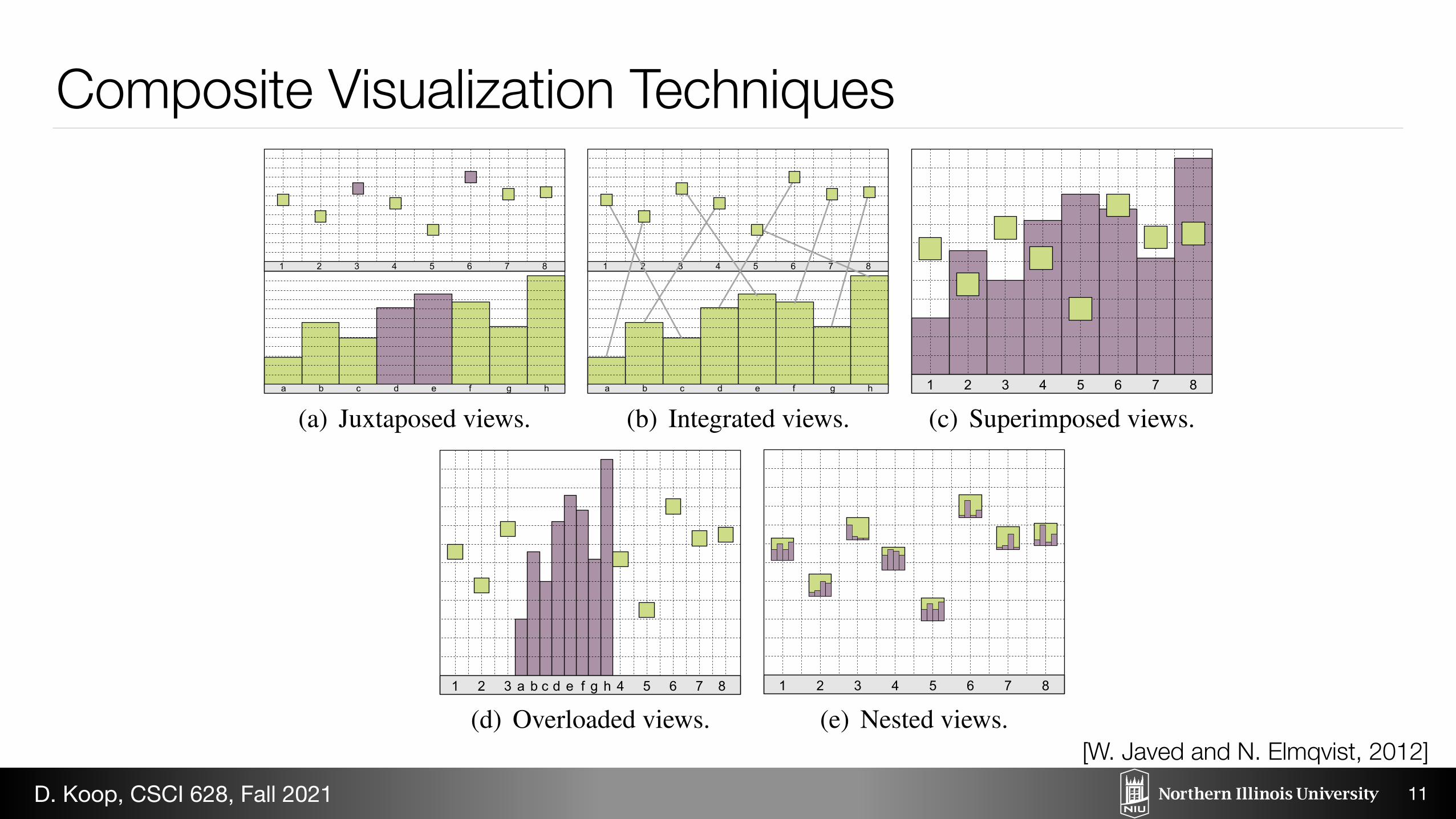
Composite Visualization Techniques

11

[W. Javed and N. Elmqvist, 2012]D. Koop, CSCI 628, Fall 2021

Technique Visualization A Visualization B Spatial Relation Data Relation

ComVis [24] (Figure 2) any any juxtapose noneImprovise [39] (Figure 3) any any juxtapose noneJigsaw [36] any any juxtapose noneSnap-Together [30] any any juxtapose nonesemantic substrates [34] (Figure 4) node-link node-link juxtapose item-itemVisLink [11] (Figure 5) radial graph node-link juxtapose item-itemNapoleon’s March on Moscow [37] time line view area visualization juxtapose item-itemMapgets [38] (Figure 6) map text superimpose item-itemGeoSpace [22] (Figure 7) map bar graph superimpose item-item3D GIS [8] map glyphs superimpose item-itemScatter Plots in Parallel Coordinates [45] (Figure 8) parallel coordinate scatterplot overload item-dimensionGraph links on treemaps [14] (Figure 9) treemap node-link overload item-itemSparkClouds [21] tag cloud line graph overload item-itemZAME [13] (Figure 10) matrix glyphs nested item-groupNodeTrix [17] (Figure 11) node-link matrix nested item-groupTimeMatrix [44] matrix glyphs nested item-groupGPUVis [25] Scatterplot glyphs nested item-group

Table 1: Classification of common composite visualization techniques using our design space.

(a) Juxtaposed views. (b) Integrated views. (c) Superimposed views. (d) Overloaded views. (e) Nested views.

Figure 12: Example of composing a scatterplot and bar graph using different methods.

datasets in the same space and using different visualizations, butalso highlights the relational linking between the two datasets.

Nested views provide an efficient approach to link each of thedata values, visualized through the host visualization, to its relateddataset, visualized through client visualizations. This is achievedby nesting clients inside the visual marks in the host.

• Benefits: Very compact representation, easy correlation.• Drawbacks: Limited space for the client visualizations, clut-

ter is high, and visual design dependencies are high.• Applications: Again, situations that call for augmenting a

particular visual representation with additional mapping.

Figure 12(e) shows an example composition of scatterplot andbar graph visualizations based on this design patter. In the figure,the scatterplot visualization is acting as a host and bar graph visu-alizations are nested inside its visual marks.

There is probably not a clear winner among different design pat-terns while designing an information visualization tool. The correctchoice of design pattern to use for a particular implementation de-pends on different conditions, such as the available view space, userknowledge, and the complexity of the underlying dataset. Ideallyspeaking, designers should be able to combine any existing visual-izations to generate a composite visualization view.

8.2 Delimitations

While our above CVV design patterns are general in nature, theyare based solely on the spatial layout of component visualizations.However, it is possible to envision other ways to combine two ormore visualizations, for example using interaction or animation.One such example is the use of interactive hyperlinking [6, 43] (orwormholing) to navigate between different visualization views.

8.3 Discussion

There are several direct benefits to structuring the design space ofcomposite visualization views in this manner. Classifying existingtechniques into patterns not only helps in understanding these tech-niques, but also in evaluating their strengths and weaknesses.

However, the design patterns presented in this paper are all basedon evidence from the literature of how existing visualization toolsand techniques use composite views. Therefore, our frameworkis inherently limited to current designs, and more descriptive thangenerative in nature. Furthermore, this list of patterns is not neces-sarily exhaustive, and we certainly foresee additional design pat-terns for composite views to emerge with progress in informa-tion visualization. It is also not always straightforward to sepa-rate what is a composite visualization and what is an “atomic” (orcomponent) visualization, particularly when the compositions onthe visual structures—which is the case for overloaded and nestedviews—as opposed to merely on the views. Our approach in theabove text has been to treat as components any technique has beenpresented in the literature as a standalone technique.

9 CONCLUSION

We have proposed a novel framework for specifying, designing, andevaluating compositions of multiple visualizations in the same vi-sual space that we call composite visualization views. The benefitof the framework is not only to provide a way to unify a large col-lection of existing work where visual representations are combinedin various ways, but also to suggest new combinations of visualrepresentations that may significantly advance the state of the art.

REFERENCES

[1] C. Ahlberg and B. Shneiderman. Visual information seeking: Tightcoupling of dynamic query filters with starfield displays. In Proceed-

Technique Visualization A Visualization B Spatial Relation Data Relation

ComVis [24] (Figure 2) any any juxtapose noneImprovise [39] (Figure 3) any any juxtapose noneJigsaw [36] any any juxtapose noneSnap-Together [30] any any juxtapose nonesemantic substrates [34] (Figure 4) node-link node-link juxtapose item-itemVisLink [11] (Figure 5) radial graph node-link juxtapose item-itemNapoleon’s March on Moscow [37] time line view area visualization juxtapose item-itemMapgets [38] (Figure 6) map text superimpose item-itemGeoSpace [22] (Figure 7) map bar graph superimpose item-item3D GIS [8] map glyphs superimpose item-itemScatter Plots in Parallel Coordinates [45] (Figure 8) parallel coordinate scatterplot overload item-dimensionGraph links on treemaps [14] (Figure 9) treemap node-link overload item-itemSparkClouds [21] tag cloud line graph overload item-itemZAME [13] (Figure 10) matrix glyphs nested item-groupNodeTrix [17] (Figure 11) node-link matrix nested item-groupTimeMatrix [44] matrix glyphs nested item-groupGPUVis [25] Scatterplot glyphs nested item-group

Table 1: Classification of common composite visualization techniques using our design space.

(a) Juxtaposed views. (b) Integrated views. (c) Superimposed views.1 2 3 4 5 6 7 8a b c d e f g h

(d) Overloaded views. (e) Nested views.

Figure 12: Example of composing a scatterplot and bar graph using different methods.

datasets in the same space and using different visualizations, butalso highlights the relational linking between the two datasets.

Nested views provide an efficient approach to link each of thedata values, visualized through the host visualization, to its relateddataset, visualized through client visualizations. This is achievedby nesting clients inside the visual marks in the host.

• Benefits: Very compact representation, easy correlation.• Drawbacks: Limited space for the client visualizations, clut-

ter is high, and visual design dependencies are high.• Applications: Again, situations that call for augmenting a

particular visual representation with additional mapping.

Figure 12(e) shows an example composition of scatterplot andbar graph visualizations based on this design patter. In the figure,the scatterplot visualization is acting as a host and bar graph visu-alizations are nested inside its visual marks.

There is probably not a clear winner among different design pat-terns while designing an information visualization tool. The correctchoice of design pattern to use for a particular implementation de-pends on different conditions, such as the available view space, userknowledge, and the complexity of the underlying dataset. Ideallyspeaking, designers should be able to combine any existing visual-izations to generate a composite visualization view.

8.2 Delimitations

While our above CVV design patterns are general in nature, theyare based solely on the spatial layout of component visualizations.However, it is possible to envision other ways to combine two ormore visualizations, for example using interaction or animation.One such example is the use of interactive hyperlinking [6, 43] (orwormholing) to navigate between different visualization views.

8.3 Discussion

There are several direct benefits to structuring the design space ofcomposite visualization views in this manner. Classifying existingtechniques into patterns not only helps in understanding these tech-niques, but also in evaluating their strengths and weaknesses.

However, the design patterns presented in this paper are all basedon evidence from the literature of how existing visualization toolsand techniques use composite views. Therefore, our frameworkis inherently limited to current designs, and more descriptive thangenerative in nature. Furthermore, this list of patterns is not neces-sarily exhaustive, and we certainly foresee additional design pat-terns for composite views to emerge with progress in informa-tion visualization. It is also not always straightforward to sepa-rate what is a composite visualization and what is an “atomic” (orcomponent) visualization, particularly when the compositions onthe visual structures—which is the case for overloaded and nestedviews—as opposed to merely on the views. Our approach in theabove text has been to treat as components any technique has beenpresented in the literature as a standalone technique.

9 CONCLUSION

We have proposed a novel framework for specifying, designing, andevaluating compositions of multiple visualizations in the same vi-sual space that we call composite visualization views. The benefitof the framework is not only to provide a way to unify a large col-lection of existing work where visual representations are combinedin various ways, but also to suggest new combinations of visualrepresentations that may significantly advance the state of the art.

REFERENCES

[1] C. Ahlberg and B. Shneiderman. Visual information seeking: Tightcoupling of dynamic query filters with starfield displays. In Proceed-

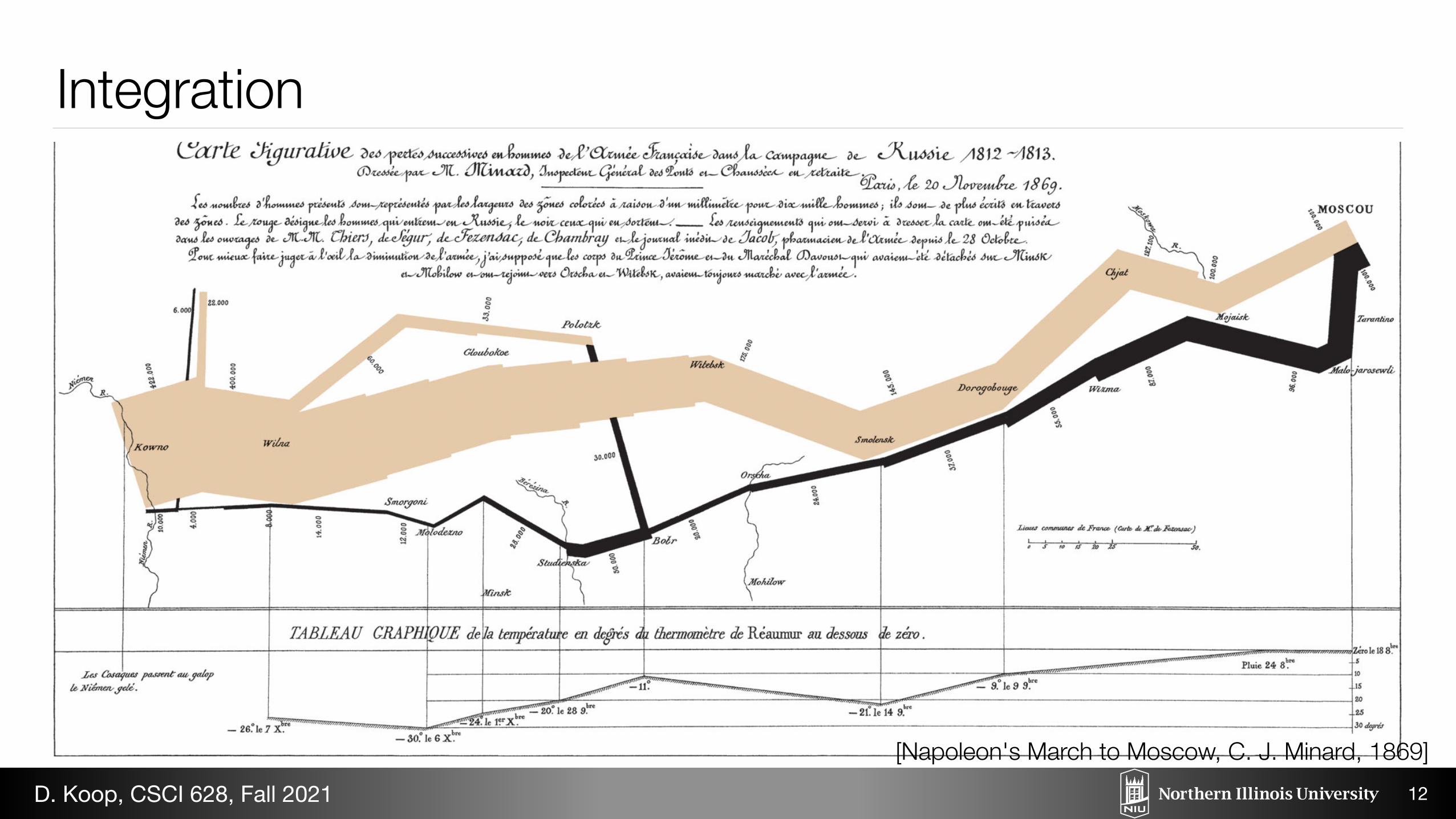
Integration

12

[Napoleon's March to Moscow, C. J. Minard, 1869]D. Koop, CSCI 628, Fall 2021

6 OVERLOADING ! OVERLOADED VIEWS

This design pattern characterizes compositions where one visual-ization, called the client visualization, is rendered inside anothervisualization, called the host, using the same spatial mapping as thehost [26]. Overloaded views (Figures 8 and 9) are similar to super-imposed views, but with some important differences. Like super-imposition, the client visualization in this design pattern is overlaidon the host. However, unlike Superimposed Views, there exists noone-to-one spatial linking between the two visualizations [12].

While previous design patterns have all operated on specificviews of component visualizations, overloaded views (and also thenext pattern, Nested Views) operate on the visual structure them-selves. In other words, it is no longer possible to merely use vi-sual layout operations to organize the views together, but the vi-sual structures themselves must be modified to combine the com-ponents. We will see examples of this below.

Figure 10: ZAME [13] (Nested Views). Visual exploration of a

protein-protein interaction dataset in ZAME.

6.1 Scatter Plots in Parallel Coordinates (SPPC)

Yuan et al. [45] presented a system that allows overloading of 2Dscatterplots on a parallel coordinates visualization [18] (Figure 8).The technique is based on converting the space between pairs ofselected coordinate dimensions in a parallel coordinate plot intoscatterplots through multidimensional scaling [42]. The techniquetakes advantage of the fact that parallel coordinate plots do not re-ally use the space between the parallel dimensional axes, whichmeans that this space is open for being overloaded.

SPPC is also an example of combining two techniques to com-pensate for their individual shortcomings. Parallel coordinates areefficient for visualizing multiple dimensions in a compact 2D vi-sual representation. However, they make it hard to correlate trendsacross multiple dimensions due to their inherent visual clutter. Scat-terplots, on the other hand, provide an effective way of correlatingtrends in any dimension of a dataset [10]. Combining both tech-niques allows for sharing their advantages.

6.2 Graph Links on Treemaps

Fekete et al. [14] proposed a technique for rendering graphs using atreemap [20] with overloaded graph links. The idea is based on thefact that it is possible to decompose a graph into a tree structure anda set of remaining graph edges that are not included in the tree. Thisgraph decomposition allows for using a treemap to visualize the treestructure, and then overload links corresponding to the remaininggraph edges on the treemap visualization. Even though Fekete et al.

call this “overlaying”, the technique is an example of overloadingin our terminology because the graph links are not just a separatelayer on top of the treemap, but they are embedded into the visualstructure of the treemap and use the node positions as anchors.

Figure 9 shows the technique being used to visualize a website.Here, the directory structure, inherent in any website, is visualizedthrough an underlying treemap and external links are visualizedthrough overlaid edges. The overlaid edges are not straight lines,but are curved to highlight source and target locations. The edgesare curved more near the source, hence making it easy to visuallyrecognize the direction of the link. The tool also supports con-trolling the visibility of various edges to reduce visual clutter, andcoloring edges based on their attributes.

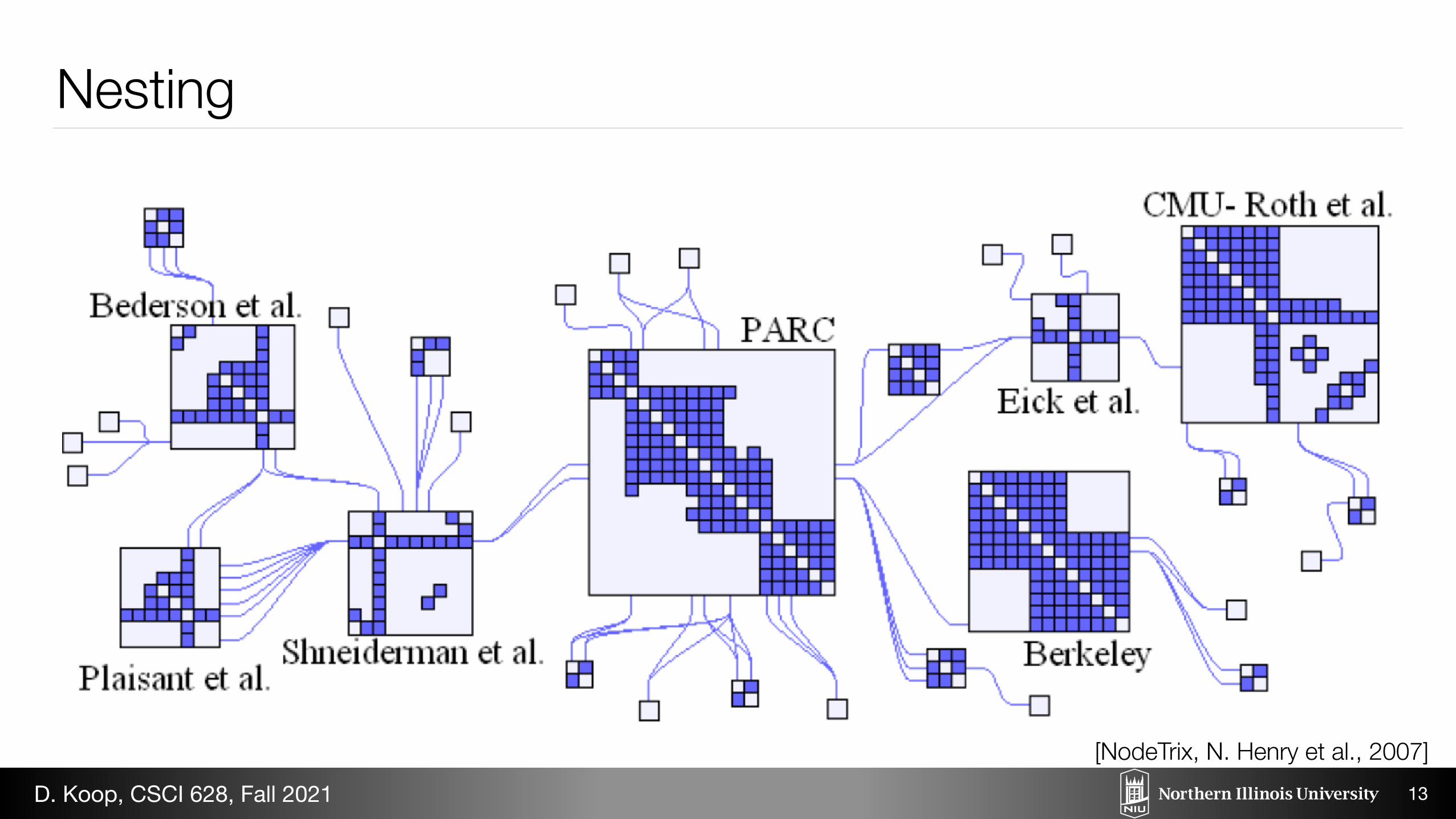
Figure 11: NodeTrix [17] (Nested Views). This example shows a

visualization of the InfoVis co-authorship network.

7 NESTING ! NESTED VIEWS

Nested views, like overloaded views, are also based on the notion ofhost and client visualizations. However, in this design pattern, oneor more client visualizations are nested inside the visual marks ofthe host visualizations, based on the relational linking between thepoints. Most often, the nesting is performed simply by replacingthe visual marks in the host visualization by nested instances of theclient visualization (Figures 10 and 11). An example of this wouldbe a scatterplot where the individual marks are barchart glyphs [25].

The nested views pattern provides an effective way of relatingdata points in the host visualization to the data visualized throughthe client visualizations. Again the users need not divide their atten-tion between multiple views, and the host visualization is allowedto use the full available space. However, since the design patternembeds one or more visualizations inside a visual mark, the clientvisualizations are allocated only a small portion of the host visual-ization’s visual space, and zooming and panning may be required tosee details. Furthermore, just like overloading, nested views com-pose the actual visual structures of the components, which typicallyrequires a more careful design.

One issue to discuss here is the difference between overloadingand nesting. These are different design patterns because nestingsimply replaces the visual marks of the host with the visual structureof the client, whereas overloading requires a much more integratedcomposition of the visual structures of the host and the client.

7.1 ZAME

Nested views are becoming increasingly prominent for visualizinglarge-scale datasets using glyph-based methods. ZAME [13], a vi-sualization system designed to explore large-scale adjacency matrixgraph visualization, uses this approach. The base matrix represen-tation used in ZAME is a hierarchical aggregation of the underly-ing dataset. The tool allows the user to zoom in data space, whichamounts to drilling-down and rolling-up in the aggregation hierar-chy to see more or less details. Abstract glyphs representing aggre-gated data for each cell in the matrix are nested inside the visualmarks of the matrix to convey information about the aggregation.

Nesting

13

[NodeTrix, N. Henry et al., 2007]D. Koop, CSCI 628, Fall 2021

Brushing

14



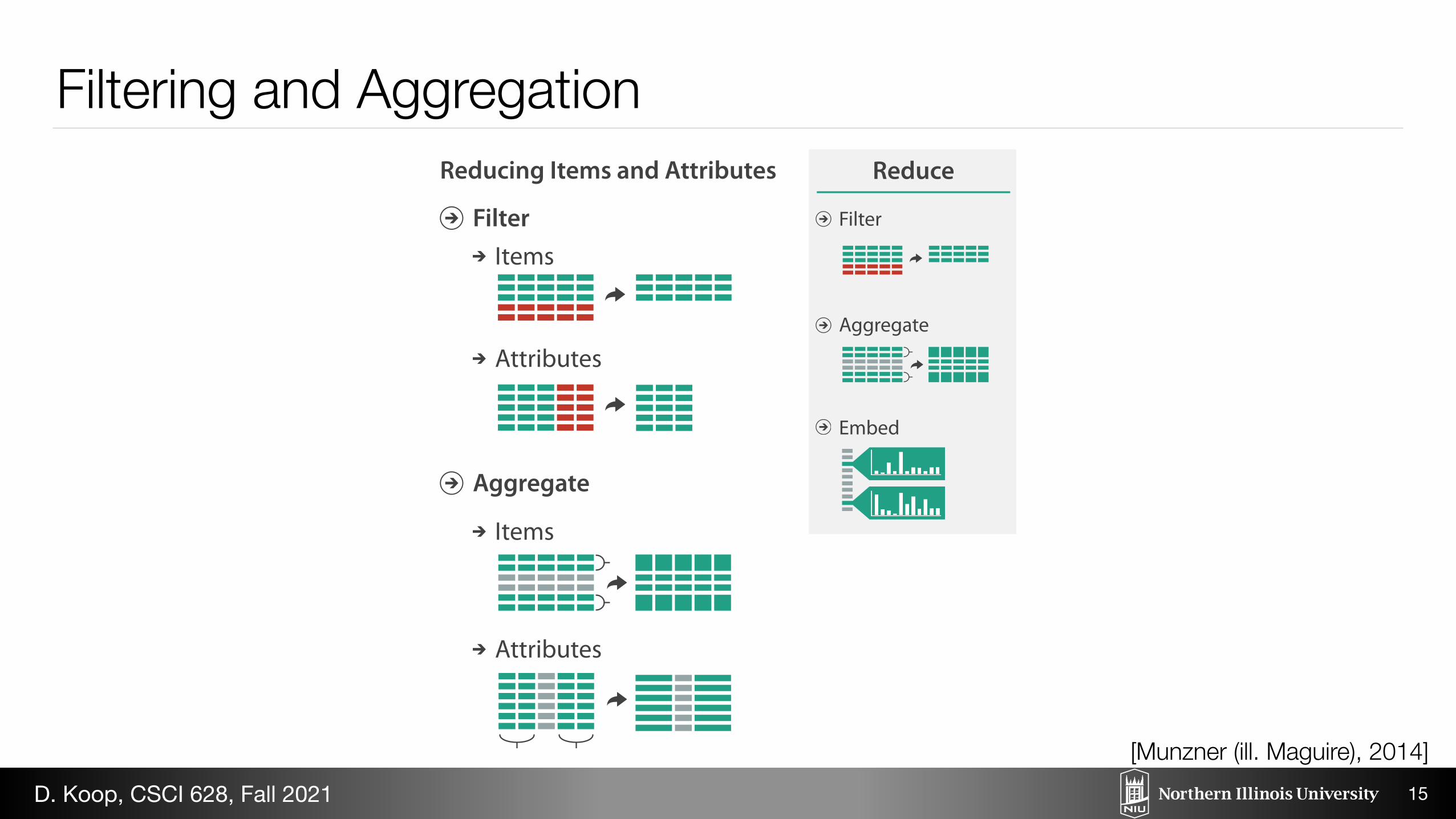
Reduce

Filter

Aggregate

Embed

Reducing Items and Attributes

FilterItems

Attributes

Aggregate

Items

Attributes

Filtering and Aggregation

15


Search All NYTimes.com

FACEBOOK TWITTER GOOGLE+ EMAIL SHARE

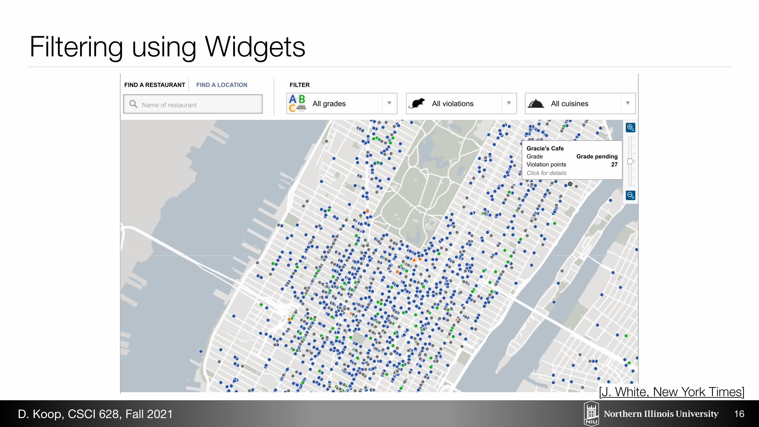
Restaurant locations are derived from the New York City Department of Health and Mental Hygiene database. Due to the limitations of the Health Department’s database, some restaurants couldnot be placed.

By JEREMY WHITE

Source: New York City Department of Health and Mental Hygiene

© 2013 The New York Times Company Site Map Privacy Your Ad Choices Advertise Terms of Sale Terms of Service Work With Us RSS Help Contact Us Site Feedback

New York Health Department Restaurant Ratings MapThe New York City Department of Health and Mental Hygiene performs unannounced sanitary inspections of every restaurant at least once per year.Violation points result in a letter grade, which can be explored in the map below, along with violation descriptions. The information on this map will beupdated every two weeks. For menus and reviews by New York Times critics, visit our restaurants guide. Related Article »

HOME PAGE TODAY'S PAPER VIDEO MOST POPULAR

Dining & WineWORLD U.S. N.Y. / REGION BUSINESS TECHNOLOGY SCIENCE HEALTH SPORTS OPINION ARTS STYLE TRAVEL JOBS REAL ESTATE AUTOS

FASHION & STYLE DINING & WINE HOME & GARDEN WEDDINGS/CELEBRATIONS T MAGAZINESafari Power SaverClick to Start Flash Plug-in

Gracie's CafeGrade Grade pendingViolation points 27Click for details

Gracie's CafeGrade Grade pendingViolation points 27Click for details

Chicken Indian Pizza Improper chemicals14+ points

Name of restaurant All grades All violations All cuisines

FIND A RESTAURANT FIND A LOCATION FILTER

Log In Register Now HelpU.S. Edition

Filtering using Widgets

16

[J. White, New York Times]D. Koop, CSCI 628, Fall 2021

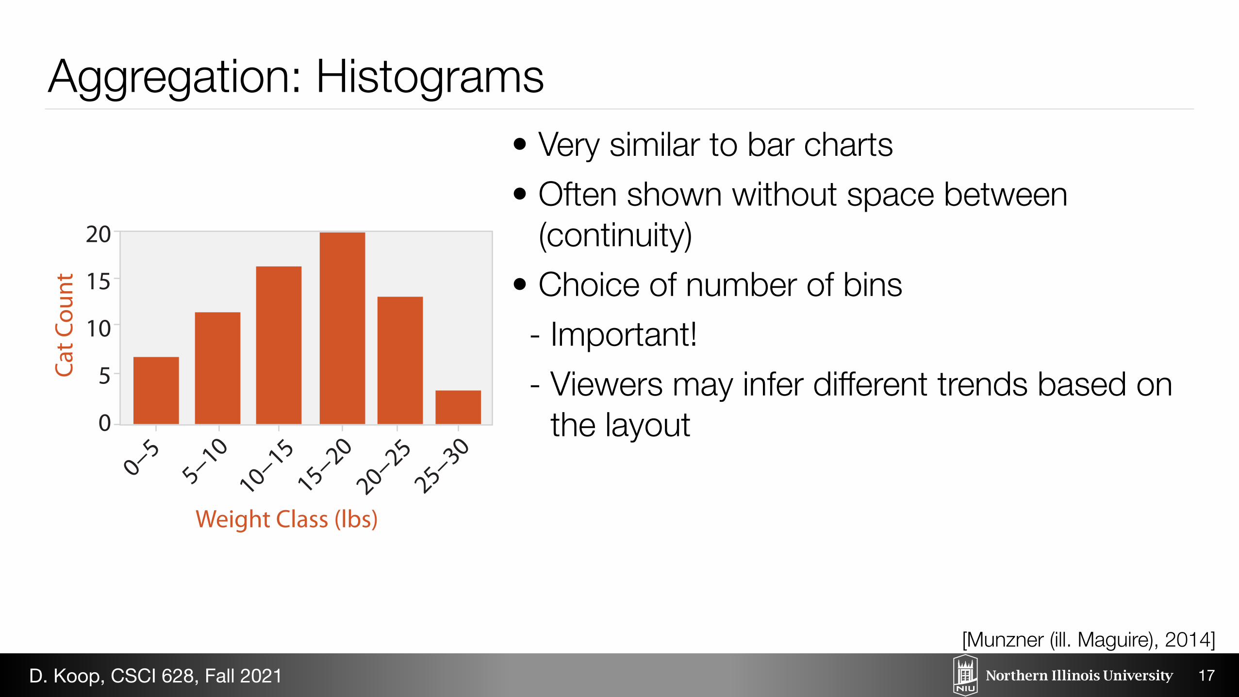
http://archive.nytimes.com/www.nytimes.com/interactive/dining/new-york-health-department-restaurant-ratings-map.html

20

15

10

5

0

Weight Class (lbs)

Aggregation: Histograms• Very similar to bar charts • Often shown without space between

(continuity) • Choice of number of bins - Important! - Viewers may infer different trends based on

the layout

17


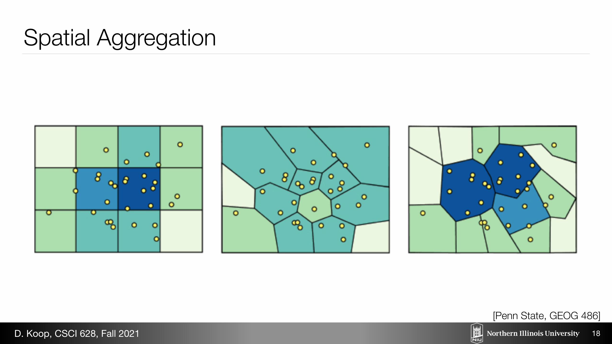
Spatial Aggregation

18

[Penn State, GEOG 486]D. Koop, CSCI 628, Fall 2021

30

spatial aggregation

modifiable areal unit problem in cartography, changing the boundaries of the regions used to analyze data can yield dramatically different results

30

spatial aggregation


30

spatial aggregation


! 2

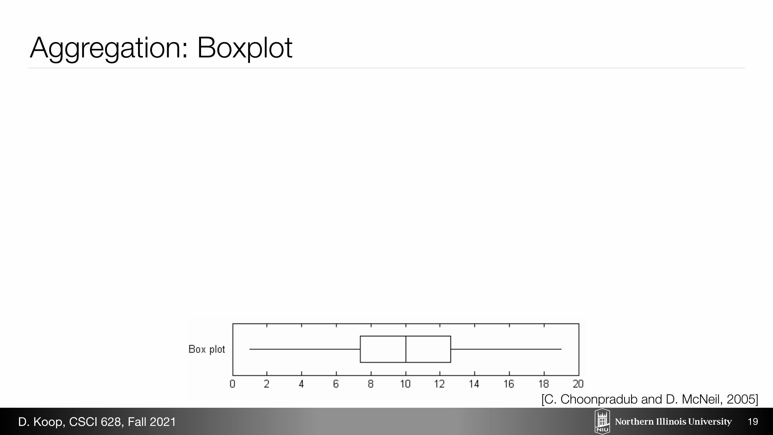
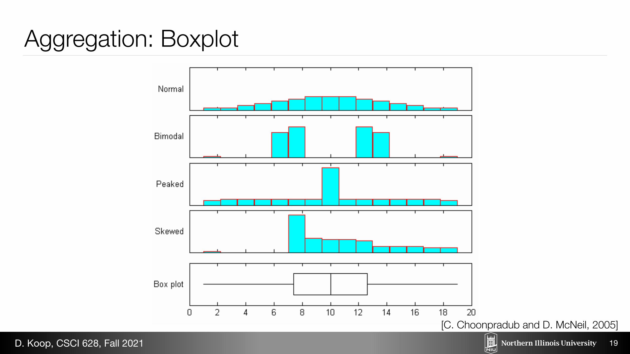
The first sample comprises the normal scores for a sample of this size, scaled to range from 1.0 to 19.0. Sample 2 is a mixture of two identical symmetric clusters of data each of size 49 and centered at 7.4 and 12.6, respectively, together with isolated values at the ends of the range. Sample 3 is a mixture of 70 values spaced evenly over the range, 15 values at 9.5, and 15 values at 10.5. Sample 4 comprises a value at 1.0, 24 values at 7.4, 50 approximately evenly spaced values ranging from 7.4 to 12.6, and 25 approximately evenly spaced values ranging from 12.6 to 19.0.

Figure 1: Histograms and box plot: four samples each of size 100

In an attempt to improve the box plot to show shape information, Benjamini (1988) suggested a “histplot”, obtained by varying the width of the box according to the density of the data at the median and quartiles, where these densities are estimated from a histogram with a small number of bins. Benjamini (1988) also suggested a variation called a “vase plot”, in which the linear segments in the histplot are replaced by smooth curves based on a kernel density estimate. Hintze and Nelson (1998) suggested a further modification called a “violin plot”, which is essentially the same as the vase plot, except that it extends to cover the whole range of the data.

While these methods provide informative and useful displays, in essence they just replace the box plot by a kind of histogram, rather than modifying it. The problem remains to choose the extent of smoothing, which in turn should depend on the sample size.!The box plot has become popular largely because of its simplicity. This raises the question: Is there a simple modification of the box plot that provides better information about the shape of the distribution, especially bimodality?

!

Aggregation: Boxplot

19

[C. Choonpradub and D. McNeil, 2005]D. Koop, CSCI 628, Fall 2021

! 2

The first sample comprises the normal scores for a sample of this size, scaled to range from 1.0 to 19.0. Sample 2 is a mixture of two identical symmetric clusters of data each of size 49 and centered at 7.4 and 12.6, respectively, together with isolated values at the ends of the range. Sample 3 is a mixture of 70 values spaced evenly over the range, 15 values at 9.5, and 15 values at 10.5. Sample 4 comprises a value at 1.0, 24 values at 7.4, 50 approximately evenly spaced values ranging from 7.4 to 12.6, and 25 approximately evenly spaced values ranging from 12.6 to 19.0.

Figure 1: Histograms and box plot: four samples each of size 100

In an attempt to improve the box plot to show shape information, Benjamini (1988) suggested a “histplot”, obtained by varying the width of the box according to the density of the data at the median and quartiles, where these densities are estimated from a histogram with a small number of bins. Benjamini (1988) also suggested a variation called a “vase plot”, in which the linear segments in the histplot are replaced by smooth curves based on a kernel density estimate. Hintze and Nelson (1998) suggested a further modification called a “violin plot”, which is essentially the same as the vase plot, except that it extends to cover the whole range of the data.

While these methods provide informative and useful displays, in essence they just replace the box plot by a kind of histogram, rather than modifying it. The problem remains to choose the extent of smoothing, which in turn should depend on the sample size.!The box plot has become popular largely because of its simplicity. This raises the question: Is there a simple modification of the box plot that provides better information about the shape of the distribution, especially bimodality?

!

Aggregation: Boxplot

19

[C. Choonpradub and D. McNeil, 2005]D. Koop, CSCI 628, Fall 2021

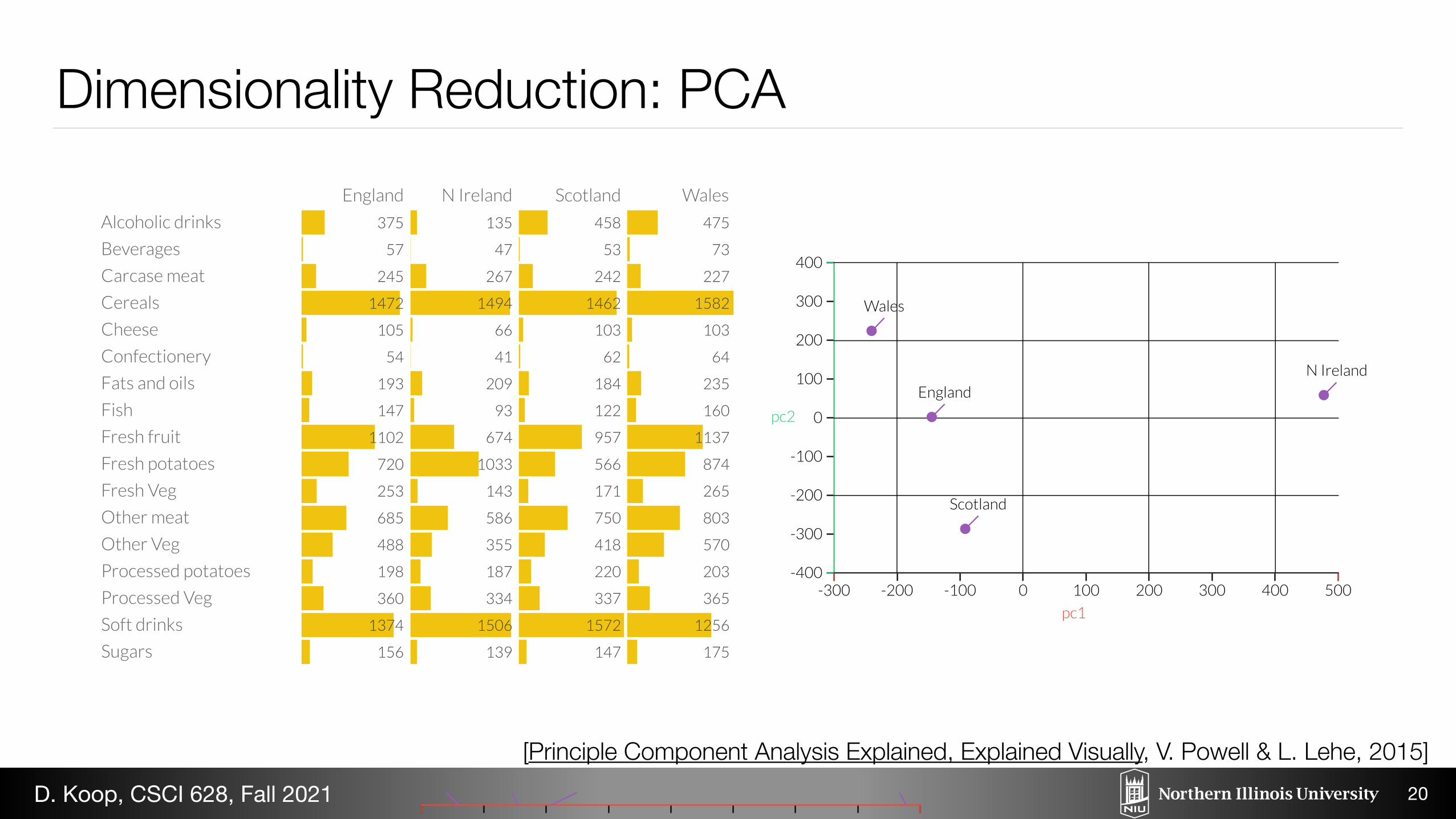
Dimensionality Reduction: PCA

20

[Principle Component Analysis Explained, Explained Visually, V. Powell & L. Lehe, 2015]D. Koop, CSCI 628, Fall 2021

375

57

245

1472

105

54

193

147

1102

720

253

685

488

198

360

1374

156

135

47

267

1494

66

41

209

93

674

1033

143

586

355

187

334

1506

139

458

53

242

1462

103

62

184

122

957

566

171

750

418

220

337

1572

147

475

73

227

1582

103

64

235

160

1137

874

265

803

570

203

365

1256

175

England N Ireland Scotland Wales

Alcoholic drinks

Beverages

Carcase meat

Cereals

Cheese

Confectionery

Fats and oils

Fish

Fresh fruit

Fresh potatoes

Fresh Veg

Other meat

Other Veg

Processed potatoes

Processed Veg

Soft drinks

Sugars

Email address

Here's the plot of the data along the first principal component. Already we can see something is different about Northern Ireland.

-300 -200 -100 0 100 200 300 400 500pc1

EnglandWales Scotland N Ireland

Now, see the first and second principal components, we see Northern Ireland a major outlier. Once we go back and look at the datain the table, this makes sense: the Northern Irish eat way more grams of fresh potatoes and way fewer of fresh fruits, cheese, fishand alcoholic drinks. It's a good sign that structure we've visualized reflects a big fact of real-world geography: Northern Ireland isthe only of the four countries not on the island of Great Britain. (If you're confused about the differences among England, the UKand Great Britain, see: this video.)

-300 -200 -100 0 100 200 300 400 500-400

-300

-200

-100

0

100

200

300

400

pc1

pc2

England

Wales

Scotland

N Ireland

For more explanations, visit the Explained Visually project homepage.

Or subscribe to our mailing list.

Subscribe

375

57

245

1472

105

54

193

147

1102

720

253

685

488

198

360

1374

156

135

47

267

1494

66

41

209

93

674

1033

143

586

355

187

334

1506

139

458

53

242

1462

103

62

184

122

957

566

171

750

418

220

337

1572

147

475

73

227

1582

103

64

235

160

1137

874

265

803

570

203

365

1256

175

England N Ireland Scotland Wales

Alcoholic drinks

Beverages

Carcase meat

Cereals

Cheese

Confectionery

Fats and oils

Fish

Fresh fruit

Fresh potatoes

Fresh Veg

Other meat

Other Veg

Processed potatoes

Processed Veg

Soft drinks

Sugars

Email address

Here's the plot of the data along the first principal component. Already we can see something is different about Northern Ireland.

-300 -200 -100 0 100 200 300 400 500pc1

EnglandWales Scotland N Ireland

Now, see the first and second principal components, we see Northern Ireland a major outlier. Once we go back and look at the datain the table, this makes sense: the Northern Irish eat way more grams of fresh potatoes and way fewer of fresh fruits, cheese, fishand alcoholic drinks. It's a good sign that structure we've visualized reflects a big fact of real-world geography: Northern Ireland isthe only of the four countries not on the island of Great Britain. (If you're confused about the differences among England, the UKand Great Britain, see: this video.)

-300 -200 -100 0 100 200 300 400 500-400

-300

-200

-100

0

100

200

300

400

pc1

pc2

England

Wales

Scotland

N Ireland

For more explanations, visit the Explained Visually project homepage.

Or subscribe to our mailing list.

Subscribe

http://setosa.io/ev/principal-component-analysis/

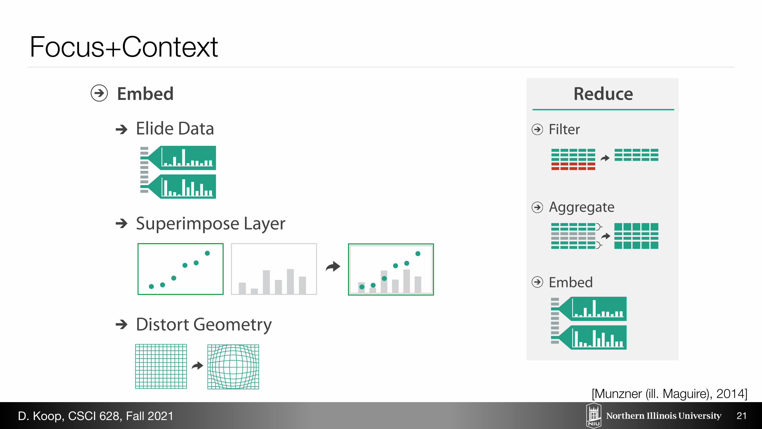
Embed

Elide Data

Superimpose Layer

Distort Geometry

Reduce

Filter

Aggregate

Embed

Focus+Context

21


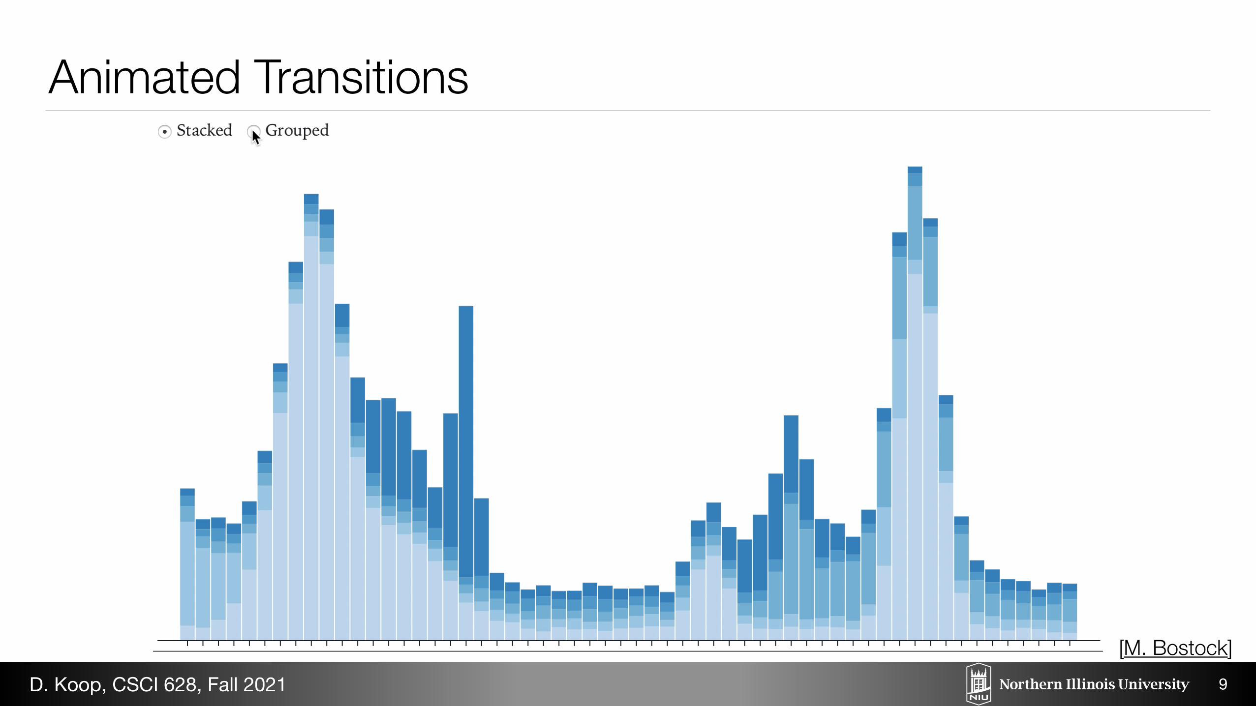
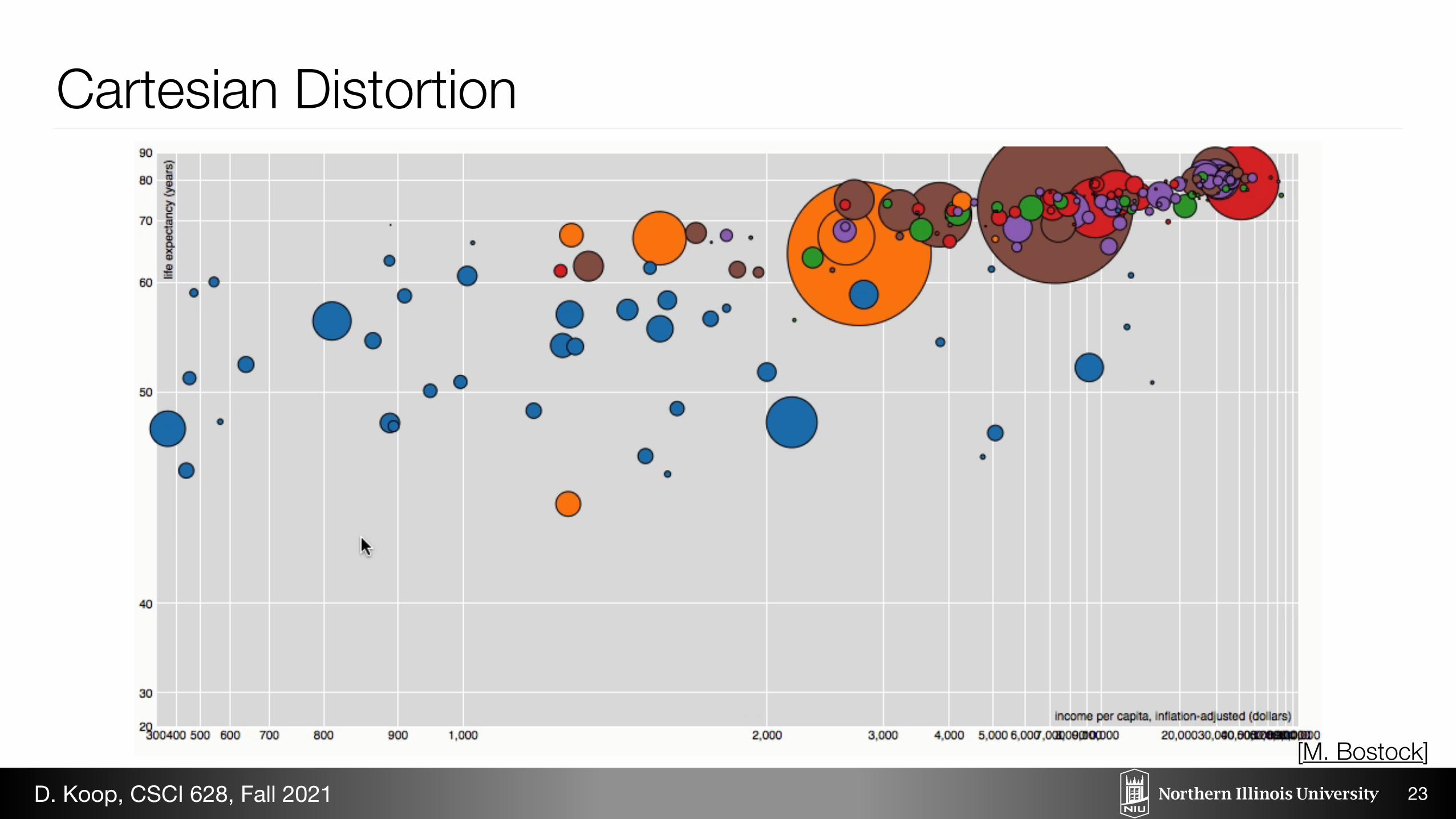
June 21, 2012 / Mike Bostock

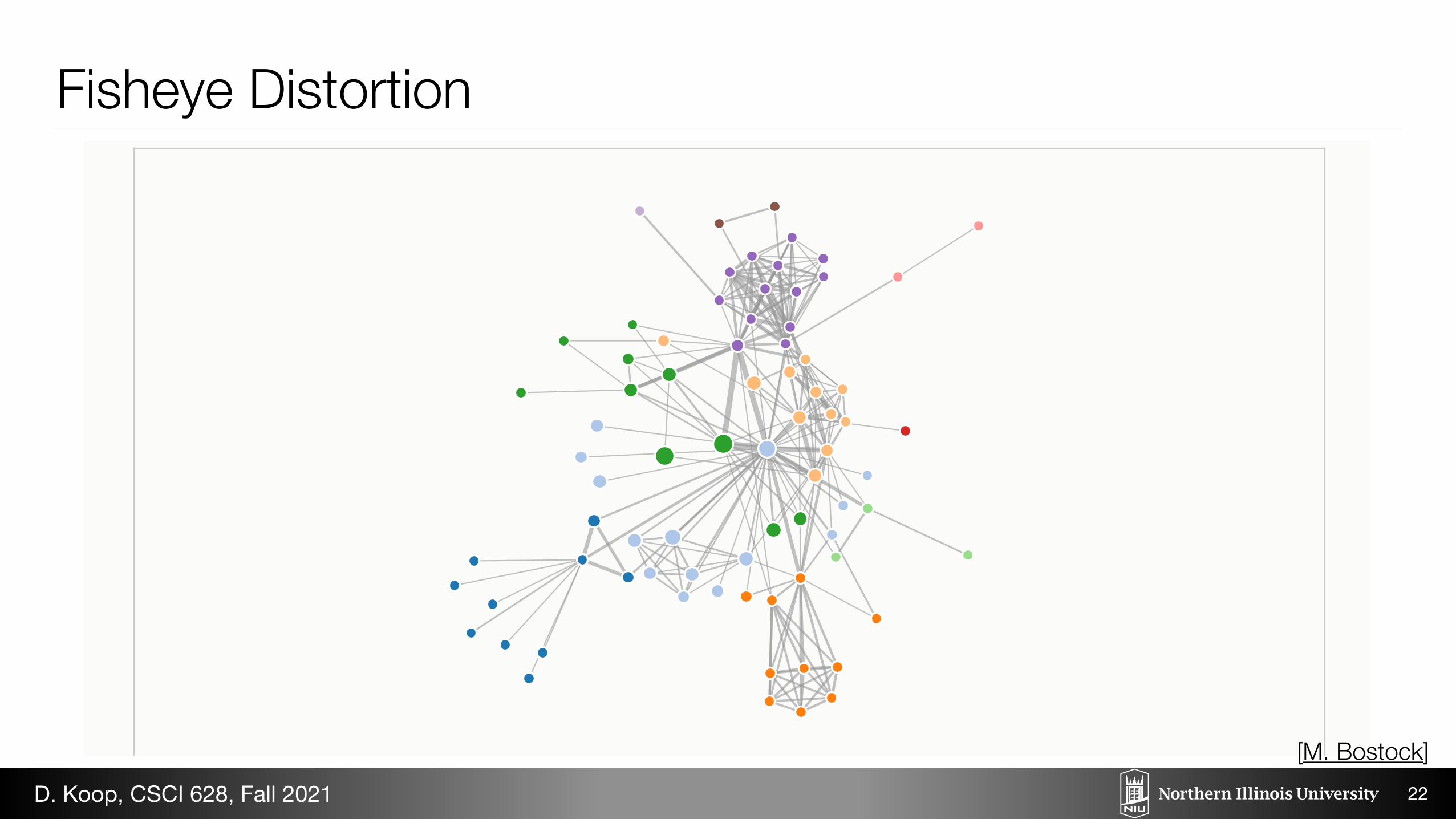
Fisheye Distortion

It can be difficult to observe micro and macro features simultaneously with complex graphs. If youzoom in for detail, the graph is too big to view in its entirety. If you zoom out to see the overallstructure, small details are lost. Focus + context techniques allow interactive exploration of an area

Mouseover to distort the nodes.

Fisheye Distortion

22


http://bost.ocks.org/mike/fisheye/

Cartesian Distortion

23



Cartesian Distortion

23



24

The purpose of visualization is about insight, not pictures

– B. Shneiderman


25

Visualization Research


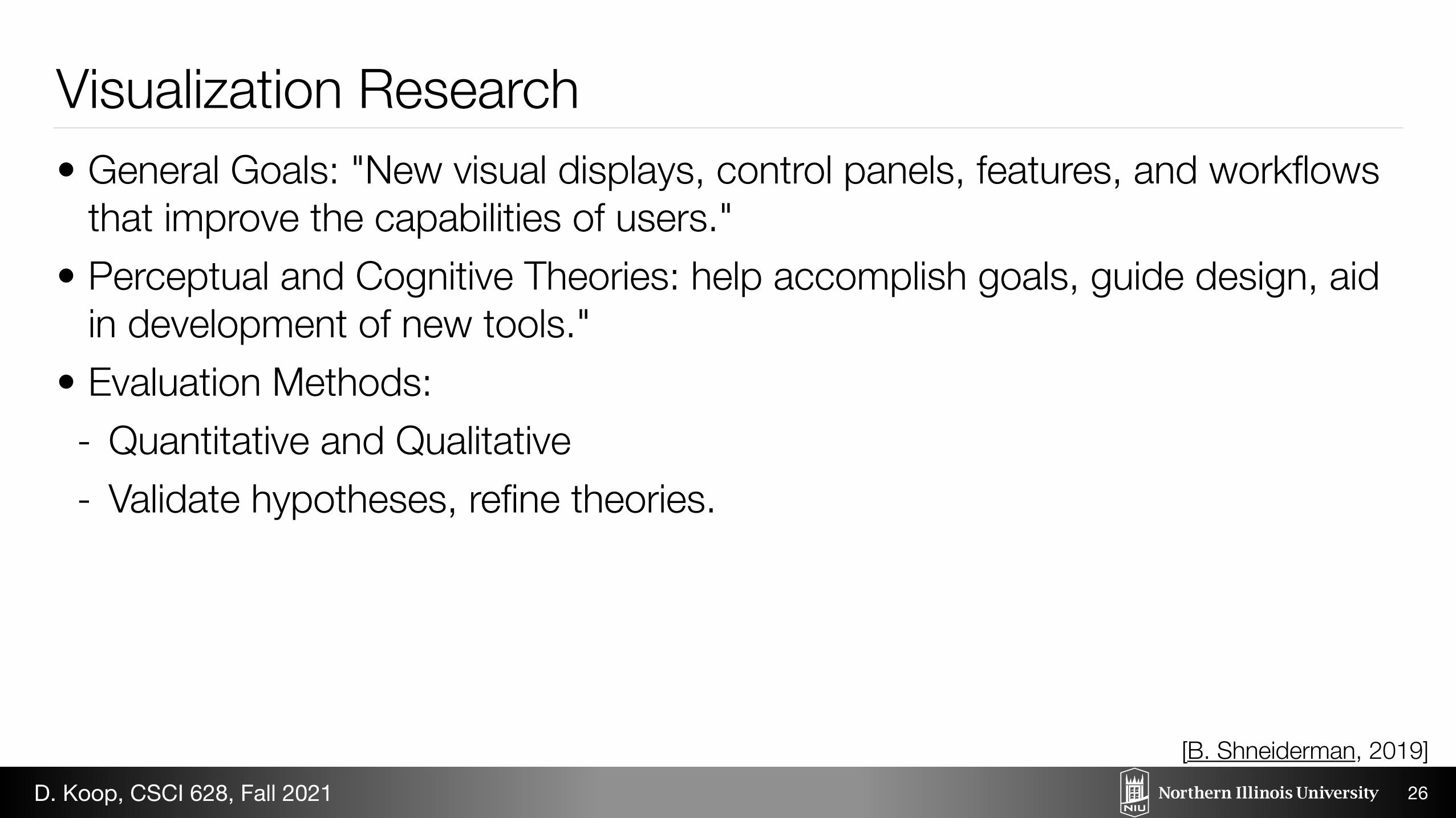
Visualization Research• General Goals: "New visual displays, control panels, features, and workflows

that improve the capabilities of users." • Perceptual and Cognitive Theories: help accomplish goals, guide design, aid

in development of new tools." • Evaluation Methods: - Quantitative and Qualitative - Validate hypotheses, refine theories.

26

[B. Shneiderman, 2019]D. Koop, CSCI 628, Fall 2021

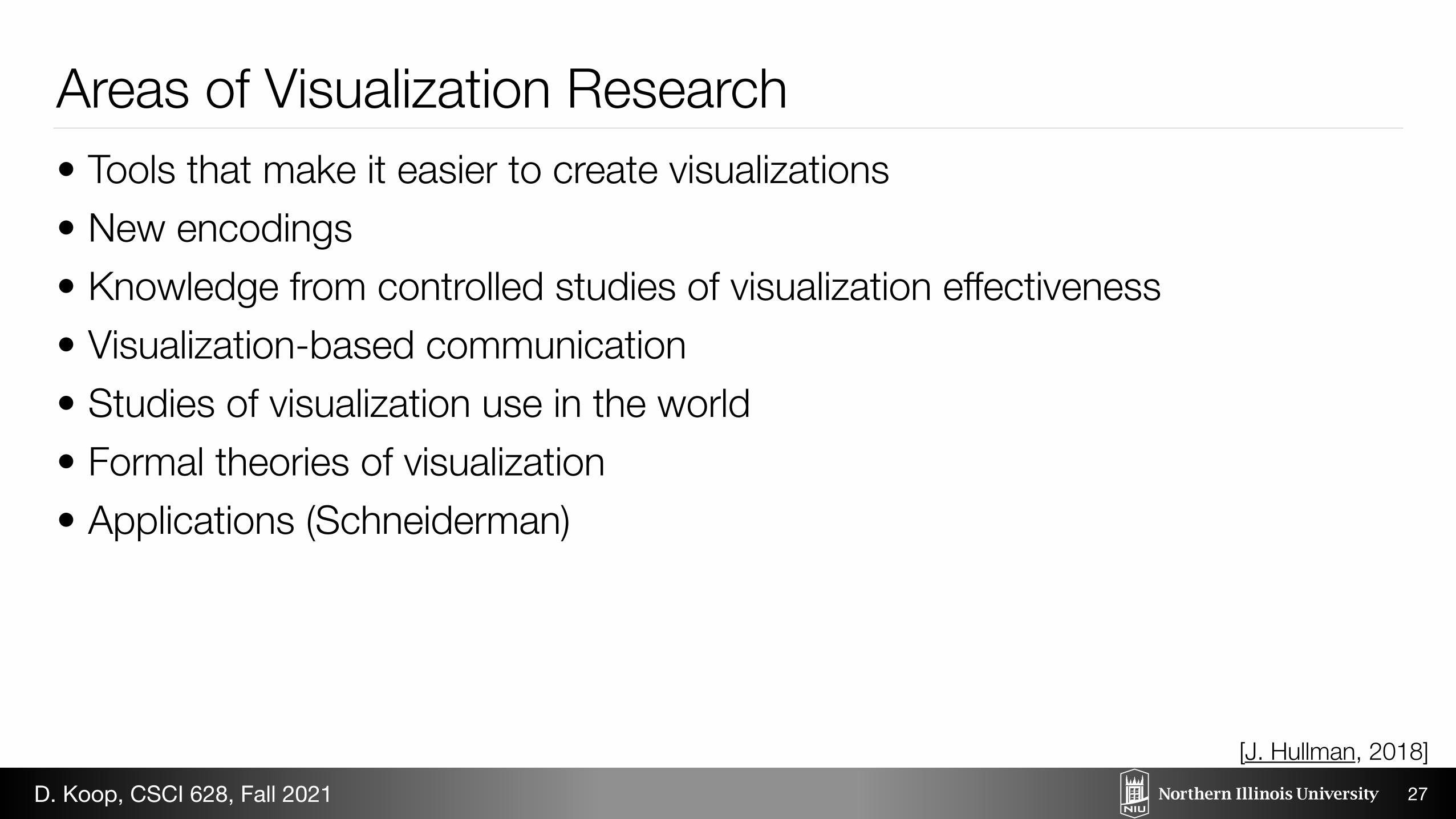
https://interactions.acm.org/blog/view/the-purpose-of-visualization-is-insight-not-pictures-an-interview-with-ben

Areas of Visualization Research• Tools that make it easier to create visualizations • New encodings • Knowledge from controlled studies of visualization effectiveness • Visualization-based communication • Studies of visualization use in the world • Formal theories of visualization • Applications (Schneiderman)

27

[J. Hullman, 2018]D. Koop, CSCI 628, Fall 2021

https://medium.com/multiple-views-visualization-research-explained/what-is-visualization-research-what-should-it-be-8840a9ba658

Tools that make it easier to create visualizations• Tableau, Spotfire, D3 were all proposed and developed by visualization

researchers • Not just create visualizations, but effective visualizations • Current Trends: - Web-based frameworks - Declarative, more concise specification (Vega-Lite)

28



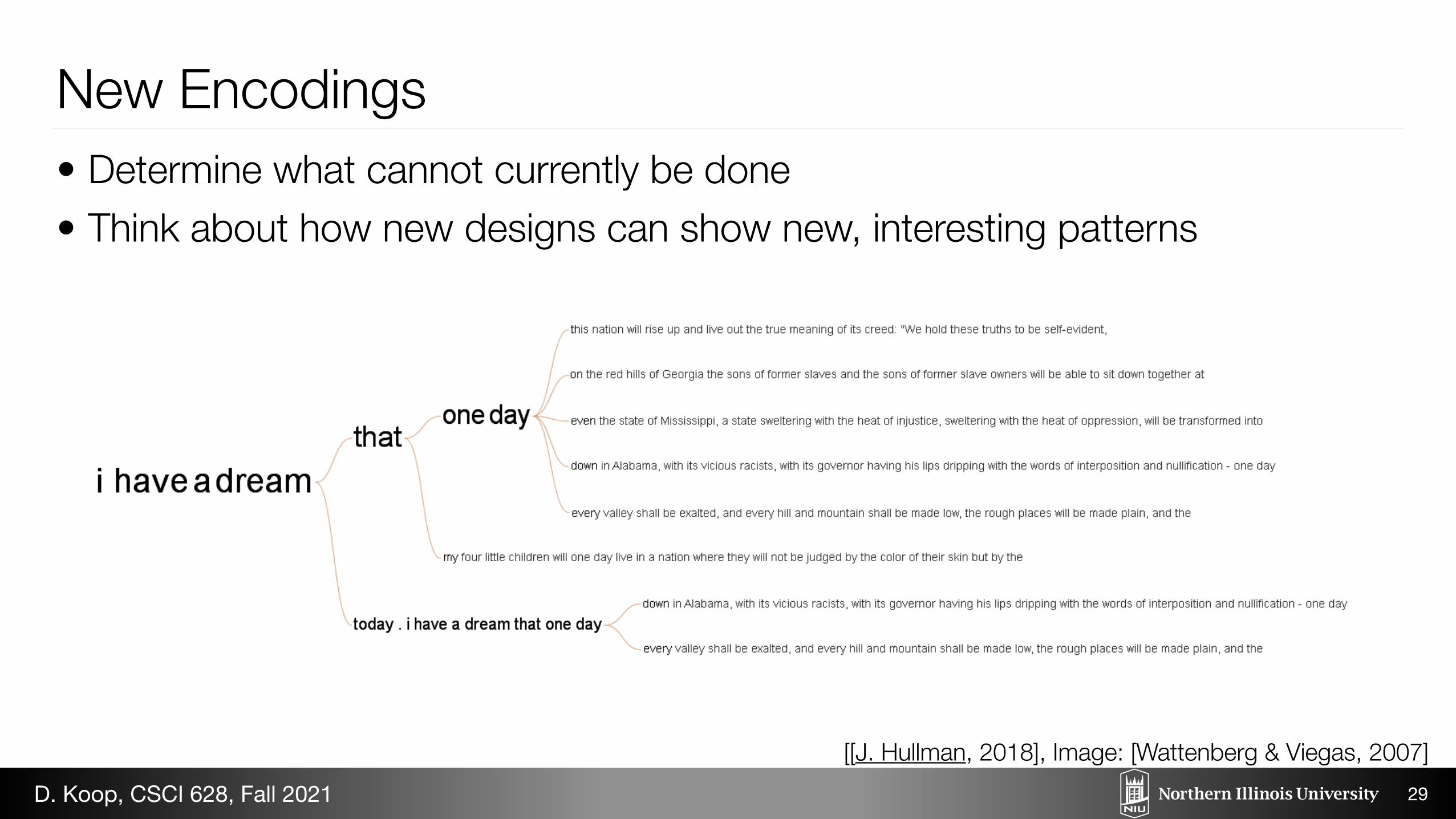
New Encodings• Determine what cannot currently be done • Think about how new designs can show new, interesting patterns

29

[[J. Hullman, 2018], Image: [Wattenberg & Viegas, 2007] D. Koop, CSCI 628, Fall 2021

on Many Eyes, for instance, we would not have guessed at the popularity of religious analyses. Given the broad demand for text visualizations, however, it seems like a fruitful area of study.

ACKNOWLEDGEMENTS The authors thank Frank van Ham, Jesse Kriss, Matt McKeon, Lee Byron, and Eric Gilbert for helpful suggestions. In addition, we are grateful to the users of Many Eyes for their creativity and willingness to provide feedback on an experimental visualization technique.

Fig 10: Word Tree showing all occurrences of “I have a dream” in Martin Luther King’s historical speech.

Fig 9. Word tree of the King James Bible showing all occurrences of “love the.”


Knowledge from studies of visualization effectiveness

30

534 Journal of the American Statistical Association, September 1984

TYPE 1 TYPE 2 TYPE 3 TYPE 4 TYPE 5

100o 10oo 100- 10oo 100-

IhLL O_ 0A A * A B A B A B A B A B

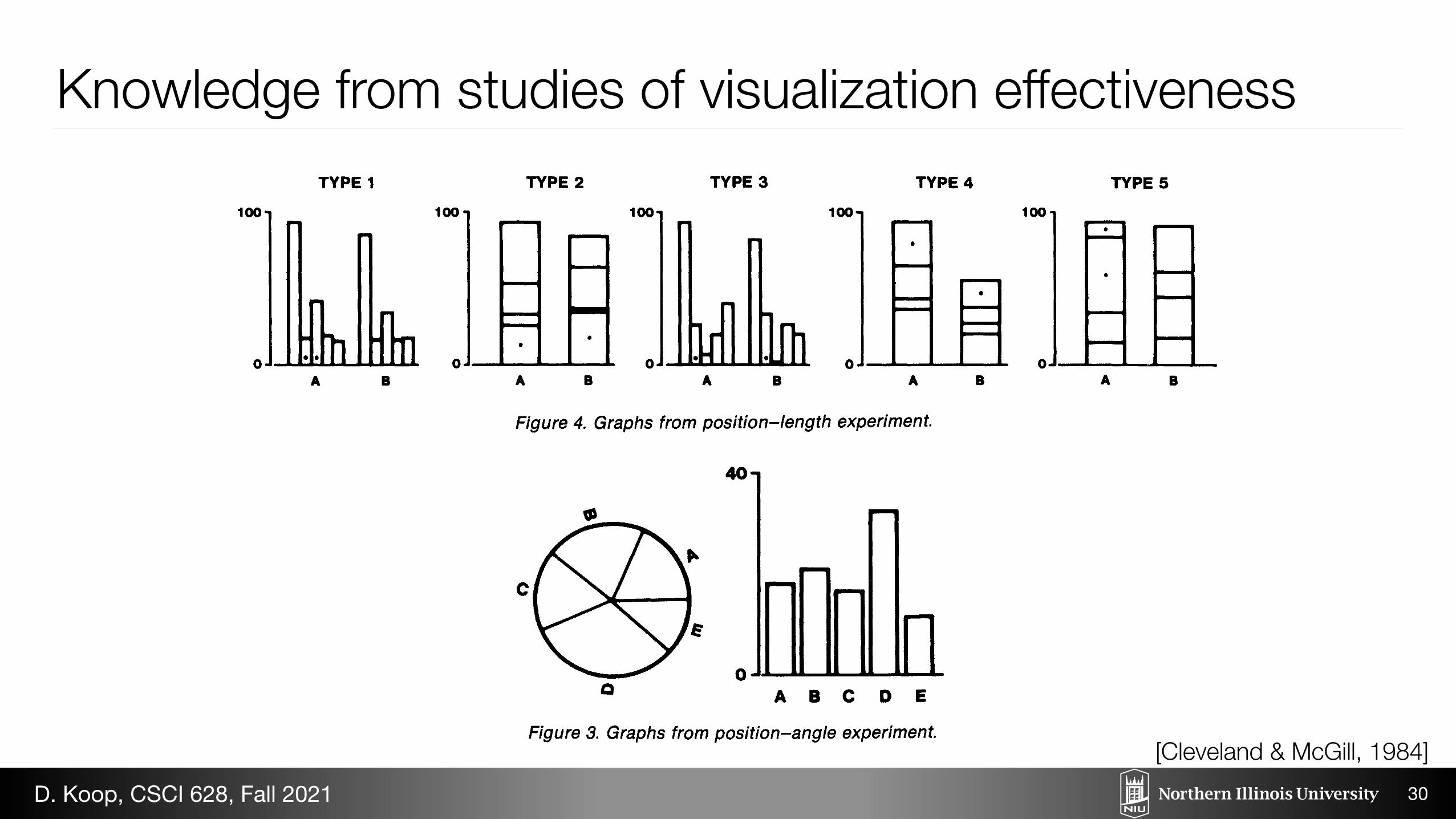
Figure 4. Graphs from position-length experiment.

tracted by perceiving position along a scale, in this case the horizontal axis. The y values can be perceived in a similar manner.

The real power of a Cartesian graph, however, does not derive only from one's ability to perceive the x and y values separately but, rather, from one's ability to un- derstand the relationship of x and y. For example, in Fig- ure 7 we see that the relationship is nonlinear and see the nature of that nonlinearity. The elementary task that enables us to do this is perception of direction. Each pair of points on the plot, (xi, yi) and (xj, yj), with xi =$ Xj, has an associated slope

(yj - y)(xj - xi).

The eye-brain system is capable of extracting such a slope by perceiving the direction of the line segment join- ing (xi, yi) and (xj, yj). We conjecture that the perception of these slopes allows the eye-brain system to imagine a smooth curve through the points, which is then used to judge the pattern. For example, in Figure 7 one can perceive that the slopes for pairs of points on the left side of the plot are greater than those on the right side of the plot, which is what enables one to judge that the relationship is nonlinear.

That the elementary task of judging directions on a Cartesian graph is vital for understanding the relationship of x and y is demonstrated in Figure 8. The same x and y values are shown by paired bars. As with the Cartesian

MURDER RATES, 1978

8.5 FIVE REPRESETIV SHADINGS- _ , _,

RE 12.1_

-~ 1 5.8- RATES PER 100,000 POPULATION

Figure 5. Statistical map with shading.

This content downloaded from 134.88.249.216 on Thu, 12 Feb 2015 23:18:30 PMAll use subject to JSTOR Terms and Conditions

Cleveland and McGill: Graphical Perception 533

0

-i S

to

I

5 10 15

MUROER RATE

Figure 2. Sample distribution function of 1978 murder rate.

judging position along a common scale, which in this case is the horizontal scale.

Bar Charts

Figures 3 and 4 contain bar charts that were shown to subjects in perceptual experiments. The few noticeable peculiarities are there for purposes of the experiments, described in a later section.

Judging position is a task used to extract the values of the data in the bar chart in the right panel of Figure 3. But now the graphical elements used to portray the data-the bars-also change in length and area. We conjecture that the primary elementary task is judging position along a common scale, but judgments of area and length probably also play a role.

Pie Charts

The left panel of Figure 3 is a pie chart, one of the most commonly used graphs for showing the relative sizes of the parts of a whole. For this graph we conjecture that the primary elementary visual task for extracting the nu- merical information is perception of angle, but the areas and arc lengths of the pie slices are variable and probably are also involved in judging the data.

Divided Bar Charts

Figure 4 has three div'ided bar charts (Types 2, 4, and 5). For each of the three, the totals of A and B can be compared by perceiving position along the scale. Position judgments can also be used to compare the two bottom

diviionsin ech cse; or Tpe 2the otto divsin are arkd wth ots.Allothr vluesmus becomare by he lemntay tsk f prcevin difernt ar enghs

examples are the two divisions marked with dots in Type 4 and the two marked in Type 5.

Statistical Maps With Shading

A chart frequently used to portray information as a function of geographical location is a statistical map with shading, such as Figure 5 (from Gale and Halperin 1982), which shows the murder data of Figure 2. Values of a real variable are encoded by filling in geographical regions using any one of many techniques that produce gray-scale shadings. In Figure 5 the technique illustrated uses grids drawn with different spacings; the data are not proportional to the grid spacing but, rather, to a compli- cated function of spacing. We conjecture that the primary elementary task used to extract the data in this case is the perception of shading, but judging the sizes of the squares formed by the grids probably also plays a role, particularly for the large squares.

Curve-Difference Charts

Another class of commonly used graphs is curve-difference charts: Two or more curves are drawn on the graph, and vertical differences between some of the curves encode real variables that are to be extracted. One type of curve-difference chart is a divided, or aggregate, line chart (Monkhouse and Wilkinson 1963), which is typ- ically used to show how parts of a whole change through time.

Figure 6 is a curve-difference chart. The original was drawn by William Playfair; because our photograph of the original was of poor quality, we had the figure re- drafted, trying to keep as close to the original as possible. The two curves portray exports from England to the East Indies and imports to England from the East Indies. The vertical distances between the two curves, which encode the export-import imbalance, are highlighted. The quantitative information about imports and exports is extracted by perceiving position along a common scale, and the information about the imbalances is extracted by perceiving length, that is, vertical distance between the two curves.

Cartesian Graphs and Why They Work

Figure 7 is a Cartesian graph of paired values of two variables, x and y. The values of x can be visually ex-

40

c< 0WBHEl a A BC D E

Figure 3. Graphs from position-angle experiment.

This content downloaded from 134.88.249.216 on Thu, 12 Feb 2015 23:18:30 PMAll use subject to JSTOR Terms and Conditions

[Cleveland & McGill, 1984]D. Koop, CSCI 628, Fall 2021

Evaluating the Impact of Binning 2D Scalar FieldsLace Padilla, P. Samuel Quinan, Miriah Meyer, and Sarah H. Creem-Regehr

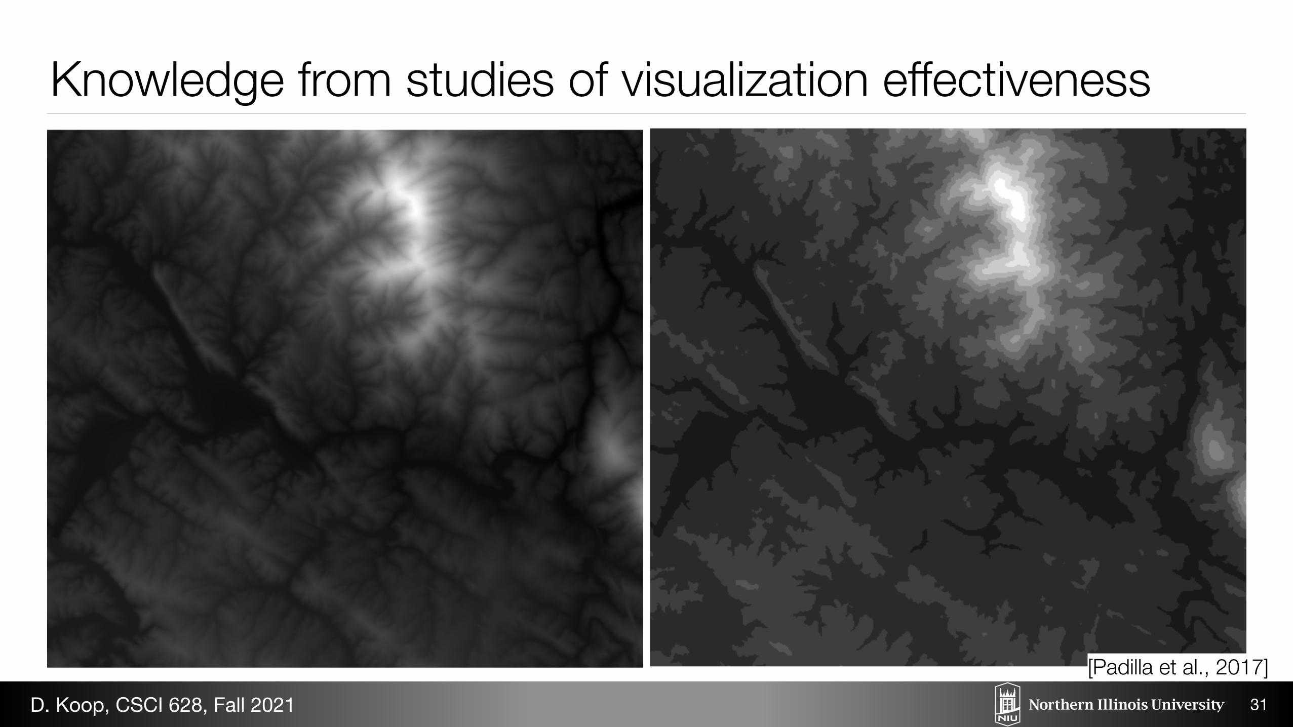
Fig. 1: Experimental stimuli for five binning conditions: A. Continuous, B. 10m binning, C. 20m binning, D. 30m binning, E. 40mbinning

Abstract— The expressiveness principle for visualization design asserts that a visualization should encode all of the available data,and only the available data, implying that continuous data types should be visualized with a continuous encoding channel. And yet,in many domains binning continuous data is not only pervasive, but it is accepted as standard practice. Prior work provides no clearguidance for when encoding continuous data continuously is preferable to employing binning techniques or how this choice affectsdata interpretation and decision making. In this paper, we present a study aimed at better understanding the conditions in whichthe expressiveness principle can or should be violated for visualizing continuous data. We provided participants with visualizationsemploying either continuous or binned greyscale encodings of geospatial elevation data and compared participants’ ability to completea wide variety of tasks. For various tasks, the results indicate significant differences in decision making, confidence in responses, andtask completion time between continuous and binned encodings of the data. In general, participants with continuous encodings werefaster to complete many of the tasks, but never outperformed those with binned encodings, while performance accuracy with binnedencodings was superior to continuous encodings in some tasks. These findings suggest that strict adherence to the expressivenessprinciple is not always advisable. We discuss both the implications and limitations of our results and outline various avenues forpotential work needed to further improve guidelines for using continuous versus binned encodings for continuous data types.

Index Terms—Geographic/Geospatial Visualization, Qualitative Evaluation, Color Perception, Perceptual Cognition

1 INTRODUCTION

A foundational design principle in visualization is the expressivenessprinciple, which states that a visual encoding should express all of therelationships in the data, and only the relationships in the data [24, 35].For a continuous data type, this implies that a continuous encodingchannel is a good choice. In practice, however, domains such as car-

• L. Padilla is with the University of Utah Department of Psychology.E-mail: [email protected]

• S. Quinan and M. Meyer are with the University of Utah School ofComputing. E-mail: psq,[email protected].

• S. Creem-Regehr is with the University of Utah Department of Psychology.E-mail: [email protected].

Manuscript received xx xxx. 201x; accepted xx xxx. 201x. Date ofPublication xx xxx. 201x; date of current version xx xxx. 201x.For information on obtaining reprints of this article, please sende-mail to: [email protected] Object Identifier: xx.xxxx/TVCG.201x.xxxxxxx/

tography [43] and meteorology [36] have strong conventions that visu-alize continuous data with a discrete encoding. These domains rely onvisual channels, such as color and saturation to encode a continuousfunction defined over two-dimensional space, known as a 2D scalarfield. They commonly do so by employing discrete colormaps or con-tour lines, also called isarithmic maps [43].

Existing literature provides little guidance about encoding contin-uous, 2D scalar fields with binned colormaps, or how this design de-cision affects data interpretation and decision making. Research intoproperties of colormaps for encoding continuous data types has largelyfocused on continuous colormaps [2, 28, 38, 48]. This line of researchprovides guidance on how to capture properties of the data, such asdivergence around a center point [48] or emphasis on one end of thedata range [2]. These papers go so far as proposing correspondingbinned colormaps, but do not make claims, or even discuss, their ef-ficacy for continuous data. Work on transfer function design has alsoproposed methods for binning colors, but with a focus on volumetricscalar fields, with the underlying goal of classifying materials or fea-tures [12], as opposed to directly understanding the continuous nature

Knowledge from studies of visualization effectiveness

31

Evaluating the Impact of Binning 2D Scalar FieldsLace Padilla, P. Samuel Quinan, Miriah Meyer, and Sarah H. Creem-Regehr

Fig. 1: Experimental stimuli for five binning conditions: A. Continuous, B. 10m binning, C. 20m binning, D. 30m binning, E. 40mbinning

Abstract— The expressiveness principle for visualization design asserts that a visualization should encode all of the available data,and only the available data, implying that continuous data types should be visualized with a continuous encoding channel. And yet,in many domains binning continuous data is not only pervasive, but it is accepted as standard practice. Prior work provides no clearguidance for when encoding continuous data continuously is preferable to employing binning techniques or how this choice affectsdata interpretation and decision making. In this paper, we present a study aimed at better understanding the conditions in whichthe expressiveness principle can or should be violated for visualizing continuous data. We provided participants with visualizationsemploying either continuous or binned greyscale encodings of geospatial elevation data and compared participants’ ability to completea wide variety of tasks. For various tasks, the results indicate significant differences in decision making, confidence in responses, andtask completion time between continuous and binned encodings of the data. In general, participants with continuous encodings werefaster to complete many of the tasks, but never outperformed those with binned encodings, while performance accuracy with binnedencodings was superior to continuous encodings in some tasks. These findings suggest that strict adherence to the expressivenessprinciple is not always advisable. We discuss both the implications and limitations of our results and outline various avenues forpotential work needed to further improve guidelines for using continuous versus binned encodings for continuous data types.

Index Terms—Geographic/Geospatial Visualization, Qualitative Evaluation, Color Perception, Perceptual Cognition

1 INTRODUCTION

A foundational design principle in visualization is the expressivenessprinciple, which states that a visual encoding should express all of therelationships in the data, and only the relationships in the data [24, 35].For a continuous data type, this implies that a continuous encodingchannel is a good choice. In practice, however, domains such as car-

• L. Padilla is with the University of Utah Department of Psychology.E-mail: [email protected]

• S. Quinan and M. Meyer are with the University of Utah School ofComputing. E-mail: psq,[email protected].

• S. Creem-Regehr is with the University of Utah Department of Psychology.E-mail: [email protected].

Manuscript received xx xxx. 201x; accepted xx xxx. 201x. Date ofPublication xx xxx. 201x; date of current version xx xxx. 201x.For information on obtaining reprints of this article, please sende-mail to: [email protected] Object Identifier: xx.xxxx/TVCG.201x.xxxxxxx/

tography [43] and meteorology [36] have strong conventions that visu-alize continuous data with a discrete encoding. These domains rely onvisual channels, such as color and saturation to encode a continuousfunction defined over two-dimensional space, known as a 2D scalarfield. They commonly do so by employing discrete colormaps or con-tour lines, also called isarithmic maps [43].

Existing literature provides little guidance about encoding contin-uous, 2D scalar fields with binned colormaps, or how this design de-cision affects data interpretation and decision making. Research intoproperties of colormaps for encoding continuous data types has largelyfocused on continuous colormaps [2, 28, 38, 48]. This line of researchprovides guidance on how to capture properties of the data, such asdivergence around a center point [48] or emphasis on one end of thedata range [2]. These papers go so far as proposing correspondingbinned colormaps, but do not make claims, or even discuss, their ef-ficacy for continuous data. Work on transfer function design has alsoproposed methods for binning colors, but with a focus on volumetricscalar fields, with the underlying goal of classifying materials or fea-tures [12], as opposed to directly understanding the continuous nature

[Padilla et al., 2017]D. Koop, CSCI 628, Fall 2021

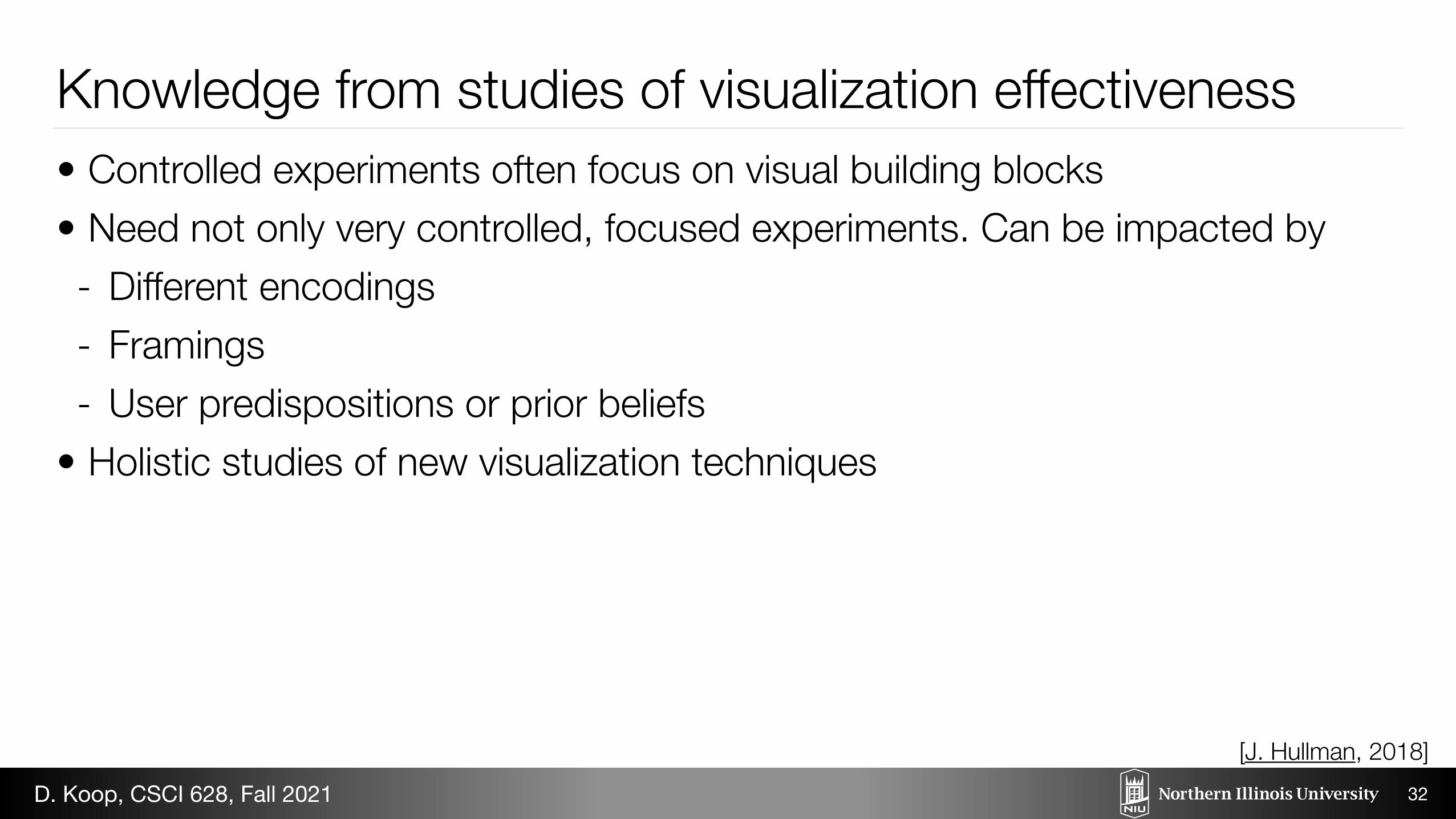
Knowledge from studies of visualization effectiveness• Controlled experiments often focus on visual building blocks • Need not only very controlled, focused experiments. Can be impacted by - Different encodings - Framings - User predispositions or prior beliefs

• Holistic studies of new visualization techniques

32



Supporting Visual Analytics• Exploratory Data Analysis • Sensemaking & Meaning-making • Interpretability of Machine Learning Models

33



3.2 Qualitative Analysis To inform the design of a tool that suggests good story structures with insights on the strategies of professional designers, we conduct-ed a qualitative analysis of the structural aspects of 42 examples of explicitly-guided (i.e., unambiguously linearly ordered) professional narrative visualizations. The study poses several questions about sequencing in professional narrative visualization presentations: • What types of changes (transition types) drive between-

visualization transitions in linear narrative visualizations? • Are there general characteristics that are shared among the

common types of transitions? • How do strategies for local (visualization-to-visualization)

transitions compare to global transitions (patterns involving multiple local transitions)?

3.2.1 Study Design 42 narrative visualizations created between 2006 and 2012 were compiled (full list in supplementary file). We seeded the set with visualizations in an independently-curated sample of New York Times (NYT) and Guardian interactives [23]. Additional examples came from visualization blogs and repositories (e.g., visualizing.org) and well-known news sources (e.g., BBC). We included only visual-izations with non-ambiguous sequencing cues like numbered slides or steps across linked views, a “Next,” “→,” or “Continue” button, or a “Play” button for a self-running video or slideshow. These features had to occur without additional navigational choices. Interactive slideshows formed the largest format in our sample (23/42), with other presentations including animated data videos (7/42) and inter-active timelines (6/42), live narrated visualization presentations (1/42), and static slideshows archived online but originally intended for live presentation (5/42).

While the individual states that comprise a visualization sequence are fairly unambiguous in a slideshow-style presentation, the constit-uent states of smooth animated narrative visualizations are more difficult to identify. A visualization state has been defined as a set of parameters applied to data [14], or the settings of interface widgets in a visualization environment along with the application content [11]. We define a narrative visualization state as an informationally-distinct visual representation and transitions as state changes after [10]. Our definition of a state does not consider different portions of a single static visualization to be unique states. Though static visuali-zations are likely to be processed sequentially (such as if labels sug-gest that users examine data in a particular order), coding these would require more arbitrary judgments on how to divide static graphs. While a slideshow composed of unique static slides often

divides into one state per slide, a single slide can represent multiple states if it contains animation within single numbered slides. Rather than counting the states in smooth animations, we focus on noting changes from one transition form to another. For instance, we are interested in when a series of chronological transitions showing pop-ulation estimates for different time slices (possibly spanning many states) changes to another transition form. The time-based transition sequence might give way to a transition where the measure or meas-ure changes to GDP per capita while time stays constant.

Coding proceeded as follows: two coders first informally ana-lyzed visualizations in the set with a focus on those aspects of the presentations that suggested how consecutive states in a data story are prioritized or ordered. Over several iterations, various categories of state-to-state order emerged. A coding protocol that captured these aspects was created and discussed by both coders. Visual interaction strategies that appeared relevant to sequencing, such as animated transitions between states, were also noted. Ten visualizations were randomly drawn from the set and coded independently by both cod-ers, and the protocol updated upon reconciliation of disagreements. The remaining visualizations were then coded independently.

Additionally, we analyzed global structuring tactics spanning longer sequences of visualizations in a presentation. Coding first at the local level of visualization-to-visualization transitions allowed us to work up to observations at a global presentational level in a final collaborative coding. This entailed reviewing the combinations of transitions that occurred in each presentation to note patterns indicat-ing global sequencing strategies.

3.2.2 Design Implications Several insights that emerged from our analysis inform the design of an algorithmic approach that we describe below for identifying se-quencing possibilities in narrative visualization. The first implication consists of a set of transition types characterizing the difference be-tween the data shown in one visualization and another that directly follows it (see Table 1). A key aspect of the types we observed is that each represents a single change in one dimension of a data represen-tation from one slide (visualization) to the next. As such, the types imply a data-dependent intention behind sequencing choices. Five primary categories of transition types that share this characteristic emerged from coding. In Dialogue transitions, a question asked in one state is followed by a visualization that answers that question. Temporal transitions involve orderings of visualization states based on a time variable associated with the data in each (see Fig. 2). These include standard chronology as well as moving from back in time from one visualization to the next (reverse chronological) or forward in time to a visualization that shows a future projection (e.g., future chronological). In Causal transitions, one visualization state follows another to explicitly hypothesize a causal relationship. For example,

Table 1. Transition Types with Sample Prevalence.

Category Transition Types Sample Frequency

Total

Dialogue Question & Answer (4/42) 16.7% Who, What, When, Where, Why, How

(3/42)

Temporal Simple chronological (29/42) 88.1% Reverse chronological (11/42) Future chronological (12/42)

Causal Explicit Cause (7/42) 23.8% Alternative Reality (3/42)

Granularity General to Specific (28/42) 71.4% Specific to General (16/42)

Comparison Dimension Walk (20/42) 64.3% Measure Walk (19/42)

Spatial Spatial Proximity (10/42) 23.8%

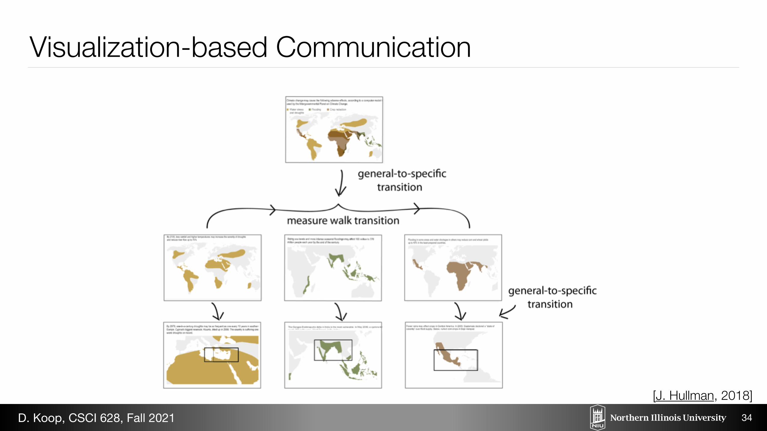
Fig. 1. Parallelism in sequencing in the NYTʼs “Copenhagen: Emis-sions, Treaties, and Impacts: Possible Impacts” interactive [3]. Three general-to-specific transitions detail three possible climate outcomes (drought, flooding, crop shortage), which at a higher level comprise a

measure walk sequence.

Visualization-based Communication

34



Design Studies• Studies of visualization in the world • Often involve collaboration with domain specialists • Specific problems in that domain that can provide lessons for other domains

as well

35



Formal Theories of Visualization• Grammar of Graphics • Discrete/Continuous Taxonomy • Algebraic Visualization

36



What should Visualization Research be about?• "[V]isualization is a method for contextualizing data, enabling people to apply

their prior experiences and perceptual and cognitive abilities to draw conclusions about phenomena in the real world" — J. Hullman

• Perception and cognition • Not only that Vis A is better than Vis B, but why

37



Visualization Research Boundaries?• Interactive illustration • Satellite imagery • Sketching and analogical reasoning • Understanding aesthetics independent of analytical utility • Tables • Uncertainty Vis: Worse than Nothing?

38



Grand Challenges• Amplifying human cognition in the exploration of data. - Data science - Explainable artificial intelligence - Information visualization is vital to successful outcomes for both topics.

• Improve storytelling capacity for the general public • Engage users to explore on their own • Support researchers in understanding causality • Shift from rationalism, which assumes that algorithms are the answer, to

empiricism, which assumes that continuous exploration, persistent questioning, and vigorous dialog will promote a deeper understanding of our world.

39



Shneiderman's Advice to a Ph.D. Student• "Start by working on a real problem—one that you have or that you get from

someone else. Working on real problems leads to better theories and better tools."

40



Documents

Visualization Research - faculty.cs.niu.edu