Cell Reports, Volume 18

Supplemental Information

Visualization of Chromatin Decompaction and Break

Site Extrusion as Predicted by Statistical

Polymer Modeling of Single-Locus Trajectories

Assaf Amitai, Andrew Seeber, Susan M. Gasser, and David Holcman

Supplementary Material

Visualization of chromatin decompaction and break site extrusion as predicted by statistical polymer modeling of single locus trajectories Amitai, Seeber, Gasser and Holcman Inventory 1 - Detailed Supplemental Experimental Procedures p 2 2 - Supplemental Tables p 12 Table S1: Strains used in this study p 12 A list of the yeast strains, index number and original citation. Table S2: HO endonuclease cutting efficiencies p 13 A list of the HO endonuclease cutting efficiencies for all experiments and number of independent trajectories/foci analyzed for each condition. Table S3: Parameters for self-avoiding polymers p 14 A table of the values used in self-avoiding polymer simulations. Table S4: Volumes of LacI-GFP Foci p 14 Volumes obtained by super resolution imaging and significance determined by a two tailed a Student’s t-test. 3 - Supplemental Figures p 15 Figure S1: Imaging regimes do not activate the DNA damage response, rel. to Figure 1. p 15 This figure shows that the imaging regimes used in the study do not activate a cell cycle arrest. Figure S2: Extracting values for the effective diffusion coefficient (Dc), rel. to Figure 1 p 16 Values obtained for the effective diffusion coefficient (Dc) from the same dataset as in Figure 1. Figure S3: Effect of an external force on locus motion, related to Figure 2 p 17 We show how a drift applied to a polymer causes α to increase, as does oscillatory forces. Increased amplitude or frequency of the force applied can lead to increased α. Figure S4: Depolymerization of actin cables by LatA at the concentration used in Figure 2 p 18 The effect of LatA on yeast actin is shown by staining for actin cables and immunoblotting. This important control shows that the LatA is working at the concentration used. Figure S5: Effect of LatA on spindle pole body and chromatin movement, related to Figure 2 p 19 Values for the statistical parameters after LatA treatment for the MAT locus and the spindle pole body are presented, with values extracted from MAT locus trajectories with LatA at ∆t=300ms. Figure S6: Trajectory parameters extracted from ARP8+ and arp8Δ cells, related to Figure 4 p 20 The three other parameters (Dc, Lc, Kc) extracted from trajectories in arp8Δ cells. Figure S7: Steady state configuration of a β-polymer with Lennard-Jones forces, rel. to Figure 4 p 20 This figure shows a β-polymer with Lennard-Jones forces applied under different values for β. Figure S8: Dynamic decondensation of a β-polymer, related to Figure 5 p 21 Here we show extrusion of a monomer within a β-polymer over time. Figure S9: Dynamics of rDNA locus before and after cut induction related to Figure 5 p 22 The values for the parameters not shown in Figure 5 before and after LatA treatment. Figure S10: Correlation between the statistical parameters, related to the Discussion p 23 The relationships between the four parameters as discussed in the main text. 4 - References p 25

2

1 - Detailed Supplemental Experimental Procedures

Yeast growth conditions and cleavage induction method

Yeast strains used in this study are in Table S1. Yeast cultures were grown at 30°C, and imaged

at 25°C. Strains were either W303 background or JKM179 as previously described (Dion et

al., 2012; van Attikum et al., 2007). The Ruby2 fluorophore plasmid was acquired from

Addgene (Lee et al., 2013). LatA and Nocodazole were dissolved in DMSO, and were added

1 h after galactose addition at a final concentration of 25µM and 50 µM respectively. Both

treated and control cultures were adjusted to 1% DMSO. For live cell imaging, 5 ml of YPAD

(2% Bactopeptone, 1% yeast extract, 0.01% adenine, 2% glucose) was inoculated and grown

over night. In the morning the culture was diluted to 2x106 cells per ml in synthetic complete

media containing 3% glycerol and 2% lactate (SCLG). The cells were then grown for a

minimum of 4 hours or until the culture doubled 1.5 times. The Gal1-10p driven HO gene was

induced for 2 h by adding galactose to the culture to a final concentration of 2%. These growth

conditions differ to those used previously for galactose induction (Horigome et al., 2015) where

a diluted overnight YPAD culture is allowed to grow for ~10 hours in SCLGg (containing

0.05% glucose), before addition of galactose. Cell growth conditions for 3D-SIM imaging were

similar to those used for live cell imaging except that YPLG (2% Bactopeptone, 1% yeast

extract, 3% glycerol and 2% lactate) media was used instead of synthetic complete media.

Before galactose addition the cells were synchronized in G1 phase by the addition of 1 µg/ml

alpha factor for 1.5 h. For S-phase cells, cultures were released from α-factor into media + 2%

galactose for 30 min.

DNA was extracted for quantitative PCR (QPCR) by spinning down 1 ml of cells and

resuspending them in 100 µl of 200 mM LiAc (lithium acetate) containing 1% SDS (sodium

dodecyl sulfate). The samples were incubated at 70 °C for 15 min after which 300 µl of 96%

ethanol was added. The samples were then vortexed briefly and centrifuged at maximum speed

for 3 minutes to collect DNA. The supernatant was removed and 100 µl of nuclease free water

was added. Cell debris was pelleted by a 1 min high speed spin at maximum speed and 0.5-1

µl of the supernatant was used in a QPCR reaction. This method has been tested for QPCR

(Looke et al., 2011). The efficiency of DSB induction was determined by QPCR with TaqMan

probes as previously described (van Attikum et al., 2007) and the results are in Table S2. QPCR

values were normalized to the SMC2 locus (van Attikum et al., 2007) and primer and probe

sequences are available on request.

3

We used the galactose inducible I-SceI-expressing strain (GA-6587 containing the I-SceI

expressing plasmid pWJ1108) with a cleavage consensus in the rDNA (Torres-Rosell et al.,

2007), because it was well characterized. In addition, the nucleolus was visualized in this strain

by transformation of cells with a plasmid containing NOP1-CFP (SG-3453). In Torres-Rosell

et al., the authors show that after 2h of cut induction (the conditions we use), 50% of I-SceI cut

loci move outside of the nucleolus and 40% move to its periphery. A minority (10%) remain

inside after I-SceI induction. Importantly, only ~10% I-SceI sites are found outside of the

nucleolus in cells without I-Sce1 induction.

Live cell microscopy

Live microscopy was done at 25°C on a Nikon Eclipse Ti microscope, two EM-CCD Cascade

II (Photometrics) cameras, an ASI MS-2000 Z-piezo stage and a PlanApo x100, NA 1.45 total

internal reflection fluorescence microscope oil objective and Visiview software. Fluorophores

were excited at 561 nm (Ruby2) and 491 nm (GFP), and emitted fluorescence was acquired

simultaneously on separate cameras (Semrock FF01-617/73-25 filter for mCherry/Ruby2 and

Semrock FF02-525/40-25 filter for GFP). Time-lapse series were streamed taking 8 optical

slices per stack either every 80 ms for 60 s or 300 ms for 120 s, with 10 ms and 30 ms exposure

times per slice respectively with laser powers set to ~7-12% for either laser line. Gain was set

to 800. Nuclear volumes are based on an average haploid nuclear radius of 0.9 µm. Time-lapse

image stacks were analyzed as in (Dion et al., 2012), using a custom made ImageJ (FIJI) plug-

in (Sage et al., 2005), to correct for translational movement and to extract locus coordinates.

Structured illumination microscopy (SIM) Structured illumination images were acquired at 23°C on a Zeiss Elyra S.1 microscope with a

Andor iXon 885 EM-CCD camera using a HR diode 488 nm 100nW solid state laser, BP 525-

580 + LP 750 filter and a PLAN-APOCHROMAT 63x N.A. 1.4 oil DIC objective lens. Cells

were first fixed in freshly dissolved paraformaldehyde (PFA) 4% w/v for 5 min, washed 3 times

in PBS and then attached glass slide using Concanavalin A. A thin SIM grade Zeiss 1.5 glass

coverslip was used while imaging. Cells were fully sectioned by 50 slices with 0.1 nm intervals

taken at 50 ms exposures per slice using 5 rotations of the illumination grid. Brightfield images

of the cells were also acquired using an X-Cite PC 120 EXFO Metal Halide lamp. Zen Black

was used to process the images using manual settings including Raw Scale. An automatic noise

filter was used within the range of -4 to -6. The pixel size of the images after processing is 39

nm. 3D stacks were segmented using Ilastik and the subsequent probability masks projected

onto the image using a custom Matlab script to determine the spot volumes. Volumes were

4

filtered to exclude spots smaller than 200 and greater than 3000 voxels.

Actin filament staining 10 µl of Rhodamine phalloidin (6.6 µm) was added to 100 µl of PFA fixed cells (4%

paraformaldehyde for 5 min) and stained overnight. After washing in PBS the cells were

imaged using SIM as above, with the 561 nm laser and appropriate emission filter. 60 z slices

were acquired with a 100 nm step size using 5 rotations of the structured illumination grid.

The same aliquot of fixed cells was used for an actin Western blot. Sample buffer + 0.1 M DTT

were added to the cells and they were heated to 95°C for 1 h to reverse crosslinking. Samples

were run on a 4-12% SDS-PAGE gel and blotted using a Transblot turbo machine. The

membrane was blocked in TENT (40 mM Tris-HCl (pH 7.5), 1mM EDTA (pH 8.0), 150 mM

NaCl and 0.05% Tween-20) + 5% milk for 1 h. Actin was stained with a mouse anti-actin

antibody (Millipore MAB1501, 1:10000) in TENT + 5% milk followed by a HRP conjugated

mouse secondary antibody (1:10000). Ponceau S staining revealed total protein content.

Selection of foci and extraction of parameters

Due to the linearity of the equations, the dynamics of a Rouse polymer can be studied by

projecting the equations on any axis. The parameters we calculated (Lc, α, kc, and Dc) can be

estimated separately in the projected equations. Because other motion such as nucleus

precession can influence the parameter estimation, we computed the anomalous α in both

spatial axes separately (αx and αy), as any additional motion of the nucleus can influence α

(Figure 2A). In Figure S3B, we show how the α estimate for a SPT of a Rouse polymer changes

when a drift is added. We find that drift increases α to 0.66 (intermediate time interval, red

line) from α= 0.5 (black line). Indeed, high values of α are the signature of an additive drift.

In the presented results, we consider the α best representing the system to be the smaller value

and thus consider that },{= yxMin ααα . In addition, we excluded nuclei containing aberrantly

large steps which are defined as steps ≥ 500 nm for the imaging regimes of Δt=80 ms or 300

ms, where a step is given by the difference |)()1)((| tktk cc ∆−∆+ RR . While α is estimated on a

single axis, Lc, kc and Dc are estimated using both the x and y axis.

Effect of an external force on locus motion We computed the anomalous exponent α (see below for derivation) from the projection of the

dynamics on each axis of an orthogonal frame. The value of α computed for each direction for

many cells, was often larger than 0.5 (Fig. 1). To interpret these values, we consider that an

5

additional force can be applied to the locus. We implemented this force using numerical

simulations in two conditions: either the force was deterministic (directed) or it was random.

We then computed the anomalous exponent α from the first six points of the time auto-

correlation function, power-law ( αtCtC ×=)( , where C is a constant).

An external deterministic force increases the anomalous exponent α A deterministic force acting on a polymer affects any monomer motion. In practice such added

motion can account for nuclear rotation, long time reorganization or simply measurement

artifacts. Using a Rouse polymer embedded into a constant drift field with amplitude

bD/0.2|=| v (see Fig. S3A), monomers are described by

𝑑𝑑𝑅𝑅𝒊𝒊,𝒏𝒏𝑑𝑑𝑑𝑑

= −𝐷𝐷𝛻𝛻𝑅𝑅𝒊𝒊,𝒏𝒏𝑈𝑈(𝑹𝑹) + √2𝐷𝐷𝑑𝑑𝑤𝑤𝒊𝒊,𝒏𝒏

𝑑𝑑𝑑𝑑, (1)

where

𝑈𝑈(𝑹𝑹) = 𝑈𝑈Rouse(𝑹𝑹1, . .𝑹𝑹𝑁𝑁) + 𝑈𝑈drift(𝑹𝑹1, . .𝑹𝑹𝑁𝑁), (2)

with

𝑈𝑈Rouse(𝑹𝑹1, . . . ,𝑹𝑹𝑁𝑁) =12𝜅𝜅�(𝑁𝑁−1

𝑖𝑖=1

𝑹𝑹𝑛𝑛+1 − 𝑹𝑹𝑛𝑛)2, (3)

where 𝜅𝜅 = 3𝑘𝑘𝐵𝐵𝑇𝑇𝑏𝑏2

, 𝑏𝑏 is the standard deviation of the bond length and

𝑈𝑈drift(𝑹𝑹1, . . . ,𝑹𝑹𝑁𝑁) = −�𝒗𝒗 ⋅ 𝑹𝑹𝑛𝑛𝐷𝐷

𝑛𝑛

. (4)

The anomalous exponent α is computed in intermediate time regime (Fig. S3A) and statistics

of the simulations with such drift reveals that α=0.66 (Fig. S3B) (compared to α=0.5 for a

Rouse polymer). Over longer periods of time, the motion of the center of mass becomes

ballistic. In summary, adding a deterministic drift to the motion of a polymer increases α,

providing an explanation for values scored 0.5> .

Oscillating forces on monomers increases the anomalous exponent To further evaluate the effect of external forces on a monomer motion, we now consider those

with oscillating properties (Fig. S3C), so that the total energy in eq. (1) is now

𝑈𝑈(𝑹𝑹1, . .𝑹𝑹𝑁𝑁) = 𝑈𝑈Rouse(𝑹𝑹1, . .𝑹𝑹𝑁𝑁) + 𝑈𝑈osc(𝑹𝑹1, . .𝑹𝑹𝑁𝑁), (5)

with

𝑈𝑈osc(𝑹𝑹1, . . . ,𝑹𝑹𝑁𝑁) = �(𝑛𝑛

𝑨𝑨 ⋅ 𝑹𝑹𝑛𝑛) sin (𝜔𝜔𝑑𝑑 + 𝜃𝜃𝑛𝑛), (6)

where ω,A are constants and the phases nθ can be chosen as follows. There are two extreme

6

cases: either all 0=nθ for Nn 1..= or )(0,2πθ U:n are random variables chosen

uniformly distributed. We observe that increasing the amplitude A or the frequency ω

increases the anomalous exponent value (Fig. S3D). For example, for 1=/= bkA T and

ω=b2/D, where nθ are randomly chosen, the anomalous exponent increases from 0.5=α

(Rouse) to 0.64. We conclude that any deterministic motion added on the DNA locus will

produce an increase of the anomalous exponent α .

Ghosh and Gov (Ghosh and Gov, 2014) use an alternative approach to model the effect of ATP-

dependent active fluctuations, by considering exponentially correlated colored noise acting on

the monomers of a semiflexible polymer. In this case the colored noise also resulted in

anomalous motion with an exponent much higher than the one obtained with a Gaussian noise

( 3/4=α for a semiflexible polymer). This result confirms that values of 0.5>α can be

explained by an external force component acting on chromatin and not simply reflect changes

in internal forces among monomers.

We note that the action of ATPase-driven motor proteins or of mechanical properties of the

nucleus can be modeled by adding local oscillatory forces on some monomers (Fig. S3C). By

increasing the magnitude of these oscillatory forces the α of monomers increases. For example,

for oscillatory forces with random phases acting on each of the monomers (force amplitude of

= / = 1TA k b and oscillation frequency ω=b2/D), the α computed from our numerical

simulations increases from 0.5 to 0.64 (Fig. S3D). Given that the impact of an oscillatory force

on chromatin depends on its intrinsic characteristic time (τ=2π/ ω), these effects could also

explain the changes in α values measured at different time intervals.

Implementing excluded volume interactions We used other polymer models than Rouse by adding interactions such as bending elasticity,

which accounts for the persistence length of the polymer and Lennard-Jones forces (LJ),

describing self-avoidance of each monomer pair. To account for the LJ forces, we use the

potential energy defined by

),,..(),..(=),..( 111 NLJNspringN UUU RRRRRR + (7)

where the spring potential is

1

21 , 1 0

=1

1( ,.. ) = (| | )2

N

spring N i ii

U lκ−

+ −∑R R r , (8)

7

where 0l is the equilibrium length of a bond, 2

0

3=ls

κ and 0l

s is the standard deviation of the

bond length. We chose the empirical relation 000.2= lsl . The Lennard-Jones potential is

),(=),..( ,,

,,1 ji

jiLJ

jijiNLJ UU rRR ∑

≠

(9)

with jiji RRr −=, and

≥

+

−

,2|<|for0

2||for4124

=)(1/6

,

1/6,

6

,

12

,,,

σ

σσσ

ji

jijijiji

jiLJU

r

rrrr (10)

where σ is the size of the monomer. With the choice σ2=0l , the springs which materialize

bonds, cannot cross each other in stochastic simulations using supplemental eq. 16 with

potential 2. We do not account here for bending elasticity. Finally, we used Euler’s scheme to

generate Brownian simulations (Schuss, 2009). At an impenetrable boundary, each rigid

monomer is reflected in the normal direction of the tangent plane.

Estimating the anomalous diffusion exponent α and the diffusion coefficient We computed the auto-correlation (AC) function or the MSD using the classical estimator

(Schuss, 2009)

2

=1

1( ) = ( ( ) ( )) 1.. 1,N qp

c c pkp

C t k t k t q t q NN q

−

∆ − ∆ + ∆ = −− ∑ R R (11)

where 𝑑𝑑 = 𝑞𝑞∆𝑑𝑑, is the time difference between the trajectory frames and pN is the number

of points in the trajectory. In many studies the AC function is referred to as the MSD function

(Dion et al., 2012; Mine-Hattab and Rothstein, 2012). The MSD is defined as the squared

displacement with respect to the initial trajectory position, averaged over time:

( )2MSD(t)= ( ) (0)c cR t R− .

For short times, )(tC or MSD(t) increases as a power law

( ) ,C t Ctα≈ (12)

where 0>C . To extract the coefficient α, we computed )(tC from empirical trajectories and

8

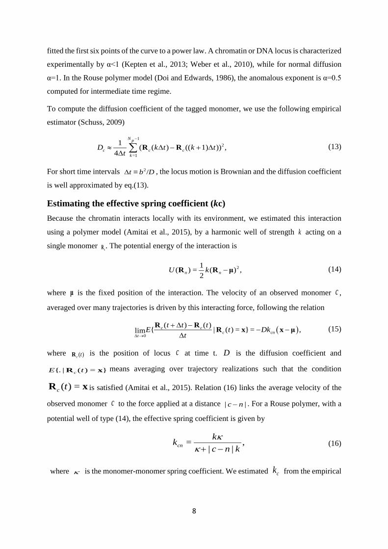
fitted the first six points of the curve to a power law. A chromatin or DNA locus is characterized

experimentally by α<1 (Kepten et al., 2013; Weber et al., 2010), while for normal diffusion

α=1. In the Rouse polymer model (Doi and Edwards, 1986), the anomalous exponent is α=0.5

computed for intermediate time regime.

To compute the diffusion coefficient of the tagged monomer, we use the following empirical

estimator (Schuss, 2009)

1

2

=1

1 ( ( ) (( 1) )) ,4

N p

c c ck

D k t k tt

−

≈ ∆ − + ∆∆ ∑ R R (13)

For short time intervals Dbt /2=∆ , the locus motion is Brownian and the diffusion coefficient

is well approximated by eq.(13).

Estimating the effective spring coefficient (kc) Because the chromatin interacts locally with its environment, we estimated this interaction

using a polymer model (Amitai et al., 2015), by a harmonic well of strength k acting on a

single monomer nR . The potential energy of the interaction is

,)(21=)( 2μRR −nn kU (14)

where μ is the fixed position of the interaction. The velocity of an observed monomer c ,

averaged over many trajectories is driven by this interacting force, following the relation

( )0

( ) ( ){ | ( ) = } = ,lim c cc cn

t

t t tE t Dkt∆ →

+ ∆ −− −

∆R R R x x μ (15)

where )(tcR is the position of locus c at time t. D is the diffusion coefficient and

{. | ( ) = }cE tR x means averaging over trajectory realizations such that the condition

( ) =c tR x is satisfied (Amitai et al., 2015). Relation (16) links the average velocity of the

observed monomer c to the force applied at a distance || nc − . For a Rouse polymer, with a

potential well of type (14), the effective spring coefficient is given by

,||

=knc

kkcn −+κκ

(16)

where κ is the monomer-monomer spring coefficient. We estimated ck from the empirical

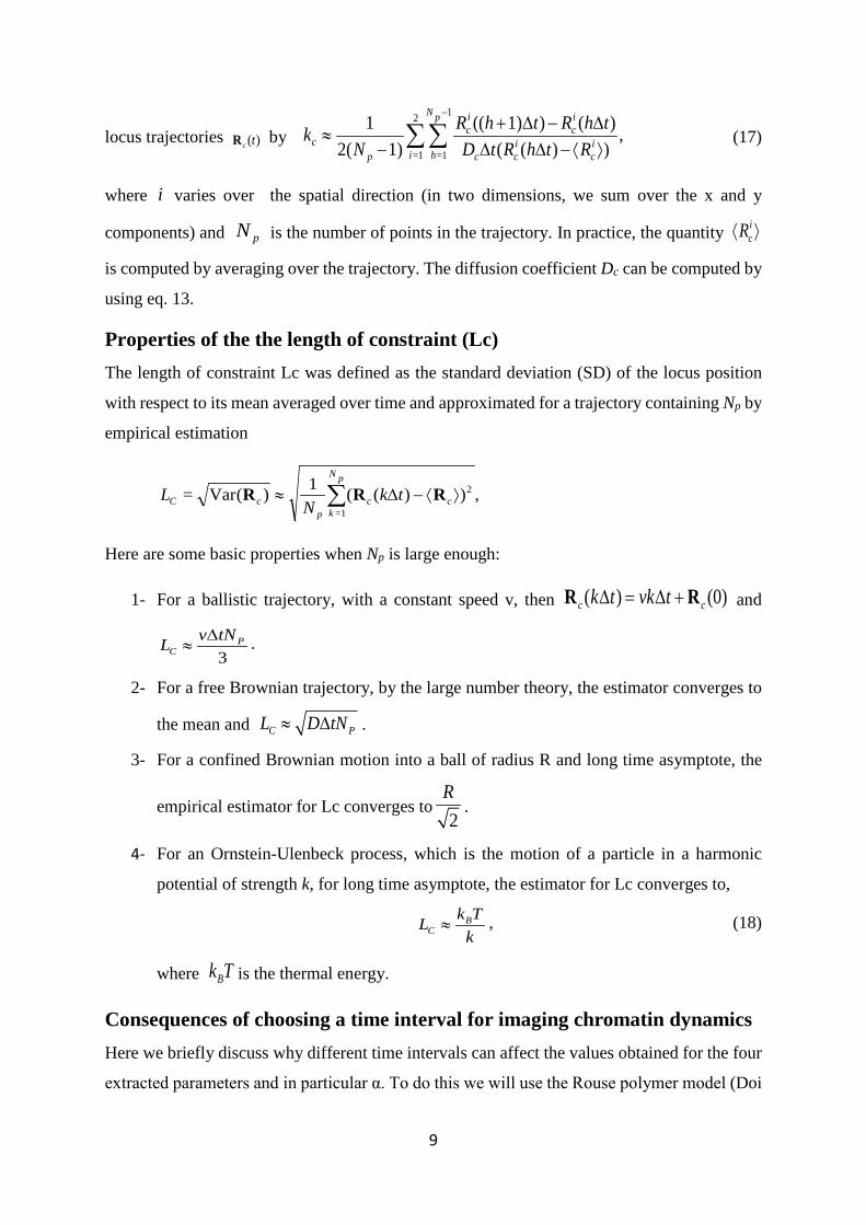
9

locus trajectories )(tcR by ,))(()()1)((

1)2(1

1

1=

2

1= ⟩⟨−∆∆∆−∆+

−≈ ∑∑

−

ic

icc

ic

ic

pN

hipc RthRtD

thRthRN

k (17)

where i varies over the spatial direction (in two dimensions, we sum over the x and y

components) and pN is the number of points in the trajectory. In practice, the quantity ⟩⟨ icR

is computed by averaging over the trajectory. The diffusion coefficient Dc can be computed by

using eq. 13.

Properties of the the length of constraint (Lc) The length of constraint Lc was defined as the standard deviation (SD) of the locus position

with respect to its mean averaged over time and approximated for a trajectory containing Np by

empirical estimation

,))((1)(Var= 2

=1⟩⟨−∆≈ ∑ cc

pN

kpcC tk

NL RRR

Here are some basic properties when Np is large enough:

1- For a ballistic trajectory, with a constant speed v, then ( ) (0)c ck t vk t∆ = ∆ +R R and

3P

Cv tNL ∆

≈ .

2- For a free Brownian trajectory, by the large number theory, the estimator converges to

the mean and C PL D tN≈ ∆ .

3- For a confined Brownian motion into a ball of radius R and long time asymptote, the

empirical estimator for Lc converges to2

R.

4- For an Ornstein-Ulenbeck process, which is the motion of a particle in a harmonic

potential of strength k, for long time asymptote, the estimator for Lc converges to,

BC

k TLk

≈ , (18)

where Bk T is the thermal energy.

Consequences of choosing a time interval for imaging chromatin dynamics

Here we briefly discuss why different time intervals can affect the values obtained for the four

extracted parameters and in particular α. To do this we will use the Rouse polymer model (Doi

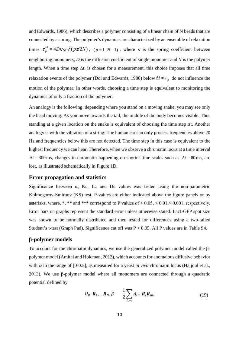
10

and Edwards, 1986), which describes a polymer consisting of a linear chain of N beads that are

connected by a spring. The polymer’s dynamics are characterized by an ensemble of relaxation

times )/2(sin4= 21 NpDp πκτ − , 1)1..=( −Np , where κ is the spring coefficient between

neighboring monomers, D is the diffusion coefficient of single monomer and N is the polymer

length. When a time step ∆t, is chosen for a measurement, this choice imposes that all time

relaxation events of the polymer (Doi and Edwards, 1986) below pt τ≈∆ do not influence the

motion of the polymer. In other words, choosing a time step is equivalent to monitoring the

dynamics of only a fraction of the polymer.

An analogy is the following: depending where you stand on a moving snake, you may see only

the head moving. As you move towards the tail, the middle of the body becomes visible. Thus

standing at a given location on the snake is equivalent of choosing the time step ∆t. Another

analogy is with the vibration of a string: The human ear can only process frequencies above 20

Hz and frequencies below this are not detected. The time step in this case is equivalent to the

highest frequency we can hear. Therefore, when we observe a chromatin locus at a time interval

300=t∆ ms, changes in chromatin happening on shorter time scales such as 80=t∆ ms, are

lost, as illustrated schematically in Figure 1D.

Error propagation and statistics Significance between α, Kc, Lc and Dc values was tested using the non-parametric

Kolmogorov-Smirnov (KS) test. P-values are either indicated above the figure panels or by

asterisks, where, *, ** and *** correspond to P values of ≤ 0.05, ≤ 0.01,≤ 0.001, respectively.

Error bars on graphs represent the standard error unless otherwise stated. LacI-GFP spot size

was shown to be normally distributed and then tested for differences using a two-tailed

Student’s t-test (Graph Pad). Significance cut off was P < 0.05. All P values are in Table S4.

β-polymer models To account for the chromatin dynamics, we use the generalized polymer model called the β-

polymer model (Amitai and Holcman, 2013), which accounts for anomalous diffusive behavior

with α in the range of [0-0.5], as measured for a yeast in vivo chromatin locus (Hajjoul et al.,

2013). We use β-polymer model where all monomers are connected through a quadratic

potential defined by

𝑈𝑈𝛽𝛽(𝑹𝑹1, . .𝑹𝑹𝑁𝑁 ,𝛽𝛽) =12�𝐴𝐴𝑙𝑙𝑙𝑙𝑙𝑙,𝑙𝑙

𝑹𝑹𝑙𝑙𝑹𝑹𝑙𝑙, (19)

11

with coefficients

21-mcos

21-lcos

2sin24=~=

1

1=

1

1=,

∑∑

−−

Np

Np

Np

NA

N

p

mp

lpp

N

pml

πππκαακ β (20)

and

�̃�𝜅𝑝𝑝 = 4𝜅𝜅 sin𝛽𝛽�𝑝𝑝𝑝𝑝2𝑁𝑁

�  for 𝑝𝑝 = 0. .𝑁𝑁 − 1. (21)

In such a model, the strength of interaction mlA , decays with the distance || ml − along the

chain. By definition, 1<β<2 (Amitai and Holcman, 2013) and the Rouse polymer is recovered

for 2=β , for which only nearest neighbors are connected.

12

2 - Supplemental Tables

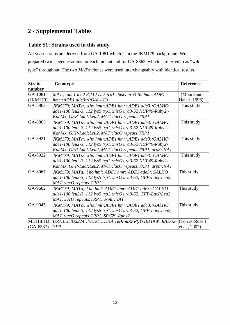
Table S1: Strains used in this study All yeast strains are derived from GA-1081 which is in the JKM179 background. We

prepared two isogenic strains for each mutant and for GA-8862, which is referred to as “wild-

type” throughout. The two MATα clones were used interchangeably with identical results.

Strain number

Genotype Reference

GA-1081 (JKM179)

MATα ade1 leu2-3,112 lys5 trp1::hisG ura3-52 hml::ADE1 hmr::ADE1 ade3::PGAL-HO

(Moore and Haber, 1996)

GA-8862 JKM179; MATα, ∆ho hml::ADE1 hmr::ADE1 ade3::GALHO ade1-100 leu2-3, 112 lys5 trp1::hisG ura3-52 NUP49-Ruby2 -KanMx, GFP-LacI:Leu2, MAT::lacO repeats:TRP1

This study

GA-8863 JKM179; MATα, ∆ho hml::ADE1 hmr::ADE1 ade3::GALHO ade1-100 leu2-3, 112 lys5 trp1::hisG ura3-52 NUP49-Ruby2- KanMx, GFP-LacI:Leu2, MAT::lacO repeats:TRP1

This study

GA-8921 JKM179; MATα, ∆ho hml::ADE1 hmr::ADE1 ade3::GALHO ade1-100 leu2-3, 112 lys5 trp1::hisG ura3-52 NUP49-Ruby2- KanMx, GFP-LacI:Leu2, MAT::lacO repeats:TRP1, arp8::NAT

This study

GA-8922 JKM179; MATα, ∆ho hml::ADE1 hmr::ADE1 ade3::GALHO ade1-100 leu2-3, 112 lys5 trp1::hisG ura3-52 NUP49-Ruby2- KanMx, GFP-LacI:Leu2, MAT::lacO repeats:TRP1, arp8::NAT

This study

GA-8067 JKM179; MATa, ∆ho hml::ADE1 hmr::ADE1 ade3::GALHO ade1-100 leu2-3, 112 lys5 trp1::hisG ura3-52, GFP-LacI:Leu2, MAT::lacO repeats:TRP1

This study

GA-9602 JKM179; MATa, ∆ho hml::ADE1 hmr::ADE1 ade3::GALHO ade1-100 leu2-3, 112 lys5 trp1::hisG ura3-52, GFP-LacI:Leu2, MAT::lacO repeats:TRP1, arp8::NAT

This study

GA-9045 JKM179; MATα, ∆ho hml::ADE1 hmr::ADE1 ade3::GALHO ade1-100 leu2-3, 112 lys5 trp1::hisG ura3-52, GFP-LacI:Leu2, MAT::lacO repeats:TRP1, SPC29-Ruby2

This study

ML118-1D (GA-6587)

URA3::tetOx224::I-Sce1::rDNA TetR-mRFP(iYGL119W) RAD52-YFP

(Torres-Rosell et al., 2007)

13

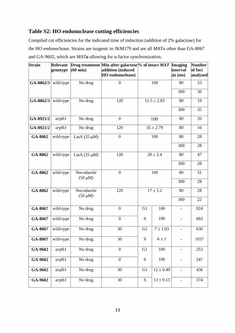
Table S2: HO endonuclease cutting efficiencies Compiled cut efficiencies for the indicated time of induction (addition of 2% galactose) for

the HO endonuclease. Strains are isogenic to JKM179 and are all MATα other than GA-8067

and GA-9602, which are MATa allowing for α-factor synchronization.

Strain

Relevant genotype

Drug treatment (60 min)

Min after galactose addition (induced HO endonuclease)

% of intact MAT Imaging interval Δt (ms)

Number of foci analyzed

GA-8862/3 wild-type No drug 0 100 80 33

300 30

GA-8862/3 wild-type No drug 120 11.5 ± 2.83 80 19

300 35

GA-8921/2 arp8Δ No drug 0 100 80 20

GA-8921/2 arp8Δ No drug 120 35 ± 2.79 80 16

GA-8862

wild-type LatA (25 µM) 0 100 80 28

300 28

GA-8862 wild-type LatA (25 µM) 120 20 ± 2.4 80 47

300 28

GA-8862

wild-type Nocodazole (50 µM)

0 100 80 31

300 28

GA-8862

wild-type Nocodazole (50 µM)

120 17 ± 1.2 80 28

300 22

GA-8067 wild-type No drug 0 G1 100

100

- 924

GA-8067 wild-type No drug 0 S - 683

GA-8067 wild-type No drug 30 G1 7 ± 1.03

6 ± 1

- 630

GA-8067 wild-type No drug 30 S - 1037

GA-9602 arp8Δ No drug 0 G1 100

100

- 253

GA-9602 arp8Δ No drug 0 S - 247

GA-9602 arp8Δ No drug 30 G1 12 ± 0.49

13 ± 0.13

- 436

GA-9602 arp8Δ No drug 30 S - 374

14

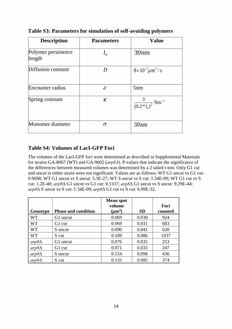
Table S3: Parameters for simulation of self-avoiding polymers

Description Parameters Value

Polymer persistence length

0l 30nm

Diffusion constant D 3 28 10 m / sµ−×

Encounter radius ε 5nm

Spring constant κ 12

0

3 Nm(0.2* )l

−

Monomer diameter σ 30nm

Table S4: Volumes of LacI-GFP Foci The volumes of the LacI-GFP foci were determined as described in Supplemental Materials for strains GA-8067 (WT) and GA-9602 (arp8Δ). P-values that indicate the significance of the differences between measured volumes was determined by a 2 tailed t-test. Only G1 cut and uncut in either strain were not significant. Values are as follows: WT G1 uncut vs G1 cut: 0.9698; WT G1 uncut vs S uncut: 5.3E-27; WT S uncut vs S cut: 1.34E-09; WT G1 cut vs S cut: 1.2E-40; arp8∆ G1 uncut vs G1 cut: 0.1337; arp8∆ G1 uncut vs S uncut: 9.29E-44; arp8∆ S uncut vs S cut: 1.34E-09; arp8∆ G1 cut vs S cut: 6.99E-32.

Genotype Phase and condition

Mean spot volume (µm3) SD

Foci counted

WT G1 uncut 0.069 0.030 924 WT G1 cut 0.069 0.031 683 WT S uncut 0.090 0.041 630 WT S cut 0.109 0.086 1037 arp8∆ G1 uncut 0.076 0.035 253 arp8∆ G1 cut 0.071 0.033 247 arp8∆ S uncut 0.154 0.098 436 arp8∆ S cut 0.133 0.085 374

15

3 - Supplemental Figures

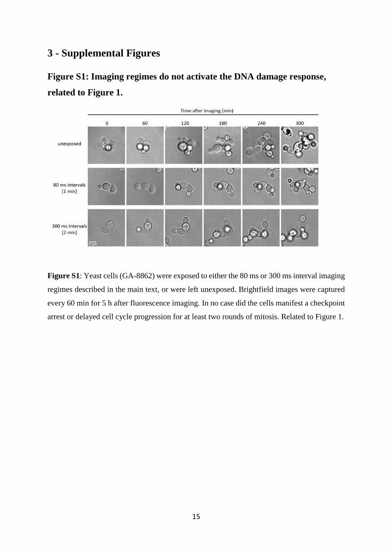
Figure S1: Imaging regimes do not activate the DNA damage response,

related to Figure 1.

Figure S1: Yeast cells (GA-8862) were exposed to either the 80 ms or 300 ms interval imaging

regimes described in the main text, or were left unexposed. Brightfield images were captured

every 60 min for 5 h after fluorescence imaging. In no case did the cells manifest a checkpoint

arrest or delayed cell cycle progression for at least two rounds of mitosis. Related to Figure 1.

16

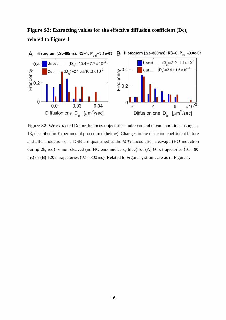
Figure S2: Extracting values for the effective diffusion coefficient (Dc),

related to Figure 1

Figure S2: We extracted Dc for the locus trajectories under cut and uncut conditions using eq.

13, described in Experimental procedures (below). Changes in the diffusion coefficient before

and after induction of a DSB are quantified at the MAT locus after cleavage (HO induction

during 2h, red) or non-cleaved (no HO endonuclease, blue) for (A) 60 s trajectories ( 80=t∆

ms) or (B) 120 s trajectories ( 300=t∆ ms). Related to Figure 1; strains are as in Figure 1.

17

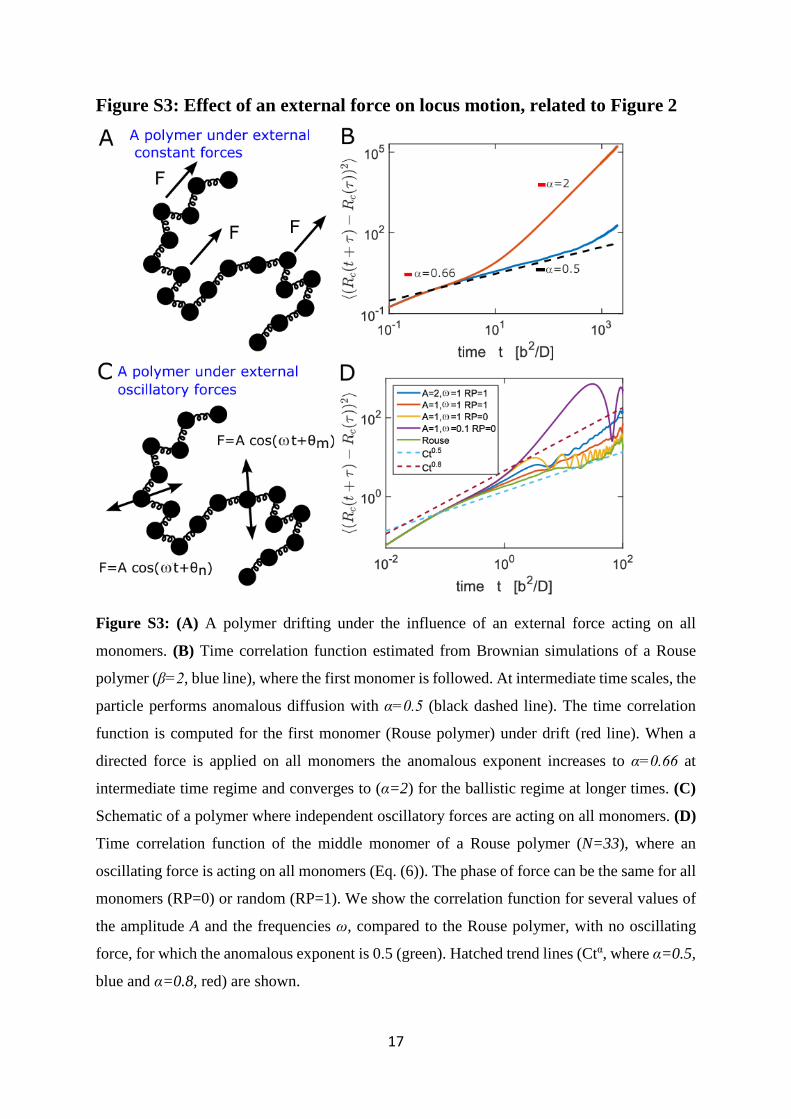
Figure S3: Effect of an external force on locus motion, related to Figure 2

Figure S3: (A) A polymer drifting under the influence of an external force acting on all

monomers. (B) Time correlation function estimated from Brownian simulations of a Rouse

polymer (β=2, blue line), where the first monomer is followed. At intermediate time scales, the

particle performs anomalous diffusion with α=0.5 (black dashed line). The time correlation

function is computed for the first monomer (Rouse polymer) under drift (red line). When a

directed force is applied on all monomers the anomalous exponent increases to α=0.66 at

intermediate time regime and converges to (α=2) for the ballistic regime at longer times. (C)

Schematic of a polymer where independent oscillatory forces are acting on all monomers. (D)

Time correlation function of the middle monomer of a Rouse polymer (N=33), where an

oscillating force is acting on all monomers (Eq. (6)). The phase of force can be the same for all

monomers (RP=0) or random (RP=1). We show the correlation function for several values of

the amplitude A and the frequencies ω, compared to the Rouse polymer, with no oscillating

force, for which the anomalous exponent is 0.5 (green). Hatched trend lines (Ctα, where α=0.5,

blue and α=0.8, red) are shown.

18

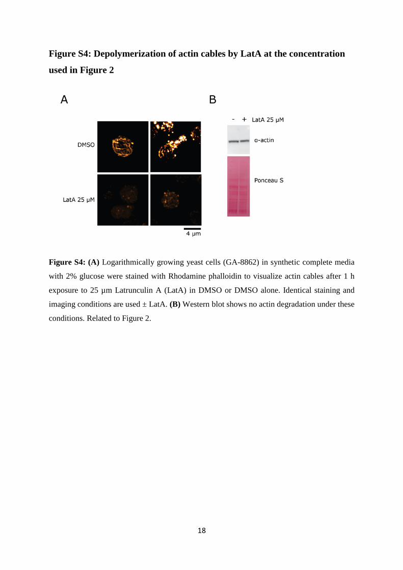
Figure S4: Depolymerization of actin cables by LatA at the concentration

used in Figure 2

Figure S4: (A) Logarithmically growing yeast cells (GA-8862) in synthetic complete media

with 2% glucose were stained with Rhodamine phalloidin to visualize actin cables after 1 h

exposure to 25 µm Latrunculin A (LatA) in DMSO or DMSO alone. Identical staining and

imaging conditions are used ± LatA. (B) Western blot shows no actin degradation under these

conditions. Related to Figure 2.

19

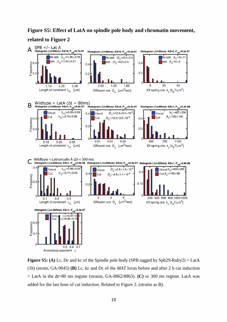
Figure S5: Effect of LatA on spindle pole body and chromatin movement,

related to Figure 2

Figure S5: (A) Lc, Dc and kc of the Spindle pole body (SPB tagged by Spb29-Ruby2) + LatA

(1h) (strain, GA-9045) (B) Lc, kc and Dc of the MAT locus before and after 2 h cut induction

+ LatA in the Δt=80 ms regime (strains, GA-8862/8863). (C) or 300 ms regime. LatA was

added for the last hour of cut induction. Related to Figure 2. (strains as B).

20

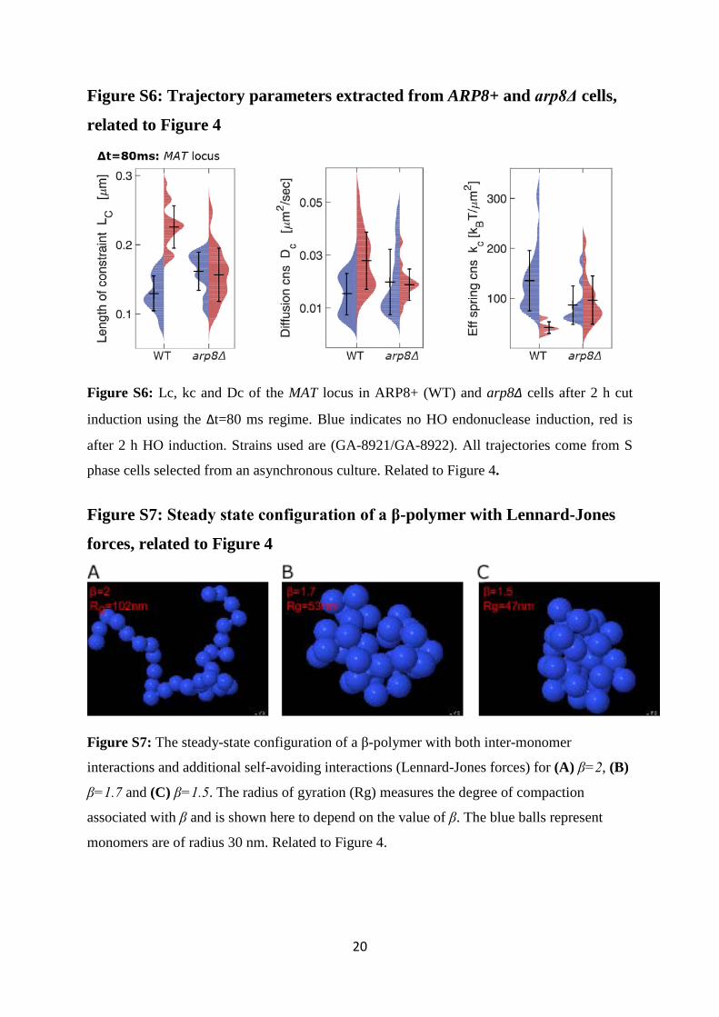
Figure S6: Trajectory parameters extracted from ARP8+ and arp8Δ cells,

related to Figure 4

Figure S6: Lc, kc and Dc of the MAT locus in ARP8+ (WT) and arp8Δ cells after 2 h cut

induction using the Δt=80 ms regime. Blue indicates no HO endonuclease induction, red is

after 2 h HO induction. Strains used are (GA-8921/GA-8922). All trajectories come from S

phase cells selected from an asynchronous culture. Related to Figure 4.

Figure S7: Steady state configuration of a β-polymer with Lennard-Jones

forces, related to Figure 4

Figure S7: The steady-state configuration of a β-polymer with both inter-monomer

interactions and additional self-avoiding interactions (Lennard-Jones forces) for (A) β=2, (B)

β=1.7 and (C) β=1.5. The radius of gyration (Rg) measures the degree of compaction

associated with β and is shown here to depend on the value of β. The blue balls represent

monomers are of radius 30 nm. Related to Figure 4.

21

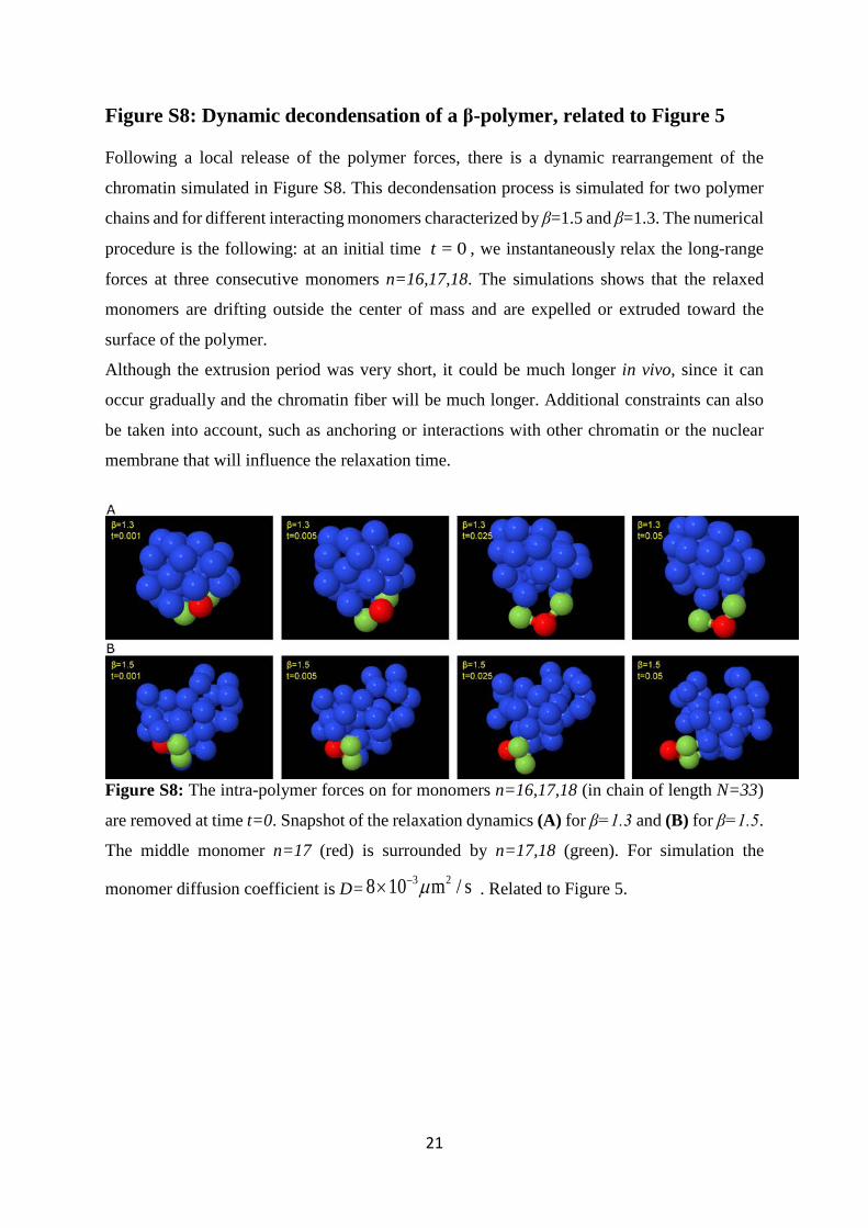
Figure S8: Dynamic decondensation of a β-polymer, related to Figure 5

Following a local release of the polymer forces, there is a dynamic rearrangement of the

chromatin simulated in Figure S8. This decondensation process is simulated for two polymer

chains and for different interacting monomers characterized by β=1.5 and β=1.3. The numerical

procedure is the following: at an initial time 0=t , we instantaneously relax the long-range

forces at three consecutive monomers n=16,17,18. The simulations shows that the relaxed

monomers are drifting outside the center of mass and are expelled or extruded toward the

surface of the polymer.

Although the extrusion period was very short, it could be much longer in vivo, since it can

occur gradually and the chromatin fiber will be much longer. Additional constraints can also

be taken into account, such as anchoring or interactions with other chromatin or the nuclear

membrane that will influence the relaxation time.

Figure S8: The intra-polymer forces on for monomers n=16,17,18 (in chain of length N=33)

are removed at time t=0. Snapshot of the relaxation dynamics (A) for β=1.3 and (B) for β=1.5.

The middle monomer n=17 (red) is surrounded by n=17,18 (green). For simulation the

monomer diffusion coefficient is D= 3 28 10 m / sµ−× . Related to Figure 5.

22

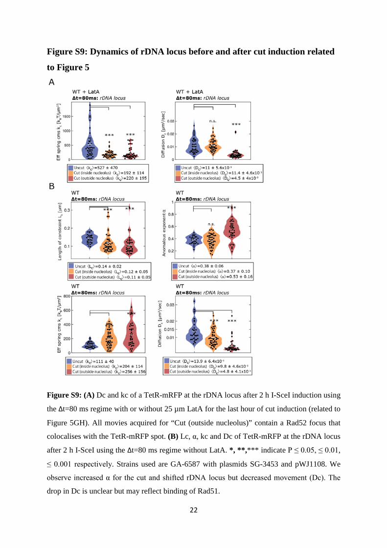
Figure S9: Dynamics of rDNA locus before and after cut induction related

to Figure 5

Figure S9: (A) Dc and kc of a TetR-mRFP at the rDNA locus after 2 h I-SceI induction using

the Δt=80 ms regime with or without 25 µm LatA for the last hour of cut induction (related to

Figure 5GH). All movies acquired for “Cut (outside nucleolus)” contain a Rad52 focus that

colocalises with the TetR-mRFP spot. (B) Lc, α, kc and Dc of TetR-mRFP at the rDNA locus

after 2 h I-SceI using the Δt=80 ms regime without LatA. *, **,*** indicate P ≤ 0.05, ≤ 0.01,

≤ 0.001 respectively. Strains used are GA-6587 with plasmids SG-3453 and pWJ1108. We

observe increased α for the cut and shifted rDNA locus but decreased movement (Dc). The

drop in Dc is unclear but may reflect binding of Rad51.

23

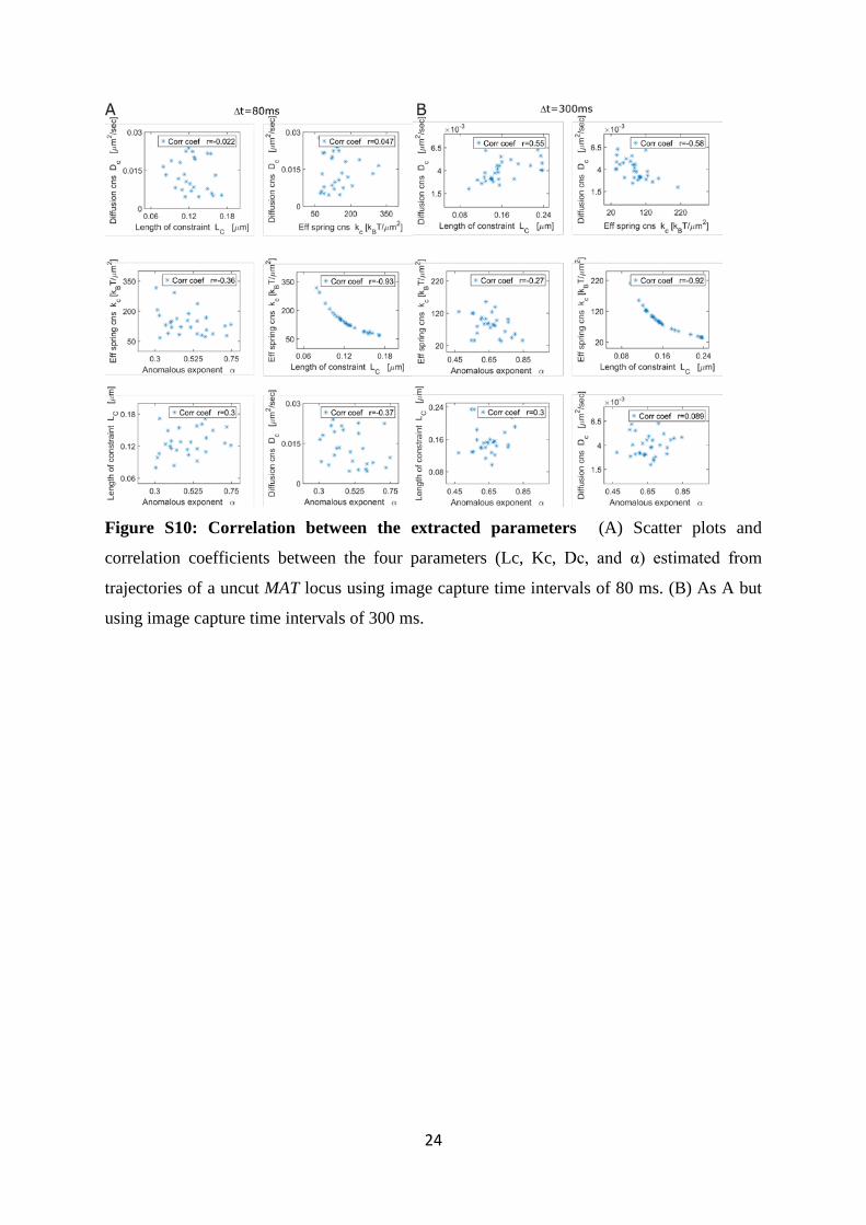
Figure S10: Correlation between the statistical parameters, related to the

Discussion

In this section we clarify the relationship between the 4 estimated parameters (Lc, Kc, Dc, and

α). Kc is computed from the first statistical moment of the displacement eq. (15 SI). It is

independent of α and Dc which are rather computed from the second moment of the

displacement, supplemental eqs. 11, 12 and 13. These estimators (first moment vs. second

moment) are expected to be independent. We confirm this by comparing the parameters

computed for an uncut MAT locus at ∆t =80ms and ∆t =300ms (see Figure S10AB). When

∆t=300ms the correlation coefficient between Lc and Dc is larger. While for ∆t=80ms the value

of the correlation coefficients of Lc with α and Dc is small.

When the confinement of a chromatin locus is driven by a tethering force, the length of

confinement Lc is inversely proportionally to the constant Kc as shown in equation 18 and

Figures S10AB, and Amitai et al., 2015. For other types of motion, this relationship is not

necessarily the same, as explained in the supplemental section, “Properties of the the length of

constraint (Lc)”. The algebraic relationship we have observed indicates that confinement of

this locus arises from a tethering force and not necessarily crowding. Moreover, the information

contained in α is different from the one in Dc. α has no dimension and it is obtained by fitting

the correlation function by a power law ( ) ,C t Ctα≈ as described above in the main text. The

effective diffusion coefficient has the physical units of µm2/s and is computed from

supplemental eq. 15. We confirm that α and Dc are uncorrelated (Figure S10AB). In the context

of the β-polymer model, α reflects the level of chromatin condensation.

In summary, the four parameters are computed from the first and second statistical moments

of the displacement. There are in general not redundant and provide independent information

about the dynamics of the underlying physical process that has generated the single particle

trajectories. The numerical code to compute the four parameters is accessible at

http://bionewmetrics.org/ in the “Nuclear Organization section” or

https://amitaiassaf.github.io/.

24

Figure S10: Correlation between the extracted parameters (A) Scatter plots and

correlation coefficients between the four parameters (Lc, Kc, Dc, and α) estimated from

trajectories of a uncut MAT locus using image capture time intervals of 80 ms. (B) As A but

using image capture time intervals of 300 ms.

25

4 - References

Amitai, A., and Holcman, D. (2013). Polymer model with long-range interactions: analysis and applications to the chromatin structure. Phys Rev E Stat Nonlin Soft Matter Phys 88, 052604.

Amitai, A., Toulouze, M., Dubrana, K., and Holcman, D. (2015). Analysis of Single Locus Trajec-tories for Extracting In Vivo Chromatin Tethering Interactions. PLoS Comp Biol 11, e1004433.

Dion, V., Kalck, V., Horigome, C., Towbin, B.D., and Gasser, S.M. (2012). Increased mobility of double-strand breaks requires Mec1, Rad9 and the homologous recombination machinery. Nature Cell Biology 14, 502-U221.

Doi, M., and Edwards, S.F. (1986). The Theory of Polymer Dynamics. Oxford: Clarendon Press.

Ghosh, A., and Gov, N.S. (2014). Dynamics of active semiflexible polymers. Biophys J 107, 1065-1073.

Hajjoul, H., Mathon, J., Ranchon, H., Goiffon, I., Mozziconacci, J., Albert, B., Carrivain, P., Victor, J.-M., Gadal, O., and Bystricky, K. (2013). High-throughput chromatin motion tracking in living yeast reveals the flexibility of the fiber throughout the genome. Genome research 23, 1829-1838.

Horigome, C., Dion, V., Seeber, A., Gehlen, L.R., and Gasser, S.M. (2015). Visualizing the spatiotemporal dynamics of DNA damage in budding yeast. Methods in molecular biology (Clifton, NJ) 1292, 77-96.

Kepten, E., Bronshtein, I., and Garini, Y. (2013). Improved estimation of anomalous diffusion exponents in single-particle tracking experiments. Phys Rev E Stat Nonlin Soft Matter Phys 87, 052713.

Lee, S., Lim, W.A., and Thorn, K.S. (2013). Improved blue, green, and red fluorescent protein tagging vectors for S. cerevisiae. PLoS One 8, e67902.

Looke, M., Kristjuhan, K., and Kristjuhan, A. (2011). Extraction of genomic DNA from yeasts for PCR-based applications. Biotechniques 50, 325-328.

Mine-Hattab, J., and Rothstein, R. (2012). Increased chromosome mobility facilitates homology search during recombination. Nat Cell Biol 14, 510-517.

Moore, J.K., and Haber, J.E. (1996). Cell cycle and genetic requirements of two pathways of nonhomologous end-joining repair of double-strand breaks in Saccharomyces cerevisiae. Mol Cell Biol 16, 2164-2173.

Sage, D., Neumann, F.R., Hediger, F., Gasser, S.M., and Unser, M. (2005). Automatic tracking of individual fluorescence particles: application to the study of chromosome dynamics. IEEE Trans Image Process 14, 1372-1383.

Schuss, Z. (2009). Diffusion and Stochastic Processes. An Analytical Approach. Springer-Verlag, New York, NY.

Torres-Rosell, J., Sunjevaric, I., De Piccoli, G., Sacher, M., Eckert-Boulet, N., Reid, R., Jentsch, S., Rothstein, R., Aragon, L., and Lisby, M. (2007). The Smc5-Smc6 complex and SUMO modification of Rad52 regulates recombinational repair at the ribosomal gene locus. Nat Cell Biol 9, 923-931.

van Attikum, H., Fritsch, O., and Gasser, S.M. (2007). Distinct roles for SWR1 and INO80 chromatin remodeling complexes at chromosomal double-strand breaks. Embo J 26, 4113-4125.

Weber, S.C., Theriot, J.A., and Spakowitz, A.J. (2010). Subdiffusive motion of a polymer composed of subdiffusive monomers. Phys Rev E Stat Nonlin Soft Matter Phys 82, 011913.