Visualization of Airfoil Boundary Layer by Infrared - QIRT

Visualization of Airfoil Boundary Layer by Infrared Thermography to Determine Influence of Roughness-Due-to-Insect

by J. Kuklova*, L. Popelka**, N. Souckova*** and T. Vitu****

*Dept. of Applied Mathematics, CTU in Prague – Faculty of Transportation Sciences, Konviktska 20, Prague 1, Czech Republic, [email protected]

**Institute of Thermomechanics, Academy of Sciences of the Czech Republic, Dolejskova 5, Prague 8, Czech Republic, [email protected]

***Institute of Thermomechanics, Academy of Sciences of the Czech Republic, Dolejskova 5, Prague 8, Czech Republic, [email protected]

****Dept. of Applied Mathematics, CTU in Prague – Faculty of Transportation Sciences, Konviktska 20, Prague 1, Czech Republic, [email protected]

Abstract

Flow visualization techniques often enable the first insight into the investigated problem. Generally, the particle image velocimetry, smoke-wire, tuft filaments and oil-flow visualization techniques are used for wind-tunnel investigation. Considering the phenomenon of boundary layer separation bubble related to the low-Reynolds number’s transition, these methods face several difficulties mainly with imposed influence to the sensitive flow mechanism. Infrared imaging allowing non-invasive visualization of the afore-mentioned investigations is one of the techniques currently undergoing further promising development in terms of resolution, device size, and price. In the presented paper, the focus was placed on validation of the infrared imaging as a standard visualization technique for wind-tunnel investigation of boundary layer development along an airfoil and its usage for roughness-due-to-insect investigation.

1. Introduction

Infrared thermography has been used as a visualization technique for more than two decades in both in-flight and wind-tunnel experiments [1]. Unfortunately, it has not expanded and traditional techniques as smoke-wire or oil-flow visualization are preferably used. This trend is usually observed given that the high-sensitivity infrared systems have been costly until recently.

Nevertheless, the main advantage of visualization by infrared thermography is its non-invasive character. Neither airflow, nor airfoil surface are not affected by any external matter. Belong this case, it appears as an ideal visualization method for a roughness-due-to-insect study where the insect elements represent slight interference in the airflow and another invasive visualization would be hard to apply.

In our previous investigation, the visualization technique was thoroughly studied [3], afterwards, it was applied in complex investigation of sailplanes [4], and used as a support for investigation of passive flow control devices [5].

The present paper is divided into three main parts. The first part provides the theoretical background of the visualization method. Then, practical experiments and a numerical approach are presented and compared to provide verification of introduced visualization method. The last part finally presents the systematic investigation of roughness-due-to-insect.

2. Theoretical background

The theoretical background consists of two main parts that briefly explain principles of airflow visualization by infrared thermography. While the first part deals with general principles of infrared thermography that are applicable for all related tasks, the second part is focused particularly on airfoil boundary layer visualization by infrared thermography. The first part also introduces the infrared camera that was used for all the measurements presented in this study.

2.1. Infrared Thermography

Infrared thermography is based on assumption that all bodies with non-zero thermodynamic temperature radiate electromagnetic energy in the infrared spectral band. An infrared system then detects the energy and converts it into an electronic signal. Such systems that are also able to display temperature patterns (thermograms) corresponding to surface temperatures pertain to the general category of infrared thermographic systems.

The measurement principle is based on the broadly known Plank law which gives the spectral radiant emittance Hλ of blackbody as a function of wavelength λ (or frequency) and thermodynamic temperature T. An adjustment for real

11th International Conference on

Quantitative InfraRed Thermography

http://dx.doi.org/10.21611/qirt.2012.332

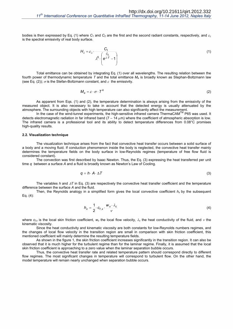
bodies is then expressed by Eq. (1) where C1 and C2 are the first and the second radiant constants, respectively, and ελ is the spectral emissivity of real body surface.

⎟⎟

⎠

⎞

⎜⎜

⎝

⎛−⋅

⋅=⋅ 12

5

1

TC

e

CHλ

λλ

λ

ε (1)

Total emittance can be obtained by integrating Eq. (1) over all wavelengths. The resulting relation between the fourth power of thermodynamic temperature T and the total emittance Me is broadly known as Stephan-Boltzmann law (see Eq. (2)); σ is the Stefan-Boltzmann constant, and ε the emissivity.

4TMe ⋅⋅= σε (2)

As apparent from Eqs. (1) and (2), the temperature determination is always arising from the emissivity of the measured object. It is also necessary to take in account that the detected energy is usually attenuated by the atmosphere. The surrounding objects with high temperature can also significantly affect the measurement.

In the case of the wind-tunnel experiments, the high-sensitive infrared camera ThermaCAMTM P65 was used. It detects electromagnetic radiation in far infrared band (7 – 14 μm) where the coefficient of atmospheric absorption is low. The infrared camera is a professional tool and its ability to detect temperature differences from 0.08°C promises high-quality results.

2.2. Visualization technique

The visualization technique arises from the fact that convective heat transfer occurs between a solid surface of a body and a moving fluid. If conduction phenomenon inside the body is neglected, the convective heat transfer mainly determines the temperature fields on the body surface in low-Reynolds regimes (temperature of free flow fluid is considered constant).

The convection was first described by Isaac Newton. Thus, the Eq. (3) expressing the heat transferred per unit time q between a surface A and a fluid is broadly known as Newton’s Law of Cooling.

TAhq Δ⋅⋅= (3)

The variables h and ΔT in Eq. (3) are respectively the convective heat transfer coefficient and the temperature difference between the surface A and the fluid.

Then, the Reynolds analogy in a simplified form gives the local convective coefficient hx by the subsequent Eq. (4):

νλcx

xfxwch ⋅⋅⋅= ,2

1 (4)

where cf,x is the local skin friction coefficient, wx the local flow velocity, λc the heat conductivity of the fluid, and ν the kinematic viscosity.

Since the heat conductivity and kinematic viscosity are both constants for low-Reynolds numbers regimes, and the changes of local flow velocity in the transition region are small in comparison with skin friction coefficient, this mentioned coefficient will mainly determine the resulting temperature fields.

As shown in the figure 1, the skin friction coefficient increases significantly in the transition region. It can also be observed that it is much higher for the turbulent regime than for the laminar regime. Finally, it is assumed that the local skin friction coefficient is approaching to a zero value when the laminar separation bubble occurs.

Thus, the convective heat transfer rate and related temperature pattern should correspond directly to different flow regimes. The most significant changes in temperature will correspond to turbulent flow. On the other hand, the model temperature will remain nearly unchanged when separation bubble occurs.

11th International Conference on Quantitative InfraRed Thermography, 11-14 June 2012, Naples Italy


Fig. 1. The local skin friction coefficient cf,x for flow over a flat plate [3].

3. Verification of Visualization Method

The verification of visualization method was carried out in two ways. First, acquired temperature fields were compared with the resulting pattern from traditional oil-flow visualization. Second, the numerical approach was introduced and the temperature field was tested against the numerical solution.

For the purpose of primal verification experiments, the close-circuit wind-tunnel in the Faculty of Mechanical Engineering of CTU in Prague was used. It has an open test section and its cross-section is 750 x 550 mm2 that was adjusted for our measurements [3]. The Reynolds number was Re = 2·105, and inlet turbulence intensity Tu = 1.3%.

The verification experiments were performed with the airfoil profile NACA 63A 421. The model had airfoil chord 250 mm and span 500 mm. It was placed vertically in the wind-tunnel with an angle of attack of α = 0 deg. The mentioned model is hollow; therefore, conductive heat transfer inside the model was limited. An acrylic paint with high emissivity was applied to the model surface. The choice of this profile was determined by previous experiments that assumed the possibility to observe all previously mentioned regimes, namely: laminar regime, turbulent regime, and laminar separation bubble.

Before launching the experiment with the infrared camera, the airfoil surface was uniformly heated to reach a higher temperature gradient between model surface and the airflow. The analyzed thermogram represents temperature fields created due to airflow cooling for Re = 2·105 and α = 0 deg.

3.1. Comparison with Oil-flow Visualization

Oil-flow visualization was carried out for the same model in similar flow conditions. The resulting pattern was compared with the temperature field previously acquired by the infrared camera (see figure 2 where air flow direction is from left to right).

Fig. 2. Comparison of wind-tunnel oil-flow visualization and visualization by infrared thermography, profile NACA 63A 421, Re = 2·105, α = 0 deg.

laminar flow

boundary layer

transition

turbulent flow



Figure 2 shows that ThermaCAMTM P65 is able to detect differences between laminar and turbulent regime of

the boundary layer. The laminar separation bubble is also distinctively marked between these two.

3.2. Comparison with Numerical Solution

A numerical approach was also applied to verify results of the visualization by infrared thermography. The Xfoil 6.94 program [6] was used for this purpose.

Table 1 presents the numerical results for three processes: separation of laminar boundary layer (1), transition to turbulence (2), and reattachment of turbulent boundary layer (3). Figure 3a) then shows comparison between temperature profile over the airfoil chord and the theoretical results of three mentioned processes.

Table 1. Xfoil 6.94, NACA 63A 421, numerical solution for Re = 2·105, α = 0 deg.

Process Location x/c [1] Separation of laminar boundary layer 0.5105 Transition to turbulence 0.6406 Reattachment of turbulent boundary layer 0.6536

Since the model is a wing section with constant chord, the flow can be considered two-dimensional for small

angles of attack. This is utilized in the figure 3b) where the numerical results are drawn over the infrared image. As was observed in the comparison with oil-flow visualization, the agreement between the numerical solution

and the experimental visualization by infrared thermography is very good.

Fig. 3. Comparison between theoretical results (numbered lines) and visualization by infrared thermography, Re = 2·105, α = 0 deg. Temperature as a function of distance from leading edge: Temperature profile along model

centreline (a), temperature field on entire model (b).

a)t [°C]

x/c [1]

x/c [1]

b)

Legend: 1 – leading edge 2 – separation of laminar

boundary layer 3 – transition 4 – reattachment of turbulent

boundary layer 5 – trailing edge



4. Influence of Roughness-due-to-Insect to the Flow Field

A systematic study was carried out for the investigation of roughness-due-to-insect influence. Several wind-tunnel models were supposed to be investigated for different parameters of roughness placed on the airfoil surface. The effects of varying height of roughness element and the distance from the leading edge were specific focuses in this investigation.

Until now, particular attention was given to one airfoil under detailed evaluation. The experience gained in these experiments will be utilized for a more complex systematic approach.

The mentioned experiments were realized in the closed-circuit wind-tunnel in the Institute of Thermomechanics, Academy of Sciences of the Czech Republic. Special circular plates were used to attach the model vertically to its closed MP1 test section of dimensions 865 x 485 x 900mm3. The Reynolds number was Re = 5·105, and inlet turbulence intensity Tu through whole range of velocities was 0.25%.

The airfoil HQ10 was studied. The wind-tunnel model was manufactured as part of a wingtip section in the production moulds of the last generation Czech club class sailplane HPH304C, using the identical shell composite structure. The model chord was 500 mm at the centre.

First, a similar verification of the visualization technique was performed for new measurement conditions. Afterwards, a systematic study of single roughness element was launched. In the first case, a single roughness element representing an insect was placed on the airfoil close to the leading edge (0.5% of chord). The element’s height was varied between 0.3 mm, 0.6 mm, and 0.9 mm. In the second case, three single roughness elements of height 0.6 mm were placed on the airfoil in such a way that they do not influence each other; therefore, their chord location was varied between 1%, 3%, and 5%. The effects on boundary layer were observed in both cases.

The results from the first test case are obvious from figure 4. Only the roughness of height 0.9 mm located in 0.5% chord location visibly affected the boundary layer. The suppression of laminar separation bubble was reached. Thus, the airfoil high resistance to surface degradation in the location 0.5% was proved.

a) b) c)

Fig. 4. Comparison of single roughness element located at 0.5% x/c, size 5 x 5 mm, height 0.3 mm (a), 0.6 mm (b), 0.9 mm (c), α = 0 deg., Re = 5·105, airfoil HQ10.

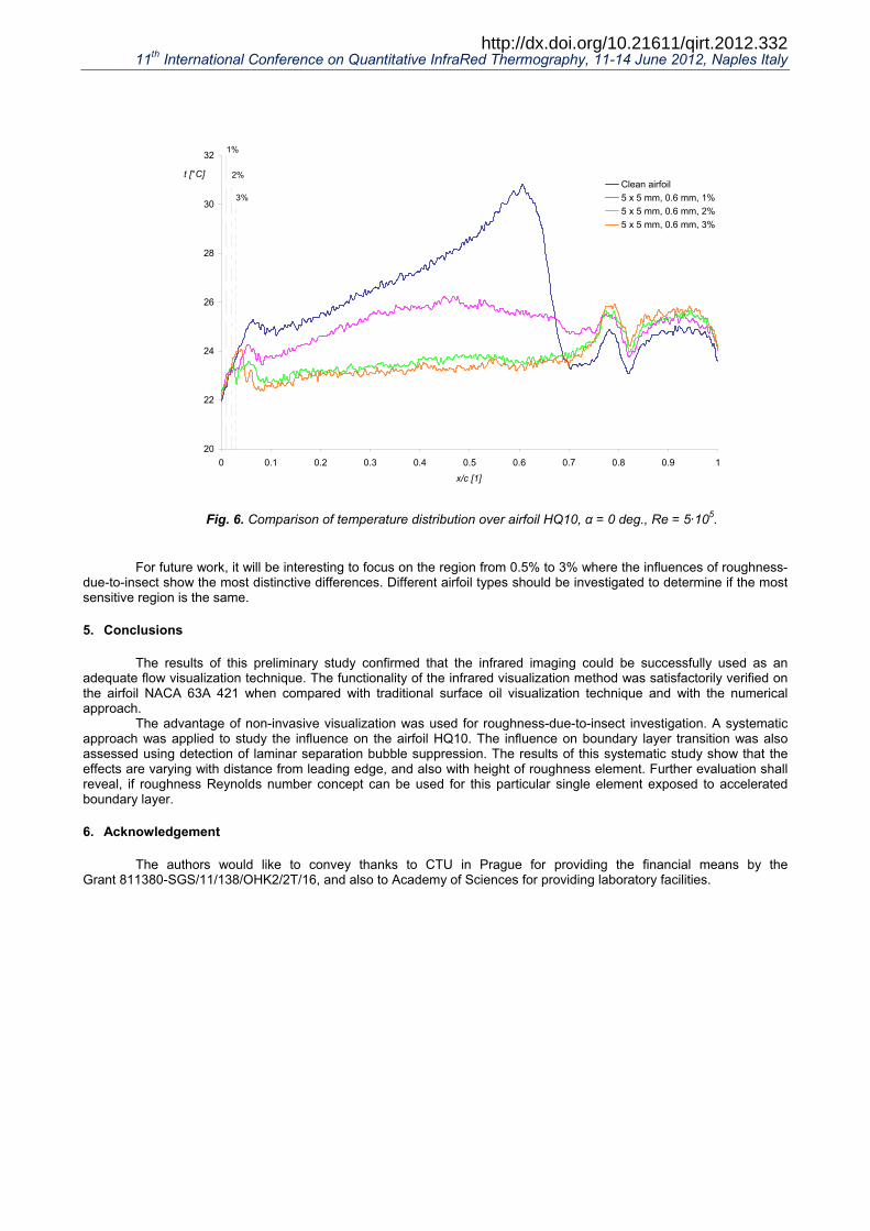
The results from the second case are shown in figure 5. For each element the temperature profile over the airfoil passing through the axis of the element was also plotted. Then, the clean airfoil temperature profile was added. All the plotted profiles were normalized to the chord of airfoil for the comparison of the results. It was demonstrated that all elements significantly affected the boundary layer – suppressed the laminar separation bubble by speeding up the transition to turbulence.

Fig. 5. Comparison of single roughness element located at 1%, 3%, 5% x/c (from top to bottom), size 5 x 5 mm, height 0.6 mm, α = 0 deg., Re = 5·105, airfoil HQ10.

31°C

21°C

31°C 21°C



20

22

24

26

28

30

32

0 0.1 0.2 0.3 0.4 0.5 0.6 0.7 0.8 0.9 1

x/c [1]

t [°C]Clean airfoil5 x 5 mm, 0.6 mm, 1%5 x 5 mm, 0.6 mm, 2%5 x 5 mm, 0.6 mm, 3%

1% 2% 3%

Fig. 6. Comparison of temperature distribution over airfoil HQ10, α = 0 deg., Re = 5·105.

For future work, it will be interesting to focus on the region from 0.5% to 3% where the influences of roughness-

due-to-insect show the most distinctive differences. Different airfoil types should be investigated to determine if the most sensitive region is the same.

5. Conclusions

The results of this preliminary study confirmed that the infrared imaging could be successfully used as an adequate flow visualization technique. The functionality of the infrared visualization method was satisfactorily verified on the airfoil NACA 63A 421 when compared with traditional surface oil visualization technique and with the numerical approach.

The advantage of non-invasive visualization was used for roughness-due-to-insect investigation. A systematic approach was applied to study the influence on the airfoil HQ10. The influence on boundary layer transition was also assessed using detection of laminar separation bubble suppression. The results of this systematic study show that the effects are varying with distance from leading edge, and also with height of roughness element. Further evaluation shall reveal, if roughness Reynolds number concept can be used for this particular single element exposed to accelerated boundary layer.

6. Acknowledgement

The authors would like to convey thanks to CTU in Prague for providing the financial means by the Grant 811380-SGS/11/138/OHK2/2T/16, and also to Academy of Sciences for providing laboratory facilities.



Nomenclature (units added)

A heat transfer area of the surface, m2 C1 first radiant constant, W·m2

C2 second radiant constant, m·K

Hλ spectral radiant emittance, W·m-3

Me total emittance, W·m-2 Re Reynolds number, 1 T thermodynamic temperature, K ΔT temperature gradient (difference between the surface and the fluid temperature), K Tu turbulence intensity, % cf,x local skin friction coefficient, 1 h convective heat transfer coefficient, W·m-2·K-1 hx local convective heat transfer coefficient, W·m-2·K-1 q heat transferred per unit time, W t temperature, °C wx local flow velocity, m·s-1 x absolute distance from leading edge, m x/c distance from leading edge related to airfoil chord, 1 α angle of attack, deg. δ boundary layer thickness, m ε emissivity, 1 ελ spectral emissivity, 1 λ wavelength, m λc heat conductivity of fluid, W·m-1·K-1 ν kinematic viscosity of fluid, m2·s-1 σ Stephan-Boltzmann constant, W·m-2·K-4

REFERENCES

[1] Quast A. W., “Detection of transition by infrared image technique”. Proceedings of XX OSTIV Congress, Benalla, Australia, 1987.

[2] de Luca L., Carlomagno G. M., Buresti G., Toutain J., "Boundary layer diagnostics by means of an infrared scanning radiometer". Experiments in Fluids, vol. 9, no. 3, pp. 121-128, 1990.

[3] Kuklova J., “Metody vizualizace proudeni na obtekanem telese”. Bachelor thesis, CTU in Prague, Prague, 2010. [4] Popelka L., Kuklova J., Simurda D., Souckova N., Matejka M., Uruba V., “Visualization of boundary layer

separation and passive flow control on airfoils and bodies in wind-tunnel and in-flight experiments”. Proceedings of EFM12 – Experimental Fluid Mechanics 2012, Jicin, Czech Republic, 2012.

[5] Souckova N., Kuklova J., Popelka L., Matejka M., “Visualization of flow separation and control by vortex generators on an single flap in landing configuration”. Proceedings of EFM11 – Experimental Fluid Mechanics 2011, Liberec, Czech Republic, 2011.

[6] Drela M., Youngren H., “Xfoil 6.9”. User Guide. MIT, 2001, http://web.mit.edu/drela/Public/web/xfoil/xfoil_doc.txt.



Documents

Visualization of Airfoil Boundary Layer by Infrared - QIRT