Visualization and Confirmatory Clustering of Sequence Data from a Simulation-Based Assessment Task

Yoav Bergner, Zhan Shu, and Alina A. von Davier Educational Testing Service

Princeton, NJ 08541 {ybergner,zshu,avondavier}@ets.org

ABSTRACTChallenges of visualization and clustering are explored with respect to sequence data from a simulation-based assessment task. Visualization issues include representing progress towards a goal and accounting for variable-length sequences. Clustering issues focus on external criteria with respect to official scoring rubrics of the same sequence data. The analysis has a confirmatory flavor; the goal is to understand to what extent clustering solutions align with score categories. It is found that choices related to data preprocessing, distance metric and external cluster validity measures all impact agreement between cluster assignments and scores. This work raises key issues about clustering of educational data, especially in the presence of multidimensionality. Different clustering protocols may lead to different solutions, no one of which is uniquely best.

KeywordsSequence mining, clustering, visualization, simulation-based tasks, assessment

1. INTRODUCTIONComplex tasks in educational environments are intended to be more engaging for learners and more reflective of real life challenges than traditional test items [22]. In an assessment context at least, the additional time it takes to administer such tasks comes at a certain cost. One hopes therefore that data relating to the process provide more information than the outcome of the task alone. Examples of such process data range in complexity: they may include simple measures like response time [21], multiple attempt records [2], and use of hints [20]; or more expansive processes such as referencing a range of online learning resources [37], keystroke-level writing data [1], or actions taken in a simulation- or game-based task [18, 25]. One broad characterization of the data at the latter end of this list is that they comprise sequences of observable states. Temporal information about the duration of each state may be included or not.

Clustering sequences is a way to detect similar patterns of behavior. In an educational context, the hope is that this structure is informative of some underlying characteristic, perhaps style, perhaps ability. From the perspective of learning scientists and instructional designers, it is important to understand both of these aspects, and from an assessment perspective, it is important to

distinguish between them. In other words, patterns in the structure of responses may detect both construct-relevant and construct-irrelevant variance, and the distinction is critical for validity in the interpretation of scores [16]. We consider sequence data from a particular simulation based task, the Wells task used by the National Assessment for Educational Progress (NAEP) as part of the Technology and Engineering Literacy (TEL) Assessment [26]. The sequence data from Wells are only modestly complex as sequence data go, but their analysis introduces a number of operational choices. To map out the challenges to the data analyst, we organize some of these loosely into challenges of visualizing sequence data (and associated frequency or summary data) and challenges of clustering the sequences.

The Wells task is scored along two cognitive dimensions by separate rubrics. Our goal is not to reproduce the results of the rubrics after the fact by alternate means. Instead we ask whether a bottom-up search for patterns in the data comes close to approximating the top-down scoring design in the scores of the sequences, and if not, why not? The analysis thus has a confirmatory flavor. We fully expect the two approaches not to meet in the middle, but hope that there may be insights to gain about principles of scoring and/or clustering from the concordance of scores with cluster assignments.

The organization of the paper is as follows: in section 2 we describe related work on clustering and sequence mining. In section 3, we describe the NAEP task, scoring design, and the sequence data. Section 4 introduces two operational choices that affect the visualization of the data, while section 5 addresses choices with respect to clustering. Section 6, describes resulting measures of external validity when comparing cluster assignments to score categories. Section 7 includes a discussion of the results with extensions to future work.

2. RELATED WORKClustering student actions is a common approach to various types of educational data. Some recent applications include reading comprehension tasks [28], discussion forum behavior [4, 23], collaborative learning sessions [29], automated speech act detection [33], and strategies in educational games [18, 25]. Most clustering studies operate on feature vectors from logs, not on sequences of states themselves. This is an important distinction. Whether feature vectors are numerical in nature (counts, ratios, etc.) or coded as binary indicators (e.g. [18]), such vectors are all the same length and permit straightforward metrics such as Manhattan, Euclidean, or cosine distance functions. Though their clustering analysis used only feature vectors, exploratory sequential pattern mining also figured in [29]. Time-series data and an agglomerative approach similar to ours was used in [4], but with a key difference. That analysis mapped each possible action type (e.g., reading or writing) to its own binary-valued time-series

Proceedings of the 7th International Conference on Educational Data Mining (EDM 2014) 177

using an indicator, and only clustered students based on one type of action at a time. Such binary data types do not invoke the same sequence matching issues.

Many of the issues encountered here arose in the context of clustering web sessions from online learning environments in [37], namely: the desire to mine categorical activity sequences, rather than sets or counts of actions; the need to introduce appropriate similarity measures on these sequences; and lastly, the challenges of cluster validation. This work introduced several new algorithms and reported on the performance and scaling of these, but did not say much about cluster interpretation issues. Our approach and toolset is similar to those used by [7] to explore study patterns and identify groups, although there again the analysis was exploratory.

In fact, most if not all of the studies mentioned above used clustering either in an exploratory fashion, or to examine correlation, for example with levels of answers to reading questions [28] or to course pass-fail rates [23]. In our application, by contrast, the student sequences are actually scored by an operational rubric (along two dimensions, as will be discussed). By looking closely at the external validity of our clustering results with respect to rubric-based scores, our analysis has a more confirmatory flavor. This paper thus contributes both a new application of sequence clustering methods in an assessment context and an extension of the discussion on cluster validity with respect to expert-based measures.

The first part of this paper also concerns ordering a set of actions in a sequence with regard to proximity to the end-goal. Sequences of actions are not always goal oriented, for example when they describe web sessions or studying behaviors. Even in the cases where the activity itself has a goal, it is not always straightforward to tell whether the user activity represents movement towards or away from the goal, especially when the state space is large. Estimating the probabilistic distance to solution in computer programming exercises was the subject of [36]. Networks of states and actions in a logic tutor were analyzed using a novel data structure in [8], and social network methods were used to identify both solution sub-goals and conceptual problem areas. In our application, this task is much easier because the state space is small. However, one can imagine generalizations of the task or other simulation-based task applications, in which these probabilistic methods would be quite useful.

Finally, alternatives to clustering in analysis of sequential data include approaches such as differential sequence mining [24] or the use of hidden or dynamic Markov models [19, 35] to distinguish successful sequences from unsuccessful sequences. Complex feature engineering, as in the design of affect detectors [3, 6], can also account for many of the salient features of sequential data. All of these approaches may be more applicable to open-ended group or individual problem solving sessions than to a task such as ours where success depends deterministically on certain actions and all of the sequences are ultimately successful.

3. DATA FROM THE WELLS TASKThe data for our analysis (sample size N=1318) come from a pilot administration of TEL tasks by NAEP in 2013. The Wells task has been publicly released on the NAEP website [27].

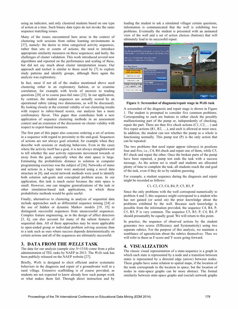
Briefly, Wells is designed to elicit efficient and/or systematic behaviors in the diagnosis and repair of a groundwater well in a rural village. Extensive scaffolding is of course provided, as students are not expected to know already how such pumps work or what makes them fail. Through direct instruction and by

leading the student to ask a simulated villager certain questions, information is communicated that the well is exhibiting two problems. Eventually the student is presented with an animated view of the well and a set of action choices (buttons) that will ultimately lead to its successful repair.

Copyright © 2013 by Educational Testing Service. All rights reserved.Copyright © 2013 by Educational Testing Service. All rights reserved.

Wells, an NAEP Example

Figure 1: Screenshot of diagnosis/repair stage in Wells task A screenshot of the diagnosis and repair stage is shown in Figure 1. The student is prompted to consider five common problems.Corresponding to each are buttons to either check the possibly malfunctioning part of the pump or, independently of checking, repair the part. There are thus five check actions (C1, C2, …) and five repair actions (R1, R2, …), and each is allowed at most once. In addition, the student can test whether the pump as a whole is functioning normally. This pump test (P) is the only action that can be repeated.

The two problems that need repair appear (always) in positions four and five, i.e., C4, R4 check and repair one of them, while C5, R5 check and repair the other. Once the broken parts of the pump have been repaired, a pump test ends the task with a success message. As the action set is small and students are allocated plenty of time to complete the task, all students reach the end goal of the task, even if they do so by random guessing.

For example, a student sequence during the diagnosis and repair might be recorded as follows:

C1, C2, C3, C4, R4, P, C5, R5, P

Since the only problems with the well correspond numerically to problem 4 and 5, this sequence might correspond to a student who has not gained (or acted on) the prior knowledge about the problems exhibited by the well. Because such knowledge is possible from the information provided, the sequence C4, R4, P, C5, R5, P is very common. The sequence C5, R5, P, C4, R4, P should presumably be equally good. We will return to this point. In practice, the sequence of observed actions by the student generates two scores (Efficiency and Systematicity) using two separate rubrics. For the purpose of this analysis, we maintain a semblance of agnosticism about the rubrics themselves. Thus we will refer to these as F-score and Y-score going forward.

4. VISUALIZATIONThe classic visual representation of a state-sequence is a graph in which each state is represented by a node and a transition between states is represented by a directed edge (arrow) between nodes. These graphs have some relation to spatial maps, if the location of the node corresponds to the location in space, but the location of nodes in state-space graphs can be more abstract. The formal similarity between state-space graphs and (social) network graphs

Proceedings of the 7th International Conference on Educational Data Mining (EDM 2014) 178

has invited more than one application of methods of network analysis to sequence mining [8, 34].

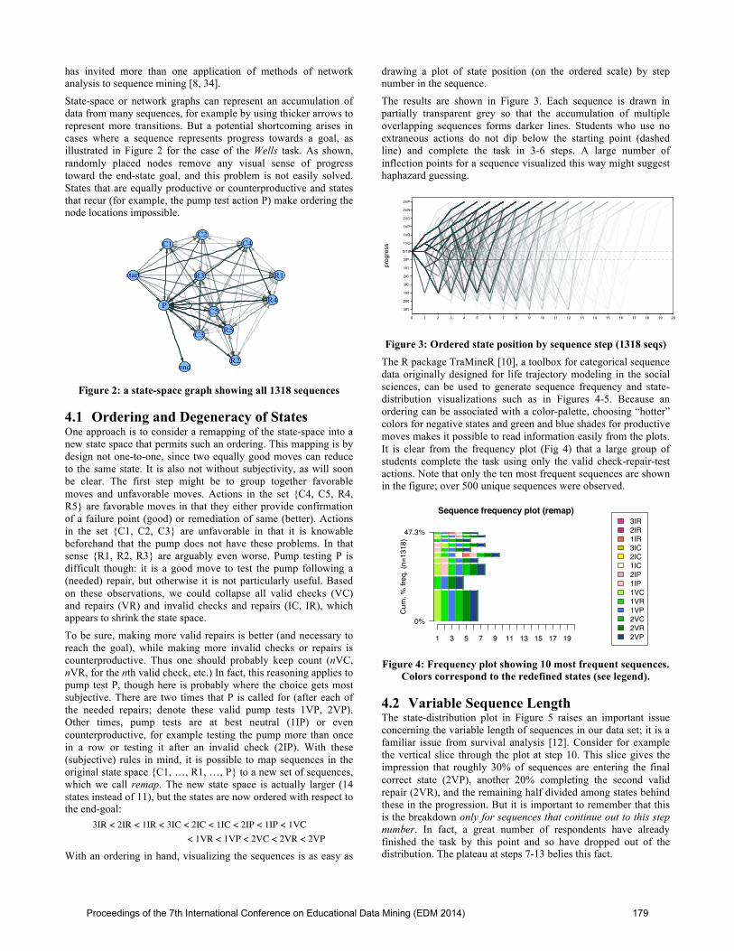
State-space or network graphs can represent an accumulation of data from many sequences, for example by using thicker arrows to represent more transitions. But a potential shortcoming arises in cases where a sequence represents progress towards a goal, as illustrated in Figure 2 for the case of the Wells task. As shown, randomly placed nodes remove any visual sense of progress toward the end-state goal, and this problem is not easily solved. States that are equally productive or counterproductive and states that recur (for example, the pump test action P) make ordering the node locations impossible.

start

C1C2

C3

C4

C5

R1

R2

R3

R4

R5

P

end

Figure 2: a state-space graph showing all 1318 sequences

4.1 Ordering and Degeneracy of States One approach is to consider a remapping of the state-space into a new state space that permits such an ordering. This mapping is by design not one-to-one, since two equally good moves can reduce to the same state. It is also not without subjectivity, as will soon be clear. The first step might be to group together favorable moves and unfavorable moves. Actions in the set {C4, C5, R4, R5} are favorable moves in that they either provide confirmation of a failure point (good) or remediation of same (better). Actions in the set {C1, C2, C3} are unfavorable in that it is knowable beforehand that the pump does not have these problems. In that sense {R1, R2, R3} are arguably even worse. Pump testing P is difficult though: it is a good move to test the pump following a (needed) repair, but otherwise it is not particularly useful. Based on these observations, we could collapse all valid checks (VC) and repairs (VR) and invalid checks and repairs (IC, IR), which appears to shrink the state space.

To be sure, making more valid repairs is better (and necessary to reach the goal), while making more invalid checks or repairs is counterproductive. Thus one should probably keep count (nVC, nVR, for the nth valid check, etc.) In fact, this reasoning applies to pump test P, though here is probably where the choice gets most subjective. There are two times that P is called for (after each of the needed repairs; denote these valid pump tests 1VP, 2VP). Other times, pump tests are at best neutral (1IP) or even counterproductive, for example testing the pump more than once in a row or testing it after an invalid check (2IP). With these (subjective) rules in mind, it is possible to map sequences in the original state space {C1, …, R1, …, P} to a new set of sequences, which we call remap. The new state space is actually larger (14 states instead of 11), but the states are now ordered with respect to the end-goal:

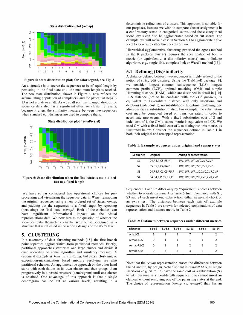
3IR < 2IR < 1IR < 3IC < 2IC < 1IC < 2IP < 1IP < 1VC < 1VR < 1VP < 2VC < 2VR < 2VP

With an ordering in hand, visualizing the sequences is as easy as

drawing a plot of state position (on the ordered scale) by step number in the sequence.

The results are shown in Figure 3. Each sequence is drawn in partially transparent grey so that the accumulation of multiple overlapping sequences forms darker lines. Students who use no extraneous actions do not dip below the starting point (dashed line) and complete the task in 3-6 steps. A large number of inflection points for a sequence visualized this way might suggest haphazard guessing.

time

progress

3IR

2IR

1IR

3IC

2IC

1IC

2IP

0/1IP

1VC

1VR

1VP

2VC

2VR

2VP

0 1 2 3 4 5 6 7 8 9 10 11 12 13 14 15 16 17 18 19 20

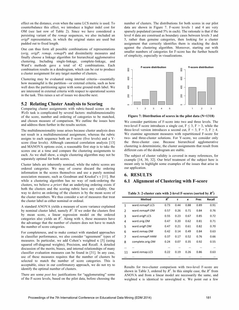
Figure 3: Ordered state position by sequence step (1318 seqs) The R package TraMineR [10], a toolbox for categorical sequence data originally designed for life trajectory modeling in the social sciences, can be used to generate sequence frequency and state-distribution visualizations such as in Figures 4-5. Because an ordering can be associated with a color-palette, choosing “hotter” colors for negative states and green and blue shades for productive moves makes it possible to read information easily from the plots. It is clear from the frequency plot (Fig 4) that a large group of students complete the task using only the valid check-repair-test actions. Note that only the ten most frequent sequences are shown in the figure; over 500 unique sequences were observed.

Sequence frequency plot (remap)

Cum

. % fr

eq. (

n=13

18)

1 3 5 7 9 11 13 15 17 19

0%

47.3%3IR2IR1IR3IC2IC1IC2IP1IP1VC1VR1VP2VC2VR2VP

Figure 4: Frequency plot showing 10 most frequent sequences. Colors correspond to the redefined states (see legend).

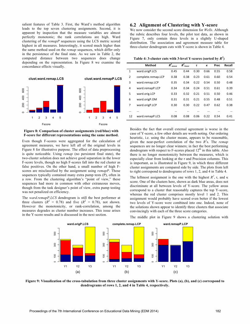
4.2 Variable Sequence Length The state-distribution plot in Figure 5 raises an important issue concerning the variable length of sequences in our data set; it is a familiar issue from survival analysis [12]. Consider for example the vertical slice through the plot at step 10. This slice gives the impression that roughly 30% of sequences are entering the final correct state (2VP), another 20% completing the second valid repair (2VR), and the remaining half divided among states behind these in the progression. But it is important to remember that this is the breakdown only for sequences that continue out to this step number. In fact, a great number of respondents have already finished the task by this point and so have dropped out of the distribution. The plateau at steps 7-13 belies this fact.

Proceedings of the 7th International Conference on Educational Data Mining (EDM 2014) 179

State distribution plot (remap)Fr

eq. (

n=13

18)

1 3 5 7 9 11 13 15 17 19

0.0

0.2

0.4

0.6

0.8

1.0

Figure 5: state distribution plot; for color legend, see Fig. 3

An alternative is to coerce the sequences to be of equal length by persisting in the final state until the maximum length is reached. The new state distribution, shown in Figure 6, now reflects the accumulating population of completers, and the plateau at steps 7-13 is not a plateau at all. As we shall see, this manipulation of the sequence data also has a significant effect on clustering results, because it alters the similarity measure between two sequences when standard edit distances are used to compare them.

State distribution plot (remaPersist)

Freq

. (n=

1318

)

T1 T3 T5 T7 T9 T11 T13 T15 T17 T19

0.0

0.2

0.4

0.6

0.8

1.0

Figure 6: State distribution when the final state is maintained out to a fixed length

We have so far considered two operational choices for pre-processing and visualizing the sequence data in Wells: remapping the original sequences using a new ordered set of states, remap, and padding out the sequences to a fixed length by repeating (persisting) the final state, remapP. Both of these choices can have significant informational impact on the visual representations data. We now turn to the question of whether the sequence data themselves can be seen to self-organize in a structure that is reflected in the scoring designs of the Wells task.

5. CLUSTERINGIn a taxonomy of data clustering methods [15], the first branch point separates agglomerative from partitional methods. Briefly, partitional approaches start with one large cluster and divide it once according to some algorithm and similarity measure. A canonical example is k-means clustering, but fuzzy clustering or expectation-maximization based mixture resolving are also partitional schemes. An agglomerative approach on the other hand starts with each datum as its own cluster and then groups them progressively in a nested structure (dendrogram) until one cluster is obtained. One advantage of this approach is that a single dendrogram can be cut at various levels, resulting in a

deterministic refinement of clusters. This approach is suitable for our purposes, because we wish to compare cluster assignments in a confirmatory sense to categorical scores, and these categorical score levels can also be agglomerated based on cut scores. For example, we will make a case in Section 6.1 to agglomerate a five level F-score into either three levels or two. Hierarchical agglomerative clustering (we used the agnes method in the R package cluster) requires the specification of both a metric (or equivalently, a dissimilarity matrix) and a linkage algorithm, e.g., single-link, complete-link or Ward’s method [15].

5.1 Defining (Dis)similarity A distance defined between two sequences is highly related to the notion of string edit distance. Using the TraMineR package [9], we consider longest common subsequence (LCS), longest common prefix (LCP), optimal matching (OM) and simple Hamming distance (HAM), which are described in detail in [10]. LCS distance (not to be confused with the LCS problem) is equivalent to Levenshtein distance with only insertions and deletions (indel cost 1), no substitutions. In optimal matching, one also specifies a substitution matrix. For example, the substitution cost may be computed based on transition rates, in order to accentuate rare events. With a fixed substitution cost of 2 and indel cost of 1, the OM distance metric is equivalent to LCS. We used OM with a fixed indel cost of 3 to distinguish this metric, as illustrated below. Consider the sequences defined in Table 1 in both their original and remapped representation:

Table 1: Example sequences under original and remap states  

Sequences S1 and S2 differ only by “equivalent” choices between whether to operate on issue 4 or issue 5 first. Compared with S1, S3 and S4 each insert one extra action, either an invalid check or an extra test. The distances between each pair of example sequences in Table 1 are shown for selected combinations of data representation and distance metric in Table 2.

Table 2: Distances between sequences under different metrics

Note that the remap representation erases the difference between the S1 and S2, by design. Note also that in remapP.LCS, all single insertions (e.g. S1 to S3) have the same cost as a substitution (S3 to S4), because in a fixed-length sequence, one cannot insert an element without removing one of the persisting states at the end. The choice of representation (remap vs. remapP) thus has an

Sequence   Original   remap  representation  

S1   C4,R4,P,C5,R5,P   1VC,1VR,1VP,2VC,2VR,2VP  

S2   C5,R5,P,C4,R4,P   1VC,1VR,1VP,2VC,2VR,2VP  

S3   C4,R4,P,C1,C5,R5,P   1VC,1VR,1VP,1IC,2VC,2VR,2VP  

S4   C4,R4,P,P,C5,R5,P   1VC,1VR,1VP,2IP,2VC,2VR,2VP  

Distance   S1-­‐S2   S1-­‐S3   S1-­‐S4   S2-­‐S3   S2-­‐S4   S3-­‐S4  

orig.LCS   6   1   1   7   7   2  

remap.LCS   0   1   1   1   1   2  

remapP.LCS   0   2   2   2   2   2  

remap.OM   0   3   3   3   3   2  

Proceedings of the 7th International Conference on Educational Data Mining (EDM 2014) 180

effect on the distance, even when the same LCS metric is used. To counterbalance this effect, we introduce a higher indel cost for OM (see last row of Table 2). Since we have considered a persisting variant of the remap sequences, we also included an origP representation, in which the original states are used but padded out to fixed length. One can thus form all possible combinations of representations (orig, origP, remap, remapP) and dissimilarity measures and finally choose a linkage algorithm for hierarchical agglomerative clustering. Including single-linkage, complete-linkage, and Ward’s methods gave a total of 42 combinations. Each combination results in a dendrogram, which can be cut to produce a cluster assignment for any target number of clusters.

Clustering may be evaluated using internal criteria—essentially how meaningful is the partition—or external criteria, such as how well does the partitioning agree with some ground-truth label. We are interested in external criteria with respect to operational scores in the task. This raises a set of issues we describe next.

5.2 Relating Cluster Analysis to Scoring Comparing cluster assignments with rubric-based scores on the Wells task is complicated by several factors: multidimensionality of the score, number and ordering of categories to be matched, and chosen measure of comparison. We outline the issues here and address them further in the results section.

The multidimensionality issue arises because cluster analysis does not result in a multidimensional assignment, whereas the rubric assigns to each sequence both an F-score (five levels) and a Y-score (four levels). Although canonical correlation analysis [13] and MANOVA options exist, a reasonable first step is to take the scores one at a time and compare the clustering assignments to each. As we shall show, a single clustering algorithm may not be separately optimal for both scores.

Cluster labels are inherently nominal, while the rubric scores are ordered categories. We may of course discard the ordering information in the scores themselves and use a purely nominal association measure, such as Goodman and Kruskal’s τ [11]. But while a clustering algorithm has no way of rank-ordering the clusters, we believe a priori that an underlying ordering exists if both the clusters and the scoring rubric have any validity. One way to derive an ordering of the clusters is by the mean score of the cluster members. We thus consider a set of measures that treat the cluster label as either nominal or ordinal. A standard ANOVA yields a measure of score variance explained by nominal cluster label, namely R2. If we order the clusters first by mean score, a linear regression model on the ordered categories also yields an R2. Along with τ, these measures have the advantage that the number of clusters does not have to match the number of score categories.

For completeness, and to make contact with standard approaches in classifier performance, we also consider “agreement” types of measures. In particular, we add Cohen’s weighted κ [5] (using squared off-diagonal weights), Precision, and Recall. A detailed discussion of the merits, biases, and internal relationships of many classifier evaluation measures can be found in [31]. In any case, use of these measures requires that the number of clusters be selected to match the number of score categories. This is acceptable, since in our confirmatory approach, we do not try to identify the optimal number of clusters.

There are some post hoc justifications for “agglomerating” some of the F-score levels, based on the pilot data, before choosing the

number of clusters. The distributions for both scores in our pilot data are shown in Figure 7. F-score levels 1 and 4 are very sparsely populated (around 5% in each). The rationale is that if the level 4 data are construed as boundary cases between levels 3 and 5, rather than genuine categories, then looking for a cluster assignment that correctly identifies them is stacking the deck against the clustering algorithm. Moreover, starting out with smaller numbers of categories for F-score has the further benefit of simplicity, especially in visualizations.

1 2 3 4 5

F-score distribution

0200

400

600

800

1 2 3

Y-score distribution

0200

400

600

800

Figure 7: Distribution of scores in the pilot data (N=1318) We consider partitions of F-score into two and three levels. The two-level F-score introduces a single cut, F ≤ 3, F > 3, while the three-level version introduces a second cut, F < 3, F = 3, F ≥ 4. We examine agreement measures with repartitioned F-score for two- and three-cluster solutions. For Y-score, we consider only the three-cluster case. Because hierarchical agglomerative clustering is deterministic, the cluster assignments that result from different cuts of the dendrogram are stable. The subject of cluster validity is covered in many references, for example [14, 30, 32]. Our brief treatment of the subject here is meant only to highlight some examples of the issues that arise in our application.

6. RESULTS6.1 Alignment of Clustering with F-score

Table 3: 2-cluster cuts with 2-level F-scores (sorted by R2)

Method   R2   τ   κ   Prec   Recall  

1   ward.remapP.LCS   0.73   0.44   0.88   0.89   0.91  

2   ward.remapP.OM   0.57   0.26   0.71   0.84   0.76  

3   ward.origP.LCS   0.55   0.23   0.67   0.85   0.72  

4   ward.orig.OM   0.47   0.20   0.62   0.81   0.71  

5   ward.origP.OM   0.47   0.21   0.61   0.82   0.70  

6   ward.remap.OM   0.42   0.14   0.49   0.84   0.63  

7   ward.remapP.HAM   0.37   0.17   0.52   0.76   0.66  

8   complete.orig.OM   0.24   0.07   0.35   0.92   0.55  

…   …   …   …   …   …   …  

11   ward.remap.LCS   0.22   0.19   0.26   0.86   0.63  …   …   …   …   …   …   …  

Results for two-cluster comparison with two-level F-score are shown in Table 3, ordered by R2. In this simple case, the R2 from ANOVA and from a linear model are necessarily the same, and weighted κ is identical to unweighted κ. We point out a few

Proceedings of the 7th International Conference on Educational Data Mining (EDM 2014) 181

salient features of Table 3. First, the Ward’s method algorithm leads to the top seven clustering assignments. Second, it is apparent by inspection that the measure variables are almost perfectly monotonic; the rank correlations are high. Ward clustering of the remapP sequences using the LCS metric scored highest in all measures. Interestingly, it scored much higher than the same method used on the remap sequences, which differ only in the persistence of the final state. As we saw in Table 2, the computed distance between two sequences does change depending on the representation. In Figure 8 we examine the concordance effects visually.

1 2 3 4 5

clust.ward.remap.LCS

Fscore

0200

400

600

1 2 3 4 5

clust.ward.remapP.LCS

Fscore

0200

400

600

Figure 8: Comparison of cluster assignments (red/blue) with F-score for different representations using the same method.

Even though F-scores were aggregated for the calculation of agreement measures, we have left all of the original levels in Figure 8 for illustrative purpose. The effect of data preprocessing is quite noticeable. Using remap (no persistent final state), the two-cluster solution does not achieve good separation in the lower F-score levels, though no high F-scores fall into the red cluster as false positives. On the other hand, a small number of high F-scores are misclassified by the assignment using remapP. Those sequences typically contained many extra pump tests (P), often in a row. From the clustering algorithm’s “point of view,” these sequences had more in common with other extraneous moves, though from the task designer’s point of view, extra pump testing was not penalized on efficiency. The ward.remapP.LCS dendrogram is still the best performer at three clusters (R2 = 0.78) and five (R2 = 0.78), not shown. However the monotonicity, or rank-correlation, among the measures degrades as cluster number increases. This issue arises in the Y-score results and is discussed in the next section.

6.2 Alignment of Clustering with Y-score We now consider the second score dimension for Wells. Although the rubric describes four levels, the pilot test data, as shown in Figure 7, only contain three levels in a slightly U-shaped distribution. The association and agreement measure table for three-cluster dendrogram cuts with Y-score is shown in Table 4.

Table 4: 3-cluster cuts with 3-level Y-scores (sorted by R2)

Besides the fact that overall external agreement is worse in the case of Y-score, a few other details are worth noting. Our ordering heuristic, i.e. using the cluster means, appears to be reasonable, given the near-perfect correlation of the two R2s. The remap sequences are no longer clear winners; in fact the best performing dendrogram with respect to F-scores placed 12th in this table. Also there is no longer monotonicity between the measures, which is especially clear from looking at the τ and Precision columns. This is important, as is illustrated in Figure 9, in which three different cluster assignments are compared side by side. The plots from left to right correspond to dendrograms of rows 1, 2, and 4 in Table 4. The leftmost assignment is the one with the highest R2, τ, and κ score. One of the clusters here, shown as dark blue areas, does not discriminate at all between levels of Y-score. The yellow areas correspond to a cluster that reasonably captures the top Y-score, whereas the red cluster comprises mostly level 1 and 2. This assignment would probably have scored even better if the lowest two levels of Y-score were combined into one. Indeed, none of the solutions shown appear to identify three clusters that associate convincingly with each of the three score categories.

The middle plot in Figure 9 shows a clustering solution with

Method   R2anova   R2

linear   τ   κ   Prec   Recall  

1   ward.origP.LCS   0.45   0.44   0.30   0.66   0.55   0.58  

2   complete.remap.LCP   0.38   0.38   0.23   0.61   0.60   0.54  

3   ward.remap.LCP   0.35   0.34   0.22   0.54   0.50   0.48  

4   ward.remapP.LCP   0.34   0.34   0.24   0.51   0.61   0.39  

5   ward.orig.LCP   0.33   0.32   0.21   0.51   0.50   0.46  

6   ward.origP.OM   0.31   0.31   0.21   0.55   0.48   0.51  

7   ward.origP.LCP   0.30   0.30   0.22   0.47   0.62   0.38  

…   …   …   …   …   …   …   …  

12   ward.remapP.LCS   0.08   0.08   0.06   0.22   0.54   0.41  

ward.origP.LCS

(a)

0100

300

500

Y1 Y2 Y3

(a)

complete.remap.LCP

0100

300

500

Y1 Y2 Y3

(b)

ward.remapP.LCP

0100

300

500

Y1 Y2 Y3

(c)

Figure 9: Visualization of the cross-tabulation from three cluster assignments with Y-score. Plots (a), (b), and (c) correspond to dendrograms of rows 1, 2, and 4 in Table 4, respectively.

Proceedings of the 7th International Conference on Educational Data Mining (EDM 2014) 182

lower R2, τ, and κ, but a higher Precision. It also has a non-discriminating cluster, though here it is smaller. The yellow and red clusters are more or less equally split on the mid-level score.

Finally the rightmost clustering has slightly higher precision, but low recall, R2 and κ. According to τ, it is the second best match to the scores. One is tempted to say that this cluster assignment “avoids getting it wrong.” Although many more sequences are put into the non-discriminating blue cluster, including all of the mid-level Y-score, the red and yellow clusters have no false positives at all. Depending on the purpose, for example routing in a multi-stage assessment [38], it might be argued that this “diagnostic” clustering is preferable.

After varying the data representation, distance metric and even linkage function, examining alignment of clustering solutions with Y-score turns out to be rather subtle.

6.3 Alignment of Clustering with Both Scores The best cluster dendrogram for F-score is a poor performer with respect to Y-scores (and vice-versa). Using MANOVA with both scores simultaneously, ward.remapP.LCS is still the winner (likewise if a combined six-level FY-score—two F-score levels and three Y-score levels—is matched to a six-cluster cut). It wins despite not resolving the Y-scores well, just on account of resolving the F-score as well as it does. The logical conclusion to draw from this is that, in the case of multidimensional scores, there is no one best clustering assignment. The appropriate clustering method and preprocessing of the data indeed depend on the intended purpose.

7. DISCUSSION AND FUTURE WORKWe have tried to show some of the operational issues that arise in characterizing sequence data from a simulation-based task, specifically visualization and clustering choices. With respect to visualization, we were concerned with representing progress as unambiguously as possible, and we explored the consequences of both mapping the original sequences to an ordered set of states and padding out the sequences to a fixed length.

With respect to clustering, we were most interested in measures of external agreement with the two-dimensional scoring rubric designed for the task. We found that the clustering dendogram that worked best in terms of one score did not necessarily work at all in terms of the other. Both data preprocessing and selection of the between-sequence distance metric had an impact, though the best agglomerative linkage algorithm was almost always Ward’s method. In the case of Y-score, while none of the solutions were great, we found it ambiguous to tell which was even the best among the mediocre. Whether this reflects a feature of the Y-scoring that is ambiguous or just difficult to capture via sequence clustering is something we wish to investigate further.

This work raises important issues about clustering of educational sequence data in the presence of multidimensionality: two different clustering protocols may reach different solutions, both of them valid. Furthermore, brute force search among clustering solutions for a best fit according to one particular external criterion may exclude solutions of interest. In practice, what this of course suggests is that the use of sequence clustering methods for inference needs to be handled with care.

Without a doubt, much prior knowledge goes in to preprocessing educational data already. For example, we often simply exclude events we are not interested in. In the context of sequential data, an alternative might be to assign selective weights to particular insertions, deletions and substitutions of states. The web-page

similarity index in [37] is designed to address this issue, because substituting one web page with a very different one should be treated distinctly from substituting similar pages. In our case, for example, a variable insertion cost for pump test actions P would have affected the agreement of cluster assignment with F-score.

F-score and Y-score indeed stand for real constructs in the rubric design: efficiency and systematicity. We found that grouping by efficiency can be discovered through sequence clustering, but systematicity was not as well matched. If sequences with the same score do not self-group under edit distance, these discrepancies may merit closer examination. This is the confirmatory value of performing such an analysis.

The edit-distance similarity measures that we used here do not embed sequence data in a multidimensional coordinate space, whereas feature-vector descriptions of sequences do. The latter approach might have several advantages when the external measure is also multidimensional, as in the case of our expert-based scores. Methods like canonical analysis [13] may be brought to bear on such multivariate data. Standard distance metrics also make internal cluster quality analysis more straightforward. While we did not delve here into such measures, it turns out that many internal cluster criteria are not well suited to the use of generalized dissimilarity, for example because a cluster “centroid” is not easily defined. Some authors have cautioned against using Ward’s method with non-Euclidean distances because of interpretability problems [17], although this prohibition would have removed the best clustering solutions—by external criteria—in our study. The lack of appropriate internal indices is an unsolved problem that we plan to investigate further.

We note that ordering effects in the data were likely introduced by the fixed order of presentation in the task itself. The five sets of buttons corresponding to possible problems with the well were presented vertically and always in the order corresponding to the codes numbered 1-5. Within the sequence data, the two valid checks, C4 and C5, occurred in that order nine times as often as the reverse, and unnecessary check C2 preceded C3 almost four times as often as the reverse. A randomized order of presentation would have produced more balanced sequence data, and this might have enlarged the effect of remapping the sequences. We did not look at specific time or duration in this investigation at all. From the perspective of trying to understand student behavior, it might make a significant difference whether the student clicked through options quickly in a task or deliberated before a decision. Such behaviors are part and parcel of sequence mining efforts in, for example, affect detectors [3, 6] or keystroke analysis [1]. The inclusion of temporal variables to sequence clustering and validation is a natural extension of this work.

8. REFERENCES[1] Almond, R.G., Deane, P., Quinlan, T., Wagner, M. and

Sydorenko, T. 2012. A Preliminary Analysis of KeystrokeLog Data from a Timed Writing Task. ETS Reseach ReportRR-12-23. November (2012).

[2] Attali, Y. 2010. Immediate Feedback and Opportunity to Revise Answers: Application of a Graded Response IRTModel. Applied Psychological Measurement. 35, 6 (Oct.2010), 472–479.

[3] Baker, R.S.J.D., Corbett, A.T., Roll, I. and Koedinger, K.R. 2008. Developing a generalizable detector of when studentsgame the system. User Modeling and User-AdaptedInteraction. (2008), 1–36.

Proceedings of the 7th International Conference on Educational Data Mining (EDM 2014) 183

[4] Cobo, G., García-Solórzano, D., Santamaria, E., Moran, J.A., Melenchon, J. and Monzo, C. 2011. Modeling students’ activity in online discussion forums: a strategy based on time series and agglomerative hierachical clustering. Proceedings of 4th International Conference on Educational Data Mining. (2011).

[5] Cohen, J. 1968. Weighted kappa: Nominal scale agreement provision for scaled disagreement or partial credit. Psychological Bulletin. 70, 4 (1968), 213–220.

[6] D’Mello, S.K., Craig, S.D., Witherspoon, A., McDaniel, B. and Graesser, A. 2007. Automatic detection of learner’s affect from conversational cues. User Modeling and User-Adapted Interaction. 18, 1-2 (Dec. 2007), 45–80.

[7] Desmarais, M. and Lemieux, F. 2013. Clustering and Visualizing Study State Sequences. Proceedings of 6th International Conference on Educational Data Mining. (2013).

[8] Eagle, M., Johnson, M. and Barnes, T. 2012. Interaction Networks: Generating High Level Hints Based on Network Community Clustering. Proceedings of the 5th International Conference on Educational Data Mining. (2012), 164–167.

[9] Gabadinho, A. 2011. Analyzing and visualizing state sequences in R with TraMineR. Journal Of Statistical Software. 40, 4 (2011).

[10] Gabadinho, A., Ritschard, G., Studer, M. and Muller, N.S. 2010. Mining sequence data in R with the TraMineR package. University of Geneva.

[11] Goodman, L. and Kruskal, W. 1954. Measures of Association for Cross Classifications. Journal of the American Statistical Association. 49, 268 (1954), 732–764.

[12] Hosmer, D.W., Lemeshow, S. and May, S. 2011. Applied Survival Analysis: Regression Modeling of Time to Event Data. John Wiley & Sons.

[13] Hotelling, H. 1936. Relations between two sets of variates. Biometrika. 28, 3/4 (1936), 321–377.

[14] Jain, A.K. and Dubes, R.C. 1988. Algorithms for clustering data. Prentice Hall.

[15] Jain, A.K., Murty, M.N. and Flynn, P.J. 1999. Data clustering: a review. ACM computing surveys (CSUR). 31, 3 (1999), 264–323.

[16] Kane, M.T. 2001. Current Concerns in Validity Theory. Journal of Educational Measurement. 38, 4 (2001), 319–342.

[17] Kaufman, L. and Rousseeuw, P.J. 1990. Finding Groups in Data: An Introduction to Cluster Analysis. Wiley & Sons.

[18] Kerr, D., Chung, G. and Iseli, M. 2011. The feasibility of using cluster analysis to examine log data from educational video games. CRESST Report 790. April (2011).

[19] Köck, M. and Paramythis, A. 2011. Activity sequence modelling and dynamic clustering for personalized e-learning. User Modeling and User-Adapted Interaction. 21, 1-2 (Jan. 2011), 51–97.

[20] Lee, Y.-J., Palazzo, D.J., Warnakulasooriya, R. and Pritchard, D.E. 2008. Measuring student learning with item response theory. Physical Review Special Topics - Physics Education Research. 4, 1 (Jan. 2008), 1–6.

[21] Van der Linden, W.J. 2009. Conceptual Issues in Response-Time Modeling. Journal of Educational Measurement. 46, 3 (Sep. 2009), 247–272.

[22] Lombardi, M. 2007. Authentic learning for the 21st century: An overview. Educause learning initiative. (2007).

[23] López, M.I., Luna, J.M., Romero, C. and Ventura, S. 2012. Classification via Clustering for Predicting Final Marks Based on Student Participation in Forums. Proceedings of the 5th International Conference on Educational Data Mining. (2012).

[24] Martinez-Maldonado, R. 2013. Data mining in the classroom: Discovering groups strategies at a multi-tabletop environment. Proceedings of the 6th International Conference on Educational Data Mining. (2013), 121–128.

[25] Mislevy, R.J., Oranje, A., Bauer, M.I., Von Davier, A., Hao, J., Corrigan, S., Hoffman, E., DiCerbo, K.E. and John, M. 2014. Psychometric considerations in game-based assessment. GlassLab Report. (2014).

[26] NAEP TEL - Technology and Engineering Literacy Assessment: http://nces.ed.gov/nationsreportcard/tel/. Accessed: 2014-02-20.

[27] NAEP TEL - Wells Sample Item: http://nces.ed.gov/nationsreportcard/tel/wells_item.aspx. Accessed: 2014-02-20.

[28] Peckham, T. and McCalla, G. 2012. Mining Student Behavior Patterns in Reading Comprehension Tasks. Proceedings of the 5th International Conference on Educational Data Mining. (2012).

[29] Perera, D., Kay, J., Koprinska, I. and Zaiane, O. 2009. Clustering and sequential pattern mining of online collaborative learning data. IEEE Transactions on Knowledge and Data Engineering. (2009), 1–14.

[30] Powers, D. 2007. Evaluation: from precision, recall and F-measure to ROC, informedness, markedness & correlation. Technical Report SIE-07-001. December (2007).

[31] Powers, D.M.W. 2007. Evaluation  : From Precision , Recall and F-Factor to ROC , Informedness , Markedness & Correlation. December (2007).

[32] Reilly, C., Wang, C. and Rutherford, M. 2005. A rapid method for the comparison of cluster analyses. Statistica Sinica. 15, (2005), 19–33.

[33] Rus, V., Moldovan, C. and Graesser, A.C. 2012. Automated Discovery of Speech Act Categories in Educational Games. Proceedings of the 5th International Conference on Educational Data Mining. (2012).

[34] Shreim, A., Grassberger, P., Nadler, W., Samuelsson, B., Socolar, J. and Paczuski, M. 2007. Network Analysis of the State Space of Discrete Dynamical Systems. Physical Review Letters. 98, 19 (May 2007), 198701.

[35] Soller, A. and Stevens, R. 2007. Applications of Stochastic Analyses for Collaborative Learning and Cognitive Assessment. Institute for Defense Analyses. IDA D-3421 (2007).

[36] Sudol, L.A., Rivers, K. and Harris, T.K. 2012. Calculating Probabilistic Distance to Solution in a Complex Problem Solving Domain. Proceedings of the 5th International Conference on Educational Data Mining. (2012), 144–147.

[37] Wang, W. and Zaïane, O. 2002. Clustering web sessions by sequence alignment. Proceedings of the 13th International Workshop on Database and Expert Systems Applications. (2002).

[38] Yan, D., von Davier, A.A. and Lewis, C. eds. 2014. Computerized Multistage Testing: Theory and Applications. Chapman and Hall/CRC.

Proceedings of the 7th International Conference on Educational Data Mining (EDM 2014) 184