Visualisation of Trend Pattern Migrations inSocial Networks

Puteri N. E. Nohuddin1, Frans Coenen2, Rob Christley3, Wataru Sunayama4

1Institute of Visual Informatics, Universiti Kebangsaan Malaysia, Bangi, Malaysiaputeri.ivi@ukm.edu.my

2Department of Computer Science, University of Liverpool, UKfrans@liverpool.ac.uk

3School of Veterinary Science, University of Liverpool and National Centre forZoonosis Research, Leahurst, Neston, UK

robc@liverpool.ac.uk4Graduate School of Information Sciences, Hiroshima City University, Japan

sunayama@sys.info.hiroshima-cu.ac.jp

Abstract. In data mining process, visualisations assist the process ofexploring data before modeling and exemplify the discovered knowledgeinto a meaningful representation. Visualisation tools are particularly use-ful for detecting patterns found in only small areas of the overall data.In this paper, we described a technique for discovering and presentingfrequent pattern migrations in temporal social network data. The migra-tions are identified using the concept of a Migration Matrix and presentedusing a visualisation tool. The technique has been built into the PatternMigration Identification and Visualisation (PMIV) framework which isdesigned to operate using trend clusters which have been extracted frombig network data using a Self Organising Map technique. The PMIV isalso aimed to detect changes in the characteristics of trend clusters andthe existence of communities of trend clusters.Keywords: Trend Analysis, Trend Clustering, Visualisation, Self Or-ganising Maps, Frequent Patterns.

1 Introduction

Our proposed Pattern Migration Identification and Visualisation (PMIV) frame-work detects changes in trend clusters in social network data. The changes are interms of: (i) trend cluster membership, specifically pattern migrations, (ii) thenature of the trend clusters, i.e. size and existence of clusters in a sequence ofdata, and (iii) communities of trend clusters that are connected with one anotherin which pattern migrations occurred. The PMIV framework is proposed to easethe users in decision making and strategic planning. The framework consist oftwo main process: (i) Migration Matrix that identify changes in trend clusters,and (ii) Visuset, a visualisation software tool to illustrate the result in effectivemanner.

The rest of the paper is organised as follows: In Section 2 the related workof trend cluster analysis and visualisation are described. Section 3 explains theconcept of proposed PMIV framework. Then, Section 4 provides some description

2

on the social network datasets used for the demonstration. Section 5 describesthe Migration Matrices algorithm for identifying pattern migration followed bySection 6 the customised visualisation tool is introduced. Section 7 demonstratesthe trend cluster analysis using PMIV framework. Finally, the paper is concludedin Section 8.

2 Previous Work

The proposed Pattern Migration Identification and Visualisation framework isfounded on a number of mechanisms, namely frequent pattern mining and SelfOrganising Maps (SOMs) clustering, trend cluster analysis and Visuset software.However, the work in this paper focuses only on the trend cluster analysis andvisualisation. The previous work on frequent pattern mining and SOM clusteringcan be found in [5, 6]. The section is concluded with a review of some alternativeapproaches to trend cluster analysis (Sub-section 2.1) and visualisation in datamining (Sub-section 2.2) related to the work described in this paper.

2.1 Trends Cluster Analysis

Trends act as indicators to inform the direction and/or update on events oroccurrence of situations which normally involved with temporal data. The iden-tification of trends can be done in many ways. For example, there a numberof related work on trends in time stamped in terms of Jumping and EmergingPatterns. Emerging Patterns describe patterns with frequency counts changebetween time stamps [4]. Whereas, Jumping Patterns describe patterns whosesupport counts change drastically (jump) from one time stamp to another. Theconcept of frequent pattern trends defined in terms of sequence of frequencycounts has also been adopted in [7] in the context of longitudinal patient datasets.In [7], trends are categorised according to pre-defined prototypes. Likewise, thework described in this paper collected trends from frequency counts of temporalfrequent patterns discovered from a sequence social network datasets. Thus, withthe trends, further analysis are able to carry out for the decision makings.

This paper describes trend clusters that has been grouped using an unsu-pervised clustering method. The clustering method adopted the technology ofSOM, a type of artificial neural network, was first introduced by Kohonen [1].A SOM is an effective visualisation method to translate high dimensional datainto a low dimension grid (map), with x× y nodes.

As noted above, trends are grouped to form clusters. These clusters are there-fore referred to as trend cluster. The trend cluster analysis, described in this pa-per, involves observing and recognizing cluster changes in terms of (say) clustersize or cluster membership. There are several reported studies concerning thedetection of cluster changes and cluster membership migration. Denny et al. [8]proposed a technique to detect temporal cluster changes using SOMs to visualizeemerging, splitting, disappearing, enlarging or shrinking clusters in the contextof taxation datasets. Lingras et al. [9] proposed the use of Temporal ClusterMigration Matrices (TCMM) for visualizing cluster changes in e-commerce site

3

usage. As will become apparent later in this paper, a related idea founded onthe concept of migration matrices, will be proposed.

The proposed trend cluster analysis is also founded on the Newman Hierar-chical Clustering algorithm to detect the communities of clusters that interactedas small groups rather that as a big group within a social network. Hierarchicalclustering is widely used in cluster analysis tools. Examples include: identificationof the similarity and dissimilarity between cancer cells clusters [10], detectingroad accident “black spots” using a road traffic cluster analysis [11] and deter-mining the relationship between various industries based on the movements offinancial stock prices [12]. As noted in Section 6, Hierarchical clustering identifiescommunities of clusters according to some similarity value [2].

2.2 Visualisation

Visualisation is a tool to assist users explore, understand and analyse data.It also enables researchers and other users to investigate datasets to identifypatterns, associations, trends and so on. They should provide an effective rep-resentation the processed data and help to interpret any related concerns andissues. Thus, an effective data visualisation can help users make robust decisionsbased on the data being presented. Applications in strategic planning, servicedelivery and performance monitoring have been supported using data visuali-sation tools immensely. Since data mining usually involves extracting “hidden”information from large datasets, the result interpretation process can get consid-erably complicated. This is because, in data mining, it extracts information froma database that the user did not already know about. Therefore there are manyways to graphically represent a result model, the visualisations that are used(hopefully) to describe the relationships between data attributes to the users.

In this paper, the work are related to visualisation of changes happened intrend clusters collected within social network data. The aim of visualisationis similar to the application in the general data mining so as to highlight therelationship of changes in the trends data and cluster membership. There issome reported work on data visualisation of trends [3] and cluster change [8].The work described this paper, describes a visualisation method for: (i) detectinglarge amounts of frequent patterns migrations from one trend cluster in i epoch1

to another trend cluster in i+ 1 epoch, and (ii) identifying communities of trendclusters in social networks. The customised visualisation tool for this frameworkis called Visuset.

Visuset is a 2-D visualisation software tool that was developed for chancediscovery [15]. It represents node communities, using a 2-D drawing area, basedon the Spring Model [13]. It highlights which nodes are connected directly andindirectly with other nodes in detected communities which are depicted as “is-lands”. Nishikido et al. [14] presented Visuset as an animation interface to illus-trate change points in keyword relationship networks. This was considered to bea chance discovery tool because it discovered significant candidates (keywords)

1 An epoch is defined in terms of a start and an end time stamp.

4

that benefited the utilization and selection process. Visuset provides a clear an-imation of communities of cluster to highlight which clusters connect to whichclusters. The significance of Visuset is that the research described in this thesisutilizes Visuset to support trend cluster analysis and visualisation of significantdynamic cluster changes in sequences of data.

3 The Pattern Migration Identification and Visualisation(PMIV) Framework

The PMIV framework is directed at finding interesting pattern migrations be-tween trend clusters and trend changes in social network data. In this work,trends are trend line representing frequency counts of binary valued frequent pat-terns discovered using Trend Mining-Total From Partial (TM-TFP) algorithm[5, 6] in epochs of social network data. A trend can be said to be interesting if its“shape” changes significantly between epochs. Thus to perform further analysis,the trends then are clustered into similar “shape” using SOM.

1 2 3 4 5 6

10.00 0.00 0.00 0.01 0.00 0.00

20.00 0.00 0.00 0.01 0.00 0.00

30.00 0.01 0.00 0.00 0.00 0.00

40.00 0.00 0.01 0.01 0.00 0.00

50.00 0.00 0.00 0.04 0.00 0.00

60.00 0.00 0.00 0.01 0.03 0.00

Trend clusters

Migration Matrices Visuset

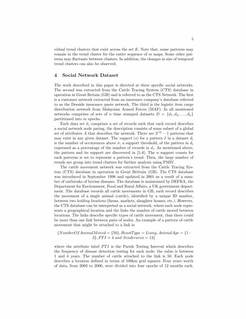
Fig. 1: Schematic illustrating the operation of the proposed framework

Figure 1 gives a schematic of the PMIV framework. The input to the PMIVframework is a set of TC = {τ1, τ2, . . . , τn} partitioned according to m SOMs(note that n should typically be determined by the number of nodes in SOMthat contains groups of similar trends). The set of trends associated with a SOMEj where the complete set of trends, in a sequence of SOM E, is then given byE = {E1, E2, . . . Em}.

The next stage is to detect pattern migrations in the sets of trend clustersTC between k pairs of SOMs Ej and Ej+1, where k = m − 1. This is achievedby generating a sequence of Migration Matrices for each pair. The MigrationMatrices provide the information on members of trend clusters in SOM Ej (mapnode number) moved to trend clusters in SOM Ej+1. This information is used todetermine values the communities of trend clusters and illustrate the animationof pattern migrations using Visuset (Section 6).

The final stage is to illustrate the pattern migration visualisation using Vis-uset. The objective is then to identify interesting of pattern migrations of indi-

5

vidual trend clusters that exist across the set E. Note that, some patterns mayremain in the trend cluster for the entire sequence of m maps. Some other pat-terns may fluctuate between clusters. In addition, the changes in size of temporaltrend clusters can also be observed.

4 Social Network Dataset

The work described in this paper is directed at three specific social networks.The second was extracted from the Cattle Tracing System (CTS) database inoperation in Great Britain (GB) and is referred to as the CTS Network. The firstis a customer network extracted from an insurance company’s database referredto as the Deeside insurance quote network. The third is the logistic item cargodistribution network from Malaysian Armed Forces (MAF). In all mentionednetworks comprises of sets of n time stamped datasets D = {d1, d2, . . . , dn}partitioned into m epochs.

Each data set di comprises a set of records such that each record describesa social network node paring, the description consists of some subset of a globalset of attributes A that describes the network. There are 2|A| − 1 patterns thatmay exist in any given dataset. The support (s) for a pattern I in a dataset diis the number of occurrences above σ, a support threshold, of the pattern in diexpressed as a percentage of the number of records in di. As mentioned above,the pattern and its support are discovered in [5, 6]. The n support counts foreach patterns is set to represent a pattern’s trend. Then, the large number oftrends are group into trend clusters for further analysis using PMIV.

The cattle movement network was extracted from the Cattle Tracing Sys-tem (CTS) database in operation in Great Brittain (GB). The CTS databasewas introduced in September 1998 and updated in 2001 as a result of a num-ber of outbreaks of bovine diseases. The database is maintained by DEFRA, theDepartment for Environment, Food and Rural Affairs, a UK government depart-ment. The database records all cattle movements in GB, each record describesthe movement of a single animal (cattle), identified by a unique ID number,between two holding locations (farms, markets, slaughter houses, etc.). However,the CTS database can be interpreted as a social network, where each node repre-sents a geographical location and the links the number of cattle moved betweenlocations. The links describe specific types of cattle movement, thus there couldbe more than one link between pairs of nodes. An example of a pattern of cattlemovement that might be attached to a link is:

{NumberOfAnimalMoved = {50}, BeastType = Liung,AnimalAge = {1 :3}, PTI = 4 and Senderarea = 13}

where the attribute label PTI is the Parish Testing Interval which describesthe frequency of disease detection testing for each node; the value is between1 and 4 years. The number of cattle attached to the link is 50. Each nodedescribes a location defined in terms of 100km grid squares. Four years worthof data, from 2003 to 2006, were divided into four epochs of 12 months each.

6

After discretisation and normalisation, the average number of nodes within asingle network was 150,000 and the average number of links was 300,000 with445 attributes.

The Deeside Insurance Quote network was extracted from a sample of recordstaken from the customer database operated by Deeside Insurance Ltd. (collab-orators on the work described in this paper). Two years of data, from 2008 to2009, were obtained comprising, on average, 400 records per month. In total, thedata set comprised 250 records with (after discretisation and normalisation) 314attributes. The data was divided into two epochs comprising 12 months each.The Deeside can also be viewed as a network, the nodes comprised postal areas(characterised by the first few digits of UK post/zip codes), and the links arethe number of requests for specific types of insurance quotes received for thegiven time stamp. The Deeside office is viewed as the “super node” that canhave many links to the outlying nodes (customers’ postcodes). An example of apattern of Deeside network, attached to a link, might be:

{CarType = V auxhall, EngineSize = {1500 : 1999}, OffenceCode =SP, F ine = {200 : 500} and Gender = Male}

where the value {1500:1999} states the EngineSize is within the range 1500and 1999, the value SP is an OffenceCode indicating exceeding the speed limit,and the value {200:300} indicates a Fine of between 200 and 500. The averagenumber of records in a single (one month) time stamps was about 800, and theaverage number of links 200.

The MAF Logistic Cargo Distribution dataset described the shipment of lo-gistics items for Malaysian Army, Air Force and Navy. The example of logisticitems were vehicle, medicines, military uniforms, ammunition and repair parts.The dataset was extracted from the 2008 to 2009 records to form 2 episodeswith 12 time stamps each. In the MAF network, logistic items were sent froma number of division logistic headquarters to brigades and then to specific bat-talions in West and East Malaysia. The location of headquarters, brigades andbattalions are the nodes of the MAF network. These offices were viewed as beingsender and receiver nodes (in a similar manner as described for the CTS) andthe shipments as links connecting nodes in the network. Each month comprisedof some 100 records. An example of a pattern of MAF network, attached to alink, might be:

{Item = 1tonnetruck, Sender = 4Armor,Receiver =1Armor, ShipmentCost = {200000 : 500000}}

where the Item described the logistic items that were sent from Sender to Re-ceiver as mentioned in the example. The ShipmentCost described the estimatedtotal cost between MYR200000 and MYR500000 of the cargo distribution fromsender’s location to receiver’s location.

5 Migration Matrices

As mentioned above, the trend clusters are generated from the clustering oflarge numbers of trends into the epochs of SOMs Em. In the Migration Matrices

7

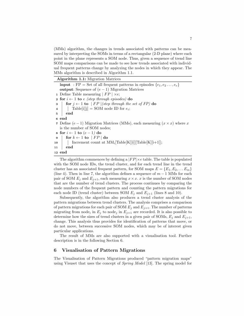
(MMs) algorithm, the changes in trends associated with patterns can be mea-sured by interpreting the SOMs in terms of a rectangular (2-D plane) where eachpoint in the plane represents a SOM node. Thus, given a sequence of trend lineSOM maps comparisons can be made to see how trends associated with individ-ual frequent patterns change by analyzing the nodes in which they appear. TheMMs algorithm is described in Algorithm 1.1.

Algorithm 1.1: Migration Matrices

input : FP = Set of all frequent patterns in episodes {e1, e2 . . . , ee}output: Sequence of (e− 1) Migration Matrices

1 Define Table measuring | FP | ×e;2 for i← 1 to e (step through episodes) do3 for j ← 1 to | FP |(step through the set of FP) do4 Table[i][j] = SOM node ID for ei;5 end

6 end7 Define (e− 1) Migration Matrices (MMs), each measuring (x× x) where x

is the number of SOM nodes;8 for i← 1 to (e− 1) do9 for k ← 1 to | FP | do

10 Increment count at MMi[Table[K][i]][Table[K][i+1]];11 end

12 end

The algorithm commences by defining a |FP |×e table. The table is populatedwith the SOM node IDs, the trend cluster, and for each trend line in the trendcluster has an associated frequent pattern, for SOM maps E = {E1, E2, . . . Em}(line 4). Then in line 7, the algorithm defines a sequence of m− 1 MMs for eachpair of SOM Ej and Ej+1, each measuring x×x. x is the number of SOM nodesthat are the number of trend clusters. The process continues by comparing thenode numbers of the frequent pattern and counting the pattern migrations foreach node ID (trend cluster) between SOM Ej and Ej+1 (lines 8 and 10).

Subsequently, the algorithm also produces a trend cluster analysis of thepattern migrations between trend clusters. The analysis comprises a comparisonof pattern migrations for each pair of SOM Ej and Ej+1. The number of patternsmigrating from nodei in Ej to nodej in Ej+1 are recorded. It is also possible todetermine how the sizes of trend clusters in a given pair of SOMs, Ej and Ej+1,change. This analysis thus provides for identification of patterns that move, ordo not move, between successive SOM nodes, which may be of interest givenparticular applications.

The result of MMs are also supported with a visualisation tool. Furtherdescription is in the following Section 6.

6 Visualisation of Pattern Migrations

The Visualisation of Pattern Migrations produced “pattern migration maps”using Visuset that uses the concept of Spring Model [13]. The spring model for

8

drawing graphs in 2-D space is designed to locate nodes in the space in a mannerthat is both aesthetically pleasing and limits the number of edges that cross overone another. The graph to be depicted is conceptualised in terms of a physicalsystem where the edges represent springs and the nodes objects connected bythe springs. Nodes connected by “strong springs” therefore attract one anotherwhile nodes connected by “weak springs” repulse one another. The graphs aredrawn following an iterative process. Nodes are initially located within the 2Dspace using a set of (random) default locations (defined in terms of an x andy coordinate system) and, as the process proceeds, pairs of nodes connected bystrong springs are “pulled” together. In the context of PMIV The network nodesare represented by the trend clusters in SOM E and the spring value was definedin terms of a correlation coefficient (C):

Cij =X√

(|Eki| × |Ek+1j |)(1)

where Cij is the correlation coefficient between a node (trend cluster) i in SOMEk and a node j in SOM Ek+1 (note that i and j can represent the same nodebut in two different maps), X is the number of trend lines that have movedfrom node i to j and |Eki| (|Ek+1j |) is the number trends at node i (j) in SOMEk (Ek+1j). A migration is considered “interesting”, and thus highlighted byVisuset, if C is above a specified minimum relationship threshold (Min-Rel).With respect to all network we have discovered that a threshold of 0.2 is a goodworking Min-Rel value. The Min-Rel value is also used to prune links and nodes;any link whose C value is below the Min-Rel value is not depicted.

To aid the further analysis of the identified pattern migrations it was alsoconsidered desirable to identify “communities” within networks (SOM E), i.e.clusters of nodes which were “strongly” connected (feature significant migration).This would indicate significant groupings of patterns whose associated trend lineswhere changing between SOM Ek and Ek+1. An agglomerative hierarchical clus-tering mechanism, founded on the Newman method [16] for identifying clustersin network data, was therefore adopted. Newman proceeds in the standard it-erative manner on which agglomerative hierarchical clustering algorithms arefounded. The process starts with a number of clusters equivalent to the num-ber of nodes. The two trend clusters (nodes) with the greatest “similarity” arethen combined to form a merged cluster. The process continues until a “best”cluster configuration is arrived at or all nodes are merged into a single cluster.The overall process is typically conceptualised in the form of a dendrogram. Bestsimilarity is defined in terms of the Q-value, this is a “modularity” value whichis calculated as follows:

Qi =

i=n∑i=1

(cii − a2i ) (2)

where Qi is the Q-value associated with the current node i, n is the total numberof nodes in the network, cii is the fraction of intra-cluster (within cluster) links(trend lines) in cluster i over the total number of links in the network, and a2i is

9

the fraction of links that end in the nodes in cluster i if the edges were attachedat random. The value ai is calculated as follows:

ai =

j=n∑j=1

cji (3)

where cij is the fraction of inter-cluster links, between the current cluster i andthe cluster j, over the total number of links in the network.

In this paper, the implementation of Visuset, trend clusters are depicted assingle nodes that might have self-links of pattern migrations within the sametrend clusters themselves, node pairs linked by an edge, chains of nodes linkedby sequence of edges or “islands” of nodes that represent as communities ofnodes. This will be demonstrated in Section 7.

7 Analysis of PMIV using Social Network Trend Clusters

Each of the three network is considered in turn in this section. Table 1 providesnumber of trends and trend clusters for CTS, Deeside Insurance and MAF CargoDistribution networks. The support threshold (σ) used to mine frequent patternsand trends for CTS network is 0.5%, and Deeside Insurance and MAF LogisticCargo networks is 5%. The trend clusters are discovered, for all networks, usingSOM. The number of nodes that consist of trends in SOMs determines thenumber of trend clusters. Therefore, CTS network has 100 trend clusters, DeesideInsurance and MAF Cargo Distribution networks have 49 trend clusters. CTSnetwork had the biggest SOM node configuration as it is the largest datasetcompared to the other two networks.

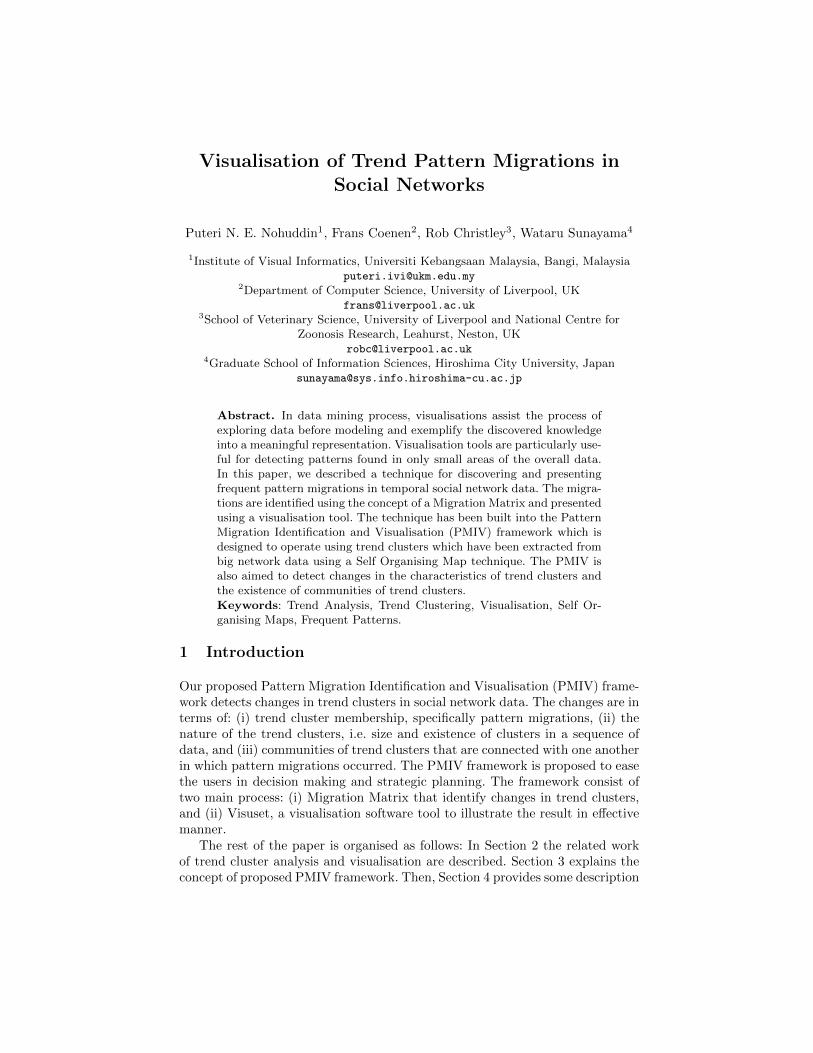
Then, the trend clusters are processed using MMs algorithm to idetify thenumber of pattern migrations in each pair of SOM Ej and Ej+1, a genericexample is shown in Table 2. The table shows a MM that provides the numbersof CTS patterns that have migrated from E2003 to E2004, n1,1 = 71, the numberof patterns that have stayed (self-links in cluster c1 in both SOM maps , n1,2= 13, the number of CTS patterns that have migrated from c1 in E2003 to c2in E2004. The Q-values required for the hierarchical clustering are calculatedusing these numbers of pattern migrations. The numbers of patterns migratedin the Table 2, are also used to determine the Q and C-values for visualising thepattern migrations. These Q-values are used to cluster the nodes (trend clusters)so as to detect communities of nodes with pattern migrations. As mentioned, theC-values were used to identify the positions and relationships of trend clusternodes in the network to support the animation of pattern migrations. SimilarMMs were also generated for Deeside Insurance and MAF Cargo Distributionnetworks

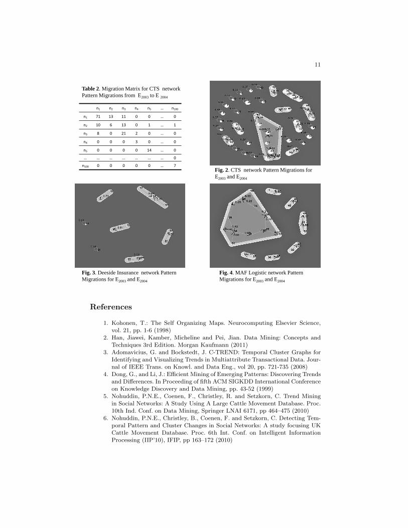
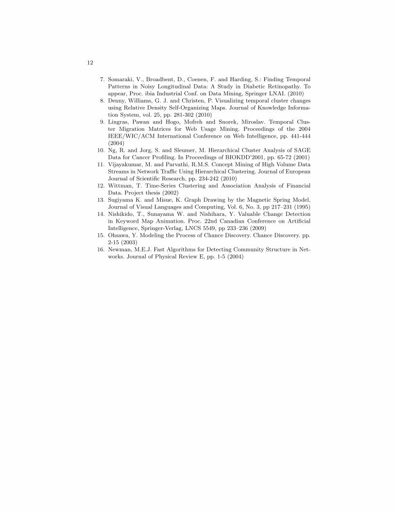
In the second process, Visuset took the generated MMs to illustrate thepattern migration maps. The maps for all three networks are shown in Figure2, 3 and 4. Note that, in the maps, trend clusters are represented as nodes andmigrations of patterns are shown as links. The C-values threshold for patternmigrations between nodes is above 0.2.

10

Table 1: Number of trend clusters for CTS, Deeside Insurance and MAF Cargo Distri-bution networks

Networks Support Trends Trends Number of

Threshold σ (%) in Ej in Ej+1 Trend Cluster

CTS 0.5 63117 66870 100Deeside Insurance 5 55241 49983 49MAF 5 3491 2609 49

Figure 2 shows that the CTS network pattern migration map between E2003

and E2004 with 45 nodes out of a total of 100 that had a C-value greater than0.2. Several islands are displayed, determined using the Newman method de-scribed above, including a large island comprising eight nodes. The islands indi-cate communities of pattern migrations. The nodes are labeled with an identifier(the trend cluster number in Ej), the links with their C-value numbers and linkdirections show the migration of patterns to new trend cluster in Ej+1. Fromthe map we can identify that there are a 30 nodes, of self-links. However, we candeduce that (for example) patterns are migrating from node 34 to node 44, andfrom node 44 to 54 (thus indicating a trend change). The size of the nodes alsoindicates how many patterns in the cluster, bigger node has large patterns in it.

Figure 3 depicts the Deeside network pattern migration map between E2008

and E2009. There were 13 nodes that have C-value greater that 0.2. Note thatthe node 28 has C-value of 0.69, the highest pattern migrations to the node36 in E2009. There were also self-links occurred for only two node, 19 and 21.We can also notice that the size of nodes 19 24, 28 and 32 were among thelargest which means the number of cluster members was high compared to otherclusters. There were five islands of nodes in which nodes 24, 30 and 31 formedthe largest island in the map.

Finally, the pattern migrations map for MAF Cargo Distribution network isshown in Figure 4. There 24 nodes out of 49 were shown in the map. Unlikethe other maps, the network did not have any self-link pattern migrations. Themap also had seven islands of nodes, the largest island has about 12 nodes thatconnected to one another for pattern migrations. The were also some nodesreceived new cluster members in E2009 such as node 10, 26 and 34.

8 Conclusions

In this paper, the authors have described the PMIV framework for detectingchanges in trend clusters within social network data. The trend clusters consistof trends are defined in terms of sequences of support counts associated withindividual patterns across a sequence of time stamps associated with an epoch.The trend clusters are analysed for identifying pattern migrations between pairsof trend clusters found in SOM Ej and Ej+1. The pattern migrations are detectedusing the Migration Matrices algortihm and Visuset, a visualisation softwaretool. Visuset in PMIV provides useful information: (i) pattern migrations oftrend cluster (membership), (ii) changes in trend clusters, and (iii) communitiesof trend clusters of pattern migrations.

11

n1 n2 n3 n4 n5 … n100

n1 71 13 11 0 0 … 0

n2 10 6 13 0 1 … 1

n3 8 0 21 2 0 … 0

n4 0 0 0 3 0 … 0

n5 0 0 0 0 14 … 0

… … … … … … … 0

n100 0 0 0 0 0 … 7

Table 2. Migration Matrix for CTS network

Pattern Migrations from E2003 to E 2004

Fig. 2. CTS network Pattern Migrations for

E2003 and E2004

Fig. 4. MAF Logistic network Pattern

Migrations for E2003 and E2004

Fig. 3. Deeside Insurance network Pattern

Migrations for E2003 and E2004

References

1. Kohonen, T.: The Self Organizing Maps. Neurocomputing Elsevier Science,vol. 21, pp. 1-6 (1998)

2. Han, Jiawei, Kamber, Micheline and Pei, Jian. Data Mining: Concepts andTechniques 3rd Edition. Morgan Kaufmann (2011)

3. Adomavicius, G. and Bockstedt, J. C-TREND: Temporal Cluster Graphs forIdentifying and Visualizing Trends in Multiattribute Transactional Data. Jour-nal of IEEE Trans. on Knowl. and Data Eng., vol 20, pp. 721-735 (2008)

4. Dong, G., and Li, J.: Efficient Mining of Emerging Patterns: Discovering Trendsand Differences. In Proceeding of fifth ACM SIGKDD International Conferenceon Knowledge Discovery and Data Mining, pp. 43-52 (1999)

5. Nohuddin, P.N.E., Coenen, F., Christley, R. and Setzkorn, C. Trend Miningin Social Networks: A Study Using A Large Cattle Movement Database. Proc.10th Ind. Conf. on Data Mining, Springer LNAI 6171, pp 464–475 (2010)

6. Nohuddin, P.N.E., Christley, B., Coenen, F. and Setzkorn, C. Detecting Tem-poral Pattern and Cluster Changes in Social Networks: A study focusing UKCattle Movement Database. Proc. 6th Int. Conf. on Intelligent InformationProcessing (IIP’10), IFIP, pp 163–172 (2010)

12

7. Somaraki, V., Broadbent, D., Coenen, F. and Harding, S.: Finding TemporalPatterns in Noisy Longitudinal Data: A Study in Diabetic Retinopathy. Toappear, Proc. ibia Industrial Conf. on Data Mining, Springer LNAI. (2010)

8. Denny, Williams, G. J. and Christen, P. Visualizing temporal cluster changesusing Relative Density Self-Organizing Maps. Journal of Knowledge Informa-tion System, vol. 25, pp. 281-302 (2010)

9. Lingras, Pawan and Hogo, Mofreh and Snorek, Miroslav. Temporal Clus-ter Migration Matrices for Web Usage Mining. Proceedings of the 2004IEEE/WIC/ACM International Conference on Web Intelligence, pp. 441-444(2004)

10. Ng, R. and Jorg, S. and Sleumer, M. Hierarchical Cluster Analysis of SAGEData for Cancer Profiling. In Proceedings of BIOKDD’2001, pp. 65-72 (2001)

11. Vijayakumar, M. and Parvathi, R.M.S. Concept Mining of High Volume DataStreams in Network Traffic Using Hierarchical Clustering. Journal of EuropeanJournal of Scientific Research, pp. 234-242 (2010)

12. Wittman, T. Time-Series Clustering and Association Analysis of FinancialData. Project thesis (2002)

13. Sugiyama K. and Misue, K. Graph Drawing by the Magnetic Spring Model,Journal of Visual Languages and Computing, Vol. 6, No. 3, pp 217–231 (1995)

14. Nishikido, T., Sunayama W. and Nishihara, Y. Valuable Change Detectionin Keyword Map Animation. Proc. 22nd Canadian Conference on ArtificialIntelligence, Springer-Verlag, LNCS 5549, pp 233–236 (2009)

15. Ohsawa, Y. Modeling the Process of Chance Discovery. Chance Discovery. pp.2-15 (2003)

16. Newman, M.E.J. Fast Algorithms for Detecting Community Structure in Net-works. Journal of Physical Review E, pp. 1-5 (2004)