G

Visual Tracking by Sampling in Part Space Lianghua Huang, Bo Ma, Member, IEEE, Jianbing Shen, Senior Member, IEEE, Hui He,

Ling Shao, Senior Member, IEEE, and Fatih Porikli, Fellow, IEEE

Abstract— In this paper, we present a novel part-based visual tracking method from the perspective of probability sampling. Specifically, we represent the target by a part space with two

online learned probabilities to capture the structure of the target. The proposal distribution memorizes the historical performance of different parts, and it is used for the first round of part selec-

tion. The acceptance probability validates the specific tracking stability of each part in a frame, and it determines whether to accept its vote or to reject it. By doing this, we transform the

complex online part selection problem into a probability learning one, which is easier to tackle. The observation model of each part is constructed by an improved supervised descent method

and is learned in an incremental manner. Experimental results on two benchmarks demonstrate the competitive performance of our tracker against state-of-the-art methods.

Index Terms— Visual tracking, part space, sampling.

I. INTRODUCTION

IVEN a specified object in the first frame, the task

of visual tracking is to locate it in the succes-

sive video frames. As a fundamental topic in com-

puter vision, object tracking plays an important role in

numerous applications such as visual surveillance, human-

computer interaction and augmented reality. Despite decades

of studies [1], [35], [41], [46], visual tracking is still a chal-

lenging task due to target appearance variations such as object

deformation, occlusion, illumination changes, motion blur and

background clutters.

For object tracking, local appearance models [5], [7], [8]

are generally more robust than holistic ones [4], [6], since

many challenging factors, e.g., the object deformation and

This work was sup- ported in part by the National Natural Science Foundation of China under Grant 61472036, in part by the National Basic Research Pro- gram of China (973 Program) under Grant 2013CB328805, and in part by the Australian Research Council’s Discovery Projects Funding Scheme under Grant DP150104645. Specialized Fund for Joint Build- ing Program of the Beijing Municipal Education Commission. The asso- ciate editor coordinating the review of this manuscript and approv- ing it for publication was Prof. Ce Zhu. (Corresponding author: Bo Ma.)

L. Huang, B. Ma, J. Shen, and H. He are with the Beijing Laboratory of Intelligent Information Technology, School of Computer Science, Beijing Institute of Technology, Beijing 100081, China (e-mail: bma000@bit.edu.cn; shenjianbing@bit.edu.cn).

L. Shao is with the School of Computing Sciences, University of East Anglia, Norwich NR4 7TJ, U.K. (e-mail: ling.shao@ieee.org).

F. Porikli is with the Research School of Engineering, The Australian National University, Canberra, ACT 0200, Australia (e-mail: fatih.porikli@anu.edu.au).

partial occlusions, can be viewed as local noise or variations.

Numerous local appearance models have been proposed in

recent years and have achieved promising results. Existing

methods can be roughly categorized into the following classes:

sparse representation based methods [7]–[9], [22], segmenta-

tion based methods [5], [26], [29], pooling methods [10], [11]

and part-based methods [12], [20], [44].

Sparse representation based methods work under the

assumption of sparse noise (e.g., partial occlusions and local

background clutter), and represent the target as a sparse com-

bination of templates and noisy pixels [8], [9]. Despite their

effectiveness in handling occlusions and background noise,

they are not suitable for tackling deformable objects, where

the shifted parts will be mistakenly regarded as noise. Seg-

mentation based methods [5] separate the target and the back-

ground into several irregular patches (e.g., superpixels), and

formulate tracking as an online segmentation or patch classi-

fication problem. The flexibility of these methods makes them

handle partial occlusions and object deformation robustly.

However, it is still difficult for them to obtain accurate bound-

ing boxes. Besides, the segmented patches are not uniform

in size, which makes them difficult to generalize. Pooling

methods [10], [11], [43] obtain local patches from the target

by performing sliding windows on it, and represent the target

with pooled features of local descriptors. These methods

can decrease the impact of local noise. Nevertheless, when

variations of large areas exist, such as object deformation and

severe occlusions, the noisy blocks will have negative impact

on target locating.

When an object deforms or suffers from occlusions, its

holistic appearance changes a lot, but part of its local

appearance remains identifiable. Based on this idea, part-

based models have been introduced in many computer vision

tasks [12], [14]–[17], [44]. In object detection [45], [47],

deformable part models (DPM) [14] has been proposed and

achieved state-of-the-art performance. Subsequently, it attracts

popularity and numerous improvements to DPM have been

presented [15]–[17]. In visual object tracking, part-based mod-

els have also been proposed to deal with target deformation

and partial occlusions [12], [20], [44], [48]. Yao et al. [12]

presented a part-based tracking method with online latent

structured learning. This work can be viewed as an online

extension of DPM in visual tracking. In [44], a part-based

tracking method with cascaded regression was proposed,

which exploits the spatial constraints between parts to learn the

intrinsic shape of an object. Lu et al. [20] proposed an online

tracking-learning-parsing framework that utilizes an and-or

graph to capture the construction of objects.

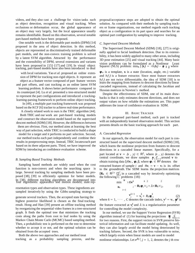
Fig. 1. Illustration of the proposed part-based tracking algorithm. A part space of the target is initialized in the first frame according to the proposal distribution α. Then α is updated in each frame based on the contributions of parts to target locating. We sample parts according to α and track them independently. Votes of different parts are accepted/rejected according to an acceptance probability β, then the target location is estimated based on the accepted votes.

Although above trackers have made attempts to apply the

part-based strategy in visual tracking, the part-based methods

for tracking are far less popular than for object detection.

One of the main reasons is the lack of training samples

with the tracking data. For object detection, there are enough

samples for determining the best way of part separation.

However, for object tracking, the only information provided is

the target location in the first frame. It is difficult to determine

how the target is separated with only one sample of an object.

A better way is to learn the separations online. However,

an online part separation model is usually complex and time

consuming.

We propose a new part-based method to solve the above

issues from the perspective of probability sampling. The

overview of our method is illustrated in Fig. 1. We represent

each target by a part space, which contains sufficient regions

to cover most structures of objects, and two online learned

probabilities on it - the proposal distribution α and the

acceptance ratio β. The α represents the historical information

of different parts and is applied on the first round of part

selection, while the β validates the frame specific tracking

stability of each part and determines whether to accept a part’s

vote to the target location or not. Thus, the complex online part

selection problem is transformed into a probability learning

one, which is much easier to solve. The observation model of

each part is constructed by an improved supervised descent

method (SDM) [18], where we incorporate the basic SDM

model with a confidence evaluation scheme for indicating the

reliability of each predicted descent direction. We propose

an incremental cascaded support vector regression (ICSVR)

algorithm for model updating. To recover the unselected parts,

we further present a part relocating scheme. Our source code

will be available online.1

Compared to the existing approaches, the proposed visual

tracking method provides the following contributions:

• We propose a novel part-based method, which represents

each target by a part space and two learned probabilities,

to transform the complex online part selection problem

into a probability learning one.

• An improved supervised descent method (SDM) is pro-

posed to construct the observation model of each part,

which incorporates the basic SDM model with a confi-

dence evaluation scheme for indicating the reliability of

each predicted descent direction.

• To achieve robust visual tracking, we further propose an

incremental cascaded support vector regression (ICSVR)

algorithm for model updating and an unselected relocat-

ing scheme for parts updating.

II. RELATED WORKS

In this section, we briefly review three closely related topics:

part-based models, sampling based tracking methods and the

supervised descent methods.

A. Part-Based Models

Partial occlusions, background noise and object deformation

are some of the most common phenomena in real world

1http://github.com/shenjianbing/partspacetrack

2

{ i }

k=1

i

{ k}

videos, and they also cast a challenge for vision tasks such

as object detection, recognition and visual tracking. When

occlusions or deformation occur, the global appearance of

an object may vary largely, but the local appearance usually

remains identifiable. Based on this observation, several notable

part-based methods have been proposed.

One notable work is the deformable part models (DPM) [14]

proposed in the area of object detection. In this method,

objects are represented as discriminatively trained deformable

part models, and the non-convex training problem is solved

by a latent SVM algorithm. Attracted by the performance

and the extensibility of DPM, several extensions and variants

have been proposed in [15]–[17] and [19]. In visual object

proposal/acceptance steps are adopted to obtain the optimal

solution. As compared with their methods by sampling track-

ers or frame organizations, our method regards each tracking

object as a configuration in its part space and searches for an

optimal part configuration by sampling to improve tracking.

C. Supervised Descent Methods

The Supervised Descent Method (SDM) [18], [27] is origi-

nally applied to facial landmark detection. Due to its extensi-

bility, it has been widely applied to many other areas, including

3D pose estimation [25] and visual tracking [44]. Many basic

vision problems can be formulated as a Nonlinear Least Squares (NLS) problem: minx f (x) = ×h(x) − φ × , where

tracking, part-based models have also been introduced to deal ∗ 2

with local variations. Yao et al. proposed an online exten-

sion of DPM for tracking non-rigid objects. It represent an

object as a feature vector composed of part feature vectors

and part offsets, and cast tracking as an online latent SVM

learning problem. It shows better performance compared to

its counterpart [4]. Lu et al. presented a tree-structured model

to represent the part configurations and introduced a tracking-

learning-parsing framework to perform online object tracking.

In [49], a multiple part tracking framework was proposed

based on the KCF [6] tracker to achieve real-time performance.

A closely related work to ours is the TRIC algorithm [44].

Both TRIC and our work are part-based tracking models

and construct the observation model based on the supervised

descent method (SDM) [18]. However, the differences between

them are obvious. First, our method aims at learning the best

way of part selection, while TRIC is conducted to build a shape

model for a target and it performs no part selection. Second,

our method tracks each part independently and combine their

results in postprocessing steps. Instead, TRIC locates each part

based on its three adjacent parts. Third, we have improved the

SDM by introducing an confidence evaluation scheme.

B. Sampling Based Tracking Methods

Sampling based methods are widely used when the cost

function is non-convex and when the searching space is

large. Several tracking by sampling methods have been pro-

posed [38], [39] to efficiently optimize for better models.

In [38], different tracking algorithms are decomposed into four ingredients: appearance and motion models, state rep-

φ∗ is a template, x is a state (location, angle, etc.) variable

and h(·) is a feature extractor. Since most feature extractors

h(·) are not twice differentiable, the idea of SDM [18] is to learn the mapping from features to descent directions by linear

cascaded regressions, instead of calculating the Jacobian and

Hessian matrices in Newton’s method.

Despite the effectiveness of SDM, one of its main draw-

backs is that it only estimates descent directions, and does not

output values on how reliable the estimations are. This paper

addresses the issue of confidence evaluation in SDM.

III. BASIC TRACKER

In the proposed part-based method, each part is tracked

with an independently learned observation model. This section

presents details on the basic tracking approach for each part.

A. Cascaded Regression

In our approach, the observation model for each part is con-

structed based on the supervised descent method (SDM) [18],

which learns the nonlinear projection from features to descent

directions in a cascaded linear manner. Specifically, for a

part located at v = (x , y) ∈ R2, where (x , y) denotes the central coordinate, we draw samples v n around v to

i=1

obtain training data {(6vi , φi )}, where φi ∈ Rp denotes the

extracted feature of sample i and 6vi = v − vi is its offset to the groundtruth. The SDM learns the projection matrices

{Rk ∈ R2× p}C in a cascaded way by iteratively optimizing the following C problems [18]:

n min .

×6vk k 2 2

resentation types and observation types. These ingredients are

sampled iteratively by using the Gibbs sampling strategy to

Rk

i=1

i − Rk φi ×2 + λ×Rk ×2, (1)

vk+1 k k

generate several trackers. Then, the accepted state having the

highest posterior likelihood is chosen as the final tracking

i = vi + Rk φi , (2) where k = 1, · · · , C denotes the cascade index, v1 = vi , φ

k is i i

result. Hong and Han [39] present an offline tracking method

by reorganizing the sequential video frames in a tree-structured

graph. It finds the optimal tree that minimizes the tracking

costs along the paths from root to leaf nodes by using the

Markov Chain Monte Carlo (MCMC) based sampling method.

Then, a probabilistic test is performed on the tree to determine

whether to accept it or not, and the optimal solution can be

obtained from the accepted trees.

Both the above two approaches and our method treat

tracking as a probability sampling process, and the

the feature extracted at vk and λ is a regularization parameter

for controlling the model complexity.

In our method, we use the Support Vector Regression (SVR)

algorithm instead of (1) for learning the projections R C k=1

for two reasons. First, the support vectors in SVR preserve his- torical information and can facilitate model updating. As well,

they can also largely avoid the model being deteriorated by

tracking failures. Second, the SVR is less vulnerable to noise,

which largely exists when linear models are used to model

nonlinear relationships. Let r(kj ), j = 1, 2, denotes the j th row

2σ 2

∗

k=1

2 i=1

2 i

i

i

i

∗

i

i

i=1

i

i

.

of Rk , 6v(kj )

denotes the j th entry of 6vk, and the cascaded In our method, the dominant set algorithm [28] is adopted i

SVR is then formulated as:

1 2

i

n .

(kj )

∗(kj )

to seek for the voting center. The dominant set algorithm

computes the weight wi for each sample by optimizing: min

r(k j ),ξ (k j ),ξ ∗(k j ) ×r(kj )×2 + η1

i=1

(ξi + ξi ), max w

wTAw,

s.t. (r(kj ) · φk ) − 6v(kj )

≤ ε1 + ξ (kj )

, s.t. w ∈ α, (7) i i

6v(kj )

i ∗(kj ) where α = {w ∈ Rm : w ≥ 0 and eTw = 1}, e ∈ Rm

i − (r(kj ) · φk

i

ξ (kj )

∗(kj ) i ) ≤ ε1 + ξ ,

is a vector of all 1s, A ∈ R m×m 2

is an affinity matrix with

i , ξi ≥ 0, i = 1, · · · , n, k = 1, · · · , C, (3)

each entry A ij = exp (− ×v i −v j ×2 ) representing the similarity

A

where η1 is a regularization factor, ξ (kj )

, ξ ∗(kj )

are slack between v i and v j , σA is a scaling factor. As noted in [28], i i σA is set to be the median value of all entries in A. Finally,

variables and ε1 is a pre-set margin. We set ε1 = 5, which means the allowed prediction bias without punishment is

5 pixels.

the part is located by:

v =

m . i=1

wi v i . (8)

B. Confidence Evaluation

Despite the effectiveness of SDM, its main drawback is

the lack of a mechanism for indicating how reliable an

offset prediction is. In this section, we present a confidence

evaluation scheme for SDM.

In the training stage, if one regress iteration pulls a sample

closer to the groundtruth, we say that the sample is more

credible and vice versa. Based on the idea, we propose to

Taking the sample confidence ci into consideration,

we slightly modify the affinity matrix A as:

Aij = ci · c j · Aij . (9)

The rest of the voting process is the same as described before.

D. Updating Scheme

learn an extra set of projection matrices {Qk ∈ R1× p}C for confidence evaluation. We take the ratio of overlap rates before and after regression θ k = (ok+1)2/ok (where ok denotes the

To adapt the basic model to part appearance variations,

we propose an Incremental Cascaded Support Vector Regres-

sion (ICSVR) algorithm for model updating. To deduce the i i i i

overlap between vk and v) as the label to train {Qk }C : i k=1

n

updating scheme, we first investigate the relationship between

Support Vector Classification (SVC) and Support Vector

min 1

×Qk ×2 + η2 .

(ξ (k) + ξ ∗(k)), Regression (SVR). With training data {xi , yi }h , the SVR

Qk ,ξ (k),ξ ∗(k) 2 i i

i=1 problem can be formulated as:

s.t. Qk · φk − θ k ≤ ε2 + ξ (k)

, 1 h

i i

θ k k i (k) min

2 ×w×2 + η (ξi + ξ ∗),

i − Qk · φi ≤ ε2 + ξ ∗

w,ξ ,ξ ∗ i=1

ξ (k) ∗(k) s.t. (w · x ) − y ≤ ε + ξ ,

i , ξi ≥ 0,

i = 1, · · · , n, k = 1, · · · , C. (4)

We set ε2 = 1, which is comparable with the magnitude of θ k. During testing, with the estimated {θk = Qk · φk }C for each

i i i

yi − (w · xi ) ≤ ε + ξ ∗,

ξi , ξi ≥ 0, i = 1, · · · , h, (10)

where η is a regularization parameter, ε is a pre-set margin i i

sample, the credibility ci is then computed as:

C

k=1 and ξi , ξ ∗ are slack variables.

The above problem is equivalent to a Support Vector ci =

θk , k = 1, · · · , C. (5) Classification model formulated on the modified training data i h 2h T T

k=1 {(zi , 1)}i=1 and {(zi , −1)}i=h+1, where zi = (xi , yi + ε) for

C. Part Locating

i = 1, · ·· , h and zi = (xT, yi − ε)T for i = h + 1, · ·· , 2h: 2h

The motion model of our method is based on the particle

filters framework [13]. When locating a part in a new frame, min w,ξ

1 w 2

2 × ×2 +

η .

ξi ,

i=1

we sample around its last estimated position v from Gaussian distribution N (v, €2), where €2 = diag(r2, r2), to obtain

s.t. (w · zi ) ≥ 1 − ξi , i = 1, · · · , h, (w · zi ) ≥ 1 − ξi , i = h + 1, ·· · , 2h,

m candidates {vi , φi }m . With the learned cascaded model, we iteratively pull each sample vi to the estimated part location

from a start state v1:

vk+1 k k

i = vi + Rk φi , k = 1, · · · , C, (6)

After C iterations, we obtain all the estimated states v i = vC

+1. Intuitively, the most densely voted location is more likely to

be the part location.

−

ξi ≥ 0, i = 1, ·· · , 2h, (11)

where η is a regularization parameter.

In this case, the online learning of SVR can be implemented

by online SVC algorithms with slightly modified training data.

We use the twin prototypes algorithm [30] in [3] as the SVC

updater in our approach. In the twin prototypes algorithm,

the SVC model can be compactly summarized as a prototype

2

i=1

j =1

2

k=1

c=0 s

.L l 1

l .L

1

J

2

set {ψi , ςi , si }B , where ψi is a feature vector, ςi is a binary

label and si is a counting number that indicates how many support vectors are represented by this instance. With new data

{z j ,γ j }J , where z j is a feature vector and γ j is a binary label, the SVC model is updated by minimizing:

B

min 1

×w× + K ( .

si Lh (ςi , ψi ; w) w,b 2 B

i=1 1 .

+ J

j =1

Lh (z j ,γ j ; w)) (12)

where Lh is the hinge loss.

After training, support vectors from the new data are added

to the prototype set with counting number 1. When the size of the prototype set is larger than a predefined budget B , the pair

of prototype instances of the same label with the mimimal

distance are merged into (ψ∗,ς ∗, s∗), where si1

ψi1 + si2

ψi2 ∗ ∗

ψ∗ = si1 + si2

, ς = ςi1 , s = si1 + si2 . (13)

Fig. 2. Illustration of part space in sequence Woman. For clarity, we only

In our experiments, we use B = 80 as the budget and K = 100 for weighting the loss term, though we found that our tracking

performance tends to be insensitive to these settings.

Finally, we extend the online SVR to the cascaded version. After tracking in each frame, we draw samples {6v1, φ1}I

show the parts that are no bigger than half of the object size. Boxes in blue and yellow denote parts of different sizes. The red boxes denote the tracking results. (a) Part space in frame #16. (b) Part space in frame #70. (c) Part space in frame #128. Due to occlusion, the bottom blue and yellow parts drift away from the target. (d) The occluded parts are relocated in frame #168.

i i i=1 .L

around the estimated part location v from Gaussian distribution is served as a proposal distribution and l=1 αl = 1. When

N (v, €1), where €1 = diag(r1, r1), to obtain training data for the first cascade. Then each sample is iteratively updated as:

v k+1 k k

i = vi + Rk φi . (14)

locating the target, we first sample Lα = 5 parts from the part space according to α without replacement, and then track each

one independently with its observation model.

After tracking, the confidences for different parts are The samples {6vk, φk }I

, k = 2, ··· , C are then collected obtained and normalized to calculate the acceptance ratio i i i=1 L

for the updating of the kth cascade, where 6vk = v − vk. β ∈ R where βl ∈ [0, 1]. The β examines the tracking result i i

IV. TRACKING BY SAMPLING IN PART SPACE

As described in Section III, the observation model for each

part is represented by a set of projection matrices {Rk , Qk }C . This section presents details on the online selection and updat-

ing of these parts, and how to use them for target locating.

A. Part Space

In our implementation, the initial parts are automatically

generated based on the bounding box (x , y, width, height) of

the tracking target in the first frame. Specifically, we separate

the bounding box into two parts equally along the long side.

For each part, we perform the same partition process to obtain

of each part in the current frame and determines whether to

accept its vote to the target location.

With the accepted parts, the target is located with their votes

by using the dominant set algorithm. The online learning of

probabilities α and β and the relocating of unaccepted parts

are described in the following sections.

B. Part Selection

1) Proposal Distribution: The proposal distribution α ∈ RL

evaluates the contributions of different parts over time and

is used for the first round of part selection. Denote s as the

estimated target location in a frame and sl , l = 1, · · · , L as the votes from parts. We define the contribution gl of a part to target locating as:

another pair. After P iterations, L = .P

2c parts are sl ×2

obtained. We set P = 2 in our experiments, which generates gl = exp (− ׈ −ˆ

), (15)

L = 7 parts (as illustrated in Fig. 2). These parts make up the ‘part space’ in our approach. Since the main idea of our approach is to transform the complex online part selection problem to a probability learning one, the roughly selected

2(σ1)2

where σ1 is the scaling factor and is set to 4 pixels, which is

comparable with the allowed prediction bias. The normalized contribution vector g is calculated as: gl =

regions are enough for it to work well. Though, we believe

our method can be easily extended with automatic initial parts,

gl

l=1 gl

so that .L

= gl = 1. The initial α(1) is set as the

such as region proposal for the initial bounding boxes. During

tracking, a probability α ∈ RL on the part space is learned online to memorize the contributions of different parts, which

normalized part areas:

α(1) = Sl

l=1 Sl

, (16)

( pi ) β

i = v

2

0

Algorithm 1 The Proposed TPS Tracker

Fig. 3. Overall performance of 31 state-of-the-art trackers and our tracker on OTB-100 and CVPR2013. For clarity, only top 10 trackers are displayed. (a) Results of OPE on OTB-100. (b) Results of OPE on CVPR2013.

By normalizing the voting stability τ , we obtain the accep-

tance ratio:

τ β = .n

i=1

. (19)

where Sl denotes the area of part l and the superscript (1)

denotes the frame index. This is consistent with the intuition

that larger parts are more recognizable.

Afterwards, the α(t ) is updated as:

α(t ) = μα(t −1) + (1 − μ)g (t ), t = 2, · · · , T , (17)

We denote βl as the acceptance ratio for part l. The vote

of part l on the target location is accepted at the probability

βl . To avoid the situation that no parts are accepted, we set a

minimum number as Lmin = 3. When the number of accepted parts Lβ is less than Lmin , we repeat the process until it is larger than Lmin .

C. Locating and Relocating

With Lβ accepted parts (denote the indexes as p1, ··· , pLβ )

where g (t ) is the contribution vector in the t-th frame and μ and their estimated states {v L

}i=1, their votes to the target is a forgetting factor fixed at 0.9 in our experiments. can be obtained with the part offsets:

2) Acceptance Probability: The probability βl ∈ [0, 1], l = 1, ··· , L emphasizes the frame specific tracking perfor-

s p ( pi ) + 6v

( pi ) , (20)

mance of a part, which is served as an acceptance ratio. The

basic observation is, if a part is being occluded or disturbed

by background noise, its candidate votes (see Section III-C)

will be scattered, otherwise densely distributed. Based

on this idea, we define the voting stability τ for each

part as:

where 6v( pi ) = s − v( pi ) denotes the offset between the target state s and the groundtruth location of part pi , and it is calculated in the first frame. Similar to Section III-C,

we calculate the weight for each vote wi with the dominant

set algorithm [28]. Finally, the target is located as:

Lβ . n

vi v× s = wi s pi . (21) τ = .

ci exp (− ׈ −ˆ

2 ), (18) i=1

i=1 2(σ2)2

For the unaccepted parts (denote the indexes as q1, ··· , qLq

where Lq = L − Lβ ), we need to relocate them according to where v is the voting center, v i denotes the estimation of the i th candidate (see Section III-C), ci is the confidence value as

described in Section III-B and σ2 is a scaling factor fixed to 3 pixels, which approximates the radius of candidate votes in

dense areas.

the estimated target location in the current frame.

First, we pull these parts to the corresponding anchor points

on the target:

v(qi ) = s − 6v(qi ), i = 1, ·· · , Lq . (22)

ci

0

0 (qi )

0

×2

Fig. 4. The success plots of videos with different attributes on OTB-100. The number in the title indicates the number of sequences.

Then, for each part, starting from v(qi ), we locate it with

its observation model as described in Section III-C to obtain

stage, we sample 200 images around the estimated position for

each part with sample radius r1 = 8. We train C = 3 cascades the estimated state v (qi ). Denote ρi = ×v

(qi ) − v 2 as the

Euclidean distance between v(qi ) and v (qi ). We set the final

relocated part state as: .v(qi )

of SVR with these samples. The regularization parameters are

set as η1 = 0.001, η2 = 0.001. ε1 and ε2 are fixed to 5 and 1 respectively, while σ1 and σ2 are fixed to 4 and 3 respectively. In the testing stage, 400 images are sampled for each part

v (qi ) = ˜ v

(qi ) ρi ≤ ζ, around its last estimated location with sample radius r2 = 20.

0 , ρi > ζ,

where ζ is a threshold setting to 15 pixels in our experiments.

Algorithm 1 summarizes our tracking method in part space.

V. EXPERIMENTS

We abbreviate our method as TPS, which is short for

Tracking by sampling in Part Space. To demonstrate the

effectiveness of the proposed method, the TPS is eval-

uated on two popular benchmarks: OTB-100 [31] with

100 sequences and CVPR2013 [1], which is a subset contain-

ing 51 challenging sequences, and compared with 31 trackers,

28 of which are recommended by [1] including Struck [4],

Sparsity-based Collaborative Model (SCM) [7], Tracking-

Learning-Detection (TLD) [32], Visual Tracking Decomposi-

tion (VTD) [33] and Compressive Tracking (CT) [34], while

Discriminative Correlation Filters (DCF) [36], Kernelized

Correlation Filters (KCF) [6], Discriminative Scale Space

Tracker (DSST) [37], Transfer learning tracker with Gaussian

Processes Regression (TGPR) [40] and Convolutional Network

Tracking (CNT) [2] are recent state-of-the-art trackers, and

Tracking by Regression with Incrementally Learned Cas-

cades (TRIC) [44] is a part-based tracking method.

A. Implementation Details

Sampled image patches for each part are converted to

grayscale and normalized to 32 × 32, and then the improved HOG feature [14] is extracted on it with bin width 4. For

simplicity, we only estimate the target’s central coordinates

s = {x , y} and assume the scale and angle of the target stay the same throughout the tracking process. In training and updating

The model updating for each part is performed each time when

T = 5 frames of training data are collected, while the updating of the probabilities α and β is performed in every frame.

All the above parameters are fixed for fair comparison.

B. Quantitative Evaluation

1) Evaluation Criteria: The precision and success plots [1]

are applied to evaluate the robustness of trackers. The preci-

sion plot indicates the percentage of frames whose estimated

location is within the given threshold distance to the ground

truth. The success plot demonstrates the ratios of successful

frames whose overlap rate is larger than the given threshold.

The precision score is given by the score on a selected

threshold (e.g., 20 pixels). The success score is evaluated by

the area under curve (AUC) of each tracker. For clarity, only

top 10 trackers are illustrated on both plots.

2) Overall Performance: The overall performances of the

31 trackers and our tracker are shown in Fig. 3. For the

precision plot, the results at error threshold of 20 pixels

are used for ranking, and for the success plot we use AUC

scores to rank the trackers. The performance score of each

tracker is shown in the legend of Fig. 3. For OTB-100, in the

precision plot, our tracker outperforms DSST by 1% and

outperforms KCF by 1.4%. In the success plot, our tracker

performs 2.7% better than KCF and 3% better than DCF.

For CVPR2013 dataset, our tracker outperforms DSST by

8.4% and outperforms KCF by 8.8% in terms of the precision

score. In the success plot, our tracker achieves the AUC

of 0.567, which performs 4% better than CNT and 10.8%

better than KCF. Overall, our tracker outperforms the state- of-

the-art trackers in terms of location accuracy and overlap

precision.

Fig. 5. Precision plots of videos with different attributes on OTB-100. The number in the title indicates the number of sequences.

TABLE I

PER-VIDEO PRECISION SCORES ON 14 SELECTED SEQUENCES. THE BEST RESULTS ARE REPORTED IN BOLD

TABLE II

PER-VIDEO SUCCESS SCORES ON 14 SELECTED SEQUENCES. THE BEST RESULTS ARE REPORTED IN BOLD

TABLE III

PERFORMANCE IMPROVEMENT OF DIFFERENT SUBSETS IN TERMS OF PRECISION AND SUCCESS

SCORES COMPARED WITH THE SECOND-RANKED TRACKERS

3) Attribute-Based Performance: Several factors can affect

the performance of an object tracker. In the OTB-100 dataset,

the 100 sequences are annotated with different challenging

attributes that may affect tracking performance, such as occlu-

sion, background clutters, object deformation. Fig. 4 and Fig. 5

show the success plots and precision plots of 31 state-of- the-

art trackers and our tracker on 8 different video subsets. In

addition, Table I and Table II also illustrate the perfor- mance

of our tracker and other four state-of-the-art methods on 14

selected challenging videos. The Box, DragonBaby, KiteSurf,

Panda, Tiger2, Basketball, Football and Soccer are selected

from the Occlusion subset, while the Gym, Panda, Human9,

Skater2, Girl2 and Couple are selected from the

Deformation subset. In addition, the sequences Box, Drag-

onBaby, Gym, Board, Human9, Panda, Skater2, Girl2, Couple

and Soccer also belong to the Scale Variation subset, and the

sequences Basketball, Board, Couple, Football and Soccer also

belong to the Background Clutter subset.

Though our tracker only estimates the center location and

does not predict scales, it achieves comparable or even better

results than other methods (e.g. DSST) on the Scale Variations

subset. This is because the large correlation among different

attributes. As shown in Table I and Table II, the sequences

Box, DragonBaby, Human9, Girl2, Panda, Skater2 and Cou-

ple belong to the Scale Variations subset, but the objects

also suffer from occlusions, background clutter and object

Fig. 6. From top to bottom are representative results of trackers on sequences David3, Jogging-1 and Subway, where objects are heavily occluded.

deformation. Though previous trackers can estimate scales

very well, they fail to track these clips, while our method per-

forms much better in tracking occluded or deformed objects.

To better illustrate the pros and cons of our method, we rank

the improvement of performance in different subsets according

to the precision scores and list them in Table III. As shown

in Table III, the main improvement of performance come from

the Occlusions, Out-of-View, Out-of-plane Rotation, Back-

ground Clutter, Illumination Variation and Deformation sub-

sets. Our tracker achieves better performance on the Occlusion

and Deformation subsets, which validates the effectiveness

of the proposed part-based model. It effectively selects and

combines different parts to obtain stable results. The good

performance of our method on the Out-of-view, Out-of-plane

Rotation and Background Clutter subsets could be attributed

to our voting process. It considers location estimations from

multiple surrounded candidates and locates the target with

the combination of these votes. It also can successfully

locate the target when some of the surrounded candidates are

invisible (e.g., occluded or out-of-view) or interrupted by the

background noise.

C. Qualitative Evaluation

Now we present a qualitative evaluation of the tracking

results. 12 representative sequences with different challenges

are selected from the 100 sequences in OTB-100. The three

dominant challenges of these sequences are occlusion, object

deformation, and illumination variation. Fig. 6 - Fig. 8 show

some screenshots of the tracking results of our tracker and

some competitive state-of-the art trackers.

1) Occlusion: Occlusion is one of the most critical chal-

lenges in visual tracking. Fig. 6 illustrates tracking results

on three representative sequences (David3, Jogging-1 and

Subway) where objects are severely or long-term occluded.

In the David3 sequence, David is completely occluded several

times by the pole and the tree (e.g., #28, #91). TLD, SCM and

Struck fail to re-detect the target when David reappears in the

screen. Our method, KCF, CNT and DSST achieve favorable

results. In the Jogging-1 sequence, the left girl is occluded

fully by the telegraph pole (e.g., #68, #78). Only our method,

CNT, TGPR and TLD can track the target successfully (e.g.,

#89, #152, #176). In sequence Subway, a person is occluded

by other people in some frames (e.g., #41, #96). Only TPS,

TGPR, SCM and KCF are able to track the target stably. Note

that KCF updates with an exponential decay factor. Thus it can

deal with short-term occlusions while long-term occlusions

make it drift to the background. The superior performance of

our method could be attributed to the part-based model. The

proposal distribution helps selecting stable parts for tracking

while the acceptance ratio avoids the bounding box drifting to

the occluded parts.

2) Object Deformation: In Fig. 7, sequences Panda and

Singer2 are selected to show the robustness of trackers

against non-rigid object deformation. The target in the Singer2

sequence has significant appearance variations due to illumi-

nation changes and non-rigid body deformation. Struck, SCM,

TGPR and TLD fail to track the target (e.g., #22, #78, #135).

Our method performs well at all frames. The target in the

Panda sequence walks around the screen all the time, which

makes it undergo both deformation and occlusion. KCF, TLD

and SCM lose the target in the tracking process (e.g., #315,

#590, #686). The holistic models, i.e., Struck, TLD, KCF and

TGPR have difficulty in tracking non-rigid objects while SCM

uses a weighted updating strategy, making it prone to drift

to the background. Our method performs well in the whole

sequence for two reasons. The part-based models are skilled

in tracking non-rigid objects while the proposed online SVR

provides an elegant way to incorporate previous model with

new observations.

3) Illumination Variation: Fig. 8 shows tracking results on

two challenging clips (Sylvester and Skating1), where objects

Fig. 7. From top to bottom are representative results on sequences Singer2 and Panda. Object deformation is the main challenge of these sequences.

Fig. 8. From top to bottom are representative results on sequences Sylvester and Skating1, where objects suffer from illumination variations.

undergo significant illumination changes. In the Sylvester

sequence, a doll moves quickly under the light. Despite

heavy illumination variations in some frames (e.g., #528,

#612, #703), our method is able to track the target well.

Struck, TLD, CNT and KCF lose the target when sudden

illumination changes and fast motion occur (e.g., #1003,

#1092, #1333). When the target glides on the ice in sequence

Skating1, it undergoes severe deformation and dramatic light

changes (e.g., #68, #182). Only our method, CNT, SCM and

KCF can track the target from the beginning to the end. The

promising tracking results of our tracker on the illumination

subset could be attributed to the improved HOG feature [14]

used in our method, which is invariant to local illumination

variations.

VI. CONCLUSIONS

We have presented a part-based tracking method from the

perspective of probability sampling. Our tracking model is

constructed by a triplet: a part space and two probabilities

– the proposal distribution and the acceptance probability on

it. The proposal distribution is learned online to capture the

structure and appearance of the target, while the acceptance

probability is calculated to determine the credibility of the

tracking result of each part. For learning and updating the

appearance model of each part online, we have developed

an incremental cascaded support vector regression algorithm.

Three components are united for the construction of the obser-

vation model for robustly tracking against local appearance

variations. Experimental results on two recent benchmarks

have demonstrated the superior performance of our method.

REFERENCES

[1] Y. Wu, J. Lim, and M.-H. Yang, “Online object tracking: A bench-

mark,” in Proc. IEEE Conf. Comput. Vis. Pattern Recognit., Jun. 2013, pp. 2411–2418.

[2] K. Zhang, Q. Liu, Y. Wu, and M.-H. Yang, “Robust visual tracking via convolutional networks without training,” IEEE Trans. Image Process., vol. 25, no. 4, pp. 1779–1792, Apr. 2016.

[3] J. Zhang, S. Ma, and S. Sclaroff, “MEEM: Robust tracking via multiple experts using entropy minimization,” in Proc. Eur. Conf. Comput. Vis., 2014, pp. 188–203.

[4] S. Hare, A. Saffari, and P. H. S. Torr, “Struck: Structured output tracking with kernels,” in Proc. IEEE Int. Conf. Comput. Vis., Nov. 2011, pp. 263–270.

[5] F. Yang, H. Lu, and M.-H. Yang, “Robust superpixel tracking,” IEEE Trans. Image Process., vol. 23, no. 4, pp. 1639–1651, Apr. 2014.

[6] J. F. Henriques, R. Caseiro, P. Martins, and J. Batista, “High-speed tracking with kernelized correlation filters,” IEEE Trans. Pattern Anal. Mach. Intell., vol. 37, no. 3, pp. 583–596, Mar. 2015.

[7] W. Zhong, H. Lu, and M.-H. Yang, “Robust object tracking via sparsity- based collaborative model,” in Proc. IEEE Conf. Comput. Vis. Pattern Recognit., Jun. 2012, pp. 1838–1845.

[8] X. Mei and H. Ling, “Robust visual tracking using 41 minimization,” in Proc. IEEE Int. Conf. Comput. Vis., Sep. 2009, pp. 1436–1443.

[9] T. Zhang, B. Ghanem, S. Liu, and N. Ahuja, “Robust visual tracking via multi-task sparse learning,” in Proc. IEEE Conf. Comput. Vis. Pattern Recognit., Jun. 2012, pp. 2042–2049.

[10] Q. Wang, F. Chen, J. Yang, W. Xu, and M.-H. Yang, “Transferring visual prior for online object tracking,” IEEE Trans. Image Process., vol. 21, no. 7, pp. 3296–3305, Jul. 2012.

[11] B. Ma, L. Huang, J. Shen, and L. Shao, “Discriminative tracking using tensor pooling,” IEEE Trans. Cybern., vol. 46, no. 11, pp. 2411–2422, Nov. 2015.

[12] R. Yao, Q. Shi, C. Shen, Y. Zhang, and A. van den Hengel, “Part-based visual tracking with online latent structural learning,” in Proc. IEEE Conf. Comput. Vis. Pattern Recognit., Jun. 2013, pp. 2363–2370.

[13] A. Smith, A. Doucet, N. de Freitas, and N. Gordon, Sequential Monte Carlo Methods in Practice. New York, NY, USA: Springer, 2013.

[14] P. F. Felzenszwalb, R. B. Girshick, D. McAllester, and D. Ramanan,

“Object detection with discriminatively trained part-based models,” IEEE Trans. Pattern Anal. Mach. Intell., vol. 32, no. 9, pp. 1627–1645, Sep. 2010.

[15] P. F. Felzenszwalb, R. B. Girshick, and D. McAllester, “Cascade object detection with deformable part models,” in Proc. IEEE Conf. Comput. Vis. Pattern Recognit., Jun. 2010, pp. 2241–2248.

[16] H. Azizpour and I. Laptev, “Object detection using strongly-supervised deformable part models,” in Proc. Eur. Conf. Comput. Vis., 2012, pp. 836–849.

[17] Y. Tian, R. Sukthankar, and M. Shah, “Spatiotemporal deformable part models for action detection,” in Proc. IEEE Conf. Comput. Vis. Pattern Recognit., Jun. 2013, pp. 2642–2649.

[18] X. Xiong and F. de la Torre, “Supervised descent method and its applications to face alignment,” in Proc. IEEE Conf. Comput. Vis. Pattern Recognit., Jun. 2013, pp. 532–539.

[19] X. Song, T. Wu, Y. Jia, and S.-C. Zhu, “Discriminatively trained and- or tree models for object detection,” in Proc. IEEE Conf. Comput. Vis. Pattern Recognit., Jun. 2013, pp. 3278–3285.

[20] Y. Lu, T. Wu, and S. C. Zhu, “Online object tracking, learning, and parsing with and-or graphs,” in Proc. IEEE Conf. Comput. Vis. Pattern Recognit., Jun. 2014, pp. 3462–3469.

[21] M. D. Breitenstein, F. Reichlin, B. Leibe, E. Koller-Meier, and L. Van Gool, “Robust tracking-by-detection using a detector confidence particle filter,” in Proc. IEEE Int. Conf. Comput. Vis., Sep. 2009, pp. 1515–1522.

[22] J. Shen, Y. Du, W. Wang, and X. Li, “Lazy random walks for superpixel segmentation,” IEEE Trans. Image Process., vol. 23, no. 4, pp. 1451–1462, Apr. 2014.

[23] X. Jia, H. Lu, and M.-H. Yang, “Visual tracking via adaptive structural local sparse appearance model,” in Proc. IEEE Conf. Comput. Vis. Pattern Recognit., Jun. 2012, pp. 1822–1829.

[24] D. A. Ross, J. Lim, R.-S. Lin, and M.-H. Yang, “Incremental learning for robust visual tracking,” Int. J. Comput. Vis., vol. 77, nos. 1–3, pp. 125–141, 2008.

[25] X. Xiong and F. de la Torre. (2014). “Supervised descent method for solving nonlinear least squares problems in computer vision.” [Online]. Available: https://arxiv.org/abs/1405.0601

[26] W. Wang, J. Shen, X. Li, and F. Porikli, “Robust video object coseg- mentation,” IEEE Trans. Image Process., vol. 24, no. 10, pp. 3137–3148, Oct. 2015.

[27] X. Xiong and F. De la Torre, “Global supervised descent method,” in Prco. IEEE Conf. Comput. Vis. Pattern Recognit., Jun. 2015, pp. 2664– 2673.

[28] M. Pavan and M. Pelillo, “Dominant sets and pairwise clustering,” IEEE Trans. Pattern Anal. Mach. Intell., vol. 29, no. 1, pp. 167–172, Jan. 2007.

[29] W. Wang, J. Shen, and F. Porikli, “Saliency-aware geodesic video object segmentation,” in Proc. IEEE Conf. Comput. Vis. Pattern Recognit., Jun. 2015, pp. 3395–3402.

[30] Z. Wang and S. Vucetic, “Online training on a budget of support vector machines using twin prototypes,” Statist. Anal. Data Mining, vol. 3, no. 3, pp. 149–169, Jun. 2010.

[31] Y. Wu, J. Lim, and M. H. Yang, “Object tracking benchmark,” IEEE Trans. Pattern Anal. Mach. Intell., vol. 37, no. 9, pp. 1834–1848, Sep. 2015.

[32] Z. Kalal, K. Mikolajczyk, and J. Matas, “Tracking-learning-detection,” IEEE Trans. Pattern Anal. Mach. Intell., vol. 34, no. 7, pp. 1409–1422, Jul. 2012.

[33] J. Kwon and K. M. Lee, “Visual tracking decomposition,” in Proc. IEEE Conf. Comput. Vis. Pattern Recognit., Jun. 2010, pp. 1269–1276.

[34] K. Zhang, L. Zhang, and M. H. Yang, “Real-time compressive tracking,” in Proc. Eur. Conf. Comput. Vis., 2012, pp. 864–877.

[35] B. Ma, L. Huang, J. Shen, L. Shao, M.-H. Yang, and F. Porikli, “Visual tracking under motion blur,” IEEE Trans. Image Process., vol. 25, no. 12, pp. 5867–5876, Dec. 2016.

[36] J. F. Henriques, R. Caseiro, P. Martins, and J. Batista, “Exploiting the circulant structure of tracking-by-detection with kernels,” in Proc. Eur. Conf. Comput. Vis., 2012, pp. 702–715.

[37] M. Danelljan, G. Häger, F. S. Khan, and M. Felsberg, “Accurate scale estimation for robust visual tracking,” in Proc. Brit. Mach. Vis. Conf., 2015, pp. 1–11.

[38] J. Kwon and K. M. Lee, “Tracking by sampling trackers,” in Proc. IEEE Int. Conf. Comput. Vis., Nov. 2011, pp. 1195–1202.

[39] S. Hong and B. Han, “Visual tracking by sampling tree-structured graphical models” In Proc. Eur. Conf. Comput. Vis., 2014, pp. 1–16.

[40] J. Gao, H. Ling, W. Hu, and J. Xing, “Transfer learning based visual tracking with Gaussian processes regression,” in Proc. Eur. Conf. Comput. Vis., 2014, pp. 188–203.

[41] B. Ma, J. Shen, Y. Liu, H. Hu, L. Shao, and X. Li, “Visual tracking using strong classifier and structural local sparse descriptors,” IEEE Trans. Multimedia, vol. 17, no. 10, pp. 1818–1828, Oct. 2015.

[42] Y. Li, J. Zhu, and S. C. Hoi, “Reliable patch trackers: Robust visual tracking by exploiting reliable patches,” in Proc. IEEE Conf. Comput. Vis. Pattern Recognit., Jun. 2015, pp. 353–361.

[43] B. Ma, H. Hu, J. Shen, Y. Liu, and L. Shao, “Generalized pooling for robust object tracking,” IEEE Trans. Image Process., vol. 25, no. 9, pp. 4199–4208, Sep. 2016.

[44] X. Wang, M. Valstar, B. Martinez, M. H. Khan, and T. Pridmore, “TRIC- track: Tracking by regression with incrementally learned cascades,” in Proc. IEEE Int. Conf. Comput. Vis., Dec. 2015, pp. 4337–4345.

[45] D. Zhang, J. Han, C. Li, J. Wang, and X. Li, “Detection of co-salient objects by looking deep and wide,” Int. J. Comput. Vis., vol. 120, no. 2, pp. 215–232, Nov. 2016.

[46] B. Ma, H. Hu, J. Shen, Y. Zhang, and F. Porikli, “Linearization to nonlinear learning for visual tracking,” in Proc. IEEE Int. Conf. Comput. Vis., Dec. 2015, pp. 4400–4407.

[47] D. Zhang, J. Han, J. Han, and L. Shao, “Cosaliency detection based on intrasaliency prior transfer and deep intersaliency mining,” IEEE Trans. Neural Netw. Learn. Syst., vol. 27, no. 6, pp. 1163–1176, Jun. 2016.

[48] X. Dong, J. Shen, D. Yu, W. Wang, J. Liu, and H. Huang, “Occlusion- aware real-time object tracking,” IEEE Trans. Multimedia, vol. 19, no. 4, pp. 763–771, Apr. 2017.

[49] T. Liu, G. Wang, and Q. Yang, “Real-time part-based visual tracking via adaptive correlation filters,” in Proc. IEEE Conf. Comput. Vis. Pattern Recognit., Jun. 2015, pp. 4902–4912.

Lianghua Huang, photograph and biography not available at the time of publication.

Bo Ma, photograph and biography not available at the time of publication.

Jianbing Shen, photograph and biography not available at the time of publication.

Hui He, photograph and biography not available at the time of publication.

Ling Shao, photograph and biography not available at the time of publication.

Fatih Porikli, photograph and biography not available at the time of publication.