Embed Size (px)
Citation preview

Visual Prediction with Action Feedback
Pascal PompeyStanford, cs231n
Sudeep Sudhir JainStanford, cs231n
Andrei BajenovStanford, cs231n
Abstract
This work focuses on the problem of video prediction ap-plied to the Atari game called Pac-Man. We present theresults of different architectures applied to the video pre-diction problem along with a discussion of the advantagesand performance of each. We also present the results of ahyper-parameter search that explain the poor performanceof some models.
1. IntroductionTrying to predict what is going to happen is a central part
of understanding one’s environment. Humans are particu-larly good at doing this using visual cues: given a few im-ages of the environment, humans can quite accurately pre-dict how this environment is likely to modify and what thenext visual input shall roughly be like. Examples includepredicting the next positions of cars on a highway or pre-dicting the next position of a ball being thrown. This projectfocuses on video prediction and aims at predicting the nextimage frame in a set of images of the same scene orderedin time. The relevance of this task is fairly obvious: beingable to predict where a car or pedestrian is likely to be next,or where an object is flying toward are just few of many ex-amples showing that visual anticipation is central to manyAI tasks.
Solving the general problem is very hard. There aremany variables at play, and making such a model is un-feasible given our resources. We simplify the problem bysolving it for a much simpler environment: the Atari Pac-Man game. Pac-Man is a good candidate because it is: (1)relatively complex, (2) has some reduced elements of un-certainty (e.g. the direction taken by ’ghosts’), and (3) isa fairly simple game in that most of the next moves can beinferred from visual cues. For instance, the ghosts tend tolook in the direction they move in and they also tend to con-tinue in their current direction while possible.
To reduce randomness in the observed environment, thelearner is given the action taken by the agent controlling thegame as input. This means the next Pac-Man move (up,
down, left or right) is given as input to our models.The data-set used for this work is a suite of frames gen-
erated using the open AI Gym API [2] and the action takenby the agent for each of these frame. The algorithm is givena sequence of frames (as RGB images) and the associatedactions (e.g. move up, down etc.) sequentially. For eachinput frame set, the algorithm is tasked with predicting thenext frame from the same sequence as an RGB image.
2. Related WorkAnalyzing the changes in a video has been a widely stud-
ied and is known in the literature as optical flow [1]. Opticalflow aims at following a given pixel’s movement throughouta suite of images in a video. However, until now, very littleattention has been given to the problem of video prediction,which, given the previous images, aims at predicting thenext image in a video sequence.
With the development of convolutional neural networks(CNNs) [12] video prediction is now the focus of more re-search. Three recent works are of particular interest. A va-riety of architectures to predict next frames in a number ofAtari games from the open AI Gym repository are proposedin [14]. Having observed that using the L2 norm (or rootmean squared error) to train a video prediction system of-ten led to the generation of blurry images, researchers pro-posed a new loss criterion along with other training meth-ods using Generative Aversarial Networks (GANs) for im-age prediction [13]. In [16], the authors use a deep neuralnetwork using convolutional encoder-decoder and a convo-lutional LSTM for the prediction of future frames in naturalvideo sequences.
In general, Video prediction techniques rely heavily onConvolutional Neural Networks (CNNs), Recurrent Neu-ral Networks (RNNs), Auto-encoders (AE), Generative Ad-versarial Networks (GANs), and Deep Residual Networks(ResNets); all of which come into play to build a video pre-diction system.
Convolutional Neural Networks (CNNs) were first intro-duced in [12] and have dominated the field of image recog-nition ever since their reintroduction in [11]. Their abilityto capture localized patterns in images by applying multi-
1

ple layers of filters tailored to a particular application madethem the current gold standard of image processing.
Auto-Encoders (AE) are closely related to video predic-tion as the aim of a video prediction system is to projecta video into itself, and therefore, video prediction may beconsidered a type of auto-encoding. AE were first devel-oped in [17]. AE demonstrated that it was possible to en-code images in a latent space with a dimensionality poten-tially much smaller than the image itself while still beingable to reconstruct (decode) the original image. A notabledevelopment is that of Variational Auto-Encoders (VAEs)[10]. Recent work [8] has shown that besides having verypleasing mathematical properties, VAEs are able to fullyunderstand the physical laws underpinning the movementof simples objects, such as a pendulum, using solely visualinputs.
By substantially reducing the size of the original image,Auto Encoders make it possible to use Recurrent NeuralNetworks (RNNs) which otherwise would not fit into thememory of current hardware. RNNs are relevant to thefield of video prediction because many video sequences fol-low the Markov property. In the case of video prediction,the Markov property means that, given a suite of images[I1, · · · , It] it is possible to define a state st and a stateupdate mechanism st+s = f (st,It) so that st+1 containsall the information required to predict the next video frameIt+1 = g (st+1). RNNs focus precisely on capturing thattype of Markov recursion. Two notable RNN architecturesare considered to have the best performance: the Long ShortTerm Memory networks (LSTM) [7] and the Gated Recur-rent Units (GRU) [3].
Generative Adversarial Networks (GANs) have beenused to generate realistic images [5]. GANs use a gametheoretic approach to learning by letting a Generative net-work G and a Discriminative network D compete with oneanother. G tries to fool D into thinking the images it gener-ates images are real, while D is trying to find ways to dis-criminate between real images and images generated by G.These networks are relevant for video prediction because,as demonstrated in [15], they do not suffer from the blurryspots that often result from using other methods with an L2loss.
ResNets [6] are a recent improvement showing that thetraining of deep networks can be stabilized and improvedsubstantially by leap-frogging information through somenetwork layers. As will be seen in this work, this idea canbe applied to video prediction with great success. Indeed,forcing a video prediction system to predict the next imageas It+t = Network Output(It) + It enables a network tofocus on only predicting the difference between two framesinstead of the complete image; a much simpler learningproblem.
Finally, developing a video prediction system would be
short of impossible without the use of state of the art deep-learning frameworks. Pytorch [4] was used to develop allthe models presented in this report. Throughout the project,the Adam [9] optimizer was used to train the models.
3. Problem definition3.1. Data simulation
The Open AI gym [2] is a library that allows simula-tion of a number of environments for reinforcement learn-ing. Simulation has the advantage of trivializing the require-ments for a labeled data-set. For the purpose of video pre-diction, it has the further advantage of a simpler and morecontrolled environment, where the intended action of someof the elements in the video are known (i.e. the input to theAtari console).
All the Atari environments implement the following in-terface: given a time-step t:
1. the environment provides an observation It (most oftenunder the form of an RGB image) for the current time-step
2. a step function enables to have the agent take an actionat in the environment and, following that action, thenext observation is returned: It+1 = env.step (It, at)
In this work, the Atari Pac-Man game was used to simulatea video prediction problem. This work does not focus onreinforcement learning and, therefore the agent behaved atrandom during the simulations. However, the action takenby the agent was recorded along with the image generatedby the game, as that action will be used as input to for thenetworks.
As generating images is trivialized by the use of openAI Gym, generating validation and test sets is simply doneby generating further game simulations after the trainingphase.
3.2. Accuracy criteria
In this work, the Root Mean Squared Error (RMSE) wasused. The RMSE score was computed across all the pixelsof all the channels of the predicted image, meaning if It+1isthe predicted image and It+1 is the true image then:
RMSE(It, It
)=
1
K
∑(c,i,j)
(It (c, i, j)− It (c, i, j)
)2where c is the index of the channel, (i, j) the position of
the pixel in the image and K a normalization constant equalto the number of channels times the number of pixels.
The RMSE score is known to have a number of flaws;for image generation, it is known to generate blurry images.E.g. if a pixel is always either red or blue, the RMSE score
2

Figure 1. An Auto-encoder was tested on 400 frames of a Pac-Mangame. The model is fairly good for the first 100 frames but pre-diction accuracy decreases sharply after that. Interestingly frame100 coincides with the actual game starting; with the protagonistsactually starting to move on the Pac-Man board. In that exam-ple, Pac-Man was caught by a ghost at frame 220; at that step thegame resets to the usual starting environment, and this translatesinto the visible sharp decrease in prediction loss from the model.The model was therefore over-fitting to the starting game setupframes and not learning about the in-game behaviors.
will tend to average, constantly outputting a violet pixel.Such an average pixel will minimize the RMSE loss scorebut not generate a sharp image.
There exist a number of other criteria, that could beused, for instance GAN or Mean Average Percentage Er-ror (MAPE). In the case of Pac-Man, as the color code isvery limited, it is feasible to recast the problem to a perpixel classification problem, where the aim is to classify thecolor of the pixel. We chose RMSE loss because its simpleand well understood.
3.3. Biased sampling and over-fitting Pac-Man
Despite the fact that simulation enables to generate aninfinite number of training images, it is possible to over-fitPac-Man if one is not careful about the simulation setting.The Pac-Man environment starts each game with a numberof static frames before the game actually begins. As thesefirst 100 frames are always nearly identical at the beginningof each game, a model can over-fit to these frames.
Figure 1 is an example of this phenomenon. This ex-ample indicates that it is easy to over-fit a specific imagemanifold instead of learning the game.
3.4. Generating consistent batches
Variants of Stochastic Gradient Descent (SGD) opti-mization methods [9] underpin almost all the deep-learning
algorithms. SGD requires to train the model by batches,with each of the batches being independent draws from theinput space.
In this work, we used batch sizes of 8. To generatebatches for video prediction, 8 Atari games were played inparallel, each being responsible for generating one imageof that batch. This was required to ensure that each batchelement actually refers to a correct time-series of imagesfrom a batch. Originally, only one game environment wasused to generate all images in a batch. That had the effectof confusing our RNN models, because, after each batch,the images in each time-series were jumping by batch-sizesteps instead of just one. In effect that was equivalent tomaking 8 step ahead prediction.
3.5. Pure Markov Property
Most of the prior work on video prediction [14, 13]works by taking a series of frames as input [I1, ..., It] inorder to predict the next frame It+1. In this work, only thelast image It will be used in our models.
3.6. Baseline
For the baseline, we use the current frame of a video se-quence as a prediction for the next frame. This is generallyquite a hard baseline to beat because in Pac-Man, changesbetween consecutive frames are very minimal. The predic-tion of the game environment is perfectly sharp, so the onlyobserved error is in the position of the ghosts and the Pac-Man.
4. ModelsA number of architectures were tested to solve the Pac-
Man video-prediction problem. The following presents thearchitecture of the models that were tested.
4.1. Architectural Considerations
Filter size It is known that it is better to stack multipleconvolution layers with a small filters (e.g. 3) than to havea single layer with a large filter size (e.g.12). Therefore weset the filter size of all the convolution layers in the modelsto 3.
Minimal receptive field Neurons in a convolutional net-work have a receptive field, which is the surface of the orig-inal image that is involved in the computation of the out-put score from that neuron. Intuitively, the receptive fieldrepresents what the neuron ’sees’ of the original image. Animmediate implication is that if a neuron doesn’t have a suf-ficient receptive field, it won’t be able to apprehend someelements of the image.
The objects in the Pac-Man game have a given size andevolve in a world of paths delimited by walls. This means
3
that, to be able to understand what is happening in the game,the final layers of a CNN need to have a minimum receptivefield of at least the object and its surrounding walls. Aftersome tests, it was concluded that the minimal receptive fieldto see Pac-Man or a ghost along with its two closest wallswas 13 pixels. 13 pixels is therefore the lower bound for thereceptive field of our final encoding CNN layers.
This consideration enabled us to compute the minimumnumber of layers required in our CNN to ensure that recep-tive field.
4.2. Three flavours of ResNets
Three key methods were used to generate the output ofour models:
StandardNets For our first, naive models, the output ofthe neural network was used as the predicted RGB im-age. These network didn’t perform well, starting with a lossaround 40k and stagnating at a loss of around 1500 at con-vergence. 1500 is a few orders of magnitude higher than thebaseline.
ResNets The second models used the ResNet idea of [6].This is equivalent to the intuition that it might be much sim-pler to predict the difference between two frames. It is pos-sible to force the model network to predict the differenceby adding the previous image to the image output by thenetwork, leading to:
It+1 = It +NN (It, at)
where It+1is the image output by the complete model, It(resp at) is the image (resp. action) at the previous time-step and NN (It, at) is the image generated by the neuralnetwork.
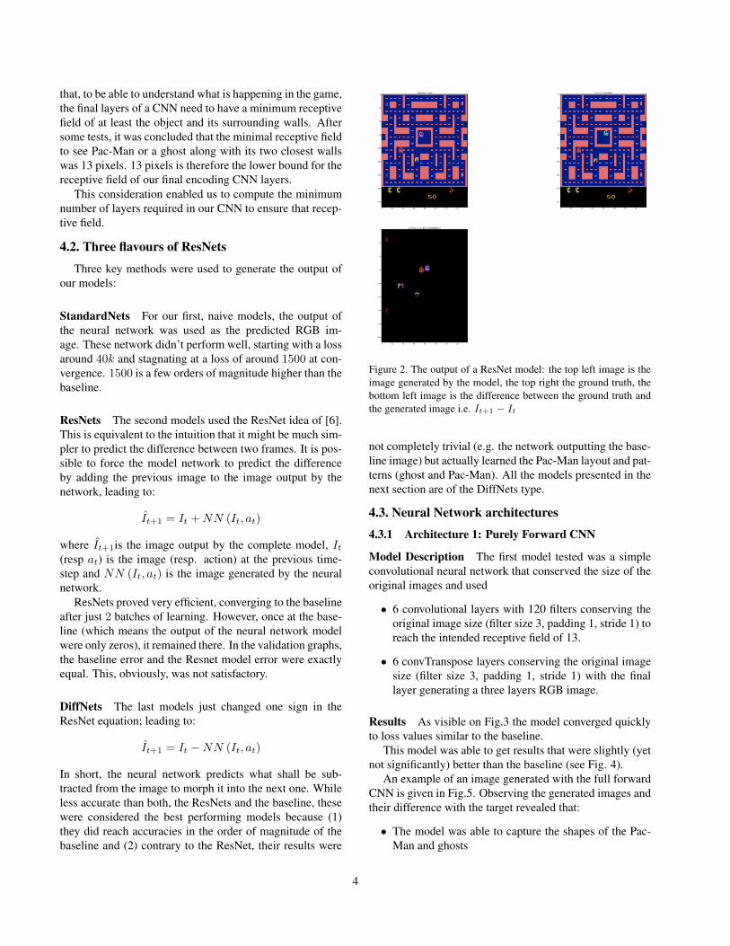
ResNets proved very efficient, converging to the baselineafter just 2 batches of learning. However, once at the base-line (which means the output of the neural network modelwere only zeros), it remained there. In the validation graphs,the baseline error and the Resnet model error were exactlyequal. This, obviously, was not satisfactory.
DiffNets The last models just changed one sign in theResNet equation; leading to:
It+1 = It −NN (It, at)
In short, the neural network predicts what shall be sub-tracted from the image to morph it into the next one. Whileless accurate than both, the ResNets and the baseline, thesewere considered the best performing models because (1)they did reach accuracies in the order of magnitude of thebaseline and (2) contrary to the ResNet, their results were
Figure 2. The output of a ResNet model: the top left image is theimage generated by the model, the top right the ground truth, thebottom left image is the difference between the ground truth andthe generated image i.e. It+1 − It
not completely trivial (e.g. the network outputting the base-line image) but actually learned the Pac-Man layout and pat-terns (ghost and Pac-Man). All the models presented in thenext section are of the DiffNets type.
4.3. Neural Network architectures
4.3.1 Architecture 1: Purely Forward CNN
Model Description The first model tested was a simpleconvolutional neural network that conserved the size of theoriginal images and used
• 6 convolutional layers with 120 filters conserving theoriginal image size (filter size 3, padding 1, stride 1) toreach the intended receptive field of 13.
• 6 convTranspose layers conserving the original imagesize (filter size 3, padding 1, stride 1) with the finallayer generating a three layers RGB image.
Results As visible on Fig.3 the model converged quicklyto loss values similar to the baseline.
This model was able to get results that were slightly (yetnot significantly) better than the baseline (see Fig. 4).
An example of an image generated with the full forwardCNN is given in Fig.5. Observing the generated images andtheir difference with the target revealed that:
• The model was able to capture the shapes of the Pac-Man and ghosts
4

Figure 3. Full loss history over a training run for the purely forwardCNN shows a healthy convergence.
Figure 4. Loss comparison between the baseline model and thepurely forward CNN.
• The RMSE criterion was pushing the model to meanvalues in areas of high uncertainty, resulting to moreblurry images around the Pac-Man, ghosts or blinkingobjects.
4.3.2 Architecture 2: Reducing Auto-Encoder
Model 1 had the shortcoming of having a lot of parame-ters. This not only made it slow to train and score but alsoprevented the use of RNNs as the output at the end of theencoder would be of far too high dimensionality.
Model 2 aimed to address this short-coming.
Model Description A CNN encoder divides the size ofthe image by 2 in the height and width, until a receptive
Figure 5. An image generated by the purely forward CNN. Thenetwork achieves lower loss by blurring the patterns of the Ghostsand Pac-Man
Figure 6. Reducing Convolutional Auto Encoder
Figure 7. CNN architecture to predict the next image
field of at least 13 is reached. To do this, two methods weretested: (1) using a stride of 2 and (2) using max-poolinglayers. A ConvTranspose decoder scales up the generatedfields until the size of the original image is recreated. Agraphical representation of the model is shown in Figures 6and 7
At each encoding layer, the number of channels was mul-tiplied by 2 until it reached a cap value, from which pointthe number of channels was kept constant. Vice-versa, the
5

Figure 8. Hyper-parameter tuning: setting the maximal number offilters right halves the loss. More filters is better, although thereis an inflection point around 400 filters from which the accuracyreturn for adding more filters (and hence parameters) strongly di-minishes.
number of channels in the decoder had hits number of chan-nels divided by two until it reached a cap. As discussed be-low, it turns out that the cap value on the maximum numberof channels for the encoder is a key hyper-parameter, centralto the performance of the model.
Hyper-parameters tuning Getting the reducing auto-encoder to top performance required selecting the correctparameters for dimensioning the network. The parametersof particular interest were:
• the number of layers in the network: smaller networkswith depth 6 for the encoder and decoder were foundto perform better.
• whether max pooling or striding was better for dimen-sionality reduction: both performed similarly.
• the maximum number of channels allowed in the en-coder: this was found to be the key hyper-parameter.Fig.8 illustrates the importance of that parameter.
• the learning routine (in our experience, Adam worksbest)
While many hyper-parameters were tried, only the plotsw.r.t to the maximum number of filters in the encoder isshown in the interest of space. This parameter was found tohave the greatest impact on loss.
Results The reducing AE achieved results similar to thepurely forward CNN, but with far fewer parameters.
Figure 9. Loss comparison between the baseline model and theReducing AE, here with a network having a cap at 1520 filters perlayer.
Figure 10. An image generated by a Reducing AE having a capat 1920 filters. The blurring effect on the Ghosts and Pac-Man iseven more pronounced
4.3.3 Architecture 3: Reducing Encoder encapsulatingan LSTM
Model Description Pac-Man follows the Markov prop-erty. Based on a suitable state st and the current image It,it is possible to fully determine the next state st+1 fromwhich one can generate the next image It+1. It is there-fore perfectly legitimate to try and use some RNNs as corecomponents of the architecture.
RNNs contain fully connected layers and are thereforevery memory intensive. This means that using them with-out triggering out of memory errors requires aggressivelyscaling down the original image of (3*210*160) to a muchsmaller parameters set.
6

Figure 11. Hyper-parameter tuning: setting the maximal numberof filters right halves the loss.
The architecture was therefore to:
1. Use a convolutional encoder to reduce the original im-age to a reasonable size.
2. Apply the RNN on the flattened output of that image.
3. Use a convolutional decoder to reconstruct the imagefrom the RNN updated state
Hyper parameters tuning Similar to the reducing auto-encoder, the LSTM model required tuning of its dimension-ing hyper-parameters. Note, that through the flatten opera-tion in this architecture, the LSTM hidden size and outputsize are direct linear combinations of the number of outputfilters in the encoder.
One new hyper-parameter was required in the RNN case:the number of steps the model would do back-propagationthrough time.
Similar to the reducing AE, the main hyper-parameterinfluencing the performance of the LSTM model was themaximum number of filters, or, equivalently, the size of theLSTM hidden state and cell. Figure 11 demonstrates theimpact of this parameter. Note that to prevent out of mem-ory exceptions, the size of the LSTM hidden state had to bekept small.
Results As shown in figure Fig.12 the LSTM model wasnot able to achieve a loss close to the baseline. A reason forthis is apparent in the analysis of Fig. 8: fitting the image inmemory required capping the number of filters used in theencoder to too low a number, resulting in a detrimental lossof information.
Figure 13 features an image generated with an LSTMmodel with hidden size 250. It shows that the LSTM model
Figure 12. Loss of a Convolutional Auto Encoder in an LSTMRNN compared to the baseline.
Figure 13. Image generated by a LSTM model with hidden size250
is struggling to even regenerate the Pac-Man board. One en-couraging note however is that, as visible on that image, theLSTM model seems to be able to decide whether the Pac-Man object will have an open mouth or not. This indicatesthat keeping a markovian state information indeed enabledthe model to (1) disambiguate between the open and closedPac-Man states and (2) start anticipating when these changeroughly occur.
5. Visualizing and interpreting output
Being able to interpret what is leading to errors is key indesigning a video prediction system. Fig.14 shows an ex-ample of the type of visualization that was developed forthat purpose. Each model’s accuracy was tested on gener-ated games of 500 frames, each of the model’s predictions
7

Figure 14. Example of the images used to get insight into a videoprediction model. The top left image is the generated image, thetop right the ground truth, the bottom left image is the differencebetween the generated image and the ground truth, the bottomright image is the difference between the ground truth and the pre-vious frame
was saved in a report pdf that enabled us to follow frame byframe what the model was doing.
This is how we determined, that the effect of biased sam-pling during the data generation process could lead to over-fitting (as presented in subsection 3.3). Examples of suchpdf reports can be found in the zip attached with the report.
6. ConclusionWe set out to solve the problem of video prediction ap-
plied to the Atari game called Pac-Man. We designed a fewmodels to try to evaluate ideas we learned from prior work.
We found that the performance of all our models wasvery close to that of the baseline with only a few modelsslightly outperforming it. It turned out to be a difficult taskto get the models to output images as sharp as those givenby the baseline.
We saw good performance with a purely forward CNNmodel. It was able to outperform the baseline model, how-ever the generated images were blurry mainly due to the factthat we used an RMSE loss.
The Reducing Auto-Encoder model was also able tobarely beat the baseline. The advantage it had over thepurely forward CNN model is that it used far fewer param-eters and generated sharper images.
The smaller parameter numbers of the Reducing Auto-Encoder model also allowed us to incorporate RNNs. Un-fortunately, even with the reduced parameter numbers, wedidn’t have sufficient hardware resources to run with thenumber of filters we needed. As such, the performance ofour RNN models was worse than that of the baseline. With
better hardware we believe we should have been able to getthe RNN models to beat our baseline.
7. Future WorkThere are a few ideas we would like to try next.
• Try feeding a sequence of images directly into ourCNN models, without resorting to RNNs. This takesless hardware resources and may give better results.
• Experiment with Gated Recurrent Units (GRUs).GRUs have been found to have similar performance toLSTM while having a much smaller parameter space.The fact that GRUs use less memory means it wouldbe possible to increase the number of filters at the endof the encoder, which, following the analysis of figureFig.8, is likely to improve generation.
• Train a separate model for each action taken by theplayer. This would result with 4x the number of pa-rameters but would likely slightly improve the perfor-mance.
• Given more time and hardware, expand the hyper-parameter tuning to more parameters. This would al-low us to better fine-tune the models.
• Experiment with different non-linearity functions totry to get the ResNet models to learn instead of out-putting 0s.
References[1] S. S. Beauchemin and J. L. Barron. The computation of op-
tical flow. ACM computing surveys (CSUR), 27(3):433–466,1995.
[2] G. Brockman, V. Cheung, L. Pettersson, J. Schneider,J. Schulman, J. Tang, and W. Zaremba. Openai gym, 2016.
[3] J. Chung, C. Gulcehre, K. Cho, and Y. Bengio. Empiricalevaluation of gated recurrent neural networks on sequencemodeling. CoRR, abs/1412.3555, 2014.
[4] B. J. Erickson, P. Korfiatis, Z. Akkus, T. Kline, andK. Philbrick. Toolkits and libraries for deep learning. Jour-nal of Digital Imaging, pages 1–6, 2017.
[5] I. Goodfellow, J. Pouget-Abadie, M. Mirza, B. Xu,D. Warde-Farley, S. Ozair, A. Courville, and Y. Bengio. Gen-erative adversarial nets. In Advances in neural informationprocessing systems, pages 2672–2680, 2014.
[6] K. He, X. Zhang, S. Ren, and J. Sun. Deep residual learn-ing for image recognition. In Proceedings of the IEEE Con-ference on Computer Vision and Pattern Recognition, pages770–778, 2016.
[7] S. Hochreiter and J. Schmidhuber. Long short-term memory.Neural computation, 9(8):1735–1780, 1997.
[8] M. Karl, M. Soelch, J. Bayer, and P. van der Smagt.Deep variational bayes filters: Unsupervised learningof state space models from raw data. arXiv preprintarXiv:1605.06432, 2016.
8
[9] D. Kingma and J. Ba. Adam: A method for stochastic opti-mization. arXiv preprint arXiv:1412.6980, 2014.
[10] D. P. Kingma and M. Welling. Auto-encoding variationalbayes. arXiv preprint arXiv:1312.6114, 2013.
[11] A. Krizhevsky, I. Sutskever, and G. E. Hinton. Imagenetclassification with deep convolutional neural networks. InAdvances in neural information processing systems, pages1097–1105, 2012.
[12] Y. LeCun, Y. Bengio, et al. Convolutional networks for im-ages, speech, and time series. The handbook of brain theoryand neural networks, 3361(10):1995, 1995.
[13] M. Mathieu, C. Couprie, and Y. LeCun. Deep multi-scalevideo prediction beyond mean square error. arXiv preprintarXiv:1511.05440, 2015.
[14] J. Oh, X. Guo, H. Lee, R. L. Lewis, and S. Singh. Action-conditional video prediction using deep networks in atarigames. In Advances in Neural Information Processing Sys-tems, pages 2863–2871, 2015.
[15] A. Radford, L. Metz, and S. Chintala. Unsupervised repre-sentation learning with deep convolutional generative adver-sarial networks. CoRR, abs/1511.06434, 2015.
[16] R. Villegas, J. Yang, S. Hong, X. Lin, and H. Lee. Decom-posing motion and content for natural video sequence pre-diction. ICLR, 1(2):7, 2017.
[17] P. Vincent, H. Larochelle, Y. Bengio, and P.-A. Manzagol.Extracting and composing robust features with denoising au-toencoders. In Proceedings of the 25th international confer-ence on Machine learning, pages 1096–1103. ACM, 2008.
9