Visual Pipe Mapping with a Fisheye Camera

Peter Hansen, Hatem Alismail, Peter Rander and Brett Browning

CMU-CS-QTR-116CMU-TR-RI-13-02

February 1, 2013

Robotics InstituteCarnegie Mellon University

Pittsburgh, Pennsylvania 15213

c© Carnegie Mellon University

This publication was made possible by NPRP grant #08-589-2-245 from the Qatar National Research Fund(a member of Qatar Foundation). The statements made herein are solely the responsibility of the authors.

Keywords:Robotics, computer vision, pipe inspection, LNG, 3D mapping, visual mapping, visual odometry, SLAM,

sparse bundle adjustment, structure from motion, fisheye.

Abstract

We present a vision-based mapping and localization system for operations in pipes such as those foundin Liquified Natural Gas (LNG) production. A forward facing, fisheye camera mounted on a prototype robotcollects imagery as it is tele-operated through a pipe network. The images are processed offline to estimatecamera pose and sparse scene structure where the results can be used to generate 3D renderings of the pipesurface. The method extends state of the art visual odometry and mapping for fisheye systems to incorporategeometric constraints based on prior knowledge of the pipe components into a Sparse Bundle Adjustmentframework. These constraints significantly reduce inaccuracies resulting from the limited spatial resolutionof the fisheye imagery, limited image texture, and visual aliasing. Preliminary results are presented for adataset collected in fiberglass pipe network which demonstrate the validity of the approach.

I

Contents

1 INTRODUCTION 1

2 FISHEYE CAMERA 1

3 VISUAL ODOMETRY AND MAPPING 23.1 Feature Tracking . . . . . . . . . . . . . . . . . . . . . . . . . . . . . . . . . . . . . . . . 33.2 Image classification: straight vs. T-intersection . . . . . . . . . . . . . . . . . . . . . . . . 33.3 Straight VO: Sliding Window SBA / local straight cylinder . . . . . . . . . . . . . . . . . . 53.4 T-intersections . . . . . . . . . . . . . . . . . . . . . . . . . . . . . . . . . . . . . . . . . . 5

4 EXPERIMENTS AND RESULTS 64.1 Visual Odometry . . . . . . . . . . . . . . . . . . . . . . . . . . . . . . . . . . . . . . . . 64.2 Dense Rendering . . . . . . . . . . . . . . . . . . . . . . . . . . . . . . . . . . . . . . . . 9

5 CONCLUSIONS 9

References 11

III

1 INTRODUCTION

Pipe inspection is a critical task to a number of industries, including Natural Gas production where pipesurface structure changes at the scale of millimeters are of concern. In this work, we report on the develop-ment of a fisheye visual odometry and mapping system for an in-pipe inspection robot (e.g. [11]) to producedetailed, millimeter resolution 3D surface structure and appearance maps. By registering maps over time,changes in structure and appearance can be identified, which are both cues for corrosion detection. More-over, these maps can be imported into rendering engines for effective visualization or measurement andanalysis.

In prior work [4], we developed a verged perspective stereo system capable of measuring accurate cam-era pose and producing dense sub-millimeter resolution maps. A limitation of the system was the inabilityof the camera to image the entire inner surface of the pipe. Here, we address this issue by using a forward-facing wide-angle fisheye camera mounted on a small robot platform, as shown in figure 1. This configu-ration enables the entire inner circumference to be imaged from which full coverage appearance maps canbe produced. Figure 1 also shows the constructed pipe network used in the experiments, and sample im-ages from the fisheye camera. The extreme lighting variations evident in the sample images pose significantchallenges during image processing, as discussed in section 3.

Our system builds from established visual odometry and multiple view techniques for central projectioncameras [8, 6, 12, 10, 9]. Binary thresholding, morphology and shape statistics are first used to classifystraight sections and T-intersection. Pose and structure results are obtained for each straight section using asliding window Sparse Bundle Adjustment (SBA) and localized straight cylinder fitting/regularization withinthe window. Fitting a new straight cylinder each window allows some degree of gradual pipe curvature to bemodeled, e.g. sag in the pipes. While more generalized pipe models may be more suited for this purpose, forexample cubic spline modeling of the pipe axis, computing the cylinder fitting regularization terms (distanceof scene points to cylinder) could be prohibitively expensive. After processing each straight section, resultsfor the T-intersections are obtained using SBA and a 2-cylinder intersection fitting/regularization – the 2cylinders are the appropriate straight sections of the pipe network. As a final step, the pose and structureestimates are used to produce a dense point cloud rendering of the interior surface of the pipe network.

Results are presented in section 4 which show the visual odometry, sparse scene reconstruction, and3D point cloud renderings for a one-loop dataset collected in our pipe network. These preliminary resultsillustrate the validity of the proposed system.

2 FISHEYE CAMERA

We use a 360◦ × 190◦ angle of view Fujinon fisheye lens fitted to a 1280pix × 960pix resolution CCDfirewire camera. Image formation is modeled using a central projection polynomial mapping. A scene pointXi projects to a coordinate η(θ, φ) = Xi/||Xi|| on the camera’s unit view sphere centered at the singleeffective viewpoint (0, 0, 0)T . The angles θ, φ are, respectively, colatitude and longitude. The projectedfisheye image coordinates are

u(u, v) =

[(k1θ + k2θ

3 + k3θ4 + k4θ

5) cosφ+ u0(k1θ + k2θ

3 + k3θ4 + k4θ

5) sinφ+ v0

], (1)

where u0(u0, v0) is the principal point. Multiple images of a checkerboard calibration target with knownEuclidean geometry were collected, and the model parameters fitted using a non-linear minimization of thesum of squared checkerboard grid point image reprojection errors.

1

Figure 1: The prototype robot retrofitted with a forward facing fisheye camera. Images are logged to the onboardcomputer as the robot traverses the 400mm (16 inch) internal diameter fiberglass pipe network. Samples images in astraight section and T-intersection are shown. All lighting was provided from 8 high intensity LEDs surrounding the

camera.

3 VISUAL ODOMETRY AND MAPPING

The visual odometry (VO) and mapping procedure is briefly summarized as follows:

A. Perform feature matching/tracking with keyframing.

B. Divide images into straight sections and T-intersections.

C. Obtain VO/structure estimates for each straight section using a sliding window SBA and localizedstraight cylinder fitting/regularization.

D. Obtain VO/structure estimates for each T-intersection using a 2 cylinder T-intersection model. This stepeffectively merges the appropriate straight sections.

2

The visual odometry steps (C and D) use different cylinder fitting constraints to obtain scene structureerrors included as a regularization error in SBA. As previously mentioned, we have observed this to be acritically important step which significantly improves the robustness and accuracy of the visual odometryand scene reconstruction estimates in the presence of1: limited spatial resolution from the fisheye camera;feature location noise due to limited image texture and extreme lighting variations; and an often high per-centage of feature tracking outliers due again to limited image texture and visual aliasing. At present anaverage a priori metric measurement of pipe radius r is used during cylinder fitting. Cylinder fitting with asupplied pipe radius also resolves monocular visual odometry scale ambiguity.

3.1 Feature Tracking

An efficient region-based Harris detector [5] based on the implementation in [10] is used to find a uniformfeature distribution in each image. The image is divided into 2 × 2 regions, and the strongest N = 200features per region are retained. Initial temporal correspondences are found using cosine similarity matchingof 11 × 11 grayscale template descriptors for each feature. Each of these 11 × 11 template descriptors isinterpolated from a 31 × 31 region surrounding the feature. Five-point relative pose [8] and RANSAC [3]are used to remove outliers and provide an initial estimate of the essential matrix E. We experimented withmultiple scale-invariant feature detectors/descriptors (e.g. SIFT [7], SURF [1]), but observed no significantimprovements in matching performance.

For all unmatched features in the first image, a guided Zero-mean Normalized Cross Correlation (ZNCC)is applied to find their pixel coordinate in the second image. Here, guided refers to a search within an epipo-lar region in the second image. Since we implement ZNCC in the original fisheye imagery, we back projecteach integer pixel coordinate to a spherical coordinate η, and constrain the epipolar search regions usingη2

T E η1 < thresh — the subscripts denote image 1 and 2. As a final step we implement image keyfram-ing, selecting only images separated by a minimum median sparse optical flow magnitude or minimumpercentage correspondences. Both minimums are selected empirically.

Figure 2 shows examples of the sparse optical flow vectors between keyframes in both a straight sectionand T-intersection. Features are ‘tracked’ across multiple frames by recursively matching using the methoddescribed.

3.2 Image classification: straight vs. T-intersection

To classify each image as belonging to a straight section or T-intersection, the image resolution is firstreduced by sub-sampling pixels from every second row and column. A binary thresholding is applied toextract dark blobs within the cameras field of view, followed by binary erosion and clustering of the blobs.The largest blob is selected and the the second moments of area L and Lp computed about the the blobcentroid and principal point, respectively. An image is classified as straight if the ratio Lp/L is less thanan empirical threshold; we expect to see a large round blob near the center of images in straight sections.Figures 3a through 3c show the blobs extracted in three sample images and the initial classification of eachimage. After initial classification, a temporal filtering is used to remove false positive classification, asillustrated in figure 3d. This filtering enforces a minimum straight/T-intersection cluster size.

1Fiberglass pipes are significantly more challenging to process than steel as they contain reduced image texture and exhibitgreater specular reflection. Steel pipes were unable to be used in the pipe network used for testing.

3

100

200

300

400

500

600

700

800

900

100

200

300

400

500

600

700

800

900

Figure 2: Sparse optical flow vectors in a straight section (left) and T-intersection (right) obtained using a combinationof Harris feature matching and epipolar guided ZNCC.

(a) Straight section (b) T-intersection (c) T-intersection

0 500 1000 1500 2000 2500

Non−straight

Straight

Keyframe Number

0 500 1000 1500 2000 2500

Non−straight

Straight

Keyframe Number

(d) Initial classification (top), and after applying temporal filtering (bottom). Each of the four T-intersection clusters isa unique T-intersection in the pipe network.

Figure 3: Straight section and T-intersection image classification. Example initial classifications (a-c), and the classifi-cation of all keyframes before and after temporal filtering (d).

4

3.3 Straight VO: Sliding Window SBA / local straight cylinder

For each new keyframe, the feature correspondences are used to estimate the new camera position andscene points. This includes using Nister’s 5-point algorithm to obtain an initial unit-magnitude pose changeestimate, optimal triangulation to reconstruct the scene points [6], and prior scene coordinates to resolverelative scale.

After every 50 keyframes, a modified sliding window SBA is implemented which includes a localizedstraight cylinder fitting used to compute a scene point regularization error. A 100 keyframe window sizeis used which, on average, equates to a segment of pipe approximately one meter in length. This SBA isa multi-objective least squares minimization of image reprojection errors εI and scene point errors εX. Anoptimal estimate of the camera poses P and scene points X in the window, as well as the fitted cylinder Care found which minimize the combined error ε:

ε = εI + εX. (2)

The image reprojection error εI is the sum of squared differences between all valid feature observations uand reprojected scene point coordinates u′:

εI =∑i

||ui − u′i||2, (3)

where u(u, v) and u′(u′, v′) are both inhomogeneous fisheye image coordinates.The scene point error term εX is a scalar weighted sum of squared errors between the optimized scene

point coordinates X and a fitted straight cylinder. The origin of the cylinder is the first camera pose Pm =[Rm|tm] in the sliding window, and is parameterized using 4 degrees of freedom:

C = [R | t]= [RX(γ)RY (β) | (tX , tY , 0)T ], (4)

where RA denotes a rotation about the axis A, and tA denotes a translation in the axis A. Each scene pointcoordinate Xi maps to a coordinate Xi in the cylinder coordinate frame using

Xi = R (RmXi + tm) + t. (5)

The regularization error εX is

εX = τ∑i

(√X2

i + Y 2i − r

)2

, (6)

where the pipe radius r is supplied. Adjusting the scalar τ controls the trade-off between the competingerror terms εI and εX. We use an empirically selected value τ = 100/r.

As noted previously, there are frequently many feature correspondence outliers resulting from the chal-lenging raw imagery. To minimize the influence of outliers, a Huber weighting is applied to individualerror terms before computing εI and εX. Outliers are also removed at multiple stages (iteration steps) usingMedian Absolute Deviation of the set of all signed Huber weighted errors u− u′.

3.4 T-intersections

The general procedure for processing the T-intersections is illustrated in figure 4. After processing eachstraight section, straight cylinders are fitted to the scene points in the first and last 1 meter segment (fig-ure 4a). In both cases, these cylinders are fitted with respect to the first and last camera poses as the origins,respectively, using the parameterization in (4).

5

As illustrated in fig. 4b, a T-intersection is modeled as two intersecting straight cylinders; the red cylinderintersects the blue cylinder at a unique point I. Let Pr be the first/last camera pose in a red section, and Cr

be the cylinder fitted with respect to this camera as the origin. Similarly, let Pb be the last/first camera posein a blue section, and Cb be the cylinder fitted with respect to this camera as the origin. The parameters ζrand ζb are rotations about the axis of the red and blue cylinders, and lr and lb are the signed distances ofthe cylinder origins O(Cr) and O(Cb) from the intersection point I. Finally, φ is the angle of intersectionbetween the two cylinder axes in the range 0◦ < φ < 180◦. These parameters fully define the change inpose Q between Pb and Pr, and ensure that the 2 cylinder axes intersect at a single unique point I. Letting

D = p([RZ(ζr)|(0, 0, lr)], [RZ(ζb)RY (φ)|(0, 0, lb)]T ]

), (7)

where p(b, a) is a projection a followed by b, and RA is a rotation about axis A, then

Q = p (inv(Cr), p(D,Cb)) , (8)

where inv(Cr) is the inverse projection of Cr.SBA is used to optimize all camera poses PT in the T-intersection between Pr and Pb, as well as all new

scene points X in the T-intersection, and the T-intersection model parameters Φ(ζr, lr, ζb, lb, φ). Again, theobjective function minimized is the same form as (2), which includes an image reprojection error (3) andscene fitting error (6). The same value τ = 100/r, robust cost function, and outlier removal scheme are alsoused.

Special care needs to be taken when computing the scene fitting error εX in (6) as there are two cylindersCr, Cb in the T-intersection model. Specifically, we need to assign each scene point to one of the cylinders,and compute the individual error terms in (6) with respect to this cylinder. This cylinder assignments isperformed by finding the distance to each of the cylinder surfaces, and selecting the cylinder for which theabsolute distance is a minimum. Figure 4c shows the results for one of the T-intersections after SBA hasconverged. The color-coding of the scene points (dots) represent their cylinder assignment.

4 EXPERIMENTS AND RESULTS

A single loop datasets was collected in our constructed 400mm (16 inch) internal diameter fiberglass pipenetwork. The total distance traversed during the rectangular shaped loop was approximately 34 meters. Therobot was tele-operating using images streamed over a wireless link, and all lighting was provided by 8 highintensity LEDs equipped on the robot — see figure 1. Over 24,000 grayscale images with 1280pix×960pixresolution were logged to the robot computer at 7.5 frames per second, from which 2760 keyframes wereautomatically selected. All image processing steps described in the previous section were implementedoffline.

4.1 Visual Odometry

The visual odometry and sparse scene reconstruction results for each of the straight sections was showpreviously in figure 4a. The complete results for the pipe network are provided in figure 5. The robots startand end locations are labeled, as well as the T-intersections T1 through T4. Note that no loop closure hasbeen used.

An ideal performance metric for our system is direct comparison of the visual odometry (camera pose)and scene structure results to accurate ground truth. However, obtaining suitable ground truth is particularlychallenging due to the unavailability of GPS in a pipe, and limited accuracy of standard grade InertialMeasurement Units (IMUs).

6

(a) Straight sections with cylinders fitted to endpoints.

(b) The two cylinder T-intersection model parameters(refer to text for detailed description). The red cylinderis constrained to intersect the blue cylinder at a uniquepoint I. Both pipes are assumed to have the same inter-

nal radius r.

(c) Visual odometry and scene reconstruction resultusing the T-intersection model. The scene pointshave been automatically assigned to each section al-lowing cylinder fit regularization terms to be used

within the SBA framework.

Figure 4: A T-intersection is modeled as the intersection of cylinders fitted to the straight sections of the pipe. Respec-tively, the blue and red colors distinguish the horizontal and vertical sections of the ‘T’, as illustrated in (b).

Our current ground truth is hand-held laser distance measurement estimates between all T-intersectioncentroids. For practical reasons, we used the center of the upper exterior surface of each T-intersectionas the centroid. These measurements are compared to the distances obtained from the visual odometry intable 1. For the visual odometry, each point of intersection I (see figure 4c) was used as the centroid.Unfortunately, there is no means for associating the laser and visual odometry reference points used for theT-intersection centroids, and as such the ground truth measurements contain some degree of uncertainty.The largest absolute error is between T4-T1, having a value of 0.051m (0.63%). This degree of accuracyis approaching the estimated uncertainty of the ground truth measurements. We are exploring alternatetechniques for obtaining more accurate ground truth.

7

(a) Visual odometry and sparse scene reconstruction: viewpoint 1.

(b) Visual odometry and sparse scene reconstruction: viewpoint 2.

(c) The pipe network with labeled T-intersections for reference.Observe that each of the long straight sections is constructed

from two straight segments of pipe.

Figure 5: Visual odometry (magenta line) and sparse scene reconstruction (black points) for the single loop pipe net-work dataset.

8

Distance T1-T2 T2-T3 T3-T4 T4-T1 T1-T3 T2-T4Laser (m) 8.150 8.174 8.159 8.110 11.468 11.493VO (m) 8.184 8.131 8.138 8.161 11.514 11.543

Error (m) 0.034 -0.043 -0.021 0.051 0.046 0.050Error (%) 0.42 -0.53 -0.26 0.63 0.41 0.44

Table 1: The T-intersection center-to-center distances obtain with a hand-held laser (ground truth), and visual odome-try – refer to figure 5. The signed error percentages are given with respect to the laser measurements.

In practice, modeling each long straight section of our pipe network as a perfect straight cylinder istoo restrictive. Firstly, each individual pipe segment contains some degree of curvature/sag. Secondly, theindividual segments used to construct the long straight sections of pipe (see figure 5c) are not preciselyaligned. It is for this reason that we only perform straight cylinder fitting locally as part of of the 100keyframe sliding window SBA. Doing so permits some gradual pipe curvature to be represented in theresults, as evident in 4c. However, for severe pipe misalignments or elbow joints, we expect the accuracy ofthe results to rapidly deteriorate. Some form of cubic spline modeling of the cylinder axis may be requiredin these scenarios, despite the significant increase in computational expense when computing the scene pointregularization errors. We aim to address these issues in future work.

A number of other directions for future work will be pursued to improve the accuracy and flexibility ofthe system. They include structured lighting options to estimate the internal pipe radius directly, and loopclosure detection/correction (e.g. [2]).

4.2 Dense Rendering

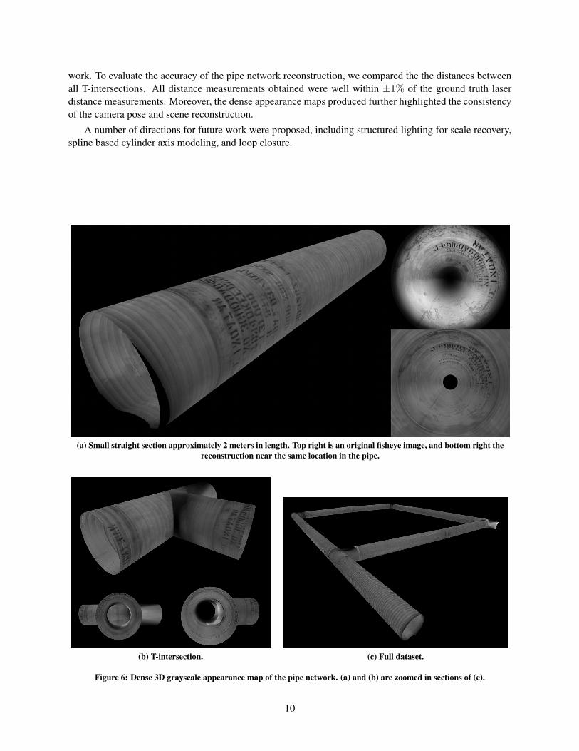
Using the visual odometry results, an appearance map of the pipe network was produced which may be usedas input for automated corrosion algorithms and direct visualization in rendering engines. Figure 6 showsthe appearance map of the pipe network, including and zoomed in view of a small straight section (figure 6a)and T-intersection (figure 6b) to highlight the detail. The consistency of the appearance, namely the letteringon the pipes, demonstrates accurate visual odometry estimates.

The appearance map produced is a dense 3D grayscale point cloud which could be extended to a fullfacet model. The Euclidean point cloud coordinates were set using the cylinder fitting results for both thestraight sections and T-intersections. The grayscale intensity value for each point was obtained by projectingthe point into all valid fisheye images and taking the average sampled image value. Here, valid is definedas having a projected angle of colatitude 45◦ < θ < 90◦ (i.e. near the periphery of the fisheye imagewhere spatial resolution is a maximum). A range of improvements are being developed to mitigate thestrong lighting variations in the rendered model. As evident in figure 6c, these are most prevalent in theT-intersections were the raw imagery can contain strong specular reflections and saturation.

5 CONCLUSIONS

An initial fisheye visual odometry and mapping system was presented for non-destructive automated corro-sion detection in LNG pipes. To improve the accuracy of the system, various cylinder fitting constraints forstraight sections and T-intersections were incorporated as regularization terms in sparse bundle adjustmentframeworks. The camera pose estimate and fitted cylinders are used as the basis for constructing dense piperenderings which may be used for direct visualization.

Results were presented for a single loop dataset logged in a 400mm internal diameter fiberglass pipe net-

9

work. To evaluate the accuracy of the pipe network reconstruction, we compared the the distances betweenall T-intersections. All distance measurements obtained were well within ±1% of the ground truth laserdistance measurements. Moreover, the dense appearance maps produced further highlighted the consistencyof the camera pose and scene reconstruction.

A number of directions for future work were proposed, including structured lighting for scale recovery,spline based cylinder axis modeling, and loop closure.

(a) Small straight section approximately 2 meters in length. Top right is an original fisheye image, and bottom right thereconstruction near the same location in the pipe.

(b) T-intersection. (c) Full dataset.

Figure 6: Dense 3D grayscale appearance map of the pipe network. (a) and (b) are zoomed in sections of (c).

10

References

[1] Herbert Bay, Andreas Ess, Tinne Tuytelaars, and Luc Van Gool. Speeded-up robust features (SURF). ComputerVision and Image Understanding, 110(3):346–359, June 2008.

[2] G Dubbelman, P Hansen, B Browning, and M. B Dias. Orientation only loop-closing with closed-form trajectorybending. In IEEE International Conference on Robotics and Automation, St. Paul, USA, May. 14-18 2012.

[3] Martin A Fischler and Robert C Bolles. Random sample consensus: A paradigm for model fitting with applica-tions to image analysis and automated cartography. Comms. of the ACM, pages 381–395, 1981.

[4] Peter Hansen, Hatem Alismail, Brett Browning, and Peter Rander. Stereo visual odometry for pipe mapping. InIROS, 2011.

[5] C.G. Harris and M.J. Stephens. A combined corner and edge detector. In Proceedings Fourth Alvey VisionConference, pages 147–151, 1988.

[6] Richard Hartley and Andrew Zisserman. Multiple View Geometry in Computer Vision. Cambridge Univ. Press,2003.

[7] David Lowe. Distinctive image features from scale-invariant keypoints. IJCV, 60(2):91–110, 2004.

[8] David Nister. An efficient solution to the five-point relative pose problem. PAMI, 26(6):756–770, June 2004.

[9] David Nister, Oleg Naroditsky, and James Bergen. Visual odometry. In Proceedings of the 2004 IEEE ComputerSociety Conference on Computer Vision and Pattern Recognition, 2004.

[10] David Nister, Oleg Naroditsky, and James Bergend. Visual odometry for ground vehicle applications. JFR,23(1):3–20, January 2006.

[11] Hagen Schempf. Visual and nde inspection of live gas mains using a robotic explorer. JFR, Winter, 2009.

[12] Bill Triggs, Philip F. McLauchlan, Richard I. Hartley, and Andrew W. Fitzgibbon. Bundle adjustment - a modernsynthesis. In Proceedings of the International Workshop on Vision Algorithms: Theory and Practice, ICCV ’99,pages 298–372, London, UK, 2000. Springer-Verlag.

11