Embed Size (px)
Citation preview

- 1 - 1
VISUAL AUGMENTATION FOR
VIRTUAL ENVIROMNENTS IN
SURGICAL TRAINING
Fani Deligianni
A dissertation submitted in partial fulfilment
of the requirements for the degree of
Doctor of Philosophy
of the
University of London
Department of Computing
Imperial College London 2006
- 2 - 2
ABSTRACT
Augmented reality is an important tool for surgical training and skills assessment. The use
of computer simulation, particularly the reliance on patient specific data for building
realistic models both in terms of biomechanical fidelity and photorealism has attracted
extensive interests in recent years. For example, by fusing real bronchoscopy video with 3D
tomographic data with the same patient, it is possible to generate photorealistic models that
allow high fidelity, patient specific bronchoscope simulation. In order to match video
bronchoscope images to the geometry extracted from 3D reconstructions of the bronchi,
however, robust registration techniques have to be developed. This is a challenging
problem as it implies 2D/3D registration with certain degrees of deformation and different
physiological responses.
In this thesis, we propose a new pq-space based 2D/3D registration method for camera pose
estimation in endoscope tracking. The proposed technique involves the extraction of
surface normals for each pixel of the video images by using a linear, local shape-from-
shading algorithm derived from the unique camera/lighting constrains of the endoscopes.
We demonstrate how to use the derived pq-space distribution to match to that of the 3D
tomographic model. The registration algorithm is further enhanced by introducing temporal
constrains based on particle filtering. For motion prediction, a second-order auto-regressive
model has been used to characterize camera motion in a bounded lumen as encountered in
bronchoscope examination. The proposed method provides a systematic learning procedure
with modular training from ground truth data such that information from different subjects
are integrated for creating a dynamic model, which accommodates the learnt behaviour.
To cater for airway deformation, an active shape model (ASM) driven 2D/3D registration
has been proposed. ASM captures the intrinsic variability of the tracheo-bronchial tree
during breathing and it is specific to the class of motion it represents. The method reduces
the number of parameters that control the deformation, and thus greatly simplifies the
optimisation procedure. Subsequently, pq-based registration is performed to recover both
the camera pose and parameters of the ASM. Radial Basis Functions (RBFs) are employed
to smoothly warp the 3D mesh based on the ASM point correspondences. The method also
exploits the recent development of five degrees-of-freedom miniaturised catheter tip
electromagnetic trackers such that the position and orientation of the bronchoscope can be
accurately determined under dis-occlusion and bleeding artefacts. The accuracy of the
proposed method has been assessed by using both a specially constructed airway phantom
with an electro-magnetic tracker, and in vivo patient data.

- 3 - 3
ACKNOWLEDGEMENTS
I would like to thank Professor Guang-Zhong Yang for giving me the opportunity to
accomplish this mission. I would also like to express my gratitude for his valuable
criticisms and ideas. In addition, I thank Dr. Adrian Chung for his contribution to my
research. I acknowledge that he kindly offered some of his beautiful illustrations (Figures:
2.1, 3.1, 6.1) to include in my thesis. I am also grateful to our clinical collaborators Dr.
Pallav Shah, Dr. Athol Wells and Dr. David Hansell. My funding came from EPSRC.
I thank Professor Nigel W. John and Dr. Anil Bharath for being my examiners.
I also appreciate the kind advices and support of Professor Daniel Rueckert for my further
development and career.
Sincere thanks to George Mylonas, Daniel Leff, Julian Leong, Benny Lo, Dr. Daniel
Stoyanov and Dr. Mohamed Elhelw for their enthusiasm and brain storming conversations.
Thanks also to Dr. Xia Peng Hu and Dr. Panos Parpas for their advices.
I would also like to thank all members of the VIP group. Both administrative and technical
staff in the department was always friendly and supportive. Particularly, I thank Surapa for
being my coffee mate and tolerating my murmur. Quian for her pleasant company. Su-Lin
for being helpful. Julien Nahed for his understanding. Louis for giving meaning to my
Greeks and being a cheerful fellow. Peter for his kindness. Karim for teaching me how to
play football. Marcus for our deep intellectual discussions. Kanwal for showing me how to
be independent. Dimitris for accounting me a strong opponent when playing sports.
I would also like to thank a number of other people that make my life in London beautiful.
Ah-Lai for our theatre trips. My Clayponds flatmates Nishani, Mariam and Laura for their
support and personal advices. George Tzalas, Alexandros, Marios and the rest basketball
fellows. Also I would like to thank my Lee Abbey friends for being such a pleasure to live
with: Justin, Kevin, Nam, Chris and Haidy, Stefania, Jey and so many more.
Nasoula, Kalu and Roulitsa remain always my best friends, though miles away.
To my parents, Christos and Eustratia, I express my deep love and gratitude. They deserve
much of the credits for giving me so much support and encouragement. I would also like to
commemorate my grandfather Parasxos and my grandmothers Maria and Fani.
Foremost, I would like to thank God for keeping me healthy and strong to continue. He
gives me the ability to exceed my limits.
Στους γονείς µου εκφράζω βαθειά αγάπη και ευγνωµοσύνη για τη διαρκή υποστήριξη
και υποµονή. Επίσης, θα ήθελα να µνηµονεύσω τον παππού µου Παράσχο και τις
γιαγιάδες µου Μαρία και Φανή.
Πάνω από όλα, ευχαριστώ το Θεό για τη δύναµη που µου δίνει να αγωνίζοµαι πέρα
από τα όρια µου.

- 4 - 4
To my family
Στους γονείς µου

- 5 - 5
CONTENTS ABSTRACT ........................................................................................................................................2
ACKNOWLEDGEMENTS ...............................................................................................................3
CONTENTS ........................................................................................................................................5
LIST OF FIGURES............................................................................................................................8
LIST OF TABLES............................................................................................................................12
LIST OF ABBREVIATIONS ..........................................................................................................13
CHAPTER 1 INTRODUCTION.....................................................................................................14
CHAPTER 2 SIMULATION IN MINIMALLY INVASIVE SURGERY...................................20
2.1 ELEMENTS IN MIS ....................................................................................................................21 2.2 SURGICAL EDUCATION AND SKILLS ASSESSMENT ....................................................................24
2.2.1 Traditional Surgical Education in MIS ............................................................................27 2.3 MEDICAL SIMULATORS AND VIRTUAL REALITY .......................................................................28
2.3.1 Current State-of-the-Art ...................................................................................................30 2.3.1.1 VR in Surgical Simulation....................................................................................................... 30 2.3.1.2 Augmented Reality in Surgical Simulation ............................................................................. 31
2.4 PATIENT SPECIFIC SIMULATION ................................................................................................32 2.4.1 Challenges in Surgical Simulation...................................................................................33
2.4.1.1 Photorealism – Visual Fidelity of Complex Structures............................................................ 33 2.4.1.2 Tissue Deformation and Biomechanical Modelling................................................................. 34 2.4.1.3 Physiological Response ........................................................................................................... 36 2.4.1.4 Haptics..................................................................................................................................... 37
2.5 SIMULATION IN BRONCHOSCOPY ..............................................................................................38 2.5.1 Airways Anatomy and Physiology....................................................................................38 2.5.2 Flexible Fibreoptic Bronchoscopy ...................................................................................41 2.5.3 Augmented Bronchoscopy ................................................................................................44 2.5.4 Technical Requirements of Augmented Bronchoscopy ....................................................45
2.5.4.1 High Resolution Image Acquisition of the Airways ................................................................ 46 2.5.4.2 Airway Tree Segmentation ...................................................................................................... 48 2.5.4.3 Volume and Surface Rendering............................................................................................... 49 2.5.4.4 Registration of the 3D Model with 2D Bronchoscope Video Sequences................................. 50 2.5.4.5 Navigation and Interactivity .................................................................................................... 51
2.6 DISCUSSION AND CONCLUSIONS ...............................................................................................52
CHAPTER 3 NON-RIGID 2D/3D IMAGE REGISTRATION....................................................54
3.1 IMAGE REGISTRATION IN MEDICAL IMAGING ...........................................................................55 3.2 2D/3D IMAGE REGISTRATION...................................................................................................56 3.3 MATHEMATICAL FORMULATION OF THE REGISTRATION PROBLEM ..........................................58 3.4 NON-RIGID 2D/3D REGISTRATION ...........................................................................................61
3.4.1 Transformation Models for Non-Rigid Registration ........................................................62 3.4.1.1 Spline Based Transformations ................................................................................................. 62 3.4.1.2 Free-Form Deformation........................................................................................................... 63 3.4.1.3 Physical Transformation Models ............................................................................................. 65
3.4.2 Surface Representation and Deformable Models.............................................................66 3.5 SIMILARITY MEASURES FOR IMAGE-BASED REGISTRATION .....................................................67
3.5.1 Intensity-Based Similarity Measures................................................................................68 3.5.1.1 Sum of Square Differences ...................................................................................................... 68 3.5.1.2 Normalised Cross-Correlation ................................................................................................. 69 3.5.1.3 Fourier Methods ...................................................................................................................... 69 3.5.1.4 Registration based on Geometrical Moment Invariants ........................................................... 70 3.5.1.5 Mutual Information.................................................................................................................. 70

- 6 - 6
3.5.1.6 Beyond Mutual Information .................................................................................................... 73 3.5.2 Feature-Based Techniques...............................................................................................76
3.5.2.1 Feature Detection..................................................................................................................... 76 3.5.2.2 Feature Correspondence and Pose Determination ................................................................... 77
3.6 OPTIMISATION TECHNIQUES .....................................................................................................80 3.7 EVALUATION OF 2D/3D REGISTRATION ALGORITHMS .............................................................80 3.8 DISCUSSION AND CONCLUSIONS ...............................................................................................81
CHAPTER 4 2D/3D REGISTRATION BASED ON PQ-BASED REPRESENTATION ..........83
4.1 PQ-BASED 2D/3D REGISTRATION .............................................................................................85 4.2 SHAPE-FROM-SHADING .............................................................................................................86
4.2.1 Human Vision and Depth Perception...............................................................................86 4.2.2 Understanding Image Intensities .....................................................................................87
4.2.2.1 Special Cases of Reflectance Map........................................................................................... 89 4.2.3 Image Formation..............................................................................................................91
4.3 SHAPE-FROM-SHADING IN BRONCHOSCOPY..............................................................................92 4.3.1 A closed-form solution for extracting pq-components .....................................................96 4.3.2 Extraction of pq-components from the 3D Model ..........................................................101 4.3.3 Similarity Measure .........................................................................................................101 4.3.4 Tissue Deformation ........................................................................................................105 4.3.5 Video Preprocessing ......................................................................................................106
4.4 EXPERIMENTS AND RESULTS ..................................................................................................107 4.4.1 Phantom Study ...............................................................................................................107 4.4.2 In vivo Validation...........................................................................................................109
4.5 RESULTS .................................................................................................................................110 4.5.1 Phantom study................................................................................................................110 4.5.2 In vivo validation............................................................................................................112
4.6 DISCUSSIONS AND CONCLUSIONS ...........................................................................................115
CHAPTER 5 INTEGRATION OF TEMPORAL INFORMATION.........................................117
5.1 A PROBABILISTIC FRAMEWORK IN VISUAL TRACKING ...........................................................120 5.2 ENDOSCOPE TRACKING BASED ON PARTICLE FILTERING .......................................................122 5.3 PREDICTION MODEL FOR THE BRONCHOSCOPIC CAMERA.......................................................124 5.4 LEARNING DYNAMICS OF BRONCHOSCOPE NAVIGATION .......................................................127
5.4.1 Modular Training...........................................................................................................129 5.4.2 Model Dynamic Variability............................................................................................132
5.5 EXPERIMENTAL DESIGN..........................................................................................................135 5.5.1 Obtaining the Training Sequences .................................................................................135
5.6 RESULTS .................................................................................................................................137 5.7 DISCUSSIONS AND CONCLUSIONS ...........................................................................................139
CHAPTER 6 EM TRACKERS IN BRONCHOSCOPE NAVIGATION..................................142
6.1 POSITIONAL TRACKERS IN MEDICAL APPLICATIONS ..............................................................143 6.2 MINIATURISED ELECTRO-MAGNETIC TRACKERS ....................................................................144
6.2.1 Accuracy Assessment and Metal Calibration of EM Trackers.......................................146 6.2.2 EM Tracking under Tissue Deformation and Patient Movements .................................149
6.3 EM TRACKING IN IMAGE-GUIDED BRONCHOSCOPY ...............................................................150 6.4 DECOUPLING OF GLOBAL AND RESPIRATORY MOTION...........................................................151
6.4.1 Principal Component Analysis.......................................................................................152 6.4.2 Wavelet Analysis ............................................................................................................153
6.5 EXPERIMENTAL DESIGN..........................................................................................................155 6.6 RESULTS .................................................................................................................................155 6.7 DISCUSSIONS AND CONCLUSIONS ...........................................................................................157
CHAPTER 7 NON-RIGID 2D/3D REGISTRATION WITH STATISTICAL SHAPE
MODELLING AND EM TRACKING.........................................................................................160
7.1 DEFORMABLE 2D/3D REGISTRATION .....................................................................................161 7.1.1 Deformation Modelling of the Airway Tree ...................................................................162 7.1.2 Active Shape Models ......................................................................................................163
7.1.2.1 Point Correspondence for the Active Shape Model ............................................................... 165 7.1.3 Mesh Warping with Radial Basis Functions ..................................................................167

- 7 - 7
7.1.4 A pq-based Similarity Measure ......................................................................................168 7.2 INCORPORATING EM TRACKING DEVICES ..............................................................................169 7.3 INCORPORATING TEMPORAL TRACKING .................................................................................170 7.4 EXPERIMENTAL DESIGN..........................................................................................................172
7.4.1 Video Preprocessing ......................................................................................................173 7.4.2 Phantom Setup ...............................................................................................................173 7.4.3 Ground Truth Data ........................................................................................................175
7.5 RESULTS .................................................................................................................................176 7.5.1 Assessment of Phantom Visual Reality...........................................................................176 7.5.2 Phantom Deformability ..................................................................................................177 7.5.3 Modelling of the Airways Respiratory Motion ...............................................................178 7.5.4 Accuracy of Deformable 2D/3D Registration ................................................................179 7.5.5 Temporal Tracking.........................................................................................................182
7.6 DISCUSSIONS AND CONCLUSIONS ...........................................................................................182
CHAPTER 8 CONCLUSIONS AND FUTURE WORK.............................................................186
8.1 MAIN CONTRIBUTIONS OF THE THESIS.....................................................................................187 8.1.1 A novel pq-space based registration scheme .................................................................187 8.1.2 Incorporation of temporal constrains based on particle filtering ..................................188 8.1.3 Miniaturised EM tracking and motion decoupling ........................................................188 8.1.4 Deformation modelling based on statistical shape models ............................................188
8.2 DISCUSSION AND CONCLUSIONS .............................................................................................189
APPENDIX A CONSTRUCTION OF THE PROJECTION MATRIX............................192
APPENDIX B KALMAN FILTERING ...............................................................................195
B.1 LIMITATIONS OF KALMAN FILTERING ....................................................................................197
BIBLIOGRAPHY...........................................................................................................................200

- 8 - 8
List of Figures
Figure 2.1: Main anatomy of the tracheobronchial tree.......................................................40 Figure 2.2: Augmented Reality combines Virtual Reality and Real Bronchoscope
Video to enhance the available information......................................................45 Figure 2.3: Technical requirements of augmented bronchoscopy.......................................46 Figure 3.1: Diagrammatic illustration of 2D/3D registration, before registration and
after registration. The contour overlay represents the projection of the 3D
model on the endoscopic frame before and after registration, respectively. ....57 Figure 3.2: The relationship between entropy and mutual information is depicted with
Venn diagrams....................................................................................................71 Figure 4.1: A schematic illustration of the basic configuration of the image formation
process for bronchoscope. In this figure, the camera coordinate system is
used with the Z-axis towards the image plane. N is the unit normal of a
surface point. Variables p, q are called the surface gradients at that point,
which are the slopes of the surface along the x and y direction,
respectively. In the case of endoscope images, the viewing vector (the
vector from the camera to the surface point) coincides with the lighting
vector (the vector from the light to the surface point). However, the
camera is close to the object and the angle between the viewing vector and
the optical axis, α , is not negligible..................................................................85 Figure 4.2: a) Some example endoscopic video frames. b) The derived pq-vectors
according to the linear shape-from-shading algorithm of Rashid et.al. c)
The depth map based on the integration of the pq-space. d-e) The
reconstructed surface is presented from two different angles. ........................100 Figure 4.3: a) A rendered pose of the 3D model and, b-c) the correspondent p, q
components are shown from left to right respectively. The p, q components
have been derived by differentiating the z-buffer. The colormap encodes
the value of p and q in each pixel. ...................................................................101 Figure 4.4: Examples demonstrating the effectiveness of the normalised weighting
factor. On the left column is the similarity measure with the normalised
weighting factor. On the right column is the similarity measure based on
the angle. The position at (0,0) coordinates corresponds to the optimal pose
based on visual inspection and manual refinement. By evaluating the
similarity measure in a square area around this pose, the shape of the
function to be optimised is revealed. The white square indicates where the
minimum lie. ....................................................................................................104 Figure 4.5: a) A video frame from a deformed airway phantom, b) the associated p-q
space deformation map where bright intensity signifies the amount of
deformation detected. (c-d) The superimposed 3D rendered image with
pose estimated from intensity-adjusted registration and pq space
registration with deformation weightings, respectively. .................................105 Figure 4.6: The pre-processing steps applied to the bronchoscope videos before 2D/3D
registration. a) Original video frame acquired from the prototype
bronchoscope, b) de-interlaced video frame, c) after lens distortion
correction, and d) final smoothed image by using an anisotropic filter that
preserves local geometrical features. ...............................................................106 Figure 4.7: a) An airway phantom made of silicon rubber and painted with acrylics
was constructed in order to assess the accuracy of the pq-based
registration. b) A real-time six DOF EM tracker motion tracker
- 9 - 9
(FASTRAK, Polhemus) was used to validate the 3D camera position and
orientation.........................................................................................................108 Figure 4.8: Assessment of manual alignment error compared to the EM tracker as
assessed by using the 3D bronchial model. a) Euclidean distance between
the first and subsequent camera positions as measured by the EM tracker
and after manual alignment with step equal to 10. b) Inter-frame angular
difference between manual alignment and readings from the EM tracker.....109 Figure 4.9: Euclidean distance between the first and subsequent camera positions as
measured by four different tracking techniques corresponding to the
conventional intensity based 2D/3D registration with or without manual
lighting adjustment, the EM tracker and the proposed pq space registration
technique...........................................................................................................111 Figure 4.10: Inter-frame angular difference at different time of the video sequence, as
measured by the four techniques described in the above figure. ....................111 Figure 4.11: In vivo validation results for a patient study. The left column shows
examples of real bronchoscopic images. The right column presents the
virtual bronchoscopic images after pq-space based 2D/3D registration.........112 Figure 4.12: In vivo validation: Euclidean distance between the first and subsequent
camera positions as measured by the pq-based 2D/3D registration and
from manual alignment for ten random frames of the sequence. ...................114 Figure 4.13: In vivo validation: Inter-frame angular difference at different time of the
video sequence, as measured by the two techniques described in Figure
4.12. ..................................................................................................................114 Figure 4.14: Common image artefact that can affect image-based 2D/3D registration
techniques: a) excessive bleeding due to pathology, b) appearance of
bubbles when patient coughs, and c-d) large tissue deformation between
successive image frames. .................................................................................114 Figure 5.1: These frames demonstrate local ambiguities during endoscope navigation
due to the relatively symmetrical branching structure of the
tracheobronchial tree. For example, frames a) and c) are branches that
show the left and right bronchus after passing the main bifurcation, frame
b). However, it is difficult to locate the position of the camera by
inspecting individual frames. ...........................................................................119 Figure 5.2: A schematic diagram of the proposed framework. .........................................121 Figure 5.3: a-b) Training results based on a first order ARG model. c-d) Training
results based on a second order Autoregressive Model. .................................127 Figure 5.4: (a,c,e) Training results based on a 6DoF, second order Autoregressive
Model. (b,d,f) Training results based on two simultaneously second order
Autoregressive Models of tracking the position and the orientation of the
camera separately. ............................................................................................130 Figure 5.5: Four sequences of the camera position during in vivo navigation have been
used for modular training. These have been extracted from four different
subjects. This figure presents the Euclidean distance from an initial
reference point of each of these training sequences. .......................................132 Figure 5.6: Assessment of the accuracy of the training model and the effect of
excluding a), and including b), mean value estimation of X as part of the
state vector........................................................................................................134 Figure 5.7: The effect of the interpolation on the dynamics of the prediction model.
(a,c) correspond to B-spline interpolation and (b,d) correspond to
Piecewise Hermite interpolation......................................................................137 Figure 5.8: Bar chart showing the quantitative assessment of the pq-space based
registration with and without the condensation algorithm..............................138

- 10 - 10
Figure 5.9: The effect of airway deformation and partial occlusion of the image due to
mucosa and blood on the accuracy of the 2D/3D registration technique
without (mid-column) and with (right-column) predictive camera tracking..141 Figure 6.1: A diagrammatic illustration of the EM tracking sensor setup, where one
catheter tip sensor is inserted into the patient’s lungs and another is
attached on the chest of the patient to monitor global and respiratory
motion...............................................................................................................151 Figure 6.2: Wavelet analysis: X, Y and Z positional data has been acquired from an
EM tracker attached on the skin of a healthy subject in order to assess the
wavelet technique of filtering sudden movements similar to those that are
introduced in a bronchoscopy session when the patient coughs. We used
Daubechies (db10) mother wavelets to analyze the signals............................154 Figure 6.3: The energy function after analyzing the X-motion signal. Similar results
have been acquired from analyzing either the Y or the Z component. ...........156 Figure 6.4: Example position traces sampled by the EM tracker and the extracted
respiratory motion pattern................................................................................157 Figure 7.1: A schematic illustration of the proposed non-rigid 2D/3D registration
framework with 5 DoF EM tracking and ASM for deformation modelling. .162 Figure 7.2: a) The extracted geometrical centroids of each airway branch of each CT
slice (red dots) are shown for six 3D airway meshes that correspond to six
phases of respiration of the phantom model. The blue line represents the
extracted skeletons and the bifurcation and terminal points are marked
with yellow star-dot markers. The green line shows the correspondence
between the extracted points. b) For each of the skeleton points, the
surface perpendicular to the skeleton axis was subsequently defined and its
intersection with the 3D mesh was estimated. For simplicity, four surface
control points corresponding to each skeleton landmark were used. .............166 Figure 7.3: The bronchoscope navigation paths involved in this study, where the
camera travels from the right branch (frame-9780) to the trachea (frame-
10845) and then continues to the left branch (frame-12501)..........................172 Figure 7.4: Illustrations of the phantom setup during two different deformation stages.
a) The maximum level of deformation is achieved when the balloon is
relatively full of air, and b) shows the resting state when the balloon is
empty. ...............................................................................................................174 Figure 7.5: Example bronchoscope video frames acquired during the phantom
experiment where the images have been pre-processed to alleviate the
effect of de-interlacing and lens distortion. .....................................................176 Figure 7.6: The normalised mesh displacement between successive deformation stages
of the phantom..................................................................................................177 Figure 7.7: The result of applying the ASM to the reconstructed 3D volumes,
illustrating the warped 3D mesh by using the RBF along the first principal
mode of the shape variation. The red, green, and blue meshes correspond
to varying 13 λ− , 0, and 13 λ+ from the mean shape. ............................178
Figure 7.8: The performance of the proposed registration algorithm by using the EM
tracking data combined with the deformable model as determined by
ASM. Left-column: the bronchoscope view of the phantom airway; Mid-
column: the corresponding view of the 3D model determined by the 5 DoF
catheter tip EM tracker where significant mis-registration is evident due to
unknown rotation and airway deformation; Right-column: the result of
applying the proposed registration algorithm demonstrating the visual
accuracy of the method. ...................................................................................180 Figure 7.9: The recovered deformation as projected onto the first principal axis of the
ASM model where the corresponding ground truth value (dotted curve) as

- 11 - 11
determined by the 6 DoF EM tracker from Equation (7.21) is provided for
comparison. ......................................................................................................181 Figure 7.10: Bland-Altman plot of the non-rigid registration results as compared to the
ground truth. .....................................................................................................181 Figure 7.11: Euclidean distance between the first and subsequent camera position as it
has been predicted from the Condensation algorithm with relation to the
EM tracking data. .............................................................................................182 Figure A.1: In OpenGL, coordinates are flipped around the horizontal axis. ....................193

- 12 - 12
List of Tables
Table 3.1: Common geometric transformations. a) Original Shape, b) Rigid
transformation can be expressed with two components: a rotation R and a
translation t. c) Affine transformation preserves parallel lines but A is not
an orthogonal matrix. d) The projective part is expressed as a three
dimensional vector vT. ........................................................................................60
Table 5.1: Quantitative assessment of the pq-space based registration with and
without the Condensation algorithm (pq-CD), respectively...........................137 Table 6.1: Correlation of the waveform estimated by the suggested respiratory
decoupling motion technique with the waveform estimated by relative
position of two sensors.....................................................................................156 Table 7.1: Modelling error associated with omitting each eigenvalue individually........179

- 13 - 13
List of Abbreviations
AR
ARG
ASM
BRDF
Condensation
CT
DoF
EM
FEM
FFB
FFD
HAMMER
HU
IBMR
ICP
LUS
MI
MIS
MR
MRI
NCC
NMI
NURBS
PCA
PDM
POSIT
RSRM
SFS
SSD
VB
VR
Augmented Reality
AutoRegressive
Active Shape Models
Bidirectional Reflectance Distribution Function
Conditional Density Propagation
Computed Tomography
Degree of Freedom
ElectroMagnetic
Finite Element Models
Flexible Fibreoptic Bronchoscopy
Free-Form Deformation
Hierarchical Attribute Matching Mechanism
Hounsfield Units
Image Based Modelling and Rendering
Iterative Closest Point
Laparoscopic Ultrasonography
Mutual Information
Minimally Invasive Surgery
Magnetic Resonance
Magnetic Resonance Imaging
Normalised Cross-Correlation
Normalised Mutual Information
Non-Uniform Rational B-Splines
Principal Component Analysis
Point Distribution Model
Pose from Orthography and Scaling with Iterations
Rotational Symmetric Reflectance Map
Shape From Shading
Sum of Square Distances
Virtual Bronchoscopy
Virtual Reality
- 14 - 14
Chapter 1
Introduction
ver the last ten years, there have been major advances in Minimally Invasive Surgery
(MIS). Bronchoscopy and laparoscopy are two common procedures in MIS, which
are carried out through natural body openings or small artificial incisions. With these
techniques, diagnostic accuracy and therapeutic success are improved when compared to
conventional techniques, while at the same time patient trauma and the duration of
hospitalisation are greatly reduced. With the maturity of MIS in recent years, there has been
an increasing demand of patient specific simulation devices for both training and skills
assessment. This is due to the fact that the complexity of the instrument controls, restricted
vision and mobility, difficult hand-eye co-ordination, and a lack of tactile perception are
major obstacles in performing MIS. They require a high degree of manual dexterity and
hand-eye coordination from the operator. Flexible fibre-optic bronchoscopy, for example, is
normally performed on patients who are fully awake or with light conscious sedation. The
procedure can entail considerable discomfort if it is not handled properly. Training
according to the traditional apprenticeship scheme is useful but can result in prolonged
surgical procedures with increased patient discomfort and a potential risk of further
complications. Simulation devices provide an attractive alternative that offers a number of
advantages in terms of cost, time and efficiency.
The use of computer simulation has attracted extensive interests in recent years. For most
of the current simulation systems, however, the degree of visual realism is severely limited.
In endoscope simulations, most systems have used standard polygon rendering techniques
with synthetic texture mapping. Texture mapping is usually uniform throughout the whole
simulation, and even in cases where special visual effects, such as polyps or inflammation,
are provided, they are limited in both accuracy and adaptability. Natural objects, such as the
colon or the bronchi show considerable diversity of shape and texture. The problem of
generating realistic structure and surface properties has hindered the production of generic
O

- 15 - 15
test-case databases. These drawbacks highlight the importance of augmenting virtual
endoscopic views with patient specific endoscopic videos.
In this thesis, we aim to rely on patient specific data for building anatomical models of MIS
both in terms of biomechanical fidelity and photorealism. In Chapter 2, the problem and
major challenges of MIS simulation are discussed. Particular attention is directed to
bronchoscope simulation, which is used as an exemplar to highlight the visual, physical,
and tactile realities required for MIS simulation. The objective of this chapter is to establish
the basic requirements for creating photorealistic bronchoscopy simulation and identify the
drawbacks of existing approaches.
One of the key computational issues identified in Chapter 2 for bronchoscopy simulation is
how to fuse real-bronchoscopy video with 3D tomographic data of the same patient. In
order to match video bronchoscope images to the geometry extracted from 3D
reconstructions of the bronchi, robust registration techniques have to be developed. This is
a challenging problem as it implies 2D/3D registration with the presence of local
deformation. In Chapter 3, existing methods for 2D/3D registration based on intensity and
geometric features are reviewed. Both techniques involve optimising a similarity measure
that evaluates how close a 3D model viewed from a given camera pose is to the current 2D
video frame. Intensity based techniques entail comparing a predicted image of the object
with the 2D image without any structural analysis. With this approach, similarity measures
such as cross-correlation and mutual information are typically used. Mutual information
exploits the statistical dependency of two datasets and is particularly suitable for multi-
modal images. Existing methods, however, are based on special illumination conditions that
may not match bronchoscope images because they are illuminated by a light source that is
close to the tissue surface and are heavily affected by inter-reflections. In this case, the
intensity decreases with the square of the distance from the light source and it is essential to
adjust the illumination conditions of the rendered 3D model in order for the intensity-based
techniques to work. The method is further complicated by specular reflections due to the
mucous layer of the tissue surface, which is difficult to model for simulated views. As an
alternative, feature based techniques depend on the alignment of corresponding image
features, which are relatively robust against changes in lighting conditions. However, using
features purely based on visual appearance is not reliable due to the richness of surface
texture observed in bronchoscope views, which are absent in 3D tomographic images.
The basic hypothesis of the thesis is that a robust 2D/3D registration can be achieved by
exploiting the unique geometrical constraint between the camera and the light source in
bronchoscopic procedures. Shape-from-shading techniques utilise this information to

- 16 - 16
recover surface structure that can be described by ( ),p q vectors. This approach directly
relates the intensity information available in endoscopic image frames to the 3D CT data.
Based on this hypothesis, a novel pq-space based 2D/3D registration technique is
developed. In the specific case of using perspective projection with a point light source near
the camera, the use of intensity gradient can reduce the conventional shape-from-shading
equations to a linear form, which suggests a local shape-from-shading algorithm that avoids
the complication of changing surface albedos. Albedo is a unitless measure indicative of the
surface’s reflectivity. We have demonstrated in this chapter how to effectively use the
derived pq-space distribution to match to that of the 3D tomographic model. The validation
of the accuracy of the method is based on the positional and angular errors by using 6 DoF
Electro-Magnetic (EM) tracking as the reference. The major advantage of the proposed pq-
space based method is that it depends neither on the illumination of the 3D model, nor on
feature extraction and matching. Furthermore, the temporal variation of the pq distribution
permits the identification of localized deformation, which offers a means of excluding these
areas from the registration process.
Since 2D bronchoscope video only provides a localised view of the inner surface of the
lumen, the exact 3D location of the structure it represents is ambiguous. Different segments
of the airways may well have a similar local structure. Therefore, the use of temporal
information to derive the trajectory of the bronchoscope camera in 3D space is important
for resolving such ambiguities. Another advantage of using temporal correspondence is that
the estimates of the camera’s orientation and position can be used to accelerate the
registration process. In previous research, Kalman filtering has been used but it is generally
restricted to situations where the probability distribution of the state variables is unimodal.
In bronchoscopy, tissue deformation, inter-reflection, and view dependent specularity due
to mucosa can influence the accuracy of registration algorithms, and the resultant
probability density function of the state vector can be multi-modal. In Chapter 5, a
predictive tracking algorithm based on the Condensation algorithm has been developed.
The method is designed to cater for the general situation when several competing
observations form a non-Gaussian state-density. It uses a stochastic approach that has very
few restrictions on the system/measurement models used and the distribution of error
sources. An autoregressive algorithm is used as a predictive model, which is based on the
fact that during bronchoscope navigation, the motion is restricted to a bounded area and a
rapidly moving camera is more likely to slow down or change direction, rather than
accelerate further. The method provides a systematic learning procedure with modular
training from the ground truth data such that information from different subjects are
integrated for creating a dynamical model that can accommodate the learnt behaviour.

- 17 - 17
The results presented in Chapters 4 and 5 show that the proposed pq-space based 2D/3D
registration combined with temporal tracking are effective, but they can be problematic
when large airway deformation is encountered. This, however, is common in practical
examinations due to extreme breathing and deformation (such as coughing) of the patient.
With the recent advances of miniaturised EM tracking devices, it is now possible to insert
these devices into the biopsy channel of the bronchoscope to provide in situ measurement
of the camera pose of the bronchoscope. In Chapter 6, issues related to the practical use of
the EM tracker are discussed. Since airways are highly deformable and their shape is
affected by respiratory motion, the use of the EM tracking data must first consider the
alignment of the fixed EM coordinates with the moving frame-of-reference of the
bronchoscope camera. In this chapter, both respiration and patient movements are
considered, and a global and local respiratory motion decoupling technique is proposed.
After global and local frame-of-reference alignment, the positional and orientation data
derived from the EM tracker can be used for 2D/3D registration. This significantly
enhances the robustness of the technique as temporal tracking is now more immune to
discontinuities caused by abrupt airway motions. This provides the scope in exploiting the
improved accuracy to examine detailed local deformation of the airways. To address the
high degrees-of-freedom involved in bronchial deformation during the 2D/3D registration
process, an active shape model has been developed in Chapter 7 to capture the principal
modes of airway deformation during respiration such that the registration process can be
implemented with a much reduced parameter space to allow for simultaneous registration
and deformation tracking.
Finally, limitations of the current technique and possible improvements of the proposed
registration framework are discussed in Chapter 8. To our knowledge, this is the first
systematic study of 2D/3D registration incorporating airway deformation with
comprehensive phantom and patient data validation. The work presented in this thesis has
been included in a number of peer-reviewed academic journals and conference proceedings.
1. Deligianni F, Chung A, Yang GZ. Non-Rigid 2D/3D Registration for Patient Specific
Bronchoscopy Simulation with Statistical Shape Modelling. IEEE Transactions on
Medical Imaging, 2006; 25(11): 1462-1471.
2. Deligianni F, Chung A, Yang GZ. Patient-Specific Bronchoscope Simulation with
pq-Space-Based 2D/3D Registration. Computer Aided Surgery 2004; 9(5):215-226.
3. Deligianni F, Chung A, Yang G-Z. Non-Rigid 2D-3D Registration with Catheter Tip
Em Tracking for Patient Specific Bronchoscope Simulation. In: Proceedings of
- 18 - 18
Medical Image Computing and Computer Assisted Intervention (MICCAI06),
Copenhagen, Denmark, 2006.
4. Deligianni F, Chung A, Yang GZ. Predictive Camera Tracking for Bronchoscope
Simulation with Condensation. In: Proceedings of International Conference on
Medical Image Computing and Computer Assisted Intervention (MICCAI05), Palm
Springs, California, USA, 2005; 910-916.
5. Deligianni F, Chung A, Yang GZ. Decoupling of Respiratory Motion with Wavelet
and Principal Component Analysis. In: Proceedings of Medical Image Understanding
and Analysis (MIUA04), London, UK, 2004; 13-16.
6. Deligianni F, Chung A, Yang GZ. 2D/3D Registration Using Shape-from-shading
Information in Application to Endoscope. In: Proceedings of Medical Image
Understanding and Analysis (MIUA03), Sheffield, UK, 2003; 33-36.
7. Deligianni F, Chung A, Yang GZ. pq-Space Based 2D/3D Registration for
Endoscope Tracking. In: Proceedings of Medical Image Computing and Computer
Assisted Intervention (MICCAI03), Montréal, Québec, Canada, 2003; 311-318.
Collaboration with other colleagues of the group has also led to joint publications that are
related to the project. They include:
1. Chung AJ, Deligianni F, Shah P, Wells A, Yang GZ. Patient Specific Bronchoscopy
Visualisation through BRDF Estimation and Disocclusion Correction. IEEE
Transactions of Medical Imaging 2006; 25(4):503- 513.
2. Chung AJ, Deligianni F, Hu XP, Yang GZ. Extraction of Visual Features with Eye
Tracking for Saliency Driven 2D/3D Registration. Image and Vision Computing
2005; 23:999-1008.
3. Stoyanov D, Mylonas GP, Deligianni F, Darzi A, Yang GZ. Soft-Tissue Motion
Tracking and Structure Estimation for Robotic Assisted Mis Procedures. In:
Proceedings of 8th International Conference on Medical Image Computing and
Computer Assisted Intervention (MICCAI05), Palm Springs, California, USA, 2005;
139–146.
4. Mylonas GP, Stoyanov D, Deligianni F, Darzi A, Yang GZ. Gaze-Contingent Soft
Tissue Deformation Tracking for Minimally Invasive Robotic Surgery. In:
Proceedings of 8th International Conference on Medical Image Computing and
Computer Assisted Intervention (MICCAI05), Palm Springs, California, USA, 2005;

- 19 - 19
843–850.
5. Chung AJ, Deligianni F, Shah P, Wells A, Yang GZ. Vis-a-Ve: Visual Augmentation
for Virtual Environments in Surgical Training. In: Proceedings of Eurographics /
IEEE VGTC Symposium on Visualization, Leeds, UK, 2005; 101-108.
6. Chung A, Deligianni F, Elhelw M, Shah P, Wells A, Yang GZ. Assessing Realism of
Virtual Bronchoscopy Images via Specialist Survey and Eye-Tracking. In:
Proceedings of Medical Image Perception Conference XI (MIPS XI), Abstract,
Windermere, UK, 2005.
7. Chung AJ, Edwards PJ, Deligianni F, Yang GZ. Freehand Cocalibration of an
Optical and Electromagnetic Tracker for Navigated Bronchoscopy. In: Proceedings
of Medical Imaging and Augmented Reality (MIAR 2004), Beijing, China, 2004;
320-328.
8. Chung AJ, Deligianni F, Shah P, Wells A, Yang GZ. Enhancement of Visual Realism
with BRDF for Patient Specific Bronchoscopy Simulation. In: Proceedings of
Medical Image Computing and Computer Assisted Intervention (MICCAI04),
Rennes, France, 2004; 486-493.
9. Chung AJ, Deligianni F, Hu XP, Yang GZ. Visual Feature Extraction Via Eye
Tracking for Saliency Driven 2D/3D Registration. In: Proceedings of Eye Tracking
Research and Applications (ETRA04), San Antonio, Texas, USA, 2004; 49-54.

- 20 - 20
Chapter 2
Simulation in Minimally Invasive
Surgery
inimally Invasive Surgery (MIS), also known as minimal access surgery, refers to
surgical operations that are carried out through natural body openings or small
surgical incisions. Bronchoscopy and laparoscopy are two examples of MIS. The first
laparoscopic cholecystectomy was performed in 1987 by Dr Phillipe Mouret and it is
widely accepted that MIS is the most significant change in surgical practice since the
introduction of aseptic technique and safe anaesthesia [1, 2].
MIS has become possible through a combination of several technological advances in
optics, illumination systems, insufflation devices, and imaging techniques. In 1954, Harold
Hopkins, published in Nature an article reporting the transmission of images along tiny
glass fibers and produced the first fibre-scope image. Five years later, he described a
method that could efficiently transmit light through a solid quartz rod without introducing
heat [3]. The Hopkins rod lens system and the subsequent miniaturisation of video cameras
have allowed surgeons to visualise inside the body with clarity that is comparable to that of
open surgery. In the early 1970s, flexible endoscope found widespread applications in
surgery. At the same time, insufflation devices have also been developed to allow
controlled distension of body cavities with CO2 gas to provide surgeons with improved
work-space.
With MIS, improvements in diagnostic accuracy and therapeutic outcome are significant
when compared to conventional techniques. Firstly, small incisions lead to less post-
operative pain and a reduction in the morbidity due to immobility. Secondly, patient trauma
M
- 21 - 21
and the duration of hospitalisation are greatly reduced. Thirdly, the small port-holes of MIS
surgery lead to improved cosmetic results. There are also a number of other advantages of
MIS, which include improved visualisation of inaccessible areas, minimisation of the risk
of adhesive intestinal obstruction, and a decreased inflammatory response.
However, MIS can also cause a number of complications if it is not handled properly. The
creation of a gas filled cavity, as well as the prolongation of the operation can carry certain
risks [4, 5]. It can also cause significant mental and physical stress to the surgeon by
standing in a fixed position for long hours. Most importantly, advanced surgical skills and
manual dexterity are required for MIS and they are often associated with a steep ‘learning
curve’ [6]. Complications usually occur early in the surgeon’s overall experience of MIS,
or when an experienced surgeon is expanding into new procedures.
MIS requires a range of skills that are different from those used in open surgery. This is due
to the fact that the complexity of the instrument control, restricted vision and mobility,
difficulty in hand-eye co-ordination, and the lack of tactile perception are major obstacles
in performing MIS. In MIS, the view of the operative field is displayed on a 2D monitor
that is widely separated from the field of action. The two-dimensional view of a three-
dimensional field has to be interpreted and synchronized with instrument movement. Depth
information has to be extracted from 2D image cues in order to be able to navigate inside
the cavity. In laparoscopy, the surgeon also has to adapt to the fulcrum effect, whereby the
tip of the instrument moves in a direction that is opposite to the surgeon’s hand around the
port. The fulcrum effect causes a fundamental visual-alignment conflict that requires
extended practice. Subsequently, a high degree of manual dexterity and visual-motor
coordination from the operator is essential to the success of the laparoscopic procedure.
Since the acquisition of these skills is fundamental to the success of performing MIS,
effective training is important.
2.1 Elements in MIS
To design an effective surgical training scheme, it is important to acquire knowledge
concerning the basic skills that must be trained and assessed. Methods of identifying
component skills in a complex domain include consultation with experts and task analysis.
While experts can provide information on strategies, key skills, critical steps, and common
errors, surgical experience mainly consists of procedural knowledge in the form of

- 22 - 22
perceptual-motor or spatial skills and information management capabilities. These aptitudes
cannot be fully described verbally and can only be initiated by performing the task
repeatedly. It is important to note that the skills of an experienced surgeon are not always
easy to identify, since complex actions learnt at a subconscious level are difficult to be
broken down into component parts. Consequently, it is not trivial to generate task-oriented
analyses that capture the complexity of relationships among perceptual, motor, and spatial
skills. This is further complicated by their compounding effect with external factors such as
the experience of assistants and the quality of equipment used. Currently, there is a general
lack of a solid theoretical base for the teaching and assessment of surgical competence in
MIS.
In general, acquiring the skills for MIS is more difficult than learning open surgical
procedures [7]. MIS is more dependent on spatial abilities, since there is little perceptual
information available. Direct vision is replaced by a video image and it requires the ability
to appreciate depth from a 2D image using subtle visual clues. Because instrument
positions are continuously changing, so does the relationship between visual and instrument
coordinates. Dexterity is diminished and kinaesthetic feedback of the interaction forces
between instruments and tissues is also reduced. Tactile sensation, which is especially
useful to gauge hidden lesions or vessels embedded in fat, is unavailable. Consequently,
there are fundamental changes in the required perceptual-motor skills. Endoscopic
procedures also require the ability to create 3D mental models while viewing a 2D image
[8]. Spatial orientation, complex visuo-spatial organisation, and other perceptual abilities
are intimately involved in the effective performance of endoscopic procedures [9].
Spatial cognition is the study of how humans acquire, store, retrieve and process knowledge
of the spatial properties of objects, events and places in the world. Spatial properties
include location, movement, extent, shape and connectivity [10]. Spatial ability plays a
significant role in surgical skills training [11]. Several studies have shown a strong
correlation between standardized tests on spatial ability and performance ratings on a
variety of tasks in open surgery and MIS. Surgeons develop a mental image of the 3D
anatomy based on a surface view or cross-sections of X-rays, Computed Tomographic
(CT), Magnetic Resonance (MR) or Ultrasound images. Based on this model and their
experience and prior knowledge, they plan their strategy accordingly.
The performance of general motor skill is affected by three major factors - 1) cognitive
abilities, 2) perceptual-motor skills, and 3) information processing and decision making.
Cognitive abilities, such as perceptual awareness, may be more relevant during the early
stages of motor learning, and psychomotor abilities may become important in later stages

- 23 - 23
when cognitive problems have been solved. The relationship between visual perception and
motor abilities is the focus of skill assessment, since it is related to the speed and accuracy,
as well as the coordination of the movements for performing MIS.
Perceptual-motor skills, also known as psychomotor skills, include, but are not limited to,
the following elements [12]: (1) multi-limb coordination, which is the ability to coordinate
the movements of a number of limbs simultaneously; (2) control precision, i.e., the ability
to make highly controlled and precise muscular adjustments; (3) response orientation, i.e.,
the ability to select rapidly where a response should be made, as in a choice-reaction-time
situation; (4) reaction time, i.e., the ability to respond rapidly to a stimulus when it appears;
(5) speed of arm movement, i.e., the ability to make a gross rapid arm movement; (6) rate
control, i.e., the ability to change speed and direction of responses with precise timing in
following a continuously moving target; (7) manual dexterity, i.e., the ability to make the
skilful, well-directed arm-hand movements that are involved in manipulating objects under
speed conditions; (8) finger dexterity, i.e., the ability to perform skilful, controlled
manipulations of tiny objects involving primarily the fingers; (9) arm-hand steadiness, i.e.,
the ability to make precise arm-hand positioning movements where strength and speed are
minimally involved; (10) wrist, finger speed, i.e., the ability to move the wrist and fingers
rapidly; (11) aiming, i.e., the ability to aim precisely at a small object in space; (12) visual
acuity, i.e., the ability to see clearly and precisely; (13) visual tracking, i.e., the ability to
follow a moving object visually; and (14) hand-eye coordination, i.e., the ability to perform
skills requiring vision and the precise use of the hands.
Basic psychomotor and information processing aptitudes with relation to learning fibre-
optic endoscopy with the video-endoscope are presented by Dashfield et al. [9].
Psychomotor abilities, such as manual dexterity and hand-eye co-ordination, however,
appeared to be determinants of trainees’ initial proficiency in endoscopy, but did not appear
to be determinants of trainees’ rates of progress during early fibre-optic training.
Psychomotor tests, such as adaptive tracking tasks, which measure hand-eye co-ordination
and dexterity, are particularly relevant. However, the ability to process and use a sequence
of fast-moving images is not a key aptitude when performing traditional fibre-optic
endoscopy. It is conceivable that spatial orientation, complex, visuo-spatial organisation
and other perceptual abilities are intimately involved in the skilful performance of fibre-
optic endoscopy. There are evidences that the mean half-life for fibre-optic nasotracheal
endoscopy learning is approximately nine endoscopies, and subsequently an average trainee
needs to perform at least 45 endoscopic sessions before he/she approaches the asymptote or
‘expert time’, when the learning process may be considered almost complete [9].

- 24 - 24
In laparoscopy, perceptual and information processing abilities are more accurate predictors
of operative skills among surgical residents than psychomotor aptitude. Psychomotor
abilities may account for up to one-third of the variations in early endoscopy performance.
It is still poorly understood how surgeons learn and adapt to the unusual perceptual motor
relationships in MIS. The perceptual (both visual and haptic) cues that surgeons use are
complex and some of these cues, such as subtle lighting changes or differences in tissue
consistency, are difficult to identify and reproduce.
The notion of a competent surgeon combines other excellences in anatomy, physiology,
pathology, communicative skills, and decision making [13]. It has been estimated that
decision making accounts for 75% of the successful completion of a surgical operation. The
importance of decision making is further highlighted when the surgeon is faced with
complications that are rare in routine procedures. In other words, the surgeon needs to carry
out unsupervised operations that they had never performed before. Such skills cannot be
learnt by example, since they may only appear once in a lifetime. Other essential elements
of the effectiveness of a training scheme include a positive mental attitude and the ability to
focus one’s attention. Team dynamics and the attainment of a cohesive group are also
important factors to consider.
2.2 Surgical Education and Skills Assessment
Constructing a structured programme that provides the means to develop the necessary
skills to independently perform MIS is by no means a trivial task. The learning process is
inherently a complex procedure that involves a number of stages. The acquisition of
psychomotor skills generally requires three steps:
• Cognition - in the sense of perceptual awareness;
• Integration - the task of comprehension of mechanical principles;
• Automation - which includes, speed, efficiency and precision.
There are also various different styles of learning such as concrete experience, abstract
conceptualisation, active experimentation, and reflective observation. It has been reported
that deficiencies in the teaching and learning of motor skills are unlikely to be corrected,
unless there is some mechanism to provide a reliable and systematic feedback.

- 25 - 25
It has been noted that retention of motor skills appears to be most dependent on the degree
to which the skills are perfected, rather than on variables such as the environment. This
implies that many of the basic skills required for surgery can be acquired away from the
operating theatre [7]. The ability to practice independently to the real procedure is
important when surgical tasks need to be performed repeatedly in order to be perfected.
Variability in practical experience is important for learning motor skills [12]. This includes
variations of the characteristics of the context in which the learner performs the skill, as
well as variations of the skill he or she is practising. There is evidence that successful future
performance of a skill depends on the amount of variability the learner experiences during
practice. Existing research shows that a greater error rate during the initial learning stage
results in a better latter performance. However, similarly to musical education, repetitive
performance of a specific task is necessary in certain circumstances and it cannot be
replaced by training in a variety of skills alone.
The amount of practice influences the amount of learning, although the benefit is not
always proportional to the time required. The spacing or distribution of practice can affect
both performance and learning of motor skills. Practising skills during shorter sessions may
lead to better learning. Furthermore, surgical skills can be practiced as wholes or in parts.
Practicing the whole procedure can result in a better feeling for the flow and timing of all
the component movements of the skill. On the other hand, practising the skill by parts
reduces the complexity of the skill and allows the learner to emphasize on performing each
part correctly before putting the whole procedure together.
Mental practice is also effective for learning skills, especially when combined with physical
practice. It has been shown that electrical activity in the musculature involved in a
movement as a result of the subject’s imagining of an action suggests that the appropriate
neuromotor pathways are activated during mental practice. This process increases the
likelihood that the subject will perform the action appropriately and reduces the demands
on the motor control system as it prepares to perform the procedure. Mental practice can be
beneficial especially in assisting the ability to consolidate strategies as well as to correct for
errors.
In a surgical environment, it might be relatively easy to learn most steps of a procedure by
observation and participating. In every procedure, however, there are a few key steps that
are more likely to be performed incorrectly, resulting in complications. The significance of
these steps might not be obvious, even to an experienced surgeon, until situations arise such
as unusual anatomy or uncommon manifestations of disease. The value of a surgical
simulator is analogous to the value of a flight simulator. In current practice, pilots are

- 26 - 26
certified to fly by dealing with simulated situations, such as wind shear or engine
emergencies, that happen only once in a lifetime. A surgical simulator should train
surgeons for the principal pitfalls that underlie the major technical complications. Such
training and assessment could be used by medical schools, health administrations, or
professional accrediting organizations to enforce standards for granting surgical privileges
and for comparing patient outcomes with surgeon skills.
Clinical performance requires additional cognitive skills, abilities and behaviours that are
not adequately reflected in objective measures of academic performance. In order to assess
skills learning, it is important to realise that ‘learning’ is not directly observable. Inferences
about the quality of learning are based on the performance of the trainee. “Learning is
defined as a change in the capability of a person to perform a skill that must be inferred
from relatively permanent improvement in performance as a result of practice or
experience” [12]. Subsequently, ‘learning’ is measured based on the following criteria:
(1) Improvement - performance of the skill shows improvement over a period of time.
Note that learning is not necessarily limited to improvement in performance. When it
is not appropriate, it can lead to ‘bad habits’ that result in poor performance of the
trainee.
(2) Consistency - as learning progresses, performance becomes increasingly more
consistent. Subsequently, the acquired new behaviour is not easily disrupted by minor
changes in personal or environmental characteristics.
(3) Persistence - the improved performance capability is marked by an increasing amount
of persistence.
(4) Adaptability - the improved performance is adaptable to a variety of performance
context characteristics.
It is common to use the ‘learning curve’ as an indication of adequate training. This curve
shows the progressive improvement of a trainee over time or number of cases. However, a
concrete and complete definition of what consists the ‘quality axis -Y’ of the learning curve
has not been fully achieved [6]. The ‘X axis’ of the learning curve is also ambiguous.
Furthermore, the learning curve usually monitors ‘improvement’ and ‘consistency’,
whereas ‘persistence’ and ‘adaptability’ are generally ignored.
The performance of a trainee is a result of both his/her innate abilities and the training
quality. The objective assessment of the innate psychomotor skills of a surgeon is a
challenging research issue, as well as a controversial topic with both political and social
implications [14]. Under the existing technology, an objective evaluation of the innate
- 27 - 27
abilities of a trainee is rather vague and leads to a controversy among the profession. It also
raises questions such as if psychomotor deficiency is innate then it should be considered as
a learning disability, and hence protected from the current legislation [14]. A number of
researchers [15] support that training assessment should apply more in terms of detecting
areas where surgical skills have not been learned efficiently rather than as a method of
determining who will be allowed to progress in training. This is an interesting debate but it
is out of the scope of this work.
Nevertheless, the need to objectively assess the surgical skills of the trainees before they
are allowed to perform on patients is evident. However, it is rather unclear how to construct
a valid strategy for evaluation. A test should be standardised, objective, consistent, sensitive
and specific. The sensitivity of a test is defined as the proportion of the trainees that are
correctly identified to meet the requirements. The specificity of a test is defined as the
proportion of the trainees that are correctly identified that do not meet the specified
requirements. Under the traditional apprenticeship surgical training, the performance of the
trainee is evaluated subjectively from an expert according to the outcome of the operation.
A number of studies use an objective evaluation scheme by introducing an examination
board [16, 17]. The operations are either videotaped or observed directly. A common
problem with this approach is that it requires a large examination team, which implies a
high cost and further overload to the surgeons’ existing workload.
2.2.1 Traditional Surgical Education in MIS
Traditional surgical education is based on the apprenticeship scheme. Such educational
programs depend on the time of the physicians and the flow of subjects. In most cases, they
require five to seven years to complete and involve a relatively high cost, while there is a
means of technical evaluation of the trainees’ skills until they perform on patients.
Teaching in the operating theatre also takes time and this is in conflict with the need for
fiscal restraint and a move towards more civilised hours of work for doctors in training.
There is now little opportunity for either reflection or practice during a procedure and this
has created the need for formal training outside the operating theatre.
Alternatively, animals or cadavers can be used in surgical training. Typically, anesthetised
dogs, pigs or rats are used for training. Training based on animals is constrained by the
inability to simulate pathology and their significant variation to human anatomy [18].
Further disadvantages include the concern about the transmission of infectious diseases and

- 28 - 28
the inherent costs involved. Nevertheless, ethical and humane reasons either prohibit or
limit their use for routine training purpose and only used when there are no other
alternatives [13]. Similarly, the use of cadavers is limited due to the restricted availability.
Synthetic models made of plastic or latex materials allow the trainee to practice basic skills,
such as suturing and dissection, in a laboratory environment without the concern of patient
safety and transmission of infectious diseases. However, they cannot give the appropriate
physiological response, and thus do not provide students with constructive criticism. The
realism is generally poor and therefore these models are only used during preliminary
stages of the surgical education. The need to maintain a collection of different pathological
cases and the fact that these models are usually non-reusable, can result in a prohibitive cost
for most medical schools.
Typically, a surgeon gets certified by passing the Board Examination, which usually
consists of a multiple-choice test and an oral examination [19, 20]. Surgery is a high-risk
and high-cost environment where eminent technical skills, rapid decision making, and crisis
management are of significant importance. In addition, advances in surgical technology
have permitted the performance of procedures with increased complexity. Therefore,
examinations that evaluate theoretical knowledge only are inadequate for assessing
trainees’ abilities in the operation room. There are studies showing that the surgical
outcome is significantly worse on the first procedure performed by an inexperienced
surgeon as the management of many of the complications cannot presently be taught.
2.3 Medical Simulators and Virtual Reality
Medical simulators provide an attractive means of overcoming the inherent difficulties and
limitations of traditional surgical training techniques. Apart from their relatively low cost,
they have the potential to provide a comprehensive educational curriculum with a complete
database of usual as well as rare and highly hazardous pathological cases. This significantly
reduces the time required for the completion of the educational program [21]. They offer
the opportunities for informative feedback, repetition, and correction of errors during a
well-defined task with an appropriate difficulty level, allowing for practice in a safe
environment. These training procedures would otherwise require numerous subjects and
hours of supervision [22]. They also give the user a control over the learning process, such

- 29 - 29
that a trainee with a slow learning curve can safely achieve the same level of expertise
compared to the more advanced practitioners.
One important characteristic of computer-based medical simulators is that they have the
potential to integrate in one system numerous elements that are essential to MIS training
and assessment [23]. General knowledge as well as psychomotor skills can be taught
through a well-designed computer simulation. For example, when a trainee performs
fiberscope bronchoscopy, it is equally important to have a mental model of the anatomy of
the airways and the relation between the pre-operative CT images, as well as the manual
dexterity to comfortably navigate inside the tracheo-bronchial tree. Surgical simulators can
be used to repeatedly practice individual skills for simple tasks, as well as for more
complicate procedures. The variability of the tasks they offer is potentially superior to the
traditional training practice. They can also be tuned to provide feedback as well as
objective assessment and suggest a different training program according to individual
needs.
In addition, they have the potential to objectively evaluate the surgical skills of the trainees
and compare them with the performance of the experienced surgeons. Indeed, there are a
number of studies that use virtual reality based experiments to assess laparoscopic
psychomotor skills [24-26]. Although, the current methodology is still in its infancy, it is
widely accepted that this approach removes bias and subjectivity. Gallagher et al. assessed
the psychomotor skills of a group of trainees and experienced laparoscopic surgeons using
a simulator (MIST), which is common in laparoscopic training and assessment [25].
Typically, the position of the hands [13] or the tips of the instruments [27] are tracked in
order to construct objective measures of the performance. Metrics based on common sense
and practical experience, such as the number of movements made, distance travelled, speed
of movement, and overall time are used to classify the participants into different categories
according to their expertise.
Medical simulators may also be a valuable tool in understanding the development of
perceptual-motor skills and their relationship to cognitive abilities in surgery. Because of
the complexity of the tasks, surgeons appear to use different strategies and rely on various
degrees of spatial and psychomotor processes. Studying the surgical performance in virtual
environments can potentially elucidate these strategies and test the underlying hypotheses
[11, 28]. Cognitive models of different strategies, both declarative and procedural, can be
built based on trainees’ interaction with these environments. Subsequently, the structure of
complex procedures can be broken down to explicit components to reveal the most efficient
way of improving performance.
- 30 - 30
2.3.1 Current State-of-the-Art
Surgery involves many different processes and dissimilar tasks. This diversity, along with
the rapid changes in technology and the continuing emergence of new procedures, has led
to apparent differences in the type and capabilities of surgical simulators. Currently,
surgical simulators can be classified according to their simulation complexity and
application target. For example, the work by Liu et al. [21], as well as Satava et al. [29]
classifies simulators as needle-based, minimally invasive, and open surgery. However, the
application of Virtual Reality (VR) in medicine is not restricted only to simulation but it is
also extended to general medical education, image-guidance, and pre-operative planning.
Since these areas have many common requirements, the technological advance in either of
them is usually broadly applicable.
In general, needle-based simulators are focused on teaching relatively straightforward tasks,
which involve the insertion of small bore instruments, such as catheters and guide-wires.
They are characterised by a relatively simplistic computational model that allows for visual
and haptic feedback. Examples in this category include intravenous catheterization,
pericardiocentesis and diagnostic peritoneal lavage. However, most of the available surgical
simulators target MIS procedures. This is due to the nature of the application, which
requires advanced psychomotor skills and complex instrument control. Open surgery is
more difficult to simulate because it requires larger incisions in the body and the surgeon
has direct visual and tactile contact with the region of interest. In open surgery the visual
field view, the range of haptic feedback, and the freedom of motion are considerably larger
compared to MIS procedures. Extensive advances in haptics, real-time deformation,
biomechanical modelling, and visual rendering are required before open surgery can be
simulated realistically.
2.3.1.1 VR in Surgical Simulation
VR is an artificial environment created with computer technology that allows the user to
interact within. These systems have been extensively used in computer games and 3D
visualisation to imitate reality. Human-machine interaction includes visual displays,
tracking, tactile feedback, force feedback, and auditory displays. Usually a sense of 3D is
conveyed by mimicking binocular vision to give a stereoscopic effect. Tracking technology
- 31 - 31
is usually used to track the position of the head and update the images accordingly.
However, tracking can also be used to report the position of the hands, tools, and the
cameras. Tactile and force feedback has been incorporated in many VR systems to provide
a feel of the surface texture and material characteristics. Auditory feedback is also used to
convey additional information, e.g., patient’s discomfort due to inappropriate manipulation
of the inserted instruments.
Flight simulators are among the most successful VR systems used today. Their success and
widespread use indicate that the current technology can also be used in medicine. An
overview of surgical simulators can be found in the work of Satava et al. [29]. Early
surgical simulators provided interactivity in a simplistic environment based on drawings of
the underlying anatomy. One example is the cholecystectomy simulator called KISMET
which was originally designed to be used with a telesurgery system.
In the current simulation systems, medical imaging data is used to reconstruct the 3D
anatomy. They provide an accurate anatomical representation that incorporates tissue
properties. Several simulators have been developed for a range of surgical procedures, such
as hysteroscopy, laparoscopic cholecystectomy, bronchoscopy, gastrointestinal endoscopy,
sinus surgery, limb trauma, and intravenous insertion. For example, in colonoscopy, one of
the most well known simulation systems is the Simbionix simulator [30], which uses real
endoscopic procedures to extract lumen texture, which is later applied uniformly to the 3D
geometric model of the colon. Global and local deformation is also present and the entire
configuration of the colon changes according to tissue instrument interaction. Similar
systems have been also developed for bronchoscopy procedures [31], but their visual
fidelity and physiological realism have so far been limited. Both texture and physiologic
response are simplistic and repetitive, and thus cannot reproduce the complexity and the
level of difficulty that is present in a real bronchoscopic procedure.
2.3.1.2 Augmented Reality in Surgical Simulation
In order to enhance the available in vivo information with pre-opeative data and prior
knowledge during real surgical procedures, Augmented Reality (AR) has increasingly been
used in MIS. Usually, this requires merging pre-operative data with in situ - in vivo
information. AR is important because it enhances the user’s perception and interaction with
the real world. For example, AR systems have been developed to superimpose ultrasound
images of a foetus in the mother’s womb [32]. AR systems have a number of possible
applications in medical visualisation, planning, as well as training.

- 32 - 32
Accurate registration between the real and virtual world is a crucial issue for AR. Human
vision is very sensitive to even small mis-registration errors or synchronisation lags. For
this reason, tracking systems are of great importance in AR systems. In indoor applications,
hybrid tracking is usually employed, which involves both magnetic and video sensors.
Systems delays, also known as time latency, are often the largest source of registration
errors. Prediction models are usually employed to reduce these effects by combining
multiple tracking models. AR systems generally require extensive calibration to produce
accurate registration. This includes measurement of camera parameters, sensor offsets, and
field distortions.
2.4 Patient Specific Simulation
Although the majority of the surgeons believe that there is a need for training outside the
operating room, the medical profession has been slow to incorporate simulation techniques
into surgical training programs on a widespread basis. Their expectations are not fulfilled
by the current state-of-the-art in simulation technology. Concerns include visual and haptic
fidelity as well as inadequate validation of effectiveness and potential requirements for
frequent system upgrades [33, 34]. Thus far, validation is limited to qualitative results due
to a lack of the ground truth data. In current virtual simulators, there is also a lack of
reliability, especially in terms of skill assessment. For example, various simulation systems
indicate that the difference between experienced surgeons and novices is diminished after
the first three-to-five trials [25], but in practice the first twenty trials have a significant rate
of complications and errors. This indicates that most of the techniques developed so far are
not adequate to classify surgeons and identify all the factors that contribute to a successful
performance. This is due to the lack of visual and physiological realism, which is important
for decision making in real operating environments.
To reach the goal of a truly realistic virtual simulator, it is necessary to create an
environment that is not possible to distinguish between real and virtual [19]. In AR,
different degrees of realism are classified and they include: (1) visual reality, photorealism;
(2) physical reality, which presents tissue deformation and realist reaction to the underline
forces; (3) physiological reality, such as bleeding upon cutting, bruising and peristalsis; (4)
tactile reality, the trainee senses the forces during operation [13]. This implies a
transformation from generic to patient-specific models that have a realistic sight, touch or
feel even when they are dissected. Moreover, they should provide full procedural training

- 33 - 33
and not just accomplish the requirements of developing simple motor skills [34, 35]. Patient
specific models built from medical imaging data offer significant scopes for the practice of
complex procedures prior to working on the patient directly.
2.4.1 Challenges in Surgical Simulation
Robert Mann proposed the first medical VR system as early as in 1965. His aspiration was
to develop a rehabilitation application to allow surgeons to try out multiple surgical
approaches for a given orthopedic problem [19]. This approach requires not only the model
to be patient-specific but also to provide an accurate representation of the tissue-instrument
interaction over time. Whilst early simulators have often been criticized for being too
simplistic, recently technical advances have allowed the implementation of such a vision
[35, 36]. This section presents the technological progress in the four basic components that
constitute a realistic surgical simulation environment including visual, biomechanical,
physiological, and haptic realism. It also investigates what has yet to be achieved in
surgical simulation and the role of patient specific simulation models.
2.4.1.1 Photorealism – Visual Fidelity of Complex Structures
Visual perception is the primary information available to surgeons especially in MIS
procedures. Surgeons depend on scene appearance to determine tissue properties,
instrument pathways, and necessary interactions. Usually, disease identification is based on
distinctive texture appearance that guides the biopsy procedure. It is not surprising that
visual realism, also referred to as photorealism, plays a major role in MIS training [37
2005].
Visual realism is usually described as the ability to represent a virtual surgical view in a
way that cannot be distinguished from a real surgical view. However, for the purpose of
MIS training procedures, it can also be represented as an information channel. A virtual
environment that provides less information than in real situations would not allow the
trainee to develop the appropriate skills to process the missing information. On the other
hand, a virtual environment that provides too much information than is normally available
would oversimplify the procedure. Subsequently, the trainee would rely on this extra
information and not develop alternative methodologies and tactics to acquire the missing
perceptual data in a real case scenario. For example, impairment of visual realism, due to

- 34 - 34
homogenous texture mapping and a lack of an appropriate illumination model can lead to a
misunderstanding of the tissue anatomy. In laparoscopy, for example, misunderstanding of
the anatomy of ducts between the liver and gall bladder can lead the surgeon to cut the
wrong duct during gall bladder removal.
Morphological geometry, surface properties, and lighting conditions need to be modelled
for all scene objects in order to attain a realistic appearance. This involves a number of
different components such as an organ’s boundary representation and modelling,
illumination, surface properties, shadows, anti-aliasing and colour/texture perception. In
early simulation systems, organ surface appearance was mainly based on synthetic texture.
For example, in the work presented by Cakmak et al. [38], synthetic texture and procedural
turbulence functions are combined with grammar-based tree growing algorithms to give the
impression of organ surfaces with fine arterial and venous trees. However, synthetic texture
provides homogeneous surface with little or no more information than direct rendering of
the 3D tomographic data. Recently, image-based rendering has been applied to surgical
environments to increase the visual realism by accounting for global illumination and inter-
object reflections [37 2005]. These techniques have achieved improved results, but issues
related to visibility, reconstruction, as well as the huge data storage requirements have yet
to be resolved. Since these methods do not explicitly represent geometry, the extension of
these techniques for simulating physiological tissue response after cutting and dissecting is
not trivial.
2.4.1.2 Tissue Deformation and Biomechanical Modelling
Tissue and human organs are elastic and they deform considerably during surgical
operations. In any attempt of creating a meaningful learning experience, simulators must
model this appearance and the behaviour of soft tissue in response to instrument interaction.
Accurate modelling of biomechanical tissue properties is important for effective surgical
training, planning and outcome evaluation [39]. Thus far, a number of physical and non-
physical based deformable models have been proposed.
However, the quest for both photorealism and tissue deformation is not a trivial problem.
Real-time simulation of soft tissue deformation is still the major obstacle in surgical
simulation. Most applications sacrifice photorealism for achieving the interactive rendering
rates required. Soft tissue is a non-linear viscoelastic anisotropic active material and in
tissue modelling there are two fundamental problems that need to be addressed, i.e., how to
measure tissue properties and how to create a realistic mathematical model with fast
- 35 - 35
convergence. The concept of strain, a measure of length change or displacement gradient,
and stress, the force per unit area on an infinitesimally small plane surface within the
material, are of essential importance in estimating biomechanical properties of the tissue
and subsequent physiological modelling.
Physical-based models can incorporate material properties and they are indeed the most
common methods used in surgical simulation. Mass-spring and Finite Element Models
(FEM) fall into this category. Mass-spring model consists of a network of point masses
connected by spring-dampers. They can be relatively large and complex without sacrificing
real-time response due to user interaction. However, they generally have limited precision
and realism, and can lead to numerical instability. In contrast, FEM can model tissue
properties more accurately and it differs from the mass-spring models in that it permits a
continuous formulation relating deformation to energy, and thus computes deformation
over the entire volume instead of discrete points. The main disadvantage of the method is
computational complexity.
In practice, measuring tissue properties is not trivial as different values can be obtained
from one individual to another. Different forces, with a range similar to that of the real
procedure, are exerted on selected tissue regions and the resulting displacements are
recorded. Material parameters are then computed from the plotted force/displacement or
stress/strain, relationships. In general, in vitro tissue characterisation is easier to achieve but
the measured tissue properties can be significantly different to that of in vivo.
Alternatively, kinematic or non-physical models can be used to model tissue deformation.
These approaches do not consider the actual physical characteristics but are based on
abstract geometric manipulation under mathematical constraints, such as surface continuity
and volume preservation. Examples of such techniques include parametric surface and
Free-Form Deformations (FFD). Parametric models are usually based on splines and
patches, such as Thin-Plate Splines, B-splines, and Non-Uniform Rational B-Splines. They
are simple to manipulate and easy for collision detection. However, deforming the
underling mesh/volume based on these techniques usually involves a large amount of
parameters and it is counter-intuitive for localised deformations. Furthermore, the inability
to incorporate physical laws can result in a low level of deformation realism. Among these
techniques, FFD provides a higher level of control by deforming the space where the
objects positioned and it is a versatile tool for geometrical modelling of objects of different
topologies.

- 36 - 36
Recently, Active Shape Models (ASMs) have been used to describe tissue deformation.
They are parametric deformable models that deform in ways that are consistent with the
class of motion they represent [40]. The intuitive benefit of the use of ASMs is that surface
points of the underlying tissue are not moving independently, so the intrinsic dimension is
significantly decreased than the number of control points. Although there is no need to
measure tissue properties, they can accurately model both local and global deformation
based on a training data set. ASMs are simple to build and manipulate, thus facilitating the
development of patient-specific deformation models.
2.4.1.3 Physiological Response
Realistic physiological response due to pathology and surgical interaction plays a major
role in surgical simulation. Usually these responses guide a surgeon’s decisions and
instrument control. Presentation of accurate physiological cues and information on a
consistent manner is crucial for MIS simulation. Most current simulation systems are of
limited use for advanced skills training as they cannot reproduce accurately physiological
responses and surgical interaction.
The challenges need to be addressed in order to produce behavioural realism are related to
the physics of surgical manoeuvres such as cutting, tearing of soft tissue, and appearance of
organic fluids and bleeding. Cutting and tearing of soft tissue is related to tissue
biomechanical properties, whereas modelling bleeding involves computational fluid
dynamics combined with stochastic processes. Bleeding is among the most difficult
phenomena to simulate realistically. However, it is of great importance in MIS simulation
since it affects the surgical environment by obscuring the image view and imposes risks to
the patient. In simulation, bleeding has to be real-time and responsive to the action of the
surgeon [41]. Instead of direct modelling, image-based approaches have already been used
in simulation of bleeding for transurethral resection of the prostate [42]. These techniques
use video sequences of blood flow as the source datasets that are positioned, oriented, and
morphed to an existing virtual model of anatomy. Although these approaches are
promising, further investigation is required in order for it to be applied to more complex
procedures.
- 37 - 37
2.4.1.4 Haptics
Some of the essential cues used by surgeons for performing a surgical procedure are based
on haptic feedback. In MIS, the sense of touch compared to open surgery is reduced.
Surgeons must rely more on the feeling of the net forces resulting from tool-tissue
interactions and they need more training to successfully operate on patients. In a clinical
environment, force and visual feedback cannot be separated [43]. From open surgery to
needle-based procedures, force and tactile feedback is important to permit the surgeon to
apply appropriate tension to avoid damaging surrounding structures [21, 44]. Haptic
feedback is important for developing certain motor skills. The integration of computer
haptics in medical simulators, however, is challenging. It not only involves the task of
developing software algorithms that synthesize computer generated forces to be displayed
to the user for manipulating virtual objects through touch [45], but also involves the generic
design of haptic hardware, tissue modelling, tool-tissue interactions, real-time graphical
and haptic rendering, and measurement of tissue material properties [44].
Typically, the user interacts with the virtual environment through a haptic interface device.
Information conveyed by the haptic interface includes position, velocity, acceleration and
force. The force and motion involved are small but require the resolution to be fine and the
device to be mechanically transparent. Therefore, realistic haptic reproduction can only be
attained at high feedback frequencies around 1000Hz. Furthermore, in modelling
deformable objects, the device needs to estimate not only the direction and the amount of
deformation at each node, but also the magnitude and direction of interaction forces that
will be reflected to the user. Geometric contacts between haptic forces and objects in the
virtual environment have to be detected. Contact forces determine how the object is
perceived by the user in terms of stiffness and surface properties. Empirical investigations
of in vivo tissue mechanics are critical to measure material parameters needed for realistic
simulation. However, most current organ-force models are linear, homogeneous, and
isotropic. They are inadequate to represent the inherent nonlinearities, anisotropy and rate
dependence of the soft tissues [35, 44]. Haptics remain an active research area and yet
many technological advances have to be achieved in order to provide users with a realistic
sense of touch in complex scenes.
- 38 - 38
2.5 Simulation in Bronchoscopy
The tracheo-bronchial tree as part of the respiratory system is one of the most vital organs
of the human body. The pulmonary-respiratory system is responsible for gas exchange
between the external environment and the circulating blood supply in the body. This utilises
a circulatory system to transport gases and energy to, and wastes from the tissues. Diseases
such as cancer, emphysema, fibrosis, bronchitis, pneumonia, and asthma can disrupt normal
circulation. For example, they alter the elastic properties of the lung tissue; block airways
or blood vessels, changing the diffusing capacity of gas exchange surfaces; modify muscle
function of the rib cage or diaphragm, altering the central nervous system processes that
govern respiration. Bronchoscopy is the gold standard imaging modality in detecting and
evaluating cancer in the tracheo-bronchial tree. Bronchoscopic images are used to identify
stenoses and tumours, direct intra-airway interventions, and guide biopsy needles to
suspected tumour sites. However, it is not a well tolerated procedure and training on the
patient can result in prolonged operation and considerable discomfort. Virtual and
augmented bronchoscopy has a number of advantages to offer in terms of operator skills
training and assessment. In this section, the basic airway physiology and function are
reviewed in order to provide an overview of the basic anatomical and mechanical
properties of the airways and the potential complications related to operation of the
fibreoptic bronchoscope.
2.5.1 Airways Anatomy and Physiology
The respiratory system is made up of the organs involved in the interchanges of gases and
consists of the nose, pharynx, larynx, trachea, bronchi and lungs. Anatomically, it is
divided into the upper and lower respiratory system. The upper respiratory system includes
nose, nasal cavity, ethmoidal air cells, frontal sinuses, maxillary sinus, larynx and trachea.
The lower respiratory tract includes the lungs, bronchi, and alveoli. The lungs are a pair of
cone-shaped organs made up of spongy, pinkish-grey tissue. They take up most of the space
in the chest, or the thorax, which is the part of the body between the base of the neck and
diaphragm. The lungs are enveloped in a membrane called the pleura. The right lung has
three sections, called lobes. The left lung has two lobes. When you breathe, the air enters
the body through the nose or the mouth. It then travels down the throat through the larynx
and trachea and enters into the lungs through tubes called main-stem bronchi. One main-
stem bronchus leads to the right lung and one to the left lung. In the lungs, the main-stem

- 39 - 39
bronchi is divided into smaller bronchi and then into even smaller tubes called bronchioles.
Bronchioles end in tiny air sacs called alveoli. The lungs take in oxygen, which cells need
to live and carry out their normal functions and discard carbon dioxide, a waste product of
the body's cells.
The human tracheo-bronchial tree consists of a set of connected, branching tubular
structures that tend to decrease in diameter as the branching progresses as it is depicted in
Figure 2.1. It is connected to the outside through the trachea, which splits into the main
bronchi, right and left lung at the main bifurcation. The bronchial wall surrounds the air-
filled lumen of the bronchi and its thickness is relative to the diameter of the airways. In
humans, there are roughly 23 generations of bifurcations from the trachea down to the
alveoli. An accurate and complete model of the tracheo-bronchial tree is difficult, since the
structure of the airways differs between individuals. However, the most useful approach
remains that of Weibel et al. [46], which numbers successive generations of air passages
from the trachea (generation 0) down to the alveolar sacs (generation 23). Recent studies
have shown that a regular dichotomy occurs for the first six generations, which means that
each bronchus divides into two approximately equal-sized daughter bronchi [47]. The adult
trachea has a mean diameter of 1.8cm and length of 11cm. The trachea and main bronchi
are supported by U-shaped cartilages which are joined by smooth muscle bands. From the
second to eleventh generation, the vessel wall appears irregularly shaped and helical. The
small bronchi are extended between the fifth and eleventh generation and their diameter
falls from 3.5 to 1mm.
The intra-thoracic airways of the lung are highly deformable. Unlike most other organs,
they undergo large amplitude deformation even during normal breathing. On inspiration,
active muscle-driven expansion of the rib-cage and diaphragm leads to expansion of the
airways, which draws air into the lungs. On expiration, muscles relax and the lung typically
contracts passively via its natural recoil, thus expelling the air. Air can also be actively
pushed out of the lungs, for example during the respiratory manoeuvre called forced
expiration [48]. During a cough, large airways such as the trachea and first several
generations of airways tend to collapse dynamically, narrowing to a small fraction of their
initial cross-sectional area.
Thus far, the basic mechanics of human airways are mainly studied to determine how their
anatomy affects the function in normal and abnormal subjects. The structural properties and
particularly bifurcation geometry of the airways are important for determining the stiffness
of the lungs. Physiologists commonly use a simple physical analogue, called thin-walled
elastic tube and a device, known as the Starling resistor, as a simplistic bench-top model of

- 40 - 40
a deformable airway to simulate flow dynamics [48, 49]. In the work of Kaye et al. [50] a
simulation system that combines respiratory anatomy and respiratory mechanics has been
developed based on a physical model. They consider lungs as a single-compartment,
viscoelastic structure and the classical mechanical model is applied based on observable
variables such as pleural pressure change, lung volume change, and airway pressure.
The lung is a highly elastic organ composed of fibres connecting the large airways, intricate
vasculature and pulmonary interstice. Pathological processes that affect the lung typically
alter the normal mechanical properties of lung tissue, and they are apparent as observable
changes in lung morphology and function. The ability to quantify differences in pulmonary
deformation is useful in the early detection of disease, evaluation of treatment efficacy, and
improved assessment of disease staging and prognosis. Information about airways and how
they function during inspiration and expiration can determine the causes of and suggest
possible treatments for various pulmonary diseases [51]. The constriction of the intra-
thoracic tree depends on a number of mechanisms related to the surrounding structures, as
well as the biomechanical properties and anatomy of the elastic tissue of the airways.
Radiological imaging has the potential to provide accurate and detailed description of the
intra-thoracic tree during function. However, imaging of the human airways during
respiration is not common because of technological limitations and patient safety
regulations.
Figure 2.1: Main anatomy of the tracheobronchial tree.
- 41 - 41
2.5.2 Flexible Fibreoptic Bronchoscopy
Flexible Fibreoptic Bronchoscopy (FFB) is a commonly performed endoscopic procedure
used for diagnosis and treatment of airway and pulmonary disorders. It allows the physician
to directly visualize the interior passages of the lower respiratory tract through a
bronchoscope. The basic reason for performing FFB is to detect anomalies in patient’s
bronchus and to obtain a biopsy of the effected areas. Procedures are normally performed in
fully awake patients or using light sedation. The bronchoscope is then inserted into the
airways through either the nose or the mouth. Subsequently it passes through the vocal
chords and reaches the main bifurcation, moving to the trachea. There are two types of
bronchoscopes, flexible and rigid. The type of bronchoscope used determines the extent to
which the bronchioles, smaller branches of the bronchi, can be visualized.
A rigid bronchoscope is a straight, metal, lighted tube capable of visualizing only the larger
airways, thus limiting the diagnostic and therapeutic options available. However, certain
conditions may warrant its use, such as aspiration of a large amount of secretions or blood,
controlling significant bleeding, or removal of foreign objects and/or lesions (diseased
tissue) within the bronchi. Generally, the rigid bronchoscope has been replaced by the
flexible bronchoscope because it has less risk of traumatizing the tissue, thus improving
patient tolerance and providing better access to smaller areas of the lung tissue. The design
of the flexible bronchoscope is advantageous because it can be manoeuvred into the smaller
bronchioles, yielding more information about their condition. In addition, the flexible
fibreoptic bronchoscope has interior channels which increase the capabilities of treatment
options, such as delivering oxygen, suctioning secretions, obtaining tissue samples during
biopsy, instilling medications, and laser therapy. Recently, electronic video-scopes have
been manufactured that use a video chip and strobe light mounted onto the tube for image
capture.
Bronchoscopy may be performed for diagnostic or therapeutic reasons. Diagnostic
indications include the detection of: (1) tumors or bronchial cancer; (2) airway obstructions
or narrowed areas; (3) inflammation and infections such as tuberculosis, pneumonia, or
fungal or parasitic lung infections; (4) interstitial pulmonary disease; (5) persistent cough or
hemoptysis; (6) abnormal chest x-rays; (7) biopsy of tissue or collection of other
specimens; (8) vocal cord paralysis; and (9) bronchoalveolar lavage, or BAL, which implies
the instillation of fluid through the bronchoscope to aid the diagnosis of certain lung
disorders. Therapeutic uses of bronchoscopy, on the other hand, include: (1) removal of
- 42 - 42
secretions, blood, mucus plugs, or polyps to clear airways; (2) control bleeding in the
bronchi; (3) removal of foreign objects or other obstructions; (4) laser therapy or radiation
treatment for bronchial tumours; (5) stent placement; and (6) draining of an abscess.
During FFB, patients are awake although a sedative is generally given. Rigid bronchoscopy
usually is performed in the operating room under general anaesthesia. Generally, a
fibreoptic bronchoscopy procedure follows a standard process, which involves: (1) an
intravenous (IV) line may be inserted in the arm or hand of the patient; (2) heart rate, blood
pressure, respiratory rate, and oxygen level may be monitored during the procedure; (3)
patient is positioned in a sitting position or lying on your back; (4) oxygen is received
through a nasal cannula (tube) or face mask during the procedure; (5) slight sedative is
given to make patient sleepy; (6) numbing medication is sprayed into the back of the throat
of the patient to prevent gagging as the bronchoscope is passed down your trachea into the
bronchi; (7) patients are not able to swallow the saliva that may collect in your mouth
during the procedure due to the bronchoscope in your throat, the saliva is suctioned from
their mouth regularly; (8) the physician advances the bronchoscope down the throat and
into the airways, and as the bronchoscope is advanced, the tissues and structures are
examined; (9) Patients experience some discomfort when the bronchoscope is advanced,
but their airway is not blocked; and (10) the physician may obtain tissue samples for biopsy
or other specimens for testing during the procedure.
As with any invasive procedure, complications may occur. Common complications related
to bronchoscopy include bleeding, infection, bronchial perforation, bronchospasm or
laryngospasm and pneumothorax, which is the state where air becomes trapped in the
pleural space causing the lung to collapse. Major bleeding is the most common cause of
death resulting from bronchoscopy and it accounts for the 3% of the total number of
procedures [52]. Other procedures fail because the physician is unable to take a biopsy of
the appropriate area. Needle and forceps biopsies are the most difficult tasks of the
procedure. Needle biopsies are performed by inserting a needle into the bronchial wall to
obtain tissue samples below the surface of the bronchus, while in forceps biopsies tissue
sample are obtained from the surface using a small set of clamps. Biopsy presents a greater
cognitive strain on the physician mainly because of the need to combine the mental
mapping of the bronchial tree with the mental location of the particular site that changes
from patient to patient. This is called biopsy location and usually it involves third
generation navigation, locating the anomaly and determining the biopsy location. On the
other hand, pre-biopsy navigation includes navigation through the first and second
generations of the tracheo-bronchial tree and is typically the same for each patient.

- 43 - 43
Physicians operate the bronchoscope through the airways by controlling a lever that
actuates the last few centimetres of the scope to bend the tip up and down. They also need
to rotate the scope in order to gain a better control of the navigation and viewing angle.
Mental image rotation imposes demands similar to the challenges of map orientation. It is a
potential cause of physicians ‘getting lost’ in the patient’s bronchus, requiring more time to
locate the area of interest within it.
Traditional educational schemes entail two to three years fellowship training after internal
medicine residency. During fellowship training, novice bronchoscopists learn to manipulate
the flexible fibreoptic or video bronchoscope by initially watching their attending faculty
perform a procedure, and then by performing examinations themselves under supervision.
Manual and technical skills, such as dexterity, speed and ability to thoroughly inspect
tracheo-bronchial anatomy, are gradually acquired along with decision-making and
interpretation skills through a combination of one-on-one interactions, patient-care
experiences, and didactic lectures. Despite the widespread use of diagnostic flexible
bronchoscopy, there are no firm guidelines that assure a uniform acquisition of basic skills
and competency, nor are there guidelines to ensure uniform training and competency in
advanced diagnostic flexible bronchoscopic techniques, such as transbronchial needle
aspiration biopsy or fluorescence bronchoscopy [22]. More importantly, training using
patients can result in prolonged bronchoscopy procedures, increased patient soreness and
the risk for further complications and errors. More than 50% of the pulmonologies believe
that their instructions in a newer diagnostic bronchoscopic procedure, such as
transbronchial needle aspiration, had been insufficient during their training. Alternatively,
animals and inanimate modes are used but they fail to simulate dynamic events such as
respiratory movements, vocal cord closure, obstructing airway secretions, cough, or
procedure-related hemodynamic compromise.
The incorporation of simulation technology for training bronchoscopists has transformed
pulmonary procedural guidance and enhanced uniform quality of bronchoscopy training
due to the following reasons [22]:
• It enables novices to attain a level of basic manual and technical skills when
performing a thorough diagnostic bronchoscopic inspection of the tracheo-bronchial
tree.
• It provides a short, focused course of instruction and unlimited, unsupervised practice.

- 44 - 44
• It has the potential of objective skill evaluation. Bronchoscopy simulations could
distinguish levels of clinical experience between beginners and experienced
bronchoscopists by assessing the duration of bronchoscopy, hands and tool motion and
collisions with airway walls.
• Simulation devices provide equal opportunities of training in rare pathological cases,
and decouple the dependency between patient flow and surgical training.
2.5.3 Augmented Bronchoscopy
The development of Virtual Bronchoscopy (VB) started over 15 years ago when the
resolution of CT and associated radiation burden was amenable for routine examinations
[53]. VB does not suffer from certain limitations of real bronchoscopic procedures such as
the accessibility of distal airways. It has the unique ability of navigating through narrow
airways and circumventing obstructing lesions. Applications of VB include screening
airways for endo-luminal malignancy, evaluating airway stenoses, and pre/intra-operative
surgical guidance. A detailed survey on the current systems can be found in the work by
Bartz et al. [54], whereas Buthiau et al. [53] offers an extensive handbook of possible
applications of VB as well as its advantages and limitations. Such an example is
demonstrated in Figure 2.2 where a dental prosthesis is misidentified as a lesion due to the
lack of texture information.
Traditional bronchoscopy displays only the inner surface of the airways and yields no
information about the anatomy beyond the wall, which can be visualized in VB. The
visualisation of the 3D relationship of the airways and the surrounding vessels has the
potential benefit of facilitating needle aspiration biopsy procedures and general surgical
guidance. The non-invasive characterisation of lesions as malignant or benign with Positron
Emission Tomography has also brought new potential use of VB in non-invasive diagnosis
of pulmonary abnormalities. Currently, the inability to provide detailed surface information
is a major limitation of VB to be used for advanced skills training. To overcome this
problem, VB should provide information that combines the information from both 3D CT
scans and that of real bronchoscopy [55].

- 45 - 45
a)
b)
Figure 2.2: Augmented Reality combines Virtual Reality and Real Bronchoscope Video to enhance
the available information.
2.5.4 Technical Requirements of Augmented Bronchoscopy
The combination of 3D information derived from imaging with the bronchoscopic videos is
the latest development in augmented MIS simulation environments. The basic steps
involved in such a system are outlined in Figure 2.3. They include:
• High resolution imaging data of the airways
• Segmentation of the tracheo-bronchial tree
• Surface rendering of 3D geometry
• 2D/3D registration of the airways model to the in vivo bronchoscopic video

- 46 - 46
• Photorealistic rendering that involves the generation of novel views not previously
acquired
• Navigation in real-time inside the tracheo-bronchial tree with haptic feedback.
Radial distortion
correction
Texture extraction
2D/3D
registration
BRDF/attenuation
estimation
Tracheobronchial
Segmentation
Bronchoscopy
video
CT scan
Patient Specific
Simulation
Illumination
parameters
Navigation
Camera
Calibration
Mesh
Simplification
Surface Rendering
Figure 2.3: Technical requirements of augmented bronchoscopy
2.5.4.1 High Resolution Image Acquisition of the Airways
Chest radiography is one of the oldest pulmonary imaging modalities. Radiography forms a
2D image that is the result of penetrating X-rays through the lung tissue. The outcome of
the image is based on the fact that different tissues absorb different levels of radiation. For
example, dense structures such as bones absorb more x-ray photons than air-filled lung
tissue. Analysis of radiographic images identifies tissue discrepancies and abnormalities.
Since the radiographic images are 2D projections of a 3D structure, there are problems with
geometric ambiguities due to overlap. CT imaging eliminates these issues by constructing a
high-resolution image representing the 3D volume of the body. It is formed as a number of
cross-sectional images through the body by gathering many projections at different angles.
High Resolution CT currently dominates morphological lung imaging as it provides high
spatial resolution and contrast of the airways. CT offers high quality images of sub-
millimetre in-plane and through-plane resolution [56] and the entire airways can be scanned
during a single breath hold, eliminating respiratory motion artefacts. The choice of CT
reconstruction parameters, such as collimation width, smallest pitch and longitudinal
resolution are important because they affect the size and the shape of the 3D model derived

- 47 - 47
[53]. HRCT allows the identification of airways that are 1-2 mm in size, suggesting the
extent of the distal airways that the reconstructed VB can reach in practice [57].
CT entails a considerable radiation exposure, thus limiting its applications to static
pulmonary images acquired during breath hold. In the work by Sera et al., the mouse lungs
are visualised with micro-CT without dehydration and fixation in order to acquire high-
resolution images during respiration. Pulmonary dynamics, such as air flow patterns and
particle deposition, and the associated physiological implication were observed. Images
with effective spatial resolution of 30 mµ were obtained with a total scan time of 15
minutes. In this study, not only small airways but also alveoli were visualised in detail.
Such a technique offers valuable information for the respiratory system but the radiation
burden is prohibitive for its use in human subjects.
In practice, there are several advantages of using MRI over CT, primarily due to the
avoidance of ionising radiation and detailed high-resolution morphological and functional
images that MRI can provide. Moreover, MRI has the potential to provide a higher
sensitivity in detecting ventilation defects than other modalities [58]. Initially, MRI was not
used for morphological lung imaging due to the lack of signal from the lung parenchyma.
However, recent developments in ultra-short MR pulse sequences and the use of
hyperpolarised gases have established the role of MRI in lung imaging [51]. Static
pulmonary MRI involves imaging several sections of the lung during a single breath hold,
which provides 3D information of the lungs. The depiction of airways by using static
hyperpolarised gas is limited, because the lung periphery overshadows the signal from the
airways. In contrast, dynamic pulmonary hyperpolarized He MRI consists of imaging the
lungs during inspiration. The images are obtained as the gas flows through the airways to
the lung periphery. There is limited time during the early inspiration phase when the gas
travels solely through the airways. During this time, the signal will result only from the
polarised magnetisation in the airways. After this point, the signal from the lung periphery
can obscure the signal from the airways. With this technique, up to the seventh-generation
of the airways can be visualised. Furthermore, this method has the potential to provide
quantitative measurements such as airway diameters and volumes.
Experiments based on MRI to capture free-breathing airway function have been recently
presented in the work by Sundaram et al. [59]. The images used in these experiments were
acquired at a constant time interval while the volunteers breathed slowly and deeply,
consciously controlling their respiration. Due to individual variations in respiration and the
difficulties of real-time pulmonary imaging, the time window of each image acquisition
bears little physiologic meaning. In this work, each subject’s expiratory image sequence
- 48 - 48
was re-parameterised with respect to normalised lung capacity. This was then combined
with intra-subject pair-wise non-rigid registration to interpolate intermediate images in the
normalised volume curve. Subsequently, an average representation of respiratory dynamics
from free-breathing lung MRI of normal subjects was extracted.
2.5.4.2 Airway Tree Segmentation
For interactive rendering, segmentation of the intra-thoracic airways is necessary.
Quantitative analysis of the extracted airway tree is also important for evaluating tree
structure and function. Segmentation, which is used to identify the boundaries of an organ,
is a common step in medical imaging. Although CT images are well calibrated, with air
being at about -1000 Hounsfield Units (HU), bones at about +1000HU and soft tissue in the
range of -100 HU to 200 HU, airway tree segmentation is a challenging problem. Image
noise, partial volume effects, and movement artefacts in a complex branching structure
make a fully automatic segmentation method difficult.
Partial volume effect occurs when a voxel represents more than one type of tissue. Due to
the size of the voxel and image reconstruction artefacts, thin or stenosed airways can appear
broken or discontinuous. Thus far, a number of strategies have been proposed [56, 60-62],
but none of them can reconstruct accurately the lowest generations of the tracheo-bronchial
tree. Most of them require the user to manually adjust segmentation parameters
interactively during segmentation. The robustness of these methods is further restricted for
low-dose CT images, where the signal-to-noise ratio is low. In general, current approaches
to airway segmentation can be characterised into region-growing algorithms [63] and
knowledge-based algorithms [64].
Region-growing algorithms build up a set of airway pixels by using intensity-based
threshold and voxel connectivity from a ‘seed’. For airway analysis, the seed selection is
achieved either manually or automatically. Voxels adjacent to the seed are added to the
region if they satisfy the intensity criteria. Once a voxel has been added to the region, its
neighbours are evaluated for selection and the procedure continues until no new luminal
voxels can be added. Region-growing algorithms in general are not able to segment the
tracheo-bronchial tree beyond the fourth generation because of the difficulties associated
with connectivity and threshold selection. Furthermore, small airways oriented at an
oblique angle to the imaging plane can also impose significant challenges. As the
orientation of the branch tends to tilt in parallel to the imaging plane, the edge strength at
the vessel wall is weakened gradually. This can result in the segmented tree ‘leaking’ out

- 49 - 49
into the surrounding lung parenchyma. As the diameter of the airways decreases, partial
volume effects begin to increase, which greatly can affect the accuracy of threshold-based
approaches.
Alternatively, knowledge based segmentation approaches have been developed, which use
greyscale characteristics and shape information of the airways. In the work by Schlatholter
et al. [62] a rule-based method for airway segmentation has been developed. The method
uses the knowledge that airways and vessels often travel in parallel through the image
dataset and a partial vessel wall is often visible around even the smallest detectable
airways. While the sensitivity of the method is good, the associated specificity is low due to
a large number of false airway detections. Fuzzy logic approaches have also been proposed
[64-66]. These methods utilises fuzzy rules to describe image features such as region
brightness, wall existence, and region connectivity. Fuzzy logic membership functions and
fuzzy rules are constructed using real airway examples. The results show that fuzzy-logic
methods can increase specificity and prevent leaking without sacrificing the underlying
sensitivity of the method. Based on these approaches, a complete tracheo-bronchial tree up
to the seventh generation has been reconstructed from low-dose CT data [65]. Given the
tubular shape of the tracheo-bronchial tree, it is also natural to utilise the knowledge
derived from central line extraction and thinning algorithms [67, 68] to enhance the
robustness of the segmentation.
2.5.4.3 Volume and Surface Rendering
Advances in computer graphics, both in terms of algorithm design and hardware
improvement, have led to significant progresses in volumetric reconstruction of medical
images. In practice, two techniques are commonly used in visualisation. The first one is
volume rendering which directly represents 3D objects as a collection of volume elements
called voxels. Each voxel is a sample of the original volume and it is associated with one or
more values quantifying the property of the object such as transparency, density, or
velocity. The main advantage of this technique is in its ability to preserve the integrity of
the original data. Therefore, visualisation of details beyond the tracheo-bronchial wall is
possible with volume rendering. It is particularly useful in differentiating between benign
and malignant structures. However, effective volume rendering is computationally
expensive and it is difficult to achieve real-time response along with photorealistic
rendering in most simulation environments without the use of dedicated hardware.

- 50 - 50
The second technique involves the construction of a set of polygons that represent the area
of interest, such as the tracheo-bronchial wall. Polygonal models dominate interactive
computer graphics because of their mathematical simplicity and that the rendering
algorithms embed well in hardware. Polygonal surfaces that represent the outer surface of
the 3D objects are usually calculated from a segmentation step. The marching cubes
algorithm [69] or its variant can be used to extract polygonal surface. Marching cubes
usually generate a large amount of polygons even for flat regions of the model.
Subsequently, decimation algorithms are used to simplify the polygonal mesh to accelerate
rendering without apparent deterioration of the image quality [70]. To this end, quadratic
error metrics are often used with a manifold representation of triangle meshes. Quadratic
error metrics provide a fast and simple way to guide the simplification process with
relatively small storage cost. The visual fidelity of the resulting surfaces achieved tends to
be high.
One interesting development in photorealistic rendering in recent years is the use of Image
Based Modelling and Rendering (IBMR) techniques. IBMR is the intersection between
computer graphics and computer vision. Computer graphics investigate the interaction of
light with a set of objects where the geometrical and material properties are known. On the
other hand, in computer vision often the inverse is presented, where a number of images are
used to model the scene. With the use of IBMR techniques, it is possible to extend
conventional texture mapping to support the representation of 3D surface details and
motion parallax in addition to photorealism [71]. Existing research has shown that IBMR
has the potential to create high fidelity rendering with manageable computational
complexity by using the current graphics hardware. IBMR in MIS is not a trivial task since
the lighting configuration is complex and the tissue deforms dynamically when the
viewpoint is undergoing constant movement [72]. For patient-specific simulation, it is
essential that the extraction of intrinsic surface texture and reflectance properties do not
depend on the viewing conditions such that new views with different camera and lighting
configurations can be generated [73]. In this way, free navigation of the acquired 3D model
with enhanced photo-realism can be achieved.
2.5.4.4 Registration of the 3D Model with 2D Bronchoscope Video Sequences
As mentioned earlier, patient-specific bronchoscopy simulation requires the fusion of
tomographic data and endoscope video in order to extract realistic surface properties from
the real bronchoscope. This requires the tracking of the camera motion to determine the

- 51 - 51
pose of the camera inside the reconstructed 3D model that best matches with the
bronchoscope video [74, 75][76, 77]. This is a classic 2D/3D registration problem in
medical image computing.
Image registration is a well-studied topic in medical imaging which has a broad range of
applications [78-82]. In bronchoscopy, however, the problem is complicated by the
deformation of the airways. The pre-operative images generally do not accurately match to
the geometry of the tracheo-bronchial tree during real bronchoscopy. This is because in
tomographic imaging the patient is typically in a supine position, whereas in bronchoscopy
examinations the patient usually adopts an upright posture. Extreme breathing patterns due
to patient discomfort can occur, and they can cause severe deformation of the airways.
Thus far, most of the 2D/3D registration algorithms ignore the deformation of the tracheo-
bronchial tree. Rigid registration techniques are used to match the CT data with
bronchoscope video. For this reason, it is not guaranteed that these algorithms can converge
to the solution since they depend on the initial pose and on the level of anatomical
deformation involved. Registration failure occurs when the endoscope camera is close to
the vessel wall or when image artefact is significant. In a typical examination, these effects
account for 20-30% of the image sequence, which limit the current techniques being only
applicable to short video sequences. A more detailed analysis of the current 2D/3D
registration techniques will be provided in Chapter 3 and later in this thesis, we will focus
on the development of a novel 2D/3D registration scheme that is immune to these
problems.
2.5.4.5 Navigation and Interactivity
Navigation in virtual bronchoscopy involves the interaction of a user to control the camera
movement in a way that is similar to real procedures. Even for a trained physician,
navigation to the target can be difficult. The user should neither deal with too many
parameters, creating a ‘lost-in-space’ feeling nor should be restricted to a heavily
constrained navigation environment [83]. A near real-time frame rate is also an important
goal for a effective navigation. Usually, visualization tools have three navigation modes:
automated navigation, manual/free navigation, and guided navigation [84]. In automated
navigation, the user provides the starting and ending positions, and the system
automatically finds an appropriate path. Alternatively, the user can select key camera
locations with the corresponding 3D representation. The system then calculates the in-
- 52 - 52
between camera poses. When the user is allowed to move freely along the calculated path,
it is analogous to guided navigation. These features are essential in applications such as
computer-assisted diagnosis and preoperative planning.
An indispensable part of realistic navigation is collision detection and haptic feedback. This
determines the interaction between surgical tools, tissues and organs. Several collision
detection techniques have been proposed. Most of them adopt a two-level approach, which
includes collision bounding and collision refinement [21]. Collision bounding is a
computationally inexpensive method. It is assumed that objects have simple geometry such
as spheres or rectangles. When the objects interact, a more accurate representation is
employed. Given that simulation devices require real-time interaction and visualization of
the virtual anatomy, collision detection algorithms should be computationally efficient. A
technique based on hardware implementation was proposed to accelerate collision detection
[85]. It examines the volume around a simple shaped tool to check whether it intersects
with other objects. This can be implemented easily on any available 3D graphics rendering
software as a viewing volume with the camera at the tip of the tool. Although this technique
cannot handle collision between complex objects, it is potentially useful in bronchoscopy
simulation. The endoscope has a simple geometry and biopsy tools are the only tools used
during navigation. Subsequently, a small viewing volume defined at the centre of the
bronchoscopy lenses makes it possible for real-time collision detection on a conventional
PC.
2.6 Discussion and Conclusions
With the introduction of MIS in medicine, surgical education and skills assessment have
become an important part of the training procedure. Although the advantage of MIS over
open surgery is widely recognised, a number of issues related to the complexity of
instrument control and hand-eye coordination due to a loss of 3D vision must be
considered. Extensive practice is required in order to automate the surgeons’ movements
and familiarise them with the specific demands of MIS procedures. Medical simulators
have the potential to provide an effective and complete surgical education scheme outside
the operating room. Under this strategy, computer-based simulators can be used for both
training and objective skill assessment. They reduce the time required from expert surgeons
and provide the user with control over the learning process as well as the opportunity to

- 53 - 53
practice on rare pathological cases. However, current simulation systems are far from ideal
due to the general lack of visual, physical, physiological, and tactile realism.
Patient specific models built from tomographic data and real endoscopic videos can
overcome many of the limitations associated with photo-realism. This is because they
combine the flexibility of scene geometry representation with photorealism based on
image-based rendering techniques. The effectiveness of patient specific models is not only
limited in visual reality but also extended to modelling tissue deformation and haptics.
In this chapter, we have reviewed the main requirements for effective surgical simulation
and the current state-of-the-art. The work presented in this thesis is mainly to be focused on
the development patient-specific models for bronchoscopy simulation. Bronchoscopy is the
most reliable way for detecting cancer in the tracheo-bronchial tree. However, locating the
lesion can be difficult and the branching structure can be disorientating. Patient specific
models of the tracheo-bronchial tree can be created by fusing 3D CT images of the airways
with real bronchoscopic video. This entails effective 2D/3D registration in the presence of
airway deformation. Non-rigid 2D/3D registration is not a trivial problem. Although there
is extensive literature on this topic, current techniques are mainly limited to rigid cases.
This is due to the high dimensionality of the problem and the lack of an efficient way to
capture and model tissue deformation. In practice, the tracheo-bronchial tree deforms due to
respiration, cardiac contraction, coughing and pre-operative shifting caused by changes in
the position of the patient. A non-rigid 2D/3D registration framework that recovers both the
parameters of the camera motion and the deformation of the tracheo-bronchial tree is
essential for the development of patient specific models.
Another major challenge of combining 2D video with 3D tomographic data for patient
specific simulation is the extraction of intrinsic surface texture and reflectance properties
that are independent of specific viewing conditions. This is required for generating new
views with different camera and lighting configurations. For bronchoscope simulation, this
permits the incorporation of tissue instrument interaction, and thus greatly enhances the
overall realism of the simulation environment. The prerequisite of this approach is also in
the accurate alignment of the 3D tomographic data with the bronchoscope video. In the
following chapters, we will first review the current approaches to image registration and
outline the major limitations of these techniques. A novel pq-space based 2D/3D
registration technique is then proposed, which is further extended to incorporate statistical
shape modelling for handling airway deformation.

54
Chapter 3
Non-Rigid 2D/3D Image Registration
n order to match video bronchoscopic images to the geometry extracted from 3D CT
data, robust non-rigid 2D/3D registration techniques have to be developed. In non-rigid
2D/3D registration, the aim is both to localise the acquired image in relation to the 3D
model and to extract the deformation parameters involved. This is an ill-posed problem and
the inherent difficulty of the registration process is due to the differences in image
formation, reduced image content and ambiguities in 2D images. Although image
registration has been studied for many years, robust non-rigid registration is still a subject
of on-going research. This is mainly due to the high degrees-of-freedom involved and it has
been recognised that there is no single registration technique that can be applied to all
image matching problems.
In general, a non-rigid image registration algorithm consists of four major components
which include the target and source data sets, the transformation that relates the target and
source, a similarity measure that estimates the similarity between the two, and an
optimization technique that determines the optimal transformation parameters as a function
of the similarity measure. The reference and target data can be intensity values,
curves/surfaces, landmarks, or any combination of the above. The transformation model
depends on whether the motion is rigid or deformable, and can be rigid, affine, piecewise
linear or elastic. Finally, the similarity measure is based on either intensity values or
geometrical features to determine how well the two data sets are aligned.
The main objective of this chapter is to introduce a mathematical framework of non-rigid
2D/3D registration and highlight the challenges involved. It also discusses the value of
image-based registration in medical imaging and computer assisted surgical intervention.
I
55
Common methodologies and techniques are reviewed in order to address the weakness and
limitations of the current approaches.
3.1 Image Registration in Medical Imaging
Medical imaging provides information about the morphology and function of the
anatomical structures of individual patients as well as among a population. In clinical
practice, it is common to image the same subject multiple times with the same image
modality in order to monitor the progression of a disease, e.g., evolution of a malignant
tumour, or assess the efficacy of the therapeutic process. Different image modalities can
provide complementary information about a given symptom, and in surgery they can
provide both pre-operative planning and intra-operative navigation. It is also desirable to
compare images of a given subject to an atlas that reflects the average of a normal
population. To this end, establishing the spatial correspondence of these data is the
prerequisite of successful image interpretation and analysis.
Registration not only is a valuable tool for traditional medical imaging, but also opens up a
range of new applications. These include serial imaging to monitor subtle changes due to
disease progression or treatment. In these studies, the subject cannot be expected to remain
in a fixed position. In image guided interventions, image data acquired prior to the
procedure is registered to surgical devices so that the surgeons can use these data to guide
the interventional procedure. Image registration has also become a valuable tool in basic
sciences research, such as neuroscience, where serial and functional imaging studies are
making substantial contributions to our understanding of the way the brain works.
Given the importance of image registration in medical imaging, there are many research
surveys on the topic and registration techniques can be classified based on different criteria
[78-80, 82, 86]. These include their dimensionality, registration basis, transformation
methods, domain of transformation, interaction, optimization procedures, and modalities
involved [80]. Dimensionality can be classified into spatial or temporal, where spatial
dimensionality refers to the dimension of the images and thus can be 2D/2D, 2D/3D or
3D/3D. The nature of the registration basis refers to whether it is based on foreign objects
introduced into the imaged space or it is purely based on image information. The
transformation is related to the deformation involved, and therefore a registration can be

56
rigid, affine, or free-form. For existing registration algorithms, three levels of interaction
are usually involved.
• Automatic - where the user only supplies the algorithm with the image data and
possibly parameters related to the image acquisition;
• Interactive - where the user does the registration assisted by software supplying a
visual or numerical impression of the current transformation;
• Semi-automatic - where the user initializes the registration procedure and guides
the algorithm by rejecting or accepting suggested registration hypotheses.
The optimization procedure is based on analytical calculation or optimisation of the
transformation parameters. A registration procedure is also dependent on the nature of the
modalities involved, whether being multimodal or uni-modal. Alternatively, registration
algorithms can also be classified according to their applications.
3.2 2D/3D Image Registration
Image registration becomes more difficult when the dimensionalities of the source and
target data are different. In this case, 2D/3D registration is a typical example and as
mentioned earlier, it is an ill-posed problem as the solution space is in 3D, whereas the
available information is partially constrained to 2D. This is further complicated when
deformation and image artefacts are present.
One approach to 2D/3D registration is to reconstruct the 3D volume from 2D images but
this process itself is ill-posed and can be subject to significant errors. For this reason, most
of the existing methods reduce the problem to 2D/2D registration between 2D ‘simulated’
images derived from the 3D volumetric dataset and the original 2D images. Therefore, a
number of 2D volumetric images have to be compared to each of the 2D datasets and an
optimisation procedure should be defined such that the best approximation is adopted as the
solution. A schematic illustration of this method is provided in Figure 3.1. These
approaches generally require a good initialisation of the pose parameters. To limit the
solution space, application specific constraints can be used but local minima of the
optimisation landscape are difficult to avoid.
2D/3D registration arises in a number of imaging applications, ranging from orthopaedics
to neurosurgery. Typically, 2D/3D registration is employed in image-guided surgery and in

57
conventional X-ray radiography. The most common application of 2D/3D registration is in
the alignment of intra-operative fluoroscopy images with pre-operative CT. In this case,
each pixel in the fluoroscopic image corresponds to a combination of the X-ray attenuation
along a projection line through the body. A common solution to this problem is to simulate
X-ray projections from the CT data to produce a digitally reconstructed radiograph (DRR).
Iterative pose estimation of the X-ray source of the fluoroscope in relation to the 3D CT
data is then solved by optimising a 2D intensity similarity measure.
Figure 3.1: Diagrammatic illustration of 2D/3D registration showing images before registration (a)
and after registration (b). The contour overlay represents the projection of the 3D model onto the
endoscopic image.
a)
b)

58
3.3 Mathematical Formulation of the Registration Problem
Image registration is defined as the process of establishing a mapping between two or more
images in order to achieve anatomical or functional correspondence. The computational
process of registration results in a transformation between the coordinate systems of the
source and target data. Once the correspondence is determined, one dataset can be readily
mapped to the other by using the transformation parameters derived. When the images are
of the same dimensionality then a transformation Τ that transforms a position x from one
image A to another B is defined as [87]:
( ): B A B Ax x x xΤ → ⇔ Τ = (3.1)
As the images A and B represent the same object X imaged with the same or different
modalities, there is a relationship between the spatial locations in A and B . The registration
process involves recovering the spatial transformation Τ that maps Bx to Ax over the
entire domain of interest. Practically, this may correspond to the field of view of the
imaging device or the area of interest. It is useful to think of the two images themselves as
being mappings of points in the patient to intensity values:
( ): A A AA x A x∈ Ω → and ( ): B B BB x B x∈ Ω → (3.2)
where Ω is defined as the domain of an image. The overlap domain between images A
and B is defined as [87]:
( ) 1, |A B A A A Bx xΤ −Ω = ∈ Ω Τ ∈ Ω (3.3)
Therefore, the overlap domain depends on the domains of the original images A and B ,
and also on the spatial transformation Τ . The overlapping between domains AΩ and BΩ
plays an important role in formulating an accurate and reliable registration algorithm.
In 2D/3D registration, the spatial transformation Τ involves a 3D-3D mapping followed by
the projection of the 3D object onto a 2D plane. In endoscopic images, this involves a
perspective projection with certain degrees of lens distortion. Endoscopic cameras have a
large field of view to allow them the visualisation of a large part of the tracheobronchial
structure even when the camera is close to the lumen’s wall. In this case the approximation
of the perspective with an orthographic projection leads to significant errors. A perspective
projection is described by four degrees-of-freedom, which include the focal length ( ),x yf f

59
and the principal point ( ),x yc c . The focal length is the distance between the lenses and the
image plane, whereas the principal point is defined as the point where the principal
axis/camera axis intersects with the image plane. Subsequently, the transformation in
2D/3D registration takes the following form:
2 3 0
0 0 1
x x x
D D y y distortion
f f c
f c
ϑ
−
⋅
Τ = ⋅Τ ⋅Τ
(3.4)
where ϑ is a skewness coefficient describing the angle between x and y pixel axes. In the
above equation, distortionΤ is the transformation that describes barrel distortion due to
imperfection of the camera lenses. Note that in endoscopic cameras, lens distortions are
usually large due to the wide angle field-of-view. Distortion usually includes both radial
and tangential [88] components, i.e.,
distortion radial tangentialΤ = Τ + Τ (3.5)
Generally, the intrinsic camera parameters and the distortion coefficients are constants and
can be extracted prior to the image registration by appropriate calibration.
The nature of the transformation Τ defines whether the registration is rigid or not [89].
The most common transformations are shown in Table 3.1. The goal of rigid registration is
to find the six-degrees-of-freedom of a transformation: ( ) ( ): , , , ,x y z x y z′ ′ ′Τ → , which
completely describe the rotation and translation that need to map each point in the source image
( ), , ,I x y z t at time t into the corresponding point of the target image, ( )0, , ,I x y z t′ ′ ′ .
Extending rigid-body registration, an affine transformation of 12 degrees-of-freedom allows for
scaling and shearing. Affine transformations do not in general preserve angles or lengths,
but parallel lines remain parallel. Therefore, there is no orthogonality constraint on the
elements of the rotation matrix.
( )
11 12 13 14
21 22 23 24
31 32 33 34
, ,
10 0 0 1
global
x
yx y z z
ϑ ϑ ϑ ϑ
ϑ ϑ ϑ ϑ
ϑ ϑ ϑ ϑ
′ ′ ′ Τ =
(3.6)
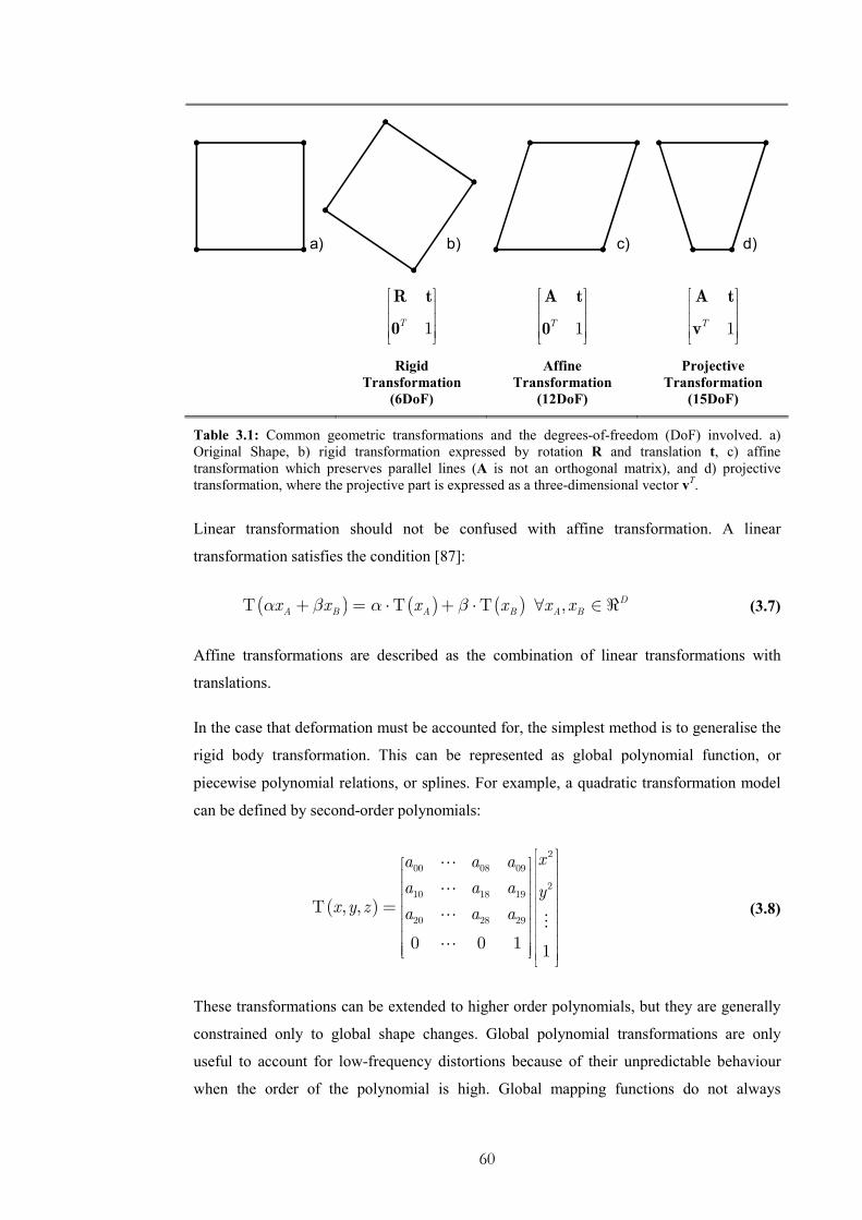
60
a) b) c) d)
1T
R t
0
1T
A t
0
1T
A t
v
Rigid
Transformation
(6DoF)
Affine
Transformation
(12DoF)
Projective
Transformation
(15DoF)
Table 3.1: Common geometric transformations and the degrees-of-freedom (DoF) involved. a)
Original Shape, b) rigid transformation expressed by rotation R and translation t, c) affine
transformation which preserves parallel lines (A is not an orthogonal matrix), and d) projective
transformation, where the projective part is expressed as a three-dimensional vector vT.
Linear transformation should not be confused with affine transformation. A linear
transformation satisfies the condition [87]:
( ) ( ) ( )A B A Bx x x xα β α βΤ + = ⋅Τ + ⋅Τ , D
A Bx x∀ ∈ ℜ (3.7)
Affine transformations are described as the combination of linear transformations with
translations.
In the case that deformation must be accounted for, the simplest method is to generalise the
rigid body transformation. This can be represented as global polynomial function, or
piecewise polynomial relations, or splines. For example, a quadratic transformation model
can be defined by second-order polynomials:
( )
2
00 08 09
210 18 19
20 28 29, ,
0 0 1 1
xa a a
a a a yx y z a a a
Τ =
(3.8)
These transformations can be extended to higher order polynomials, but they are generally
constrained only to global shape changes. Global polynomial transformations are only
useful to account for low-frequency distortions because of their unpredictable behaviour
when the order of the polynomial is high. Global mapping functions do not always
61
adequately capture anatomical deformation that is intrinsically local. Therefore, it is
difficult to use a parameterized transformation to describe local anatomical shape
variability.
3.4 Non-Rigid 2D/3D Registration
A non-rigid transformation can be described as a combination of a global and a local
component [89]:
( ) ( ) ( ), , , , , ,global localx y z x y z x y zΤ = Τ +Τ (3.9)
The global deformation component describes the overall deformation of the object. It is
usually either rigid or affine. The local transformation describes local deformation that
cannot be modelled as linear. The level of non-rigid deformation depends on the resolution
of the control points and is also directly related with the computational complexity. The
transformation model plays a major role in non-rigid image registration. Since the local
component encodes variability, it is inherently related to the notion of deformable models.
However, it should be noted that deformable models describe both shape and shape
variability, whereas a transformation is only a mapping mechanism from one image to the
other.
There are a number of transformation models that have been proposed in the literature for
non-rigid registration. Their formulation is also dependent on whether an intensity or
feature-based similarity measure is employed. Intensity based techniques iteratively
optimise the similarity between the corresponding voxels or pixels of the source and target
images. They transform the image at each iteration by using the current estimate of Τ to
evaluate the similarity measure, and the type of interpolation used can alter the solution
obtained.
In computer guided interventions, surface based registration is also common as surface
rendering requires less computational resources (CPU, RAM) than volume rendering. In
general, surfaces provide more redundancy than landmarks and this redundancy can be
useful for characterizing non-rigid motion. Furthermore, surface-based approaches are
more useful for aligning partially overlapped objects.
62
3.4.1 Transformation Models for Non-Rigid Registration
Non-rigid (also called non-linear) transformations are often used to describe
transformations with higher degrees-of-freedom than that of an affine transformation.
These transformations are meant to model local changes in the shape of an object. Thus far,
a number of models have been proposed which include those based on geometric
primitives, such as Thin-Plate Splines, B-splines, Multiquadric, Piecewise Linear and
Weighted Mean representations, and those based on physical models such as elastic, fluid,
finite element models and mechanical models.
Most non-rigid registration algorithms based on a non-physical transformation rely on the
use of a set of control points between the two image domains. These control points can
either correspond to particular features extracted in images or be regularly spaced within
the spatial domain. The transformation either interpolates or approximates the displacement
required to map each control point of the source image to the corresponding control point in
the target image. An interpolation condition arises when the number of control points is
equal to the number of unknown terms in the transformation function. Subsequently, the
system of equations that describes the transformation is fully determined. When the number
of control points is greater than the number of unknown parameters, only approximate
transformation coefficients can be derived. This implies that residual errors may exist
between the corresponding control points.
In physically-based transformations, model-based techniques are used to model the shape
and the dynamic behaviour of the surface. Such methods generally compute curve and
surface motion not by explicit matching, but by implicit consideration of image motion in
the form of virtual forces.
3.4.1.1 Spline Based Transformations
A spline-based transformation provides a smoothly varying displacement field, which, for
example, can be formulated as three thin-plate spline functions [87]:
( )1 2 3, ,T
t t tΤ = (3.10)
Thin-plate splines are defined as a combination of n radial basis functions ϑ .
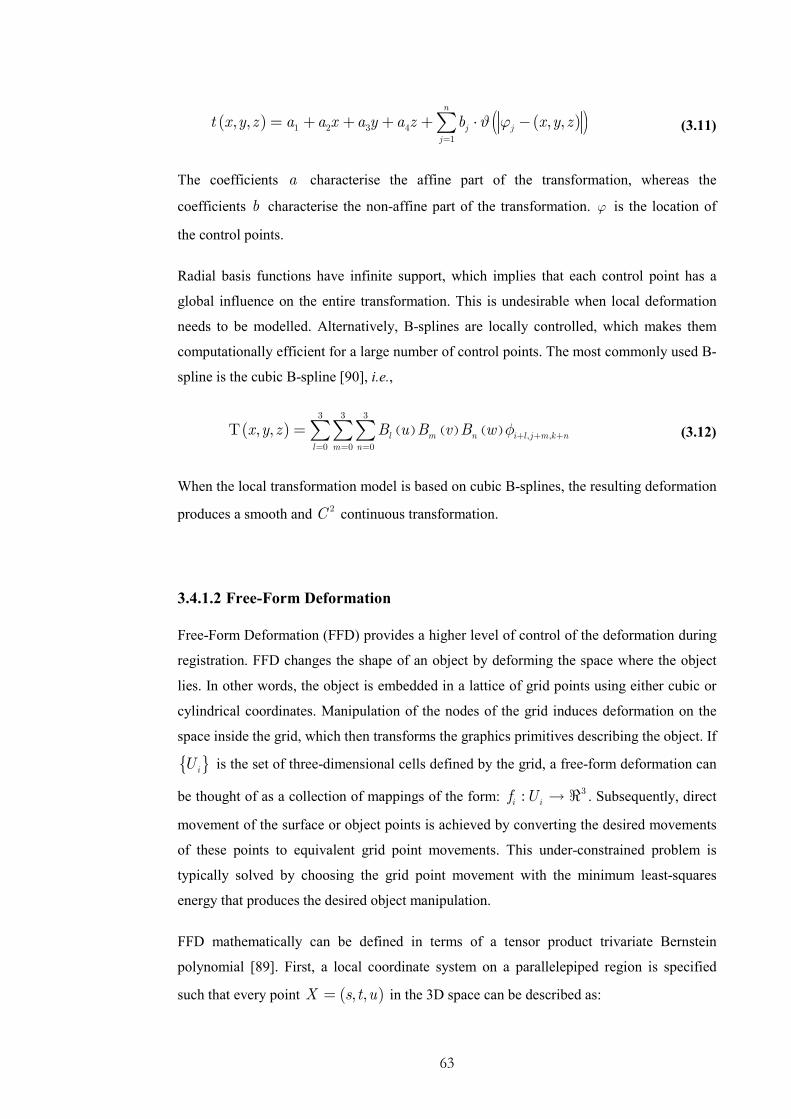
63
( ) ( )( )1 2 3 41
, , , ,n
j j
j
t x y z a a x a y a z b x y zϑ ϕ=
= + + + + ⋅ −∑ (3.11)
The coefficients a characterise the affine part of the transformation, whereas the
coefficients b characterise the non-affine part of the transformation. ϕ is the location of
the control points.
Radial basis functions have infinite support, which implies that each control point has a
global influence on the entire transformation. This is undesirable when local deformation
needs to be modelled. Alternatively, B-splines are locally controlled, which makes them
computationally efficient for a large number of control points. The most commonly used B-
spline is the cubic B-spline [90], i.e.,
( ) ( ) ( ) ( )3 3 3
, ,0 0 0
, , l m n i l j m k n
l m n
x y z B u B v B w φ + + += = =
Τ =∑∑∑ (3.12)
When the local transformation model is based on cubic B-splines, the resulting deformation
produces a smooth and 2C continuous transformation.
3.4.1.2 Free-Form Deformation
Free-Form Deformation (FFD) provides a higher level of control of the deformation during
registration. FFD changes the shape of an object by deforming the space where the object
lies. In other words, the object is embedded in a lattice of grid points using either cubic or
cylindrical coordinates. Manipulation of the nodes of the grid induces deformation on the
space inside the grid, which then transforms the graphics primitives describing the object. If
iU is the set of three-dimensional cells defined by the grid, a free-form deformation can
be thought of as a collection of mappings of the form: 3:i if U → ℜ . Subsequently, direct
movement of the surface or object points is achieved by converting the desired movements
of these points to equivalent grid point movements. This under-constrained problem is
typically solved by choosing the grid point movement with the minimum least-squares
energy that produces the desired object manipulation.
FFD mathematically can be defined in terms of a tensor product trivariate Bernstein
polynomial [89]. First, a local coordinate system on a parallelepiped region is specified
such that every point ( ), ,X s t u= in the 3D space can be described as:

64
0X X sS tT uU= + + + (3.13)
Every point inside the parallelepiped conforms to the following constraints: 0 1s< < ,
0 1t< < , 0 1u< < . Subsequently, the location of the control points is defined as:
, , 0i j k
i j kP X S T U
l m n= + + + (3.14)
where 1l + , 1m + and 1n + are the number of the grid planes in the S , T and
U directions, respectively. The deformation is specified by moving the control points away
from their original positions. The deformed position dX of an arbitrary point X is derived
by evaluating the vector valued trivariate Bernstein polynomial:
( ) ( ) ( ) , ,0 0 0
1 1 1l m n
l i m j n ki j k
d i j k
i j k
nmlX s s t t u u P
ji k− − −
= = =
= − − − ⋅ ∑ ∑ ∑ (3.15)
This deformation can also be formulated in terms of other polynomial bases, such as tensor
product B-splines.
FFD is a versatile tool for representing different geometric deformations. For example, a
parametric surface remains parametric after deformation. Furthermore, it is possible to
apply two or more FFDs in a piecewise manner so as to maintain the cross-boundary
derivative continuity. Another reason that FFD is so useful in solid modelling is that it
provides control over the volume change of the deformable object. In general, the volume
change is given by the Jacobian of the FFD. Therefore, by imposing a bound on the
Jacobian over the region of deformation also results in a bound of the volume change. Such
a bound is easily provided when the Jacobian is expressed as a trivariate Bernstein
polynomial. Subsequently, the two extremes of the coefficients provide upper and lower
bounds on the volume change. Thus far, FFD has been successfully used for 3D-3D image
registration for a number of applications [91]. Unlike radial basis functions, FFD requires a
regular mesh of control points with uniform spacing. Subsequently, its applications are
limited to volumetric images and solid object representations.

65
3.4.1.3 Physical Transformation Models
Physically-based techniques simulate natural motions and shape deformations based on
mathematical models that specify the physical behaviour of the object. Usually, they are
characterised by a high accuracy at the cost of a higher complexity. Elastic, viscous fluid
and biomechanical models belong to this category. The idea behind elastic transformations
is that the underlying deformation is a physical process that resembles the stretching of an
elastic material. This process is governed by both internal and external forces. The internal
force is caused by the deformation of elastic material and is opposite to the force that
deforms the elastic body from its equilibrium. The deformation of the object stops when all
the forces acting on the object form an equilibrium solution, which is described by the
Navier linear elastic Partial Differential Equation (PDE) [87]:
( ) ( ) ( )( ) ( )2 , , , , , , 0x y z x y z x y zµ λ µ∇ + + ∇ ∇ + =u u f (3.16)
where u describes the displacement field, f is the external force acting on the elastic
object, ∇ denotes the gradient operator, and 2∇ is the Laplacian operator. The parameters
µ and λ are Lame’s elasticity constants, which describe the behaviour of the elastic body.
The external force drives the registration process and it can be defined as the gradient of an
intensity-based similarity measure or the distance between curves, surfaces and anatomical
structures.
Fluid registration enables the modelling of highly localised deformations including corners.
Fluid registration, similarly to elastic registration, is described by the Navier-Stokes partial
differential equation:
( ) ( ) ( )( ) ( )2 , , , , , , 0x y z x y z x y zµ λ µ∇ + + ∇ ∇ + =v v f (3.17)
where v describes the velocity field. The relationship between the Eulerian velocity v and
the displacement field u is:
( )( )
( ) ( ), , ,
, , , , , ,x y z t
x,y,z,t x y z t x y z tt
∂= + ⋅∇
∂u
v v u (3.18)
One way to solve these partial differential equations is the Finite Element Methods (FEM).
These are numerical techniques that discretise the continuum into a number of elements in
order to approximate the continuous body equations over each element. FEM is
computationally intensive, and thus realistic deformation cannot be achieved in real-time.
Mass-spring-damper systems, Boundary Element Method and Finite Difference Method

66
(FDM) are also used to model physical deformable objects [92]. In Boundary Element
Method only the object boundary is considered. Although the resulting system is one
dimension less than FEM, it is still very dense and can not model internal behaviour of non-
homogeneous materials. In FDM, the differential operator is approximated by algebraic
difference operators. FDM is efficient and accurate when the geometry of the problem is
regular, but discretisation becomes extremely dense when it is used to approximate the
boundary of an irregular object.
Generally, FEM is superior when handling geometric approximations, because it uses the
exact differential operators that apply only in subspaces of the solution fields. Many
different approaches have been proposed in order to improve the time efficiency of FEM
[93]. The key to the efficient solution of this problem is the placement of nodal points and
elements that constitute the 3D mesh. For example, regions with large gradients need a
higher mesh density. In order to obtain an optimal mesh, every element should contain the
same predefined allowable error. Adaptation in FEM is essential to the performance of the
algorithm while maintaining local deformation details.
The main problem of physically-based transformations is that µ and λ are characteristic
parameters of the biomechanical tissue properties and they need to be measured prior to the
registration process. These parameters differ from subject to subject and they have a high
degree of intra-subject variability. These measurements also differ for in vitro and in vivo
specimens. Another problem associated with physically-based methods is the large number
of degrees-of-freedom involved, which makes the optimisation process difficult to
converge, thus leading to mis-registration errors.
3.4.2 Surface Representation and Deformable Models
Surface representation is an important element of non-rigid 2D/3D registration. In medical
image segmentation, a cloud of points is often derived for the anatomical structure and it is
common to use triangulation to form a 3D mesh. One way to construct a surface
deformable model is to use scattered data interpolation techniques. The problem of
scattered data interpolation uses a continuous function that interpolates values that are
known only at some scattered points. Approaches to the interpolation of scattered data can
be classified as global and local methods. In global methods, the interpolated values are
influenced by all of the data and usually they are limited to small datasets because of the
computational complexity involved. In local methods, the interpolated values are only

67
influenced by the values at neighbouring points, and thus these methods are suited for
modelling larger datasets. While interpolation techniques construct functions that pass
through the given data points, data fitting schemes construct functions that maintain the
overall trend of the input data and they do not necessarily pass through all the input points.
Scattered data interpolation functions can be formed based on splines and patches. They
include, for example, Bezier curves, double quadratic curves, B-splines, rational B-splines
and non-uniform rational B-splines (NURBS). These methods can represent both planar
and 3D curves and relate 2D patches for specifying surfaces. In these representations, the
curve or surface is represented by a set of control points. Therefore, the shape of the object
can be adjusted by moving the control points to new positions. This parameter-based object
representation is computationally efficient and can support interactive modifications.
However, precise alterations of the curves or surfaces can be laborious and a perceptually
simple modification may require the adjustment of many control points [94].
A NURBS surface is a bidirectional parametric representation of an object. Points on a
NURBS surface are defined by two variables, u and v, representing the longitude and
latitude, respectively. Points defined in Cartesian coordinates (x, y, z) can easily be
converted into surface coordinates (u and v) and vice versa. The extraction of a NURBS
surface can be based on patient image data and it permits the representation of a surface at
any resolution. Furthermore, NURBS can be altered easily via affine or other
transformations for dynamic modelling, as well as capturing anatomical variations among
patients. The main disadvantages of the NURBS are the inherent mathematic complexity
and the relatively large number of parameters that need to describe a 3D surface. The added
complexity, however, is beneficial for modelling biological shapes [95].
3.5 Similarity Measures for Image-Based Registration
A key issue of non-Rigid 2D/3D registration is how to define the distance measure between
the 3D data and the 2D projection. Similarity measures are based on either intensity values
or geometrical features. Both techniques involve optimising a similarity measure, which
evaluates how close the 3D model is to the corresponding 2D video frame. Intensity based
techniques can be based on cross-correlation or mutual information, whereas feature based
techniques rely on the extraction of features from the model and their alignment to the
correspondent images. Feature based techniques generally involve the following steps: (1)
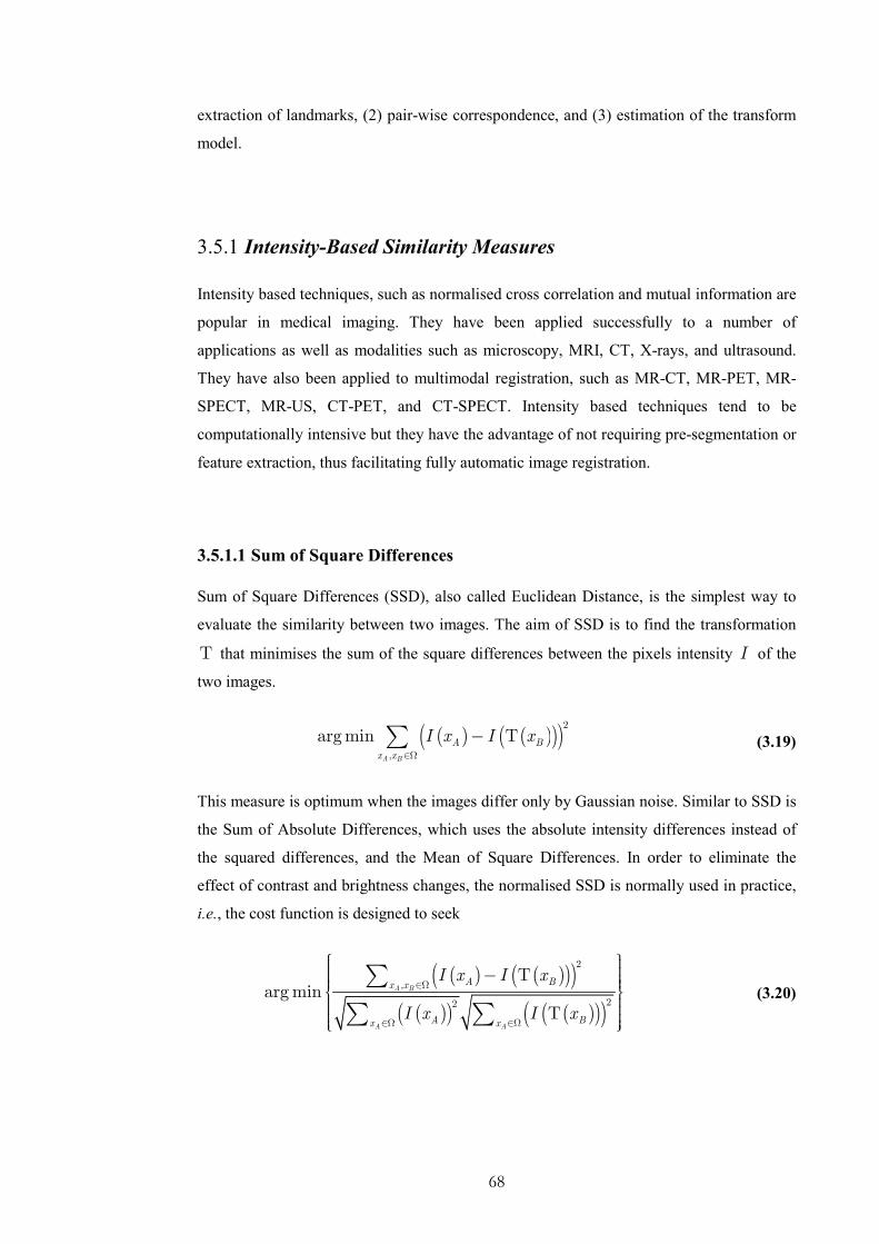
68
extraction of landmarks, (2) pair-wise correspondence, and (3) estimation of the transform
model.
3.5.1 Intensity-Based Similarity Measures
Intensity based techniques, such as normalised cross correlation and mutual information are
popular in medical imaging. They have been applied successfully to a number of
applications as well as modalities such as microscopy, MRI, CT, X-rays, and ultrasound.
They have also been applied to multimodal registration, such as MR-CT, MR-PET, MR-
SPECT, MR-US, CT-PET, and CT-SPECT. Intensity based techniques tend to be
computationally intensive but they have the advantage of not requiring pre-segmentation or
feature extraction, thus facilitating fully automatic image registration.
3.5.1.1 Sum of Square Differences
Sum of Square Differences (SSD), also called Euclidean Distance, is the simplest way to
evaluate the similarity between two images. The aim of SSD is to find the transformation
Τ that minimises the sum of the square differences between the pixels intensity I of the
two images.
( ) ( )( )( )2,
argminA B
A B
x x
I x I x∈Ω
− Τ∑ (3.19)
This measure is optimum when the images differ only by Gaussian noise. Similar to SSD is
the Sum of Absolute Differences, which uses the absolute intensity differences instead of
the squared differences, and the Mean of Square Differences. In order to eliminate the
effect of contrast and brightness changes, the normalised SSD is normally used in practice,
i.e., the cost function is designed to seek
( ) ( )( )( )( )( ) ( )( )( )
2
,
22argmin A B
A A
A Bx x
A Bx x
I x I x
I x I x
∈Ω
∈Ω ∈Ω
− Τ Τ
∑∑ ∑
(3.20)
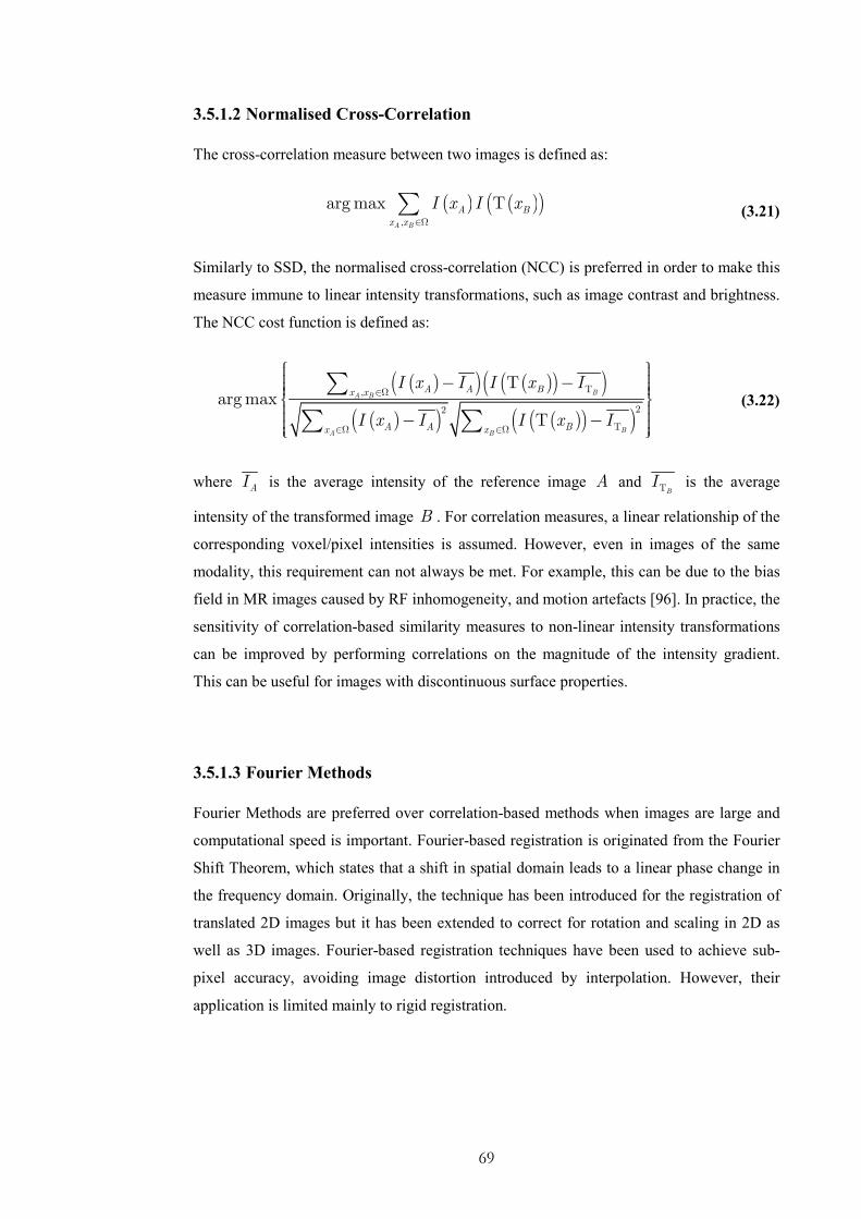
69
3.5.1.2 Normalised Cross-Correlation
The cross-correlation measure between two images is defined as:
( ) ( )( ),
argmaxA B
A B
x x
I x I x∈Ω
Τ∑ (3.21)
Similarly to SSD, the normalised cross-correlation (NCC) is preferred in order to make this
measure immune to linear intensity transformations, such as image contrast and brightness.
The NCC cost function is defined as:
( )( ) ( )( )( )( )( ) ( )( )( )
,
22argmax
BA B
BA B
A A Bx x
A A Bx x
I x I I x I
I x I I x I
Τ∈Ω
Τ∈Ω ∈Ω
− Τ − − Τ −
∑∑ ∑
(3.22)
where AI is the average intensity of the reference image A and B
IΤ is the average
intensity of the transformed image B . For correlation measures, a linear relationship of the
corresponding voxel/pixel intensities is assumed. However, even in images of the same
modality, this requirement can not always be met. For example, this can be due to the bias
field in MR images caused by RF inhomogeneity, and motion artefacts [96]. In practice, the
sensitivity of correlation-based similarity measures to non-linear intensity transformations
can be improved by performing correlations on the magnitude of the intensity gradient.
This can be useful for images with discontinuous surface properties.
3.5.1.3 Fourier Methods
Fourier Methods are preferred over correlation-based methods when images are large and
computational speed is important. Fourier-based registration is originated from the Fourier
Shift Theorem, which states that a shift in spatial domain leads to a linear phase change in
the frequency domain. Originally, the technique has been introduced for the registration of
translated 2D images but it has been extended to correct for rotation and scaling in 2D as
well as 3D images. Fourier-based registration techniques have been used to achieve sub-
pixel accuracy, avoiding image distortion introduced by interpolation. However, their
application is limited mainly to rigid registration.

70
3.5.1.4 Registration based on Geometrical Moment Invariants
Moment invariants were initially developed for positional invariant pattern recognition.
This is a convenient way of characterizing the geometric properties of objects in 2D or 3D
[97]. Other techniques, such as Gabor filters, wavelets and low frequency representations
can also be used to extract the geometric properties of the objects. For a 3D continuous
function ( )1 2 3, ,f x x x , the 3D regular moments of order ( )p q r+ + are defined by the
Riemann integrals:
( )( ) ( ) ( )22 2 2
1 2 3
, , 1 2 3 1 2 3 1 2 3, ,p q r
p q r
x x x R
M x x x f x x x dx dx dx
+ + <
= ∫∫∫ (3.23)
Although geometric moments operate directly on the image intensity values, they reduce
their content to a representative set of scalars and orientations [80]. Based on these
methods, the image centre of gravity and its principal orientation/principal axes are
computed from the first order moments. Subsequently, registration is performed by aligning
the centre of gravity and its principal orientations, also called invariant attribute vectors.
The notion of ‘invariant attribute vectors’ has been also used in [98] in the context of
surface registration. The goal is to distinguish different parts of a boundary according to the
shape properties. With this method, an attribute vector is attached to each vertex of the
model in order to reflect the geometric structure of the model from a local to a global level.
The attribute vector is an extension to curvature, which is invariant to rotation and
translation.
3.5.1.5 Mutual Information
Mutual Information (MI) is an entropy-based measure that was introduced in [99] to solve
the so called ‘sensor fusion’ problem. It uses a new information-theory approach for finding
the pose of an object based on a formulation of the joint entropy between the model and the
image. This is called Empirical Entropy Manipulation and Analysis. MI is an effective
method for image registration, particularly for multi-model applications. MI intuitively
encodes the statistical relationship of the voxel intensities, thus yielding more consistent
registration results.
Mathematically, MI of A and B is defined as the amount of information gained about A
when B is learned and vice versa. It is zero if and only if A and B are independent.

71
H(I1 ) H(I2) H(I1,I2)
MI(I1,I2)
Figure 3.2: The relationship between entropy and mutual information depicted as Venn diagrams.
The basic idea is that when images A and B are aligned, there will be a consistent
relationship between image A intensity and image B intensity. A transformation is
considered to be consistent if points that have similar intensities in image A are projected
to similar values in image B . A formal definition of consistency can be formulated based
on the principle of maximum likelihood. However, a similarity measure based on neighbour
likelihood alone suffers from certain drawbacks as it assumes that image A is a function
of image B , which may not be true in multi-modal images [100]. Furthermore, it may be
susceptible to outliers caused by occlusion and specularities.
Alternatively, Viola et al. [99] suggested using predictability and subsequently information
entropy based on the assumption that image A is predictable from image B but not
necessarily a function of the later. Information entropy, also called Shannon’s entropy or
marginal entropy describes how much uncertainty or randomness is encoded by a signal.
The more random a signal is, the higher the entropy. The entropy of a random variable x is
defined as:
( ) ( ) ( )lnh x p x p x dx≡ −∫ (3.24)
The joint entropy of two random variables x and y is defined as:
( ) ( ) ( ), , ln ,h x y p x y p x y dxdy≡ −∫ (3.25)
The concept behind image alignment using the joint entropy is that the predictability of one
image based on the other is maximised when the two images are aligned correctly and this
results in minimising the corresponding joint entropy. However, joint entropy is also
minimised when image intensities are constant, and thus the image by itself is easily
predictable. To overcome this problem, MI is expressed as the sum of the entropy of the
individual signals less their joint entropy:

72
( ) ( ) ( ) ( ), ,M x y h x h y h x y= + − (3.26)
The relation between entropy and mutual information can also be depicted using Venn
diagrams as shown in Figure 3.2, where MI is zero when two images are uncorrelated and
reaches maximum when they are registered to each other. The fact that MI is not minimised
by image constancy can be better shown by considering a transformation Τ that seeks to
align transform image B to A . The MI of the intensity values of the source image ( )AI x
and the transformed image ( )( )BI xΤ that takes the form:
( ) ( )( )( ) ( )( ) ( )( )( ) ( ) ( )( )( ), ,A B A B A BM I x I x h I x h I x h I x I xΤ = + Τ − Τ (3.27)
Registration algorithms based on MI of the images A and B seek to find a transformation
′Τ that maximises their mutual information over the domain of possible
transformationsΤ .
( ) ( )( )( ),arg max A BM I x I xΤ
′Τ = Τ (3.28)
In Equation (3.27), the first term of the MI equation expresses the entropy of the source
image A and it does not depend on the transformation Τ , hence it is constant for a given
set of images. The second term is maximised when the transformation Τ projects B into
the complex parts of image A and it is minimised when the transformation leads to
constant intensity. The last term of (3.27) encourages a transformation that maximises
predictability. Therefore, both the second and third terms strives to minimise entropy, while
avoiding a transformation that leads to constant image intensities.
Studhome et al [101] pointed out that MI is sensitive to the changes of image overlap. This
implies that a change in the proportion of the image overlap can result in changes of MI
that do not reflect the quality of alignment between the two images. For this reason, they
formulated the Normalised Mutual Information, which provides a measure that is
independent to the field of view.
( ) ( )( )( )( )( ) ( )( )( )( ) ( )( )( )
,,
A B
A B
A B
h I x h I xMN I x I x
h I x I x
+ ΤΤ =
Τ (3.29)
MI has been evaluated from a number of different groups [86, 96, 102]. Although it is
widely accepted as one of the most reliable similarity measures in multi-modal image

73
registration, it also has certain drawbacks. Problems usually arise due to poor image
resolution and small overlapping areas between the two images. MI can fail if the 2D
histogram is relatively sparsely populated, which is the case when image resolution is low.
This problem is also apparent in 2D/3D registration, since the number of pixels reduces
considerably when compared to 3D/3D registration [86]. Problems also arise when the
function contains many local minima [103]. Furthermore, MI decouples intensity values
and location information. As a result, the dependency of the intensity values on
neighbouring voxels/pixels is ignored [102]. In practice, incorporation of spatial
information can improve the robustness of the registration process. However, as MI only
relies on an analysis of the global intensity information, it is not well suited to tasks where
the statistical aspects of the intensity values vary within the image, which may be the case
for endoscopic images because of shadows and intensity gradients due to directional
illumination [104].
3.5.1.6 Beyond Mutual Information
Recently, several approaches have been introduced to complement or replace MI. For
example, in the work by Likar et al. [105] noted that searching for the global registration
transformation with a MI-based similarity measure is not practical for highly non-rigid
deformations. Typically, this approach leads to a complex similarity function that may have
many local maxima. They proposed to subdivide the image into blocks that can be
registered locally by a rigid or affine transformation. The registered images at a higher level
are then partitioned into progressively smaller sub-images. Once all the sub-images are
registered, a globally consistent registration is achieved by using the centres of the
registered sub-images as point pairs and an elastic thin-plate-spline interpolation. However,
the reduction of the number of samples due to the partition of the images into smaller sub-
images can reduce the statistical power of the joint intensity histogram. In order to improve
the probability estimation, random re-sampling is introduced, which prevents the alignment
of a too large number of grid points to minimise the interpolation artefacts.
Dinggang et al [98] also noted that minimising an intensity-based similarity measure does
not necessarily imply good registration of the underlying anatomy. In order to address this
problem, they proposed a new image registration approach based on a Hierarchical
Attribute Matching Mechanism (HAMMER). Their work has two main features. Firstly,
they use attribute vectors calculated from the tissue maps across different scales for each
voxel of the image. Secondly, in order to avoid being trapped by local minima, HAMMER

74
uses a successive approximation of the energy function optimized by lower dimensional
smooth functions. By hierarchically selecting the features that have distinct attribute
vectors, the ambiguity in establishing correspondence is significantly reduced.
In HAMMER, the transformation between two images is defined as a mapping of one
coordinate system to the other (rigid-body transformation) followed by a shape
transformation. Let ( )AI x be the intensity of voxel x in a template brain image, and
( )BI y be the intensity of voxel y in another brain image. Here, x and y are the 3D
coordinates of the voxels volumes AV and BV , respectively. The displacement field ( )u x
defines the mapping from the coordinate system of image A to image B , while
transformation ( ) ( )h x x u x= + defines the mapping that transforms image A into the
shape of image B . The inverse transformation is defined as ( )1h x−.
The hierarchical attribute matching mechanism for non-rigid registration uses a sequence of
lower dimensional energy functions to approximate the following multivariate energy
function:
( )
( ) ( ) ( )( )( )( )( )
( )
( )
( )( ) ( )( ) ( )( )( )
( )
( )
( )
( )
1
2
1 ,
1 ,
A
B
A
A B
z n xA
x V
z n x
A B
z n x
B
y V
z n x
x V
z m z h z
xz
z m h z z
yz
u x
ε α α
ωε
ε α α
ωε
β
∈
∈∈
−
∈
∈∈
∈
− Ε =
−+
+ ∇
∑∑ ∑
∑∑ ∑
∑
(3.30)
In the first term, the similarity of the attribute vectors for each template voxel x in its
spherical neighbourhood ( )n x is calculated. It is worth noting that the similarity is
estimated over a neighbourhood area, rather than on individual voxels. In (3.30), ( )A zα
and ( )B zα are the attribute vectors of the voxel z in image A and B , respectively.
Function ( )., .m measures the similarity of two attribute vectors within the range of 0 to 1.
In (3.30), the denominator ( )
( )z n x
zε∈∑ is used as a normalization factor. The parameter
( )A xω is the relative weight for each voxel x in image A . The voxels with the distinct
attribute vectors are assigned with larger weights, because they can be identified more
reliably than others. In a hierarchical registration scheme, these voxels drive the
deformation of the image A by initially focusing on the first term of the energy function.

75
The second energy term is similar to the first, but it is defined in the domain of image B
and it is used to constrain the inverse transformation ( )1h− ⋅ , from image B to A .
Compared to other techniques, the robustness of HAMMER is achieved through a
combination of the first two terms of the energy function, i.e., the first term is focused on
deforming image A to B , whereas the second is focused on deforming image B back to
A . The third term is a smoothness constraint on the displacement fields, where 2∇
denotes the Laplacian operator and the parameter β controls the smoothness of the
deformation field.
One important factor of HAMMER is the way that the attribute vector is defined. If it
contains rich enough information then it is possible to distinguish between different parts of
the anatomy, even when this cannot be inferred from the intensity values alone. Typically,
the attribute vector is defined for each voxel x in a volumetric image and it reflects the
anatomical structure at different scales. Therefore, an attribute vector ( )xα consists of
three vectors:
( ) ( ) ( ) ( )1 2 3x x x xα α α α = (3.31)
( )1 xα represents the edge type of the voxel x in the image and it is designed based on the
classification of tissue between the voxel x and its neighbouring voxel z . In this way,
prior knowledge about the image features and the type of the deformation is also
incorporated into the registration scheme. In (3.31), ( )2 xα represents the intensity of voxel
x with a range of grey levels. Finally, vector ( )3 xα represents the Geometrical Moment
Invariants (GMIs) of each tissue at different scales.
An intuitive way of using an intensity based approach to deal with 2D/3D registration has
been suggested in [106] for the alignment of 2D optical images with 3D surface data of the
human faces. In this work, registration is performed by optimizing a similarity measure
based on photo-consistency with respect to the transformation parameters. The concept of
photo-consistency can be summarised as follows. When the scene radiance is assumed to
follow a locally computable lighting model, which means that shadows, antireflections and
transparencies are not allowed, the observed intensity depends on the cosine of the angle
between the surface normal and the vector to the light source. Note that it does not depend
on the angle between the surface normal and the direction to each optical camera.
Therefore, a surface point projected into different image planes should yield identical
image intensities in all views. Given N images of the 3D model, a similarity measure is

76
defined in order to decide whether a point in one view corresponds to a point in the other.
The arithmetic mean of the pixel values associated with a given point is calculated over all
optical images. Subsequently, the mean squared image intensity differences are calculated
and a similarity measure based on a threshold value is introduced.
3.5.2 Feature-Based Techniques
Although the accuracy of intensity-based registration is usually better than feature-based
registration, in some cases intensity-based techniques can fail due to anatomical or scene
structure changes. Another important advantage of feature-based techniques is that they
converge faster because they use a reduced representation of the image. For this reason,
they are preferred when real-time response is necessary. These techniques have been
successfully applied to AR and surgical applications involving implanted fiducial markers.
3.5.2.1 Feature Detection
Feature detection depends on the nature of the application and plays an important role in
the accuracy of the registration. In general, features should be distinctive and efficiently
detectable in both images. They should also be fixed during the whole experiment and
sufficiently populated in the image plane. Possible features include landmarks and their
surrounding regions, curves, segmented sets, or points. In 2D/3D registration, the notion of
edges, regions or points needs to be generalised to 3D surfaces, such that a meaningful
match between 2D edges and 3D ridges is possible. To this end, a number of definitions
have been utilised to accomplish this, which also reveals that a mapping between the 2D
and 3D feature space is not trivial.
In these approaches, regional features are mainly selected by segmentation and they should
ideally be invariant to scale, rotation, and illumination changes. Curve and line selection is
also popular. Standard edge detection methods, such as Canny detector, are often employed
in 2D/2D registration [78]. However, they are usually not appropriate for 2D/3D
registration as salient curves on the 3D model surface may not have an accurate match in
the 2D image data. In the work by Pennec et al. [107], features of the 3D volume data are
identified through differential geometry where ridges are extracted from the medial axis
transform. It is worth noting that this definition does not represent salient curves on a
surface.

77
Crest and extremal lines describe the loci of the surface where one of the principal
curvatures reaches a local minimum/maximum along the principal curvature. Directional
curvatures at a surface point P are defined by the intersection of the plane ( )1, ,P t n with
the surface at point P , where n is the normal to the surface point P and 1t presents the
principal direction, which is the extremum of the surface curvature at point P .
Subsequently, a crest line can be extracted as the intersection of two implicit surfaces
[107]:
f I= and 1 0e = (3.32)
where f represents the intensity value of the image and I is an iso-intensity value. In
(3.32), 1 1 1e k t= ∇ ⋅ and it is called the extremality function.
Extremal points are close to the notion of corner points. They can also be identified along
the same line as extremal lines. Extremal points are defined as the intersection of three
implicit surfaces [107]:
f I= and 1 0e = and 2 0e = (3.33)
Similarly to 1e , 2e is defined as 2 2 2e k t= ∇ ⋅ where 2k is the associated principal
curvature. In 2D images, the point features are typically extracted as the intersection of
salient lines. In general, feature based methods are sensitive to feature extraction and
selection. Although various techniques have been developed for automatic feature
selection, a certain amount of user interaction is often required.
3.5.2.2 Feature Correspondence and Pose Determination
In feature-based registration, both correspondence between extracted features and pose
should be determined. Usually they are tackled simultaneously in an iterative manner.
Features are treated as points either by extracting the geometric centroids or by assuming
that curves and lines are comprised of a set of points. The problem of establishing
correspondence between two sets of points is not trivial especially when noise and localised
deformation are present. In general, the set of points may be unequal in size and can differ
due to non-rigid transformations. Point correspondence usually is formulated as a discrete
linear assignment problem and the pose estimation is considered as a continuous least-
squares problem. The combination of the two makes the non-rigid point registration
78
problem difficult. Thus far, a number of approaches have been developed to tackle these
issues. The Iterative Closest Point (ICP) algorithm is one of the popular techniques to
register 3D point clouds, curves and surfaces.
ICP is an iterative approach that identifies the optimal transformation between 3D shapes
[besl92]. During each iteration, the algorithm establishes point correspondence by
identifying for each point on the reference surface the closest point in the target surface.
Typically, ICP uses a mean square distance metric over all six degrees-of-freedom and the
algorithm can converge monotonically to the nearest local minimum. However, it requires
an initial pose that is close to the solution in order for the algorithm to converge. In the case
of large non-rigid deformation, the ICP algorithm does not always converge to the global
minimum. This is due to the fact that ICP uses a crude way to assign correspondence,
which can generate local minima and cannot guarantee one-to-one correspondence.
Subsequently, its performance can deteriorate with the presence of outliers.
As an alternative, Chui et al. suggested the use of an energy function to solve both the
correspondence and the transformation problem for non-rigid registration [108]. They
point out that solving for binary, one-to-one correspondences and outliers at each step is not
meaningful when the transformation is far away from the optimal solution. To cater for the
uncertainty of whether a point matches with another, one allows fuzzy, partial matches
between the two sets of points. This is the basic idea of softassign, which has also been
used in [109]. In other words, the discrete problem is now turned into a continuous one in
order to avoid getting trapped in a local minimum. Softassign has emerged from neural
networks and it is concerned with how to assign fuzzy values in a set of variables in order
to form a doubly stochastic matrix. Doubly stochastic matrix is a square matrix with all
positive entries with rows and columns summed to one. It has been proved that a doubly
stochastic matrix is obtained from any square matrix with all positive entries by the
iterative process of alternating row and column normalisations. This is known as the
assignment problem, which is a classical problem in combinatorial optimisation. However,
non-rigid point-matching problem is much harder than the linear assignment problem,
which can be solved in polynomial time.
Another useful optimisation technique, called deterministic annealing, can also be used to
directly control the fuzziness by adding an entropy term to the energy function, called
temperature [108]. Higher temperature values correspond to a higher degree of fuzziness in
correspondence. The minima obtained at each temperature are used as initial conditions for
the next stage as the temperature is lowered. The resulted energy function expresses both
the correspondence and the pose problems at once and it is formulated as:
79
( ) 2
1 1
,
1 1 1 1
arg min
log
N K
ba b a
a b
N K N KM f
ba ba ba
a b a b
m v f u Lf
m m m
λ
ζ
= =
= = = =
− + + +Τ −
∑∑
∑∑ ∑∑ (3.34)
In the above energy function, two point sets U and V are defined in , 2, 3n nℜ = , so they
consist of points , 1,2,...,aU u a N≡ = and , 1,2,...,bV v b K≡ = . The non-rigid
transformation is represented by function f , where 2
Lf is a smoothness term that
imposes constrains on the mapping function. In (3.34), [ ]0,1bam ∈ and it is the fuzzy
correspondence matrix which satisfies:
1
1
1N
ba
a
m+
=
=∑ for 1,...,b K∈ and 1
1
1K
ba
b
m+
=
=∑ for 1,...,a N∈ (3.35)
whereΤ is the temperature and it is followed by the entropy term. In (3.34), the last term is
the robustness control term that prevents the rejection of too many points as outliers.
Although this formulation is limited to the alignment of 2D or 3D point sets, it can also be
extended to registering data from different dimensions and modalities.
When it comes to 2D/3D registration, the perspective projection should also be taken into
account. Existing approaches have addressed the problem of registering a 3D model and its
perspective projection using a combination of the softassign technique for the problem of
correspondence [110, 111]. It incorporates an iterative technique called Pose from
Orthography and Scaling with Iterations (POSIT) for pose estimation. The basic principle
of POSIT is based on the fact that the pose problem for perspective projection can be
solved by iteratively refining the pose computed for scaled orthographic projection.
According to the idea of ‘softassign’, the correspondence between image features and
model features in the global objective function is expressed as a correspondence matrix in
which each term is a weight for the match between an image point and a model point. This
weight is a function of the distance between the scaled orthographic projection of the model
point and the scaled orthographic projection after that model point is displaced onto the line
of sight of the image point (for a camera pose that is refined during the iteration process).
For the pose problem, scaled orthographic projection is used as an approximation of
perspective projection, because it allows one to solve the pose problem with linear algebra
and with fewer unknowns than with projective geometry.

80
3.6 Optimisation Techniques
Most of the image registration approaches involve an optimization step. Optimisation
techniques are iterative processes for identifying the optimal transformation that maximizes
the similarity between the two images/data sets. This is not an easy task especially when the
transformation has large degrees-of-freedom and the similarity measure exhibits many local
minima. Subsequently, the selection of an appropriate search space is crucial. In practice,
the search space is affected by the similarity measure, the type of the transformation, and
the image data involved.
Based on the similarity measure and the nature of transformation, a cost function can be
constructed. Subsequently, global or local optimization techniques are used to minimize the
cost function. Global optimization techniques are used to find the best set of parameters to
optimize an objective function. One such method is the simulated annealing algorithm,
which is a generalization of a Monte Carlo method applied to combinatorial optimization
problems. Local optimization methods, on the other hand, usually converge faster but they
cannot guarantee a global optimum solution. These methods include Powell’s method,
Simplex, and Gradient Descent Algorithms. In these approaches, only information about
the neighbourhood of the current approximation is used and subsequently, the algorithm is
expected to converge to a local minimum/maximum close to the initial position.
3.7 Evaluation of 2D/3D Registration Algorithms
In image guided surgery, registration errors can have major consequences in patient
safety. The quantification of the registration quality is also an important issue. For
example, registration errors can have a strong influence on the quantification of the
lesion progression and mis-alignment of important anatomical structures. Accurate
evaluation of the performance of 2D/3D registration algorithms is of crucial importance in
surgical guidance. Currently, there is a lack of a consistent, common scheme that would
permit an objective, direct, and data-invariant comparison between different registration
methods. Thus far, most techniques have been developed under the strict constraints of a
particular application framework with lack of general applicability. Kraats et al [112]
investigated this issue and introduced a standard validation method based on the 3D
Rotational X-ray imaging system. However, this system is designed to address only the

81
problem of registering 3D CT with X-ray images. Otherwise, the ground truth data cannot
be evaluated with this method and the target-registration error cannot be estimated.
The most fruitful part of this work is the criteria of validation, which can be applied to other
registration problems. These are the ground truth data and the determination of accuracy.
Although the availability of common datasets is necessary in order to establish a
standardized evaluation framework, ground truth data are not always available. Usually, the
ground truth data can be created under a controlled environment with additional tracking
devices. The determination of accuracy involves the estimation of validation statistics under
a range of different starting positions and experimental conditions.
In the case of bronchoscopy registration, 2D/3D algorithms have been investigated by a
number of research groups [74, 75, 77, 113, 114]. However, a common framework for
validating these algorithms has yet to be created. For example, Mori et al. [75] used visual
inspection to decide whether a frame was successfully registered. In this way, there is no
quantitative measurement of the error involved and an indication of the sensitivity of the
algorithm to different registration parameters. In the work presented by Helferty et al., a
rubber mould from a human airway tree was used to assess a biopsy procedure and average
positional error between a target metal bead and the needle. However, there is no
systematic assessment of the angular accuracy of the technique. The exploration of the
influence of different initialisations on the convergence of the algorithm is presented in
[77], although the notion of the ‘ideal registered position’ and ‘registration error’ has not
been fully clarified.
3.8 Discussion and Conclusions
Image-based registration is a valuable tool for monitoring the progression of diseases,
surgical planning, and intra-operative guidance. In general, image registration consists of
four major components. These include the target and source datasets, the transformation
model, a similarity measure, and an optimisation technique. The choice of the
transformation model and the similarity measure plays a key role in the success of
registration techniques and this will be the focus of the work presented in this thesis.
For free-form deformation, transformation can be described by a local and global
component. The local component encodes the variability of the model and a number of
82
geometrical- and physical-based models have been proposed. Geometrical-based models
offer a large number of unrestricted control points but it may be difficult to adjust in
practice. Physical-based models provide an effective way of modelling the physical
behaviour of complex structures. However, their application requires accurate measurement
of the tissue properties, which in practice can be difficult.
For image registration, similarity measures can be classified as intensity-based and feature-
based approaches. Intensity-based techniques compare image intensities without structural
analysis, whereas feature-based techniques are dependent on the extraction and matching of
features of the reference and target images. Intensity based techniques have a number of
limitations. For example, cross-correlation based methods are sensitive to intensity changes
introduced by varying illumination and changing modality. When applied to endoscopic
image registration, careful adjustment of illumination condition is important to the accuracy
of the registration result. Mutual information is based on the statistical dependency between
datasets and thus is more suitable for registering multi-modal images. However, it can fail
when the histogram is sparsely populated, which is typical for 2D/3D registration. A major
disadvantage of intensity-based techniques is that image similarity does not necessarily
imply correct registration. In practice, feature based approaches can augment the
registration performance but the robust extraction of salient features used for registration
can be a difficult task.
Despite extensive research in registration, non-rigid 2D/3D registration remains a
challenging issue. This is partly due to the ill-posed nature of the problem as well as the
difficulty in handling both global and local deformation. For this reason, most existing
techniques reduce the problem to a 2D/2D registration scheme by using the 2D projections
of the 3D data. However, this procedure introduces further ambiguity when deformation is
present. In the next chapter, we will demonstrate that for bronchoscopy navigation, it is
possible to exploit the unique camera-lighting configuration of the system to provide a
robust surface geometry based 2D/3D registration algorithm. We will demonstrate why the
proposed method is superior to existing techniques and how it handles significant lighting
condition changes during bronchoscope examination.

83
Chapter 4
2D/3D Registration based on pq-based
Representation
egistration of 2D bronchoscope video to 3D tomographic data is a popular research
topic in medical imaging due to improved imaging hardware in recent years. For
example, the work by Helferty et al. [113] analysed preoperative CT data of the airways to
compute a segmentation of the tracheo-bronchial tree and the centrelines through the major
airways. In this way they used the centrelines as a path to guide the registration process. In
this method, the similarity measure is based on Normalised Mutual Information, which is
calculated from weighted entropy terms, estimated from the normalised image histograms
of the video and CT reconstructed images. Their hypothesis is that the darker pixel values
have less noise and are more likely to form a match in the two images. In other words, dark
areas give more useful information, as they correspond to distal lumen and airway
bifurcations.
In the work by Bricault et al. [77], a multilevel strategy was adopted by considering the fact
that the bronchial lumen presents no specific texture and gray values vary with the camera
position and lighting conditions. In order to enhance the robustness of the algorithm, a
model-based shape-from-shading algorithm is used to reconstruct the surface of the lumen
and the subsequent 2D/3D registration is transformed into a 3D/3D registration problem.
Recently, Mori et al [74] presented a registration method that does not depend on the
airway structure. The objective of the work was to develop a general framework for
tracking the viewpoint and view direction of the fiberscope in relation to the 3D model. The
method searches for the best viewpoint and view direction by calculating a matching ratio
R
84
between a reconstructed virtual bronchoscopic image and a real one. Camera motion is also
estimated by extracting optical flows. Optical flows of a video sequences are the velocity
fields that indicate the motion of objects from one frame to the other. For this method, since
a cross-correlation based similarity measure was used, the lighting properties of the 3D
model played an important role in the registration process. If the lighting is not carefully
adjusted to match to that of the bronchoscope video, cross-correlation based similarity
measures can fail. In real endoscopy, the illumination power decreases with the square of
the distance from the light source. To simulate this effect, the parameters are adjusted
manually such that similar visual appearance can be achieved. Throughout the registration
process, the specular and reflection properties of the tissue are ignored.
Since image registration often depends on the inherent characteristics of the image data, it
is necessary to exploit the unique constraints of the image formation process to facilitate
faster and more accurate convergence of the registration algorithm. These special
conditions, although may not be generally true, can reduce the ambiguity of the otherwise
ill-posed problem. In this chapter, a hybrid approach is proposed. It is based on the
extraction of surface normals from the bronchoscope video images by using the camera-
lighting constraint of the bronchoscope. The components of these normals can be
represented in the ( ),p q gradient space that expresses the slopes of the surface in the x and
y directions as shown in Figure 4.1. This permits the development of a linear shape-from-
shading technique to derive the 3D geometry of the 2D bronchoscope data such that
registration can be performed based on the alignment of the surface normals. In this way,
there is no need to adjust the lighting of the 3D model, and hence significantly increases the
robustness of the registration algorithm.
The basic process of the proposed technique involves the following steps. Firstly, the
surface normal for each pixel of the 2D video bronchoscope image is extracted by using a
linear local shape-from-shading algorithm based on the camera/lighting constraint of the
bronchoscope. The corresponding pq vectors of the 3D tomographic data are calculated
from direct z-buffer differentiation. Subsequently, a similarity measure based on angular
deviations of the pq vectors derived from 2D and 3D data sets is used to find the optimal
pose of the camera in relation to the 3D model, thus establishing the correspondence
between the 2D video and the 3D tomographic data.
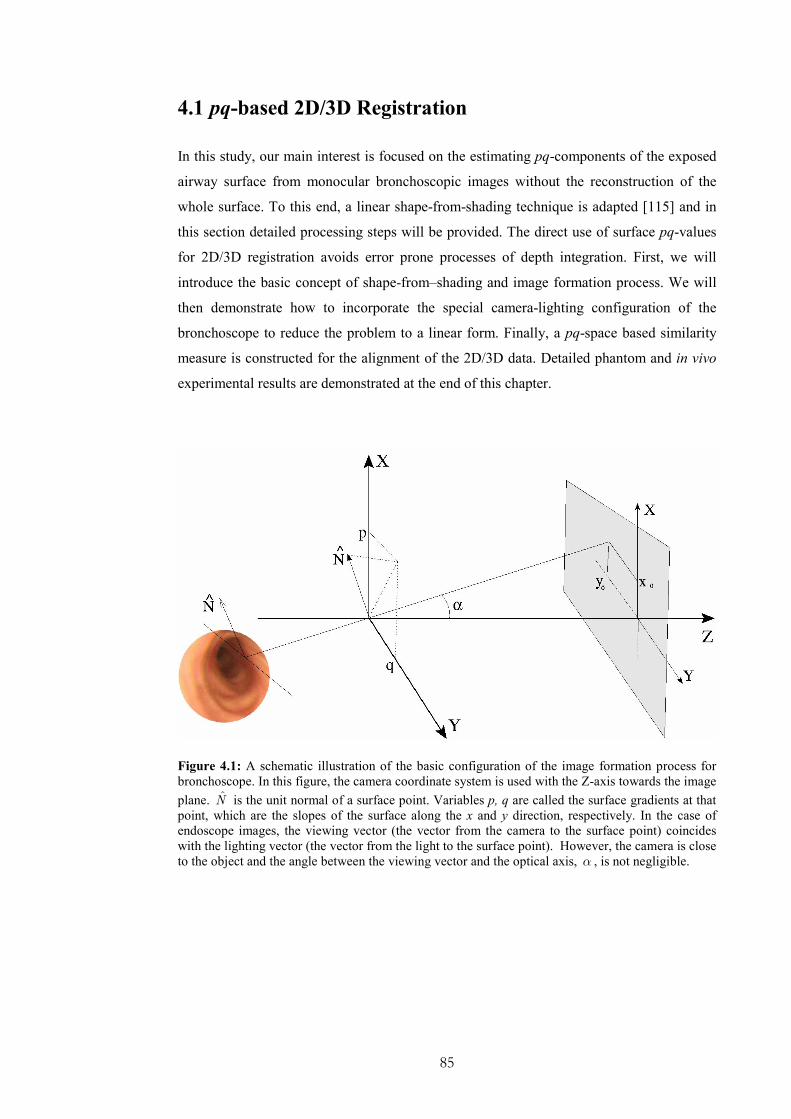
85
4.1 pq-based 2D/3D Registration
In this study, our main interest is focused on the estimating pq-components of the exposed
airway surface from monocular bronchoscopic images without the reconstruction of the
whole surface. To this end, a linear shape-from-shading technique is adapted [115] and in
this section detailed processing steps will be provided. The direct use of surface pq-values
for 2D/3D registration avoids error prone processes of depth integration. First, we will
introduce the basic concept of shape-from–shading and image formation process. We will
then demonstrate how to incorporate the special camera-lighting configuration of the
bronchoscope to reduce the problem to a linear form. Finally, a pq-space based similarity
measure is constructed for the alignment of the 2D/3D data. Detailed phantom and in vivo
experimental results are demonstrated at the end of this chapter.
Figure 4.1: A schematic illustration of the basic configuration of the image formation process for
bronchoscope. In this figure, the camera coordinate system is used with the Z-axis towards the image
plane. N is the unit normal of a surface point. Variables p, q are called the surface gradients at that
point, which are the slopes of the surface along the x and y direction, respectively. In the case of
endoscope images, the viewing vector (the vector from the camera to the surface point) coincides
with the lighting vector (the vector from the light to the surface point). However, the camera is close
to the object and the angle between the viewing vector and the optical axis, α , is not negligible.

86
4.2 Shape-from-shading
Shape-from-shading is a classic problem in computer vision that has been well investigated
since the pioneering work of Horn [116]. It addresses the problem of extracting both
surface and relative depth information from a single image. Before we move on to the
special case of extracting surface information from bronchoscopic images, we need to
define a few basic concepts of how image intensity is related to scene geometry. To extract
the 3D structure from a monocular image, it is also important to study how the brightness
pattern of an image depends on the shape of the object being imaged. Most of the notations
used in this chapter follow the convention adopted by Horn on his original work on Shape-
from-shading and photometric stereo [116-118].
4.2.1 Human Vision and Depth Perception
How the human visual cortex infers depth information from 2D images is an issue that has
intrigued scientists and philosophers for centuries. There are many cues that help the vision
system to recover the third dimension. Well known cues for depth recovery include motion
parallax and binocular disparity. Motion parallax is the apparent shift of an object against
the background. Binocular disparity, on the other hand, is the difference between the
relative positions of corresponding features resulting from the spatial separation of the two
eyes.
When an image is projected onto the screen, the apparent depth information is lost.
However, humans can still infer shape from monocular images with a remarkable degree of
details [119]. It is believed that the extraction of shape-from-shading is a visual process,
developed prior to higher-level cognitive tasks, such as perceptual grouping and motion
perception [120]. The leading cue in a monocular image is the variations in brightness, also
called shading. Shading should not be confused with shadowing, which is the locus of
points where the rays graze the surface (self-shadow), or a region of darkness where light is
blocked (cast-shadow). Shading arises partly from the fact that the fraction of the light
source that appears at a particular point on the surface depends on surface orientation.
Subsequently, shading provides cues all over the surface and not just along special
contours. However, shading is related to shadowing in the sense that shadowing of parts of
the microstructure of the surface may contribute to the shading effects apparent on the
macro scale.
87
The recovery of shape-from-shading is by no means trivial, since the problem is ill-posed.
Simply speaking, the orientation of an object located at a given distance from the camera
depends on two parameters while there is only one measurement of brightness for each
pixel. Therefore, to solve the shape-from-shading problem mathematically, additional
constraints must be adopted. One common way of providing these constraints is to assume
a smooth and continuous surface, implying that the surface orientations of the neighbouring
surface patches are not independent. It has been shown that for the human vision system,
object boundaries and prior knowledge plays an important role in resolving depth
ambiguities. We often simplify the task of interpreting shading by assuming a single light
source emitting light from above in relation to the retinal coordinates [119]. Furthermore, in
our visual environment, we mainly deal with opaque objects, where the light rays do not
penetrate through the material. Subsequently, we only need to focus on the surface of the
object. It is with these simplifications, that the 3D shape of an object can be recovered
given only one monocular image. To understand how to use the shape information encoded
in the intensity values of an image, it is important to study the relationship between the
light falling onto a surface and that radiated from the same point according to the
reflectance properties and orientation of the surface. It is also important to study image
formation process itself.
4.2.2 Understanding Image Intensities
The image of a 3D object depends on its shape, its reflectance properties, and the location
of the light sources. It is also a function of the position of the object relative to the camera
and the object’s orientation in space. Radiometry is the field that studies the measurement
of electromagnetic radiation, including visible light. It is central to the determination of
how the brightness at a particular point of the image is formulated. In this field, the amount
of light falling onto a surface is called the irradiance and the amount of light radiated from
a surface is called the radiance. Light transports energy through space and subsequently
brightness is determined by the amount of energy the imaging system receives per unit
area. The fact that a surface can anisotropically radiate into a whole hemisphere of possible
directions is what complicates the notion of radiance, and subsequently the process of
image formation. This is modelled with the Bidirectional Reflectance Distribution Function
(BRDF), which is a measure of how much of the incident light is reflected in a particular
direction. More accurately BRDF is the ratio of radiance to irradiance. Analytical

88
estimation of the reflectance function is difficult to construct, and hence it is usually
determined empirically.
Assuming a single point light source and a unique value of BRDF, which can be assumed
for most surfaces, the geometry of reflection is governed by three angles.
• The incident angle, which is the angle between the incident ray and the local
normal;
• the emittance angle, which is the angle between the ray to the viewer and the local
normal;
• the phase angle, which is the angle between the incident and the emitted ray.
In this way, object geometry, expressed as the normal to each surface point, is related to the
light reflected in the direction of the viewer, and hence it is related to image intensity. A
surface normal is the vector perpendicular to the tangent plane of a surface point and it can
be described by two parameters only as it defines only the orientation of the surface.
Moreover, it is unique as long as the surface is smooth. Here, it is practical to describe
surface orientation based on viewer-centred coordinate system, such that one axis is aligned
to the optical axis of the imaging system. By following this convention, it has been shown
that in the image coordinate system the unit surface normal is described from the equation
below [116].
( )nn
n 2 2
, ,1ˆ
1
p q
p q
Τ− −= =
+ + (4.1)
where ( ),p q is called the gradient space, since its components represent the slopes of the
surface in the x and y directions, respectively. These components can also be seen as the x
and y projections of the normal to the camera coordinate system. The sign depends on
whether the normal is pointing inside or outside of the 3D-object.
Gradient space is a map that provides insight into the geometrical properties of a surface.
For a given type of surface and distribution of light sources, there is a fixed value of BRDF
for every point in gradient space. Subsequently, image intensity is a single-valued function
of ( ),p q . The plot of the intensity values against the gradient space is also called
reflectance map and it only depends on the surface properties and the light source
distribution. In other words, a reflectance map encodes the relation between brightness and
surface orientation, and the pattern it follows is characteristic of the surface and lighting
properties. Subsequently, this map holds properties that make it attractive to image analysis
89
because it establishes an explicit relationship between surface orientation and brightness.
For example, the angular position of a point in gradient space corresponds to the direction
of steepest descent on the original surface. Furthermore, a line that appears on the image
and corresponds to the intersection of two surfaces would be mutually perpendicular to the
gradient-line, which is the line that connects the points corresponding to each plane in the
gradient-space.
The dependence of brightness on surface orientation can also be described as image
irradiance equation, which illustrates that image irradiance ( ),E x y is proportional to the
radiance ( ),R p q at the corresponding point on the surface.
( ) ( ), ,E x y c R p q= ⋅ (4.2)
Note that ( ),R p q is described from the reflectance map and c is a constant. Image
irradiance equation is an important tool in recovering surface shape from a monocular
image. However, the image irradiance equation only restricts the orientation of a surface
point and cannot uniquely define the surface itself. Although there is a unique mapping
from surface orientation to radiance, the inverse mapping is not unique. An infinite number
of surface orientations give rise to the same brightness. To recover surface orientation
locally, additional constraints must be introduced. For example, many surfaces are smooth
without discontinuous in depth and the same is true for their partial derivatives. The
assumption of smoothness is a strong constraint, since adjacent patches of the surface
cannot have arbitrary orientations.
4.2.2.1 Special Cases of Reflectance Map
In this section, some special cases of illumination are further described as they are common
in bronchoscopy and related to the problem of reconstructing 3D shape from endoscopic
images. In practice, a number of factors can complicate the problem. For finding an
analytical solution, certain assumptions must be taken into consideration. For example, it is
common to assume a Lambertian model with an ideal point light source as well as a pinhole
camera setup. However, it is also important to investigate the errors that these assumptions
introduce.
The situation where a point source is located at the same place as the viewer leads to a
Rotational Symmetric Reflectance Map (RSRM), which generally holds when the light

90
source is distributed in a rotationally symmetric fashion about the viewer. This is described
from the equation bellow, where g is assumed to be a strictly monotonic and differentiable
function.
( ) ( )2 2,R p q g p q= + (4.3)
Based on the image irradiance equation a system of five differential equations is
constructed.
x p=i
, y q=i
, 2 2z p q= +
i
2xEpg
=′
i,
2
yEq
g=
′i
(4.4)
where( ),x yE E is the image brightness gradient, and the dots denote differentiation with
respect to a step δξ in the direction of the steepest ascent. Giving starting values, this set of
differential equations can be solved numerically.
It is common for shape-from-shading algorithms to assume an ideal Lambertian surface
because of its mathematical simplicity. Lambertian surface under point source illumination
is an idealised surface material that satisfies two conditions: (1) it appears equally bright
from all viewing directions, and (2) it reflects all incident light. This surface when
illuminated from a single light source obeys Lambert’s cosine law, which states that the
amount of reflected light is proportional to the cosine of angle of incidence. In this case, the
RSRM takes the form:
( ) 2 2, 1 1R p q p q= + + (4.5)
This special case can be used also when brightness decreases monotonically with the
surface slope. It has been proved that for a surface that is illuminated symmetrically around
the viewer, i.e., RSRM, with a Lambertian reflectivity model (not self-occluded and wholly
contained in the field of view) a shaded image uniquely determines the imaged surface
[121].
In most cases of recovering 3D shape from image intensities, mutual illumination is
ignored. Mutual illumination is created from the interaction of objects, so that light is
reflected from one to another. If the intensity of an image is also subject to mutual
illumination, then the reflectance map cannot be uniquely determined. This implies that the

91
assumption of a unique value of image intensity with every surface orientation does not
hold any more. The effects of mutual illumination include a reduction in contrast between
faces and the appearance of gradation of light on images of planar surfaces. In the absence
of this effect, one would expect planar surfaces to form images of uniform intensity, since
all points on a plane surface have the same orientation. However, when the light source is
close to the scene, significant gradients can appear.
Since mutual illumination is due to global lighting interaction, it is difficult to account for
this effect in shape-from-shading schemes. In these cases, it is better to rely on the
discontinuities of radiance rather than its actual values, since the former are related to the
scene geometry [122]. It has also been noted that in the presence of inter-reflections, the
extracted shape appears shallower than that of the real one and a refinement of the solution
is required [123]. If the surface has small albedo, which implies that the surface material
reflects only a small portion of the incident light, the inter-reflections can be ignored and
the solution is very close to that suggested by the image irradiance equation.
4.2.3 Image Formation
Image formation is a transformation between two worlds: (1) a 2D surface and the depth
values, and (2) a 2D image and its intensity values. The relationship between object
coordinates and image coordinates is given by the well-known perspective projection
equations where f is the focal length.
( )0 /x x z f= , ( )0 /y y z f= (4.6)
where f is the focal length. Horn [118] also proved that image irradiance is proportional to
scene radiance by taking in consideration an ideal pinhole imaging system. This is achieved
by considering a patch on the surface of the object that makes an angle α between the
optical axis and the light ray going through the centre of the solid angle subtended by the
object’s surface patch. Note that the solid angle subtended by a surface patch is defined as
the surface area of a unit sphere covered by the surface’s projection onto the sphere. This
area is proportional to the area of the patch and the cosine of the angle of inclination, but it
is inversely proportional to the square of its distance from the origin. The solid angle
defined by the origin of the lens and the surface patch must be equal to the solid angle
defined by the lens and the corresponding image patch. Assuming that no light from other
areas reaches this image patch, it follows that:

92
( )2
4, cos4
dE x y L
f
πα
= , where
2 21tan x y
fα = + (4.7)
where ( ),E x y is the irradiance of the image, L is the reflected radiance of the surface in
the direction towards the lens, d is the diameter of the lens, and f is its focal length. This
is a basic relationship for recovering information about the shape of an object and it is also
related to the image irradiance equation defined above.
4.3 Shape-from-shading in Bronchoscopy
The essence of shape-from-shading problem is to recover surface ( ),z x y given image
( ),E x y and a reflectance map ( ),R p q . The image irradiance equation can be viewed as a
non-linear first-order partial differential equation. Since the original development of shape-
from-shading in computer vision [116], many different techniques have been developed.
Zhang et al. presents a survey of most well-known algorithms in the field. In general, each
algorithm works well for a certain type of images, but can perform poorly for others. An
early solution was based on singular points that have maximum brightness. The orientation
of the surface can be determined directly and uniquely at these points because their normals
are parallel to the principal axis of the camera. Subsequently, the solution can be extended
from these points to the rest of the surface by using method of characteristic strips [118].
The method of characteristic strips is classified as a propagation approach, because it
propagates the shape information from a set of surface points to the whole image. The
image irradiance equation provides a system of five differential equations, three related to
the spatial coordinates of the system and two related to image gradients. A solution of these
differential equations produces a curve on the surface of the object. These equations are
integrated numerically along these curves of the object, and therefore called characteristic
strips. The projections of characteristic strips on the image are called base characteristics.
The direction of characteristic strips is identified as the direction of intensity gradients. To
obtain the depth distribution of the whole surface, characteristics strips must be joined
together. Each of them requires an initial starting position, possibly provided as a singular
point of a boundary constrain. The method of characteristic strips has been refined from a
number of research groups, among them Kimmel et al. [124], who suggested an Eulerian
93
formulation of the problem. Nevertheless, propagation approaches suffer from a number of
problems, such as sensitivity to measurement errors and their accumulation by the
numerical integration of the differential equations, as well as numerical instabilities.
Alternative solutions can be found by forming a minimisation problem of the difference
between the observed brightness and that predicted from the estimated shape, thus leading
to relaxation/minimisation techniques [118]. In other words, an energy function, which
consists of the brightness and the smoothness constraints, is minimised. Additional
constraints based on the integrability of the surface and regularisation terms are also
introduced. These techniques are also called variational approaches because they use
calculus of variations to find the appropriate function to minimise. In general, minimisation
approaches are more robust than propagation methods but they require a number of
additional parameters to be estimated related to the constraints of the minimisation
function. An important disadvantage of this method is that the image irradiance equation is
not satisfied as a hard constraint. As a result, the reconstructed image can be different from
the initial image.
Most of the shape-from-shading algorithms assume that both the viewer and the lighting
source are relatively far from the object’s surface, which suggests an orthographic
projection and parallel illumination. Under orthographic projection, the position of an
image projection is independent of the depth of the surface point. Note that parallel
illumination light leads to uniform illumination intensity for the entire object surface.
Therefore, the main analysis is based on the assumption that the angle between the viewing
vector V and the Z-axis, α , is negligible. However, this is only correct when the object
size is small compared to its distance from the camera, and these assumptions are violated
in endoscopic images.
Recovering shape-from-shading from an endoscope images is a special case. In endoscope,
both the camera and light source are close to each other and positioned in close proximity
to vessel walls. Furthermore, the direction of the illuminating light coincides with the axis
of the camera. Indeed, endoscopes usually have two light sources that they are
symmetrically placed on either side of the lens. This light distribution can be approximated
as a light source at the tip, which coincides with the centre of the lens [125]. In this case,
the image intensity depends not only on the 3D shape of the object, but also on the distance
between the light source and the surface. This is also apparent by studying the image
formation equation. Even when the illumination is uniform, the term 4cos α implies non-
uniform image brightness. The wide-angle lenses of the endoscope also enlarge the error
94
assumed by orthographic projection. In this case, no assumption can be made on the angle
between the viewing vector and the principal axis, α , being negligible and lighting being
uniform. Conventional algorithms, such as of Bichsel et al. [126], Oliensis et al. [127], Tsai
et al. [128], and Worthington et al. [129] are not applicable. Although the light source
distribution in endoscope images is not the same as in conventional shape-from-shading
formulations, it offers an advantage to solve the problem as the direction, as well as the
distance, from an object’s surface point to the light source and the projection centre is the
same. Furthermore, the light is distributed in a rotationally symmetric way around the
viewer that leads to a RSRM discussed earlier.
Due to the fact that shape-from-shading is an ill-posed problem in a general context, the
practical uptake of the technique is slow. However, recently it has been shown that for the
special lighting-camera configuration in endoscopy, the problem can be considerably
simplified and constrained. There are a number of studies focused on 3D shape from
endoscopic images [115, 130-132]. Their main objective of these studies is to reconstruct
the 3D shape of an endoscopic view of the inner vessel wall, with applications to tumour
assessment and surgical planning.
In the work by Deguchi et al. [133] and Okatani et al. [130] is suggested an extension to the
propagation technique based on the work of Kimmel et al. [124], which exploits the
endoscopic configuration setup of the light source with relation to the camera. They
introduce the notion of equal distance contours, which are space curves on the endoscopic
surface with points at equal distance from the light source. In other words, they are the
intersection of the object surface with a sphere whose centre is the light source. Based on
the constraints introduced from the camera-lighting configuration, the surface normal at
each point on the contour is completely defined. If an initial equal distance contour is
given, the total surfaces can be recovered by propagating this contour with respect to the
distance from the lighting source. Finally, a numerical algorithm is constructed based on
finite difference approximation. To reconstruct the shape of an object with this method, it is
necessary to determine at least one initial contour. This method suffers from the same
problems as the propagation methods presented earlier. For example, error due to image
noise can accumulate by the numerical integration involved.
Henrique et al. extends the work of Okatani et al. [130] to account for the radial distortion
of endoscopic images for non-Lambertian surfaces. Henrique et al. observed the strong
radial image distortion in the endoscopic images. This is a result of the small focal length
and the wide-angle lenses used. To correct for radial distortion, the work by Henrique et al.
uses a model based on a spherical projection followed by an orthographic projection.

95
Concerning the Lambertian surface assumption, this work uses a dichromatic model to
remove the specular reflection component present in the image to obtain a Lambertian
surface equivalent. A dichromatic model suggests that light is reflected in one of two ways:
surface reflection, which encompasses mirror surfaces and body reflection, which refers to
matte surfaces. However, this work did not contribute to any substantial algorithmic change
in the main algorithm of propagating equal distance contours introduced in the work be
Okatani et al. [130]. In both studies by Okatani et al. and Henrique et al. the image
formation model was based on the fact that the light source and the camera projection
centres are at the same position and close to the surface. This can be described by the
equation below:
( ) ( )( )
2
cos, ,
GE x y x y
r
ϑρ= (4.8)
where ( ),E x y is the image irradiance, ρ is the surface albedo, ϑ is the angle between the
surface normal and the observed direction, coincident with the light source direction. In
Equation (4.8), r is the distance between the projection centre and the corresponding point
on the surface, whereas function ( )cosG ϑ models the BRDF under the assumption that it
is monotonically decreasing with respect to ϑ . Note that this assumption is more general
than the Lambertian model.
Rashid et al. [115] also investigated the problem of reconstructing 3D shape from
endoscopic images. The main objective of his study was to recover the gradient space (pq-
components) for each pixel of the image so that the surface can be reconstructed later by
using an integration step. He also exploited the special camera-light configuration of
endoscope and by considering a Lambertian surface property of the vessel lumen. To model
the dependency between the distance of the 3D object to the light source, and the image
intensity of the corresponding image patch he added one more factor to the image
irradiance equation. This was a monotonically decreasing function ( )f r between the
surface point and the light source. Therefore, the image irradiance functionE is formulated
as:
( ) ( ) ( )0, , cosE x y s x y f rρ ϑ= ⋅ ⋅ ⋅ (4.9)
where 0s is a constant related to the camera, ρ is the surface albedo, and ϑ is the angle
between the incident light ray and the surface normal. The main advantage of his technique
is in its mathematical simplicity, which leads to a system of linear equations. In this way,

96
the pq-vectors can be calculated from a closed-form solution as it is shown in the following
section.
Recently, Prados et al. [132] studied the Lambertian shape-from-shading problem for a
pinhole camera with a point light source located at the optical centre. Under these
assumptions, the problem is well-posed and the solution can be found by solving the partial
differential equation without additional constraints. Their main contribution of this work is
that it proves the existence and uniqueness of the solution in the case of the light source
locating at the same place as the camera. They also provide an iterative algorithm that is
robust to image noise and errors on the estimation of intrinsic camera parameters and
lighting configuration.
4.3.1 A closed-form solution for extracting pq-components
The method for pq-value extraction for 2D/3D registration in this thesis follows the work of
Rashid et al [115]. It is a linear method of determining local surface orientation of a
smooth, Lambertian surface and it does not require prior knowledge of the albedo or the
illumination strength. Instead, it assumes that the light source coincides with the camera
lenses, which is true for endoscopic procedures. The method accepts surfaces with a slowly
varying (or locally constant) albedo and perspective image projection was used for the
image irradiance equation, i.e.,
( ) 0 2
cos,E x y k I
r
ϑρ= ⋅ ⋅ (4.10)
where k is a camera constant and 0I the intensity strength of the light source, which is
also assumed to be constant. In the above equation, ϑ is the angle between the incident
light ray and the surface normal defined as [ ]= -1p,q,n , whereas r is the distance
between the light source ( ),,S S SS X Y Z= and a surface point ( ), ,P X Y Z= . The
surface albedo ρ is defined as a function of ( ), ,x y z . Subsequently, the cosine of ϑ can
be expressed by the normalised dot product of the surface normal and the vector that
connects pointP with the light source S :
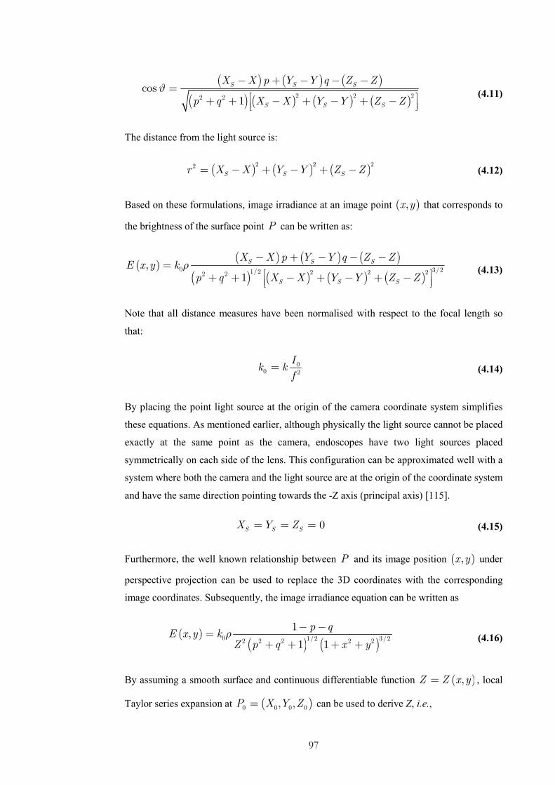
97
( ) ( ) ( )
( ) ( ) ( ) ( )2 2 22 2cos
1
S S S
S S S
X X p Y Y q Z Z
p q X X Y Y Z Zϑ
− + − − −=
+ + − + − + −
(4.11)
The distance from the light source is:
( ) ( ) ( )2 2 22S S Sr X X Y Y Z Z= − + − + − (4.12)
Based on these formulations, image irradiance at an image point ( ),x y that corresponds to
the brightness of the surface point P can be written as:
( )( ) ( ) ( )
( ) ( ) ( ) ( )0 3/21/2 2 2 22 2
,1
S S S
S S S
X X p Y Y q Z ZE x y k
p q X X Y Y Z Zρ
− + − − −=
+ + − + − + −
(4.13)
Note that all distance measures have been normalised with respect to the focal length so
that:
00 2
Ik k
f= (4.14)
By placing the point light source at the origin of the camera coordinate system simplifies
these equations. As mentioned earlier, although physically the light source cannot be placed
exactly at the same point as the camera, endoscopes have two light sources placed
symmetrically on each side of the lens. This configuration can be approximated well with a
system where both the camera and the light source are at the origin of the coordinate system
and have the same direction pointing towards the -Z axis (principal axis) [115].
0S S SX Y Z= = = (4.15)
Furthermore, the well known relationship between P and its image position ( ),x y under
perspective projection can be used to replace the 3D coordinates with the corresponding
image coordinates. Subsequently, the image irradiance equation can be written as
( )( ) ( )0 1/2 3/22 2 2 2 2
1,
1 1
p qE x y k
Z p q x yρ
− −=
+ + + + (4.16)
By assuming a smooth surface and continuous differentiable function ( ),Z Z x y= , local
Taylor series expansion at ( )0 0 0 0, ,P X Y Z= can be used to derive Z, i.e.,

98
( ) ( )0 0 0Z Z X X Z X Y Y Z Y= + − ∂ ∂ + − ∂ ∂ + (4.17)
By omitting the higher order terms, we have:
( ) ( )0 0 0 0 0Z Z X X p Y Y q= + − + − (4.18)
where the components of the normal vector [ ]0 0, , 1p q − at the surface point 0P are given
by:
0 00 ,|X X Y Y
Zp
X= =
∂=∂
and 0 00 ,|X X Y Y
Zq
Y= =
∂=∂
(4.19)
Function Z can also be represented in terms of the image coordinates by taken into
account the perspective projection, which yields
( )0 0 0 0 0
0 0
1
1
Z p x q yZ
p x q y
− −=
− − (4.20)
The substitution of the above expression into the image irradiance equation results in the
following formulation:
( )( )
( ) ( ) ( )
3
0 00 1/2 3/222 2 2 2 2
0 0 0 0 0 0 0
1,
1 1 1av
p x q yE x y k
Z p x q y p q x yρ
− −=
− − + + + + (4.21)
This equation represents image irradiance corresponding to a planar patch approximation of
the surface around [ ]0 0 0 0 0 0, ,P x Z y Z Z= . In Equation (4.56), avρ represents the average
albedo in the neighbourhood of 0P , and it is evident that the above image irradiance
equation is a non-linear function of 0p , 0q , 0Z and avρ .
Further information about the local analysis of image irradiance is obtained from the
directional derivatives. The variation of image irradiance along the x and y directions can
be obtained by using the partial derivatives of the image intensity , i.e.,
E EdE dx dy
x y
∂ ∂= +
∂ ∂ (4.22)
By differentiating the image irradiance equation with respect to x and y , we have:

99
0 0 0 02 2
0 0 0 0 0 0
31 1
dE p dx q dy x dx y dy
E p x q y x y
+ + = − + − − + + (4.23)
There are two important outcomes from this formulation. Firstly, the derivative of the
image irradiance equation is proportional to the image intensity itself. Secondly, the
average albedo avρ and the camera constant 0k have been cancelled out. Subsequently, the
surface information encoded in the normal components ( )0 0,p q depends only on image
intensities and the image coordinate position of the correspondent pixel. Since dx and dy
are in two independent directions, the x and y components of the normalised derivatives
can be separated. Therefore, after some algebraic manipulations, a system of two linear
equations with the two unknowns can be derived:
1 0 1 0 1
2 0 2 0 2
0
0
A p B q C
A p B q C
⋅ + ⋅ + = ⋅ + ⋅ + = (4.24)
where
( ) ( )( )( )
( )( ) ( )
( )
2 2 21 0 0 0 0
2 21 0 0 0 0 0
2 21 0 0 0
2 22 0 0 0 0 0
2 2 22 0 0 0 0
2 22 0 0 0
3 1 3
1 3
1 3
1 3
3 1 3
1 3
x
x
x
y
y
y
A x R x y x
B R x y y x y
C R x y x
A R x y x x y
B y R x y y
C R x y y
= − ⋅ + ⋅ + + − ⋅ = − ⋅ + + ⋅ − ⋅ ⋅ = ⋅ + + + ⋅ = − ⋅ + + ⋅ − ⋅ ⋅ = − ⋅ + ⋅ + + − ⋅ = ⋅ + + + ⋅
(4.25)
In the above equation, x xR E E= and y yR E E= are the normalized partial
derivatives of the image intensities, E is the intensity of the pixel under consideration and
0x and 0y are the normalized image plane coordinates. In practice, the partial derivatives
involved in the above equations can be estimated by convolving the image with a 3×3
Sobel kernel.
To demonstrate how the above algorithm works, Figure 4.2 demonstrates the derived pq-
distribution from in vivo bronchoscopic images. These values can be integrated to form a
3D surface representation of the airways, as shown in Figure 4.2, where the reconstruction
was based on the algorithm proposed by Agrawal et al [134]. This technique uses graph
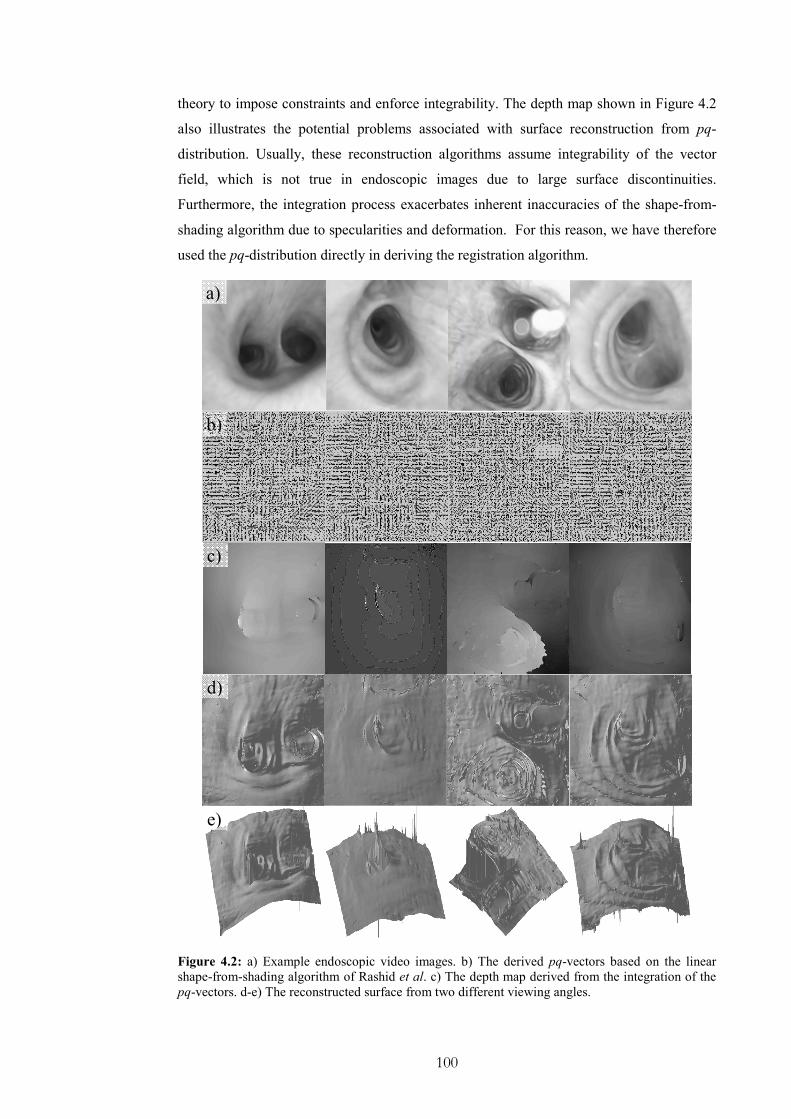
100
theory to impose constraints and enforce integrability. The depth map shown in Figure 4.2
also illustrates the potential problems associated with surface reconstruction from pq-
distribution. Usually, these reconstruction algorithms assume integrability of the vector
field, which is not true in endoscopic images due to large surface discontinuities.
Furthermore, the integration process exacerbates inherent inaccuracies of the shape-from-
shading algorithm due to specularities and deformation. For this reason, we have therefore
used the pq-distribution directly in deriving the registration algorithm.
Figure 4.2: a) Example endoscopic video images. b) The derived pq-vectors based on the linear
shape-from-shading algorithm of Rashid et al. c) The depth map derived from the integration of the
pq-vectors. d-e) The reconstructed surface from two different viewing angles.
a)
b)
c)
d)
e)

101
4.3.2 Extraction of pq-components from the 3D Model
-0.4
-0.3
-0.2
-0.1
0
0.1
0.2
0.3
0.4
Figure 4.3: a) A rendered pose of the 3D model and b-c) the corresponding p, q components,
respectively. The p, q components have been derived by differentiating the z-buffer and the
colormap encodes the value of p and q for each pixel.
As for tomographic images, the extraction of the pq components from the 3D model is
relatively straightforward as the exact surface representation is known. Differentiation of
the z-buffer for the rendered 3D surface will result in the required pq distribution, which
also elegantly avoids the tasks of occlusion detection. The effect of perspective projection
has been taken into account during the rendering stage. An example of the extraction of the
pq-components from the z-buffer is shown in Figure 4.3.
p z x= ∂ ∂ , q z y= ∂ ∂ (4.26)
4.3.3 Similarity Measure
At a first glance, one would expect to use the angle ϑ between the surface normals
extracted from shape-from-shading and those from the 3D model for constructing a
minimization problem for 2D/3D registration, i.e.,
( )( )3 3
2 2 2 23 3
1
1 1
img D img D
img img D D
p p q q
p q p qϑ
+ +=
+ + + + (4.27)
This, however, was proved ineffective because of the scaling problems and image noise
involved. We used instead the pq components directly to formulate the similarity measure.
a) b) c)

102
Analytically, for each pixel of the video frame, a pq-vector corresponding to the normalised
surface normal, ( ) , ,, ,T
img i j i jn i j p q = , was calculated by using the linear shape-from-
shading algorithm described above. Similarly, for the current pose of the rendered 3D
model, the corresponding pq-vectors ( )3 , ,, ,T
D i j i jn i j p q ′ ′= for all rendered pixels also
extracted by differentiating the z-buffer. The similarity of the two images was determined
by evaluating the dot product of corresponding pq-vectors as
( ) ( )( )( ) ( )
( ) ( )3
3
3
, ,, , ,
, ,
D img
D img
D img
n i j n i jn i j n i j
n i j n i jϕ
⋅=
⋅ (4.28)
By introducing a weighting factor that is proportional to the norm of 3Dn , the above
equation can be reduced to:
( ) ( )( )( ) ( )
( )3
3
, ,, , ,
,
D img
w D img
img
n i j n i jn i j n i j
n i jϕ
⋅= (4.29)
In practice, the weight needs to be normalised to reduce the effect of spurious data due to
noise amplified by the differentiation of the z-buffer. This is also necessary to avoid the
degeneration of the similarity measure and the introduction of local minima. This problem
is caused by low values of the pq components, such as when the camera directly faces the
tracheo-bronchial wall. The normalised similarity measure can be represented as:
( ) ( )( )( ) ( )
( ) ( )
( )3 3
333
, , ,, , ,
, ,
D img D
w D img
DD img
n i j n i j n i jn i j n i j
Nn i j n i jϕ ′
⋅= (4.30)
where 3DN is the average length of the pq vectors derived from the 3D model. In this
formulation, the pq vectors are also normalised, ( )3 ,D normn i j , based on an empirically
chosen upper limit K .
( )( )
3
3
3,
,
,
D normD
D normi j
n i jN
n i j K=∑
(4.31)
By incorporating the mean angular differences and the associated standard deviations σ, the
following similarity function can be derived:

103
( ) ( )( )3Dw wS Nϕ σ ϕ′ ′= ⋅ ⋅∑ ∑ (4.32)
To formulate a minimisation problem, the above similarity measure takes the form as
shown below:
( ) ( )( )3
1
1 Dw w
S
Nϕ σ ϕ′ ′
=⋅ − ⋅∑∑ ∑∑
(4.33)
By minimising the above equation, the optimal pose of the camera for the video image can
be derived. The reason for introducing a weighting factor is due to the fact that pq-
estimation from the 3D model is more accurate than that of the shape-from-shading
algorithm. This is because it is not affected by surface textures, illumination conditions or
surface reflective properties The weighting factor therefore reduces the potential impact of
erroneous pq-values from the shape-from-shading algorithm and improves the overall
robustness of the registration process. The standard deviation has been introduced to
increase the specificity of the algorithm based on the premise that a systematic error may
not always indicate pose misalignment. On the contrary, it may be due to inherent
inaccuracies of the pq estimation technique. Based on the standard deviation, poses that
introduce mis-alignment between the image and model pq-vectors are penalised.
Figure 4.4 demonstrates the effect of the normalised weighting factor on the optimisation
landscape. In this figure, the origin corresponds to the optimal pose based on visual
inspection and manual refinement. By evaluating the similarity measure in a square area
around this pose, the shape of the function to be optimised is revealed. The white square
indicates where the minimum is located. The weighting factor bounds the minimum in an
area that is close to the optimal position. Without the use of this factor, the similarity
measure can easily slide to a minimum introduced by texture discrepancies.
Ideally, the optimisation landscape should be smooth and free of local minima. For the pq-
based registration approach, this landscape depends also on the distinctive features of the
endoscope image. Bifurcations tend to be the best example of optimisation landscape due to
the uniqueness of the geometrical feature, whereas frames acquired when the camera faces
the lumen exhibit a poor global minimum.

104
Figure 4.4: Examples demonstrating the effectiveness of the normalised weighting factor. On the
left column is the similarity measure with the normalised weighting factor. On the right column is
the similarity measure based on the angle. The position at (0,0) coordinates corresponds to the
optimal pose based on visual inspection and manual refinement. By evaluating the similarity
measure in a square area around this pose, the shape of the function to be optimised is revealed. The
white square indicates where the minimum lie.
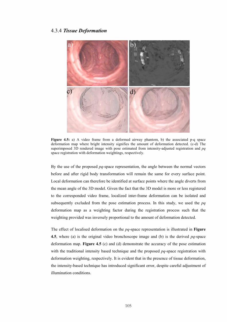
105
4.3.4 Tissue Deformation
Figure 4.5: a) A video frame from a deformed airway phantom, b) the associated p-q space
deformation map where bright intensity signifies the amount of deformation detected. (c-d) The
superimposed 3D rendered image with pose estimated from intensity-adjusted registration and pq
space registration with deformation weightings, respectively.
By the use of the proposed pq-space representation, the angle between the normal vectors
before and after rigid body transformation will remain the same for every surface point.
Local deformation can therefore be identified at surface points where the angle diverts from
the mean angle of the 3D model. Given the fact that the 3D model is more or less registered
to the corresponded video frame, localized inter-frame deformation can be isolated and
subsequently excluded from the pose estimation process. In this study, we used the pq
deformation map as a weighting factor during the registration process such that the
weighting provided was inversely proportional to the amount of deformation detected.
The effect of localised deformation on the pq-space representation is illustrated in Figure
4.5, where (a) is the original video bronchoscope image and (b) is the derived pq-space
deformation map. Figure 4.5 (c) and (d) demonstrate the accuracy of the pose estimation
with the traditional intensity based technique and the proposed pq-space registration with
deformation weighting, respectively. It is evident that in the presence of tissue deformation,
the intensity-based technique has introduced significant error, despite careful adjustment of
illumination conditions.

106
4.3.5 Video Preprocessing
Figure 4.6: The pre-processing steps applied to the bronchoscope videos before 2D/3D registration.
a) Original video frame acquired from the prototype bronchoscope, b) de-interlaced video frame, c)
after lens distortion correction, and d) final smoothed image by using an anisotropic filter that
preserves local geometrical features.
Pre-processing of the videos was necessary in order to alleviate the effects of interlacing,
lens distortion and filter out redundant texture information. In Figure 4.6 the main steps
involved in video pre-processing are illustrated, which include de-interlacing, distortion
correction, and anisotropic filtering.
Digital camcorders and VCRs that use either NTSC or PAL format interlace two
consecutive frames into one such that one video frame contains the even and the next the
odd lines. We used VirtualDub filter (http://biphome.spray.se/gunnart/video/) to remove
interlacing. Furthermore, the wide angle lens of the bronchoscope camera can cause severe
barrel distortions. In general, methods that correct for ‘barrel’ distortion must calculate the
centre of distortion and correct for both radial and tangential components. Radial distortion
is the most commonly seen distortion and it causes the actual image plane to be displaced
radially in the image plane. Tangential distortion is due to ‘decentering’ or imperfect
centring of the lens or other manufacturing defects. For camera calibration, we used the
107
OpenCV matlab toolbox, which includes both radial and tangential distortion correction
steps.
The initialization of the calibration parameters is similar to Zhang et al. [135] based on a
closed-form solution after distortion correction. The intrinsic parameters of the camera have
been estimated along with the first five coefficients that characterise the distortion of the
lens. Subsequently, the distortion parameters are used to restore each endoscopic frame,
and the intrinsic camera parameters are used to derive the perspective projection. The
mathematical details involved in this step are provided in Appendix A. Finally, a structure
adaptive anisotropic filter was applied to the video image to remove image noise and
artefacts [136]. The method uses a local orientation and an anisotropic measure of level
contours to control the shape and extent of the filter kernel, and thus ensures that corners
and edges are well preserved through out the filtering process.
4.4 Experiments and Results
The proposed method was implemented in Microsoft Visual C++ on a conventional PC
machine (2 GHz Intel Pentium 4 processor, 512MByte main memory, nVidia GeForce 4
MX 440 graphics card, with Microsoft Windows 2000 operating system). Surface rendering
was implemented using OpenGL. The interface was based on FLTK (www.fltk.org). The
technique has been validated both with phantom data and in vivo data. For the phantom
validation ground truth data are acquired from a 6DoF EM tracker attached to the camera.
For the in vivo study ground truth data has been collected by manually registering selected
poses and interpolating the intermediate points.
4.4.1 Phantom Study
In order to assess the accuracy of the proposed algorithm, an airway phantom made of
silicone rubber and painted with acrylics, as shown in Figure 4.7 (a), was constructed. The
phantom has a cross sectional diameter of 12cm at the opening and narrows down to 5cm at
the far end. The inside face was coated with silicone-rubber mixed with acrylic for surface
texturing and left to cure in the open air. This gives the surface a specular finish that looks
similar to the surface of the lumen. A real-time, six degrees-of-freedom Electro-Magnetic

108
(EM) motion tracker (FASTRAK, Polhemus), shown in Figure 4.7 (b), was used to validate
the 3D camera position and orientation. The EM-tracker has an accuracy of 0.762mm RMS.
The tomographic model of the phantom was scanned with a Siemens Somaton Volume
Zoom four-channel multi-detector CT scanner with a slice thickness of 3mm and in-plane
resolution of 1mm. A CMOS camera and NTSC standard with frame rate of 29.97fps was
used.
Figure 4.7: a) An airway phantom made of silicon rubber and painted with acrylics was constructed
in order to assess the accuracy of the pq-based registration. b) A real-time six DOF EM tracker
motion tracker (FASTRAK, Polhemus) was used to validate the 3D camera position and orientation.
a)
b)

109
4.4.2 In vivo Validation
a)
b)
Figure 4.8: Assessment of manual alignment error compared to the EM tracker as assessed by
using the 3D bronchial model. a) Euclidean distance between the first and subsequent camera
positions as measured by the EM tracker and after manual alignment with step equal to 10. b) Inter-
frame angular difference between manual alignment and readings from the EM tracker.
For preliminary in vivo validation, bronchoscopy examination was performed in one patient
according to a conventional clinical protocol. During the bronchoscope procedure a
prototype videoscope (Olympus BF Type; with field of view 120°) was used. Video images
from the bronchoscopic examination were transferred to digital videotapes in PAL format
at 25fps. Since the original endoscopic video frames contain both the endoscopic image and
redundant black background, only the endoscopic view was digitised and cropped to
images of 454×487 pixels. All images were converted to greyscale before the pq-space

110
analysis. Similar to the phantom study, the CT images were acquired from the Siemens
Somaton Volume Zoom four-channel multi-detector CT scanner with a slice width of 3mm
and collimation of 1mm, and the acquisition volume covered from the aortic arch to the
dome of hemi-diaphragm.
The technique has been evaluated both with qualitative and quantitative analyses.
Quantitative results were obtained with gold standard data derived from manual alignment
of the 3D model to the video frames. Manual alignment always entails an error. To assess
this, the distance from the initial reference position and the angle from the initial vector are
displayed in Figure 4.8 for both the EM tracking data and the manual alignment. The
measurements have been done by using the airway phantom and the EM tracker. Analogous
to phantom validation, a video sequence has been tracked for more than 400 frames using
the EM tracker. For the same sequence we used manual alignment for every 10frames to
get the position of the virtual camera that matches best the corresponding video view. The
average positional error is equal to 3mm with STD 2.26mm and the angular error is
0.0381rad with STD 0.0285rad. This indicates that the error is consistent throughout the
video sequence and relatively small. We expect that this error will be smaller in real
bronchoscope images as the phantom’s scale is greater than the real size of the airways.
4.5 Results
4.5.1 Phantom study
To assess the accuracy of the proposed algorithm in tracking camera poses in 3D, Figure
4.9 and Figure 4.10 compare the relative performance of the traditional intensity based
technique and EM tracked poses against those from the new method. Since the tracked pose
has six degrees-of-freedom, we used the distance travelled and inter-frame angular
difference as a means of error assessment. The video acquired has 1.73 minutes duration
(25fps). A continuous part of 40 sec (1000 frames) has been used for tracking. Traditional
cross-correlation with the illumination conditions manually adjusted failed when the
bronchoscope gets through the main bifurcation to the left bronchi and faces directly the far
end of the tubular phantom airway, (394 frame). Three different variations of the pq-space
technique were tested and compared against the gold standard EM tracker data (black line)
and the intensity based technique (blue line). As expected the intensity-based technique is
highly sensitive to lighting condition changes, and with manual intensity adjustments, the

111
convergence of this method is improved. However, the proposed pq-space registration has
significantly consistent results, which were close to those measured by the EM tracker. It is
also evident that the weighting factor affects greatly the performance of the method and can
enhance significantly its accuracy. By choosing a weight related to the z-buffer variations,
errors caused by variations in texture and surface reflection can be minimised.
Figure 4.9: Euclidean distance between the first and subsequent camera positions as measured by
four different tracking techniques corresponding to the conventional intensity based 2D/3D
registration with or without manual lighting adjustment, the EM tracker and the proposed pq space
registration technique.
Figure 4.10: Inter-frame angular difference at different time of the video sequence, as measured by
the four techniques described in the above figure.

112
Figure 4.11: In vivo validation results for a patient study. The left column shows examples of real
bronchoscopic images. The right column presents the virtual bronchoscopic images after pq-space
based 2D/3D registration.
4.5.2 In vivo validation
Qualitative results from the in vivo validation are demonstrated in Figure 4.11, where
sample frames from the video sequence are displayed. The proposed pq-space based
registration has been applied to a video sequence of 31sec (797 frames) of the one-patient
study. The bronchoscope video sequence starts from the main bifurcation and continues
through the left bronchi. Visual inspection of the real and the virtual endoscope images
proves that the pq-based registration technique can track the tip of the bronchoscope
relatively accurately and is stable under sudden movements or large rotation angles.
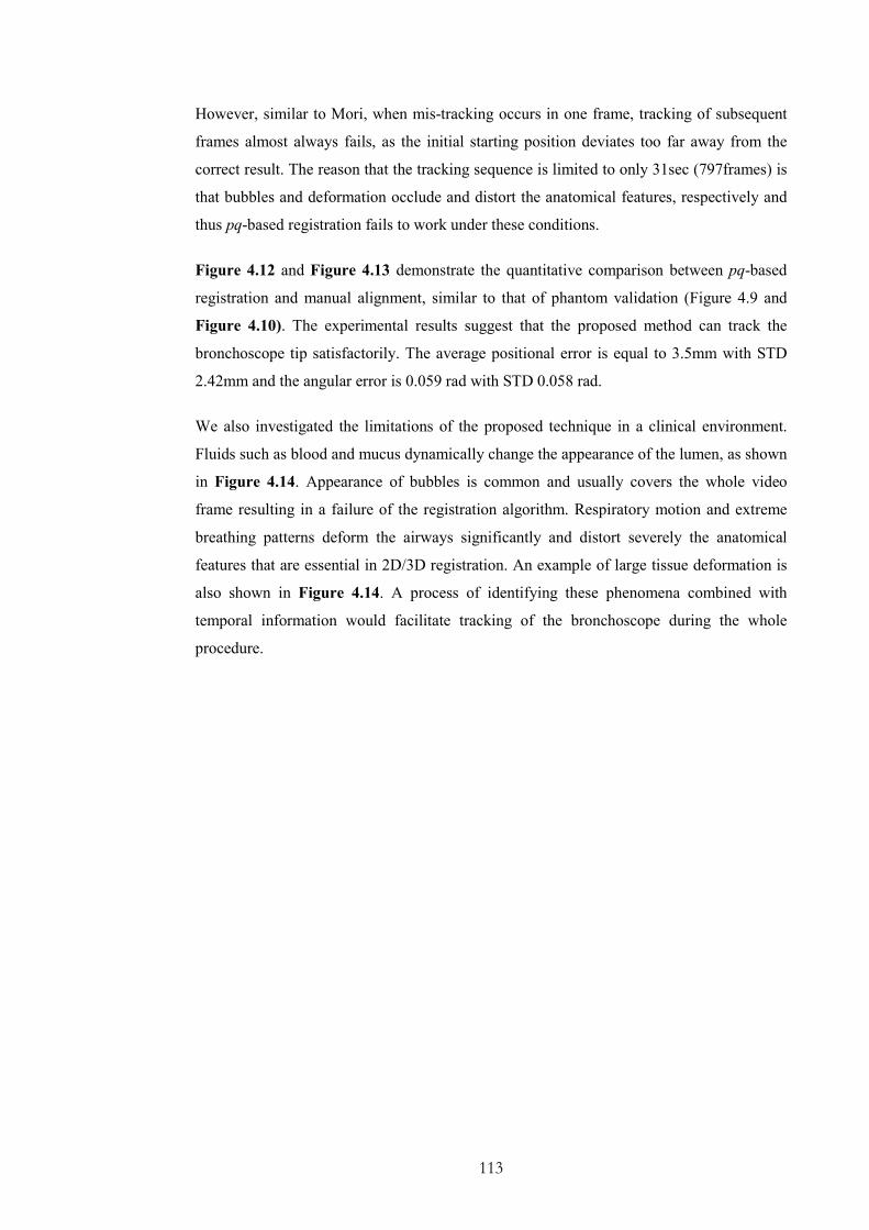
113
However, similar to Mori, when mis-tracking occurs in one frame, tracking of subsequent
frames almost always fails, as the initial starting position deviates too far away from the
correct result. The reason that the tracking sequence is limited to only 31sec (797frames) is
that bubbles and deformation occlude and distort the anatomical features, respectively and
thus pq-based registration fails to work under these conditions.
Figure 4.12 and Figure 4.13 demonstrate the quantitative comparison between pq-based
registration and manual alignment, similar to that of phantom validation (Figure 4.9 and
Figure 4.10). The experimental results suggest that the proposed method can track the
bronchoscope tip satisfactorily. The average positional error is equal to 3.5mm with STD
2.42mm and the angular error is 0.059 rad with STD 0.058 rad.
We also investigated the limitations of the proposed technique in a clinical environment.
Fluids such as blood and mucus dynamically change the appearance of the lumen, as shown
in Figure 4.14. Appearance of bubbles is common and usually covers the whole video
frame resulting in a failure of the registration algorithm. Respiratory motion and extreme
breathing patterns deform the airways significantly and distort severely the anatomical
features that are essential in 2D/3D registration. An example of large tissue deformation is
also shown in Figure 4.14. A process of identifying these phenomena combined with
temporal information would facilitate tracking of the bronchoscope during the whole
procedure.

114
Figure 4.12: In vivo validation: Euclidean distance between the first and subsequent camera
positions as measured by the pq-based 2D/3D registration and from manual alignment for ten
random frames of the sequence.
Figure 4.13: In vivo validation: Inter-frame angular difference at different time of the video
sequence, as measured by the two techniques described in Figure 4.12.
Figure 4.14: Common image artefact that can affect image-based 2D/3D registration techniques: a)
excessive bleeding due to pathology, b) appearance of bubbles when patient coughs, and c-d) large
tissue deformation between successive image frames.

115
4.6 Discussions and Conclusions
In this chapter, we have proposed a new pq-space based 2D/3D registration method for
recovering camera poses of bronchoscope videos. The results indicate that based on the pq-
space and the 3D model, reliable bronchoscope tracking can be achieved. One major
advantage of the method is that it is not affected by illumination conditions. This is a
condition that the traditional intensity-based techniques fail due to dynamic changes in the
overall illumination parameters when the bronchoscope passes through the main bifurcation
to the bronchi. The pq-space based technique is less sensitive to these changes and it does
not require the extraction and matching of explicit feature vectors.
However, pq-based registration can be influenced by the surface texture of the endoscopic
images. For this reason a weighting factor has been incorporated into the similarity
measure. This factor is estimated from the salient features that are present in both the
projected images of the 3D model as well as those that appear in the endoscopic video. In
this way, erroneous surface normals due to noise and texture discrepancies are ignored.
Phantom as well as in vivo validation has shown that the similarity measure is robust and
resilient to variations of surface texture details.
Another important implication of the incorporation of surface normals in the registration
scheme is the ability to identify airway deformation between successive image frames.
Preliminary results indicate that deformation of the airways can be identified and excluded
from the registration process. However, in doing so we have assumed that the
bronchoscope moves smoothly through the airways and the deformation is only limited to a
small part of the video frame. Further investigation of the accuracy of the method for large
tissue deformation is required. To this end, explicit airway deformation modelling may
become necessary.
It should also be noted that there are a number of factors that can affect the accuracy of the
pq-space algorithm. The 3D reconstruction of the tracheo-bronchial tree can involve
artefacts due to respiratory motion and partial volume effects. Since the respiratory status
during imaging and that during video bronchoscope examination are not matched, the 3D
airway anatomy can differ significantly from the dynamic appearance of the tracheo-
bronchial tree during the examination. Furthermore, bronchoscope cameras typically have a
wide angle coverage, which can also cause adverse effects on the accuracy of pq-space
estimation despite the use of distortion correction.
116
With the proposed method, the intrinsic robustness of the technique is dependent on the
performance of the shape-from-shading method used. The use of camera/lighting
constraints of the bronchoscope greatly simplifies the 3D pose estimation of the camera.
Nevertheless, it is important to note that shape-from-shading is also affected by
specularities and inter-reflectance caused by mucus and the lumen surface. A number of
improvements need to be introduced for further enhancement of the accuracy of the
proposed framework by explicit incorporation of the effect of mutual illumination, inter-
reflectance and the specular components.
Overall, the most severe artefacts encountered in bronchoscopy are due to bleeding,
mucosa, and large deformation of the tracheo-bronchial tree. In these cases, it is necessary
to introduce temporal constraints to stabilise the registration results. In the following
chapter, we will show that temporal information can be utilised through a probabilistic
framework. Another means of enhancing the robustness of the 2D/3D registration is by
incorporating EM tracking devices, which are capable of real-time tracking of the
bronchoscope tip. As will be discussed later, EM tracking facilitates registration even in the
presence of large tissue deformation and allow for a robust non-rigid registration scheme.
117
Chapter 5
Integration of Temporal Information
ince 2D bronchoscope video only provides localised views of the inner surface of the
lumen, the exact 3D location of the structure it represents is ambiguous. Different
segments of the airways may well have a similar local structure. An example is illustrated
in Figure 5.1, which shows bronchoscope frames from different parts of the tracheo-
bronchial tree. It is evident that the bronchus is a relatively symmetrical structure.
Therefore, visual tracking should not depend only on a frame-by-frame analysis. It should
also consider the path followed by the camera and its motion characteristics. The use of
temporal information to derive the trajectory of the bronchoscope in 3D space is important.
Another advantage of the use of temporal correspondence is that the estimates of the
camera’s orientation and position can be used to accelerate the registration and tracking of
consecutive video frames.
For video bronchoscope navigation, Naga et al [137] used Kalman filtering to exploit
temporal information in order to increase the speed and accuracy of the registration process.
Kalman Filtering was introduced in 1960 by Rudolph Kalman as an optimal linear
estimator. It is a recursive data processing algorithm which makes optimal use of imprecise
data on a linear (or nearly linear) system with Gaussian errors to continuously update the
best estimate of the system's current state. Kalman filter is statistically optimal in that it
minimizes the mean-square error and incorporates all available information to estimate the
current value of the variables of interest. The information used includes (1) knowledge of
the system and measurement device dynamics; (2) the statistical description of the system
noises, measurements errors and uncertainty in the dynamics models; and (3) information
about initial conditions of the variables of interest. In other words, Kalman filter is, in fact,
a learning method. It uses a model of the estimation problem that distinguishes between
S
118
what is observed, what is really going on, and the state of knowledge about the real status
of the system and the one that can be deduced from the observations. That state of
cognition is represented by probability distributions that correspond to knowledge of the
real world.
Kalman filtering is a viable framework for tracking the bronchoscope camera, since it
provides a means of inferring the missing information from indirect and noisy
measurements. However, practical application of Kalman filtering requires careful
consideration of underlying statistical modelling and numerical precision. Typically,
Kalman filtering is based on the assumptions of linearity, white noise and Gaussian noise
[138]. These assumptions cannot always be fulfilled in a real situation. The robustness of
Kalman filtering in practice depends on the extent of these assumptions being violated.
There are methods for extending Kalman filtering to more general cases but usually they
compromise the optimal behaviour of the filter and lead to considerably more complex
systems. Furthermore, these approaches do not take into account all prominent statistical
characteristics of the process under consideration, and hence they often yield poor results.
In bronchoscopy, tissue deformation, inter-reflection, multi-texture background, and view
dependent specularity due to mucosa can limit the accuracy of image-based algorithms.
Kalman filtering does not provide a mechanism to overcome this problem and the
effectiveness of the method has so far been limited. Dis-occlusion is common in
bronchoscopy navigation, since bubbles and luminal fluids can cover partially or
completely a video segment. Although dis-occlusion often lasts only for a few seconds,
during this time, the position of the bronchoscope camera can be moved significantly.
Without temporal tracking, the current techniques can only work for relatively short
segments. Furthermore, the potential artefacts described above can result in a multi-modal
distribution of the probability density function of the state vector. Therefore, the
observation probabilistic model cannot be approximated as a Gaussian distribution. It is
also important to note that the assumptions of linearity and whiteness may be also violated
in bronchoscope tracking.
To circumvent the above problems, we aim to develop in this thesis a predictive tracking-
algorithm to propagate the probability distribution of the state space based on the
Conditional Density Propagation (Condensation) algorithm [139]. The method is designed
to cater for the general situation when several competing observations forming a non-
Gaussian state-density are encountered. It uses a stochastic approach that has no restriction
on the system/measurement models used and the distribution of error sources. Therefore,
none of the assumptions about linearity, gaussianity and whiteness needs to hold.
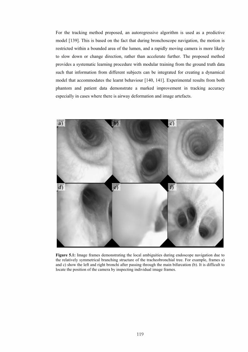
119
For the tracking method proposed, an autoregressive algorithm is used as a predictive
model [139]. This is based on the fact that during bronchoscope navigation, the motion is
restricted within a bounded area of the lumen, and a rapidly moving camera is more likely
to slow down or change direction, rather than accelerate further. The proposed method
provides a systematic learning procedure with modular training from the ground truth data
such that information from different subjects can be integrated for creating a dynamical
model that accommodates the learnt behaviour [140, 141]. Experimental results from both
phantom and patient data demonstrate a marked improvement in tracking accuracy
especially in cases where there is airway deformation and image artefacts.
Figure 5.1: Image frames demonstrating the local ambiguities during endoscope navigation due to
the relatively symmetrical branching structure of the tracheobronchial tree. For example, frames a)
and c) show the left and right bronchi after passing through the main bifurcation (b). It is difficult to
locate the position of the camera by inspecting individual image frames.
a) b) c)
d) e) f)

120
5.1 A Probabilistic Framework in Visual Tracking
Most of 2D/3D registration applications use either image-based techniques and/or
incorporate positional information from tracking devices. Both of these approaches have
their limitations in terms of accuracy and computational complexity. Image-based
registration techniques are derived from mathematical models that are not perfect. They
depict only those characteristics of direct interest and under essential simplifications in
terms of lighting conditions and camera modelling. As described in Chapter 4, Lambertian
surface properties and a pinhole camera model are usually assumed, and inter-reflections,
dis-occlusion due to bleeding and mucosa fluids, and deformation are typically ignored.
Image-based registration is also prone to local minima due to ambiguities of the local
structure, such as when the endoscope is very close to the tracheo-bronchial wall. Once the
tracking fails, the registration process cannot be re-initialised automatically and manual
intervention is necessary.
The use of physical tracking devices can potentially solve the problems stated above. The
technique, however, also has certain limitations. For example, accurate mapping of the EM
tracking world coordinate system to the CT coordinate system under deformation is not
trivial, as will be shown in the following chapters. Nevertheless, a probabilistic framework
that combines the measurements of the tracking device and the estimations of the image-
based technique in an optimal fashion is desirable. To provide current estimates of the
system variables a statistical model should be designed to properly weight each new
measurement relative to past information.
The basic concept of a probabilistic tracking framework is summarised in Figure 5.2. The
camera pose is estimated using one or more measurement models. These measurement
models are based either on image features or data provided from tracking devices. These
measurements, also called observations, are inputs to the probabilistic model that
incorporates information about the error both in the prediction and the observations so as to
derive a better estimation of the pose for the next image frame. The prediction model is the
combination of two components: (1) a mathematical model that approximates the camera
motion based on previous measurements; and (2) an uncertainty term that accounts for the
inherent incapacity of such a model to describe, for example, the unknown and the inherent
inaccuracy of the model. The parameters related to the prediction/state model and the
observations uncertainty are estimated or approximated prior to the actual tracking process,
either with a systematic training approach or performed empirically when the motion is
simple to describe.

121
Observation uncertainty factors can also be updated on-line, according to how close the
predicted pose is to the actual measurements. System observability also plays an important
role in system analysis and parameter estimation [142]. It relates to the amount of
information contained in the measurement about the state of the system, and decides
whether the system state is recoverable from the measurements. In other words, if the
system is not observable, its state cannot be completely determined from the measurements,
and additional or alternative measurements should be considered. This can be used as an
evaluation metric of the 2D/3D registration performance.
In summary, the role of the suggested stochastic framework is to estimate the state of
dynamic systems. For the case of bronchoscopy tracking, this state would most probably be
the position and orientation of the camera during navigation. This state can also encode
other information, such as the speed and acceleration of the camera tip. In general, the
dynamic aspects of a system cannot be estimated precisely. This stochastic framework
allows expression of this partial ignorance using probabilities. Therefore, the state of
dynamic systems with certain types of random behaviour can be approximated using
statistical information. Furthermore, this scheme also has the ability to analyse and evaluate
the performance of its components. This analytical capability allows a system designer to
assign an uncertainty factor to subsystems of an estimation system, and to trade off between
computational complexity and real-time processing to optimize the overall system
performance.
EM TrackingDevices
History
Observed Pose 1
AutoRegressive
Model
Real
Camera
Virtual Camera
Image Based
RegistrationObserved
Pose 2
ProbabilisticModel
PropagatedParticles
OptimalPose
Figure 5.2: A schematic diagram of the proposed framework.

122
5.2 Endoscope Tracking Based on Particle Filtering
In visual tracking, it is generally recognised that designing effective tracking algorithms is
difficult, requiring mechanisms to deal with issues such as weak image features,
background clutter, erratic and discontinuous motion, multiple occluding and deforming
objects. Some of these effects are prominent in endoscope tracking and as a result the
typical assumptions of linearity, gaussianity and whiteness do not hold. Filters based on
Bayesian theory, known as the Condensation algorithm or particle filtering, utilise a more
general approach, without over-simplifying the underlying hypothesis. This method can be
seen as a generalisation of Hidden Markov Models in that it allows a discrete set of states
with probabilistic transitions between states. These approaches are flexible, easy to
implement and parallelisable.
The Condensation algorithm is the extension of a sequential Monte Carlo algorithm for
visual tracking of outlines and features of foreground objects, modelled as curves. It has
been introduced by Isard et al. [143] for developing agile trackers that are immune to
distraction from background clutter. The Condensation algorithm is designed to
accommodate complex posterior distributions, non-linear dynamics and ambiguous image
data [144]. Therefore, it is capable of addressing the more general situation of a non-linear
system with non-Gaussian state distributions. Nevertheless, it is considerably simpler than
the Kalman filter. Despite the use of random sampling which is often thought to be
computationally inefficient, the algorithm can be executed in near real-time. This is because
tracking over time maintains relatively tight distributions for the position of the camera at
successive time-steps, which is the case, given the availability of accurate, learned models
of the camera motion.
The algorithm uses factored sampling to stochastically propagate a non-Gaussian, multi-
modal estimate of the target posterior with a stochastic differential equation model for
camera motion. To deal with non-Gaussian observation distributions, it maintains multiple
hypotheses, particle sample, and automatically focuses more on the most likely ones. The
weight of each particle is represented by the likelihood of that particular state variable. This
likelihood value is determined by comparing the observed data with the measurement data.
Each hypothesis/particle is propagated through a dynamical model of the camera motion.
The random component of the dynamical model leads to increasing uncertainty while the
deterministic component causes the density function to drift bodily.

123
The main stochastic mechanism that constitutes the probabilistic endoscope tracking
framework developed in this thesis can be summarised into the following three steps: (1)
sampling, where N particles from the original set are chosen, with the probability of
selecting each item being proportional to its weight; (2) evolving, where the dynamic
model is applied to the selected particles; and (3) measuring the coefficients based on the
observations, so the weights of the new density are estimated. Since this includes multi-
modal distributions, particle filters can cope effectively with temporarily ambiguous image
support.
The main idea of the statistical framework is to maintain a time-evolving probability
distribution ( )|t tp x Z of the tracker state tx over time t . The a posteriori density
( )|t tp x Z represents knowledge about tx deducible from the observation
history 1, ,t tZ z z= … . The effective prior distribution ( )1|t tp x Z − in the dynamic case
is unknown and therefore cannot be represented with a closed-form solution. The
Condensation algorithm does not explicitly represent the density function. It uses instead
statistical factor sampling, which provides a way of approximating ( )1|t tp x Z − by using a
random number generator for sampling ( )tp x . The sampling technique is based on the
Bayesian theory which states [145]:
( ) ( ) ( )| |p x z p z x p x∝ (5.1)
Bayesian theory allows a prediction model to incorporate inherent knowledge, while
improving its ability to make decisions through the seamless integration of auxiliary
information.
Factored sampling needs to be extended to be applied iteratively to the image sequence.
The process at each time-step is a self-constrained iteration of factored sampling [146]. In
order for the algorithm to run under a constant computational complexity, the sample sets
should be retained at a fixed size N . During statistical factored sampling, a sample set
( ) ( ) 1 , , Ns s… is generated from the prior density ( )tp x , where N is the number of
sample sets (particles). A weight is subsequently assigned to each particle according to the
observation density
( )
( )( )( )( )
1
|
|
n
n
N n
j
p Z x s
p Z x sπ
=
==
=∑ (5.2)

124
The weighted point set is then used as a representation of the posterior density, which is
becoming more accurate as N increases.
Therefore, the procedure is to sample with replacement N times from the set ( ) 1n
ts − ,
choosing an element with probability( )
1n
tπ − . Elements with high weights are more likely to
be chosen several times, leading to identical copies of elements in the new set, while others
with relatively low weights may not be chosen at all. Subsequently, each element chosen
from the new set is subjected to a predictive step, which corresponds to sampling from the
distribution ( )1|t tp x x − . In this way, the sample set ( ) n
ts for the new time-step is
generated but without its weights. Finally, the observation step from factored sampling is
applied, generating weights from the observation density ( )|t tp z x to obtain the sample-
set representation ( ) ( ) ,n n
t ts π of the state density for the new time-step. By evaluating the
moments of the state density, it is possible to extract the current state. As an
observation/measurement model, the pq-space based 2D/3D registration technique
described in the previous chapter has been used.
5.3 Prediction Model for the Bronchoscopic Camera
In the Condensation algorithm, if the prediction model is too simplistic or its parameters
are not tuned properly then it might not be able to represent the dynamics of the system
adequately. In that case, the estimated posterior gradually drifts away from the observation
value, which can result in a zero weighting factor that completely spoils the outcome of the
algorithm. Therefore, it is important to develop a prediction model and a training system
that can model the motion of the endoscopic camera adequately.
In bronchoscope tracking, the estimated pose in the ( )1 tht − frame of a sequence is the
initial pose for the tht frame. In a probabilistic context, this is equivalent to applying a
Gaussian prior distribution to each frame with fixed covariance but whose mean is simply
the estimated pose from the previous frame. When temporal tracking is employed, we could
take the posterior from the ( )1 tht − frame as the prior for the
tht frame rather than fixing
the prior via one constant covariance for all image frames. However, this idea is not
effective for inferencing the motion between successive time-steps, which is reasonable
only when the camera moves slowly and the registration process is accurate. Furthermore,

125
as the posterior at one time-step is regarded as the prior of the next, statistical information
from measurements steadily accumulates. In other words, the pq-space registration results
will have a time-decreasing influence on the estimated pose. An adequate statistical
framework for motion tracking must provide not only a prior for the first frame, but also a
prior for possible motions, in the broad sense of rigid motion. This dynamical prior
distribution should apply between all successive frames. It needs to have a deterministic
part, giving the expected displacement between successive image frames, as well as a
stochastic component to counteract the otherwise unlimited accumulation of information.
For building a dynamical model for tracking the pose of the bronchoscope camera, it is
important that successive positions are tightly constrained. Rather than using only the
global prior distribution ( )p x . A Markov chain model assumption is therefore more
meaningful. A Markovian assumption presumes that the present state of a system can
always be predicted given the previous n states. A Markov analysis looks at a sequence of
events, and analyses the tendency of one event to follow another. In this way, a new
sequence of random but related events can be produced to have properties similar to the
original. A first-order Markov chain model correlates the distribution of the vector state at a
given time with the immediate predecessor only:
( ) ( )1 1 1| |t t t tp x x x p x x− −=… (5.3)
where ( )1|t tp x x − is the conditional distribution, which indicates the probability of tx
given 1tx − . This is an assumption that can greatly simplify the probabilistic model. Note
that a second-order Markov model taking two predecessors into account can also apply.
A simple, isotropic, first-order Gaussian Markov process is defined as:
( ) 2
1 12
1| exp
2t t t tp x x x x
b− −
∝ − − (5.4)
where b is the average root-mean-square step length and ‘isotropic’ has the meaning of
steps equally likely to occur in all directions. This type of motion is known as Brownian
motion. Such a distribution is too random to be useful for modelling of real object motion.
Instead, a constrained Brownian process is adopted. Although, it initially appears to behave
randomly, in the long-term it is limited within a restricted area of a Gaussian envelope.
All these Markov processes belong to a broader family that is called Auto-Regressive
(ARG) processes and they meet some of the requirements of dynamic modelling by
126
simulating the entire family of motions. The first-order ARG processes deal with changes
in position and can impose strong incremental constraints when global constraints are
weak. They allow a global distribution to be chosen in addition to, and independently of,
the local process. Although, they appear to be the simplest available models that can
achieve these properties, they do have certain limitations. A first-order ARG process seems
to model noisy directional motion at a constant average velocity. However, it has an
average direction that is fixed over time and must be known in advance.
Substantial changes in velocity components over time and oscillations are beyond the scope
of the first-order model. This can limit the applicability of the system in a bronchoscopy
application where the respiratory motion results in a periodic movement of the
bronchoscope tip. A second-order dynamical model is a natural extension of a first-order
ARG process and it can give a much improved result, while it has the potential to specify
an ARG process representing a second-order Markov chain. In other words, the state vector
at a given time depends on two previous time-steps, rather than just one as in the first-order
process.
In order to construct a motion model for the endoscope camera that moves freely in the 3D
tracheo-bronchial tree, a second order auto-regressive model is used [139]. This is in
contrast to the ‘constant acceleration’ model used in [137], which effectively implies that
the camera acceleration is expected to be constant during bronchoscope tracking. In this
study, the auto-regressive model takes into account that during bronchoscope navigation,
motion occurs within a bounded area, and a rapidly moving camera is expected to slow
down or change in direction rather than accelerate further [147]. This ensures smooth
navigation of the camera, and with modular training [140], multiple training sets can be
used to obtain a more general model of the motion behavior. For a 2nd-order auto-regressive
model, the following equation can be used:
2
1
t k t k t
k
x A x Bw−=
= +∑ (5.5)
where kA represents the collection of damped harmonic oscillators associated with
vibrational modes and w the white noise with covariance coefficient B .
In Figure 5.3, an example of the application of a first, as well as a second order ARG
model is demonstrated. The first order ARG model fails to follow the position of the
camera even during the phase of training.

127
a) b)
c) d)
Figure 5.3: a-b) Training results based on a first order ARG model. c-d) Training results based on a
second order Autoregressive Model.
5.4 Learning Dynamics of Bronchoscope Navigation
In practice, it is possible to build a tracking model by approximating its general behaviour
to intuitive expectations of the observed motion. Hand-built models are often used when
the prediction model is described by a first-order autoregressive process. However, for the
purpose of bronchoscopy navigation it is difficult to use this approach due to the high-
dimensionality and complex motion involved. Instead, a training sequence (gold standard
data) can be used. Mathematically, learning motion characteristics from a training sequence
is effectively to estimate the coefficients kA , the mean value X , and the random
component B of an autoregressive process that best model the motion in a training
sequence involving camera poses of 1, , Mx x… . The problem can be expressed in terms of
maximising the log likelihood function L over all coefficients [140]. For a second order
autoregressive model this takes the form:
128
( )
( ) ( )
1 1 2
21
2 2 1 13
, , | , , ,
12 log det
2
M
M
t t t
t
L x x A A C X
B x A x Ax M B−− −
=
=
′ ′ ′− − − − −∑
…
(5.6)
where
t tx x X′ = − (5.7)
and
C BBΤ= (5.8)
In general, this in a non-linear problem, because L is quartic in the unknowns, due to the
fact that X is explicitly estimated together with 1A , 2A and B . The non-linearity can be
removed by defining the constant parameter D [140]:
( )1 2D I A A X= − − (5.9)
The values of 1A , 2A , B and D that maximise the likelihood function L can be found by
solving the linear system of equations below [140]:
( )2 1 0 2 1
20 1 00 2 10
21 1 01 2 11
2 0
0
0
R AR AR D M
R AR AR
R AR AR
− − − − = ′ ′ ′− − = ′ ′ ′− − =
(5.10)
The auto-correlation coefficients ,i jR and ,i jR′ can be computed for i, j = 0, 1, 2 as:
3
M
i t i
t
R x −=
=∑ , ,3
MT
i j t i t j
t
R x x− −=
=∑ , , ,
1
2T
i j i j i jR R RRM
′ = −−
(5.11)
Subsequently, 1A , 2A and D are given by:
( )( )( )
( )1
11 12 02 01 11 12 22 21 11 12
11 01 2 21 11
0 2 2 1 12
A R R R R R R R R
A R AR R
D R AR ARM
−− −
−
′ ′ ′ ′ ′ ′ ′ ′= − − ′ ′ ′= − = − − −
(5.12)
129
The mean of the ARG process, on the other hand, is calculated as below, given that
( )1 2I A A− − is not singular.
( ) 1
2 1X A A D−
= − −I (5.13)
Finally, the covariance coefficient B is estimated as a matrix square root of C :
( )00 2 20 1 10 0
1
2TC R AR AR DR
M= − − −
− (5.14)
Note that parameter B , which expresses the stochastic part of the ARG process, cannot be
determined uniquely, but any solution that satisfies C BBΤ= is acceptable.
Another important issue to consider is the dimensionality of the data. For a system with just
one degree-of-freedom, the situation is relatively straightforward, while multi-dimensional
motion is more difficult to describe. A 6-DoF pose estimation problem is easier to handle if
it is described by a two independent 3-DoF tracking problems that model the position and
the orientation of the camera separately. This implies that for each of these systems the
second order equation can be described from different parameters, thus being more flexible
and easier to train. This is illustrated in Figure 5.4, where for three in-vivo datasets the
Euclidean distance is estimated for both a 6DoF ARG model and a 3DoF-3DoF model.
5.4.1 Modular Training
Usually, it is desirable to broaden the dynamical model to include more than a specific
motion. For the purpose of bronchoscope simulation, it is more meaningful to collect
several training sets from the same as well as different operators in order to construct a
more representative dynamic model. In this case, the problem becomes how to combine
multiple training sets in order to gain knowledge of a more general behaviour. Modular
learning cannot be addressed by simply concatenating the different training sets and then
treating them as one because the abrupt transition between different data sets would be
interpreted as an actual behaviour of the system [139]. To this end, the auto-correlation
coefficients of each training set can be calculated individually and then combined in a
linear fashion. This is similar to the multi-variate algorithm that Reynard et al. [148] and
Wildenberg et al. [140] have used for motion tracking over classes of objects with variable
mean shapes and positions.

130
a) b)
c) d)
e) f)
Figure 5.4: (a,c,e) Training results based on a 6DoF, second order Autoregressive Model. (b,d,f)
Training results based on two simultaneously second order Autoregressive Models of tracking the
position and the orientation of the camera separately.
In the work presented by Wildenberg et al. [140], modular learning is also based on the
maximum likelihood estimation to find the best model that fits all the training sequences.
The extension of the training algorithm for a single to multiple training sets is presented in
Blake et al. [139] and it is straightforward when the mean of the state vector, X , is
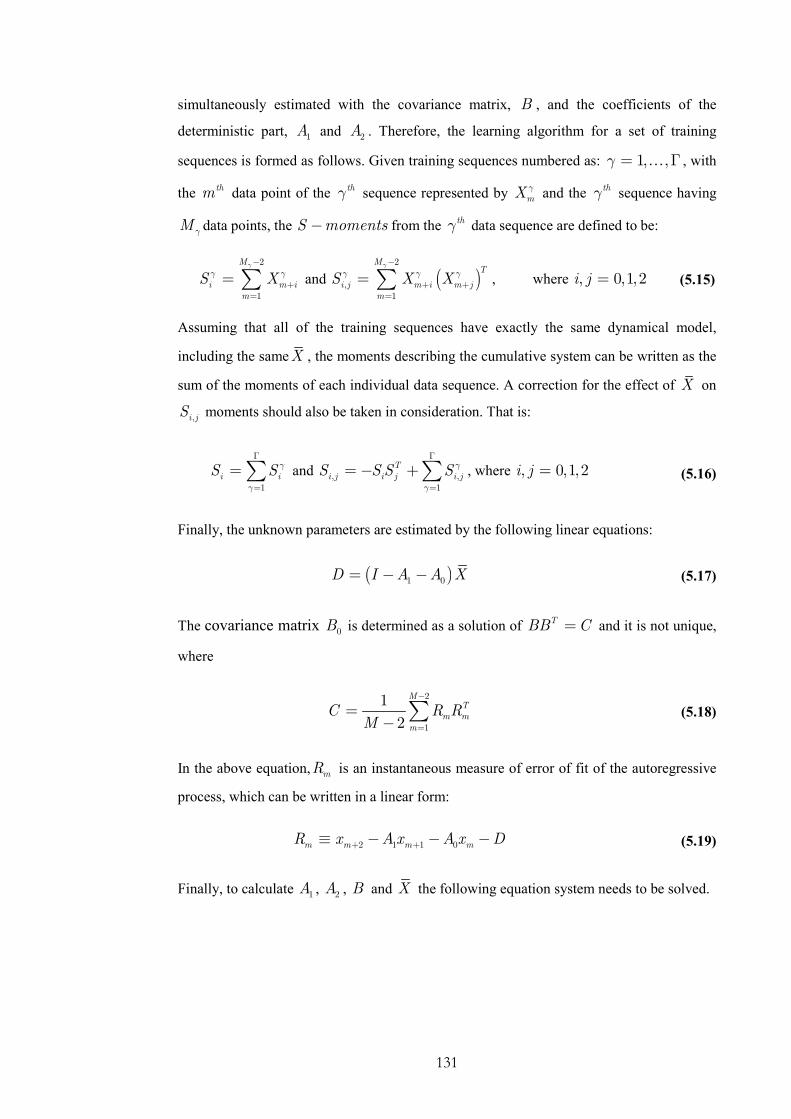
131
simultaneously estimated with the covariance matrix, B , and the coefficients of the
deterministic part, 1A and 2A . Therefore, the learning algorithm for a set of training
sequences is formed as follows. Given training sequences numbered as: 1, ,γ = Γ… , with
the thm data point of the
thγ sequence represented by mXγ and the
thγ sequence having
M γ data points, the S moments− from the thγ data sequence are defined to be:
2
1
M
i m i
m
S Xγ
γ γ
−
+=
= ∑ and ( )2
,1
MT
i j m i m j
m
S X Xγ
γ γ γ
−
+ +=
= ∑ , where , 0,1,2i j = (5.15)
Assuming that all of the training sequences have exactly the same dynamical model,
including the sameX , the moments describing the cumulative system can be written as the
sum of the moments of each individual data sequence. A correction for the effect of X on
,i jS moments should also be taken in consideration. That is:
1i iS S γ
γ
Γ
=
=∑ and , ,1
T
i j i j i jS S S S γ
γ
Γ
=
=− +∑ , where , 0,1,2i j = (5.16)
Finally, the unknown parameters are estimated by the following linear equations:
( )1 0D I A A X= − − (5.17)
The covariance matrix 0B is determined as a solution of TBB C= and it is not unique,
where
2
1
1
2
MT
m m
m
C R RM
−
=
=− ∑ (5.18)
In the above equation, mR is an instantaneous measure of error of fit of the autoregressive
process, which can be written in a linear form:
2 1 1 0m m m mR x Ax A x D+ +≡ − − − (5.19)
Finally, to calculate 1A , 2A , B and X the following equation system needs to be solved.

132
( )2 0 0 1 1
2,0 0 0,0 1 1,0
2,1 0 0,1 1 1,1
2 0
0
0
S A S AS D N
S A S AS
S A S AS
− − − − = − − = − − =
(5.20)
a) b)
c) d) Figure 5.5: Four sequences of the camera position during in vivo navigation have been used for
modular training. These have been extracted from four different subjects. This figure presents the
Euclidean distance from an initial reference point of each of these training sequences.
5.4.2 Model Dynamic Variability
In the work presented by Wildenberg et al., it is also noted that the mean of the sequence is
not the mean of the system. However, the mean of the sequence are often used as a good
estimation when the training data are stable over a long time period:
1
1lim
N
iN i
X XN→∞ =
=∑ (5.21)

133
Nonetheless, if the training sequence is short and weakly damped there is a systematic error
in X . It can cause the rest of the terms to be falsely estimated. In practice, the numerical
error can be large enough to change the overall characteristics of the system, causing
erroneous damped behaviour and shifts of the phase and the frequency. This is profound
when several training sequences are employed. Since each of these dynamic systems may
have a different mean value, the use of pre-estimated mean value of the system can result in
a strongly biased prediction. Alternatively, X can be estimated on-line as part of the state
vector. In this way, the state vector is extended by regarding X as a variable, rather than a
constant [140, 148]. Hence the prediction model can be written as:
1
2 0 1 0 1 1 0
2 1
0 0 0
00 0
n n
n n n
n n
IX X
X A A I A A X B w
IX X
+
+ +
+ +
= − − ⋅ +
(5.22)
Here X is not known as a priori but it is updated during tracking, and X is initialized
with its estimated mean value 0X and its associated variance and covariance.
The ground truth data of the camera pose from four different patients have been used to
train the auto-regressive model. This data are displayed in Figure 5.5. Figure 5.6 illustrates
the effectiveness of the training process involved in this study. The performance of the
trained model was evaluated on a different subject. The Euclidean distance between the
first and subsequent camera positions predicted from the Condensation algorithm was used
for error analysis. Similar analysis for the error in orientation was also performed. In Figure
5.6 (a), the system mean has been predefined according to the training sequences, whereas
for (b), it was included in the state vector of the predictive model such that it was updated
in real-time. It is evident that without continuous updating of X , the derived tracking value
is heavily biased.
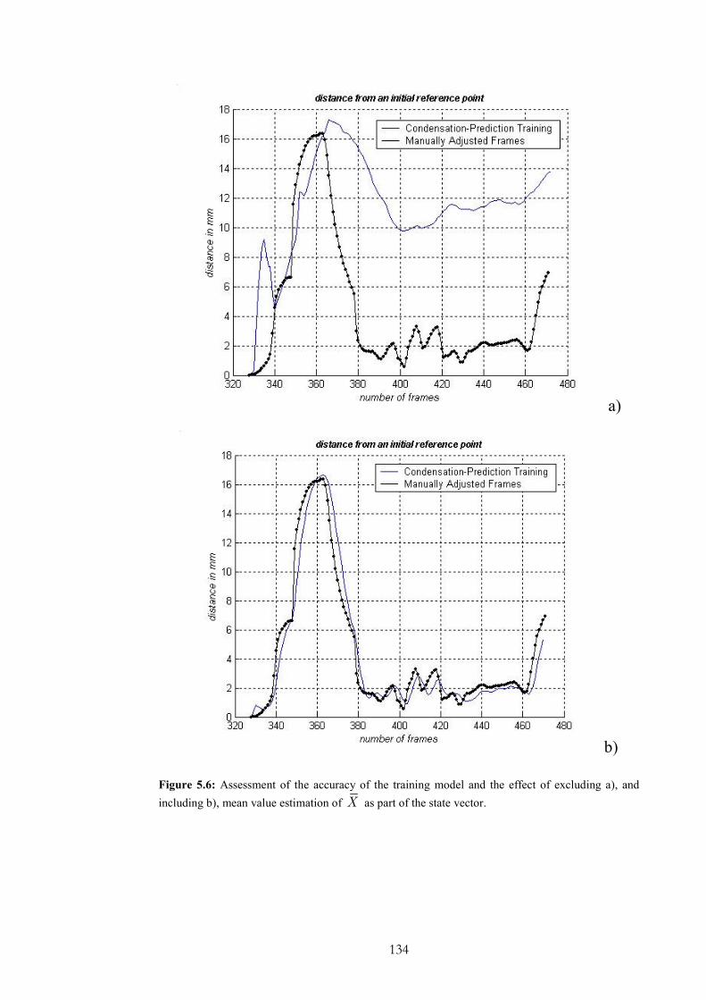
134
a)
b)
Figure 5.6: Assessment of the accuracy of the training model and the effect of excluding a), and
including b), mean value estimation of X as part of the state vector.

135
5.5 Experimental Design
In order to assess the accuracy of the proposed algorithm, an airway phantom made of
silicone rubber and painted with acrylics was constructed. The phantom has a cross
sectional diameter of 12cm at the opening and narrows down to 5cm at the far end. The
inside face was created such to give the surface a specular finish that looks similar to the
surface of the lumen. This phantom has been described in details in Chapter 4. A real-time,
six degrees-of-freedom Electro-Magnetic (EM) motion tracker (FASTRAK, Polhemus) was
used to validate the 3D camera position and orientation. The EM-tracker has an accuracy of
0.762mm RMS. The tomographic model of the phantom was scanned with a Siemens
Somaton Volume Zoom four-channel multi-detector CT scanner with a slice thickness of
3mm and in-plane resolution of 1mm. A CMOS camera and NTSC standard with frame
rate of 30fps was used.
For in vivo validation, bronchoscopy examination was performed in five patients according
to a standard clinical protocol. During the bronchoscope procedure two similar type
videoscopes (Olympus BF Type; with field of view 120°) were used. Video images from
the bronchoscope examination were transferred to digital videotapes in PAL format at
25fps. Since the original endoscopic video frames contain both the endoscopic image and
redundant black background, only the endoscopic view was digitized and cropped to
images of 454×487 pixels. All images were converted to grayscale before the pq-space
analysis. Similar to the phantom study, the CT images were acquired from the Siemens
Somaton Volume Zoom four-channel multi-detector CT scanner with a slice width of 3mm
and collimation of 1mm, and the acquisition volume covered from the aortic arch to the
dome of hemi-diaphragm. Pre-processing of the video images was necessary in order to
alleviate the effects of interlacing, lens distortion and unnecessary texture information. To
remove noise and image artifacts, anisotropic filtering was applied to each image.
5.5.1 Obtaining the Training Sequences
Training sequences were produced by the manual alignment of selected key frames.
Subsequently, both the position and orientation of intermediate frames can be estimated by
interpolating the measurements. For positional interpolation, cubic spline-based, piecewise
cubic Hermite and linear interpolation have been tested. Spline-based interplation can cause
some artefacts that do not reflect the actual dynamic motion behaviour of the camera. This
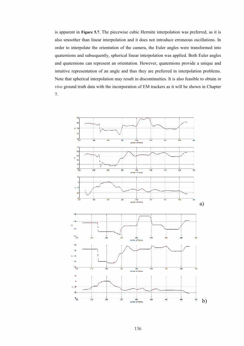
136
is apparent in Figure 5.7. The piecewise cubic Hermite interpolation was preferred, as it is
also smoother than linear interpolation and it does not introduce erroneous oscillations. In
order to interpolate the orientation of the camera, the Euler angles were transformed into
quaternions and subsequently, spherical linear interpolation was applied. Both Euler angles
and quaternions can represent an orientation. However, quaternions provide a unique and
intuitive representation of an angle and thus they are preferred in interpolation problems.
Note that spherical interpolation may result in discontinuities. It is also feasible to obtain in
vivo ground truth data with the incorporation of EM trackers as it will be shown in Chapter
7.
a)
b)
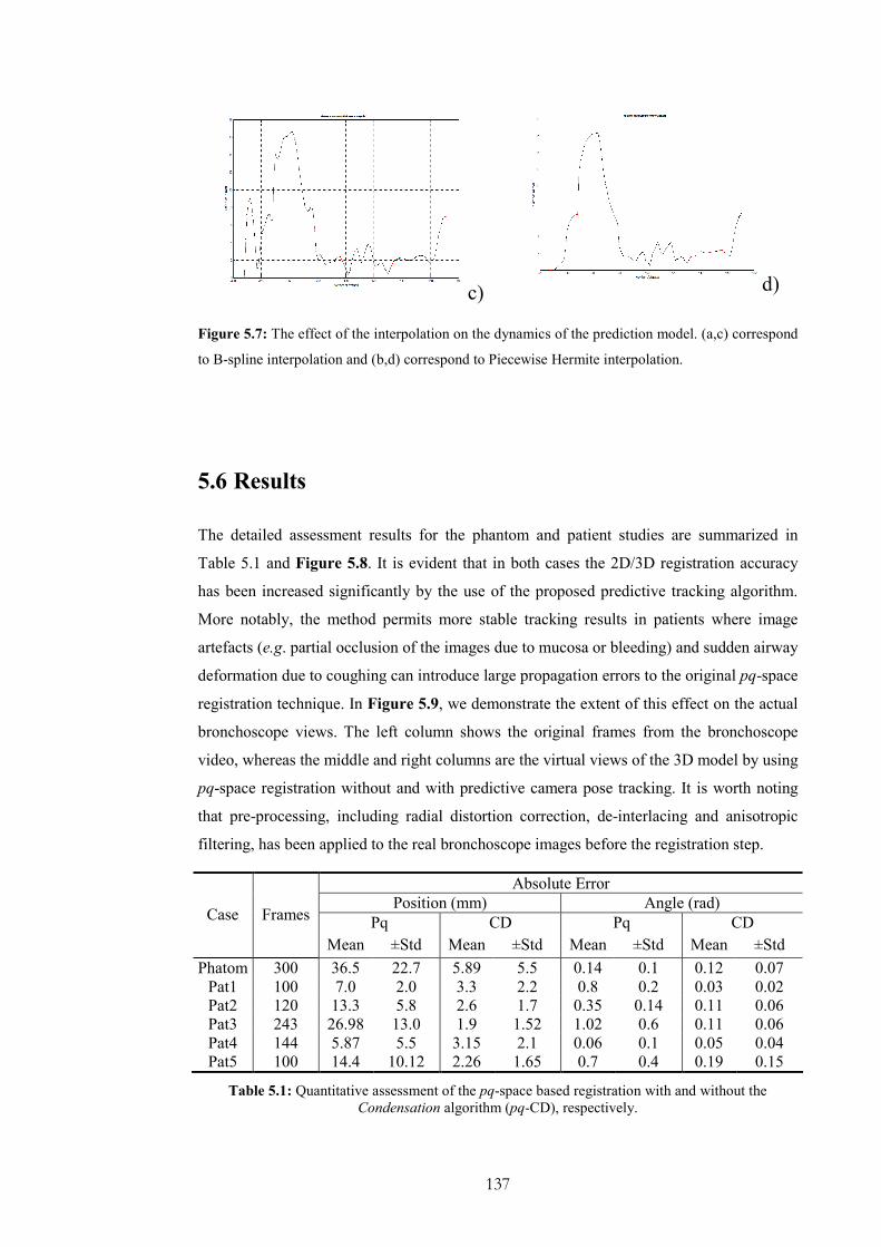
137
c) d)
Figure 5.7: The effect of the interpolation on the dynamics of the prediction model. (a,c) correspond
to B-spline interpolation and (b,d) correspond to Piecewise Hermite interpolation.
5.6 Results
The detailed assessment results for the phantom and patient studies are summarized in
Table 5.1 and Figure 5.8. It is evident that in both cases the 2D/3D registration accuracy
has been increased significantly by the use of the proposed predictive tracking algorithm.
More notably, the method permits more stable tracking results in patients where image
artefacts (e.g. partial occlusion of the images due to mucosa or bleeding) and sudden airway
deformation due to coughing can introduce large propagation errors to the original pq-space
registration technique. In Figure 5.9, we demonstrate the extent of this effect on the actual
bronchoscope views. The left column shows the original frames from the bronchoscope
video, whereas the middle and right columns are the virtual views of the 3D model by using
pq-space registration without and with predictive camera pose tracking. It is worth noting
that pre-processing, including radial distortion correction, de-interlacing and anisotropic
filtering, has been applied to the real bronchoscope images before the registration step.
Absolute Error
Position (mm) Angle (rad)
Pq CD Pq CD Case Frames
Mean ±Std Mean ±Std Mean ±Std Mean ±Std
Phatom 300 36.5 22.7 5.89 5.5 0.14 0.1 0.12 0.07
Pat1 100 7.0 2.0 3.3 2.2 0.8 0.2 0.03 0.02
Pat2 120 13.3 5.8 2.6 1.7 0.35 0.14 0.11 0.06
Pat3 243 26.98 13.0 1.9 1.52 1.02 0.6 0.11 0.06
Pat4 144 5.87 5.5 3.15 2.1 0.06 0.1 0.05 0.04
Pat5 100 14.4 10.12 2.26 1.65 0.7 0.4 0.19 0.15
Table 5.1: Quantitative assessment of the pq-space based registration with and without the
Condensation algorithm (pq-CD), respectively.

138
Angular Error
0
0.2
0.4
0.6
0.8
1
1.2
1 2 3 4 5
Subjects ID
MSE in rad
IR
COND
Positional Error
0
5
10
15
1 2 3 4 5
Subjects ID
STD in mm
IR
COND
Angular Error
0
0.1
0.2
0.3
0.4
0.5
0.6
0.7
1 2 3 4 5
Subjects ID
StD
in rad
IR
COND
Figure 5.8: Bar chart showing the quantitative assessment of the pq-space based registration with
and without the condensation algorithm.
Positional Error
0
5
10
15
20
25
30
1 2 3 4 5
Subjects ID
MSE in mm
IR
COND
139
5.7 Discussions and Conclusions
In this chapter, we have described the use of predictive camera tracking for increasing the
general accuracy and robustness of 2D/3D registration involved in virtual bronchoscope
modelling. A stochastic filter is used to resolve the inherent global ambiguity in tracking by
exploiting the temporal coherence of the camera tip. Particle filters, particularly the
Condensation algorithm, permits the use of multi-modal probability distributions and it is
not restricted to linear systems and white noise. Instead, it uses statistical factor sampling to
approximate any form of probability distribution without any assumptions. The results from
both phantom and patient data demonstrate a significant improvement in tracking accuracy
especially in cases where there is slight airway deformation and image artefacts. The
method effectively avoids the registration algorithm being trapped in local minima and
increases the overall accuracy. It is also able to recover when the image-based registration
has failed, because it does not use the previous camera pose to initialise the following
registration step.
It has been shown that the use of a second order ARG model is particularly effective for
bronchoscope camera motion prediction that it is highly restricted inside the tracheo-
bronchial tree. Another important feature of this model is the use of two previous camera
poses to estimate the subsequent camera positions. This contributes to the robustness of the
proposed framework against failures of the image-based algorithm. This is because the
system has a memory encoded in the form of particles. Particles tend to concentrate around
the areas indicated by the measurements. Subsequently, erroneous measurements that are
completely outside of the underlying neighbourhood of possible positions are rejected as
outliers.
The estimation of the parameters of both the auto-regressive motion model and the noise
distribution plays an important role in the algorithm proposed. In this work, the parameters
are estimated through a systematic procedure based on the principles of the maximum
likelihood learning. The main advantage of this approach is that it extends modular
learning. Modular training facilitates the incorporation of multiple sequences from different
patients during training. In bronchoscopy, ground truth data are difficult to be obtained.
Therefore, it is desirable to create a prediction model that is not patient specific. Our results
indicate that modular training can be successfully implemented when the mean of the
system is also a part of the state space. In practice, the mean typically varies from system to

140
system and it cannot be estimated by simply averaging the individual mean values. If the
mean value is not calculated properly, it can cause the rest of the terms to be falsely
estimated. In this case, the numerical error can be large enough to change the overall
characteristics of the system.
It should be noted that the proposed method can be further extended to multi-class motion
description such that the dynamic behaviour of camera navigation in different parts of the
tracheo-bronchial tree can be incorporated [141]. In this way, several auto-regressive
models can be utilised and trained to allow for more accurate predictions. It is also
necessary in practice to take into consideration of the technical skills of the operators and
separate them into different groups. It is also worth noting that temporal tracking has also
its limitations. Although it improves 2D/3D registration under airways deformation and
occlusion, it may also fail when prolonged image artefacts are encountered. The actual
quality of modular training also reduces with the number of degrees-of-freedom. Therefore,
it is more efficient to propagate separately the positional information from the angular state
space. Nevertheless, there is a relationship between changes in the camera position and
changes in the orientation. Further investigation is required to clarify how this information
can be incorporated in an efficient way.

141
Figure 5.9: The effect of airway deformation and partial occlusion of the image due to mucosa and
blood on the accuracy of the 2D/3D registration technique without (mid-column) and with (right-
column) predictive camera tracking.
142
Chapter 6
EM Trackers in Bronchoscope
Navigation
n the last two chapters, we have developed a pq-space based framework for 2D/3D
image registration. We have also demonstrated how temporal tracking can be used to
improve the overall system accuracy and robustness when severe artefacts are encountered.
From the in vivo experiments, it has become clear that image-based techniques have certain
limitations. Although the proposed pq-space based similarity measure is immune to lighting
parameters, airway deformation has so far only been considered qualitatively in an ad hoc
manner. In Chapter 4, local deformation of the airways is detected from temporal variations
of the pq distribution and the registration algorithm assumes that this deformation is
relatively small. For patient-specific bronchoscope tracking and modelling, however,
respiration and patient motion can introduce significant distortions to the tracheo-bronchial
tree. For the proposed algorithm to be clinically useful, further enhancement in effective
motion handling is necessary.
To this end, EM tracking devices offer an attractive solution. The latest generation of
miniaturised catheter tip EM tracking devices allow the insertion of the EM sensor into the
biopsy channel of the endoscope. This offers the potential for significantly improving the
robustness and accuracy of current registration techniques in the presence of large tissue
deformation. In this way, the camera position can be tracked during the whole procedure
with sub-millimetre accuracy and real-time response. The major advantage of these systems
is their immunity to the quality of the video frames, as well as the imaging artefacts
involved.
I
143
However, there are several challenges need to be addressed before these systems can be
safely applied to clinical simulation. The choice of the tracking system is influenced by a
number of parameters that depend both on the nature of the application and the required
level of accuracy. Ferromagnetic distortion, tissue deformation and patient movements
reduce the accuracy of these systems in clinical environments. Particularly in
bronchoscopy, respiratory motion and global shifting of the position of the patient can
interfere with the measurements of the EM tracker and subsequently reduces its
effectiveness. In this chapter, we will address the technical issues related to the use of EM
tracking devices for bronchoscope tracking, and emphasise on the issue of how to decouple
global and respiratory motion of the EM tracking data such that its reading can be
effectively used to guide the 2D/3D registration algorithm.
6.1 Positional Trackers in Medical Applications
Tracking devices are well known in image-guided surgery because they provide real-time
measurement and have stable performance compared to image-based fusion techniques
[149, 150]. In many surgical applications, it is important to correlate in real-time the intra-
operative field with the imaging space. For example, in neurosurgery tumours identified in
CT or MR images may be visually difficult to distinguish from the surrounding normal
tissue during surgery. In neurosurgery, optical tracking devices were developed in the early
1990’s and they gradually replaced neuronavigator arms, which have been used since the
end of 1980’s as passive intraoperative position systems. The main advantage of optical
tracking is that they are easy to handle and have fewer restrictions to the surgeon’s
movements.
Optical tracking systems provide the most reliable and precise position sensors available in
medical applications [151]. Objects are tracked by rigidly attaching retro-reflective spheres
or active infrared LED’s. The spheres can be detected by the camera system and used to
determine the location and orientation of the object. Infrared light is used for maximal
accuracy and decreased sensitivity to ambient light. Optical tracking provides an attractive
solution for tracking rigid tools due to its linearity, stability and accuracy. Compared to
ultrasound and EM trackers it offers a great potential in terms of accuracy and speed of
acquisition. Subsequently, it has been popular in surgical operations related to brain, spine
and general orthopaedics, in which it has been established as part of the standard clinical
practice. However, the method is constrained to the line-of-sight applications and thus it is
inappropriate for tracking flexible instruments inserted into patients.

144
6.2 Miniaturised Electro-magnetic Trackers
Recently, Electro-magnetic Tracking (EM) has made significant advances both in terms of
its accuracy and miniaturisation. Examples of such systems that can be used for MIS
include Aurora® (NDI), MiniBird
® (Ascension) and Magellan
® (Biosense Webster). They
are equipped with cylindrically shaped sensor coils to the size of the tip of a biopsy tool so
that they can be embedded in catheters and thin needles. The advent of miniaturised
trackers has a variety of potential clinical applications in computer aided interventions. The
needle probe is suited to computer-assisted minimally invasive drug delivery, biopsy, cyst
drainage, and electrode placement. The position and orientation of the flexible instrument
tip, such as endoscopes and catheters can be tracked accurately within the body. EM
trackers use the attenuation of oriented Electro-magnetic signals to determine the absolute
position and orientation of a tracker relatively to a source. The induced voltage level
provides information about both the distance from the transmitter to the receiver and the
axis-alignment between them. Boundaries of equal accuracy are found along a hemisphere
or sphere around the transmitter.
Although EM trackers are susceptible to ferromagnetic interference they can achieve a high
application accuracy after careful in situ calibration [152]. The potential clinical
applications of EM systems have already extended well beyond optical and mechanical
positional systems. Electro-magnetic systems that provide simultaneous
electrophysiological and spatial information have been approved for patient care and are
used in clinical practice. Such systems have been used in cardiac interventions, endonasal
sinus surgery and bronchoscopy [152-154]. EM systems also facilitate the development and
expansion of new diagnostic techniques and imaging modalities, such as Laparoscopic
Ultrasonography and neurorsurgical applications [155, 156]. This paragraph presents a brief
overview of the clinical applications and studies and the related challenges in EM tracking.
Electro-magnetic tracking technology (InstaTrackR CAS system) has been employed for
endonasal sinus surgery [152]. Endonasal sinus surgery is challenging because of the
presence of a variety of endangered vascular and neural structures in a very confined space
of the anterior skull base. For this kind of operations, computer-aided surgery is an
important tool for increasing the accuracy of orientation and becomes mandatory for
specific patient cases. For these systems, two EM sensors provide positional information
relative to the CT images. One sensor is located to the standard suction chamber and the
145
other is located on a headset worn by the patient during the surgical procedure. Similarly,
the possibility of extending the use of EM trackers in neurology has been shown in a
number of feasibility studies [156]. In the work by Zaaroor et al., the accuracy of an EM
system (Magellan system, Biosense Webster) is measured for image-guided neurosurgical
applications. The Magellan system was developed to provide real-time tracking of the distal
tips of flexible catheters, steerable endoscopes, and other surgical instruments, using ultra-
low electro-magnetic fields and a novel miniature position sensor for image-correlated
intra-operative navigation and mapping applications.
This EM system has been also tested for anatomically targeted ablations of the fossa ovalis,
which is found in the right atrium of the heart, and the left atrium [157]. Transvenous
catheter ablation is a treatment for many arrhythmias that involves the surgical removal part
of body tissue. Anatomical knowledge has important role in treating arrhythmias, such as
atrial fibrillation and non-idiopathic ventricular tachycardia. Although fluoroscopy is the
main intra-operative imaging modality, it provides limited information to localise the
catheter position in relation to the cardiac structures and expose both the patient and
medical staff to high doses of ionising radiation. Furthermore, the arteries can only be made
visible by inhaling a contrast agent, which subjects the patient to additional risks. Dickfeld
et al. [157] suggests stereotactic catheter guidance for cardiac applications. The EM system
is superimposed on three-dimensional MR images using fiducial markers. This allowed the
dynamic display of the catheter position on the true anatomy of previously acquired MRI in
real-time.
In surgery, EM tracking technology has also been used to provide surgeons with important
spatial cues during Laparoscopic Ultrasonography (LUS), so they can orient oblique
images with few constrains on positioning the laparoscopic port [155]. The key component
of this visualisation technique is that it shows how the ultrasonography plane interacts with
the aorta and thoracic skeletal anatomy. LUS is the most sensitive method for detecting
hepatic metastasis and it is also a mean of identifying stones during laparoscopic
cholecystectomy. However, one of the major problems is in interpreting LUS images
because they are not obtained in conventional orientations, such as transverse or sagittal
planes. This limits the adaptation of LUS in clinical practice, since both novice and
advanced ultrasonographers experience difficulty.

146
6.2.1 Accuracy Assessment and Metal Calibration of EM Trackers
There are a number of evaluation criteria for EM trackers:
(1) Resolution - It is related to the ability of the tracker to measure different points in
space, and subsequently, the numerical accuracy of the system. The accuracy of a
system is usually affected by whether the sensor moves or not and thus, it is
described as static or dynamic, respectively.
(2) Registration - It refers to the correspondence between actual position and
orientation and reported position and orientation. Calibration processes are used to
measure and adjust for the differences between reported and actual position.
(3) Drift - It is a gradual increase in tracking error over time.
(4) Jitter - It is a fluctuation in the reported position/orientation of the sensor.
(5) Phase Lag - It is the time that takes the sensor to report its position and it is related
both with the data generation and the transmission process.
(6) Update Rate - It is the number of tracker position/orientation samples per second
that are transmitted to the receiving computer. Higher update rates do not
necessarily imply better accuracy. An upper bound is determined by the
communications rate between computer and tracker and the number of bits that
encode the pose information.
(7) Range - Positional range refers to the working volume of the system, since the
accuracy of EM tracking systems decreases with distance. Orientation range refers
to the set of sensor orientations that the tracking system reports with a given
resolution.
(6) Interference and noise. Inaccuracies might occur due to external object and Electro-
magnetic fields. Random variations in an otherwise constant reading may also
occur and they are related to the static accuracy of the system.
(8) Physical dimensions - This refers to the size, mass and any other special
characteristic that affects the feasibility and function of the tracking system under a
specific application.
147
(9) Multiple sensors - This is related with the ability of the system to track multiple
points within the same volume.
Although AC magnetic trackers are accurate and can provide high update rates, they are
particularly sensitive to eddy-currents and ferromagnetic environment. The Aurora EM
system has been evaluated by a number of research groups [158-163] and has been used in
numerous clinical as well as phantom studies of image-guided applications [154, 164-166].
It represents a new generation of DC magnetic trackers with increased accuracy and
stability even in ferromagnetic environments [164]. The basic system consists of a control
unit, sensor interface devices and field generator and it enables the coils to be tracked in
five degrees-of-freedom (three spatial and two rotational coordinates). The sensors can be
as small as 0.9mm in diameter and 8mm in length. According to manufacturer’s
specifications, the sensors have a positional accuracy of 1-2mm and angular accuracy of
0.5-1 degree. The system’s dynamic rate is its maximum data rate, which is equivalent to
45Hz. The measurement volume is 50 by 50 cm, located 50mm from the field generator.
Typically, in the operating room there are various materials, such as closed metallic loops,
wire guides, catheters and monitors that interfere and distort the EM sensor measurements.
In addition, their accuracy depends on the distance between the transmitter and the sensor.
As opposed to optical tracking, the useful field-of-view is rather small. One possible
approach to overcome this problem is to design a hybrid tracking system, using an
additional optical tracking tool to monitor displacements of the emitter [158]. Nevertheless,
the susceptibility of EM tracking systems to EM interference is by far the greater obstacle
in the acceptance of these systems in standard clinical practice. Subsequently, there are
numerous studies testing the nature of the EM distortion caused by the presence of different
ferromagnetic materials in the operating room, as well as the development of techniques
that improve the measurement accuracy.
Hummel et al. [158] has tested the Aurora system to examine its accuracy under the
influence of: (1) closed wire loops with different radii, (2) guiding wires (endoscopes) with
different configurations of loops, (3) ultrasound scan probes near to the emitter and sensor,
(4) a mobile C-arm fluoroscopy unit, (5) an optical tracking tool, (6) an endoscope with a
radial ultrasound scan head, and (7) a needle holder, biopsy forceps and a drill handle.
Wilson et al. [163] also tested Aurora within a CyberKnife radiosurgery suite. CyberKnife
is a non-invasive, frameless, stereotactic radiosurgery device used to ablate tumours within
the brain, spine, chest and abdomen. One of the aims of the work was to determine the
accuracy and device behaviour with the presence of ionising radiation. Although, there are
noticeable trends in the Aurora system performance with and without the presence of
148
ionising radiation, the overall effect of measurement accuracy is minimal. On the other
hand, the tracker is more sensitive to distortions caused close to the emitter rather than to
the sensor. The deviations also depend on the relative orientation between emitter and
sensor, with the worst orientation having the sensor directed towards the field generator and
the best orientation being orthogonal. In the case of a biopsy tool close to the sensor the
distortion is negligible.
Collecting precise information on the nonlinear local error and calibrating the EM tracking
system can compensate the influence of the metallic equipment. An effective way to collect
reliable positional information is by using an optical tracking system, such as Polaris,
which determines the orientation and position of tracked objects relative to a camera system
[160, 167]. Robotic arms can be also used but they carry the risk that their metal bases
interfere with the EM tracking measurements. Once the data have been collected, several
tracking calibration methods can apply to find a mapping function between the gold
standard data provided from optical tracking and the EM data distorted from EM
interference. Kindratenko [168] presents a good survey on Electro-magnetic position
tracker calibration techniques, which are mainly used in virtual reality applications, such as
the CAVE (Cave Automatic Virtual Environment). Most methods, however, assume that
position displacements depend only on position and do not change with orientation.
Wu et al. [167] indicates that this assumption may be true for smooth distortions, but it
does not hold for the Aurora in a clinical setup. Chung et al. [160] also suggests that it may
not be adequate to obtain static measurements when performing the calibration, since the
accuracy of EM trackers is reduced when tracking objects are in constant motion.
Subsequently, Chung et al. [160] proposes a freehand calibration technique that
incorporates these requirements. It allows for free movements of the calibration object and
provides a mechanism of interdependence between positional and angular correction. To
ensure smooth interpolation of 2C continuity over the six degrees-of-freedom that
describes the position of the EM sensor, a radial basis spline framework is extended to cater
for the non-Euclidean nature of orientation space. While current calibration techniques
offer a factor of improvement of around 1.5, the second generation of extra-immune EM
systems has also become available recently [161]. These systems report accuracy of sub-
millimiter in the presence of ferromagnetic objects common in the operative room and open
the way of wider use of EM systems in computer aided surgery.

149
6.2.2 EM Tracking under Tissue Deformation and Patient Movements
Crucial to the success of EM endoscope tracking is the alignment between the EM data and
the pre-operative images. When the anatomical structure depicted on the pre-operative
images does not deform during operation then a rigid transformation between the EM
tracking coordinate system and 3D data can easily established based on landmark
correspondences. Subsequently, a least-square approach is used similar to [169, 170],
which offers an optimum in least-square sense closed-form solution and it requires a
minimum number of three non-collinear point correspondences. This methodology is
common in orthopedics and neurosurgery and generaly in optical tracking, because the
related anatomical structures are relatively rigid and apparent landmarks in both pre-
operative data and intra-operatively are easily identifiable. Furthermore, the position of the
patient can be easily tracked, by introducing additional sensors, for example attached to the
head and so on.
However, relating the EM tracking data to a static pre-operative scan can be particularly
challenging when flexible instruments and catheters are tracked inside the body. This is due
to tissue deformation and global shift of the position of the patient during operation. Tissue
deformation can result from tissue-tools interaction, cardiac contraction, respiratory motion,
organ function and internal shift of the organ as the patient changes position. This problem
has been reported to numerous research studies [154, 157, 171] and various motion
compensation techniques have been developed [166]. For example, Dickfeld et al.
investigated whether stereotactic catheter guidance based on EM tracking can place
radiofrequency (RF) ablations at well-defined anatomical targets, within the lateral wall of
left atrial appendage, identified on MRI. In the work by Dickfeld et al. [157] is recognised
the effects of respiratory motion to the accuracy of the technique and attached a reference
catheter on the chest of the animals to improve the accuracy of image registration during
respiratory or animal position changes. Respiratory motion compensation is well known in
radiotherapy, where a certain dose of radiation needs to be delivered in the cancerous target
with minimal effect on the surrounding healthy tissue.
In the work by Timinger et al. [166] also used an EM system (Aurora) to locate the catheter
during navigation within the coronary tree. The image-guided system was extended to
compensate for cardiac contraction and respiratory motion. Cardiac contraction is
compensated by gating the catheter position. In this process only those images acquired
during the rest phase of the heart are used for the image-guided system. An affine model is
used to compensate for the respiratory motion. This model is driven by a parameter, which
indicates the current state of the motion. Such a parameter can be the location of the edge of

150
the diaphragm, which moves along with respiration. However, a correlation between this
parameter and the resulting effect on the organ has to be identified. Assuming that this
correlation can be described by an affine model, point correspondences of the cardiac
phantom between fully exhaled phase and fully inhaled phase was extracted and
subsequently a least square minimisation approach was employed to recover the parameters
of the affine model. The work by Timinger et al. [166] based their methodology on the fact
that the movements of the heart and those of the diaphragm are similar due to the
anatomical neighbourhood. Subsequently, they simulated respiratory motion induced to the
artificial coronaries by a rotation.
There is high correlation between the motion of the needle placed in the liver and the
motion reported from a sensor attached on the sternum of the patient [172]. Subsequently,
an affine model was used to compensate for the error. However, it was also indicated that
there is the need to create more sophisticated models that account for tissue warping. In
general, motion of internal human organs may be complex with high non-rigid components.
This implies that simple mathematical models may fail to predict the deformation of more
complex anatomical structures, such as the tracheo-bronchial tree. For this reason it may
neither be adequate nor straightforward to associate the motion of an externally tracked
point to the internal motion of an organ. Nevertheless, the importance of motion
compensation in successful integration and clinical application of EM medical devices has
been widely recognised.
6.3 EM Tracking in Image-Guided Bronchoscopy
Miniaturised EM trackers have been also used in image-guided bronchoscopy to accurately
display the position of the tip of the flexible endoscope in pre-operative CT images [74,
154]. Bronchoscopists mainly rely on the endoscopic view to navigate in the airways and
acquire tissue samples. However, this results in poor diagnosis when transbronchial needle
aspiration is performed to detect extraluminal lesions. Moreover, during transbronchial
forceps biopsy the bronchoscopist relies on a C-arm fluoroscopy for guidance. Two-
dimensional fluoroscopy cannot accurately provide the 3D position of the lesion, which
frequently results in missing the target. EM tracking has the potential to facilitate
bronchoscopy procedures by tracking the tip of the flexible instruments.
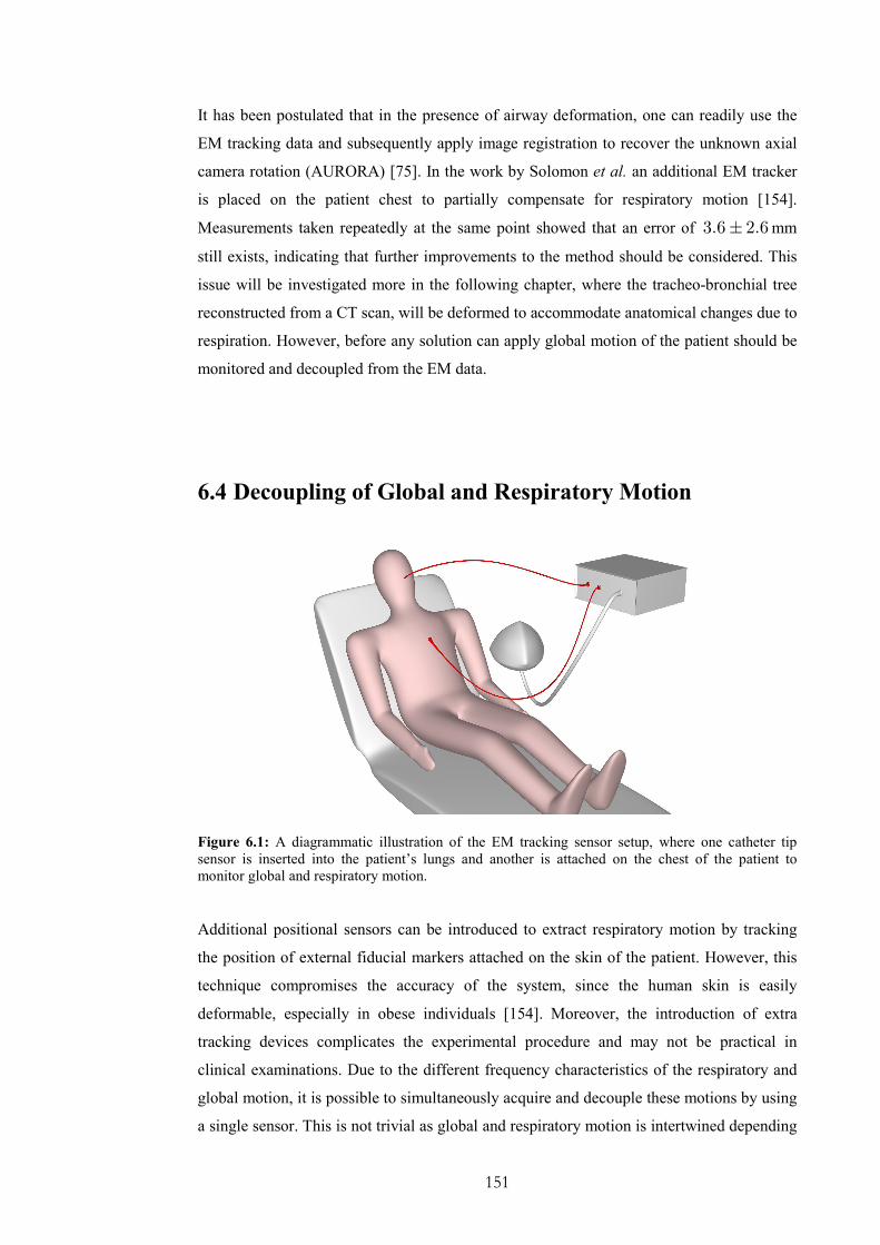
151
It has been postulated that in the presence of airway deformation, one can readily use the
EM tracking data and subsequently apply image registration to recover the unknown axial
camera rotation (AURORA) [75]. In the work by Solomon et al. an additional EM tracker
is placed on the patient chest to partially compensate for respiratory motion [154].
Measurements taken repeatedly at the same point showed that an error of 3.6 2.6± mm
still exists, indicating that further improvements to the method should be considered. This
issue will be investigated more in the following chapter, where the tracheo-bronchial tree
reconstructed from a CT scan, will be deformed to accommodate anatomical changes due to
respiration. However, before any solution can apply global motion of the patient should be
monitored and decoupled from the EM data.
6.4 Decoupling of Global and Respiratory Motion
Figure 6.1: A diagrammatic illustration of the EM tracking sensor setup, where one catheter tip
sensor is inserted into the patient’s lungs and another is attached on the chest of the patient to
monitor global and respiratory motion.
Additional positional sensors can be introduced to extract respiratory motion by tracking
the position of external fiducial markers attached on the skin of the patient. However, this
technique compromises the accuracy of the system, since the human skin is easily
deformable, especially in obese individuals [154]. Moreover, the introduction of extra
tracking devices complicates the experimental procedure and may not be practical in
clinical examinations. Due to the different frequency characteristics of the respiratory and
global motion, it is possible to simultaneously acquire and decouple these motions by using
a single sensor. This is not trivial as global and respiratory motion is intertwined depending

152
on the projection axes. In the subsequent sections, we will present a new technique that
uses wavelet analysis to identify and filter out episodes related to coughing and extreme
breathing patterns, and a principal component analysis based method to retrieve the hidden
respiratory pattern of the EM position sensor.
6.4.1 Principal Component Analysis
Given that the dominant variation of the signal is due to respiratory motion and it has a
constant direction during a given time window, then principal component analysis can be
employed to decouple it. The principal vector is expected to lie on the same plane over time
and, thus projecting the signal on this plane can isolate the signal variations due to
respiration. We define as f the positional vector over time of the MagTrax (Traxtal
Technology) reference sensor attached to the chest. Typically, the respiratory pattern has a
higher frequency than positional drift of the patient, a box kernel ( )tδ is convolved to each
axis of the motion sensor such that
( ) ( ) ( ) ( )*f t f t f t tδ= − ∗ (6.1)
The width of the kernel ( )tδ is chosen to be approximately half respiration cycle (3sec) so
that the DC component is filtered out. Here the DC component includes the static position
of the patient, as well as the positional drift and the motion of the bronchoscope with lower
frequency than respiration.
In discrete form, the samples over time can be represented as:
( ) ( ) ( )* * *f , f , .... ft w t t w t t t w t− ⋅∆ − ⋅∆ +∆ + ⋅∆ (6.2)
where t∆ expresses the sampling time interval and w is an integer that corresponds to
each sample in a kernel that has a typical length of 30 sec.
Subsequently, a matrix h is defined for each time sample as:
( ) ( ) ( ) ( )* * *f , f , .... fT
h t t w t t w t t t w t = − ⋅∆ − ⋅∆ +∆ + ⋅∆ (6.3)

153
h has dimension of ( )2 1 3w + ⋅ , because it includes positional information of the
bronchoscope in a 3D coordinate system ( ), ,x y z . Note that ( )h t is the mean of ( )h t .
Therefore, the covariance matrix is produced as:
( ) ( ) ( )( ) ( ) ( )( )TM t h t h t h t h t= − ⋅ − (6.4)
The principal vector ( )p t is estimated from the eigen-decomposition of the covariance
matrix. Finally, r is a scalar vector, which represents the decoupled respiratory motion.
Each element of r , ( )r t , is estimated as the projection of ( )*f t on the principal vector
( )p t .
( ) ( ) ( )*fr t t p t= ⋅ (6.5)
6.4.2 Wavelet Analysis
During bronchoscope examination, coughing involves major distortion of the airway thus
those video sequences should be isolated during image based modelling. In order to
identify these episodes wavelet analysis was used [173]. Wavelet analysis provides a
localised frequency analysis and has the potential to analyse signals that contain multiple
non-stationary or transitory signal characteristics, such as drift and abrupt changes. On the
other hand, Fourier transform assumes that a signal is stationary, which implies that it has
constant statistical parameters over time. The issue of stationarity depends on the size of the
sampling window. During bronchoscope examinations, the signal cannot be approximated
as stationary and thus the wavelet analysis is inherently more suitable. The main
advantages of the method are both its ability to perform local analysis and to preserve time
information. In the other words, wavelets represent a windowing technique with variable-
sized regions that allow the use of long time intervals when low frequency information is
available, and shorter intervals when high frequency information is present.
Let ( )tψ be a function in the Hilbert space ( )2L R of measurable, square-integrable one-
dimensional functions with an average of zero. The wavelet transform of a function ( )f t at
scale j and position t is given by the convolution product:
( ) ( )j jW f t f tψ= ∗ (6.6)

154
Figure 6.2: Wavelet analysis: X, Y and Z positional data has been acquired from an EM tracker
attached on the skin of a healthy subject in order to assess the wavelet technique of filtering sudden
movements similar to those that are introduced in a bronchoscopy session when the patient coughs.
We used Daubechies (db10) mother wavelets to analyze the signals.
In multiscale edge analysis, ( )tψ is usually chosen to be the derivative of some smoothing
function, and thus the local maxima of ( )Wf t indicate the positions where sharp signal
155
variations occur. In order to identify these variations, we define an energy function e with
threshold ξ .
( ) ( )10
j
j
e t W f t ξ<
= >∑ (6.7)
6.5 Experimental Design
Two experiments have been conducted in order to validate our technique. Firstly, the EM
tracker was attached on the subject chest to monitor normal breathing and coughing. The
subject was asked to cough at a particular time, while slight global motion was introduced.
An example is demonstrated in Figure 6.2 and has been used to validate the wavelet
technique. Secondly, positional data has been acquired from two Aurora EM trackers. The
first sensor was placed on the chest of the immobile volunteers to be used for respiratory
gating. The second one was placed on the chair, in order to monitor the global motion used
for validation. In this case, the positional difference of the two sensors should be purely due
to respiration. Subsequently, we applied the decomposition method mentioned above to
extract respiration from just one sensor attached to the chest. The aim is to see the extent to
which the respiratory motion can be recovered from this sensor alone. Eight subjects have
been recruited for this study. During the experiment, they were asked to keep their body
completely immobile, while they were breathing normally. Their respiration has been
monitored for about 2 minutes. Global motion was introduced either by moving the EM
field emitter or the base of the chair smoothly.
6.6 Results
Figure 6.2 and Figure 6.3 demonstrate the wavelet analysis of the X, Y and Z positional
data that have been acquired from an EM tracker attached on the skin of a healthy subject.
The wavelet coefficients are plotted for each signal component. Figure 6.3 represents the
energy function of the X-wavelet coefficient graph that has been defined within equation
(6.7). The time interval where the patient coughs shows up clearly as a pick at around 1000
time samples that corresponds to 88 sec.

156
Figure 6.3: The enrgy function after analyzing the X-motion signal. Similar results have been
acquired from analyzing either the Y or the Z component.
In Figure 6.4, the respiratory motion decoupling technique is demonstrated. Figure 6.4 (b)
illustrates the x, y, z positional component of the data received from the EM tracker
attached on the chest of one of the subjects, while Figure 6.4 (a) illustrates the x, y, z
positional component of the data received from the EM tracker attached on the chair.
Global motion has been introduced by moving slightly the field emitter (Aurora). Figure
6.4 (c) represents the recovered respiratory component after applying the proposed
technique of Section 6.4 to the data received from the EM tracker on the subject’s chest. In
order to validate our technique the correlation between the recovered waveform (Section
6.4) and the waveform estimated by applying principal component analysis to the vector
between the two EM tracker tool tips has been calculated for eight subjects. Table 6.1
demonstrated the results, which indicate a high degree of correlation.
Subjects 1 2 3 4 5 6 7 8
Correlation 0.918 0.962 0.805 0.794 0.879 0.791 0.786 0.687
Table 6.1: Correlation of the waveform estimated by the suggested respiratory decoupling motion
technique with the waveform estimated by relative position of two sensors.

157
a)
b)
c) Figure 6.4: Example position traces sampled by the EM tracker and the extracted respiratory motion
pattern.
6.7 Discussions and Conclusions
Thus far, tracking devices have been integrated into a number of image-guided surgery
applications. The most successful examples are in neurosurgery and orthopaedic surgery.
Accuracy and stability of these systems is critical to patient health and the outcome of the

158
operation. Currently, the most reliable and precise position sensors available in surgical
applications are optical tracking systems. The main advantage of these methods is that they
are not affected from ferromagnetic distortions, while they have a large operative volume.
Unfortunately, optical trackers are limited to the line-of-sight applications and thus they are
inappropriate for tracking flexible instruments inserted in patients.
Recently, the technological advances of miniaturised EM tracking sensors have allowed
their insertion in the biopsy channel of flexible endoscope and permit real-time tracking of
the endoscope tip inside the body cavity. Although the inherent mechanism of EM tracking
devices is inferior to the corresponding mechanism of optical trackers, it does not imply
that their application accuracy is always inferior. In fact, optical trackers can only be used
to track fiducial markers that are always rigidly attached on the skin or on the rigid surgical
tools. Nevertheless, this is compromised by the deformable nature of soft tissue and the
non-perfect rigidity of the tools. Furthermore, continuous tracking is also compromised
from the line of sight constraint.
It is important to realise that mechanical accuracy of a positional system is different from
application accuracy. For example, an EM system with manufacturing specifications of
sub-millimetre accuracy, under the influence of metal and tissue deformation, it may
provide measurements that are several centimetres away from the correct positions. This
indicates that the limiting factors in the use of these systems in practice are not their
inherent inaccuracy but the lack of appropriate methods to exploit their capabilities. Most
of the current image guided systems rely on a preoperative-static scan without any update
to allow for tissue deformation with relation to patient movements during the procedure.
Therefore, methods should be developed to compensate for tissue deformation and to
monitor the global position of the underlying anatomy with relation to a fixed coordinate
system. This, however, is not a trivial task, particularly in bronchoscopy. The internal
motion of the airways is difficult to be modelled adequately and it is not straightforward
how it correlates with the motion of externally tracked points. There are two goals to be
achieved. The first aims to decouple global from respiratory motion and the second is to
model the tracheo-bronchial tree motion during respiration.
In the work presented in this chapter, we have developed a novel method of decoupling
respiratory motion from the signal received from an EM tracker attached to the chest. We
used wavelet analysis to filter out episodes due to coughing and other extreme breathing
patterns. Principal component analysis has been employed to decompose the respiratory
cycle from global motion. It should be noted that the basic assumption used for respiratory
159
motion decoupling is that the global positional drift has a relatively low frequency in
comparison to respiratory cycles. When there is sudden motion involving large
acceleration, it is likely that rapid changes in sensor readings will be introduced. In this
case, the algorithm based on principal component analysis will lead to detection errors.
Since we have used wavelet analysis to sense rapid sensor movement, these events will also
be isolated along with coughing and extreme respiratory motion. The results in this study
indicate that episodes related to coughing can easily identified and filtered out and the
respiratory motion component can be reliably extracted. The suggested technique can
facilitate a 2D/3D registration regime under deformation and increase the accuracy of the
registration process. Further clinical approval needs to be done to investigate its efficiency.
In the next chapter, we will demonstrate that it is also possible to capture the airways shape
variability during respiration and use this prior knowledge to facilitate the non-rigid 2D/3D
registration framework. In this way, the EM devices can be utilised directly in the
registration process to further enhance the registration accuracy of the proposed pq-space
2D/3D registration method.
160
Chapter 7
Non-Rigid 2D/3D Registration with
Statistical Shape Modelling and EM
Tracking
n the previous chapter, we have demonstrated the potential value of EM tracking for
2D/3D registration. We have shown that continuous tracking of the bronchoscope is
difficult with image-based registration algorithms alone and the method can fail if extreme
breathing patterns are encountered. Image artefacts caused by mucosa, bubbles and
bleeding during a typical bronchoscopy examination can also pose significant challenges.
The introduction of in vivo catheter tip EM tracking means that it is now possible to
explicitly incorporate airway deformation into the registration framework.
The incorporation of airway deformation to the existing 2D/3D registration framework,
however, is a difficult task. This is due to the potentially very large degrees of freedom
involved in simultaneous tracking of the camera pose and structural changes. At first
glance, it may seem that the use of a 5 DoF catheter tip EM tracker reduces the original
2D/3D registration to only a 1D problem. It has been postulated that in the absence of
airway deformation, one can readily use the EM tracking data to recover the unknown axial
camera rotation [75]. For situations where large non-linear deformation is encountered in
vivo experiments, however, the nature of the problem is much more difficult than what it
first appears. This is because the EM tracker reports only the position and orientation of the
bronchoscope camera in relation to the fixed, world coordinates. When this information is
used to guide the registration of the airway structure reconstructed from the tomographic
data, a large displacement due to airway deformation can be observed. When this EM
tracking information is used to initialize the 2D/3D registration, it has been found that the
I
161
initial view can often be completely outside of the bronchial tree. This initialization is in
fact inferior to the traditional image based approach, as in this case the camera view is
always in synchrony with the moving frame of reference of the deforming airways. For this
reason, direct mapping of the EM tracking measurements to the static preoperative CT
images is not appropriate, and its practical use must be considered with the deformation of
the airways.
In this chapter, we will present a non-rigid 2D/3D registration framework and its phantom
validation for subject-specific bronchoscope simulation. The method makes use of a 5 DoF
miniaturised catheter tip EM tracker such that the position and orientation of the
bronchoscope can be accurately determined. This allows the effective recovery of unknown
camera rotation and airway deformation, which is modelled by an Active Shape Model
(ASM). It is demonstrated that ASM can capture the intrinsic variability of the tracheo-
bronchial tree during breathing. ASM is specific to the class of motion it represents and this
enables the reduction of the number of parameters that control the deformation.
Subsequently, the optimisation procedure is greatly simplified and pq-based registration as
described in Chapter 4 is performed to recover both the camera pose and parameters of the
ASM. Detailed assessment of the algorithm is performed on a deformable airway phantom,
with the ground truth data being provided by an additional 6DoF EM tracker to monitor the
level of simulated respiratory motion.
7.1 Deformable 2D/3D Registration
Figure 7.1 provides a schematic illustration of the proposed registration framework. Given
a number of volumetric images at different respiratory phases of the tracheo-bronchial tree,
an ASM capturing the intrinsic deformation of the airway is created. Based on the control
points of the ASM, Radial Basis Functions (RBFs) are used to warp the 3D mesh to reflect
the structural deformation induced. 2D/3D registration is then used to recover both the
parameters of the ASM and the pose of the bronchoscope camera. We demonstrate that by
modelling the deformation of the airways with ASM, it is possible to capture intrinsic
variabilities of the tracheo-bronchial tree based on images acquired at different phases of
the respiratory cycle. In this way, the dimensionality of the non-rigid 2D/3D registration
problem can be significantly reduced, thus leading to a more robust registration framework
that can be deployed to patient bronchoscope examinations.

162
EM 5DoF
Sensor Data
Intra-Operative
3D ModelsRespiratory
Motion
Cardiac
Motion 2D/3D Registration
Optimal
Deformable
Model
Optimal
Pose
Non-Rigid 2D/3D Registration
Airway
Deformation
Endoscope
Video
ASM & RBF
Initial
5DoF pose
Figure 7.1: A schematic illustration of the proposed non-rigid 2D/3D registration framework with 5
DoF EM tracking and ASM for deformation modelling.
7.1.1 Deformation Modelling of the Airway Tree
In order to design an efficient non-rigid 2D/3D registration, prior knowledge about the
airways deformation during respiratory motion is required. Deformable models can
accommodate the variability of biological structures over time and across different
individuals. As it has already been mentioned in Chapter 3, deformable models have been
proved to be effective in tracking anatomical structures and they are used extensively in
non-rigid registration for formulating transformation models. Deformable models are
constructed under the influence of geometry, physics and approximation theory [91].
Geometry serves to represent object shape, physics imposes constraints on how the shape
may vary over space and time, and optimal approximation theory provides the mechanisms
for fitting the models to the measured data.
As an example, prior knowledge about the deformation of the lungs can be derived by
monitoring the tracheo-bronchial tree during respiration in order to determine how the
shape changes over time. This can be accomplished by scanning lungs in different
respiratory phases [95]. Alternatively, anatomical and physiological models of respiration
can be incorporated [174, 175]. In the work by Kaye et al. [50], a simulation system that
combines anatomy and respiratory mechanics has been developed based on a physical
model. The lungs are considered as a single-compartment, viscoelastic structure, and the
classic mechanical model based on observable variables such as pleural pressure change,
lung volume change, and airway pressure is used. However, the contraction of the intra-
thoracic tree depends on the surrounding structure and the biomechanical properties of the

163
elastic tissue. In practice, biomechanical modelling of the airways is not trivial because it
requires in vivo measurements of the tissue properties of the vessel lumen.
In the work by Garrity et al. [95], a dynamic model for the lung lobes and the airway tree
has been developed. A model of the first four to five generations of the airway tree has been
created by segmenting the visible human CT data. The algorithm assumes that each branch
is a rigid cylindrical tube with a constant diameter and a dichotomous subdivision system.
Parameters for the daughter branches are determined by equations defining the
relationships between the air flow and the diameter, angle, and length of the branches. Once
the lung lobes and airway tree are finalized, the respiratory motion is modelled based on
high-resolution 4-D respiratory-gated CT data obtained from a normal human subject. The
data consists of two CT scans taken at two different time points of the respiration cycle.
One scan was taken at 5% of total lung capacity (TLC) and the other scan was taken at 40%
of TLC. The limitations of this approach are that the parameterisation is based on splines
and requires a large amount of parameters. Furthermore, the airways are over-smoothed and
the method does not offer a patient specific deformation model of the lungs.
7.1.2 Active Shape Models
In this thesis, we suggest using the Point Distribution Model (PDM) of the ASM for the
modelling of airway deformation to ensure that a compact representation of the deformation
of all the control points can be captured by the principal modes of shape variation. In this
way, the degree-of-freedom during deformable 2D/3D registration is only dictated by the
number of modes chosen plus the extra degree-of-freedom introduced by the unknown axial
rotation of the endoscope.
ASMs are parametric deformable models that deform in ways that are consistent with the
class of shape and motion they represent [40]. This is defined by the boundary point
distribution of a number of shapes, called a training set. To ensure that the ASM captures
the intrinsic shape rather than the corresponding landmark point variations, all shapes in the
training set should be aligned so as to minimise the distance variance of corresponding
control points. Subsequently, Principal Component Analysis (PCA) is applied to the PDM
to extract the statistical modes of variations that describe these shapes.
The intuitive benefit of ASM derives from the fact that for most deformable models the
landmark points are not moving independently, so the intrinsic dimension is significantly

164
lower than the number of control points. Let is be a vector describing the n control points
of the ith shape of the deformable model.
( )0 0 0 1 1 1, , , , , , , , , ,T
i i i i ik ik ik in in ins x y z x y z x y z− − −= … … (7.1)
Each sample in the training set can therefore be represented by a single point in a 3n-
dimensional space. A set of N deformable shapes (6 for this study) results in N points in
the 3n-dimensional space. These points in general lie within a region of the shape space,
which is called the ‘allowable shape domain’. Given that every 3n-dimensional point within
this domain gives a set of landmarks whose shape is similar to those in the original training
set, the variability of the shape can be modelled in a systematic way in the remapped space.
By assuming that the allowable shape domain is approximately ellipsoidal, its centre can be
calculated as the mean shape s , i.e.,
0
1 N
i
i
s sN =
= ∑ (7.2)
Subsequently, the principal axes of the ellipsoid fitted to the data are calculated by applying
PCA to the data. Each axis gives a mode of variation, which represents the way that the
landmark points tend to move together as the shape varies. For each shape in the training
set, the deviation from the mean ids is calculated to form the covariance matrix S :
0
1 NT
i i
i
S ds dsN =
= ∑ with i ids s s= − (7.3)
In this way, any point in the allowable shape domain can be modelled by taking the mean
shape and adding a linear combination of the eigenvectors of the covariance matrix, i.e.,
s s Pb= + (7.4)
where ( )1, , tP p p= … is the matrix of the first t eigenvectors. Therefore, new shapes are
generated by varying the parameters kb within the suitable limits for them to fit to the
training set. The limits for kb are derived by examining the distributions of the parameter
values required to generate the training set. In this study, the set of the parameters
1, , tb b… is chosen by assuming that the plausible shape variations lie within three
standard deviations of the mean.
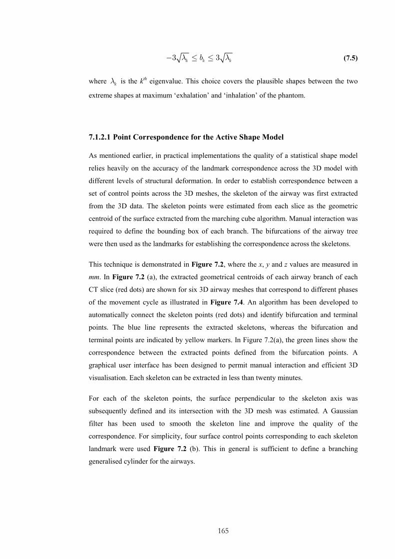
165
3 3k k kbλ λ− ≤ ≤ (7.5)
where kλ is the kth eigenvalue. This choice covers the plausible shapes between the two
extreme shapes at maximum ‘exhalation’ and ‘inhalation’ of the phantom.
7.1.2.1 Point Correspondence for the Active Shape Model
As mentioned earlier, in practical implementations the quality of a statistical shape model
relies heavily on the accuracy of the landmark correspondence across the 3D model with
different levels of structural deformation. In order to establish correspondence between a
set of control points across the 3D meshes, the skeleton of the airway was first extracted
from the 3D data. The skeleton points were estimated from each slice as the geometric
centroid of the surface extracted from the marching cube algorithm. Manual interaction was
required to define the bounding box of each branch. The bifurcations of the airway tree
were then used as the landmarks for establishing the correspondence across the skeletons.
This technique is demonstrated in Figure 7.2, where the x, y and z values are measured in
mm. In Figure 7.2 (a), the extracted geometrical centroids of each airway branch of each
CT slice (red dots) are shown for six 3D airway meshes that correspond to different phases
of the movement cycle as illustrated in Figure 7.4. An algorithm has been developed to
automatically connect the skeleton points (red dots) and identify bifurcation and terminal
points. The blue line represents the extracted skeletons, whereas the bifurcation and
terminal points are indicated by yellow markers. In Figure 7.2(a), the green lines show the
correspondence between the extracted points defined from the bifurcation points. A
graphical user interface has been designed to permit manual interaction and efficient 3D
visualisation. Each skeleton can be extracted in less than twenty minutes.
For each of the skeleton points, the surface perpendicular to the skeleton axis was
subsequently defined and its intersection with the 3D mesh was estimated. A Gaussian
filter has been used to smooth the skeleton line and improve the quality of the
correspondence. For simplicity, four surface control points corresponding to each skeleton
landmark were used Figure 7.2 (b). This in general is sufficient to define a branching
generalised cylinder for the airways.
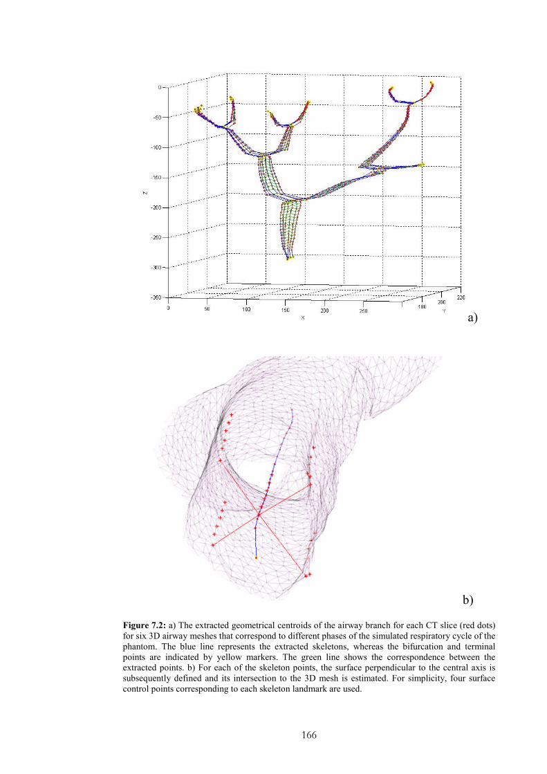
166
a)
b)
Figure 7.2: a) The extracted geometrical centroids of the airway branch for each CT slice (red dots)
for six 3D airway meshes that correspond to different phases of the simulated respiratory cycle of the
phantom. The blue line represents the extracted skeletons, whereas the bifurcation and terminal
points are indicated by yellow markers. The green line shows the correspondence between the
extracted points. b) For each of the skeleton points, the surface perpendicular to the central axis is
subsequently defined and its intersection to the 3D mesh is estimated. For simplicity, four surface
control points corresponding to each skeleton landmark are used.
167
7.1.3 Mesh Warping with Radial Basis Functions
The application of ASM to the skeleton and surface control points results in intermediate,
deformed airway structures. To generate a smooth 3D mesh of the airways, Radial Basis
Functions (RBFs) are used. An RBF is a continuous function, of at least 1C continuity that
provides smooth, controllable deformation. It maps each control point in one domain to the
corresponding control point in the other with interpolation of the mapping at intermediate
points. An RBF spatial transformation in d dimensions, denoted ( ),T x y , is composed of
1, ,k d= … mapping functions [176], such that:
( ) ( ) ( ) ( )[ ]1, , , ,
k dT x f x f x f x=
… … (7.6)
With RBFs, each of the mapping functions can be decomposed into a global component
and a local component, and this decomposition enables a family of transformations to be
defined where the influence of each control point can be determined. Given n pairs of
corresponding control points, each of the k mapping functions of the RBF takes the
following form:
( ) ( ) ( )1
n
k mk ik i
i
f x P x A g r=
= +∑ (7.7)
where ( ), ,x x y z=
, ( )mkP x
, is a polynomial of degree m , ( )
ig r is a radial basis
function, ir denotes the Euclidean norm defined by
i ir x x= −
(7.8)
and iA corresponds to the ith-column of the parameter array W . It is worth noting that the
polynomial term has been omitted and ( )ig r is a linear radial basis function that expresses
the contribution of each control point on the original vertex.
In the 3D case represented in this study and ignoring the polynomial term of Equation 7.7,
the RBF transformation is determined by n coefficients in each dimension. The
coefficients of the function ( )kf x are determined by constraining ( )
kf x to satisfy the
interpolation conditions and solving the following linear system of equations:
168
1W G Y−= (7.9)
where ( ) ( ), ijG i j g r= , and Y is a matrix with the deformed points. Intuitively, ( )ijg r
measures the effect of the jth control point on the transformation at the i
th control point. The
above equation is typically solved by using Singular Value Decomposition (SVD) and the
new position of each vertex is then calculated from Equation 7.7. During calculation, since
the vertices have been changed the normals also need to be recalculated. In this study, the
normals for each rendered scene are implicitly estimated as part of the registration
procedure.
7.1.4 A pq-based Similarity Measure
The basic principle of constructing a similarity measure for the 2D/3D registration is based
on the original pq-based framework suggested in Chapter 4. In this technique, surface
normals of the video endoscopic image are extracted by using a linear shape-from-shading
algorithm, which exploits the unique endoscopic camera/lighting special configuration.
During registration, these vectors are matched to the surface normals of the 3D model with
its deformation controlled by the ASM and axial camera rotation. The similarity measure of
the two images was determined by evaluating the dot product ϕ of the corresponding pq-
vectors. By incorporating the mean angular differences and the associated standard
deviations σ , the following similarity function is used:
( ) ( )( )1
31w w DS nϕ σ ϕ
− = ⋅ − ⋅ ∑∑ ∑∑ (7.10)
where 3Dn is the surface normals derived from the 3D model and wϕ stands for the
weighted dot product. With this scheme, neither the lighting parameters nor the other
rendering parameters need to be adjusted during registration. The similarity measure is
weighted according to the 3D model surface vectors, such that it is relatively immune to
texture discrepancies that are common to the endoscopic images. For optimising the above
similarity measure, the Simplex algorithm by Nelder and Mead was used [177].

169
7.2 Incorporating EM Tracking Devices
In previous chapters, we have emphasised the fact that an EM tracker reports only the
position and orientation of the bronchoscope camera in relation to fixed, world coordinates.
For this reason, direct mapping of the EM tracking measurements to the static preoperative
CT images is not appropriate, and its practical use must be considered in relation to both
the deformation of the airways and the global motion of the patient. In the last chapter, it
has been demonstrated how to utilise the measurements of a positional sensor attached on
the patient chest to decouple global and respiratory motion. Subsequently, this information
can be used to remove the global motion component from the EM data. In this chapter,
ASM is used to model the motion of the airways during respiration.
The next step of this approach is to transform the EM data from the EM coordinate system
to the preoperative image coordinate system. To this end, three landmarks have been added
to the phantom such that can be accurately identified in the pre-operative scans. By
marking them with the tip of the EM tracker, their positions can be determined in the EM
tracker coordinate system. In a real-case scenario, three or more reliable landmarks should
be identified during a bronchocopy session and then matched to the pre-operative images.
Subsequently, a rigid transformation between the two coordinate systems can be
determined based on a close-form solution. In this method, a rigid-body transformation is
expressed as a combination of a rotation R and a translation t . So a point Ar from A
coordinate system is transformed to Br in B coordinate system by the following formula:
B AB A ABr R r t= + (7.11)
Consequently, a rigid-body registration seeks the values of R and t that minimize the
mean square error given 3D point correspondences iA
r and iB
r , i.e.,
( )2
,1
mini i
N
B AR t
i
r R r t=
− ⋅ +∑ (7.12)
In the work by Horn et al. [169, 170] showed that it is possible to reformulate the problem
to decouple the computation of R and t and solve it with a closed form solution. This can
be done by referring the coordinates to the respective centroids of each point set, leading to
the minimization of the following equation:

170
( )2
,1
mini i
N
B AR t
i
r R r=
′ ′− ⋅∑ (7.13)
1
1i i i
N
A A A
j
r r rN =
′ ′= − ∑ (7.14)
1
1i i i
N
B B B
j
r r rN =
′ = − ∑ (7.15)
Subsequently, the translation is given by the difference of centroids:
1 1
1 1i i
N N
B A
j j
t r R rN N= =
= −∑ ∑ (7.16)
Subsequently, the rotation can be represented by either orthonormal matrices or quaternions
[169, 170]. However, quaternions offer a more stable solution than orthonormal matrices as
for the latter the orthonormality contraint should be maintained in each step. Once the
quaternion representation has been adopted, the solution is obtained by the most positive
eigenvalue of the matrix N .
xx yy zz yz zy zx xz xy yx
yz zy xx yy zz xy yx zx xz
zx xz xy yx xx yy zz yz zy
xy yx zx xz yz zy xx yy zz
S S S S S S S S S
S S S S S S S S SN
S S S S S S S S S
S S S S S S S S S
+ + − − − − − − + +
= − + − + − − − + − − − +
(7.17)
where the elements of the matrix S are estimated as:
1i i
n
xx B A
i
S x x=
′ ′= ⋅∑ and 1
i i
n
xy B A
i
S x y=
′ ′= ⋅∑ (7.18)
7.3 Incorporating Temporal Tracking
The use of ASM allows the incorporation of deformable modelling into the registration
process. This enables the efficient use of EM tracking data to further improve the
registration accuracy. In Chapter 5, it has been emphasised that both image-based and EM
tracking techniques have certain limitations. A probabilistic tracking framework based on
171
the Condensation algorithm is used to allow the use of multi-modal probability
distributions, which is essential to track the camera position under airway deformation and
image artefacts. This framework provides an effective way of combining the results from
pq-space registration with EM tracking to enhance the robustness of the non-rigid
registration processing. In essence, temporal tracking uses a prediction model to evolve a
number of particles and a measurement model to assign a weight to each particle.
Subsequently, by evaluating the given moments of the state density, it estimates the most
probable state.
It should be noted, however, the observation model of Chapter 5 was based only on the
image-based registration results. In this chapter, the observation/measurement model needs
to combine both the EM tracker measurements and the image-based registration results.
Generally, the observation density ( )|t tp z x defines the likelihood that a state tx causes
the measurement tz . This is typically achieved by assuming that the measurements are
statistically independent both mutually and with respect to the process model. Furthermore,
both the EM tracker and the image-based registration measurements are imprecise. In this
study, the uncertainty is quantified with a Gaussian probability density function
( )0,p N σ∼ , where the variance σ , depends on the reliability of the different sensors
measurements. The observation density for a particular state is estimated by integrating
over the space of sensors measurements:
( )| mtt t z
m
p z x p=∑ (7.19)
The state of the system has been defined as the 6 DoF pose of the camera. For the process
model, a second order auto-regressive model was used to describe the motion of the
endoscopic camera. A detailed description of this model is provided in Section 5.3.
Training of this model is based on the algorithms also described in Chapter 5 and the
training sequences have been constructed based on the EM tracking data. since EM tracking
data are available only for 5 out of 6 DoF, the last degree-of-freedom was tracked
independently.

172
7.4 Experimental Design
Figure 7.3: The bronchoscope navigation paths involved in this study, where the camera travels
from the right branch (frame-9780) to the trachea (frame-10845) and then continues to the left
branch (frame-12501).
In order to assess the registration accuracy of the proposed algorithm, a dynamic phantom
was constructed to imitate the airway deformation during respiration. An optical
bronchoscope has been used to navigate inside the phantom tree. Figure 7.3 illustrates the
path that has been followed during the experiment. The bronchoscope travels from the end
of the right branch back to the trachea and then continues to the left branch. A 5DoF EM
tracker was inserted in the biopsy channel to facilitate the 2D/3D registration. The ground
truth data for the non-rigid parameters of the 2D/3D registration has been provided from an
EM sensor attached on the phantom to monitor the deformation phase during navigation.
To validate the accuracy of the non-rigid 2D/3D registration technique two experiments
have been designed. Firstly, the 5DoF’s of the rigid registration that define the position and
two of the rotation angles have been directly recovered from the 5DoF EM tracker. The
sixth DoF, which defines the rotation of the camera around its axis, as well as the
deformation parameters have been recovered by optimising a pq-based similarity measure.

173
Quantitative results have been provided for the recovered deformation parameters in
Section 7.5.4. This section also provides with qualitative results of the overall accuracy of
the non-rigid 2D/3D registration.
A second experiment has been designed to show the effectiveness of the temporal tracking.
Temporal tracking has been applied to only the rigid motion of the camera and not to the
deformation parameters. The EM tracking data have not been used directly to define the
pose of the camera, but they were combined probabilistically with the image-based
registration results to provide the optimal pose.
7.4.1 Video Preprocessing
Prior to 2D/3D registration, pre-processing of the videos was necessary in order to alleviate
the effects of interlacing, lens distortion, and image artefact. Preprocessing of the
endoscopic frames is similar to Section 4.3.5. De-interlacing can be achieved by separating
odd/even scan lines, which is particularly important to minimise the comb effect during fast
advancement or retraction of the bronchoscope. To correct for barrel distortion due to the
wide angle bronchoscope camera used, the camera model suggested by Heikkil, which
includes both radial and tangential distortion of the video image, was used. The
initialization of the calibration parameters follows the work by Zhang et al. Finally, to
improve the SNR of the video image, a structure adaptive anisotropic filter was used [136].
The method uses a local orientation and anisotropic measure to control the shape and extent
of the filter kernel and thus ensures that salient image features are well preserved whilst
removing image artefacts. The method generally provides a smoother optimisation
landscape, and brings improved convergence of the 2D/3D registration algorithm.
7.4.2 Phantom Setup
In this study, the airway phantom was made of silicon rubber and painted with acrylics. The
inner surface was coated with silicon-rubber mixed with acrylic to give it a textured and
specular finish that is similar to the bronchial lumen. The phantom surface was finished
with red colour splashes to imitate the blood and texture discrepancies during a
bronchoscope examination. The distal ends of the airway-phantom have been fixed and a
balloon is located below the main bifurcation to simulate respiratory-induced airway

174
deformation as shown in Figure 7.4. The navigation paths used for validation are also
indicated in Figure 7.3. The extent of the airway motion is regulated by a valve controlling
the amount of air in the balloon. The tomographic model of the phantom was scanned with
a Siemens Somaton Volume Zoom 4-channel multi-detector CT scanner with a slice
thickness of 1 mm and in-plane resolution of 1 mm. A total of six CT volumes were
acquired at different stages of the motion cycle.
Figure 7.4: Illustrations of the phantom setup during two different deformation stages. a) The
maximum level of deformation is achieved when the balloon is full of air, and b) shows the resting
state when the balloon is empty.
a)
b)

175
7.4.3 Ground Truth Data
To track the pose of the bronchoscope camera, an NDI (Northern Digital Inc, Ontario)
Aurora EM tracker was used. The Aurora system is particularly suited for tracking flexible
endoscopes during minimally invasive intervention. This typically employs a single coil
sensor due to size restrictions imposed by the biopsy channel. Having only a single coil,
however, the sensor is limited to reporting position and direction only (i.e. 5 DoF with
unknown axial rotation). The working volume of the Aurora system is within 500mm cube
located 50mm from the field generator. In an environment that is free from Electro-
magnetic interference, the Aurora has a static positional accuracy of 0.9-1.7mm and an
orientation accuracy of 0.5 degrees.
In order to obtain the ground truth deformation data, a real-time, 6 DoF EM tracker tool
was used to track the deformation of the balloon so that the deformation of the phantom
airway can be indexed back to the 3D CT data. An Olympus bronchoscope (Olympus BF
Type, with a field of view 120°) operating in PAL recording mode (25fps) was used to
capture the 2D bronchoscope video.
In this study, the ground truth data used was provided by the 6-DoF EM tracker attached to
the balloon controlling the level of simulated respiratory motion. This permits the direct
association of the deformation of the airway phantom during bronchoscope examination
with the exact 3D geometrical shape captured by CT. The projections of the deformation as
mapped onto the principal axes defined by the ASM were used in this study to provide a
quantitative measure of the effectiveness of the registration process, i.e.,
( ) 1
1T
r r rb M p p p−
= ⋅ ⋅ ⋅
(7.20)
where rp is the eigenvector that corresponds to the point rs of the 3D mesh that is nearest
to the position of the 6-DoF EM tracker, and Mis the vector between these two points.
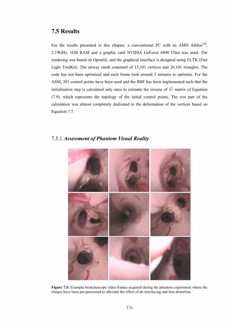
176
7.5 Results
For the results presented in this chapter, a conventional PC with an AMD AthlonTM,
2.19GHz, 1GB RAM and a graphic card NVIDIA GeForce 6800 Ultra was used. The
rendering was based on OpenGL and the graphical interface is designed using FLTK (Fast
Light ToolKit). The airway mesh consisted of 13,101 vertices and 26,101 triangles. The
code has not been optimised and each frame took around 3 minutes to optimise. For the
ASM, 301 control points have been used and the RBF has been implemented such that the
initialisation step is calculated only once to estimate the inverse of G matrix of Equation
(7.9), which represents the topology of the initial control points. The rest part of the
calculation was almost completely dedicated to the deformation of the vertices based on
Equation 7.7.
7.5.1 Assessment of Phantom Visual Reality
Figure 7.5: Example bronchoscope video frames acquired during the phantom experiment where the
images have been pre-processed to alleviate the effect of de-interlacing and lens distortion.

177
To demonstrate the general visual appearance of the phantom airway model, Figure 7.5
illustrates 9 example frames of the video sequence after pre-processing, which includes de-
interlacing, lens distortion, and anisotropic smoothing. Red stains have been added on the
inside phantom walls to imitate vessels and texture discrepancies. The accuracy of the
registration scheme does not degrade in the parts of the phantom where these features are
eminent. This indicates that the registration algorithm is relatively immune to texture
discrepancies as it has been also demonstrated in Chapter 4.
7.5.2 Phantom Deformability
Figure 7.6: The normalised mesh displacement between successive deformation stages of the
phantom.
To demonstrate the amount of deformation introduced, the normalised mesh displacement
map at five different deformation positions of the phantom are shown in Figure 7.6,
illustrating the non-linear, localised deformation at different branches of the airway. By
reference to the navigation paths shown in Figure 7.3, it is evident that we have chosen the
most deformed part of the airway phantom for the validation purpose.
In this study, the main purpose of the phantom design is to assess the extent of free-form
deformation and its effect on the accuracy of 2D/3D registration. It should be noted that the
phantom is not a complete representation of the airway structure and its physiological
response. The air flow patterns and the force distribution on the airway conduits are patient-

178
specific and they vary significantly across different subjects [178]. Since the ASM model is
to be constructed on a patient-specific basis, the proposed phantom validation framework
should provide a good indication of the achievable accuracy of the algorithm for in vivo
applications.
7.5.3 Modelling of the Airways Respiratory Motion
Figure 7.7: The result of applying the ASM to the reconstructed 3D volumes, illustrating the warped
3D mesh by using the RBF along the first principal mode of the shape variation. The red, green, and
blue meshes correspond to varying 13 λ− , 0, and 13 λ+ from the mean shape.
Table 7.1 shows the total modelling error associated with each eigenvalue. It is evident that
the first principal component captures most of the airway deformation, which means that
even by varying the first mode alone, most of the structural deformation as reconstructed by
RBF can be used to control the subsequent 2D/3D registration process. This was also
convenient for validating the deformation parameters with ground truth data derived from
one sensor attached on the phantom. However, further investigation needs to decide
whether in clinical practice more parameters should be taken into consideration to
adequately model the deformation of an in vivo tracheo-bronchial tree during respiration.
This is not expected to change the overall accuracy of the suggested non-rigid registration
framework but it will considerably increase the time of the optimisation convergence.

179
The result of applying the ASM to the reconstructed 3D volumes are also shown in Figure
7.7, illustrating the warped 3D mesh by using the RBF along the first principal mode of the
shape variation in the sagittal, coronal and axial views. The red, green, and blue meshes
correspond to varying 13 λ− , 0, and 13 λ+ from the mean shape, respectively. These
are the extreme values of the allowable shape domain. The quality of the ASM depends on
the extraction of correspondence features between the avaluable set of 3D CT data. The
overall results indicate that the ASM adequately captures the variability induced in the
phantom airways. Most, errors are consentrated in the bifurcation points because the angle
between the skeleton and the perpendicular plane at these points is not well defined.
EigenValues in Descending order 1st 2nd 3rd 4th 5th 6th
Error in mm 4.3542 0.7723 0.6170 0.1482 0.055 0.0
Error in percentage (%) of the phantom diameter 10.88 1.93 1.54 0.3706 0.1392 0.0
Table 7.1: Modelling error associated with omitting each eigenvalue individually
7.5.4 Accuracy of Deformable 2D/3D Registration
The performance of the proposed registration algorithm by using the EM tracking data
combined with the deformable model as determined by ASM can be examined in Figure
7.8. In this figure, the top row is the bronchoscope view of the phantom airway, whereas
the middle row illustrates the corresponding view of the 3D model determined by the 5
DoF catheter tip EM tracker. Significant mis-registration is evident due to the unknown
rotation and airway deformation. It is evident that the position of the camera changes
rapidly due to the respiratory motion in the world coordinates, and a direct use of the EM
data can result in initial camera position located completely outside of the bronchial tree.
The result of applying the proposed registration algorithm is shown in the bottom row of
Figure 7.8, demonstrating the visual accuracy of the method. The frames shown have been
acquired at different parts of the tracheo-bronchial tree as it is depicted in Figure 7.3.
Generally, the algorithm performs better when prominent features are apparent in the
endoscopic images. Such features can visually describe bifurcations or protuberances on
the phantom airway walls due to simulated lesions or natural surface folding. The larger
inaccuracies occur when the camera is facing the wall and the light diffuse in such a way
that it is not able to distinguish any surface details.

180
In order to provide a detailed quantitative validation of the method, Figure 7.9 illustrates
the recovered deformation as projected onto the first principal axis of the ASM model. In
other words, this reflects how parameter 1b controls the shape of the mesh based on
Equation (7.5). The corresponding ground truth value as determined by the 6 DoF EM
tracker from Equation (7.21) is also provided for comparison. It is evident that the
reconstruction result followed the ground truth reasonably well. Further details of the error
analysis are illustrated in Figure 7.10, which provides a Bland-Altman plot of the errors of
the recovered deformation as compared to the ground truth. The Bland-Altman plot reveals
how well two datasets agree with each other.
Figure 7.8: The performance of the proposed registration algorithm by using the EM tracking data
combined with the deformable model as determined by ASM. Left-column: the bronchoscope view
of the phantom airway; Mid-column: the corresponding view of the 3D model determined by the 5
DoF catheter tip EM tracker where significant mis-registration is evident due to unknown rotation
and airway deformation; Right-column: the result of applying the proposed registration algorithm

181
demonstrating the visual accuracy of the method.
Figure 7.9: The recovered deformation as projected onto the first principal axis of the ASM model
where the corresponding ground truth value (dotted curve) as determined by the 6 DoF EM tracker
from Equation (7.21) is provided for comparison.
0 1 2 3 4 5 6 7 8 9
-10
-5
0
5
10
Bland-Altman Plot
Average of GT and NR
Difference between GT and NR in mm
Figure 7.10: Bland-Altman plot of the non-rigid registration results as compared
to the ground truth.
-2.1
-1.4
-0.7
0
0.7
1.4
10750 10950 11150 11350 11550 11750 11950 12150 12350 12550number of frames
Ground Truth
Non-Rigid Registration

182
7.5.5 Temporal Tracking
0
10
20
30
40
50
60
0 100 200 300 400 500 600 700 800
Frame Number
Distance (mm)
EM Tracking Data
Condensation
Figure 7.11: Euclidean distance between the first and subsequent camera position as it has been
predicted from the Condensation algorithm with relation to the EM tracking data.
Figure 7.11 illustrates the results by applying the Condensation algorithm to a video
segment as compared to the ground truth data recovered from the EM data. The results
show that this scheme was effective because it has the ability to correct errors and failures
of both techniques. It is able to recover even if either of them fails. Tracking of the camera
based only on the EM tracker device’s results in errors due to inaccuracies in the initial
coordinate transformation. This is more prominent when the airways deform dynamically
due to the bronchoscope itself. Currently, the suggested registration scheme cannot recover
these deformation parameters. Subsequently, temporal tracking improves the overall
accuracy by relying on both measurements.
7.6 Discussions and Conclusions
In this chapter, we have proposed a deformable 2D/3D registration framework based on
ASM. Despite the prevalence of tissue deformation in most surgical navigation and
planning applications, its incorporation into the 2D/3D registration framework has been
limited. This is due to the large degrees-of-freedom involved in the registration parameters,
which make a stable implementation of the algorithm difficult.

183
The recent advance of miniaturised catheter tip EM trackers has greatly simplified the
2D/3D registration process. For rigid registration, existing 5 DoF EM tracker inserted into
the biopsy channel of the endoscope can provide much improved results as the remaining 1
DoF is relatively easy to optimise. For deformable airways, however, existing research has
shown that complex deformation of the anatomical structure still represents a major
problem to the registration process despite the use of the catheter tip EM tracker [75]. In
this case, direct application of local deformation to the 3D structural mesh to match to that
of the bronchoscope video is computationally impractical due to the large number of
control points involved. Furthermore, issues such as mesh folding also need to be carefully
addressed. Although it is possible to use the finite element model to provide bio-
mechanically plausible model to define airway deformation, its practical implementation
can be difficult due to the general lack of detailed tissue mechanical property, as well as the
prohibitive computational cost involved.
In this study, we have demonstrated that the use of ASM provides a simple yet effective
framework for a compact representation of the airway deformation. This allows
deformation to be modelled by the limited principal modes of variation such that
conventional optimisation processes can be effectively applied. Statistical shape models
and PDMs in particular, provide an effective means of capturing statistically plausible
variations of the shape of the object. The ASM combines a model-based approach similar
to template models that allow for large variability with a prior knowledge incorporated
through a number of previous observations. It has a number of advantages for its use in a
non-rigid 2D/3D registration framework. The method describes both typical shape and
intrinsic deformation and the motion variability is accommodated through prior knowledge
incorporated through the 3D data. Therefore, they can effectively model the deformation of
the structure even though the motion mechanisms are not sufficiently understood, or too
complex to derive. Furthermore, they are specific to the class of motion they represent, and
hence can be implemented in a subject specific manner.
It should be noted, however, that the effectiveness of the method depends on the ability of
the 3D models in capturing possible structural deformations during video bronchoscope
examination. For the phantom experiment presented in this chapter, we have used CT to
provide the structural information of the airways. This, however, may not be suitable for
patient studies as the capture of airway deformation at different phases of the respiratory
cycle for constructing the ASM model can involve significant ionising radiation. A more
practical choice would be to use the recent developments of MRI that permits the
visualisation of the lung parenchyma and airways during normal physiological motion [51].
184
The combination of respiratory navigator echoes will allow the imaging of the intra-
thoracic tree at different stages of the respiratory motion, and therefore the construction of a
complete deformable model of the airways on a subject-specific basis.
It is also important to note that with the proposed registration framework, the global motion
of the patient must be monitored during bronchoscope examination such that it is removed
from the catheter-tip EM tracking data for localising the catheter tip in relation to the CT
scan volume. This is an issue not encountered in the traditional image registration
framework as global motion of the patient will result in a synchronous movement of the
bronchoscope and the airways. This problem, however, can be addressed by tracking
externally the position and orientation of the patient during bronchoscope examination
[154]. The advantage of the proposed method is that it provides a practical way of handling
airway deformation and continuation of the registration process when extreme breathing
patterns and artefacts caused by mucosa, bubbles, bleeding are encountered. In a typical
examination, these effects account for 20-30% of the procedure and they can reach almost
100% in extreme cases, such as profuse haemoptysis. These effects interleave during
common bronchoscope procedures, thus providing only short video sequences where
image-based registration approaches are successful. When the registration fails it is not
trivial to recover the camera position and re-initialise the algorithm. EM tracking, however,
is much more immune to these problems [154]. The use of 5 DoF catheter tip EM tracker
combined ASM can provide a closer approximation of the camera pose such that the exact
solution to the problem can be limited to a localised search space. Patient data also
indicates that at the bifurcation/turning points, a rigid model is relatively difficult to
smoothly follow the video frames, since the pre-operative and intra-operative 3D structures
may not be in correspondence.
In terms of localised airway deformation, one additional problem that deserves
consideration is that in typical tomographic imaging the patient is in a supine position,
whereas in bronchoscope examinations the patient typically adopts an upright posture. It is
feasible that the deformation of the intra-thoracic airways due to the gravity effect may be
different due to the variation in pose. This, however, is a problem that is encountered by all
2D/3D registration techniques.
It should also be noted, that the success of ASM depends on the number and quality of
correspondent landmarks across the observable shapes. A simplistic method was used to
extract the skeleton of the tracheo-bronchial tree and subsequently correspondence was
established based on the matching of the bifurcation points. The identification of optimal
185
control points for ASM for complex topological shapes, however, is a significant challenge
[179].
Since the ASM is based on landmark correspondence, an effective way of smoothly
interpolating the mesh points with regard to the motion of the control points is necessary.
RBFs have been used for a number of reasons. Firstly, the distribution of the control points
can be both sparse and irregular. RBF provides an easily controllable behaviour that can be
tailored to meet specific requirements. It may be purely deformable, or contain some forms
of linear component to allow for both localised and global deformations [176]. Other
techniques such as the one presented by Garrity et al. [95] uses NURBS based surface
representation are also possible for creating the dynamic model of the airway. The actual
computational complexity for estimating each new vertex with RBFs is ( )O nN , where n is
the number of control points and N is the number of vertices. The solution of the equation
system in the pre-processing step requires an additional 3( )O n . Here we calculate the SVD
only at the initialisation stage of the algorithm since the topology of the points does not
change. Therefore, the time required depends mainly on the number of vertices of the 3D
model, which are usually much larger than the number of control points. These time
requirements can also be optimised. For example, the mesh can be deformed only locally
since the bronchoscope only provides a localised view of the airways. Other improvements
such as to bind locally the radial basis functions and use of parallel processing can also be
introduced [176].
In conclusion, we have developed a non-rigid 2D/3D registration framework that models
the respiratory motion of the intra-thoracic tree which incorporates the EM tracking data for
improved robustness and accuracy. ASM has been used to capture the intrinsic variability
of the airways across different phases of the respiratory motion and it also constrains the
motion they represent to be specific to the subject studied. This allows the subsequent non-
rigid registration implemented in a much reduced dimensional space, and thus greatly
simplifies the 2D/3D registration procedure. The detailed phantom validation of the method
in this study demonstrates the potential clinical value of the technique.

186
Chapter 8
Conclusions and Future Work
n this thesis, we have developed a registration framework for constructing subject-
specific simulation models for virtual bronchoscopy. By fusing real bronchoscopy video
with 3D tomographic data of the same patient, it is possible to generate photorealistic
models that allow high fidelity, patient specific bronchoscope simulation. In order to match
video bronchoscope images to the geometry extracted from 3D reconstructions of the
bronchi, robust registration techniques have to be developed. This is a challenging problem
as it implies 2D/3D registration with certain degrees of deformation and different
physiological responses. In this thesis, we have proposed a new pq-space based 2D/3D
registration method for camera pose estimation in endoscope tracking. The proposed
technique involves the extraction of surface normals for each pixel of the video images by
using a linear local shape-from-shading algorithm derived from the unique camera/lighting
constrains of the endoscopes. We demonstrate how to use the derived pq-space distribution
to match to that of the 3D tomographic model. The registration algorithm is further
enhanced by introducing temporal constrains based on particle filtering. For motion
prediction, a second-order auto-regressive model has been used to characterize camera
motion in a bounded lumen as encountered in bronchoscope examination. The proposed
method provides a systematic learning procedure with modular training from ground truth
data such that information from different subjects are integrated for creating a dynamic
model that accommodates the learnt behaviour. To cater for airway deformation, an active
shape model (ASM) driven 2D/3D registration has been proposed, which captures the
intrinsic variability of the tracheo-bronchial tree during breathing and it is specific to the
class of motion it represents. The method reduces the number of parameters that control the
deformation, and thus greatly simplifies the optimisation procedure. The method also
exploits the recent development of 5 DoF miniaturised catheter tip electro-magnetic
I

187
trackers such that the position and orientation of the bronchoscope can be accurately
determined under dis-occlusion and bleeding. The accuracy of the proposed method has
been assessed by using both a specially constructed airway phantom with an electro-
magnetic tracker, and in vivo patient data. The original contribution of this thesis includes
the following aspects.
8.1 Main contributions of the thesis
8.1.1 A novel pq-space based registration scheme
A novel similarity measure has been introduced in Chapter 4 based on the angular
differences between pq-vectors derived from the video image and the 3D model. Surface
information is extracted from a robust linear shape-from-shading technique that exploits the
camera and lighting configuration of bronchoscope. These pq-vectors are used to match to
the normals specified from the 3D model. For the similarity function developed, it also
involves a weighting factor that accounts for texture variations of the tracheo-bronchial
tree, which are absent from the 3D CT model. The main advantages of the proposed
technique are that there is no need to adjust the illumination conditions in 3D rendering and
the method does not require feature extraction and matching. The method is also superior to
the alternative approach of surface-to-surface registration. This is because surface
reconstruction from pq-vectors requires an integration step, which is error prone. The
technique was validated with phantom data with known ground truth. In vivo bronchoscope
data has also been used to assess the practical value and potential pitfalls of the technique.
It has been shown that handling large tissue deformation and occlusion artefacts are major
obstacles of the proposed method when applied to in vivo bronchoscope sequences. To this
end, temporal information must be integrated into the proposed registration framework for
it to be practically useful.
188
8.1.2 Incorporation of temporal constrains based on particle filtering
The incorporation of temporal constraints is based on particle filtering in this thesis. A
probabilistic framework has been developed in Chapter 5 to utilise the inherent in
bronchoscope camera motion between successive video frames to improve the accuracy of
the 2D/3D registration algorithm. Although the concept of particle filtering itself is not
new, we have tackled the difficult problem of dynamic model building and modular
learning. A second order autoregressive (ARG) model has been used to evolve the
underlying model through time, and the method weights the propagated hypotheses for
accurate pose estimation. A systematic training procedure has been developed to tune the
parameters of the ARG model based on modular learning. There are two main advantages
of the probabilistic tracking algorithm suggested. Firstly, there are no restrictions on the
measurement models used and the distribution of error sources. This allows the handling of
non-linear dynamics during endoscope navigation. Secondly, modular training facilitates
the incorporation of multiple sequences from different patients. In this way a generic
motion prediction model can be developed.
8.1.3 Miniaturised EM tracking and motion decoupling
The challenges involved in incorporating EM trackers into bronchoscope navigation have
been investigated in Chapter 6. Although, EM tracking devices have the potential to
enhance real-time 2D/3D registration, ferromagnetic interference and tissue deformation
can limit their practical accuracy in clinical environments. For the proposed 2D/3D
registration framework, it is also necessary to decouple local deformation from global
motion. To this end, we have developed a new motion decoupling scheme based on
principal component analysis to identify the variation of the EM signal due to respiration
and global patient movements. The method has also been used to identify extreme
breathing patterns so that these segments can be treated separately during 2D/3D
registration.
8.1.4 Deformation modelling based on statistical shape models
Conceptually, the development of statistical shape models for deformation modelling
during 2D/3D registration is the most significant part of the thesis. Currently, most of

189
2D/3D registration methods are based on rigid or affine models and the high degrees of
freedom involved in free-form deformation models are both technically and
computationally prohibitive. In Chapter 7, we have used statistical shape modelling
combined with EM tracking to significantly reduce the number of degrees-of-freedom
involved in the registration process. In this thesis, deformation modelling has been
implemented by extracting the skeleton of the tracheo-bronchial tree and establishing
surface point correspondence based on bifurcation points. Radial Basis Functions (RBFs)
have been used to warp the mesh in intermediate positions. Motion compensation is
attained with the recovery of the deformation of the tracheo-bronchial tree along with the
pose estimation. In this way, EM tracking data can be directly applied to guide the
registration process. We have shown that for the phantom model that involves extensive
non-linear deformation, the degrees of freedom has been reduced to only two – one for the
unknown rotation of the camera and the other for the principle mode of variation describing
the deformation of the airways. For in vivo data, the principle modes of variation are
expected to be higher. Nevertheless, this is likely to be limited to only a few rather than the
otherwise thousands of DoFs.
8.2 Discussion and Conclusions
Despite the achievements made, there are several major improvements that can be made for
future research. In Chapter 4, we suggested a pq-space similarity measure. However, by the
nature of the shape-from-shading algorithms, specularities and inter-reflections have been
ignored. In bronchoscopic images, strong reflections are common due to mucosa and
surface properties of the lumen. Conventional shape-from-shading techniques can mistake
the presence of local specularities as high curvature surface features [180]. Although we
have directly used pq distribution during registration to minimise this effect, its explicit
consideration needs to be taken into account. For human observers, we in fact rely on
specular reflection to provide an additional visual cue for the 3D surface, such information
can potentially be utilised to further enhance the 3D structural reconstruction process.
In practice, the detection of specular highlights can be achieved by a dichromatic model but
it is also possible to factor in the reflectance properties into the shape-from-shading
algorithm itself. There are several ways in which surface reflectance properties can be
approximated. If a surface is too difficult to be described by a particular model then a
general approach can be used to acquire empirical estimates of the Bidirectional

190
Reflectance Distribution Function (BRDF). This is an expensive and time consuming
process because BRDF is described from a large number of degrees of freedom. But
empirical and physical-based methods can be used to simplify its derivation. In
bronchoscope procedures, the light coincides with the viewer and this can simplify the
estimation of the surface properties.
Another issue that deserves extensive future research is the effective handling of local
minima of the registration process. Although the use of global optimisation techniques can
help the overall consistency of the registration process, a systematic approach needs to be
adopted to combine the construction of the similarity measure with the subsequent
optimisation landscapes. In this thesis, the construction of the similarity measure is
empirically designed but the parameters involved are not determined systematically. The
integration of temporal information partly alleviates the problem of local minima but
further investigation of using a learning based framework is necessary so that the overall
robustness of the algorithm can be further enhanced.
In this thesis, the integration of temporal information for the registration scheme is
presented. One of the major advantages of this probabilistic framework is that it
incorporates modular training. This allows the learning of the dynamic motion
characteristics of the endoscope from several training sets, so that a more representative
dynamic model can be created. However, a problem arises when more complex dynamics
involving multiple classes of motion [141]. In this work, the dynamic motion
characteristics are modelled as a second order autoregressive model. This is a versatile tool
that can impose strong constraints on the camera movements and it allows the motion to
change rapidly both in speed and in direction. However, modelling of multi-class dynamics
has yet to be fulfilled. The models developed assume that the training sequences have
similar statistical patterns, which may not be true when the endoscope camera explores
different parts of the tracheo-bronchial tree. Further investigation is required to overcome
this problem.
For the ASM used in deformation modelling, we extracted the tracheobronchial skeleton
manually in order to establish the correspondence based on the matching of the bifurcation
points. However, manual segmentation of each tracheo-bronchial branch in each slice is
tedious and time consuming. A fully automated method that incorporates structural features
such as mediality and homotopy needs to be developed. This can be particularly useful for
segmenting distal airways as consistent manual segmentation is difficult, if not impossible.
Another important issue to consider is point correspondence of the ASM model.
Furthermore, it is well-known that the success of the ASM depends on the quality of the

191
control point correspondences. In this work, we have used bifurcation landmarks to achieve
the overall structural correspondence of the 3D models. Alternatively, optimal and dense
shape correspondence can be achieved by optimising the correspondence on a parametric
space with respect to some objective functions. This implies that the tracheo-bronchial
surface should be parameterised onto a manifold with minimal distortion. These techniques
has been successfully applied in myocardium motion modelling but their application in
more complex structures, such as the airways is a challenging research issue [179].
In conclusion, we have addressed several major issues related to the construction of patient-
specific models for bronchoscope simulation. Although the technical components
developed in this thesis are only validated with airway phantom and in vivo bronchoscope
data, its applicability to general MIS simulation is evident. It must be noted that the work
presented in this thesis is part of a larger project within the Royal Society/Wolfson MIC
Laboratory where other issues related to photorealistic modelling, finite-element tissue
deformation modelling, and visual perceptual behaviour of MIS simulation are addressed.

192
Appendix A
Construction of the Projection Matrix
D/3D registration of the endoscopic video with the 3D operative data relies on the
comparison between several projections of the 3D data with the endoscopic image.
In order to obtain a correct match, a projection should be recoveverd by calibrating
the endoscopic camera and this should be applied in rendering the 3D surface
tracheobronchial data. In this paragraph, we will derive the equations that directly link the
OpenGL rendering parameters with the intrinsic parameters calculated with OpenCV
camera calibration toolbox for matalb.
Let’s assume that the focal length is defined as cf and it is described in pixels, such as
c cx cyf f fΤ = . Similarly, the principal point is also expressed in pixels as
c cx cyc c cΤ = . Let
T
c c cP X Y Z = be a point in space in the camera reference
frame and nX is its normalized pinhole image projection:
/
/
c c
n
c c
X ZX
Y Z
=
(A.1)
If we ignore lens distortion and assume skewing coefficient is equal to zero then the space
point P is projected to the pixel coordinates ,T
p p pX x y = through the camera matrix:
2

193
/0
0 /
1 0 0 1 1
c cp
p c c
Camera Matrix
X Zfcx ccxx
y fcy ccy Y Z
= ⋅
(A.2)
OpenGL, however, follows different notation, so that the coordinate axes are flipped
around the horizontal axis, as it is shown in Figure A.1.
(0,0) (nx-1,0)
(0,ny-1) (nx-1,ny-1)
(0, ny-1) (nx-1, ny-1)
(nx-1,0)
OpenGL
(0,0)
Figure A.1: In OpenGL, coordinates are flipped around the horizontal axis.
Therefore, the camera matrix takes the form:
/0
1 0 1 /
1 0 0 1 1
c cp
y p y c c
Camera Matrix
X Zfcx ccxx
n y fcy n ccy Y Z
− − = − − ⋅
(A.3)
Subsequently, the space point [ ]1 , ,T
P left top znear= corresponds to [ ]1 0,0T
pX = and
the above equation is written as:
/00
1 0 1 /
1 0 0 1 1
y y
left znearfcx ccx
n fcy n ccy top znear
− = − − ⋅
(A.4)
Similarly, the space point [ ]2 , ,T
P right bottom znear= corresponds to
2 1, 1T
p x yX n n = − − and the projection equation is written as:

194
/01
0 0 1 /
1 0 0 1 1
x
y
right znearfcx ccxn
fcy n ccy bottom znear
−
= − − ⋅
(A.5)
Based on the later two equations, we have:
ccxleft znear
fcx
ccytop znear
fcy
− = ⋅ = ⋅
and
1
1
x
y
n ccxright znear
fcx
ccy nbottom znear
fcy
− − = ⋅ − + = ⋅
(A.6)
Subsequently the OpenGL command glFrustum can be used directly to render the 3D
model.

195
Appendix B
Kalman Filtering
alman Filtering solves the problem of estimating the state of a linear stochastic
system by using measurements that are linear functions of the state. Differential
equations have provided concise mathematical models for many dynamic systems of
importance to humans. The dependent variables of the differential equations become state
variables of the dynamic system. Essential to Kalman Filtering is the development of the
state-space representation for dynamic systems described by a set of linear differential
equations.
The state, nX ∈ ℜ , of a discrete-time controlled process can be described by the linear
stochastic equation:
1 1 1k k k kX AX Bu w− − −= + + (B.1)
with a measurement mZ ∈ ℜ that is:
k k kZ HX v= + (B.2)
The n n× matrix A in the difference equation relates the state at the previous time-step to
the state at the current time-step. The n l× matrix B relates the optional control input
lu ∈ ℜ to the state X . The m m× matrix H is the measurement sensitivity matrix,
which relates the state to the measurement, kz , and kv represents the process measurement
noise. n , m and l are the dimensionalities of the state, measurement and optional input
K

196
vector, respectively. The random variables w and v represent the process and
measurement noise, correspondingly. They are assumed to be independent, white and with
normal probability distributions of covariance Q and R , respectively.
Kalman filtering can be also interpreted as a mechanism of propagating and combining
Gaussian densities. We define / 1ˆk kX − to be the a priori state estimate at step k given
knowledge of the process up to the ( )1k − step. Furthermore, /ˆk kX is the a posteriori
state estimate at step k given measurement kZ . In order to derive the equations for the
Kalman filter, we compute the a posteriori state estimate /ˆk kX as a linear combination of
the a priori estimate / 1ˆk kX − and a weighted difference between an actual measurement kZ
and a measurement prediction / 1ˆk kHX − :
( )/ / 1 / 1ˆ ˆ ˆk k k k k k kX X K Z HX− −= + − (B.3)
The n m× matrix K is called the gain or blending factor and it minimizes the a posteriori
error covariance.
The last equation elucidates that the Kalman Filter uses a form of feedback control to
estimate the process state at a particular time. The feedback is in the form of noisy
measurements. Therefore, the filter is composed of two parts: (1) the time update equations
that are responsible for propagating the current state and error covariance measurements,
and (2) the measurement update equations that implement the feedback mechanism. It is
also apparent that a number of parameters need to be calculated before the actual operation
of the filter.
These parameters are the measurement and process noise covariance, R and Q ,
respectively and the process of training is called system identification and it is about
inferring mathematical models from observations of a system. In general, it is easier to
estimate the measurement error covariance rather than the process error covariance, since
usually it is not possible to directly observe the estimated process. It is important, however,
to note that usually a relatively simple process model can produce acceptable results if the
uncertainty of the process has been tuned properly via the selection of the process noise
covariance Q . This fact highlights the significance of a successful system identification
procedure and generally applies to any probabilistic model. In this section the main
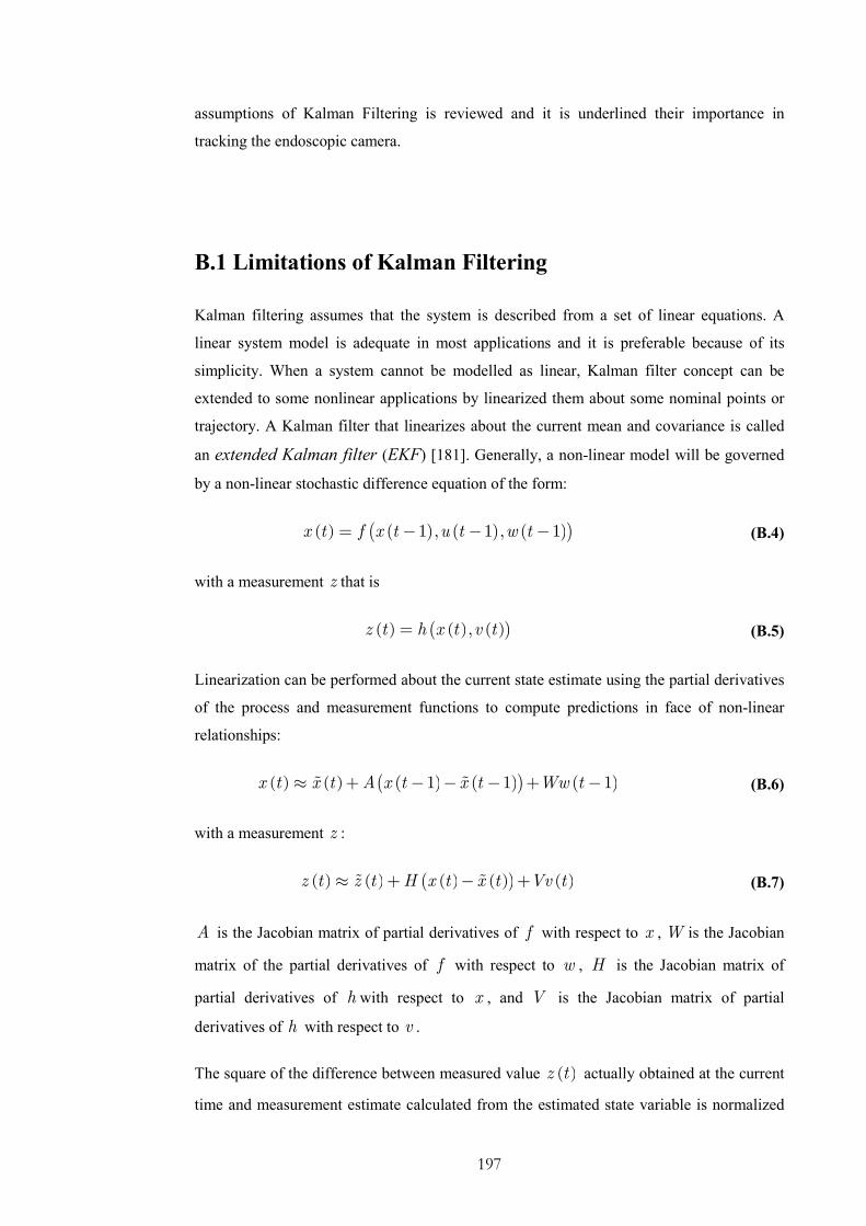
197
assumptions of Kalman Filtering is reviewed and it is underlined their importance in
tracking the endoscopic camera.
B.1 Limitations of Kalman Filtering
Kalman filtering assumes that the system is described from a set of linear equations. A
linear system model is adequate in most applications and it is preferable because of its
simplicity. When a system cannot be modelled as linear, Kalman filter concept can be
extended to some nonlinear applications by linearized them about some nominal points or
trajectory. A Kalman filter that linearizes about the current mean and covariance is called
an extended Kalman filter (EKF) [181]. Generally, a non-linear model will be governed
by a non-linear stochastic difference equation of the form:
( ) ( ) ( ) ( )( )1 , 1 , 1x t f x t u t w t= − − − (B.4)
with a measurement z that is
( ) ( ) ( )( ),z t h x t v t= (B.5)
Linearization can be performed about the current state estimate using the partial derivatives
of the process and measurement functions to compute predictions in face of non-linear
relationships:
( ) ( ) ( ) ( )( ) ( )1 1 1x t x t A x t x t Ww t≈ + − − − + − (B.6)
with a measurement z :
( ) ( ) ( ) ( )( ) ( )z t z t H x t x t Vv t≈ + − + (B.7)
A is the Jacobian matrix of partial derivatives of f with respect to x , W is the Jacobian
matrix of the partial derivatives of f with respect to w , H is the Jacobian matrix of
partial derivatives of h with respect to x , and V is the Jacobian matrix of partial
derivatives of h with respect to v .
The square of the difference between measured value ( )z t actually obtained at the current
time and measurement estimate calculated from the estimated state variable is normalized

198
with the error variance of measurements. Then the square of the difference between the
state variable ( )1x t − at the current time calculated from the state variable estimated at a
previous time and the estimated state variable ( )x t is normalized with the error covariance
matrix of ( )1x t − . The sum of these two values is the cost function, and the state variable
is estimated such that the cost function becomes the minimum. Therefore, the prediction
error takes the form of:
( ) ( ) ( )x te x t x t≡ − (B.8)
with a measurement z that is
( ) ( ) ( )z te z t z t≡ − (B.9)
This approach gives a simple and efficient algorithm to handle a nonlinear model. In
general, the extended Kalman filter is not optimal [182].
Various improvements have been introduced by iteratively updating the linearization,
starting with an initial guess. In other words, a linear Taylor approximation of the system
function is considered at the previous state estimate and that of the observation function at
the corresponding predicted position. However, convergence may not be achieved if the
initial guess is poor or if the disturbances are so large that the linearization is inadequate to
describe the system, introducing accumulated errors. The difference between the estimate
and minimum position of the cost function is amplified with the increase of the function’s
non-linearity. In the case of the cost function of EKF, past measurements are not
accumulated; instead information on the cost function is stored as the estimate. Therefore,
as the error of the estimate increases, the cost function itself contains an error. If estimation
is repeated in this status, the error gradually accumulates. Even if new measurements are
acquired, information on the cost function looses accuracy, influenced by the estimate that
has accumulated the error thus far [183]. There are also non-linear algorithms, which
involve collections of EKF. Although, these approaches are more powerful, there are also
more complex.
Kalman Filtering also assumes a white noise source. This implies that the noise value is not
correlated in time and thus it has equal power at all frequencies. This results in a noise with
infinite power, which obviously cannot exist in real systems. However, any physical system
of interest has a certain frequency bandwidth, which is a frequency range of inputs to which
it responds. Above this range, the input either has no effect, or the system so severely
attenuates the effect that is essentially does not exist. Within the bandwidth of the system of
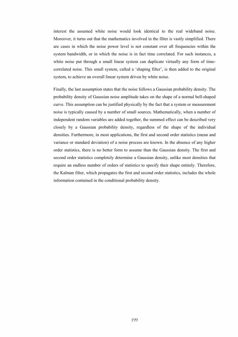
199
interest the assumed white noise would look identical to the real wideband noise.
Moreover, it turns out that the mathematics involved in the filter is vastly simplified. There
are cases in which the noise power level is not constant over all frequencies within the
system bandwidth, or in which the noise is in fact time correlated. For such instances, a
white noise put through a small linear system can duplicate virtually any form of time-
correlated noise. This small system, called a ‘shaping filter’, is then added to the original
system, to achieve an overall linear system driven by white noise.
Finally, the last assumption states that the noise follows a Gaussian probability density. The
probability density of Gaussian noise amplitude takes on the shape of a normal bell-shaped
curve. This assumption can be justified physically by the fact that a system or measurement
noise is typically caused by a number of small sources. Mathematically, when a number of
independent random variables are added together, the summed effect can be described very
closely by a Gaussian probability density, regardless of the shape of the individual
densities. Furthermore, in most applications, the first and second order statistics (mean and
variance or standard deviation) of a noise process are known. In the absence of any higher
order statistics, there is no better form to assume than the Gaussian density. The first and
second order statistics completely determine a Gaussian density, unlike most densities that
require an endless number of orders of statistics to specify their shape entirely. Therefore,
the Kalman filter, which propagates the first and second order statistics, includes the whole
information contained in the conditional probability density.
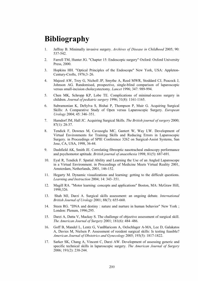
200
Bibliography
1. Jaffray B. Minimally invasive surgery. Archives of Disease in Childhood 2005; 90:
537-542.
2. Farrell TM, Hunter JG. "Chapter 15: Endoscopic surgery" Oxford: Oxford University
Press, 2000.
3. Hopkins HH. "Optical Principles of the Endoscope" New York, USA: Appleton-
Century-Crofts, 1976;3–26.
4. Majeed AW, Troy G, Nicholl JP, Smythe A, Reed MWR, Stoddard CJ, Peacock J,
Johnson AG. Randomised, prospective, single-blind comparison of laparoscopic
versus small-incision cholecystectomy. Lancet 1996; 347: 989-994.
5. Chen MK, Schropp KP, Lobe TE. Complications of minimal-access surgery in
children. Journal of pediatric surgery 1996; 31(8): 1161-1165.
6. Subramonian K, DeSylva S, Bishai P, Thompson P, Muir G. Acquiring Surgical
Skills: A Comparative Study of Open versus Laparoscopic Surgery. European
Urology 2004; 45: 346–351.
7. Hamdorf JM, Hall JC. Acquiring Surgical Skills. The British journal of surgery 2000;
87(1): 28-37.
8. Tendick F, Downes M, Cavusoglu MC, Gantert W, Way LW. Development of
Virtual Environments for Training Skills and Reducing Errors in Laparoscopic
Surgery. in Proceedings of SPIE Conference 3262 on Surgical-Assist Systems, San
Jose, CA, USA, 1998, 36-44.
9. Dashfield AK, Smith JE. Correlating fibreoptic nasotracheal endoscopy performance
and psychomotor aptitude. British journal of anaesthesia 1998; 81(5): 687-691.
10. Eyal R, Tendick F. Spatial Ability and Learning the Use of an Angled Laparoscope
in a Virtual Environment. in Proceedings of Medicine Meets Virtual Reality 2001,
Amsterdam, Netherlands, 2001, 146-152.
11. Hegarty M. Dynamic visualizations and learning: getting to the difficult questions.
Learning and Instruction 2004; 14: 343–351.
12. Magill RA. "Motor learning: concepts and applications" Boston, MA: McGraw Hill,
1998;326.
13. Shah MJ, Darzi A. Surgical skills assessment: an ongoing debate. International
British Journal of Urology 2001; 88(7): 655-660.
14. Steen RG. "DNA and destiny : nature and nurture in human behavior" New York ;
London: Plenum, 1996;295.
15. Darzi A, Datta V, Mackay S. The challenge of objective assessment of surgical skill.
The American Journal of Surgery 2001; 181(6): 484–486.
16. Goff B, Mandel L, Lentz G, VanBlaricom A, Oelschlager A-MA, Lee D, Galakatos
A, Davies M, Nielsen P. Assessment of resident surgical skills: Is testing feasible?
American Journal of Obstetrics and Gynecology 2005; 193(5): 1817-1822.
17. Sarker SK, Chang A, Vincent C, Darzi AW. Development of assessing generic and
specific technical skills in laparoscopic surgery. The American Journal of Surgery
2006; 191(2): 238-244.

201
18. Delp SL, Loan P, Basdogan C, Rosen JM. Surgical Simulation: An Emerging
Technology for Training in Emergency Medicine. Presence 1997; 6(2).
19. Indelicato D. Virtual Reality in Surgical Training. The Dartmouth Undergraduate
Journal of Science 1999; I(1).
20. Gorman PJ, Meier AH, Krummel TM. Simulation and virtual reality in surgical
education: real or unreal? Archieves of Surgery 1999; 134(11): 1203-1208.
21. Liu A, Tendick F, Cleary K, Kaufmann C. A Survey of Surgical Simulation:
Applications, Technology, and Education. Presence 2003; 12(6).
22. Colt HG, Crawford SW, Galbraith O. Virtual Reality Bronchoscopy Simulation: A
Revolution in Procedural Training. Chest 2001; 120: 1333-1339.
23. McCloy R, Stone R. Science, medicine, and the future: Virtual reality In surgery.
British Medical Journal 2001; 323: 912-915.
24. Gallagher AG, Satava RM. Virtual reality as a metric for the assessment of
laparoscopic psychomotor skills. Surgical Endoscopy 2002; 16(12): 1746-1752.
25. Gallagher AG, Smith D, Bowers SP, Seymour NE, Pearson A, McNatt S, Hananel D,
Satava RM. Psychomotor skills assessment in practicing surgeons experienced in
performing advanced laparoscopic procedures. Journal of the American College of
Surgeons 2003; 197(3): 479-488.
26. Hanna GB, Drew T, Clinch P, Hunter B, Cuschieri A. Computer-controlled
endoscopic performance assessment system. Surgical endoscopy 1998; 12(7): 997-
1000.
27. Sokollik C, Gross J, Buess G. New model for skills assessment and training progress
in minimally invasive surgery. Surgical endoscopy 2004; 18(3): 495-500.
28. Nicolaou M, James A, Darzi A, Yang GZ. A study of saccade transition for attention
segregation and task strategy in laparoscopic surgery. in Proceedings of Medical
Image Computing and Computer-Assisted Intervention, Saint-Malo, France, 2004,
97-104.
29. Satava RM. Surgical Education and Surgical Simulation. World Journal of Surgery
2001; 25(11): 1484 - 1489.
30. Bar-Meir S. A New Endoscopic Simulator. Endoscopy 2000; 32: 906-910.
31. Bro-Nielsen M, Tasto JL, Cunningham R, Merril GL. PreOp Endoscopic Simulator:
A PC-Based Immersive Training System. in Proceedings of Medicine Meets Virtual
Reality, San Fransisco, California, USA, 1999, 76–82.
32. Azuma RT. A Survey of Augmented Reality. Presence: Teleoperators and Virtual
Environments 1997; 6(4): 355-385.
33. Haluck RS, Marshall RL, Krummel TM, Melkonian MG. Are surgery training
programs ready for virtual reality? A survey of program directors in general surgery.
Journal of American College of Surgeons 2001; 193(6): 660-665.
34. Stoyanov D, ElHelw M, Lo BP, Chung A, Bello F, Yang G-Z. Current issues of
photorealistic rendering for virtual and augmented reality in minimally invasive
surgery. in Proceedings of Seventh International Conference on Information
Visualization, 2003, London, UK, 2003, 350 - 358.
35. Bro-Nielsen M. Simulation techniques for minimally invasive surgery. Journal of
Minimally Invasive Therapy & Allied Technologies (MITAT) 1997; 6: 106-110.
36. Seymour NE, Rotnes JS. Challenges to the development of complex virtual reality
surgical simulations. Surgical Endoscopy 2006; 20(11): 1774-1777.

202
37. ElHelw MA, Atkins MS, Nicolaou M, Chung AJ, Yang GZ. A Gaze-Based
Framework for Investigating the Perception of Visual Realism in Simulated Scenes.
ACM Transactions on Applied Perception (under review), 2005.
38. Cakmak HK, Kuhnapfel U. Animation and Simulation Techniques for VR-Training
Systems in Endoscopic Surgery. in Proceedings of Eurographics Workshop on
Computer Animation and Simulation, Wien, Austria, 2000, 173-185.
39. Miller K. Biomechanics of soft tissues. Medical science monitor: international
medical journal of experimental and clinical research 2000; 6(1): 158-167.
40. Cootes TF, Taylor CJ, Cooper DH, Graham J. Active shape models: Their training
and application. Computer Vision and Image Understanding 1995; 61(1): 38-59.
41. Zatonyi J, Paget R, Szekely G, Bajka M. Real-time Synthesis of Bleeding for Virtual
Hysteroscopy. Medical image analysis 2005; 9(3): 255-266.
42. Sweet R, Porter J, Oppenheimer P, Hendrickson D, Gupta A, Weghorst S. Simulation
of Bleeding in Endoscopic Procedures Using Virtual Reality. Journal of Endourology
2002; 16(7): 451-455.
43. Stylopoulos N, Cotin S, Dawson S, Ottensmeyer M, Neumann P, Bardsley R, Russell
M, Jackson P, Rattner D. CELTS: A clinically-based Computer Enhanced
Laparoscopic Training System. Stud. Health Technol. Inform. 2003; 94: 336-342.
44. Basdogan C, De S, Kim J, Muniyandi M, Kim H, A.Srinivasan M. Haptics in
minimally invasive surgical simulation and training. IEEE Computer Graphics and
Applications 2004; 24(2): 56-64.
45. Basdogan C, Ho C-H, Srinivasan MA. Virtual environments for medical training:
graphical and haptic simulation of laparoscopic common bile duct exploration.
IEEE/ASME Transactions on Mechatronics (special issue on Haptic Displays and
Applications) 2001; 6(3): 269-285.
46. Weibel ER. Why measure lung structure? Respiratory and Critical Care Medicine
2001; 163(2): 314-315.
47. Sauret V, Halson PM, Brown IW, Fleming JS, Bailey AG. Study of the three-
dimensional geometry of the central conducting airways in man using computed
tomographic (CT) images. The American journal of anatomy 2002; 200(2): 123-134.
48. Jensen OE, "Flows through deformable airways", Deformation: lungs, Date
Accessed: Access,
http://www.biomatematica.it/urbino2002/pages/course_on_line.htm, 2002.
49. Kamm RD. Airway Wall Mechanics. Annual Review of Biomedical Engineering
1999; 1: 47-72.
50. Kaye J, Metaxas D, Clarke JR, Webber B. Lung Modeling: Integrating Anatomy and
Physiology. in Proceedings of First International Symposium on Medical Robotics
and Computer-Assisted Surgery (MRCAS-94), Pittsburgh, USA, 1994.
51. Tooker AC, Hong KS, McKinstry EL, Costello P, Jolesz FA, Albert MS. Distal
Airways in Humans: Dynamic Hyperpolarized (3)He MR Imaging—Feasibility.
Radiology 2003; 227(2): 575-579.
52. Tawil AZ, Thomas G, Lee JD, McLennan G. What's so hard about bronchoscopic
surgery? Identifying the perceptual and cognitive difficulties of bronchoscopic
surgery. in Proceedings of Human Factors and Ergonomics, Houston, Texas, USA,
1999.
53. Buthiau D, Khayat D. "Virtual Endscopy" Berlin: Springer-Verlag, 2003;192.
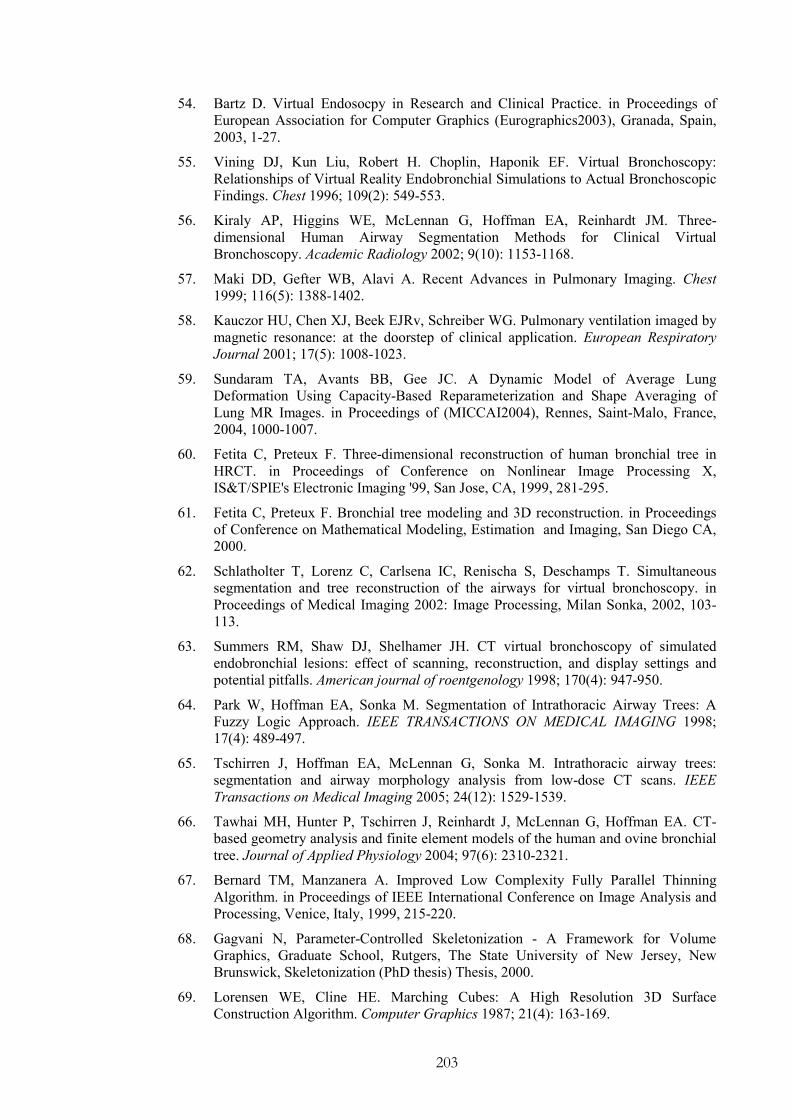
203
54. Bartz D. Virtual Endosocpy in Research and Clinical Practice. in Proceedings of
European Association for Computer Graphics (Eurographics2003), Granada, Spain,
2003, 1-27.
55. Vining DJ, Kun Liu, Robert H. Choplin, Haponik EF. Virtual Bronchoscopy:
Relationships of Virtual Reality Endobronchial Simulations to Actual Bronchoscopic
Findings. Chest 1996; 109(2): 549-553.
56. Kiraly AP, Higgins WE, McLennan G, Hoffman EA, Reinhardt JM. Three-
dimensional Human Airway Segmentation Methods for Clinical Virtual
Bronchoscopy. Academic Radiology 2002; 9(10): 1153-1168.
57. Maki DD, Gefter WB, Alavi A. Recent Advances in Pulmonary Imaging. Chest
1999; 116(5): 1388-1402.
58. Kauczor HU, Chen XJ, Beek EJRv, Schreiber WG. Pulmonary ventilation imaged by
magnetic resonance: at the doorstep of clinical application. European Respiratory
Journal 2001; 17(5): 1008-1023.
59. Sundaram TA, Avants BB, Gee JC. A Dynamic Model of Average Lung
Deformation Using Capacity-Based Reparameterization and Shape Averaging of
Lung MR Images. in Proceedings of (MICCAI2004), Rennes, Saint-Malo, France,
2004, 1000-1007.
60. Fetita C, Preteux F. Three-dimensional reconstruction of human bronchial tree in
HRCT. in Proceedings of Conference on Nonlinear Image Processing X,
IS&T/SPIE's Electronic Imaging '99, San Jose, CA, 1999, 281-295.
61. Fetita C, Preteux F. Bronchial tree modeling and 3D reconstruction. in Proceedings
of Conference on Mathematical Modeling, Estimation and Imaging, San Diego CA,
2000.
62. Schlatholter T, Lorenz C, Carlsena IC, Renischa S, Deschamps T. Simultaneous
segmentation and tree reconstruction of the airways for virtual bronchoscopy. in
Proceedings of Medical Imaging 2002: Image Processing, Milan Sonka, 2002, 103-
113.
63. Summers RM, Shaw DJ, Shelhamer JH. CT virtual bronchoscopy of simulated
endobronchial lesions: effect of scanning, reconstruction, and display settings and
potential pitfalls. American journal of roentgenology 1998; 170(4): 947-950.
64. Park W, Hoffman EA, Sonka M. Segmentation of Intrathoracic Airway Trees: A
Fuzzy Logic Approach. IEEE TRANSACTIONS ON MEDICAL IMAGING 1998;
17(4): 489-497.
65. Tschirren J, Hoffman EA, McLennan G, Sonka M. Intrathoracic airway trees:
segmentation and airway morphology analysis from low-dose CT scans. IEEE
Transactions on Medical Imaging 2005; 24(12): 1529-1539.
66. Tawhai MH, Hunter P, Tschirren J, Reinhardt J, McLennan G, Hoffman EA. CT-
based geometry analysis and finite element models of the human and ovine bronchial
tree. Journal of Applied Physiology 2004; 97(6): 2310-2321.
67. Bernard TM, Manzanera A. Improved Low Complexity Fully Parallel Thinning
Algorithm. in Proceedings of IEEE International Conference on Image Analysis and
Processing, Venice, Italy, 1999, 215-220.
68. Gagvani N, Parameter-Controlled Skeletonization - A Framework for Volume
Graphics, Graduate School, Rutgers, The State University of New Jersey, New
Brunswick, Skeletonization (PhD thesis) Thesis, 2000.
69. Lorensen WE, Cline HE. Marching Cubes: A High Resolution 3D Surface
Construction Algorithm. Computer Graphics 1987; 21(4): 163-169.
204
70. Luebke DP. A Developer’s Survey of Polygonal Simplification Algorithms. IEEE
Computer Graphics and Applications 2001; 21(3): 24-35.
71. ElHelw MA, Chung AJ, Darzi A, Yang GZ. Image-Based Soft Tissue Deformation.
in Proceedings of International Conference on Medical Image Computing and
Computer Assisted Intervention (MICCAI03), 2003, 83-90.
72. Koppel D, Wang Y-F, Lee H. Image-based rendering and modeling in video-
endoscopy. in Proceedings of IEEE International Symposium on Biomedical
Imaging: Macro to Nano, Arlington, VA, USA, 2004, 269-272.
73. Chung AJ, Deligianni F, Shah P, Wells A, Yang GZ. Enhancement of Visual Realism
with BRDF for Patient Specific Bronchoscopy Simulation. in Proceedings of
MICCAI, Rennes, France, 2004.
74. Mori K, Deguchi D, Sugiyama J, Suenaga Y, Toriwaki J-i, Jr. CRM, Takabatake H,
Natori H. Tracking of a bronchoscope using epipolar geometry analysis and
intensity-based image registration of real and virtual endoscopic images. Medical
Image Analysis 2002; 6(3): 181-336.
75. Mori K, Deguchi D, Akiyama K, Kitasaka T, Maurer CR, Suenaga Y, Takabatake H,
Mori M, Natori H. Hybrid Bronchoscope Tracking Using a Magnetic Tracking
Sensor and Image Registration. in Proceedings of International Conference on
Medical Image Computing and Computer Assisted Intervention (MICCAI05), Palm
Springs, California, USA, 2005, 543-550.
76. Helferty JP, Zhang C, McLennan G, Higgins WE. Videoendoscopic distortion
correction and its application to virtual guidance of endoscopy. IEEE Transactions
on Medical Imaging 2001; 20(7): 605-617.
77. Bricault I, Ferretti G, Cinquin P. Registration of real and CT-derived virtual
bronchoscopic images to assist transbronchial biopsy. IEEE Transactions on Medical
Imaging 1998; 17(5): 703-714.
78. Zitova B, Flusser J. Image registration methods: A survey. Image and Vision
Computing 2003; 21(11): 977-1000.
79. Rohr K. Elastic Registration of Multimodal Medical Images: A Survey. KI --
Künstliche Intelligenz 2000; 00(3): 11-17.
80. Maintz JBA, Viergever MA. A survey of medical image registration. Medical Image
Analysis 1998; 2(1): 1-36.
81. Hill DLG, Batchelor PG, Holden M, Hawkes DJ. Medical image registration. Physics
in Medicine and Biology 2001; 46(3): R1-R45.
82. Brown LG. A survey of image registration techniques. ACM Computing Surveys
(CSUR) 1992; 24(4): 325-376.
83. Vilanova A, Konig A, Groller E. VirEn: A Virtual Endoscopy System. Machine
Graphics and Vision 1999; 8(3): 469-487.
84. Nain D, Haker S, Kikinis R, Grimson WEL. An Interactive Virtual Endoscopy Tool.
in Proceedings of Medical Image Computing and Computer-Assisted Intervention
(MICCAI01), Utrecht, The Netherlands, 2001.
85. Lombardo J-C, Cani M-P, Neyret F. Real-time collision detection for virtual surgery.
in Proceedings of IEEE Proceedings in Computer Animation99, Geneva,
Switzerland, 1999, 82-90.
86. Penney GP, Weese J, Little JA, Desmedt P, Hill DL, Hawkes DJ. A Comparison of
Similarity Measures for Use in 2D-3D Medical Image Registration. IEEE
transactions on Medical Imaging 1998; 17(4): 586-595.

205
87. Hajnal J, Hawkes D, Hill D. "Medical Image Registration" CRC Press, 2001.
88. Heikkila J, Silven O. A Four-step Camera Calibration Procedure with Implicit Image
Correction. in Proceedings of IEEE Computer Society Conference on Computer
Vision and Pattern Recognition (CVPR97), San Juan, Puerto Rico, 1997, 1106-1112.
89. Rueckert D, Sonoda Ll, Hayes C, Hill DLG, Leach MO, Hawkes DJ. Nonrigid
registration using free-form deformations: application to breast MR images. IEEE
Transactions on Medical Imaging 1999; 18(8): 712-721.
90. Lee S, Wolberg G, Chwa K-Y, Shin SY. Image metamorphosis with scattered
feature constraints. IEEE Transactions on Visualization and Computer Graphics
1996; 2(4): 337-354.
91. McInerney T, Terzopoulos D. Deformable Models in Medical Image Analysis: A
Survey. Medical Image Analysis 1996; 1(2): 91-108.
92. Meier U, Lopez O, Monserrat C, Juan MC, Alcaniz M. Real-time deformable models
for surgery simulation: a survey. Computer Methods and Programs in Biomedicine
2005; 77(3): 183-197.
93. Wu X, Downes MS, Goktekin T, Tendick F. Adaptive Nonlinear Finite Elements for
Deformable Body Simulation Using Dynamic Progressive Meshes. in Proceedings of
European Association for Computer Graphics (Eurographics), Manchester, UK,
2001, 349-358.
94. Gibson SFF, Mirtich B A survey of deformable models in computer graphics,
Mitsubishi Electric Research Laboratories, Cambridge, MA, USA TR1997-019,
1997.
95. Garrity JM, Segars WP, Knisley SB, Tsui BMW. Development of a dynamic model
for the lung lobes and airway tree in the NCAT phantom. IEEE Transactions on
Nuclear Science 2003; 50(3): 378-383.
96. Holden M, Hill DLG, Denton ERE, Jarosz JM, Cox TCS, Rohlfin T, Goodey J,
Hawkes DJ. Voxel similarity measures for 3-D serial MR brain image registration.
IEEE Transactions on Medical Imaging 2000; 19(2): 94-102.
97. Lo C-H, Don H-S. 3-D moment forms: Their construction and application to object
identification and positioning. IEEE Transactions on Pattern Analysis and Machine
Intelligence 1989; 11(10): 1053-1064.
98. Dinggang S, Davatzikos C. HAMMER: hierarchical attribute matching mechanism
for elastic registration. IEEE Transactions on Medical Imaging 2002; 21(11): 1421-
1439.
99. Viola P, III WMW. Alignment by Maximization of Mutual Information.
International Journal of Computer Vision 1997; 24(2): 137-154.
100. Viola P, Alignment by Maximazation of Mutual Information, Massachusetts Institute
of Technology, Registration: Intensity Based (PhD Thesis) Thesis, 1995.
101. Studholme C, Hill DLG, Hawkes DJ. An Overlap Invariant Entropy Measure of 3D
Medical Image Alignment. Pattern Recognition 1998; 32(1): 71-86.
102. Pluim JPW, Maintz JBA, Viergever MA. Mutual-information-based registration of
medical images: a survey. IEEE Transactions on Medical Imaging 2003; 22(8): 986-
1004.
103. Haber E, Modersitzki J. Intensity gradient based registration and fusion of multi-
modal images. IEEE Transactions of Medical Imaging 2004 (Submitted).

206
104. Thevenaz P, Bierlaire M, Unser M. Halton Sampling for Image Registration Based
on Mutual Information. Sampling Theory in Signal and Image Processing 2006 (In
press).
105. Likar B, Pernus F. A hierarchical approach to elastic registration based on mutual
information. Image and Vision Computing 2001; 19(1-2): 33-44.
106. Clarkson MJ, Rueckert D, Hill DLG, Hawkes DJ. Using Photo-Consistency to
Register 2D Optical Images of the Human Face to a 3D Surface Model. IEEE
Transactions of Pattern analysis and Machine Intelligence 2001; 23(11): 1266-1280.
107. Pennec X, Ayache N, Thirion J-P. "Landmark-based registration using features
identified through differential geometry" San Diego: Academic Press, 2000;499-513.
108. Chui H, Rangarajan A. A new point matching algorithm for non-rigid registration.
Computer Vision and Image Understanding 2003; 89(2-3): 114-141.
109. Gold S, Rangarajan A, Lu CP, Pappu S, Mjolsness E. New Algorithms for 2D and
3D Point Matching: Pose Estimation and Correspondence. Pattern Recognition 1998;
31(8): 1019-1031.
110. DeMenthon D, David P, Samet H SoftPOSIT: An Algorithm for Registration of 3D
Models to Noisy Perspective Images Combining Softassign and POSIT, Center for
Automation Research, Computer Science Department, UCLA CAR-TR-969, CS-TR-
4257, 2001.
111. David P, DeMenthon D, Duraiswami R, Samet H. SoftPOSIT: Simultaneous Pose
and Correspondence Determination. in Proceedings of European Conference on
Computer Vision 2002 (ECCV'02), Copenhagen, 2002.
112. Kraats EBvd, Penney GP, Tomazevic D, Walsum Tv, Niessen WJ. Standardized
Evaluation of 2D-3D Registration. in Proceedings of Medical Image Computing and
Computer-Assisted Intervention (MICCAI04), Saint-Malo, France, 2004, 574-581.
113. Helferty JP, Higgins WE. Technique for Registering 3D Virtual CT Images to
Endoscopic Video. in Proceedings of 2001 IEEE International Conference on Image
Processing (ICIP'01), Thessaloniki, Greece, 2001, 893-896.
114. Helferty JP, Higgins WE. Combined Endoscopic Video Tracking and Virtual 3D CT
Registration for Surgical Guidance. in Proceedings of International Conference on
Image Processing, IEEE 2002 (ICIP'00), Rochester, New York, 2002.
115. Rashid HU, Burger P. Differential algorithm for the determination of shape from
shading using a point light source. Image and Vision Computing 1992; 10(2): 119-
127.
116. Horn BKP, Berthold KP. "Shape from Shading" B. K. Horn, M. J. Brooks ed.,
Cambridge: MIT Press, 1989.
117. Horn BKP. Understanding Image Intensities. Artificial Intelligence 1977; 8(2): 201-
231.
118. Horn BKP. "Robot Vision" Cambridge: MIT Press, 1986.
119. Ramachandran VS. Perception of Shape from Shading. Nature 1988; 331(6152): 163-
166.
120. Kleffner DA, Ramachandran VS. On the perception of shape from shading.
Perception and Psychophysics 1992; 52(1): 18-36.
121. Oliensis J. Uniqueness in Shape from Shading. International Journal of Computer
Vision 1991; 6(2): 75-104.
207
122. Forsyth D, Zisserman A. Reflections on Shading. IEEE Transactions on Pattern
Analysis and Machine Intelligence 1991; 13(7): 671-679.
123. Nayar SK, Ikeuchi K, Kanade T. Surface Reflection: Physical and Geometrical
Perspectives. IEEE Transactions on Pattern Analysis and Machine Intelligence 1991;
13(7): 611-634.
124. Kimmel R, Bruckstein AM. Global Shape from Shading. Computer Vision and Image
Understanding 1995; 62(3): 360-369.
125. Rashid H, Shape from Shading and motion parameter estimation under near point
light source illumination, Imperial College of Science, Technology and Medicine,
London, Shape from Shading (PhD Thesis) Thesis, 1991.
126. Bichsel M, Pentland AP. A simple algorithm for shape from shading. in Proceedings
of IEEE Computer Society Conference on Computer Vision and Pattern Recognition
(CVPR '92), Champaign, IL USA, 1992, 459 - 465.
127. Oliensis J. Shape from shading as a partially well-constrained problem. Computer
Vision, Graphics, and Image Processing: Image Understanding 1991; 54(2): 163-
183.
128. Tsai P-S, Shah M. A fast linear shape from shading. in Proceedings of IEEE
Computer Society Conference on Computer Vision and Pattern Recognition (CVPR
'92), Champaign, IL USA, 1992, 734 - 736.
129. Worthington PL, Hancock ER. New constraints on data-closeness and needle map
consistency for shape-from-shading. IEEE Transactions on Pattern Analysis and
Machine Intelligence 1999; 21(12): 1250-1267.
130. Okatani T, Deguchi K. Shape Reconstruction from an Endoscope Image by shape
from shading technique for a point light source at the projection centre. Computer
Vision and Image Understanding 1997; 66(2): 119-131.
131. Forster CHQ, Tozzi CL. Towards 3D Reconstruction of Endoscope Images using
Shape from Shading. in Proceedings of XIII Brizilian Symposium on Computer
Graphics and Image Processing (SIBGRAPI'00), Gramado, Brazil, 2000, 90-96.
132. Prados E, Application of the theory of the viscosity solutions to the shape from
shading problem, NICE, Sophia Antipolis, France, 2004.
133. Deguchi K, Okatani T. Shape reconstruction from an endoscope image by shape-
from-shading technique for a point light source at the projection center. in
Proceedings of IEEE Workshop on Mathematical Methods in Biomedical Image
Analysis, San Francisco, CA, USA, 1996, 290-298.
134. Agrawal A, Chellappa R, Raskar R. An Algebraic Approach to Surface
Reconstruction from Gradient Fields. in Proceedings of IEEE International
Conference on Computer Vision, 2005.
135. Zhang C, Helferty JP, McLennan G, Higgins WE. Nonlinear distortion correction in
endoscopic video images. in Proceedings of International Conference on Image
Processing, 2000, Vancouver, BC Canada, 2000, 439 - 442.
136. Yang GZ, Burger P, Firmin DN, Underwood SR. Structure adaptive anisotropic
image filtering. Image and Vision Computing 1994; 14(2): 135-145.
137. Naga J, Mori K, Enjouji T, Deguchi D, Kitasaka T, Suenaga Y, Hasegawa J-i,
Toriwak J-i, Takabatake H, Natori H. Fast and Accurate Bronchoscope Tracking
Using Image Registration and Motion Prediction. in Proceedings of Medical Image
Computing and Computer-Assisted Intervention (MICCAI04), Saint-Malo, France,
2004, 551-558.

208
138. Maybeck PS. "Stochastic models, estimation and control - Chapter1: Introduction"
Ohio: Academic Press, 1979.
139. Blake A, Isard M. "Active Contours" London: Springer, 1998.
140. Wildenberg AP, Learning and Initialisation for Visual Tracking, University of
Oxford, Oxford, UK, Modular Training for Visual Tracking Thesis, 1998.
141. North B, Blake A, Isard M, Rittscher J. Learning and classification of complex
dynamics. IEEE Transactions on Pattern Analysis and Machine Intelligence 2000;
22(9): 1016-1034.
142. Zhou Y A Kalman Filter Based Registration Approach for Multiple Asynchronous
Sensors, Defence Research and Development Canada, Ottawa Canada 2003.
143. Isard M, Blake A. CONDENSATION-Conditional Density Propagation for Visual
Tracking. International Journal of Computer Vision 1998; 29(1): 5-28.
144. Blake A, Isard M, Reynard D. Learning to track the visual motion of contours.
Artificial Intelligence 1995; 78(1-2): 179-212.
145. Arulampalam MS, Maskell S, Gordon N, Clapp T. A tutorial on particle filters for
online nonlinear/non-Gaussian Bayesian tracking. IEEE Transactions on Signal
Processing 2002; 50(2): 174-188.
146. Isard M, Blake A. Contour Tracking By Stochastic Propagation of Conditional
Density. in Proceedings of European Conference on Computer Vision (ECCV96),
Cambridge, UK, 1996, 343-356.
147. Davison AJ. Simultaneous localization and map-building using active vision. IEEE
Transactions on Pattern Analysis and Machine Intelligence 2002; 24(7): 865 - 880.
148. Reynard D, Wildenberg A, Blake A, Marchant J. Learning Dynamics of Complex
Motion from Image Sequences. in Proceedings of European Conference in Computer
Vision (ECCV96), Cambridge, UK, 1996, 357-368.
149. Peters TM. Image-guided surgery: from X-rays to virtual reality. Computer Methods
in Biomechanics and Biomedical Engineering 2000; 4(1): 27-57.
150. Cleary K, Clifford M, Stoianovici D, Freedman M, Mun SK, Watson V. Technology
improvements for image-guided and minimally invasive spine procedures. IEEE
Transactions on Information Technology in Biomedicine 2002; 6(4): 249-261.
151. Birkfellner W, Watzinger F, Wanschitz F, Ewers R, Bergmann H. Calibration of
tracking systems in a surgical environment. IEEE Transactions on Medical Imaging
1998; 17(5): 737 - 742.
152. Ecke U, Luebben B, Maurer J, Boor S, Mann WJ. Comparison of Different
Computer-Aided Surgery Systems in Skull Base Surgery. Skull Base 2003; 13(1): 43-
50.
153. Nielsen JC, Kottkamp H, Piorkowski C, Gerds-Li J-H, Tanner H, Hindricks G.
Radiofrequency ablation in children and adolescents: results in 154 consecutive
patients. Europace 2006; 8(5): 323-329.
154. Solomon SB, White PJ, Wiener CM, Orens JB, Wang KP. Three-dimensional CT-
Guided Bronchoscopy With a Real-Time Electromagnetic Position Sensor: A
Comparison of Two Image Registration Methods. Chest 2000; 118(6): 1783-1787.
155. Ellsmere J, Stoll J, WilliamWells, Kikinis R, Vosburgh K, Kane R, Brooks D,
Rattner D. A new visualization technique for laparoscopic ultrasonography. Surgery
2004; 136(1): 84-92.

209
156. Zaaroor M, Bejerano Y, Weinfeld Z, Ben-Haim S. Novel Magnetic Technology for
Intraoperative Intracranial Frameless Navigation: In Vivo and in Vitro Results.
Neurosurgery 2001; 48(5): 1100-1107.
157. Dickfeld T, Calkins H, Zviman M, Meininger G, Lickfett L, Roguin A, Lardo AC,
Berger R, Halperin H, Solomon SB. Stereotactic Magnetic Resonance Guidance for
Anatomically Targeted Ablations of the Fossa Ovalis and the Left Atrium. Journal of
Interventional Cardiac Electrophysiology 2004; 11(2): 105-115.
158. Hummel J, Figl M, Kollmann C, Bergmann H. Evaluation of a miniature
electromagnetic position tracker. Medical physics 2002; 29(10): 2205-2212.
159. Frantz DD, Wiles AD, Leis SE, Kirsch SR. Accuracy assessment protocols for
electromagnetic tracking systems. Phyisics in Medicine and Biology 2003; 48: 2241-
2251.
160. Chung AJ, Edwards PJ, Deligianni F, Yang GZ. Freehand Cocalibration of an
Optical and Electromagnetic Tracker for Navigated Bronchoscopy. in Proceedings of
The Second International Workshop on Medical Imaging and Augmented Reality
(MIAR 2004), Beijing, China, 2004.
161. Schicho K, Figl M, Donat M, Birkfellner W, Seemann R, Wagner A, Bergmann H,
Ewers R. Stability of miniature electromagnetic tracking systems. Physics in
Medicine and Biology 2005; 50(9): 2089-2098.
162. Krueger S, Timinger H, Grewer R, Borgert J. Modality-integrated magnetic catheter
tracking for x-ray vascular interventions. Phyisics in Medicine and Biology 2005;
50(4): 581-597.
163. Wilson E, Slack R, Banovac F, Dieterich S, Zhanga H, Clearya K. Electromagnetic
tracker accuracy in the CyberKnife suite. in Proceedings of Medical Imaging 2006:
Visualization, Image-Guided Procedures, and Display (SPIE), 2006.
164. Cleary K, Banovac F, Levy E, Tanaka D. Development of a Liver Respiratory
Motion Simulator to Investigate Magnetic Tracking for Abdominal Interventions. in
Proceedings of SPIE Medical Imaging 2002 (Visualization, Image-Guided
Procedures, and Display), San Diego, California USA, 2002, 25-29.
165. Banovac F, Glossop N, Lindisch D, Tanaka D, Levy E, Cleary K. Liver tumor biopsy
in a respiring phantom with the assistance of a novel electromagnetic navigation
device. in Proceedings of Conference on Medical Image Computing and Computer
Assisted Intervention (MICCAI02), Tokyo, Japan, 2002, 200-207.
166. Timinger H, Krueger S, Borgert J, Grewer R. Motion compensation for interventional
navigation on 3D static roadmaps based on an affine model and gating. Phyisics in
Medicine and Biology 2004; 49(5): 719-732.
167. Wu X, Taylor R. A Direction Space Interpolation Technique for Calibration of
Electromagnetic Surgical Navigation Systems. in Proceedings of Medical Image
Computing and Computer-Assisted Intervention (MICCAI03), Montréal, Canada,
2003, 215 - 222.
168. Kindratenko VV. A survey of electromagnetic position tracker calibration techniques.
Virtual Reality: Research, Development and Applications 2000; 5(3): 169-182.
169. Horn BKP. Closed-form solution of absolute orientation using unit quaternions.
Optical Society of America A 1987; 4(4): 629-642.
170. Horn BKP, Hilden HM, Negahdaripour S. Closed-form solution of absolute
orientation using orthonormal matrices. Journal of the Optical Society of America A
(JOSA A: Optics, Image Science, and Vision) 1988; 5(7): 1127-1135.

210
171. Barry CD, Allott CP, John NW, Mellor PM, Arundel PA, Thomson DS, Waterton JC.
Three-Dimensional Freehand Ultrasound: Image Reconstruction and Volume
Analysis. Ultrasound in medicine and biology 1997; 23(8): 1209-1224.
172. Borgert J, Kruger S, Timinger H, Krucker J, Glossop N, Durrani A, Viswanathan A,
Wood BJ. Respiratory Motion Compensation with Tracked Internal and External
Sensors during CT Guided Procedures. Computer Aided Surgery 2006; 11(3): 119-
125.
173. Nikolopoulos S, Alexandridi A, Nikolakeas S, Manis G. Experimental analysis of
heart rate variability of long-recording electrocardiograms in normal subjects and
patients with coronary artery disease and normal left ventricular function. Journal of
Biomedical Informatics 2003; 36(3): 202-217.
174. Promayon E, Baconnier P, Puech C. Physically-Based Model for Simulating the
Human Trunk Respiratorion Movements. in Proceedings of Virtual Reality and
Robotics in Medicine and Medial Robotics and Computer-Assisted Surgery
(CVRMed-MRCAS 1997), Grenoble, France, 1997, 379-388.
175. Kaye J, Jr. FPP, Metaxas D. Anatomical and Physiological Simulation for
Respiratory Mechanics. Journal of Image Guided Surgery 1998; 1(3): 164-171.
176. Ruprecht D, Muller H. Image warping with scattered data interpolation. IEEE
Computer Graphics and Applications 1995; 15(2): 37-43.
177. Nelder JA, Mead R. A simplex method for function minimization. Computer Journal
1965; 7: 308-315.
178. Cebral JR, Summers RM. Tracheal and central bronchial aerodynamics using virtual
bronchoscopy and computational fluid dynamics. IEEE Transactions on Medical
Imaging 2004; 23(8): 1021-1033.
179. Horkaew P, Merrifield R, Yang GZ. Building Optimal Statistical Deformable Surface
Models. in Proceedings of International IEEE EMBS Special Topic Conference on
Information Technology Applications in Biomedicine, Birmingham, UK, 2003, 215-
218.
180. Ragheb H, Hancock ER. A probabilistic frameworkfor specular shape-from-shading.
Pattern Recognition 2003; 36(2): 407-427.
181. Welch G, Bishop G. An Introduction to the Kalman Filter. in Proceedings of ACM
SIGGRAPH, 2001.
182. Goodwin GC, Sin KS. "Adaptive filtering prediction and control" New Jersey:
Prentice-Hall, 1984.
183. Fujimoto O, Okita Y, Ozaki S. Nonlinearity-Compensation Extended Kalman Filter
and Its Application to Target Motion Analysis. Oki Technical Review 1997; 63(159).