Embed Size (px)
Citation preview

Vision Techniques and Autonomous Navigation for
an Unmanned Mobile Robot
A thesis submitted to the
Division of Graduate Studies and Research
of the University of Cincinnati
in partial fulfillment of the
requirements for the degree of
MASTER OF SCIENCE
In the Department of Mechanical, Industrial and Nuclear Engineering
Of the College of Engineering
1999
by
Jin Cao
B.S., ( Mechanical Engineering), Tianjin University, China, 1995
Thesis Advisor and Committee Chair: Dr. Ernest L. Hall

2
Dedicated To My Mother

3
Contents
Abstract
Acknowledgements
List of figures …………………………………………………………6
1. Introduction …………………………………………………………8
1.1 Autonomous Vehicles …………………………………………8
1.2. Context …………………………………………………………10
1.3. The Performance Specification of the Research …………………11
1.4. Objective and Contribution of this Work …………………………12
1.5. Outline of the Thesis ………………………………………12
2. Literature Review …………………………………………………14
3. Navigation Technology for Autonomous Guided Vehicles …………………19
3.1. System and Methods for Mobile Robot Navigation …………………20
3.2. Reactive Navigation …………………………………………22
4. An Introduction to Robot Vision Algorithms and Techniques …………24
4.1. Introduction …………………………………………24
4.2. Robot Vision Hardware Component …………………………25
4.3. Image Functions and Characteristics …………………………26
4.4. Image Processing Techniques …………………………32
4.5. Image Recognition and Decisions …………………………48
4.6. Future Development of Robot Vision …………………………55
5. Mobile Robot System Design and Vision-based Navigation System ………57

4
5.1. Introduction …………………………………………………57
5.2. System Design and Development …………………………………58
5.3. Robot’s Kinematics Analysis …………………………………62
5.4. Vision Guidance System and Stereo Vision …………………………63
6. A Neuro-fuzzy Method for Reactive Navigation …………………69
6.1. Neuro-fuzzy Technology …………………………………………69
6.2. Fuzzy Set Definition for the Navigation System …………………70
6.3. Input Membership …………………………………………71
6.4. A Neuro-fuzzy Hybrid System …………………………………72
6.5. The Neuro-fuzzy Architecture …………………………………72
6.6. The Implementation of Fuzzy Rules …………………………………73
6.7. Training and Simulation …………………………………74
7. Conclusions …………………………………………………………76
References …………………………………………………………77
Appendix …………………………………………………………84

5
Abstract
Robot navigation is defined as the technique for guiding a mobile robot to a desired
destination or along a desired path in an environment characterized by a variable terrain
and a set of distinct objects, such as obstacles and landmarks. The autonomous navigation
ability and road following precision are mainly influenced by the control strategy and
real-time control performance. Neural networks and fuzzy logic control techniques can
improve real-time control performance for a mobile robot due to their high robustness
and error-tolerance ability. For a mobile robot to navigate automatically and rapidly, an
important factor is to identify and classify mobile robots’ currently perceptual
environment.
In this thesis, a new approach to the current perceptual environment feature identification
and classification problem, which is based on the analysis of the classifying neural
network and the Neuro-fuzzy algorithm, is presented. The significance of this work lies
in the development of a new method for mobile robot navigation.
6
List of figures
Figure 1. The Bearcat II Mobile Robot
Figure 2. Image at Various Spatial Resolutions
Figure 3. A Digitized Image
Figure 4. Color Cube Shows the Three Dimensional Nature of Color
Figure 5. A Square on a Light Background
Figure 6. Histogram with Bi-model Distribution Containing Two Peaks
Figure 7. Original Image Before Histogram Equalization
Figure 8. New Image After Histogram Equalization
Figure 9. Image Thresholding
Figure 10. A Digitized Image From a Camera
Figure 11. The Original Image Corrupted with Noise
Figure 12. The Noisy Image Filtered by a Gaussian of Variance 3
Figure 13. The Vertical Edges of the Original Image
Figure 14. The Horizontal Edges of the Original Image
Figure 15. The Magnitude of the Gradient
Figure 16. Thresholding of the Peaks of the Magnitude of the Gradient
Figure 17. Edges of the Original Image
Figure 18. A Schematic Diagram of a Single Biological Neuron.
Figure 19. ANN Model Proposed by McCulloch and Pitts in 1943.
Figure 20. Feed-forward Neural Network
Figure 21. The System Block Diagram

7
Figure 22. The Mobile Robot’s Motion
Figure 23. Camera Image Model
Figure 24. The Model of the Mobile Robot in the Obstacle Course
Figure 25. Fuzzy Logic Input Membership
Figure 26. The Schematic of a Neuro-fuzzy System Architecture
Figure 27. Neuro-fuzzy Architecture
8
Chapter 1.
INTRODUCTION
1.1. Autonomous Vehicles
Automatically guided vehicles are becoming increasingly significant in industrial,
commercial and scientific applications. Various kinds of mobile robots are being
introduced into many application situations, such as automatic exploration of dangerous
regions, automatic transfer of articles, and so on. The development of practical and useful
unmanned autonomous vehicles continues to present a challenge to researchers and
system developers.
Two divergent research areas have emerged in the mobile robotics community. In
autonomous vehicle robot research, the goal is to develop a vehicle that can navigate at
relatively high speeds using sensory feedback in outdoor environments such as fields or
roads. These vehicles require massive computational power and powerful sensors in order
to adapt their perception and control capabilities to the high speed of motion in
complicated outdoor environments. The second area of the research deals with mobile
robots that are designed to work in indoor environments or in relatively controlled
outdoor environments. [1]
9
The problem of autonomous navigation of mobile vehicles, or Automated Guided
Vehicles (AGV), involves certain complexities that are not usually encountered in other
robotic research areas. In order to achieve autonomous navigation, the real-time decision
making must be based on continuous sensor information from their environment, either in
indoor or outdoor environments, rather than off-line planning.
An intelligent machine such as mobile robot that must adapt to the changes of its
environment must also be equipped with a vision system so that it can collect visual
information and use this information to adapt to its environment. Under a “general” and
adaptable control structure, a mobile robot is able to make decisions on its navigation
tactics, modify its relative position, navigate itself way around safely or follow the known
path.
Autonomous navigation requires a number of heterogeneous capabilities, including the
ability to execute elementary goal-achieving actions, like reaching a given location; to
react in real time to unexpected events, like the sudden appearance of an obstacle; to
build, use and maintain a map of the environment; to determine the robot's position with
respect to this map; to form plans that pursue specific goals or avoid undesired situations;
and to adapt to changes in the environment.
1.2. Context

10
The autonomous mobile robot, the Bearcat II as shown in Figure 1, which has been used
in this research, was designed by the UC robot Team for the 1999 International Ground
Robotics Competition (IGRC) sponsored by the Autonomous Unmanned Vehicle Society
(AUVS), the U.S. Army TACOM, United Defense, the Society of Automotive Engineers,
Fanuc Robotics and others.
Figure 1. The Bearcat II mobile robot
The robot base is constructed from an 80/20 aluminum Industrial Erector Set. The AGV
is driven and steered by two independent 24 volt, 12 amp motors. These motors drive the
left and right drive wheel respectively through two independent gearboxes, which
increase the motor torque by about forty times. The power to each individual motor is
delivered from a BDC 12 amplifier that amplifies the signal from the Galil DMC motion
controller. To complete the control loops a position encoder is attached on the shaft of
each of the drive motors. The encoder position signal is numerically differentiated to
11
provide velocity feedback signal. There is a castor wheel in the rear of the vehicle, which
is free to swing when the vehicle has to negotiate a turn.
The design objective was to obtain a stable control over the motion with good phase and
gain margins and a fast unit step response. For this purpose a Galil motion control board
was used that has the proportional integral derivative controller (PID) digital control to
provide the necessary compensation required in the control of the motor. The system was
modeled in MATLAB using SIMULINK and the three parameters of the PID controller
were selected using a simulation model to obtain the optimum response. Also, all the
subsystem level components have been chosen to be modular in design and independent
in terms of configuration so as to increase adaptability and flexibility. This enables
replacing of existing components with more sophisticated or suitable ones, as they
become available.
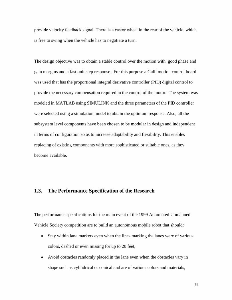
1.3. The Performance Specification of the Research
The performance specifications for the main event of the 1999 Automated Unmanned
Vehicle Society competition are to build an autonomous mobile robot that should:
� Stay within lane markers even when the lines marking the lanes were of various
colors, dashed or even missing for up to 20 feet,
� Avoid obstacles randomly placed in the lane even when the obstacles vary in
shape such as cylindrical or conical and are of various colors and materials,

12
� Adapt to variations in terrain surfaces such as grass, sand, board and asphalt or to
elevation variations.
� Navigate avoiding minor obstacles on the road – for the road hazard event.
� Follow a leader vehicle, which has a specially marked target plate.
1.4. Objective and Contribution of this Work
The objective of this research was to develop a vision-based neuro-fuzzy control method
for navigation of an Autonomous Guided Vehicle (AGV) robot. The autonomous
navigation ability and road following precision are mainly influenced by its control
strategy and real-time control performance. Neural networks and fuzzy logic control
techniques can improve real-time control performance for a mobile robot due to its high
robustness and error-tolerance ability. For a mobile robot to navigate automatically and
rapidly, an important factor is to identify and classify mobile robots’ currently perceptual
environment. The significance of this work lies in the development of a new method for
vision-based mobile robot navigation.
1.5. Outline of the Thesis

13
This research work is organized into seven chapters. Chapter 1 presents a discussion on
the problem statement and research background, as well as the need for the proposed
research and the performance specifications of the system. Chapter 2 discusses existing
literature in this field. Chapter 3 deals with the technologies of autonomous navigation
for the mobile robot. Chapter 4 presents an introduction to the robot vision algorithms
and techniques. Chapter 5 deals with the description of the Bearcat II robot, the structural
design, system design and development, and the vision guidance algorithm and system.
Chapter 6 proposes a novel navigation method for the mobile robot by using neuro-fuzzy
technology. Chapter 7 concludes the thesis with some recommendations and areas of
improvement that for the future.
14
Chapter 2.
LITERATURE REVIEW
In the past, sensor based navigation systems typically relied on ultrasonic sensors or laser
scanners providing one dimensional distance profiles. The major advantage of this type
of sensor results from their ability to directly provide the distance information needed for
collision avoidance. In addition, various methods for constructing maps and environment
models needed for long term as well as for short term (reactive) planning have been
developed.
Due to the large amount of work currently being done in this field it is not possible to
completely discuss all related work. Wichert [2] divided the research work into three
different groups of systems that can be identified in the literature.
� A large number of systems navigate with conventional distance sensors and
use vision to find and identify objects to be manipulated.
� There are several systems that directly couple the sensor output to motor
control in a supervised learning process. The goal is to learn basic skills like
road following or docking. Typically non-complex scenes are presented to
these systems, allowing simplifying assumptions concerning the image
processing itself.
� Vision sensors produce a huge amount of data that have to be examined. To
reduce the massive data flow, most systems really navigating using cameras,

15
predefine relevant low level (e.g. edges, planes) and high level (e.g. objects,
doors, etc.) features to be included in the environment model. These basic
features have to be chosen and modeled in advance. In addition a sensor
processing system has to be established to guarantee proper identification of
the modeled features in the sensor data. Some of the systems aim at
constructing models for unknown environments once the landmarks have been
modeled.
Michaud, et al. [3] present an approach that allows a robot to learn a model of its
interactions with its operating environment in order to manage them according to the
experienced dynamics. Most of existing robots learning methods have considered the
environment where their robots work, unchanged, therefore, the robots have to learn from
scratch if they encounter new environments. Minato, et al. [4] proposes a method which
adapts robots to environmental changes by efficiently transferring a learned policy in the
previous environments into a new one and effectively modifying it to cope with these
changes.
Fuzzy logic has been widely used in the navigation algorithm. Mora, et al. [5] presented a
fuzzy logic-based real-time navigation controller for a mobile robot. The robot makes
intelligent decisions based only on current sensory input as it navigates through the
world. Kim, et al. [6] utilizes fuzzy multi-attribute decision-making method in deciding
which via-point the robot would proceed at each decision step. Via-point is defined as the
local target point of the robot’s movement at each decision instance. At each decision
16
step, a set of the candidates for the next via-point in 2D-navigation space is constructed
by combining various heading angles and velocities. Watanabe, et al. [7] applied a fuzzy
model approach to the control of a time-varying rotational angle, in which multiple linear
models are obtained by utilizing the original nonlinear model in some representative
angles and they are used to derive the optimal type 2 servo gain matrices. Chio, et al. [8]
also presented some new navigation strategy for an intelligent mobile robot.
The applications of Artificial Neural Network (ANN) focus on recognition and
classification of path features during navigation of mobile robot. Vercelli and Morasso
[9] described a method that is an incremental learning and classification technique based
on a self-organizing neural model. Two different self-organizing networks are used to
encode occupancy bitmaps generated from sonar patterns in terms of obstacle boundaries
and free paths, and heuristic procedures are applied to these growing networks to add and
prune units, to determine topological correctness between units, to distinguish and
categorize features. Neural networks have been widely used for the mobile robot
navigation. Streilein, et al. [10] described a novel approach to sonar-based object
recognition for use on an autonomous robot. Dracopoulos and Dimitris [11] presents the
application of multilayer perceptrons to the robot path planning problem and in particular
to the task of maze navigation. Zhu and Yang [12] present recent results of integrating
omni-directional view image analysis and a set of adaptive back propagation networks to
understand the outdoor road scene by a mobile robot.

17
The modern electro-mechanical engineering technician/technologist must function in an
increasingly automated world of design and manufacturing of today’s products
[13][14][15][16]. To navigate and recognize where it is, a mobile robot must be able to
identify its current location. The more the robot knows about its environment, the more
efficiently it can operate. Grudic,et al. [17] used a nonparametric learning algorithm to
build a robust mapping between an image obtained from a mobile robot’s on-board
camera, and the robot’s current position. It used the learning data obtained from these raw
pixel values to automatically choose a structure for the mapping without human
intervention, or any a priori assumptions about what type of image features should be
used.
In order to localize itself, a mobile robot tries to match its sensory information at any
instant against a prior environment model, the map [18]. A probabilistic map can be
regarded as a model that stores at each robot configuration the probability density
function of the sensor readings at the robot configuration. Vlassis, et al. [19] described a
novel sensor model and a method for maintaining a probabilistic map in cases of dynamic
environments.
Some new methods are proposed based on recent web technologies such as browsers,
Java language and socket communication. It allows users to connect to robots through a
web server, using their hand-held computers, and to monitor and control the robots via
various input devices. Hiraishi, et al. [20] described a web-based method for

18
communication with and control of heterogeneous robots in a unified manner, including
mobile robots and vision sensors.
A Neural integrated fuzzy controller (NiF-T) which integrates the fuzzy logic
representation of human knowledge with the learning capability of neural networks has
been developed for nonlinear dynamic control problems. Ng, et al [21] developed a
neural integrated Fuzzy conTroller (NiF-T) which integrates the fuzzy logic
representation of human knowledge with the learning capability of neural networks.
Daxwanger, et al. [22] presented their neuro-fuzzy approach to visual guidance of a
mobile robot vehicle.
Robotics in the near future will incorporate machine learning, human-robot interaction,
multi-agent behavior, humanoid robots, and emotional components. Most of these
features also characterize developments in software agents. In general, it is expected that
in the future the boundary between softbots and robots may become increasingly fuzzy,
as the software and hardware agents being developed become more intelligent, have
greater ability to learn from experience, and to interact with each other and with humans
in new and unexpected ways. [23]

19
Chapter 3.
NAVIGATION TECHNOLOGY FOR
AUTONOMOUS GUIDED VEHILCES
A navigation system is the method for guiding a vehicle. Since the vehicle is in
continuous motion, the navigation system should extract a representation of the world
from the moving images that it receives. The last fifteen years have seen a very large
amount of literature on the interpretation of motion fields as regards the information they
contain about the 3-D world. In general, the problem is compounded by the fact that the
information that can be derived from the sequence of images is not the exact projection of
the 3D-motion field, but rather only information about the movement of light patterns,
optical flow.
About 40 years ago, Hubel and Wiesel [24] studied the visual cortex of the cat and found
simple, complex, and hypercomplex cells. In fact, vision in animals is connected with
action in two senses: “vision for action” and “action for vision”. [25]
The general theory for mobile robotics navigation is based on a simple premise. For a
mobile robot to operate it must sense the known world, be able to plan its operations and
then act based on this model. This theory of operation has become known as SMPA
(Sense, Map, Plan, and Act).

20
SMPA was accepted as the normal theory until around 1984 when a number of people
started to think about the more general problem of organizing intelligence. There was a
requirement that intelligence be reactive to dynamic aspects of the unknown
environments, that a mobile robot operate on time scales similar to those of animals and
humans, and that intelligence be able to generate robust behavior in the face of uncertain
sensors, unpredictable environments, an a changing world. This led to the development of
the theory of reactive navigation by using Artificial Intelligence (AI). [26]
3.1. Systems and Methods for mobile robot navigation
Odometry and Other Dead-Reckoning Methods
Odometry is one of the most widely used navigation methods for mobile robot
positioning. It provides good short-term accuracy, an inexpensive facility, and allows
high sampling rates. [27]
This method uses encoders to measure wheel rotation and/or steering orientation.
Odometry has the advantage that it is totally self-contained, and it is always capable of
providing the vehicle with an estimate of its position. The disadvantage of odometry is
that the position error grows without bound unless an independent reference is used
periodically to reduce the error.
21
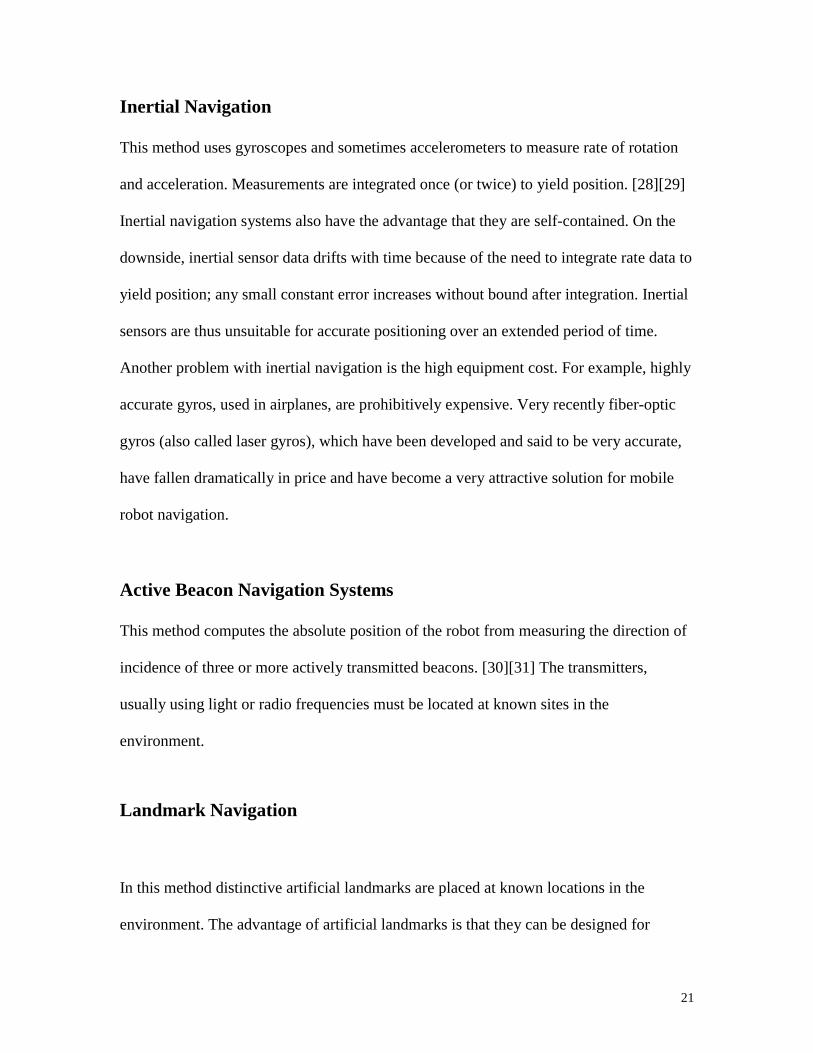
Inertial Navigation
This method uses gyroscopes and sometimes accelerometers to measure rate of rotation
and acceleration. Measurements are integrated once (or twice) to yield position. [28][29]
Inertial navigation systems also have the advantage that they are self-contained. On the
downside, inertial sensor data drifts with time because of the need to integrate rate data to
yield position; any small constant error increases without bound after integration. Inertial
sensors are thus unsuitable for accurate positioning over an extended period of time.
Another problem with inertial navigation is the high equipment cost. For example, highly
accurate gyros, used in airplanes, are prohibitively expensive. Very recently fiber-optic
gyros (also called laser gyros), which have been developed and said to be very accurate,
have fallen dramatically in price and have become a very attractive solution for mobile
robot navigation.
Active Beacon Navigation Systems
This method computes the absolute position of the robot from measuring the direction of
incidence of three or more actively transmitted beacons. [30][31] The transmitters,
usually using light or radio frequencies must be located at known sites in the
environment.
Landmark Navigation
In this method distinctive artificial landmarks are placed at known locations in the
environment. The advantage of artificial landmarks is that they can be designed for

22
optimal detectability even under adverse environmental conditions. [32][33] As with
active beacons, three or more landmarks must be "in view" to allow position estimation.
Landmark positioning has the advantage that the position errors are bounded, but
detection of external landmarks and real-time position fixing may not always be possible.
Unlike the usually point-shaped beacons, artificial landmarks may be defined as a set of
features, e.g., a shape or an area. Additional information, for example distance, can be
derived from measuring the geometric properties of the landmark, but this approach is
computationally intensive and not very accurate.
Map-based Positioning
In this method information acquired from the robot's onboard sensors is compared to a
map or world model of the environment. [34][35] If features from the sensor-based map
and the world model map match, then the vehicle's absolute location can be estimated.
Map-based positioning often includes improving global maps based on the new sensory
observations in a dynamic environment and integrating local maps into the global map to
cover previously unexplored areas. The maps used in navigation include two major types:
geometric maps and topological maps. Geometric maps represent the world in a global
coordinate system, while topological maps represent the world as a network of nodes and
arcs.
3.2. Reactive Navigation
23
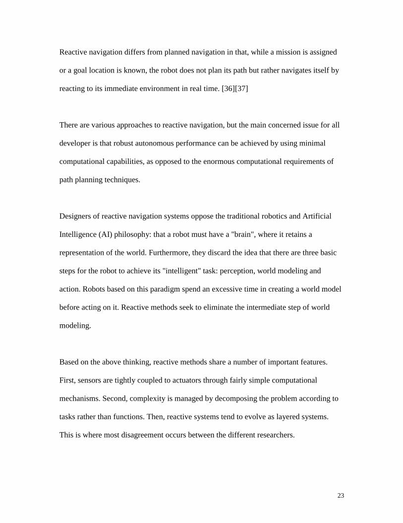
Reactive navigation differs from planned navigation in that, while a mission is assigned
or a goal location is known, the robot does not plan its path but rather navigates itself by
reacting to its immediate environment in real time. [36][37]
There are various approaches to reactive navigation, but the main concerned issue for all
developer is that robust autonomous performance can be achieved by using minimal
computational capabilities, as opposed to the enormous computational requirements of
path planning techniques.
Designers of reactive navigation systems oppose the traditional robotics and Artificial
Intelligence (AI) philosophy: that a robot must have a "brain", where it retains a
representation of the world. Furthermore, they discard the idea that there are three basic
steps for the robot to achieve its "intelligent" task: perception, world modeling and
action. Robots based on this paradigm spend an excessive time in creating a world model
before acting on it. Reactive methods seek to eliminate the intermediate step of world
modeling.
Based on the above thinking, reactive methods share a number of important features.
First, sensors are tightly coupled to actuators through fairly simple computational
mechanisms. Second, complexity is managed by decomposing the problem according to
tasks rather than functions. Then, reactive systems tend to evolve as layered systems.
This is where most disagreement occurs between the different researchers.

24
Chapter 4.
ROBOT VISION ALGORITHMS AND
TECHNIQUES
4.1. Introduction
The field of robot vision can be thought of as the application of computer vision
techniques to industrial automation. Although computer vision programs produce the
desired result, every successful vision application can be traced back to a thorough
understanding of the fundamental science of imaging.
The new machine vision industry that is emerging is already generating millions of
dollars per year in thousands of successful applications. Machine vision is becoming
established as a useful tool for industrial automation where the goal of 100% inspection
of manufactured parts during production is becoming a reality. Robot vision has now
been an active area of research for more than 35 years and it is gradually being
introduced for the real world application. [38]
4.2. Robot vision hardware component

25
A robot vision system consists of hardware and software components. The basic
hardware components consist of a light source, a solid state camera and lens, and a vision
processor. The usual desired output is data that is used to make an inspection decision or
permit a comparison with other data. The key considerations for image formation are
lighting and optics.
One of the first considerations in a robot vision application is the type illumination to be
used. Natural, or ambient, lighting is always available but rarely sufficient. Point, line,
or area lighting sources may be used as an improvement over ambient light. Spectral
considerations should be taken into account in order to provide a sufficiently high
contrast between the objects and background. Additionally, polarizing filters may be
required to reduce glare, or undesirable spectral reflections. If a moving object is
involved, a rapid shutter or strobe illumination can be used to capture an image without
motion blur. To obtain an excellent outline of an object’s boundary, back lighting can
provide an orthogonal projection used to silhouette an object. Line illumination,
produced with a cylindrical lens, has proven useful in many vision systems. Laser
illumination must be used with proper safety precautions, since high intensity point
illumination of the retina can cause permanent damage.
Another key consideration in imaging is selecting the appropriate camera and optics.
High quality lenses must be selected for proper field of view and depth of field;
automatic focus and zoom controls are available. Cameras should be selected based on

26
scanning format, geometric precision, stability, bandwidth, spectral response, signal to
noise ratio, automatic gain control, gain and offset stability, and response time. A shutter
speed or frame rate greater than one-thirtieth or one-sixtieth of a second should be used.
In fact, the image capture or digitization unit should have the capability of capturing an
image in one frame time. In addition, for camera positioning, the position, pan and tilt
angles can be servo controlled. Robot-mounted cameras are used in some applications.
Fortunately, since recent advances in solid state technology, solid state cameras are now
available at dramatically lower cost than previously.
4.3. Image functions and characteristics
As mentioned by Wagner [39], in manufacturing, human operators have traditionally
performed the task of visual inspection. Robot vision for automatic inspection provides
relief to workers from the monotony of routine visual inspection, alleviates the problems
due to lack of attentiveness and diligence, and in some cases improves overall safety.
Robot vision can even expand the range of human vision in the following ways:
• By improving resolution from optical to microscopic or electron microscopic;
• Extending the useful spectrum from the visible to the x-ray and infrared or the entire
electromagnetic range; improving sensitivity to the level of individual photons;
• Enhancing color detection from just red, green and blue spectral bands to detecting
individual frequencies;

27
}1,1,0;1,...,1,0:),({ ����� NyNxyxfI
• Improving time response from about 30 frames per second to motion stopping strobe-
lighted frame rates or very slow time lapse rates;
• And, modifying the point of view from the limited perspective of a person's head to
locations like Mars, the top of a fixture, under a conveyor or inside a running engine.
Another strength of robot vision systems is the ability to operate consistently,
repetitively, and at a high rate of speed. In addition, robot vision system components
with proper packaging, especially solid state cameras, can even be used in hostile
environments, such as outer space or in a high radiation hot cell. They can even measure
locations in three dimensions or make absolute black and white or color measurements,
while humans can only estimate relative values.
The limitations of robot vision are most apparent when attempting to do a task that is
either not fully defined or that requires visual learning and adaptation. Clearly it is not
possible to duplicate all the capabilities of the human with a robot vision system. Each
process and component of the robot vision system must be carefully selected, designed,
interfaced and tested. Therefore, tasks requiring flexibility, adaptability, and years of
training in visual inspection are still best left to humans.
Robot vision refers to the science, hardware and software designed to measure, record,
process and display spatial information. In the simplest two-dimensional case, a digital
black and white image function, I, is defined as:
(1)

28
Each element of the image f (x, y) may be called a picture element or pixel. The value of
the function f (x, y) is its gray level value, and the points where it is defined are called its
domain, window or mask.
The computer image is always quantitized in both spatial and gray scale coordinates. The
effects of spatial resolution are shown in Figure 2.
Figure 2. Image at various spatial resolutions

29
The gray level function values are quantitized to a discrete range so that they can be
stored in computer memory. A common set of gray values might range from zero to 255
so that the value may be stored in an 8-bit byte. Usually zero corresponds to dark and
255 to white. The one bit, or binary, image shows only 2 shades of gray, black for 0 and
white for 1. The binary image is used to display the silhouette of an object if the
projection is nearly orthographic. Another characteristic of such an image is the
occurrence of false contouring. In this case, contours may be produced by coarse
quantization that are not actually present in the original image. As the number of gray
shades is increased, we reach a point where the differences are indistinguishable. A
conservative estimate for the number of gray shades distinguishable by the normal human
viewer is about 64. However, changing the viewing illumination can significantly
increase this range.
Figure 3. A Digitized Image
In order to illustrate a simple example of a digital image, consider a case where a
digitizing device, like an optical scanner, is required to capture an image of 8 by 8 pixels
9 9 9 0 0 9 9 9
9 9 0 0 0 0 9 9
9 9 0 0 0 0 9 9
0 9 9 0 0 9 9 0
0 9 9 0 0 9 9 0
0 0 9 9 9 9 0 0
0 0 9 9 9 9 0 0
0 0 0 9 9 0 0 0
30
which represent the letter ‘V’. If the lower intensity value is zero and higher intensity
value is nine, then the digitized image we expected should look like Figure 3. This
example illustrates how numbers can be assigned to represent specific characters.
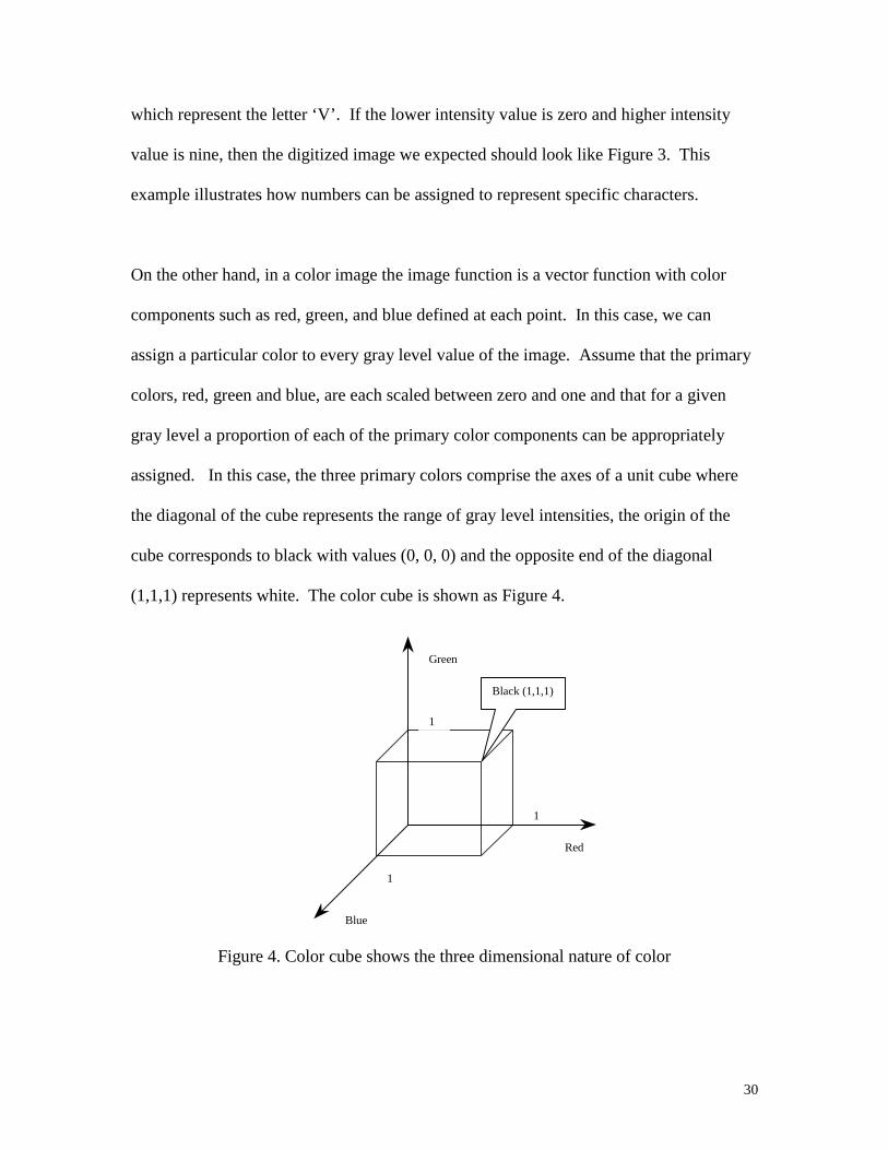
On the other hand, in a color image the image function is a vector function with color
components such as red, green, and blue defined at each point. In this case, we can
assign a particular color to every gray level value of the image. Assume that the primary
colors, red, green and blue, are each scaled between zero and one and that for a given
gray level a proportion of each of the primary color components can be appropriately
assigned. In this case, the three primary colors comprise the axes of a unit cube where
the diagonal of the cube represents the range of gray level intensities, the origin of the
cube corresponds to black with values (0, 0, 0) and the opposite end of the diagonal
(1,1,1) represents white. The color cube is shown as Figure 4.
Figure 4. Color cube shows the three dimensional nature of color
Red
Green
Blue
Black (1,1,1)
1
1
1

31
��
��
�
��
�
�
),,,,(
),,,,(
),,,,(
�
�
�
tzyxb
tzyxg
tzyxr
Colorimage
In general, a three dimensional color image function at a fixed time and with a given
spectral illumination may be written as a three dimensional vector in which each
component is a function of space, time and spectrum:
(2)
Images may be formed and processed through a continuous spatial range using optical
techniques. However, robot vision refers to digital or computer processing of the spatial
information. Therefore, the range of the spatial coordinates will be discrete values. The
necessary transformation from a continuous range to the discrete range is called
sampling, and it is usually performed with a discrete array camera or the discrete array of
photoreceptors of the human eye.
The viewing geometry is also an important factor. Surface appearance can vary from
diffuse to specular with quite different images. Lambert's law for diffuse surface
reflection surfaces demonstrates that the angle between the light source location and the
surface normal is most important in determining the amount of reflected. For specula
reflection both the angle between the light source and surface normal and the angle
between the viewer and surface normal are important in determining the appearance of
the reflected image.
32
4.4. Image processing techniques
4.4.1. Frequency Space Analysis
Since an image can be described as a spatial distribution of density in a space of one, two
or three dimensions, it may be transformed and represented in a different way in another
space. One of the most important transformations is the Fourier transform. Historically,
computer vision may be considered a new branch of signal processing, an area where
Fourier analysis has had one of its most important applications. Fourier analysis gives us
a useful representation of a signal because signal properties and basic operations, like
linear filtering and modulations, are easily described in the Fourier domain. A common
example of Fourier transforms can be seen in the appearance of stars. A star looks like a
small point of twinkling light. However, the small point of light we observe is actually
the far field Fraunhoffer diffraction pattern or Fourier transform of the image of the star.
The twinkling is due to the motion of our eyes. The moon image looks quite different
since we are close enough to view the near field or Fresnel diffraction pattern.
While the most common transform is the Fourier transform, there are also several closely
related transforms. The Hadamard, Walsh, and discrete cosine transforms are used in the
area of image compression. The Hough transform is used to find straight lines in a binary
image. The Hotelling transform is commonly used to find the orientation of the
maximum dimension of an object [40].
33
F u f x e dxiu x( ) ( )� �
��
�
�
F u v f x y e dxdy
f x y F u v e du dv
i u x vy
i u x vy
( , ) ( , )
( , ) ( , )
( )
( )
�
�
� �
��
�
�
��
�
��
��
2
2
�
�
F u vN
f x y e
f x y F u v e
i
Nu x vy
y
N
x
N
i
Nu x vy
v
N
u
N
( , ) ( , )
( , ) ( , )
( )
( )
�
�
� �
�
�
�
�
�
�
�
�
�
��
��
12
2
0
1
0
1
2
0
1
0
1
�
�
Fourier transform
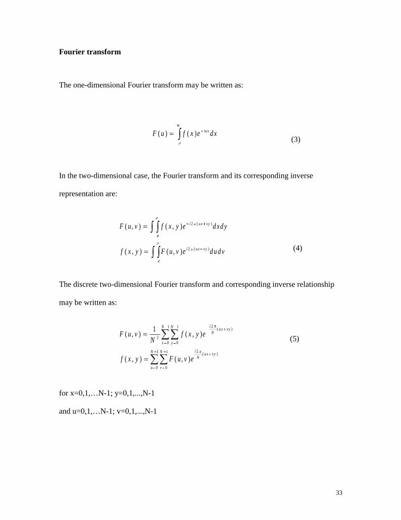
The one-dimensional Fourier transform may be written as:
(3)
In the two-dimensional case, the Fourier transform and its corresponding inverse
representation are:
(4)
The discrete two-dimensional Fourier transform and corresponding inverse relationship
may be written as:
(5)
for x=0,1,…N-1; y=0,1,...,N-1
and u=0,1,…N-1; v=0,1,...,N-1

34
4.4.2. Image Enhancement
Image enhancement techniques are designed to improve the quality of an image as
perceived by a human [40]. Some typical image enhancement techniques include gray
scale conversion, histogram, color composition, etc. The aim of image enhancement is to
improve the interpretability or perception of information in images for human viewers, or
to provide `better' input for other automated image processing techniques.
Histograms
The simplest types of image operations are point operations, which are performed
identically on each point in an image. One of the most useful point operations is based
on the histogram of an image.
Histogram Processing
A histogram of the frequency that a pixel with a particular gray-level occurs within an
image provides us with a useful statistical representation of the image.
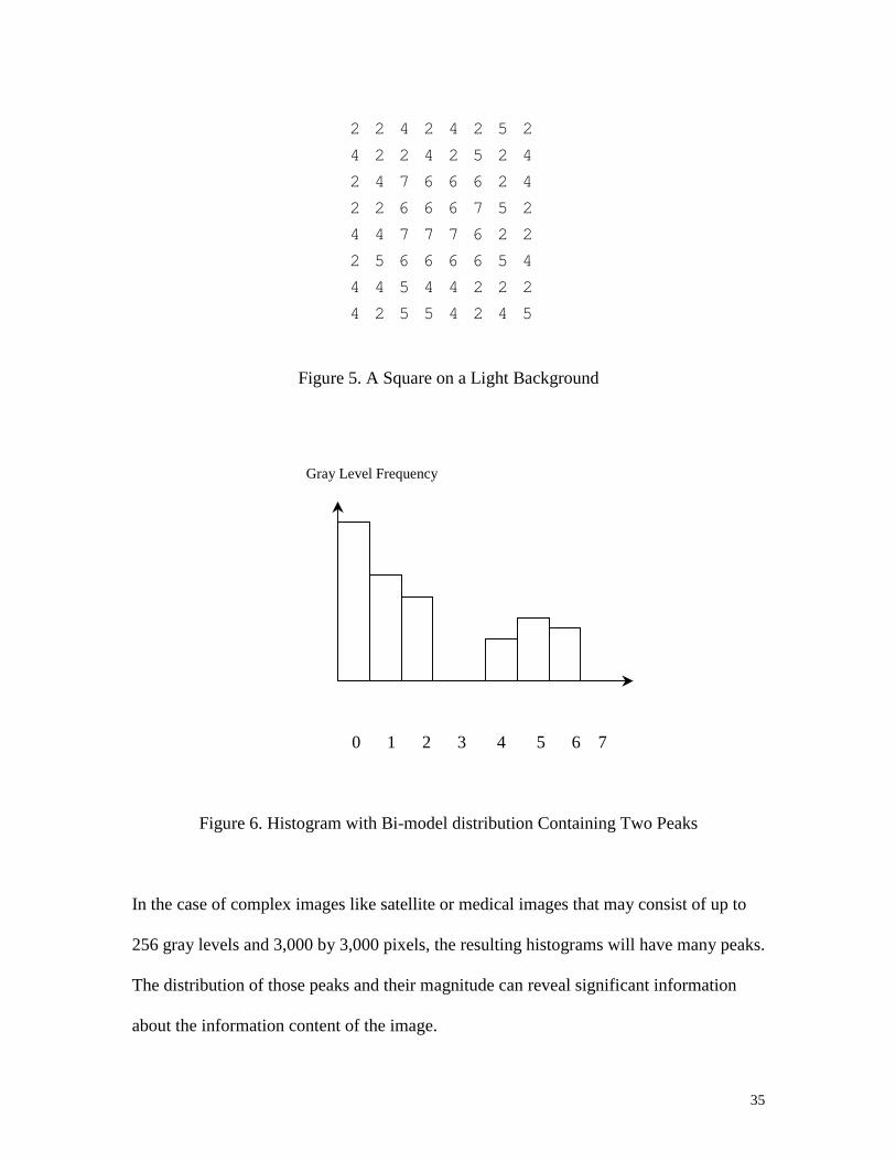
Consider the image shown in Figure 5 as an example. It represents a square on a light
background. The object is represented by gray levels greater than 4. Figure 6 shows its
histogram, which consists of two peaks.
35
Figure 5. A Square on a Light Background
0 1 2 3 4 5 6 7
Figure 6. Histogram with Bi-model distribution Containing Two Peaks
In the case of complex images like satellite or medical images that may consist of up to
256 gray levels and 3,000 by 3,000 pixels, the resulting histograms will have many peaks.
The distribution of those peaks and their magnitude can reveal significant information
about the information content of the image.
2 2 4 2 4 2 5 2
4 2 2 4 2 5 2 4
2 4 7 6 6 6 2 4
2 2 6 6 6 7 5 2
4 4 7 7 7 6 2 2
2 5 6 6 6 6 5 4
4 4 5 4 4 2 2 2
4 2 5 5 4 2 4 5
Gray Level Frequency
36
Histogram Equalization
Although it is not generally the case in practice, ideally our image histogram should be
distributed across the range of gray scale values as a uniform distribution. The
distribution can be dominated by a few values spanning only a limited range. Statistical
theory shows that using a transformation function equal to the cumulative distribution of
the gray level intensities in the image enables us to generate another image with a gray
level distribution having a uniform density.
This transformation can be implemented by a three-step process:
(1) Compute the histogram of the image;
(2) Compute the cumulative distribution of the gray levels;
(3) Replace the original gray level intensities using the mapping determined in (2).
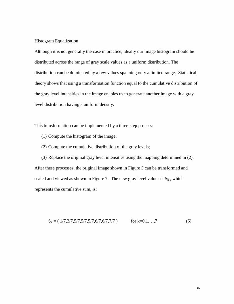
After these processes, the original image shown in Figure 5 can be transformed and
scaled and viewed as shown in Figure 7. The new gray level value set Sk , which
represents the cumulative sum, is:
Sk = ( 1/7,2/7,5/7,5/7,5/7,6/7,6/7,7/7 ) for k=0,1,…,7 (6)
37
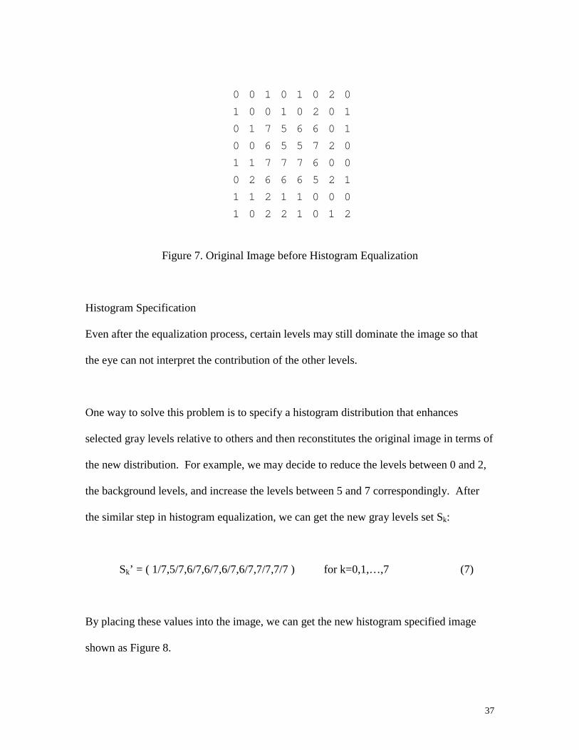
Figure 7. Original Image before Histogram Equalization
Histogram Specification
Even after the equalization process, certain levels may still dominate the image so that
the eye can not interpret the contribution of the other levels.
One way to solve this problem is to specify a histogram distribution that enhances
selected gray levels relative to others and then reconstitutes the original image in terms of
the new distribution. For example, we may decide to reduce the levels between 0 and 2,
the background levels, and increase the levels between 5 and 7 correspondingly. After
the similar step in histogram equalization, we can get the new gray levels set Sk:
Sk’ = ( 1/7,5/7,6/7,6/7,6/7,6/7,7/7,7/7 ) for k=0,1,…,7 (7)
By placing these values into the image, we can get the new histogram specified image
shown as Figure 8.
0 0 1 0 1 0 2 0
1 0 0 1 0 2 0 1
0 1 7 5 6 6 0 1
0 0 6 5 5 7 2 0
1 1 7 7 7 6 0 0
0 2 6 6 6 5 2 1
1 1 2 1 1 0 0 0
1 0 2 2 1 0 1 2

38
Figure 8. New Image after Histogram Equalization
Image Thresholding
Thresholding is the process of separating an image into different regions. This may be
based upon its gray level distribution. Figure 9 shows how an image looks after
thresholding. The percentage threshold is the percentage level between the maximum
and minimum intensity of the initial image.
Image Analysis and Segmentation
An important area of electronic image processing is the segmentation of an image into
various regions in order to separate objects from the background. These regions may
roughly correspond to objects, parts of objects, or groups of objects in the scene
represented by that image. It can also be viewed as the process of identifying edges that
1 1 5 1 5 1 6 1
5 1 1 5 1 6 1 5
1 5 7 7 7 7 1 5
1 1 7 7 7 7 6 1
5 5 7 7 7 7 6 1
1 6 7 7 7 7 1 1
5 5 6 5 5 1 1 1
5 1 6 6 5 1 5 6
39
correspond to boundaries between objects and regions that correspond to surfaces of
objects in the image. Segmentation of an image typically precedes semantic analysis of
the image. Their purposes are [41]:
� Data reduction: often the number of important features, i.e., regions and
edges, is much smaller that the number of pixels.
� Feature extraction: the features extracted by segmentation are usually “
building blocks” from which object recognition begins. These features are
subsequently analyzed based on their characteristics.
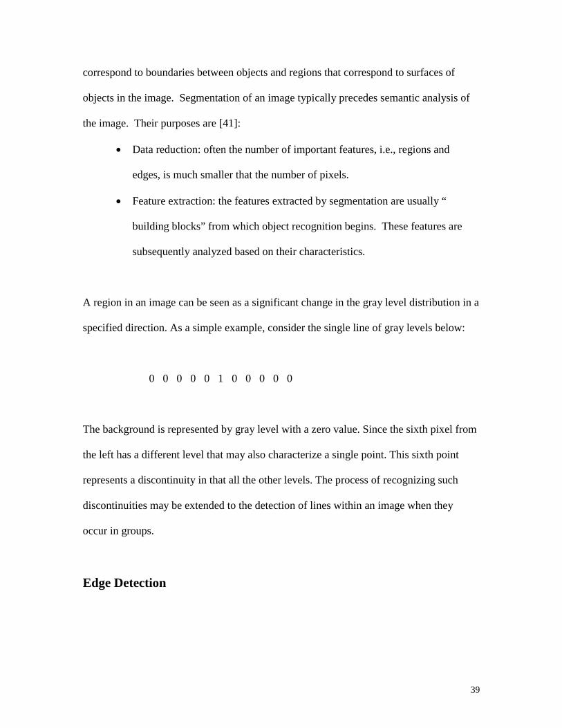
A region in an image can be seen as a significant change in the gray level distribution in a
specified direction. As a simple example, consider the single line of gray levels below:
0 0 0 0 0 1 0 0 0 0 0
The background is represented by gray level with a zero value. Since the sixth pixel from
the left has a different level that may also characterize a single point. This sixth point
represents a discontinuity in that all the other levels. The process of recognizing such
discontinuities may be extended to the detection of lines within an image when they
occur in groups.
Edge Detection
40
a a a
a a a
a a a
1 2 3
4 5 6
7 8 9
In recent years a considerable number of edge and line detecting algorithms have been
proposed, each being demonstrated to have particular merits for particular types of image.
One popular technique is called the parallel processing, template-matching method,
which involves a particular set of windows being swept over the input image in an
attempt to isolate specific edge features. Another widely used technique is called
sequential scanning, which involves an ordered heuristic search to locate a particular
feature.
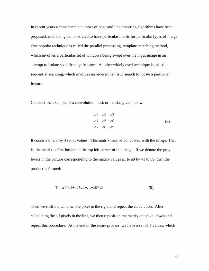
Consider the example of a convolution mask or matrix, given below.
(8)
It consists of a 3 by 3 set of values. This matrix may be convolved with the image. That
is, the matrix is first located at the top left corner of the image. If we denote the gray
levels in the picture corresponding to the matrix values a1 to a9 by v1 to v9, then the
product is formed:
T = a1*v1+a2*v2+…+a9*v9 (9)
Then we shift the window one pixel to the right and repeat the calculation. After
calculating the all pixels in the line, we then reposition the matrix one pixel down and
repeat this procedure. At the end of the entire process, we have a set of T values, which
41
G x y ex y
�
�
��( , ) �
�
�1
2 22
2 2
2
I x y I x y G x y� �
( , ) ( , ) * ( , )�
enable us determine the existence of the edge. Depending on the values used in the mask
template, various effects such as smoothing or edge detection will result.
Since edges correspond to areas in the image where the image varies greatly in
brightness, one idea would be to differentiate the image, looking for places where the
magnitude of the derivative is large. The only drawback to this approach is that
differentiation enhances noise. Thus, it needs to be combined with smoothing.
Smoothing using Gaussians
One form of smoothing the image is to convolve the image intensity with a Gaussian
function. Let us suppose that the image is of infinite extent and that the image intensity is
I (x, y). The Gaussian is a function of the form
(10)
The result of convolving the image with this function is equivalent to low pass filtering
the image. The higher the sigma, the greater the low pass filter’s effect. The filtered
image is
(11)

42
I x y I x y G x y� �
( , ) ( , ) * ( , )�
��
�xe
x y
2 22
2 2
2
��
�
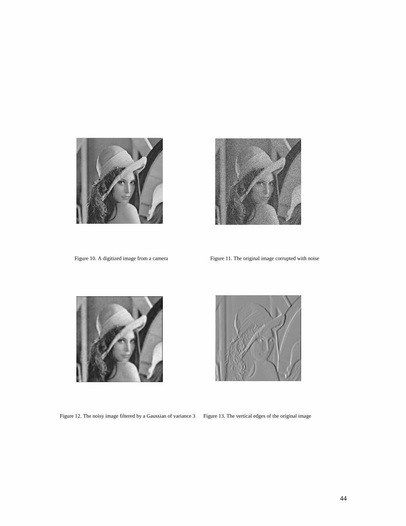
One effect of smoothing with a Gaussian function is to reduce the amount of noise,
because of the low pass characteristic of the Gaussian function. Figure 11 shows the
image with noise added to the original Figure 10.
Figure 12 shows the image filtered by a low pass Gaussian function with �= 3.
Vertical Edges
To detect vertical edges we first convolve with a Gaussian function and then differentiate
(12)
the resultant image in the x direction. This is the same as convolving the image with the
derivative of the Gaussian function in the x-direction that is
(13)
Then, one marks the peaks in the resultant images that are above a prescribed threshold as
edges (the threshold is chosen so that the effects of noise are minimized). The effect of
doing this on the image of Figure 21 is shown in Figure 13.
43
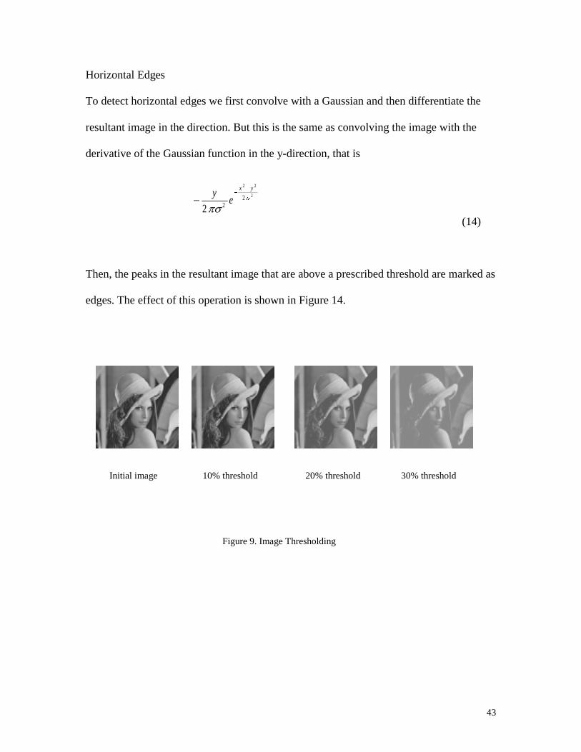
Horizontal Edges
To detect horizontal edges we first convolve with a Gaussian and then differentiate the
resultant image in the direction. But this is the same as convolving the image with the
derivative of the Gaussian function in the y-direction, that is
(14)
Then, the peaks in the resultant image that are above a prescribed threshold are marked as
edges. The effect of this operation is shown in Figure 14.
Initial image 10% threshold 20% threshold 30% threshold
Figure 9. Image Thresholding
��
�ye
x y
2 22
2 2
2
��
�
44
Figure 10. A digitized image from a camera Figure 11. The original image corrupted with noise
Figure 12. The noisy image filtered by a Gaussian of variance 3 Figure 13. The vertical edges of the original image

45
Figure 14. The horizontal edges of the original image Figure 15. The magnitude of the gradient
Figure 16. Thresholding of the peaks of the magnitude of the gradient Figure 17. Edges of the original image
46
R R R� �12
22
Canny edges detector
To detect edges at an arbitrary orientation one convolves the image with the convolution
kernels of vertical edges and horizontal edges. Call the resultant images R1(x,y) and
R2(x,y). Then form the square root of the sum of the squares.
(17)
This edge detector is known as the Canny edge detector, as shown in Figure 15, which
was proposed by (Canny and Haralick) in their 1984 papers. Now set the thresholds in
this image to mark the peaks as shown in Figure 16. The result of this operation is shown
in Figure 17.
4.4.3. Three Dimensional—Stereo
The two-dimensional digital images can be thought of as having gray levels that are a
function of two spatial variables. The most straightforward generalization to three
dimensions would have us deal with images having gray levels that are a function of
three spatial variables. The more common examples are the three-dimensional images of
transparent microscope specimens or larger objects viewed with X-ray illumination. In
these images, the gray level represents some local property, such as optical density per
millimeter of path length.

47
Most humans experience the world as three-dimensional. In fact, most of the two-
dimensional images we see have been derived from this three-dimensional world by
camera systems that employ a perspective projection to reduce the dimensionality from
three to two [41].
Spatially Three-dimensional Image
Consider a three-dimensional object that is not perfectly transparent, but allows light to
pass through it. We can think of a local property that is distributed throughout the object
in three dimensions. This property is the local optical density.
CAT Scanners
Computerized Axial Tomography ( CAT ) is an X-ray technique that produces three-
dimensional images of a solid object.
Stereometry
Stereometry is the technique of deriving a range image from a stereo pair of brightness
images. It has long been used as a manual technique for creating elevation maps of the
earth’s surface.
Stereoscopic Display
If it is possible to compute a range image from a stereo pair, then it should be possible to
generate a stereo pair given a single brightness image and a range image. In fact, this

48
technique makes it possible to generate stereoscopic displays that give the viewer a
sensation of depth.
Shaded Surface Display
By modeling the imaging system, we can compute the digital image that would result if
the object existed and if it were digitized by conventional means. Shaded surface display
grew out of the domain of computer graphics and has developed rapidly in the past few
years.
4.5. Image recognition and decisions
4.5.1. Neural Networks
Artificial neural networks can be used in image processing applications. Initially inspired
by biological nervous systems, the development of artificial neural networks has more
recently been motivated by their applicability to certain types of problem and their
potential for parallel-processing implementations.
Biological Neurons
There are about a hundred billion neurons in the brain, and they come in many different
varieties, with a highly complicated internal structure. Since we are more interested in
large networks of such units, we will avoid a great level of detail, focusing instead on

49
a f a w wi j ijj
N
� ��
�( )1
0
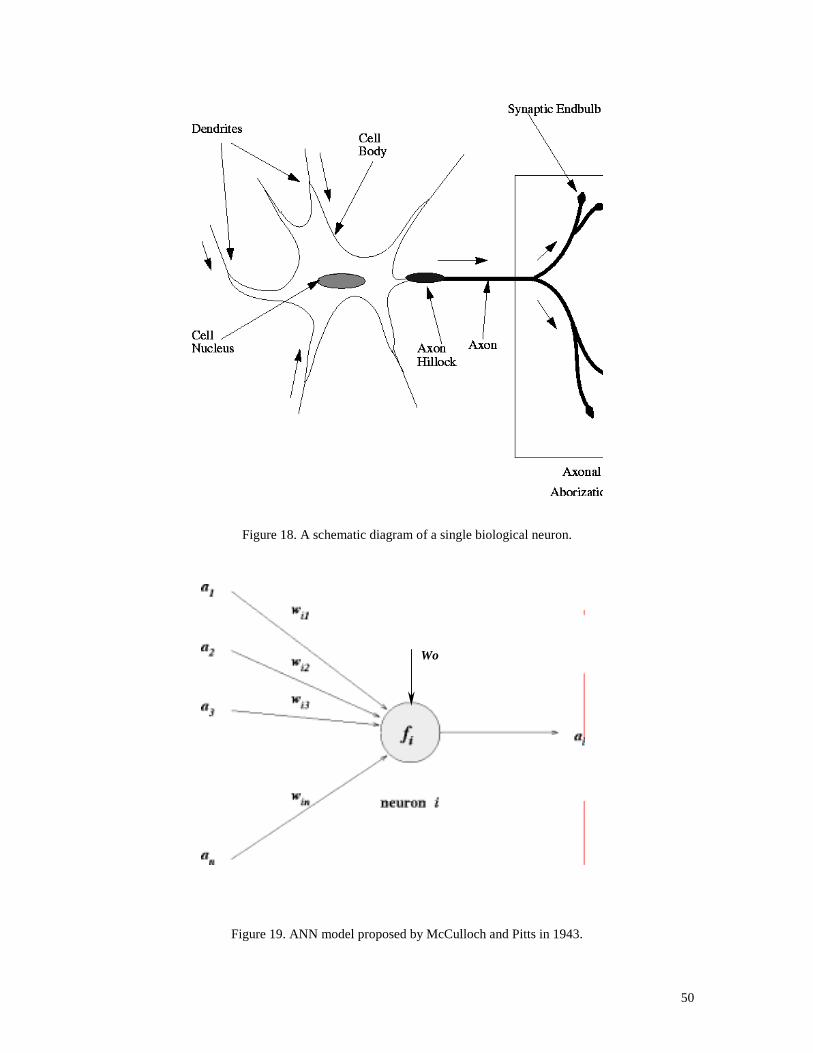
their salient computational features. A schematic diagram of a single biological neuron is
shown in Figure 18.
The cells at the neuron connections, or synapses, receive information in the form of
electrical pulses from the other neurons. The synapses connect to the cell inputs, or
dendrites, and form an electrical signal output of the neuron is carried by the axon. An
electrical pulse is sent down the axon, or the neuron “fires,” when the total input stimuli
from all of the dendrites exceeds a certain threshold. Interestingly, this local processing
of interconnected neurons results in self-organized emergent behavior.
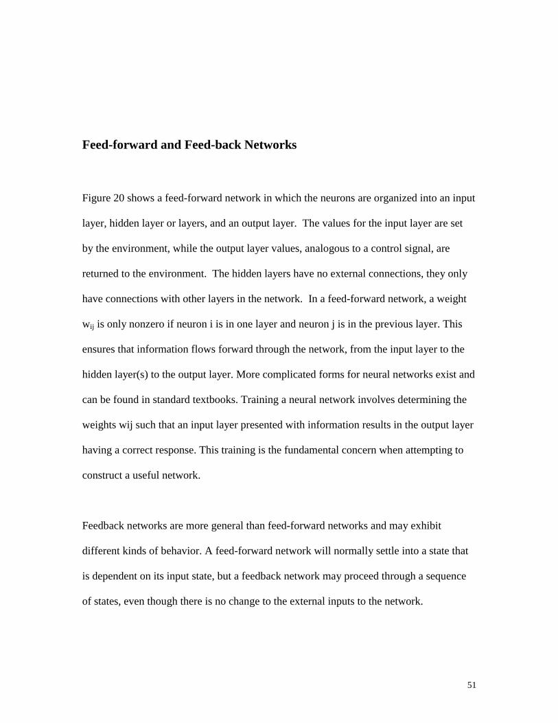
Artificial Neuron Model
The most commonly used neuron model, depicted in Figure 19, is based on the model
proposed by McCulloch and Pitts in 1943. In this model, each neuron's input, a1-an, is
weighted by the values w1 –win. A bias, or offset, in the node is characterized by an
additional constant input W0. The output, ai, is obtained in terms of the equation:
(17)
50
Figure 18. A schematic diagram of a single biological neuron.
Figure 19. ANN model proposed by McCulloch and Pitts in 1943.
Wo
51
Feed-forward and Feed-back Networks
Figure 20 shows a feed-forward network in which the neurons are organized into an input
layer, hidden layer or layers, and an output layer. The values for the input layer are set
by the environment, while the output layer values, analogous to a control signal, are
returned to the environment. The hidden layers have no external connections, they only
have connections with other layers in the network. In a feed-forward network, a weight
wij is only nonzero if neuron i is in one layer and neuron j is in the previous layer. This
ensures that information flows forward through the network, from the input layer to the
hidden layer(s) to the output layer. More complicated forms for neural networks exist and
can be found in standard textbooks. Training a neural network involves determining the
weights wij such that an input layer presented with information results in the output layer
having a correct response. This training is the fundamental concern when attempting to
construct a useful network.
Feedback networks are more general than feed-forward networks and may exhibit
different kinds of behavior. A feed-forward network will normally settle into a state that
is dependent on its input state, but a feedback network may proceed through a sequence
of states, even though there is no change to the external inputs to the network.

52
Figure 20. Feed-forward neural network
4.5.2. Supervised Learning and Unsupervised Learning
Image recognition and decision-making is a process of discovering, identifying and
understanding patterns that are relevant to the performance of an image-based task. One
of the principal goals of image recognition by computer is to endow a machine with the
capability to approximate, in some sense, a similar capability in human beings. For
example, in a system that automatically reads images of typed documents, the patterns of
interest are alphanumeric characters, and the goal is to achieve character recognition
accuracy that is as close as possible to the superb capability exhibited by human beings
for performing such tasks.
53
Image recognition systems can be designed and implemented for limited operational
environments. Research in biological and computational systems is continually
discovering new and promising theories to explain human visual cognition. However, we
do not yet know how to endow these theory and application with a level of performance
that even comes close to emulating human capabilities in performing general image
decision functionality. For example, some machines are capable of reading printed,
properly formatted documents at speeds that are orders of magnitude faster that the speed
that the most skilled human reader could achieve. However, systems of this type are
highly specialized and thus have little extendibility. That means that current theoretic
and implementation limitations in the field of image analysis and decision-making imply
solutions that are highly problem dependent.
Different formulations of learning from an environment provide different amounts and
forms of information about the individual and the goal of learning. We will discuss two
different classes of such formulations of learning.
Supervised Learning
For supervised learning, "training set” of inputs and outputs is provided. The weights
must then be determined to provide the correct output for each input. During the training
process, weights are adjusted to minimize the difference between the desired and actual
outputs for each input pattern.
54
If the association is completely predefined, it is easy to define an error metric, for
example mean-squared error, of the associated response. This in turn gives us the
possibility of comparing the performance with the predefined responses (the
“supervision”), changing the learning system in the direction in which the error
diminishes.
Unsupervised Learning
The network is able to discover statistical regularities in its input space and can
automatically develop different modes of behavior to represent different classes of inputs.
In practical applications, some “labeling” is required after training, since it is not known
at the outset which mode of behavior will be associated with a given input class. Since
the system is given no information about the goal of learning, all that is learned is a
consequence of the learning rule selected, together with the individual training data. This
type of learning is frequently referred to as self-organization.
A particular class of unsupervised learning rule which has been extremely influential is
Hebbian Learning (Hebb, 1949). The Hebb rule acts to strengthen often-used pathways in
a network, and was used by Hebb to account for some of the phenomena of classical
conditioning.
Primarily some type of regularity of data can be learned by this learning system. The
associations found by unsupervised learning define representations optimized for their
55
information content. Since one of the problems of intelligent information processing
deals with selecting and compressing information, the role of unsupervised learning
principles is crucial for the efficiency of such intelligent systems.
4.6. Future development of robot vision
Although image processing has been successfully applied to many industrial applications,
there are still many definitive differences and gaps between robot vision and human
vision. Past successful applications have not always been attained easily. Many difficult
problems have been solved one by one, sometimes by simplifying the background and
redesigning the objects. Robot vision requirements are sure to increase in the future, as
the ultimate goal of robot vision research is obviously to approach the capability of the
human eye. Although it seems extremely difficult to attain, it remains a challenge to
achieve highly functional vision systems.
The narrow dynamic range of detectable brightness is the biggest cause of difficulty in
image processing. A novel sensor with a wide detection range will drastically change the
aspect of image processing. As microelectronics technology progresses, three-
dimensional compound sensor LSIs are also expected, to which at least the preprocessing
capability will be provided.

56
As to image processors themselves, the local-parallel pipelined processor will be further
improved to proved higher processing speeds. At the same time, the multiprocessor
image processor will be applied in industry when the key-processing element becomes
more widely available. The image processor will become smaller and faster, and will
have new functions, in response to the advancement of semiconductor technology, such
as progress in system-on-chip configuration and wafer-scale integration. It may also be
possible to realize 1-chip intelligent processors for high-level processing, and to combine
these with 1-chip rather low-level image processors to achieve intelligent processing,
such as knowledge-based or model-based processing. Based on these new developments,
image processing and the resulting robot vision are expected to generate new values not
merely for industry but also for all aspects of human life [42].

57
Chapter 5.
MOBILE ROBOT SYSTEM DESIGN AND
VISION-BASED NAVIGATION SYSTEM
5.1. Introduction
Perception, vehicle control, obstacle avoidance, position location, path planning, and
navigation are generic functions which are necessary for an intelligent autonomous
mobile robot. Consider the AGV equipped with ultrasonic sensors. Given a particular set
of sonar values, we could make variously hypotheses that an object is on the right or on
the left of the robot. Depending upon the orientation information, the robot may then
move straight ahead or turn to the left or right. To avoid the difficulty in modeling the
sensor readings under a unified statistical model, the previous robot, Bearcat I, used a
rule-based fusion algorithm for the motion control. This algorithm does not need an
explicit analytical model of the environment. Expert knowledge of the sensor and robot
and prior knowledge about the environment is used in the design of the location strategy
and obstacle avoidance. After some experimentation, the rules used in control are
relatively simple, such as:
1. If the sonar reading is greater than the maximum value, then ignore the sonar input
and use vision system to guide the robot.
58
2. If the sonar input is greater than 3 feet and less than 6 feet, then check the table and
get the steering angle.
By using these simple rules, the robot is under the control of a different sub-system. The
major components of this AGV include: vision guidance system, speed and steering
control system, obstacle avoidance system, safety and braking system, power unit, and
the supervisor control PC.
5.2. System Design and Development
Sensor System
The sensor system is based on a micro-controller interfaced with one rotating ultrasonic
transducers, the vision system, and encoders.
The sensor adaptive capabilities of a mobile robot depend upon the fundamental analytical
and architectural designs of the sensor systems used. The major components of the robot
include vision guidance system, steering control system, obstacle avoidance system,
speed control, safety and braking system, power unit and the supervisor control PC. The
system block diagram is shown in Figure 21.
59
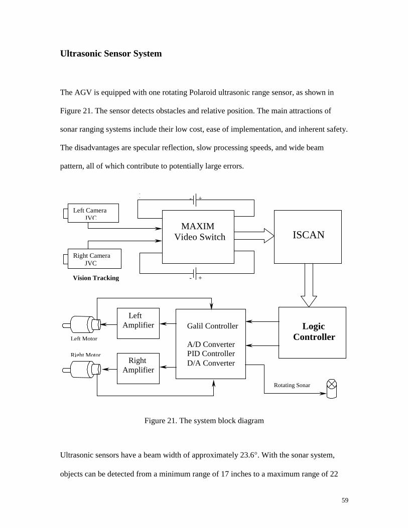
Ultrasonic Sensor System
The AGV is equipped with one rotating Polaroid ultrasonic range sensor, as shown in
Figure 21. The sensor detects obstacles and relative position. The main attractions of
sonar ranging systems include their low cost, ease of implementation, and inherent safety.
The disadvantages are specular reflection, slow processing speeds, and wide beam
pattern, all of which contribute to potentially large errors.
Figure 21. The system block diagram
Ultrasonic sensors have a beam width of approximately 23.6�. With the sonar system,
objects can be detected from a minimum range of 17 inches to a maximum range of 22
Left CameraJVC
Right Camera JVC
MAXIM Video Switch ISCAN
Logic Controller
Galil Controller
A/D Converter PID Controller D/A Converter
LeftAmplifier
RightAmplifier
Vision Tracking - +
- +
Left Motor
Right Motor
Rotating Sonar
60
feet with a 30-degree resolution. The ultrasonic sensors are also dependent upon the
texture of the reflecting surface.
Electrocraft Encoder for Motion Measurement
Encoders are widely used for applications involving measurement of linear or angular
position, velocity, and direction of movement [43]. The AGV equipped with Electrocraft
encoders with 4096 counts/revolution. Encoder is sensitive to external disturbances
(slippage, uneven ground, etc.) and internal disturbances (unbalanced wheels, encoder
resolution, etc.), but it does not require an initial set-up of the environment. By using
encoders, we can determine the travel distance since C=2 r.
Visual Sensor System
Visual information is converted to electrical signals by the use of visual sensors. The
most commonly used visual sensors are cameras. Despite the fact that these cameras
posses undesirable characteristics, such as noise and distortion that frequently necessitate
readjustments, they are used because of their ease of availability and reasonable cost.
Vision sensors are critically dependent on ambient lighting conditions and their scene
analysis and registration procedures can be complex and time-consuming.
61
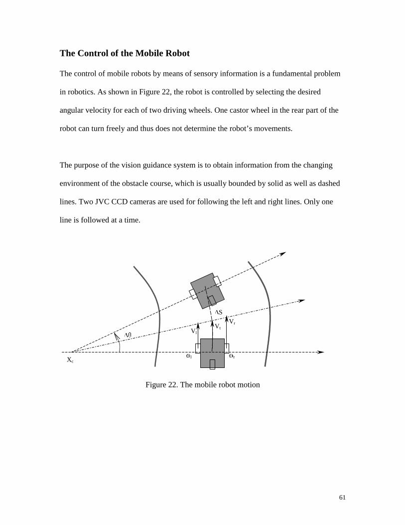
The Control of the Mobile Robot
The control of mobile robots by means of sensory information is a fundamental problem
in robotics. As shown in Figure 22, the robot is controlled by selecting the desired
angular velocity for each of two driving wheels. One castor wheel in the rear part of the
robot can turn freely and thus does not determine the robot’s movements.
The purpose of the vision guidance system is to obtain information from the changing
environment of the obstacle course, which is usually bounded by solid as well as dashed
lines. Two JVC CCD cameras are used for following the left and right lines. Only one
line is followed at a time.
Figure 22. The mobile robot motion
��
�l �r
Vl
VrVt
Xc
�S
62
X cD V
V Vw t
r l
��
*
VV V
tl r��
2
� � �� � ��
tV
Xt
V V
Dt
c
r l
w
The ISCAN image-tracking device is used for image processing. This device can find the
centroid of the brightest or darkest region in a computer controlled window and returns
the X and Y coordinates of its centroid.
5.3. Robot’s Kinematics Analysis
Figure 22 shows the robot and a typical movement generated during a fixed time step �t
when wheel angular velocities �l and �r have been selected. Then the linear velocities Vl
and Vr can be determined by �l, �r and wheel radii Rl , Rr. Let Dw be the distance
between two driving wheel, then:
(18)
where
(19)
In general, the velocities can be assumed to be constant for a short time period. As a
result, given a pair of angular velocities �l and �r, during a time �t, the robot will move
along a circular path of radius Xc, rotating through an angle:
(20)

63
� � �S X tV V
xl r� ��
� *2
And the distance is:
(21)
These equations show that specification of both �S and �� uniquely determines a
combination (Vl and Vr). This property of the robot’s kinematics is fundamental to the
function of ANN model, which will described in the following section.
5.4. Vision Guidance System and Stereo vision
Point or line tracking is achieved through the medium of a digital CCD camera. Image
processing is done by an Iscan [44] tracking device. This device finds the centroid of the
brightest or darkest region in a computer controlled window, and returns its X,Y image
coordinates as well as size information.
5.4.1. Image modeling

64
I
U
V
S
T
x
y
z* �
�
�
���
�
�
����
�
�
����
�
�
����
1
The camera is modeled by its optical center C and its image plane � (Figure 23). A point
P(x, y, z) in the observed space projects onto the camera retina at an image point I. Point
I is the intersection of the line PC with the plane �.
Figure 23. Camera Image Model
The transformation from P to I is modeled by a linear transformation T in homogeneous
coordinates. Letting I* = (U,V,S)T be the projective coordinate of I and (x,y,z)T be the
coordinates of P, we have the relation
(22)
Where T is a 3*4 matrix, generally called the perspective matrix of the camera.
I (u,v)
P (x,y,z)
C
65
Iu
v
U S
V S��
���
�
�
��
�
/
/
� � � � � �11
434241
333231
232221
131211
VUWWYX
TTT
TTT
TTT
TTT
ZYX ��
����
�
�
����
�
�
If the line PC is parallel to the image plane �, then S=0 and the coordinates (u,v) T of the
image point I are undefined. In this case, we say that P is in the focal plane of the camera.
In the general case, S�0 and the physical image coordinates of I are defined by:
(23)
5.4.2. Mathematical Models
We can define a point in homogeneous 3-D world coordinates as:
[ X, Y, Z, W ] (24)
And a homogeneous point in 2-D image space as:
[ X, Y, W ] (25)
the transformation matrix that relates these two coordinate systems is:
(26)

66
wTZTYTXT
wVTZTYTXT
wUTZTYTXT
����
����
����
43332313
42322212
41312111
� � � � � � � �
� � � � � � � � 0
0
4342333223221312
4341333123211311
��������
��������
VTTZVTTYVTTXVTT
UTTZUTTYUTTXUTT
BAX �
� � BAAAX TT 1��
Here we have arbitrarily set the homogeneous scaling factor W=1. If we multiply out
these matrix equations, we get:
(27-29)
If we eliminate the value of w, we get two new equations:
(30-31)
If we know a point (X, Y, Z) in 3-D world coordinate space and its corresponding image
coordinates (U, V) then we can view this as a series of 2 equations in 12 unknown
transform parameters Tij . Since we get 2 equations per pair of world and image points we
need a minimum of 6 pairs of world and image points to calculate the matrix. In practice,
due to errors in the imaging system we will want to use an overdetermined system and
perform a least square fit of the data. The technique used in solving an overdetermined
system of equations
(32)
Is to calculate the pseudo-inverse matrix and solve for X:
(33)
67
5.4.3. Camera calibration
Calibration is an important issue in computer vision. A very careful calibration is needed
to obtain highly precise measurements. The calibration procedure determines the
projection parameters of the camera, as well as the transformation between the coordinate
systems of the camera and the robot.
In order to determine depth, a transformation between the camera image coordinates and
the 3-D world coordinate system being used is needed. The purpose of the camera
calibration is to determine the transformation equations that map each pixel of the range
image into Cartesian coordinates. More specifically, it is to determine the camera and
lens model parameters that govern the mathematical or geometrical transformation from
world coordinates to image coordinates based on the known 3-D control field and its
image.
To calibrate the camera, we determine the optical center, the focal length expressed in
horizontal and vertical pixels, and a 2-D to 2-D function to correct the barrel distortion
introduced by the wide-angle lens. The transformation between the coordinate systems of
the camera and of the robot (rotation and translation) is also completely measured.

68
4”
Casterwheel
Robot Centroid
x
y
Right Pan Angle
Left Pan Angle
Right wheel
10’
3’5
3’5
Ql
Qr
Left wheel
Figure 24. The model of the mobile robot in the obstacle course
The model of the mobile robot illustrating the transformation between the image and the
object is shown in Figure 24. The robot is designed to navigate between two lines that
are spaced 10 feet apart. The lines are nominally 4 inches wide but are sometimes
dashed. This requires a two-camera system design so that when a line is missing, the
robot can look to the other side via the second camera.
69
Chapter 6.
A NEURO-FUZZY METHOD FOR THE
REACTIVE NAVIGATION
6.1. Neuro-fuzzy Technology
Neural networks and fuzzy systems (or neuro-fuzzy systems), in various forms, have
been of much interest recently, particularly for the control of nonlinear processes.
Early work combining neural nets and fuzzy methods used competitive networks to
generate rules for fuzzy systems (Kosko 1992). This approach is sort of a crude version
of bi-directional counterpropagation (Hecht-Nielsen 1990) and suffers from the same
deficiencies. More recent work (Brown and Harris 1994; Kosko 1997) has been based on
the realization that a fuzzy system is a nonlinear mapping from an input space to an
output space that can be parameterized in various ways and therefore can be adapted to
data using the usual neural training methods or conventional numerical optimization
algorithms.
A neural net can incorporate fuzziness in various ways:

70
� The inputs can be fuzzy. Any garden-variety backpropogation net is fuzzy in this
sense, and it seems rather silly to call a net "fuzzy" solely on this basis, although
Fuzzy ART has no other fuzzy characteristics.
� The outputs can be fuzzy. Again, any garden-variety backpropogation net is fuzzy in
this sense. But competitive learning nets ordinarily produce crisp outputs, so for
competitive learning methods, having fuzzy output is a meaningful distinction. For
example, fuzzy c-means clustering is meaningfully different from (crisp) k-means.
Fuzzy ART does not have fuzzy outputs.
� The net can be interpretable as an adaptive fuzzy system. For example, Gaussian RBF
nets and B-spline regression models are fuzzy systems with adaptive weights and can
legitimately be called Neuro-fuzzy systems.
� The net can be a conventional NN architecture that operates on fuzzy numbers instead
of real numbers.
� Fuzzy constraints can provide external knowledge.
6.2. Fuzzy Set Definition for the Navigation System
By defining the steering angle of the mobile robot is from –30 degree to 30 degree. The
fuzzy sets could be defined as follows:
(a) The robot current angle with respected to the line direction: (Input Variable: AG)
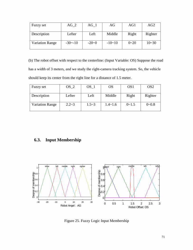
71
Fuzzy set AG_2 AG_1 AG AG1 AG2
Description Lefter Left Middle Right Righter
Variation Range -30~-10 -20~0 -10~10 0~20 10~30
(b) The robot offset with respect to the centerline: (Input Variable: OS) Suppose the road
has a width of 3 meters, and we study the right-camera tracking system. So, the vehicle
should keep its center from the right line for a distance of 1.5 meter.
Fuzzy set OS_2 OS_1 OS OS1 OS2
Description Lefter Left Middle Right Righter
Variation Range 2.2~3 1.5~3 1.4~1.6 0~1.5 0~0.8
6.3. Input Membership
Figure 25. Fuzzy Logic Input Membership
-30 -20 -10 0 10 20 30
0
0.2
0.4
0.6
0.8
1
Robot Angel : AG
Deg
ree
of m
embe
rshi
p
lefter left middle right righter
0 0.5 1 1.5 2 2.5 3
0
0.2
0.4
0.6
0.8
1
Robot Offset: OS
Deg
ree
of m
embe
rshi
p
righter right middle left lefter
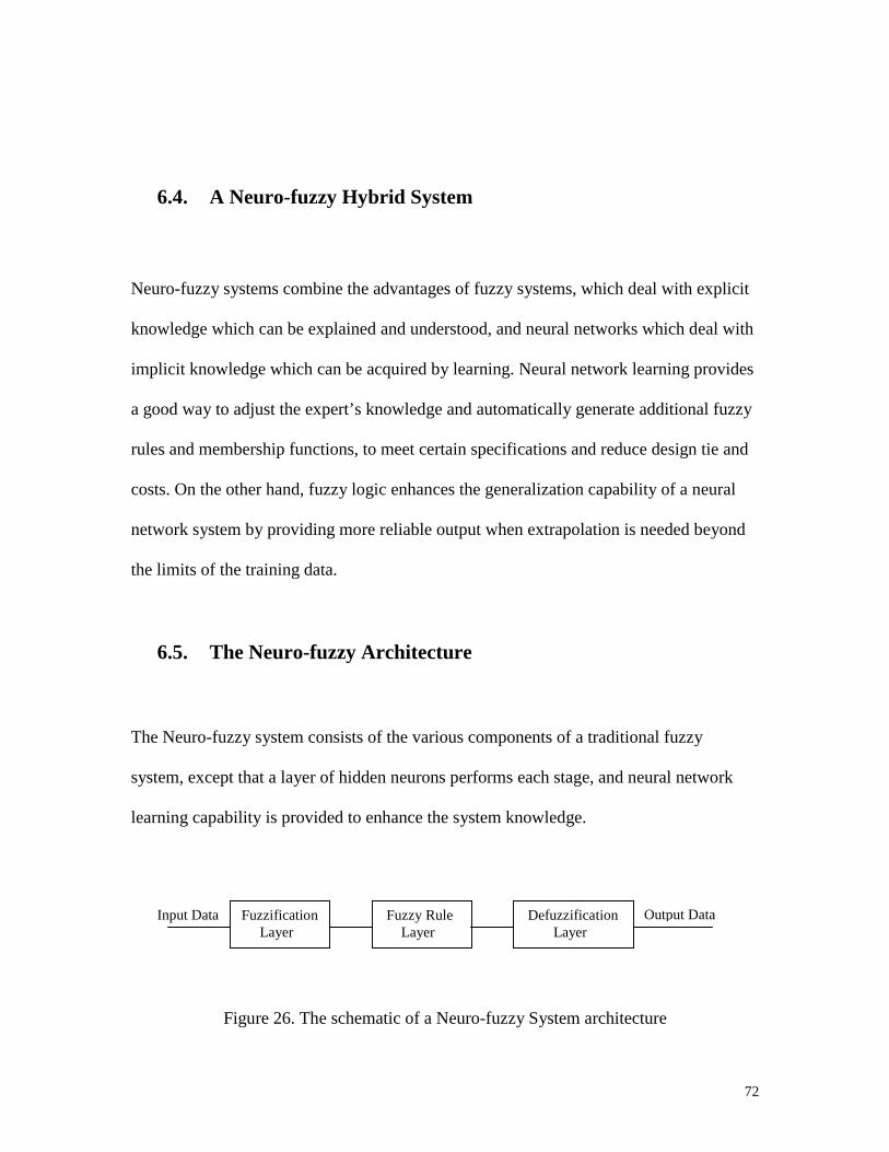
72
6.4. A Neuro-fuzzy Hybrid System
Neuro-fuzzy systems combine the advantages of fuzzy systems, which deal with explicit
knowledge which can be explained and understood, and neural networks which deal with
implicit knowledge which can be acquired by learning. Neural network learning provides
a good way to adjust the expert’s knowledge and automatically generate additional fuzzy
rules and membership functions, to meet certain specifications and reduce design tie and
costs. On the other hand, fuzzy logic enhances the generalization capability of a neural
network system by providing more reliable output when extrapolation is needed beyond
the limits of the training data.
6.5. The Neuro-fuzzy Architecture
The Neuro-fuzzy system consists of the various components of a traditional fuzzy
system, except that a layer of hidden neurons performs each stage, and neural network
learning capability is provided to enhance the system knowledge.
Figure 26. The schematic of a Neuro-fuzzy System architecture
Input Data Fuzzification Layer
Fuzzy Rule Layer
Defuzzification Layer
Output Data
73
6.6. The Implementation of Fuzzy Rules
Figure 27. shows a simple case of Neuro-fuzzy system for mobile robot navigation. A set
of navigation rules is employed in the system.
For the Right Camera Line Tracking:
Rule 1: IF Offset is RIGHT and Angle is POSITIVE THEN the Steer_Angle is ZERO
Rule 2: IF Offset is RIGHT and Angle is ZERO THEN the Steer_Angle is LEFT
Rule 3: IF Offset is RIGHT and Angle is NEGATIVE THEN the Steer_Angle is LEFT
Rule 4: IF Offset is CENTER and Angle is POSITIVE THEN the Steer_Angle is RIGHT
Rule 5: IF Offset is CENTER and Angle is ZERO THEN the Steer_Angle is ZERO
Rule 6: IF Offset is CENTER and Angle is NEGATIVE THEN the Steer_Angle is LEFT
Rule 7: IF Offset is LEFT and Angle is POSITIVE THEN the Steer_Angle is RIGHT
Rule 8: IF Offset is LEFT and Angle is ZERO THEN the Steer_Angle is RIGHT
Rule 9: IF Offset is LEFT and Angle is NEGATIVE THEN the Steer_Angle is ZERO
The value at the end of each rule represents the initial weight of the rule, and will be
adjusted to its appropriate level at the end of training. All the rules lead to three different
subjects, which is the steer direction for the mobile robot. Then three output nodes are
needed. They are TURN RIGHT, GO STRAIGHT and TURN LEFT correspondingly.
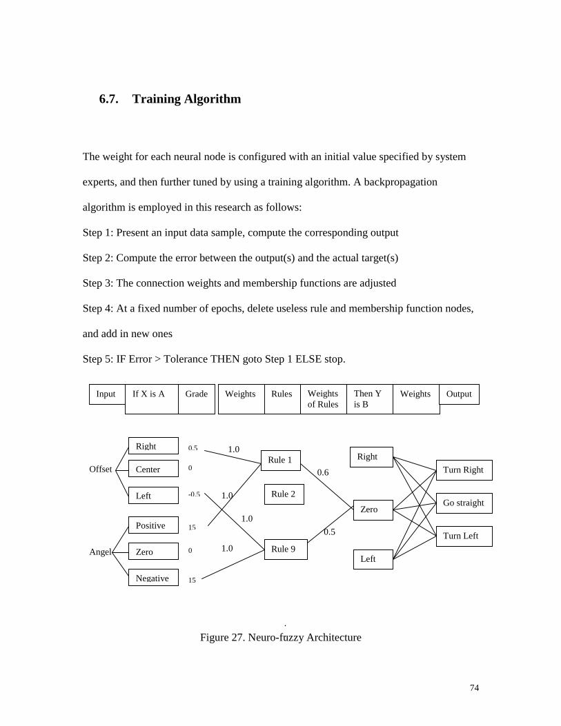
74
6.7. Training Algorithm
The weight for each neural node is configured with an initial value specified by system
experts, and then further tuned by using a training algorithm. A backpropagation
algorithm is employed in this research as follows:
Step 1: Present an input data sample, compute the corresponding output
Step 2: Compute the error between the output(s) and the actual target(s)
Step 3: The connection weights and membership functions are adjusted
Step 4: At a fixed number of epochs, delete useless rule and membership function nodes,
and add in new ones
Step 5: IF Error > Tolerance THEN goto Step 1 ELSE stop.
Figure 27. Neuro-fuzzy Architecture..
Input If X is A Grade Weights Rules Weightsof Rules
Then Yis B
Weights Output
Offset
Right
Center
Left
Angel
Positive
Zero
Negative
0.5
0
-0.5
0
15
15
Rule 1
Rule 9
1.0
1.0
1.0
1.0
Right
Zero
Left
0.6
0.5
Turn Right
Go straight
Turn Left
Rule 2

75
When the error level drops to below the user-specified tolerance, the final interconnection
weights reflect the changes in the initial fuzzy rules and membership functions. If the
resulting weight of a rule is close to zero, the rule can be safely removed from the rule
base, since it is insignificant compared to others. Also, the shape and position of the
membership functions in the Fuzzification and Defuzzification Layers can be fine-tuned
by adjusting the parameters of the neurons in these layers, during the training process.
76
Chapter 7.
CONCLUSION
The robot navigation in the outdoor environment is still a challenging job [13]. The
partially known global information makes the navigation difficult. In this research, in order
to investigate the potential of application, one path planner based on Neuro-Fuzzy was
considered. The navigation system using Neuro-Fuzzy enabled the mobile robot to move
efficiently from a known position to a specified target position without colliding with
obstacles. The basic test platform has been designed, constructed and simulated.
However, a more sophisticated algorithms and advanced control techniques need to be
investigated.
The Neuro-Fuzzy system offers the precision and learning capability of neural networks,
and yet are easy to understand like a fuzzy system. Explicit knowledge acquired from
experts can be easily incorporated into the navigation system, and implicit knowledge can
be learned from training samples to enhance the accuracy of the output. A basic case is
studied in this research. Furthermore, the modified and new rules can be extracted from a
properly trained neuro-fuzzy system, to explain how the results are derived. Some new
technologies can be developed on the Bearcat II test bed to improve the learning speed,
adjust learning and momentum rates, etc.
77
References
1. Akio Kosaka and Juiyao Pan, Purdue Experiments in Model-based Vision for
Hallway Navigation, Proceedings of workshop on Vision for Robots in IROS’95
conference, Pillsburgh, PA, 1995, pp. 87-96, 1995.
2. George. v. Wichert, Self Organizing Visual Perception for Mobile Robot
Navigation, 1st EUROMICRO Workshop on Advanced Mobile Robots
(EUROBOT'96), Kaiserslautern, Germany, 1996. http://www.rt.e-technik.th-
darmstadt.de/~georg/pubs/EUROBOT96/paper.html
3. Michaud, Francois Mataric, Maja J. , Learning From History for Adaptive Mobile
Robot Control, Proceedings of the 1998 IEEE/RSJ International Conference on
Intelligent Robots and Systems. Part 3 (of 3), Victoria, Can, Oct. 13-17, 1998, pp.
1865-1870.
4. Minato, Takashi Asada, Minoru, Environmental Change Adaptation for Mobile
Robot Navigation, Proceeding of the 1998 IEEE/RSJ International Conference on
Intelligent Robots and Systems. Part 3 (of 3), Victoria, Can, Oct. 13-17, 1998, pp.
1859-1864.
5. Mora, Thamar E. Sanchez, Edgar N., Fuzzy Logic-based Real-time Navigation
Controller for a Mobile Robot, Proceeding of the 1998 IEEE/RSJ International
Conference on Intelligent Robots and Systems. Part 1 (of 3), Victoria, Can, Oct. 13-
17, 1998, pp. 612-617.
6. Kim, Kyung-Hoon Cho, Hyung Suck, Mobile Robot Navigation Based on Optimal
Via-point Selection Method, Proceeding of the 1998 IEEE/RSJ International

78
Conference on Intelligent Robots and Systems. Part 2 (of 3), Victoria, Can, Oct. 13-
17, 1998, pp. 1242-1247.
7. Watanabe, Keigo Lzumi, Kiyotaka Tang, Jun Han, Fuhua, Rotational Control of an
Omnidirectional Mobile Robot Using a Fuzzy Servo Controller, Advanced
Robotics, Vol. 12, Issue 3, 1998, pp. 171-189.
8. Choi, Jung W. Kwon, Soon H. Lee, Hae Y. Lee, Suk G., Navigation Strategy of an
Intelligent Mobile Robot Using Fuzzy logic, Proceedings of the 1998 IEEE
International Conference on Fuzzy Systems, Part 1 of 2, Archorage, AK, USA, May
4-9, 1998, pp. 602-605.
9. Vercelli, G. Morasso, P. , Recognition and Classification of Path Features With
Self-organizing Maps During Reactive Navigation, Proceeding of the 1998
IEEE/RSJ International Conference on Intelligent Robots and Systems. Part 3 (of 3),
Victoria, Can, Oct. 13-17, 1998, pp. 1437-1442.
10. Streilein, Willian W. Gaudiano, Paolo Carpenter, Gail A., Neural Network for
Object Recognition Through Sonar on a Mobile Robot, Proceedings of the 1998
IEEE International Symposium on Intelligent Control, ISIC, Gaithersburg, MD, USA,
Sep. 14-17, 1998, pp. 271-276.
11. Dracopoulos, Dimitris C., Robot Path Palnning for Maze Navigation, Proceedings
of the 1998 IEEE International Joint Conference on Neural Networks, Part 3of 3),
Anchorage, AK, USA, May 4-9, 1998, pp. 2081-2085.
12. Zhu, Zhigang Yang, Shiqiang Shi, Dingji Xu, Guangyou, Better Road Following by
Integrating Omni-view Images and Neural Nets, Proceedings of the 1998 IEEE

79
International Joint Conference on Neural Networks, Part 2of 3), Anchorage, AK,
USA, May 4-9, 1998, pp. 974-979.
13. Cicirelli, G. Distante, C. D’Orazio, T. Attolico, G. , Learning Actions from Vision-
based Positioning in Goal-directed Navigation, Proceedings of the 1998 IEEE.RSJ
International Conference on Intelligent Robots and Systems, part 3 (of 3), Victoria,
Can, Oct. 13-17, 1998, pp. 1715-1720.
14. Kruse, E. Wahl, F.M., Camera-based Monitoring System for Mobile Robot
Guidance, Proceeding of the 1998 IEEE/RSJ International Conference on Intelligent
Robots and Systems. Part 2 (of 3), Victoria, Can, Oct. 13-17, 1998, pp.1248-1253.
15. Little, James J. Lu, Jiping Murray, Don R., Selecting Stable Image Features for Robot
Localization Using Stereo, Proceeding of the 1998 IEEE/RSJ International
Conference on Intelligent Robots and Systems. Part 2 (of 3), Victoria, Can, Oct. 13-
17, 1998, pp. 1072-1077.
16. Arsenio, Artur Ribeiro, M. Isabel, Active Range Sensing for Mobile Robot
Localization, Proceeding of the 1998 IEEE/RSJ International Conference on
Intelligent Robots and Systems. Part 2 (of 3), Victoria, Can, Oct. 13-17, 1998, pp.
1066-1071.
17. Grudic, Gregory Z. Lawrence, Peter D., Nonparametric Learning Approach to
Vision Based Mobile Robot Lacalization, Proceedings of the 1998 IEEE.RSJ
International Conference on Intelligent Robots and Systems, part 2 (of 3), Victoria,
Can, Oct. 13-17, 1998, pp. 724-729.
18. Feder, Hans Jacob S. Leonard, John J. Smith, Chris M., Adaptive Concurrent
Mapping and Localization Using Sonar, Proceeding of the 1998 IEEE/RSJ
80
International Conference on Intelligent Robots and Systems. Part 2 (of 3), Victoria,
Can, Oct. 13-17, 1998, pp. 892-898.
19. Vlassis, N.S. Papakonstantinou, G. Tsanakas, P., Dynamic Sensory Probabilistic
Maps for Mobile Robot Localization, Proceedings of the 1998 IEEE.RSJ
International Conference on Intelligent Robots and Systems, part 2 (of 3), Victoria,
Can, Oct. 13-17, 1998, pp.718-723.
20. Hiraishi, Hironori Ohwada, Hayato Mizoguchi, Fumio, Web-based Communication
and Control for Multiagent Robots, Proceedings of the 1998 IEEE.RSJ
International Conference on Intelligent Robots and Systems, part 1 (of 3), Victoria,
Can, Oct. 13-17, 1998, pp.120-125.
21. Ng, Kim C. Trivedi, Mohan M., Neuro-fuzzy Controller for Mobile Robot
Navigation and Multirobot Convoying, IEEE Transactions on Systems, Man, and
Cybernetics, Part B: Cybernetics, Vol. 28, Issue 6, 1998, IEEE, Piscataway, NJ, USA,
pp. 829-840.
22. Daxwanger, Wolfgand A. Schmidt, Guenther, Neuro-fuzzy Posture Estimation for
Visual Vehicle Guidance, Proceedings of the 1998 IEEE International Joint
Conference on Neural Networks, Part 3 (of 3), Anchorage, AK, USA, May, 4-9,
1998, pp. 2086-2091.
23. Bekey, George A., On autonomous Robots, Knowledge Engineering Review, Vol.
13, Issue 2, 1998, Cambridge Univ. Press, New York, NY, USA, pp. 143-146.
24. D.H.Hubel and T.N. Wiesel, “Receptive fields, binocular interaction and
functional architecture in the cat’s visual cortex”, J. Physiol. 160, 1962, pp. 106-
154.
81
25. Yiannis Aloimonos, Visual Navigation: From Biological Systems to Unmanned
Ground Vehicles, Lawrence Erlbaum Associates, Publishers, 1997, Mahwah, New
Jersey.
26. Paris Andreou and Adonis Charalambides, Exploring Mars Using Intelligent
Robots, http://www-dse.doc.ic.ac.uk/~nd/surprise_95/journal/vol4/pma/report.html.
27. Araujo, Rui; de Almeida, Anibal T., Learning sensor-based navigation of a real
mobile robot in unknown worlds, IEEE Transactions on Systems, Man, and
Cybernetics, Part B: Cybernetics v 29 n 2 1999 p.164-178
28. De la Escalera, A.; Moreno, L.; Salichs, M. A.; Armingol, J. M., Continuous mobile
robot localization by using structured light and a geometric map, International
Journal of Systems Science v 27 n 8 1996 p.771-782.
29. Borenstein, J.; Everett, H. R.; Feng, L.; Wehe, D., Mobile robot positioning:
sensors and techniques, Journal of Robotic Systems v 14 n 4 1997 p.231-249.
30. Janet, Jason A.; Luo, Ren C.; Kay, Michael G., Autonomous mobile robot global
motion planning and geometric beacon collection using traversability vectors,
IEEE Transactions on Robotics and Automation v 13 n 1 1997 p.132-140.
31. Premvuti, Suparerk; Wang, Jing, Relative position localizing system for multiple
autonomous mobile robots in distributed robotic system: system design and
simulation, Robotics and Autonomous Systems v 18 n 3 1996 p.319-326.
32. Betke, Margrit; Gurvits, Leonid, Mobile robot localization using landmarks, IEEE
Transactions on Robotics and Automation v 13 n 2 1997 p.251-263.
33. Borenstein, J.; Everett, H. R.; Feng, L.; Wehe, D., Mobile robot positioning:
sensors and techniques, Journal of Robotic Systems v 14 n 4 1997 p.231-249.

82
34. Zelinsky, A.; Kuniyoshi, Y., Learning to coordinate behaviors for robot
navigation, Advanced Robotics v 10 n 2 1996 p.143-159.
35. Kotani, Shinji; Nishikawa, Kazuhiro; Mori, Hideo, Empirical learning in mobile
robot navigation, Advanced Robotics v 12 n 4 1998 p.317-333.
36. Lee, David; Recce, Michael, Quantitative evaluation of the exploration
strategies of a mobile robot, International Journal of Robotics Research v 16 n 4
1997 p.413-447.
37. Matia, F.; Jimenez, Multisensor fusion: an autonomous mobile robot, A. Journal of
Intelligent and Robotic Systems: Theory & Applications v 22 n 2 1998 p.129-141.
38. Prasanthi Guda, Jin Cao, Jeannine Gailey and Ernest L. Hall, ” Fundamentals of
Machine Vision”, Handbook of Industrial Automation , Marcel Dekker, New York.
39. Gary Wagner, Now That They’re Cheap, We have to Make Them Smart, Proceedings
of the SME Applied Machine Vision ’96 Conference, Cincinnati, OH, June 3-6, 1996,
pp. 463-485.
40. E.L. Hall, Computer Image Processing and Recognition, Academic Press, 1979.
41. S. Shager, and T. Kanada, Recursive Region Segmentation by Analysis of
Histograms, Proceedings of IEEE International Conference on Acoustics, Speech,
and Signal Processing, 1982, pp. 1166-1171.
42. Masakazu Ejiri, Machine Vision: A Practical Technology for Advanced Image
Processing, Gordon and Breach Science Publishers, New York, NY, 1989, pp. 111-
115.
43. Devadas Shetty, Richard A.Kolk, Mechatronics System Design, PWS Publishing
Company, Boston, MA, 1997.

83
44. Iscan Inc., RK-446-R Video Tracking System Manual, Cambridge, Massachusets,
1993.
45. Jahann Borenstein, H.R. Everett, Liqiang Feng, Navigating Mobile Robots, A.K.
Peters, Wellesley, Massachusetts, 1996.

84
Appendix
C++ Source code for the Robot Vision and Motion Control
//***************************************************************
//Project: BearCat II Mobile Robot
//Coding: 99’ UC Robot Team
//Input Module: Vision System, Sonar Sensor System
//Output Module: Navigation and Motion Control Command
//File Name: G-Cart.cpp
//***************************************************************
#include "g-cart.h" // Header file used with this code.
#include "rotatson.h"
#include "galil.c"
#include "setpid.c" // Sets the PID values
#include "tsonar.c"
#include "galil.c"
#include "camera.c"
#include "vision.c"
#include "vis_main.c" // Vision auto mode
#include "car.c" // Starts, stops, steers and speedens the robot
#include "test_cam.c" // To test the cameras
#include "man_move.c" // To manually move the robots
#include "vis_demo.c" // To test the vision
#include "rotatson.c"
#include "ftl.c"

85
time_t first = time (NULL);
void Escape_to_exit(void);
void Escape_to_exit(void)
{
cout << "\tPress <<Enter>> to continue, <<Esc>> to exit>>";
Switchit:
switch (getch())
{
case 13: break;
case 27: exit(0); break;
default: goto Switchit;
}
}
void main()
{
clrscr();
kartcount = 0;
cout << "\t\t\tThe Bearcat II control software";
cout << "\n\n\n\nSTEP 1: Reset Galil ";
Escape_to_exit();
initDMC(); //Initializing DMC(galil.c)
cout << "\nSTEP 2: Reset I-scan ";
cout << "\n Verify LOT light ";
Escape_to_exit();
86
initISCAN(); //Initializing Iscan(Iscan.c)
cout << "\nSTEP 3: Reset Sonars, Verify firing sound";
cout << "\nSTEP 4: Check amplifier lights and E-STOP";
cout << "\nSTEP 5: Check monitors ";
Escape_to_exit();
cout << "\n\n";
initsonarmotor(); //rotatson.c
setpid(); //setpid.c
Show_status:
cout << "\n\n\nIf you don't have some of the above components"
<< " connected, you would have got a lot of errors. "
<< " If everything was ok, you would have got "
<< " some 'command received' outputs. If you ignore "
<< " the errors, a few of the options may not work.\n\n\t";
Escape_to_exit();
Showmenu:
char getkeyvalue;
while(1) //Menu loop begins
{
clrscr();
gotoxy(0,0);
cout <<"\n\t\t\t BEARCAT II Main Menu \n\n"

87
<<"\t\t\t <1> Test Sonar \n"
<<"\t\t\t <2> Test Vision \n"
<<"\t\t\t <3> Test Camera Switch \n"
<<"\t\t\t <4> Test Motors/Galil\n"
<<"\t\t\t <5> Move cart Manually\n"
<<"\t\t\t <6> Run Cart-Auto Mode\n\n"
<<"\t\t\t <7> Quit Program \n\n"
<<"\t\t\t <8> Follow Leader \n\n"
<<"\t\t\t <0> Kill Motors\n\n"
<<"\t\t\t Enter desired OPTION: ";
getkeyvalue=getch();
switch (getkeyvalue)
{
case '1': cout << "\n\nIf sonar is not connected..\n"
<< "your computer is going to hang";
Escape_to_exit();
rotatson(); break; //rotatson.c
case '2': vis_demo(); break; //
case '3': test_camera(); break;
case '4': submitDMC("JG 10000, "); //Run the motors
submitDMC("JG ,10000");
submitDMC("SH");
submitDMC("BG"); break;
case '5': manual_move(); break; //man_mov.c
case '6': vis_main(); break; //vis_main.c
case '7':
88
case 27: stopCAR(); //stops and exits
exit(0); break; //Escape key
case '8': ftlmain(); break;
case '0': stopCAR(); break;
}; // End of Switch statement
}; // End of While(menu) loop
} // End of main() function
//*************************************************************************
//Filename: car.c
//Last modified: 5-28-98
//Restructured: 1-06-98
//This program calls:
//C Files:
//H Files: car.h
//Other:
//Contains Functions
//speedCARx(long int spx), speedCARy(long int spy), stopCAR(), steerCAR(float),
//auto_steerCAR(float), startCAR()
//*************************************************************************
#include "car.h"
#ifndef CAR
#define CAR
extern time_t first;
void speedCARx(long int spx)

89
{
//This command when invoked will set the speed of bearcat II.
//It is called with a value between 0 - 250000.
char inx[10],sendx[15];
gcvt(spx,6,inx);
char *commandx="JG";
strcpy(sendx,commandx);
strcat(sendx,inx);
gotoxy(10,21);
cout<< " Left-motor: ";
gotoxy(24,21);
cout << sendx;
gotoxy(1,23);
cout << "X-motor --> ";
//if(!TEST)
submitDMC(sendx);
submitDMC("BGX");
}
void speedCARy(long int spy){
//This command when invoked will set the speed of bearcat II.
//It is called with a value between 0 - 250000.
char iny[10],sendy[15];
gcvt(spy,6,iny);
char *commandy="JG,";
strcpy(sendy,commandy);
90
strcat(sendy,iny);
gotoxy(38,21);
cout<<"Right-Motor: ";
gotoxy(52,21);
cout << sendy;
gotoxy(1,24);
cout<< "Y-motor --> ";
//if(!TEST)
submitDMC(sendy);
submitDMC("BGY");
}
void positionsonar(int posz)
{
char inz[10],sendz[15];
gcvt(posz,6,inz);
char *commandz="PA,,";
strcpy(sendz,commandz);
strcat(sendz,inz);
gotoxy(55,20);
cout<<"Sonar: ";
gotoxy(62,20);
cout << sonarposindex;
submitDMC(sendz);
submitDMC("BGZ");
sleep(2000);
}
91
void stopCAR(){
gotoxy(1,23);
submitDMC("ST");
submitDMC("ST");
submitDMC("MO");
submitDMC("MO");
submitDMC("SH");
gotoxy(1,23);
cout << "\t\t\t\t\t\t\t\t\t\t\t\t\t Stopped Running\t\t\t\t\t\t\t\t\t\t\t\t\t";
}
void steerCAR(float val)
{ double dtime;
time_t second=time(NULL);
gotoxy (25,12);
cout << " ";
gotoxy(20,16);
cout << "Inside steercar: -->VAL: " << val << "\n";
//This function when invoked will put the steering wheel to the absolute
//angle given. This angle ranges between +-20.
dtime=difftime(second,first);
cout << "Time data: first = "<< first << " second = "<< second;
cout << " dtime = " << dtime << endl;
first=second;
dtime = 0.25;
//temprory code begins.....Karthik 05/26/99*/
/* if (val <= -30)

92
{
spdx = 10000;
spdy = 4000;
}
if (val >= 30)
{
spdx = 4000;
spdy = 10000;
}*/
if (val < 5 && val > -5)
{
spdx = 18000;
spdy = 18000;
}
else
/*if (val >= 5 && val <= 30 || val <= -5 && val>=-30)*/
{
spdx=18000-((134.5*val)/1);
spdy=18000+((134.5*val)/1);
}
if (spdx > 36000)spdx =36000;
if (spdx < -36000)spdx =-36000;
if (spdy > 36000)spdy =36000;
if (spdy < -36000)spdy =-36000;
93
cout << "\t\tspdx = " << spdx << " ";
cout << "spdy = " << spdy << " ";
cout << "increment = " << (int)((134.5*val)/dtime) << " ";
speedCARx(spdx);
speedCARy(spdy);
}
void auto_steerCAR(float val)
{
//This function when invoked will put the steering wheel to the absolute
//angle given. This angle ranges between +-20.
char inc[10],send[15];
//slow car
int spdx=-.05*abs(val)+COMP_SPEED;
speedCARx(spdx);
//steer car
steerCAR(val);
}
void startCAR()
{
//This function when called will initialize the galil board.
94
initDMC();
set_upDMC();
// for(int wait= 0;wait<500;wait++);
// download("c:\galil\speed.dcp");
// submitDMC("XQ");
}
#endif
//******************************************************************
//File Name: Vis_l.cpp
//******************************************************************
#include "vis_l.h"
int vis_l(void){
#define DELAY1 10
#define DELAY2 10
#define SONAR FALSE
int count = 0;
float obsdist;
int y1_size_c=0;
int y2_size_c=0;
95
int x1_size_c=0;
int x2_size_c=0;
int vis_count = 0;
int cor3,cor4,cor3P,cor4P;
// Calibrtation values
struct constant2 {
float a11;
float a12;
float a13;
float a14,a21,a22,a23,a24;
};
constant2 *con;
con = new constant2;
float angle =0;
float z_coord= 18.75;
//The calibration coefficients as calculated on June 03 1999
con->a11= -6.583;
con->a12= 2.667;
con->a13= -6.5;
con->a14= 497.8229;
con->a21= -0.9167;
con->a22= -8.1667;
con->a23= -0.5;
con->a24= 281.3021;
96
float angleC, SonANGLE, angleD, angle1, angle2;
initISCAN(); //initialiaze iscan
startCAR();
spdx = 7000;
speedCARx(spdx);
spdy = 7000;
speedCARy(spdy);
CAMERA = 2;
wind *win1= new wind;
wind *win2= new wind;
coordinate *crd1=new coordinate;
coordinate *crd2=new coordinate;
coordinate *crd3=new coordinate;
coordinate *crd4=new coordinate;
//define window 1 x,y pos
win1->pos_x=255;
win1->pos_y=100;
//define window 2 x,y pos
win2->pos_x=255;
win2->pos_y=200;
97
//define windows size
win1->siz_x=win2->siz_x=500;
win1->siz_y=win2->siz_y=10;
float angle_emer=0.0;
float old_angle=0.0;
clrscr();
while(!kbhit()){
kartcount ++;
gotoxy(10,1);
cout << "\t LEFT CAMERA (" << CAMERA << ") ****> Loop counter = " << kartcount <<
"\n\n";
setgate(win1);
getdata(crd1);
gotoxy(1,3);
cout << "First image co-ordinate: " << "crd1->LOT: " << crd1->LOT;
gotoxy(1,4);
cout << "Co-ordinate 1 (X,Y) = (" << crd1->pos_x << "," << crd1->pos_y << ")";
gotoxy(1,5);
cout << "Co-ordinate 1 size (X,Y) = (" << crd1->siz_x << "," << crd1->siz_y << ")";
if (crd1->LOT != 2) return(1);
setgate(win2);
sleep(DELAY1);
getdata(crd2);
gotoxy(40,3);
cout << "Second image co-ordinate: " << "crd2->LOT: " << crd2->LOT;
gotoxy(40,4);
98
cout << "Co-ordinate 2 (X,Y) = (" << crd2->pos_x << "," << crd2->pos_y << ")";
gotoxy(40,5);
cout << "Co-ordinate 2 size (X,Y) = (" << crd2->siz_x << "," << crd2->siz_y << ")";
gotoxy(1,5);
if (crd2->LOT != 2) return(1);
//Calculating the real world co-ordinates crd3,crd4 from image
// co-ordinates crd1,crd2...respectively
float det=(con->a22*con->a11)-(con->a21*con->a12);
crd3->pos_x=((con->a22*(crd1->pos_x-con->a14-(con->a13*(-z_coord)))) - ((crd1->pos_y-con-
>a24-(con->a23*(-z_coord)))*con->a12))/det;
crd4->pos_x=((con->a22*(crd2->pos_x-con->a14-(con->a13*(-z_coord)))) - ((crd2->pos_y-con-
>a24-(con->a23*(-z_coord)))*con->a12))/det;
crd3->pos_y=((con->a11*(crd1->pos_y - con->a24 - (con->a23*(-z_coord)))) - (crd1->pos_x -
con->a14 - (con->a13*(-z_coord)))*con->a21)/det;
crd4->pos_y=((con->a11*(crd2->pos_y-con->a24-(con->a23*(-z_coord)))) - ((crd2->pos_x-con-
>a14-(con->a13*(-z_coord)))*con->a21))/det;
float A=crd3->pos_x - crd4->pos_x;
float B=crd3->pos_y - crd4->pos_y;
float angle =(atan(A/B))*180.0/3.14;
float actual_angle = angle;
99
float angleC;
//12 in the next line is a fudge factor
float dist= ((crd3->pos_x + crd4->pos_x)/2.0)+12;
// Softening the angle to minimize stray data
// angle = (angle+old_angle)/2;
gotoxy(20,7);
cout << "Calculated angle of line = " << angle;
/* compute distance error */
float d_error = 60.0-dist;
// Rotate sonar and get reading
// normalsweep();
/*******************************************************************/
/* Here begins the logic - to be tested */
// These fewlines actuate sensor data fusion, replacing fuzzy logic
/*******************************************************************/
if (dist == 60)
{
angleC = (angle);//+(OBSPRESENT*OBSSIDE*15));
}
if (dist > 60)

100
{
angleC = (atan(10/(60-dist))*(180.0/3.14)+angle+90);
gotoxy(20,14);
cout << "Distance is greater than 60! Dist: " << dist;
gotoxy(20,15);
cout << "atan(): "<< angleC-90-angle << "+ 90 + " << angle << " = " << angleC;
}
if (kbhit() ) exit(0);
if (dist < 60)
{
angleC = (-90+atan((10/(60-dist)))*(180.0/3.141)+angle);
gotoxy(20,14);
cout << "Distance is less than 60! Dist: " << dist;
gotoxy(20,15);
cout << "90 - atan(): "<<angleC-angle <<"+angle"<< angle << " = " << angleC;
}
/******************************************************/
/*Here ends the logic that replaces the fuzzy approach*/
/******************************************************/
// if ( angleC >= 30.0) angleC = 30.0;
// if ( angleC <= -30.0) angleC = -30.0;
gotoxy(20,8);
cout <<"Corrected angle of line = "<<angleC;
cout<<"\n\n\t\tDistance: "<<dist<<"\t Dist_err: "<<d_error<<"\n";

101
old_angle = angle;
if (kbhit())
{
stopCAR();
exit(0);
}
steerCAR(angleC);
}
//return 5;
stopCAR();
} //end of main
//**********************************************************************
//vision.cpp
//**********************************************************************
#include "vision.h"
#ifndef VISION
#define VISION
void getdata(coordinate *tmp)
{
tmp->pos_x = Input_Raw_Target_Data(0);
tmp->pos_y = Input_Raw_Target_Data(2);
tmp->siz_x = Input_Raw_Target_Data(4);
tmp->siz_y = Input_Raw_Target_Data(6);
tmp->LOT = inp(IO1_Base+2)&2;

102
}
void printdata(coordinate *tmp){
gotoxy(18,12);
cout<<"Raw AZ: "<<tmp->pos_x<<" Raw EL: "<<tmp->pos_y
<<"Raw hor siz: "<<tmp->siz_x<<"Raw vert size: "<<tmp->siz_y;
getch();
};
int good_data(coordinate *tmp, base *base1){
if((base1->MIN_LINE<tmp->siz_x)&&(tmp->siz_x<base1->MAX_LINE) )
return(1);
else if(tmp->LOT!=0)
return(2);
else
return(0);
}
void getpoint(wind *tmp_wind,coordinate *tmp_coord,base *tmp_base){
int error;
setgate(tmp_wind);
sleep(WINDOW_DELAY);
getdata(tmp_coord);
error= good_data(tmp_coord,tmp_base);
103
if(!error){
cout<<"VISION: error number"<<error<<"\n";
getdata(tmp_coord);
}
}
void calibrate(base *bas1, wind *wind1,wind *wind2 ){
int bad=1;
while(bad){
while(bad){
bad=0;
cout<<"\n\nEntering Calibration mode. Please be certian robot,\n camera"
<< " and line are in the correct possition!\n"
<< " \n\nWhen ready hit <ENTER>";
getch();
coordinate *crdd1=new coordinate;
coordinate *crdd2=new coordinate;
setgate(wind1);
sleep(DELAY);
getdata(crdd1);
if(crdd1->LOT==0){

104
cout<<"VISION: Bad calabration data1!\n"<<crdd1->LOT;
bad=1;
break;
}
setgate(wind2);
sleep(DELAY);
getdata(crdd2);
if(crdd2->LOT==0){
cout<<"VISION: Bad calabration data2!\n";
bad=1;
break;
};
bas1->MIN_DIST=(( abs(crdd1->pos_x + crdd2->pos_x )) /2 );
bas1->MIN_LINE=((crdd1->siz_x+crdd2->siz_x)/2-8);
bas1->MAX_LINE=((crdd1->siz_x+crdd2->siz_x)/2+8);
bas1->ANGLE=( (atan( (crdd1->pos_x - crdd2->pos_x) /100) ) *180/PI);
cout<<"CALIBRATION DATA:\n"
<<"\nx1:"<<crdd1->pos_x
<<"\nx2:"<<crdd2->pos_x
<<"\nMIN_LINE: "<<bas1->MIN_LINE
<<"\nMAX_LINE: "<<bas1->MAX_LINE

105
<<"\nANGLE: " << bas1->ANGLE
<<"\nMIN_DIST: "<<bas1->MIN_DIST;
getch();
}}
}
void ground(constant *con1 ,coordinate *tmp,vision *tmp2)
{
float a,b,c,d,e,f,denom;
cout<<tmp->pos_x<<" "<<tmp->pos_y<<"\n";
a=(con1->c5);
b=(con1->c6);
c=(- con1->c7 * tmp->pos_x + con1->c3);
d=(- con1->c7 * tmp->pos_y + con1->c4);
e=(- con1->c1 + (tmp->pos_x * con1->c8));
f=(- con1->c2 + (tmp->pos_y * con1->c8));
denom=(a*d-b*c);
//cout<<"denom"<<denom<<"\n";
float top=(e*d-c*f);
float top2=(a*f-e*b);
tmp2->xg=top/denom;

106
tmp2->yg=top2/denom;
//cout<<"top"<<top<<"\n"<<"top2"<<top2<<"\n";
}
#endif