Embed Size (px)
Citation preview
1
Visible Surface Determination
CS32310H HolsteinOct 2012
2
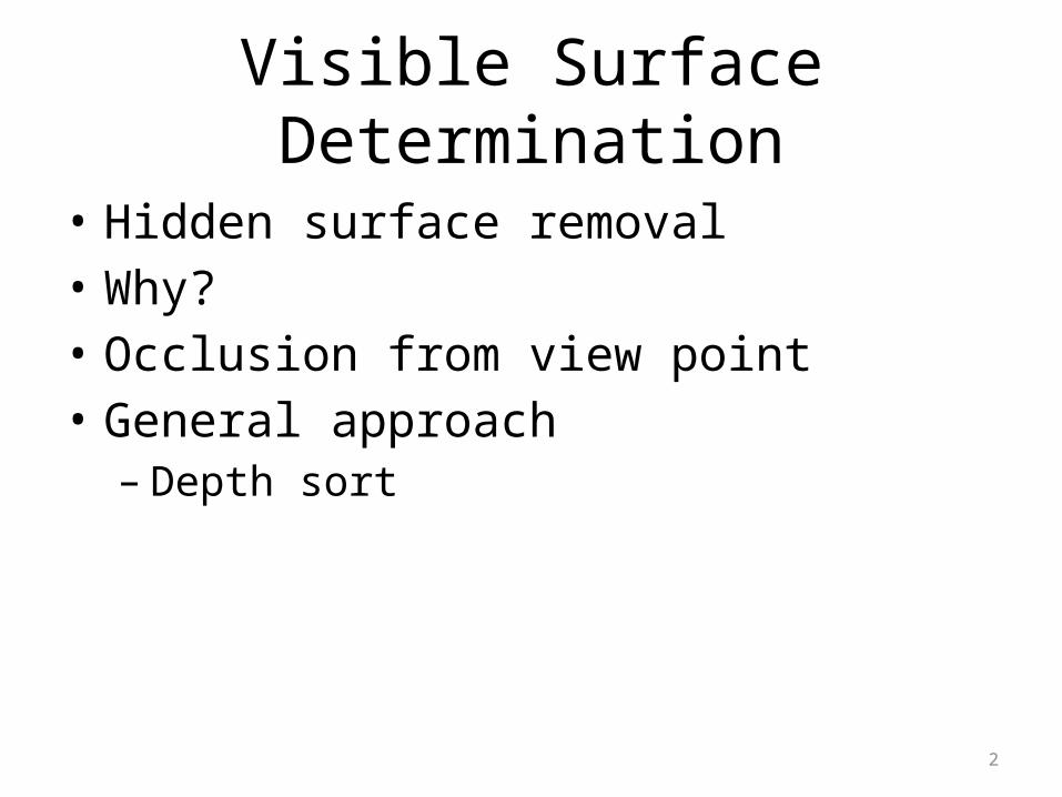
Visible Surface Determination
• Hidden surface removal• Why?• Occlusion from view point• General approach– Depth sort
3
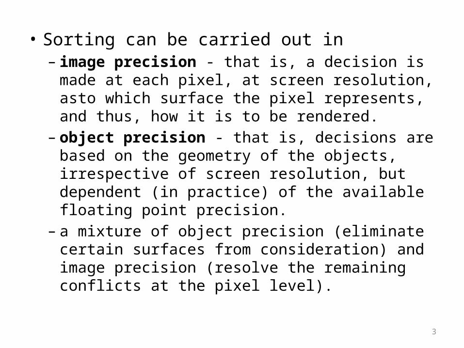
• Sorting can be carried out in – image precision - that is, a decision is made at
each pixel, at screen resolution, asto which surface the pixel represents, and thus, how it is to be rendered.
– object precision - that is, decisions are based on the geometry of the objects, irrespective of screen resolution, but dependent (in practice) of the available floating point precision.
– a mixture of object precision (eliminate certain surfaces from consideration) and image precision (resolve the remaining conflicts at the pixel level).
4
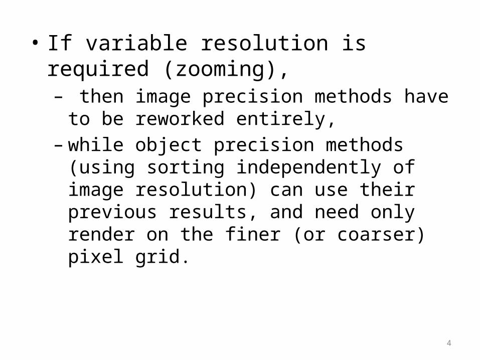
• If variable resolution is required (zooming),– then image precision methods have to be
reworked entirely, – while object precision methods (using sorting
independently of image resolution) can use their previous results, and need only render on the finer (or coarser) pixel grid.
5
• Complexity– If a scene has n surfaces, we might expect an object
precision algorithm to take O(n2) time, since every surfaces may have to be tested against every other surface for visibility.
– On the other hand, if the are N pixels, we might expect an image precision algorithm to take O(nN) time, since every pixel may have to be tested for the visibility in n surfaces.
– Since the number of pixels N usually greatly exceeds the number of surfaces, the number of decisions to be made is much fewer in the object precision case.
6
• Complexity continued– Different algorithms try to reduce these basic
counts. – Thus, one can consider bounding volumes (or
“extents”) to determine roughly whether objects cannot overlap – this reduces the sorting time.
– With a good sorting algorithm, O(n2) may be reducible to a more manageable O(n log n).
– Concepts such as depth coherence (the depth of a point on a surface may be predicable from the depth known at a nearby point) can cut down the number of arithmetic steps to be performed.
7
z-Buffer approach
• Image precision algorithms may benefit from hardware acceleration.
• The z-buffer algorithm requires a depth buffer (z-buffer) d[x][y] to record the nearest the rendering of the nearest point encountered so far, to by placed at pixel (x,y).
• The algorithm relies on the fact that if a nearer object occupying (x,y) is found, then the depth buffer is overwritten with the rendering information from this nearer surface.
8
z-Buffer algorithm
• Image precision algorithms may benefit from hardware acceleration.
• The z-buffer algorithm requires a depth buffer (z-buffer) d[x][y] to record the nearest the rendering of the nearest point encountered so far, to by placed at pixel (x,y).
• The algorithm relies on the fact that if a nearer object occupying (x,y) is found, then the depth buffer is overwritten with the rendering information from this nearer surface.
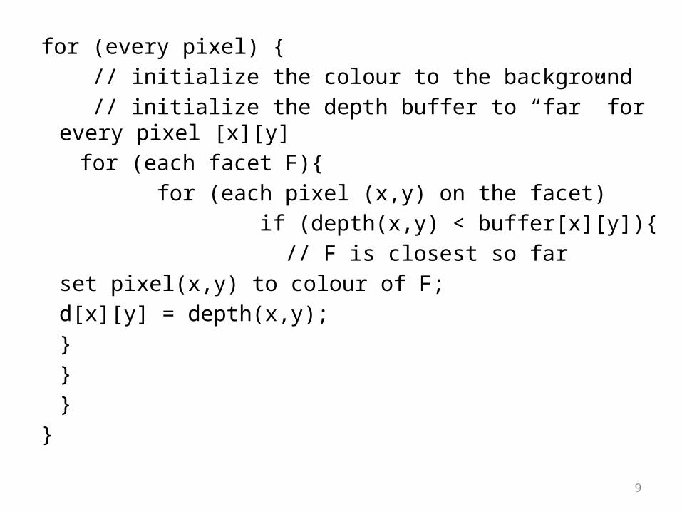
9
for (every pixel) { // initialize the colour to the background // initialize the depth buffer to “far” for every pixel [x][y] for (each facet F){ for (each pixel (x,y) on the facet) if (depth(x,y) < buffer[x][y]){ // F is closest so far
set pixel(x,y) to colour of F; d[x][y] = depth(x,y);}
}}
}
10
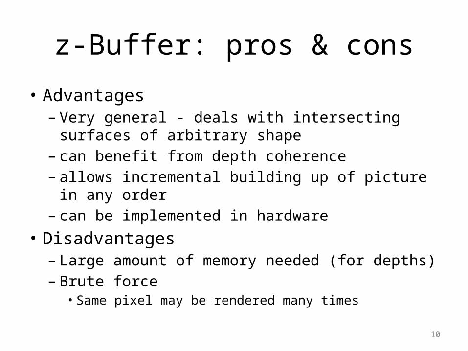
z-Buffer: pros & cons
• Advantages– Very general - deals with intersecting surfaces of
arbitrary shape – can benefit from depth coherence – allows incremental building up of picture in any order – can be implemented in hardware
• Disadvantages– Large amount of memory needed (for depths)– Brute force
• Same pixel may be rendered many times
11
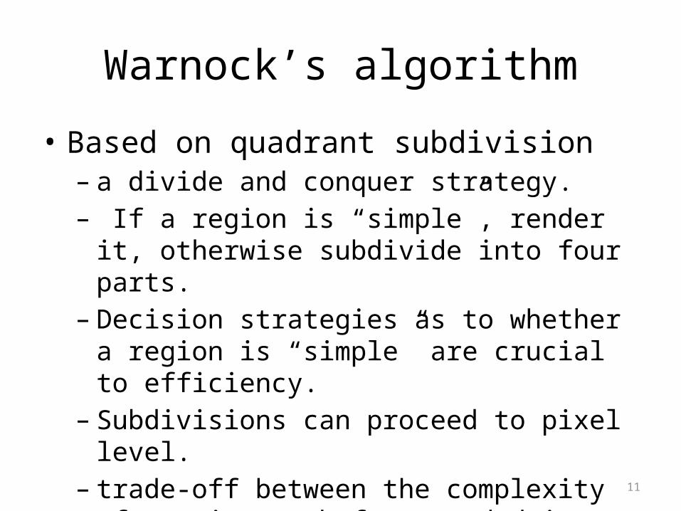
Warnock’s algorithm
• Based on quadrant subdivision – a divide and conquer strategy.– If a region is “simple”, render it, otherwise
subdivide into four parts. – Decision strategies as to whether a region is
“simple” are crucial to efficiency. – Subdivisions can proceed to pixel level.– trade-off between the complexity of testing each
facet and doing further subdivision.
12
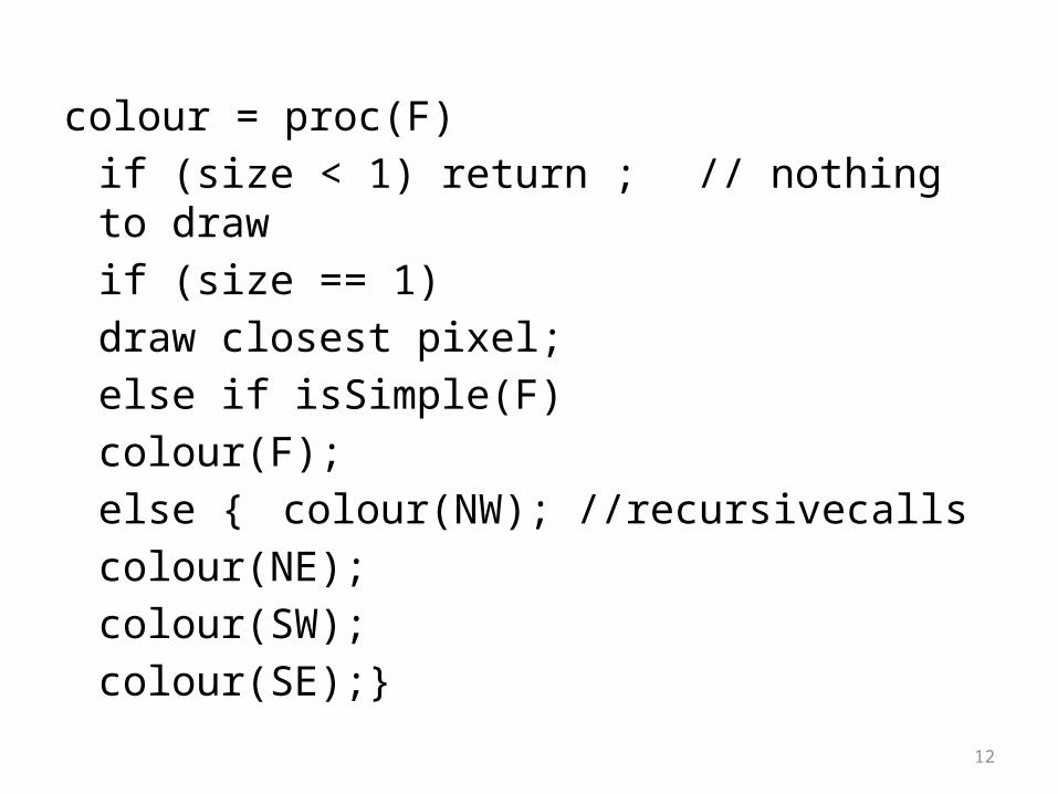
colour = proc(F)if (size < 1) return ; // nothing to draw if (size == 1)
draw closest pixel; else if isSimple(F)
colour(F); else {colour(NW); //recursivecalls
colour(NE);colour(SW); colour(SE);}

13
Warnock’s alg.: pros & cons
Of historical interest!• Advantage– Simple to implement
• Disadvantages– Enforces a seemingly haphazard rendering order
(unimportant if results are assembled in a buffer)– Scanline coherence difficult to apply– Subdivisions may be forced to pixel level
14
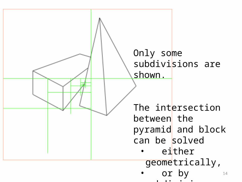
Only some subdivisions are shown.
The intersection between the pyramid and block can be solved • either geometrically, • or by subdivision
until a solution becomes feasible.
15
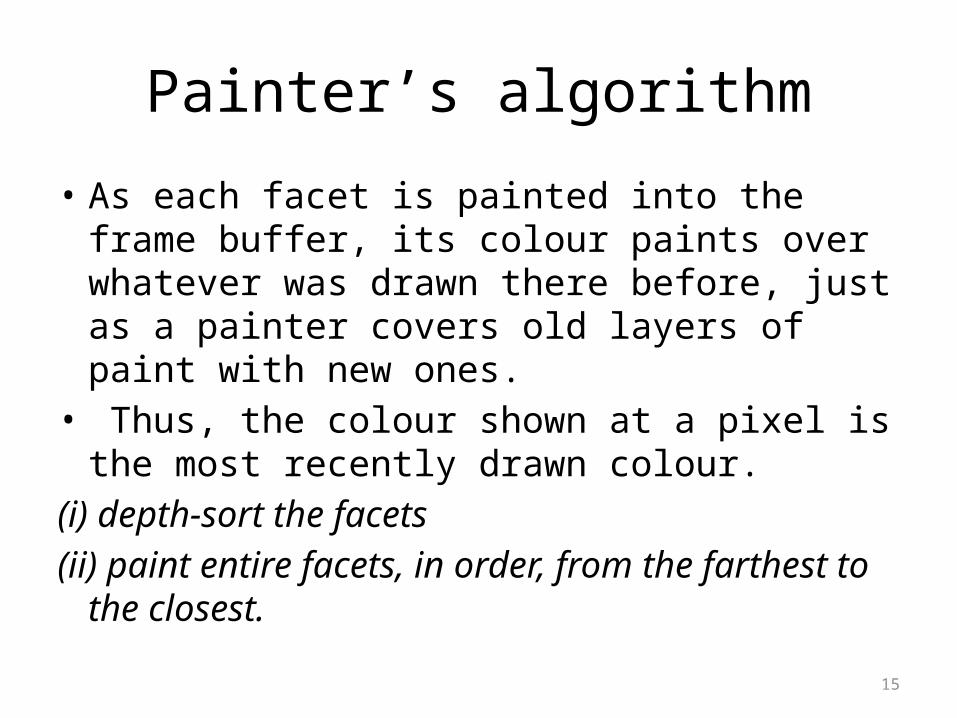
Painter’s algorithm
• As each facet is painted into the frame buffer, its colour paints over whatever was drawn there before, just as a painter covers old layers of paint with new ones.
• Thus, the colour shown at a pixel is the most recently drawn colour.
(i) depth-sort the facets(ii) paint entire facets, in order, from the farthest
to the closest.
16
Painter’s algorithm
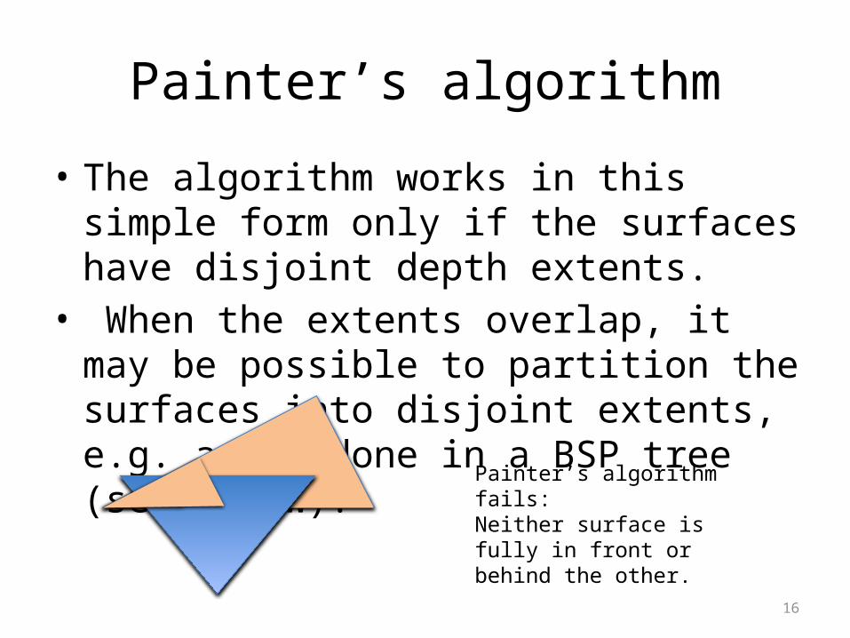
• The algorithm works in this simple form only if the surfaces have disjoint depth extents.
• When the extents overlap, it may be possible to partition the surfaces into disjoint extents, e.g. as is done in a BSP tree (see below).
Painter’s algorithm fails:Neither surface is fully in front or behind the other.
17
BSP trees – binary space partition
• Binary tree sort• Recursive• Build the tree– Insert nodes, in some order, in the left or right sub-
tree, according to potential occlusion by root• Traverse tree – according to view
18
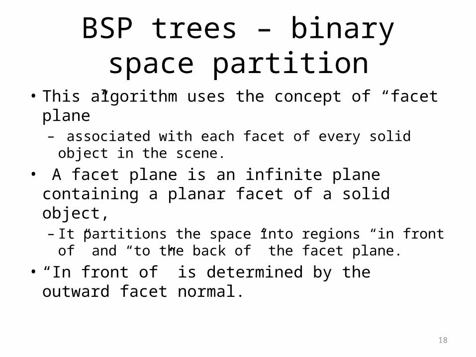
BSP trees – binary space partition
• This algorithm uses the concept of “facet plane”– associated with each facet of every solid object in
the scene.• A facet plane is an infinite plane containing a
planar facet of a solid object, – It partitions the space into regions “in front of” and
“to the back of” the facet plane.• “In front of” is determined by the outward facet
normal.
19
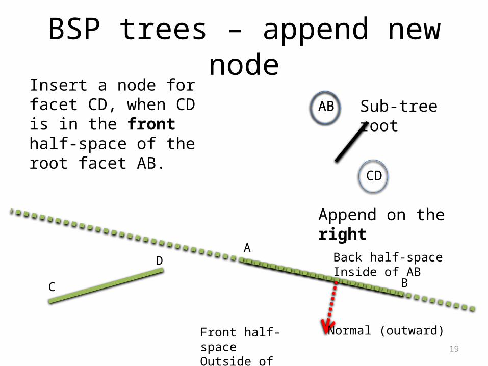
BSP trees – append new node
A
B
Normal (outward)
C
D
Append on the right
ABAB
CD
Insert a node for facet CD, when CD is in the front half-space of the root facet AB.
Sub-tree root
Back half-spaceInside of AB
Front half-spaceOutside of AB
20
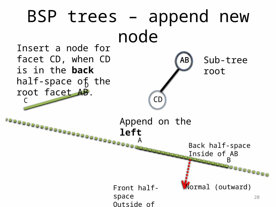
A
B
Normal (outward)
C
D
AB
CD
Append on the left
ABABInsert a node for facet CD, when CD is in the back half-space of the root facet AB.
Sub-tree root
BSP trees – append new node
Back half-spaceInside of AB
Front half-spaceOutside of AB
21
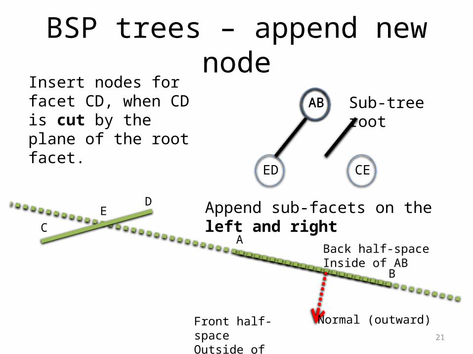
A
B
Normal (outward)
C
D
AB
ED
Append sub-facets on the left and right
ABABInsert nodes for facet CD, when CD is cut by the plane of the root facet.
Sub-tree root
BSP trees – append new node
E
CE
Back half-spaceInside of AB
Front half-spaceOutside of AB
22
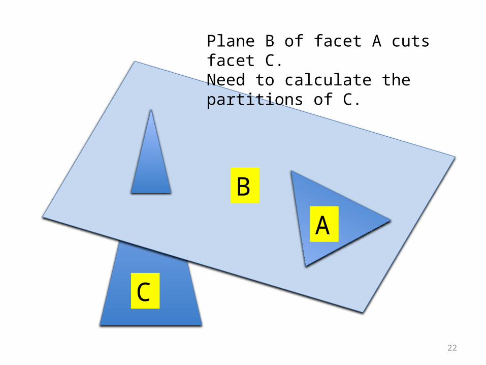
AB
C
Plane B of facet A cuts facet C.Need to calculate the partitions of C.
23
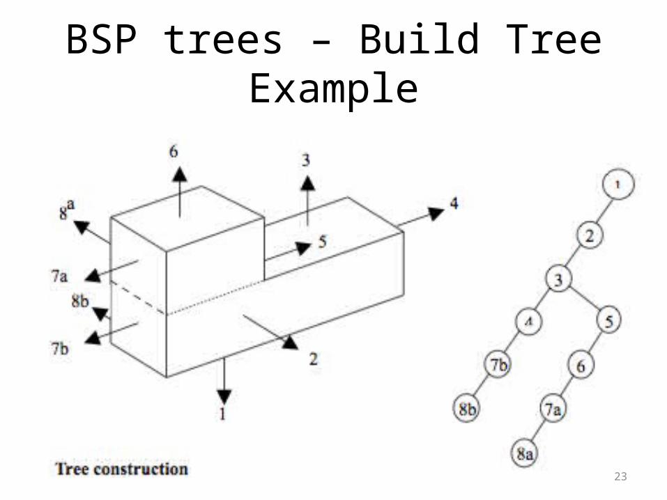
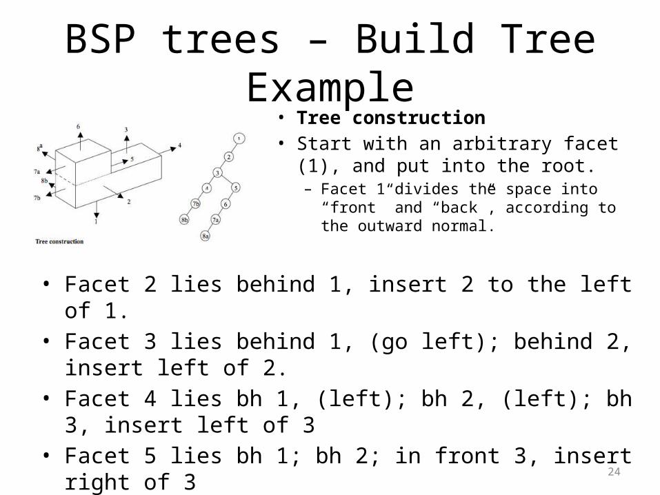
BSP trees – Build Tree Example
24
BSP trees – Build Tree Example
• Facet 2 lies behind 1, insert 2 to the left of 1.• Facet 3 lies behind 1, (go left); behind 2, insert left of 2.• Facet 4 lies bh 1, (left); bh 2, (left); bh 3, insert left of 3• Facet 5 lies bh 1; bh 2; in front 3, insert right of 3• Facet 6 lies bh 1; bh 2; in fr 3; bh 5, insert left of 5
• Tree construction• Start with an arbitrary facet (1), and
put into the root. – Facet 1 divides the space into “front” and
“back”, according to the outward normal.
25
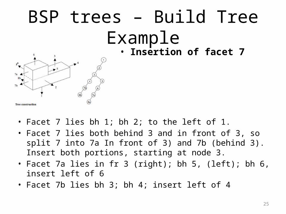
BSP trees – Build Tree Example
• Facet 7 lies bh 1; bh 2; to the left of 1.• Facet 7 lies both behind 3 and in front of 3, so split 7 into 7a In
front of 3) and 7b (behind 3). Insert both portions, starting at node 3.
• Facet 7a lies in fr 3 (right); bh 5, (left); bh 6, insert left of 6• Facet 7b lies bh 3; bh 4; insert left of 4
• Insertion of facet 7
26
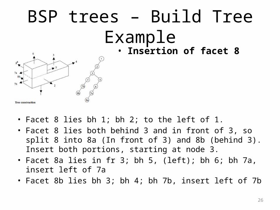
BSP trees – Build Tree Example
• Facet 8 lies bh 1; bh 2; to the left of 1.• Facet 8 lies both behind 3 and in front of 3, so split 8 into 8a (In
front of 3) and 8b (behind 3). Insert both portions, starting at node 3.
• Facet 8a lies in fr 3; bh 5, (left); bh 6; bh 7a, insert left of 7a• Facet 8b lies bh 3; bh 4; bh 7b, insert left of 7b
• Insertion of facet 8
27
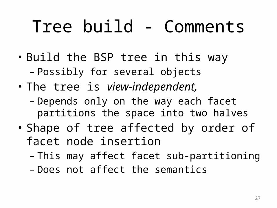
Tree build - Comments
• Build the BSP tree in this way– Possibly for several objects
• The tree is view-independent, – Depends only on the way each facet partitions the
space into two halves• Shape of tree affected by order of facet node
insertion– This may affect facet sub-partitioning– Does not affect the semantics
28
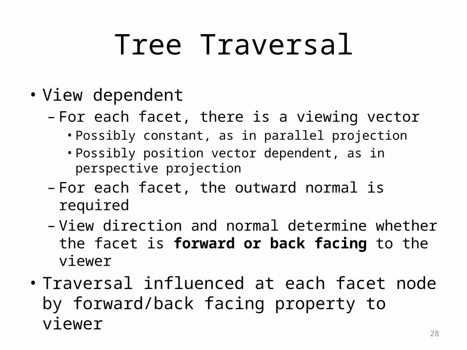
Tree Traversal
• View dependent– For each facet, there is a viewing vector• Possibly constant, as in parallel projection• Possibly position vector dependent, as in perspective
projection
– For each facet, the outward normal is required– View direction and normal determine whether the
facet is forward or back facing to the viewer• Traversal influenced at each facet node by
forward/back facing property to viewer
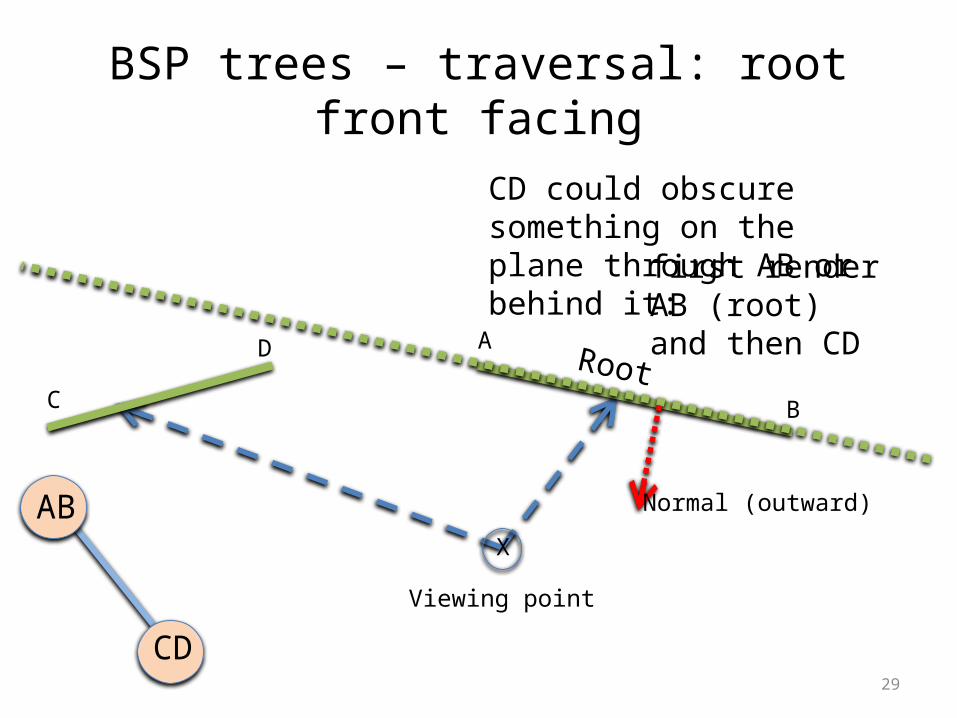
BSP trees – traversal: root front facing
29
CD could obscure something on the plane through AB or behind it:
X
A
B
Normal (outward)
Viewing point
C
D Root
first render AB (root)and then CD
AB
CD
30
E
F
BSP trees – traversal: root front facing
X
A
B
Normal (outward)
Viewing point
Root
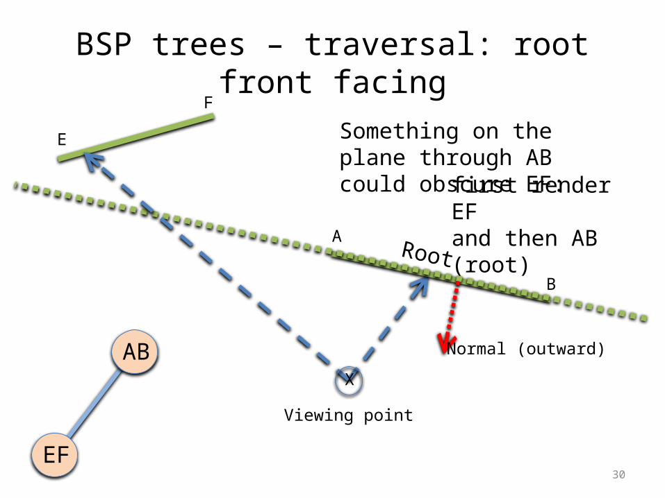
Something on the plane through AB could obscure EF:
first render EFand then AB (root)
EF
AB
31
E
F
BSP trees – traversal: root front facing
X
A
B
Normal (outward)
Viewing point
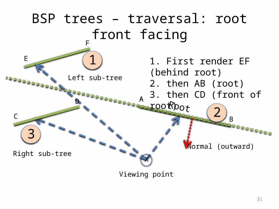
1. First render EF (behind root) 2. then AB (root)3. then CD (front of root)
RootA
C
D
1
2
3
Left sub-tree
Right sub-tree
32
BSP trees – traversal: root front facing
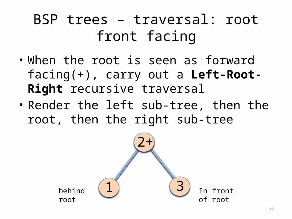
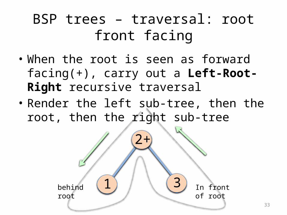
• When the root is seen as forward facing(+), carry out a Left-Root-Right recursive traversal
• Render the left sub-tree, then the root, then the right sub-tree
1
2+
3behind root
In front of root
33
BSP trees – traversal: root front facing
• When the root is seen as forward facing(+), carry out a Left-Root-Right recursive traversal
• Render the left sub-tree, then the root, then the right sub-tree
1
2+
3behind root
In front of root
34
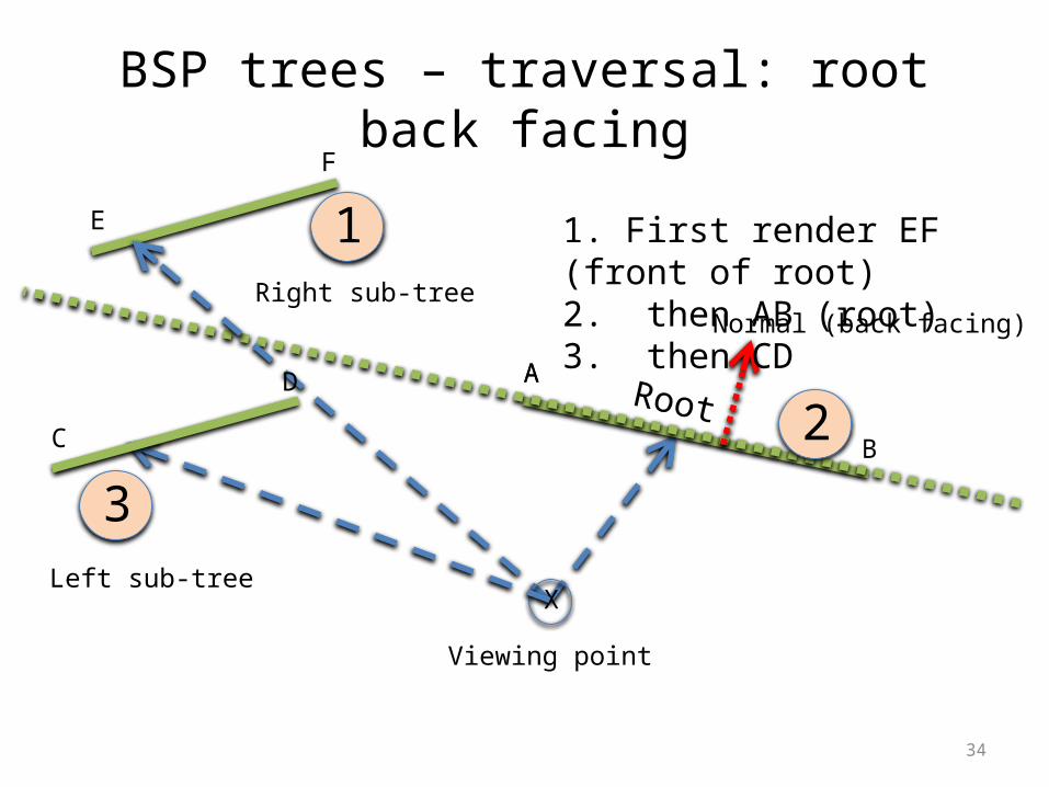
E
F
BSP trees – traversal: root back facing
X
A
B
Normal (back facing)
Viewing point
1. First render EF (front of root) 2. then AB (root)3. then CD
RootA
C
D
1
2
3
Right sub-tree
Left sub-tree
35
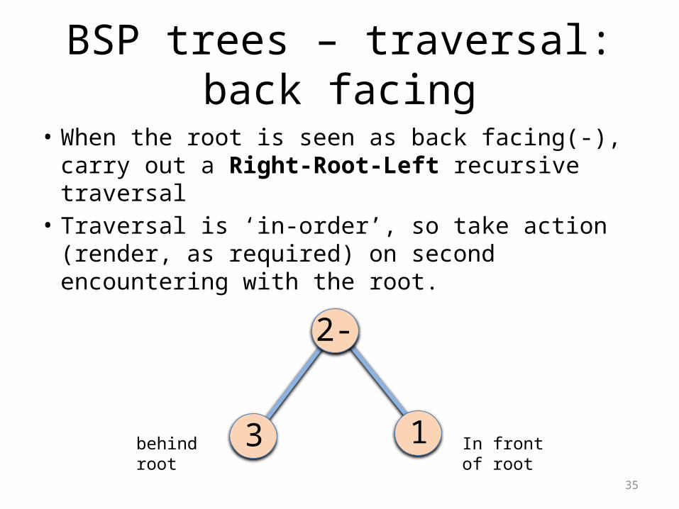
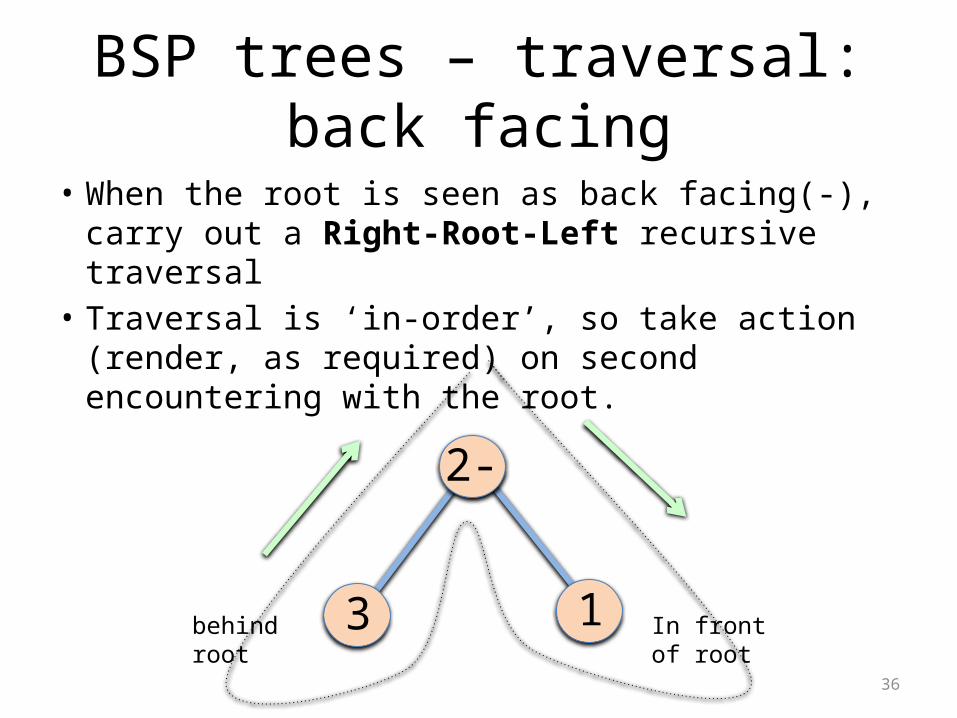
BSP trees – traversal: back facing
• When the root is seen as back facing(-), carry out a Right-Root-Left recursive traversal
• Traversal is ‘in-order’, so take action (render, as required) on second encountering with the root.
3
2-
1behind root
In front of root
36
BSP trees – traversal: back facing
• When the root is seen as back facing(-), carry out a Right-Root-Left recursive traversal
• Traversal is ‘in-order’, so take action (render, as required) on second encountering with the root.
3
2-
1behind root
In front of root
37
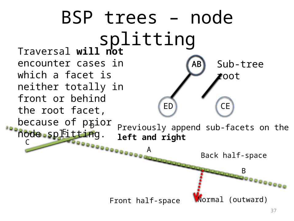
A
B
Normal (outward)
C
D
AB
ED
Previously append sub-facets on the left and right
ABABTraversal will not encounter cases in which a facet is neither totally in front or behind the root facet, because of prior node splitting.
Sub-tree root
BSP trees – node splitting
E
CE
Front half-space
Back half-space
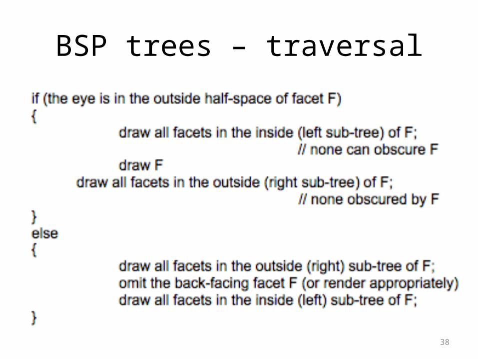
38
BSP trees – traversal
39
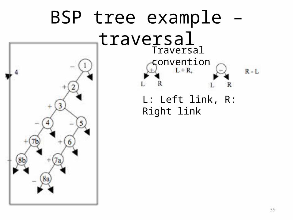
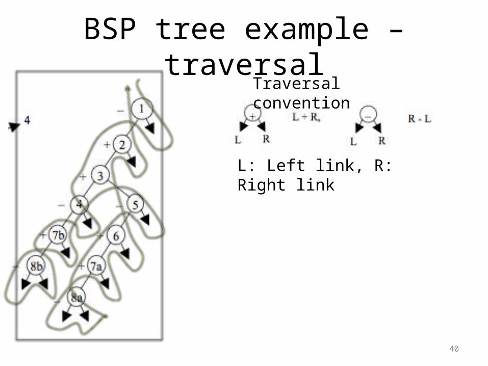
BSP tree example – traversalTraversal convention
L: Left link, R: Right link
40
BSP tree example – traversalTraversal convention
L: Left link, R: Right link
41
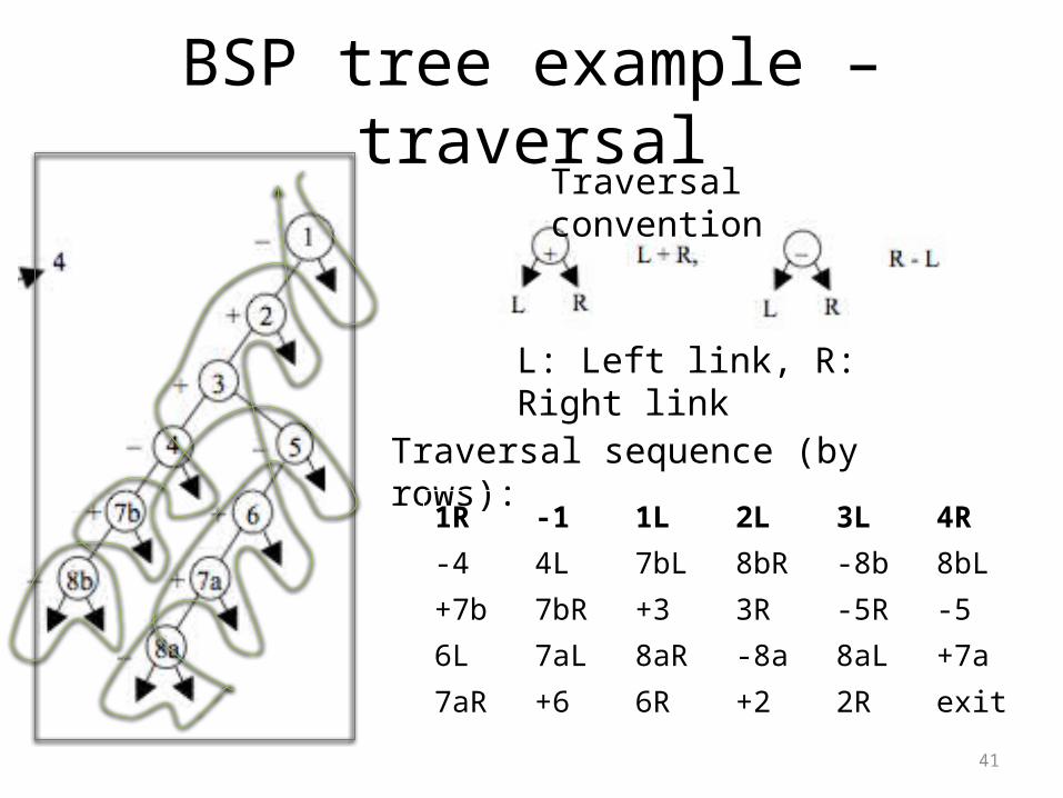
BSP tree example – traversalTraversal convention
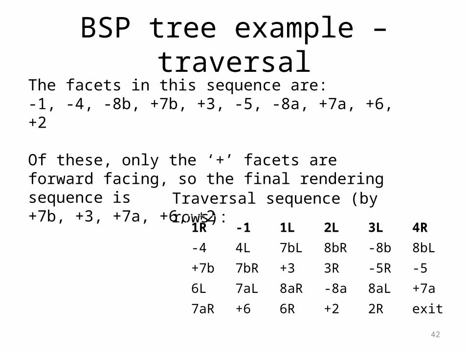
Traversal sequence (by rows): 1R -1 1L 2L 3L 4R
-4 4L 7bL 8bR -8b 8bL
+7b 7bR +3 3R -5R -5
6L 7aL 8aR -8a 8aL +7a
7aR +6 6R +2 2R exit
L: Left link, R: Right link
42
BSP tree example – traversal
Traversal sequence (by rows):
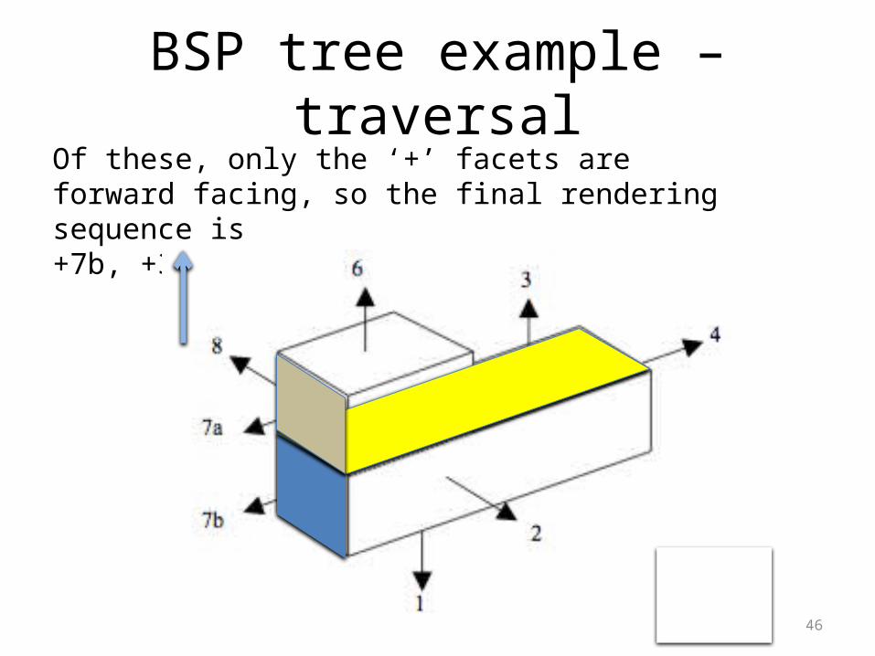
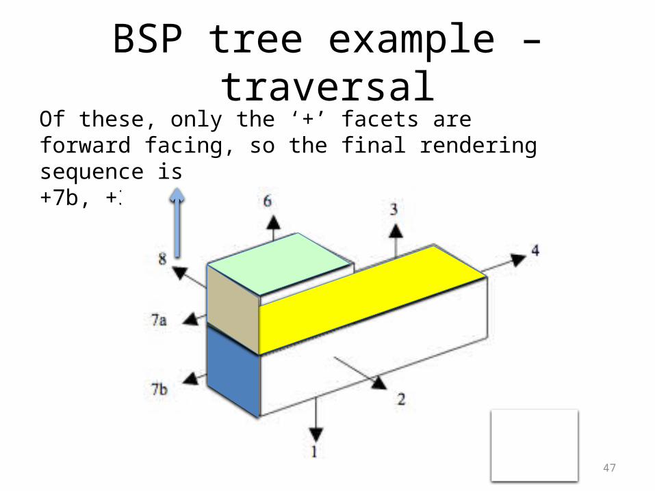
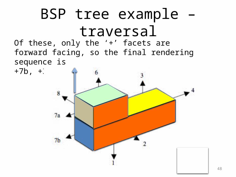
The facets in this sequence are:-1, -4, -8b, +7b, +3, -5, -8a, +7a, +6, +2
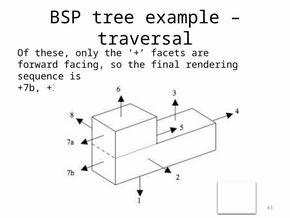
Of these, only the ‘+’ facets are forward facing, so the final rendering sequence is+7b, +3, +7a, +6, +2
1R -1 1L 2L 3L 4R
-4 4L 7bL 8bR -8b 8bL
+7b 7bR +3 3R -5R -5
6L 7aL 8aR -8a 8aL +7a
7aR +6 6R +2 2R exit
43
BSP tree example – traversalOf these, only the ‘+’ facets are forward facing, so the final rendering sequence is+7b, +3, +7a, +6, +2
44
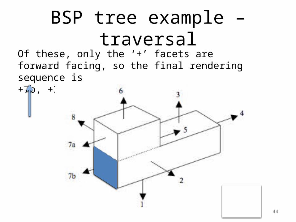
BSP tree example – traversalOf these, only the ‘+’ facets are forward facing, so the final rendering sequence is+7b, +3, +7a, +6, +2
45
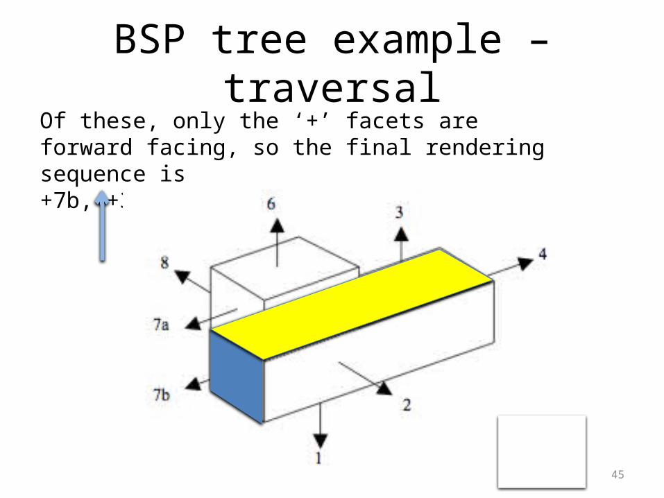
BSP tree example – traversalOf these, only the ‘+’ facets are forward facing, so the final rendering sequence is+7b, +3, +7a, +6, +2
46
BSP tree example – traversalOf these, only the ‘+’ facets are forward facing, so the final rendering sequence is+7b, +3, +7a, +6, +2
47
BSP tree example – traversalOf these, only the ‘+’ facets are forward facing, so the final rendering sequence is+7b, +3, +7a, +6, +2
48
BSP tree example – traversalOf these, only the ‘+’ facets are forward facing, so the final rendering sequence is+7b, +3, +7a, +6, +2
49
Backface culling
• This was considered in the lecture notes on projections
• Easy to apply• Object precision method – can sometimes be
used with other algorithms to reduce the facet candidates that need to be considered for visible surface determination (e.g. z-buffer).
• An integral part of the BSP-tree method.
50
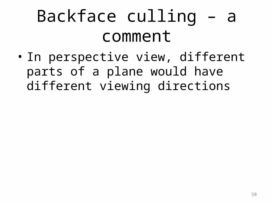
Backface culling – a comment
• In perspective view, different parts of a plane would have different viewing directions
51
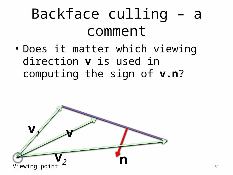
Backface culling – a comment
• Does it matter which viewing direction v is used in computing the sign of v.n?
n
v1
v2
v
X
Viewing point
52
Backface culling – a comment
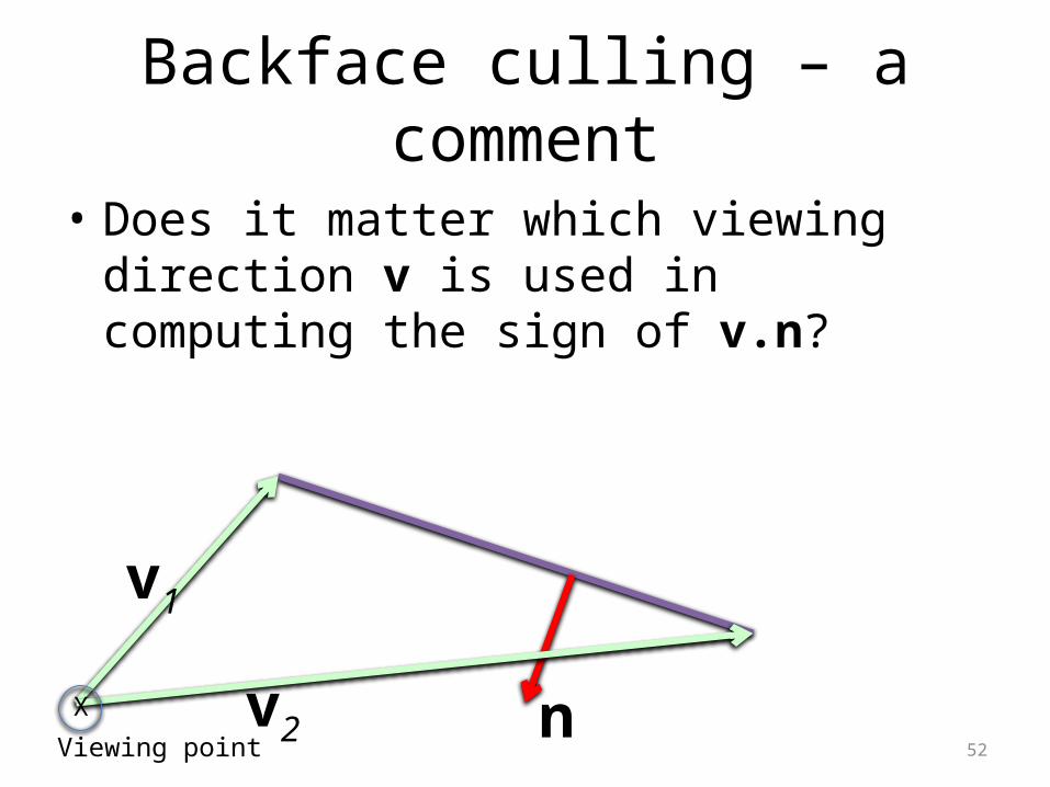
• Does it matter which viewing direction v is used in computing the sign of v.n?
n
v1
v2X
Viewing point
53
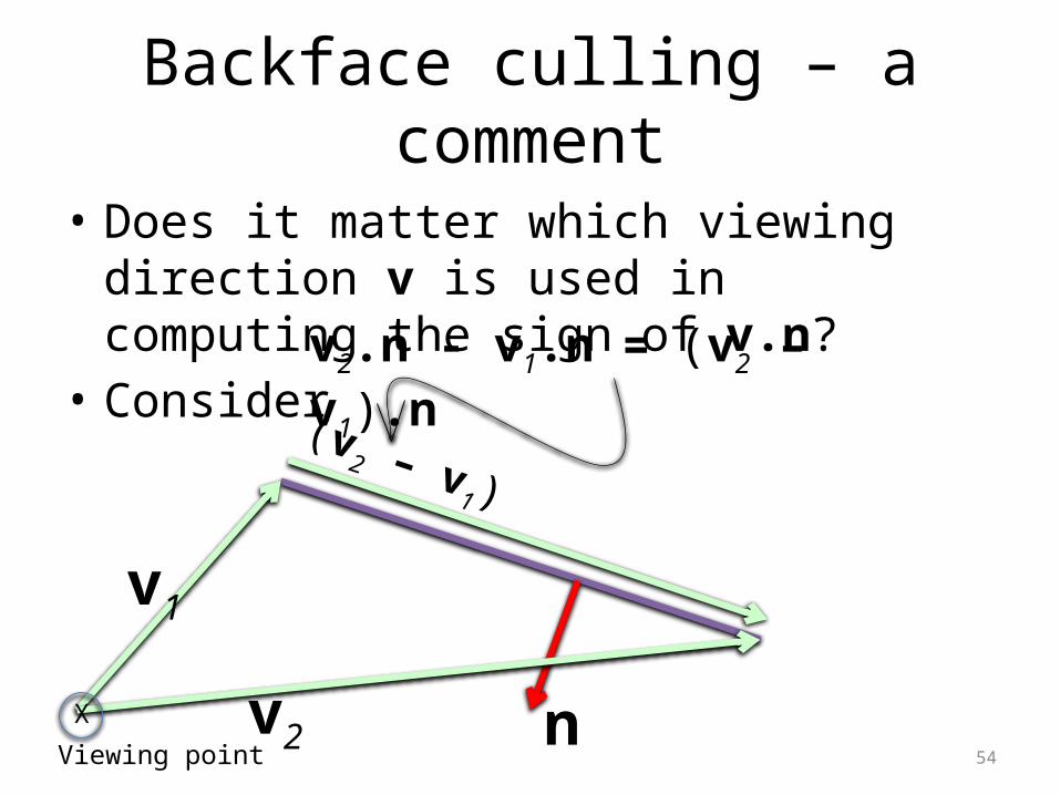
Backface culling – a comment
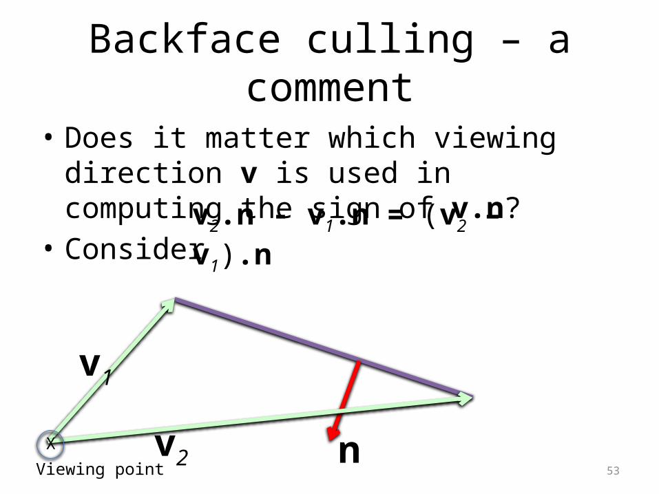
• Does it matter which viewing direction v is used in computing the sign of v.n?
• Consider
n
v1
v2
v2.n - v1.n = (v2 – v1).n
X
Viewing point
54
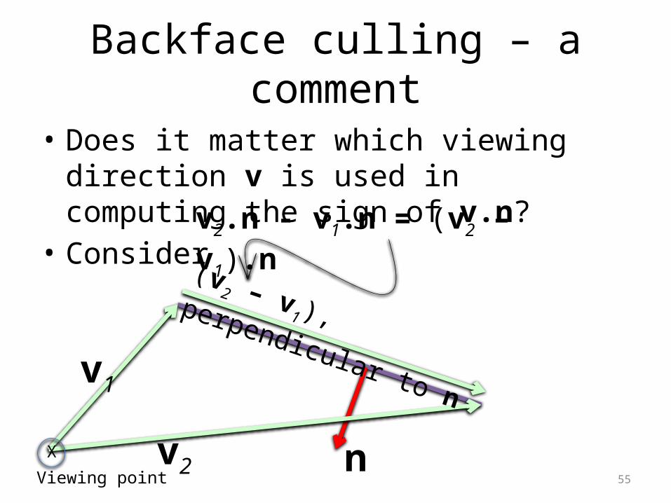
Backface culling – a comment
• Does it matter which viewing direction v is used in computing the sign of v.n?
• Consider
n
v1
v2
(v2 – v
1)
v2.n - v1.n = (v2 – v1).n
X
Viewing point
55
Backface culling – a comment
• Does it matter which viewing direction v is used in computing the sign of v.n?
• Consider
n
v1
v2
(v2 – v
1), perpendicular to n
v2.n - v1.n = (v2 – v1).n
X
Viewing point
56
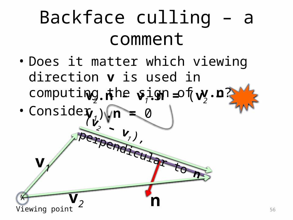
Backface culling – a comment
• Does it matter which viewing direction v is used in computing the sign of v.n?
• Consider
n
v1
v2
(v2 – v
1), perpendicular to n
v2.n - v1.n = (v2 – v1).n = 0
X
Viewing point
57
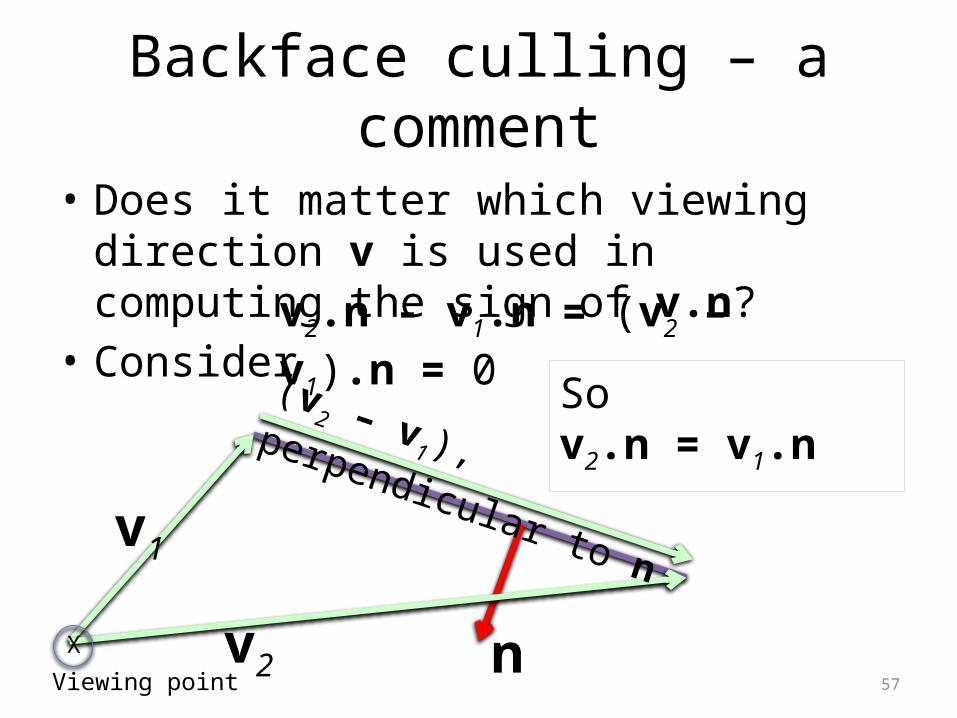
Backface culling – a comment
• Does it matter which viewing direction v is used in computing the sign of v.n?
• Consider
n
v1
v2
(v2 – v
1), perpendicular to n
v2.n - v1.n = (v2 – v1).n = 0
So v2.n = v1.nIngore this
X
Viewing point
58
Backface culling – a comment
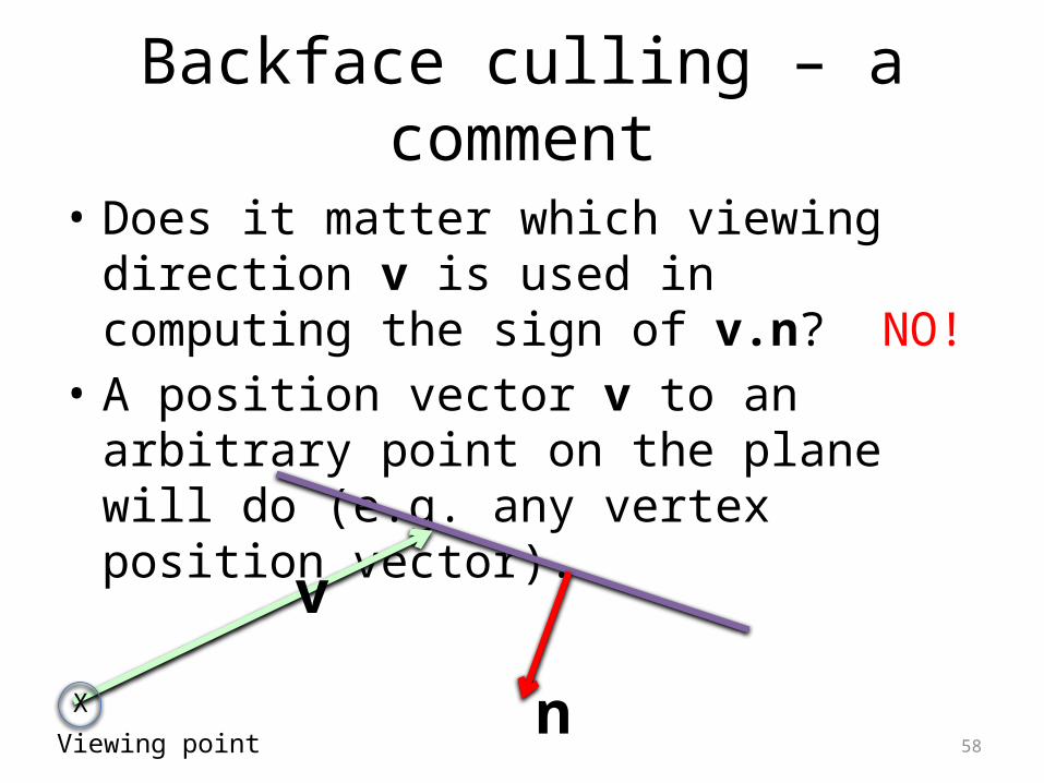
• Does it matter which viewing direction v is used in computing the sign of v.n? NO!
• A position vector v to an arbitrary point on the plane will do (e.g. any vertex position vector).
n
v
X
Viewing point

59
END