Viscous Shocks in the Destabilized Kuramoto-Sivashinsky Equation

Jens D.M. Rademacher

Weierstrass Institute for Applied Analysis and Stochastics

10117 Berlin, Germany

E-mail: rademach@wias-berlin.de

Ralf W. Wittenberg

Department of Mathematics, Simon Fraser University

Burnaby, BC V5A 1S6, Canada

E-mail: ralf@sfu.ca

March 7, 2006

We study stationary periodic solutions of the Kuramoto-Sivashinsky (KS) model for complex spa-tiotemporal dynamics in the presence of an additional linear destabilizing term. In particular, weshow the phase space origins of the previously observed stationary “viscous shocks” and relatedsolutions. These arise in a reversible four-dimensional dynamical system as perturbed heteroclinicconnections whose tails are joined through a reinjection mechanism due to the linear term. Wepresent numerical evidence that the transition to the KS limit contains a rich bifurcation structureeven within the class of stationary reversible solutions.

1

1 Introduction

Nonlinear spatially extended dynamical systems with many degrees of freedom and displayingcomplex spatial and temporal dynamics and pattern formation are ubiquitous in scientific andengineering applications [1]. The understanding of typical features of such complex and chaoticdynamics has been greatly advanced by the study of canonical models. The Kuramoto-Sivashinsky(KS) equation

ut + uxxxx + uxx + uux = 0 (1)

has been the subject of extensive study in recent decades as a prototypical example of spatiotem-poral chaos (STC) in one space dimension. Originally derived in the context of plasma instabilities[2], flame front propagation [3] and phase turbulence in reaction-diffusion systems [4], this modelhas been recognized as a generic model for long-wave primary instabilities in the presence of appro-priate symmetries [5], in particular spatial and temporal translation invariance, the odd symmetry(parity) u(x, t) → −u(−x, t), and Galilean invariance. Indeed, the role of the KS equation as amodulation equation for spatially periodic solutions in a reaction-diffusion system has been con-firmed through a recent proof [6] of closeness of corresponding solutions. On sufficiently largeL-periodic domains, the nonlinear interaction of O(L/2π) linearly unstable Fourier modes givesrise to complex dynamics of (1) in which the long-wave modes act as a “heat bath”, driving thechaotic dynamics of the most energetic modes at length scales O(2π), so that upon damping orremoval of the large-scale modes, the dynamics settles down to a regular roll solution [7, 8].

Stationary Solutions of the KS equation: The understanding of the complex dynamics andintricate bifurcation picture of (1) for varying domain sizes L begins with the (mostly unstable)stationary and travelling solutions. Since (1) with ut = 0 has a first integral (using uux =

(12u2

)x),

these may be studied as L-periodic solutions of a third-order ODE, and extensive investigationshave revealed a rich structure of odd and asymmetric solutions [9, 10, 11, 12].

In particular, the “roll” solutions (also called “cellular” states or Turing patterns) form the backboneto the KS spatial structure, and they have been studied in some detail [13]: the N -modal stateshave periodicity L/N , lie on the branch bifurcating from the trivial solution at L = N · 2π, andcan be constructed via weakly nonlinear analysis using a Fourier expansion in multiples of thefundamental wave number 2πN/L.

Of particular interest to our work on a modified KS equation are certain stationary spatiallyodd periodic solutions which consist of periodically matched so-called regular (or monotonic) andoscillatory shocks, as in Fig. 1. Such solutions, their bifurcations and relations to cells have beenstudied, for instance, in [10, 14]; they form a solitary wave train from periodically concatenatedperturbations of “solitary waves” (homoclinic orbits) such as constructed asymptotically in [15].Due to the phase space geometry of these solutions (see Fig. 1(b)), we shall refer to them as“bubbles”.

2

0.000.10

0.200.30

0.400.50

0.600.70

0.800.90

1.00

-1.5

-1.0

-0.5

0.0

0.5

1.0

1.5

0 64 128

x

u

0.5-0.5

0.61

-0.64

u

xu

(a) (b)

Figure 1: a) An odd “bubble” solution for the KS equation (α = 0) with period L = 128; b) the(u, ux) projection of another bubble solution with more oscillations.

The dKS Equation: We consider the destabilized Kuramoto-Sivashinsky (dKS) equation [16]

ut + uxxxx + βuxx + uux = αu, (2)

restricting ourselves to the (invariant) subspace of zero-mean solutions. For α = 0 and β 6= 0,equation (2) is (a rescaling of) the Kuramoto-Sivashinsky equation (1). We will typically consider(following [16]) β = 2, in which case (2) may be written in the form ut = −(1+∂2

x)2u+(α+1)u−uux;in this form, the role of the term (α+1)u in destabilizing the zero state becomes apparent. However,we retain the freedom to set the parameter β to 0, as the shock-like stationary solutions of (2) thatarise for α > 0 are robust in this limit.

The additional linear term in (2) breaks the Galilean invariance for α 6= 0, and as such (for β = 2and −1 < α < 0) has been studied in pattern formation and surface growth contexts; see [5, 16].The αu term vertically shifts the linear dispersion relation

λ = −k4 + βk2 + α (3)

for perturbations from the trivial state, and thus effectively damps (for α < 0) or drives (for α > 0)the long-wave modes. The effect on the dynamics is thus as for numerical experiments in which thelarge-scale modes in KS were suppressed or driven excessively [7, 8]: For sufficiently small α+1 > 0,the STC decays and the dynamics settle down to the regular roll state, while for α > 0 sufficientlylarge, solutions display rapidly traveling structures and shock-like features. The understanding ofSTC in the KS equation is thus advanced by studying the transition α → 0, which for α < 0 occursvia “spatiotemporal intermittency” [17].

Viscous Shocks: Motivated by the observation in [16] that for sufficiently large α, attractingshock-like odd solutions such as that in Fig. 2 have been observed in L-periodic simulations of thePDE (2), in the present work we concentrate on certain stationary solutions for α > 0, which satisfy

uxxxx + βuxx + uux = αu. (4)

3

0.000.10

0.200.30

0.400.50

0.600.70

0.800.90

1.00

-20.

-15.

-10.

-5.

0.

5.

10.

15.

20.

0 30 60

u

x

Figure 2: Odd viscous shock of period L = 60 for α = 0.4.

The “tails” of these solutions are close to spatially linear solutions with slope α: indeed (4) has theexact solution u(x) = αx. The shock-like interface arises when u is constrained to be periodic, andwe shall see below that as L → ∞, the interface scales to a jump for L−1u(Lx); thus we refer tothese solutions as viscous shocks.

The origin of viscous shocks as L-periodic orbits in the four-dimensional phase space associatedwith (4) is discussed at some depth in §4: The emergence of viscous shocks is due to a reinjectionmechanism for α > 0 by which certain heteroclinic solutions become periodic. Precisely the sameeffect, but in a much simpler context, occurs in the so-called Burgers-Sivashinsky equation [18],and for illustrative purposes we discuss it in some detail in §3.

In the limit of unbounded period, viscous shocks exist up to α = 0 and converge to fronts in theKS equation. As the integration constant for the stationary KS equation becomes unbounded,the aforementioned bubbles converge to the same fronts [9, 10]. It might thus seem natural thatviscous shocks bifurcate from bubbles as α increases from 0. In §5 we present numerical evidencethat viscous shocks for large α are indeed path-connected to bubbles in the (α, L)-parameter space.However, it appears that for fixed period L, there is no connection in α from α = 0 to viscousshocks for large α; instead, as α decreases viscous shocks either destabilize in a Hopf bifurcation orcease to exist at a fold point at some α > 0.

Viscous Shocks as a Source-Sink Compound: For the PDE (2), one may heuristically viewviscous shocks as a robust connection between a “source” at the center (zero-intercept) of the tailand a “sink” at the shock interface, because localized perturbations between the two zero-interceptsare transported towards the shock interface, as indicated by the cartoon in Fig. 3(a). Indeed, thevariation w = u−αx about the linear part in the profile (choosing x = 0 at the center of the lineartail) satisfies

wt + αxwx = −(wxxxx + βwxx + wwx).

For small, smooth initial w(·, 0) localized near any x 6= 0 we expect that the right-hand side ofthe above equation remains much smaller than αxwx due to smoothness, at least for a short time.Neglecting the right-hand side during this time, for α > 0 the coefficient αx of the convection

4

0.000.10

0.200.30

0.400.50

0.600.70

0.800.90

1.00

-20.

-15.

-10.

-5.

0.

5.

10.

15.

20.

u

x0 30 60

0 10 20 30 40 50 60

0

2

4

6

8

10

12

14

−40

−20

0

20

40

t

x

(a) (b)

Figure 3: (a) Schematic depiction of direction of transport of localized perturbations along the tailof a viscous shock. (b) Time evolution of the dKS equation for L = 60, α = 0.5; initial condition isa viscous shock with a small Gaussian perturbation near x = 4. Note the accelerated transport nearthe interface.

term is positive for positive x, implying transport away from a “source” at x = 0 where u = 0,ux ≈ α, to the right for positive x and to the left for negative x. Since the transport depends onthe u-elevation, one may interpret it as a remnant of the Galileian invariance of the KS equation(α = 0). In fact, the characteristics of the hyperbolic part on the left hand side are (t, x0 eαt), whichimplies a spreading of the perturbations from the center and an accelerated transport towards theshock interface.

This effect is observed in numerical simulations of the dKS equation (2), such as that plotted inFig. 3(b), in which the (stable) viscous shock for L = 60, α = 0.5 initially receives a small Gaussianperturbation along the tail to the right of u = 0. Note the direction of transport of perturbationsof the linear tail, to the right for u > 0 and to the left for u < 0, and the distinct accelerationnearing the interface as predicted; the final stationary state is a translation of the original viscousshock. For smaller α, for which the viscous shock is no longer an attractor, similar persistent wavetransport towards the (remnants of the) interface is characteristic of the transition to STC as α

decreases to 0.

Scaling of Bounds on the Attractor: The existence of large amplitude viscous shock solutionsis of particular interest in the context of the scaling of rigorous bounds on the dKS attractor (see[16, 19] for discussions). All numerically computed or analytically approximated known solutionsof the KS equation (1) on bounded domains of length L appear to have amplitude |u(x, t)| uni-formly bounded independent of L; but while partial proofs of this are known, notably the resultof Michelson [9] of a uniform bound for all stationary solutions, a general L∞ bound for (1) hasremained elusive. Analytical estimates typically proceed via the L2 norm, defined by the energy‖u‖2

2 =∫ L0 u2 dx; uniform boundedness of u would imply lim supt→∞ ‖u‖2 ≤ CL1/2, or that the

energy density is finite. This scaling appears natural in the spatiotemporally chaotic KS limit, as itis consistent with decay of spatial correlations and extensivity, that is, local dynamics independent

5

of system size and unaffected by distant boundaries.

The asymptotic scaling of the viscous shock solutions of (2), as observed numerically [16] andshown in §4 below, shows that the dKS equation does not have extensive dynamics: For anyα > 0, as the period L → ∞ the L∞ and L2 norms scale as ‖u‖∞ = O(αL), ‖u‖2 = O(αL3/2),which implies that the best possible bound on the KS absorbing ball using a method valid also forα > 0 should be lim supt→∞ ‖u‖2 ≤ CL3/2. By an improved construction of the gauge functionφ, Bronski and Gambill [19] have recently shown that the exponent 3/2 can indeed be achievedusing a Lyapunov-type argument to proving bounds, and is optimal for such an approach. Thus forthe dKS equation we have the bound lim supt→∞ ‖u‖2 ≤ C(α)L3/2, and the viscous shock solutionsaturates the bound. (The best current estimate for the absorbing ball of the KS equation for α = 0is lim supt→∞ ‖u‖2 = o(L3/2), using a method, inapplicable for α > 0, of treating the KS solutionat large scales like an entropy solution of Burgers’ equation [20]).

2 Phase space formulation for stationary solutions

In preparation for studying the stationary solutions of the dKS equation, we rewrite equation (4)as a first order system:

ux = u1

u1,x = u2

u2,x = u3

u3,x = −βu2 − uu1 + αu

(5)

or, more briefly, Ux = F (U ;α), where we denote U = (U0, U1, U2, U3) = (u, u1, u2, u3). Thesystem (5) is measure-preserving, because the trace of its linearization vanishes. The odd symmetryu → −u, x → −x of (4) yields the reversible symmetry of (5) with respect to the reflectionR(u, u1, u2, u3) = (−u, u1,−u2, u3), which has the symmetry plane SR = {(0, a, 0, b)|a, b ∈ R},orthogonal to the flow. We refer to solutions that are symmetric with respect to the reflection asreversible.

The single odd linear solution αx of (4) plays an important role, and we view it as an invariantreversible one-dimensional manifold `α = {(a, α, 0, 0)|a ∈ R} in the phase space of (5); note that `0

is a line of equilibria.

In anticipation of the stability considerations in §5, we introduce the linearization of (2) about asolution u(x),

L(u)v = vxxxx + βvxx + vux + uvx − αv. (6)

The eigenvalue problem λv+L(u)v = 0 with appropriate boundary conditions (possibly at infinity)determines the spectrum of L(u) (also referred to as the spectrum of u) for the PDE (2) and therebythe stability of a stationary solution u. We recast this eigenvalue problem as a first-order linear

6

non-autonomous ODE of the form Vx = B(x;λ)V , where B(x;λ) = A(u(x), ux(x), λ) with

A(u, u1, λ) := ∂UF (U ;α)− λ

0 0 0 00 0 0 00 0 0 01 0 0 0

=

0 1 0 00 0 1 00 0 0 1

α− u1 − λ −u −β 0

. (7)

Note that for λ = 0 this is the linearization of the spatial dynamics (5) in u.

For α 6= 0 the unique spatially uniform steady state u(x) = 0 of (2) corresponds to the uniqueequilibrium U = (0, 0, 0, 0) in (5). The eigenvalues of the linearization A(0, 0, 0) about the trivialstate are

±ν±(α) = ±

√−β

2±

√β2

4+ α,

whose real and imaginary parts are monotone functions of α. In particular, ν−(0) =√

βi, ν+(0) = 0,and for β = 2 we have ν±(−1) = i. Hence, for β = 2, as α varies from 0 to −1 all resonances occur,which has consequences for the bifurcation of periodic orbits [10].

However, our interest is the destabilized regime α > 0, where the aforementioned viscous shocksshown in Fig. 2 were found. In this regime, A(0, 0, 0) has a pair of complex conjugate pure imag-inary eigenvalues and two non-vanishing real eigenvalues with same absolute value but oppositesigns. Hence, using Devaney’s reversible Lyapunov center theorem for reversible equilibria [21,Theorem 8.1] and the formulas for ν±(α), we can immediately deduce the existence of a familyof periodic orbits in a manifold tangent to the center eigenspace: For any α > 0 and β ≥ 0, sys-tem (5) possesses a two-dimensional invariant manifold containing the origin which consists of anested one-parameter family of reversible periodic solutions, whose period tends to 2π/|ν−(α)| asthe initial condition approaches the origin.

These symmetric periodic orbits, similar to Turing patterns, are roll (or cellular) solutions, which apriori have small amplitude, but numerically continue to solutions with relatively large amplitude;examples of such patterns (with fixed period L and varying α) are shown in Fig. 12 below. Thewavelength of these stationary patterns is set by the condition λ = 0, where the spectrum (3) of thetrivial solution u ≡ 0 crosses the imaginary axis at nonzero wave number k2 = β/2±

√β2/4 + α.

3 Burgers-Sivashinsky equation

To illustrate the phase space analysis for the investigation of steady states of (2) and for comparison,we consider the simpler destabilized Burgers or so-called “Burgers-Sivashinsky” (B-S) equation[18, 19]

ut − uxx + uux = αu. (8)

For α > 0, this equation has similar viscous shock-like solutions, consisting of an outer linearsolution and a steep inner transition layer which is near a heteroclinic connection.

7

−4 −3 −2 −1 0 1 2 3 4−4

−3

−2

−1

0

1

2

3

4

u

u 1

−4 −3 −2 −1 0 1 2 3 4−4

−3

−2

−1

0

1

2

3

4

u

u 1

−4 −3 −2 −1 0 1 2 3 4−4

−3

−2

−1

0

1

2

3

4

u

u 1

mR

(a) (b) (c)

Figure 4: Phase portraits for stationary solutions of the Burgers-Sivashinsky system (9) for (a)α = −1, (b) α = 0 and (c) α = 1.

The first order system for stationary solutions of (8) is

ux = u1

u1,x = uu1 − αu; (9)

this system is reversible with symmetry line mR = {u = 0}, and has the same linear solution u = αx

as (4), whose orbit in (9) we denote by `α as well. Since the phase space is only two dimensional,the analysis is simple, and we can give a complete characterization of stationary solutions. We firstshow that for α ≤ 0 there are no nontrivial periodic solutions, and then consider α > 0.

For α < 0, elementary phase plane analysis shows that the unique equilibrium at the origin u = 0is the only bounded stationary solution of (8) (see Fig. 4(a)). For α = 0, the line `0 = {u1 = 0}consists of fixed points which we denote by u = ±c, c ≥ 0. Orbits in the half-plane u1 > 0 areunbounded, but the region u1 < 0 is fibered by spatially heteroclinic odd orbits hc(x), as shown inFig. 4(b). These are the only nontrivial bounded stationary solutions and satisfy hx,c = 1

2(h2c − c2),

hc(∓∞) = ±c. Choosing the spatial origin so that hc(0) = 0, we find c =√−2hc,x(0), and hence

upon integration the explicit formula hc(x) = −c tanh (cx/2).

Viscous Shocks in the B-S Equation: We may summarize the behavior for α > 0 as follows:

Theorem 1 For any α > 0 the flow of (9) maps mR ∩ {u1 < 0} to mR ∩ {0 < u1 < α} re-versing the order of the u1 component. The nontrivial, bounded stationary solutions of (8) aregiven by a one-parameter family uc(x) of nested spatially periodic odd solutions, parameterized byc =

√−2uc,x(0) ∈ R+. Letting L = L(α, c) be the period of such a solution, the slope ux = u1

increases monotonically for x ∈ [0, L/2], and L → 2π/√

α as c → 0. As c → ∞, for fixed x

the solutions uc(x) converge locally uniformly to hc(x), and uc(·+ L/2) converge locally uniformlyto `α. In this limit, we can estimate the period as L = 2c/α (1 + o(1)c→∞), the amplitude asαL + o(1)c→∞ < 2 max{u(x) | x ∈ [0, L]} < αL, and uc,x(L/2) = α + O(e−c2/2α)c→∞.

8

Proof. We prove the above statements by using reversibility and phase space methods to identifythe periodic solutions, emphasizing a readily generalized geometric approach; the correspondingphase portrait for α = 1 is shown in Fig. 4(c):

For α > 0, the unique fixed point is again at the origin (u, u1) = (0, 0). The invariant line `α

and the region above it contain no bounded solutions, since for ux = u1 ≥ α, u is monotonicallyincreasing.

We parametrize the solutions Uc = U(x) = (u, u1) of (9) below `α by c ≥ 0, so that U(0) = (0,−12c2)

is the initial condition on the symmetry line mR ∩ {u1 < 0}. For small positive x, U enters thesector {u < 0, u1 < 0}. By (9) u is decreasing, and u1 increasing in this sector, so that theorbit U must intersect {u1 = 0} at u = −u∗(c, α), x = x1 (with u∗ > 0) to enter the sectorA = {u < 0, 0 < u1 < α}, remaining entirely below the invariant line `α. Since u and u1 areincreasing in A, we deduce that U must intersect the symmetry line mR for u1 > 0 at somex∗ = x∗(c, α). Since ux = u1 < α in region A, we have u(x) < −u∗ + α(x − x1) in this region, sothat the ‘time’ to traverse this region is x∗ − x1 > u∗/α. By reversibility, we conclude that U is aclosed orbit of period 2x∗ = L = L(c, α). Hence the phase plane below `α is fibered by reversibleperiodic orbits, for which more negative u1(0) = −1

2c2 are mapped to larger u(x∗) = u(L/2), thatis, closer to `α, and u1 = ux increases monotonically for x ∈ (0, L/2).

The eigenvalues of the linearization of (9) about the trivial solution (0, 0) are ±√

αi, which imme-diately implies the period in the limit c → 0+ of small-amplitude oscillations.

The large-amplitude limit of stationary solutions of long period may be studied by rescaling witha scale parameter δ > 0: setting x = δy, v = δu, the function v(y) satisfies (9) with α replacedby δ2α, and with vy(0) = −1

2(δc)2 = −12 c2. Thus for fixed vy(0) < 0, the convergence of v(y) to

the heteroclinic hc as δ → 0 is apparent. Since c = δ−1√−2vy(0), this corresponds for u(x) to the

limit c → ∞, in which u converges to the heteroclinic hc = −c tanh(cx/2). Since hc(∞) = −c, toleading order the amplitude and period are found from u∗ ∼ c and x∗ ∼ L/2 ∼ c/α, so u∗ ∼ αL/2(note that the contribution to the period from the heteroclinic is lower order, x1/x∗ = o(1)c→∞).

The behavior near `α is best analyzed by moving the spatial origin to the intersection mR∩{u1 > 0},and considering the variation about `α via w(x) = αx − u(L/2 + x), so that w(0) = 0, wx(0) =α − u1(L/2) > 0. Then (by reversibility) the repulsion rate of wx from wx(0) as x increasescorresponds to the attraction of u to `α in region A. The solution w satisfies wxx−αxwx = −wwx,which we integrate via variation of constants to

wx(x) = wx(0) eαx2/2−∫ x

0

eα(x2−s2)/2 w(s)wx(s) ds .

Hence on a linear level, neglecting the last term, the growth of wx in x, and hence the at-traction of `α ∩ {u < 0} in the transverse direction in (x − L/2), is super-exponential. Sincethe ‘time’ that u spends in A (until wx = α) is x∗ − x1 = c/α + o(1)c→∞, we find wx(0) =O

(e−α(x∗−x1)2/2

)= O

(e−c2/2α

), so the midpoint slope, at the intercept with mR ∩ {u1 > 0}, is

ux = α + O(e−c2/2α

)c→∞

.

9

2 4 6 8 10

-4

-2

2

4u

x

Figure 5: Profile of a “viscous shock” of the Burgers-Sivashinsky equation (8) with α = 1.

In this particular two-dimensional system, we may confirm the above conclusions directly from thefirst integral u1 + α log |α − u1| − 1

2u2 = K, where K = −12c2 + α log α

(1 + c2

2α

)for the solution

through (0,− c2

2 ). Writing w1 = 1− u1/α this becomes w1 − log w1 + u2

2α = 1 + c2

2α − log(1 + c2

2α

).

Straightforward expansions for c2/2α � 1 show that the intercepts with mR are at w1 = 1 + c2

2α

(that is, u1 = − c2

2 ), and u1 = α(1 − w∗1) for w∗1 =(1 + c2

2α

)e−(1+c2/2α) +O((w∗1)

2); and that

the maximum value of |u| (at u1 = 0) is u∗ = maxx |u| = c(1− α

c2log c2

2α + O(c−4)). In fact, we

have w1 e−w1 =(1 + c2

2α

)e−1+(u2−c2)/2α, so for small |u|, w1 ∼ w∗1 eu2/2α. Since near x = L/2,

u ∼ α(x− L/2), we have w1 ∼ eα(x−L/2)2/2, verifying the super-exponential growth.

Remark: Many of the results about the stationary solutions of (8) are contained in [18], where theargument proceeds via matched asymptotics. The purpose here is to illustrate the approach by phasespace analysis and the role of `α in organizing the “viscous shocks” of (8) for α > 0 only.

We emphasize that these bounded solutions, which are similar to the viscous shocks in (2), do notoscillate in space. A typical such orbit for α = 1 is shown in Fig. 5. In §4 we show that the viscousshocks for the four-dimensional ODE (5) arise due to a similar phase space geometry, but oscillatenear `α.

Goodman [18] investigated stability in the B-S equation, and in particular argued that (8) in thespace of periodic mean zero solutions has a gradient structure, which excludes temporal oscillationsand chaotic behavior; and that the stable stationary solutions are those whose minimal period isthe domain length.

For the dKS equation (2), both the stability and the classification of steady states are more compli-cated, and we present numerical results for the bifurcations and spectrum of viscous shocks in §5.Indeed, the linearization of (8) in a viscous shock has a real spectrum, while some viscous shocksin (2) undergo Hopf bifurcations as α is varied.

4 Existence of viscous shocks

By comparison with the B-S equation (8), the detection of viscous shocks in the dKS equation ismore challenging due to the four-dimensional phase space of (5). However, the structural similarityis that both equations produce heteroclinic connections in a rescaled limit, and that the flow along

10

the special solution αx provides a re-injection mechanism that perturbs these heteroclinic orbitsto periodic ones. The viscous shock solutions are thus constructed as periodic orbits in (4) bypatching together a perturbed heteroclinic orbit with a trajectory near the invariant line `α.

Heteroclinic Orbits: We work in coordinates appropriate to the heteroclinic connections. Toblow up the inner layer of viscous shocks, we thus rescale (2) via x = δy and balance by u = δ−3v,which upon multiplication with δ7 yields

vyyyy + vvy = δ2(−βvyy + δ2αv). (10)

We consider (10) in its first order formulation

vy = v1

v1,y = v2

v2,y = v3

v3,y = −vv1 − δ2βv2 + δ4αv,

(11)

which has the same reversible symmetry R as (5), reflection about the symmetry plane SR, andthe invariant line in these coordinates is `δ4α = {(a, δ4α, 0, 0)|a ∈ R}.

We begin by studying the unperturbed heteroclinic orbits: For δ = 0 (10) is the integrable equation

vyyyy +12(v2)y = 0, (12)

or vyyy + 12v2 = c2/2, where c is a constant (nontrivial bounded solutions are found only for positive

integration constant). In this case, rescaling via v = cw and z = (c/2)1/3y yields

wzzz = 1− w2. (13)

Apart from the hyperbolic fixed points at w± = ±1, this equation has a unique (up to translation)bounded solution, the heteroclinic orbit h(z) [22]. This orbit lies in the transverse intersectionof the two-dimensional stable and unstable manifolds of the equilibria w− = −1 and w+ = +1,respectively, and intersects the symmetry plane w = wzz = 0 with negative slope wz. We canchoose the origin z = 0 so that h is a reversible orbit, with h(±∞) = ∓1, h(0) = hzz(0) = 0, andhz(0) < 0; and we define the amplitude of the heteroclinic orbit hmax = ‖h‖∞ = maxz∈R |h(z)| > 1.

Returning to the limiting inner equation (12), we thus obtain a one-parameter family of reversibleheteroclinic orbits hc(y) = ch

((c/2)1/3y

), which connect the equilibria ±c; note that hc,yyy(0) =

c2/2hyyy(0) = c2/2. Let Hc = (hc, hc,y, hc,yy, hc,yyy) denote the solution of the first-order systemassociated with (12). Then Hc lies in the transverse intersection of the stable and unstable manifoldsWs(−c),Wu(c) of±c [9, 22]. The unique intersection of the heteroclinic orbit Hc with the symmetryplane SR is at z = 0, with Hc(0) = (0, a(c), 0, c2/2) ∈ SR, where a(c) = (c4/2)1/3hz(0) < 0 for allc > 0; observe that a(c) → −∞ as c →∞, and that the amplitude is maxy hc(y) = chmax.

11

The Invariant Line: Having discussed the unperturbed heteroclinic orbit, we next characterizethe invariant line `δ4α in the rescaled coordinates: The invariant manifold `δ4α \ {(0, δ4α, 0, 0)}of (11) is normally hyperbolic, that is, the three-dimensional transverse linear flow near `δ4α ishyperbolic away from the symmetry plane SR. For each v < 0, the eigenspaces of the linearizationof the transverse flow are transverse to the v direction, with the transverse eigenvalues consistingof one real unstable eigenvalue and a stable complex conjugate pair of eigenvalues. Moreover, forv < 0 and any δ > 0, the unstable eigenvalue is strictly monotone increasing as v decreases, andthe real parts of the stable eigenvalues, which are the leading eigenvalues, are strictly monotonedecreasing.

We prove this by linearizing (11) about v1 = δ4α, v2 = v3 = 0 at a fixed v, to find that the linearizedmatrix A(v, v1, 0) from (7) takes the α-independent form

Aδ(v) :=

0 1 0 00 0 1 00 0 0 10 −v −βδ2 0

,

whose characteristic polynomial is ν(ν3 + v + βδ2ν). In addition to the eigenvalue ν = 0, corre-sponding to the flow along the invariant line, we have three transverse eigenvalues νj(v), j = 0, 1, 2.For βδ2 = 0, these eigenvalues are straightforwardly found as νj(v) = (−v)1/3 e2πij/3, while forβδ2 > 0, the roots of the cubic are found using Vieta’s substitution ν = w − βδ2/(3w), wherew3 = g satisfies g2 + vg −

(βδ2/3

)3 = 0; we obtain

νj(v) = e2πij/3 g13 − δ2 e−2πij/3 β

3g13

, (14)

where g ∈ R is

g = −v

2+

√v2

4+ δ6

β3

27> 0.

We observe that ν0 ∈ R, and that sgn(ν0) = −sgn(v) (since for βδ2 > 0, we compute ν0 ≥ 0 if andonly if g2 ≥

(βδ2/3

)3, which from the governing quadratic equation for g > 0 holds if and only ifv ≤ 0). The monotonicity of ν0 in v is obvious for βδ2 = 0, and otherwise follows from dg/dv < 0and dν0/dg > 0.

The remaining eigenvalues νj(v), j = 1, 2 are complex conjugate, with real part Re(νj) = −12ν0,

from which the stability and monotonicity of the complex eigenvalues follows.

Therefore `δ4α is normally hyperbolic, but not uniformly, because at SR ∩ `δ4α = (0, δ4α, 0, 0) alleigenvalues lie on the imaginary axis. Since the eigenvalues are distinct, eigenspaces are transverseto each other and the v-direction is the kernel.

Phase Space Origins of Viscous Shock: Having established the properties of the invariantline and the heteroclinic connections, as for the B-S equation (9) we can locate viscous shocks astrajectories of (11) beginning in the symmetry plane SR which track an unperturbed heteroclinic

12

orbit into the vicinity of the invariant line `δ4α, and are then transported by the flow along thisline back into the symmetry plane. However, the analysis is more subtle in this case owing to thehigher dimensionality, and as discussed below, we expect that a blow-up analysis will be requiredto make the following arguments fully rigorous.

To ensure proximity to the heteroclinic solutions of (12), the construction depends on suitable small-ness conditions on both δ4α and δ2β, which may be combined in a single perturbation parameter,for instance δ2β + δ4α. However, for the sake of clarity we consider fixed, though arbitrary, valuesα > 0 and β ≥ 0, and take δ as the perturbation parameter; we observe that all constructed tra-jectories and manifolds depend smoothly on α, β and δ. For ease of notation we do not distinguishbetween constants K > 0, which may be chosen successively smaller.

Let Φy(U) denote the flow of (11). Taking initial data U ∈ SR in the symmetry plane, we letO±(U) = {Φy(U) | y ∈ R±, |y| ≤ min{|y| > 0 | (Φy(U))0 ∈ SR}} represent the partial forward orbackward orbit under the flow before the next intersection with SR = {v = 0, v2 = 0}. Usingreversibility we identify periodic solutions, with period L in y, as orbits beginning in SR, whichagain intersect SR at y = L/2.

First we observe that there are orbits beginning in SR which closely track an unperturbed hetero-clinic orbit and are attracted arbitrarily closely to the invariant line `δ4α. Indeed, consider a compactsubinterval `c1,c2

δ4α= {(v, δ4α, 0, 0)| − c1 ≤ v ≤ −c2 < 0} of `δ4α. By our previous calculations the

interval of equilibria `c1,c20 is normally hyperbolic with combined rate κ1 = Re(ν1(−c2)) > 0, since

the real parts of the eigenvalues are monotonic in v. By Fenichel theory [23, Theorem 9.1], thestable and unstable manifolds are preserved under perturbation, so that there is a K > 0 such thatwhenever 0 < δ ≤ K, the orbit segment `c1,c2

δ4αhas locally (in y) stable and unstable manifolds Ws/u

δ

such that any orbit decays towards or diverges from `c1,c2δ4α

with rate at least κ1/2, as long as it staysin these manifolds. (In fact, as for the B-S equation we observe that for a viscous shock solution,the attraction towards `δ4α is super-exponential in y − L/2.)

We recall that for δ = 0 we have a one-parameter family of heteroclinic orbits Hc, so that thestable manifold of `c1,c2

0 transversely intersects SR with negative v1-component in a curve H, andan initial condition Hc(0) = (0, a(c), 0, c2/2) in H approaches the equilibrium at U−c,0 = (−c, 0, 0, 0)for some c > 0 in an oscillatory manner.

The stable manifold Wsδ converges locally uniformly as δ → 0 to the stable manifold of `c1,c2

0 ,and the decay in the stable fibers is exponential, while the distance of the invariant line to thev-axis is δ4α, polynomial in δ. Hence for sufficiently small K > 0, for 0 < δ ≤ K the local stablemanifold Ws

δ intersects SR in a curve Hδ, which converges uniformly to a compact subset of Has δ → 0. Let Vc,δ(0) ∈ SR be an initial condition in Hδ which approaches Hc(0) as δ → 0 forsome c, −c1 ≤ −c < −c2. Then the trajectory Vc,δ = O+(Vc,δ(0)) approaches a neighborhood ofU−c,δ = (−c, δ4α, 0, 0), and thus in particular attains a positive v1 component. The flow proceedsin the direction of increasing v, and since it maps stable fibers to stable fibers, such a trajectoryremains in the stable manifold Ws

δ , retaining a strictly positive v1 component and exponentiallyapproaching the invariant line `δ4α. By continuity (possibly for smaller K > 0) for any 0 < δ ≤ K,such an orbit crosses the section {v = 0, v1 > 0}.

13

v1 ⊂ SR

δ4α

v

−c

−c2

( c4

2)1/3hz(0)

Figure 6: Sketch of the phase space projected into the (v, v1)-plane for δ > 0; note that the v1 axislies in SR. The dashed line is the heteroclinic Hc for δ = 0.

We thus now have, for a given sufficiently small δ > 0, a one-parameter family of trajectories Vc,δ,smoothly parametrized by c, which are initially perturbations of a family of heteroclinic orbits Hc,are attracted to the vicinity of the invariant line `δ4α, and then flow in the direction of increasing v

until they cross the hyperplane {v = 0}, as indicated schematically in Fig. 6. To locate a reversibleperiodic orbit, we now make use of the additional freedom in c to obtain an intersection with thesymmetry plane SR. Let bδ(c) be the value of v2 at the intersection of Vc,δ with the hyperplane{v = 0}; then we require bδ(c) = 0 (this requirement, due to the higher dimensionality of the phasespace of (11), is part of the reason for the additional complexity not present in the two-dimensionalB-S problem).

One may argue as follows: the invariant line `δ4α lies in the plane {v2 = 0, v3 = 0}. By ourprevious computations, the transverse flow in the local stable manifold is exponentially attractedto `c1,c2

δ4α(in fact, for increasing c the trajectory Vc,δ spends longer in the stable fibration, and thus

approaches the origin in (v2, v3) more closely). Furthermore, the transverse flow is an oscillation,so that the v2-v3 projection oscillates in y, hence as a function of distance along `δ4α. Since thedistance travelled along `δ4α increases with c, we expect that bδ(c) oscillates about v2 = 0 as afunction of c; consequently for sufficiently small δ, there is a c∗ = c∗(δ, α, β) so that bδ(c∗) = 0.This gives us the desired reversible periodic orbit. By construction, this orbit is initially near anunperturbed heteroclinic, and is then exponentially attracted to the invariant line `δ4α, where v1 ≈constant; so this corresponds to a viscous shock solution, as in Fig. 7. This viscous shock Vc∗,δ(y) inthe rescaled variables (corresponding to a viscous shock Uc∗,δ(x) in the original variables) dependssmoothly on the parameters δ, α and β.

We may further verify this phase space picture by looking at the geometry of the intersection of abranch of viscous shocks, obtained by fixing c∗(δ, α, β), with the symmetry plane SR. For instance,for fixed α > 0 and β ≥ 0, decreasing δ increases the length of the flow along `δ4α, and thusincreases the period L, or L in the original variables (see the discussion on scaling below). Sincethe transverse flow in the stable manifold of `δ4α is an oscillation and contraction as a functionof distance travelled, we expect the intersection with SR to spiral in towards v1 = δ4α (that is,u1 = α), v3 = 0 with decreasing δ (or increasing L); this prediction is verified in Fig. 8(a).

Numerically, one can most easily locate viscous shocks as attracting stationary solutions of the dKSequation (2) for sufficiently large α and L; however, one can also obtain good approximations by

14

-20. -15. -10. -5. 0. 5. 10. 15. 20.

-40.

-30.

-20.

-10.

0.

10.u

u

1

-20. -15. -10. -5. 0. 5. 10. 15. 20.

-50.

-25.

0.

25.

50.u

u

2

(a) (b)

Figure 7: Phase space projections of the viscous shock from Fig. 2 onto the planes (a) (u, u1) and(b) (u, u2).

0.32 0.33 0.34 0.35 0.36 0.37

-0.005

0.000

0.005

u

u3

1

22.5-27.2

77.9

-71.4

xxu C

A

B

u

(a) (b)

Figure 8: (a) Intersections of viscous shocks with SR for fixed α ≈ 0.3435 parametrized by L ∈(40, 62). (b) Projections to the (u, uxx)-plane of trajectories of (5) with α = 0.4 and initial conditionsu = uxx = uxxx = 0, and A: ux = 0.3999999991 B: ux = 0.39999999915 C: ux = 0.3999999992.

15

a shooting method in (5) (in the original variables u(x)). In this case, it is convenient to reversethe above construction, by starting in SR near ux = α and trying to hit SR = {(u, uxx) = (0, 0)}again, since by reversibility such an intersection corresponds to a periodic solution. In Fig. 8(b)we plot the results of such a shooting approach for α = 0.4, in which we varied the initial u1 = ux

and considered the projection of the resulting orbits in the (u, u2)-plane. Observe that at theintersection with u = 0, trajectories A and C indeed lie on either side of the origin uxx = 0, whichconfirms the existence of a periodic solution (near trajectory B). Note how the presence of anunstable manifold of `α leads to extreme sensitivity to the initial ux value.

Remark: The above existence argument for the dKS viscous shocks is not rigorous in its presentform, as we only have normal hyperbolicity of the invariant line `δ4α for v 6= 0, not at the intersectionwith the symmetry plane SR. Thus we are not a priori guaranteed the desired smoothness of andrates of attraction within the stable manifold Ws

δ uniformly up to SR. (Furthermore, the presenceof a two-dimensional transverse unstable manifold Wu

δ of `c1,c2δ4α

— also not present in the B-Sequation — implies that great care is needed with continuity arguments based on perturbing theorbits constructed above.)

We expect that by a so-called blow-up analysis it is possible to rigorously prove the existence ofviscous shocks and related solutions, as well as their scaling in terms of α and L as discussed below.The blow-up approach to a non-hyperbolic equilibrium with nilpotent part is a change to sphericalcoordinates together with a desingularization that renders the non-hyperbolic equilibrium a spherewith several hyperbolic equilibria and heteroclinic connections that can be treated classically. Ithas been used successfully in low ambient dimensions for singularly perturbed problems where theslow manifold is folded at a non-hyperbolic point and transitions between opposing parts producespecial solutions; straightening such a one-dimensional fold, one obtains a line of equilibria similarto `0 (see for instance [24]).

Scaling of Viscous Shocks: The constructed viscous shock solutions Vc∗,δ(y) approach thevicinity of the invariant line near v = −c∗, and then proceed towards SR with speed v1 ∼ δ4α,which occurs along a y-interval of length ∼ c∗/δ4α. The leading-order estimate of the period in y

is thus L ∼ 2c∗/δ4α, while as δ → 0, the contribution from the flow near the heteroclinic Hc∗ is oflower order, O(1) in y.

The intersections with the symmetry plane SR occur for v1 ∼ δ4α (with, presumably, exponen-tially small corrections, as for the B-S equation) along the “linear” part of the viscous shock, andv1 ∼ a(c∗) = (c∗4/2)1/3hz(0) < 0 in the transition layer region. The amplitude of the shock ismaxy∈R |v| ∼ c∗hmax + o(1)δ→0, which is slightly greater than c∗, the overshoot being due to theheteroclinic orbit.

We hence deduce the scaling of the viscous shock solutions in the original variables, x = δy andu = δ−3v. The period L along a branch of viscous shocks (with a particular c∗) satisfies L =L(δ, α, β) = δL ∼ δ · 2c∗/δ4α. Treating the period L as a parameter (which is appropriate aswe frequently seek solutions of the PDE on a domain with a given period), and solving for δ =δ(L,α, β) ∼ (2c∗/αL)1/3, we observe that each branch of viscous shock solutions is a smooth

16

three-dimensional manifold parametrized by L, α and β.

The transition layer width due to the heteroclinic, which is O(1) in y, is O(δ) = O((αL)−1/3

)in the

original x-variable, as predicted and observed numerically in [16] and used for the gauge functionconstruction in [19]. Further, since u1 = ux = δ−4vy, the intersections with the symmetry planeSR occur with slope ux ∼ α in the outer, linear regime (corresponding to the dominant balanceuux ∼ αu in (4)) and ux ∼ (αL/4)4/3 hz(0) in the center of the viscous shock. Lastly, the amplitudeis ‖u‖∞ ∼ hmax

2 αL, while the leading contribution to the L2 norm is due to the outer, linear part,giving ‖u‖2

2 ∼ α2L3/12, thus confirming the scaling results for ‖u‖∞ and ‖u‖2 discussed previously.

The existence criterion for these viscous shocks from our approach is (for fixed β ≥ 0) a smallnesscondition on δ. Since for δ → 0, δ = O

((αL)−1/3

), we thus have that

there exists a constant K∗ such that viscous shocks exist for αL ≥ K∗.

(The requirement that αδ4 be sufficiently small leads to an additional criterion that αL4 be largeenough, αL4 ≥ K∗, say, which becomes relevant for short-period solutions with large α.) Whilewe have only shown this criterion to be sufficient (not necessary), we thus suspect that the viscousshocks do not bifurcate from α = 0, that is, from solutions of the KS equation (1) with finite period,and this is shown numerically in §5 below.

5 Numerical continuation, stability and related solutions

For sufficiently large αL, the above argument indicates that viscous shocks exist, and indeed theyare numerically observed to be attracting [16]. Towards seeking to understand the nature of andtransitions towards spatiotemporal chaos in the KS equation (1), it is of interest to investigatewhat happens to the viscous shocks as α decreases towards the KS limit α = 0. In this limit,we know the viscous shocks cease to exist, both by our arguments in §4 and from the fact thatthe amplitude of the viscous shocks is proportional to L, while that of stationary KS solutions isuniformly bounded in L [9]; but one might surmise that they are connected in parameter space tosome interesting KS solutions. This idea is particularly attractive as the inner layers (in the limitof infinite period L) of viscous shocks in the dKS equation and of fronts in the KS equation are thesame, being the heteroclinic connections of (12) (see [9, Theorem 2.2]). It turns out, however, thatwhile viscous shocks are path-connected to the KS equation in the (α, L)-parameter plane, there isno direct path connection for fixed α or fixed L.

The full dynamics and bifurcations of the dKS equation in the α → 0 limit are complicated, andwe merely summarize here our preliminary investigations of the very restricted case of reversible,stationary solutions. We concentrate on solutions to the boundary-value problem for the system(5) (with β = 2) with boundary conditions u = u2 = 0 at x = 0, L/2, which by reversibility are L-periodic stationary solutions of the dKS equation (2). We continue these solutions in the parametersα and L using the software package Auto [25]; the highly accurate numerical method is of predictor-corrector type, incorporating a Newton method and spatial discretization by collocation.

17

0.00 0.25 0.50 0.75 1.00 1.25 1.50

0.

25.

50.

75.

100.

125.

150.

BE

A

||u||

αDC

0.00 0.10 0.20 0.30 0.40 0.50 0.60 0.70

0.

10.

20.

30.

40.

50.

||u||

α

(a) (b)

Figure 9: (a) Paths of reversible periodic orbits of period L = 60, continuing in α; labelled solutionsare shown in Figs. 10–12. (b) A section through several sheets of shocks for L = 60. The upperbranch is one of viscous shocks, while the shocks on branches with lower amplitude have a longer flatregion.

Our main observation is the following: It appears that for any fixed period L, the continuationof a branch of viscous shocks for decreasing α undergoes a fold at some α∗(L) > 0; the sameholds when α is held fixed and L decreased. The continuation of the set of folds of viscous shocks{(α∗(L), L)} ⊂ R2 consists of bounded disconnected curves along which the nature of the solutionschanges. These curves terminate in cusps at some α > 0 and roll solutions for some α < 0, whileat α = 0 the solution is a “bubble”.

This observation, consistent with the sufficient (though not necessary) existence criterion for viscousshocks, is supported by the numerical results shown in the Figures and discussed below. We plot atypical continuation branch of viscous shocks for fixed period L = 60 in Fig. 9(a); with decreasing α

the branch experiences a fold, or saddle node bifurcation, at some α > 0. In fact, there are regionsin the (α, L)-plane where many more sheets of stationary solutions coexist, and we plot some suchbranches in Fig. 9(b).

Reversible Solutions of the dKS Equation: Several different families of reversible periodicsolutions are observed along the branches of Fig. 9 and similar bifurcation curves; the main typesare shown in Figs. 10–12 (note that by reversibility, we need to show only half of the solution). Sincemost of these solutions have interfaces similar to that of viscous shocks, we propose a classificationof these in terms of the geometry of their tails away from the shock interface:

• Viscous shocks: Solutions with the slope of tail near ux ≈ α; see two examples in Fig. 10.This family incorporates the viscous shocks for large αL discussed in §4, and solutions ob-tained from these by continuing in the (α, L)-parameter plane without passing a fold.

• Flat shocks: These solutions have a shock-like interface similar to that of viscous shocks,and a nearly vanishing slope in the tail (with decaying oscillations); see Fig. 11(a). Flat

18

0.000.10

0.200.30

0.400.50

0.600.70

0.800.90

1.00

0.

10.

20.

30.

40.

50.

x

u

0 15 30 0.000.10

0.200.30

0.400.50

0.600.70

0.800.90

1.00

0.

1.

2.

3.

4.

5.

6.

7.

x

u

0 3015

(a) (b)

Figure 10: Viscous shocks: Labelled solutions (a) ‘A’ and (b) ‘B’ from Fig. 9(a).

0.000.10

0.200.30

0.400.50

0.600.70

0.800.90

1.00

-2.5

0.0

2.5

5.0

7.5

10.0

x

u

0 15 30 0.000.10

0.200.30

0.400.50

0.600.70

0.800.90

1.00

-1.

0.

1.

2.

3.

4.

5.

6.

7.

8.

9.

x

u

0 15 30

(a) (b)

Figure 11: Flat and roll shocks: (a) A flat shock: solution ‘C’ from Fig. 9(a), remaining near `α fora while; (b) a roll shock: solution ‘D’ from Fig. 9.

0.000.10

0.200.30

0.400.50

0.600.70

0.800.90

1.00

-4.

-3.

-2.

-1.

0.

1.

2.

3.

4.u

x0 15 30 0.00

0.100.20

0.300.40

0.500.60

0.700.80

0.901.00

-15.

-10.

-5.

0.

5.

10.

15.

x

u

0 16 32

(a) (b)

Figure 12: Roll (cellular) solutions: (a) Solution ‘E’ from Fig. 9; (b) a family of rolls for α between2 and 7.

19

shocks come in a family parametrized by the length of the flat region and the length of theregion near `α.

• Roll shocks. The oscillatory tails of these solutions are reminiscent of the roll solutions(Turing-like patterns), while their interface is similar to that of viscous shocks; see Fig. 11(b).The family of roll shocks is parametrized by the length of the region near a roll pattern,and the amplitude and period of these, as well as by the length of the linear region near`α. (These are not the oscillatory shocks of the KS equation (1), whose interfaces, not tailsoscillate [14, 15].)

Other solutions observed include the previously discussed roll solutions (parametrized by theiramplitude and wave number, which limits to |ν−| for small amplitude; see Fig. 12) and bubbles asin Fig. 1.

Regarding the existence of flat and roll shocks, we conjecture the following:Flat and roll shocks can be constructed similarly to viscous shocks by following the heteroclinic orbitsHc and the reinjection provided by `α, but leaving the vicinity of `α in its unstable direction: Rollshocks occur near an intersection of the local unstable manifold of `α for u < 0 and the stablemanifold of the roll solutions discussed in §2; they start in SR near H, but eventually follow theunstable fiber and remain near the roll for a while before intersecting SR again. Similarly, flatshocks are near an intersection of the unstable manifold of `α and the stable manifold of the origin.

The solutions plotted in Figs. 10–11 support this conjecture: these solutions may have an extendedregion near `α, but diverge from it before u reaches zero away from the shock interface, and approacheither a roll solution or the origin.

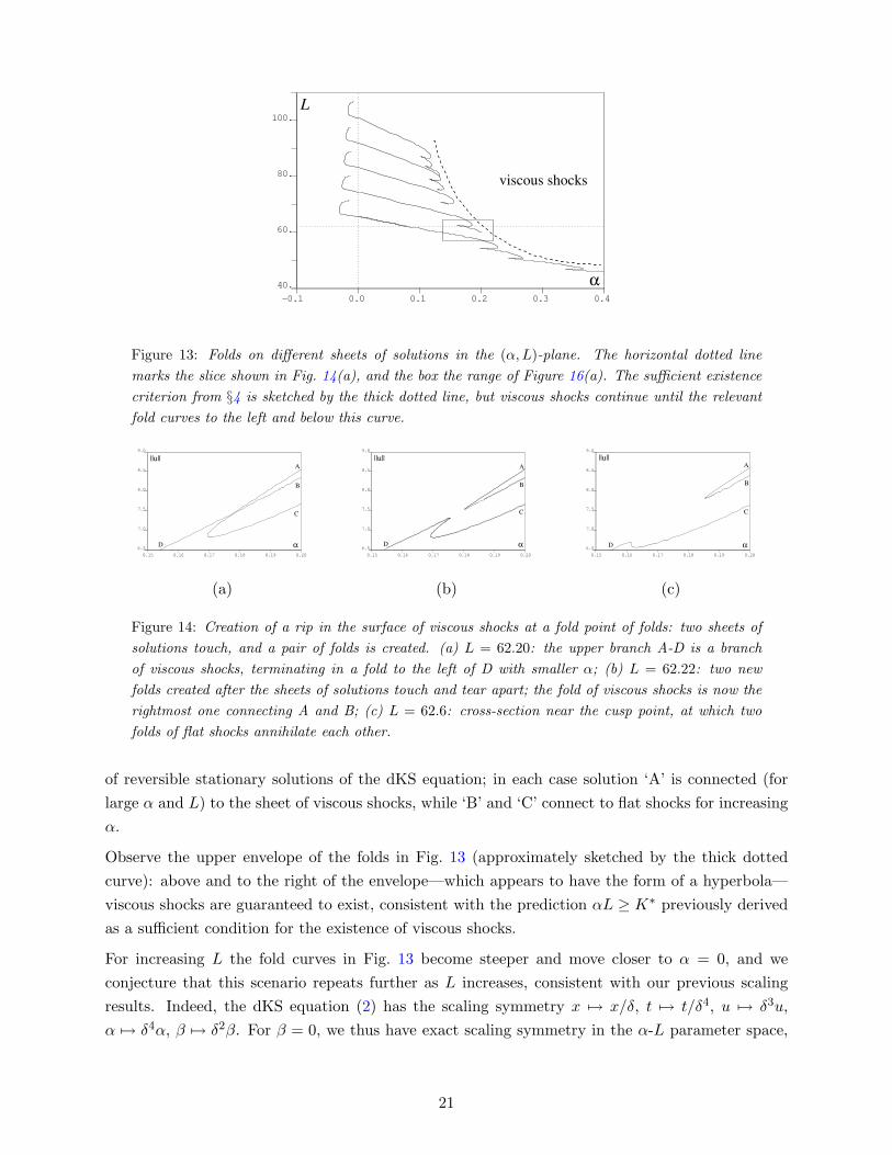
Folds of Viscous Shocks: For sufficiently large αL, we have seen that (for β = 2) there existsa two-parameter family of viscous shocks; we now consider the boundary of this sheet of viscousshocks in (α, L) parameter space. As mentioned above, for typical fixed period this boundary is afold, and we plot in Fig. 13 the numerical continuation of several such folds in the (α, L) plane. Thenature of the solutions along these folds changes with α, eventually terminating in roll solutions forα ≤ 0, while for α > 0 the corners of these curves are cusps, where two folds meet. Note that onlythe components of the fold curves intersecting α = 0 are relevant to viscous shocks, while beyondthe cusps for α > 0, the observed folds are the boundaries of sheets of flat shocks.

The intersection of these fold curves with α = 0 shows the path-connectedness of dKS viscous shocksand certain bubbles of the KS equation, but in all our computations the branch of a fold at α = 0does not connect directly to the sheet of viscous shocks for fixed L. Instead, it connects to rolls atα > 0 via flat and roll shocks. This can be partially understood by the points with horizontal slopein the graph of Fig. 13, for example at the dashed horizontal line: above the dashed line the foldof viscous shocks is the rightmost one, but below the dashed line it is the leftmost one. Indeed,at the degenerate fold where the curve has vanishing slope, the sheet of viscous shocks touches asheet of flat shocks and “rips” for increasing period, thus producing another curve of folds. Weillustrate this ripping process in Fig. 14, by showing various cross-sections at constant L of surfaces

20

-0.1 0.0 0.1 0.2 0.3 0.4

40.

60.

80.

100.

α

L

viscous shocks

Figure 13: Folds on different sheets of solutions in the (α, L)-plane. The horizontal dotted linemarks the slice shown in Fig. 14(a), and the box the range of Figure 16(a). The sufficient existencecriterion from §4 is sketched by the thick dotted line, but viscous shocks continue until the relevantfold curves to the left and below this curve.

0.15 0.16 0.17 0.18 0.19 0.20

6.5

7.0

7.5

8.0

8.5

9.0

C

B

A

D α

||u||

0.15 0.16 0.17 0.18 0.19 0.20

6.5

7.0

7.5

8.0

8.5

9.0

D

C

B

A

α

||u||

0.15 0.16 0.17 0.18 0.19 0.20

6.5

7.0

7.5

8.0

8.5

9.0

D

C

B

A||u||

α

(a) (b) (c)

Figure 14: Creation of a rip in the surface of viscous shocks at a fold point of folds: two sheets ofsolutions touch, and a pair of folds is created. (a) L = 62.20: the upper branch A-D is a branchof viscous shocks, terminating in a fold to the left of D with smaller α; (b) L = 62.22: two newfolds created after the sheets of solutions touch and tear apart; the fold of viscous shocks is now therightmost one connecting A and B; (c) L = 62.6: cross-section near the cusp point, at which twofolds of flat shocks annihilate each other.

of reversible stationary solutions of the dKS equation; in each case solution ‘A’ is connected (forlarge α and L) to the sheet of viscous shocks, while ‘B’ and ‘C’ connect to flat shocks for increasingα.

Observe the upper envelope of the folds in Fig. 13 (approximately sketched by the thick dottedcurve): above and to the right of the envelope—which appears to have the form of a hyperbola—viscous shocks are guaranteed to exist, consistent with the prediction αL ≥ K∗ previously derivedas a sufficient condition for the existence of viscous shocks.

For increasing L the fold curves in Fig. 13 become steeper and move closer to α = 0, and weconjecture that this scenario repeats further as L increases, consistent with our previous scalingresults. Indeed, the dKS equation (2) has the scaling symmetry x 7→ x/δ, t 7→ t/δ4, u 7→ δ3u,α 7→ δ4α, β 7→ δ2β. For β = 0, we thus have exact scaling symmetry in the α-L parameter space,

21

which persists in approximate form for fixed β > 0.

While numerical continuation fails, it appears that the fold curves may connect via small-amplituderolls for α < 0 to the trivial solution u ≡ 0 at α = 0. For α = 0, the fold curves connect to bubblesolutions of the KS equation; Fig. 1(a) shows one such solution. The curves intersect α = 0at approximately regular intervals, separated by ∆L/2 ≈ 4.42 ≈ 2π/

√2. This value equals the

wavelength of stationary oscillations about the trivial solution u = 0, with wave number ks =√

2(recall that the relevant part of the spectrum (3) for stationary solutions is λ = 0). Thus we canpropose an explanation for the discreteness and spacing of the fold curves in Fig. 13: We infer thatthe transition from one fold curve to the next at higher period L occurs, in the KS limit α = 0, viathe insertion of two (by reversibility) complete oscillations with wave number ks — asymptoticallyfor large L — into the bubble. The number of bubble oscillations for α = 0 may thus serve toparametrize the fold curves.

In summary, the transition from viscous shocks of the dKS equation to the KS equation is rathercomplicated, even in the context only of bifurcations of odd stationary periodic solutions. Fromthe point of view of the observed PDE dynamics, however, it is equally important to investigatethe stability of these stationary solutions.

Stability of Viscous Shocks: To supplement the existence results reported above, we discussthe stability of viscous shocks, and numerically compute boundaries of stability in a representativeregion in (α, L) parameter plane. To this end, we again use the continuation software auto, andadapt methods recently developed for the computation and continuation of spectra [26] to thisfourth-order PDE (2). We emphasize that our computations cover only a small part of parameterspace, but we expect that these reflect the general destabilization mechanisms when continuingviscous shocks to the KS limit α = 0. Our main results are plotted in Fig. 16, and we next describeour approach by continuation, referring to [26] for details.

We determine the stability of stationary solutions u(x) via the spectrum of the linearization L(u)of (2) in a solution, as in (6); on an L-periodic domain, we write this operator as Lper(u) :H4

per([0, L]) → L2per([0, L]). Note that unlike in the B-S equation (8), Lper(u) is generally not

self-adjoint (for u 6= 0), and its spectrum thus admits complex eigenvalues.

In order to numerically continue selected eigenvalues of Lper(u) [26] it is helpful to view its spectrumas part of the spectrum of L(u) cast as an operator LR(u) : H4(R) → L2(R). Recalling (7), wecompute curves of this spectrum for fixed (α, L) by continuing solutions of the boundary valueproblem

Vx = A(u, u1, λ)V , V (L) = eiγ V (0) (15)

in the parameter γ. To have full access to the points (u(x), u1(x)), we solve (15) simultaneouslywith the nonlinear system (5) with reversible boundary conditions u = uxx = 0; periodic boundaryconditions could also be implemented with appropriate modifications to break the reversible sym-metry and fix the phase. For γ ∈ 2πZ, (15) is precisely the eigenvalue problem for Lper(u), and itsfinite difference approximation was used to obtain initial conditions for the computations.

22

-0.3 -0.2 -0.1 0.0 0.1 0.2

0.0

0.5

1.0

1.5

2.0

2.5

3.0

3.5

4.0

λIm( )

Re( )λ

Figure 15: Part of the essential spectrum of a viscous shock with (α, L) = (0.15, 60) (only thespectrum in the upper half plane is needed, due to symmetry under complex conjugation). Bulletsare used to enlarge the four unstable, extremely small closed isolated curves, each of which containsan eigenvalue of Lper(u).

Figure 15 shows the result of one such computation, for L = 60, α = 0.15, in which we plot themost unstable curves in the spectrum of LR(u); each of the isolated parts of this spectrum containsan eigenvalue of Lper(u) [26], so that for these parameters the viscous shock is unstable, with fourcomplex conjugate pairs of eigenvalues with positive real parts.

Fixing γ = 0 and L, we next continue the solution u together with an eigenfunction V and eigenvalueλ of Lper(u) in α, and thus locate the onset of instabilities of specific eigenvalues, where Re(λ) = 0.By then fixing Re(λ) = 0 in the boundary value problem (15), continuation in (α, L) yields theparameter curve along which this eigenvalue crosses the imaginary axis. Note that other eigenvaluesmay become unstable independently, though this is not the case here.

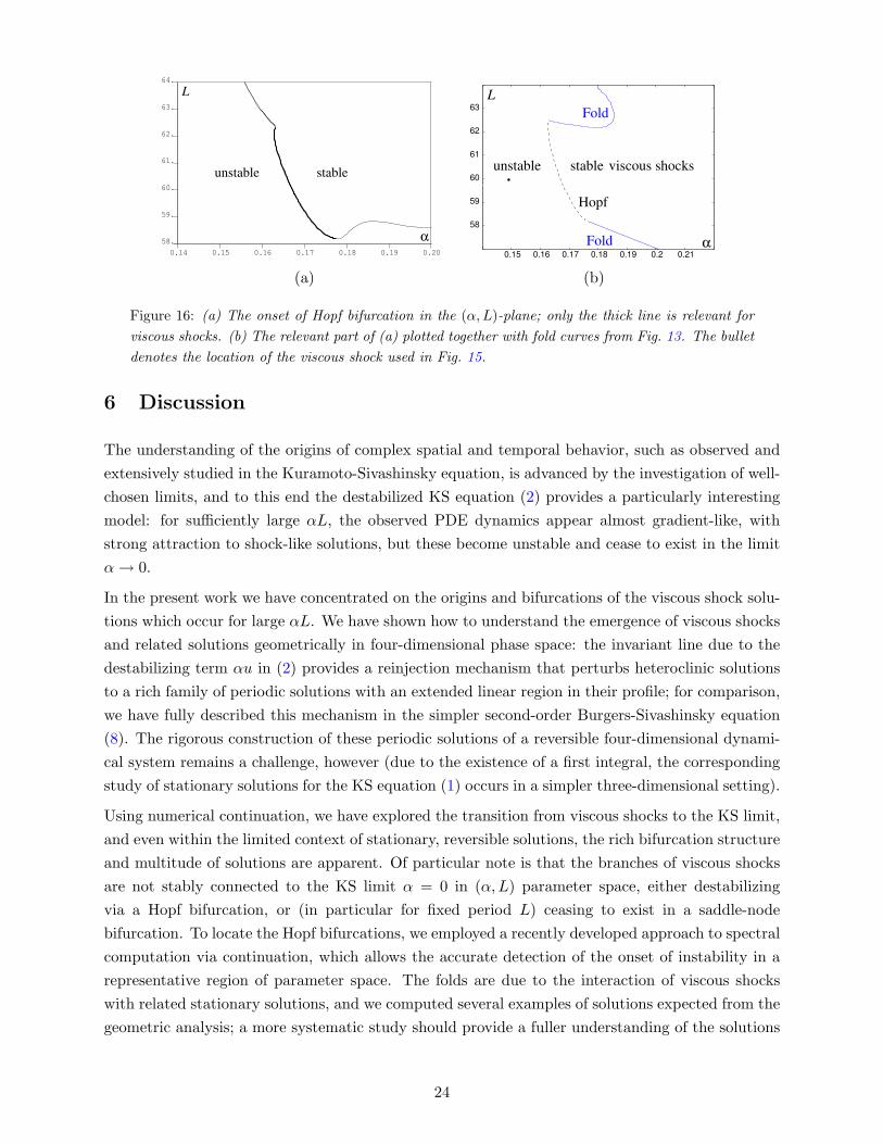
The spectrum plotted in Fig. 15 moves into the left half plane as α increases above α ≈ 0.17; thisstrict stability of the nontrivial eigenvalues implies exponential orbital stability of the underlyingviscous shocks, as observed in the PDE simulations. Interpreting this for decreasing α, there isthus a Hopf bifurcation of viscous shocks for L = 60, α ≈ 0.17. To locate the stability boundaryfor viscous shocks, we continue the Hopf bifurcation curves Re(λ(α, L)) = 0 in the (α, L)-plane. InFig. 16(a) we plot the resulting destabilization curve, which turns out to involve only one eigenvalue;here the thin lines are not relevant for viscous shocks, as they correspond to solutions on othersolution sheets, reached via a fold or cusp.

Combining the Hopf bifurcation curve of viscous shocks with the existence boundary consisting offold curves and cusp points plotted in Fig. 13, we obtain part of the boundary of stable viscousshocks in the (α, L)-parameter plane as plotted in Fig. 16(b). In particular, the Hopf bifurcationcurve connects two fold curves, and we conjecture that this structure persists throughout the (α, L)parameter plane. There is thus no connection of stable viscous shocks to the KS equation, as theirregion of existence is strictly bounded away from α = 0; rather, for decreasing α > 0 viscous shockseither cease to exist in a fold, or destabilize via Hopf bifurcations, as suggested by simulations ofthe PDE (2).

23

0.14 0.15 0.16 0.17 0.18 0.19 0.20

58.

59.

60.

61.

62.

63.

64.

L

α

stableunstable

58

59

60

61

62

63

0.15 0.16 0.17 0.18 0.19 0.2 0.21

stable viscous shocks

Fold

Fold

unstable

Hopf

α

L

(a) (b)

Figure 16: (a) The onset of Hopf bifurcation in the (α, L)-plane; only the thick line is relevant forviscous shocks. (b) The relevant part of (a) plotted together with fold curves from Fig. 13. The bulletdenotes the location of the viscous shock used in Fig. 15.

6 Discussion

The understanding of the origins of complex spatial and temporal behavior, such as observed andextensively studied in the Kuramoto-Sivashinsky equation, is advanced by the investigation of well-chosen limits, and to this end the destabilized KS equation (2) provides a particularly interestingmodel: for sufficiently large αL, the observed PDE dynamics appear almost gradient-like, withstrong attraction to shock-like solutions, but these become unstable and cease to exist in the limitα → 0.

In the present work we have concentrated on the origins and bifurcations of the viscous shock solu-tions which occur for large αL. We have shown how to understand the emergence of viscous shocksand related solutions geometrically in four-dimensional phase space: the invariant line due to thedestabilizing term αu in (2) provides a reinjection mechanism that perturbs heteroclinic solutionsto a rich family of periodic solutions with an extended linear region in their profile; for comparison,we have fully described this mechanism in the simpler second-order Burgers-Sivashinsky equation(8). The rigorous construction of these periodic solutions of a reversible four-dimensional dynami-cal system remains a challenge, however (due to the existence of a first integral, the correspondingstudy of stationary solutions for the KS equation (1) occurs in a simpler three-dimensional setting).

Using numerical continuation, we have explored the transition from viscous shocks to the KS limit,and even within the limited context of stationary, reversible solutions, the rich bifurcation structureand multitude of solutions are apparent. Of particular note is that the branches of viscous shocksare not stably connected to the KS limit α = 0 in (α, L) parameter space, either destabilizingvia a Hopf bifurcation, or (in particular for fixed period L) ceasing to exist in a saddle-nodebifurcation. To locate the Hopf bifurcations, we employed a recently developed approach to spectralcomputation via continuation, which allows the accurate detection of the onset of instability in arepresentative region of parameter space. The folds are due to the interaction of viscous shockswith related stationary solutions, and we computed several examples of solutions expected from thegeometric analysis; a more systematic study should provide a fuller understanding of the solutions

24

and bifurcations towards spatiotemporal chaos in the KS limit α → 0.

Acknowledgments

Much of this work was completed while JR was a PIMS postdoctoral fellow at Simon FraserUniversity and the University of British Columbia. JR thanks RW and Michael Ward for theirsupport. We acknowledge helpful conversations with Bjorn Sandstede and J. F. Williams. Thiswork was partially supported through an NSERC grant to RW, and SPP 1095 of the GermanResearch Foundation (JR).

References

[1] Cross, M., and Hohenberg, P., 1993, “Pattern Formation Outside of Equilibrium,”, Rev. Mod.Phys., 65, pp. 851–1112.

[2] LaQuey, R., Mahajan, S., Rutherford, P., and Tang, W., 1975, “Nonlinear Saturation of theTrapped-Ion Mode,” Phys. Rev. Lett., 34, pp. 391–394.

[3] Sivashinsky, G., 1977, “Nonlinear Analysis of Hydrodynamic Instability in Laminar Flames—I.Derivation of Basic Equations,” Acta Astron., 4, pp. 1177–1206.

[4] Kuramoto, Y., and Tsuzuki, T., 1976, “Persistent Propagation of Concentration Waves inDissipative Media far from Thermal Equilibrium,” Prog. Theor. Phys., 55, pp. 356–369.

[5] Misbah, C., and Valance, A., 1994, “Secondary Instabilities in the Stabilized Kuramoto-Sivashinsky Equation,” Phys. Rev. E, 49, pp. 166–183.

[6] Doelman, A., Sandstede, B., Scheel, A., and Schneider, G., 2005, “The Dynamics of ModulatedWave Trains,” preprint.

[7] Wittenberg, R. W., and Holmes, P., 1999, “Scale and Space Localization in the Kuramoto-Sivashinsky Equation,” Chaos, 9, pp. 452–465.

[8] Wittenberg, R. W., and Holmes, P., 2002, “Spatially Localized Models of Extended Systems,”Nonlinear Dynamics, 25, pp. 111–132.

[9] Michelson, D., 1986, “Steady Solutions of the Kuramoto-Sivashinsky Equation,” Physica D,19 pp. 89-111.

[10] Kent, P., and Elgin, J., 1992, “Travelling-Waves of the Kuramoto-Sivashinsky Equation:Period-Multiplying Bifurcations,” Nonlinearity, 5, pp. 899–919.

[11] Jones, J., Troy, W. C., and MacGillivary, A. D., 1992, “Steady Solutions of the Kuramoto-Sivashinsky Equation for Small Wave Speed,” J. Diff. Eq., 96 pp. 28-55.

[12] Lamb, J. S. W., Teixeira, M.-A., and Webster, K. N., 2005, “Heteroclinic Bifurcations NearHopf-Zero Bifurcation in Reversible Vector Fields in R3,” J. Diff. Eq., 219, pp. 78–115.

25

[13] Elgin, J. N., and Wu, X., 1996, “Stability of Cellular States of the Kuramoto-SivashinskyEquation,” SIAM J. Appl. Math., 56, pp. 1621-1638.

[14] Hooper, A. P., and Grimshaw, R., 1988, “Travelling Wave Solutions of the Kuramoto-Sivashinsky Equation,” Wave Motion, 10, pp. 405–420.

[15] Adams, K. L, King, J. R., and Tew, R. H., 2003, “Beyond-all-orders Effects in Multiple-ScalesAsymptotics: Travelling-Wave Solutions to the Kuramoto-Sivashinsky Equation,” J. Engin.Math., 45, pp. 197–226.

[16] Wittenberg, R. W., 2002, “Dissipativity, Analyticity and Viscous Shocks in the (De)stabilizedKuramoto-Sivashinsky Equation,” Phys. Lett. A, 300, pp. 407-416.

[17] Chate, H., and Manneville, P., 1987, “Transition to Turbulence via Spatiotemporal Intermit-tency,” Phys. Rev. Lett., 58, pp. 112–115.

[18] Goodman, J., 1994, “Stability of the Kuramoto-Sivashinsky and Related Systems,” Comm.Pure Appl. Math., 47, pp. 293–306.

[19] Bronski, J. C., and Gambill, T., 2005, “Uncertainty Estimates and L2 Bounds for theKuramoto-Sivashinsky Equation,” preprint arXiv:math.AP/0508481.

[20] Giacomelli, L., and Otto, F., 2005, “New Bounds for the Kuramoto-Sivashinsky Equation,”Comm. Pure Appl. Math., 58, pp. 297–318.

[21] Devaney, R. L., 1976, “Reversible Diffeomorphisms and Flows,” Trans. Am. Math. Soc., 218,pp. 89-113.

[22] McCord, C.K., 1986, “Uniqueness of Connecting Orbits in the Equation y(3) = y2 − 1,” J.Math. Anal. App., 114, pp. 584 - 592.

[23] Fenichel, N., 1979, “Geometric Singular Perturbation Theory for Ordinary Differential Equa-tions,” J. Diff. Eq., 31 pp. 53-98.

[24] Szmolyan, P., and Wechselberger, M., 2001, “Canards in R3,” J. Diff. Eq., 177 pp. 419-453.

[25] Doedel, E., Paffenroth, R. C., Champneys, A. R., Fairgrieve, T. F., Kuznetsov, Y. A., Olde-man, B. E., Sandstede, B., and Wang, X., 2002, “AUTO2000: Continuation and BifurcationSoftware for Ordinary Differential Equations (with HOMCONT),” Technical report, ConcordiaUniversity, Montreal.

[26] Rademacher, J. D. M., Sandstede, B., and Scheel, A., 2005, “Computing Absolute and Es-sential Spectra using Continuation,” IMA Preprint No. 2054, University of Minnesota, Min-neapolis, MN.

26