VISAGE - Dynpullig.dyndns.org/files/technical_description.pdf · Reservoir Simulator (SDRS), which links the VISAGE System to ECLIPSE. ... The science of geomechanics provides an

VISAGETechnical Description Version 2012.1

Proprietary notice

Copyright (c) 2012 Schlumberger. All rights reserved. Reproduction or alteration without priorwritten permission is prohibited, except as allowed under applicable law.

Use of this product is governed by the License Agreement. Schlumberger makes no warranties,express, implied, or statutory, with respect to the product described herein and disclaims withoutlimitations any warranties of merchantability or fitness for a particular purpose.

Trademarks & service marks

"Schlumberger," the Schlumberger logotype, and other words or symbols used to identify theproducts and services described herein are either trademarks, trade names, or service marks ofSchlumberger and its licensors, or are the property of their respective owners. These marks maynot be copied, imitated, or used, in whole or in part, without the express prior written permission oftheir owners. In addition, covers, page headers, custom graphics, icons, and other designelements may be service marks, trademarks, and/or trade dress of Schlumberger and may not becopied, imitated, or used, in whole or in part, without the express prior written permission ofSchlumberger.

VISAGE Technical Description

Table of Contents

1 Introduction to the VISAGE System .......................................................................... 11.1 Applications to Reservoir and Civil Engineering ....................................................................... 11.2 Main Features of the VISAGE System ......................................................................................... 2

Essential Features ....................................................................................................................... 2Materials Library ........................................................................................................................... 3Isoparametric Element Library ..................................................................................................... 3Solver Library ............................................................................................................................... 3Special Features .......................................................................................................................... 3Restart Facilities ........................................................................................................................... 4Analysis Capabilities .................................................................................................................... 4

1.3 Example Applications ................................................................................................................... 4Applications in Reservoir Engineering ......................................................................................... 4Applications in Civil Engineering .................................................................................................. 5

1.4 Conventions ................................................................................................................................... 51.5 Related Documentation ................................................................................................................. 5

2 Scientific Background ................................................................................................ 62.1 Introduction .................................................................................................................................... 6

3 Guidelines To Finite Element Modelling ................................................................... 93.1 Introduction .................................................................................................................................... 93.2 Idealization ..................................................................................................................................... 93.3 Subdividing the Structure ........................................................................................................... 103.4 Mesh Size ..................................................................................................................................... 103.5 Element Types ............................................................................................................................. 103.6 Element Shape and Size ............................................................................................................. 113.7 Solution Technique ..................................................................................................................... 113.8 Singularities ................................................................................................................................. 123.9 Loading ......................................................................................................................................... 133.10 Dynamics and Non-linearity ....................................................................................................... 133.11 Final Notes ................................................................................................................................... 13

4 Finite Element Types, Reduced And Exact Integration ......................................... 154.1 Introduction .................................................................................................................................. 154.2 Eight–Node Rectangular Finite Element Type .......................................................................... 164.3 Numerical Integration Over the Finite Element Area ................................................................ 184.4 ’Exact’ and ’Reduced’ Integration .............................................................................................. 20


i

Degrees of Freedom per Element .............................................................................................. 21Number of Constraints per Element ........................................................................................... 22

5 Finite Element Modelling Of Plasticity Within VISAGE ......................................... 275.1 Introduction .................................................................................................................................. 275.2 Physical Determination ............................................................................................................... 275.3 Visco–plastic algorithm .............................................................................................................. 29

’Visco–plasticity’ ......................................................................................................................... 305.4 Convergence Criterion ................................................................................................................ 325.5 Time Step Selection ..................................................................................................................... 335.6 Accelerators ................................................................................................................................. 35

Time–step Accelerator ............................................................................................................... 35Aitken’s Accelerator ................................................................................................................... 37

6 Invariant Yield Criteria .............................................................................................. 386.1 Mohr–Coulomb Criteria ............................................................................................................... 396.2 Critical State Criteria ................................................................................................................... 406.3 Chalk model ................................................................................................................................. 416.4 Modified Drucker–Prager model ................................................................................................ 446.5 CRITICAL STATE MODEL WITH HVSORLEV SURFACE .......................................................... 46

7 Jointed Rock and the Multilaminate Model ............................................................ 487.1 Introduction .................................................................................................................................. 487.2 ’Equivalent’ Material .................................................................................................................... 487.3 Constitutive Equations of Rock Mass ....................................................................................... 497.4 Elasticity Matrix Of Jointed Rock Mass ..................................................................................... 507.5 Non – linear Behaviour Of Jointed Rock Mass ......................................................................... 517.6 Multilaminate model for soils ..................................................................................................... 527.7 Joint and Multilaminate Yield Criteria ........................................................................................ 547.8 Mohr–Coulomb Criteria for Joints ............................................................................................. 547.9 Barton’s Criteria for Joints ......................................................................................................... 567.10 Mohr–Coulomb Criteria for Multilaminate Model ...................................................................... 577.11 Critical State Criteria for Multilaminate Model .......................................................................... 577.12 Critical State Criteria with Horslev failure and eccentricity for Multilaminate Model ........... 58

8 Modelling of Reinforced Rock ................................................................................. 618.1 Introduction .................................................................................................................................. 618.2 ’Equivalent’ Material .................................................................................................................... 618.3 Constitutive Equations of Reinforced Mass ............................................................................. 62


ii

9 Equation Solvers ....................................................................................................... 659.1 Introduction .................................................................................................................................. 659.2 Solution Techniques ................................................................................................................... 659.3 VISAGE solver options ................................................................................................................ 66

10 Consolidation Model ................................................................................................. 6710.1 Equations ..................................................................................................................................... 6710.2 General notes ............................................................................................................................... 70

11 Fracture/Fault Permeability Enhancement/Reduction .......................................... 7211.1 Permeability Enhancement ......................................................................................................... 7211.2 Permeability Reduction ............................................................................................................... 73

12 Additional Topics ...................................................................................................... 7712.1 Restarts ........................................................................................................................................ 78

Restarting a Nonlinear Analysis that has not Converged ........................................................... 78Description .............................................................................................................................. 78What to do .............................................................................................................................. 79

Using a Restart to Apply New Loads ......................................................................................... 79Description .............................................................................................................................. 79What to do .............................................................................................................................. 79

Using Restarts in Mining Operations .......................................................................................... 80Description .............................................................................................................................. 80What to do .............................................................................................................................. 80

12.2 Parametric Studies ...................................................................................................................... 81Changing Nonlinear Properties .................................................................................................. 81

Description .............................................................................................................................. 81What to do .............................................................................................................................. 81

Incrementing the Loads .............................................................................................................. 82Description .............................................................................................................................. 82What to do .............................................................................................................................. 82

Varying the Convergence Tolerance .......................................................................................... 82Description .............................................................................................................................. 82What to do .............................................................................................................................. 82

12.3 Use of Environmental Variables ................................................................................................. 83Changing Iterative Solver Tolerances ........................................................................................ 83

Description .............................................................................................................................. 83What to do .............................................................................................................................. 83

Perform an Elastic Analysis ....................................................................................................... 84Description .............................................................................................................................. 84What to do .............................................................................................................................. 84


iii

13 References and Bibliography .................................................................................. 8513.1 References ................................................................................................................................... 8513.2 Bibliography ................................................................................................................................. 8613.3 Further Reading ........................................................................................................................... 87


iv

1Introduction to the VISAGE

SystemThe VISAGE System consists of a Finite Element simulator and a graphical user interface formodel generation.Specific to reservoir engineering applications VISAGE Modeler is available for viewing reservoirgeometries and flow patterns generated by stress dependent reservoir simulations.VISAGE is currently ported on several hardware platforms and operating systems, includingMicrosoft Windows computers and Linux workstations.Parallel versions of the software are available, enabling large problems to be solved effectively andefficiently. The parallel option is based on a distributed memory architecture using MPI (messagepassing interface)

1.1 Applications to Reservoir and Civil EngineeringThe VISAGE System is a suite of finite element programs which offers scientists and petroleumengineers a robust, versatile, flexible and user controlled tool for solving a variety of complexengineering problems encountered in the oil industry. Fast and efficient, the system can beemployed to predict subsidence, compaction and pore collapse due to high pressure draw-downduring production operations. During water injection, micro fracture initiation and propagation,induced by thermal gradients and dynamic changes in the effective stress state, can be predicted,monitored and assessed. Post-frac productivity indices for vertical fracture completion can becalculated. An extensive non-linear material library provides a powerful tool for studying wellborestability problems. Exciting opportunities now exist for reservoir engineers to study the effect, onpreferred water flood directionality, of thermal gradients, stress magnitude and orientation, nowrecognized as key parameters for successful reservoir management. Coupled two and three phasereservoir simulations can be performed, using a recently developed three phase Stress DependentReservoir Simulator (SDRS), which links the VISAGE System to ECLIPSE. The new simulatorintegrates the disciplines of rock mechanics and petroleum engineering to assess the effect ofporous media deformation on fluid flow characteristics. Sophisticated 2-D and 3-D reservoir modelswith complex pre-defined distributions of faults are readily accommodated. During waterflooding,faults and fractures may become conduits of flow or indeed transmissibility barriers if sealing


Introduction to the VISAGE System 1

occurs. Furthermore, the evolution of fractures is constantly traced with hydraulic parameters beingupdated. Incorporating experimental data obtained from core samples to update permeabilities androck fabric characteristics, as fracturing develops, well orientations and locations can be optimized.The VISAGE System therefore provides a unique tool accounting for changes in the effectivestress state, neglected by most commercially available simulators.The increasing complexity of large civil engineering projects requires a fast flexible tool forgeotechnical analysis. The system offers extensive capabilities for the analysis, design andassessment of the structural integrity of dams, embankments, slopes, foundations, piles, retainingwalls and tunnels subject to static and/or dynamic loading. Implementing constitutive theories froman extensive non-linear material library the user is provided with a powerful tool for predictingsettlements and collapse, ensuring safe operational environments both in the short and long term.One phase capabilities accommodate groundwater modelling in environmental assessmentstudies. With the general enhancement and automation in mining techniques, ore is recoveredfrom ever increasing depths and the application of rock mechanics plays a crucial role. In complexmining operations the stability of stopes and caverns, during excavation and back filling, can bepredicted for different mining sequences. Alternative plans can therefore be reviewed quickly toensure safe environments for excavation, whilst maximizing ore body recovery. In the design ofunderground caverns for the storage of nuclear waste complex geological features of rock massesand thermo-mechanical regimes can be readily incorporated in the model simulation. The effect ofground movements along rock joints and discontinuities can therefore be accounted for and safetyfactors determined.

1.2 Main Features of the VISAGE SystemThe main features of the VISAGE System are outlined in the following sections:• Essential Features.• Materials Library.• Isoparametric Element Library.• Solver Library.• Special Features.• Module Library.• Restart Facilities.• Analysis Capabilities

Essential Features• Modular design.• Large 2–D and 3–D grids.• Speed.• Flexibility and efficiency.



Materials Library• Mohr Coulomb.• Von–Mises.• Tresca.• Drucker–Prager.• Modified Drucker–Prager with Cam Clay flow potential surface.• Hoek and Brown.• Critical State using Modified Cam Clay Model.• NGI chalk model for simultaneous plasticity and creep.• Mohr–Coulomb for joints and faults.• Barton’s theory for joints.• Multi–laminate with Mohr Coulomb.• Multi–laminate with Hvorslev’s surface and modified Critical State cap.• Multi–laminate with Critical State.

Isoparametric Element Library• 2–D / 3–D 2 and 3 noded beams.• 2–D 3 and 6 noded triangles.• 2–D 4, 8 and 9 noded quadrilaterals.• 3–D 8 and 20 noded bricks.• 3–D 6 and 15 noded prisms.• 3–D 4 and 10 noded tetrahedra.• 2–D and 3–D infinite elements

Solver Library• Direct symmetric/asymmetric.• Out–of–core direct symmetric/asymmetric.• Iterative symmetric/asymmetric.• Iterative symmetric/asymmetric with AMG methods.

Special Features• User friendly.• Element library.• Solver library.• Materials library.



• Preprocessors.• Postprocessors.• Propriety interfaces.• Parallel versions.• Shared and distributed memory.• Hardware independent.• Restart facilities.• Help text.

Restart Facilities• Restarting from different loads.• Restarting nonlinear analyses that have not converged.• Applying/updating loads.• Restarting between modules.

Analysis Capabilities• Steady state.• Creep.• Fully coupled one phase flow (consolidation).• Jointed and reinforced rock masses.

1.3 Example ApplicationsExamples of applications of the VISAGE System are outlined in the following sections:• Applications in Reservoir Engineering.• Applications in Civil Engineering.

Applications in Reservoir Engineering• Waterflooding.• Wellbore stability.• Subsidence.• Compaction.• Thermal fracturing.• Structural geology.• Multiphase flow.• Well location optimization.



Applications in Civil Engineering• Slope Stability.• Back filling.• Excavation.• Piles.• Tunnelling.• Slopes and embankments.• Foundations.• Reinforcements.

1.4 ConventionsThe following typographic conventions are used in this manual:Examples of commands typed in or the contents of a file are shown boxed and in this font. Forexample:

C> CD VISAGE

Note: This symbol is used for indicating significant points. A note.

• a bullet indicating brief explanatory text.• a bullet indent. Normally indicating a series of related text.

CAUTION: A WARNING box is important and users should take note of all warning messages.

1.5 Related DocumentationThe following manuals are intended to be used in conjunction with this manual:• ECLIPSE 100/300 Reference Manual.• VISAGE Reference Manual.• VISAGE Modeler User Guide.



2Scientific Background

2.1 IntroductionThe science of geomechanics provides an extensive field for research, especially with recentadvances in technology. New, complicated, experimental devices and faster and more powerfulcomputers have assisted in the venture, yielding improved and elegant solutions to geotechnicalproblems. Among the numerical techniques that have emerged as an adequate means for thesolution of geomechanics problems, is the finite element method. However, the development offinite element techniques in geomechanics has remained largely in the academic environment withminimal practical application. This is due either to uncertainties in the basic finite elementtechniques in describing soil/rock behaviour or the development of complex numerical algorithmsto approximate various soil/rock aspects which were not easily understood by engineers.A finite element system, the VISAGE System, which is applicable to most geotechnical problemsencountered in engineering practices, has now increased the engineer’s confidence in obtainingcomplex solutions efficiently. Thus in determining quantitative results from various types ofanalyses, a better understanding of the behaviour of structures can now be obtained.The concept of a numerical approach that will reproduce the stress/strain/volume change behaviorof a geomass under three–dimensional stress states, arbitrary loading paths and drainageconditions, is still a long way off, despite the extensive research efforts and the development ofsophisticated constitutive models. Even if such an approach existed, it would be unwieldy and toocomplex. It is therefore necessary to isolate the salient features that govern the soil/rock behaviorin a particular problem.Generally speaking, soils/rocks behave in a more complicated manner than a simple elastic theorycan predict. The main physical feature of this behavior is the irrecoverability of strains. Consider inthe daigram below, a typical stress–strain curve obtained by a drained triaxial test.The numerical interpretation of the relationships between stresses and strains are complicatedfunctions depending on the coefficients selected to represent the soil behavior. In addition soils arefar from uniform and variations in properties occur from stratum to stratum and from site to site.This variability makes analysis in geomechanics difficult and somewhat subjective.


Scientific Background 6

Figure 2.1. Stress–Strain Behaviour of Soil

It has been shown in the past that simple non–linear numerical models can take into accountstress–strain relationships and therefore predict soil/rock behavior better than most elastic models.The simplest non–linear stress–strain behavior available for the prediction of collapse loads ofdrained soil masses is the elastic, perfectly plastic. In this theory, a ’yield surface’ separates stressstates, which give rise to both elastic and plastic (irrecoverable) strains. More accurately, thismeans that soils/rocks behave elastically until a ’failure criterion’ is violated, at which point, plasticbehavior occurs.Two basic theories have appeared recently in the literature for predicting collapse loads; ’initialstress’ and ’initial strain’. It is a matter of choice of which of these numerical approaches to use, tosuccessfully apply the ’yield criteria’ established in geomechanics in the early 50’s by Drucker,Prager, Mohr–Coulomb, Tresca and Von–Mises, who predicted collapse loads using either



associated or non–associated flow rules. The ’yield criteria’ take into account simple plasticconstitutive properties such as the cohesion strength, c’, and the friction angle, Φ.A representative of ’initial stress’ methods is that of ’tangential stiffness’, whilst the ’visco–plastic’method is an example of ’initial strain’. It is the ’visco–plastic’ approach that has been developed inthe VISAGE System, since it provides all the necessary attributes dictating the steady–state andtransient behavior of soil/rock masses.Whilst searching for accuracy, different researchers have applied different finite element types topredict collapse loads. Initially there was controversy as to whether ’exact’ or ’reduced’ integrationshould be considered in certain problems, not only to improve the performance of the finite elementmethod, but also to obtain more accurate collapse loads. Particular difficulties were encountered inaxisymmetric problems.Simple mathematical considerations show that collapse loads could be predicted, ifincompressibility is satisfied at every point within the finite element domain. This is achieved, whenthe number of constraints per element, as derived from compatibility considerations, is lower thanthe number of degrees of freedom. The incompressibility ratio defined as (degrees of freedom)/(constraints) per element must be at least unity. If this condition is not satisfied, theincompressibility theorem is violated and collapse cannot be predicted. Correct choice of finiteelement type is therefore important.The applicability of an axisymmetric element to predict collapse loads is dependent upon on thegauss point scheme used for numerical integrations. Mathematically the compressibility theorem issatisfied at the gauss points for ’reduced’ integration only. ’Exact’ integration schemes should notbe used for axisymmetric elements.



3Guidelines To Finite Element

Modelling

3.1 IntroductionIn the context of the finite element method, an actual structure or continuum is replaced by anequivalent idealized structure composed of discrete elements, referred to as finite elements. Theseare connected together at a number of specific nodal points. By assuming displacement fields orstress patterns within an element it is possible to derive a stiffness matrix relating the nodal forcesto the nodal displacements within an element. The stiffness matrix of the assemblage of elementscan be formed by considering the nodal contributions in an overall stiffness matrix of each of theindividual elements. If conditions of equilibrium are applied at every node of the idealized structure,a set of simultaneous algebraic equations can be formed, the solution to which provides all thenodal displacements. These in turn are used to determine all the internal stresses. The majority offinite element packages assume linear elastic small elastic theory. The VISAGE System can offernon–linear, small strain, small and large displacement capabilities.

3.2 IdealizationFirst of all, in any analysis, it is necessary to discretize the continuum, by subdividing the structureinto one, two or three–dimensional finite elements by fictitious lines and/or surfaces. Thus, thestructure is now represented by an assemblage of simple geometric shapes rather than having acomplex geometric outline. The elements are assumed to be interconnected at a discrete numberof nodal points situated at the element boundaries. The way the structure will be meshed, willdepend on:• The physical nature of the structure itself.• The element types to be used.• The extent of the area of intersect.• The type of analysis: static, dynamic, potential, eigenvalue, thermal or non–linear.• The cost of running the analysis and the way the loads are applied.


Guidelines To Finite Element Modelling 9

3.3 Subdividing the StructureIt is normally trivial to decide how to subdivide the structure into finite elements by the physicalspecification of the structure. With frame structures such as oil–rigs or buildings there is an obviouscorrespondence between real and idealized beams. In more discontinuous structures such as anearth dam, the obvious breakpoints are at the material boundaries.There are two aspects that should always be looked for initially: symmetry and repetition.In many structures, symmetry can be used to significantly reduce the size of the problem to besolved. The use of such a condition reduces, not only the number of elements involved, but willnormally significantly reduce the bandwidth of the equations to be solved also. As the cost of thesolution is proportional to the square of the bandwidth (for skyline solvers), this is a very importantfactor. With symmetry, the symmetric plane is constraint to remain planar. This technique may alsobe used with radial symmetry such as in discs. Loading will also need to be symmetric although itis sometimes possible to use loading combinations to give results for asymmetric loads onsymmetric structures, provided that an elastic analysis is performed.However, the VISAGE System incorporates highly sophisticated equation solvers which assist inovercoming some of these problems. See the chapter on equation solvers.

3.4 Mesh SizeApart from the constraints imposed by the physical nature of the structure, the mesh size will bechosen to provide for three major factors. The overriding requirement is that the element must becapable of mathematically representing the physical area it defines to the degree required. Thus, itmight possible to mesh for a large number of fairly simple elements or a much smaller number ofhigher order elements. It is for this reason that higher order elements have been adopted for usewithin the VISAGE System.The basic mesh may then be refined or degenerated depending on whether it contains an area ofinterest. With frame structures, the overall response is normally looked for and no local refinementis called for. In solid body analysis there will often be a region of main interest, this will need tohave an adequately refined mesh. Elsewhere it is only necessary to ensure that the load willdiffuse correctly into the area. Hence mesh refinement may well be necessary in the areas ofrestraint or localized load application to ensure load diffusion is correct. In the interface region it willalso be necessary to ensure a gradual change in element size to ensure individual elements canperform correctly.

3.5 Element TypesThe VISAGE System uses the ’displacement’ method for its basis for finite element analyses.According to this method, the displacements are chosen as the prime unknowns, with the stressesbeing determined from the calculated displacement field. This method is used by most finiteelement packages. In this technique, the displacement of the system of nodes is assumed to haveunknown values only at the nodal points so that variation within any element is described in termsof the nodal values by means of interpolation functions, normally referred to as the ’shapefunctions’. It is important to realize that these functions governing the performance of an elementare incorporated between nodes and hence extreme distortion of any element may give strangeresults or fail due to a mathematically contorted function. The strains within any element may be



expressed in terms of the element nodal displacements where the strains will be composed of thederivatives of the ’shape functions’. The element stresses are calculated from the strains in amanner which ensures the satisfaction of equilibrium and plasticity equations. Provided that theelement ’shape functions’ have been chosen so that no singularities exist in the integrands of thefunctional, the total potential energy of the continuum will be the sum of the energy contributions ofthe individual elements. The summation of the contributions, when equated to zero, results in asystem of equilibrium equations for the complete continuum. These equations are then solved byany standard technique to yield the nodal displacements.The element formulations will, for the displacement method, ensure displacement continuity acrossboundaries of elements. Hence it is essential that all nodes at element boundaries are fullyconnected to adjacent lines of nodes, otherwise forces will not be transmitted through thecontinuum correctly and element edges will be allowed to deform locally, to pull apart, or overlap.

3.6 Element Shape and SizeA prime requirement in using finite elements is that they are not forced beyond the limits of theirgoverning mathematics. Hence the use of a higher order element is likely to allow the user muchmore flexibility and return greater accuracy. It is probably worthwhile to consider the variouselements into two very broad categories of lower and higher order elements. The lower orderelements will probably have linear variation of geometry stress and strain whilst the higher orderelements will have correspondingly higher order variations. Lower order elements will thereforeneed to be used in greater numbers to approach the degree of accuracy achieved when using anisoparametric element.How large an element is and its shape will be governed by attempting to fit a meshing scheme tothe structure. The prime requirement for this will probably be to define a coarse mesh, except atthe area of interest, for reasons of economy. The coarse mesh will therefore need to cope with theload diffusion through the structure. The fine mesh will need to give enough detail and thenecessary stress components output for the engineer to decide how the structure is performing inthat area.In defining these two areas and the transition region, some elements are likely to be deformed tomap the structure adequately. The simple, lower order elements will not perform well whenremoved from aspect ratios of 1:1 and simple, lower order elements should certainly not be usedwhen being pulled more into a ’spiked’ shape. Higher order elements can cope with an order ofmagnitude greater distortion. Thus the eight noded elements can often be given with aspect ratiosof up to 1:7, whilst the equivalent brick element can rise to orders of 1:10 and cause littledegradation in performance.Whilst working with these general guidelines it must be remembered that between the nodal pointsdefining the element is the ’shape function’. If these points are positioned so as to cause peculiaredge shapes, they may cause integration points to move outside the relevant boundary. Such anoccurrence causes a singularity of the element and the program execution will normally abort.

3.7 Solution TechniqueThere are three main solution techniques used within the finite element method. They are the in–core skyline, the out–of–core skyline and the iterative solvers. In the skyline solutions the centralnon–zero diagonal part of the stiffness matrix defining the structure is stored. This is then solved as



a whole or in parts. If it is solved in parts, then an out of core solver is said to be in use. The out ofcore method is used for larger skyline problems.It is particularly important for the banded solution to keep the width of the band as low as possibleas the solution time will be proportional to the square of the bandwidth. The semi–bandwidth will bedefined by the maximum number difference in any element plus one multiplied by the number ofdegrees of freedom being used. To achieve the optimum bandwidth, the REORDER interface isprovided as part of The VISAGE System.The iterative solvers are independent of element and/or nodal ordering sequence. The stiffnessmatrix must be positive definite and, for large problems, provides an effective solver from both theCPU and memory management points of view.There is a threshold above which the iterative solvers are much faster than the skyline solvers.Below this threshold, the skyline provides a faster solution as it requires only one inversion of theglobal stiffness matrix. This threshold value is dependent on the number of elements, elementtypes and number of dimensions. It also depends on the memory available on the machine.As a general rule it is always good practice to number the structure for optimum bandwidth andfrontwidth. This will enhance the ability of The VISAGE System to solve problems that demandsubstantial memory stacks, although this is not important for the iterative solver.

3.8 SingularitiesThe accuracy of the solution will be dependent upon the conditioning of the equations the solverhas been asked to solve. In physical terms this can be regarded as the relative stiffnesscontributions given by the equations involved. Thus if one area of the matrix appears to be dividingthe structure into two very stiff regions with a very flexible region, the solution may be highlyinaccurate. There would appear to be five main causes commonly associated with this problem:non–fixed structures, distorted elements, unintentional multi–structures, bad modelling choice ofelements and structures on flexible mountings.It is a requirement for all these solutions that the structure is not free in space and so restraintsmust be introduced to prevent this. It is important however not to overstrain the structure; it shouldbe free to deform in a real physical manner.If, when using constraint equations, which are forcing freedoms to have their displacements relatedto others, and releasing certain freedoms, it is important not to totally release that part of thestructure. This may also occur if coincident nodes or gaps in nodes are used and some elementsare not correctly joined.Distorted elements are a frequent problem, necessitating remodelling. If the elements are used inan unacceptable fashion it can appear to the solution that a local region of practically zero stiffnessoccurs hence causing singularity. This may be caused by the elements physical geometry and thevalues given for it to build its elasticity matrix such as Young’s Modulus or Poisson’s Ratio. Thiscould also happen if an element is used in an inappropriate place, for example a thin elementwhere large stresses needed to be transmitted. Having very large elements next to very smallelements can also cause similar problems.Occasionally structures need to be modelled that physically do have weak areas supporting stiffstructures. Support conditions for slung bodies often have this problem where the supports usedmay be varied along the length. Here all that can be done is take great care in checking thereaction forces and attempting to define the structure so that numerically the solution progresses



from “stiff” equations to the “weaker” equations by judicious use of the numbering orsubstructuring. This averts sudden jumps in relative stiffness.

3.9 LoadingAll packages provide for a range of loading types. Point loads and distortions are the basis of allloads as applied onto the final structure. However, more sophisticated patterns of pressure andbody forces can be applied using the internal element shape functions and hence equivalent nodalloads will be calculated to give the correct mathematical distribution to suit that function. If this wasnot used, dividing loads on an eight node face equally would tend to cause high distortion at thecorner nodes in comparison with mid–side nodes.

3.10 Dynamics and Non-linearityFor the purposes of these notes neither dynamics and non–linearities can be discussed further.The user must make certain to read some of the recommended literature on these subjects.However, the user must be aware that these techniques cost a minimum of an order of magnitudemore than linear static or thermal analyses in terms of CPU time and must ensure that they takegreat care in both data preparation and theoretical understanding of the implications of the basicsof VISAGE.Dynamic analyses can normally be made with a much cruder model than for static analyses. Oftenthe number of degrees of freedom considered at the nodes can also be reduced. The mass matrixfor the structure can either be described with only the diagonal terms considered (lumped mass) orin full (consistent mass). The lumped mass approach is commonly used for most analyses and willnormally produce satisfactory results.Non–linearity can be both material and geometric and some experience and care is needed toguide the program to a reasonable solution.

3.11 Final NotesIn deciding on model selection, appropriate considerations are required to ensure that it candescribe the physical condition with the required accuracy. Make sure that the answers that areobtained in a visual form could be used with some engineering judgement. Mesh the structure asevenly as possible avoiding any gross distortion of element shape, but refining to accommodatelocal high stress and loading as necessary.

Note: Care must be taken in fixing the structure globally, in a manner that it will allow it move as inpractice. An attempt must be made to minimize the bandwidth and for that several tools areavailable. All the relevant structure must be included in the model.

Note: Checks must be performed on most input data, so that it conforms to the model to beanalysed and ensure that it conforms to the program input specification.



CAUTION: Inadequate checking is the biggest single cause of error.



4Finite Element Types, Reduced

And Exact Integration

4.1 IntroductionIn many engineering problems, predictions of stress–strain distributions in elastic or elasto–plasticcontinua are required. Finite element solutions are commonly sought in plane stress and planestrain and axisymmetry, for plate bending and shells. In applying the finite element technique it isassumed that:• The continuum is discretized by lines or surfaces into a number of finite elements.• The elements are assumed to be interconnected at a discrete number of points called nodes

which are situated at the elemental boundaries.• The deformation at a node is described by deformation variables which are the unknown

degrees of freedom at the node.• A set of shape functions is chosen to define uniquely, the state of deformation within each finite

element, in terms of nodal displacements.• The shape functions therefore define uniquely, the state of strain within an element, in terms of

the nodal displacements. The strains together with any initial strains and the constitutiveproperties of the material, define the status of stress throughout the element.

• An elemental stiffness matrix relates the degrees of freedom to a system of forces concentratedat the nodes which equilibrate externally applied loads.

• Assembling the stiffness matrices for all the elements gives the stiffness matrix for the structure.• The structural stiffness matrix relates the unknown degrees of freedom to the applied forces or

pressure loads at the boundaries.Although the finite element method is a numerical discretization technique for modelling thecontinuum, correct collapse loads may be predicted for numerous types of problems, nowheremore apparent that in geotechnics.A solution will converge to an exact collapse load, when the compressibility theorem is satisfiedand the integration order is such that the volume of a finite element is determined exactly. The


Finite Element Types, Reduced And Exact Integration 15

number of integration points implemented in a given procedure now becomes important togetherwith the shape functions used to describe displacement variations within the element. The conceptof shape functions is discussed in Section 15.2.2 where the 8 noded isoparametric element isintroduced. In calculating volumes, the following should be considered:• Shape functions and their derivatives should be continuous within the element they describe.• Shape functions and their derivatives should allow nodal displacements caused by rigid body

translations and rotations to occur, without straining the element and without changing thestrain energy within the element.

• Shape functions and their derivatives should allow all states of uniform strain to exist within theelement.

• Shape functions and their derivatives should satisfy internal compatibility within the element andalso maintain compatibility of displacements between adjacent elements at the nodes and alongthe boundaries.

The ’shape functions’ uniquely define the state of strain within the finite element, provided theincompressibility theorem:

ϵr + ϵz + ϵ θ = 0 Eq. 4.1

is satisfied. Under plane strain conditions , thus the number of constraints, as imposed byelemental compatibility, is less than the number required for axisymmetric conditions. It is thereforemore difficult to predict collapse loads in axisymmetry. More kinematics rules require the definitionof more variables to represent the ’shape functions’ adequately. To satisfy equation [1] knowingthe ’shape functions’ of the finite element, the lowest number of integration points must be definednecessary to evaluate the volume of this element. If the number of integration points is such that itallows the determination of equation [1] throughout the element area, the integration rule isan ’exact’ type. If a lower number of integration points is specified than that required by ’exact’integration, then a ’reduced’ type of integration is considered. This ’reduced’ type of integrationsatisfies equation [1] at the integration points only and provision must be made in order for it to besufficient to compute the volume of the element as accurately as the ’exact’ type does. Thecontroversy of whether a specific finite element type is capable of predicting collapse loads istherefore confined to comparisons between ’reduced’ and ’exact’ types of integration formulae.This problem is now investigated for the 8–node isoparametric quadrilateral finite element, wherethe spatial variations of coordinates and displacements within the elements are computedusing ’shape functions’ defined in a local coordinate system.

4.2 Eight–Node Rectangular Finite Element TypeThe 8–node rectangular isoparametric element has been one of the most commonly used finiteelements in the literature in the last ten years. The local coordinate system used to define theshape functions of the element and the gauss point locations for the numeric integrations areshown below.



Figure 4.1. Finite Element Representation of an 8–Node Quadrilateral Element

The ’shape function’ polynomials in the local coordinate system at the corner nodes are defined:

N1 = 14 (1 − ξ)(1 − η)( − ξ − η − 1)

N3 = 14 (1 − ξ)(1 + η)( − ξ + η − 1)

N5 = 14 (1 + ξ)(1 + η)( + ξ + η − 1)

N7 = 14 (1 + ξ)(1 − η)( + ξ − η − 1)

Eq. 4.2

whilst at the midside nodes:

N2 = 12 (1 − ξ)(1 − η 2)

N4 = 12 (1 − ξ 2)(1 + η)

N6 = 12 (1 + ξ)(1 − η 2)

N8 = 12 (1 − ξ 2)(1 − η)

Eq. 4.3

Due to symmetry, the ’shape functions’ of an 8–node rectangle, are simple functions of the localaxes ξ and η. Thus, their derivatives are very easy to extrapolate from the above set of equations.In plain strain and axisymmetry the calculation of elemental volumes using both 2x2 and 3x3Gaussian integration procedures is exact. In plain strain conditions the compressibility theorem issatisfied for both 2x2 and 3x3 rules and correct collapse loads are therefore predicted which ever



rule is implemented. However in axisymmetry the use of higher order 3x3 rules violates thecompressibility theorem and lower order rules must be used to predict collapse loads accurately.

Note: To predict collapse loads in axisymmetric problems ’reduced’ integration rules must beimplemented.

4.3 Numerical Integration Over the Finite Element AreaNumerical integration procedures for quadratic elements are well known in the literature and willnot be discussed here. Instead attention is focused on numerical integration procedures fortriangular elements. It now becomes an immense and often highly complicated mathematical taskto determine the number of the integration points and their location such that the elemental areascan be determined exactly and the compressibility theorem satisfied. This is particularly the casefor 15–node cubic strain triangles.It has been proved that the rank preservation condition can be achieved over triangular areas, if aclass of symmetric, positive definite matrices is used in the finite element analysis and the ’shapefunctions’ at each node are polynomials, dependent on the domain variables.Consider now the element stiffness matrix:

KM = ∫ vB T D B d V Eq. 4.4

where:[.B] is the element strain–displacement matrix[D] is the elastic stress–strain matrixandV represents the domain of integration.Applying the transformation:

B * = U * B Eq. 4.5

where [U*] is given by:

D = U * T U Eq. 4.6

We obtain:

KM = ∫ VB * T B * d V = ∑

i=1

p ∫ VB *

iT B *

id V Eq. 4.7

Standard finite element representation requires that:

B *i

= N i{a }i Eq. 4.8



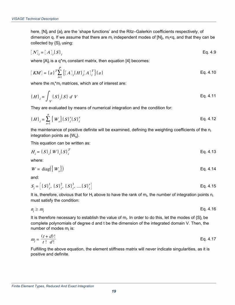
here, [N]i and {a}i are the ’shape functions’ and the Ritz–Galerkin coefficients respectively, ofdimension q. If we assume that there are mi independent modes of [N]i, mi<q, and that they can becollected by {S}i using:

N i = A i{S}i Eq. 4.9

where [A]i is a q*mi constant matrix, then equation [4] becomes:

KM = {a }T∑i=1

P { A i{H }i A iT }{a } Eq. 4.10

where the mi*mi matrices, which are of interest are:

{H }i = ∫ V{S}i{S} d V Eq. 4.11

They are evaluated by means of numerical integration and the condition for:

{H }i = ∑s=1

n {Ws}{S}is{S}i

s Eq. 4.12

the maintenance of positive definite will be examined, defining the weighting coefficients of the niintegration points as {Ws}.

This equation can be written as:

H i = {S}i{W }i{S}iT Eq. 4.13

where:

W = diag({Ws}) Eq. 4.14

and:

Si = {S}i1, {S}i

2, {S}i3, ....{S}i

s Eq. 4.15

It is, therefore, obvious that for Hi above to have the rank of mi, the number of integration points nimust satisfy the condition:

ni ≥ mi Eq. 4.16

It is therefore necessary to establish the value of mi. In order to do this, let the modes of {S}i becomplete polynomials of degree d and t be the dimension of the integrated domain V. Then, thenumber of modes mi is:

mi = (t + d)!t ! d ! Eq. 4.17

Fulfilling the above equation, the element stiffness matrix will never indicate singularities, as it ispositive and definite.



4.4 ’Exact’ and ’Reduced’ IntegrationA criterion for predicting accurate collapse loads using traditional displacement formulations ispresented in this section. It is shown that the compressibility theorem must be satisfied and that thenumber and location of the integration points must be chosen correctly.The principle of virtual work is fundamental to structural mechanics and is applicable to both staticand dynamic problems. The virtual work principle may be derived independently of the mechanicalproperties of the material in use and is therefore valid for any body state – solid, liquid, gaseous –whether it is elastic or plastic. For a body in equilibrium the acting forces do not initiate anymovements of the body. No work is done by a system of forces in equilibrium. The term virtualdisplacement, signifies a small imaginary displacement from the position of equilibrium, which doesnot violate the geometrical conditions or constraints imposed on the movements or deformationpatterns of the body. This virtual displacement could occur, but does not. Subject to this restriction,the virtual displacements can be quite arbitrary.The deformation rate and variation of strains and stresses play a central role in the derivation ofvirtual work equations. Applying the principle of virtual work to structural mechanics, stresses andstrains must satisfy the following equation:

∫ sT i

.ui.

d S = ∑elem

∫ v σ.

ij ε.

ij d V Eq. 4.18

where :σij is the stress rate following the prescribed constitutive law in terms of the current stress

ui denotes a velocity field, which may or may not be independent of the stress field

εij is the strain rate field associated with the velocity ui and Ti represents the surface traction ratesover the area S.Expressing the stresses and strains shown above in terms of deviatoric stresses it follows that:

σij.

ε.

ij = s.ije

.ij + 1

3 σ.

kk ε.

kk Eq. 4.19

where:eij is the deviatoric strain rate

andsij is the deviatoric stress rate.

As the plastic deformation is assumed purely deviatoric, the hydrostatic term 1/3σkk can beexpressed as follows:

σ.

kk = 3K ε.

kkEq. 4.20

Use the above equations, we finally obtain:

∫ sT i

.ui.

d S = ∑elem

∫ v(sij.e.ij + K (ε

.kk)2) d V Eq. 4.21



in which K is the bulk Modulus of the material which can be expressed in terms of the Young’sModulus E and Poisson’s ratio ν as follows:

K = E3(1 − 2v) Eq. 4.22

and εkk is the dilational strain increment.

Plasticity theory requires:

ε.

kk = 0 Eq. 4.23

Which is the incompressibility theorem expressed and indicates that the plastic work done on anelement of plastic material by the ’yield’ stress may be calculated by summing the work done byeach stress component. Equation [15.2.4.6] for statically admissible stress fields σkk , becomes:

∫ sT i

.ui.

d S = ∑elem

∫ v(sij.eij

. ) d V

Solutions obtained using the finite element method are therefore admissible provided that theprinciple of virtual work is satisfied that is:• The incompressibility theorem is satisfied over the finite element domain.• All stress strain points lie on the ’yield’ surface for all integration points of the mesh.If those two requirements are met, then an accurate collapse load can be evaluated, provided ofcourse that the integration procedures calculate elemental volumes exactly.The ’incompressibility ratio’ is defined as the ratio (number of degrees of freedom)/(number ofconstraints) where the constraint number is derived from compatibility conditions. If a finite elementmesh consists of the same element type it can be shown that the ’incompressibility ratio’ for themesh is the same as that for an individual element. Under such circumstances collapse loads forthe structure can be accurately predicted provided that the ’compressibility ratio’ for an element isgreater than or equal to one.

Degrees of Freedom per ElementConsider a single typical finite element. For any straight–sided element the sum of internal nodalangles can be readily calculated as an integer multiple of π. It can be shown that, for an 8–nodedrectangular element, the sum of internal nodal angles is 6π. It has been shown that if a finiteelement mesh has n uniform finite elements then:

limp→0

( pn ) = m Eq. 4.24

where p is the total number of interior degrees of freedom of the finite element mesh and m is amultiple of π. Although the above equation is true only for straight–sided elements it is equallyapplicable to curved elements provided that a refined element mesh is used.



Number of Constraints per ElementTo illustrate how the number of constraints for any given element can be evaluated, consider a 4–node isoparametric quadrilateral shown below.

Figure 4.2. 4–Noded Isoparametric Quadrilateral Element

Using the Pascal’s triangle shown, the displacement variation within each element may beexpressed in terms of the global co–ordinates as follows:

u = a1 + a2x + a3y + a4xy

v = a5 + a6x + a7y + a8xyEq. 4.25

where u and v denote displacements in the x and y directions respectively and a1, a2, a3 .... a8, arethe Ritz–Galerkin coefficients.



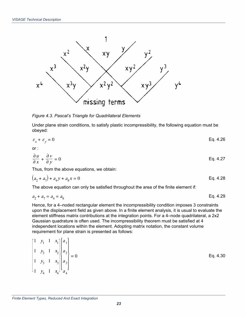
Figure 4.3. Pascal’s Triangle for Quadrilateral Elements

Under plane strain conditions, to satisfy plastic incompressibility, the following equation must beobeyed:

εx + εy = 0 Eq. 4.26

or :

∂u∂ x + ∂v

∂ y = 0 Eq. 4.27

Thus, from the above equations, we obtain:

(a2 + a7) + a4y + a8x = 0 Eq. 4.28

The above equation can only be satisfied throughout the area of the finite element if:

a2 + a7 = a4 = a8 Eq. 4.29

Hence, for a 4–noded rectangular element the incompressibility condition imposes 3 constraintsupon the displacement field as given above. In a finite element analysis, it is usual to evaluate theelement stiffness matrix contributions at the integration points. For a 4–node quadrilateral, a 2x2Gaussian quadrature is often used. The incompressibility theorem must be satisfied at 4independent locations within the element. Adopting matrix notation, the constant volumerequirement for plane strain is presented as follows:

1 y1 1 x1

1 y2 1 x2

1 y3 1 x3

1 y4 1 x4

{a 1

a 2

a 3

a 4

} = 0 Eq. 4.30



where (x1,y1) ... (x4,y4) are the co–ordinates of the numerical integration points, which satisfyequation [4].In contrast to this, if the one–point integration rule is employed to evaluate the stiffness matrix of atypical 4–node quadrilateral element, plastic incompressibility will be satisfied at that particularpoint and thus only one constraint is imposed, which is:

a2 + a7 + a4y1 + a8x1 = 0 Eq. 4.31

where (x1,y1) are the co–ordinates of the particular integration point. In the first case, when threeconstraints are imposed in the problem, ’exact’ integration applies, while in the second, ’reduced’integration applies. In both cases, incompressibility is satisfied at the particular integration point(s).Similarly, under axisymmetric conditions the incompressibility theorem becomes:

εr + εz + εθ = 0

∂u∂ r + ∂u

∂ z + ur = 0

Eq. 4.32

Under axisymmetric conditions, the number of constraints per element is four.It is possible to indicate whether the 4–node rectangular element is suitable for predicting collapseloads under plane strain and/or axisymmetric conditions.From equation 4.1 (p.16), the sum of internal degrees of freedom per one 4–node quadrilateral is2π. From equation 4.29 (p.23), the incompressibility theorem imposes 3 constraints in termsof ’exact’ integration and from equation 4.31 (p.24) only one constraint is imposed by ’reduced’integration. The ’incompressibility ratio’ becomes 2/3 when ’exact’ integration is used and 2when ’reduced’ integration is applied. In this case, the 4–node isoparametric rectangular element istheoretically suitable for predicting collapse loads using ’reduced’ integration and unsuitableusing ’exact’ integration. Similar conclusions will apply, if axisymmetric conditions are considered.In Table 4.1 (p.25) and Table 4.2 (p.25) compressibility ratios are evaluated for a number ofdifferent element types assuming ’exact’ integration. The interesting feature these tables is that,under axisymmetric conditions, only the 15–node triangle is capable of predicting collapse loads.These tables is not valid for ’reduced’ integration; the ratio (degrees of freedom)/(constraints) perelement is dependent in this case on the number of integration points selected to carry out theintegration. Thus, for an 8–node rectangular element, if ’reduced’ integration is applied,an ’incompressibility ratio’ of 3/2 will be obtained. As this is greater than unity, it will also make thisparticular element suitable for predicting collapse loads.The main difference between ’exact’ and ’reduced’ integration is that in the former case,incompressibility is satisfied throughout the element area, while in the latter case, it will only besatisfied at the integration points. The number of integration points will increase as the finiteelement mesh is refined. Plastic incompressibility is now satisfied at a greater number of pointswithin the mesh and under such conditions improved collapse loads will therefore be obtainedusing ’reduced’ integration schemes.Successively refining the mesh will yield more accurate solutions for collapse. The rate ofconvergence of the finite element method is dependent on the mesh densities employed in theprimary analysis. Engineering judgement is now required to identify areas where high stressgradients are likely to occur. Once the initial mesh has been defined a simple ’doubling’ scheme



may be adopted in successive analyses, where one element is divided into four. Provided thecompressibility ratio for the element type used in the analysis has been established to be greaterthan or equal to unity, convergence is guaranteed.

Note: Convergence rates can also be improved by increasing the order of the ’shape functions’.

Plane StrainElement Type Degrees of

Freedom perElement

Integration Rule Constraintsper Element

Ratio Degreesof Freedom ÷Constraints

Suitable

* 3–noded constantstrain triangle

1 1–point 1 1 Yes

* 6–noded linearstrain triangle

4 3–point 3 4/3 Yes

10–noded quadraticstrain triangle

9 6–point 6 3/2 Yes

12–noded cubicstrain triangle

16 12–point 10 8/5 Yes

*4–noded quad 2 2x2 3 2/3 No*8–noded quad 6 3x3 6 1 Yes12–noded quad 10 4x4 10 1 Yes17–noded quad 16 5x5 14 8/7 Yes

Table 4.1: Suitability of plane strain elements for predicting collapse loads accurately (after Sloan& Randolph, 1982)

Note: All results for rectangular quadrilaterals and straight–sided triangles.

Note: The number of constraints per element shown are minima for quadrilateral and triangularelements of arbitrary shape.

Note: * Row entries after Nagtegaal, Parks and Rice.

Note: Integration rules for triangles from Laursen and Gellert.

AxisymmetricElement Type Degrees of

Freedom perElement

Integration Rule Constraintsper Element

Ratio Degreesof Freedom ÷Constraints

Suitable



Axisymmetric* 3–noded constant

strain triangle1 3–point 3 1/3 No

* 6–noded linearstrain triangle

4 6–point 6 2/3 No

10–noded quadraticstrain triangle

9 12–point 10 9/10 No

12–noded cubicstrain triangle

16 16–point 15 16/15 Yes

*4–noded quad 2 3x3 5 2/5 No*8–noded quad 6 3x3 9 2/3 No12–noded quad 10 4x4 13 10/13 No17–noded quad 16 5x5 19 16/19 No

Table 4.2: Suitability of axisymmetric elements for predicting collapse loads accurately (after Sloan& Randolph, 1982)

Note: All results for rectangular quadrilaterals and straight–sided triangles.

Note: The number of constraints per element shown are minima for quadrilateral and triangularelements of arbitrary shape.

Note: * Row entries after Nagtegaal, Parks and Rice.

Note: Integration rules for triangles from Laursen and Gellert.



5Finite Element Modelling Of

Plasticity Within VISAGE

5.1 IntroductionWhen an increment of stress is applied to a material, two types of strain may occur; one is elasticand reversible, the other is plastic and irreversible. Based on St. Venant’s theorem, the principalaxes of the increments of plastic strain, should coincide with the principal axes of stress and not ofstress increments. This behaviour contrasts sharply with the behaviour of elastic materials. Herethe principal axes of the increments of strain, coincide with the principal axes of stress incrementsand not of stress. Thus, the basic nature of plastic strain is quite different from elastic strain. Soilsand rocks behave like an elastic material at low stress levels and like a plastic material at highstress levels. Hence, when a soil/rock stress–strain condition is modelled it should definitely takeinto account the plastic nature of the strain at high stresses.Various computational procedures, utilising the finite element method, have been usedsuccessfully for elasto–plastic problems. The first approach is that in which the stress–strainrelationship in every load increment is adjusted to take plastic deformations into account. With aproperly specified elasto–plastic matrix, this incremental elasticity approach can successfully treatideal, as well as hardening plasticity. In this approach, referred to as the ’initial stress’ process,increments of strains, even in ideal plasticity, prescribe the stress system uniquely; the reverse isnot true for ideal plasticity. An adjustment process is then derived in this case, in which initialstresses are redistributed elastically through the structure.The second approach falls into the ’initial strain’ family of processes. In this, during an increment ofloading, the increase of plastic strain is computed and treated as an initial strain, for which theelastic stress distribution is adjusted. The ’visco–plastic’ approach is the most important of this typeof process.

5.2 Physical DeterminationIn the ’visco–plastic’ approach, it is assumed that the only ’instantaneous’ strains which can beproduced by stresses, are elastic. A time–dependent strain is added and its rate, depends on theamount by which some function of the stresses, exceeds a ’yield’ value.


Finite Element Modelling Of Plasticity Within VISAGE 27

To illustrate the situation conceptually, a uniaxial model shown below, is introduced. In this modelthe plastic component can only become active if σ>Y, in which σ is the total actual ’stress’ appliedand Y is the ’yield’ value, defined by the ’yield criterion’. On instantaneous load application, onlyelastic straining of the spring takes place. The excess σ–Y, is taken by the dashpot. This results insome strain, which is time dependent. In a typical model like this, different modifications can bemade, to represent more complex material behaviour. For example, the ’yield’ value Y, can easilybecome strain dependent and also the dashpot and spring characteristics can easily be madenon–linear. This simple uniaxial conceptual situation can be generalised to a multiaxial case, byplacing more than one ’visco–plastic’ models in series and/or parallel.

Figure 5.1. Basic 1–Dimensional Elastic–Visco–Plastic Model

This ’visco–plastic’ model can easily be degenerated to an ’initial stress’ model, simply by omittingthe dashpot component. In this manner, a multiaxial situation can be produced by placing a seriesof springs in series. Thus, there is a fundamental difference between the two models: the totalstress of the visco–plastic model can exceed the ’yield’ value instantaneously, by any desiredamount. This has been noticed in many experiments.In both models, the excess stresses σ – Y are maintained by a set of body forces, which are inequilibrium with the initial system. At this stage of the computation, the system of body forces canbe removed, by allowing the structure, which maintains its elastic properties unchanged, to deformfurther, thus adding new stresses and strains to the existing set. Once again, these are likely toexceed the ’yield’ value, therefore, the process has to be repeated. If the process ’converges’, thenfinally, non–linear compatibility and equilibrium conditions will be satisfied.



5.3 Visco–plastic algorithmHaving described the ’visco–plastic’ approach, the next concern is to implement visco–plasticity, ina way that will guarantee compatibility. This compatibility will assure the fact, that safe conclusionsare drawn for the way in which this method satisfies both plasticity and equilibrium.The sequence illustrated below, is independent of the finite element type used in the analysis.Starting from a converged stress and/or strains at each integration point existing in the finiteelement mesh:

{σo} = σxo, σyo, σzo, σxyo, σyzo, σzxoT

Eq. 5.1

{εo} = εxo, εyo, εzo, εxyo, εyzo, εzxoT

Form the stiffness matrix for each finite element, by integrating over its volume, using all thenecessary integration points to satisfy the incompressibility theorem:

KM = ∫ B DTv

B d V Eq. 5.2

where, [B ] is the strain–displacement matrix, resulting at each integration point and [D ] is theelastic stress–strain matrix.Assemble all the element stiffness matrices [KM], into the global stiffness matrix [K].Apply the external force, either in terms of prescribed nodal displacements changes, or byincrementing the external force and calculating the nodal displacements, using some form of anelimination process:

{Δδ} = K −1{ΔP} Eq. 5.3

At each integration point, calculate the strains corresponding to the nodal displacements of thefinite element type on which it lies:{Δϵ} = B {Δδ} Eq. 5.4

Assuming elastic behaviour, calculate the corresponding stresses at each integration point withinthe element:{Δσ} = D {Δε} Eq. 5.5

Add any previous converged stresses to those obtained by the above equation, to evaluate thetotal stresses at each integration point:

{σ} = {σ0} + {Δσ} Eq. 5.6

and from those total stresses, evaluate the stress invariantsUsing a pre–selected failure criterion, evaluate the value of the ’yield function’ in terms of theabove stress invariants:

F = F (J 1, J2, J3, k) Eq. 5.7

where, J1 J2 and J3 are the first, second and third stress invariants respectively and k is a functionof state parameters which are related to hardening/softening parameters.



Consider the sign of equation of F. If F <0 at all integration points, the material behaves elastically.If F ≥ 0 at any integration point, the ’yield criterion’ used in the analysis has been violated; excessstresses, which must be redistributed into neighbouring integration points in the mesh, exist.With the ’yield criterion’ violated, the ’visco–plastic’ approach differs, from other numericaltechniques as mentioned earlier, in the way it iterates to achieve convergence, without violatingequilibrium in the end.

’Visco–plasticity’The ’visco–plastic’ model, shown above, can be generalised to include most behaviour patternsencountered in soils. It is first postulated, that the total strain is a sum of elastic and visco–plasticcomponents. Thus:

{Δε} = {Δε}e + {Δε}v pEq. 5.8

From Figure 5.1 (p.28), it can be seen that when ’yield’ occurs, the rate of movement of thedashpot will be a function of the magnitude of the ’yield’ violation. The general ’visco–plastic’ ratelaw may be written as:

εvp = γ ⋅ f (F ) ⋅ { ∂Q∂ σ } Eq. 5.9

here for real visco–plastic materials:γ is the fluidity parameter of the dashpot,f is a function of the yield criteria F,Q is the visco–plastic potential.When the method is applied to time independent elasto–plastic materials γ = 1.0 and f (F) = F.The method can accommodate both associated and non–associated flow rules. Setting Q= Fmakes the flow rate associated.To ensure no ’visco–plastic’ flow below the ’yield’ limit, it is considered that:

f (F ) = 0 if F < 0 Eq. 5.10

Respectively:

f (F ) = f (F ) if F ≥ 0 Eq. 5.11

if any violation of the ’yield criterion’, at any integration point, has occurred which in turn shouldgive a positive value for the function F, due to an underestimation of the plastic strains that haveoccurred.Instead of accumulating stresses back to the ’yield’ surface, using the plastic stress–strain matrixused by ’initial stress’ methods, ’visco–plasticity’ accumulates the visco–plastic strains at eachtime–step; these are then converted to plastic stresses and finally to body loads. The purpose ofthe time–step within the ’visco–plastic’ approach, as well as its magnitude, will be specified later onin this chapter.At a specific time–step, the visco–plastic strain is given by:



{Δε}vp = ∫ t

t+Δtεvpdt Eq. 5.12

Bearing in mind that, when the time–step is of a small enough value, the strain rate may beassumed to be constant over it and a linear approximation is used:

{Δε}vp = Δt ⋅ εvp Eq. 5.13

The excess stresses are then calculated by:

{Δσ}p = D ⋅ {Δε}vp Eq. 5.14

which are used to obtain a set of bodyloads from equation [21]. These bodyloads are added to thenodal forces at each time–step and the procedure is repeated.In general, the steps below are followed in the ’visco–plastic’ approach between two consecutivetime steps, t and t +Δ t.1. Knowing at time t (iteration number), a nodal redistribution force {ΔP} of the applied force, the

nodal displacements are evaluated, making use of the stiffness matrix of the whole structure,[K], thus:

{Δδ}t = K −1 ⋅ {ΔP}t Eq. 5.15

2. For each integration point, evaluate the total strain increments, making use of the above nodaldisplacements:

{Δε}t = B ⋅ {Δδ}t Eq. 5.16

3. At this step, the ’visco–plastic’ approach is different to other approaches, because the elasticpart of the total strain is estimated to obtain the stresses. Thus:

{Δσ}t = D ⋅ ({Δε}t − {Δε}vpt ) Eq. 5.17

for the first iteration or for any ’unyielded’ integration point, {Δε}vp = 0.4. Add the above stresses to any converged stress at the previous increment:

{σ} = {σo} + {Δσ} Eq. 5.18

5. Convert the stresses into invariants and calculate the ’yield function’ .6. If = 0, proceed to the next integration point; if not, calculate the visco–plastic strain rate:

εvpt = γ ⋅ F t ⋅ { ∂Q

∂ σ }tEq. 5.19

7. Update the visco–platic strain increment as follows:

{Δε}vpt+Δt = {Δε}vp

t + Δt ⋅ εvp⋅t Eq. 5.20

8. Evaluate the body–loads equivalent to the change in visco–plastic strain and then add them tothe external nodal forces:



{ΔP}t+Δt = {ΔP}t + Σ∫ vB T D (Δt ⋅ εvp

t )dV Eq. 5.21

9. Return to step 1 and repeat the process, until convergence is achieved. If not, failure of the soilstructure is supposed to have occurred.

Once convergence has been achieved the displacements, stresses and strains are updated for thenext load increment.This process is shown for the problem of a uniaxially loaded bar below.

Figure 5.2. Application of the Visco–Plastic Algorithm

5.4 Convergence CriterionAs already mentioned, the ’visco–plastic’ approach must satisfy non–linear compatibility andequilibrium conditions, iterating in the manner described above. It is therefore necessary toestablish some rules for these iterative procedures: this will ensure accuracy for termination.Otherwise, the repetition of the calculations might continue for an indefinite number of cycles.There are several possibilities, but an important feature of the whole process, is that it must notallow cumulative errors. Thus, one or more convergence criteria must be employed within thenumerical process. This will take care of the total unbalanced force at every load increment and atevery stage of iteration. The purpose of these convergence criteria will be to measure thesatisfaction of the equilibrium equation. Some of these criteria can be used jointly or separately.



Convergence criteria used in VISAGE are :Maximum of displacement changes.Value of yield function F.Maximum of plastic energies.The displacement criteria is

max (Δdt+Δt − Δ d t)max (Δ d t+Δt)

< tol (dimensionless)

where

Δ d t+Δt is the displacement from the current iteration

Δ d t is the displacement from the previous iteration

If convergence on yield function is implemented then the value of the yield criteria F is usedF < tol ( not dimensionless )for all gauss points.The energy criteria is

max (Et+Δt − Et)max (Et+Δt)

< tol (dimensionless)

where E is the plastic energy.For each of these convergence criteria tol is a tolerance specified ’a priori’.However, the influence of any convergence criterion incorporated in any numerical approach, mustbe closely examined, so that its influence on the end result will be minimised.

5.5 Time Step SelectionIt can be seen from the above sequence of equations, that the ’visco–plastic’ approach dependsheavily on the selection of the appropriate time–step *t, which must be incorporated in the analysis.This step–by–step integration of a system of equations in respect to time, obviously leads to afurther approximation, and so adds new errors to the usual space discretisation errors. This is dueto the fact, that {Δε}vp in each time interval is supposed to remain constant, within this small periodof time. This assumes, that any state of stress remains constant during this time increment, while,in reality, it is varying. Thus, an ’a priori’ selection of the time step may cause errors to becomeexcessive and results to be meaningless.Time steps, depend on stresses and viscous properties of the material and may vary from oneelement to another.Assuming an ’explicit’ form of the viscoplastic algorithm this critical time step can be calculated.



The automatic calculation of optimum time steps in viscoplasticity was first addressed by Cormeauwho obtained analytical solutions for a number of failure criteria including Mohr Coulomb. Cormeauextracted analytically, the maximum eigenvalue Ψ from the matrix

A =∂ ε υρ

∂ σ = γ{ ( ∂F∂ σ )T ( ∂Q

∂ σ ) + F ( ∂2 Q∂ σ2 )} Eq. 5.22

and computed the viscoplastic time step

Δtc = 2Ξ / Ψ Eq. 5.23

Ξ is an eigenvalue parameter that categorises the stability of the time stepping computations.Cormeau took Ξ = 1 . Stolle and Higgins, who obtained solutions for the viscoplastic time step forexplicit Euler type elastic viscoplastic time marching schemes, pointed out that Ξ = 1 admits stableoscillatory convergence, whilst Ξ = 0.5 represents an upper bound for non oscillatory stablepredictions.To ensure that non–linear simulations can be performed efficiently, it has been recognised that anautomatic calculation of the viscoplastic time step Δ t is essential.Some explicit expressions for time–step selection are provided from the above equations forsimple yield criteria. These were derived for each ’yield criterion’ from the corresponding ’yieldfunction’. Hence, the critical time–step for a Von–Mises type material is given as:

ΔtVM = 4(1 + v)3Eγ Eq. 5.24

while for Mohr–Coulomb or Tresca material types it becomes:

ΔtMC = 4(1 + v)(1 − 2v)γE(1 − 2v + sin 2φ) Eq. 5.25

As can be seen, when the critical time–step is derived from the above equations and applied inequation [21], the fluidity parameter Υ does not affect the solution, providing it is non–zero.It can be seen that the time step is a function of Young’s modulus. This can have an adverse effecton convergence is there are large variations in Young’s modulus.When an alternative yield criterion to the three above is used in an analysis, the value computed byequation [25] is used and should be factored. For this purpose within VISAGE a multiplying factoris allowed for.When the above time steps are used the time step remains constant throughout the analysis.Alternatively the time step can be calculated automatically by equations [22] and [23]. For thecriteria above this will result in the same critical time steps as given by [24] and [25] for associatedflow. However for all other criteria and non associated flow a varying time step will be calculated asthe equations are dependant on the current state of stress. This will result in a potentially differenttime step at each integration point. As the visco–plastic algorithm is being used to solve elasto–plastic problems ( i.e. no time dependent plastic behaviour ), the time step does not have to be thesame for all the integration points during a particular iteration.



5.6 AcceleratorsIt is often the case that in iterative approaches, such as visco–plasticity’, the rate of convergence tothe correct solution within a load increment, is very slow. The reason for this is usually the stricttolerances described above, necessary to satisfy the kinematic rules imposed by equilibriumand ’yield’.However, the computer run–times become very important and for simple engineering purposes,the finite element method can become an expensive tool.On the other hand, a ’visco–plastic’ approach will generally require a constant number of iterationswhen plasticity occurs, due to time–stepping, if a constant time–step is applied like the ones givenby equations [22] and [23].Thus, modification of the time–step has to take place in a manner, which will speed upconvergence, but also preserve accuracy and stability, at least for those problems for which apreliminary study is made.

Time–step AcceleratorThe selected time–steps in the ’visco–plastic’ approach, described above, depend absolutely onthe ’yield criterion’ used in the analysis to describe the material elasto–plastic behaviour. Thesewere the lowest values which could be used, to preserve the stability and the accuracy of theapproach.If the rate of convergence of the ’visco–plastic’ approach is at least as fast as in the ’initial stress’approach, then the stress corrections due to plasticity for both approaches, must be compatible. Inother words:

{Δσ}vp = {Δσ}p ⇔{Δσ}vp{Δσ}p

= 1 Eq. 5.26

Making use of equations [13], [14] and [15], we obtain:

{Δσ}vp = D ⋅ γ F ⋅ { ∂F∂ σ } ⋅ Δt Eq. 5.27

In the same way, from equations [6] and [15], we obtain:

{Δσ}ep = D { ∂F∂ σ }(A + { ∂F

∂ σ }TD { ∂F

∂ σ })−1⋅ {σ} Eq. 5.28

Inserting equations [25] and [26] into [24] and rearranging, we obtain:

Δt = { ∂F∂ σ }T

D { F∂ σ } −1

⋅ 1γF ⋅ { ∂F

∂ σ }T{σ} Eq. 5.29

Expressing Mohr–Coulomb’s criterion in terms of principal stresses, we obtain:



F = (1 − sin(φ) )2 σ1 −

(1+sin(φ) )2 σ3 − Ccos(φ) = 0

F = μ1σ1 + μ3σ3 − Ccos(φ) = 0Eq. 5.30

where:

μ1 = 1 − sin φ2

μ3 = 1 + sin φ2

thus:

{ ∂F∂ σ } = {μ1 0 μ3} Eq. 5.31

[D] is the plane strain matrix of elasticity and is expressed in terms of the Young’s Modulusand Poisson’s ratio. Inserting all these expressions into equation [29], we obtain:

Δt = 1γF ⋅ (1 + v)(1 − 2v)

E(1 − v) {μ1 0 μ3} D { μ1μ3

} {μ1 0 μ3} Eq. 5.32

but μ1σ1 + μ3σ3 = F + Ccos φ , due to equation [29]; thus, the above equation becomes:

Δt = 2(1 + v)(1 − 2v)γE(1 − 2V + sin2φ ) ⋅ F + Ccos φ

F Eq. 5.33

Considering equation [24], which provides the time–step for a Mohr–Coulomb material type theabove equation becomes:

Δt = 12 ΔtMC ⋅ F + Ccos φ

F Eq. 5.34

Some research must be done on the above expression, bearing in mind that the purpose is only tomake both the iterative approaches described previously, compatible by speeding–up the ’visco–plastic’ approach. So,If F = C cosΦ, then equation [34] becomes:

Δt = 12 ΔtMC ⋅ 2F

F ⇒ Δt = ΔtMC

If F > C cosΦ, then equation [34] becomes:

F + Ccos φF ≤ 2 ⇒ Δt = ΔtMC

If F < C cosΦ, then equation [32], using the same notation should be:

Δt ≥ ΔtMC Eq. 5.35

For this particular case a higher time–step value can be employed. If C = 0 kN/m2, then equation[32] computes a time–step identical to that given by equation [23].



The magnitude of the ratio Δt / ΔtMC , should be found by a trial and error method for each problemwhere it is applied.Pande found that this ratio lies between unity and two.This accelerator should always be used in the context of continuum mechanics.

Aitken’s AcceleratorIn this paragraph, the application of a variation of the Aitken accelerator method, for non–linearproblems, is described.This approach computes an improved estimate of the solution, based on the previous threesuccessive estimates and the process is frequently repeated. Significant savings in solution timewere achieved by Chow and Kay (1984). They applied this method to both static and transientproblems, but did not show any comparisons between results obtained by this and the standardmethod.

Aitken’s δ2 acceleration has been proposed to accelerate the convergence of iterative processes.In the original method, great care has to be exercised when the solution is accelerated.Acceleration at the wrong time, may lead to divergence or worse, give a solution which is in grosserror.Jennings (1977) proposed a variation of the Aitken acceleration method, which has proved to beparticularly useful in geomechanics problems. An improved estimate of displacement vector {Δδ},may be determined from:

{Δδ} = {Δδ}(i) + s({Δδ (i) − {Δδ}(i−1)}) Eq. 5.36

where:

s ={Δδ}(i−1) − {Δδ}(i)

{Δδ}(i−2) − 2{Δδ}(i−1) + {Δδ}(i) Eq. 5.37

The relaxation factor, s, is a scalar and is determined from three successive estimates of the vector{Δδ}.The above equations are used at the beginning of every 3k+1 (where k=1,2,3...) iteration, to givean improved estimate of the vector {Δδ} based on the previous three successive estimates (i.e.{Δδ}(3k–2), {Δδ}(3k–1), {Δδ}(3k)), until convergence of the solution is achieved.

Alternatively, instead of estimating the displacement vector, the out of balance forces – thebodyforces – can be used within the above equations. Equations [35] and [36] are implemented inthe software for the bodyloads.Accelerators should only be used in the context of continuum mechanics. If jointed rock behaviouris modelled they should be avoided.



6Invariant Yield Criteria

Given a state of stress (total or effective) at any integration (gauss) point

{σ} = σx, σy, σz, σxy, σyz, σzxT

Eq. 6.1

then the stress can be written in terms of invariants, independent of the coordinate system used.A convenient choice for these invariants is first principal invariant (I1) of σ and the second and thirdprincipal invariants (J2, J3) of the deviatoric stress, defined as

I1 = Tr(σ) = (σ1 + σ2 + σ3)J2 = 12 s : s = 1

6 (σ1 − σ2)2 + (σ2 − σ3)2 + (σ3 − σ1)2

J3 = det (s) = s1s2s3

where s = σ −I13 I is the deviatoric stress tensor and I is the identity matrix .

Eq. 6.2

Related quantities are (p, J, θ) or (p, q, θ)Mean stress :

p = 13 I1 Eq. 6.3

Equivalent stress :

J = J2 or q = 3 J 2 Eq. 6.4

Lode angle :

θ = tan-1 13 (2 (σ2 − σ3)

(σ1 − σ3) − 1) − 30 ° ≤ θ ≤ 30 ° Eq. 6.5

where σ1, σ2, σ3 are the principal stresses. These stress invariants can be interpreted as shownbelow. The value of p is a measure of the distance along the space diagonal of the current


Invariant Yield Criteria 38

deviatoric plane. J provides a measure of distance from the space diagonal in the deviatoric planeand θ defines the orientation of the stress state within this plane.

Figure 6.1. Invariants in principal stress space

The yield function F is defined as a function of stress and state parameters {k} which are related tohardening/softening parameters:F = F ({σ}, {k}) Eq. 6.6

and the plastic potential function is of a similar form

Q = Q({σ}, {m}) Eq. 6.7

where {m} are again state parameters, which are never used, as only derivatives of Q with respectto stress components are needed.If Q = F then the flow rule is said to be associated. If Q ≠ F then the flow rule is said to non–associated.

6.1 Mohr–Coulomb CriteriaThe yield and potential functions are given by :

F = p sinφ + J (cosθ − sinθ sin φ3 ) − c cos φ Eq. 6.8

where c is the cohesion and φ is the friction angle. The flow rule Q is given by the same equationbut with the friction angle φ replaced by the dilation angle ψ.Hardening/softening is accounted for in the cohesion which is a function of deviatoric plastic strain:

c = cο + H Eεvpd Eq. 6.9



where co is the initial cohesion, H is the hardening/softening parameter, E is the Young’s modulusand εvp d is the equivalent plastic strain:

εvpd =

2.0 εx2 + εy

2 + εz2 + εxy

2 + εyz2 + εzx

2

3.0

1/2Eq. 6.10

Below is shown the relationship between yield and potential surfaces in p–J space.

Figure 6.2. Yield and plastic potential functions

g(Θ) or F and gpp(Θ) or Q are functions of the Lode angle and the friction and dilation anglerespectively.

6.2 Critical State CriteriaThe Critical State model is modelled on the modified Cam Clay model. This is given by an ellipse inthe p–J space and the formulation assumes a Mohr – Coulomb hexagon for yield surface in thedeviatoric plane.The equation of the yield surface is then given by

F = 3.0J 2 + M 2p(p + 2.0pc)

where M = 3.0sin φ3.0cos θ − sin φ sin θ

pc = pcoe χ ϵvp, χ =(1 + eo)(λ − κ)

Eq. 6.11

where φ is the friction angle, χ is the hardening/softening parameter and εvp is the volumetricplastic strain. Also eo is the initial voids ratio, λ is the slope of the virgin consolidation line and κ theslope of the swelling line. p co is the initial radius of the Cam Clay ellipse.

The projection of the yield surface onto the J–p plane and the volumetric behaviour are shownbelow. This shows how the model can simulate both hardening and softening. The flow potential Qis associated and is also given by equation 6.11 (p.40).



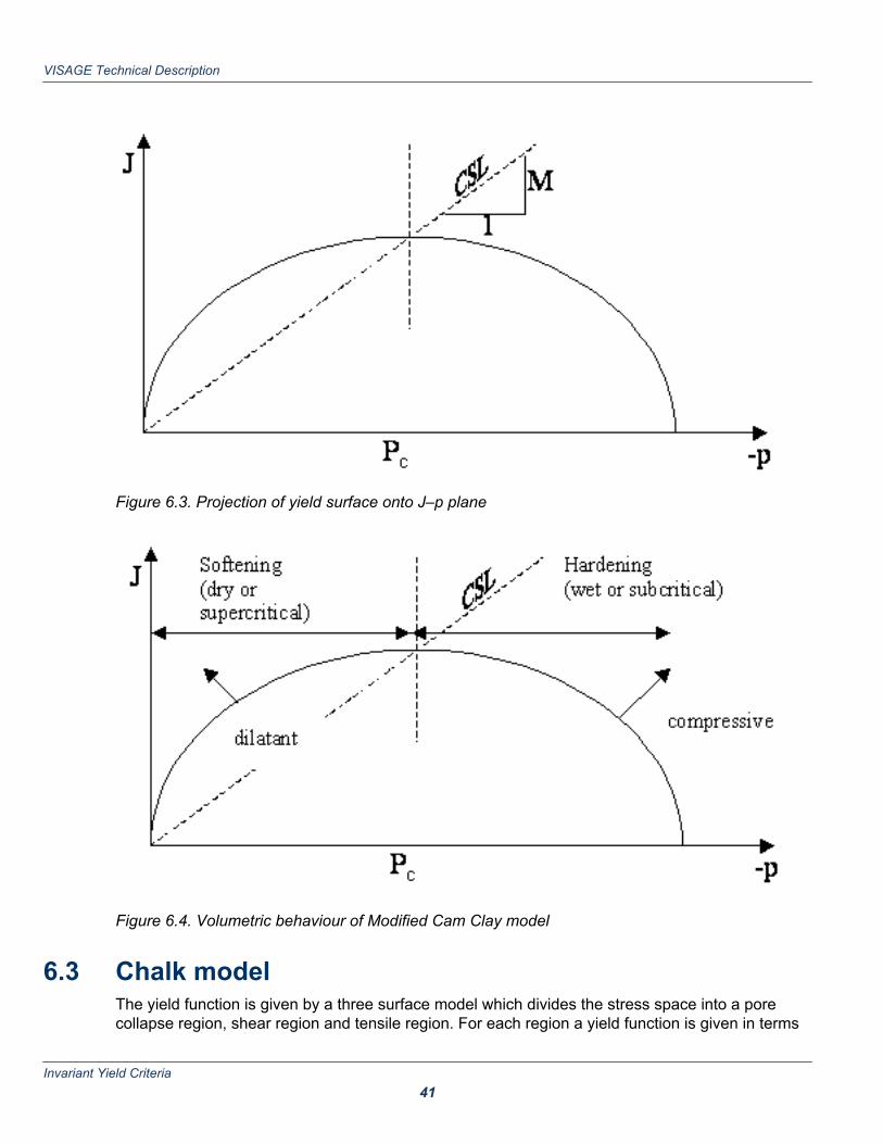
Figure 6.3. Projection of yield surface onto J–p plane

Figure 6.4. Volumetric behaviour of Modified Cam Clay model

6.3 Chalk modelThe yield function is given by a three surface model which divides the stress space into a porecollapse region, shear region and tensile region. For each region a yield function is given in terms



of the three–dimensional stress invariants mean stress p, equivalent stress q and Lode angle θwhich are functions of the stress invariants.The pore collapse failure surface is defined by an elliptical cap surface

Fc = q 2 − (Y ο − a )2 1 − ( (p − Rpmax )(R − 1)pmax

)2

Eq. 6.12

which has an associated flow rule and is assumed to have volumetric strain hardening defined by

dpmax =pmax (1 + eο )

Γ d εvp Eq. 6.13

The shear failure surface is given by the hyperbolic surface

Fs = q − Y ο + a 2 + G(θ)η f (p − Rpmax ) 2

Y ο = qο + a 2 + G(θ)η f Rpmax2

G(θ) = G(θ, k)

η f = 6sin( ϕ)(3 − sin(ϕ))

Eq. 6.14

and is assumed fixed and non–hardening but to have a non–associated flow rule. The plasticpotential being the same as the failure surface with ηf replaced with ηg. G(Θ) accounts for thevariation in the third stress invariant and is given by

G(θ) =c1cos θ + c2(c3 + c4)

c2 + c4c1 = 2(1 − k 2)c2 = (k − 2)2

c3 = (5k − 4)k

c4 = 2c1cos2 θ

Eq. 6.15

The tensile surface is also hyperbolic and given by

Ft = q 2 − qο (ηο pt + qο ) 1 −ηο (p − pt)2

pt(ηο pt + qο )ηο

= −(G(θ)η f )2Rpmax

α 2 + G(θ)η f R pmax2

pt =ηο σt

2

2σ t ηο + qο

Eq. 6.16



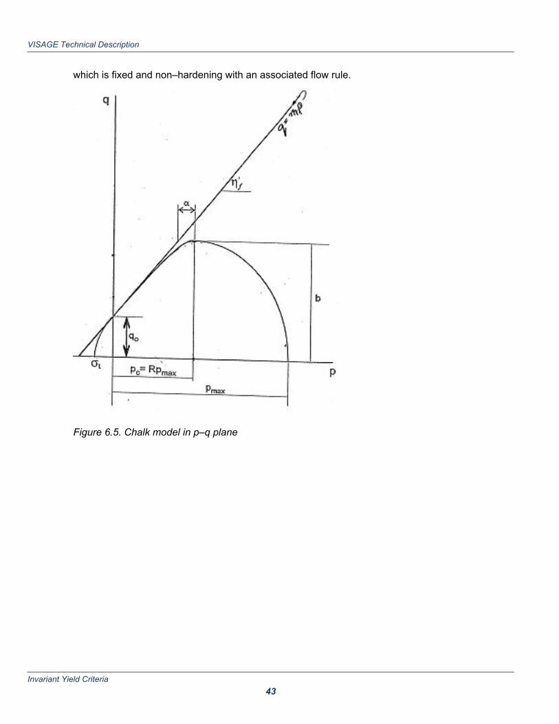
which is fixed and non–hardening with an associated flow rule.

Figure 6.5. Chalk model in p–q plane



Figure 6.6. Chalk model in deviatoric plane

6.4 Modified Drucker–Prager modelThe failure surface is described by the classic Drucker–Prager criterion for unconsolidated material

F (σ) = q + Ap = 0 Eq. 6.17

where again :

p = σkk / 3 , q = 32 sijsij , sij = σij − p δij Eq. 6.18

The parameter A in equation (16) defines the maximum friction coefficient of the material. Thisparameter is kept constant.The plastic yield function is obtained by introducing a scalar valued hardening function η, so that:

F (σ, η) = q + η ⋅ Ap = 0, 0 ≤ η ≤ 1 Eq. 6.19

The plastic hardening is described by a function of the generalized deviatoric plastic strain:



η = η0 + (1 − η0) e pB + e p

Eq. 6.20

e p = ∫0

t( 23 eij

peijp)1/2

d τ Eq. 6.21

where:

eijp = εij

p −εv

p

3 δij

The effective stress space is divided into two zones as shown below, a plastic compressibility zoneand a dilation zone. The transition from compressibility to dilation is defined by the line:

F (σ) = q − ηcAp = 0 Eq. 6.22

The following plastic potential is used for the non–associated flow rule:

Q(σ) = q − ηc A p ln ( pp0

) Eq. 6.23

Figure 6.7. Description of implemented constitutive model



6.5 CRITICAL STATE MODEL WITH HVSORLEV SURFACEThe failure surface is described by the Critical State model with an expanding cap to model thecompaction due to pore collapse on the so called wet side. Shear failure is modeled using aHvorslev rupture surface, on the dry side, with a standard tensile failure criterion in tensile zones.The potential surface is the same as the yield surface.The Critical State model is governed by an ellipse on the wet side in space with a Mohr Coulombhexagon describing failure in the deviatoric plane. The Critical State yield surface is provided bythe equation

Fc = q 2 + M 2p(p + 2.0pc) = 0

with

M = 3sin φ3cos θ − sin φcos θ

Eq. 6.24

pc is the radius of the expanding cap given by

pc = pciexp (ϰ ϵvp) Eq. 6.25

where εvp is the volumetric strain and pci is the initial radius of the ellipse. The hardening parameteris defined as

ϰ = (1 + e)λ − κ Eq. 6.26

where e is the voids ratio, given by

e = Γ + (λ − κ)ln 2r − ln pc0 + κlnpc0p

Eq. 6.27

As shown λ is the slope of the virgin consolidation line, κ is the slope of the swelling line and Γ isthe specific solid volume when p = 1. The eccentricity parameter r is taken here to have unit value.Under such circumstances the parameter pc0 is the outer diameter of the ellipse as shown.

The Hvorslev rupture surface is given by the yield criteria

Fs = q − mh p − (M − mh )pc = 0 Eq. 6.28

mh is the gradient of the rupture surface as shown below.



Figure 6.8. Schematic showing Normal Consolidation Line (NCL) together with the Critical StateLine (CSL).

Figure 6.9. Tensile failure surface together with Hvorslev rupture surface, Critical State Line andCritical State failure surface with cap



7Jointed Rock and theMultilaminate Model

7.1 IntroductionThe mechanical behaviour of rock masses is often dominated by the properties and spatiallocations of the discontinuities within such masses. When inter–connected, these discontinuitiesdefine individual rock blocks that can become unstable under certain conditions.Excavations and other mechanical or thermal fluid pressure loading processes applied to rockmasses which may contain discontinuities, can produce changes in stress and/or geometry thatinitiate instability.Discrete zones of weakness, like faults or joints can be modelled by individual elements andsuitable material properties. However if the number of joints in a rock mass is very large so thatmodelling becomes impossible, a different model has to be used. Here we describe constitutivelaws which can be used to model such jointed rock masses.The methodology adopted within VISAGE is that of an ’equivalent’ material. In the followingsections a brief description of the constitutive behaviour of this material will be given.

7.2 ’Equivalent’ MaterialAnalyses assuming an ’equivalent’ material behaviour, rely on the assumptions that thediscontinuities occur in regular sets and that the spacing between members within each set ismuch smaller than the dominant dimension describing the external geometry of the particularproblem. Economy in analysis is a compensating factor for the restrictions imposed by theseassumptions.The ’equivalent’ material concept is based on developing a constitutive law for a material that willbehave in the same way as the rock mass, with its discrete sets of discontinuities. This means thatthe ’equivalent’ material is formulated by ’smearing out’ the influence of each discontinuity setthroughout the respective volumes that they occupy.


Jointed Rock and the Multilaminate Model 48

The theory behind this ’equivalent’ material is based on the visco–plastic algorithm and is capablein accounting for both the deformational and failure behaviour in the intact rock material and thesets of discontinuities.The theory is first developed by considering the rheological units that represent each component inthe rock mass, i.e. intact rock material and the sets of discontinuities. The representation of therock mass by series connection of these units leads to the formulation of the general equationsdescribing the behaviour of the ’equivalent’ material.

7.3 Constitutive Equations of Rock MassA rock mass is considered to consist of rock material intersected by sets of planar discontinuitiesThe members in each set of discontinuities are assumed to be parallel, continuous and evenlyspaced at dimensions that are small in comparison with the critical dimension of the rock mass,e.g. height of a slope, the diameter of a tunnel and width of a foundation.The definition of local axes with respect to the reference axes is necessary in order to provide linksbetween the global axes and the local axes of the discontinuities of the rock mass.Local sets of co–ordinates are required to describe:The elastic anisotropy of the rock materialThe orientation of each set of discontinuities.Global co–ordinates are used to formulate the overall problem of the mechanical response of therock mass in terms of the ’equivalent’ material. Appropriate transformations are required totransform matrices, such as the stiffness matrix and vectors, such as stresses and strains, fromlocal to global co–ordinates and vice versa.Discontinuity planes are so named because they permit relative displacements to develop. For aset of discontinuity planes, these relative movements, when divided by the spacing between theplanes can be interpreted as strains. The total global strain vector for the rock mass is given bysumming the global strain vector for the rock material with those for each of the sets ofdiscontinuities. Each set of discontinuities is considered to occupy a negligible volumetricproportion of the rock mass and it is therefore assumed that the same global stress vector will beexperienced by the rock mass and each set of discontinuities.The rock mass is composed of the rock material and sets of discontinuities. In order to enablecomplex modes of response to be modelled and for mathematical convenience each component isrepresented in the analysis by a visco–plastic unit.The analysis of the mechanical behaviour of the rock mass proceeds by developing the constitutiverelations for the ’equivalent’ material whose response considers the interaction of all of theconstituent components, i.e. the ’intact’ rock, the discontinuities with associated sets of interfaces.The rheological analogue of the ’equivalent’ material is illustrated in 7.1 (p.51) and can be seento consist of units connected in series to form a ’string’. Each of the units in a ’string’ is subjected tothe same increment of stress, while the increment of strain for the ’string’ is given as the sum of theincremental strains of the units.It can be seen that the ’string’ in 7.1 (p.51) consists of the ’intact’ rock and all the sets ofdiscontinuities. The series connection ensures that the ’intact’ rock and the sets of discontinuitieswill experience an identical increment of stress and will have increments of strain that are additive.



7.4 Elasticity Matrix Of Jointed Rock MassJoints are attributed with a normal and shear stiffness due to poor contact of joint surfaces,resistance of the joints to closure, friction on the joint walls and compressibility of the infilling gaugematerial. These stiffnesses (k) can be used to derive a complete elasticity matrix of a jointed rockmass [DRM] with multiple joint sets. Assuming that the joints are parallel, with uniform spacing andthat the volumetric space is negligible the ’equivalent’ material model is used. The movement of ajoint under a stress σ is given by σ/ k.Consider a joint plane and define a local co–ordinate axes ( x’,y’,z’) on this plane with z’ normal tothe plane and x’ ,y’ lie within the plane. A compliance matrix s can then be defined which relatesstresses on the plane to relative movements:

{wvu

} =S11 S12 S13

S21 S22 S23

S31 S32 S33

{ σn

τs1

τs2

} Eq. 7.1

It is unlikely that all 9 components of the compliance matrix will be known. Usually only the normalcompliance s11 and a general shear compliance ss will be known. It is assumed that s22 and s33the shear compliances are then equal to ss/√2 and that all off diagonal terms are zero. It may benoted that under these circumstances the compliances are the inverses of the stiffnesses.Assuming a set of parallel joints within a set having a joint frequency f and the same compliance oneach joint then the overall compliance in the global co–ordinate system is

S = f T sT T Eq. 7.2

where T is a transformation matrix form the local joint co–ordinate system to the global system andf is the joint frequency( number of joints per unit length).If there are n sets of joints, then the total compliance (S*) is given by

S * = Σi=1

nf iT isiT i

T Eq. 7.3

and the average strain in the joints by

εJ = S *σ Eq. 7.4

The total strains in the rock mass are the sum of the intact rock strains and the joint strains leadingto a final form for the elasticity matrix of the rock mass [DRM] of

σ = DRM ε

DRM = DI−1 + S * −1 Eq. 7.5

where [DI] is the intact rock elasticity matrix. This is the complete form of the elasticity matrix ofthe ’equivalent’ material. These equations take into account the elastic characteristics of thejoints( through stiffness), the spacing of the joints, orientation of the joints and the elastic



characteristics of the intact rock. Formation of the rock mass elasticity matrix as above leads to ageneral anisotropic elasticity matrix.Alternatively an anisotropic elasticity matrix could be assumed initially. However to obtain the 21independent elastic constants for a general anisotropic material is an extremely difficult task. Theabove formulation allows for an anisotropic elastic stiffness matrix to be calculated from anarbitrary joint fabric.

7.5 Non – linear Behaviour Of Jointed Rock MassThe non–linear behaviour of the jointed rock mass is modelled by the multilaminate theory. Thetheory is formulated in terms of local coordinates and can describe the amount of sliding andopening along a discontinuity plane. The theory is implemented within the framework of visco–plasticity. As for the elastic model the joint sets are assumed to be parallel and continuous and tooccupy a small volume in relation to the total rock mass. Each set of discontinuity planes is givenstrength parameters incorporated within a failure criterion. The model is represented rheologicallyin 7.1 (p.51). It assumes that there are n sets of discontinuities all having the same failurecriteria. The stress acting in each component is the same and the elasticity matrix of the intact rockand joints is all lumped together in the single spring.

Figure 7.1. Rheological model for multilaminate model

The model fits within the framework of visco–plasticity with the following modifications.



At any integration point the stress within the rock mass is given by


Eq. 7.6

which is transformed to normal and shear stresses on a joint plane k

{σ}k = σn, σs kT

Eq. 7.7

Using the normal and shear stresses within a failure criteria the visco–plastic strain rate for a jointset in the global coordinate system is

εvpk = γk ⋅ f (F )k ⋅ { ∂Qk

∂ σk}{ ∂ σk

∂ σ } Eq. 7.8

It is assumed that the intact rock also yields and gives the following visco–plastic strain rate

εvpi = γi ⋅ f (F )i ⋅ { ∂Q i

∂ σ } Eq. 7.9

The total visco–plastic strain rate at an integration point will be the sum of the contributions fromeach joint set and the intact rock

εvp = εvpi + Σ

k=1

nεvp

k Eq. 7.10

this strain rate is used within the visco–plastic algorithm.( See Equation 5.19 (p.31))The total model (elastic and plastic) as described above involves the following :Intact Rock : elastic properties, strength parameters, failure criterion and flow rule.Joint sets : elastic stiffness( Ks ,Kn), orientation, spacing, strength parameters, failure criterion andflow rule.

7.6 Multilaminate model for soilsThe multilaminate model can also be used to model soils (clays,sands). It has the advantages overinvariant models of being able to account for anisotropic behaviour induced by the failure criteria.Also effects of rotation of principal stresses are accounted for.The multilaminate model for jointed rocks described above assumed that the joints within the rockmass and hence anisotropy can be represented by a number of discontinuity planes. If the numberof discontinuity planes approaches infinity then isotropic behaviour is restored. The globalbehaviour is obtained by integrating over all the discontinuities. This is done by the use of asuitable integration rule. The global strain is thus evaluated by summing up shear and normalstrains for each discontinuity in the global co–ordinate system. Conceptually this means that soilsare considered to be composed of discrete particles which are relatively free to move with respectto each other. The contact forces between particles can be split up into normal and tangentialcomponents. The overall deformation of the soil is made up of deformation of individual particlesand relative sliding between them. The inter–particle sliding which is governed by the shearresistance at the contacts between particles makes a major contribution to the overall strain and



this contribution is accounted for in the multilaminate model. Anisotropic behaviour induced byplasticity is captured as depending on the stress path sliding will occur on certain discontinuitiesand others will remain elastic.A numerical integration is required to integrate the local strains on the discontinuity planes. Thenumber, distribution and orientation of these planes are governed by the integration rule. Shownbelow is a general integration rule based on a unit sphere which is used in place of an infinitenumber of planes. The orientation of each plane is represented by direction cosines given inrelation to the global coordinates.

Figure 7.2. Integration planes at an integration point.

Typically 13, 28 or 72 planes are used. Larger numbers of planes require greater computingresources.At each integration point the same yield criteria is used for all discontinuity planes. The stress stateon each plane is transformed into normal and shear stresses. Then for each plane the yield criteriaand plastic potential function are evaluated. Depending on the stress path plastic deformations dueto hardening/softening will take place on certain planes while others will remain elastic. Therefore,plastic flow on various planes automatically leads to directional anisotropy due to the stress path.The multilaminate model can be used with any elasto–plastic model. The two most common arethe Mohr–Coulomb model for sands and Critical State model for clays.



7.7 Joint and Multilaminate Yield CriteriaGiven a state of stress (total or effective) at any integration point


Eq. 7.11

the stress is converted to normal and shear stresses on the joint plane

{σn} = σn, τsT

Eq. 7.12

by

{σn}T = T {σ}T Eq. 7.13

where T is a transformation matrix based on the direction cosines of the normal to the joint plane.The direction cosines are calculated automatically from the joint angles ( dip and dip direction ).The yield function F is defined as a function of stress and state parameters {k} which are related tohardening/softening parameters:

F = F ({σn}, {k}) Eq. 7.14

and the plastic potential function is of a similar form

Q = Q({σn}, {m}) Eq. 7.15

where {m} are again state parameters, which are never used as only derivatives of Q with respectto stress components are needed.If Q = F then the flow rule is said to be associated. If Q ≠ F then the flow rule is said to non–associated.Two yield criteria are available for the joint model. These are a Mohr – Coulomb model andBarton’s failure criteria.Three models are available for the multilaminate model. These are Mohr – Coulomb model,modified Cam Clay critical state model and modified Cam Clay critical state model with Horslevfailure surface and eccentricity.

7.8 Mohr–Coulomb Criteria for JointsThe yield and potential functions are given by :

F1 = σn k=1,n= 0

F2 = | τs | + σntan ∅k − ck k=1,n= 0

Eq. 7.16

and



Q1 = σn − constantk=1,n

= 0

Q2 = | τs | + σntan Ψk − constantk=1,n

= 0Eq. 7.17

where c k is the cohesion, Φk is the friction angle and ψk is the dilation angle of the kth joint set. Theyield function is represented by Mohr–Coulomb failure F2 together with a no tension cut–off F1.

The flow rule Q is given by the same equation but with the friction angle Φ replaced by the dilationangle ψ.Hardening/softening is accounted for in the cohesion which is a function of shear plastic strainvarying linearly from the initial value to a residual cohesion over a given shear plastic strain:

c = co −(co − cR)

τsR τs Eq. 7.18

where c o is the initial cohesion, c R is the residual cohesion at shear strain.

Figure 7.3. Yield and plastic potential functions



Figure 7.4. Hardening/softening function

7.9 Barton’s Criteria for JointsAn alternative criteria based on the Mohr – Coulomb criteria but allowing for variation of c and Φwith normal stress. The failure criteria is based on the empirical formula for the peak strength ofrock joints calculated by Barton and Chaubey. The failure function is given as :

F = | τs | + σntan (JRClog10 ( JCS− σn

) + φr)k=1,n

= 0 Eq. 7.19

whereJRC is the Joint Roughness CoefficientJCS is the Joint Compressive StrengthΦr is the residual friction angle. Below is shown a normalised plot of the criteria.



Figure 7.5. Normalised plot of failure criteria

A non associated potential function is assumed given by

Q = | τs | +σntan λ1

k1− JRC

264σn

2

JCSk=1,n

= 0

λ1 = JRClog10 ( JCS− σn

) + φr

λ2 = λ1 − φr

k1 = 1 − tanλ2tan φr

Eq. 7.20

7.10 Mohr–Coulomb Criteria for Multilaminate ModelThis is the same as the criteria used for the joint rock model except that the change in c forhardening/softening is given by

c = co + HE εvpn Eq. 7.21

7.11 Critical State Criteria for Multilaminate ModelFor each plane the failure criteria is given by

F = | τ | 2 + μ 2σn(σn + 2.0pc) Eq. 7.22

where



μ = tan φ = slope of the critical state line in σn − τ space

pc = pcoe χε vpn

χ =1 + eoλ − k

εvpn = is the normal plastic strain on the plane

Eq. 7.23

The potential surface is associated with Q = F.Shown below is the modified cam clay ellipse in σn – τ space.

Figure 7.6. Modified Cam Clay Yield Surface in σn – τ space

7.12 Critical State Criteria with Horslev failure andeccentricity for Multilaminate ModelThis is the same as the standard modified cam clay model on the wet side of the ellipse. On thedry side the ellipse is replaced with a Horslev surface. Additionally the centre of the ellipse isallowed to be positioned generally along the normal stress axis.The failure criteria on the wet side in given by:

Eq. 7.24



− σn − g1pc ≥ 0.0

Fi = τ 2 + μ12( − σn − g1pc)2 − (μg1pc) = 0

μ = tan φ ′ = slope of the critical state line in σn − τ space

g2 = 2 − g1

μ1 = μg1g2

pc = pc0ex

εnvp

and

pco = initial radius of ellipse

εnvp = plastic normal strain

pc = current radius of ellipse

χ =1 + e0λ − k = hardening parameter

The flow potential is associated.The yield function on the dry side by :

σn − g1pc < 0.0

Fi = | τ | + σntan φ0 = 0

φo = Horslev friction angle

Eq. 7.25

with the flow potential given as below to ensure continuity of the flow potential at the critical stateline.

Qi = | τ | + S2g1pc

( − σ ′n− g1pc)2

− μg1pc = 0

S = dilatancy parameterEq. 7.26



In addition a tension cut–off is incorporated as in the Mohr – Coulomb criteria. The complete yieldfunction is shown below.

Figure 7.7. Complete Yield Surface



8Modelling of Reinforced Rock

8.1 IntroductionThe mechanical behavior of rock masses is often dominated by the properties and spatial locationsof the discontinuities within such masses. When interconnected, these discontinuities defineindividual rock blocks that can become unstable under certain conditions.Excavations and other mechanical or thermal fluid pressure loading processes applied to rockmasses which may contain discontinuities, can produce changes in stress and/or geometry thatinitiate instability. Under these conditions rock bolts and dowels have proved effective techniquesof stabilizing rock masses. The increased stiffness and strength can be estimated on a ’rational’basis through the development of improved mathematical models.However, because of the complex interactions of geometry, stress regimes and mechanicalproperties, the mathematical modelling of rock – reinforcement is a difficult task.The methodology adopted within VISAGE is that of an ’equivalent’ material. In the followingsections a brief description of the constitutive behavior of this material will be given.

8.2 ’Equivalent’ MaterialAnalyses assuming an ’equivalent’ material behavior, rely on the assumptions that thediscontinuities and the reinforcements occur in regular sets and that the spacing betweenmembers within each set is much smaller than the dominant dimension describing the externalgeometry of the particular problem. Economy in analysis is a compensating factor for therestrictions imposed by these assumptions.The ’equivalent’ material concept is based on developing a constitutive law for a material that willbehave in the same way as the reinforced rock mass, with its discrete sets of discontinuities andreinforcements. This means that the ’equivalent’ material is formulated by ’smearing out’ theinfluence of each discontinuity set and each reinforcement set throughout the respective volumesthat they occupy.The theory behind this ’equivalent’ material is based on the visco–plastic algorithm that wasdescribed earlier, in Section 15.5, and is capable in accounting for both the deformational andfailure behavior of the rock material, the sets of discontinuities and the sets of reinforcements.


Modelling of Reinforced Rock 61

The theory is first developed by considering the rheological units that represent each component inthe reinforced rock mass, i.e. rock material, sets of discontinuities and sets of reinforcement. Therepresentation of the reinforced rock mass by parallel/series connection of these units leads to theformulation of the general equations describing the behavior of the ’equivalent’ material.The definition of the global axes with respect to the reference axes is necessary in order to providelinks between the global axes and the local axes of the components of the reinforced mass.

8.3 Constitutive Equations of Reinforced MassA rock mass is considered to consist of rock material intersected by sets of planar discontinuities,while the insertion of linear sets of reinforcements creates the reinforced rock mass. The membersin each set of discontinuities or reinforcement are assumed to be parallel, continuous and evenlyspaced at dimensions that are small in comparison with the critical dimension of the rock mass,e.g. height of a slope, the diameter of a tunnel and width of a foundation.Local sets of coordinates are required to describe:• The elastic anisotropy of the rock material• The orientation of each set of discontinuities.• The direction of each set of reinforcement.Global coordinates are used to formulate the overall problem of the mechanical response of thereinforced rock mass in terms of the ’equivalent’ material. Appropriate transformations are requiredto transform matrices, such as the stiffness matrix and vectors, such as stresses and strains, fromlocal to global coordinates and vice versa.Discontinuity planes are so named because they permit relative displacements to develop. For aset of discontinuity planes, these relative movements, when divided by the spacing between theplanes can be interpreted as strains. The total global strain vector for the rock mass is given bysumming the global strain vector for the rock material with those for each of the sets ofdiscontinuities. Each set of discontinuities is considered to occupy a negligible volumetricproportion of the rock mass and it is therefore assumed that the same global stress vector will beexperienced by the rock mass and each set of discontinuities.Reinforcement sets can be considered in the categories of active and passive. At any stage in asequence of loading or unloading/excavation, active reinforcement sets are those in which there isa manually induced change in the stress level. In effect, active reinforcement can be considered asa component of the loading and in order to exert this effect, it must be ungrouted. Passivereinforcement may be grouted or ungrouted and forms an integral part of the rock mass. Frictionbolts are considered as special cases of grouted reinforcement.The total global stress vector for the reinforced rock mass will be shared between the rock massand each of the sets of reinforcement. It will be given by the sum of the products of the volumetricproportions and global stress vectors for the rock mass and for each of the sets of reinforcement.The reinforced rock mass is composed of several components, viz. rock material and sets ofdiscontinuities and reinforcements with interfaces. In order to enable complex modes of responseto be modelled and for mathematical convenience each component is represented in the analysisby a visco–plastic unit. These units have been extensively described in Section 15.5.



The analysis of the mechanical behavior of the reinforced rock mass proceeds by developing theconstitutive relations for the ’equivalent’ material whose response considers the interaction of all ofthe constituent components, i.e. the ’intact’ rock, the discontinuities and the reinforcement withassociated sets of interfaces. The rheological analogue of the ’equivalent’ material is illustrated inFigure 15 14 and can be seen to consist of units connected in series to form ’strings’ that are inturn connected in parallel. Each of the units in a ’string’ is subjected to the same increment ofstress, while the increment of strain for the ’string’ is given as the sum of the incremental strains ofthe units. Because of the parallel connection, the increment of strain for each ’string’ will beidentical and will equal that for the ’equivalent’ material. The incremental load on the ’equivalent’material will be shared by all the ’strings’ with the fraction taken in each ’string’ being given by theproduct of its volumetric proportion and its increment of stress.It can be seen that the first ’string’ of units in Figure 15 14 consists of the ’intact’ rock and all thesets of discontinuities. The series connection ensures that the ’intact’ rock and the sets ofdiscontinuities will experience an identical increment of stress and will have increments of strainthat are additive. Each of the subsequent ’strings’ consists of a set of reinforcement and anassociated interface set. The stress increment in one of these ’strings’ is experienced by both thereinforcement and the interface. The increments of strain of the reinforcement and its interface areadditive and in sum equals each of the strain increments in all other ’strings’.A simpler version of this rheological model has been implemented into VISAGE in that nointerfaces are incorporated directly and failure of a reinforcement set is said to have been achievedat the yield stress of the interface.The mathematical description of the above rheological model has not been included as it can befound in the References and Bibliography.



Figure 8.1. Rheological Model of Reinforced Mass



9Equation Solvers

9.1 IntroductionDuring a finite element analysis the solution of the following set of linear equations:

K {Δd} = {ΔP} Eq. 9.1

is required. [K] is the global assembled stiffness matrix and is of size n by n where n is the totalnumber of unknowns in the problem.Matrix [K] can contain many zeros and in addition be banded about the diagonal. In general [K] canbe asymmetric but depending on the problem [K] may also be symmetric. Distribution of the zerosand extent of the band are dependent on the mesh numbering of the problem. Symmetry of theglobal matrix depends on the material models being used.Two methods are used to solve the set of simultaneous equations , a direct method based onGaussian elimination or an iterative technique.

9.2 Solution TechniquesThere are three main solution techniques used within VISAGE for the solution of the finite elementequations. They are the in–core skyline, the out–of–core skyline and the iterative solvers.In the skyline solutions the central non–zero diagonal part of the stiffness matrix defining thestructure is stored. This is then solved as a whole or in parts. If it is solved in parts, then an out ofcore solver is said to be in use. The out of core method is used for larger skyline problems.It is particularly important for the banded solution to keep the width of the band as low as possibleas the solution time will be proportional to the square of the bandwidth. The semi–bandwidth will bedefined by the maximum number difference in any element plus one multiplied by the number ofdegrees of freedom being used. To achieve the optimum bandwidth, the REORDER interface isprovided as part of The VISAGE System.In some hardware platforms, such as PC's, computer memory limitations usually prevent thesolution of large problems and suitable algorithms have to be developed which will allow thememory bounds to be exceeded by means of reading and writing to and from disks or tapes.


Equation Solvers 65

The solution of problems by The VISAGE System is based on various bandwidth solvers, capableof administrating problem requirements which exceed such memory bounds.For static analyses the direct equation solver both in core and out of core is based on a skylinesolver, which is based on Choleski elimination.The iterative solvers are independent of element and/or nodal ordering sequence. The stiffnessmatrix must be positive definite and, for large problems, provides an effective solver from both theCPU and memory management points of view.There is a threshold above which the iterative solvers are much faster than the skyline solvers.Below this threshold, the skyline provides a faster solution as it requires only one inversion of theglobal stiffness matrix. This threshold value is dependent on the number of elements, elementtypes and number of dimensions. It also depends on the memory available on the machine.As a general rule it is always good practice to number the structure for optimum bandwidth andfrontwidth. This will enhance the ability of The VISAGE System to solve problems that demandsubstantial memory stacks, although this is not important for the iterative solver.

9.3 VISAGE solver optionsTypes of solver

in–core symmetric skyline solvercontrolled out–of–core symmetric skyline solverautomatic out–of–core skyline symmetric solveriterative symmetric solveriterative asymmetric solverin – core asymmetric skyline solverout of core iterative symmetric solverimproved memory management iterative solverpreconditioned improved iterative solver (AMG)

Table 9.1:


Equation Solvers 66

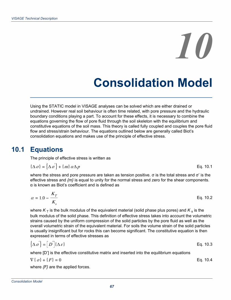
10Consolidation Model

Using the STATIC model in VISAGE analyses can be solved which are either drained orundrained. However real soil behaviour is often time related, with pore pressure and the hydraulicboundary conditions playing a part. To account for these effects, it is necessary to combine theequations governing the flow of pore fluid through the soil skeleton with the equilibrium andconstitutive equations of the soil mass. This theory is called fully coupled and couples the pore fluidflow and stress/strain behaviour. The equations outlined below are generally called Biot’sconsolidation equations and makes use of the principle of effective stress.

10.1 EquationsThe principle of effective stress is written as

{Δσ} = {Δσ ′} + {m}α Δp Eq. 10.1

where the stress and pore pressure are taken as tension positive. σ is the total stress and σ’ is theeffective stress and {m} is equal to unity for the normal stress and zero for the shear components.α is known as Biot’s coefficient and is defined as

α = 1.0 −KTKs

Eq. 10.2

where K T is the bulk modulus of the equivalent material (solid phase plus pores) and K s is thebulk modulus of the solid phase. This definition of effective stress takes into account the volumetricstrains caused by the uniform compression of the solid particles by the pore fluid as well as theoverall volumetric strain of the equivalent material. For soils the volume strain of the solid particlesis usually insignificant but for rocks this can become significant. The constitutive equation is thenexpressed in terms of effective stresses as

{Δσ ′} = D ′ {Δε} Eq. 10.3

where [D’] is the effective constitutive matrix and inserted into the equilibrium equations

∇{σ} + {F } = 0 Eq. 10.4

where {F} are the applied forces.


Consolidation Model 67

Flow of pore fluid flow through the porous medium is defined by Darcy’s law{v} = − k {∇h }

h = pγ f

+ {iG} Eq. 10.5

where h is the hydraulic head, {iG} is a gravity vector and [k] is the permeability matrix. γf is the unitweight of the pore fluid.The equation of continuity and compressibility for the fluid is given as :

∇T {v} − Q = fluid accumulation terms Eq. 10.6

Terms relating to fluid accumulation are :

rate of change of total volumetric strain ∂ ϵv∂ t = {m}T ∂ ϵ

∂ trate of change of the solid volume due to pressure changes

(1 − n)Ks

∂ p∂ t

rate of change of fluid density n

Kw

∂ p∂ t

and change of solid volume due to effective stress changes − 13K s

{m}T ∂{σ ′}∂ t

where substituting for ∂{σ ′}∂ t from the constitutive equation gives

− 13K s

{m}T D ′( ∂{ε}∂ t + {m}

3K s

∂ p∂ t )

where n is the porosity and K w is the bulk modulus of the fluid.

The continuity equation is then given by

∇T {v} − Q = ({m}T −{m}T D ′

3K s) ∂ ε∂ t + (1 − n)

Ks+ n

Kw− 1

(3K s)2 {m}T D ′{m} ∂ p∂ t Eq. 10.7

where Q represents any fluid flow (sources or sinks) and the terms on the RHS represent any fluidaccumulation due to fluid and matrix compressibility.In equation [7] the term is equal to 3K T for an isotropic material and equation [7] can now bewritten as



∇T {v} − Q = {m}T a ∂ ε∂ t + (1 − n)

Ks+ n

Kw−

KT

(Ks)2∂ p∂ t Eq. 10.8

Introducing Skempton’s coefficient β for an undrained test as

β =

1KT

− 1Ks

n 1Kw

− 1Ks

+ 1KT

− 1KS

Eq. 10.9

it can be shown that the final term in equation [8] can be rewritten as

η = α (1 − αβ)β

1KT

Eq. 10.10

which is termed the storage capacity and is equal to 1 over the Biot Modulus.Using a suitable finite element method such as the Galerkin method, minimum potential energy orprinciple of virtual work the equations of equilibrium and continuity defined above become :

K {d{u} / dt} + C {dp / dt} = {dF / dt} Eq. 10.11

where

K = ∫Ω

B T D ′BdΩ

C = ∫Ω

B T α N dΩ

{F } = ∫Ω

N T dbdΩ + ∫ΓN T d tdΓ

Eq. 10.12

and

KP {p} + C T {d{u} / dt} + CP {dp / dt} = {Q} + {G} Eq. 10.13

where



KP = ∫Ω

(∇ N )T k (∇ N )γ f

dΩ

C T = ∫Ω

N T αBdΩ

CP = ∫Ω

N T η N dΩ

{G} = ∫Ω

(∇ N )T k (iG)dΩ

Eq. 10.14

Equations [11] and [13] can be written as a set of ordinary differential equations:

0 00 KP { {u}

p } +K C

C T CPddt {{u}

p } = { {dF / dt}{Q} + {G}} Eq. 10.15

To solve the above equation a time marching scheme is required. Assuming a linear variation intime the equation becomes:

K CC T − KP θΔt t − CP { {u}

p }k+1

=K C

C T KP (1 − θ)Δt t − CP { {u}p }

k

+{ {dF }({Q} + {G})Δt t

} Eq. 10.16

where Δtk is the consolidation time step at step (increment) k and Θ is a time step parameterranging form 0.0 to 1.0.

10.2 General notesThe unknowns {d} are solved at each node in the finite element mesh.The unknowns p are solved only at corner nodes in the finite element mesh.For linear elements the same shape functions are used for both sets of unknowns.For quadratic elements linear shape functions are used for the pore pressure freedoms andquadratic shape functions for the displacement freedoms. This avoids any in consistency in thevariation of stress and pore pressure across an element, as both are now linear.In addition to the usual material properties the following are required:Biot’s coeffeicient – αSkempton’s coefficient – βUnit weight of fluid – γf

Permeability over unit weight of fluid – [k]/ γf

All elastic and plastic properties should be in terms of effective stress parameters.



Boundary conditions :The natural hydraulic boundary condition at any node on the boundary is for no flow i.e. animpermeable boundary.Prescribed pore pressures are given by the total accumulated value for any time step.Pore fluid flows can be either at a node or over a surface of an element. For surface flowrates theflow is converted into equivalent nodal flows internally within the software.Prescribed displacements are given by the accumulated value for any time step.Stress loads either point forces or distributed loads are total loads.Consolidation time increments need to be specified plus the time stepping parameter Θ.By default no units are assumed within the software so all material properties, loads and time stepsneed to be in consistent units.



11Fracture/Fault Permeability

Enhancement/Reduction

11.1 Permeability EnhancementThe parameter Alpha as defined below is used to determine permeability enhancement duringsimulations.

ΔK osKos

= α ( εnVm max

) when εn < Vm max

ΔK osKos

= α when εn ≥ V m max

where εn is the strain normal to the fracture, Kos is the original permeability along the fault directionand ΔKos is the enhancement along the fault.

• The default value of Alpha is 99.0.


Fracture/Fault Permeability Enhancement/Reduction 72

Figure 11.1. Sketch of the variation of permeability enhancement factor with εn

11.2 Permeability ReductionAalpha as defined below is used to determine permeability reductions during simulationstransverse to direction of the fracture.

ΔKonKon

= 0 ε s ≤ Vm max

ΔK onKon

= − A α ( εsVm max

− 1) V m max < εs < 2V m max

ΔK onKon

= − A α ε s ≥ 2V m max

where εs is the maximum shear strain in the transverse direction of the fracture, Δ K on ispermeability reduction normal to the fault. K on is the original permeability normal to the fault.



Figure 11.2. Sketch of the variation permeability reduction factor with εs

InitialisationIn a 2D problem with one single square cell for the reservoir:

Figure 11.3.

the initial permeabilities in the model are:PERMX = PERMY = 2 milliDarcyCreate the following embedding (new cells are also square and of the same dimensions as thereservoir cell) :



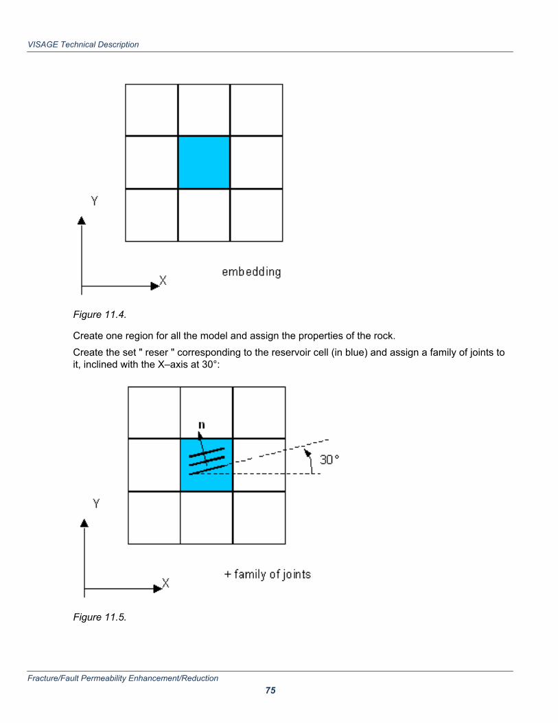
Figure 11.4.

Create one region for all the model and assign the properties of the rock.Create the set " reser " corresponding to the reservoir cell (in blue) and assign a family of joints toit, inclined with the X–axis at 30°:

Figure 11.5.



As Z–direction is the vertical direction, the dip angle would be 90°, and if we suppose that Y–direction is the North direction, then the dip direction would be 30°.

Note: What are in this case the values of the original permeability k0s along the fault and thepermeability k0n normal to the fault ?

As the global permeability is isotropic when these values are calculated in the jointdirection they will also be 2 millidarcys in both the normal and shear directions.EnhancementConsider only an enhancement of the permeability along the fault by choosing the followingparameters for the family of joints:α = 1, Aα = 0, Vm max 0Run the simulation (suppose that there is an injecting well in the center of the reservoir, whichconstitutes the loading). Imagine that, due to the variation of the pressure induced by the injection,the plastic strain normal to the family of joints εn becomes bigger than the Vm max parameter (εn ≥Vm max).

According to the graph, the actual permeability ks along the joint should be increased to twice theinitial permeability k0s along the joint with kn remaining constant.

Note: Then, what are the new values for PERMX and PERMY that will be actualised in for the nexttime step?

The kn remains constant and the ks is doubled ’ these values are then transformed back tothe global co–ordinates x and y producing a full permeability tensor with off diagonal termswhich is now the global permeability. This will produce an anisotropy in the globalpermeabilities.The maths goes like this –Initial permeability –Global : Kx = 2 ; Ky = 2 ; Kxy = 0.0Joints : Kn = 2 ; Ks = 2Get enhancement Ekn = 0 Eks = 2 (increase in joint directions) i.e. Kn =2 Ks = 4Transform enhancement to global co–ords.Ekx = 1.5Eky = 0.5Ekxy = 0.8660 ( off diagonal term )Get new global permsNkx = kx + Ekx = 2.0 + 1.5 = 3.5Nky = kx + Eky = 2.0 + 0.5 = 2.5Nkxy = kxy + Ekxy = 0.0 + 0.8660 = 0.8660



12Additional Topics

An important feature of the VISAGE system is the capability to restart an analysis and apply forexample new loading conditions. This chapter describes restart facilities and also explains how toperform parametric studies, such as changing the convergence tolerance by direct editing of theMII input file for VISAGE.As explained in the VISAGE Reference Manual, data input is simplified in the VISAGE system bythe use of keywords. Further direct control is available with the use of environmental variables.Thus for example it is possible to change the solver type from iterative to exact i, without having toedit the input MII file directly. Environmental variables offer a powerful means of controlling theruntime environment.Step–by–step procedures are described here covering:• Restarts

• restarting a non–linear analysis that has not converged• using a restart to apply new loads• using restarts in mining operations

• Parametric Studies• changing non–linear properties• incrementing the loading• varying the convergence tolerance

• Use of environmental variables• changing iterative solver tolerances• performing an elastic analysis

Note: The VISAGE system file structure is described in the VISAGE Reference Manual.


Additional Topics 77

12.1 RestartsThis section identifies a number of situations where the restart facility is required to complete ananalysis:• restarting a non–linear analysis that has not converged• using restarts to apply new loadsIn all these situations the user follows similar procedures to generate and read modeln.TOM restartfiles. The following sub–keywords can be found under the *RESTART and *HEADER keywords.To this end the following sub–keywords are available for restarts :

Keyword Parameter Description#Sreadrestart sreadrestart switch for reading modeln.TOM#readrestartfile modelname specify rootname for reading modeln.TOM file#Swriterestart swriterestart switch for writing modeln.TOM#writerestartfile modelname specify rootname for writing modeln.TOM file#saccumulatedisp saccumulate switch to accumulate displacements#niterations niteration maximum number of non–linear iterations

Table 12.1: Sub–keywords Available for Restart Analyses

Note: Switch values are off by default [0]. Set equal to 1 to activate.

Note: You can only perform a restart analysis if swriterestart = 1 in the original analysis. Undersuch circumstances a restart modeln.TOM file will be generated.

Restarting a Nonlinear Analysis that has not Converged

DescriptionThis type of situation will occur if the maximum number of permitted iterations set by the parameterniterations has been exceeded during the course of an analysis. For highly CPU intensive analysesit is advisable to set niterations=100 [default 1000]. If the analysis has not converged this approachwill enable the results to be post–processed and checked to ensure that the analysis is proceedingsatisfactorily. In this way modelling errors can be detected at an early stage ensuring that thecomputing time can be used efficiently. Under such circumstances restart the analysis withniterations = 500.

Note: If the maximum number of iterations has been exceeded and no restart file was requested,then repeat the analysis increasing the niterations parameter and set swriterestart =1.

Note: If required use #writerestartfile to specify a rootname for the modeln.TOM file.



What to doTo perform a restart analysis the user can edit the VISAGE MII input file.

Editing the MII file• Locate the sub–keyword #Niterations in the *HEADER section.• Increase the parameter niterations on this sub–keyword.• If the sub–keyword cannot be found then by default niterations = 1000 has been used in the

analysis. Under such circumstances insert:

#Niterations 1500

Table 12.2:

• Type in the *RESTART keyword the read restart sub–keyword:

#Sreadrestart 1

Table 12.3:

• To generate a file for a second restart leave:

#Swriterestart 1

Table 12.4:

• Repeat the procedure for running VISAGE.

Using a Restart to Apply New Loads

DescriptionIt is often required to employ restarts to study the effect of secondary loading on a structure afterprimary loads have been applied. The procedures are straightforward and the user merely has touse the standard sub–keywords for writing and reading restart files that have already been outlinedin this chapter.

What to do• Use PreProcessor to modify the loads as shown in Table 6 2. Applied loads are classified in the

VISAGE system as either total or incremental, depending on the module being used.

Module LoadingIncremental Total

STATIC Not consolidation For consolidation

Table 12.5: Loading Classification

• If for example a linear static analysis is restarted and the old loads are left in the MII file, theseloads will then be reapplied together with any new loads.



• In consolidation analyses the old loads must be left in the MII to preserve equilibrium uponrestart.

Note: Remember to set #saccumulatedisp = 1 if it is required to accumulate displacements.

Using Restarts in Mining Operations

DescriptionThe use of restarts is fundamental when modelling mining operations where load distributions areconstantly changing during excavation and backfilling sequences. It is constructive to consider theapplication of the restart facility to this type of operation.

What to doConsider three stages in a mining operation modelled by the mii files:

Stress initialization 1tun01.miiExcavation stage 1tun02.miiBackfilling stage 1tun03.mii

Table 12.6:

Set up the problem for a static analysis in 1tun01.mii with #sgravity =1.

copy 1tun01.mii to 1tun02.miicopy 1tun01.mii to 1tun03.miichange the modelname in 1tun02.mii to 1tun02change the modelname in 1tun03.mii to 1tun03

• Stress initialisation–1tun01.mii• set #sgravity = 1• under *RESTART input the following :

#swriterestart1#swriterestartfile1tun02

• Excavation• 1tun02.mii• keep #sgravity = 1• set the Young’s modulus for regions to be excavated to 1.0E–10 (to make them inactive)• under *RESTART input the following :

#sreadrestart1#sreadrestartfile 1tun02#swriterestart1#swriterestartfile 1tun03



• Backfilling• 1tun03.mii• keep #sgravity = 1• set the Young’s modulus for regions to be backfilled to that of the backfilling material. Set

the backfilling material parameters.• under *RESTART input the following :

#sreadrestart1#sreadrestartfile 1tun03#swriterestart1#swriterestartfile 1tun04 is restart file for a possible fourth stage

Note: Remember to set #saccumulatedisp = 1 if it is required to accumulate displacements.

CAUTION: The Young’s Modulus controls the various construction sequences. The unit weightdoes not now have to be reset.

12.2 Parametric StudiesThis section shows how parametric studies may be performed effectively and efficiently. Thesection explains how to• change nonlinear properties• increment the loads• vary the convergence tolerance.

Changing Nonlinear Properties

DescriptionIt is often required in geomechanics to perform parametric studies varying one or more materialproperties in a sequence of analyses to gain an insight into the sensitivity of the numericalsolutions to changes in material data. Typical properties that are often varied include:• the ’cohesion’ parameter for Mohr–Coulomb type materials• the hardening or softening parameter• the yield criterion• the tension cut–off value.

What to doTo change material properties the user can edit the MII file and locate the *MATERIALS[,N]keyword. It is advisable to take copies of the files that are changed.Procedure :



1. Copy the modeln.mat file to a new file.2. Look at the keywords and edit the required material properties.3. Edit the modeln.MII file and change the include file to the new material file.4. Run VISAGE and compare results.

Incrementing the Loads

DescriptionIt is good practice to refine the number of load increments (that are used to apply the appliedloads) and rerun an analysis.

What to doTo refine the number of load steps the user can edit the modeln.mii file and locate the*INCREMENTS keyword. It is advisable to take copies of the files that are changed.Procedure :1. Copy the modeln.MII file to a new new_modeln.MII.2. Edit the new_modeln.MII file.3. Locate the *INCREMENTS keyword and increase the number of load increments by changing

the parameter incs. Modify the print frequency parameter pfreq if required.4. Change the modelname parameter beneath *MODELNAME to new_modelname.5. Save the changes and close the editor.6. Repeat the procedures for running VISAGE etc.

Varying the Convergence Tolerance

DescriptionIn nonlinear analyses it is important to reduce the convergence tolerance to ensure that the resultshave converged.

What to doTo reduce the tolerance the user can edit the modeln.mii file and locate the*VISCOPLASTICMETHOD keyword and change the parameter toler o. Editing of the MII file hasbeen explained earlier in this section.

Note: Remember to change the parameter modelname beneath *MODELNAME if editing a copiedMII file.

Note: For large models it is advisable to initially use a coarse tolerance and then use the restartfacility after checking in Post–Processor that the material data, loads and constraints are correct. It



may be possible to assess at this stage the quality of the mesh and whether a mesh refinement isrequired to pick up any significant stress variations.

12.3 Use of Environmental VariablesEnvironmental variables, as listed in Table 6 3 below, may be used to control the runtimeenvironment. This section describes how to• change iterative solver tolerances• perform an elastic analysiswithout recourse to editing the MII input file directly.

Environmental Variable Input DescriptionVISAGE_STOP_ANALYSIS TRUE/

FALSEstop analysis if modelname and root inputfile name differ

VISAGE_ELASTIC_ANALYSIS TRUE/FALSE

perform an elastic analysis(see*ELASTIC)

VISAGE_NOECHO_ALL TRUE/FALSE

Switch off all selective output controlled by*NOECHO

VISAGE_CGM_MONITOR TRUE/FALSE

Switch off convergence data for iterativesolver

VISAGE_OVERWRITE_FILES TRUE/FALSE

Overwrite files from previous analysis withthe same modelname

VISAGE_SOLVER_METHOD integer Specify solver (see #solver)VISAGE_SOLVER_TOLERANCE real Specify iterative solver toleranceVISAGE_NONLINEAR_TOLERANCE real Specify non–linear convergence toleranceVISAGE_YIELD_VALUE real Specify non–zero elastic value for yield

Table 12.7: Environmental Variable Listing

Changing Iterative Solver Tolerances

DescriptionIt is sometimes useful to change the solver tolerance and assess the convergence of the iterativesolver without having to edit the MII file and change the solver tolerance that is specified using thesub–keyword #vsolvertolerance.

What to doTo change the solver tolerance to 1.0E–07, use the VISAGE Manager Menu Bar to selectExecutable/Variables » View/Update System Variables. Then in the VARIABLE ADJUSMENTCONTROL sections, type

Variable: VISAGE_SOLVER_TOLERANCE



Value: 1.0E–07Upon running VISAGE a warning will be written to the MIO file indicating that the solver tolerancehas been updated.

Perform an Elastic Analysis

DescriptionIt is sometimes useful when performing nonlinear analyses to perform an initial elastic analysis toidentify ’hot spots’, where stress levels are in excess of yield. In this way the effectiveness of themesh can be assessed and decisions made as to whether or not a mesh refinement is required.Use of the environmental variable VISAGE_ELASTIC_ANALYSIS does not now require theinsertion of *ELASTIC in the MII input file.

What to doTo perform an elastic analysis, use the VISAGE Manager Menu Bar to select Executable/Variables » View/Update System Variables. Then in the VARIABLE ADJUSMENT CONTROLsections, type

Variable: VISAGE_ELASTIC_ANALYSISValue: TRUEUpon running VISAGE a warning will be written to the MIO file indicating that an elastic analysiswill now be performed.

Note: It is important to note that all analysis will use these environmental variables, until they areunset.



13References and Bibliography

13.1 ReferencesBATHE, K. J., OZDEMIR, H. and WILSON, E. L. (1974).Static and dynamic geometric and material non–linear analysis.

Report No UC SESM 74–C, February, University of California, Berkeley, California.CHOW, Y. K. and KAY, S. (1984).On the Aitken acceleration method for non–linear problems.

Computers and Structures Vol. 19, No. 5/6 pp. 757–761.HINTON, E., ROCK, T. and ZIENKIEWICZ, O. C. (1976).A note on mass lumping and related processes in the finite element method.

Earthquake Engineering and Structural Dynamics, Vol. 4, pp. 245–249.HOLMAN, J. P. (1986).Heat Transfer

6th Edition.McGraw–Hill, pp. 3.JENNINGS, A. (1977).Matrix computation for engineers and scientists.

John Wiley and Sons UK.KING, P. R. (1994–1995).Informal remarks.

LAURSEN, M. E. and GELLERT, M. (1978).Some criteria for numerically integrated matrices and quadrature formulas for triangles.

Int. J. Num. Meth. Eng., 12, pp. 67–76.LYSMER, J. and KUHLEMEYER, R. L. (1969).


References and Bibliography 85

Finite dynamic model for infinite media.

Journal of the Engineering Mech. Div., ASCE, Vol. 95, No EM4 August, pp. 859–877.NAGTEGAAL, J. C., PARKS, D. M. and RICE, J. R. (1977).On numerically accurate finite element solutions in the fully plastic range.

Comp. Meth. Appl. Mech. Engng, 4, pp. 153–177.PANDE, G. N. (1977).On an accelerator in elasto–viscoplasticity

Internal Report C/R/301/77, University College of Swansea.SLOAN, S. W. and RANDOLPH, M. F. (1982).Numerical prediction of collapse loads using finite element methods.

IJNMAG, Vol. 6, pp. 47–76.SMITH, I. M. and GRIFFITHS, D. V. (1982).Programming the Finite Element Method

2nd Edition, pp. 15–17 and 36–40.John Wiley & Sons Ltd.

13.2 BibliographyThe following bibliography is highly recommended for those who wish to know more about finiteelement techniques, the constitutive models used within VISAGE and the classical theories ofplasticity and visco-plasticity.BEER, G. and WATSON, J. O. (1992).Introduction to Finite and Boundary Element Methods for Engineers.

John Wiley & Sons Ltd.HINTON, E. and OWEN, D. R. J. (1979).An introduction to finite element computations.

Pineridge Press, Swansea, UK.HINTON, E. and OWEN, D. R. J. (1980).Finite Elements in Plasticity: Theory and Practice.

Pineridge Press, Swansea, UK.HOLMAN, J. P. (1986).Heat Transfer

6th Edition.McGraw–Hill.PANDE, G. N., BEER, G. and WILLIAMS, J. R. (1990).Numerical Methods in Rock Mechanics.



John Wileys and Sons.SMITH, I. M. and GRIFFITHS, D. V. (1982).Programming the Finite Element Method.

John Wiley and Sons Ltd.WELTY JAMES, R. (1978)Engineering Heat Transfer

SI Version.John Wiley & Sons, Inc.

13.3 Further ReadingBARTON, N. and CHOUBEY, V. (1977).The Shear Strength of Rock Joints in Theory and Practice.

Rock Mechanics 10, pp. 1–54.GERRARD, C. M. and PANDE, G. N. (1985).Numerical Modelling of Reinforced Jointed Rock Masses I Theory.

Computers and Geotechnics 1, pp. 293–318.GRIFFITHS, D. V. and KOUTSABELOULIS, N. C. (1985).Finite Element Analysis of Vertical Excavations.

Computers and Geomechanics 1, pp. 221–235.HEFFER, K. J. and KOUTSABELOULIS, N. C. (1993).Fracture Scale Effects in Hydrocarbon Reservoirs.

Scale Effects in Rock Masses 93, Pinto da Cunha, 1993, Balkema, Rotterdam.HEFFER, K. J., KOUTSABELOULIS, N. C. and WONG, S. K. (1994).Coupled Geomechanical, Thermal and Fluid Flow Modelling as an Aid to Improving WaterfloodSweep Efficiency.

Eurock ’94, Balkema, Rotterdam.KOUTSABELOULIS, N. C. (1988).Tunnel Design Using the ’Trapdoor’ Problem.

Numerical Methods in Geomechanics (Innsbruck 1988), Swoboda (ed.), Balkema, Rotterdam.KOUTSABELOULIS, N. C. (1993).Numerical Modelling of Soft Reservoir During Fluid Depletion.

Geotechnical Engineering of Hard Soils–Soft Rocks, Anagnostopoulos et al. (eds) 1993 Balkema,Rotterdam.KOUTSABELOULIS, N. C. and GRIFFITHS, D. V. (1989).Numerical Modelling of the Trap Door Problem.



Geotechnique 39, No. 1, pp. 77–89.KOUTSABELOULIS, N. C. and RYLANCE, M. (1990).Acceleration and Deceleration Techniques for ’Viscoplasticity’.

Proceedings of the International Conference on Numerical Methods in Engineering: Theory andApplications/Swansea/7–11 January 1990, Elsevier Applied Science.KOUTSABELOULIS, N. C., HEFFER, K. J. and WONG S. (1994).Numerical Geomechanics in Reservoir Engineering.

Computer Methods and Advances in Geomechanics, Siriwardane & Zaman (eds) 1994 Balkema,Rotterdam.KOUTSABELOULIS, N. C. and RYLANCE, M. (1992).On the Integration of the Multi–Laminate Model for Soils.

Numerical Models in Geomechanics, Pande & Pietruszczak (eds.) 1992 Balkema, Rotterdam.KOUTSABELOULIS, N. C., RYLANCE, M. and EGGINGTON, R. (1991).3–D Finite Element Modelling of the Hope Brook Gold Mine.

Computer Methods and Advances in Geomechanics, Beer, Booker & Carter (eds) 1991 Balkema,Rotterdam.KOUTSABELOULIS, N. C. and GRIFFITHS, D. V. (1989).Dynamic Slope Stability Analysis Using the Finite Element Method.

Computer and Physical Modelling in Geomechanical Engineering, Balassubramaniam et al (eds)1989 Balkema, Rotterdam.NAYLOR, D. J. (1974).Stresses in Nearly Incompressible Materials by Finite Elements with Application to the Calculationof Excess Pore Pressures.

International Journal for Numerical Methods in Engineering Vol. 8, pp. 443–460.PAN, X. D. and HUDSON, J. A. (1988).A Simplified Three Dimensional Hoek–Brown Yield Criterion.

Rock Mechanics and Power Plants, Romana (ed.) 1988 Balkema, Rotterdam.PANDE, G. N. (1985).A Constitutive Model of Rock Joints.

Proceedings of the International Symposium on Fundamentals of Rock Joints/Bjorkliden/15–20September 1985.PANDE, G. N., OWEN, D. R. J. and ZIENKIEWICZ, O. C. (1977).Overlay Models in Time–Dependent Non–Linear Materials Analysis.

Computers and Structures, Vol. 77, pp. 435-443, Pergamon Press.



Documents

VISAGE - Dynpullig.dyndns.org/files/technical_description.pdf · Reservoir Simulator (SDRS), which links the VISAGE System to ECLIPSE. ... The science of geomechanics provides an