Vis. Matching Tone Repr. Op. for High Dyn. Range Scenesradsite.lbl.gov/radiance/papers/lbnl39882/tonemap.pdf · A Visibility Matching Tone Reproduction Operator for High Dynamic Range

A Visibility Matching Tone Reproduction Operatorfor High Dynamic Range Scenes

Gregory Ward Larson†

Building Technologies ProgramEnvironmental Energy Technologies Division

Ernest Orlando Lawrence Berkeley National LaboratoryUniversity of California

1 Cyclotron RoadBerkeley, California 94720

Holly RushmeierIBM T.J. Watson Research Center

Christine Piatko††

National Institute for Standards and Technology

January 15, 1997

This paper is available electronically at:http://radsite.lbl.gov/radiance/papers

Copyright 1997 Regents of the University of Californiasubject to the approval of the Department of Energy

† Author's current address: Silicon Graphics, Inc., Mountain View, CA.†† Author's current address: JHU/APL, Laurel, MD.

LBNL 39882UC 400

A Visibility Matching Tone Reproduction Operatorfor High Dynamic Range Scenes

Gregory Ward LarsonLawrence Berkeley National Laboratory

Holly RushmeierIBM T.J. Watson Research Center

Christine PiatkoNational Institute for Standards and Technology

ABSTRACTWe present a tone reproduction operator that preservesvisibility in high dynamic range scenes. Our methodintroduces a new histogram adjustment technique, based onthe population of local adaptation luminances in a scene.To match subjective viewing experience, the methodincorporates models for human contrast sensitivity, glare,spatial acuity and color sensitivity. We compare our resultsto previous work and present examples of our techniquesapplied to lighting simulation and electronic photography.

Keywords: Shading, Image Manipulation.

1 Introduction

The real world exhibits a wide range of luminance values. The human visual system iscapable of perceiving scenes spanning 5 orders of magnitude, and adapting moregradually to over 9 orders of magnitude. Advanced techniques for producing syntheticimages, such as radiosity and Monte Carlo ray tracing, compute the map of luminancesthat would reach an observer of a real scene. The media used to display these results --either a video display or a print on paper -- cannot reproduce the computed luminances,or span more than a few orders of magnitude. However, the success of realistic imagesynthesis has shown that it is possible to produce images that convey the appearance ofthe simulated scene by mapping to a set of luminances that can be produced by thedisplay medium. This is fundamentally possible because the human eye is sensitive torelative rather than absolute luminance values. However, a robust algorithm forconverting real world luminances to display luminances has yet to be developed.

The conversion from real world to display luminances is known as tone mapping. Tonemapping ideas were originally developed for photography. In photography or video,chemistry or electronics, together with a human actively controlling the scene lightingand the camera, are used to map real world luminances into an acceptable image on a

January 15, 1997 page 1

display medium. In synthetic image generation, our goal is to avoid active control oflighting and camera settings. Furthermore, we hope to improve tone mapping techniquesby having direct numerical control over display values, rather than depending on thephysical limitations of chemistry or electronics.

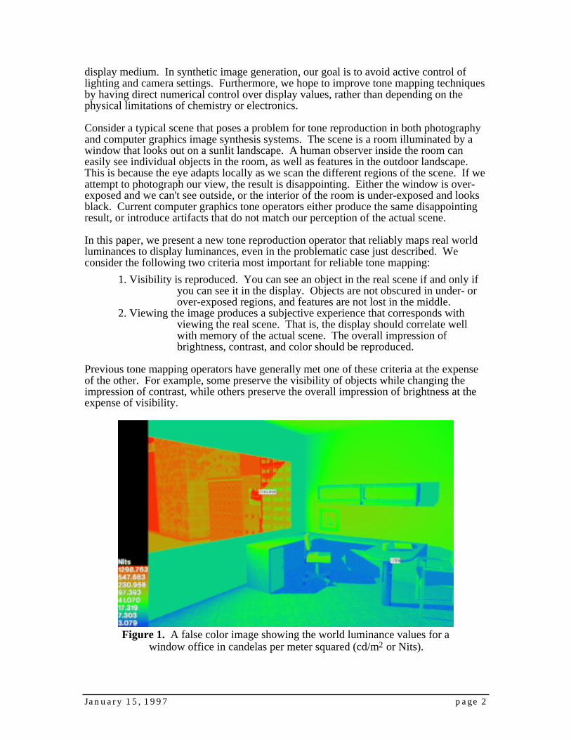
Consider a typical scene that poses a problem for tone reproduction in both photographyand computer graphics image synthesis systems. The scene is a room illuminated by awindow that looks out on a sunlit landscape. A human observer inside the room caneasily see individual objects in the room, as well as features in the outdoor landscape.This is because the eye adapts locally as we scan the different regions of the scene. If weattempt to photograph our view, the result is disappointing. Either the window is over-exposed and we can't see outside, or the interior of the room is under-exposed and looksblack. Current computer graphics tone operators either produce the same disappointingresult, or introduce artifacts that do not match our perception of the actual scene.

In this paper, we present a new tone reproduction operator that reliably maps real worldluminances to display luminances, even in the problematic case just described. Weconsider the following two criteria most important for reliable tone mapping:

1. Visibility is reproduced. You can see an object in the real scene if and only ifyou can see it in the display. Objects are not obscured in under- orover-exposed regions, and features are not lost in the middle.

2. Viewing the image produces a subjective experience that corresponds withviewing the real scene. That is, the display should correlate wellwith memory of the actual scene. The overall impression ofbrightness, contrast, and color should be reproduced.

Previous tone mapping operators have generally met one of these criteria at the expenseof the other. For example, some preserve the visibility of objects while changing theimpression of contrast, while others preserve the overall impression of brightness at theexpense of visibility.

Figure 1. A false color image showing the world luminance values for awindow office in candelas per meter squared (cd/m2 or Nits).


The new tone mapping operator we present addresses our two criteria. We develop amethod of modifying a luminance histogram, discovering clusters of adaptation levelsand efficiently mapping them to display values to preserve local contrast visibility. Wethen use models for glare, color sensitivity and visual acuity to reproduce imperfectionsin human vision that further affect visibility and appearance.

Figure 2. A linear mapping of the luminances in Figure 1 that over-exposes the view through the window.

Figure 3. A linear mapping of the luminances in Figure 1 that under-exposes the view of the interior.


Figure 4. The luminances in Figure 1 mapped to preserve the visibility ofboth indoor and outdoor features using the new tone mapping techniques

described in this paper.

2 Previous Work

The high dynamic range problem was first encountered in computer graphics whenphysically accurate illumination methods were developed for image synthesis in the1980's. (See Glassner [Glassner95] for a comprehensive review.) Previous methods forgenerating images were designed to automatically produce dimensionless values more orless evenly distributed in the range 0 to 1 or 0 to 255, which could be readily mapped to adisplay device. With the advent of radiosity and Monte Carlo path tracing techniques, webegan to compute images in terms of real units with the real dynamic range of physicalillumination. Figure 1 is a false color image showing the magnitude and distribution ofluminance values in a typical indoor scene containing a window to a sunlit exterior. Thegoal of image synthesis is to produce results such as Figure 4, which match ourimpression of what such a scene looks like. Initially though, researchers found that awide range of displayable images could be obtained from the same input luminances --such as the unsatisfactory over- and under-exposed linear reproductions of the image inFigures 2 and 3.

Initial attempts to find a consistent mapping from computed to displayable luminanceswere ad hoc and developed for computational convenience. One approach is to use afunction that collapses the high dynamic range of luminance into a small numericalrange. By taking the cube root of luminance, for example, the range of values is reducedto something that is easily mapped to the display range. This approach generallypreserves visibility of objects, our first criterion for a tone mapping operator. However,condensing the range of values in this way reduces fine detail visibility, and distortsimpressions of brightness and contrast, so it does not fully match visibility or reproducethe subjective appearance required by our second criterion.


A more popular approach is to use an arbitrary linear scaling, either mapping the averageof luminance in the real world to the average of the display, or the maximum non-lightsource luminance to the display maximum. For scenes with a dynamic range similar tothe display device, this is successful. However, linear scaling methods do not maintainvisibility in scenes with high dynamic range, since very bright and very dim values areclipped to fall within the display's limited dynamic range. Furthermore, scenes aremapped the same way regardless of the absolute values of luminance. A sceneilluminated by a search light could be mapped to the same image as a scene illuminatedby a flashlight, losing the overall impression of brightness and so losing the subjectivecorrespondence between viewing the real and display-mapped scenes.

A tone mapping operator proposed by Tumblin and Rushmeier [Tumblin93] concentratedon the problem of preserving the viewer's overall impression of brightness. As the lightlevel that the eye adapts to in a scene changes, the relationship between brightness (thesubjective impression of the viewer) and luminance (the quantity of light in the visiblerange) also changes. Using a brightness function proposed by Stevens and Stevens[Stevens60], they developed an operator that would preserve the overall impression ofbrightness in the image, using one adaptation value for real scene, and another adaptationvalue for the displayed image. Because a single adaptation level is used for the scene,though, preservation of brightness in this case is at the expense of visibility. Areas thatare very bright or dim are clipped, and objects in these areas are obscured.

Ward [Ward91] developed a simpler tone mapping method, designed to preserve featurevisibility. In this method, a non-arbitrary linear scaling factor is found that preserves theimpression of contrast (i.e., the visible changes in luminance) between the real anddisplayed image at a particular fixation point. While visibility is maintained at thisadaptation point, the linear scaling factor still results in the clipping of very high and verylow values, and correct visibility is not maintained throughout the image.

Chiu et al. [Chiu93] addressed this problem of global visibility loss by scaling luminancevalues based on a spatial average of luminances in pixel neighborhoods. Values in brightor dark areas would not be clipped, but scaled according to different values based on theirspatial location. Since the human eye is less sensitive to variations at low spatialfrequencies than high ones, a variable scaling that changes slowly relative to imagefeatures is not immediately visible. However, in a room with a bright source and darkcorners, the method inevitably produces display luminance gradients that are the oppositeof real world gradients. To make a dark region around a bright source, the transition froma dark area in the room to a bright area shows a decrease in brightness rather than anincrease. This is illustrated in Figure 5 which shows a bright source with a dark haloaround it. The dark halo that facilitates rendering the visibility of the bulb disrupts whatshould be a symmetric pattern of light cast by the bulb on the wall behind it. The reversegradient fails to preserve the subjective correspondence between the real room and thedisplayed image.

Inspired by the work of Chiu et al., Schlick [Schlick95] developed an alternative methodthat could compute a spatially varying tone mapping. Schlick's work concentrated onimproving computational efficiency and simplifying parameters, rather than improvingthe subjective correspondence of previous methods.


Figure 5. Dynamic range compression based on a spatially varying scalefactor (from [Chiu93]).

Contrast, brightness and visibility are not the only perceptions that should be maintainedby a tone mapping operator. Nakamae et al. [Nakamae90] and Spencer et al. [Spencer95]have proposed methods to simulate the effects of glare. These methods simulate thescattering in the eye by spreading the effects of a bright source in an image. Ferwerda etal. [Ferwerda96] proposed a method that accounts for changes in spatial acuity and colorsensitivity as a function of light level. Our work is largely inspired by these papers, andwe borrow heavily from Ferwerda et al. in particular. Besides maintaining visibility andthe overall impression of brightness, the effects of glare, spatial acuity and colorsensitivity must be included to fully meet our second criterion for producing a subjectivecorrespondence between the viewer in the real scene and the viewer of the syntheticimage.

A related set of methods for adjusting image contrast and visibility have been developedin the field of image processing for image enhancement (e.g., see Chapter 3 in[Green83]). Perhaps the best known image enhancement technique is histogramequalization. In histogram equalization, the grey levels in an image are redistributedmore evenly to make better use of the range of the display device. Numerousimprovements have been made to simple equalization by incorporating models ofperception. Frei [Frei77] introduced histogram hyperbolization that attempts toredistribute perceived brightness, rather than screen grey levels. Frei approximatedbrightness using the logarithm of luminance. Subsequent researchers such as Mokrane[Mokrane92] have introduced methods that use more sophisticated models of perceivedbrightness and contrast.

The general idea of altering histogram distributions and using perceptual models to guidethese alterations can be applied to tone mapping. However, there are two important


differences between techniques used in image enhancement and techniques for imagesynthesis and real-world tone mapping:

1. In image enhancement, the problem is to correct an image that has alreadybeen distorted by photography or video recording and collapsed intoa limited dynamic range. In our problem, we begin with anundistorted array of real world luminances with a potentially highdynamic range.

2. In image enhancement, the goal is to take an imperfect image and maximizevisibility or contrast. Maintaining subjective correspondence withthe original view of the scene is irrelevant. In our problem, we wantto maintain subjective correspondence. We want to simulatevisibility and contrast, not maximize it. We want to produce visuallyaccurate, not enhanced, images.

3 Overview of the New Method

In constructing a new method for tone mapping, we wish to keep the elements ofprevious methods that have been successful, and overcome the problems.

Consider again the room with a window looking out on a sunlit landscape. Like any highdynamic range scene, luminance levels occur in clusters, as shown in the histogram inFigure 6, rather than being uniformly distributed throughout the dynamic range. Thefailure of any method that uses a single adaptation level is that it maps a large range ofsparsely populated real world luminance levels to a large range of display values. If theeye were sensitive to absolute values of luminance difference, this would be necessary.However, the eye is only sensitive to the fact that there are bright areas and dim areas. Aslong as the bright areas are displayed by higher luminances than the dim areas in the finalimage, the absolute value of the difference in luminance is not important. Exploiting thisaspect of vision, we can close the gap between the display values for high and lowluminance regions, and we have more display luminances to work with to render featurevisibility.

Another failure of using a uniform adaptation level is that the eye rapidly adapts to thelevel of a relatively small angle in the visual field (i.e., about 1°) around the currentfixation point [Moon&Spencer45]. When we look out the window, the eye adapts to thehigh exterior level, and when we look inside, it adapts to the low interior level. Chiu etal. [Chiu93] attempted to account for this using spatially varying scaling factors, but thismethod produces noticeable gradient reversals, as shown in Figure 5.

Rather than adjusting the adaptation level based on spatial location in the image, we willbase our mapping on the population of the luminance adaptation levels in the image. Toidentify clusters of luminance levels and initially map them to display values, we will usethe cumulative distribution of the luminance histogram. More specifically, we will startwith a cumulative distribution based on a logarithmic approximation of brightness fromluminance values.


Figure 6. A histogram of adaptation values from Figure 1 (1° spotluminance averages).

First, we calculate the population of levels from a luminance image of the scene in whicheach pixel represents 1° in the visual field. We make a crude approximation of thebrightness values (i.e., the subjective response) associated with these luminances bytaking the logarithm of luminance. (Note that we will not display logarithmic values, wewill merely use them to obtain a distribution.) We then build a histogram and cumulativedistribution function from these values. Since the brightness values are integrated over asmall solid angle, they are in some sense based on a spatial average, and the resultingmapping will be local to a particular adaptation level. Unlike Chiu's method however, themapping for a particular luminance level will be consistent throughout the image, andwill be order preserving. Specifically, an increase in real scene luminance level willalways be represented by an increase in display luminance. The histogram andcumulative distribution function will allow us to close the gaps of sparsely populatedluminance values and avoid the clipping problems of single adaptation level methods. Byderiving a single, global tone mapping operator from locally averaged adaptation levels,we avoid the reverse gradient artifacts associated with a spatially varying multiplier.


We will use this histogram only as a starting point, and impose restrictions to preserve(rather than maximize) contrast based on models of human perception using ourknowledge of the true luminance values in the scene. Simulations of glare and variationsin spatial acuity and color sensitivity will be added into the model to maintain subjectivecorrespondence and visibility. In the end, we obtain a mapping of real world to displayluminance similar to the one shown in Figure 7.

For our target display, all mapped brightness values below 1 cd/m2 (0 on the vertical axis)or above 100 (2 on the vertical axis) are lost because they are outside the displayablerange. Here we see that the dynamic range between 1.75 and 2.5 has been compressed,yet we don't notice it in the displayed result (Figure 4). Compared to the two linearoperators, our new tone mapping is the only one that can represent the entire scenewithout losing object or detail visibility.

Figure 7. A plot comparing the global brightness mapping functions forFigures 1, 2, and 3, respectively.

In the following section, we illustrate this technique for histogram adjustment based oncontrast sensitivity. After this, we describe models of glare, color sensitivity and visual


acuity that complete our simulation of the measurable and subjective responses of humanvision. Finally, we complete the methods presentation with a summary describing howall the pieces fit together.

4 Histogram Adjustment

In this section, we present a detailed description of our basic tone mapping operator. Webegin with the introduction of symbols and definitions, and a description of the histogramcalculation. We then describe a naive equalization step that partially accomplishes ourgoals, but results in undesirable artifacts. This method is then refined with a linearcontrast ceiling, which is further refined using human contrast sensitivity data.

4.1 Symbols and Definitions

Lw = world luminance (in candelas/meter2)Bw = world brightness, log(Lw)Lwmin = minimum world luminance for sceneLwmax = maximum world luminance for sceneLd = display luminance (in candelas/meter2)Ldmin = minimum display luminance (black level)Ldmax = maximum display luminance (white level)Bde = computed display brightness, log(Ld) [Equation (4)]N = the number of histogram binsT = the total number of adaptation samplesƒ(bi) = frequency count for the histogram bin at bi∆b = the bin step size in log(cd/m2)P(b) = the cumulative distribution function [Equation (2)]log(x) = natural logarithm of xlog10(x) = decimal logarithm of x

4.2 Histogram Calculation

Since we are interested in optimizing the mapping between world adaptation and displayadaptation, we start with a histogram of world adaptation luminances. The eye adapts forthe best view in the fovea, so we compute each luminance over a 1° diameter solid anglecorresponding to a potential foveal fixation point in the scene. We use a logarithmicscale for the histogram to best capture luminance population and subjective response overa wide dynamic range. This requires setting a minimum value as well as a maximum,since the logarithm of zero is -∞. For the minimum value, we use either the minimum 1°spot average, or 10-4 cd/m2 (the lower threshold of human vision), whichever is larger.The maximum value is just the maximum spot average.

We start by filtering our original floating-point image down to a resolution that roughlycorresponds to 1° square pixels. If we are using a linear perspective projection, the pixelson the perimeter will have slightly smaller diameter than the center pixels, but they willstill be within the correct range. The following formula yields the correct resolution for


1° diameter pixels near the center of a linear perspective image:

S = 2 tan(θ/2) / 0.01745 (1)

where:S = width or height in pixelsθ = horizontal or vertical full view angle0.01745 = number of radians in 1°

For example, the view width and height for Figure 4 are 63° and 45° respectively, whichyield a sample image resolution of 70 by 47 pixels. Near the center, the pixels will be 1°square exactly, but near the corners, they will be closer to 0.85° for this wide-angle view.The filter kernel used for averaging will have little influence on our result, so long asevery pixel in the original image is weighted similarly. We employ a simple box filter.

From our reduced image, we compute the logarithms of the floating-point luminancevalues. Here, we assume there is some method for obtaining the absolute luminances ateach spot sample. If the image is uncalibrated, then the corrections for human vision willnot work, although the method may still be used to optimize the visible dynamic range.(We will return to this in the summary.)

The histogram is taken between the minimum and maximum values mentioned earlier inequal-sized bins on a log(luminance) scale. The algorithm is not sensitive to the numberof bins, so long as there are enough to obtain adequate resolution. We use 100 bins in allof our examples. The resulting histogram for Figure 1 is shown in Figure 6.

4.2.1 Cumulative Distribution

The cumulative frequency distribution is defined as:

P(b) =f (bi)

b i < b∑

T (2)

where:T = f (bi)

bi

∑ (i.e., the total number of samples)

Later on, we will also need the derivative of this function. Since the cumulativedistribution is a numerical integration of the histogram, the derivative is simply thehistogram with an appropriate normalization factor. In our method, we approximate acontinuous distribution and derivative by interpolating adjacent values linearly. Thederivative of our function is:

dP(b)

db=

f (b)

T ∆b (3)

where:

∆b =log(Lwmax ) − log( Lwmin)[ ]

N (i.e., the size of each bin)


Figure 8. Rendering of a bathroom model mapped with a linear operator.

4.3 Naive Histogram Equalization

If we wanted all the brightness values to have equal probability in our final displayedimage, we could now perform a straightforward histogram equalization. Although this isnot our goal, it is a good starting point for us. Based on the cumulative frequencydistribution just described, the equalization formula can be stated in terms of brightnessas follows:

Bde = log(Ldmin) + log(Ldmax) − log(Ldmin)[ ]⋅ P(Bw ) (4)

The problem with naive histogram equalization is that it not only compresses dynamicrange (contrast) in regions where there are few samples, it also expands contrast in highlypopulated regions of the histogram. The net effect is to exaggerate contrast in large areasof the displayed image. Take as an example the scene shown in Figure 8. Although wecannot see the region surrounding the lamps due to the clamped linear tone mappingoperator, the image appears to us as more or less normal. Applying the naive histogramequalization, Figure 9 is produced. The tiles in the shower now have a mottledappearance. Because this region of world luminance values is so well represented, naive


histogram equalization spreads it out over a relatively larger portion of the display'sdynamic range, generating superlinear contrast in this region.

Figure 9. Naive histogram equalization allows us to see the area aroundthe light sources but contrast is exaggerated in other areas such as the

shower tiles.

4.4 Histogram Adjustment with a Linear Ceiling

If the contrast being produced is too high, then what is an appropriate contrast forrepresenting image features? The crude answer is that the contrast in any given regionshould not exceed that produced by a linear tone mapping operator, since linear operatorsproduce satisfactory results for scenes with limited dynamic range. We will take thissimple approach first, and later refine our answer based on human contrast sensitivity.

A linear ceiling on the contrast produced by our tone mapping operator can be writtenthus:

dLd

dLw

≤Ld

Lw (5a)


That is, the derivative of the display luminance with respect to the world luminance mustnot exceed the display luminance divided by the world luminance. Since we have anexpression for the display luminance as a function of world luminance for our naivehistogram equalization, we can differentiate the exponentiation of Equation (4) using thechain rule and the derivative from Equation (3) to get the following inequality:

exp( Bde ) ⋅f (Bw )

T∆b⋅log(Ldmax ) − log(Ldmin)

Lw

≤Ld

Lw

(5b)

Since Ld is equal to exp( Bde ) , this reduces to a constant ceiling on ƒ(b):

f (b) ≤T∆b

log( Ldmax ) − log( Ldmin)(5c)

In other words, so long as we make sure no frequency count exceeds this ceiling, ourresulting histogram will not exaggerate contrast. How can we create this modifiedhistogram? We considered both truncating larger counts to this ceiling and redistributingcounts that exceeded the ceiling to other histogram bins. After trying both methods, wefound truncation to be the simplest and most reliable approach. The only complicationintroduced by this technique is that once frequency counts are truncated, T changes,which changes the ceiling. We therefore apply iteration until a tolerance criterion is met,which says that fewer than 2.5% of the original samples exceed the ceiling.1 Ourpseudocode for histogram_ceiling is given below:

boolean function histogram_ceiling()tolerance := 2.5% of histogram totalrepeat {

trimmings := 0compute the new histogram total Tif T < tolerance then

return FALSEforeach histogram bin i do

compute the ceilingif ƒ(bi) > ceiling then {

trimmings += ƒ(bi) - ceilingƒ(bi) := ceiling

}} until trimmings <= tolerancereturn TRUE

This iteration will fail to converge (and the function will return FALSE) if and only if thedynamic range of the output device is already ample for representing the sampleluminances in the original histogram. This is evident from Equation (5c), since ∆b is theworld brightness range over the number of bins:

f (bi ) ≤T

N⋅

log( Lwmax ) − log(Lwmin )[ ]log(Ldmax ) − log(Ldmin )[ ] (5d)

1The tolerance of 2.5% was chosen as an arbitrary small value, and it seems to make little difference eitherto the convergence time or the results.


If the ratio of the world brightness range over the display brightness range is less than one(i.e., our world range fits in our display range), then our frequency ceiling is less than thetotal count over the number of bins. Such a condition will never be met, since a uniformdistribution of samples would still be over the ceiling in every bin. It is easiest to detectthis case at the outset by checking the respective brightness ranges, and applying a simplelinear operator if compression is unnecessary.

We call this method histogram adjustment rather than histogram equalization because thefinal brightness distribution is not equalized. The net result is a mapping of the scene'shigh dynamic range to the display's smaller dynamic range that minimizes visible contrastdistortions, by compressing under-represented regions without expanding over-represented ones.

Figure 10 shows the results of our histogram adjustment algorithm with a linear ceiling.The problems of exaggerated contrast are resolved, and we can still see the full range ofbrightness. A comparison of these tone mapping operators is shown in Figure 11. Thenaive operator is superlinear over a large range, seen as a very steep slope near worldluminances around 100.8.

Figure 10. Histogram adjustment with a linear ceiling on contrastpreserves both lamp visibility and tile appearance.


Figure 11. A comparison of naive histogram equalization with histogramadjustment using a linear contrast ceiling.

The method we have just presented is itself quite useful. We have managed to overcomelimitations in the dynamic range of typical displays without introducing objectionablecontrast compression artifacts in our image. In situations where we want to get a good,natural-looking image without regard to how well a human observer would be able to seein a real environment, this may be an optimal solution. However, if we are concernedwith reproducing both visibility and subjective experience in our displayed image, thenwe must take it a step further and consider the limitations of human vision.

4.5 Histogram Adjustment Based on Human Contrast Sensitivity

Although the human eye is capable of adapting over a very wide dynamic range (on theorder of 109), we do not see equally well at all light levels. As the light grows dim, wehave more and more trouble detecting contrast. The relationship between adaptationluminance and the minimum detectable luminance change is well studied [CIE81]. Forconsistency with earlier work, we use the same detection threshold function used byFerwerda et al. [Ferwerda96]. This function covers sensitivity from the lower limit of


human vision to daylight levels, and accounts for both rod and cone response functions.The piecewise fit is reprinted in Table 1.

log10 of just noticeable difference applicable luminance range

-2.86 log10(La) < -3.94

(0.405 log10(La) + 1.6)2.18 - 2.86 -3.94 ≤ log10(La) < -1.44

log10(La) - 0.395 -1.44 ≤ log10(La) < -0.0184

(0.249 log(La) + 0.65)2.7 - 0.72 -0.0184 ≤ log10(La) < 1.9

log10(La) - 1.255 log10(La) ≥ 1.9Table 1. Piecewise approximation for ∆Lt(La).

We name this combined sensitivity function:

∆Lt(La) = "just noticeable difference" for adaptation level La (6)

Ferwerda et al. did not combine the rod and cone sensitivity functions in this manner,since they used the two ranges for different tone mapping operators. Since we are usingthis function to control the maximum reproduced contrast, we combine them at theircrossover point of 10-0.0184 cd/m2.

To guarantee that our display representation does not exhibit contrast that is morenoticeable than it would be in the actual scene, we constrain the slope of our operator tothe ratio of the two adaptation thresholds for the display and world, respectively. This isthe same technique introduced by Ward [Ward91] and used by Ferwerda et al.[Ferwerda96] to derive a global scale factor. In our case, however, the overall tonemapping operator will not be linear, since the constraint will be met at all potentialadaptation levels, not just a single selected one. The new ceiling can be written as:

dLd

dLw

≤∆Lt(Ld )

∆Lt (Lw )(7a)

As before, we compute the derivative of the histogram equalization function(Equation (4)) to get:

exp( Bde ) ⋅f (Bw )

T∆b⋅log(Ldmax ) − log(Ldmin)

Lw

≤∆Lt (Ld )

∆Lt(Lw )(7b)

However, this time the constraint does not reduce to a constant ceiling for ƒ(b). Wenotice that since Ld equals exp(Bde) and Bde is a function of Lw from Equation (4), our


ceiling is completely defined for a given P(b) and world luminance, Lw:

f (Bw ) ≤∆Lt(Ld )

∆Lt (Lw )⋅

T∆bLw

log(Ldmax) − log(Ldmin)[ ]Ld (7c)

where:Ld = exp(Bde), Bde given in Equation (4)

Once again, we must iterate to a solution, since truncating bin counts will affect T andP(b). We reuse the histogram_ceiling procedure given earlier, replacing the linearcontrast ceiling computation with the above formula.

Figure 12. Our tone mapping operator based on human contrastsensitivity compared to the histogram adjustment with linear ceiling usedin Figure 10. Human contrast sensitivity makes little difference at these

light levels.

Figure 12 shows the same curves for the linear tone mapping and histogram adjustmentwith linear clamping shown before in Figure 11, but with the curve for naive histogram


equalization replaced by our human visibility matching algorithm. We see the twohistogram adjustment curves are very close. In fact, we would have some difficultydifferentiating images mapped with our latest method and histogram adjustment with alinear ceiling. This is because the scene we have chosen has most of its luminance levelsin the same range as our display luminances. Therefore, the ratio between display andworld luminance detection thresholds is close to the ratio of the display and worldadaptation luminances. This is known as Weber's law [Riggs71], and it holds true over awide range of luminances where the eye sees equally well This correspondence makesthe right-hand side of Equations (5b) and (7b) equivalent, and so we should expect thesame result as a linear ceiling.

Figure 13. The brightness map for the bathroom scene with lightsdimmed to 1/100th of their original intensity, where human contrast

sensitivity makes a difference.

To see a contrast sensitivity effect, our world adaptation would have to be very differentfrom our display adaptation. If we reduce the light level in the bathroom by a factor of100, our ability to detect contrast is diminished. This shows up in a relatively largerdetection threshold in the denominator of Equation (7c), which reduces the ceiling for the


frequency counts. The change in the tone mapping operator is plotted in Figure 13 andthe resulting image is shown in Figure 14.

Figure 13 shows that the linear mapping is unaffected, since we just raise the scale factorto achieve an average exposure. Likewise, the histogram adjustment with a linear ceilingmaps the image to the same display range, since its goal is to reproduce linear contrast.However, the ceiling based on human threshold visibility limits contrast over much of thescene, and the resulting image is darker and less visible everywhere except the top of therange, which is actually shown with higher contrast since we now have display range tospare.

Figure 14 is darker and the display contrast is reduced compared to Figure 10. Becausethe tone mapping is based on local adaptation rather than a single global or spot average,threshold visibility is reproduced everywhere in the image, not just around a certain set ofvalues. This criterion is met within the limitations of the display's dynamic range.

Figure 14. The dimmed bathroom scene mapped with the function shownin Figure 13.


5 Human Visual Limitations

We have seen how histogram adjustment matches display contrast visibility to worldvisibility, but we have ignored three important limitations in human vision: glare, colorsensitivity and visual acuity. Glare is caused by bright sources in the visual periphery,which scatter light in the lens of the eye, obscuring foveal vision. Color sensitivity is lostin dark environments, as the light-sensitive rods take over for the color-sensitive conesystem. Visual acuity is also impaired in dark environments, due to the complete loss ofcone response and the quantum nature of light sensation.

In our treatment, we will rely heavily on previous work performed by Moon and Spencer[Moon&Spencer45] and Ferwerda et al. [Ferwerda96], applying it in the context of alocally adapted visibility-matching model.

5.1 Veiling Luminance

Bright glare sources in the periphery reduce contrast visibility because light scattered inthe lens and aqueous humor obscures the fovea; this effect is less noticeable whenlooking directly at a source, since the eye adapts to the high light level. The influence ofglare sources on contrast sensitivity is well studied and documented. We apply the workof Holladay [Holladay26] and Moon and Spencer [Moon&Spencer45], which relates theeffective adaptation luminance to the foveal average and glare source position andilluminance.

In our presentation, we will first compute a low resolution veil image from our fovealsample values. We will then interpolate this veil image to add glare effects to the originalrendering. Finally, we will apply this veil as a correction to the adaptation luminancesused for our contrast, color sensitivity and acuity models.

Moon and Spencer base their formula for adaptation luminance on the effect of individualglare sources measured by Holladay, which they converted to an integral over the entirevisual periphery. The resulting glare formula gives the effective adaptation luminance ata particular fixation for an arbitrary visual field:

La = 0.913Lf +K L( , )

2 cos( )sin( )d d> f

∫∫ (8)

where:La = corrected adaptation luminance (in cd/m2)Lf = the average foveal luminance (in cd/m2)L(θ,φ) = the luminance in the direction (θ,φ)

θf = foveal half angle, approx. 0.00873 radians (0.5°)K = constant measured by Holladay, 0.0096

The constant 0.913 in this formula is the remainder from integrating the second partassuming one luminance everywhere. In other words, the periphery contributes less than9% to the average adaptation luminance, due to the small value Holladay determined forK. If there are no bright sources, this influence can be safely neglected. However, brightsources will significantly affect the adaptation luminance, and should be considered inour model of contrast sensitivity.


To compute the veiling luminance corresponding to a given foveal sample (i.e., fixationpoint), we can convert the integral in Equation (8) to an average over peripheral samplevalues:

Lvi = 0.087 ⋅

Lj cos( i, j )

i, j2

j ≠ i∑

cos( i, j )

i, j2

j ≠i∑

(9)

where:Lvi = veiling luminance for fixation point iLj = foveal luminance for fixation point jθ

i,j= angle between sample i and j (in radians)

Since we must compute this sum over all foveal samples j for each fixation point i, thecalculation can be very time consuming. We therefore reduce our costs by approximatingthe weight expression as:

cos2 ≈

cos

2 − 2cos(10)

Since the angles between our samples are most conveniently available as vector dotproducts, which is the cosine, the above weight computation is quite fast. However, forlarge images (in terms of angular size), the Lvi calculation is still the mostcomputationally expensive step in our method due to the double iteration over i and j.

To simulate the effect of glare on visibility, we simply add the computed veil map to ouroriginal image. Just as it occurs in the eye, the veiling luminance will obscure the visiblecontrast on the display by adding to both the background and the foreground luminance.2This was the original suggestion made by Holladay, who noted that the effect glare hason luminance threshold visibility is equivalent to what one would get by adding theveiling luminance function to the original image [Holladay26]. This is quitestraightforward once we have computed our foveal-sampled veiling image given inEquation (9). At each image pixel, we perform the following calculation:

Lpvk = 0.913Lpk + Lv (k) (11)

where:Lpvk = veiled pixel at image position kLpk = original pixel at image position kLv(k) = interpolated veiling luminance at k

The Lv(k) function is a simple bilinear interpolation on the four closest samples in ourveil image computed in Equation (9). The final image will be lighter around glaresources, and just slightly darker on glare sources (since the veil is effectively beingspread away from bright points). Although we have shown this as a luminancecalculation, we retain color information so that our veil has the same color cast as theresponsible glare source(s).

2The contrast is defined as the ratio of the foreground minus the background over the background, soadding luminance to both foreground and background reduces contrast.


Figure 15 shows our original, fully lit bathroom scene again, this time adding in thecomputed veiling luminance. Contrast visibility is reduced around the lamps, but the veilfalls off rapidly (as 1/θ2) over other parts of the image. If we were to measure theluminance detection threshold at any given image point, the result should correspondclosely to the threshold we would measure at that point in the actual scene.

Figure 15. Our tone reproduction operator for the original bathroomscene with veiling luminance added.

Since glare sources scatter light onto the fovea, they also affect the local adaptation level,and we should consider this in the other parts of our calculation. We therefore apply thecomputed veiling luminances to our foveal samples as a correction before the histogramgeneration and adjustment described in Section 4. We deferred the introduction of thiscorrection factor to simplify our presentation, since in most cases it only weakly affectsthe brightness mapping function.


The correction to local adaptation is the same as Equation (11), but without interpolation,since our veil samples correspond one-to-one:

Lai = 0.913Li + Lvi (12)

where:Lai = adjusted adaptation luminance at fixation point iLi = foveal luminance for fixation point i

We will also employ these Lai adaptation samples for the models of color sensitivity andvisual acuity that follow.

5.2 Color Sensitivity

To simulate the loss of color vision in dark environments, we use the technique presentedby Ferwerda et al. [Ferwerda96] and ramp between a scotopic (grey) response functionand a photopic (color) response function as we move through the mesopic range. Thelower limit of the mesopic range, where cones are just starting to get enough light, isapproximately 0.0056 cd/m2. Below this value, we use the straight scotopic luminance.The upper limit of the mesopic range, where rods are no longer contributing significantlyto vision, is approximately 5.6 cd/m2. Above this value, we use the straight photopicluminance plus color. In between these two world luminances (i.e., within the mesopicrange), our adjusted pixel is a simple interpolation of the two computed output colors,using a linear ramp based on luminance.

Since we do not have a value available for the scotopic luminance at each pixel, we usethe following approximation based on a least squares fit to the colors on the MacbethColorChecker Chart™:

Yscot = Y ⋅ 1.33 ⋅ 1+Y + Z

X

−1.68

(13)

where:Yscot = scotopic luminanceX,Y,Z = photopic color, CIE 2° observer (Y is luminance)

This is a very good approximation to scotopic luminance for most natural colors, and itavoids the need to render another channel. We also have an approximation based onRGB values, but since there is no accepted standard for RGB primaries in computergraphics, this is much less reliable.

Figure 16 shows our dimmed bathroom scene with the human color sensitivity function inplace. Notice there is still some veiling, even with the lights reduced to 1/100th theirnormal level. This is because the relative luminances are still the same, and they scatterin the eye as before. The only difference here is that the eye cannot adapt as well whenthere is so little light, so everything appears dimmer, including the lamps. The colors areclearly visible near the light sources, but gradually less visible in the darker regions.


Figure 16. Our dimmed bathroom scene with tone mapping using humancontrast sensitivity, veiling luminance and mesopic color response.

5.3 Visual Acuity

Besides losing the ability to see contrast and color, the human eye loses its ability toresolve fine detail in dark environments. The relationship between adaptation level andfoveal acuity has been measured in subject studies reported by Shaler [Shaler37]. Atdaylight levels, human visual acuity is very high, about 50 cycles/degree. In the mesopicrange, acuity falls off rapidly from 42 cycles/degree at the top down to 4 cycles/degreenear the bottom. Near the limits of vision, the visual acuity is only about 2 cycles/degree.Shaler's original data is shown in Figure 17 along with the following functional fit:

R(La ) ≈ 17.25arctan(1.4log10(La ) + 0.35) + 25.72 (15)

where:R(La) = visual acuity in cycles/degreeLa = local adaptation luminance (in cd/m2)


Figure 17. Shaler's visual acuity data and our functional fit to it.

In their tone mapping paper, Ferwerda et al. applied a global blurring function based on asingle adaptation level [Ferwerda96]. Since we wish to adjust for acuity changes over awide dynamic range, we must apply our blurring function locally according to the fovealadaptation computed in Equation (12). To do this, we implement a variable-resolutionfilter using an image pyramid and interpolation, which is the mip map introduced byWilliams [Williams83] for texture mapping. The only difference here is that we areworking with real values rather than integers pixels.

At each point in the image, we interpolate the local acuity based on the four closest(veiled) foveal samples and Shaler's data. It is very important to use the foveal data (Lai)and not the original pixel value, since it is the fovea's adaptation that determines acuity.The resulting image will show higher resolution in brighter areas, and lower resolution indarker areas.

Figure 18 shows our dim bathroom scene again, this time applying the variable acuityoperator applied together with all the rest. Since the resolution of the printed image islow, we enlarged two areas for a closer look. The bright area has an average level around


25 cd/m2, corresponding to a visual acuity of about 45 cycles/degree. The dark area hasan average level of around 0.05 cd/m2, corresponding to a visual acuity of about 9cycles/degree.

Figure 18. The dim bathroom scene with variable acuity adjustment. Theinsets show two areas, one light and one dark, and the relative blurring of

the two.

6 Method Summary

We have presented a method for matching the visibility of high dynamic range scenes onconventional displays, accounting for human contrast sensitivity, veiling luminance, colorsensitivity and visual acuity, all in the context of a local adaptation model. However, inpresenting this method in parts, we have not given a clear idea of how the parts areintegrated together into a working program.


The order in which the different processes are executed to produce the final image is ofcritical importance. These are the steps in the order they must be performed:

procedure match_visibility()compute 1° foveal sample imagecompute veil imageadd veil to foveal adaptation imageadd veil to imageblur image locally based on visual acuity functionapply color sensitivity function to imagegenerate histogram of effective adaptation imageadjust histogram to contrast sensitivity functionapply histogram adjustment to imagetranslate CIE results to display RGB valuesend

We have not discussed the final step, mapping the computed display luminances andchrominances to appropriate values for the display device (e.g., monitor RGB settings).This is a well studied problem, and we refer the reader to the literature (e.g., [Hall89]) fordetails. Bear in mind that the mapped image accounts for the black level of the display,which must be subtracted out before applying the appropriate gamma and colorcorrections.

Although we state that the above steps must be carried out in this order, a few of the stepsmay be moved around, or removed entirely for a different effect. Specifically, it makeslittle difference whether the luminance veil is added before or after the blurring function,since the veil varies slowly over the image. Also, the color sensitivity function may beapplied anywhere after the veil is added so long as it is before histogram adjustment.

If the goal is to optimize visibility and appearance without regard to the limitations ofhuman vision, then all the steps between computing the foveal average and generating thehistogram may be skipped, and a linear ceiling may be applied during histogramadjustment instead of the human contrast sensitivity function. The result will be an imagewith all parts visible on the display, regardless of the world luminance level or thepresence of glare sources. This may be preferable when the only goal is to produce anice-looking image, or when the absolute luminance levels in the original scene areunknown.

7 Results

In our dynamic range compression algorithm, we have exploited the fact that humans areinsensitive to relative and absolute differences in luminance. For example, we can seethat it is brighter outside than inside on a sunny day, but we cannot tell how muchbrighter (3 times or 100) or what the actual luminances are (10 cd/m2 or 1000). With theadditional display range made available by adjusting the histogram to close the gapsbetween luminance levels, visibility (i.e., contrast) within each level can be properlypreserved. Furthermore, this is done in a way that is compatible with subjective aspectsof vision.

In the development sections, two synthetic scenes have served as examples. In thissection, we show results from two different application areas -- lighting simulation andelectronic photography.


Figure 19. A simulation of a shipboard control panel under emergencylighting.

Figure 20. A simulation of an air traffic control console.


Figure 21. A Christmas tree with very small light sources.

7.1 Lighting Simulation

In lighting design, it is important to simulate what it is like to be in an environment, notwhat a photograph of the environment looks like. Figures 19 and 20 show examples ofreal lighting design applications.

In Figure 19, the emergency lighting of a control panel is shown. It is critical that thelighting provide adequate visibility of signage and levers. An image synthesis methodthat cannot predict human visibility is useless for making lighting or system designjudgments.

Figure 20 shows a flight controller's console. Being able to switch back and forthbetween the console and the outdoor view is an essential part of the controller's job.Again, judgments on the design of the console cannot be made on the basis of ill-exposedor arbitrarily mapped images.

Figure 21 is not a real lighting application, but represents another type of interestinglighting. In this case, the high dynamic range is not represented by large areas of eitherhigh or low luminance. Very high, almost point, luminances are scattered in the scene.The new tone mapping works equally well on this type of lighting, preserving visibility


while keeping the impression of the brightness of the point sources. The color sensitivityand variable acuity mapping also correctly represent the sharp color view of areassurrounding the lights, and the greyed blurring of more dimly lit areas.

Figure 22. A scanned photograph of Memorial Church.

7.2 Electronic Photography

Finally, we present an example from electronic photography. In traditional photography,it is impossible to set the exposure so all areas of a scene are visible as they would be to ahuman observer. New techniques of digital compositing are now capable of creatingimages with much higher dynamic ranges. Our tone reproduction operator can be appliedto appropriately map these images into the range of a display device.

Figure 22 shows the interior of a church, taken on print film by a 35mm SLR camera witha 15mm fisheye lens. The stained glass windows are not completely visible because therecording film has been saturated, even though the rafters on the right are too dark to see.Figure 23 shows our tone reproduction operator applied to a high dynamic range versionof this image, called a radiance map. The radiance map was generated from 16 separateexposures, each separated by one stop. These images were scanned, registered, and thefull dynamic range was recovered using an algorithm developed by Debevec and Malik


[Debevec97]. Our tone mapping operator makes it possible to retain the image featuresshown in Figure 23, whose world luminances span over 6 orders of magnitude.

The field of electronic photography is still in its infancy. Manufacturers are rapidlyimproving the dynamic range of sensors and other electronics that are available at areasonable cost. Visibility preserving tone reproduction operators will be essential inaccurately displaying the output of such sensors in print and on common video devices.

Figure 23. Histogram adjusted radiance map of Memorial Church.

8 Conclusions and Future Work

There are still several degrees of freedom possible in this tone mapping operator. Forexample, the method of computing the foveal samples corresponding to viewer fixationpoints could be altered. This would depend on factors such as whether an interactivesystem or a preplanned animation is being designed. Even in a still image, a theory ofprobable gaze could be applied to improve the initial adaptation histogram. Additionalmodifications could easily be made to the threshold sensitivity, veil and acuity models tosimulate the effects of aging and certain types of visual impairment.

This method could also be extended to other application areas. The tone mapping couldbe incorporated into global illumination calculations to make them more efficient by


relating error to visibility. The mapping could also become part of a metric to compareimages and validate simulations, since the results correspond roughly to humanperception [Rushmeier95].

Some of the approximations in our operator merit further study, such as color sensitivitychanges in the mesopic range. A simple choice was made to interpolate linearly betweenscotopic and photopic response functions, which follows Ferwerda et al. [Ferwerda96]but should be examined more closely. The effect of the luminous surround on adaptationshould also be considered, especially for projection systems in darkened rooms. Finally,the current method pays little attention to absolute color perception, which is stronglyaffected by global adaptation and source color (i.e., white balance).

The examples and results we have shown match well with the subjective impression ofviewing the actual environments being simulated or recorded. On this informal level, ourtone mapping operator has been validated experimentally. To improve upon this, morerigorous validations are needed. While validations of image synthesis techniques havebeen performed before (e.g., Meyer et al. [Meyer86]), they have not dealt with the levelof detail required for validating an accurate tone operator. Validation experiments willrequire building a stable, non-trivial, high dynamic range environment and introducingobservers to the environment in a controlled way. Reliable, calibrated methods areneeded to capture the actual radiances in the scene and reproduce them on a displayfollowing the tone mapping process. Finally, a series of unbiased questions must beformulated to evaluate the subjective correspondence between observation of the physicalscene and observation of images of the scene in various media. While such experimentswill be a significant undertaking, the level of sophistication in image synthesis andelectronic photography requires such detailed validation work.

The dynamic range of an interactive display system is limited by the technology requiredto control continual, intense, focused energy over millisecond time frames, and by theuncontrollable elements in the ambient viewing environment. The technological,economic and practical barriers to display improvement are formidable. Meanwhile,luminance simulation and acquisition systems continue to improve, providing imageswith higher dynamic range and greater content, and we need to communicate this contenton conventional displays and hard copy. This is what tone mapping is all about.

9 Acknowldgments

The authors wish to thank Robert Clear and Samuel Berman for their helpful discussionsand comments. This work was supported by the Laboratory Directed Research andDevelopment Funds of Lawrence Berkeley National Laboratory under the U.S.Department of Energy under Contract No. DE-AC03-76SF00098.

10 References

[Chiu93]K. Chiu, M. Herf, P. Shirley, S. Swamy, C. Wang and K. Zimmerman"Spatially nonuniform scaling functions for high contrast images,"Proceedings of Graphics Interface '93, Toronto, Canada, May 1993, pp. 245-253.


[CIE81]CIE (1981) An analytical model for describing the influence of lightingparameters upon visual performance, vol 1. Technical foundations. CIE19/2.1, Techical committee 3.1

[Debevec97]Debevec, Paul and Jitendra Malik, "Recovering High Dynamic RangeRadiance Maps from Photographs," Proceedings of ACM SIGGRAPH '97.

[Ferwerda96]J. Ferwerda, S. Pattanaik, P. Shirley and D.P. Greenberg. "A Model of VisualAdaptation for Realistic Image Synthesis," Proceedings of ACM SIGGRAPH'96, p. 249-258.

[Frei77]W. Frei, "Image Enhancement by Histogram Hyperbolization," ComputerGraphics and Image Processing, Vol 6, 1977 286-294.

[Glassner95]A. Glassner, Principles of Digital Image Synthesis, Morgan Kaufman, SanFrancisco, 1995.

[Green83]W. Green Digital Image Processing: A Systems Approach, Van NostrandReinhold Company, NY, 1983.

[Hall89]R. Hall, Illumination and Color in Computer Generated Imagery, Springer-Verlag, New York, 1989.

[Holladay26]Holladay, L.L., Journal of the Optical Society of America, 12, 271 (1926).

[Meyer86]G. Meyer, H. Rushmeier, M. Cohen, D. Greenberg and K. Torrance. "AnExperimental Evaluation of Computer Graphics Imagery," ACM Transactionson Graphics, January 1986, Vol. 5, No. 1, pp. 30-50.

[Mokrane92]A. Mokrane, "A New Image Contrast Enhancement Technique Based on aContrast Discrimination Model," CVGIP: Graphical Models and ImageProcessing, 54(2) March 1992, pp. 171-180.

[Moon&Spencer45]P. Moon and D. Spencer, "The Visual Effect of Non-Uniform Surrounds",Journal of the Optical Society of America, vol. 35, No. 3, pp. 233-248 (1945)

[Nakamae90]E. Nakamae, K. Kaneda, T. Okamoto, and T. Nishita. "A lighting modelaiming at drive simulators," Proceedings of ACM SIGGRAPH 90, 24(3):395-404, June, 1990.

[Rushmeier95]H. Rushmeier, G. Ward, C. Piatko, P. Sanders, B. Rust, "Comparing Real andSynthetic Images: Some Ideas about Metrics,'' Sixth Eurographics Workshopon Rendering, proceedings published by Springer-Verlag. Dublin, Ireland,June 1995.


[Schlick95]C. Schlick, "Quantization Techniques for Visualization of High DynamicRange Pictures," Photorealistic Rendering Techniques (G. Sakas, P. Shirleyand S. Mueller, Eds.), Springer, Berlin, 1995, pp.7-20.

[Spencer95]G. Spencer, P. Shirley, K. Zimmerman, and D. Greenberg, "Physically-basedglare effects for computer generated images," Proceedings ACM SIGGRAPH'95, pp. 325-334.

[Stevens60]S. S. Stevens and J.C. Stevens, "Brightness Function: Parametric Effects ofadaptation and contrast," Journal of the Optical Society of America, 53, 1139.1960.

[Tumbline93]J. Tumblin and H. Rushmeier. "Tone Reproduction for Realistic Images,"IEEE Computer Graphics and Applications, November 1993, 13(6), 42-48.

[Ward91]G. Ward, "A contrast-based scalefactor for luminance display," In P.S.Heckbert (Ed.) Graphics Gems IV, Boston, Academic Press Professional.

[Williams83]L. Williams, "Pyramidal Parametrics," Computer Graphics, v.17,n.3, July1983.


Documents

Vis. Matching Tone Repr. Op. for High Dyn. Range Scenesradsite.lbl.gov/radiance/papers/lbnl39882/tonemap.pdf · A Visibility Matching Tone Reproduction Operator for High Dynamic Range