Embed Size (px)
Citation preview

Linear Algebra
MTH 501
Virtual University of Pakistan Knowledge beyond the boundaries
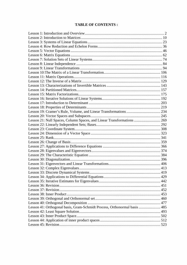
TABLE OF CONTENTS : Lesson 1: Introduction and Overview .................................................................................... 2 Lesson 2: Introduction to Matrices ...................................................................................... 10 Lesson 3: Systems of Linear Equations ............................................................................... 23 Lesson 4: Row Reduction and Echelon Forms .................................................................... 36 Lesson 5: Vector Equations ................................................................................................. 46 Lesson 6: Matrix Equations ................................................................................................. 62 Lesson 7: Solution Sets of Linear Systems .......................................................................... 74 Lesson 8: Linear Independence ........................................................................................... 84 Lesson 9: Linear Transformations ....................................................................................... 94 Lesson 10:The Matrix of a Linear Transformation ............................................................ 106 Lesson 11: Matrix Operations ............................................................................................ 116 Lesson 12: The Inverse of a Matrix ................................................................................... 129 Lesson 13: Characterizations of Invertible Matrices ......................................................... 143 Lesson 14: Partitioned Matrices......................................................................................... 157 Lesson 15: Matrix Factorizations....................................................................................... 175 Lesson 16: Iterative Solutions of Linear Systems .............................................................. 192 Lesson 17: Introduction to Determinant ............................................................................ 203 Lesson 18: Properties of Determinants .............................................................................. 219 Lesson 19: Cramer’s Rule, Volume, and Linear Transformations .................................... 234 Lesson 20: Vector Spaces and Subspaces .......................................................................... 245 Lesson 21: Null Spaces, Column Spaces, and Linear Transformations ............................ 269 Lesson 22: Linearly Independent Sets; Bases .................................................................... 292 Lesson 23: Coordinate System........................................................................................... 308 Lesson 24: Dimension of a Vector Space .......................................................................... 323 Lesson 25: Rank ................................................................................................................. 341 Lesson 26: Change of Basis ............................................................................................... 359 Lesson 27: Applications to Difference Equations ............................................................. 366 Lesson 28: Eigenvalues and Eigenvectors ......................................................................... 374 Lesson 29: The Characteristic Equation ............................................................................ 384 Lesson 30: Diagonalization................................................................................................ 396 Lesson 31: Eigenvectors and Linear Transformations ....................................................... 406 Lesson 32: Complex Eigenvalues ...................................................................................... 413 Lesson 33: Discrete Dynamical Systems ........................................................................... 419 Lesson 34: Applications to Differential Equations ............................................................ 429 Lesson 35: Iterative Estimates for Eigenvalues ................................................................. 442 Lesson 36: Revision ........................................................................................................... 451 Lesson 37: Revision ........................................................................................................... 452 Lesson 38: Inner Product ................................................................................................... 453 Lesson 39: Orthogonal and Orthonormal set ..................................................................... 460 Lesson 40: Orthogonal Decomposition ............................................................................. 477 Lesson 41: Orthogonal basis, Gram-Schmidt Process, Orthonormal basis ....................... 485 Lesson 42: Least Square Solution ...................................................................................... 493 Lesson 43: Inner Product Space ......................................................................................... 502 Lesson 44: Application of inner product spaces ................................................................ 512 Lesson 45: Revision ........................................................................................................... 523

1-Introduction and Overview VU
______________________________________________________________________ ©Virtual University Of Pakistan 2
Lecture 1
Introduction and Overview What is Algebra?
History
Algebra is named in honor of Mohammed Ibn-e- Musa al-Khowârizmî. Around 825, he
wrote a book entitled Hisb al-jabr u'l muqubalah, ("the science of reduction and
cancellation"). His book, Al-jabr, presented rules for solving equations.
Algebra is a branch of Mathematics that uses mathematical statements to describe
relationships between things that vary over time. These variables include things like the
relationship between supply of an object and its price. When we use a mathematical
statement to describe a relationship, we often use letters to represent the quantity that
varies, since it is not a fixed amount. These letters and symbols are referred to as
variables.
Algebra is a part of mathematics in which unknown quantities are found with the help of
relations between the unknown and known.
In algebra, letters are sometimes used in place of numbers.
The mathematical statements that describe relationships are expressed using algebraic
terms, expressions, or equations (mathematical statements containing letters or symbols
to represent numbers). Before we use algebra to find information about these kinds of
relationships, it is important to first introduce some basic terminology.
Algebraic Term
The basic unit of an algebraic expression is a term. In general, a term is either a product of a number and with one or more variables.
For example 4x is an algebraic term in which 4 is coefficient and x is said to be variable.
Study of Algebra
Today, algebra is the study of the properties of operations on numbers. Algebra
generalizes arithmetic by using symbols, usually letters, to represent numbers or
unknown quantities. Algebra is a problem-solving tool. It is like a tractor, which is a

1-Introduction and Overview VU
______________________________________________________________________ ©Virtual University Of Pakistan 3
farmer's tool. Algebra is a mathematician's tool for solving problems. Algebra has
applications to every human endeavor. From art to medicine to zoology, algebra can be a
tool. People who say that they will never use algebra are people who do not know about
algebra. Learning algebra is a bit like learning to read and write. If you truly learn
algebra, you will use it. Knowledge of algebra can give you more power to solve
problems and accomplish what you want in life. Algebra is a mathematicians’ shorthand!
Algebraic Expressions
An expression is a collection of numbers, variables, and +ve sign or –ve sign, of operations that must make mathematical and logical behaviour.
For example 28 9 1x x+ − is an algebraic expression.
What is Linear Algebra? One of the most important problems in mathematics is that of solving systems of linear
equations. It turns out that such problems arise frequently in applications of mathematics
in the physical sciences, social sciences, and engineering. Stated in its simplest terms, the
world is not linear, but the only problems that we know how to solve are the linear ones.
What this often means is that only recasting them as linear systems can solve non-linear
problems. A comprehensive study of linear systems leads to a rich, formal structure to
analytic geometry and solutions to 2x2 and 3x3 systems of linear equations learned in
previous classes.
It is exactly what the name suggests. Simply put, it is the algebra of systems of linear
equations. While you could solve a system of, say, five linear equations involving five
unknowns, it might not take a finite amount of time. With linear algebra we develop
techniques to solve m linear equations and n unknowns, or show when no solution exists.
We can even describe situations where an infinite number of solutions exist, and describe
them geometrically.
Linear algebra is the study of linear sets of equations and their transformation properties.
Linear algebra, sometimes disguised as matrix theory, considers sets and functions, which
preserve linear structure. In practice this includes a very wide portion of mathematics!

1-Introduction and Overview VU
______________________________________________________________________ ©Virtual University Of Pakistan 4
Thus linear algebra includes axiomatic treatments, computational matters, algebraic
structures, and even parts of geometry; moreover, it provides tools used for analyzing
differential equations, statistical processes, and even physical phenomena.
Linear Algebra consists of studying matrix calculus. It formalizes and gives geometrical
interpretation of the resolution of equation systems. It creates a formal link between
matrix calculus and the use of linear and quadratic transformations. It develops the idea
of trying to solve and analyze systems of linear equations.
Applications of Linear algebra
Linear algebra makes it possible to work with large arrays of data. It has many
applications in many diverse fields, such as
• Computer Graphics,
• Electronics,
• Chemistry,
• Biology,
• Differential Equations,
• Economics,
• Business,
• Psychology,
• Engineering,
• Analytic Geometry,
• Chaos Theory,
• Cryptography,
• Fractal Geometry,
• Game Theory,
• Graph Theory,
• Linear Programming,
• Operations Research
It is very important that the theory of linear algebra is first understood, the concepts are
cleared and then computation work is started. Some of you might want to just use the

1-Introduction and Overview VU
______________________________________________________________________ ©Virtual University Of Pakistan 5
computer, and skip the theory and proofs, but if you don’t understand the theory, then it
can be very hard to appreciate and interpret computer results.
Why using Linear Algebra?
Linear Algebra allows for formalizing and solving many typical problems in different
engineering topics. It is generally the case that (input or output) data from an experiment
is given in a discrete form (discrete measurements). Linear Algebra is then useful for
solving problems in such applications in topics such as Physics, Fluid Dynamics, Signal
Processing and, more generally Numerical Analysis.
Linear algebra is not like algebra. It is mathematics of linear spaces and linear functions.
So we have to know the term "linear" a lot. Since the concept of linearity is fundamental
to any type of mathematical analysis, this subject lays the foundation for many branches
of mathematics.
Objects of study in linear algebra
Linear algebra merits study at least because of its ubiquity in mathematics and its
applications. The broadest range of applications is through the concept of vector spaces
and their transformations. These are the central objects of study in linear algebra
1. The solutions of homogeneous systems of linear equations form paradigm
examples of vector spaces. Of course they do not provide the only examples.
2. The vectors of physics, such as force, as the language suggests, also provide
paradigmatic examples.
3. Binary code is another example of a vector space, a point of view that finds
application in computer sciences.
4. Solutions to specific systems of differential equations also form vector spaces.
5. Statistics makes extensive use of linear algebra.
6. Signal processing makes use of linear algebra.
7. Vector spaces also appear in number theory in several places, including the
study of field extensions.
8. Linear algebra is part of and motivates much abstract algebra. Vector spaces
form the basis from which the important algebraic notion of module has been
abstracted.

1-Introduction and Overview VU
______________________________________________________________________ ©Virtual University Of Pakistan 6
9. Vector spaces appear in the study of differential geometry through the tangent
bundle of a manifold.
10. Many mathematical models, especially discrete ones, use matrices to represent
critical relationships and processes. This is especially true in engineering as
well as in economics and other social sciences.
There are two principal aspects of linear algebra: theoretical and computational. A major
part of mastering the subject consists in learning how these two aspects are related and
how to move from one to the other.
Many computations are similar to each other and therefore can be confusing without
reasonable level of grasp of their theoretical context and significance. It will be very
tempting to draw false conclusions.
On the other hand, while many statements are easier to express elegantly and to
understand from a purely theoretical point of view, to apply them to concrete problems
you will need to “get your hands dirty”. Once you have understood the theory sufficiently
and appreciate the methods of computation, you will be well placed to use software
effectively, where possible, to handle large or complex calculations.

1-Introduction and Overview VU
______________________________________________________________________ ©Virtual University Of Pakistan 7
Course Segments
The course is covered in 45 Lectures spanning over six major segments, which are given
below;
1. Linear Equations
2. Matrix Algebra
3. Determinants
4. Vector spaces
5. Eigen values and Eigenvectors, and
6. Orthogonal sets
Course Objectives
The main purpose of the course is to introduce the concept of linear algebra, to explain
the underline theory, the computational techniques and then try to apply them on real life
problems. Mayor course objectives are as under;
• To master techniques for solving systems of linear equations
• To introduce matrix algebra as a generalization of the single-variable algebra of
high school.
• To build on the background in Euclidean space and formalize it with vector space
theory.
• To develop an appreciation for how linear methods are used in a variety of
applications.
• To relate linear methods to other areas of mathematics such as calculus and,
differential equations.

1-Introduction and Overview VU
______________________________________________________________________ ©Virtual University Of Pakistan 8
Recommended Books and Supported Material I am indebted to several authors whose books I have freely used to prepare the lectures
that follow. The lectures are based on the material taken from the books mentioned
below.
1. Linear Algebra and its Applications (3rd Edition) by David C. Lay.
2. Contemporary Linear Algebra by Howard Anton and Robert C. Busby.
3. Introductory Linear Algebra (8th Edition) by Howard Anton and Chris Rorres.
4. Introduction to Linear Algebra (3rd Edition) by L. W. Johnson, R.D. Riess and
J.T. Arnold.
5. Linear Algebra (3rd Edition) by S. H. Friedberg, A.J. Insel and L.E. Spence.
6. Introductory Linear Algebra with Applications (6th Edition) by B. Kolman.
I have taken the structure of the course as proposed in the book of David C. Lay. I would
be following this book. I suggest that the students should purchase this book, which is
easily available in the market and also does not cost much. For further study and
supplement, students can consult any of the above mentioned books.
I strongly suggest that the students should also browse on the Internet; there is plenty of
supporting material available. In particular, I would suggest the website of David C. Lay;
www.laylinalgebra.com, where the entire material, study guide, transparencies are readily
available. Another very useful website is www.wiley.com/college/anton, which contains a
variety of useful material including the data sets. A number of other books are also
available in the market and on the internet with free access.
I will try to keep the treatment simple and straight. The lectures will be presented in
simple Urdu and easy English. These lectures are supported by the handouts in the form
of lecture notes. The theory will be explained with the help of examples. There will be
enough exercises to practice with. Students are advised to go through the course on daily
basis and do the exercises regularly.
1-Introduction and Overview VU
______________________________________________________________________ ©Virtual University Of Pakistan 9
Schedule and Assessment
The course will be spread over 45 lectures. Lectures one and two will be introductory and
the Lecture 45 will be the summary. The first two lectures will lay the foundations and
would provide the overview of the course. These are important from the conceptual point
of view. I suggest that these two lectures should be viewed again and again.
The course will be interesting and enjoyable, if the student will follow it regularly and
completes the exercises as they come along. To follow the tradition of a semester system
or of a term system, there will be a series of assignments (Max eight assignments) and a
mid term exam. Finally there will be terminal examination.
The assignments have weights and therefore they have to be taken seriously.

2-Introduction to Matrices VU
©Virtual University Of Pakistan 10
Lecture 2 Background
Introduction to Matrices Matrix A matrix is a collection of numbers or functions arranged into rows and columns. Matrices are denoted by capital letters ZYBA ,,,, . The numbers or functions are called elements of the matrix. The elements of a matrix are denoted by small letters zyba ,,,, . Rows and Columns The horizontal and vertical lines in a matrix are, respectively, called the rows and columns of the matrix. Order of a Matrix The size (or dimension) of matrix is called as order of matrix. Order of matrix is based on the number of rows and number of columns. It can be written as r c× ; r means no. of row and c means no. of columns. If a matrix has m rows and n columns then we say that the size or order of the matrix is nm× . If A is a matrix having m rows and n columns then the matrix can be written as
11 12 1
21 22 2
1 2
n
n
m m mn
a a aa a a
A
a a a
=
The element, or entry, in the ith row and jth column of a nm× matrix A is written as ija
For example: The matrix 2 1 30 4 6
A−
=
has two rows and three columns. So order of A
will be 2 3× Square Matrix A matrix with equal number of rows and columns is called square matrix.
For Example The matrix 4 7 89 3 51 1 2
A−
= −
has three rows and three columns. So it is a
square matrix of order 3.
Equality of matrices
The two matrices will be equal if they must have

2-Introduction to Matrices VU
©Virtual University Of Pakistan 11
a) The same dimensions (i.e. same number of rows and columns) b) Corresponding elements must be equal.
Example The matrices 4 7 89 3 51 1 2
A−
= −
and 4 7 89 3 51 1 2
B−
= −
equal matrices
(i.e A = B) because they both have same orders and same corresponding elements. Column Matrix A column matrix X is any matrix having n rows and only one column. Thus the column matrix X can be written as
11
1
31
21
11
][ ×=
= ni
n
b
b
b
b
b
X
A column matrix is also called a column vector or simply a vector. Multiple of matrix A multiple of a matrix A by a nonzero constant k is defined to be
nmij
mnmm
n
n
ka
kakaka
kakaka
kakaka
kA ×=
= ][
21
22221
11211
Notice that the product kA is same as the product Ak . Therefore, we can write AkkA = . It implies that if we multiply a matrix by a constant k, then each element of the matrix is to be multiplied by k. Example 1
(a)
−
−
=
−
−
⋅
301
520
1510
65/1
14
32
5

2-Introduction to Matrices VU
©Virtual University Of Pakistan 12
(b)
−=
−⋅
t
t
t
t
e
e
e
e
4
2
4
2
1
Since we know that AkkA = . Therefore, we can write
tt
tt e
e
ee 3
3
33
5
2
5
2
5
2−
−
−−
=
=
⋅
Addition of Matrices Only matrices of the same order may be added by adding corresponding elements. If ][ ijaA = and ][ ijbB = are two nm× matrices then ][ ijij baBA +=+ Obviously order of the matrix A + B is nm× Example 2 Consider the following two matrices of order 33×
−−
−
=
5106
640
312
A ,
−
−
=
211
539
874
B
Since the given matrices have same orders, therefore, these matrices can be added and their sum is given by
−−
−
=
+−−++−
+++
−++−+
=+
395
1179
566
25)1(1016
563490
)8(37142
BA
Example 3 Write the following single column matrix as the sum of three column vectors
+−
tttet t
5723
2
2
Solution

2-Introduction to Matrices VU
©Virtual University Of Pakistan 13
2 2
2 2 2
3 2 3 0 2 3 0 27 7 0 1 7 0
5 0 5 0 0 5 0
t t
t
t e t et t t t t t e
t t
− − − + = + + = + +
Difference of Matrices The difference of two matrices A and B of same order nm× is defined to be the matrix )( BABA −+=− The matrix B− is obtained by multiplying the matrix B with 1− . So that BB ) 1 ( −=− Multiplication of Matrices We can multiply two matrices if and only if, the number of columns in the first matrix equals the number of rows in the second matrix. Otherwise, the product of two matrices is not possible. OR If the order of the matrix A is nm× then to make the product AB possible order of the matrix B must be pn× . Then the order of the product matrix AB is pm× . Thus pmpnnm CBA ××× =⋅ If the matrices A and B are given by
=
=
npnn
p
p
mnmm
n
n
bbb
bbb
bbb
B
aaa
aaa
aaa
A
21
22221
11211
21
22221
11211
,
Then
=
npnn
p
p
mnmm
n
n
bbb
bbb
bbb
aaa
aaa
aaa
AB
21
22221
11211
21
22221
11211
=
11 11 12 21 1 1 11 1 12 2 1
21 11 22 21 2 1 21 1 22 2 2
1 11 2 21 1 1 1 2 2
n n p p n np
n n p p n np
m m mn n m p m p mn np
a b a b a b a b a b a ba b a b a b a b a b a b
a b a b a b a b a b a b
+ + + + + + + + + + + + + + + + + +

2-Introduction to Matrices VU
©Virtual University Of Pakistan 14
pn
n
kkjikba
×=
= ∑
1
Example 4 If possible, find the products AB and BA , when
(a)
=
53
74A ,
−=
86
29B
(b)
=
7
0
8
2
1
5
A ,
−−=
02
34B
Solution (a) The matrices A and B are square matrices of order 2. Therefore, both of the products AB and BA are possible.
=
⋅+−⋅⋅+⋅
⋅+−⋅⋅+⋅=
−
=
3457
4878
85)2(36593
87)2(46794
86
29
53
74AB
Similarly
=
⋅+⋅⋅+⋅
⋅−+⋅⋅−+⋅=
−=
8248
5330
58763846
5)2(793)2(49
53
74
86
29BA
Note From above example it is clear that generally a matrix multiplication is not commutative i.e. BAAB ≠ . (b) The product AB is possible as the number of columns in the matrix A and the number of rows in B is 2. However, the product BA is not possible because the number of column in the matrix B and the number of rows in A is not same.
5 84 3
1 02 0
2 7
5 ( 4) 8 2 5 ( 3) 8 0 4 151 ( 4) 0 2 1 ( 3) 0 0 4 32 ( 4) 7 2 2 ( 3) 7 0 6 6
AB
− − =
⋅ − + ⋅ ⋅ − + ⋅ − − = ⋅ − + ⋅ ⋅ − + ⋅ = − − ⋅ − + ⋅ ⋅ − + ⋅ −
=
3457
4878AB ,
=
8248
5330BA
Clearly .BAAB ≠

2-Introduction to Matrices VU
©Virtual University Of Pakistan 15
−
−
−
−
−
=
6
3
15
6
4
4
AB
However, the product BA is not possible. Example 5
(a)
−
=
⋅+⋅−+−⋅
⋅+⋅+−⋅
⋅+⋅−+−⋅
=
−
−
−
9
44
0
496)7()3(1
6564)3(0
436)1()3(2
4
6
3
971
540
312
(b)
+
+−=
−
yx
yx
y
x
83
24
83
24
Multiplicative Identity For a given any integer n , the nn× matrix
=
1000
0100
0010
0001
I
is called the multiplicative identity matrix. If A is a matrix of order n n× , then it can be verified that AIAAI =⋅=⋅
Example 1 00 1
I =
, 1 0 00 1 00 0 1
I =
are identity matrices of orders 2 x 2 and 3 x 3
respectively and If
−=
86
29B then we can easily prove that BI = IB = B

2-Introduction to Matrices VU
©Virtual University Of Pakistan 16
Zero Matrix or Null matrix A matrix whose all entries are zero is called zero matrix or null matrix and it is denoted byO .
For example
=
0
0O ;
=
00
00O ;
=
0
0
0
0
0
0
O
and so on. If A and O are the matrices of same orders, then AAOOA =+=+ Associative Law The matrix multiplication is associative. This means that if BA , and C are pm× , rp× and nr × matrices, then CABBCA )()( = The result is a nm× matrix. This result can be verified by taking any three matrices which are confirmable for multiplication. Distributive Law If B and C are matrices of order nr × and A is a matrix of order rm× , then the distributive law states that ACABCBA +=+ )( Furthermore, if the product CBA )( + is defined, then BCACCBA +=+ )( Remarks It is important to note that some rules arithmetic for real numbers do not carry over the matrix arithmetic. For example, , , anda b c d∀ ∈
i) if ab cd= and 0a ≠ , then b c= (Law of Cancellation) ii) if 0ab = , then least one of the factors a or b (or both) are zero.
However the following examples shows that the corresponding results are not true in case of matrices. Example
Let 0 1 1 1 2 5
, ,0 2 3 4 3 4
A B C = = =
and 1 70 0
D =
, then one can easily check that
3 46 8
AB AC = =
. But B C≠ .
Similarly neither A nor B are zero matrices but 0 00 0
AD =
But if D is diagonal say1 00 7
D =
, then AD DA≠ .
Determinant of a Matrix Associated with every square matrix A of constants, there is a number called the determinant of the matrix, which is denoted by )det(A or A . There is a special way to find the determinant of a given matrix.

2-Introduction to Matrices VU
©Virtual University Of Pakistan 17
Example 6 Find the determinant of the following matrix
−
=
421
152
263
A
Solution The determinant of the matrix A is given by
421
152
263
)det(
−
=A
We expand the )det(A by first row, we obtain
421
152
263
)det(
−
=A =34215
-64112
−+2
2152
−
or 185)2(41)6(8-2)-3(20)det( =+++=A Transpose of a Matrix The transpose of nm× matrix A is denoted by trA and it is obtained by interchanging rows of A into its columns. In other words, rows of A become the columns of .trA Clearly trA is n m× matrix.
If
11 12 1
21 22 2
1 2
n
n
m m mn
a a aa a a
A
a a a
=
, then
11 21 1
12 22 2
1 2
m
mtr
n n mn
a a aa a a
A
a a a
=
Since order of the matrix A is nm× , the order of the transpose matrix trA is mn× .
Properties of the Transpose
The following properties are valid for the transpose;
• The transpose of the transpose of a matrix is the matrix itself:` • The transpose of a matrix times a scalar (k) is equal to the constant times the
transpose of the matrix: ( )T T T TABC C B A= ( )T TkA kA= • The transpose of the sum of two matrices is equivalent to the sum of their
transposes: ( )T T TA B A B+ = + • The transpose of the product of two matrices is equivalent to the product of their
transposes in reversed order: ( )T T TAB B A= • The same is true for the product of multiple matrices: ( )T T T TABC C B A=

2-Introduction to Matrices VU
©Virtual University Of Pakistan 18
Example 7 (a) The transpose of matrix
−
=
421
152
263
A is 3 2 1
6 5 22 1 4
TA−
=
(b) If
=
3
0
5
X , then [ ]5 0 3TX =
Multiplicative Inverse Suppose that A is a square matrix of order nn× . If there exists an
nn× matrix B such that IBAAB == , then B is said to be the multiplicative inverse of the matrix A and is denoted by 1−= AB .
For example: If
=
102
41A then the matrix B
5 21 1/ 2
− = −
is multiplicative inverse of A
because AB = 1 42 10
5 21 1/ 2
− −
= 1 00 1
=I
Similarly we can check that BA = I Singular and Non-Singular Matrices A square matrix A is said to be a non-singular matrix ifdet( ) 0A ≠ , otherwise the square matrix A is said to be singular. Thus for a singular matrix A we must have det( ) 0A =
Example: 2 3 11 1 02 3 5
A−
= −
2(5 0) 3(5 0) 1( 3 2)
10 15 5 0A = − − − − − −
= − + =
which means that A is singular. Minor of an element of a matrix Let A be a square matrix of order n x n. Then minor ijM of the element ija A∈ is the determinant of )1()1( −×− nn matrix obtained by deleting the ith row and jth column from A .
2-Introduction to Matrices VU
©Virtual University Of Pakistan 19
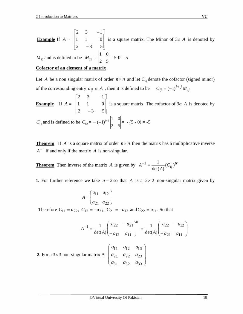
Example If 2 3 11 1 02 3 5
A−
= −
is a square matrix. The Minor of 3 A∈ is denoted by
12M and is defined to be 12M = 1 02 5
= 5-0 = 5
Cofactor of an element of a matrix Let A be a non singular matrix of order nn× and let C ij denote the cofactor (signed minor)
of the corresponding entry ija A∈ , then it is defined to be ijji
ij MC +−= )1(
Example If 2 3 11 1 02 3 5
A−
= −
is a square matrix. The cofactor of 3 A∈ is denoted by
12C and is defined to be 12C = 1 2 1 0( 1)
2 5+= − = - (5 - 0) = -5
Theorem If A is a square matrix of order nn× then the matrix has a multiplicative inverse
1−A if and only if the matrix A is non-singular.
Theorem Then inverse of the matrix A is given by trijC
AA )(
)det(11 =−
1. For further reference we take 2=n so that A is a 22× non-singular matrix given by
=
2221
1211
aa
aaA
Therefore 122121122211 , , aCaCaC −=−== and 1122 aC = . So that
−
−=
−
−=−
1121
1222
1112
21221)det(
1)det(
1aa
aa
Aaa
aa
AA
tr
2. For a 3×3 non-singular matrix A=11 12 13
21 22 23
31 32 33
a a aa a aa a a

2-Introduction to Matrices VU
©Virtual University Of Pakistan 20
3332
232211
aa
aaC = ,
3331
232112
aa
aaC −= , C13 =
3231
2221
aaaa
and so on.
Therefore, inverse of the matrix A is given by 11 21 31
112 22 32
13 23 33
1det
C C CA C C C
AC C C
−
=
.
Example 8 Find, if possible, the multiplicative inverse for the matrix
=
102
41A .
Solution The matrix A is non-singular because 2=8-10=102
41)det( =A
Therefore, 1−A exists and is given by A 1− =
−
−=
−
−
2/11
25
12
410
21
Check IAA =
=
+−−
+−−=
−
−
=−
10
01
541010
2245
2/11
25
102
411
IAA =
=
+−+−
−−=
−
−=−
10
01
5411
202045
102
41
2/11
251
Example 9 Find, if possible, the multiplicative inverse of the following matrix
=
33
22A
Solution The matrix is singular because
0323233
22)det( =⋅−⋅==A
Therefore, the multiplicative inverse 1−A of the matrix does not exist.
Example 10 Find the multiplicative inverse for the following matrix
A=2 2 02 1 1
3 0 1−
.

2-Introduction to Matrices VU
©Virtual University Of Pakistan 21
Solution Since 012)30(0)32(2)01(2
103
112
022
)det( ≠=−+−−−−=−=A
Therefore, the given matrix is non singular. So, the multiplicative inverse 1−A of the matrix A exists. The cofactors corresponding to the entries in each row are
303
12 ,5
13
12 ,1
10
11131211 −=
−==
−−=== CCC
603
22 ,2
13
02 ,2
10
02232221 =−===−=−= CCC
612
22 ,2
12
02 ,2
11
02333231 =
−=−=
−−=== CCC
Hence A 1− =121
−−
−
663225
221=
−−
−
2/12/14/16/16/112/5
6/16/112/1
We can also verify that IAAAA =⋅=⋅ −− 11 Derivative of a Matrix of functions Suppose that
( ) ( )ij m nA t a t
× =
is a matrix whose entries are functions those are differentiable in a common interval, then derivative of the matrix )(tA is a matrix whose entries are derivatives of the corresponding entries of the matrix )(tA . Thus
nm
ijdt
dadtdA
×
=
The derivative of a matrix is also denoted by ).(tA′ Integral of a Matrix of Functions Suppose that ( ) nmij tatA
×= )()( is a matrix whose entries are functions those are continuous
on a common interval containing t , then integral of the matrix )(tA is a matrix whose entries are integrals of the corresponding entries of the matrix )(tA . Thus
0
0
( ) ( )ijm n
t tA s ds a s dstt ×
= ∫ ∫

2-Introduction to Matrices VU
©Virtual University Of Pakistan 22
Example 11 Find the derivative and the integral of the following matrix
sin 23( )
8 1
ttX t e
t=
−
Solution The derivative and integral of the given matrix are, respectively, given by
=
−
=′
8
3
2cos2
)18(
)(
)2(sin
)( 33 tt e
t
tdtd
edtd
tdtd
tX and
0
3 3
20
0
sin 2
1/ 2cos 2 1/ 2( ) 1/ 3 1/ 3
0 4
8 1
t
ts t
t
sds
ttX s ds e ds e
t t
s ds
− + = = − − −
∫
∫ ∫
∫
Exercise Write the given sum as a single column matrix
1. ( )
−−
−−
−+
− t
ttttt
543
23
11
1
23
2. 1 3 4 22 5 1 2 1 1 80 4 2 4 6
t tt
t
− − − − + − − − − −
Determine whether the given matrix is singular or non-singular. If singular, find 1A− .
3. 3 2 14 1 02 5 1
A = − −
4. 4 1 16 2 32 1 2
A−
= − − −
Find dXdt
5.
+−
−=
tt
ttX
2cos52sin3
2cos42sin21
6. If ( )4
2
cos
2 3 1
te tA t
t t
π = −
then find (a) ∫2
0
)( dttA , (b) ∫t
dssA0
.)(
7. Find the integral ∫2
1
)( dttB if ( )6 2
1/ 4t
B tt t
=

3-System of Linear Equations VU
©Virtual University Of Pakistan 23
Lecture 3
Systems of Linear Equations In this lecture we will discuss some ways in which systems of linear equations arise, how to solve them, and how their solutions can be interpreted geometrically. Linear Equations We know that the equation of a straight line is written as y mx c= + , where m is the slope of line(Tan of the angle of line with x-axis) and c is the y-intercept(the distance at which the straight line meets y-axis from origin). Thus a line in R2 (2-dimensions) can be represented by an equation of the form
1 2a x a y b+ = (where a1, a2 not both zero). Similarly a plane in R3 (3-dimensional space) can be represented by an equation of the form 1 2 3a x a y a z b+ + = (where a1, a2, a3 not all zero). A linear equation in n variables 1 2, , , nx x x can be expressed in the form
1 1 2 2 n na x a x a x b+ + + = (hyper plane in n ) --------(1)
where 1 2, , , na a a and b are constants and the “a’s” are not all zero. Homogeneous Linear equation In the special case if b = 0, Equation (1) has the form 1 1 2 2 0n na x a x a x+ + + = (2) This equation is called homogeneous linear equation. Note A linear equation does not involve any products or square roots of variables. All variables occur only to the first power and do not appear, as arguments of trigonometric, logarithmic, or exponential functions. Examples of Linear Equations (1) The equations
( )1 2 3 2 1 32 3 2 2 5 2x x x and x x x+ + = = + + are both linear
(2) The following equations are also linear 1 2 3 4
11 22
3 7 2 3 0
3 1 1n
x y x x x x
x y z x x x
+ = − − + =
− + = − + + + =
(3) The equations 1 2 1 2 2 13 2 4 6x x x x and x x− = = −
are not linear because of the presence of 1 2x x in the first equation and 1x in the second.
3-System of Linear Equations VU
©Virtual University Of Pakistan 24
System of Linear Equations A finite set of linear equations is called a system of linear equations or linear system. The variables in a linear system are called the unknowns. For example,
1 2 3
1 2 3
4 3 13 9 4
x x xx x x− + = −+ + = −
is a linear system of two equations in three unknowns x1, x2, and x3. General System of Linear Equations A general linear system of m equations in n-unknowns 1 2, , , nx x x can be written as
11 1 12 2 1 1
21 1 22 2 2 2
1 1 2 2
n n
n n
m m mn n m
a x a x a x ba x a x a x b
a x a x a x b
+ + + =+ + + =
+ + + =
(3)
Solution of a System of Linear Equations A solution of a linear system in the unknowns 1 2, , , nx x x is a sequence of n numbers
1 2, , , ns s s such that when substituted for 1 2, , , nx x x respectively, makes every equation in the system a true statement. The set of all such solutions { }1 2, , , ns s s of a linear system is called its solution set. Linear System with Two Unknowns When two lines intersect in R2, we get system of linear equations with two unknowns
For example, consider the linear system 1 1 1
2 2 2
a x b y ca x b y c
+ =+ =
The graphs of these equations are straight lines in the xy-plane, so a solution (x, y) of this system is infact a point of intersection of these lines. Note that there are three possibilities for a pair of straight lines in xy-plane:
1. The lines may be parallel and distinct, in which case there is no intersection and
consequently no solution. 2. The lines may intersect at only one point, in which case the system has exactly
one solution. 3. The lines may coincide, in which case there are infinitely many points of
intersection (the points on the common line) and consequently infinitely many solutions.

3-System of Linear Equations VU
©Virtual University Of Pakistan 25
Consistent and inconsistent system A linear system is said to be consistent if it has at least one solution and it is called inconsistent if it has no solutions. Thus, a consistent linear system of two equations in two unknowns has either one solution or infinitely many solutions – there is no other possibility. Example consider the system of linear equations in two variables
1 2 1 22 1, 3 3x x x x− = − − + = Solve the equation simultaneously: Adding both equations we get 2x = 2, Put 2x = 2 in any one of the above equation we get 1 3x = . So the solution is the single point (3, 2). See the graph of this linear system
x2 2 x1 l2 3 l1 (a) This system has exactly one solution See the graphs to the following linear systems:
1 2
1 2
( ) 2 12 3
a x xx x− = −
− + = 1 2
1 2
( ) 2 12 1
b x xx x− = −
− + =
x2 x2 2 2 x1 l2 3 3 l1 l1 (a) (b)
(a) No solution. (b) Infinitely many solutions.

3-System of Linear Equations VU
©Virtual University Of Pakistan 26
Linear System with Three Unknowns Consider r a linear system of three equations in three unknowns:
1 1 1 1
2 2 1 2
3 3 3 3
a x b y c z da x b y c z da x b y c z d
+ + =+ + =+ + =
In this case, the graph of each equation is a plane, so the solutions of the system, If any correspond to points where all three planes intersect; and again we see that there are only three possibilities – no solutions, one solution, or infinitely many solutions as shown in figure.
Theorem 1 Every system of linear equations has zero, one or infinitely many solutions; there are no other possibilities.
Example 1 Solve the linear system 1
2 6x yx y− =+ =
Solution
Adding both equations, we get 73
x = . Putting this value of x in 1st equation, we
get 43
y = . Thus, the system has the unique solution 7 4, .3 3
x y= =
Geometrically, this means that the lines represented by the equations in the system
intersect at a single point 7 4,3 3
and thus has a unique solution.
Example 2 Solve the linear system 4
3 3 6x yx y+ =+ =
Solution Multiply first equation by 3 and then subtract the second equation from this. We obtain 0 6= This equation is contradictory.

3-System of Linear Equations VU
©Virtual University Of Pakistan 27
Geometrically, this means that the lines corresponding to the equations in the original system are parallel and distinct. So the given system has no solution.
Example 3 Solve the linear system 4 2 1
16 8 4x yx y− =− =
Solution Multiply the first equation by -4 and then add in second equation.
16 8 416 8 4
0 0
x yx y
− + = −− =
=
Thus, the solutions of the system are those values of x and y that satisfy the single equation 4 2 1x y− = Geometrically, this means the lines corresponding to the two equations in the original system coincide and thus the system has infinitely many solutions. Parametric Representation It is very convenient to describe the solution set in this case is to express it parametrically. We can do this by letting y = t and solving for x in terms of t, or by letting x = t and solving for y in terms of t. The first approach yields the following parametric equations (by taking y=t in the equation 4 2 1x y− = )
4 2 1,1 1 ,4 2
x t y t
x t y t
− = =
= + =
We can now obtain some solutions of the above system by substituting some numerical values for the parameter.
Example For t = 0 the solution is 1( ,0).4
For t = 1, the solution is 3( ,1)4
and for 1t = −
the solution is 1( , 1) .4
etc− −
Example 4 Solve the linear system 2 5
2 2 4 103 3 6 15
x y zx y zx y z
− + =− + =− + =

3-System of Linear Equations VU
©Virtual University Of Pakistan 28
Solution Since the second and third equations are multiples of the first. Geometrically, this means that the three planes coincide and those values of x, y and z that satisfy the equation 2 5x y z− + = automatically satisfy all three equations. We can express the solution set parametrically as 1 2 1 25 2 , ,x t t y t z t= + − = = Some solutions can be obtained by choosing some numerical values for the parameters. For example if we take 1 2y t= = and 2 3z t= = then
1 25 25 2 2(3)1
x t t= + −= + −=
Put these values of x, y, and z in any equation of linear system to verify
2 51 2 2(3) 51 2 6 55 5
x y z− + =− + =− + ==
Hence x = 1, y = 2, z = 3 is the solution of the system. Verified. Matrix Notation The essential information of a linear system can be recorded compactly in a rectangular array called a matrix.
Given the system 1 2 3
2 3
1 2 3
2 02 8 8
4 5 9 9
x x xx x
x x x
− + =− =
− + + = −
With the coefficients of each variable aligned in columns, the matrix 1 2 10 2 84 5 9
− − −
is called the coefficient matrix (or matrix of coefficients) of the system. An augmented matrix of a system consists of the coefficient matrix with an added column containing the constants from the right sides of the equations. It is always denoted by Ab

3-System of Linear Equations VU
©Virtual University Of Pakistan 29
Ab = 1 2 1 00 2 8 84 5 9 9
− − − −
Solving a Linear System In order to solve a linear system, we use a number of methods. 1st of them is given below. Successive elimination method In this method the 1x term in the first equation of a system is used to eliminate the 1x terms in the other equations. Then we use the 2x term in the second equation to eliminate the 2x terms in the other equations, and so on, until we finally obtain a very simple equivalent system of equations.
Example 5 Solve 1 2 3
2 3
1 2 3
2 02 8 8
4 5 9 9
x x xx x
x x x
− + =− =
− + + = −
Solution We perform the elimination procedure with and without matrix notation, and place the results side by side for comparison:
1 2 3
2 3
1 2 3
2 02 8 8
4 5 9 9
x x xx x
x x x
− + =− =
− + + = −
1 2 1 00 2 8 84 5 9 9
− − − −
To eliminate the 1x term from third equation add 4 times equation 1 to equation 3,
1 2 34 8 4 0x x x− + =
1 2 34 5 9 9x x x− + + = −
2 33 13 9x x− + = − The result of the calculation is written in place of the original third equation:
1 2 3
2 3
2 3
2 0
2 8 8
3 13 9
x x xx xx x
− + =
− =
− + = −
1 2 1 00 2 8 80 3 13 9
− − − −
Next, multiply equation 2 by ½ in order to obtain 1 as the coefficient for 2x

3-System of Linear Equations VU
©Virtual University Of Pakistan 30
1 2 3
2 3
2 3
2 0
4 4
3 13 9
x x xx xx x
− + =
− =
− + = −
1 2 1 00 1 4 40 3 13 9
− − − −
To eliminate the 2x term from third equation add 3 times equation 2 to equation 3,
The new system has a triangular form
1 2 3
2 3
3
2 04 43
x x xx xx
− + =− ==
1 2 1 00 1 4 40 0 1 3
− −
Now using 3rd equation eliminate the x3 term from first and second equation i.e. multiply 3rd equation with 4 and add in second equation. Then subtract the third equation from first equation we get
1 2
2
3
2 3163
x xxx
− = −==
1 2 0 30 1 0 160 0 1 3
− −
Adding 2 times equation 2 to equation 1, we obtain the result
1
2
3
29 1 0 0 2916 0 1 0 16
0 0 1 33
xxx
= = =
This completes the solution. Our work indicates that the only solution of the original system is (29, 16, 3). To verify that (29, 16, 3) is a solution, substitute these values into the left side of the original system for x1, x2 and x3 and after computing, we get (29) – 2(16) + (3) = 29 – 32 + 3 = 0 2(16) – 8(3) = 32 – 24 = 8 –4(29) + 5(16) + 9(3) = –116 + 80 + 27 = –9 The results agree with the right side of the original system, so (29, 16, 3) is a solution of the system.

3-System of Linear Equations VU
©Virtual University Of Pakistan 31
This example illustrates how operations on equations in a linear system correspond to operations on the appropriate rows of the augmented matrix. The three basic operations listed earlier correspond to the following operations on the augmented matrix. Elementary Row Operations 1. (Replacement) Replace one row by the sum of itself and a nonzero multiple of
another row. 2. (Interchange) Interchange two rows. 3. (Scaling) Multiply all entries in a row by a nonzero constant. Row equivalent matrices A matrix B is said to be row equivalent to a matrix A of the same order if B can be obtained from A by performing a finite sequence of elementary row operations of A. If A and B are row equivalent matrices, then we write this expression mathematically as A B.
For example 1 2 1 00 2 8 84 5 9 9
− − − −
1 2 1 00 2 8 80 3 13 9
− − − −
are row equivalent matrices
because we add 4 times of 1st row in 3rd row in 1st matrix. Note If the augmented matrices of two linear systems are row equivalent, then the two systems have the same solution set. Row operations are extremely easy to perform, but they have to be learnt and practice. Two Fundamental Questions
1. Is the system consistent; that is, does at least one solution exist? 2. If a solution exists is it the only one; that is, is the solution unique?
We try to answer these questions via row operations on the augmented matrix. Example 6 Determine if the following system of linear equations is consistent
1 2 3
2 3
1 2 3
2 02 8 8
4 5 9 9
x x xx x
x x x
− + =− =
− + + = −
Solution First obtain the triangular matrix by removing x1 and x2 term from third equation and removing x2 from second equation.

3-System of Linear Equations VU
©Virtual University Of Pakistan 32
First divide the second equation by 2 we get
1 2 3
2 3
1 2 3
2 04 4
4 5 9 9
x x xx x
x x x
− + =− =
− + + = −
1 2 1 00 1 4 44 5 9 9
− − − −
Now multiply equation 1 with 4 and add in equation 3 to eliminate x1
from third equation.
1 2 3
2 3
2 3
2 04 4
3 13 9
x x xx xx x
− + =− =
− + = −
1 2 1 00 1 4 40 3 13 9
− − − −
Now multiply equation 2 with 3 and add in equation 3 to eliminate x2
from third equation.
1 2 3
2 3
3
2 04 43
x x xx xx
− + =− ==
1 2 1 00 1 4 40 0 1 3
− −
Put value of x3 in second equation we get
2 4(3) 4x − =
2 16x =
Now put these values of x2 and x3 in first equation we get
1 2(16) 3 0x − + =
1 29x = So a solution exists and the system is consistent and has a unique solution. Example 7 Solve if the following system of linear equations is consistent.
2 3
1 2 3
1 2 3
4 82 3 2 15 8 7 1
x xx x xx x x
− =− + =− + =

3-System of Linear Equations VU
©Virtual University Of Pakistan 33
Solution The augmented matrix is 0 1 4 82 3 2 15 8 7 1
− − −
To obtain x1 in the first equation, interchange rows 1 and 2:
2 3 2 10 1 4 85 8 7 1
− − −
To eliminate the 5x1 term in the third equation, add –5/2 times row 1 to row 3:
2 3 2 10 1 4 80 1/ 2 2 3/ 2
− − − −
Next, use the x2 term in the second equation to eliminate the –(1/2) x2 term from the third equation. Add ½ times row 2 to row 3:
2 3 2 10 1 4 80 0 0 5 / 2
− −
The augmented matrix is in triangular form. To interpret it correctly, go back to equation notation:
1 2 3
2 3
2 3 2 1
4 8
0 2.5
x x xx x
− + =
− =
=
There are no values of x1, x2, x3 that will satisfy because the equation 0 = 2.5 is never true. Hence original system is inconsistent (i.e., has no solution).

3-System of Linear Equations VU
©Virtual University Of Pakistan 34
Exercises 1. State in words the next elementary “row” operation that should be performed on the
system in order to solve it. (More than one answer is possible in (a).)
1 2 3 4
2 3 4
3 4
3 4
. 4 2 8 127 2 45 7
3 5
a x x x xx x x
x xx x
+ − + =− + = −
− =+ = −
1 2 3 4
2 3
3
4
. 3 5 2 08 42 7
1
b x x x xx x
xx
− + − =
+ = −==
2. The augmented matrix of a linear system has been transformed by row operations into
the form below. Determine if the system is consistent.
1 5 2 60 4 7 20 0 5 0
− −
3. Is (3, 4, –2) a solution of the following system?
1 2 3
1 2 3
1 2 3
5 2 72 6 9 07 5 3 7
x x xx x xx x x
− + =− + + =− + − = −
4. For what values of h and k is the following system consistent?
1 2
1 2
26 3
x x hx x k− =
− + =
Solve the systems in the exercises given below;
5. 2 3
1 2 3
1 2 3
5 4
4 3 2
2 7 1
x xx x xx x x
+ = −
+ + = −
+ + = −
6. 1 2 3
1 2 3
1 2 3
5 4 32 7 3 2
2 7 1
x x xx x xx x x
− + = −− + = −
− − =
7. 1 2
1 2 3
2 3
2 4
3 3 2
0
x xx x x
x x
+ =
− − =
+ =
8. 1 3
2 3
1 2 3
2 4 103 2
3 5 8 6
x xx x
x x x
− = −+ =
+ + = −
3-System of Linear Equations VU
©Virtual University Of Pakistan 35
Determine the value(s) of h such that the matrix is augmented matrix of a consistent linear system.
9. 1 32 6 5
h− − −
10. 1 24 2 10
h − −
Find an equation involving g, h, and that makes the augmented matrix correspond to a consistent system.
11. 1 4 70 3 52 5 9
ghk
− − − −
12. 2 5 34 7 46 3 1
ghk
− − − −
Find the elementary row operations that transform the first matrix into the second, and then find the reverse row operation that transforms the second matrix into first.
13. 1 3 1 1 3 10 2 4 , 0 1 20 3 4 0 3 4
− − − − − −
14. 0 5 3 1 5 21 5 2 , 0 5 32 1 8 2 1 8
− − − −
15. 1 3 1 5 1 3 1 50 1 4 2 , 0 1 4 20 2 5 1 0 0 3 5
− − − − − − −

4-Row Reduction and Echelon Forms VU
©Virtual University Of Pakistan 36
Lecture 4
Row Reduction and Echelon Forms To analyze system of linear equations, we shall discuss how to refine the row reduction algorithm. While applying the algorithm to any matrix, we begin by introducing a non zero row or column (i.e. contains at least one nonzero entry) in a matrix, Echelon form of a matrix A rectangular matrix is in echelon form (or row echelon form) if it has the following three properties:
1. All nonzero rows are above any rows of all zeros 2. Each leading entry of a row is in a column to the right of the leading entry of the
row above it. 3. All entries in a column below a leading entry are zero.
Reduced Echelon Form of a matrix If a matrix in echelon form satisfies the following additional conditions, then it is in reduced echelon form (or reduced row echelon form):
4. The leading entry in each nonzero row is 1. 5. Each leading 1 is the only nonzero entry in its column.
Examples of Echelon Matrix form The following matrices are in echelon form. The leading entries ( ) may have any nonzero value; the started entries (*) may have any values (including zero).
2 3 2 11. 0 1 4 8
0 0 0 5 / 2
− −

4-Row Reduction and Echelon Forms VU
©Virtual University Of Pakistan 37
0 * * * * * * * ** * *
0 0 0 * * * * * *0 * *
2. 3. 0 0 0 0 * * * * *0 0 0 0
0 0 0 0 0 * * * *0 0 0 0
0 0 0 0 0 0 0 0 *
1 4 3 7 1 1 04. 0 1 6 2 5. 0 1 0
0 0 1 5 0 0 0
0 1 2 6 06. 0 0 1 1 0
0 0 0 0 1
−
−
Examples of Reduced Echelon Form The following matrices are in reduced echelon form because the leading entries are 1’s, and there are 0’s below and above each leading 1.
1 0 0 291. 0 1 0 16
0 0 1 1
0 1 * 0 0 0 * * 0 *1 0 * *
0 0 0 1 0 0 * * 0 *0 1 * *
2. 3. 0 0 0 0 1 0 * * 0 *0 0 0 0
0 0 0 0 0 1 * * 0 *0 0 0 0
0 0 0 0 0 0 0 0 1 *
0 1 2 0 11 0 0 4 1 0 0
0 0 0 1 34. 0 1 0 7 5. 0 1 0 6.
0 0 0 0 00 0 1 1 0 0 1
0 0 0 0 0
− −
Note A matrix may be row reduced into more than one matrix in echelon form, using different sequences of row operations. However, the reduced echelon form obtained from a matrix, is unique. Theorem 1 (Uniqueness of the Reduced Echelon Form) Each matrix is row equivalent to one and only one reduced echelon matrix.

4-Row Reduction and Echelon Forms VU
©Virtual University Of Pakistan 38
Pivot Positions A pivot position in a matrix A is a location in A that corresponds to a leading entry in an echelon form of A. Note When row operations on a matrix produce an echelon form, further row operations to obtain the reduced echelon form do not change the positions of the leading entries. Pivot column A pivot column is a column of A that contains a pivot position. Example 2 Reduce the matrix A below to echelon form, and locate the pivot columns
0 3 6 4 91 2 1 3 12 3 0 3 1
1 4 5 9 7
A
− − − − − = − − − − −
Solution Leading entry in first column of above matrix is zero which is the pivot position. A nonzero entry, or pivot, must be placed in this position. So interchange first and last row.
1 4 5 9 71 2 1 3 12 3 0 3 1
0 3 6 4 9
Pivot ↵ − − − − − − − −
− −
Pivot Column Since all entries in a column below a leading entry should be zero. For this add row 1 in row 2, and multiply row 1 by 2 and add in row 3. Pivot
1 4 5 9 70 2 4 6 60 5 10 15 150 3 6 4 9
− − − − − − − −
Next pivot column Add –5/2 times row 2 to row 3, and add 3/2 times row 2 to row 4.
1 2
1 32R R
R R++

4-Row Reduction and Echelon Forms VU
©Virtual University Of Pakistan 39
1 4 5 9 70 2 4 6 60 0 0 0 00 0 0 5 0
− − − − −
2 3
2 4
52
32
R R
R R
− +
+
Interchange rows 3 and 4, we can produce a leading entry in column 4. Pivot
1 4 5 9 7 * * * *0 2 4 6 6 0 * * *0 0 0 5 0 0 0 0 *0 0 0 0 0 0 0 0 0 0
General form
− − − − −
Pivot column This is in echelon form and thus columns 1, 2, and 4 of A are pivot columns. Pivot positions
0 3 6 4 91 2 1 3 12 3 0 3 1
1 4 5 9 7
− − − − − − − − − −
Pivot columns Pivot element A pivot is a nonzero number in a pivot position that is used as needed to create zeros via row operations The Row Reduction Algorithm consists of four steps, and it produces a matrix in echelon form. A fifth step produces a matrix in reduced echelon form. The algorithm is explained by an example. Example 3 Apply elementary row operations to transform the following matrix first into echelon form and then into reduced echelon form.
0 3 6 6 4 53 7 8 5 8 93 9 12 9 6 15
− − − − − −

4-Row Reduction and Echelon Forms VU
©Virtual University Of Pakistan 40
Solution STEP 1 Begin with the leftmost nonzero column. This is a pivot column. The pivot position is at the top.
0 3 6 6 4 53 7 8 5 8 93 9 12 9 6 15
− − − − − −
Pivot column STEP 2 Select a nonzero entry in the pivot column as a pivot. If necessary, interchange rows to move this entry into the pivot position Interchange rows 1 and 3. (We could have interchanged rows 1 and 2 instead.) Pivot
3 9 12 9 6 153 7 8 5 8 90 3 6 6 4 5
− − − − − −
STEP 3 Use row replacement operations to create zeros in all positions below the pivot Subtract Row 1 from Row 2. i.e. 2 1R R− Pivot
3 9 12 9 6 150 2 4 4 2 60 3 6 6 4 5
− − − − − −
STEP 4 Cover (or ignore) the row containing the pivot position and cover all rows, if any, above it. Apply steps 1 –3 to the sub-matrix, which remains. Repeat the process until there are no more nonzero rows to modify. With row 1 covered, step 1 shows that column 2 is the next pivot column; for step 2, we’ll select as a pivot the “top” entry in that column.

4-Row Reduction and Echelon Forms VU
©Virtual University Of Pakistan 41
Pivot 3 9 12 9 6 150 2 4 4 2 60 3 6 6 4 5
− − − − − −
Next pivot column According to step 3 “All entries in a column below a leading entry are zero”. For this subtract 3/2 time R2 from R3
3 9 12 9 6 150 2 4 4 2 60 0 0 0 1 4
− − − −
3 232
R R−
When we cover the row containing the second pivot position for step 4, we are left with a new sub matrix having only one row:
3 9 12 9 6 150 2 4 4 2 60 0 0 0 1 4
− − − −
Pivot This is the Echelon form of the matrix. To change it in reduced echelon form we need to do one more step: STEP 5 Make the leading entry in each nonzero row 1. Make all other entries of that column to 0. Divide first Row by 3 and 2nd Row by 2
1 3 4 3 2 50 1 2 2 1 30 0 0 0 1 4
− − − −
212
R , 113
R
Multiply second row by 3 and then add in first row.
1 0 2 3 5 40 1 2 2 1 30 0 0 0 1 4
− − − −
2 13R R+
Subtract row 3 from row 2, and multiply row 3 by 5 and then subtract it from first row

4-Row Reduction and Echelon Forms VU
©Virtual University Of Pakistan 42
1 0 2 3 0 240 1 2 2 0 70 0 0 0 1 4
− − − −
2 3
1 35R RR R
−
−
This is the matrix is in reduced echelon form. Solutions of Linear Systems When this algorithm is applied to the augmented matrix of the system it gives solution set of linear system. Suppose, for example, that the augmented matrix of a linear system has been changed into the equivalent reduced echelon form
1 0 5 10 1 1 40 0 0 0
−
There are three variables because the augmented matrix has four columns. The associated system of equations is
1 3
2 3
3
5 14
0 0 which means x is free
x xx x− =+ =
=
(1)
The variables x1 and x2 corresponding to pivot columns in the above matrix are called basic variables. The other variable, x3 is called a free variable. Whenever a system is consistent, the solution set can be described explicitly by solving the reduced system of equations for the basic variables in terms of the free variables. This operation is possible because the reduced echelon form places each basic variable in one and only one equation. In (4), we can solve the first equation for x1 and the second for x2. (The third equation is ignored; it offers no restriction on the variables.)
1 3
2 3
3
1 54
x xx xx is free
= += − (2)
By saying that x3 is “free”, we mean that we are free to choose any value for x3. When x3 = 0, the solution is (1, 4, 0); when x3 = 1, the solution is (6, 3, 1 etc). Note The solution in (2) is called a general solution of the system because it gives an explicit description of all solutions.

4-Row Reduction and Echelon Forms VU
©Virtual University Of Pakistan 43
Example 4 Find the general solution of the linear system whose augmented matrix has
been reduced to 1 6 2 5 2 40 0 2 8 1 30 0 0 0 1 7
− − − − −
Solution The matrix is in echelon form, but we want the reduced echelon form before solving for the basic variables. The symbol “~” before a matrix indicates that the matrix is row equivalent to the preceding matrix.
1 3 2 3
1 6 2 5 2 40 0 2 8 1 30 0 0 0 1 7
By 2 and Weget
1 6 2 5 0 100 0 2 8 0 100 0 0 0 1 7
R R R R
− − − − −
+ +
− −
21 we get2
By R
1 6 2 5 0 100 0 1 4 0 50 0 0 0 1 7
− −
1 2By 2 we getR R−
1 6 0 3 0 00 0 1 4 0 50 0 0 0 1 7
−
The matrix is now in reduced echelon form. The associated system of linear equations now is
1 2 4
3 4
5
6 3 0
4 5
7
x x xx x
x
+ + =
− =
=
(6)
The pivot columns of the matrix are 1, 3 and 5, so the basic variables are x1, x3, and x5. The remaining variables, x2 and x4, must be free.

4-Row Reduction and Echelon Forms VU
©Virtual University Of Pakistan 44
Solving for the basic variables, we obtain the general solution: x1 = -6x2 –3x4
x2 is free x3 = 5 + 4x4 (7) x4 is free x5 = 7
Note that the value of x5 is already fixed by the third equation in system (6). Exercise 1. Find the general solution of the linear system whose augmented matrix is
1 3 5 00 1 1 3
− −
2. Find the general solution of the system
1 2 3 4
1 2 3 4
1 2 3 4
2 3 02 4 5 5 3
3 6 6 8 2
x x x xx x x xx x x x
− − + =− + + − =
− − + =
Find the general solutions of the systems whose augmented matrices are given in Exercises 3-12
3. 1 0 2 52 0 3 6
4. 1 3 0 53 7 0 9
− − −
5. 0 3 6 91 1 2 1
− − −
6. 1 3 3 73 9 4 1
− −
7. 1 2 71 1 1
2 1 5
− − −
8. 1 2 42 3 5
2 1 1
− − − −

4-Row Reduction and Echelon Forms VU
©Virtual University Of Pakistan 45
9. 2 4 36 12 9
4 8 6
− − − −
10.
1 0 9 0 40 1 3 0 10 0 0 1 70 0 0 0 1
− − −
11.
1 2 0 0 7 30 1 0 0 3 10 0 0 1 5 40 0 0 0 0 0
− − − −
12.
1 0 5 0 8 30 1 4 1 0 60 0 0 0 1 00 0 0 0 0 0
− − −
Determine the value(s) of h such that the matrix is the augmented matrix of a consistent linear system.
13. 1 4 23 1h
− −
14. 1 32 8 1
h
Choose h and k such that the system has (a) no solution, (b) a unique solution, and (c) many solutions. Give separate answer for each part. 15. x1 + hx2 = 1 16. x1 - 3x2 = 1 2x1 + 3x2 = k 2x1 + hx2 = k

5-Vector Equations VU
© Virtual University Of Pakistan 46
Lecture 5
Vector Equations This lecture is devoted to connect equations involving vectors to ordinary systems of
equations. The term vector appears in a variety of mathematical and physical contexts,
which we will study later, while studying “Vector Spaces”. Until then, we will use vector
to mean a list of numbers. This simple idea enables us to get interesting and important
applications as quickly as possible.
Column Vector
“A matrix with only one column is called column vector or simply a vector”.
e.g. [ ] [ ] 1 2 3 4
23
3 1 , 2 3 5 ,31
5
TT T w w w wu v w
= − = = = = −
are all
column vectors or simply vectors.
Vectors in R2
If is the set of all real numbers then the set of all vectors with two entries is denoted
by 2 = × .
For example: the vector [ ] 33 1
1Tu
= − = − 2∈
Here real numbers are appeared as entries in the vectors, and the exponent 2 indicates that
the vectors contain only two entries.
Similarly R3 and R4 contain all vectors with three and four entries respectively. The entries of the vectors are always taken from the set of real numbers R. The entries in vectors are assumed to be the elements of a set, called a Field. It is denoted by F . Algebra of Vectors
Equality of vectors in 2
Two vectors in R2 are equal if and only if their corresponding entries are equal.
1 1 21 1 2 2
2 2
If ,u v
u then u v iff u v u vu v
v = = ∈ = = ∧ =
So 4 46 3
≠
as 4 4= but 6 3≠

5-Vector Equations VU
© Virtual University Of Pakistan 47
Note In fact, vectors xy
in R2 are nothing but ordered pairs ( ),x y of real numbers both
representing the position of a point with respect to origin.
Addition of Vectors
Given two vectors u and v in R2, their sum is the vector u + v obtained by adding
corresponding entries of the vectors u and v, which is again a vector in 2
For 1 1 2
2 2
,u v
u vu v
= = ∈
Then 1 1 1 1 2
2 2 2 2
u v u vu v
u v u v+
+ + = ∈ + =
For example, 1 2 1 2 32 5 2 5 3
++ = =
− − +
Scalar Multiplication of a vector
Given a vector u and a real number c, the scalar multiple of u by c is the vector cu
obtained by multiplying each entry in u by c.
For example, if 3 3 15
5, 51 1 5
u and c then cu = = = = − − −
Notations The number c in cu is a scalar; it is written in lightface type to distinguish it
from the boldface vector u.
Example 1 Given 1 2
,2 5
u and v = = − −
find 4u, (-3) v, and 4u + (-3) v
Solution 1 4 1 4 2 6
4 4 , ( 3) ( 3)2 4 ( 2) 8 5 15
u v× −
== = = − = − = − × − − −
And 4 6 2
4 ( 3)8 15 7
u v− −
+ − = + = −

5-Vector Equations VU
© Virtual University Of Pakistan 48
Note: Sometimes for our convenience, we write a column vector 31
−
in the form
(3, –1). In this case, we use parentheses and a comma to distinguish the vector (3, –1)
from the 1 2× row matrix [3 –1], written with brackets and no comma.
Thus 3
[3 1]1
≠ − −
but 31
−
= (3, –1)
Geometric Descriptions of R2
Consider a rectangular coordinate system in the plane. Because each point in the plane is
determined by an ordered pair of numbers, we can identify a geometric point (a, b) with
the column vectorab
. So we may regard R2 as the set of all points in the plane.
See Figure 1. x2
.(2, 2)
x1
(-2, -1). .(3, –1)
Figure 1 Vectors as points.
Vectors in R3
Vectors in R3 are 3 1× column matrices with three entries. They are represented
geometrically by points in a three-dimensional coordinate space, with arrows from the
origin sometimes included for visual clarity.
Vectors in Rn
If n is a positive integer, Rn (read “r-n”) denotes the collection of all lists (or ordered
n- tuples) of n real numbers, usually written as 1n× column matrices, such as
[ ]1 2T
nu u u u=
The vector whose all entries are zero is called the zero vector and is denoted by O.
(The number of entries in O will be clear from the context.)

5-Vector Equations VU
© Virtual University Of Pakistan 49
Algebraic Properties of Rn
For all u, v, w in Rn and all scalars c and d:
(i) u + v = v + u (Commutative)
(ii) (u + v) + w = u + (v + w) (Associative)
(iii) u + 0 = 0 + u = u (Additive Identity)
(iv) u + (–u) =( –u) + u = 0 (Additive Inverse)
where –u denotes (–1)u
(v) c(u + v) = cu + cv (Scalar Distribution over Vector Addition)
(vi) (c + d)u = cu + du (Vector Distribution over Scalar Addition)
(vii) c(du) = (cd)u
(viii) 1u=u
Linear Combinations Given vectors v1, v2, …, vp in Rn and given scalars c1, c2, …, cp
the vector defined by
1 1 2 2 p py c v c v c v= + + +
is called a linear combination of v1, … , vp using weights c1, ... , cp.
Property (ii) above permits us to omit parenthesis when forming such a linear
combination. The weights in a linear combination can be any real numbers, including
zero.
Example
For 1 2
1 2,
1 1v v
− = =
, if 1 25 12 2
w v v= − then we say that w is a linear combination of
v1 and v2.
Example As (3, 5 , 2) = 3(1, 0 , 0) + 5(0, 1 , 0) + 2(0, 0 , 1)
(3, 5 , 2) = 3 1v + 5 2v + 2 3v where 1v = (1, 0 , 0) , 2v = (0, 1 , 0) 3v = (0, 0 , 1)
So (3, 5 , 2) is a vector which is linear combination of 1v , 2v , 3v
Example 5 Let 1 2
1 2 72 , 5 , 4 .5 6 3
a a and b = − = = − −

5-Vector Equations VU
© Virtual University Of Pakistan 50
Determine whether b can be generated (or written) as a linear combination of a1 and a2.
That is, determine whether weights x1 and x2 exist such that
x1 a1 + x2 a2 = b (1)
If the vector equation (1) has a solution, find it.
Solution Use the definitions of scalar multiplication and vector addition to rewrite the
vector equation
1 2
1 2 72 5 45 6 3
x x − + = − −
a1 a2 b
⇒ 1 2
1 2
1 2
2 72 5 45 6 3
x xx xx x
− + = − −
⇒ 1 2
1 2
1 2
2 72 5 45 6 3
x xx xx x
+ − + = − + −
(2)
⇒ 1 2
1 2
1 2
2 72 5 4
5 6 3
x xx x
x x
+ =− + =− + = −
(3)
We solve this system by row reducing the augmented matrix of the system as follows:
2 1 3 1
1 2 72 5 45 6 3
2 ; 5By R R R R
− − −
+ +
/2 3
1 2 70 9 180 16 32
1 1;9 16
By R R

5-Vector Equations VU
© Virtual University Of Pakistan 51
1 2 70 1 20 1 2
3 2 1 2; 2By R R R R− −
1 0 30 1 20 0 0
The solution of (3) is x1 = 3 and x2 = 2. Hence b is a linear combination of a1 and a2,
with weights x1 = 3 and x2 = 2.
Spanning Set
If v1, . . . , vp are in Rn, then the set of all linear combinations of v1, . . . , vp is
denoted by Span { v1, . . . , vp } and is called the subset of Rn spanned (or generated) by
v1, . . . , vp . That is, Span { v1, . . . , vp} is the collection of all vectors that can be
written in the form of c1v1 + c2v2 + … + cpvp, with c1, . . . , cp scalars.
If we want to check whether a vector b is in Span {v1, . . . , vp } then we will see whether
the vector equation
x1v1 +x2v2 + ... + xpvp = b has a solution, or
Equivalently, whether the linear system with augmented matrix [ v1, … , vp b] has a
solution.
Note
(1) The set Span { v1, . . . , vp} contains every scalar multiple of v1
because cv1 = cv1 + 0v2 + …. + 0vp i.e every cvi can be written as a linear
combination of v1, . . . , vp
(2) Zero vector 0 { , , }1 2Span v v vn= ∈
as 0 can be written as the linear combination of
1 2, , nv v v that is 0 0 0 01 2F F Fv v vv n= + + + here for the convenience it is mentioned
that 0v is the vector(zero vector) while 0F is zero scalar (weight of all 1 2, , nv v v ) and in
particular not to make confusion that 0v and 0F are same!

5-Vector Equations VU
© Virtual University Of Pakistan 52
A Geometric Description of Span {v} and Span {u, v}
Let v be a nonzero vector in R3. Then Span {v} is the set of all linear combinations of v
or in particular set of scalar multiples of v, and we visualize it as the set of points on the
line in R3 through v and 0.
If u and v are nonzero vectors in R3, with v not a multiple of u, then Span {u, v} is the
plane in R3 that contains u, v and 0. In particular, Span {u, v} contains the line in R3
through u and 0 and the line through v and 0.
Example 6 Let 1 2
1 5 32 , 13 , 8 .
3 3 1a a and b
− = − = − = −
Then Span {a1, a2} is a plane through the origin in R3. Does b lie in that plane?
Solution First we see the equation x1a1 + x2a2 = b has a solution?
To answer this, row-reduce the augmented matrix [a1 a2 b]:
2 1
1 5 32 13 8
3 3 12By R R
− − − −
+
1 5 30 3 20 18 10
− −
3 26By R R+
1 5 30 3 20 0 2
− − −
Last row 20 2x⇒ = − which can not be true for any value of 2x ∈
⇒Given system has no solution
1 2,{ }b Span a a∴ ∉ and
in geometrical meaning, vector b does not lie in the plane spanned by vectors
1 2anda a

5-Vector Equations VU
© Virtual University Of Pakistan 53
Linear Combinations in Applications
The final example shows how scalar multiples and linear combinations can arise when a
quantity such as “cost” is broken down into several categories. The basic principle for the
example concerns the cost of producing several units of an item when the cost per unit is
known:
number cos totalof units per unit cos
tt
⋅ =
Example 7 A Company manufactures two products. For one dollar’s worth of product
B, the company spends $0.45 on materials, $0.25 on labor, and $0.15 on overhead. For
one dollar’s worth of product C, the company spends $0.40 on materials, $0.30 on labor
and $0.15 on overhead.
Let.45 .40.25 .30.15 .15
b and c = =
, then b and c represent the “costs per dollar of income”
for the two products.
a) What economic interpretation can be given to the vector 100b?
b) Suppose the company wishes to manufacture x1 dollars worth of product B and x2
dollars worth of product C. Give a vector that describes the various costs the
company will have (for materials, labor and overhead).
Solution
(a) We have .45 45
100 100 .25 25.15 15
b = =
The vector 100b represents a list of the various costs for producing $100 worth of product
B, namely, $45 for materials, $25 for labor, and $15 for overhead.
(b) The costs of manufacturing x1 dollars worth of B are given by the vector x1b and the
costs of manufacturing x2 dollars worth of C are given by x2c. Hence the total costs
for both products are given by the vector x1b + x2c.

5-Vector Equations VU
© Virtual University Of Pakistan 54
Vector Equation of a Line
Let x0 be a fixed point on the line and v be a nonzero vector that is parallel to the
required line. Thus, if x is a variable point on the line through x0 that is parallel to v,
then the vector x – x0 is a vector parallel to v as shown in fig below,
So by definition of parallel vectors x– x0 = tv for some scalar t.
it is also called a parameter which varies from −∞ to +∞ . The variable point x traces
out the line, so the line can be represented by the equation
x– x0 = tv --------------(1) ( )t−∞ < < +∞
This is a vector equation of the line through x0 and parallel to v.
In the special case, where x0 = 0, the line passes through the origin, it simplifies to
x = tv ( )t−∞ < < +∞
Parametric Equations of a Line in R2
Let x = (x, y) 2R∈ be a general point of the line through x0 = (x0, y0) 2R∈ which is
parallel to

5-Vector Equations VU
© Virtual University Of Pakistan 55
v = (a, b) 2R∈ , then eq. 1 takes the form
(x, y) - (x0, y0) = t(a, b) ( )t−∞ < < +∞
⇒ (x - x0 , y - y0) = (ta , tb) ( )t−∞ < < +∞
⇒ x = x0 + at, y = y0 + bt ( )t−∞ < < +∞
These are called parametric equations of the line 2in R .
Parametric Equations of a Line in R3
Similarly, if we let x = (x, y, z) 3R∈ be a general point on the line through
x0 = (x0, y0 , z0) 3R∈ that is parallel to v = (a, b, c) 3R∈ , then again eq. 1 takes the form
(x, y, z) = (x0, y0, z0) + t(a, b, c) ( )t−∞ < < +∞
⇒ x= x0 + at, y = y0 + bt, z = z0 + ct ( )t−∞ < < +∞
These are the parametric equations of the line 3in R
Example 8
(a) Find a vector equation and parametric equations of the line in R2 that passes
through the origin and is parallel to the vector v = (–2, 3).
(b) Find a vector equation and parametric equations of the line in R3 that passes
through the point P0(1, 2, –3) and is parallel to the vector v = (4, –5, 1).
(c) Use the vector equation obtained in part (b) to find two points on the line that are
different from P0.
Solution
(a) We know that a vector equation of the line passing through origin is x = tv.
Let x = (x, y). Then this equation can be expressed in component form as
(x, y) = t (–2, 3)
This is the vector equation of the line.
Equating corresponding components on the two sides of this equation yields the
parametric equations x = – 2t, y = 3t

5-Vector Equations VU
© Virtual University Of Pakistan 56
(b) The vector equation of the line is x = x0 + tv.
Let x = (x, y, z), Here x0 = (1, 2, –3) and v = (4, –5, 1), then above equation can
be expressed in component form as
(x, y, z) = (1, 2, –3) + t (4, –5, 1)
Equating corresponding components on the two sides of this equation yields the
parametric equations
x = 1 + 4t, y = 2 – 5t, z = –3 + t
(c) Specific points on a line can be found by substituting numerical values for the
parameter t.
For example, if we take t = 0 in part (b), we obtain the point (x, y, z) = (1, 2, –3),
which is the given point P0.
t = 1 yields the point (5, –3, –2) and
t = –1 yields the point (–3, 7, – 4).
Vector Equation of a Plane
Let x0 be a fixed point on the required plane W and v1 and v2 be two nonzero vectors that
are parallel to W and are not scalar multiples of one another. If x is any variable point in
the plane W. Suppose v1 and v2 have their initial points at x0, we can create a
parallelogram with adjacent side’s t1v1 and t2v2 in which x – x0 is the diagonal given by
the sum
x – x0 = t1v1 + t2v2
or, equivalently, x = x0 + t1v1 + t2v2 ---------------------(1)
where t1 and t2 are parameters vary independently from −∞ to +∞ ,
This is a vector equation of the plane through x0 and parallel to the vectors v1 and v2. In
the special case where x0 = 0, then vector equation of the plane passes through the origin
takes the form

5-Vector Equations VU
© Virtual University Of Pakistan 57
x = t1v1 + t2v2 1 2( , )t t−∞ < < +∞ −∞ < < +∞
Parametric Equations of a Plane
Let x = (x, y, z) be a general or variable point in the plane passes through a fixed point
x0 = (x0, y0, z0) and parallel to the vectors v1 = (a1, b1, c1) and v2 = (a2, b2, c2), then the
component form of eq. 1 will be
(x, y, z) = (x0, y0, z0) + t1(a1, b1, c1) +t2(a2, b2, c2)
Equating corresponding components, we get
x = x0 +a1t1 + a2t2
y = y0 + b1t1 + b2t2 1 2( , )t t−∞ < < +∞ −∞ < < +∞
z = z0 + c1t1 + c2t2
These are called the parametric equations for this plane.
Example 9 (Vector and Parametric Equations of Planes)
(a) Find vector and parametric equations of the plane that passes through the origin of
R3 and is parallel to the vectors v1 = (1, –2, 3) and v2 = (4, 0, 5).
(b) Find three points in the plane obtained in part (a).
Solution
(a) As vector equation of the plane passing through origin is x = t1v1 + t2v2.
Let x = (x, y, z) then this equation can be expressed in component form as
(x, y, z) = t1(1, –2, 3) + t2 (4, 0, 5)
This is the vector equation of the plane.
Equating corresponding components, we get
x = t1 + 4t2, y = –2t1, z = 3t1 + 5t2
These are the parametric equations of the plane.

5-Vector Equations VU
© Virtual University Of Pakistan 58
(b) Points in the plane can be obtained by assigning some real values to the
parameters t1 and t2:
t1 = 0 and t2 = 0 produces the point (0, 0, 0)
t1 = –2 and t2 = 1 produces the point (2, 4, –1)
t1 = ½ and t2 = ½ produces the point (5/2, –1, 4)
Vector equation of Plane through Three Points
If x0, x1 and x2 are three non collinear points in the required plane, then, obviously, the
vectors v1 = x1 – x0 and v2 = x2 – x0 are parallel to the plane. So, a vector equation of the
plane is
x = x0 + t1(x1 – x0) + t2(x2 – x0)
Example Find vector and parametric equations of the plane that passes through the
points. P(2, – 4, 5), Q (–1, 4, –3) and R(1, 10, –7).
Solution
Let x = (x, y, z), and if we take x0, x1 and x2 to be the points P, Q and R respectively,
then 1 0 ( 3,8, 8)x x PQ− = = − −
and 2 0 ( 1,14, 12)x x PR− = = − −
So the component form will be
1 2( , , ) (2, 4,5) ( 3,8, 8) ( 1,14, 12)x y z t t= − + − − + − −
This is the required vector equation of the plane.
By equating corresponding components, we get
1 2 1 2 1 22 3 , 4 8 14 , 5 8 12x t t y t t z t t= − − = − + + = − −
These are the parametric equations of the required plane.
Question: How can you tell that the points P, Q and R are not collinear?
Finding a Vector Equation from Parametric Equations
Example 11 Find a vector equation of the plane whose parametric equations are
1 2 1 2 1 24 5 , 2 8 ,x t t y t t z t t= + − = − + = +

5-Vector Equations VU
© Virtual University Of Pakistan 59
Solution First we rewrite the three equations as the single vector equation
1 2 1 2 1 2( , , ) (4 5 ,2 8 , )x y z t t t t t t= + − − + +
⇒ 1 1 1 2 2 2( , , ) (4, 2,0) (5 , , ) ( ,8 , )x y z t t t t t t= + − + −
⇒ 1 2( , , ) (4, 2,0) (5, 1,1) ( 1,8,1)x y z t t= + − + −
This is a vector equation of the plane that passes through the point (4, 2, 0) and is parallel
to the vectors v1 = (5, –1, 1) and v2 = (–1, 8, 1).
Finding Parametric Equations from a General Equation
Example 12 Find parametric equations of the plane x – y + 2z = 5.
Solution First we solve the given equation for x in terms of y and z
x = 5 + y – 2z
Now make y and z into parameters, and then express x in terms of these parameters.
Let y = t1 and z = t2
Then the parametric equations of the given plane are
x = 5 + t1 – 2t2, y = t1, z = t2
Exercises
1. Prove that u + v = v + u for any u and v in Rn.
2. For what value(s) of h, y belongs to Span {v1, v2, v3}? Where
1 2 3
1 5 3 41 , 4 1 , 32 7 0
v v v and yh
− − = − = − = = − −
3. Determine whether b is a linear combination of a1, a2, and a3.

5-Vector Equations VU
© Virtual University Of Pakistan 60
i). 1 2 3
1 2 6 110 , 3 , 7 , 51 2 5 9
a a a b− −
= = = = − −
ii). 1 2 3
1 4 2 30 , 3 , 5 , 7
2 8 4 3a a a b
− = = = = − − − −
4. Determine if b is a linear combination of the vectors formed from the columns of the
matrix A.
i). 1 0 2 52 5 0 , 11
2 5 8 7A b
− = − = −
ii). 1 0 5 22 1 6 , 1
0 2 8 6A b
= − − = −
In exercises 7-10, list seven vectors in Span {v1, v2}. For each vector, show that the
weights on v1 and v2 used to generate the vector and list the three entries of the vector.
Give also geometric description of the Span {v1, v2}.
7. 1 2
5 11 , 1
3 5v v
= − = −
8. 1 2
2 10 , 01 2
v v− = =
9. 1 2
2 36 , 94 6
v v−
= = − −
10. 1 2
3.7 5.80.4 , 2.1
11.2 5.3v v
− = − =
5-Vector Equations VU
© Virtual University Of Pakistan 61
11. Let 1 2
1 5 33 , 8 , 5
1 2a a b
h
− = = − = − −
. For what value(s) of h is b in the plane spanned
by a1 and a2?
12. Let 1 2
1 20 , 1 , 3 .
2 7 5
hv v and y
− = = = − − −
For what value(s) of h is y in the plane
generated by v1 and v2?
13. Let 2 2
.1 1
u and = −
Show that hk
is in Span{u, v} for all h and k.

6-Matrix Equations VU
©Virtual University Of Pakistan 62
Lecture 6
Matrix Equations A fundamental idea in linear algebra is to view a linear combination of vectors as the
product of a matrix and a vector. The following definition will permit us to rephrase some
of the earlier concepts in new ways.
Definition If A is an m n× matrix, with columns a1, a2, … , an and if x is in Rn, then the
product of A and x denoted by Ax, is the linear combination of the columns of A using
the corresponding entries in x as weights, that is,
[ ]1
1 2 1 1 2 2... ...n n n
n
xAx a a a x a x a x a
x
= = + + +
Note that Ax is defined only if the number of columns of A equals the number of entries
in x.
Example 1
a) 4
1 2 1 1 2 13 4 3 7
0 5 3 0 5 37
− − = + + − −
4 6 7 30 15 21 6
− = + + = −
b) 2 3 2 3
48 0 4 8 7 0
75 2 5 2
− − = + − −
8 21 1332 0 3220 14 6
− − = + = − −
Example 2 For v1, v2, v3 in Rm, write the linear combination 3v1 – 5v2 + 7v3 as a
matrix times a vector.
Solution Place v1, v2, v3 into the columns of a matrix A and place the weights 3, -5,
and 7 into a vector x.
That is, 1 2 3 1 2 3
33 5 7 [ ] 5
7v v v v v v Ax
− + = − =

6-Matrix Equations VU
©Virtual University Of Pakistan 63
We know how to write a system of linear equations as a vector equation involving a
linear combination of vectors. For example, we know that the system
1 2 3
2 3
2 45 3 1
x x xx x
+ − =− + =
is equivalent to 1 2 3
1 2 1 40 5 3 1
x x x−
+ + = −
Writing the linear combination on the left side as a matrix times a vector, we get
1
2
3
1 2 1 40 5 3 1
xxx
− = −
Which has the form Ax = b, and we shall call such an equation a matrix equation, to
distinguish it from a vector equation.
Theorem 1 If A is an m n× matrix, with columns a1, a2 ,... , an and if b is in Rm, the
matrix equation Ax = b has the same solution set as the vector equation
x1a1 + x2a2 + … + xnan = b
which, in turn, has the same solution set as the system of linear equations whose
augmented matrix is [ ]1 2 ... na a a b
Existence of Solutions The equation Ax = b has a solution if and only if b is a linear
combination of the columns of A.
Example 3 Let 1 3 44 2 63 2 7
A = − − − − −
and 1
2
3
bb b
b
=
.
Is the equation Ax = b consistent for all possible b1, b2, b3? Solution Row reduce the augmented matrix for Ax = b:
1 2 1 34 ,3R R R R+ +
1 1
2 2 1
3 3 1
1 3 4 1 3 44 2 6 0 14 10 43 2 7 0 7 5 3
b bb b bb b b
− − + − − − +

6-Matrix Equations VU
©Virtual University Of Pakistan 64
3 212
R R−
1
2 1
3 1 2 1
1 2 1
0 14 10 4
10 0 0 3 ( 4 )2
b
b b
b b b b
− − + + − +
The third entry in the augmented column is 3 1 2 113 ( 4 )2
b b b b+ − +
The equation Ax = b is not consistent for every b because some choices of b can make
1 2 312
b b b− + nonzero.
The entries in b must satisfy 11 2 32 0b b b− + =
This is the equation of a plane through the origin in R3. The plane is the set of all linear
combinations of the three columns of A. See figure below.
The equation Ax = b fails to be consistent for all b because the echelon form of A has a
row of zeros. If A had a pivot in all three rows, we would not care about the calculations
in the augmented column because in this case an echelon form of the augmented matrix
could not have a row such as [0 0 0 1].

6-Matrix Equations VU
©Virtual University Of Pakistan 65
Example 4 Which of the following are linear combinations of 4 0 1 1 0 2
A , B , C2 2 2 3 1 4
− = = = − −
(a) 6 81 8
− − −
(b) 0 00 0
(c) 6 03 8
Solution
(a) 6 81 8
− − −
= a A + b B + c C
= a4 02 2
− −
+ b1 12 3
−
+ c0 21 4
=4 2
2 2 2 3 4a b b c
a b c a b c+ − +
− + + − + +
⇒ 4a + b = 6 (1)
-b + 2c = -8 (2)
-2a + 2b + c = -1 (3)
-2a + 3b + 4c = -8 (4)
Subtracting equation (4) from equation (3), we obtain
-b – 3c = 7 (5)
Subtracting equation (5) from equation (2):
5c = -15 ⇒ c = -3
From (2), -b + 2(-3) = -8 ⇒ b = 2
From (3), -2a + 2(2) – 3 = -1 ⇒ a = 1
Now we check whether these values satisfy equation (1).
4(1) + 2 = 6

6-Matrix Equations VU
©Virtual University Of Pakistan 66
It means that 6 81 8
− − −
is the linear combination of A, B and C.
Thus
6 81 8
− − −
= 1A + 2B – 3C
(b) 0 00 0
= a A + b B + c C
= a4 02 2
− −
+ b1 12 3
−
+ c0 21 4
=4 2
2 2 2 3 4a b b c
a b c a b c+ − +
− + + − + +
⇒ 4a + b = 0 (1)
-b + 2c = 0 (2)
-2a + 2b + c = 0 (3)
-2a + 3b + 4c = 0 (4)
Subtracting equation (3) from equation (4) we get
b + 3c = 0 (5)
Adding equation (2) and equation (5), we get
5c = 0 ⇒ c = 0
Put c = 0 in equation (5), we get b = 0
Put b = c = 0 in equation (3), we get a = 0
⇒ a = b = c =0
It means that 0 00 0
is the linear combination of A, B and C.
Thus 0 00 0
= 0A + 0B + 0C
(c) 6 03 8
= a A + b B + c C

6-Matrix Equations VU
©Virtual University Of Pakistan 67
= a4 02 2
− −
+ b1 12 3
−
+ c0 21 4
=4 2
2 2 2 3 4a b b c
a b c a b c+ − +
− + + − + +
⇒ 4a + b = 6 (1)
-b + 2c = 0 (2)
-2a + 2b + c = 3 (3)
-2a + 3b + 4c = 8 (4)
Subtracting (4) from (3), we obtain
-b – 3c = -5 (5)
Subtracting (5) from (2):
5c = 5 ⇒ c = 1
From (2), -b + 2(1) = 0 ⇒ b = 2
From (3), -2a + 2(2) + 1 = 3 ⇒ a = 1
Now we check whether these values satisfy (1).
4(1) + 2 = 6
It means that 6 03 8
is the linear combination of A, B and C.
Thus 6 03 8
= 1A + 2B +1C
Theorem 2 Let A be an m n× matrix. Then the following statements are logically
equivalent.
(a) For each b in Rm, the equation Ax = b has a solution.
(b) The columns of A Span Rm.
(c) A has a pivot position in every row.

6-Matrix Equations VU
©Virtual University Of Pakistan 68
This theorem is one of the most useful theorems. It is about a coefficient matrix, not an
augmented matrix. If an augmented matrix [A b] has a pivot position in every row, then
the equation Ax = b may or may not be consistent.
Example 4 Compute Ax, where 1
2
3
2 3 41 5 3
6 2 8
xA and x x
x
= − − = −
Solution From the definition,
1
2 1 2 3
3
2 3 4 2 3 41 5 3 1 5 3
6 2 8 6 2 8
xx x x xx
− − = − + + − − −
1 2 3
1 2 3
1 2 3
2 3 45 3
6 2 8
x x xx x xx x x
= − + + − −
1 2 3
1 2 3
1 2 3
2 3 45 3
6 2 8
x x xx x xx x x
+ + = − + − − +
Note
In above example the first entry in Ax is a sum of products (sometimes called a dot
product), using the first row of A and the entries in x.
That is [ ] [ ]1
2 1 2 3
3
2 3 4 2 3 4xx x x xx
= + +
Examples
In each part determine whether the given vector span 3R
1 2
3
1 2
3 4
1 2
3 4
( ) (2, 2, 2), (0, 0, 3),(0, 1, 1)
( ) (3, 1, 4), (2, 3, 5),(5, 2, 9) , (1, 4, 1)
( ) (1, 2,6), (3, 4, 1),(4,3,1), (3, 3, 1)
a v vv
b v vv v
c v vv v
= === = −= − = −= == =

6-Matrix Equations VU
©Virtual University Of Pakistan 69
Solutions
(a) We have to determine whether arbitrary vectors 1 2 3( , , )b b b b= in 3R can be
expressed as a linear combination of the vectors 1 2 3, ,v v v
Expressing this in terms of components given by
1 2 3 1 2 3
1 2 3 1 2 3 1 2 3 1 2 3
1 2 3 1
1 2 3 2
1 2 3 3
( , , ) (2, 2, 2) (0,0,3) (0,1,1)( , , ) (2 0 0 ,2 0 ,2 3 )2 0 02 02 3
b b b k k kb b b k k k k k k k k kk k k bk k k bk k k b
= + += + + + + + +
+ + =+ + =+ + =
2 0 02 0 12 3 1
A =
has a non zero determinant
Now
det( ) 6 0A = − ≠
Therefore 1 2 3, ,v v v span 3R
(b) The set S{ 1 2 3 4, , ,v v v v }of vectors in 3R spans V= 3R if
1 1 2 2 3 3 4 4 1 1 2 2 3 3
1
2
3
.......(1)
(1,0,0)(0,1,0)(0,0,1)
c v c v c v c v d w d w d wwith
www
+ + + = + +
===
With our vectors 1 2 3 4, , ,v v v v equation (1) becomes
1 2 3 4 1 2 3(3,1, 4) (2, 3,5) (5, 2,9) (1,4, 1) (1, ,0,0) (0,1,0) (0,0,1)c c c c d d d+ − + − + − = + +
Rearranging the left hand side yields
1 2 3 4 1 2 33 2 5 1 1 0 0c c c c d d d+ + + = + +
1 2 3 4 1 2 31 3 2 4 0 1 0c c c c d d d− − + = + +
1 2 3 4 1 2 34 5 9 1 0 0 1c c c c d d d+ + − = + +
1 1 2 2 3 3b k v k v k v= + +

6-Matrix Equations VU
©Virtual University Of Pakistan 70
3 2 5 1 1 0 01 3 2 4 0 1 04 5 9 1 0 0 1
− − −
The reduce row echelon form
Corresponds to the system of equations
1 3 4 2 3
2 3 4 2 3
1 2 3
5 31 1 1 ( ) ( )17 17
4 11 1 1 ( ) ( )17 17
7 110 1 ( ) ( )17 17
c c c d d
c c c d d
d d d
+ + = +
−+ + − = +
−= + + −
……………(2)
So this system is inconsistent. The set S does not span the space V.
Similarly Part C can be solved by the same way.
Exercise
1. Let
31 5 2 0 7
23 1 9 5 , , 9
04 8 1 7 0
4
A x and b
− − − = − − = =
− − −
.
It can be shown that Ax = b. Use this fact to exhibit b as a specific linear
combination of the columns of A.
11 0 2 1 0 0210 1 1 1 0 12
0 0 0 0 1 3 2
− − −
5 31 0 1 1 017 17
4 10 1 1 1 017 17
7 110 0 0 0 117 17
− − − −

6-Matrix Equations VU
©Virtual University Of Pakistan 71
2. Let 2 5 4 3
, ,3 1 1 5
A u and v−
= = = − . Verify A(u + v) = Au +Av.
3. Solve the equation Ax = b, with 2 4 6 20 1 3 , 53 5 7 3
A b−
= = − − −
.
4. Let 5 3 53 1 16 2 8
u and A− = − = − − −
. Is u belongs to the plane in R3 spanned by the
columns of A? Why or why not?
5. Let 8 4 3 52 0 1 1 .3 1 2 0
u and A = = −
Is u in the subset of R3 spanned by the columns of
A? Why or why not?
6. Let 1
2
3 1.
6 2b
A and bb
− = = −
Show that the equation Ax = b is not consistent for all
possible b, and describe the set of all b for which Ax = b is consistent.
7. How many rows of
1 3 2 20 1 1 51 2 1 7
1 1 0 6
A
− − − = − − −
contain pivot positions?
In exercises 8 to 13 , explain how your calculations justify your answer, and mention an
appropriate theorem.
8. Do the columns of the matrix 1 3 43 2 65 1 8
A−
= − − −
span R3?
6-Matrix Equations VU
©Virtual University Of Pakistan 72
9. Do the columns of the matrix
1 3 2 20 1 1 51 2 1 7
1 1 0 6
A
− − − = − − −
span R4?
10. Do the columns of the matrix 0 0 20 5 14 6 3
A = − −
span R3?
11. Do the columns of the matrix 3 51 12 8
A = − −
span R3?
12. Let 1 2 3
1 0 10 1 0
, , .1 0 0
0 1 1
v v v
= = = − − −
Does {v1, v2, v3}span R4?
13. Let 1 2 3
1 1 30 , 3 , 2 .
1 7 2v v v
− = = = − − −
Does { v1, v2, v3} span R3?
14. It can be shown that 4 1 2 1 42 0 8 4 18
3 5 6 2 5
− − = −
. Use this fact(and no row operations)
to find scalars c1, c2, c3 such that 1 2 3
4 4 1 218 2 0 85 3 5 6
c c c = − + + −
.

6-Matrix Equations VU
©Virtual University Of Pakistan 73
15. Let 3 1 18 , 3 , 1 .4 1 3
u v and w = = =
It can be shown that 2u – 5v – w = 0. Use this
fact(and no row operations) to solve the equation 1
2
3 1 18 3 1 .4 1 3
xx
=
Determine if the columns of the matrix span R4.
16.
7 2 5 85 3 4 9
6 10 2 77 9 2 15
− − − − − −
17.
12 7 11 9 59 4 8 7 36 11 7 3 9
4 6 10 5 12
− − − − − − − − − −

7-Solution Sets of Linear System VU
©Virtual University Of Pakistan 74
Lecture 7
Solution Sets of Linear Systems
Solution Set
A solution of a linear system is an assignment of values to the variables x1, x2,... , xn such that each of the equations in the linear system is satisfied. The set of all possible solutions is called the Solution Set
Homogeneous Linear System
A system of linear equations is said to be homogeneous if it can be written in the form Ax = 0, where A is an m n× matrix and 0 is the zero vector in Rm. Trivial Solution A homogeneous system Ax = 0 always has at least one solution, namely, x = 0 (the zero vector in Rn). This zero solution is usually called the trivial solution of the homogeneous system. Nontrivial solution A solution of a linear system other than trivial is called its nontrivial solution. i.e the solution of a homogenous equation Ax = 0 such that x ≠ 0 is called nontrivial solution, that is, a nonzero vector x that satisfies Ax = 0.
Existence and Uniqueness Theorem The homogeneous equation Ax = 0 has a nontrivial solution if and only if the equation has at least one free variable. Example 1 Find the solution set of the following system 1 2 33 5 4 0x x x+ − =
1 2 33 2 4 0x x x+ − =
1 2 36 8 0x x x+ − = Solution
Let3 5 43 2 46 1 8
A−
= − −
, 1
2
3
xX x
x
=
, 000
b =
The augmented matrix is

7-Solution Sets of Linear System VU
©Virtual University Of Pakistan 75
3 5 4 03 2 4 06 1 8 0
− − −
For solution set, row reduce to reduced echelon form
1 2 1 3
2 3
3 5 4 00 3 0 0 1 , 20 9 0 0
3 5 4 00 3 0 0 30 0 0 0
R R R R
R R
− − − + − + −
− − − +
1 2 2 1
2
1 3
2
41 0 03
0 1 0 0 1/ 3 , 1/ 3 ,5 / 3
0 0 0 0
41 0 03
0 1 0 0 ( 1)
0 0 0 0
4 03
00 0
R R R R
R
x x
x
− − + − −
− =
==
It is clear that x3 is a free variable, so Ax = 0 has nontrivial solutions (one for each choice of x3). From above equations we have,
1 3 24 , 0,3
x x x= = with x3 free.
As a vector, the general solution of Ax = 0 is given by:

7-Solution Sets of Linear System VU
©Virtual University Of Pakistan 76
31
2 3 3
3 3
4 4 43 3 30 0 , 0
1 1
xxx x x x v where v
x x
= = = = =
This shows that every solution of Ax = 0 in this case is a scalar multiple of v (it means that v generate or spans the whole general solution).The trivial solution is obtained by choosing x3 = 0. Geometric Interpretation Geometrically, the solution set is a line through 0 in R3, as given in the Figure below:
x3 v
x2 x3 Note: A nontrivial solution x can have some zero entries so long as not all of its entries are zero. Example 2 Solve the following system
1 2 310 3 2 0x x x− − = (1) Solution Solving for the basic variable x1 in terms of the free variables, dividing eq. 1 by 10 and solve for x x1 = 0.3x2 + 0.2x3 where x2 and x3 free variables. As a vector, the general solution is:
1 2 3 2 3
2 2 2
3 3 3
0.3 0.2 0.3 0.20
0
x x x x xx x x x
x x x
+ = = = +
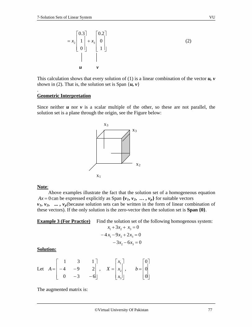
7-Solution Sets of Linear System VU
©Virtual University Of Pakistan 77
2 3
0.3 0.21 00 1
x x = +
(2)
u v This calculation shows that every solution of (1) is a linear combination of the vector u, v shown in (2). That is, the solution set is Span {u, v} . Geometric Interpretation Since neither u nor v is a scalar multiple of the other, so these are not parallel, the solution set is a plane through the origin, see the Figure below: x3
x3
x2 x1 Note: Above examples illustrate the fact that the solution set of a homogeneous equation
0Ax = can be expressed explicitly as Span {v1, v2, … , vp} for suitable vectors v1, v2, ... , vp(because solution sets can be written in the form of linear combination of these vectors). If the only solution is the zero-vector then the solution set is Span {0}. Example 3 (For Practice) Find the solution set of the following homogenous system:
1 2 3
1 2 3
2 3
3 04 9 2 0
3 6 0
x x xx x x
x x
+ + =− − + =
− − =
Solution:
Let 1 3 14 9 20 3 6
A = − − − −
, 1
2
3
xX x
x
=
, 000
b =
The augmented matrix is:

7-Solution Sets of Linear System VU
©Virtual University Of Pakistan 78
1 2
2 3
2 2 1
1 3
2 3
1 3 1 04 9 2 00 3 6 0
1 3 1 0 ~ 0 3 6 0 4 ,
0 3 6 0
1 3 1 00 3 6 00 0 0 0
1 0 5 010 1 2 0 , ( 3)2
0 0 0 0
5 02 0
0 0
R R
R R
R R R
SOx x
x x
− − − − + − −
+
− − +
− =+ =
=
From above results, it is clear that x3 is a free variable, so Ax = 0 has nontrivial solutions (one for each choice of x3). From above equations we have, 1 3 2 35 , 2 ,x x x x= = − with x3 a free variable. As a vector, the general solution of Ax = 0 is given by
1 3
2 3 3 3
3 3
5 5 52 2 , 2
1 1
x xx x x x x v where v
x x
= = − = − = = −
Parametric Vector Form of the solution Whenever a solution set is described explicitly with vectors, we say that the solution is in parametric vector form The equation
x = su + tv (s, t in R) is called a parametric vector equation of the plane. It is written in this form to emphasize that the parameters vary over all real numbers. Similarly, the equation x = x3v (with x3 free), or x = tv (with t in R), is a parametric vector equation of a line.

7-Solution Sets of Linear System VU
©Virtual University Of Pakistan 79
Solutions of Non-homogeneous Systems When a non-homogeneous linear system has many solutions, the general solution can be written in parametric vector form as one vector plus an arbitrary linear combination of vectors that satisfy the corresponding homogeneous system. To clear this concept consider the following examples, Example: 5 Describe all solutions of Ax = b, where
3 5 4 73 2 4 1
6 1 8 4A and b
− = − − = − − −
Solution Row operations on [A b] produce
1 2 1 3
2 3 2
2 1 1
1 3
2
3 5 4 73 2 4 1
6 1 8 4
3 5 4 70 3 0 6 , 20 9 0 18
3 5 4 710 1 0 2 3 ,3
0 0 0 0
41 0 13
10 1 0 2 5 ,3
0 0 0 0
4 13
20 0
R R R R
R R R
R R R
x x
OR x
− − − − − −
− + − + − −
− + − − − +
− = −
==
Thus 1 3 241 , 2,3
x x x= − + = and x3 is free.
As a vector, the general solution of Ax = b has the form

7-Solution Sets of Linear System VU
©Virtual University Of Pakistan 80
3 31
2 3
3 3 3
4 4 41 1 13 3 32 2 0 2 0
0 0 1
x xxx x x
x x x
− + − − = = = + = +
p v The equation x = p + x3v, or, writing t as a general parameter,
x = p + tv (t in R) (3) Note We know that the solution set of this question when Ax = 0 (example 1) has the parametric vector equation x = tv (t in R) (4) With the same v that appears in equation (3) in above example. Thus the solutions of Ax = b are obtained by adding the vector p to the solutions of Ax = 0. The vector p itself is just one particular solution of Ax = b (corresponding to t = 0 in (3)). The following theorem gives the precise statement. Theorem Suppose the equation Ax = b is consistent for some given b, and let p be a solution. Then the solution set of Ax = b is the set of all vectors of the form w = p + vh, where vh is any solution of the homogeneous equation Ax = 0. Example 6: (For practice)
1 2 3
1 2 3
2 3
3 14 9 2 1
3 6 3
x x xx x x
x x
+ + =− − + = −
− − = −
Solution
Let 1 3 14 9 20 3 6
A = − − − −
, 1
2
3
xX x
x
=
, 113
b = − −
The augmented matrix is

7-Solution Sets of Linear System VU
©Virtual University Of Pakistan 81
1 2
2 3
2
2 1
1 3
2 3
1 3 1 14 9 2 10 3 6 3
1 3 1 10 3 6 3 4 ,0 3 6 3
1 3 1 10 3 6 30 0 0 0
1 3 1 110 1 2 13
0 0 0 0
1 0 5 20 1 2 1 ( 3)0 0 0 0
5 22 1
0 0
R R
R R
R
R R
SOx x
x x
− − − − − − + − − − +
− − − +
− = −+ =
=
Thus 1 3 2 32 5 , 1 2 ,x x x x= − + = − and x3 is free. As a vector, the general solution of Ax = b has the form
1 3 3
2 3 3
3 3 3
2 5 2 5 2 51 2 1 2 1 2
0 0 1
x x xx x x x
x x x
− + − − = = − = + − = + −
p v So we can write solution set in parametric vector form as 3x p x v= +
7-Solution Sets of Linear System VU
©Virtual University Of Pakistan 82
Exercise Determine if the system has a nontrivial solution. Try to use as few row operations as possible. 1. x1 – 5x2 + 9x3 = 0 2. 3x1 + 6x2 – 4x3 – x4 = 0 -x1 + 4x2 – 3x3 = 0 -5x1 + 8x3 + 3x4 = 0 2x1 – 8x2 + 9x3 = 0 8x1 – x2 + 7x4 = 0 3. 5x1 – x2 + 3x3 = 0 4x1 – 3x2 + 7x3 = 0 Write the solution set of the given homogeneous system in parametric vector form. 4. x1 – 3x2 – 2x3 = 0 5. x1 + 2x2 – 7x3 = 0 x2 – x3 = 0 -2x1 – 3x2 + 9x3 = 0 -2x1 + 3x2 + 7x3 = 0 –2x2 + 10x3 = 0 In exercises 6-8, describe all solutions of Ax = 0 in parametric vector form where A is row equivalent to the matrix shown.
6.
1 5 0 2 0 40 0 0 1 0 30 0 0 0 1 50 0 0 0 0 0
− − −
7.
1 6 0 8 1 20 0 1 3 4 60 0 0 0 0 10 0 0 0 0 0
− − −
8. [ ]1 5 0 4−
Steps of Writing a Solution Set (of a Consistent System) in a Parametric Vector Form
Step 1: Row reduces the augmented matrix to reduced echelon form. Step 2: Express each basic variable in terms of any free variables appearing in an equation. Step 3: Write a typical solution x as a vector whose entries depend on the free variables if any. Step 4: Decompose x into a linear combination of vectors (with numeric entries) using the free variables as parameters.

7-Solution Sets of Linear System VU
©Virtual University Of Pakistan 83
9. Describe the solution set in R3 of x1 – 4x2 + 3x3 = 0, compare it with the solution set of x1 – 4x2 + 3x3 = 7. 10. Find the parametric equation of the line through a parallel to b.
3 1,
8 5a b
− = = −
11. Find a parametric equation of the line M through p and q.
1 0,
4 7p q
− = =
12. Given5 108 16
7 14A
= − −
, find one nontrivial solution of Ax = 0 by inspection.
13. Given1 32 63 9
A =
, find one nontrivial solution of Ax = 0 by inspection.

8-Linear Independence VU
©Virtual University Of Pakistan 84
Lecture 8
Linear Independence Definition An indexed set of vectors {v1, v2, ... , vp} in Rn is said to be linearly independent if the vector equation 1 1 2 2 0p px v x v x v+ + + = has only the trivial solution. The set {v1, v2, ... , vp} is said to be linearly dependent if there exist weights c1, …. , cp, not all zero, such that 1 1 2 2 0p pc v c v c v+ + + = (1) Equation (1) is called a linear dependence relation among v1 ,…, vp , when the weights are not all zero. Example 1
Let 1 2 3
1 4 22 , 5 , 13 6 0
v v v = = =
(a) Determine whether the set of vectors {v1, v2, v3} is linearly independent or not. (b) If possible, find a linear dependence relation among v1, v2, v3. Solution (a) Row operations on the associated augmented matrix show that
1 2 1 3
2 3
1 4 2 02 5 1 03 6 0 0
1 4 2 00 3 3 0 ( 2) , ( 3)0 6 6 0
1 4 2 00 3 3 0 (2)0 0 0 0
R R R R
R R
− − − + − + − − − − +
Clearly, x1 and x2 are basic variables and x3 is free. Each nonzero value of x3 determines a nontrivial solution. Hence v1, v2, v3 are linearly dependent (and not linearly independent). (b) To find a linear dependence relation among v1, v2, v3, completely row reduce the augmented matrix and write the new system:

8-Linear Independence VU
©Virtual University Of Pakistan 85
2
1 2
1 4 2 010 1 1 0
30 0 0 0
1 0 2 00 1 1 0 40 0 0 0
R
R R
−
− −
⇒ 1 3
2 3
2 00
0 0
x xx x
− =+ =
=
Thus x1 = 2x3, x2 = -x3, and x3 is free. Choose any nonzero value for x3, say, x3 = 5, then x1 = 10, and x2 = -5. Substitute these values into 1 1 2 2 3 3 0x v x v x v+ + = ⇒ 10v1 – 5v2 + 5v3 = 0 This is one (out of infinitely many) possible linear dependence relation among v1, v2, v3. Example (for practice) Check whether the vectors are linearly dependent or linearly independent.
1 2(3, 1) ( 2,2)v v= − = − Solution Consider two constants 1C and 2C . Suppose:
1 2
1 2 1 2
(3, 1) ( 2,2) 0(3 2 , 2 ) (0,0)c c
c c c c− + − =− − + =
Now, set each of the components equal to zero to arrive at the following system of equations:
1 2
1 2
3 2 02 0
c cc c− =
− + =
Solving this system gives the following solution,
1 20 0c c= = The trivial solution is the only solution, so these two vectors are linearly independent.

8-Linear Independence VU
©Virtual University Of Pakistan 86
Linear Independence of Matrix Columns Suppose that we begin with a matrix [ ]1 ... nA a a= instead of a set of vectors. The matrix equation Ax = 0 can be written as 1 1 2 2 0n nx a x a x a+ + + = Each linear dependence relation among the columns of A corresponds to a nontrivial solution of Ax = 0. Thus we have the following important fact. The columns of a matrix A are linearly independent if and only if the equation
0Ax = has only the trivial solution.
Example 2 Determine whether the columns of 0 1 41 2 15 8 0
A = −
are linearly
independent. Solution To study Ax = 0, row reduce the augmented matrix:
12
1 3
0 1 4 01 2 1 05 8 0 0
1 2 1 00 1 4 05 8 0 0
1 2 1 00 1 4 0 ( 5)0 2 5 0
R
R R
−
−
− − + −
2 3
1 2 1 00 1 4 0 (2)0 0 13 0
R R−
+
At this point, it is clear that there are three basic variables and no free variables. So the equation Ax = 0 has only the trivial solution, and the columns of A are linearly independent. Sets of One or Two Vectors A set containing only one vector (say, v) is linearly independent if and only if v is not the zero vector. This is because the vector equation x1v = 0 has only the trivial solution when 0v ≠ . The zero vector is linearly dependent because x10 = 0 has many nontrivial solutions.

8-Linear Independence VU
©Virtual University Of Pakistan 87
Example 3 Check the following sets for linearly independence and dependence.
a. 1 2
3 6,
1 2v v = =
b. 1 2
3 6,
2 2v v = =
Solution a) Notice that v2 is a multiple of v1, namely, v2 = 2v1.
Hence –2v1 + v2 = 0, which shows that {v1, v2} is linearly dependent.
b) v1 and v2 are certainly not multiples of one another. Could they be linearly dependent? Suppose c and d satisfy cv1 + dv2 = 0 If 0,c ≠ then we can solve for v1 in terms of v2, namely, v1 = (-d/c) v2. This result is impossible because v1 is not a multiple of v2. So, c must be zero. Similarly, d must also be zero. Thus {v1, v2} is a linearly independent set.
Note A set of two vectors {v1, v2} is linearly dependent if and only if one of the vectors is a multiple of the other. In geometric terms, two vectors are linearly dependent if and only if they lie on the same line through the origin. Figure 1, shows the vectors from Example 3. x2 (6, 2) (3, 1) x1 Linearly dependent x2 (3, 2) (6, 2) x1

8-Linear Independence VU
©Virtual University Of Pakistan 88
Figure 1 Linearly independent Sets of Two or More Vectors Theorem (Characterization of Linearly dependent Sets) An indexed set 1 2{ , , , }ps v v v= of two or more vectors is linearly dependent if and only if at least one of the vectors in S is a linear combination of the others. In fact, if S is linearly dependent, and 0v ≠ , then some jv (with 1j > ) is a linear combination of the preceding vectors, 1 1, , jv v − . Proof If some jv in S equals a linear combination of the other vectors, then
jv can be subtracted from both sides of the equation, producing a linear dependence relation with a nonzero weight (–1) on jv . For instance, if v1 = c2v2 + c3v3, then 0 = (–1)v1 + c2v2 +c3v3 + 0v4 + ... + 0vp. Thus S is linearly dependent.
Conversely, suppose S is linearly dependent. If v1 is zero, then it is a (trivial) linear combination of the other vectors in S. If 0v ≠ and there exist weights c1, ... , cp, not all zero(because vectors are linearly dependent), such that
c1v1 + c2v2 +…+ cpvp = 0
Let j be the largest subscript for which 0jc ≠ . If 1j = , then c1v1 = 0, which is impossible because 0jv ≠ . So 1j > , and 1 1 10 0 0j j j pc v c v v v++ + + + + =
1 1 2 2 1 1j j j jc v c v c v c v− −= − − − −
11 21 2 1
jj j
j j j
cc cv v v vc c c
−−
= − + − + +
Note: This theorem does not say that every vector in a linearly dependent set is a linear combination of the preceding vectors. A vector in a linearly dependent set may fail to be a linear combination of the other vectors.

8-Linear Independence VU
©Virtual University Of Pakistan 89
Example 4 Let 310
u =
and 160
v =
. Describe the set spanned by u and v, and prove
that a vector w is in Span {u, v} if and only if {u, v, w} is linearly dependent.
Solution The vectors u and v are linearly independent because neither vector is a multiple of the other, nor so they span a plane in R3. In fact, Span {u, v} is the x1x2-plane (with x3 = 0). If w is a linear combination of u and v, then {u, v, w} is linearly dependent. Conversely, suppose that {u, v, w} is linearly dependent. Some vector in {u, v, w} is a linear combination of the preceding vectors (since 0u ≠ ). That vector must be w, since v is not a multiple of u. So w is in Span {u, v} x3 x2 v u x1 w Linearly dependent w in Span {u, v}. x3 w v x2 x1 u Linearly independent w not in Span {u, v}
Figure 2: Linear dependence in R3. This example generalizes to any set {u, v, w} in R3 with u and v linearly independent. The set {u, v, w} will be linearly dependent if and only if w is in the plane spanned by u and v. Theorem If a set contains more vectors than there are entries in each vector, then the set is linearly dependent. That is, any set {v1, v2, ... , vp} in Rn is linearly dependent if p > n.

8-Linear Independence VU
©Virtual University Of Pakistan 90
Example 5 The vectors 2 4 2
, ,1 1 2
− −
are linearly dependent, because there are
three vectors in the set and there are only two entries in each vector. Notice, however, that none of the vectors is a multiple of one of the other vectors. See Figure 4. x2 (–2, 2) (2, 1) x1 (4, –1)
Figure 4 A linearly dependent set in R2.
Theorem If a set S = {v1, v2, … , vp} in Rn contains the zero vector, then the set is linearly dependent. Proof By renumbering the vectors, we may suppose that v1 = 0. Then (1)v1 + 0v2 + … + 0vp = 0 shows that S is linearly dependent( because in this relation coefficient of v1 is non zero). Example 6 Determine by inspection if the given set is linearly dependent.
a. 1 2 3 47 , 0 , 1 , 16 9 5 8
b. 2 0 13 , 0 , 15 0 8
c.
2 34 6
,6 9
10 15
− − −
Solution
a) The set contains four vectors that each has only three entries. So,the set is linearly dependent by the Theorem above.
b) The same theorem does not apply here because the number of vectors does not exceed the number of entries in each vector. Since the zero vector is in the set, the set is linearly dependent by the next theorem.

8-Linear Independence VU
©Virtual University Of Pakistan 91
c) As we compare corresponding entries of the two vectors, the second vector seems to be –3/2 times the first vector. This relation holds for the first three pairs of entries, but fails for the fourth pair. Thus neither of the vectors is a multiple of the other, and hence they are linearly independent.
Exercise
1. Let 3 6 0 32 , 1 , 5 , 74 7 2 5
u v w and z−
= = = − = − −
.
(i) Are the sets {u, v}, {u, w}, {u, z}, {v, w}, {v, z}, and {w, z} each linearly
independent? Why or why not? (ii) Does the answer to Problem (i) imply that {u, v, w, z} is linearly independent?
(iii) To determine if {u, v, w, z} is linearly dependent, is it wise to check if, say w is a linear combination of u, v and z?
(iv) Is {u, v, w, z} linear dependent? Decide if the vectors are linearly independent. Give a reason for each answer.
2. 3 3 60 , 2 , 40 3 0
−
3. 1 3 03 , 5 , 5
2 6 6
− − − −
Determine if the columns of the given matrix form a linearly dependent set.
4. 1 3 2 03 10 7 15 5 3 7
− − − −
5.
3 4 31 7 7
1 3 20 2 6
− − − −
6.
1 1 0 41 0 3 1
0 2 1 11 0 1 3
− − − −
7.
1 1 3 00 1 5 41 2 8 5
3 1 1 3
− − − −
For what values of h is v3 in span {v1, v2} and for what values of h is {v1, v2, v3} linearly dependent?
8. 1 2 3
1 2 13 , 6 , 2
2 4v v v
h
− = = − = −
9. 1 2 3
1 3 23 , 9 , 63 1
v v vh
− = = = − −

8-Linear Independence VU
©Virtual University Of Pakistan 92
Find the value(s) of h for which the vectors are linearly dependent.
10. 1 2 13 , 4 , 1
3 1 h
− − − −
11. 1 3 4
5 , 8 ,2 6 8
h−
− − −
Determine by inspection whether the vectors are linearly independent. Give reasons for your answers.
12. 5 6 2 3
, , ,5 1 4 6 −
13. 2 6 0
5 , 5 , 01 3 0
− −
14. 6 32 , 1
8 2
− −
15. Given
2 3 55 1 43 1 4
1 0 1
A
− − = − − −
, observe that the third column is the sum of the first two
columns. Find a nontrivial solution of Ax = 0 without performing row operations. Each statement in exercises 16-18 is either true(in all cases) or false(for at least one example). If false, construct a specific example to show that the statement is not always true. If true, give a justification. 16. If v1, …, v4 are in R4, and v3 = 2v1 + v2, then {v1, v2, v3, v4} is linearly dependent. 17. If v1 and v2 are in R4, and v1 is not a scalar multiple of v2, then {v1, v2} is linearly independent. 18. . If v1, …, v4 are in R4, and{v1, v2, v3} is linearly dependent, then {v1, v2, v3, v4} is also linearly dependent.
19. Use as many columns of
8 3 0 7 29 4 5 11 7
6 2 2 4 45 1 7 0 10
A
− − − − = − − −
as possible to construct a
matrix B with the property that equation Bx = 0 has only the trivial solution. Solve

8-Linear Independence VU
©Virtual University Of Pakistan 93
Bx = 0 to verify your work.

9-Linear Transformations VU
©Virtual University Of Pakistan 94
Lecture 9
Linear Transformations
Outlines
• Matrix Equation • Transformation, Examples, Matrix as Transformations • Linear Transformation, Examples, Some Properties
Matrix Equation An equation Ax = b is called a matrix equation in which a matrix A acts on a vector x by multiplication to produce a new vector called b. For instance, the equations
14 3 1 3 1 52 0 5 1 1 8
1
14 3 1 3 4 02 0 5 1 1 0
3
A x band
A u o
− =
− = −
Solution of Matrix Equation Solution of the Ax = b consists of those vectors x in the domain that are transformed into the vector b in range. Matrix equation Ax = b is an important example of transformation we would see later in the lecture. Transformation or Function or Mapping

9-Linear Transformations VU
©Virtual University Of Pakistan 95
A transformation (or function or mapping) T from R n to R m is a rule that assigns to each vector x in Rn, an image vector T(x) in Rm. : n mT R R→ The set R n is called the domain of T, and R m is called the co-domain of T. For x in Rn the set of all images T(x) is called the range of T. Note To define a mapping or function, domain and co-domain are the ordinary sets. However to define a linear transformation, the domain and co-domain has to be
( )m nor . Moreover a map : m nT → is a linear transformation if for any two vectors say , mu v∈ and the scalars 1 2,c c , the following equation is satisfied ( )1 2 1 2( ) ( )T c u c v c T u c T v+ = +
Example1 Consider a mapping 2 2:T R R→ defined by ( , ) ( , )T x y x y= − . This transformation is a reflection about y-axis in xy plane. Here (1,2) ( 1,2)T = − . T has transformed vector (1,2) into another vector (-1,2). In matrix form:
1 00 1
x xTv Av
y y− −
= = =
y (-x, y) <------------------------------------------ (x, y) x Further the projection transformation 2 2:T R R→ defined by ( , ) ( ,0)T x y x= is given as:
1 00 0 0
x xTv Av
y
= = =
Example 2 Let 1 3 3 3
23 5 , , 2 , 2
11 7 5 5
A u b c−
= = = = − − −
,

9-Linear Transformations VU
©Virtual University Of Pakistan 96
and define a transformation 2 3:T R R→ by T(x) = Ax, so that
1 21
1 22
1 2
1 3 3( ) 3 5 3 5
1 7 7
x xx
T x Ax x xx
x x
− − = = = + − − +
a) Find T (u), the image of u under the transformation T. b) Find an x in R2, whose image under T is b. c) Is there more than one x whose image under T is b? d) Determine if c is in the range of the transformation T.
Solution (a)
1 3 5
2( ) 3 5 1
11 7 9
T u Au−
= = = − − −
Here 5
( ) 19
T u = −
Here the matrix transformation has transformed 21
u = −
into another vector 519
−
(b) We have to find an x such that T (x) = b or Ax = b
i. e 1
2
1 3 33 5 21 7 5
xx
− = − −
(1)
Now row reduced augmented matrix will be:
9-Linear Transformations VU
©Virtual University Of Pakistan 97
1 2 1 3
2 2 3
2 1
1 3 33 5 2 3 ,1 7 5
1 3 310 14 7 , 4 ,
140 4 2
1 3 30 1 .5 30 0 0
1 0 1.50 1 .50 0 0
R R R R
R R R
R R
− − + + − −
− − − + −
− − + −
Hence x1 = 1.5, x2 = - 0.5, and 1.5
..5
x = −
The image of this x under T is the given vector b. (c) From (2) it is clear that equation (1) has a unique solution. So, there is exactly one x whose image is b. (d) The vector c is in the range of T if c is the image of some x in R2, that is, if
( )c T x= for some x. This is just another way of asking if the system Ax = c is consistent. To find the answer, we will row reduce the augmented matrix:
1 2 1 3
3 23
2 3
1 3 33 5 2 3 ,1 7 5
1 3 310 14 7 ,4
0 4 8
1 3 30 1 2 140 14 7
1 3 30 1 20 0 35
R R R R
R R
R R
− − + + −
− −
− − + −
− −

9-Linear Transformations VU
©Virtual University Of Pakistan 98
1 2
1 2
1 2
3 30 20 0 35 0 35 0 35
x xx xx x but
− =+ =+ = − ⇒ = ≠
Hence the system is inconsistent. So c is not in the range of T. So from the above example we can view a transformation in the form of a matrix. We’ll see that a transformation : n mT R R→ can be transformed into a matrix of order m n× and every matrix of order m n× can be viewed as a linear transformation. The next two matrix transformations can be viewed geometrically. They reinforce the dynamic view of a matrix as something that transforms vectors into other vectors.
Example 3 If 1 0 00 1 0 ,0 0 0
A =
then the transformation x Ax→ projects points in R3
onto the 1 2x x coordinate plane− because 1 1 1
2 2 2
3 3
1 0 00 1 00 0 0 0
x x xx x xx x
→ =
x3
• • • • x2 • • x1 • • A projection transformation
Example 4 Let 1 3
.0 1
A =
, the transformation 2 2:T R R→ defined by T (x) = Ax is
called a shear transformation.
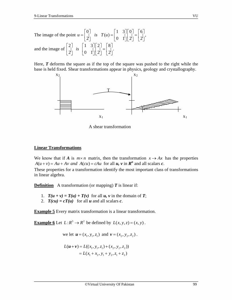
9-Linear Transformations VU
©Virtual University Of Pakistan 99
The image of the point 0 1 3 0 6
( ) ,2 0 1 2 2
u is T u = = =
and the image of 2 1 3 2 8
.2 0 1 2 2
is =
Here, T deforms the square as if the top of the square was pushed to the right while the base is held fixed. Shear transformations appear in physics, geology and crystallography. x2 x2 T x1 x1
A shear transformation Linear Transformations We know that if A is m n× matrix, then the transformation x Ax→ has the properties
( ) ( )A u v Au Av and A cu cAu+ = + = for all u, v in Rn and all scalars c. These properties for a transformation identify the most important class of transformations in linear algebra. Definition A transformation (or mapping) T is linear if:
1. T(u + v) = T(u) + T(v) for all u, v in the domain of T; 2. T(cu) = cT(u) for all u and all scalars c.
Example 5 Every matrix transformation is a linear transformation. Example 6 Let 3 2:L R R→ be defined by ( , , ) ( , )L x y z x y= . we let 1 1 1( , , )x y z=u and 2 2 2( , , )x y z=v .
1 1 1 2 2 2
1 2 1 2 1 2
( ) (( , , ) ( , , ))( , , )
L L x y z x y zL x x y y z z
+ = += + + +
u v

9-Linear Transformations VU
©Virtual University Of Pakistan 100
1 2 1 2
1 1 2 2
( , )( , ) ( , ) ( ) ( )x x y yx y x y L L
= + += + = +u v
Also, if k is a real number, then 1 1 1 1 1( ) ( , , ) ( , ) ( )L k L kx ky kz kx ky kL= = =u u Hence, L is a linear transformation, which is called a projection. The image of the vector (or point) (3, 5, 7) is the vector (or point) (3, 5) in xy-plane. See figure below: z (3, 5, 7) y (3, 5) x Geometrically the image under L of a vector (a, b, c) in R3 is (a, b) in R2 can be found by drawing a line through the end point P(a, b, c) of u and perpendicular to R2, the xy-plane. The intersection Q(a, b)of this line with the xy-plane will give the image under L. See the figure below: Q(a, b) v = L(u) P(a, b)
9-Linear Transformations VU
©Virtual University Of Pakistan 101
Example 7 Let :L R R→ be defined by 2( )L x x= Let x and y in R and
2 2 2 2 2( ) ( ) 2 ( ) ( )
( ) ( ) ( )L x y x y x y xy x y L x L y
L x y L x L y+ = + = + + ≠ + = +
⇒ + ≠ +
So we conclude that the function L is not a linear transformation. Linear transformations preserve the operations of vector addition and scalar multiplication. Properties If T is a linear transformation, then
1. T(0) = 0 2. T(cu +dv) = cT(u) + dT(v) 3. T(c1v1 + …+ cpvp) = c1T(v1) + … + cpT(vp)
for all vectors u, v in the domain of T and all scalars c, d. Proof 1. By the definition of Linear Transformation we have T(cu) = cT(u) for all u and all scalars c. Put 0c = we’ll get T(0u)= 0T(u) This implies T(0) = 0 2. Just apply the definition of linear transformation. i. e
T(cu + dv) = T(cu) + T(dv) = cT(u) + dT(v)
Property (3) follows from (ii), because T(0) = T (0u) =0T(u) = 0. Property (4) requires both (i) and (ii): OBSERVATION Observe that if a transformation satisfies property 2 for all u, v and c, d, it must be linear (Take c = d = 1 for preservation of addition, and take d = 0)
9-Linear Transformations VU
©Virtual University Of Pakistan 102
3. Generalizing Property 2 we’ll get 3
T(c1v1 + …+ cpvp) = c1T(v1) + … + cpT(vp) Applications in Engineering In engineering and physics, property 3 is referred to as a superposition principle. Think of v1, … , vp as signals that go into a system or process and T(v1), … , T(vp) as the responses of that system to the signals. The system satisfies the superposition principle if an input is expressed as a linear combination of such signals, the system’s response is the same linear combination of the responses to the individual signals. Example 8 Given a scalar r, define :T R R→ by T (x) = x+1. T is not a linear transformation (why!) because (0) 0T ≠ (by property 3) Example 9 Given a scalar r, define 2 2:T R R→ by T (x) = rx. T is called a contraction when 0 1r≤ < and a dilation when 1.r ≥ Let r = 3 and show that T is a linear transformation. Solution Let u, v be in R2 and let c, d be scalars, then T (cu + dv) = 3 (cu + dv) Definition of T = 3cu + 3dv = c (3u) + d(3v) Vector arithmetic = cT (u) + dT (v) Thus T is a linear transformation because it satisfies (4). Example 10 Define a linear transformation 2 2:T R R→ by
1 2
2 1
0 1( )
1 0x x
T xx x
−− = =
Find the images under T of 4 2 6
, , .1 3 4
u v and u v = = + =

9-Linear Transformations VU
©Virtual University Of Pakistan 103
Solution 0 1 4 1 0 1 2 3
( ) , ( )1 0 1 4 1 0 3 2
T u T v− − − −
= = = =
0 1 6 4
( )1 0 4 6
T u v− −
+ = =
In the above example, T rotates u, v and u + v counterclockwise through 900. In fact, T transforms the entire parallelogram determined by u and v into the one determined by T (u) and T (v) Example 11 Let L: R3→R2 be a linear transformation for which:
L (1, 0, 0) = (2, -1), L (0, 1, 0) = (3, 1), and L (0, 0, 1) = (-1, 2).
Then find L (-3, 4, 2). Solution Since (-3, 4, 2) = -3i + 4j + 2k,
( 3, 4, 2) ( 3 4 2 ) 3 ( ) 4 ( ) 2 ( )
3(2, 1) 4(3,1) 2( 1,2) (4,11)L L L L L− = − + + = − + +
=− − + + − =i j k i j k
Exercise 1. Suppose that 5 2:T R R→ and T(x) = Ax for some matrix A and each x in R5. How
many rows and columns do A have?
2. Let 1 00 1
A = −
. Give a geometric description of the transformation x Ax→ .
3. The line segment from 0 to a vector u is the set of points of the form tu, where
0 1t≤ ≤ . Show that a linear transformation T maps this segment into the segment between 0 and T(u).
4. Let 2 0 0 1 50 2 0 , 0 , 10 0 2 3 4
A u and = = − −
. Define T:R3→R3 by T (x) = Ax. Find T (u)
and T (v). In exercises 5 and 6, with T defined by T (x) = Ax, find an x whose image under T is b, and determine if x is unique.

9-Linear Transformations VU
©Virtual University Of Pakistan 104
5. 1 0 1 03 1 5 , 54 2 1 6
A b−
= − = − − −
6.
1 0 3 10 1 4 5
,3 2 1 72 1 2 3
b
− − = − − − −
Find all x in R4 that are mapped into the zero vector by the transformation x→Ax.
7.
1 2 7 50 1 4 01 0 1 62 1 6 8
A
− − = −
8. 1 3 4 30 1 3 23 7 6 5
− − −
9. Let 1
17
b = −
and let A be the matrix in exercise 8. Is b in the range of the linear
transformation x→Ax?
10. Let
950
9
b
= −
and let A be the matrix in exercise 7. Is b in the range of the linear
transformation x→Ax? Let T (x) = Ax for x in R2.
(a) On a rectangular coordinate system, plot the vectors u, v, T (u) and T (v). (b) Give a geometric description of what T does to a vector x in R2.
11. 1 0 5 3
, ,0 1 2 1
A u and v−
= = = − − 12.
.5 0 4 5, ,
0 .5 2 2A u and v
− = = = −
13. Let T: R2→R2 be a linear transformation that maps
1 3 1.
5 1 42
u into and maps v into 0
= = −
Use the fact that T is linear find the images
under T of 2u, 3v, and 2u + 3v.

9-Linear Transformations VU
©Virtual University Of Pakistan 105
14. Let 1 2 1 2
1 0 3 2, , , .
0 1 5 7e e y and y
− = = = = −
Let T: R2→R2 be a linear
transformation that maps e1 into y1 and maps e2 into y2. Find the images of 1
2
7.
6x
andx
15. Let 11 2
2
7 3, .
4 8x
x v and vx
− = = = −
Let T: R2→R2 be a linear transformation that
maps x into 1 1 2 2x v x v+ . Find a matrix A such that T (x) is Ax for each x.

10- The Matrix of a Linear Transformation VU
©Virtual University Of Pakistan 106
Lecture 10
The Matrix of a Linear Transformation Outline
• Matrix of a Linear Transformation. • Examples, Geometry of Transformation, Reflection and Rotation • Existence and Uniqueness of solution of T(x)=0
In the last lecture we discussed that every linear transformation from Rn to Rm is actually a matrix transformation x Ax→ , where A is a matrix of order m n× . First see an example
Example 1 The columns of 2
1 00 1
I =
are 1
10
e =
and 2
01
e =
.
Suppose T is a linear transformation from R2 into R3 such that
1 2
5 3( ) 7 ( ) 8
2 0T e and T e
− = − =
with no additional information, find a formula for the image of an arbitrary x in R2.
Solution Let 11 2 1 1 2 2
2
1 00 1
xx x x x e x e
x
= = + = +
Since T is a linear transformation, 1 1 2 2( ) ( ) ( )T x x T e x T e= +
1 2
1 2 1 2
1
1 2
1 2
1
5 3 5 3( ) 7 8 7 8
2 0 2 0
5 3( ) 7 8
2 0
x xT x x x x x
x
x xHence T x x x
x
− − = − + = − + +
− = − + +
Theorem Let : n mT R R→ be a linear transformation. Then there exists a unique matrix A such that ( )T x Ax= for all x in Rn

10- The Matrix of a Linear Transformation VU
©Virtual University Of Pakistan 107
In fact, A is the m n× matrix whose jth column is the vector T (ej), where je is the jth column of the identity matrix in Rn.
[ ]1( ) ... ( )nA T e T e=
Proof Write
[ ] [ ]
1 1
2 21 2
1
21 1 1 1
0 0 1 0 00 0 0 1 0
... ...
0 0 0 10
... ... ...
n
nn
n n n n
n
x xx x
x x x x
xx
xx
x e x e e e e e x
x
= = + + + = + + +
= + + = =
Since T is Linear, So
1 1 1 1( ) ( ... ) ( ) ... ( )n n n nT x T x e x e x T e x T e= + + = + +
[ ]1
1( ) ... ( )n
n
xT e T e Ax
x
= =
(1)
The matrix A in (1) is called the standard matrix for the linear transformation T. We know that every linear transformation from Rn to Rm is a matrix transformation and vice versa. The term linear transformation focuses on a property of a mapping, while matrix transformation describes how such a mapping is implemented, as the next three examples illustrate. Example 2 Find the standard matrix A for the dilation transformation T (x) = 3x, 2x R∈ . Solution Write
1 1 2 2
3 0( ) 3 ( ) 3
0 3T e e and T e e
= = = =
3 00 3
A =

10- The Matrix of a Linear Transformation VU
©Virtual University Of Pakistan 108
Example 3 Let 3 3:L R R→ is the linear operator defined byx x y
L y y zz x z
+ = − +
.
Find the standard matrix representing L and verify L (x) = Ax. Solution The standard matrix A representing L is the 3 x 3 matrix whose columns are L (e1), L (e2), and L (e3) respectively. Thus
1 1
1 1 0 1( ) 0 0 0 0 ( )
0 1 0 1L e L col A
+ = = − = = +
2 2
0 0 1 1( ) 1 1 0 1 ( )
0 0 0 0L e L col A
+ = = − = = +
3 3
0 0 0 0( ) 0 0 1 1 ( )
1 0 1 1L e L col A
+ = = − = − = +
Hence 1 1 00 1 11 0 1
A = −
Now Ax = 1 1 00 1 1 ( )1 0 1
x x yy y z L xz x z
+ − = − = +
Hence verified. Example 4 Let 2 2:T R R→ be the transformation that rotates each point in R2 through an angleϕ , with counterclockwise rotation for a positive angle. We could show geometrically that such a transformation is linear. Find the standard matrix A of this transformation.
Solution 10
rotates into cos
,sin
ϕϕ
and 01
rotates into sin
.cos
ϕϕ
−
See figure below.

10- The Matrix of a Linear Transformation VU
©Virtual University Of Pakistan 109
By above theorem cos sinsin cos
Aϕ ϕϕ ϕ
− =
A rotation transformation Example 5 A reflection with respect to the x-axis of a vector u in R2 is defined by the
linear operator 1 1
2 2
( )a a
L u La a
= = −
.
Then 1
1 1( )
0 0L e L
= =
and 2
0 0( )
1 1L e L
= = −
Hence the standard matrix representing L is 1 00 1
A = −
Thus we have 1 1
2 2
1 0( )
0 1a a
L u Aua a
= = = − −
To illustrate a reflection with respect to the x-axis in computer graphics, let the triangle T have vertices (-1, 4), (3, 1), and (2, 6).
To reflect T with respect to x-axis, we let 1 2 3
1 3 2, ,
4 1 6u u u
− = = =
and compute the
images L (u1), L (u2), and L (u3) by forming the products

10- The Matrix of a Linear Transformation VU
©Virtual University Of Pakistan 110
1
2
3
1 0 1 1,
0 1 4 4
1 0 3 3,
0 1 1 1
1 0 2 2.
0 1 6 6
Au
Au
Au
− − = = − −
= = − −
= = − −
Thus the image of T has vertices (-1, -4), (3, -1), and (2, -6). Geometric Linear Transformations of R2 Examples 3-5 illustrate linear transformations that are described geometrically. In example 4 transformations is a rotation in the plane. It rotates each point in the plane through an angleϕ . Example 5 is reflection in the plane. Existence and Uniqueness of the solution of T(x)=b The concept of a linear transformation provides a new way to understand existence and uniqueness questions asked earlier. The following two definitions give the appropriate terminology for transformations. Definition A mapping : n mT R R→ is said to be onto Rm if each b in Rm is the image of at least one x in Rn.
OR Equivalently, T is onto Rm if for each b in Rm there exists at least one solution of T (x) = b. “Does T map Rn onto Rm?” is an existence question. The mapping T is not onto when there is some b in Rm such that the equation T (x) = b has no solution. Definition A mapping : n mT R R→ is said to be one-to-one (or 1:1) if each b in Rm is the image of at most one x in Rn.

10- The Matrix of a Linear Transformation VU
©Virtual University Of Pakistan 111
OR Equivalently, T is one-to-one if for each b in Rm the equation T (x) = b has either a unique solution or none at all, “Is T one-to-one?” is a uniqueness question. The mapping T is not one-to-one when some b in Rm is the image of more than one vector in Rn. If there is no such b, then T is one-to-one. Example 6 Let T be the linear transformation whose standard matrix is
1 4 8 10 2 1 30 0 0 5
A−
= −
Does T map R4 onto R3? Is T a one-to-one mapping?
Solution Since A happens to be in echelon form, we can see at once that A has a pivot position in each row. We know that for each b in R3, the equation Ax = b is consistent. In other words, the linear transformation T maps R4 (its domain) onto R3. However, since the equation Ax = b has a free variable (because there are four variables and only three basic variables), each b is the image of more than one x. That is, T is not one-to-one. Theorem Let : n mT R R→ be a linear transformation. Then T is one-to-one if and only if the equation T (x) = 0 has only the trivial solution. Proof: Since T is linear, T (0) = 0 if T is one-to-one, then the equation T (x) = 0 has at most one solution and hence only the trivial solution. If T is not one-to-one, then there is a b that is the image of at least two different vectors in Rn (say, u and v). That is, T (u) = b and T (v) = b. But then, since T is linear ( ) ( ) 0T u v T u b b− = = − = The vector u – v is not zero, since u v≠ . Hence the equation T (x) = 0 has more than one solution. So either the two conditions in the theorem are both true or they are both false. Kernel of a Linear Transformation Let :T V W→ be a linear transformation. Then kernel of T (usually written as KerT), is the set of those elements in V which maps onto the zero vector in W .Mathematically: { }| ( ) 0KerT v V T v in W= ∈ =
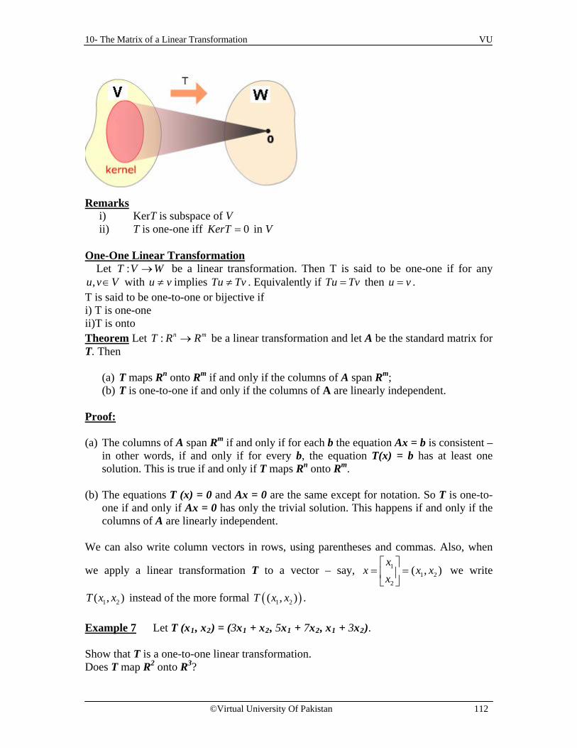
10- The Matrix of a Linear Transformation VU
©Virtual University Of Pakistan 112
Remarks
i) KerT is subspace of V ii) T is one-one iff 0KerT = in V
One-One Linear Transformation Let :T V W→ be a linear transformation. Then T is said to be one-one if for any
,u v V∈ with u v≠ implies Tu Tv≠ . Equivalently if Tu Tv= then u v= . T is said to be one-to-one or bijective if i) T is one-one ii)T is onto Theorem Let : n mT R R→ be a linear transformation and let A be the standard matrix for T. Then
(a) T maps Rn onto Rm if and only if the columns of A span Rm; (b) T is one-to-one if and only if the columns of A are linearly independent.
Proof: (a) The columns of A span Rm if and only if for each b the equation Ax = b is consistent –
in other words, if and only if for every b, the equation T(x) = b has at least one solution. This is true if and only if T maps Rn onto Rm.
(b) The equations T (x) = 0 and Ax = 0 are the same except for notation. So T is one-to-
one if and only if Ax = 0 has only the trivial solution. This happens if and only if the columns of A are linearly independent.
We can also write column vectors in rows, using parentheses and commas. Also, when
we apply a linear transformation T to a vector – say, 11 2
2
( , )x
x x xx
= =
we write
1 2( , )T x x instead of the more formal ( )1 2( , )T x x . Example 7 Let T (x1, x2) = (3x1 + x2, 5x1 + 7x2, x1 + 3x2). Show that T is a one-to-one linear transformation. Does T map R2 onto R3?

10- The Matrix of a Linear Transformation VU
©Virtual University Of Pakistan 113
Solution When x and T (x) are written as column vectors, it is easy to see that T is described by the equation
1 21
1 22
1 2
3 1 35 7 5 71 3 3
x xx
x xx
x x
+ = + +
(4)
so T is indeed a linear transformation, with its standard matrix A shown in (4). The columns of A are linearly independent because they are not multiples. Hence T is one-to-one. To decide if T is onto R3, we examine the span of the columns of A. Since A is 3 2× , the columns of A span R3 if and only if A has 3 pivot positions. This is impossible, since A has only 2 columns. So the columns of A do not span R3 and the associated linear transformation is not onto R3.

10- The Matrix of a Linear Transformation VU
©Virtual University Of Pakistan 114
Exercises 1. Let 2 2:T R R→ be transformation that first performs a horizontal shear that maps
2e into 2 1.5e e− (but leaves 1e unchanged) and then reflects the result in the x2 – axis. Assuming that T is linear, find its standard matrix. Assume that T is a linear transformation. Find the standard matrix of T. 2. 2 3: , (1,0) (4, 1,2) (0,1) ( 5,3, 6)T R R T and T→ = − = − − 3. 3 2
1 2 3: , ( ) (1, 4), ( ) ( 2,9), ( ) (3, 8),T R R T e T e and T e→ = = − = − where e1, e2, and e3 are the columns of the identity matrix. 4. 2 2:T R R→ rotates points clockwise through π radians. 5. 2 2:T R R→ is a “vertical shear” transformation that maps e1 into e1 + 2e2 but leaves the vector e2 unchanged. 6. 2 2:T R R→ is a “horizontal shear” transformation that maps e2 into e2 – 3e1 but leaves the vector e1 unchanged. 7. 3 3:T R R→ projects each point (x1, x2, x3) vertically onto the x1x2-plane (where x3=0). 8. 2 2:T R R→ first performs a vertical shear mapping e1 into e1 – 3e2(leaving e2 unchanged) and then reflects the result in the x2-axis. 9. 2 2:T R R→ first rotates points counterclockwise through π /4 radians and then reflects the result in the x2-axis. Show that T is a linear transformation by finding a matrix that implements the mapping. Note that x1, x2, … are not vectors but are entries in vectors. 10. 1 2 3 4 1 2 2 3 3 4( , , , ) ( , , ,0)T x x x x x x x x x x= + + + 11. 1 2 3 2 3 1 2 3( , , ) (3 , 4 )T x x x x x x x x= − + + 12. 1 2 3 4 1 2 4( , , , ) 3 4 8T x x x x x x x= − + 13. Let 2 2:T R R→ be a linear transformation such that 1 2 1 2 1 2( , ) ( , 4 7 )T x x x x x x= + + . Find x such that T (x) =(-2, -5).

10- The Matrix of a Linear Transformation VU
©Virtual University Of Pakistan 115
13. Let 2 3:T R R→ be a linear transformation such that 1 2 1 2 1 2 1 2( , ) ( 2 , 3 , 3 2 )T x x x x x x x x= + − − − − . Find x such that T (x) =(-4, 7, 0).
In exercises 14 and 15, let T be the linear transformation whose standard matrix is given. 14. Decide if T is one-to-one mapping. Justify your answer.
5 10 5 48 3 4 74 9 5 33 2 5 4
− − − − − − −
15. Decide if T maps R5 onto R5. Justify your answer.
4 7 3 7 56 8 5 12 87 10 8 9 14
3 5 4 2 65 6 6 7 3
− − − − − − − − − − −

11- Matrix Operations VU
©Virtual University Of Pakistan 116
Lecture 11
Matrix Operations (i-j)th Element of a matrix Let A be an m n× matrix, where m and n are number of rows and number of columns respectively, then ija represents the i-th row and j-th column entry of the matrix. For example 12a represents 1st row and 2nd column entry. Similarly 32a represents 3rd row and 2nd column entry. The columns of A are vectors in Rm and are denoted by (boldface) .1 2 n, , ,a a a
These columns are [ ]...A = 1 2 na a a The number ija is the i-th entry (from the top) of j-th column vector ja .
11 1 1
1
1
... ...
... ...
... ...
j n
i ij in
m mj mn
Columnj
a a a
a a aRow i A
a a a
=
↑ ↑ ↑
1 j na a a
Figure 1 Matrix notation. Definitions A diagonal matrix is a square matrix whose non-diagonal entries are zero.
11
22
0 00 0
0 0 nn
dd
D
d
=
The diagonal entries in ijA a = are 11 22 33, , ,a a a and they form the main diagonal of A.

11- Matrix Operations VU
©Virtual University Of Pakistan 117
For example
1 0 0 02 0 0
5 0 0 0 0 00 3 0
0 7 0 0 16 00 0 11
0 0 0 0
are all diagonal
matrices. Null Matrix or Zero Matrix An m n× matrix whose entries are all zero is a Null or zero matrix and is always written as O. A null matrix may be of any order.
For example
0 0 0 0 00 0 0 0 0
0 0 0 0 00 0 0 0 0
0 0 0 0 00 0 0 0 0
0 0 0 0 0
3 x 3 3 x 2 4 x 5 are all Zero Matrices Equal Matrices Two matrices are said to be equal if they have the same size (i.e., the same number of rows and columns) and same corresponding entries. Example 1 Consider the matrices
2 1 2 1 2 1 0
, ,3 1 3 5 3 4 0
A B Cx
= = = +
The matrices A and B are equal if and only if x+1 = 5 or x = 4. There is no value of x for which A = C, since A and C have different sizes. If A and B are m n× matrices, then the sum, A + B, is the m n× matrix whose columns are the sums of the corresponding columns in A and B. Each entry in A + B is the sum of the corresponding entries in A and B. The sum A + B is defined only when A and B are of the same size. If r is a scalar and A is a matrix, then the scalar multiple rA is the matrix whose columns are r times the corresponding columns in A. Note: Negative of a matrix A is defined as – A to mean (–1)A and the difference of A and B is written as A–B, which means A + (–1) B.
Example 2 Let 4 0 5 1 1 1 2 3
, ,1 3 2 3 5 7 0 1
A B C−
= = = −
Then 5 1 62 8 9
A B + =

11- Matrix Operations VU
©Virtual University Of Pakistan 118
But A + C is not defined because A and C have different sizes. 1 1 1 2 2 2
2 23 5 7 6 10 14
B = =
4 0 5 2 2 2 2 2 32
1 3 2 6 10 14 7 7 12A B
− − = − = − − − −
Theorem 1 Let A, B, and C are matrices of the same size, and let r and s are scalars.
a. A + B = B + A d. r (A + B)= r A + r B b. (A + B) + C = A + (B + C) e. (r + s) A = r A + s A c. A + 0 = A f. r (sA) = (rs) A Each equality in Theorem 1 can be verified by showing that the matrix on the left side has the same size as the matrix on the right and that corresponding columns are equal. Size is no problem because A, B, and C are equal in size. The equality of columns follows immediately from analogous properties of vectors. For instance, if the jth columns of A, B, and C are ,j ja b and jc , respectively, then the jth columns of (A + B) + C and A + (B + C) are
( ) ( )j j j j j ja b c and a b c+ + + + respectively. Since these two vector sums are equal for each j, property (b) is verified. Because of the associative property of addition, we can simply write A + B + C for the sum, which can be computed either as (A + B) + C or A + (B + C). The same applies to sums of four or more matrices. Matrix Multiplication Multiplying an m×n matrix with an n×p matrix results in an m×p matrix. If many matrices are multiplied together, and their dimensions are written in a list in order, e.g. m×n, n×p, p×q, q×r, the size of the result is given by the first and the last numbers (m×r). It is important to keep in mind that this definition requires the number of columns of the first factor A to be the same as the number of rows of the second factor B. When this condition is satisfied, the sizes of A and B are said to conform for the product AB. If the sizes of A and B do not conform for the product AB, then this product is undefined. Definition If A is an m n× matrix, and if B is an n p× matrix with columns 1, , pb b , then the product AB is the m p× matrix whose columns are 1, , pAb Ab .
That is 1 2 1 2... ...p pAB A b b b Ab Ab Ab = =

11- Matrix Operations VU
©Virtual University Of Pakistan 119
This definition makes equation (1) true for all x in Rp. Equation (1) proves that the composite mapping (AB) is a linear transformation and that its standard matrix is AB. Multiplication of matrices corresponds to composition of linear transformations. A convenient way to determine whether A and B conform for the product AB and, if so, to find the size of the product is to write the sizes of the factors side by side as in Figure below (the size of the first factor on the left and the size of the second factor on the right).
A B = AB m x s s x n m x n Inside Outside
If the inside numbers are the same, then the product AB is defined and the outside numbers then give the size of the product.
Example 3 Compute AB, where2 3 4 3 61 5 1 2 3
A and B = = − −
Solution: Here B = [b1 b2 b3], therefore
1 2 3
2 3 4 2 3 3 2 3 6, ,
1 5 1 1 5 2 1 5 3Ab Ab Ab
= = = − − − −
11
1
= −
013
=
219
= −
Then
1 2 3
11 0 21[ ]
1 13 9AB A b b b
= = − −
Ab1 Ab2 Ab3
Note from the definition of AB that its first column, Ab1, is a linear combination of the columns of A, using the entries in b1 as weights. The same holds true for each column of AB. Each column of AB is a linear combination of the columns of A using weights from the corresponding column of B.

11- Matrix Operations VU
©Virtual University Of Pakistan 120
Example 4 Find the product AB for
4 1 4 31 2 4
A = and B = 0 -1 3 12 6 0
2 7 5 2
Solution It follows from definition that the product AB is formed in a column-by-column manner by multiplying the successive columns of B by A. The computations are
1 2 3
1 2 3
c c c4
1 2 4 1 2 4 120 = 4c + 0c + 2c = (4) + (0) + (2) =
2 6 0 2 6 0 82
Similarly, 1
1 2 4 1 2 4 27= -1 = (1) + (-1) + (7) =
2 6 0 2 6 0 -47
4
1 2 4 1 2 4 30= 3 = (4) + (3) + (5) =
2 6 0 2 6 0 265
3
1 2 4 1 2 4 13= 1 = (3) + (1) + (2) =
2 6 0 2 6 0 122
Thus, 4 1 4 3
1 2 4 12 27 30 13= 0 -1 3 1 =
2 6 0 8 -4 26 122 7 5 2
AB
Example 5 (An Undefined Product) Find the product BA for the matrices
4 1 4 31 2 4
0 1 3 12 6 0
2 7 5 2A and B
= = −
Solution The number of columns of B is not equal to number of rows of A so BA multiplication is not possible. The matrix B has size 3 4× and the matrix A has size 2 3× . The “inside” numbers are not the same, so the product BA is undefined. Obviously, the number of columns of A must match the number of rows in B in order for a linear combination such as Ab1 to be defined. Also, the definition of AB shows that AB has the same number of rows as A and the same number of columns as B.

11- Matrix Operations VU
©Virtual University Of Pakistan 121
Example 6 If A is a 3 5× matrix and B is a 5 2× matrix, what are the sizes of AB and BA, if they are defined? Solution The product of matrices A and B of orders 3 5× and 5 2× will result in 3 2× matrix AB. But for BA we have 5 2× and 3 5× , here number of columns in1st matrix are 2 which is not equal to number of rows in 2nd matrix. So BA is not possible. Since A has 5 columns and B has 5 rows, the product AB is defined and is a 3 2× matrix:
* ** * * * * * ** ** * * * * * ** ** * * * * * ** *
* *
A B AB
=
3 5× 5 2× 3 2× Match Size of AB
The product BA is not defined because the 2 columns of B do not match the 3 rows of A. The definition of AB is important for theoretical work and applications, but the following rule provides a more efficient method for calculating the individual entries in AB when working small problems by hand. Row-Column Rule for Computing AB Explanation If a matrix B is multiplied with a vector x, it transforms x into a vector Bx. If this vector is then multiplied in turn by a matrix A, the resulting vector is A (Bx).
Multiplication Multiplication by B by A x• • • Bx A(Bx) Multiplication by B and then A Thus A(Bx) is produced from x by a composition of mappings. Our goal is to represent this composite mapping as multiplication by a single matrix, denoted by AB, so that

11- Matrix Operations VU
©Virtual University Of Pakistan 122
A (Bx) = (AB) x------------------------------------------------------- (1)
Multiplication Multiplication by B by A x• • • Bx A(Bx) Multiplication by AB
Multiplication by AB If A is m n× , B is n p× , and x is in Rp, denote the columns of B by , ,1 pb b and the
entries in x by 1, , px x , then 1 21 2 p pBx x b x b x b= + + + By the linearity of multiplication by A,
1 1 2 2
1 1 2 2
( ) ( ) ( ) ( )p p
p p
A Bx A x b A x b A x bx Ab x Ab x Ab
= + + +
= + + +
The vector A (Bx) is a linear combination of the vectors 1, , pAb Ab , using the entries in x as weights. If we rewrite these vectors as the columns of a matrix, we have
1 2( ) ... pA Bx Ab Ab Ab x = Thus multiplication by 1 2 ... pAb Ab Ab transforms x into A(Bx). We have found the matrix we sought! Row-Column Rule for Computing AB If the product AB is defined, then the entry in row i and column j of AB is the sum of the products of corresponding entries from row i of A and column j of B. If (AB)ij denotes the (i, j) – entry in AB, and if A is an m n× matrix, then
1 1 2 2( ) ...i j i j i j in njAB a b a b a b= + + +
To verify this rule, let 1 ... pB b b = . Column j of AB is Abj, and we can compute Abj. The ith entry in Abj is the sum of the products of corresponding entries from row i of A and the vector bj, which is precisely the computation described in the rule for computing the (i, j) – entry of AB.

11- Matrix Operations VU
©Virtual University Of Pakistan 123
Finding Specific Entries in a Matrix Product Sometimes we will be interested in finding a specific entry in a matrix product without going through the work of computing the entire column that contains the entry. Example 7 Use the row-column rule to compute two of the entries in AB for the matrices in Example 3. Solution: To find the entry in row 1 and column 3 of AB, consider row 1 of A and column 3 of B. Multiply corresponding entries and add the results, as shown below:
2 3 4 3 6 2(6) 3(3) 211 5 1 2 3
AB
↓
→ + = = = − −
For the entry in row 2 and column 2 of AB, use row 2 of A and column 2 of B:
Example 8 Use the dot product rule to compute the individual entries in the product of
AB where 4 1 4 3
1 2 40 1 3 1
2 6 02 7 5 2
A and B
= = −
.
Solution Since A has size 2 3× and B has size 3 4,× the product AB is a 2 4× matrix of the form
=1 1 1 2 1 3 1 4
2 1 2 2 2 3 2 4
r (A)× c (B) r (A)× c (B) r (A)× c (B) r (A)× c (B)AB
r (A)× c (B) r (A)× c (B) r (A)× c (B) r (A)× c (B)
where 1( )r A and 2 ( )r A are the row vectors of A and 1 2 3 4( ), ( ), ( ) ( )c B c B c B and c B are the column vectors of B. For example, the entry in row 2 and column 3 of AB can be computed as
4 1 4 3
1 2 40 -1 3 1 =
2 6 0 262 7 5 2
(2×4) + (6×3) + (0×5) = 26 and the entry in row 1 and column 4 of AB can be computed as
2 3 4 3 6 21 211 5 1 2 3 1(3) 5( 2) 13
↓
= = → − − + − −

11- Matrix Operations VU
©Virtual University Of Pakistan 124
4 1 4 3
1 2 4 130 -1 3 1 =
2 6 02 7 5 2
(1×3) + (2×1) + (4×2) = 13 Here is the complete set of computations:
11
12
13
14
21
22
23
24
( ) = (1×4) + (2×0) + (4×2) = 12( ) = (1×1) + (2×-1) + (4×7) = 27( ) = (1×4) + (2×3) + (4×5) = 30( ) = (1×3) + (2×1) + (4×2) = 13( ) = (2×4) + (6×0) + (0×2) = 8( ) = (2×1) + (6×-1) + (0×7) = -4( ) = (2×4) + (6×3) + (0×5) = 26( ) = (2×
ABABABABABABABAB 3) + (6×1) + (0×2) = 12
Finding Specific Rows and Columns of a Matrix Product The specific column of AB is given by the formula [ ] [ ]1 2 1 2n nAB A A A A= = b b b b b b
Similarly, the specific row of AB is given by the formula =
11
2 2
m m
a Baa a B
AB B =
a a B
Example 9 Find the entries in the second row of AB, where
2 5 04 6
1 3 4, 7 1
6 8 73 2
3 0 9
A B
− − − − = = − −
−
Solution: By the row-column rule, the entries of the second row of AB come from row 2 of A (and the columns of B):
2 5 04 6
1 3 47 1
6 8 73 2
3 0 9
↓ ↓
− − → − −
− − −
4 21 12 6 3 8 5 1
− + − + − = =

11- Matrix Operations VU
©Virtual University Of Pakistan 125
Example 10 (Finding a Specific Row and Column of AB)
Let 4 1 4 3
1 2 4A = and B = 0 -1 3 1
2 6 02 7 5 2
Find the second column and the first row of AB.
Solution 1
1 2 4 27= -1 =
2 6 0 -47
2 2c (AB)= Ac (B)
[ ] [ ]4 1 4 3
= 1 2 4 0 -1 3 1 = 12 27 30 132 7 5 2
1 1r (AB)= r (A)B
Properties of Matrix Multiplication These are standard properties of matrix multiplication. Remember that mI represents the m m× identity matrix and mI x x= for all x belong to Rm. Theorem 2 Let A be m n× , and let B and C have sizes for which the indicated sums and products are defined. a. A (BC) = (AB) C (associative law of multiplication) b. A (B + C) = AB + AC (left distributive law) c. (B + C)A = BA + CA (right distributive law)
d. r (AB) = (r A)B = A(r B) (for any scalar r) e. m ImI A A A= = (identity for matrix multiplication) Proof. Properties (b) to (e) are considered exercises for you. We start property (a) follows from the fact that matrix multiplication corresponds to composition of linear transformations (which are functions), and it is known (or easy to check) that the composition of functions is associative. Here is another proof of (a) that rests on the “column definition” of the product of two
matrices. Let 1 ... pC c c =
By definition of matrix multiplication 1 ... pBC Bc Bc =
1( ) ( ) ... ( )pA BC A Bc A Bc = From above, we know that A(Bx) = (AB)x for all x, so
1( ) ( ) ... ( ) ( )pA BC AB c AB c AB C = = The associative and distributive laws say essentially that pairs of parentheses in matrix expressions can be inserted and deleted in the same way as in the algebra of real numbers. In particular, we can write ABC for the product, which can be computed as A(BC) or as (AB)C. Similarly, a product ABCD of four matrices can be computed as

11- Matrix Operations VU
©Virtual University Of Pakistan 126
A(BCD) or (ABC)D or A(BC)D, and so on. It does not matter how we group the matrices when computing the product, so long as the left-to-right order of the matrices is preserved. The left-to-right order in products is critical because, in general, AB and BA are not the same. This is not surprising, because the columns of AB are linear combinations of the columns of A, whereas the columns of BA are constructed from the columns of B. If AB = BA, we say that A and B commute with one another.
Example 11 Let 5 1 2 03 2 4 3
A and B = = −
Show that these matrices don not commute, i.e. .AB BA≠ Solution:
5 1 2 0 10 4 0 3 14 33 2 4 3 6 8 0 6 2 6
AB+ +
= = = − − − − −
2 0 5 1 10 0 2 0 10 24 3 3 2 20 9 4 6 29 2
BA+ −
= = = − + − −
For emphasis, we include the remark about commutativity with the following list of important differences between matrix algebra and ordinary algebra of real numbers. WARNINGS
1. In general, AB BA≠ . Clear from the Example # 11. 2. The cancellation laws do not hold for matrix multiplication. That is, if
AB AC= , then it is not true in general that B C= . For example: Consider the following three matrices
3 2 1 2 1 26 4 3 2 3 2
A B C− − −
= = = − − −
9 10
18 20AB C
− = = Α −
But B C≠
3. If a product AB is the zero matrix, you cannot conclude in general that either A = 0 or B = 0.
For example:
0 00 0
If AB then it can be either =

11- Matrix Operations VU
©Virtual University Of Pakistan 127
1 4 0 06 2 0 0
0 0 1 40 0 6 2
A and B or
A and B
= =
= =
Example
5 1 2 0 14 33 2 4 3 2 6
AB = = − − −
5 1 3 0 15 1 0 3 14 33 2 1 3 6 8 0 6 2 6
AB− +
= = = − − − − − −
Powers of a Matrix If A is an n n× matrix and if k is a positive integer, Ak denotes the product of k copies of A,
...k
kA A A= Also, we interpret A0 as I.
Transpose of a Matrix Given an m n× matrix A, the transpose of A is the n m× matrix, denoted by At, whose columns are formed from the corresponding rows of A. OR, if A is an m x n matrix, then transpose of A is denoted by At, is defined to be the nxm matrix that is obtained by making the rows of A into columns; that is, the first column of At is the first row of A, the second column of At is the second row of A, and so forth.
Example 12 (Transpose of a Matrix) The following is an example of a matrix and its transpose.
2 3A= 1 4
5 6
t 2 1 5A =
3 4 6
Example 13 Let 5 2
1 1 1 1, 1 3 ,
3 5 2 70 4
a bA B C
c d
− = = − = − −
Then
1 35 1 0 1 5
, ,2 3 4 1 2
1 7
t t ta cA B C
b d
− − = = = − −
Theorem 3 Let A and B denote matrices whose sizes are appropriate for the following sums and products.

11- Matrix Operations VU
©Virtual University Of Pakistan 128
. ( )
. ( )
. , ( )
. ( )
t t
t t t
t t
t t t
a A Ab A B A Bc For any scalar r rA rAd AB B A
=
+ = +
=
=
The generalization of (d) to products of more than two factors can be stated in words as follows.
“The transpose of a product of matrices equals the product of their transposes in the reverse order.”

12- Inverse of a Matrix VU
©Virtual University Of Pakistan 129
Lecture 12
The Inverse of a Matrix
In this lecture and the next, we will consider only square matrices and we will investigate the matrix analogue of the reciprocal or multiplicative inverse of a nonzero real number. Inverse of a square Matrix If A is an n n× matrix, A matrix C of order n n× is called multiplicative inverse of A if
AC CA I= = where I is the n n× identity matrix. Invertible Matrix If the inverse of a square matrix exists, it is called an invertible matrix. In this case, we say that A is invertible and we call C an inverse of A. Note: If B is another inverse of A, then we would have
( ) ( ) .B BI B AC BA C IC C= = = = = Thus when A is invertible, its inverse is unique. The inverse of A is denoted by A-1, so that
1 1AA I and A A I− −= = Note: A matrix that is not invertible is sometimes called a singular matrix, and an invertible matrix is called a non-singular matrix. Warning
By No means 1 1. .A A A A I The identity matrix− −= = 1 1AA
− = , as in case of
real number, we have 1 133
− = .
1A− is, in fact the n n× matrix corresponding to the n n× matrix A, which satisfies the
property 1 1. .A A A A I The identity matrix− −= =

12- Inverse of a Matrix VU
©Virtual University Of Pakistan 130
Example 1 If 2 5 7 53 7 3 2
A and C− −
= = − − , then
2 5 7 5 14 15 10 10 1 03 7 3 2 21 21 15 14 0 1
AC and− − − + − +
= = = − − − −
7 5 2 5 14 15 35 35 1 0
3 2 3 7 6 6 15 14 0 1CA
− − − + − + = = = − − − −
Thus C = A-1.
Theorem Let .a b
Ac d
=
If 0ad bc− ≠ , then A is invertible or non singular and 1 1 d bA
c aad bc− −
= −−
If 0ad bc− = , then A is not invertible or singular. The quantity ad bc− is called the determinant of A, and we write
det A ad bc= − This implies that a 2 2× matrix A is invertible if and only if det 0.A ≠
Example 2 Find the inverse of 3 45 6
A =
.
Solution We have det A = 3(6) – 4(5) = 2 0.− ≠
Hence A is invertible 1 6 4 6 /( 2) 4 /( 2) 3 215 3 5 /( 2) 3 /( 2) 5 / 2 3/ 22
A− − − − − − = = = − − − − −−
The next theorem provides three useful facts about invertible matrices. Theorem
a. If A is an invertible matrix, then A-1 is invertible and 1 1( )A A− − =
b. If A and B are n n× invertible matrices, then so is AB, and the inverse of AB is the product of the inverses of A and B in the reverse order. That is
1 1 1( )AB B A− − −=
c. If A is an invertible matrix, then so is AT, and the inverse of AT is the transpose of A-1. That is 1 1( ) ( )T TA A− −=

12- Inverse of a Matrix VU
©Virtual University Of Pakistan 131
Proof (a) We must find a matrix C such that 1 1A C I and CA I− −= =
However, we already know that these equations are satisfied with A in place of C. Hence A-1 is invertible and A is its inverse. (b) We use the associative law for multiplication:
1 1 1 1
1
1
( )( ) ( )AB B A A BB AAIAAAI
− − − −
−
−
=
=
==
A similar calculation shows that 1 1( )( )B A AB I− − = . Hence AB is invertible, and its inverse is 1 1B A− − i.e 1 1 1( )AB B A− − −= Generalization Similarly we can prove the same results for more than two matrices i.e ( ) 1 1 1 1 1 1
1 2 3 1 3 2 1( )( )( )...( ) ...n n nA A A A A A A A A− − − − − −−=
The product of n n× invertible matrices is invertible, and the inverse is the product of their inverses in the reverse order. Example 3 (Inverse of a Transpose). Consider a general 2×2 invertible matrix and its transpose:
ta b a cA and A
c d b d
= =
Since A is invertible, its determinant (ad – bc) is nonzero. But the determinant of At is also (ad – bc ), so At is also invertible. It follows that
1( )t
d cad bc ad bcA
b aad bc ad bc
−
− − −= − − −
---------------(1)
Now 1
d bad bc ad bcA
c aad bc ad bc
−
− − −= − − −

12- Inverse of a Matrix VU
©Virtual University Of Pakistan 132
Therefore, 1( )t
d cad bc ad bcA
b aad bc ad bc
−
− − −= − − −
-----------------(2)
From (1) and (2), we have (At)–1 = (A–1)t . Example 4 (The Inverse of a Product). Consider the matrices
1 2 3 2,
1 3 2 2A B
= =
Here 1
9 72 2
7 6,
9 8
4 38 61 1( ) ( )9 7| | 2
AB
AB Adj ABAB
−
=
−−
= = = −−−
1
132
1 13 9 72 2 2
3 2 3 21 1( ) ,1 1 1 1| | 1
1 12 21 1( ) ,12 3| | 2
1 1 4 33 21 1 1
A Adj AA
B Adj BB
B A
−
−
− −
− − = = = − −
−− = = = −−
− −− = = − −−
Thus, 1 1 1( )AB B A− − −= Theorem: If A is invertible and n is a non-negative integer, then: (a) An is invertible and (An)–1 = A-n = (A–1)n (b) kA is invertible for any nonzero scalar k, and (kA)-1 = k-1A-1. Example 5 (Related to the above theorem)
(a) Let
11 2 3 2 3 21 1 ( )1 3 1 1 1 1| | 1
A then A Adj AA
− − − = = = = − −
Now ( )33 1 3 2 3 2 3 2 41 301 1 1 1 1 1 15 11
A A− − − − − − = = = − − − −
Also, 3 1 2 1 2 1 2 11 301 3 1 3 1 3 15 41
A = =
3 1 1 341 30 41 301( ) ( )15 11 15 11(11)(41) (30)(15)
A A− −− − = = = − −−
(b)

12- Inverse of a Matrix VU
©Virtual University Of Pakistan 133
Take A=1 23 1
and k=3
kA=3A=3 69 3
, 1 1 3 6 1/15 2 /151( ) (3 )9 3 1/ 5 1/159 54
kA A− − − − = = = − −−
------(1)
1 1 213 15
A− − = − −
A= -1 -1 -1 -1 1 2 1/15 2 /151 1 k A =3 A = .3 1 1/ 5 1/153 5
So− − −
= − − -----------------------(2)
From (1) and (2), we have
1 1 1(3 ) 3A A− − −= There is an important connection between invertible matrices and row operations that leads to a method for computing inverses. As we shall see, an invertible matrix A is row equivalent to an identity matrix, and we can find A-1 by watching the row reduction of A to I. Elementary Matrices As we have studied that there are three types of elementary row operations that can be performed on a matrix: There are three types of elementary operations
• Interchanging of any two rows • Multiplication to a row by a nonzero constant • Adding a multiple of one row to another
Elementary matrix An elementary matrix is a matrix that results from applying a single elementary row operation to an identity matrix. Some examples are given below:
1 0 0 01 0 3 1 0 0
1 0 0 0 0 1, , 0 1 0 , 0 1 0
0 3 0 0 1 00 0 1 0 0 1
0 1 0 0
−
From Def it is clear that elementary matrices are always square. Elementary matrices are important because they can be used to execute elementary row operations by matrix multiplication.
Multiply the second row of I2 by -3.
Interchange the second and fourth rows of I4.
Add 3 times the third row of I3 to the first row.
Multiply the first row of I3 by 1.

12- Inverse of a Matrix VU
©Virtual University Of Pakistan 134
Theorem If A is an n n× identity matrix, and if the elementary matrix E results by performing a certain row operation on the identity matrix, then the product EA is the matrix that results when the same row operation is performed on A. In short, this theorem states that an elementary row operation can be performed on a matrix A using a left multiplication by and appropriate elementary matrix. Example 6 (Performing Row Operations by Matrix Multiplication). Consider the
matrix 1 0 2 32 1 3 61 4 4 0
A = −
Find an elementary matrix E such that EA is the matrix that results by adding 4 times the first row of A to the third row. Solution: The matrix E must be 3 3× to conform to the product EA. Thus, we obtain E
by adding 4 times the first row of 3I to the third row. This gives us1 0 00 1 04 0 1
E =
As a check, the product EA is 1 0 0 1 0 2 30 1 0 2 1 3 64 0 1 1 4 4 0
EA = −
1 0 2 32 1 3 65 4 12 12
= −
So left multiplication by E does, in fact, add 4 times the first row of A to the third row. If an elementary row operation is applied to an identity matrix I to produce an elementary matrix E, then there is a second row operation that, when applied to E, produces I back again. For example, if E is obtained by multiplying the i-th row of I by a nonzero scalar c, then I can be recovered by multiplying the i-th row of E by 1/c. The following table explains how to recover the identity matrix from an elementary matrix for each of the three elementary row operations. The operations on the right side of this table are called the inverse operations of the corresponding operations on the left side. Row operation on I that produces E
Row operation on E that reproduces I
Multiply row i by 0c ≠ Multiply row i by 1/c Interchange rows i and j Interchange rows i and j Add c times row i to row j Add –c times row i to row j

12- Inverse of a Matrix VU
©Virtual University Of Pakistan 135
Example 7 (Recovering Identity Matrices from Elementary Matrices). Here are three examples that use inverses of row operations to recover the identity matrix from
1 0 1 0 1 00 1 0 7 0 1
→ →
1 0 0 1 1 0
0 1 1 0 0 1
→ →
1 0 1 5 1 0
0 1 0 1 0 1
→ →
The next theorem is the basic result on the invertibility of elementary matrices. Theorem An elementary matrix is invertible and the inverse is also an elementary matrix.
Example 8 Let 1 2 3
1 0 0 0 1 0 1 0 00 1 0 , 1 0 0 , 0 1 04 0 1 0 0 1 0 0 5
E E E = = = −
a b cA d e f
g h i
=
Compute E1A, E2A, E3A and describe how these products can be obtained by elementary row operations on A. Solution We have
1 2, ,4 4 4
a b c d e fE A d e f E A a b c
g a h b i c g h i
= = − − −
3
5 5 5
a b cE A d e f
g h i
=
Multiply the second row by 7.
Multiply the second row by 1/7.
Interchange the first and second rows.
Interchange the first and second rows.
Add 5 times the second row
to the first.
Add -5 times the second row
to the first.

12- Inverse of a Matrix VU
©Virtual University Of Pakistan 136
Addition of (–4) times row 1 of A to row 3 produces E1A. (This is a row replacement operation.) An interchange of rows 1 and 2 of A produces E2A and multiplication of row 3 of A by 5 produces E3A. Left-multiplication (that is, multiplication on the left) by E1 in Example 8 has the same effect on any 3 n× matrix. It adds – 4 times row 1 to row 3. In particular, since E1 I = E1, we see that E1 itself is produced by the same row operation on the identity. Thus Example 8 illustrates the following general fact about elementary matrices. Note: Since row operations are reversible, elementary matrices are invertible, for if E is produced by a row operation on I, then there is another row operation of the same type that changes E back into I. Hence there is an elementary matrix F such that FE = I. Since E and F correspond to reverse operations, EF = I. Each elementary matrix E is invertible. The inverse of E is the elementary matrix of the same type that transforms E back into I.
Example Find the inverse of 1
1 0 00 1 04 0 1
E = −
.
Solution: To transform E1 into I, add + 4 times row 1 to row 3.
The elementary matrix which does that is 11
1 0 00 1 04 0 1
E−
= +
Theorem An n n× matrix A is invertible if and only if A is row equivalent to In, and in this case, any sequence of elementary row operations that reduces A to In also transforms In into A-1. An Algorithm for Finding A-1 If we place A and I side-by-side to form an augmented matrix [A I], then row operations on this matrix produce identical operations on A and I. Then either there are row operations that transform A to In, and In to A-1, or else A is not invertible.
Algorithm for Finding A-1 Row reduce the augmented matrix [A I]. If A is row equivalent to I, then [A I] is row equivalent to [I A-1]. Otherwise, A does not have an inverse.

12- Inverse of a Matrix VU
©Virtual University Of Pakistan 137
Example 9 Find the inverse of the matrix 0 1 21 0 3 ,4 3 8
A = −
if it exists.
Solution 12
0 1 2 1 0 0 1 0 3 0 1 0[ ] 1 0 3 0 1 0 0 1 2 1 0 0
4 3 8 0 0 1 4 3 8 0 0 1A I R
= − −
1 3 2 34 31 0 3 0 1 0 1 0 3 0 1 00 1 2 1 0 0 0 1 2 1 0 00 3 4 0 4 1 0 0 2 3 4 1
R R R R− + +
− − − −
3 2 3 12 31 0 3 0 1 0 1 0 0 9 / 2 7 3/ 20 1 2 1 0 0 0 1 0 2 4 10 0 1 3/ 2 2 1/ 2 0 0 1 3/ 2 2 1/ 2
R R R R− + − +
− − − − − −
Since A I, we conclude that A is invertible, and 1
9 / 2 7 3/ 22 4 1
3/ 2 2 1/ 2A−
− − = − − −
It is a good idea to check the final answer:
1
0 1 2 9 / 2 7 3/ 2 1 0 01 0 3 2 4 1 0 1 04 3 8 3/ 2 2 1/ 2 0 0 1
AA−
− − = − − = − −
It is not necessary to check that A-1A = I since A is invertible.
Example 10 Find the inverse of the matrix
1 2 -3 1-1 3 -3 -2
A=2 0 1 53 1 -2 5
, if it exists.

12- Inverse of a Matrix VU
©Virtual University Of Pakistan 138
Consider
1 2 -3 1-1 3 -3 -2
detA=2 0 1 53 1 -2 5
1 2 -3 10 5 -6 -1
=0 -4 7 30 -5 7 2
operating R + R ,R -2R ,R -3R2 1 3 1 4 1
Expand from first column5 -6 -1
= -4 7 3-5 7 2
5 -6 -1= 1 1 2 = 5(1-2) +6(1-0) -1(1-0) = 0
0 1 1
As the given matrix is singular, so it is not invertible.
Example 11 Find the inverse of the given matrix if possible
=
113112101
A
Solution 1113112101
det −==A
As the given matrix is non-singular therefore, inverse is possible.
1 0 1 1 0 02 1 1 0 1 03 1 1 0 0 1
2 1 3 1
1 0 1 1 0 00 1 1 2 1 00 1 2 3 0 1
2 , 3R R R R
− − − −
− −

12- Inverse of a Matrix VU
©Virtual University Of Pakistan 139
3 2
3
1 0 1 1 0 00 1 1 2 1 00 0 1 1 1 1
1 0 1 1 0 00 1 1 2 1 00 0 1 1 1 1
1
R R
MultiplyR by
− − − − −
−
− − −
−
1 3 2 3
1 0 0 0 1 10 1 0 1 2 10 0 1 1 1 1
,R R R R
− − − −
− +
Hence the inverse of matrix A is
−−−
−=−
111121
1101A
Example 12 Find the inverse of the matrix
=
325322221
A
Solution 6325322221
det ==A
As the given matrix is non-singular, therefore, inverse of the matrix is possible. We reduce it to reduce echelon form.
1 2 2 1 0 02 2 3 0 1 05 2 3 0 0 1
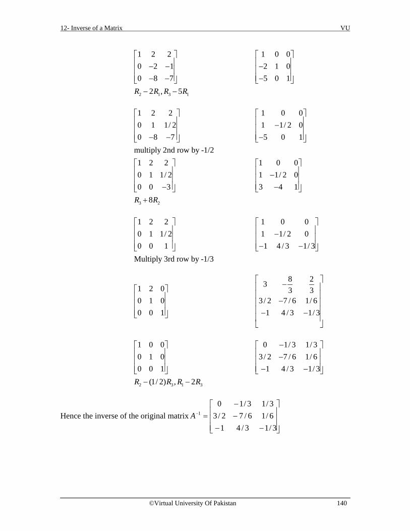
12- Inverse of a Matrix VU
©Virtual University Of Pakistan 140
2 1 3 1
1 2 2 1 0 00 2 1 2 1 00 8 7 5 0 1
2 , 5R R R R
− − − − − −
− −
3 2
1 2 2 1 0 00 1 1/ 2 1 1/ 2 00 8 7 5 0 1
multiply 2nd row by -1/21 2 2 1 0 00 1 1/ 2 1 1/ 2 00 0 3 3 4 1
8R R
− − − −
− − −
+
1 2 2 1 0 00 1 1/ 2 1 1/ 2 00 0 1 1 4 / 3 1/ 3
Multiply 3rd row by -1/3
− − −
8 231 2 0 3 3
0 1 0 3/ 2 7 / 6 1/ 60 0 1 1 4 / 3 1/ 3
− − − −
2 3 1 3
1 0 0 0 1/ 3 1/ 30 1 0 3/ 2 7 / 6 1/ 60 0 1 1 4 / 3 1/ 3
(1/ 2) , 2R R R R
− − − −
− −
Hence the inverse of the original matrix
−−−−
=−
3/13/416/16/72/33/13/10
1A

12- Inverse of a Matrix VU
©Virtual University Of Pakistan 141
Exercises In exercises 1 to 4, find the inverses of the matrices, if they exist. Use elementary row operations.
1. 1 25 9
2. 1 0 51 1 03 2 6
3. 1 4 32 7 6
1 7 2
− − − −
4. 1 3 10 1 21 0 8
− −
5. 3 4 11 0 32 5 4
− −
6. 1 3 4
2 4 14 2 9
− − − −
7. Let 1 5 7
2 5 61 3 4
A− − −
=
. Find the third column of A-1 without computing the other
columns.
8. Let 25 9 27
546 180 537154 50 149
A− − −
=
. Find the second and third columns of A-1 without
computing the first column. 9. Find an elementary matrix E that satisfies the equation. (a) EA = B (b) EB = A (c) EA = C (d) EC = A
where 3 4 1 8 1 5 3 4 12 7 1 , 2 7 1 , 2 7 18 1 5 3 4 1 2 7 3
A B C = − − = − − = − − −
.
10. Consider the matrix 1 0 20 1 00 0 2
A−
=
.
(a) Find elementary matrices E1 and E2 such that E2E1A=I. (b) Write A-1 as a product of two elementary matrices.

12- Inverse of a Matrix VU
©Virtual University Of Pakistan 142
(c) Write A as a product of two elementary matrices. In exercises 11 and 12, express A and A-1 as products of elementary matrices.
11. 2 1 11 2 11 1 2
A =
12. 1 1 01 1 10 1 1
A =
13. Factor the matrix 0 1 7 81 3 3 82 5 1 8
A = − − −
as A = EFGR, where E, F, and G are
elementary matrices and R is in row echelon form.

13- Characterization of Invertible Matrices VU
©Virtual University Of Pakistan 143
Lecture 13
Characterizations of Invertible Matrices
This chapter involves a few techniques of solving the system of n linear equations in n
unknowns and transformation associated with a matrix.
Solving Linear Systems by Matrix Inversion
Theorem
Let A be an n n× invertible matrix. For any b∈Rn , the equation Ax = b …..(1) has the
unique solution i.e. x = A-1b.
Proof
Since A is invertible and b∈ Rn be any vector. Then, we must have a matrix 1A b− which
is a solution of eq. (1) .i.e. Ax = A (A –1b) = Ib = b.
Uniqueness
For uniqueness, we assume that there is another solution u. Indeed, it is a solution of
eq.(1) so it must be u = A-1b, it means x = A-1b = u. This shows that u = x.
Theorem
Let A and B be the square matrices such that AB = I. Then, A and B are invertible with
B = A-1 and A = B-1
Example 1
Solve the system of linear equations
Solution
Consider the linear system
1 2 3
1 2 3
1 3
2 15 3 3
4 6
x x xx x x
x x
+ + =+ + =
+ =
The Matrix form of system is Ax = b, where
1 2 3
1 2 3
1 3
2 15 3 3
4 6
x x xx x x
x x
+ + =+ + =
+ =

13- Characterization of Invertible Matrices VU
©Virtual University Of Pakistan 144
1
2
3
2 1 1 15 1 3 , , 31 0 4 6
xA x x b
x
= = =
Here, det (A) = 2(4) – 1 (20 – 3) + 1(0 – 1) = 8 – 17 – 1 = -10 ≠ 0
So, A is invertible. Now, we apply the inversion algorithm:
2 1 1 1 0 05 1 3 0 1 01 0 4 0 0 1
1 0 4 0 0 15 1 3 0 1 02 1 1 1 0 0
1 2 1 3
1 0 4 0 0 10 1 17 0 1 5 , 5 , 20 1 7 1 0 2
R R R R − − − + − + − −
2 3
1 0 4 0 0 10 1 17 0 1 5 , ,0 0 10 1 1 3
R R − − − + −
3
1 0 4 0 0 10 1 17 0 1 5 ,
101 1 30 0 1
10 10 10
R
− − −
3 1 3 2
2 2 11 0 05 5 5
17 7 10 1 0 , 4 , 1710 10 101 1 30 0 1
10 10 10
R R R R
− −
− − + − + −

13- Characterization of Invertible Matrices VU
©Virtual University Of Pakistan 145
Hence, 1
2 2 15 5 5
17 7 110 10 101 1 3
10 10 10
A−
− −
− = −
Thus, the solution of the linear system is 1 1
2 2 1 25 5 5 51
17 7 1 1310 10 10 5
61 1 3 810 10 10 5
x A b A− −
− − −
− = = = =
−
Example # 2 Solve the system1 2 3
1 2 3
1 3
2 3 52 5 3 3
8 17
x x xx x x
x x
+ + =
+ + = + =
by inversion method.
Solution Consider the linear system1 2 3
1 2 3
1 3
2 3 52 5 3 3
8 17
x x xx x x
x x
+ + =
+ + = + =
This system can be written in matrix form as Ax = b, where
1
2
3
1 2 3 52 5 3 , , 31 0 8 17
xA x x b
x
= = =
Here, [det (A)] = 40 – 2 (16 – 3) + 3(0 – 5) = 40 – 26 – 15 = -1 ≠ 0 Therefore, A is invertible. Now, we apply the inversion algorithm:
1 2 3 1 0 02 5 3 0 1 01 0 8 0 0 1
1 2 3 1 0 00 1 3 2 1 00 2 5 1 0 1
− − − −
1 2 1 32 , 1R R R R− + − +

13- Characterization of Invertible Matrices VU
©Virtual University Of Pakistan 146
1 2 3 1 0 00 1 3 2 1 00 0 1 5 2 1
− − − −
2 32R R+
1 2 3 1 0 00 1 3 2 1 00 0 1 5 2 1
− − − −
31R−
1 2 0 14 6 30 1 0 13 5 30 0 1 5 2 1
− − − − −
3 2 3 13 , 3R R R R+ − +
1 0 0 40 16 90 1 0 13 5 30 0 1 5 2 1
− − − − −
2 12R R− +
Hence, 1
40 16 913 5 35 2 1
A−
− = − − − −
Thus, the solution of the linear system is 1
40 16 9 5 113 5 3 3 15 2 1 17 2
x A b−
− = = − − = − − −
Thus 1 2 31, 1, 2x x x= = − = . Note: It is only applicable when the number of equations = number of unknown and fails
if given matrix is not invertible.
Example 3
Solve the system of linear equation
Solution
The matrix coefficient
1 6 42 4 11 2 5
A = − −
det (A) = 1(20 + 2) – 6(10 – 1) + 4 (4+4)
1 2 3
1 2 3
1 2 3
6 4 22 4 3
2 5 3
x x xx x xx x x
+ + =+ − =
− + + =

13- Characterization of Invertible Matrices VU
©Virtual University Of Pakistan 147
= 22 – 54 + 32
= 0
Thus, A is not invertible. Hence, the inversion method fails.
Solution for the system of a n n× Homogeneous linear equations with
an Invertible Coefficient Matrix:-
Let see if the system is considered as homogeneous then what does the above theorem
say?
Theorem:-
Let Ax = 0 be a homogeneous linear system of n equations and n unknowns. Then, the
coefficient matrix A is invertible iff this system has only a trivial solution.
Example 4
State whether the following system of linear equation has a solution or not?
Solution
We see
2 1 31 3 11 0 4
A = − −
is an invertible matrix (det (A) ≠ 0 )
Thus, this homogeneous linear system has only the trivial solution.
Example 5
Solve1 2 3
2 3
1 2 3
8
2 3 245 5 8
x x xx x
x x x
+ + =
+ = + + =
Solution This system can be written in matrix form as Ax = b, where
1
2
3
1 1 1 80 2 3 , , 245 5 1 8
xA x x b
x
= = =
1 2 3
1 2 3
1 3
2 3 03 0
4 0
x x xx x xx x
+ + =− + =
− =

13- Characterization of Invertible Matrices VU
©Virtual University Of Pakistan 148
Here [det (A)] = 1(2 – 15) – 1(0 – 15) + 1(0 – 10) = -13 + 15 – 10 = -8 ≠ 0 Therefore, A is invertible. Now, we apply the inversion algorithm: A I3
1 1 1 1 0 00 2 3 0 1 05 5 1 0 0 1
1 1 1 1 0 00 2 3 0 1 00 0 4 5 0 1
− −
1 35R R− +
1 1 1 1 0 03 10 1 0 02 2
0 0 4 5 0 1
− −
212
R
1 11 0 1 02 2
3 10 1 0 02 2
0 0 4 5 0 1
− − − −
2 11R R− +
1 11 0 1 02 2
3 10 1 0 02 2
5 10 0 1 04 4
− − −
314
R−
1 11 0 1 02 2
15 1 30 1 08 2 8
5 10 0 1 04 4
− − − −
3 232
R R− +
13 1 11 0 08 2 815 1 30 1 08 2 8
5 10 0 1 04 4
− − − −
3 112
R R+

13- Characterization of Invertible Matrices VU
©Virtual University Of Pakistan 149
Hence, 1
13 1 18 2 815 1 38 2 8
5 104 4
A−
− − = − −
Thus, the solution of the linear system is
1
13 1 18 2 8 8 015 1 3 24 08 2 8
8 85 104 4
x A b−
− − = = − =
−
Thus 1 2 30, 0, 8x x x= = = . Theorem (Invertible Matrix Theorem) Let A be a square n n× matrix. Then the
following statements are equivalent. (Means if any one holds then all are true).
(a) A is an invertible matrix.
(b) A is row equivalent to the n n× identity matrix.
(c) A has n pivot positions.
(d) The equation Ax = 0 has only the trivial solution.
(e) The columns of A form a linearly independent set.
(f) The linear transformation x Ax→ is one-to-one.
(g) The equation Ax = b has at least one solution for each b in Rn.
(h) The columns of A span Rn.
(i) The linear transformation x Ax→ maps Rn onto Rn.
(j) There is a n n× matrix C such that CA = I.
(k) There is a n n× matrix D such that AD = I.
(l) AT is an invertible matrix.
Example 6
Show that the matrix 1 0 41 1 50 1 2
A−
=
is invertible by using Invertible Matrix Theorem

13- Characterization of Invertible Matrices VU
©Virtual University Of Pakistan 150
Solution
By row equivalent,
1 2
2 3
1 0 41 1 5 ,0 1 2
1 0 40 1 9 ,0 1 2
1 0 40 1 90 0 7
A R R
R R
− = − +
− − +
− −
It shows that A has three pivot positions and hence is invertible, by the Invertible Matrix
Theorem (c).
Example 7 Use the Invertible Matrix Theorem to decide if A is invertible, where
1 0 23 1 25 1 9
A−
= − − −
Solution
1 0 2 1 0 20 1 4 0 1 40 1 1 0 0 3
A− −
= − −
Here, A has three pivot positions and hence is
invertible by the Invertible Matrix Theorem (c).
Example 7 Find At and show that At is an invertible matrix.
Solution
1 2 1 02 4 1 11 0 1 10 1 1 1
A
=
1 2 1 02 4 0 11 1 1 10 1 1 1
tA
=

13- Characterization of Invertible Matrices VU
©Virtual University Of Pakistan 151
Now, by row equivalent of A,
2 1 3 1 232 ,1 2 1 0 1 2 1 0 1 2 1 02 4 1 1 0 0 1 1 0 2 0 11 0 1 1 0 2 0 1 0 0 1 10 1 1 1 0 1 1 1 0 1 1 1
R R R R R
A
− −
− − = − −
2 4 21 ( 1) 3 3 42
1 2 1 0 1 2 1 0 1 2 1 01 2 1 01 1 11 0 1 0 0 1 0 0 1 00 1 0 2 2 22
0 0 1 1 0 0 1 1 0 0 1 10 0 1 13 3 50 1 1 1 0 0 1 0 0 1 0 0 02 2 2
R R R R R R− − − − +
− − − − − − − −
Here A has 4 pivot positions so by Invertible Matrix Theorem (c) A is invertible. Thus,
by (l) At is invertible.
Example 8 Use the Invertible Matrix Theorem to decide if A is invertible, where
=
2110210121420121
A
Solution
2 1 3 1 232 ,1 2 1 0 1 2 1 0 1 2 1 02 4 1 2 0 0 1 2 0 2 0 21 0 1 2 0 2 0 2 0 0 1 20 1 1 2 0 1 1 2 0 1 1 2
R R R R R
A
− −
− − = − −

13- Characterization of Invertible Matrices VU
©Virtual University Of Pakistan 152
2 4 21 ( 1) 3 3 42
1 2 1 0 1 2 1 0 1 2 1 0 1 2 1 00 1 0 1 0 1 0 1 0 1 0 1 0 1 0 10 0 1 2 0 0 1 2 0 0 1 2 0 0 1 20 1 1 2 0 0 1 3 0 0 1 3 0 0 0 5
R R R R R R− − − − +
− − − − − − − −
Here, A has 4 pivot positions and hence is invertible by Invertible Matrix Theorem (c).
Solving Multiple Linear Systems with a Common Coefficient Matrix
This technique is used in solving a sequence of linear systems
1 1 2 2, , , k kAx b Ax b Ax b= = = (1)
where coefficient matrix A remains same and off course if it is invertible, then we have a
sequence of solutions. i.e.
1 1 11 1 2 2, , , k kx A b x A b x A b− − −= = = .
Find a Matrix from Linear Transformation
We can find a matrix corresponding to every transformation. In this section we will learn
how to find a matrix attached with a linear transformation.
Example 9
Let L be the linear transformation from R2 to P2 (Polynomials of order 2) defined by
T(x, y) = x y t + (x + y)t2
Find the matrix representing T with respect to the standard bases.
Solution
Let A = {(1,0),(0,1)} be the basis of R2, then
T(1,0) = t2 = (0,0,1) (This triple represents the coefficients of polynomial t2)
i.e. 2 20.1 0. 1.t t t= + +
Similarly, T (0, 1) = t2 = (0,0,1). Hence, the matrix is given by
A= 00 0
1
0
1
Now, we will proceed with a more complicated example.

13- Characterization of Invertible Matrices VU
©Virtual University Of Pakistan 153
Example 10
Let T be the linear transformation from R2 to R2 such that T(x, y) = (x , y + 2x). Find a
matrix A for T.
Solution
This matrix is found by finding T (1, 0) = (1, 2) and T (0, 1) = (0, 1)The matrix
is1 02 1
A =
.
Important Note
It should be clear that the Invertible Matrix Theorem applies only to square matrices. For
example, if the columns of a 4 3× matrix are linearly independent, we cannot use the
Invertible Matrix Theorem to conclude any thing about the existence or nonexistence of
solutions to equations of the form Ax = b.
Invertible Linear Transformations
Recall that matrix multiplication corresponds to composition of linear transformations. When a matrix A is invertible, the equation A-1Ax = x can be viewed as a statement about linear transformations. See Figure 2.
Multiplication
by A x• • Ax Multiplication
by A-1
Figure 2 A-1 transforms Ax back to x
Definition
A linear transformation : n nT R R→ be a linear Transformation and A be a standard
matrix for T. Then, T is invertible if and only if A is an invertible matrix in that case
linear transformation S given by S(x) = A-1x is a unique function satisfying (1) and (2)
( ( )) (1)( ( )) (2)
n
n
S T x x x RT S x x x R
= ∀ ∈
= ∀ ∈

13- Characterization of Invertible Matrices VU
©Virtual University Of Pakistan 154
Important Note
If the inverse of a linear transformation exits then it is unique.
Proposition
Let : n mT R R→ be linear transformation, given as ( ) , nT x Ax x R= ∀ ∈ , where A is
a m n× matrix. The mapping T is invertible if the system y Ax= has a unique solution.
Case 1:
If m n< , then the system Ax y= has either no solution or infinitely many solutions, for
any y in Rm. Therefore, y Ax= is non-invertible.
Case 2:
If m n= , then the system Ax y= has a unique solution if and only if Rank (A) = n.
Case 3:
If m n> , then the transformation y Ax= is non-invertible because we can find a vector
y in Rm such that Ax y= is inconsistent.

13- Characterization of Invertible Matrices VU
©Virtual University Of Pakistan 155
Exercises
1.Solve the system of linear equations by inverse matrix method.
2. Let 1 2 3 4
1 2 5 2 3 1, , , ,
3 8 7 2 5 7A b b b and b
− = = = = = −
.
(a) Find A-1 and use it to solve the equations Ax = b1, Ax = b2, Ax = b3, Ax = b4.
(b) Solve the four equations in part (a) by row reducing the augmented matrix
[ ]1 2 3 4A b b b b .
3. (a) Solve the two systems of linear equations
1 2 3
1 2 3
2 3
2 13 2 3
2 4
x x xx x x
x x
+ + = −+ + =
+ =
&
1 2 3
1 2 3
2 3
2 03 2 0
2 4
x x xx x x
x x
+ + =+ + =
+ =
by row reduction.
(b) Write the systems in (a) as Ax = b1 and Ax = b2, and then solve each of them by the
method of inversion.
Determine which of the matrices in exercises 4 to 10 are invertible?
4. 4 16
3 9−
− 5.
5 0 37 0 29 0 1
6. 2 3 42 3 42 3 4
7. 5 9 30 3 41 0 3
−
1 2 3
2 3
1 2 3
4 2
2 3 45 3
x x xx x
x x x
+ + =
+ =+ − =

13- Characterization of Invertible Matrices VU
©Virtual University Of Pakistan 156
8.
1 3 0 10 1 2 12 6 3 2
3 5 8 3
− − − − − −
9.
1 0 0 02 5 0 03 6 8 04 7 9 10
10.
7 6 4 15 1 0 2
10 11 7 319 9 7 1
− − − − −
11.
5 4 3 6 37 6 5 9 58 6 4 10 49 8 9 5 8
10 8 7 9 7
− − −
12. Suppose that A and B are n n× matrices and the equation ABx = 0 has a nontrivial
solution. What can you say about the matrix AB?
13. What can we say about a one-to-one linear transformation T from Rn into Rn?
14. Let 2 2:T R R→ be a linear transformation given as ( ) 5T x x= , then find a matrix A of
linear transformation T.
In exercises 15 and 16, T is a linear transformation from R2 into R2. Show that T is
invertible.
15. 1 2 1 2 1 2( , ) ( 5 9 ,4 7 )T x x x x x x= − + −
16. 1 2 1 2 1 2( , ) (6 8 , 5 7 )T x x x x x x= − − +
17. Let : n nT R R→ be a linear transformation and let A be the standard matrix for T.
Then T is invertible if and only if A is an invertible matrix.

14-Partitioned Matrices VU
©Virtual University Of Pakistan 157
Lecture 14
Partitioned Matrices A block matrix or a partitioned matrix is a partition of a matrix into rectangular
smaller matrices called blocks.Partitioned matrices appear often in modern applications
of linear algebra because the notation simplifies many discussions and highlights
essential structure in matrix calculations. This section provides an opportunity to review
matrix algebra and use of the Invertible Matrix Theorem.
General Partitioning of a Matrix - A matrix can be partitioned (subdivided) into sub matrices (also called blocks) in
various ways by inserting lines between selected rows and columns.
Example 1
The matrix
1 1 2 21 1 2 23 3 4 43 3 4 4
P
=
can be partitioned into four 2×2 blocks
11 12 21 22
1 1 2 2 3 3 4 4, , , ,
1 1 2 2 3 3 4 4P P P P
= = = =
The partitioned matrix can then be written as
Example 2
The matrix3 0 1 5 9 2
5 2 4 0 3 1
8 6 3 1 7 4
A − −
= − − − − −
can also be written as the 2 3× partitioned (or block) matrix
11 12
21 22
P PP
P P
=
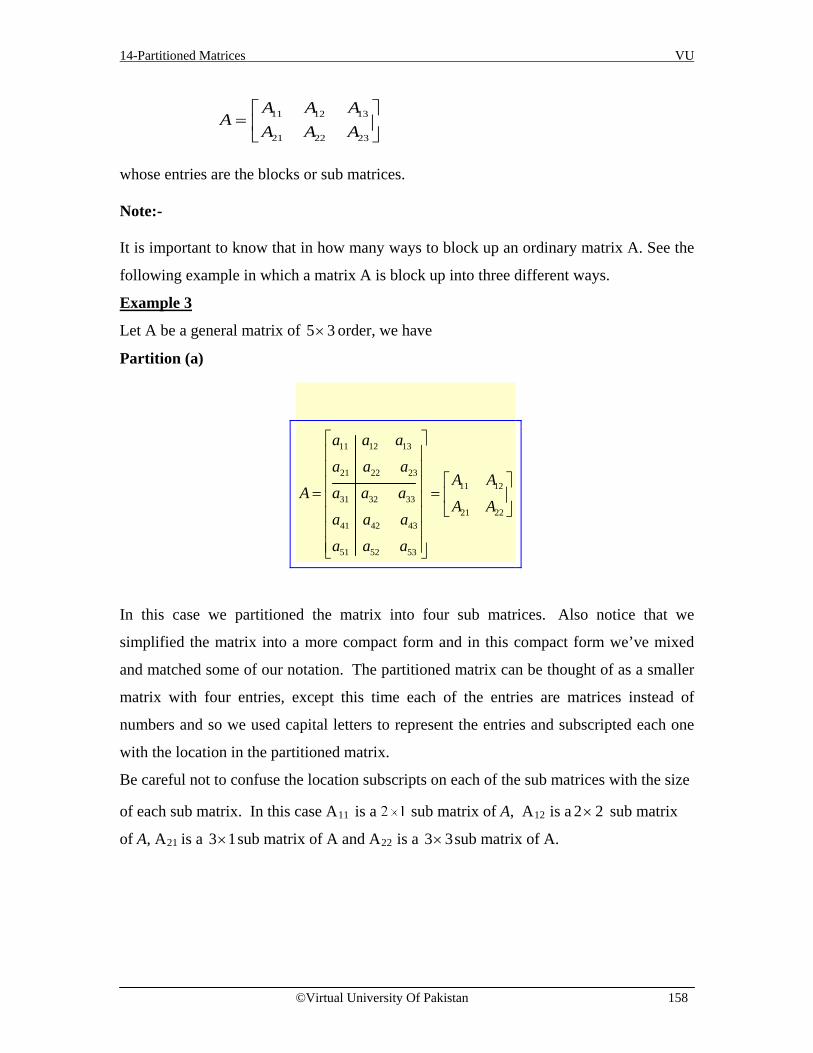
14-Partitioned Matrices VU
©Virtual University Of Pakistan 158
whose entries are the blocks or sub matrices. Note:- It is important to know that in how many ways to block up an ordinary matrix A. See the
following example in which a matrix A is block up into three different ways.
Example 3
Let A be a general matrix of 5 3× order, we have
Partition (a)
11 12 13
21 22 2311 12
31 32 3321 22
41 42 43
51 52 53
a a a
a a aA A
A a a aA A
a a a
a a a
= =
In this case we partitioned the matrix into four sub matrices. Also notice that we
simplified the matrix into a more compact form and in this compact form we’ve mixed
and matched some of our notation. The partitioned matrix can be thought of as a smaller
matrix with four entries, except this time each of the entries are matrices instead of
numbers and so we used capital letters to represent the entries and subscripted each one
with the location in the partitioned matrix.
Be careful not to confuse the location subscripts on each of the sub matrices with the size
of each sub matrix. In this case A11 is a sub matrix of A, A12 is a 2 2× sub matrix
of A, A21 is a 3 1× sub matrix of A and A22 is a 3 3× sub matrix of A.
11 12 13
21 22 23
A A AA
A A A
=

14-Partitioned Matrices VU
©Virtual University Of Pakistan 159
Partition (b)
[ ]
11 12 13
21 22 23
31 32 33 1 2 3
41 42 43
51 52 53
a a a
a a a
A a a a c c c
a a a
a a a
= =
In this case, we partitioned A into three column matrices each representing one column in
the original matrix. Again, note that we used the standard column matrix notation (the
bold face letters) and subscripted each one with the location in the partitioned matrix.
The ci in the partitioned matrix are sometimes called the column matrices of A.
Partition (c)
11 12 13 1
21 22 23 2
31 32 33 3
441 42 43
551 52 53
a a a ra a a r
A a a a rra a ara a a
= =
Just as we can partition a matrix into each of its columns as we did in the previous part
we can also partition a matrix into each of its rows. The ri in the partitioned matrix are
sometimes called the row matrices of A.
Addition of Blocked Matrices
If matrices A and B are the same size and are partitioned in exactly the same way, then it
is natural to make the same partition of the ordinary matrix sum A + B. In this case, each
block of A + B is the (matrix) sum of the corresponding blocks of A and B.
Theorem If A is m×n and B is n×p, then

14-Partitioned Matrices VU
©Virtual University Of Pakistan 160
AB = 1 2( ) ( ) ... ( )nCol A Col A Col A+ + +
1
2
( )( )
( )n
Row BRow B
Row B
Proof For each row index I and column index j, the (i,j) entry in colk (A) rowk (B) is the product
of aik from colk (A) and bkj from rowk (B).
Hence, the (i,j)-entry in the sum shown in (2) is
1 1 21 2 1...
( 1, 2,..., )i j j n nja b a b a bk n
+ + +
=
This sum is also the (i,j)- entry in AB by the row column rule
Example 4 Let
11 12 11 12
21 22 21 22
A A B BA and B
A A B B
= =
, then
11 12 11 12
21 22 21 22
11 11 12 12
21 21 22 22
A A B BA B
A A B B
A B A BA B A B
+ = +
+ + = + +
Similarly, subtraction of blocked matrices is defined.
Multiplication of a partitioned matrix by a scalar is also computed block by block.
Multiplication of Partitioned Matrices
If 11 12
11 1221 22
21 2231 32
A AB B
A A A and BB B
A A
= =
and if the sizes of the blocks confirm for the required operations, then
1 1 2 2( ) ( ) ( ) ( ) ... ( ) ( )n nCol A Row B Col A Row B Col A Row B= + + +
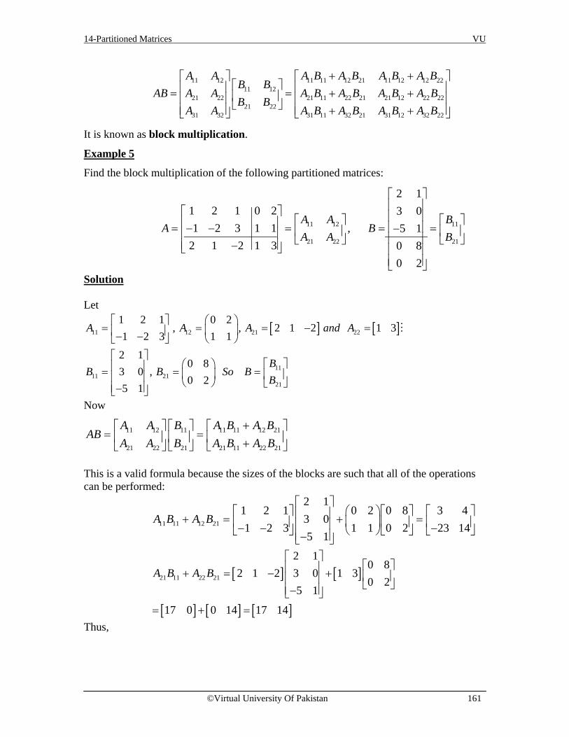
14-Partitioned Matrices VU
©Virtual University Of Pakistan 161
11 12 11 11 12 21 11 12 12 22
11 1221 22 21 11 22 21 21 12 22 22
21 2231 32 31 11 32 21 31 12 32 22
A A A B A B A B A BB B
AB A A A B A B A B A BB B
A A A B A B A B A B
+ + = = + + + +
It is known as block multiplication.
Example 5
Find the block multiplication of the following partitioned matrices:
11 12 11
21 22 21
2 11 2 1 0 2 3 01 2 3 1 1 , 5 1
2 1 2 1 3 0 80 2
A A BA B
A A B
= − − = = =− −
Solution Let
[ ] [ ]11 12 21 22
1111 21
21
1 2 1 0 2, , 2 1 2 1 3
1 2 3 1 1
2 10 8
3 0 ,0 2
5 1
A A A and A
BB B So B
B
= = = − = − −
= = = −
Now
This is a valid formula because the sizes of the blocks are such that all of the operations can be performed:
11 11 12 21
2 11 2 1 0 2 0 8 3 4
3 01 2 3 1 1 0 2 23 14
5 1A B A B
+ = + = − − − −
[ ] [ ]
[ ] [ ] [ ]
21 11 22 21
2 10 8
2 1 2 3 0 1 30 2
5 1
17 0 0 14 17 14
A B A B
+ = − + − = + =
Thus,
11 12 11 11 11 12 21
21 22 21 21 11 22 21
A A B A B A BAB
A A B A B A B+
= = +

14-Partitioned Matrices VU
©Virtual University Of Pakistan 162
11 11 12 21
21 11 22 21
3 623 12
17 14
A B A BAB
A B A B
+ = = − +
Note - We see result is same when we multiply A and B without partitions
2 11 2 1 0 2 3 63 01 2 3 1 1 23 125 1
2 1 2 1 3 17 140 80 2
AB
= − − = −− −
Note - Sometimes it is more useful to find the square and cube powers of a matrix.
Example 6 The block version of the row –column rule for the product AB of the partitioned matrices
11 12 11
21 22 21
11 21
2 13 4 1 0 2 3 01 5 3 1 4 , 5 1
2 0 2 1 6 4 30 2
2 14 3
3 00 2
5 1
A A BA B
A A B
where
B and B
− − = − − = = =− − −
− − = = −
So
11 12 11 11 11 12 21
21 22 21 21 11 22 21
A A B A B A BAB
A A B A B A B+
= = +
This is a valid formula because the sizes of the blocks are such that all of the operations can be performed:
11 11 12 21
2 13 4 1 0 2 4 3 11 2
3 01 5 3 1 4 0 2 32 3
5 1A B A B
− − − − + = + = − − −
[ ] [ ] [ ]21 11 22 21
2 14 3
2 0 2 3 0 1 6 18 50 2
5 1A B A B
− − + = − + = −
Thus,

14-Partitioned Matrices VU
©Virtual University Of Pakistan 163
11 11 12 21
21 11 22 21
11 232 318 5
A B A BAB
A B A B
− + = = +
This result can be confirmed by performing the computation.
2 13 4 1 0 2 11 23 01 5 3 1 4 32 35 1
2 0 2 1 6 18 54 30 2
AB
− − − = − − =− − −
Example 7 Making block up of matrix
2 0 0 0 20 2 0 0 20 0 2 0 20 0 0 2 00 0 0 0 2
A
=
, evaluate 2A ?
Solution We partition A as shown below
2 0 0 0 20 2 0 0 20 0 2 0 20 0 0 2 00 0 0 0 2
A
=
where 32
0 20 2 ,0 2
A =
Now
3 32 3 322
23 2 23 2
3 32
23 2
2 22 2
4 44
I A I AA
O I O I
I AO I
=
=

14-Partitioned Matrices VU
©Virtual University Of Pakistan 164
Hence
2
4 0 0 0 80 4 0 0 80 0 4 0 80 0 0 4 00 0 0 0 4
A
=
Example 8
Let
1 0 0 0 0 10 1 0 0 0 10 0 1 0 0 10 0 0 1 0 00 0 0 0 1 01 1 1 0 0 1
A
=
Evaluate 2A ?
Solution We partition A as shown below
3 32 1
23 2 21
1 12
1 0 0 0 0 10 1 0 0 0 10 0 1 0 0 10 0 0 1 0 0
10 0 0 0 1 01 1 1 0 0 1
t
I O AA O I O
A O
= =
where 1
111
A =
Now 3 32 1 3 32 1 3 1 1 32 1 1
223 2 21 23 2 21 23 2 21
1 12 1 12 1 1 12 1 11 1 1
t
t t t t t
I O A I O A I A A O A AA O I O O I O O I O
A O A O A A O A A
+ + = = + +
[ ]
[ ]
3 1 1 1 1 1 1
1 1
2 1 1 21 2 1 , 2 , 2 2 21 1 2 2
1 4
t t t
t
I A A A A A A
A A
+ = + = + =
+ =

14-Partitioned Matrices VU
©Virtual University Of Pakistan 165
Hence 2
2 1 1 0 0 21 2 1 0 0 21 1 2 0 0 20 0 0 1 0 00 0 0 0 1 02 2 2 0 0 4
A
=
Toeplitz matrix
A matrix in which each descending diagonal from left to right is constant is called a Toeplitz matrix or diagonal-constant matrix
Example 9 The matrix
1 2 34 1 25 4 16 5 4
aa
Aa
a
=
is a Toeplitz matrix.
Block Toeplitz matrix
A blocked matrix in which blocks (blocked matrices) are repeated down the diagonals of the matrix is called a blocked Toeplitz matrix.
A block Toeplitz matrix B has the form
B =
(1,1) (1,2) (1,3) (1,4) (1,5)(2,1) (1,1) (1,2) (1,3) (1,4)(3,1) (2,1) (1,1) (1,2) (1,3)(4,1) (3,1) (2,1) (1,1) (1,2)(5,1) (4,1) (3,1) (2,1) (1,1)
B B B B BB B B B BB B B B BB B B B BB B B B B
Inverses of Partitioned Matrices
In this section, we will study about the techniques of inverse of blocked matrices. Block Diagonal Matrices
A partitioned matrix A is said to be block diagonal if the matrices on the main diagonal
are square and all other position matrices are zero, i.e.

14-Partitioned Matrices VU
©Virtual University Of Pakistan 166
1
2
0 ... 00 ... 0
0 0 ... k
DD
A
D
=
(1)
where the matrices D1, D2, …, Dk are square. It can be shown that the matrix A in (1) is
invertible if and only if each matrix on the diagonal is invertible. i.e.
11
11 2
1
0 ... 00 ... 0
0 0 ... k
DD
A
D
−
−−
−
=
Example 10 Let A be a block diagonal matrix
1 2 0 0 01 1 0 0 00 0 1 1 00 0 5 4 00 0 0 0 2
A
− =
Find −1A .
Solution
There are three matrices on the main diagonal; two are 2x2 matrices and one
is1 1× matrix.
In order to find −1A , we evaluate the inverses of three matrices lie in main diagonal of A.
Let ( )11 22 33
1 2 1 1, 2
1 1 5 4A A and A
= = = − are matrices of main diagonal of A. Then
1 1111
11
1 2 1 21 1 3 3
1 133 3
AdjAA
A−
− − − = = =
−−
.

14-Partitioned Matrices VU
©Virtual University Of Pakistan 167
Similarly 1
22
122
4 15 1
14 1
5 1
A
A
−
−
− − =
−−
= −
−
−
⇒ = − −
A 1
1 2 0 0 03 31 1 0 0 03 30 0 4 1 00 0 5 1 0
10 0 0 02
Example 11 Consider the block diagonal matrix
8 7 0 0 01 1 0 0 00 0 3 1 00 0 5 2 00 0 0 0 4
A
− − =
There are three matrices on the main diagonal – two 2x2 matrices and one 1x1 matrix.
−
− − −⇒ = −
A 1
1 7 0 0 01 8 0 0 00 0 2 1 00 0 5 3 0
10 0 0 04
Block Upper Triangular Matrices
A partitioned square matrix A is said to be block upper triangular if the matrices on the
main diagonal are square and all matrices below the main diagonal are zero; that is, the
matrix is partitioned as

14-Partitioned Matrices VU
©Virtual University Of Pakistan 168
=
k
k
kk
A A AO A A
A
O O A
11 12 1
22 2
...
...
...
where the matrices A11, A22,…, Akk are
square.
Note The definition of block lower triangular matrix is similar.
Here, we are going to introduce a formula for finding inverse of a block upper triangular
matrix in the following example.
Example 12
Let A be a block upper triangular matrix of the form
11 12
220A A
AA
=
where the orders of A11 and A22 are p p× and q q× respectively. Find A-
1.
Solution
Let B = 11 12
21 22
B BB B
be inverse of A .i.e. A-1 = B, then
11 12 11 12
22 21 22
11 11 12 21 11 12 12 22
22 21 22 22
p
q
p
q
I OA A B BAB
O IO A B B
I OA B A B A B A BO IA B A B
= =
+ + =
By comparing corresponding entries, we have
11 11 12 21A B A B+ = pI (1)
11 12 12 22A B A B+ = O (2)
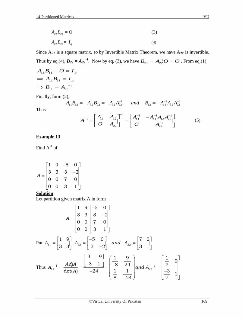
14-Partitioned Matrices VU
©Virtual University Of Pakistan 169
22 21A B = O (3)
22 22A B = qI (4)
Since A22 is a square matrix, so by Invertible Matrix Theorem, we have A22 is invertible.
Thus by eq.(4), B22 = A22-1. Now by eq. (3), we have 1
21 22B A O O−= = . From eq.(1)
11 11
11 11
111 11
p
p
A B O IA B I
B A −
+ =
⇒ =
⇒ =
Finally, form (2), 1 1 1
11 12 12 22 12 22 12 11 12 22A B A B A A and B A A A− − −= − = − = − Thus
1 1 1 1
11 121 11 11 12 221
22 22
A A A A A AA
O A O A
− − − −−
−
− = =
(5)
Example 13 Find A-1 of
Solution Let partition given matrix A in form
− − =
1 9 5 03 3 3 20 0 7 00 0 3 1
A
Put −
= = = − 11 12 22
1 9 5 0 7 0,
3 3 3 2 3 1A A and A
Thus − −
− − − = = = =
−− −
1 111 22
3 9 1 9 1 03 1 8 24 71 1 3det( ) 24 18 24 7
AdjAA and AA
− − =
1 9 5 03 3 3 20 0 7 00 0 3 1
A

14-Partitioned Matrices VU
©Virtual University Of Pakistan 170
Moreover,
- − −
− − −= = −− − −
1 111 12 22
1 9 4 31 05 08 24 7 471 11 1 3 2 3 14 128 24 7
A A A
So by (5), we have
Example 14
Confirm that
− − =
A
4 7 5 33 5 3 20 0 7 20 0 3 1
is an invertible block upper triangular matrix, and
then find its inverse by using formula (9). Solution The matrix is block upper triangular because it can be partitioned into form
=
k
k
kk
A A AO A A
A
O O A
11 12 1
22 2
...
...
...
as
− − = =
A AA
O A11 12
22
4 7 5 33 5 3 20 0 7 20 0 3 1
where −
= = = − A A A11 12 22
4 7 5 3 7 2, ,
3 5 3 2 3 1
Now − −− − = = − −
A and A1 111 22
5 7 1 23 4 3 7
−
− −
− − =
−
1
1 3 4 38 8 7 4
11 1 1
128 24 4
10 0 0730 0 17
A

14-Partitioned Matrices VU
©Virtual University Of Pakistan 171
Moreover, − − − − − − − = − = − − − − A A A1 1
11 12 22
5 7 5 3 1 2 133 2953 4 3 2 3 7 78 173
So it follows from (9) that the inverse of A is −
− − − − = − −
A 1
5 7 133 2953 4 78 1730 0 1 20 0 3 7
NUMERICAL NOTES
1. When matrices are too large to fit in a computer’s high-speed memory, partitioning permits a computer to work with only two or three sub-matrices at a time. For instance, in recent work on linear programming, a research team simplified a problem by partitioning the matrix into 837 rows and 51 columns. The problem’s solution took about 4 minutes on a Cray supercomputer.
2. Some high-speed computers, particularly those with vector pipeline
architecture, perform matrix calculations more efficiently when the algorithms use partitioned matrices.
3. The latest professional software for high-performance numerical linear
algebra, LAPACK, makes intensive use of partitioned matrix calculations. The exercises that follow give practice with matrix algebra and illustrate typical calculations found in applications.

14-Partitioned Matrices VU
©Virtual University Of Pakistan 172
Exercises In exercises 1 to 3, the matrices A, B, C, X, Y, Z, and I are all n x n and satisfy the indicated equation.
1. 0 0
0 0A B I IC X Y Z
=
2. 0 0 0
0X A IY Z B C I
=
3. 0 0 0
0 00 0
A ZX IY I I
B I
=
4. Suppose that A11 is an invertible matrix. Find matrices X and Y such that the product below has the form indicated. Also compute B22.
11 12 11 12
21 22 22
31 32 32
0 00 0
0 0
I A A B BX I A A BY I A A B
=
5. The inverse of 0 0 0 0
0 0I IC I is Z IA B I X Y I
. Find X, Y and Z.
6. Find the Inverse of matrix A.
8 3 0 0 01 4 0 0 00 0 3 1 00 0 5 1 00 0 0 0 8
A
=
7. Show that 0I
A I
is invertible and find its inverse.
8. Compute XTX, when X is partitioned as [X1 X2]. In exercises 9 and 10, determine whether block multiplication can be used to compute the product using the partitions shown. If so, compute the product by block multiplication.

14-Partitioned Matrices VU
©Virtual University Of Pakistan 173
9. (a)
2 1 41 2 1 5
3 5 20 3 4 2
7 1 51 5 6 1
0 3 3
− − − − − −
(b)
2 1 41 2 1 5
3 5 20 3 4 2
7 1 51 5 6 1
0 3 3
− − − − − −
10. (a)
2 4 13 1 0 3 3 0 22 1 4 5 1 3 5
2 1 4
− − − −
(b)
2 51 3 2 1 3 40 5 0 1 5 71 4
− − −
11. Compute the product 3 1 1 2 02 4 1 6 2 − −
using the column row-rule, and check
your answer by calculating the product directly.
In exercises 11 and 12, find the inverse of the block diagonal matrix A.
12. (a)
2 1 0 03 2 0 00 0 3 40 0 1 1
A
= −
(b)
5 2 0 0 03 1 0 0 00 0 5 0 00 0 0 2 70 0 0 1 4
13. (a)
5 1 0 04 1 0 00 0 2 30 0 3 5
A
= − −
(b)
2 0 0 0 00 1 2 0 00 3 7 0 00 0 0 4 90 0 0 1 2
14. Find the inverse of the block upper triangular matrix A.
(i)
2 1 3 61 1 7 40 0 3 50 0 2 3
A
− =
(ii)
1 1 2 52 1 3 80 0 4 10 0 7 2
A
− − − =
15. Find B1, given that 3 31 1 2 2
31 2 00 0A BA B A B
CC C
=
and

14-Partitioned Matrices VU
©Virtual University Of Pakistan 174
1 2 1
2 2 3
2 0 1 1 1 1, ,
0 1 1 2 1 1
2 0 1 0 2 1, ,
0 2 0 2 1 3
A B C
A C B
= = = −
= = =
16. Consider the partitioned linear system
1
2
3
4
5 2 2 3 22 1 3 1 61 0 4 1 00 1 0 2 0
xxxx
− =
l
Solve this system by first expressing it as
0A B u bI D v
=
or equivalently,
0Au Bv bu Dv
+ =+ =
next solving the second equation for u in terms of v, and then substituting in the first equation. Check your answer by solving the system directly.
17. Let 3 1 2
.1 4 5
a bA and B c d
e f
− = = −
Verify that 1 1 2 2 3 3( ) ( ) ( ) ( ) ( ) ( )AB col A row B col A row B col A row B= + +
18. Find inverse of the matrix
− − =
A
4 7 5 33 5 3 20 0 7 20 0 3 1
.

15- Matrix Factorizations VU
©Virtual University Of Pakistan 175
Lecture 15
Matrix Factorizations
Matrix Factorization A factorization of a matrix as a product of two or more matrices is called Matrix Factorization. Uses of Matrix Factorization Matrix factorizations will appear at a number of key points throughout the course. This lecture focuses on a factorization that lies at the heart of several important computer programs widely used in applications. LU Factorization or LU-decomposition LU factorization is a matrix decomposition which writes a matrix as the product of a lower triangular matrix and an upper triangular matrix. This decomposition is used to solve systems of linear equations or calculate the determinant. Assume A is an m n× matrix that can be row reduced to echelon form, without row interchanges. Then A can be written in the form A = LU, where L is an m m× lower triangular matrix with 1’s on the diagonal and U is an m n× echelon form of A. For instance, such a factorization is called LU factorization of A. The matrix L is invertible and is called a unit lower triangular matrix.
LU factorization.
Remarks 1) If A is the square matrix of order m, then the order of both L and U will also be m. 2) In general, not every square matrix A has an LU-decomposition, nor is an LU-decomposition unique if it exists. Theorem If a square matrix A can be reduced to row echelon form with no row interchanges, then A has an LU-decomposition. Note The computational efficiency of the LU factorization depends on knowing L and U. The next algorithm shows that the row reduction of A to an echelon form U amounts to an LU factorization because it produces L with essentially no extra work. An LU Factorization Algorithm Suppose A can be reduced to an echelon form U without row interchanges. Then, since row scaling is not essential, A can be reduced to U with only row replacements, adding a
1 0 0 0 * * * ** 1 0 0 0 * * ** * 1 0 0 0 0 ** * * 1 0 0 0 0 0
A
L U
• • = •

15- Matrix Factorizations VU
©Virtual University Of Pakistan 176
multiple of one row to another row below it. In this case, there exist lower triangular elementary matrices E1, …, Ep such that
Ep … E1A = U (1) So A = (Ep …E1)-1U = LU Where L = (Ep … E1)-1 (2) It can be shown that products and inverses of unit lower triangular matrices are also unit-lower triangular. Thus, L is unit-lower triangular. Note that the row operations in (1), which reduce A to U, also reduce the L in (2) to I, because Ep … E1L = (Ep…E1)(Ep … E1)-1 = I. This observation is the key to constructing L. Procedure for finding an LU-decomposition Step 1: Reduce matrix A to row echelon form U without using row interchanges, keeping track of the multipliers used to introduce the leading 1’s and the multipliers used to introduce zeros below the leading 1’s. Step 2: In each position along the main diagonal of L, place the reciprocal of the multiplier that introduced the leading 1 in that position in U. Step 3: In each position below the main diagonal of L, place the negative of the multiplier used to introduce the zero in that position in U. Step 4: Form the decomposition A = LU. Example 1 Find an LU-decomposition of
6 -2 0A= 9 -1 1
3 7 5
Solution We will reduce A to a row echelon form U and at each step we will fill in an entry of L in accordance with the four-step procedure above.
6 -2 0
A= 9 -1 13 7 5
* 0 0* * 0* * *
* denotes an unknown entry of L.
13
16
1 - 09 -1 1 multiplier =3 7 5
←
6 0 0* * 0* * *
131 0
90 2 1
30 8 5
multipliermultiplier
− ← = −
← = −
6 0 09 * 03 * *

15- Matrix Factorizations VU
©Virtual University Of Pakistan 177
13
12
1 010 12
0 8 5
multiplier
− ← =
6 0 09 2 03 * *
13
12
1 00 1 8
0 0 1
multiplier −
← = −
6 0 09 2 03 8 *
13
12
1 00 1 1
0 0 1
−
= ← =
U multiplier 6 0 09 2 03 8 1
=
L
(No actual operation is performed here since there is already a leading 1 in the third row.) So
13
12
6 0 0 1 09 2 0 0 13 8 1 0 0 1
A LU−
= =
OR Solution We will reduce A to a row echelon form U and at each step we will fill in an entry of L in accordance with the four-step procedure above.
6 -2 0
A= 9 -1 13 7 5
* 0 0* * 0* * *
* denotes an unknown entry of L.
116
6 -2 06 6 69 -1 1 R3 7 5
≈
6 0 0* * 0* * *
-11 03
9 -1 13 7 5
=

15- Matrix Factorizations VU
©Virtual University Of Pakistan 178
)
)
-11 03
-19 - 9(1) -1- 9( 1- 9(0)3
-13 - 3(1) 7 - 3( 5 - 3(0)3
≈
2 1
3 1
93
R RR R
−−
6 0 09 * 03 * *
-11 03
0 2 10 8 5
=
212
-11 03
0 2 1 R2 2 20 8 5
≈
6 0 09 2 03 * *
-11 03
10 12
0 8 5
=
3 28
)
-11 03
10 1 R R2
10 - 8(0) 8 - 8(1) 5 - 8(2
≈ −
6 0 09 2 03 8 *
-11 03
10 12
0 0 1
=

15- Matrix Factorizations VU
©Virtual University Of Pakistan 179
13
12
1 00 1 1
0 0 1
−
= ← =
U multiplier 6 0 09 2 03 8 1
=
L
So
13
12
6 0 0 1 09 2 0 0 13 8 1 0 0 1
A LU−
= =
Example 2 Find an LU factorization of
2 4 2 36 9 5 82 7 3 94 2 2 16 3 3 4
A
− − − − = − − − − − −
Solution
2 4 2 36 9 5 82 7 3 94 2 2 16 3 3 4
− − − − = − − − − − −
A
1 0 0 0 0* 1 0 0 0* * 1 0 0* * * 1 0* * * * 1
* denotes an unknown entry of L.
3 11 2 12 2
6 9 5 82 7 3 94 2 2 16 3 3 4
− − ←
− − − −
− − − −
multiplier
2 0 0 0 0* 1 0 0 0* * 1 0 0* * * 1 0* * * * 1
31 2 12
60 3 1 120 3 1 640 6 2 7
60 9 3 13
− − ← −−
← − − − ← −−
← − −
multipliermultipliermultipliermultiplier
2 0 0 0 06 1 0 0 02 * 1 0 04 * * 1 0-6 * * * 1

15- Matrix Factorizations VU
©Virtual University Of Pakistan 180
31 2 12
11 10 1 33 30 3 1 60 6 2 70 9 3 13
− −
← − − − −
− −
multiplier
2 0 0 0 06 3 0 0 02 * 1 0 04 * * 1 0-6 * * * 1
31 2 12
1 10 13 3 3
0 0 0 5 60 0 0 5 90 0 0 10
− − − ←
← − − ←
multipliermultipliermultiplier
2 0 0 0 06 3 0 0 02 -3 1 0 04 6 * 1 0-6 -9 * * 1
31 2 12
1 10 1 13 350 0 0 5
0 0 0 10 0 0 10
− − − ← −
multiplier
2 0 0 0 06 3 0 0 02 -3 1 0 04 6 0 -5 0-6 -9 0 * 1
31 2 12
1 10 13 3 10
0 0 0 50 0 0 10 0 0 0
− − − = ← −
U multiplier
2 0 0 0 06 3 0 0 02 -3 1 0 04 6 0 -5 0-6 -9 0 10 1
=
L
Thus, we have constructed the LU-decomposition 31 -2 -12 0 0 0 0 2
1 16 3 0 0 0 0 1 -3 32 -3 1 0 0
0 0 0 54 6 0 -5 00 0 0 1-6 -9 0 10 10 0 0 0
= =
A LU

15- Matrix Factorizations VU
©Virtual University Of Pakistan 181
Example 3 Find LU–decomposition of
6 -2 -4 43 -3 -6 1
A =-12 8 21 -8-6 0 -10 7
Solution
6 2 4 43 3 6 112 8 21 86 0 10 7
A
− − − − = − − − −
1 0 0 0* 1 0 0* * 1 0* * * 1
L
=
* denotes an unknown entry of L.
1 2 2 113 3 3 6
3 3 6 112 8 21 86 0 10 7
multiplier − − ←
− − − − − −
6 0 0 0* 1 0 0* * 1 0* * * 1
1 2 213 3 3
30 2 4 1120 4 13 060 2 14 11
multipliermultipliermultiplier
− − ← −− − −
← ←− −
6 0 0 03 1 0 012 * 1 06 * * 1
− −
1 2 213 3 3
110 1 2 220 4 13 00 2 14 11
multiplier
− −
← − − −
6 0 0 03 2 0 012 * 1 06 * * 1
− − −

15- Matrix Factorizations VU
©Virtual University Of Pakistan 182
1 2 213 3 3
10 1 22 4
0 0 5 2 20 0 10 12
multipliermultiplier
− − ← − − ← −
6 0 0 03 2 0 012 4 1 06 2 * 1
− − − −
1 2 213 3 3
10 1 222 10 0 15 5
0 0 10 12
multiplier
− − − ← −
6 0 0 03 2 0 012 4 5 06 2 * 1
− − − −
1 2 21 - -3 3 3
10 1 2220 0 1 - multiplier 105
0 0 0 8
←
6 0 0 03 2 0 012 4 5 06 2 10 1
− − − − −
1 2 213 3 3
10 1 222 10 0 15 8
0 0 0 1
U
multiplier
− − = − ←
6 0 0 03 2 0 012 4 5 06 2 10 8
L
− = − − − −
1 2 213 3 36 0 0 0
13 2 0 0 0 1 22
12 4 5 0 20 0 16 2 10 8 50 0 0 1
Thus A LU
− − − = = − −− − −

15- Matrix Factorizations VU
©Virtual University Of Pakistan 183
Example 4 Find an LU factorization of
2 4 1 5 24 5 3 8 12 5 4 1 86 0 7 3 1
A
− − − − − = − − − −
Solution
2 4 1 5 24 5 3 8 12 5 4 1 86 0 7 3 1
A
− − − − − = − − − −
1 0 0 0* 1 0 0* * 1 0* * * 1
L
=
* denotes an unknown entry of L.
− − ← − − − − − − −
1 5 11 2 12 2 2
4 5 3 8 12 5 4 1 86 0 7 3 1
multiplier
2 0 0 0* 1 0 0* * 1 0* * * 1
− − ←−
← − − − − ←−
1 51 2 12 2
40 3 1 2 320 9 3 4 10
60 12 4 12 5
multipliermultipliermultiplier
− −
2 0 0 04 1 0 02 * 1 06 * * 1
− −
← − − − − −
1 51 2 12 2
11 20 1 1 33 30 9 3 4 100 12 4 12 5
multiplier
− −
2 0 0 04 3 0 02 * 1 06 * * 1
− − −
← ← −
1 51 2 12 2
1 20 1 13 3
0 0 0 2 1 90 0 0 4 7 12
multipliermultiplier
− − −
2 0 0 04 3 0 02 9 1 06 12 * 1

15- Matrix Factorizations VU
©Virtual University Of Pakistan 184
− − − = ←
1 51 2 12 2
1 20 1 13 3
0 0 0 2 17 10 0 0 14 4
U
multiplier
− = − −
2 0 0 04 3 0 02 9 1 06 12 0 4
L
Thus
1 51 2 12 22 0 0 0
1 24 3 0 0 0 1 13 3
2 9 1 0 0 0 0 2 16 12 0 4 70 0 0 1
4
A LU
− − − − = = − −
Matrix Inversion by LU-Decomposition Many of the best algorithms for inverting matrices use LU-decomposition. To understand how this can be done, let A be an invertible n n× matrix, let [ ]1
1 2 nA x x x− = be
its unknown inverse partitioned into column vectors, and let [ ]1 2 nI e e e= be then
n n× identity matrix partitioned into column vectors. The matrix equation 1AA I− = can be expressed as [ ] [ ]1 2 1 2n nA x x x e e e=
[ ] [ ]1 2 1 2n nAx Ax Ax e e e=
which tells us that the unknown column vectors of 1A− can be obtained by solving the n- linear systems. 1 1 2 2, , , n nAx e Ax e Ax e= = = (1*) As discussed above, this can be done by finding an LU-decomposition of A, and then using that decomposition to solve each of the n systems in (1*). Solving Linear System by LU-Factorization When A =LU, the equation Ax = b can be written as L (Ux) = b. Writing y for Ux, we can find x by solving the pair of equations; Ly = b and Ux = y (2*) First solve Ly = b for y and then solve Ux = y for x. Each equation is easy to solve because L and U are triangular.

15- Matrix Factorizations VU
©Virtual University Of Pakistan 185
Procedure Step 1: Rewrite the system A x = b as LU x = b (3*) Step 2: Define a new unknown y by letting U x = y (4*)
And rewrite (3*) as L y = b Step 3: Solve the system L y = b for the unknown y. Step 4: Substitute the known vector y into (4*) and solve for x. This procedure is called the method of LU-Decomposition. Although LU-Decomposition converts the problem of solving the single system A x = b into the problem of solving the two systems, L y = b and U x = y, these systems are easy to solve because their co-efficient matrices are triangular. Example 5 Solve the given system (Ax =b) by LU-Decomposition
1 2 3
1 2
1 2 3
2 6 2 2
3 8 24 9 2 3
x x xx x
x x x
+ + =
− − =+ + =
(1)
Solution We express the system (1) in matrix form:
1
2
3
2 6 2 23 8 0 2
4 9 2 3
xxx
− − =
A x = b We derive an LU-decomposition of A.
2 6 2 1 0 03 8 0 * 1 0
4 9 2 * * 1A L
= − − =
1 3 1 2 0 013 8 0 * 1 02
4 9 2 * * 1multiplier
− − ←
1 3 1 2 0 00 1 3 3 3 1 00 3 2 4 4 * 1
multipliermultiplier
← − − − ← −
1 3 1 2 0 00 1 3 3 3 1 00 0 1 4 3 1
multiplier ← − −

15- Matrix Factorizations VU
©Virtual University Of Pakistan 186
1 3 1 2 0 0
10 1 3 3 1 07
0 0 1 4 3 7U multiplier L
= ← = − −
Thus 2 6 2 2 0 0 1 3 13 8 0 3 1 0 0 1 3
4 9 2 4 3 7 0 0 1
− − = − −
(2)
A = L U From (2) we can rewrite this system as
1
2
3
2 0 0 1 3 1 23 1 0 0 1 3 2
4 3 7 0 0 1 3
xxx
− = −
(3)
L U x = b As specified in Step 2 above, let us define y1, y2 and y3 by the equation
1 1
2 2
3 3
1 3 10 1 30 0 1
x yx yx y
=
(4)
U x = y which allows us to rewrite (3) as
1
2
3
2 0 0 23 1 0 2
4 3 7 3
yyy
− = −
(5)
L y = b
or equivalently, as 1
1 2
1 2 3
2 2
3 24 3 7 3
yy y
y y y
=
− + =− + =
This system can be solved by a procedure that is similar to back substitution, except that we solve the equations from the top down instead of from the bottom up. This procedure, called forward substitution, yields
y1 = 1, y2 = 5, y3 = 2. As indicated in Step 4 above, we substitute these values into (4), which yields the linear system
1
2
3
1 3 1 10 1 3 50 0 1 2
xxx
=

15- Matrix Factorizations VU
©Virtual University Of Pakistan 187
or equivalently,1 2 3
2 3
3
3 1
3 5
2
x x xx x
x
+ + =
+ =
=
Solving this system by back substitution yields x1 = 2, x2 = –1, x3 = 2 Example 6 It can be verified that
3 7 2 2 1 0 0 0 3 7 2 23 5 1 0 1 1 0 0 0 2 1 2
6 4 0 5 2 5 1 0 0 0 1 19 5 5 12 3 8 3 1 0 0 0 1
− − − − − − − − = = = − − − − − − − −
A LU
Use this LU factorization of A to solve Ax = b, where
95711
− =
b
Solution The solution of Ly = b needs only 6 multiplications and 6 additions, because the arithmetic takes place only in column 5. (The zeros below each pivot in L are created automatically by our choice of row operations.)
1 0 0 0 9 1 0 0 0 91 1 0 0 5 0 1 0 0 4
[ ] [ ]2 5 1 0 7 0 0 1 0 53 8 3 1 11 0 0 0 1 1
L b I y
− − − − = = − −
Then, for Ux = y, the “backwards” phase of row reduction requires 4 divisions, 6 multiplications, and 6 additions. (For instance, creating the zeros in column 4 of [U y] requires 1 division in row 4 and 3 multiplication – addition pairs to add multiples of row 4 to the rows above.)
3 7 2 2 9 1 0 0 0 3 30 2 1 2 4 0 1 0 0 4 4
[ ] ,0 0 1 1 5 0 0 1 0 6 60 0 0 1 1 0 0 0 1 1 1
U y x
− − − − − − = = − − − − − −
To find x requires 28 arithmetic operations, or “flops” (floating point operations), excluding the cost of finding L and U. In contrast, row reduction of [A b] to [I x] takes 62 operations. Numerical Notes The following operation counts apply to an n n× dense matrix A (with most entries nonzero) for n moderately large, say, 30.n ≥

15- Matrix Factorizations VU
©Virtual University Of Pakistan 188
1. Computing an LU factorization of A takes about 2n3/3 flops (about the same as row reducing [A b]), whereas finding A-1 requires about 2n3 flops.
2. Solving Ly = b and Ux = y requires about 2n2 flops, because n n× triangular system can be solved in about n2 flops.
3. Multiplication of b by A-1 also requires about 2n2 flops, but the result may not be as accurate as that obtained from L and U (because of round off error when computing both A-1 and A-1b).
4. If A is sparse (with mostly zero entries), then L and U may be sparse, too, whereas A-1 is likely to be dense. In this case, a solution of Ax = b with an LU factorization is much faster than using A-1.
Example 7(Gaussian Elimination Performed as an LU-Decomposition) In Example 5, we showed how to solve the linear system
1
2
3
2 6 2 23 8 0 2
4 9 2 3
xxx
− − =
(6)
using an LU-decomposition of the coefficient matrix, but we did not discuss how the factorization was derived. In the course of solving the system, we obtained the
intermediate vector 152
=
y by using forward substitution to solve system (5).
We will now use the procedure discussed above to find both the LU-decomposition and the vector y by row operations on the augmented matrix for (6).
2 6 2 2 * 0 03 8 0 2 * * 0 (* )
4 9 2 3 * * *A b L unknown entries
= − − = =
1 3 1 1 2 0 03 8 0 2 * * 0
4 9 2 3 * * *
− −
1 3 1 1 2 0 00 1 3 5 3 * 00 3 2 1 4 * *
− − − −
1 3 1 1 2 0 00 1 3 5 3 1 00 0 7 14 4 3 *
− −

15- Matrix Factorizations VU
©Virtual University Of Pakistan 189
1 3 1 1 2 0 00 1 3 5 3 1 00 0 1 2 4 3 7
U y L = − = −
These results agree with those in Example 5, so we have found an LU-decomposition of the coefficient matrix and simultaneously have completed the forward substitution required to find y. All that remains to solve the given system is to solve the system Ux = y by back substitution. The computations were performed in Example5.
A Matrix Factorization in Electrical Engineering Matrix factorization is intimately related to the problem of constructing an electrical network with specified properties. The following discussion gives just a glimpse of the connection between factorization and circuit design. Suppose the box in below Figure represents some sort of electric circuit, with an input
and output. Record the input voltage and current by 1
1
vi
(with voltage v in volts and
current i in amps), and record the output voltage and current by 2
2
vi
. Frequently, the
transformation 1 2
1 2
v vi i
→
is linear. That is, there is a matrix A, called the transfer
matrix, such that 2 1
2 1
v vA
i i
=
1i 2i input 1v electric 2v output terminals circuit terminals Figure A circuit with input and output terminals. Above Figure shows a ladder network, where two circuits (there could be more) are connected in series, so that the output of one circuit becomes the input of the next circuit. The left circuit in Figure is called a series circuit, with resistance R1 (in ohms); The right circuit is a shunt circuit, with resistance R2. Using Ohm’s law and Kirchhoff’s laws, one can show that the transfer matrices of the series and shunt circuits, respectively, are:

15- Matrix Factorizations VU
©Virtual University Of Pakistan 190
1
2
1 011/ 10 1
Rand
R−
−
Transfer matrix Transfer matrix of series circuit of shunt circuit
Example 8 a) Compute the transfer matrix of the ladder network in the above Figure .
b) Design a ladder network whose transfer matrix is 1 8
.0 5 5
− − ⋅
Solution a) Let A1 and A2 be the transfer matrices of the series of the series and shunt circuits,
respectively. Then an input vector x is transformed first into A1x and then into A2 (A1x). The series connection of the circuits corresponds to composition of linear transformations; and the transfer matrix of the ladder network is (note the order)
112 1
2 2 1 2
1 0 111/ 1 1/ 1 /0 1
RRA A
R R R R−−
= = − − + (6)
b) We seek to factor the matrix 1 80 5 5
− − ⋅
into the product of transfer matrices, such
as in (6). So we look for R1 and R2 to satisfy 1
2 1 2
1 1 81/ 1 / 0 5 5
RR R R
− − = − + − ⋅
From the (1, 2) – entries, R1 = 8 ohms, and from the (2, 1) – entries, 1/R2 = 0.5 ohm and R2 = 1/0.5 = 2 ohms. With these values, the network has the desired transfer matrix. Note A network transfer matrix summarizes the input-output behavior (“Design specifications”) of the network without reference to the interior circuits. To physically build a network with specified properties, an engineer first determines if such a network can be constructed (or realized). Then the engineer tries to factor the transfer matrix into matrices corresponding to smaller circuits that perhaps are already manufactured and ready for assembly. In the common case of alternating current, the entries in the transfer matrix are usually rational complex-valued functions. A standard problem is to find a minimal realization that uses the smallest number of electrical components.

15- Matrix Factorizations VU
©Virtual University Of Pakistan 191
Exercises Find an LU factorization of the matrices in exercises 1 to 8.
1. 2 53 4
− −
2.
3 1 23 2 10
9 5 6
− − − −
3.
3 6 36 7 21 7 0
− − −
4.
1 3 5 31 5 8 4
4 2 5 72 4 7 5
− − − − − − − −
5.
2 4 4 26 9 7 31 4 8 0
− − − − − −
6.
2 6 64 5 7
3 5 16 4 8
8 3 9
− − − − − − −
7.
1 4 1 53 7 2 92 3 1 41 6 1 7
− − − − − − −
8.
2 4 2 36 9 5 82 7 3 94 2 2 16 3 3 4
− − − − − − − − − −
Solve the equation Ax = b by using LU-factorization.
9.
3 7 2 73 5 1 , 5
6 4 0 2A b
− − − = − = −
10.
4 3 5 24 5 7 , 4
8 6 8 6A b
− = − − = − −
11.
2 1 2 16 0 2 , 0
8 1 5 4A b
− = − − = −
12.
2 2 4 01 3 1 , 53 7 5 7
A b−
= − = −
13.
1 2 4 3 12 7 7 6 7
,1 2 6 4 04 1 9 8 3
A b
− − − − − − = = − − −
14.
1 3 4 0 13 6 7 2 2
,3 3 0 4 15 3 2 9 2
A b
− − − − = = − − − −

16-Iterative Solutions of Linear Systems VU
©Virtual University Of Pakistan 192
Lecture 16
Iterative Solutions of Linear Systems Consistent linear systems are solved in one of two ways by direct calculation (matrix factorization) or by an iterative procedure that generates a sequence of vectors that approach the exact solution. When the coefficient matrix is large and sparse (with a high proportion of zero entries), iterative algorithms can be more rapid than direct methods and can require less computer memory. Also, an iterative process may be stopped as soon as an approximate solution is sufficiently accurate for practical work. General Framework for an Iterative Solution of Ax = b Throughout the section, A is an invertible matrix. The goal of an iterative algorithm is to produce a sequence of vectors,
(0) (1) ( ), ,..., ,...kx x x
that converges to the unique solution say *x of Ax = b, in the sense that the entries in ( )kx are as close as desired to the corresponding entries in *x for all k sufficiently large.
To describe a recursion algorithm that produces ( 1)kx + from ( )kx , we write A = M – N for suitable matrices M and N, and then we rewrite the equation Ax = b as Mx – Nx = b and
Mx Nx b= + If a sequence { ( )kx } satisfies
( 1) ( ) ( 0,1,...)k kMx Nx b k+ = + = (1)
and if the sequence converges to some vector *x , then it can be shown that * .Ax b= [The vector on the left in (1) approaches *Mx , while the vector on the right in (1) approaches
*Nx +b. This implies that * *Mx Nx b= + and * .Ax b= For ( 1)kx + to be uniquely specified in (1), M must be invertible. Also, M should be chosen so that ( 1)kx + is easy to calculate. There are two iterative methods below to illustrate two simple choices for M. 1) Jacobi’s Method This method assumes that the diagonal entries of A are all nonzero. Choosing M as the diagonal matrix formed from the diagonal entries of A. So next N = M – A,
⇒∴ )1( ( 1) ( )( ) ( 0,1,...)k kMx M A x b k+ = − + = For simplicity, we take the zero vector as (0)x as the initial approximation.
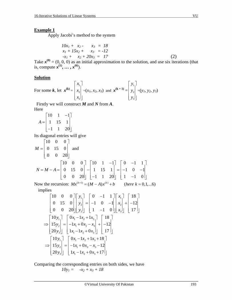
16-Iterative Solutions of Linear Systems VU
©Virtual University Of Pakistan 193
Example 1 Apply Jacobi’s method to the system
10x1 + x2 - x3 = 18 x1 + 15x2 + x3 = -12 -x1 + x2 + 20x3 = 17 (2) Take x(0) = (0, 0, 0) as an initial approximation to the solution, and use six iterations (that is, compute x(1), … , x(6)). Solution
For some k, let x(k) = 1
2
3
xxx
=(x1, x2, x3) and x(k + 1) =1
2
3
yyy
=(y1, y2, y3)
Firstly we will construct M and N from A. Here
10 1 11 15 11 1 20
A−
= −
Its diagonal entries will give 10 0 00 15 00 0 20
M =
and
10 0 0 10 1 1 0 1 10 15 0 1 15 1 1 0 10 0 20 1 1 20 1 1 0
N M A− −
= − = − = − − − −
Now the recursion: ( 1) ( )( ) ( 0,1,...6)k kMx M A x b here k+ = − + = implies
1 1
2 2
3 3
10 0 0 0 1 1 180 15 0 1 0 1 120 0 20 1 1 0 17
y xy xy x
− = − − + − −
1 1 2 3
2 1 2 3
3 1 2 3
10 0 1 1 1815 1 0 1220 1 1 0 17
y x x xy x x xy x x x
− + ⇒ = − + − + − − +
1 1 2 3
2 1 2 3
3 1 2 3
10 0 1 1 1815 1 0 1220 1 1 0 17
y x x xy x x xy x x x
− + + ⇒ = − + − − − + +
Comparing the corresponding entries on both sides, we have
10y1 = -x2 + x3 + 18

16-Iterative Solutions of Linear Systems VU
©Virtual University Of Pakistan 194
15y2 = -x1 - x3 – 12 20y3 = x1 – x2 + 17
And
y1 = (- x2 + x3 + 18)/10 y2 = ( - x1 – x3 – 12)/15 (3) y3 = (x1 – x2 + 17)/20
1st Iteration For k = 0, put x (0) = (x1, x2, x3) = (0, 0, 0) in (3) and compute x (1) = (y1, y2, y3) = (18/10, – 12/15, 17/20) = (1.8, -0.8, 0.85) 2nd Iteration For k = 1, put x (1) =(1.8, -.8, .85) y1 = [ - ( -0.8) + (0.85) + 18]/10 = 1.965 y2 = [ - (1.8) – (0.85) – 12]/15 = -0.9767 y3 = [(1.8) – (-0.8) + 17]/20 = 0.98 Thus, x (2) = (1.965, -.9767, .98). The entries in x (2) are used on the right in (3) to compute the entries in x (3), and so on. Here are the results, with calculations using MATLAB and results reported to four decimal places:
(0) (1) (2) (3) (4) (5) (6)
0 1.8 1.965 1.9957 1.9993 1.9999 2.00000 .8 .9767 .9963 .9995 .9999 1.00000 .85 .98 .9971 .9996 .9999 1.0000
x x x x x x x
− − − − − −
If we decide to stop when the entries in x (k) and x (k – 1) differ by less than .001, then we need five iterations (k = 5). Alternative Approach If we express the above system as
10x1 + x2 - x3 = 18 2 31
1810x xx − +
⇒ =
x1 + 15x2 + x3 = -12 1 32
1215
x xx − − −⇒ =
-x1 + x2 + 20x3 = 17 1 23
1720x xx + −
⇒ =
∴the equivalent system is

16-Iterative Solutions of Linear Systems VU
©Virtual University Of Pakistan 195
Now put (x1,x2,x3)=(0,0,0)= x(0) in the RHS to have x1=(18-0+0)/10 = 1.80 x2= (-12-0-0)/15 = -0.80 x3 = (17+0-0)/20 = 0.85 Which gives x(1) = (1.80,-0.80,0.85) ----put this again on RHS of the equivalent system to get x1=(18+0.80+0.85)/10 =1.965 x2= (-12-1.80-0.85)/15 = -0.9767 x3= (17+1.80+0.80)/20 = 0.98 So in the similar fashion, we can get the next approximate solutions: x(3),x(4) ,x(5) and x(6)
Next example will be solved by following this approach. Example 2 Use Jacobi iteration to approximate the solution of the system
1 2 3
1 2 3
1 2 3
20 x + x x =17x 10x + x =13
x + x + 10x =18
−−
−
Stop the process when the entries in two successive iterations are the same when rounded to four decimal places. Solution As required for Jacobi iteration, we begin by solving the first equation for x1, the second for x2, and the third for x3. This yields
1 2 3 2 3
2 1 3 1 3
3 1 2 1 2
17 1 1 0.85 0.05 0.0520 20 20
13 1 1 1.3 0.1 0.110 10 10
18 1 1 1.8 0.1 0.110 10 10
x x x x x
x x x x x
x x x x x
= − + = − +
= − + + = − + +
= + − = + −
(4)
which we can write in matrix form as 1 1
2 2
3 3
0 0.05 0.05 0.850.1 0 0.1 1.30.1 0.1 0 1.8
x xx xx x
− = + − −
(5)
2 31
1 32
1 23
1810
1215
1720
x xx
x xx
x xx
− +=
− − −=
+ −=

16-Iterative Solutions of Linear Systems VU
©Virtual University Of Pakistan 196
Since we have no special information about the solution, we will take the initial approximation to be 1 2 3 0x x x= = = . To obtain the first iterate, we substitute these values into the right side of (5). This yields
0.851.3
1.8y
= −
1
To obtain the second iterate, we substitute the entries of y1 into the right side of (5). This yields
1
2
3
0 0.05 0.05 0.85 0.85 1.0050.1 0 0.1 1.3 1.3 1.0350.1 0.1 0 1.8 1.8 2.015
xy x
x
− = = − + − = − −
2
Repeating this process until two successive iterations match to four decimal places yields the results in the following table: y0 y1 y2 y3 y4 y5 y6 y7 x1 0 0.8500 1.0050 1.0025 1.0001 1.0000 1.0000 1.0000 x2 0 -1.3000 -1.0350 -0.9980 -0.9994 -1.0000 -1.0000 -1.0000 x3 0 1.8000 2.0150 2.0040 2.0000 1.9999 2.0000 2.0000 The Gauss-Seidel Method This method uses the recursion (1) with M the lower triangular part of A. That is, M has the same entries as A on the diagonal and below, and M has zeros above the diagonal. See Fig. 1. As in Jacobi’s method, the diagonal entries of A must be nonzero in order for M to be invertible.
* * * * * * 0 0 0 0* * * * * * * 0 0 0* * * * * * * * 0 0* * * * * * * * * 0* * * * * * * * * *
A M
= =
Figure 01:The Lower Triangular Part of A Example 3 Apply the Gauss – Seidel method to the system in Example 1 with x (0) =(0,0,0) and six iterations.
10x1 + x2 - x3 = 18 x1 + 15x2 + x3 = -12 -x1 + x2 + 20x3 = 17 (6)
Solution

16-Iterative Solutions of Linear Systems VU
©Virtual University Of Pakistan 197
For some k, let x(k) = 1
2
3
xxx
=(x1, x2, x3) and x(k + 1) =1
2
3
yyy
=(y1, y2, y3)
Again, firstly we construct matrices M and N from the coefficient matrix A.
Here 10 1 11 15 11 1 20
A−
= −
Since matrix M is constructed by 1) taking the values along the diagonal and below the diagonal of coefficient matrix A. 2) putting the zeros above the diagonal at upper trianular position.
So 10 0 01 15 01 1 20
M = −
Now, 10 0 0 10 1 1 0 1 11 15 0 1 15 1 0 0 11 1 20 1 1 20 0 0 0
N M A− −
= − = − = − − −
Now the recursion: ( 1) ( )( ) ( 0,1,...6)k kMx M A x b here k+ = − + = implies
1 1
2 2
3 3
10 0 0 0 1 1 181 15 0 0 0 1 121 1 20 0 0 0 17
y xy xy x
− = − + − −
1 2 3
1 2 3
1 2 3
10 0 0 1815 0 12
20 0 17
y x xy y xy y y
− + ⇒ = − + − −
1 2 3
1 2 3
1 2 3
10 0 0 1815 0 12
20 0 17
y x xy y xy y y
− + + ⇒ = − − − +
Comparing the corresponding entries on both sides, we have
10y1 = -x2 + x3 + 18 y1+15y2 = - x3 – 12 -y1 + y2 + 20y3 =17
This further implies as

16-Iterative Solutions of Linear Systems VU
©Virtual University Of Pakistan 198
1 1 3 1 2 3
1 2 3 2 1 3
1 2 3 3 1 2
10 18 ( 18) /1015 12 ( 12) /15
20 17 ( 17) / 20
y x x y x xy y x y y x
y y y y y y
= − − + ⇒ = − + + + = − − ⇒ = − − − − + + = ⇒ = − +
-----------(7)
Another way to view (7) is to solve each equation in (6) for x1, x2, x3, respectively and regard the highlighted x’s as the values:
x1 = (- x2 + x3 + 18)/10 x2 = ( - x1 – x3 – 12)/15 x3 = (x1 – x2 + 17)/20 (8)
Use the first equation to calculate the new x1 [called y1 in (7)] from x2 and x3. Then, use this new x1 along with x3 in the second equation to compute the new x2. Finally, in the third equation, use the new values for x1 and x2 to compute x3. In this way, the latest information about the variables is used to compute new values. [A computer program would use statements corresponding to the equations in (8).] From x (0) = (0, 0, 0), we obtain x1 = [ - (0) + (0) + 18]/10 = 1.8
x2 = [ - (1.8) – (0) – 12]/15 = -.92
x3 = [+(1.8) – (-.92) + 17]/20 = .986 Thus, x (1) = (1.8, -.92, .986). The entries in x (1) are used in (8) to produce x (2) and so on. Here are the MATLAB calculations reported to four decimal places:
(0) (1) (2) (3) (4) (5) (6)
0 1.8 1.9906 1.9998 2.0000 2.0000 2.00000 .92 .9984 .9999 1.0000 1.0000 1.00000 .986 .9995 1.0000 1.0000 1.0000 1.0000
x x x x x x x
− − − − − −
Observe that when k is 4, the entries in x (4) and x (k – 1) differ by less than .001. The values in x (6) in this case happen to be accurate to eight decimal places. Alternative Approach If we express the above system as 10x1 + x2 - x3 = 18 ⇒ x1 = (- x2 + x3 + 18)/10 ------(a) x1 + 15x2 + x3 = -12 ⇒ x2 = ( - x1 – x3 – 12)/15------(b) -x1 + x2 + 20x3 = 17⇒ x3 = (x1 – x2 + 17)/20 ------(c) Ist Iteration Put x2=x3 =0 in (a)

16-Iterative Solutions of Linear Systems VU
©Virtual University Of Pakistan 199
x1= 18/10 =1.80 Put x1=1.80 and x3=0 in (b) x2 = (-1.80-0-12)/15= -0.92 Put x1=1.80, x2 = -0.92 in (c) x3=(1.80+0.92+17)/20 = 0.9863
So, (1)
1 1.82 .923 .986
xx xx
= − =
2nd iteration Put x2 = -0.92, x3=0.9863 in (a) x1=(0.92+0.9863+18)/10 = 1.9906 Put x1=1.9906(from 2nd iteration) and x3=0.9863(from 1st iteration) in (b) x2=(-1.9906-0.9863-12)/15 = -0.9984 Put x1=1.9906, x2=-0.9984(both from 2nd iteration) in (c) x3=(1.9906+0.9984+17)/20 = 0.9995
So, (2)
1 1.99062 .99843 .9995
xx xx
= − =
So in the similar fashion, we can get the next approximate solutions: x(3),x(4) ,x(5) and x(6)
Next example will be solved by following this approach. Example 4 Use Gauss-Seidel to approximate the solution of the linear system in example 2 to four decimal places. Solution As before, we will take 1 2 3 0x x x= = = as the initial approximation. First, we will substitute x2 = 0 and x3 = 0 into the right side of the first equation of (4) to obtain the new x1. Then, we will substitute x3 = 0 and the new x1 into the right side of the second equation to obtain the new x2, and finally, we will substitute the new x1 and new x2 into the right side of the third equation to obtain the new x3. The computations are as follows:
1
2
3
0.85 (0.05)(0) (0.05)(0) 0.851.3 (0.1)(0.85) (0.1)(0) 1.215
1.8 (0.1)(0.85) (0.1)( 1.215) 2.0065
xxx
= − + == − + + = −= + − − =
Thus, the first Gauss-Seidel iterate is
1
0.85001.2150
2.0065y
= −
Similarly, the computations for second iterate are

16-Iterative Solutions of Linear Systems VU
©Virtual University Of Pakistan 200
1
2
3
0.85 (0.05)( 1.215) (0.05)(2.0065) 1.0110751.3 (0.1)(1.011075) (0.1)(2.0065) 0.9982425
1.8 (0.1)(1.011075) (0.1)( 0.9982425) 2.00093175
xxx
= − − + == − + + = −= + − − =
Thus, the second Gauss-Seidel iterate to four decimal places is
2
1.01110.9982
2.0009y
≈ −
The following table shows the first four Gauss-Seidel iterates to four decimal places. Comparing both tables, we see that the Gauss-Seidel method produced the solution to four decimal places in four iterations whereas, the Jacobi method required six. y0 y1 y2 y3 y4 x1 0 0.8500 1.0111 1.0000 1.0000 x2 0 -1.2150 -0.9982 -0.9999 -1.0000 x3 0 2.0065 2.0009 2.0000 2.0000 Comparison of Jacobi’s and Gauss-Seidel method There exist examples where Jacobi’s method is faster than the Gauss-Seidel method, but usually a Gauss-Seidel sequence converges faster (means to say iterative solution approaches to the unique solution), as in Example 2. (If parallel processing is available, Jacobi might be faster because the entries in x(k) can be computed simultaneously.) There are also examples where one or both methods fail to produce a convergent sequence, and other examples where a sequence is convergent, but converges too slowly for practical use. Condition for the Convergence of both Iterative Mthods Fortunately, there is a simple condition that guarantees (but is not essential for) the convergence of both Jacobi and Gauss-Seidel sequences. This condition is often satisfied, for instance, in large-scale systems that can occur during numerical solutions of partial differential equations (such as Laplace’s equation for steady-state heat flow). An n n× matrix A is said to be strictly diagonally dominant if the absolute value of each diagonal entry exceeds the sum of the absolute values of the other entries in the same row. In this case it can be shown that A is invertible and that both the Jacobi and Gauss-Seidel sequences converge to the unique solution of Ax = b, for any initial (0)x . (The speed of the convergence depends on how much the diagonal entries dominate the corresponding row sums.) The coefficient matrices in Examples 1 and 2 are strictly diagonally dominant, but the following matrix is not. Examine each row:

16-Iterative Solutions of Linear Systems VU
©Virtual University Of Pakistan 201
6 2 31 4 23 5 8
− − − −
6 2 3
4 1 2
8 3 5
− > + −
> + −
= + −
The problem lies in the third row, because 8 is not larger than the sum of the magnitudes of the other entries. Note The practice problem below suggests a TRICK(rearrangement of the system of equations) that sometimes works when a system is not strictly diagonally dominant. Example 5 Show that the Gauss-Seidel method will produce a sequence converging to the solution of the following systems, provided the equations are arranged properly:
x1 – 3x2 + x3 = –2 –6x1 + 4x2 + 11x3 = 1
5x1 – 2x2 – 2x3 = 9 Solution The system is not strictly diagonally dominant, as for the 1st row
1 2 3
1 3 1
coefficient of x coefficient of x coefficient of x
or
< +
< − +
so neither Jacobi nor Gauss- Seidel is guaranteed to work. In fact, both iterative methods produce sequences that fail to converge, even though the system has the unique solution x1 = 3, x2 = 2, x3 = 1. However, the equations can be rearranged as
5x1 – 2x2 – 2x3 = 9 x1 – 3x2 + x3= –2 –6x1 + 4x2 + 11x3 = 1
So, for 1st equation (row);
1 2 3
5 2 2
coefficient of x coefficient of x coefficient of x
or
> +
> − + −
for 2nd equation(row); 2 1 3
3 1 1
coefficient of x coefficient of x coefficient of x
or
> +
− > +
for 3rd equation(row); 3 1 2
11 6 4
coefficient of x coefficient of x coefficient of x
or
> +
> − +
Now the coefficient matrix is strictly diagonally dominant, so we know Gauss-Seidel works with any initial vector. In fact, if x(0) = 0, then x(8) = (2.9987, 1.9992, .9996).

16-Iterative Solutions of Linear Systems VU
©Virtual University Of Pakistan 202
Exercises Solve the system in exercise 1 to 3 using Jacobi’s method, with x(0) = 0 and three iterations. Repeat the iterations until two successive approximations agree within a tolerance of .001 in each entry.
1. 1 2
1 2
4 75 7
x xx x+ =
− + = − 2. 1 2
1 2
10 258 43
x xx x
− =+ =
3. 1 2
1 2 3
2 3
3 115 2 153 7 17
x xx x x
x x
+ =− − + =
+ = 4.
1 2
1 2 3
2 3
50 149100 2 101
2 50 98
x xx x x
x x
− =− + = −
+ = −
In exercises 5 to 8, use the Gauss Seidel method, with x(0) = 0 and two iterations. Compare the number of iterations needed by Gauss Seidel and Jacobi to make two successive approximations agree within a tolerance of .001. 5. The system in exercise 1 6. The system in exercise 2 7. The system in exercise 3 8. The system in exercise 4 Determine which of the matrices in exercises 9 and 10 are strictly diagonally dominant.
9. (a) 5 44 3
(b) 9 5 25 8 12 1 4
− − − −
10. (a) 3 22 3
−
(b) 5 3 13 6 41 4 7
− −
Show that the Gauss Seidel method will produce a sequence converging to the solution of the following system, provided the equations are arranged properly:
11. 1 2 3
1 2 3
1 2 3
3 26 4 11 1
5 2 2 9
x x xx x xx x x
− + = −− + + =
− − =
12. 1 2 3
1 2
2 3
4 34 10
4 6
x x xx x
x x
− + − =− =− + =

17-Introduction to Determinant VU
©Virtual University Of Pakistan 203
Lecture 17 Introduction to Determinant In algebra, the determinant is a special number associated with any square matrix. As we have studied in earlier classes, that the determinant of 2 x 2 matrix is defined as the product of the entries on the main diagonal minus the product of the entries off the main diagonal. The determinant of a matrix A is denoted by det (A) or |A|
For example: a b
Ac d
=
Then det (A) = ad-bc. or |A| = ad – bc
Example Find the determinant of the matrix 1 23 4
A =
1 2
| | 1 4 2 3 4 6 23 4
A = = × − × = − =−
To extend the definition of the det(A) to matrices of higher order, we will use subscripted entries for A.
11 12
21 22
a aA
b b
=
det (A) = 11 1211 22 12 21
21 22
a aa b a b
b b= −
This is called a 2x2 determinant. The determinant of a 3x3 matrix is also called a 3x3 determinant is defined by the following formula.
11 12 13
21 22 23
31 32 33
a a aa a aa a a
(1)
For finding the determinant of the 3x3 matrix, we look at the following diagram:
11 12 13 11 12
21 22 23 21 22
31 32 33 31 32
a a a a aa a a a aa a a a a

17-Introduction to Determinant VU
©Virtual University Of Pakistan 204
We write 1st and 2nd columns again beside the determinant. The first arrow goes from a11 to a33, which gives us product: 11 22 33 a a a . The second arrow goes from a12 to a31,
which gives us product: 12 23 31a a a . The third arrow goes from a13 to a32, which gives us the product: 13 21 32a a a . These values are taken with positive signs. The same method is used for the next three arrows that go from right to left downwards, but these products are taken as negative signs.
11 22 33+ 12 23 31+ 13 21 32 13 22 31 11 23 32 12 21 33= a a a a a a a a a - a a a - a a a - a a a
Example 2 Find the determinant of the matrix1 2 34 5 6
7 8 9A
= − −
1 2 3detA= -4 5 6
7 -8 9
1 2 3 1 2 = -4 5 6 -4 5
7 -8 9 7 -8
= 1 5 9 + 2 6 7 + 3 (-4) (-8)- 3 5 7 -1 6 (-8)- 2 (-4) 9× × × × × × × × × × × ×
= 45+84+96 -105+48+72= 240
We saw earlier that a 2 2× matrix is invertible if and only if its determinant is nonzero. In simple words, a matrix has its inverse if its determinant is nonzero. To extend this useful fact to larger matrices, we need a definition for the determinant of the n n× matrix. We can discover the definition for the 3 3× case by watching what happens when an invertible3 3× matrix A is row reduced. Gauss’ algorithm for evaluation of determinants 1) Firstly, we apply it for 2 2× matrix say
2 34 3
A =
2 2 12R R R′ → − (Multiplying 1st row by 2 and then subtracting from 2nd row) 2 3 2 3
4 2(2) 3 2(3) 0 3
= − − −
Now the determinant of this upper triangular matrix is the product of its entries on main diagonal that is

17-Introduction to Determinant VU
©Virtual University Of Pakistan 205
( ) 2( 3) 0 3 6 0 6Det A = − − × = − − =− 2) For 3 3× matrix say
2 2 31 1 3
2 0 1B
− − = − −
12 21By R R′ → (Interchanging of 1st and 2nd rows)
2 2 12R R R′ → − (Multiplying 1st row by ‘-2’ and then adding in the 2nd row)
3 3 12R R R′ → + (Multiplying 1st row by ‘2’ and then adding in the 3rd row) 1 1 3
0 0 90 2 5
− −
23 32By R R′ → (Interchanging of 2nd and 3rd rows) 1 1 3
0 2 50 0 9
− −
Now the determinant of this upper triangular matrix is the product of its entries on main diagonal and that is
( ) ( 1) 2 ( 9) 18Det B = − ⋅ ⋅ − = So in general, For a 1 1× matrix say, [ ]ijA a= - we define 11det A a= . For 2 2× matrix
11 12
21 22
a aa a
By 212 2 1
11
aR R Ra
′ → −
provided that 11 0a ≠
11 12
2122 12
11
0
a aaa aa
−
∴ det A∆ = = product of the diagonal entries
1 1 32 2 3
2 0 1
− − − −

17-Introduction to Determinant VU
©Virtual University Of Pakistan 206
2111 22 12 11 22 12 21
11
aa a a a a a aa
= − = −
For 3 3× matrix say
11 12 13
21 22 23
31 32 33
a a aa a aa a a
By 31212 2 1 3 3 1
11 11
, aaR R R R R Ra a
′ ′→ − → −
provided that 11 0a ≠
11 12 13
23 11 13 2122 11 12 21
11 11
32 11 12 31 11 33 13 31
11 11
0
0
a a aa a a aa a a a
a aa a a a a a a a
a a
−− − −
By
32 11 12 31
113 3 2
22 11 12 21
11
a a a aaR R Ra a a aa
−
′ → −−
provided that 22 11 12 21
11
0a a a aa−
≠
11 1213
23 11 13 2122 11 12 2111
11 11
32 11 12 31
11 33 13 31 23 11 13 21 11
22 11 12 2111 11
11
0 0
0 0
a a a
a a a aa a a a aa a
a a a aa a a a a a a a a
a a a aa aa
−− ≠
− − − / − − /
Which is in echelon form.Now,
det A∆ = = product of the diagonal entries

17-Introduction to Determinant VU
©Virtual University Of Pakistan 207
( ) ( )
11 33 13 31 23 11 13 21 32 11 12 3122 11 12 2111
11 11 11 22 11 12 21
11 33 13 31 23 11 13 21 32 11 12 3122 11 12 21 22 11 12 21
11 11 22 11
a a a a a a a a a a a aa a a aaa a a a a a a
a a a a a a a a a a a aa a a a a a a aa a a a a
− − −−= −/ −/
− − −= − − − −
( )( ) ( )( ){ }
{ }
12 21
22 11 12 21 11 33 13 31 23 11 13 21 32 11 12 3111
2 211 22 33 11 22 13 31 12 21 11 33 12 21 13 31 23 11 32 23 11 12 31 13 21 32 11 12 21 13 31
11
211 22 33 11 22 13 3
11
1
1
1
a
a a a a a a a a a a a a a a a aa
a a a a a a a a a a a a a a a a a a a a a a a a a a a a a aa
a a a a a a aa
= − − − − −
= − − + − + + −
= −{ }
{ }
21 12 21 11 33 23 11 32 23 11 12 31 13 21 32 11
1111 22 33 22 13 31 12 21 33 23 11 32 23 12 31 13 21 32
11
11 22 33 12 23 31 13 21 32 12 21 33 11 23 32 13 22 31
a a a a a a a a a a a a a a a
a a a a a a a a a a a a a a a a a a aaa a a a a a a a a a a a a a a a a a
− − + +
= − − − + +
= + + − − − Since A is invertible, ∆ must be nonzero. The converse is true as well. To generalize the definition of the determinant to larger matrices, we will use 2 2× determinants to rewrite the 3 3× determinant ∆ described above. Since the terms in ∆ can be grouped as:
11 22 33 11 23 32 12 23 31 12 21 33 13 21 32 13 22 31
11 22 33 23 32 12 21 33 23 31 13 21 32 22 31
( ) ( ) ( )( ) ( ) ( )
a a a a a a a a a a a a a a a a a aa a a a a a a a a a a a a a a
∆ = − − − + −= − − − + −
,
22 23 21 23 21 2211 12 13
32 33 31 33 31 32
det det deta a a a a a
a a aa a a a a a
∆ = ⋅ − ⋅ + ⋅
22 23 21 23 21 2211 12 13
32 33 31 33 31 32
a a a a a aa a a
a a a a a a∆ = ⋅ − + ⋅
For brevity, we write 11 11 12 12 13 13det det deta A a A a A∆ = ⋅ − ⋅ + ⋅ (3)
22 2311
32 33
det( )a a
Aa a
= , 21 2312
31 33
det( )a a
Aa a
= and 21 2213
31 32
det( )a a
Aa a
=
where A11 is obtained from A by deleting the first row and first column. A12 is obtained from A by deleting the first row and second column. A13 is obtained from A by deleting the first row and third column. So in general, for any square matrix A, let Aij denote the sub-matrix formed by deleting the ith row and jth column of A. Let’s understand it with the help of an example.
17-Introduction to Determinant VU
©Virtual University Of Pakistan 208
Example3
Find the determinant of the matrix1 4 35 2 43 6 3
A =
Solution Given 1 4 35 2 43 6 3
A =
1 4 3| | 5 2 4
3 6 3
2 4 5 4 5 21 4 3
6 3 3 3 3 61(2 3 4 6) 4(5 3 4 3) 3(5 6 2 3)1(6 24) 4(15 12) 3(30 6)1( 18) 4(3) 3(24)
18 12 7242
A =
= − +
= × − × − × − × + × − ×= − − − + −= − − += − − +=
For instance, if 1 -2 5 02 0 4 -1=3 1 0 70 4 -2 0
A
then A32 is obtained by crossing out row 3 and column 2,
1 2 5 02 0 4 13 1 0 70 4 2 0
− − −
so that 32
1 5 02 4 10 2 0
A = −
−
We can now give a recursive definition of a determinant. When n = 3, det A is defined using determinants of the 2 2× submatrices 1 jA . When n = 4, det A uses determinants of the3 3× submatrices 1 jA In general, an nxn determinant is defined by determinants of ( 1) ( 1)n n− × − sub matrices.

17-Introduction to Determinant VU
©Virtual University Of Pakistan 209
Definition For 2,n ≥ the determinant of n n× matrix [ ]ijA a= is the sum of n terms of the form
1 1(det )j ja A± × , with plus and minus signs alternating, where the entries 11 12 1, , , na a a are from the first row of A. Here for ija ,
1, 2,3, , (1 )1,2,3, , (1 )
i n i nj n j n= ≤ ≤= ≤ ≤
In symbols, 111 11 12 12 1 1det det det .... ( 1) detn
n nA a A a A a A+= − + + − 11 1
1( 1) det
nj
j jj
a A+
=
= −∑
Example 4
Compute the determinant of 1 5 02 4 10 2 0
A = − −
Solution Here A is 3 3n n× = × matrix such that 1, 2,3i =
1, 2,3j = 1
1 11
det( ) ( 1) detn
jj j
jA a A+
== −∑ and here 1,2,3j =
31 1 1 1 2 1 3
1 1 11 11 12 12 13 131
det( ) ( 1) det ( 1) det ( 1) det ( 1) detjj j
jA a A a A a A a A+ + + +
=
∴ = − = − + − + −∑
= 11 11 12 12 13 13det det deta A a A a A− +
4 1 2 1 2 4det 1.det 5.det 0.det
2 0 0 0 0 2A
− − = − + − −
4 1 2 1 2 4
det 1. 5. 0.2 0 0 0 0 2
A− −
= − +− −
= 1 [4(0) – (-1)(-2)] -5 [ 2(0) – 0(-1)] +0[2(-2) – 4(0)]
1(0 2) 5(0 0) 0( 4 0) 2= − − − + − − = − Minor of an element If A is a square matrix, then the Minor of entry aij (called the ijth minor of A) is denoted by Mij and is defined to be the determinant of the sub matrix that remains when the ith row and jth column of A are deleted.

17-Introduction to Determinant VU
©Virtual University Of Pakistan 210
In the above example, Minors are as follows:
11 12 13, ,4 1 2 1 2 42 0 0 0 0 2M MM = = =
− −− −
Cofactor of an element The number Cij=(-1)i+jMij is called the cofactor of entry aij(or the ijth cofactor of A). When the + or – sign is attached to the Minor, then Minor becomes a cofactor. In the above example, following are the Cofactors:
111 1 1 2 1 3
11 12 12 13 13
1 1 1 2 1 311 12 13
( 1) , ( 1) , ( 1)
( 1) , ( 1) , ( 1)4 1 2 1 2 42 0 0 0 0 2
M C M C M
C C
C
C
+ + +
+ + +
= − = − = −
= − = − = −− −
− −
Example 5 Find the minor and the cofactor of the matrix3 1 42 5 61 4 8
A−
=
Solution Here 3 1 42 5 61 4 8
A−
=
The minor of entry a11 is
11
3 1 45 6
2 5 6 5 8 6 4 40 24 164 8
1 4 8M
−= = = × − × = − =
and the corresponding cofactor is 1 1
11 11 11( 1) 16C M M+= − = = The minor of entry a32 is
32
3 1 43 4
M 2 5 6 262 6
1 4 8
−−
= = =
and the corresponding cofactor is 3 2
32 32 32
3 4( 1) 26
2 6C M M+ −
= − = − = − = −

17-Introduction to Determinant VU
©Virtual University Of Pakistan 211
Alternate Definition Given [ ]i jA a= , the (i, j)-cofactor of A is the number i jC given by
( 1) deti ji j ijC A+= − (4)
Then 11 11 12 12 1 1det .... n nA a C a C a C= + + + This formula is called the cofactor expansion across the first row of A.
Example 6 Expand a 3x3 determinant using cofactor concept1 2 34 5 6
7 8 9A = −
−
Solution Using cofactor expansion along the first column;
1 1 2 1 3 1
11 21 31
2 3 4
1 2 35 6 2 3 2 3
4 5 6 (1)( 1) ( 4)( 1) (7)( 1)8 9 8 9 5 6
7 8 9
(4),
1 ( 4) 7
5 6 2 3 2 3(1)( 1) ( 4)( 1) (7)( 1)
8 9 8 9 5 6
5 6 2 3 2 3(1)(1) ( 4)( 1) (7)(1)
8 9 8 9 5 6
5 6 21 4
8 9
Nowif we compareit with the formula
C C C
+ + +− = − + − − + −− −
−
= + − +
= − + − − + −− −
= + − − +− −
= +−
3 2 37
8 9 5 6
1(45 ( 48)) 4(18 ( 24)) 7 (12 15)
1( 45 48) 4(18 24) 7 (12 15)
(1)(93) (4)(42) (7)( 3) 240
+−
= − − + − − + −
= + + + + −
= + + − =
Using cofactor expansion along the second column,

17-Introduction to Determinant VU
©Virtual University Of Pakistan 212
1 2 2 2 3 2
3 4 5
1 2 34 6 1 3 1 3
4 5 6 (2)( 1) (5)( 1) ( 8)( 1)7 9 7 9 4 6
7 8 9
4 6 1 3 1 3(2)( 1) (5)( 1) ( 8)( 1)
7 9 7 9 4 6
4 6 1 3 1 3(2)( 1) (5)(1) ( 8)( 1)
7 9 7 9 4 6
4 6 1 3 1 32 5 8
7 9 7 9 4 6
2( 36 42) 5(9 21) 8(6 ( 12))
( 2)( 78)
+ + +−− = − + − + − −
−−
−= − + − + − −
−
−= − + + − −
−
−= − + +
−
=− − − + − + − −
= − − (5)( 12) (8)(18) 240+ − + =
Theorem 1 The determinant of an n n× matrix A can be computed by a cofactor expansion across any row or down any column. The expansion across the ith row using the cofactors in (4) is
1 1 2 2det i i i i in inA a C a C a C= + + +
The cofactor expansion down the jth column is
1 1 2 2det j j j j nj njA a C a C a C= + + + The plus or minus sign in the (i, j)-cofactor depends on the position of ija in the matrix,
regardless of the sign of ija itself. The factor ( 1)i j+− determines the following checkerboard pattern of signs:
....+ − + − + − + − +
17-Introduction to Determinant VU
©Virtual University Of Pakistan 213
Example 7 Use a cofactor expansion across the third row to compute det A, where
1 5 02 4 10 2 0
A = − −
Solution Compute 31 31 32 32 33 33det A a C a C a C= + +
3 1 3 2 3 331 31 32 32 33 33( 1) det ( 1) det ( 1) deta A a A a A+ + += − + − + −
5 0 1 0 1 5
0 ( 2) 04 1 2 1 2 4
= − − +− −
0 2( 1) 0 2= + − + = −
Theorem 1 is helpful for computing the determinant of a matrix that contains many zeros. For example, if a row is mostly zeros, then the cofactor expansion across that row has many terms that are zero, and the cofactors in those terms need not be calculated. The same approach works with a column that contains many zeros.
Example 8 Evaluate the determinant of
2 0 0 51 2 4 1
3 0 0 38 6 0 0
A
− =
Solution
2 0 0 51 2 4 1
det( )3 0 0 38 6 0 0
A−
=
Expand from third column

17-Introduction to Determinant VU
©Virtual University Of Pakistan 214
13 23 33 43
23
23
2 3
det( ) 0 4 0 0
0 4 0 0
4
2 0 54 ( 1) 3 0 3
8 6 0
A C C C C
C
C
+
= × + × + × + ×
= + × + +
= ×
= × −
Expand from second column
2 54 0 0 ( 6)
3 3
2 5( 4) ( 6)
3 3
216
= − + + −
= − −
= −
Example 9 Show that the value of the determinant is independent of θ
sin cos 0cos sin 0
cos sin sin cos 1A
θ θθ θ
θ θ θ θ= −
− +
Solution Consider sin cos 0cos sin 0
cos sin sin cos 1A
θ θθ θ
θ θ θ θ= −
− +
Expand the given determinant from 3rd column we have
3 3 2 20 0 ( 1) [sin cos ] 1θ θ+= − + − + =
17-Introduction to Determinant VU
©Virtual University Of Pakistan 215
Example 10 Compute det A, where
3 7 8 9 60 2 5 7 30 0 1 5 00 0 2 4 10 0 0 2 0
A
− − − = − −
Solution The cofactor expansion down the first column of A has all terms equal to zero except the first.
Thus 21 31 41 51
2 5 7 30 1 5 0
det 3 0. 0. 0. 0.0 2 4 10 0 2 0
A C C C C
−
= − + − +−
−
Henceforth, we will omit the zero terms in the cofactor expansion. Next, expand this 4 4× determinant down the first column, in order to take advantage of the zeros there.
We have 1 5 0
det 3 2 2 4 10 2 0
A = × −−
This 3 3× determinant was computed above and found to equal –2. Hence, det A = 3 2 ( 2) 12× × − = − . The matrix in this example was nearly triangular. The method in that example is easily adapted to prove the following theorem. Triangular Matrix A triangular matrix is a special kind of m x n matrix where the entries either below or above the main diagonal are zero.
is upper triangular and 25 25× is lower triangular matrices.
Determinants of Triangular Matrices Determinants of the triangular matrices are also easy to evaluate regardless of size.

17-Introduction to Determinant VU
©Virtual University Of Pakistan 216
Theorem If A is triangular matrix, then det (A) is the product of the entries on the main diagonal. Consider a 4 4× lower triangular matrix.
11
21 22
31 32 33
41 42 43 44
0 0 00 0
0
aa a
Aa a aa a a a
=
Keeping in mind that an elementary product must have exactly one factor from each row and one factor from each column, the only elementary product that does not have one of the six zeros as a factor is 11 22 33 44( )a a a a . The column indices of this elementary product are in natural order, so the associated signed elementary product takes a +. Thus, det (A)= 11 22 33 44a a a a× × ×
Example 11 2 5 7
0 3 8 ( 2)(3)(5) 300 0 5
−= − = −
1 0 0 04 9 0 0
(1)(9)( 1)( 2) 187 6 1 0
3 8 5 2
= − − =− −
− −
1 2 7 30 1 4 1
(1)(1)(2)(3) 60 0 2 70 0 0 3
−−
= =
The strategy in the above Example of looking for zeros works extremely well when an entire row or column consists of zeros. In such a case, the cofactor expansion along such a row or column is a sum of zeros. So, the determinant is zero. Unfortunately, most cofactor expansions are not so quickly evaluated. Numerical Note By today’s standards, a 25 25× matrix is small. Yet it would be impossible to calculate a 25 25× determinant by cofactor expansion. In general, a cofactor expansion requires over n! multiplications, and 2525! 1.5 10x .

17-Introduction to Determinant VU
©Virtual University Of Pakistan 217
If a supercomputer could make one trillion multiplications per second, it would have to run for over 500,000 years to compute a 25 25× determinant by this method. Fortunately, there are faster methods, as we’ll soon discover.
Example 12 Compute
5 7 2 20 3 0 45 8 0 3
0 5 0 6
−−
− −−
Solution Take advantage of the zeros. Begin with a cofactor expansion down the third column to obtain a 3 3× matrix, which may be evaluated by an expansion down its first column,
1 3
5 7 2 20 3 4
0 3 0 4( 1) 2 5 8 3
5 8 0 30 5 6
0 5 0 6
+
−−
−= − − −
− −−
−
2 1 3 4
2 ( 1) ( 5) 205 6
+ −= ⋅ − − =
−
The –1 in the next-to-last calculation came from the position of the –5 in the3 3× determinant.

17-Introduction to Determinant VU
©Virtual University Of Pakistan 218
Exercises Compute the determinants in exercises 1 to 6 by cofactor expansions. At each step, choose a row or column that involves the least amount of computation.
1.
6 0 0 51 7 2 52 0 0 08 3 1 8
− 2.
1 2 5 20 0 3 02 6 7 55 0 4 4
−
− −
3.
3 5 8 40 2 3 70 0 1 50 0 0 2
−− −
4.
4 0 0 07 1 0 02 6 3 05 8 4 3
−
− −
5.
4 0 7 3 50 0 2 0 07 3 6 4 85 0 5 2 30 0 9 1 2
− −
− −−
−
6.
6 3 2 4 09 0 4 1 08 5 6 7 13 0 0 0 04 2 3 2 0
−−
Use the method of Example 2 to compute the determinants in exercises 7 and 8. In exercises 9 to 11, compute the determinant of elementary matrix. In exercises 12 and 13,
verify that det EA = (det E) . (det A), where E is the elementary matrix and a b
Ac d
=
.
7. 3 0 42 3 20 5 1−
8. 2 4 33 1 21 4 1
−
− 9.
1 0 00 1 00 1k
10. 0 0
0 1 00 0 1
k
11. 0 1 01 0 00 0 1
12. 10 1
k
13. 0 11 0
14. Let 3 1
.4 2
A =
Write 5A. Is det 5A = 5 det A?
15. Let a b
Ac d
=
and k be a scalar. Find a formula that relates det (kA)to k and det A.
18-Properties of Determinants VU
©Virtual University Of Pakistan 219
Lecture 18
Properties of Determinants In this lecture, we will study the properties of the determinants. Some of them have already been discussed and you will be familiar with these. These properties become helpful, while computing the values of the determinants. The secret of determinants lies in how they change when row or column operations are performed. Theorem 3 (Row Operations): Let A be a square matrix.
a. If a multiple of one row of A is added to another row, the resulting determinant will remain same.
b. If two rows of A are interchanged to produce B, then det B = –det A. c. If one row of A is multiplied by k to produce B, then det B = k . det A.
The following examples show how to use Theorem 3 to find determinants efficiently.
a. If a multiple of one row of A is added to another row, the resulting determinant will remain same.
Example
11 12 13
21 22 23
31 32 33
a a aa a aa a a
∆=
21 22 23
2 ' '1 ' '
Multiplying nd row by non zero scalar say k aska ka ka adding this in st row then A becomes
−− − − −
11 21 12 22 13 23
21 22 23 1 1 2
31 32 33
a ka a ka a kaa a a R R kRa a a
+ + +′= → +
If each element of any row(column) can be expressed as sum of two elements then the resulting determinant can be expressed as sum of two determinants, so in this case
11 12 13 21 22 23
21 22 23 21 22 23
31 32 33 31 32 33
a a a ka ka kaa a a a a aa a a a a a
∆ = +
∆11 12 13 21 22 23
21 22 23 21 22 23
31 32 33 31 32 33
a a a a a aa a a k a a aa a a a a a
= + By using property (c) of above theorem 3.
If any two rows or columns in a determinant are identical then value of this determinant is zero. So in this case 1 2R R≡

18-Properties of Determinants VU
©Virtual University Of Pakistan 220
11 12 13
21 22 23
31 32 33
11 12 13
21 22 23
31 32 33
(0)a a aa a a ka a a
a a aa a a Aa a a
∴ ∆ = +
= =
b. If two rows of A are interchanged to produce B, then det B = –det A.
Example 1
1 2 35 1 10 8 9
A =
Now,1 2 3
det 5 1 1 1(9 8) 2(45 0) 3(40 0) 1 90 120 310 8 9
A = = − − − + − = − + =
Now interchange column 1st with 2nd we get a new matrix,2 1 31 5 18 0 9
B =
2 1 3det 1 5 1 2(45 0) 1(9 8) 3(0 40) 90 1 120 31
8 0 9B = = − − − + − = − − = −
c. If one row of A is multiplied by k to produce B, then det B = k . det A.
1 2 35 0 10 8 9
1(0 8) 2(45 0) 3(40 0)8 90 120 22
A
A
=
= − − − + −
=− − + =
1 ,1 2 35 0 10 8 9
MultiplingR by k we get sayk k k
B =

18-Properties of Determinants VU
©Virtual University Of Pakistan 221
(40 0) 2 (45 0) 3 (40 0)B k k k= − − − + − 40 90 120 22k k k kk A
= − + =
=
Example 2
Evaluate
1 2 3 42 3 4 13 4 1 24 1 2 3
A
=
Solution 1 2 3 42 3 4 1
det3 4 1 24 1 2 3
A =
2 2 1 3 3 1 4 4 1
1 2 3 40 1 2 7
( 2) , ( 3) , ( 4)0 2 8 100 7 10 13
by R R R R R R R R R− − − ′ ′ ′= → + − → + − → + −− − −− − −
( )
2 2 1 3 3 1
1 2 72 8 10 expanding from Ist column7 10 13
1 2 7( 1)( 2)( 1) 1 4 5 ( 1), ( 2) 1 1 ,2 ,3
7 10 13
1 2 7( 2) 0 2 2 ( 1) , ( 7)
0 4 36
2 2( 2) expanding by1st column
4 36
( 2)(2
taking and common from st nd rd rows
by R R R R R R
− − −= − − −
− − −
= − − − − − −
′ ′= − − → + − → + −− −
−= −
− −
= −
2 1
1 1)( 4) taking 2and (-4)common from1st and 2nd rows respectively.
1 9
1 116 ( 1)
0 10160
by R R
−−
−= + −
=

18-Properties of Determinants VU
©Virtual University Of Pakistan 222
Example 3 Evaluate the determinant of the matrix
4 2 5 101 1 6 37 3 0 50 2 5 8
A
=
Solution 4 2 5 101 1 6 3
det7 3 0 50 2 5 8
A =
1 2 12
1 1 6 34 2 5 10
interchanging ( )7 3 0 50 2 5 8
R and R R′= −
2 2 1 3 3 1
1 1 6 30 2 19 2
( 4) , ( 7)0 4 42 160 2 5 8
By R R R R R R− − − ′ ′= − → + − → + −− − −
2 19 24 42 16 expanding from 1st column
2 5 8
− − −= − − − −
31 2
2 19 2=(-1) 4 42 16 taking (-1)as a common factor from R and R
2 5 8
2 19 24 42 162 5 8
= −
1 19 22 2 42 16
1 5 8= −
2 2 1 3 3 1
1 19 2( 2) 0 4 12 ( 2) , ( 1)
0 14 6By R R R R R R′ ′= − → + − → + −
−

18-Properties of Determinants VU
©Virtual University Of Pakistan 223
2 1 3 1
1 19 2( 2) 0 4 12 ( 2) , ( 1)
0 14 6R R R R= − + − + −
−
4 122 expand from Ist column
14 6= 2(24+168)= 384
= −−
− −
Example 4 Without expansion, show that 0x a x b cx b x c ax c x a b
+ ++ + =+ +
Solution
2 2 1
1' '111
x a x b cx b x c ax c x a b
x a x x b cx b x x c a By C C Cx c x x a b
x a b cx b c ax c a b
Taking x common fromCa b c
x b c ac a b
+ ++ ++ +
+ − +′= + − + → −
+ − +
+= +
+
+= +
+
2 2 3
111
a b c b cx b c a c a By C C C
c a b a b
+ + +′= + + + → +
+ + +
Now taking (a+b+c) common form C2
1 2
1 1( ) 1 1
1 10 as column Ist and 2nd are identical (C C ). So its value will be zero.
b cx a b c c a
a b
+= + + +
+
= ≡
18-Properties of Determinants VU
©Virtual University Of Pakistan 224
Example 5 Evaluate
2 3 1 0 11 1 3 1 22 1 2 3 43 2 1 1 24 1 1 0 0
A =
Solution Interchanging R1 and R2, we get 1 1 3 1 22 3 1 0 1
A=- 2 1 2 3 43 2 1 1 24 1 1 0 0
2 2 1 3 3 1 4 4 1 5 5 12 , 2 , 3 , 41 1 3 1 20 1 5 2 30 1 4 1 00 1 8 2 40 3 11 4 8
R R R R R R R R R R R R′ ′ ′ ′→ → → →− − − −
− − −= − − −
− − − −− − − −
expand from C11 5 2 31 4 1 01 8 2 43 11 4 8
− − −− −
= −− − − −− − − −
2 2 1 3 3 1 4 4 1, , 31 5 2 30 9 1 30 13 4 70 26 10 17
R R R R R R R R R′ ′ ′→ → →+ + +− − −− − −
= −− − −− − −
expand from C19 1 313 4 726 10 17
− − −= − − − −
− − −

18-Properties of Determinants VU
©Virtual University Of Pakistan 225
taking (-1) common from Ist,2nd and 3rd row9 1 3
= 13 4 726 10 17
12interchange Ist and 2nd Column(C )1 9 3
= 4 13 710 26 17
−
′
2 2 1 3 3 19 , 31 0 04 23 5
10 64 13expand from Ist row
-23 -5=- (299 320) 21
-64 -13
C C C C C C′ ′→ − → −
= − − −− −
= − − =
An Algorithm to evaluate the determinant Algorithm means a sequence of a finite number of steps to get a desired result. The word Algorithm comes from the famous Muslim mathematician AL-Khwarizmi who invented the word algebra. The step-by-step evaluation of det(A) of order n is obtained as follows: Step 1: By an interchange of rows of A (and taking the resulting sign into account) bring a non zero entry to (1,1) the position (unless all the entries in the first column are zero in which case det A=0). Step 2: By adding suitable multiples of the first row to all the other rows, reduce the (n-1) entries, except (1,1) in the first column, to 0. Expand det(A) by its first column. Repeat this process or continue the following steps. Step 3: Repeat step 1 and step 2 with the last remaining rows concentrating on the second column. Step 4: Repeat step 1,step2 and step 3 with the remaining (n-2) rows, (n-3) rows and so on, until a triangular matrix is obtained. Step5: Multiply all the diagonal entries of the resulting triangular matrix and then multiply it by its sign to get det(A)

18-Properties of Determinants VU
©Virtual University Of Pakistan 226
Example 6 Compute det A, where1 4 22 8 91 7 0
A−
= − − −
.
Solution The strategy is to reduce A to echelon form and then to use the fact that the determinant of a triangular matrix is the product of the diagonal entries. The first two row replacements in column 1 do not change the determinant:
2 2 1 3 1 3
1 4 2det 2 8 9
1 7 0
1 4 20 0 5 2 ,0 3 2
A
By R R R R R R
−= − −−
−′ ′= − → + → +
An interchange of rows 2 and 3 ( 23R′ ), it reverses the sign of the determinant, so 1 4 2
det 0 3 2 (1)(3)( 5) 150 0 5
A−
= − = − − =−
Example 7 Compute det A, where
2 8 6 83 9 5 103 0 1 2
1 4 0 6
A
− − = − − −
.
Solution Taking’2’ common from 1st row
2 2 1 3 3 1 4 4 1
1 4 3 40 3 4 2
det 2 3 , 3 ,0 0 6 20 0 3 2
A By R R R R R R R R R
−− −
′ ′ ′= → − → + → −−−
1 4 3 43 9 5 10
det 23 0 1 2
1 4 0 6
A
−−
=− −
−
18-Properties of Determinants VU
©Virtual University Of Pakistan 227
14 4 32
1 4 3 40 3 4 2
det 2 ( )0 0 6 20 0 0 1
2.{(1)(3)( 6)(1)} 36
A By R R R
−− −
′= → −−
= − = −
Example 8 Show that 3
2 2 22 2 2
( 6)( 2)2 2 22 2 2
xx
x xx
x
= + −
Solution
1 1 2 3 4
2 2 22 2 22 2 22 2 2
6 2 2 26 2 2
( )6 2 26 2 2
xx
xx
xx x
By C C C C Cx xx x
++
′= → + + +++
Taking (x+6) common from 1st column 1 2 2 21 2 2
( 6)1 2 21 2 2
xx
xx
= +
2 2 1 3 3 1 4 4 1
1 2 2 20 2 0 0
( 6) , ,0 0 2 00 0 0 2
xx By R R R R R R R R R
xx
−′ ′ ′= + → − → − → −
−−
And this is the triangular matrix and its determinant is the prodcut of main diagonal’s entries.
3( 6)( 2)x x= + −

18-Properties of Determinants VU
©Virtual University Of Pakistan 228
Example 9 Compute det A, where
3 1 2 50 5 3 66 7 7 45 8 0 9
A
− − − − = − − − −
.
Solution
3 1 2 50 5 3 66 7 7 45 8 0 9
A
− − − − = − − − −
3 3 1
3 1 2 50 5 3 6
det 20 5 3 65 8 0 9
A R R R
− − − − ′= → + − − − −
= 0 as 2 3R R≡
Example10 Compute det A, where
0 1 2 12 5 7 30 3 6 22 5 4 2
A
− − = − − −
Solution
4 4 2
12
0 1 2 12 5 7 30 3 6 22 5 4 2
0 1 2 12 5 7 30 3 6 20 0 3 1
2 1 2 10 5 7 3
( 1)0 3 6 20 0 3 1
A
R R R
By R
− − = − − −
− − ′= → + −
− − ′= − −
Expanding from 1st row and 1st column
18-Properties of Determinants VU
©Virtual University Of Pakistan 229
( )
5 7 32 3 6 2
0 3 1
2 {5(6 6) ( 7)(3 0) 3( 9 0)}54
−=−
−
= − + − − − + − −
=
Remarks Suppose that a square matrix A has been reduced to an echelon form U by row replacements and row interchanges. If there are r interchanges, then det( ) ( 1) det( )rA U= − Furthermore, all of the pivots are still visible in U (because they have not been scaled to ones). If A is invertible, then the pivots in U are on the diagonal (since A is row equivalent to the identity matrix). In this case, det U is the product of the pivots. If A is not invertible, then U has a row of zero and det U = 0.
0 00 0 0 00 0 0 0 0 0 0
det 0 det 0
U U
U U
• • • • = = • • •
≠ =
Thus we have the following formula ( 1) .( )
det0
r Product of pivots inU When Ais invertibleA
When Ais not invertible −
=
(1)
Example Case-01 For 2×2 invertible matrix Reducing given 2×2 invertible matrix into Echelon form as follows;
4 53 2
A =
By interchanging 1st and 2nd rows( 12R′ ) 3 24 5
one replacement of rows has occurred, 1r∴ =
3 2703
By 2 2 143
R R R′ → − , we have desired row-echelon form 3 2
703
U =
.
Thus using the above formula as follows;

18-Properties of Determinants VU
©Virtual University Of Pakistan 230
1 7det ( 1) .( ) ( 1) (3 ) 73
rA Product of pivots inU= − = − ⋅ = −
Case-02 For 2×2 non-invertible matrix In this case say;
4 58 10
A =
4 50 0
2 2 12By R R R′ → − ,desired row-echelon form is 4 50 0
U =
Here no interchange of rows has occurred. So, 0r = and
0det ( 1) .( ) ( 1) (4 0) 0rA Product of pivots inU∴ = − = − ⋅ = Theorem 5 If A is an n n× matrix, then det AT = det A.
Example 11 If1 4 12 1 23 1 3
A =
, find det(A) and det (AT )
1 4 1det 2 1 2 1(3 2) 4(6 6) 1(2 3) 1 0 1 0
3 1 3A = = − − − + − = − − =
Now 1 2 34 1 11 2 3
tA =
1 2 3det 4 1 1 1(3 2) 2(12 1) 3(8 1) 1 22 21 0
1 2 3
tA = = − − − + − = − + =
Remark Column operations are useful for both theoretical purposes and hand computations. However, for simplicity we’ll perform only row operations in numerical calculations.
Theorem 6 (Multiplicative Property) If A and B are n n× matrices, then det( ) (det )(det )AB A B= .
Example 12 Verify Theorem 6 for 6 1 4 33 2 1 2
A and B = =

18-Properties of Determinants VU
©Virtual University Of Pakistan 231
Solution 6 1 4 3 25 203 2 1 2 14 13
AB = =
and det 25.13 20.14 325 280 45AB = − = − = Since det A = 9 and det B = 5, (det )(det ) 9.5 45 detA B AB= = = Remark det (A + B) ≠ det A + det B, in general. For example,
If 2 31 5
A = −
and 2 31 5
B− −
= − . Then
0 0det( ) 0
0 0
2 3 2 3det det ( 10 3) ( 10 3) 26 det( )
1 5 1 5
A B A B
A B A B
+ = ⇒ + =
− −
+ = + = − − + − − = − ≠ +− −

18-Properties of Determinants VU
©Virtual University Of Pakistan 232
Exercise Find the determinants in exercises 1 to 6 by row reduction to echelon form.
1.
1 3 0 22 5 7 4
3 5 2 11 1 2 3
− −
− −
2.
1 3 3 40 1 2 52 5 4 33 7 5 2
−−−
− − −
3.
1 1 3 00 1 5 41 2 8 5
3 1 2 3
− −
−− −
4.
1 3 1 0 20 2 4 1 62 6 2 3 9
3 7 3 8 73 5 5 2 7
− −− − −
− −− −
5.
1 2 3 15 9 6 31 2 6 2
2 8 6 1
−−
− − − 6.
1 3 1 5 32 7 0 4 2
0 0 1 0 10 0 2 1 10 0 0 1 1
− − −
Combine the methods of row reduction and cofactor expansion to compute the determinants in exercises 7 and 8.
7.
2 5 3 13 0 1 36 0 4 9
4 10 4 1
− −−
− −− −
8.
2 5 4 14 7 6 26 2 4 06 7 7 0
− −−
9. Use determinant to find out whether the matrix is invertible
2 0 0 81 7 5 03 8 6 00 7 5 4
− −
10. Let A and B be 3 3× matrices, with det A = 4 and det B = -3. Use properties of determinants to compute (a) det AB (b) det 7A (c) det BT (d) det AT (e) det ATA

18-Properties of Determinants VU
©Virtual University Of Pakistan 233
11 Show that
(a) 1 1 1 1 1 1 1 1
2 2 2 2 2 2 2 2
3 3 3 3 3 3 3 3
a b a b c a b ca b a b c a b ca b a b c a b c
+ ++ + =+ +
(b) 1 1 1 1 1 1 1 1
2 2 2 2 2 2 2 2
3 3 3 3 3 3 3 3
2a b a b c a b ca b a b c a b ca b a b c a b c
+ −+ − = −+ −
12 Show that
(a) 1 1 2 2 3 3 1 2 3
21 1 2 2 3 3 1 2 3
1 2 3 1 2 3
(1 )a b t a b t a b t a a aa t b a t b a t b t b b b
c c c c c c
+ + ++ + + = −
(b) 1 1 1 1 1 1 1 2 3
2 2 2 2 2 2 1 2 3
3 3 3 3 3 3 1 2 3
a b ta c rb sa a a aa b ta c rb sa b b ba b ta c rb sa c c c
+ + ++ + + =+ + +
13. Show that
2
2
2
11 ( )( )( )1
x xy y y x z x z yz z
= − − −

19-Cramer’s Rule, Volume, and Linear Transformations VU
©Virtual University Of Pakistan 234
Lecture 19
Cramer’s Rule, Volume, and Linear Transformations In this lecture, we shall apply the theory discussed in the last two lectures to obtain important theoretical formulae and a geometric interpretation of the determinant. Cramer’s Rule Cramer’s rule is needed in a variety of theoretical calculations. For instance, it can be used to study how the solution of Ax = b is affected by changes in the entries of b. However, the formula is inefficient for hand calculations, except for 2 2× or perhaps 3 3× matrices. Theorem 1 (Crammer’s Rule) Let A be an invertible n n× matrix. For any b in Rn, the unique solution x of Ax = b has entries given by
det ( ) , 1, 2,...,det
ii
A bx i nA
= = (1)
Example 1 Use Cramer’s rule to solve the system
1 2
1 2
3 2 65 4 8
x xx x− =
− + =
Solution Write the system in matrix form, Ax = b 1
2
1
2
3 2 65 4 8
3 2 6, &
5 4 8
xx
wherex
A x bx
− = −
− = = = −
1 2
3 2det 12 10 2
5 4
6 2 3 6( ) , ( )
8 4 5 8
A
A b A b
− = = − = −
− = = −
Since det A = 2, the system has a unique solution. By Cramer’s rule, 1
1det ( ) 24 16 20
det 2A bx
A+
= = =
22
det ( ) 24 30 27det 2
A bxA
+= = =

19-Cramer’s Rule, Volume, and Linear Transformations VU
©Virtual University Of Pakistan 235
Example 2 Consider the following system in which s is an unspecified parameter. Determine the values of s for which the system has a unique solution and use Cramer’s
rule to describe the solution. 1 2
1 2
3 2 46 1sx x
x sx− =
− + =
Solution Here
1 2
3 2 4 4 2 3 4, , ( ) , ( )
6 1 1 6 1s s
A b A b A bs s− −
= = = = − −
Since 2det 3 12 3( 2)( 2)A s s s= − = + − the system has a unique solution when
2
det 03( 2)( 2) 0
4 02
As s
ss
≠⇒ + − ≠
⇒ − ≠⇒ ≠ ±
For such an s, the solution is (x1, x2), where
11
det ( ) 4 2 , 2det 3( 2)( 2)
A b sx sA s s
+= = ≠ ±
+ −
22
det ( ) 3 24 8 , 2det 3( 2)( 2) ( 2)( 2)
A b s sx sA s s s s
+ += = = ≠ ±
+ − + −
Example 3 Solve, by Cramer’s Rule, the system of equations
1 2 3
1 2 3
1 2 3
2 3 12 2
3 2 2 3
x x xx x xx x x
− + =+ − =
+ + =
Solution Here 1
2 1 3 1 1 1 31 2 1 , 2 , 2 2 13 2 2 3 3 2 2
A b A− −
= − = = −
2 3
2 1 3 2 1 11 2 1 , 1 2 23 3 2 3 2 3
A A−
= − =

19-Cramer’s Rule, Volume, and Linear Transformations VU
©Virtual University Of Pakistan 236
1 1
2 2
3 3
31 21 2 3
det 2 6 1 ( 5) 3( 4) 5det 1 6 2 8 3( 5) 7det 2 (7) 1 (5) 3( 3) 0det 2 (2) 1 ( 3) 1( 4) 3
7 3, 0,5 5
D AD AbD A bD A b
DD DSo x x xD D D
= = ⋅ − ⋅ − + − == = ⋅ + ⋅ + − == = ⋅ − ⋅ + − == = ⋅ + ⋅ − + − = −
= = = = = = −
Example 4 Use Cramer’s Rule to solve.
1 3
1 2 3
1 2 3
2 63 4 6 30
2 3 8
x xx x xx x x
+ =− + + =
− − + =
Solution 1 0 2 63 4 6 , 301 2 3 8
A b = − = − −
1 2 3
6 0 2 1 6 2 1 0 630 4 6 , 3 30 6 3 4 308 2 3 1 8 3 1 2 8
A A A ∴ = = − = − − − − − −
Therefore, 1 2
1 2det( ) det( )40 10 72 18,det( ) 44 11 det( ) 44 11
Ab A bx xA A
− −= = = = = =
33
det( ) 152 38det( ) 44 11
A bxA
= = =
Note For any n n× matrix A and any b in Rn, let Ai(b) be the matrix obtained from A by replacing ith column by the vector b.
[ ]1( ) ... ...i nA b a b a
thcolumni
=
↑
Formula for A–1 Cramer’s rule leads easily to a general formula for the inverse of n n× matrix A. The jth column of A-1 is a vector x that satisfies Ax = ej where ej is the jth column of the identity matrix, and the ith entry of x is the (i, j)-entry of A-1. By Cramer’s rule,
{ }1 det ( )( , )
deti j
ij
A ei j entry of A x
A−− = = (2)

19-Cramer’s Rule, Volume, and Linear Transformations VU
©Virtual University Of Pakistan 237
Recall that Aji denotes the submatrix of A formed by deleting row j and column i. A cofactor expansion down column i of Ai(ej) shows that
det ( ) ( 1) deti ji j ji jiA e A C+= − = (3)
where Cji is a cofactor of A. By (2), the (i, j)-entry of A-1 is the cofactor Cji divided by det A. [Note that the subscripts on Cji are the reverse of (i, j).] Thus
11 21 1
12 22 21
1 2
...
...1det
...
n
n
n n nn
C C CC C C
AA
C C C
−
=
(4)
The matrix of cofactors on the right side of (4) is called the adjugate (or classical adjoint) of A, denoted by adj A. (The term adjoint also has another meaning in advance texts on linear transformations.) The next theorem simply restates (4). Theorem 2 (An Inverse Formula)
Let A be an invertible n n× matrix, then 1 1det
A adj AA
− =
Example For the matrrix say
2 3det 10 ( 3) 13
1 5A A = ⇒ = − − = −
⇒ 1A− will also be a 2 2× matrix As Aji = submatrix of A formed by deleting row j and column i So in this case
11A = submatrix of A formed by deleting row 1 and column 1 =[ ]5
12A = submatrix of A formed by deleting row 1 and column 2 =[ ]1−
21A = submatrix of A formed by deleting row 2 and column 1 =[ ]3
22A = submatrix of A formed by deleting row 2 and column 2 =[ ]2 and det ( ) ( 1) det( )i j
i j ji jiA e A C+= − = where je is the jth column of identity matrix n nI × So in this case

19-Cramer’s Rule, Volume, and Linear Transformations VU
©Virtual University Of Pakistan 238
1 111 1 1 11
1 212 2 1 12
2 121 1 2 21
2 222 2 2 22
det ( ) ( 1) det ( 1)det[5] 5
det ( ) ( 1) det ( 1)det[ 1] ( 1)( 1) 1
det ( ) ( 1) det ( 1)det[3] 3
det ( ) ( 1) det ( 1)det[2] 2
C A e AC A e AC A e AC A e A
+
+
+
+
= = − = + =
= = − = − − = − − =
= = − = − = −
= = − = + =
By Cramer’s rule,
{ }1 det ( )( , )
det deti j ji
ijCA e
i j entry of A xA A
−− = = =
So for the current matrix;
{ }
{ }
{ }
{ }
1 1 1 1111
1 1 2 2112
1 2 1 1221
1 2 2 2222
det ( ) 5(1,1)det det 13
det ( ) 3(1,2)det det 13
det ( ) 1(2,1)det det 13
det ( ) 2(2,2)det det 13
A e Centry of A xA A
A e Centry of A xA A
A e Centry of A xA A
A e Centry of A xA A
−
−
−
−
− = = = =
−− = = = =
− = = = =
− = = = =
Hence by using equation # 4, we get 11 21
11 12 11 211
21 22 12 2212 22
5 31det det 13 13
1 2det13 13det det
C Cx x C CA AAx x C CC C A
A A
−
−
= = = =
Example 5 Find the inverse of the matrix 2 1 31 1 1 .1 4 2
A = − −
Solution The nine cofactors are
11 12 13
1 1 1 1 1 12, 3, 5
4 2 1 2 1 4C C C
− −= + = − = − = = + =
− −
21 22 23
1 3 2 3 2 114, 7, 7
4 2 1 2 1 4C C C= − = = + = − = − = −
− −
31 32 33
1 3 2 3 2 14, 1, 3
1 1 1 1 1 1C C C= + = = − = = + = −
− −
The adjoint matrix is the transpose of the matrix of cofactors. [For instance, C12 goes in the (2, 1) position.] Thus

19-Cramer’s Rule, Volume, and Linear Transformations VU
©Virtual University Of Pakistan 239
11 21 31
12 22 32
13 23 33
2 14 43 7 15 7 3
C C CadjA C C C
C C C
− = = − − −
We could compute det A directly, but the following computation provides a check on the calculations above and produces det A:
2 14 4 2 1 3 14 0 0( ). 3 7 1 1 1 1 0 14 0 14
5 7 3 1 4 2 0 0 14adjA A I
− = − − = = − − −
Since (adj A) A = 14 I, Theorem 2 shows that det A = 14 and
1
2 14 4 2 /14 14 /14 4 /141 3 7 1 3/14 7 /14 1/14
145 7 3 5 /14 7 /14 3/14
A−
− − = − = − − − − −
Determinants as Area or Volume In the next application, we verify the geometric interpretation of determinants and we assume here that the usual Euclidean concepts of length, area, and volume are already understood for R2 and R3. Theorem 3 If A is a 2 2× matrix, the area of the parallelogram determined by the columns of A is det A . If A is a 3 3× matrix, the volume of the parallelepiped determined
by the columns of A is det A . Example 6 Calculate the area of the parallelogram determined by the points (-2, -2), (0, 3), (4, -1) and (6, 4). Solution Let A(-2,-2), B(0,3), C(4,-1) and D(6,4). Fixing one point say A(-2,-2) and find the adjacent lengths of parallelogram which are given by the column vectors as follows;
So the area of parallelogram ABCD determined by above column vectors
= 2 6
det 2 30 28 285 1
= − = − =
Now we translate the parallelogram ABCD to one having the origin as a vertex. For which we subtract the vertex (-2, -2) from each of the four vertices. The new parallelogram has the vertices say
0 ( 2) 23 ( 2) 5
4 ( 2) 61 ( 2) 1
AB
AC
− − = = − −
− − = = − − −

19-Cramer’s Rule, Volume, and Linear Transformations VU
©Virtual University Of Pakistan 240
A =(-2-(-2),-2-(-2))=(0, 0)B =(0-(-2),3-(-2))=(2, 5)C =(4-(-2),-1-(-2))=(6,1)D =(6-(-2),4-(-2))=(8, 6)
′′′′
And fixing (0,0)A′ in this case, so 2 0 25 0 5
6 0 65 0 5
A B
A C
− ′ ′ = = − − ′ ′ = = −
See Fig below. The area of this parallelogram is also determined by the above columns
vectors = 2 6
det 2 30 28 285 1
= − = − =
Translating a parallelogram does not change its area Linear Transformations Determinants can be used to describe an important geometric property of linear transformations in the plane and in R3. If T is a linear transformation and S is a set in the domain of T, let T (S) denote the set of images of points in S. We are interested in how the area (or volume) of T (S) compares with the area (or volume) of the original set S. For convenience, when S is a region bounded by a parallelogram, we also refer to S as a parallelogram. Theorem 4 Let 2 2:T R R→ be the linear transformation determined by a 2 2× matrix A. If S is a parallelogram in R2, then {area of T (S)} = |detA|. {area of S} If T is determined by a 3 x 3 matrix A, and if S is a parallelepiped in R3, then {volume of T (S)} = |detA|. {volume of S} Example 7 Let a and b be positive numbers. Find the area of the region E bounded by
the ellipse whose equation is 2 2
1 22 2 1x x
a b+ = .
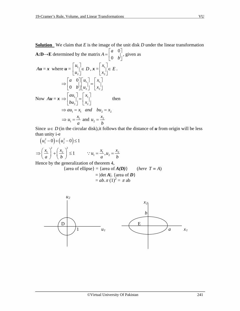
19-Cramer’s Rule, Volume, and Linear Transformations VU
©Virtual University Of Pakistan 241
Solution We claim that E is the image of the unit disk D under the linear transformation
A:D→E determined by the matrix0
0a
Ab
=
, given as
Au = x where u = 1
2
uD
u
∈
, x = 1
2
xE
x
∈
.
Now Au = x
1 1
2 2
1 1
22
1 1 2 2
00
u xau xb
au xxbu
au x and bu x
⇒ =
⇒ =
⇒ = =
then
⇒ 11
xua
= and 22
xub
=
Since u D∈ (in the circular disk),it follows that the distance of u from origin will be less than unity i-e ( ) ( )2 2
1 2
2 21 2 1 2
1 2
0 0 1
1 ,
u u
x x x xu ua b a b
− + − ≤
⇒ + ≤ = =
Hence by the generalization of theorem 4, {area of ellipse} = {area of A(D)} ( )here T A≡ = |det A|. {area of D} = ab.π (1)2 = π ab
u2 x2
b D E 1 u1 a x1

19-Cramer’s Rule, Volume, and Linear Transformations VU
©Virtual University Of Pakistan 242
Example 8 Let S be the parallelogram determined by the vectors 1
13
b =
and 2
51
b =
,
and let 1 10 2
A−
=
. Compute the area of image of S under the mapping x Ax→ .
Solution The area of S is 1 5
det 143 1
=
, and det A = 2. By theorem 4, the area of
image of S under the mapping x Ax→ is |det A|. {area of S} = 2.14 = 28

19-Cramer’s Rule, Volume, and Linear Transformations VU
©Virtual University Of Pakistan 243
Exercises Use Cramer’s Rule to compute the solutions of the systems in exercises 1 and 2.
1. 1 2
1 3
2 3
2x + x =7-3x + x = -8
x + 2x = -3 2.
1 2 3
1 3
1 2 3
2x + x + x = 4-x + 2x = 23x + x +3x = -2
In exercises 3-6, determine the values of the parameter s for which the system has a unique solution, and describe the solution.
3. 1 2
1 2
6sx +4x = 59x +2sx = -2
4. 1 2
1 2
3sx - 5x = 39x +5sx = 2
5. 1 2
1 2
sx - 2sx = -13x +6sx = 4
6. 1 2
1 2
2sx + x = 13sx +6sx = 2
In exercises 7 and 8, compute the adjoint of the given matrix, and then find the inverse of the matrix.
7. 3 5 41 0 12 1 1
8. 3 0 0-1 1 0-2 3 2
In exercises 9 and 10, find the area of the parallelogram whose vertices are listed. 9. (0, 0), (5, 2), (6, 4), (11, 6) 10. (-1, 0), (0, 5), (1, -4), (2, 1) 11. Find the volume of the parallelepiped with one vertex at the origin and adjacent vertices at (1, 0, -2), (1, 2, 4), (7, 1, 0). 12. Find the volume of the parallelepiped with one vertex at the origin and adjacent vertices at (1, 4, 0), (-2, -5, 2), (-1, 2, -1).
13. Let S be the parallelogram determined by the vectors b1 = -23
and b2 = -25
, and
let A = 6 -2-3 2
. Compute the area of the image of S under the mapping →x Ax .

19-Cramer’s Rule, Volume, and Linear Transformations VU
©Virtual University Of Pakistan 244
14. Let S be the parallelogram determined by the vectors b1 = 4-7
and b2 = 01
, and
let A = 7 21 1
. Compute the area of the image of S under the mapping →x Ax .
15. Let T: R3→ R3 be the linear transformation determined by the matrix
0 00 00 0
ab
c
=
A , where a, b, c are positive numbers. Let S be the unit ball, whose
bounding surface has the equation 2 2 21 2 3x x x 1+ + = .
a. Show that T (S) is bounded by the ellipsoid with the equation 22 2
31 22 2 2
xx x 1a b c
+ + = .
b. Use the fact that the volume of the unit ball is 4π / 3 to determine the volume of the region bounded by the ellipsoid in part (a).

20-Vector Spaces and Subspaces VU
©Virtual University Of Pakistan 245
Lecture 20
Vector Spaces and Subspaces
Case Example The space shuttle's control systems are absolutely critical for flight. Because the shuttle is an unstable airframe, it requires constant computer monitoring during atmospheric flight. The flight control system sends a stream of commands to aerodynamic control surfaces. Mathematically, the input and output signals to an engineering system are functions. It is important in applications that these functions can be added, and multiplied by scalars. These two operations on functions have algebraic properties that are completely analogous to the operation of adding vectors in Rn and multiplying a vector by a scalar, as we shall see in the lectures 20 and 27. For this reason, the set of all possible inputs (functions) is called a vector space. The mathematical foundation for systems engineering rests on vector spaces of functions, and we need to extend the theory of vectors in Rn to include such functions. Later on, we will see how other vector spaces arise in engineering, physics, and statistics. Definition Let V be an arbitrary nonempty set of objects on which two operations are defined, addition and multiplication by scalars (numbers). If the following axioms are satisfied by all objects u, v, w in V and all scalars k and l, then we call V a vector space. Axioms of Vector Space 1. Closure Property For any two vectors u & v ∈V, implies u + v ∈V 2. Commutative Property For any two vectors u & v ∈V, implies u + v = v + u 3. Associative Property For any three vectors u, v, w ∈V, u + (v + w) = (u + v) + w 4. Additive Identity For any vector u ∈V, there exist a zero vector 0 such that
0 + u = u + 0 = u
5. Additive Inverse For each vector u ∈V, there exist a vector –u in V such that -u + u = 0 = u + (-u)
6. Scalar Multiplication For any scalar k and a vector u ∈V implies k u ∈V 7. Distributive Law For any scalar k if u & v ∈V, then k (u + v) = k u + k v 8. For scalars m, n and for any vector u ∈V, (m + n) u = m u + n u 9. For scalars m, n and for any vector u ∈V, m (n u) = (m n) u = n (m u)

20-Vector Spaces and Subspaces VU
©Virtual University Of Pakistan 246
10. For any vector u ∈V, 1u = u where 1 is the multiplicative identity of real numbers. Examples of vector spaces The following examples will specify a non empty set V and two operations: addition and scalar multiplication; then we shall verify that the ten vector space axioms are satisfied. Example 1 Show that the set of all ordered n-tuple Rn is a vector space under the standard operations of addition and scalar multiplication. Solution (i) Closure Property: Suppose that u = (u1, u2, …, un) and v = (v1, v2, …, vn) ∈ Rn
Then by definition, u + v = (u1, u2, …, un) + (v1, v2, …, vn) = (u1 + v1, u2 + v2, …, un + vn)∈ Rn (By closure property) Therefore, Rn
is closed under addition. (ii) Commutative Property Suppose that u = (u1, u2, …, un) and v = (v1, v2, …, vn) ∈ Rn
Now u + v = (u1, u2, …, un) + (v1, v2, …, vn) = (u1 + v1, u2 + v2, …, un + vn) (By closure property) = (v1 + u1, v2 + u2, …, vn + un) (By commutative law of real numbers) = (v1, v2, …, vn) + (u1, u2, …, un) (By closure property) = v + u Therefore, Rn is commutative under addition. (iii) Associative Property Suppose that u = (u1, u2, …, un), v = (v1, v2, …, vn) and w = (w1, w2, …, wn)∈Rn Now (u + v) + w = [(u1, u2, …, un) + (v1, v2, …, vn)] + (w1, w2, …, wn) = (u1 + v1, u2 + v2, …, un + vn) + (w1, w2, …, wn) (By closure property) = ((u1 + v1) + w1, (u2 + v2) + w2, …, (un + vn) + wn)) (By closure property) = (u1 + (v1 + w1), u2 + (v2 + w2), …, un + (vn + wn)) (By associative law of real numbers) = (u1, u2, …, un) + (v1 + w1, v2 + w2, …, vn + wn) (By closure property)

20-Vector Spaces and Subspaces VU
©Virtual University Of Pakistan 247
= (u1, u2, …, un) + [(v1, v2, …, vn) + (w1, w2, …, wn)] (By closure property) = u + (v + w) Hence Rn is associative under addition. (iv) Additive Identity Suppose u = (u1, u2, …, un) ∈ Rn. There exists 0 = (0, 0, …, 0) ∈ Rn such that 0 + u = (0, 0, …, 0) + (u1, u2, …, un) = (0 + u1, 0 + u2, …, 0 + un) (By closure property) = (u1, u2, …, un) = u (Existence of identity of real numbers) Similarly, u + 0 = u Hence 0 = (0, 0, …, 0) is the additive identity for Rn. (v) Additive Inverse Suppose u = (u1, u2, …, un) ∈ Rn. There exists -u = (-u1, -u2, …, -un)∈Rn
Such that u + (-u) = (u1, u2, …, un) + (-u1, -u2, …, -un) = (u1 + (-u1), u2 + (-u2), …, un + (-un)) (By closure property) = (0, 0, …, 0) = 0 Similarly, (-u) + u = 0 Hence the inverse of each element of Rn exists in Rn. (vi) Scalar Multiplication If k is any scalar and u = (u1, u2, …, un) ∈ Rn. Then by definition, k u = k (u1, u2, …, un) = (k u1, k u2, …, k un) ∈ Rn
(By closure property) (vii) Distributive Law Suppose k is any scalar and u = (u1, u2, …, un), v = (v1, v2, …, vn) ∈ Rn
Now k (u + v) = k [(u1, u2, …, un) + (v1, v2, …, vn)]

20-Vector Spaces and Subspaces VU
©Virtual University Of Pakistan 248
= k (u1 + v1, u2 + v2, …, un + vn) (By closure property) = (k (u1 + v1), k (u2 + v2), …, k (un + vn)) (By scalar multiplication) = (k u1 + k v1, k u2 + k v2, …, k un + k vn) (By Distributive Law) = (k u1, k u2, …, k un) + (k v1, k v2, …, k vn) (By closure property) = k (u1, u2, …, un) + k (v1, v2, …, vn) (By scalar multiplication) = k u + k v (viii) Suppose k and l be any scalars and u = (u1, u2, …, un) ∈ Rn
Then (k + l) u = (k + l) (u1, u2, …, un) = ((k + l)u1, (k + l)u2, …, (k + l)un) (By scalar multiplication) = (k u1 + l u1, k u2 + l u2, …, k un + l un) (By Distributive Law) = (k u1, k u2, …, k un) + (l u1, l u2, …, l un) (By closure property) = k (u1, u2, …, un) + l (u1, u2, …, un) (By scalar multiplication) = k u + l u (ix) Suppose k and l be any scalars and u = (u1, u2, …, un) ∈ Rn
Then k (l u) = k [l (u1, u2, …, un)] = k (l u1, l u2, …, l un) (By scalar multiplication) = (k (l u1), k (l u2), …, k (l un)) (By scalar multiplication) = ((k l)u1, (k l)u2, …, (k l)un) (By associative law) = (k l) (u1, u2, …, un) (By scalar multiplication) = (k l) u (x) Suppose u = (u1, u2, …, un) ∈ Rn Then 1 u = 1 (u1, u2, …, un) = (1u1, 1u2, …, 1un) (By scalar multiplication)

20-Vector Spaces and Subspaces VU
©Virtual University Of Pakistan 249
= (u1, u2, …, un) = u (Existence of identity in scalrs) Hence, Rn is the real vector space with the standard operations of addition and scalar multiplication. Note The three most important special cases of Rn are R (the real numbers), R2 (the vectors in the plane), and R3 (the vectors in 3-space). Example 2 Show that the set V of all 2x2 matrices with real entries is a vector space if vector addition is defined to be matrix addition and vector scalar multiplication is defined to be matrix scalar multiplication.
Solution Suppose that and11 12 11 12 11 12
21 22 21 22 21 22
u u v v w w= , = =
u u v v w w
∈
u v w V
and k and l be two any scalars. (i) Closure property To prove axiom (i), we must show that u + v is an object in V: that is , we must show that u + v is a 2x2 matrix. But this is clear from the definition of matrix
addition, since 11 12 11 12 11 11 12 12
21 22 21 22 21 21 22 22
u u v v u +v u +v+ = + =
u u v v u +v u +v
u v
(By closure property)
(ii) Commutative property Now it is very easy to verify the Axiom (ii)
11 12 11 12 11 11 12 12
21 22 21 22 21 21 22 22
u u v v u +v u +v+ = + =
u u v v u +v u +v
u v (By closure property)
11 11 12 12
21 21 22 22
v +u v +u=
v +u v +u
(Commutative property of real numbers)
11 12 11 12
21 22 21 22
v v u u= + = +
v v u u
v u
(iii) Associative property 11 12 11 12 11 12
21 22 21 22 21 22
u u v v w w( + ) + = + +
u u v v w w
u v w
11 11 12 12 11 12
21 21 22 22 21 22
u +v u +v w w= +
u +v u +v w w
(By closure property)
11 11 11 12 12 12
21 21 21 22 22 22
(u +v )+ w (u +v )+ w=
(u +v )+ w (u +v )+ w
11 11 11 12 12 12
21 21 21 22 22 22
u +(v + w ) u +(v + w )=
u +(v + w ) u +(v + w )
(By associative property of real numbers)

20-Vector Spaces and Subspaces VU
©Virtual University Of Pakistan 250
11 12 11 11 12 12
21 22 21 21 22 22
u u v + w v + w= +
u u v + w v + w
11 12 11 12 11 12
21 22 21 22 21 22
u u v v w w= + + = + ( + )
u u v v w w
u v w
Therefore, V is associative under ‘+’. (iv) Additive Identity Now to prove the axiom (iv), we must find an object 0 in V such
that 0 + v = v + 0 = v for all u in V. This can be done by defining 00 0
=0 0
.
11 12
21 22
u u0 0+ = +
u u0 0
u0 11 12 11 12
21 22 21 22
0+u 0+u u u= = =
0+u 0+u u u
u
and similarly u + 0 = u. (v) Additive Inverse Now to prove the axiom (v) we must show that each object u in V has a negative –u such that u + (-u) = 0 = (-u) + 0. Defining the negative of u to be
11 12
21 22
-u -u- =
-u -u
u .
( ) ( )( ) ( )
11 11 12 1211 12 11 12
21 21 22 2221 22 21 22
u + -u u + -uu u -u -u 0 0+(- )= + = = =
u + -u u + -uu u -u -u 0 0
u u 0
Similarly, (-u) + u = 0 (vi) Scalar Multiplication Axiom (vi) also holds because for any real number k we have
11 12 11 12
21 22 21 22
u u ku kuk = k =
u u ku ku
u (By closure property)
so that k u is a 2x2 matrix and consequently is an object in V. (vii) Distributive Law
11 12 11 12
21 22 21 22
u u v vk ( + )= k +
u u v v
u v
20-Vector Spaces and Subspaces VU
©Virtual University Of Pakistan 251
11 11 12 12 11 11 12 12
21 21 22 22 21 21 22 22
u +v u +v k(u +v ) k(u +v )= k =
u +v u +v k(u +v ) k(u +v )
11 11 12 12 11 12 11 12
21 21 22 22 21 22 21 22
11 12 11 12
21 22 21 22
ku + kv ku + kv ku ku kv kv= = +
ku + kv ku + kv ku ku kv kv
u u v v= k + k = k + k
u u v v
u v
(viii) 11 12 11 12
21 22 21 22
u u (k + l)u (k + l)u(k + l) = (k + l) =
u u (k + l)u (k + l)u
u
11 11 12 12
21 21 22 22
ku + lu ku + lu=
ku + lu ku + lu
11 12 11 12
21 22 21 22
ku ku lu lu= +
ku ku lu lu
11 12 11 12
21 22 21 22
u u u u= k + l = k + l
u u u u
u u
(ix) 11 12 11 12
21 22 21 22
u u lu luk(l ) = k l = k
u u lu lu
u
11 12 11 12
21 22 21 22
k(lu ) k(lu ) (kl)u (kl)u= =
k(lu ) k(lu ) (kl)u (kl)u
11 12
21 22
u u= (kl)
u u
= (kl)u
(x) Finally axiom (x) is a simple computation
11 12 11 12 11 12
21 22 21 22 21 22
u u 1u 1u u u1 = 1 = = =
u u 1u 1u u u
u u
Hence the set of all 2x2 matrices with real entries is vector space under matrix addition and matrix scalar multiplication. Note Example 2 is a special case of a more general class of vector spaces. The arguments in that example can be adapted to show that a set V of all m×n matrices with real entries, together with the operations of matrix addition and scalar multiplication, is a vector space.
20-Vector Spaces and Subspaces VU
©Virtual University Of Pakistan 252
Example 3 Let V be the set of all real-valued functions defined on the entire real line( , )−∞ ∞ . If f, g∈V, then f + g is a function defined by (f +g) (x) = f (x) + g (x), for all x∈R. The product of a scalar a∈R and a function f in V is defined by (a f) (x) = a f (x), for all x∈R. Solution (i) Closure Property If f, g∈V, then by definition (f +g) (x) = f (x) + g (x) ∈V. Therefore, V is closed under addition. (ii) Commutative Property If f and g are in V, then for all x∈R (f + g) (x) = f (x) + g (x) (By definition) = g (x) + f (x) (By commutative property) = (g + f) (x) (By definition) So that f + g = g + f (iii) Associative Property If f, g and h are in V, then for all x∈R ((f + g) + h) (x) = (f + g) (x) + h (x) (By definition) = (f (x) + g (x)) + h (x) (By definition) = f (x) + (g (x) + h (x)) (By associative property) = f (x) + (g + h) (x) (By definition) = (f + (g + h)) (x) And so (f + g) + h = f + (g + h) (iv) Additive Identity The additive identity of V is the zero function defined by 0 (x) = 0, for all x∈R because (0 + f) (x) = 0 (x) + f (x) (By definition) = 0 + f (x) = f (x) (Existence of identity) i.e. 0 + f = f. Similarly, f + 0 = f. (v) Additive Inverse The additive inverse of a function f in V is (-1) f = -f∈V because (f + (-f)) (x) = f (x) + (-f) (x) (By definition) = f (x) – f (x) (By definition) = 0 (Existence of inverse)

20-Vector Spaces and Subspaces VU
©Virtual University Of Pakistan 253
i.e. f + (-f) = 0. Similarly, (-f) + f = 0. (vi) Scalar Multiplication If f is in V and a is in R, then by definition (a f) (x) = a f (x) ∈V. (vii) Distributive Law If f, g are in V and a∈R, then (a (f + g)) (x) = a (f + g) (x) = a (f (x) + g (x)) = a f (x) + a g (x) = (a f) (x) + (a g) (x) = (a f + a g) (x) and, therefore, a (f + g) = a f + a g (viii) Let a, b in R and f∈V, then ((a + b) f) (x) = (a + b) f (x) = a f (x) + b f (x) = (a f) (x) + (b f) (x) = (a f + b f) (x) Thus (a + b) f = a f + b f (ix) a (b f) (x) = a (b f (x)) = (a b) f (x) showing that a (b f) = (a b) f (x) (1.f) (x) = 1 f (x) = f (x) (Existence of identity) And so 1.f = f Hence V is a real vector space. Example 4 If 0 1 2 n( ) = a + a + a + . . . + a2 np x x x x
and 0 1 2 n ( ) = b + b + b + . . . + b2 nq x x x x We define
0 1 2 n 0 1 2 n( )+ ( ) = (a + a + a + . . . + a )+(b + b + b + . . . + b )2 n 2 np x q x x x x x x x
0 0 1 1 2 2 n n= (a +b )+(a +b ) +(a +b ) +...+(a +b )2 nx x x and for any scalar k,
0 1 2 nk ( ) = k(a + a + a + . . . + a )2 np x x x x 0 1 2 n= ka + ka + ka + . . . + k a2 nx x x Clearly the given polynomial is a vector space under the addition and scalar multiplication. Example 5 (The Zero Vector Space) Let V consists of a single object, which we define by 0 and 0 + 0 = 0 and k 0 = 0 for all scalars k. It is easy to check that all the vector space axioms are satisfied. We call V={0} as the zero vector space.

20-Vector Spaces and Subspaces VU
©Virtual University Of Pakistan 254
Example 6 (Every plane through the origin is a vector space) Let V be any plane through the origin in R3
. We shall show that the points in V form a vector space under a standard addition and scalar multiplication operations for vectors in R3. From example1, we know that R3 itself is a vector space under these operations. Thus, Axioms 2, 3, 7, 8, 9 and 10 hold for all points in R3 and consequently for all points in the plane V. We therefore need only show that Axioms 1, 4, 5 and 6 are satisfied. Since the plane is passing through the origin, it has an equation of the form
a x + b y + c z = 0 (1)
Thus, if u = (u1, u2, u3) and v = (v1, v2, v3) are points in V, then
a u1 + b u2 + c u3 = 0 and a v1 + b v2 + c v3 = 0.
Adding these equations gives a (u1 + v1) + b (u2 + v2) + c (u3 + v3) = 0 This equality tell us that the coordinates of the point u + v = (u1 + v1, u2 + v2, u3 + v3) satisfies (1); thus, u + v lies in plane V. This proves that the Axiom 1 is satisfied. There exists 0 = (0, 0, 0) such that a (0) +b (0) + c (0) = 0. Therefore, Axiom 4 is satisfied. Multiplying a u1 + b u2 + c u3 = 0 through by k gives a (ku1) + b (ku2) + c (ku3) = 0 Thus, (ku1, k u2, k u3) = k (u1, u2, u3) = k u∈V. Hence, Axiom 6 is satisfied. We shall prove the axiom 5 is satisfied. Multiplying a u1 + b u2 + c u3 = 0 through by -1 gives a (-1u1) + b (-1u2) + c (-1u3) = 0 Thus, (-u1, - u2, - u3) = - (u1, u2, u3) = -u∈V. This establishes Axiom 5. Example 7 (A set that is not a vector space) Let V=R2 and define addition and scalar multiplication operation as follows. If
1 2 1 2= (u ,u )and = (v ,v )u v then define
1 1 2 2+ = (u +v ,u +v )u v and if k is any real number then define 1k = (ku ,0)u . For any vector u ∈V, 1u =1(u1, u2) = (1 u1, 0) = (u1, 0) ≠ u where 1 is the multiplicative identity of real numbers. Therefore, the axiom 10 is not satisfied. Hence, V=R2 is not a vector space.

20-Vector Spaces and Subspaces VU
©Virtual University Of Pakistan 255
Theorem 1 Let V be a vector space, u a vector in V, and k is a scalar, then (i) 0u = 0 (ii) k0 = 0 (iii) (-1) u = -u (iv) If k u = 0 then k = 0 or u = 0 Definition A subset W of a vector space V is called a subspace of V if W itself a vector space under the addition and scalar multiplication defined on V. Note If W is a part of a larger set V that is already known to be a vector space, then certain axioms need not be verified for W because they are “inherited” from V. For example, there is no need to check that u + v = v + u (Axiom 2) for W because this holds for all vectors in V and consequently for all vectors in W. Other Axioms are inherited by W from V are 3, 7, 8, 9, and 10. Thus, to show that a set W is a subspace of a vector space V, we need only verify Axioms 1, 4, 5 and 6. The following theorem shows that even Axioms 4 and 5 can be omitted. Theorem 2 If W is a set of one or more vectors from a vector space V, then W is subspace of V if and only if the following conditions hold.
(a) If u and v are vectors in W, then u + v is in W (b) If k is any scalar and u is any vector in W, then k u is in W.
Proof If W is a subspace of V, then all the vector space axioms are satisfied; in particular, Axioms 1 and 6 hold. But these are precisely conditions (a) and (b). Conversely, assume conditions (a) and (b) hold. Since these conditions are vector space Axioms 1 and 6, we need only show that W satisfies the remaining 8 axioms. The vectors in W automatically satisfy axioms 2, 3, 7, 8, 9, and 10 since they are satisfied by all vectors in V. Therefore, to complete the proof, we need only to verify that vectors in W satisfy axioms 4 and 5. Let u be any vector in W. By condition (b), k u is in W for every scalar k. Setting k = 0, it follows from theorem 1 that 0 u = 0 is in W, and setting k = - 1, it follows that (-1) u = -u is in W. Remark (1) The theorem states that W is a subspace of V if and only if W is closed under addition and closed under scalar multiplication. (2) Every vector space has at least two subspaces, itself and the subspace {0} consisting only of the zero vector. Thus the subspace {0} is called the zero subspace. Example 8 Let W be the subset of R3 consisting of the all the vectors of the form (a, b, 0), where a and b are real numbers. To check if W is subspace of R3, we first see that axiom 1 and 6 of a vector space holds.

20-Vector Spaces and Subspaces VU
©Virtual University Of Pakistan 256
Let 1 1 2 2= (a ,b ,0) and = (a ,b ,0)u v be vectors in W then
1 1 2 2 1 2 1 2+ = (a ,b ,0) +(a ,b ,0)= (a + a ,b +b ,0)u v is in W. Since the third component is zero. Also c is scalar, and then 1 1 1 1c = c(a ,b ,0)= (ca ,cb ,0)u is in W. Therefore the Ist and 6th axioms of the vector space holds. We can also verify the other axioms of vector space. Hence W is a subspace. Example 9 Consider the set W consisting of all 2x3 matrices of the form
00a b
c d
, Where a, b, c and d are arbitrary real numbers. Show that the W is a
subspace M2x3.
Solution Consider 0 0
0 01 1 2 2
1 1 2 2
a b a b= , =
c d c d
u v in W
Then 0 0 0
0 0 01 1 2 2 1 2 1 2
1 1 2 2 1 2 1 2
a b a b a + a b +b+ = + =
c d c d c +c d + d
u v is in W.
So that the (a) part of the theorem is satisfied. Also k is a scalar, and then 0
01 1
1 1
ka kbk =
kc kd
u is in W. So the (b) part of the above theorem is also satisfied.
Hence W is a subspace of M2x3. Note Let V is a vector space then every subset of V is not necessary a subspace of V. For example, let V =R2 then any line in R2 not passing through origin is not a subspace of R2. Similarly, a plane in R3 not passing through the origin is not a subspace of R3. Example 10 Let W be the subset of R3 consisting of all vectors of the form (a, b, 1), where a, b are any real numbers. To check whether property (a) and (b) of the above theorem holds. Let 1 1 2 2= (a ,b ,1)and = (a ,b ,1)u v be vectors in W. Then 1 1 2 2 1 2 1 2+ = (a ,b ,1)+(a ,b ,1)= (a + a ,b +b ,1+1)u v which is not in W because the third component 2 is not 1. As the Ist property does not hold therefore, the given set of vectors is not a vector space. Example 11 Which of the following are subspaces of R3 (i) All vectors of the form (a, 0, 0) (ii) All vectors of the form (a, 1, 1) (iii) All vectors of the form (a, b, c), where b = a + c (iv) All vectors of the form (a, b, c), where b = a + c +1 Solution Let W is the set of all vectors of the form (a, 0, 0). (i) Suppose u = (u1, 0, 0) and v = (v1, 0, 0) are in W. Then u + v = (u1, 0, 0) + (v1, 0, 0) = (u1 + v1, 0, 0) which is of the form (a, 0, 0).

20-Vector Spaces and Subspaces VU
©Virtual University Of Pakistan 257
Therefore, u + v∈W If k is any scalar and u = (u1, 0, 0) is any vector in W, then k u = k (u1, 0, 0) = (k u1, 0, 0) which is of the form (a, 0, 0). Therefore, k u∈W. Hence W is the subspace of R3. (ii) Let W is the set of all vectors of the form (a, 1, 1). Suppose u = (u1, 1, 1) and v = (v1, 1, 1) are in W. Then u + v = (u1, 1, 1) + (v1, 1, 1) = (u1 + v1, 2, 2) which is not of the form (a, 1, 1). Therefore, u + v∉W. Hence W is not the subspace of R3. (iii) Suppose W is the set of all vectors of the form (a, b, c), where b = a + c Suppose u = (u1, u1 + u3, u3) and v = (v1, v1 + v3, v3) are in W. Then u + v = (u1, u1 + u3, u3) + (v1, v1 + v3, v3) = (u1 + v1, u1 + u3 + v1 + v3, u3 + v3) = (u1 + v1, (u1 + v1) + (u3 + v3), u3 + v3), which is of the form (a, a + c, c). Therefore, u + v∈W If k is any scalar and u = (u1, u1 + u3, u3) is any vector in W, then k u = k (u1, u1 + u3, u3) = (k u1, k (u1 + u3), k u3) (By definition) = (k u1, k u1 + k u3, k u3) (By Distributive Law) Which is of the form (a, a + c, c). Therefore, k u∈W. Hence W is the subspace of R3. (iv) Let W is the set of all vectors of the form (a, b, c), where b = a + c +1 Suppose u = (u1, u1 + u3 + 1, u3) and v = (v1, v1 + v3 + 1, v3) are in W. Then u + v = (u1, u1 + u3 + 1, u3) + (v1, v1 + v3 + 1, v3) = (u1 + v1, u1 + u3 + 1 + v1 + v3 + 1, u3 + v3) = (u1 + v1, (u1 + v1) + (u3 + v3) + 2, u3 + v3) Which is not of the form (a, a + c + 1, c). Therefore, u + v∉W. Hence W is not the subspace of R3. Example 12 Determine which of the following are subspaces of P3. (i) All polynomials a0 + a1 x + a2 x2 + a3 x3 for which a0 = 0 (ii) All polynomials a0 + a1 x + a2 x2 + a3 x3 for which a0 + a1 + a2 + a3 = 0 (iii) All polynomials a0 + a1 x + a2 x2 + a3 x3 for which a0, a1, a2, and a3 are integers (iv) All polynomials of the form a0 + a1 x, where a0 and a1 are real numbers.

20-Vector Spaces and Subspaces VU
©Virtual University Of Pakistan 258
Solution (i) Let W is the set of all polynomials a0 + a1 x + a2 x2 + a3 x3 for which a0 = 0. Suppose that u = c0 + c1 x + c2 x2 + c3 x3 (where c0 = 0) and v = b0 + b1 x + b2 x2 + b3 x3 (where b0 = 0) are in W. Then u + v = (c0 + c1x + c2x2 + c3x3) + (b0 + b1x + b2x2 + b3x3) = (c0 + b0) + (c1 + b1)x + (c2 + b2)x2 + (c3 + b3) x3, where c0 + b0 = 0. Therefore, u + v ∈W If k is any scalar and u = c0 + c1 x + c2 x2 + c3 x3 (where c0 = 0) is any vector in W. Then k u = k (c0 + c1x + c2x2 + c3x3) = (kc0) + (kc1) x + (kc2) x2 + (kc3) x3 where k c0 = 0. Therefore, k u∈W. Hence W is the subspace of P3. (ii) Let W is the set of all polynomials a0 + a1x + a2x2 + a3x3 for which a0+a1+a2+a3 = 0. Suppose that u = c0 + c1 x + c2 x2 + c3 x3 (where c0 + c1 + c2 + c3 = 0) and v = b0 + b1 x + b2 x2 + b3 x3 (where b0 + b1 + b2 + b3 = 0) are in W. Now u + v = (c0 + c1 x + c2 x2 + c3 x3) + (b0 + b1 x + b2 x2 + b3 x3) = (c0 + b0) + (c1 + b1) x + (c2 + b2) x2 + (c3 + b3) x3 Where (c0+b0) + (c1+b1) + (c2+b2) + (c3+b3) = (c0+c1+c2+c3) + (b0+b1+b2+b3) = 0 + 0 = 0. Therefore, u + v ∈W If k is any scalar and u = c0 + c1 x + c2 x2 + c3 x3 (where c0 + c1 + c2 + c3 = 0) is any vector in W. Then k u = k (c0 + c1x + c2x2 + c3x3) = (kc0) + (kc1) x + (kc2) x2 + (kc3) x3 Where (k c0) + (k c1) + (k c2) + (k c3) = k(c0 + c1 + c2 + c3) = k.0 = 0 Therefore, k u∈W. Hence W is the subspace of P3. (iii) Let W is the set of all polynomials a0 + a1 x + a2 x2 + a3 x3 for which a0, a1, a2, and a3 are integers. Suppose that the vectors u = c0 + c1 x + c2 x2 + c3 x3 (where c0, c1, c2, and c3 are integers) and v = b0 + b1 x + b2 x2 + b3 x3 (where b0, b1, b2, and b3 are integers) are in W. Now u + v = (c0 + c1 x + c2 x2 + c3 x3) + (b0 + b1 x + b2 x2 + b3 x3) = (c0 + b0) + (c1 + b1) x + (c2 + b2) x2 + (c3 + b3) x3, where (c0 + b0), (c1 + b1), (c2 + b2), and (c3 + b3) are integers (integers are closed under addition). Therefore, u + v ∈W If k is any scalar and u = c0 + c1 x + c2 x2 + c3 x3 (where c0, c1, c2, and c3 are integers) is any vector in W. Then k u = k (c0 + c1x + c2x2 + c3x3 = (kc0) + (kc1) x + (kc2) x2 + (kc3) x3, where (k c0), (k c1), (k c2), and (k c3) are not integers (product of real number and integer). Therefore, k u∉W. Hence, W is not the subspace of P3.

20-Vector Spaces and Subspaces VU
©Virtual University Of Pakistan 259
(iv) Let W is the set of all polynomials of the form a0 + a1 x, where a0 and a1 are real numbers. Suppose that u = c0 + c1 x (where c0 and c1 are real numbers) and v = b0 + b1 x (where b0 and b1 are real numbers) are in W. Then u + v = (c0 + c1 x) + (b0 + b1 x) = (c0 + b0) + (c1 + b1) x Where (c0 + b0) and (c1 + b1) are real numbers. Therefore, u + v ∈W If k is any scalar and u = c0 + c1 x (where c0 and c1 are real numbers) is any vector in W. Then k u = k (c0 + c1 x) = (k c0) + (k c1) x Where (k c0) and (k c1) are real numbers. Therefore, k u∈W. Hence W is the subspace of P3. Example 13 Determine which of the following are subspaces of M22.
(i) All matrices a bc d
where a + b +c + d = 0
(ii) All 2 x 2 matrices A such that det (A) = 0
(iii) All the matrices of the form 0a b
c
Solution Let W is the set of all matrices a bc d
where a + b +c + d = 0.
(i) Suppose u = e fg h
(where e + f + g + h = 0) and v = l mn p
(Where l + m + n + p = 0) are in W.
Then u + v = e fg h
+ l mn p
= e + l f + mg + n h + p
(By definition)
Where (e + l) + (f + m) + (g + n) + ( h + p) = (e + f + g + h) + (l + m + n + p) = 0 + 0 = 0 Therefore, u + v∈W
If k is any scalar and u = e fg h
(where e + f + g + h = 0) is any vector in W.
Then k u = ke fg h
=ke kfkg kh
(by definition)
Where k e + k f + k g + k h = k (e + f + g + h) = k 0 = 0 Hence, k u∈W. Therefore, W is subspace of M22. (ii) Let W is the set of all 2 x 2 matrices A such that det (A) = 0
Suppose u = e fg h
(Where det (u) = e h – f g = 0) and v = l mn p

20-Vector Spaces and Subspaces VU
©Virtual University Of Pakistan 260
(Where det (v) = l p – m n = 0) are in W.
Then u + v = e fg h
+ l mn p
= e + l f + mg + n h + p
(By definition)
Where det (u + v) = (e + l) (h + p) - (f + m) (g + n) = e h + e p + l h + l p – f g – f n – m g – m n = (e h – f g) + (l p – m n) + e p + l h – f n – m g = e p + l h – f n – m g ≠ 0 Therefore, u + v∉W. Therefore, W is not subspace of M22.
(iii) Let W is the set of all matrices of the form 0a b
c
Suppose u = 0e f
g
and v = 0l m
n
are in W.
Then u + v = 0e f
g
+ 0l m
n
= 0
e + l f + mg + n
(By definition)
Which is of the form0a b
c
. Therefore, u + v∈W
If k is any scalar and u = 0e f
g
is any vector in W.
Then k u = k0e f
g
=0ke kf
kg
(By definition)
Which is of the form0a b
c
. Hence, k u∈W
Therefore, W is subspace of M22. Example 14 Determine which of the following are subspaces of the space (- , )∞ ∞F . (i) All f such that f (x) ≤ 0 for all x (ii) all f such that f (0) = 0 (iii) All f such that f (0) = 2 (iv) all constant functions (v) All f of the form k1 + k2 sin x, where k1 and k2 are real numbers (vi) All everywhere differentiable functions that satisfy + 2 = 0′f f . Solution (i) Let W is the set of all f such that f (x) ≤ 0 for all x. Suppose g and h are the vectors in W. Then g (x) ≤ 0 for all x and h (x) ≤ 0 for all x. Now (g + h) (x) = g (x) + h (x) ≤ 0. Therefore, + ∈g h W If k is any scalar and g is any vector in W. Then g (x) ≤ 0 for all x Now (k g) (x) = k g (x), which is greater than 0 for negative real values of k.
k k < 0∴ ∉ ∀g W . Hence W is not the subspace of (- ),∞ ∞F .

20-Vector Spaces and Subspaces VU
©Virtual University Of Pakistan 261
(ii) Let W is the set of all f such that f (0) = 0. Suppose g and h are the vectors in W. Then g (0) = 0 and h (0) = 0 Now (g + h) (0) = g (0) + h (0) = 0 + 0 = 0. Therefore, + ∈g h W If k is any scalar and g is any vector in W. Then g (0) = 0 Now (k g) (0) = k g (0) = k 0 = 0. k∴ ∈g W . Hence W is the subspace of (- , )∞ ∞F . (iii) Let W is the set of all f such that f (0) = 2 Suppose g and h are the vectors in W. Then g (0) = 2 and h (0) = 2 Now (g + h) (0) = g (0) + h (0) = 2 + 2 ≠ 2 k∴ ∉g W . Hence W is not the subspace of
(- , )∞ ∞F . (iv) Let W is the set of all constant functions. Suppose g and h are the vectors in W. Then g (x) = a and h (x) = b, where a and b are constants. Now (g + h) (x) = g (x) + h (x) = a + b, which is constant. Therefore, + ∈g h W If k is any scalar and g is any vector in W. Then g (x) = a, where a is any constant. Now (k g) (x) = k g (x) = k a, which is a constant. k∴ ∈g W . Hence W is the subspace of (- , )∞ ∞F . (v) Let W is the set of all f of the form k1 + k2 sin x, where k1 and k2 are real numbers Suppose g and h are the vectors in W. Then g (x) = m1+m2sin x and h (x) = n1+n2 sin x, where m1, m2, n1and n2 are real numbers. Now (g + h) (x) = g (x) + h (x) = [m1+m2sin x]+[n1+n2sin x] = (m1+n1)+(m2+n2) sin x Which is of the form k1 + k2 sin x. Therefore, + ∈g h W If k is any scalar and g is any vector in W. Then g (x) = m1 + m2 sin x, where m1 and m2 are any real numbers. Now (k g) (x) = k g (x) = k [m1 + m2 sin x] = (k m1) + (k m2) sin x Which is of the form k1 + k2 sin x. k∴ ∈g W . Hence W is the subspace of (- , )∞ ∞F . (vi) Let W is the set of all everywhere differentiable functions that satisfy + 2 =′f f 0 . Suppose g and h are the vectors in W. Then + 2 =′g g 0 and + 2 =′h h 0 Now ( + ) + 2( + ) = + + 2( + )′ ′ ′g h g h g h g h = ( + 2 )+ ( + 2 )′ ′g g h h = 0 + 0 = 0 Therefore, + ∈g h W If k is any scalar and g is any vector in W. Then + 2 =′g g 0 Now (k ) + 2(k ) = k + 2k′ ′g g g g = k( + 2 ) = k. =′g g 0 0
k∴ ∈g W . Hence W is the subspace of (- , )∞ ∞F .

20-Vector Spaces and Subspaces VU
©Virtual University Of Pakistan 262
Remark Let n be a non-negative integer, and let nP be the set of real valued function of
the form 0 1 2 n( )= a + a + a +...+ a2 np x x x x where 0 1 2, , ,..., na a a a are real numbers, then nP is a subspace (- , )∞ ∞F . Example 15 Show that the invertible n x n matrices do not form a subspace of M n x n. Solution Let W is the set of invertible matrices in M n x n. This set fails to be a subspace on both counts- it is closed under neither scalar multiplication nor addition.
For example consider invertible matrices 1 2 -1 2
in2 5 -2 5
= , =
n x nW V M .
The matrix 0.U is a 2x2 zero matrix, hence is not invertible; and the matrix U + V has a column of zeros, hence is not invertible. Theorem If Ax = 0 is a homogeneous linear system of m equations in n unknowns, then the set of solution vectors is a subspace of Rn. Example 16 Consider the linear systems
1 -2 3 0 1 -2 3 02 -4 6 = 0 -3 7 -8 = 03 -6 9 0 -2 4 -6 0
1 -2 3 0 0 0 0 0-3 7 -8 = 0 0 0 0 = 04 1 2 0 0 0 0 0
x x(a) y (b) y
z z
x x(c) y (d) y
z z
Each of the systems has three unknowns, so the solutions form subspaces of R3. Geometrically, this means that each solution space must be a line through origin, a plane through origin, the origin only, or all of R3. Solution (a) The solutions are x = 2s - 3t, y = s, z = t. From which it follows that x = 2y - 3z or x - 2y + 3z = 0. This is the equation of the plane through the origin with n =(1, -2,3) as a normal vector. (b) The solutions are x = -5t, y = - t, z = t, which are parametric equations for the line through the origin parallel to the vector v =(-5, -1,1). (c) The solution is x = 0, y = 0, z = 0 so the solution space is the origin only, that is {0}. (d)The solutions are x = r, y = s, z = t. where r, s and t have arbitrary values, so the solution space is all R3. A Subspace Spanned by a Set: The next example illustrates one of the most common ways of describing a subspace. We know that the term linear combination refers to any

20-Vector Spaces and Subspaces VU
©Virtual University Of Pakistan 263
sum of scalar multiples of vectors, and Span {v1, … , vp} denotes the set of all vectors that can be written as linear combinations of v1, … , vp. Example 17 Given v1 and v2 in a vector space V, let H = Span {v1, v2}. Show that H is a subspace of V. Solution The zero vector is in H, since 0 = 0v1 + 0v2. To show that H is closed under vector addition, take two arbitrary vectors in H, say, u = s1v1 +s2v2 and w = t1v1 + t2v2 By Axioms 2, 3 and 8 for the vector space V. u + w = (s1v1 +s2v2) + (t1v1 + t2v2) = (s1 + t1) v1 + (s2 + t2) v2 So u + w is in H. Furthermore, if c is any scalar, then by Axioms 7 and 9,
cu = c (s1v1 + s2v2) = (cs1) v1 + (cs2)v2
Which shows that cu is in H and H is closed under scalar multiplication. Thus H is a subspace of V. Later on we will prove that every nonzero subspace of R3, other than R3 itself, is either Span {v1, v2} for some linearly independent v1 and v2 or Span {v} for .≠v 0 In the first case the subspace is a plane through the origin and in the second case a line through the origin. (See Figure below) It is helpful to keep these geometric pictures in mind, even for an abstract vector space.
Figure 9 – An example of a subspace
The argument in Example 17 can easily be generalized to prove the following theorem.
0
x2 x1
x3
v2
v1

20-Vector Spaces and Subspaces VU
©Virtual University Of Pakistan 264
Theorem 3 If v1, … , vp are in a vector space V, then Span {v1, …, vp} is a subspace of V. We call Span {v1, … , vp} the subspace spanned (or generated) by {v1,… , vp}. Given any subspace H of V, a spanning (or generating) set for H is a set {v1, …, vp} in H such that H = Span {v1, …, vp}. Proof
The zero vector is in H, since 0 = 0v1 + 0v2+ …+0vn=00
j n
jj
v=
=∑ =0
0
j n
jj
v=
=
∑ =0
To show that H is closed under vector addition, take two arbitrary vectors in H, say,
u = s1v1 +s2v2+…+tnvn=0
i n
i ii
s v=
=∑
and
w = t1v1 + t2v2 …+tnvn=0
k n
k kk
t v=
=∑
By Axioms 2, 3 and 8 for the vector space V.
u + w = 0
i n
i ii
s v=
=∑ +
0
k n
k kk
t v=
=∑ = (s1v1 +s2v2+…+snvn )+( t1v1 + t2v2 …+tnvn)
= (s1 + t1) v1 + (s2 + t2) v2+…+(sn + tn) vn=0( )
p n
p p pp
s t v=
=
+∑
So u + w is in H. Furthermore, if c is any scalar, then by Axioms 7 and 9,
cu = c(s1v1 +s2v2+…+snvn )= (cs1) v1 + (cs2)v2+…+(csn )vn=0
r n
r rr
cs v=
=∑ .
Which shows that cu is in H and H is closed under scalar multiplication. Thus H is a subspace of V. Example 18 Let H be the set of all vectors of the form (a – 3b, b – a, a, b), where a and b are arbitrary scalars. That is, let H = {(a – 3b, b – a, a, b): a and b in R}. Show that H is a subspace of R4. Solution Write the vectors in H as column vectors. Then an arbitrary vector in H has the form
3 1 31 1
1 00 1
a bb a
a bab
− − − − = +
↑ ↑
1 2v v

20-Vector Spaces and Subspaces VU
©Virtual University Of Pakistan 265
This calculation shows that H = Span {v1, v2}, where v1 and v2 are the vectors indicated above. Thus H is a subspace of R4 by Theorem 3. Example18 illustrates a useful technique of expressing a subspace H as the set of linear combinations of some small collection of vectors. If H = Span {v1, …, vp}, we can think of the vectors v1, … , vp in the spanning set as “handles” that allow us to hold on to the subspace H. Calculations with the infinitely many vectors in H are often reduced to operations with the finite number of vectors in the spanning set.

20-Vector Spaces and Subspaces VU
©Virtual University Of Pakistan 266
Exercises In exercises 1-13 a set of objects is given together with operations of addition and scalar multiplication. Determine which sets are vector spaces under the given operations. For those that are not, list all axioms that fail to hold. 1. The set of all triples of real numbers (x, y, z) with the operations
and(x, y,z)+(x , y ,z )= (x+ x , y+ y ,z + z ) k(x, y,z)= (kx, y,z)′ ′ ′ ′ ′ ′ 2. The set of all triples of real numbers (x, y, z) with the operations
and(x, y,z)+(x , y ,z )= (x+ x , y+ y ,z + z ) k(x, y,z)= (0,0,0)′ ′ ′ ′ ′ ′ 3. The set of all pairs of real numbers (x, y) with the operations
and(x, y)+(x , y )= (x+ x , y+ y ) k(x, y)= (2kx,2ky)′ ′ ′ ′ 4. The set of all pairs of real numbers of the form (x, 0) with the standard operations on R2. 5. The set of all pairs of real numbers of the form (x, y), where x≥0, with the standard operations on R2. 6. The set of all n-tuples of real numbers of the form (x, x, …, x) with the standard operations on Rn. 7. The set of all pairs of real numbers (x, y) with the operations. and(x, y)+(x , y )= (x+ x +1, y+ y +1) k(x, y)= (kx,ky)′ ′ ′ ′
8. The set of all 2x2 matrices of the form 1
1a
b
with matrix addition and scalar
multiplication.
9. The set of all 2x2 matrices of the form 0
0a
b
with matrix addition and scalar
multiplication. 10. The set of all pairs of real numbers of the form (1, x) with the operations
(1, ) (1, ) (1, ) and (1, ) (1, )y y y y k y ky′ ′+ = + = 11. The set of polynomials of the form a + bx with the operations and1 1 1 1 1 1( +a )+( +b )= ( + )+(a +b ) k( +a )= (k )+(ka )0 0 0 0 0 0a x b x a b x a x a x 12. The set of all positive real numbers with operations x + y = xy and kx = xk 13. The set of all real numbers (x, y) with operations

20-Vector Spaces and Subspaces VU
©Virtual University Of Pakistan 267
, , , and , ,( x y ) ( x y ) ( xx yy ) k( x y ) ( kx ky )′ ′ ′ ′+ = = 14. Determine which of the following are subspaces of Mnn. (a) all n x n matrices A such that tr (A) = 0 (b) all n x n matrices A such that AT = -A (c) all n x n matrices A such that the linear system Ax = 0 has only the trivial solution (d) all n x n matrices A such that AB = BA for a fixed n x n matrix B 15. Determine whether the solution space of the system Ax = 0 is a line through the origin, a plane through the origin, or the origin only. If it is a plane, find an equation for it; if it is a line, find parametric equations for it.
(a) -1 1 13 -1 02 -4 -5
=
A (b) 1 -2 3-3 6 9-2 4 -6
=
A
(c) 1 2 32 5 31 0 8
=
A (d) 1 2 -61 4 43 10 6
=
A
16. Determine if the set “all polynomial in pn such that p(0) = 0” is a subspace of Pn for an appropriate value of n. Justify your answer.
17. Let H be the set of all vectors of the form 32
sss
. Find a vector v in R3 such that H =
Span {v}. Why does this show that H is a subspace of R3?
18. Let W be the set of all vectors of the form 5 2b c
bc
+
, where b and c are arbitrary.
Find vectors u and v such that W = Span {u, v}. Why does this show that W is a subspace of R3?
19. Let W be the set of all vectors of the form
3-
2 -4
s ts ts tt
+
. Show that W is a subspace of R4.
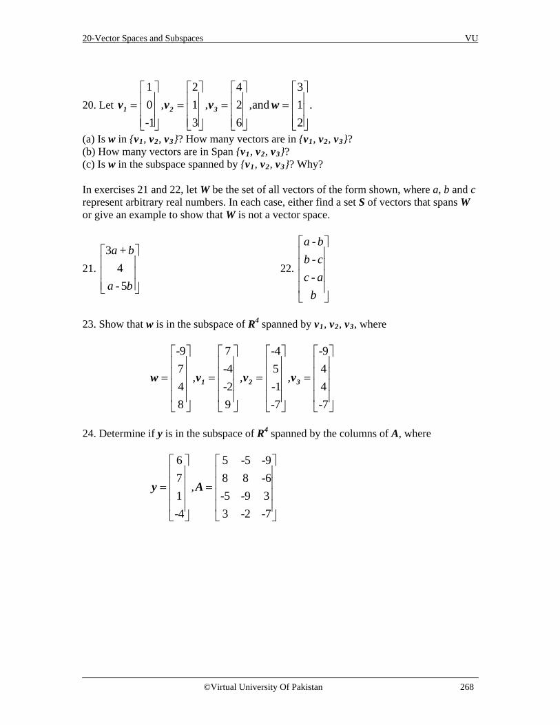
20-Vector Spaces and Subspaces VU
©Virtual University Of Pakistan 268
20. Let 1 2 4 30 1 2 and 1-1 3 6 2
, , , . = = = =
1 2 3v v v w
(a) Is w in {v1, v2, v3}? How many vectors are in {v1, v2, v3}? (b) How many vectors are in Span {v1, v2, v3}? (c) Is w in the subspace spanned by {v1, v2, v3}? Why? In exercises 21 and 22, let W be the set of all vectors of the form shown, where a, b and c represent arbitrary real numbers. In each case, either find a set S of vectors that spans W or give an example to show that W is not a vector space.
21. 3 +
4- 5
a b
a b
22.
---
a bb cc a
b
23. Show that w is in the subspace of R4 spanned by v1, v2, v3, where
-9 7 -4 -97 -4 5 44 -2 -1 48 9 -7 -7
, , ,
= = = =
1 2 3w v v v
24. Determine if y is in the subspace of R4 spanned by the columns of A, where
6 5 -5 -97 8 8 -61 -5 -9 3-4 3 -2 -7
,
= =
y A

21-Null Spaces, Column Spaces and Linear Transformation VU
©Virtual University Of Pakistan 269
Lecture 21
Null Spaces, Column Spaces, and Linear Transformations Subspaces arise in as set of all solutions to a system of homogenous linear equations as the set of all linear combinations of certain specified vectors. In this lecture, we compare and contrast these two descriptions of subspaces, allowing us to practice using the concept of a subspace. In applications of linear algebra, subspaces of Rn usually arise in one of two ways: as the set of all solutions to a system of homogeneous linear equations or as the set of all linear combinations of certain specified vectors.
Our work here will provide us with a deeper understanding of the relationships between the solutions of a linear system of equations and properties of its coefficient matrix. Null Space of a Matrix Consider the following system of homogeneous equations:
1 2 3
1 2 3
3 2 05 9 0
x x xx x x− − =
− + + = (1)
In matrix form, this system is written as Ax = 0, where 1 -3 -2-5 9 1
=
A (2)
Recall that the set of all x that satisfy (1) is called the solution set of the system (1). Often it is convenient to relate this set directly to the matrix A and the equation Ax = 0. We call the set of x that satisfy Ax = 0 the null space of the matrix A. The reason for this name is that if matrix A is viewed as a linear operator that maps points of some vector space V into itself, it can be viewed as mapping all the elements of this solution space of AX = 0 into the null element "0". Thus the null space N of A is that subspace of all vectors in V which are imaged into the null element “0" by the matrix A. NULL SPACE Definition The null space of an m n× matrix A, written as Nul A, is the set of all solutions to the homogeneous equation Ax = 0. In set notation,
Nul A = {x: x is in Rn and Ax = 0} OR
( ) { / , 0}Nul A x x Ax= ∀ ∈ = A more dynamic description of Nul A is the set of all x in Rn that are mapped into the zero vector of Rm via the linear transformation →x Ax , where A is a matrix of transformation. See Figure1

21-Null Spaces, Column Spaces and Linear Transformation VU
©Virtual University Of Pakistan 270
Figure 1
Example 1 Let 1 -3 -2-5 9 1
=
A and let 53 .-2
=
u Determine if Nul∈u A .
Solution To test if u satisfies Au = 0, simply compute
5
1 -3 -2 5 -9 + 4 0= 3 = =
-5 9 1 -25 + 27 - 2 0-2
Au . Thus u is in Nul A.
Example Determine the null space of the following matrix:
4 08 20
A = −
Solution To find the null space of A we need to solve the following system of equations:
We can find Null space of a matrix with two ways i.e. with matrices or with system of linear equations. We have given this in both matrix form and (here first we convert the matrix into system of equations) equation form. In equation form it is easy to see that by solving these equations together the only solution is 1 2 0x x= = . In terms of vectors from
2 the solution consists of the single vector { }0 and hence the null space of A is{ }0 . Activity Determine the null space of the following matrices:
0
Rm Rn
Nul A 0
1
2
1 2
1 2
1 2 1
1 2 2
4 0 08 20 0
4 0 08 20 0
4 0 0 08 20 0 0
xx
x xx x
x x xand x x x
= −
+ ⇒ = − +
⇒ + = ⇒ =⇒ − + = ⇒ =

21-Null Spaces, Column Spaces and Linear Transformation VU
©Virtual University Of Pakistan 271
1
2 1
2
4 0 1 0 1~8 20 8 20 4
1 0~ 8
0 20
1 0 1~0 1 20
R
R R
R
− −
+
1. 0 0 0
0 0 0 00 0 0
=
2. 1 55 25
M−
= −
In earlier (previous) lectures, we developed the technique of elementary row operations to solve a linear system. We know that performing elementary row operations on an augmented matrix does not change the solution set of the corresponding linear system Ax=0. Therefore, we can say that it does not change the null space of A. We state this result as a theorem: Theorem 1 Elementary row operations do not change the null space of a matrix.
Or Null space N(A) of a matrix A can not be changed (always same) by changing the matrix
with elementary row operations. Example Determine the null space of the following matrix using the elementary row operations: (Taking the matrix from the above Example)
4 08 20
A = −
Solution First we transform the matrix to the reduced row echelon form:
which corresponds to the system
1
2
00
xx==
Since every column in the coefficient part of the matrix has a leading entry that means our system has the trivial solution only:
This means the null space consists only of the zero vector. We can observe and compare both the above examples which show the same result.
1
2
00
xx==

21-Null Spaces, Column Spaces and Linear Transformation VU
©Virtual University Of Pakistan 272
Theorem 2 The null space of an m n× matrix A is a subspace of Rn. Equivalently, the set of all solutions to a system Ax = 0 of m homogeneous linear equations in n unknowns is a subspace of Rn. Or simply, the null space is the space of all the vectors of a Matrix A of any order those are mapped (assign) onto zero vector in the space Rn (i.e. Ax = 0). Proof We know that the subspace of A consists of all the solution to the system Ax = 0 . First, we should point out that the zero vector, 0, in Rn will be a solution to this system and so we know that the null space is not empty. This is a good thing since a vector space (subspace or not) must contain at least one element. Now we know that the null space is not empty. Consider u, v be two any vectors (elements) (in) from the null space and let c be any scalar. We just need to show that the sum (u+v) and scalar multiple (c.u) of these are also in the null space. Certainly Nul A is a subset of Rn because A has n columns. To show that Nul(A) is the subspace, we have to check three conditions whether they are satisfied or not. If Nul(A) satisfies the all three condition, we say Nul(A) is a subspace otherwise not. First, zero vector “0” must be in the space and subspace. If zero vector does not in the space we can not say that is a vector space (generally, we use space for vector space). And we know that zero vector maps on zero vector so 0 is in Nul(A). Now choose any vectors u, v from Null space and using definition of Null space (i.e. Ax=0)
Au = 0 and Av = 0
Now the other two conditions are vector addition and scalar multiplication. For this we proceed as follow: Let start with vector addition: To show that u + v is in Nul A, we must show that A (u + v) = 0. Using the property of matrix multiplication, we find that A (u + v) = Au + Av = 0 + 0 = 0 Thus u + v is in Nul A, and Nul A is closed under vector addition. For Matrix multiplication, consider any scalar , say c, A (cu) = c (Au) = c (0) = 0 which shows that cu is in Nul A. Thus Nul A is a subspace of Rn. Example 2 The set H, of all vectors in R4 whose coordinates a, b, c, d satisfy the equations a – 2b + 5c = d c – a = b is a subspace of R4. Solution Since a – 2b + 5c = d c – a = b By rearranging the equations, we get
a - 2b + 5c - d = 0
-a - b + c = 0

21-Null Spaces, Column Spaces and Linear Transformation VU
©Virtual University Of Pakistan 273
We see that H is the set of all solutions of the above system of homogeneous linear equations. Therefore from the Theorem 2, H is a subspace of R4. It is important that the linear equations defining the set H are homogeneous. Otherwise, the set of solutions will definitely not be a subspace (because the zero-vector (origin) is not a solution of a non- homogeneous system), geometrically means that a line that not passes through origin can not be a subspace, because subspace must hold the zero vector (origin). Also, in some cases, the set of solutions could be empty. In this case, we can not find any solution of a system of linear equations, geometrically says that lines are parallel or not intersecting. If the null space having more than one vector, geometrically means that the lines intersect more than one point and must passes through origin (zero vector) . An Explicit Description of Nul A There is no obvious relation between vectors in Nul A and the entries in A. We say that Nul A is defined implicitly, because it is defined by a condition that must be checked. No explicit list or description of the elements in Nul A is given. However, when we solve the equation Ax = 0, we obtain an explicit description of Nul A. Example 3 Find a spanning set for the null space of the matrix
Solution The first step is to find the general solution of Ax = 0 in terms of free variables. After transforming the augmented matrix [A 0] to the reduced row echelon form and we get;
1 -2 0 -1 3 00 0 1 2 -2 00 0 0 0 0 0
which corresponds to the system
1 2 4 5
3 4 5
x - 2x - x + 3x = 0 x + 2x - 2x = 0 0 = 0
The general solution is 1 2 4 5
2
3 4 5
4
5
x = 2x + x - 3xx = free variablex = - 2x + 2xx = free variablex = free variable
- 3 6 -1 1 - 7 1 - 2 2 3 - 1 2 - 4 5 8 - 4
=
A

21-Null Spaces, Column Spaces and Linear Transformation VU
©Virtual University Of Pakistan 274
Next, decompose the vector giving the general solution into a linear combination of vectors where the weights are the free variables. That is,
2 -3 2 1 -31 0 0
-2 2 0 -2 20 1 00 0 1
1 2 4 5
2 2
3 4 5 2 4 5
4 4
5 5
x x + x xx xx = x + x = x + x + xx xx x
↑ ↑ ↑ u v w
2 4 5= x + x + xu v w (3) Every linear combination of u, v and w is an element of Nul A. Thus {u, v, w} is a spanning set for Nul A. Two points should be made about the solution in Example 3 that apply to all problems of this type. We will use these facts later.
1. The spanning set produced by the method in Example 3 is automatically linearly independent because the free variables are the weights on the spanning vectors. For instance, look at the 2nd, 4th and 5th entries in the solution vector in (3) and note that 2 4 5x + x + xu v w can be 0 only if the weights x2, x4 and x5 are all zero.
2. When Nul A contains nonzero vector, the number of vectors in the spanning set for Nul A equals the number of free variables in the equation Ax = 0.
Example 4 Find a spanning set for the null space of
1 -3 2 2 10 3 6 0 -32 -3 -2 4 43 -6 0 6 5-2 9 2 -4 -5
=
A .
Solution The null space of A is the solution space of the homogeneous system 1 2 3 4 5
1 2 3 4 5
1 2 3 4 5
1 2 3 4 5
1 2 3 4 5
x - 3x + 2x + 2x + x = 00x +3x +6x +0x - 3x = 02x - 3x - 2x +4x +4x = 03x - 6x +0x +6x +5x = 0-2x +9x + 2x - 4x - 5x = 0

21-Null Spaces, Column Spaces and Linear Transformation VU
©Virtual University Of Pakistan 275
1 -3 2 2 1 0 0 3 6 0 -3 0 2 -3 -2 4 4 0 3 -6 0 6 5 0-2 9 2 -4 -5 0
1 -3 2 2 1 0 0 3 6 0 -3 0 0 3 - 6 0 2 0 0 3 - 6 0 2 0 0 3 6 0 -3 0
1 3
1 4
1 5
- 2R + R-3R + R2R + R
1 -3 2 2 1 0 0 1 2 0 -1 0 0 3 - 6 0 2 0 0 3 - 6 0 2 0 0 3 6 0 -3 0
2(1/3)R
1 -3 2 2 1 00 1 2 0 -1 00 0 -12 0 5 00 0 -12 0 5 00 0 0 0 0 0
2 3
2 4
2 5
- 3R + R-3R + R-3R + R
1 -3 2 2 1 0 0 1 2 0 -1 0 0 0 1 0 -5/12 0 0 0 -12 0 5 0 0 0 0 0 0 0
3(-1/12)R
1 -3 2 2 1 0 0 1 2 0 -1 0 0 0 1 0 -5/12 0 0 0 0 0 0 0 0 0 0 0 0 0
3 412R + R
1 -3 0 2 11/ 6 0 0 1 0 0 -1/6 0 0 0 1 0 -5/12 0 0 0 0 0 0 0 0 0 0 0 0 0
3 2
3 1
- 2R + R-2R + R

21-Null Spaces, Column Spaces and Linear Transformation VU
©Virtual University Of Pakistan 276
1 0 0 2 4/3 00 1 0 0 -1/6 00 0 1 0 -5/12 00 0 0 0 0 00 0 0 0 0 0
2 13R + R
The reduced row echelon form of the augmented matrix corresponds to the system
1 4 5
2 5
3 5
1 x + 2 x +(4/3) x = 01 x + (-1/6) x = 0
1 x + (-5/12) x = 00 = 00 = 0
.
No equation of this system has a form zero = nonzero; Therefore, the system is consistent. The system has infinitely many solutions:
arbitrary arbitrary1 4 5 2 5 3 5
4 5
x = -2 x +(-4/3) x x = +(1/6) x x = +(5/12) xx = x =
The solution can be written in the vector form:
= (-2,0,0,1,0) = (-4/3,1/6,5/12,0,1)4 5c c
Therefore {(-2,0,0,1,0), (-4/3,1/6,5/12,0,1)} is a spanning set for Null space of A. Activity: Find an explicit description of Nul A where:
1. 3 5 5 3 95 1 1 0 3
A =
2.
4 1 1 0 11 1 2 3 11 1 2 0 10 0 1 1 1
A
− − − − = − −
The Column Space of a Matrix Another important subspace associated with a matrix is its column space. Unlike the null space, the column space is defined explicitly via linear combinations.

21-Null Spaces, Column Spaces and Linear Transformation VU
©Virtual University Of Pakistan 277
Definition (Column Space) The column space of an m n× matrix A, written as Col A, is the set of all linear combinations of the columns of A. If A = [a1 … an], then
Col A = Span {a1 ,… , an } Since Span {a1, …, an } is a subspace, by Theorem of lecture 20 i.e. if 1,..., pv v are in a
vector space V , then Span { }1,..., pv v is a subspace of V . The column space of a matrix is that subspace spanned by the columns of the matrix (columns viewed as vectors). It is that space defined by all linear combinations of the column of the matrix. Example, in the given matrix,
1 1 32 1 43 1 54 1 6
A
=
The column space ColA is all the linear combination of the first (1, 2, 3, 4), the second (1, 1, 1, 1) and the third column ( 3, 4, 5, 6). That is, ColA = { a·(1, 2, 3, 4) + b·(1, 1, 1, 1) + c·( 3, 4, 5, 6) }. In general, the column space ColA contains all the linear combinations of columns of A. The next theorem follows from the definition of Col A and the fact that the columns of A are in Rm. Theorem 3 The column space of an m n× matrix A is a subspace of Rm. Note that a typical vector in Col A can be written as Ax for some x because the notation Ax stands for a linear combination of the columns of A. That is,
Col A = {b: b = Ax for some x in Rn} The notation Ax for vectors in Col A also shows that Col A is the range of the linear transformation .→x Ax
Example 6 Find a matrix A such that W = Col A. 6 -
+-7
a b= a b : a,b in R
a
W
Solution First, write W as a set of linear combinations. 6 -1 6 -11 1 Span 1 , 1-7 0 -7 0
= a +b : a,b in R =
W
Second, use the vectors in the spanning set as the columns of A. Let 6 -11 1-7 0
= .
A
Then W = Col A, as desired.

21-Null Spaces, Column Spaces and Linear Transformation VU
©Virtual University Of Pakistan 278
We know that the columns of A span Rm if and only if the equation Ax = b has a solution for each b. We can restate this fact as follows: The column space of an m n× matrix A is all of Rm if and only if the equation Ax = b has a solution for each b in Rm. Theorem 4 A system of linear equations Ax = b is consistent if and only if b in the column space of A. Example 6 A vector b in the column space of A. Let Ax = b is the linear system
-1 3 2 11 2 -3 = -92 1 -2 -3
1
2
3
xxx
. Show that b is in the column space of A, and express b as a
linear combination of the column vectors of A. Solution Augmented Matrix is given by
-1 3 2 1 1 2 -3 -9 2 1 -2 -3
1 -3 - 2 -10 5 -1 -80 7 2 -1
1
1 2
1 3
-1R-1R + R-2R + R
1 -3 -2 -10 1 -1/5 -8/50 0 17/5 51/5
2
2 3
1/5R-7R + R
1 -3 0 50 1 0 -10 0 1 3
3
3 2
3 1
(5/17)R(1/5)R + R
2R + R
0
x2
x1
x3
W

21-Null Spaces, Column Spaces and Linear Transformation VU
©Virtual University Of Pakistan 279
1 0 0 20 1 0 -10 0 1 3
2 13R + R
1 2 3x = 2,x = -1,x = 3⇒ . Since the system is consistent, b is in the column space of A.
Moreover, -1 3 2 1
2 1 - 2 + 3 -3 = -92 1 -2 -3
Example Determine whether b is in the column space of A and if so, express b as a linear combination of the column vectors of A:
1 1 2 11 0 1 : 02 1 3 2
A b−
= =
Solution The coefficient matrix Ax b= is:
The augmented matrix for the linear system that corresponds to the matrix equation Ax b= is:
1 1 2 11 0 1 02 1 3 2
−
We reduce this matrix to the Reduced Row Echelon Form:
( )
( )
2 1
3 1
1 1 2 1 1 1 2 11 0 1 0 ~ 0 1 1 1 12 1 3 2 2 1 3 2
1 1 2 1~ 0 1 1 1 2
0 1 1 4
R R
R R
− − − − + −
− − − + − − −
( ) 2
1 1 2 1~ 0 1 1 1 1
0 1 1 4R
− − − − −
1
2
3
1 1 2 11 0 1 02 1 3 2
xxx
− =

21-Null Spaces, Column Spaces and Linear Transformation VU
©Virtual University Of Pakistan 280
3 2
1 1 2 1~ 0 1 1 1
0 0 0 3R R
− − +
( )
3
2 3
1 3
1 2
1 1 2 11~ 0 1 1 13
0 0 0 1
1 1 2 1~ 0 1 1 0
0 0 0 1
1 1 2 0~ 0 1 1 0
0 0 0 1
1 0 1 0~ 0 1 1 0 1
0 0 0 1
R
R R
R R
R R
− − − + + + −
The new system for the equation Ax b= is
1 3
2 3
00
0 1
x xx x+ =+ =
=
Equation 0 1= cannot be solved, therefore, the system has no solution (i.e. the system is inconsistent). Since the equation Ax = b has no solution, therefore b is not in the column space of A. Activity Determine whether b is in the column space of A and if so, express b as a linear combination of the column vectors of A:
1.
2. 1 1 1 11 1 1 ; 21 1 1 3
A b−
= − = − − −
1 1 2 59 3 1 ; 11 1 1 0
A b−
= =

21-Null Spaces, Column Spaces and Linear Transformation VU
©Virtual University Of Pakistan 281
3.
1 1 2 1 10 2 0 1 2
;1 1 1 3 30 2 2 1 4
A b
− = = −
Theorem 5 If x0 denotes any single solution of a consistent linear system Ax=b and if
, , ,...,1 2 3 kv v v v form the solution space of the homogeneous system Ax=0, then every solution of Ax=b can be expressed in the form 1 2 ... kc c c= + + + +0 1 2 kx x v v v and, conversely, for all choices of scalars 1 2 3, , ,..., kc c c c , the vector x is a solution of Ax=b. General and Particular Solutions: The vector x0 is called a particular solution of Ax=b .The expression x0+ c1 v1 +c2v2+ . . . +ck vk is called the general solution of Ax=b , and the expression c1 v1 +c2v2+ . . . +ck vk is called the general solution of Ax=0. Example 7 Find the vector form of the general solution of the given linear system Ax = b; then use that result to find the vector form of the general solution of Ax=0.
1 2 3 5
1 2 3 4 5 6
3 4 6
1 2 4 5 6
x +3x - 2x + 2x = 02x +6x - 5x - 2x +4x - 3x = -1
5x +10x +15x = 52x +6x +8x +4x +18x = 6
Solution We solve the non-homogeneous linear system. The augmented matrix of this system is given by
1 3 -2 0 2 0 02 6 -5 -2 4 -3 -10 0 5 10 0 15 52 6 0 8 4 18 6
1 3 - 2 0 2 0 0 0 0 -1 - 2 0 -3 -1 0 0 5 10 0 15 5 0 0 4 8 0 18 6
1 2
1 4
-2R + R-2R + R
2
1 3 - 2 0 2 0 0 0 0 1 2 0 3 1 0 0 5 10 0 15 5 0 0 4 8 0 18 6
-1R

21-Null Spaces, Column Spaces and Linear Transformation VU
©Virtual University Of Pakistan 282
1 3 - 2 0 2 0 0 0 0 1 2 0 3 1 0 0 0 0 0 0 0 0 0 0 0 0 6 2
2 3
2 4
-5R + R-4R + R
34
1 3 - 2 0 2 0 0 0 0 1 2 0 3 1 0 0 0 0 0 6 2 0 0 0 0 0 0 0
R
1 3 - 2 0 2 0 0 0 0 1 2 0 3 1 0 0 0 0 0 1 1/3 0 0 0 0 0 0 0
3(1/6)R
1 3 - 2 0 2 0 0 0 0 1 2 0 0 0 0 0 0 0 0 1 1/3 0 0 0 0 0 0 0
3 2- 3R + R
1 3 0 4 2 0 0 0 0 1 2 0 0 0 0 0 0 0 0 1 1/3 0 0 0 0 0 0 0
2 12R + R
The reduced row echelon form of the augmented matrix corresponds to the system
1 2 4 5
3 4
6
1 x +3 x + 4 x +2 x = 01 x +2 x = 0
1 x = (1/3) 0 = 0
No equation of this system has a form zero = nonzero; Therefore, the system is consistent. The system has infinitely many solutions:
1 2 4 5 2 3 4
4 5 6
x = -3 x - 4 x - 2 x x = r x = -2 xx = s x = t x = 1/3
1 2 3
4 5 6
x = -3r - 4s - 2t x = r x = -2s1x = s x = t x =3

21-Null Spaces, Column Spaces and Linear Transformation VU
©Virtual University Of Pakistan 283
This result can be written in vector form as -3 - 4 - 2 0 -3 -4 -2
0 1 0 0-2 0 0 -2 0
0 0 1 00 0 0 1
1 1 0 0 03 3
1
2
3
4
5
6
r s txrxsx
= = + r + s +tsxtx
x
(A)
which is the general solution of the given system. The vector x0 in (A) is a particular
solution of the given system; the linear combination
-3 -4 -21 0 00 -2 00 1 00 0 10 0 0
r + s +t
in (A) is the
general solution of the homogeneous system. Activity:
1. Suppose that 1 2 3 41, 2, 4, 3x x x x= − = = = − is a solution of a non-homogenous linear system Ax b= and that the solution set of the homogenous system 0Ax = is given by this formula:
1
2
3
4
3 4 ,,
,
x r sx r sx rx s
= − += −==
(a) Find the vector form of the general solution of 0Ax = . (b) Find the vector form of the general solution of 0Ax = .
Find the vector form of the general solution of the following linear system Ax = b; then use that result to find the vector form of the general solution of Ax=0:
2. 1 2
1 2
2 13 9 2
x xx x− =− =
3.
1 2 3 4
1 2 3 4
1 2 3 4
1 2 4
2 3 33 3 1
3 2 24 5 3 5
x x x xx x x xx x x xx x x
+ − + =− − + + = −
− + − + =− − = −

21-Null Spaces, Column Spaces and Linear Transformation VU
©Virtual University Of Pakistan 284
The Contrast between Nul A and Col A It is natural to wonder how the null space and column space of a matrix are related. In fact, the two spaces are quite dissimilar. Nevertheless, a surprising connection between the null space and column space will emerge later.
Example 8 Let 2 4 -2 1
= -2 -5 7 33 7 -8 6
A
(a) If the column space of A is a subspace of Rk, what is k? (b) If the null space of A is a subspace of Rk, what is k? Solution (a) The columns of A each have three entries, so Col A is a subspace of Rk, where k = 3. (b) A vector x such that Ax is defined must have four entries, so Nul A is a subspace of Rk, where k = 4. When a matrix is not square, as in Example 8, the vectors in Nul A and Col A live in entirely different “universes”. For example, we have discussed no algebraic operations that connect vectors in R3 with vectors in R4. Thus we are not likely to find any relation between individual vectors in Nul A and Col A.
Example 9 If2 4 -2 1
= -2 -5 7 33 7 -8 6
A , find a nonzero vector in Col A and a nonzero vector
in Nul A
Solution It is easy to find a vector in Col A. Any column of A will do, say, 2-23
.
To
find a nonzero vector in Nul A, we have to do some work. We row reduce the augmented
matrix [A 0] to obtain1 0 9 0 0
[ ] ~ 0 1 -5 0 00 0 0 1 0
A 0 . Thus if x satisfies Ax = 0,
then 1 3 2 3 4x = -9x , x = 5x , x = 0 , and x3 is free. Assigning a nonzero value to x3 (say), x3 = 1, we obtain a vector in Nul A, namely, x = (-9, 5, 1, 0).
Example 10 With2 4 -2 1-2 -5 7 33 7 -8 6
=
A , let
33
-2and -1
-13
0
= = .
u v
(a) Determine if u is in Nul A. Could u be in Col A?

21-Null Spaces, Column Spaces and Linear Transformation VU
©Virtual University Of Pakistan 285
(b) Determine if v is in Col A. Could v be in Nul A? Solution (a) An explicit description of Nul A is not needed here. Simply compute the product
32 4 -2 1 0 0
-2= -2 -5 7 3 = -3 0
-13 7 -8 6 3 0
0
≠
Au
Obviously, u is not a solution of Ax = 0, so u is not in Nul A. Also, with four entries, u could not possibly be in Col A, since Col A is a subspace of R3. (b) Reduce [A v] to an echelon form:
2 4 -2 1 3 2 4 -2 1 3[ ] -2 -5 7 3 -1 0 1 -5 -4 2
3 7 -8 6 3 0 0 0 17 1
=
A v
At this point, it is clear that the equation Ax = v is consistent, so v is in Col A. With only three entries, v could not possibly be in Nul A, since Nul A is a subspace of R4. The following table summarizes what we have learned about Nul A and Col A.
1. Nul A is a subspace of Rn. 2. Nul A is implicitly defined; i.e. we
are given only a condition (Ax = 0) that vectors in Nul A must satisfy.
3. It takes time to find vectors in Nul A. Row operations on [A 0] are required.
4. There is no obvious relation between Nul A and the entries in A.
5. A typical vector v in Nul A has the
property that Av = 0. 6. Given a specific vector v, it is easy
to tell if v is in Nul A. Just compute Av.
7. Nul A = {0} if and only if the
equation Ax = 0 has only the trivial solution.
8. Nul A = {0} if and only if the linear transformation →x Ax is one-to-one.
1. Col A is a subspace of Rm. 2. Col A is explicitly defined; that is,
we are told how to build vectors in Col A.
3. It is easy to find vectors in Col A The columns of A are displayed; others are formed from them.
4. There is an obvious relation between Col A and the entries in A, since each column of A is in Col A.
5. A typical vector v in Col A has the property that the equation Ax = v is consistent.
6. Given a specific vector v, it may take time to tell if v is in Col A. Row operations on [A v] are required.
7. Col A.= Rm if and only if the equation Ax = b has a solution for every b in Rm.
8. Col A = Rm if and only if the linear transformation →x Ax maps Rn onto Rm.

21-Null Spaces, Column Spaces and Linear Transformation VU
©Virtual University Of Pakistan 286
Kernel and Range of A Linear Transformation Subspaces of vector spaces other than Rn are often described in terms of a linear transformation instead of a matrix. To make this precise, we generalize the definition given earlier in Segment I. Definition A linear transformation T from a vector space V into a vector space W is a rule that assigns to each vector x in V a unique vector T (x) in W, such that
(i) T (u + v) = T (u) + T (v) for all u, v in V, and (ii) T (cu) = c T (u) for all u in V and all scalars c. The kernel (or null space) of such a T is the set of all u in V such that T (u) = 0 (the zero vector in W). The range of T is the set of all vectors in W of the form T (x) for some x in V. If T happens to arise as a matrix transformation, say, T (x) = Ax for some matrix A – then the kernel and the range of T are just the null space and the column space of A, as defined earlier. So if T(x) = Ax, col A = range of T. Definition If :T V W→ is a linear transformation, then the set of vectors in V that T maps into 0 is called the kernel of T; it is denoted by ker(T). The set of all vectors in W that are images under T of at least one vector in V is called the range of T; it is denoted by R(T). Example If : n m
AT → is multiplication by the m n× matrix A, then from the above definition; the kernel of AT is the null space of A and the range of AT is the column space of A. Remarks The kernel of T is a subspace of V and the range of T is a subspace of W.
Figure 2 Subspaces associated with a linear transformation.
In applications, a subspace usually arises as either the kernel or the range of an appropriate linear transformation. For instance, the set of all solutions of a homogeneous linear differential equation turns out to be the kernel of a linear transformation. Typically, such a linear transformation is described in terms of one or more derivatives of a
0 W
V’ 0
Range
Kernel
Domain
Kernel is a subspace of V
Range is a subspace of W

21-Null Spaces, Column Spaces and Linear Transformation VU
©Virtual University Of Pakistan 287
function. To explain this in any detail would take us too far a field at this point. So we present only two examples. The first explains why the operation of differentiation is a linear transformation. Example 11 Let V be the vector space of all real-valued functions f defined on an interval [a, b] with the property that they are differentiable and their derivatives are continuous functions on [a, b]. Let W be the vector space of all continuous functions on [a, b] and let : →D V W be the transformation that changes f in V into its derivative ′f . In calculus, two simple differentiation rules are ( ) ( ) ( ) and ( ) ( )c c+ = + =D f g D f D g D f D f That is, D is a linear transformation. It can be shown that the kernel of D is the set of constant functions of [a, b] and the range of D is the set W of all continuous functions on [a, b]. Example 12 The differential equation 0y wy′′ + = (4) where w is a constant, is used to describe a variety of physical systems, such as the vibration of a weighted spring, the movement of a pendulum and the voltage in an inductance – capacitance electrical circuit. The set of solutions of (4) is precisely the kernel of the linear transformation that maps a function ( )=y f t into the function ( ) ( )w′′ +f t f t . Finding an explicit description of this vector space is a problem in differential equations.
Example 13 Let .a
= b : a - 3b - c = 0c
W Show that W is a subspace of R3 in
different ways. Solution First method: W is a subspace of R3 by Theorem 2 because W is the set of all solutions to a system of homogeneous linear equations (where the system has only one equation). Equivalently, W is the null space of the 1x3 matrix = [1 - 3 -1].A Second method: Solve the equation a – 3b – c = 0 for the leading variable a in terms of the free variables b and c.
Any solution has the form 3
,b+cbc
where b and c are arbitrary, and
3 3 11 00 1
b+cb = b +cc
↑ ↑
1 2v v

21-Null Spaces, Column Spaces and Linear Transformation VU
©Virtual University Of Pakistan 288
This calculation shows that W = Span{v1, v2}. Thus W is a subspace of R3 by Theorem i.e. if 1,..., pv v are in a vector spaceV , then Span { }1,..., pv v is a subspace ofV . We could also solve the equation a – 3b – c = 0 for b or c and get alternative descriptions of W as a set of linear combinations of two vectors.
Example 14 Let7 -3 5 2 7-4 1 -5 1 6-5 2 -4 -1 -3
= , = ,and =
A v W
Suppose you know that the equations Ax = v and Ax = w are both consistent. What can you say about the equation Ax = v + w? Solution Both v and w are in Col A. Since Col A is a vector space, v + w must be in Col A. That is, the equation Ax = v + w is consistent. Activity
1. Let V and W be any two vector spaces. The mapping :T V W→ such that T (v) = 0 for every v in V is a linear transformation called the zero transformation. Find the kernel and range of the zero transformation.
2. Let V be any vector space. The mapping :I V V→ defined by I(v) = v is called
the identity operator on V. Find the kernel and range of the identity operator.

21-Null Spaces, Column Spaces and Linear Transformation VU
©Virtual University Of Pakistan 289
Exercises
1. Determine if w = 5-32
is in Nul A, where A=5 21 19
13 23 28 14 1
.
In exercises 2 and 3, find an explicit description of Nul A, by listing vectors that span the null space.
2. 1 3 5 00 1 4 -2
3. 1 -2 0 4 00 0 1 -9 00 0 0 0 1
In exercises 4-7, either use an appropriate theorem to show that the given set, W is a vector space, or find a specific example to the contrary.
4. :ab a+b+c = 2c
5. :
ab a - 2b = 4cc 2a = c+3dd
6.
- 25 +
: real+ 3
b dd
b,db d
d
7. - + 2
- 2 : real3 - 6
a ba b a,ba b
In exercises 8 and 9, find A such that the given set is Col A.
8.
2 + 3- 2
: real4 +
3 - -
s tr s t
r,s,tr s
r s t
+
9.
-2 +
: , , real5 - 4
b cb c d
b c dc d
d
+
For the matrices in exercises 10-13, (a) find k such that Nul A is a subspace of Rk, and (b) find k such that Col A is a subspace of Rk.

21-Null Spaces, Column Spaces and Linear Transformation VU
©Virtual University Of Pakistan 290
10.
2 -6-1 3-4 123 -9
=
A 11.
7 -2 0-2 0 -50 -5 7-5 7 -2
=
A
12. A=4 5 -2 6 01 1 0 1 0
13. A=[ ]1 -3 9 0 -5
14. Let-6 12 2
and-3 6 1
= =
A w . Determine if w is in Col A. Is w in Nul A?
15. Let -8 -2 -9 26 4 8 and 14 0 4 -2
= =
A w . Determine if w is in Col A. Is w in Nul A?
16. Define T: P2→R2 by T (p) = (0)(1)
pp
. For instance, if p (t) = 3 + 5t + 7t2, then
315
( ) =
T p .
a. Show that T is a linear transformation. b. Find a polynomial p in P2 that spans the kernel of T, and describe the range of T.
17. Define a linear transformation T: P2→R2 by T (p) =(0)(1)
pp
. Find polynomials p1
and p2 in P2 that span the kernel of T, and describe the range of T. 18. Let M2x2 be the vector space of all 2x2 matrices, and define T: M2x2→ M2x2 by
T (A) = A + AT, where a bc d
=
A .
(a) Show that T is a linear transformation. (b) Let B be any element of M2x2 such that BT=B. Find an A in M2x2 such that T (A) = B. (c) Show that the range of T is the set of B in M2x2 with the property that BT=B. (d) Describe the kernel of T. 19. Determine whether w is in the column space of A, the null space of A, or both, where

21-Null Spaces, Column Spaces and Linear Transformation VU
©Virtual University Of Pakistan 291
(a)
1 7 6 -4 11 -5 -1 0 -2-1 9 -11 7 -3-3 19 -9 7 1
,
= =
w A (b)
1 -8 5 -2 02 -5 2 1 -21 10 -8 6 -30 3 -2 1 0
,
= =
w A
20. Let a1, …, a5 denote the columns of the matrix A, where
5 1 2 2 03 3 2 -1 -128 4 4 -5 122 1 1 0 -2
=
A , [ ]= 1 2 4B a a a
(a) Explain why a3 and a5 are in the column space of B (b) Find a set of vectors that spans Nul A (c) Let T: R5→R4 be defined by T (x) = Ax. Explain why T is neither one-to-one nor onto.

22- Linear Independence Sets; Bases VU
©Virtual University Of Pakistan 292
Lecture 22
Linearly Independent Sets; Bases First we revise some definitions and theorems from the Vector Space: Definition Let V be an arbitrary nonempty set of objects on which two operations are defined, addition and multiplication by scalars. If the following axioms are satisfied by all objects u, v, w in V and all scalars l and m, then we call V a vector space. Axioms of Vector Space For any set of vectors u, v, w in V and scalars l, m, n: 1. u + v is in V 2. u + v = v + u 3. u + (v + w) = (u + v) + w 4. There exist a zero vector 0 such that 0 + u = u + 0 = u 5. There exist a vector – u in V such that -u + u = 0 = u + (-u) 6. (l u) is in V 7. l (u + v)= l u + l v 8. m (n u) = (m n) u = n (m u) 9. (l +m) u= I u+ m u 10. 1u = u where 1 is the multiplicative identity Definition A subset W of a vector space V is called a subspace of V if W itself is a vector space under the addition and scalar multiplication defined on V. Theorem If W is a set of one or more vectors from a vector space V, then W is subspace of V if and only if the following conditions hold: (a) If u and v are vectors in W, then u + v is in W (b) If k is any scalar and u is any vector in W, then k u is in W. Definition The null space of an m x n matrix A (Nul A) is the set of all solutions of the hom equation Ax = 0 Nul A = {x: x is in Rn and Ax = 0} Definition The column space of an m x n matrix A (Col A) is the set of all linear combinations of the columns of A. If A = [a1 … an], then Col A = Span { a1,… , an }
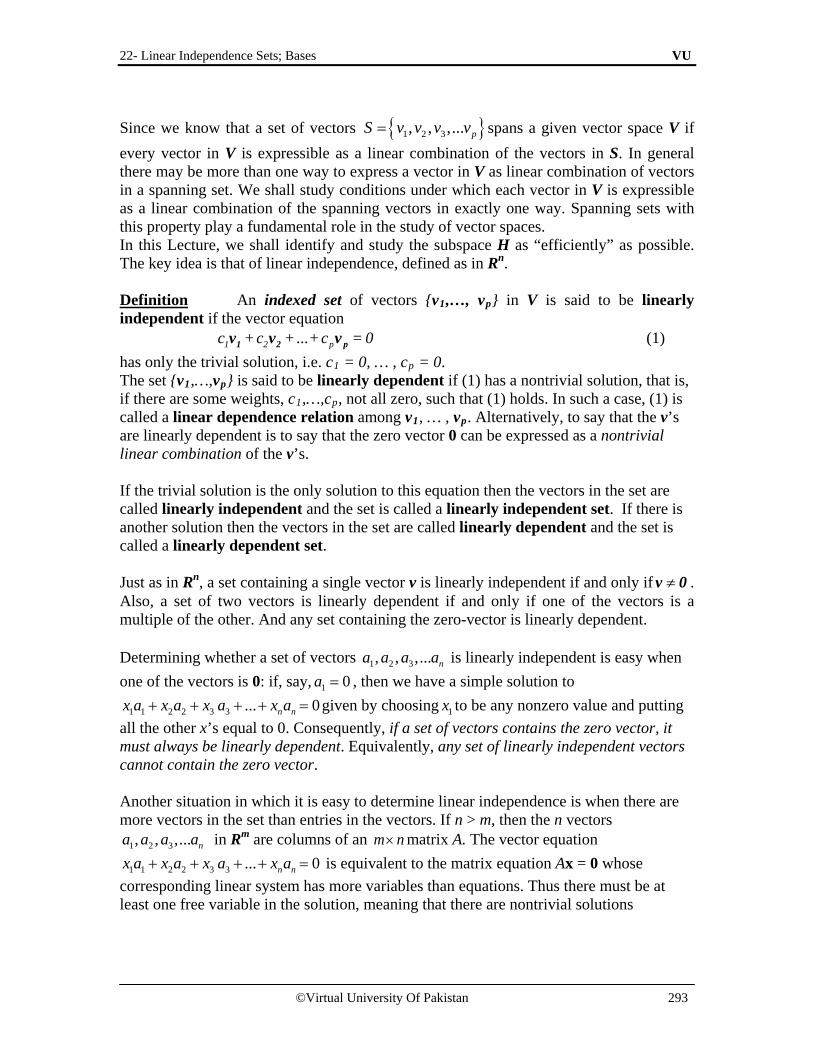
22- Linear Independence Sets; Bases VU
©Virtual University Of Pakistan 293
Since we know that a set of vectors { }1 2 3, , ,... pS v v v v= spans a given vector space V if every vector in V is expressible as a linear combination of the vectors in S. In general there may be more than one way to express a vector in V as linear combination of vectors in a spanning set. We shall study conditions under which each vector in V is expressible as a linear combination of the spanning vectors in exactly one way. Spanning sets with this property play a fundamental role in the study of vector spaces. In this Lecture, we shall identify and study the subspace H as “efficiently” as possible. The key idea is that of linear independence, defined as in Rn. Definition An indexed set of vectors {v1,…, vp} in V is said to be linearly independent if the vector equation
1 2 pc +c +...+c = 01 2 pv v v (1) has only the trivial solution, i.e. c1 = 0, … , cp = 0. The set {v1,…,vp} is said to be linearly dependent if (1) has a nontrivial solution, that is, if there are some weights, c1,…,cp, not all zero, such that (1) holds. In such a case, (1) is called a linear dependence relation among v1, … , vp. Alternatively, to say that the v’s are linearly dependent is to say that the zero vector 0 can be expressed as a nontrivial linear combination of the v’s. If the trivial solution is the only solution to this equation then the vectors in the set are called linearly independent and the set is called a linearly independent set. If there is another solution then the vectors in the set are called linearly dependent and the set is called a linearly dependent set. Just as in Rn, a set containing a single vector v is linearly independent if and only if ≠v 0 . Also, a set of two vectors is linearly dependent if and only if one of the vectors is a multiple of the other. And any set containing the zero-vector is linearly dependent. Determining whether a set of vectors 1 2 3, , ,... na a a a is linearly independent is easy when one of the vectors is 0: if, say, 1 0a = , then we have a simple solution to
1 1 2 2 3 3 ... 0n nx a x a x a x a+ + + + = given by choosing 1x to be any nonzero value and putting all the other x’s equal to 0. Consequently, if a set of vectors contains the zero vector, it must always be linearly dependent. Equivalently, any set of linearly independent vectors cannot contain the zero vector. Another situation in which it is easy to determine linear independence is when there are more vectors in the set than entries in the vectors. If n > m, then the n vectors
1 2 3, , ,... na a a a in Rm are columns of an m n× matrix A. The vector equation
1 1 2 2 3 3 ... 0n nx a x a x a x a+ + + + = is equivalent to the matrix equation Ax = 0 whose corresponding linear system has more variables than equations. Thus there must be at least one free variable in the solution, meaning that there are nontrivial solutions

22- Linear Independence Sets; Bases VU
©Virtual University Of Pakistan 294
to 1 1 2 2 3 3 ... 0n nx a x a x a x a+ + + + = : If n > m, then the set { }1 2 3, , ,... na a a a of vectors in Rm must be linearly dependent. When n is small we have a clear geometric picture of the relation amongst linearly independent vectors. For instance, the case n = 1 produces the equation 1 1 0x a = , and as long as 1 0a ≠ , we only have the trivial solution 1 0x = . A single nonzero vector always forms a linearly independent set. When n = 2, the equation takes the form 1 1 2 2 0x a x a+ = . If this were a linear dependence relation, then one of the x’s, say 1x , would have to be nonzero. Then we could solve the equation for 1a and obtain a relation indicating that 1a is a scalar multiple of 2a . Conversely, if one of the vectors is a scalar multiple of the other, we can express this in the form 1 1 2 2 0x a x a+ = . Thus, a set of two nonzero vectors is linearly dependent if and only if they are scalar multiples of each other. Example (linearly independent set) Show that the following vectors are linearly independent:
1 2 3
2 2 01 , 1 , 01 2 1
v v v− = = = −
Solution Let there exist scalars 1 2 3, ,c c c in R such that
1 1 3 2 3 3 0c v c v c v+ + = Therefore,
1 2 3
2 2 01 1 0 01 2 1
c c c− ⇒ + + = −
1 2
1 2
31 2
2 2 00 0
2
c cc c
cc c
− ⇒ + + = −
1 2
1 2
1 2 3
2 2 0002
c cc cc c c
− + ⇒ + = − +
The above can be written as:
1 2 1 2
1 2
1 2 3
2 2 0 ........(1) 0........(4) ( 2 (1))0 .......(2)
2 0 ......(3)
c c c c dividing by onboth sides ofc cc c c
− + = ⇒ − + =+ =− + =

22- Linear Independence Sets; Bases VU
©Virtual University Of Pakistan 295
1 2
1 23
13
2 1
2
1 2 3 1 2 3
(2) (4) :0
(3) :0 (2) :
0 0 0__________ 0 0
00 2 0 0
00 ; , ,
The system has trivial solution.
Solving and impliesc c
Solving impliesc c Solving implies
cc
cc cc
c c c scalars c c c R are all zero
Hence
+ =− + =
+ + =+ =
⇒ =+ = ⇒ =⇒ =
⇒ = = = ∈
∴
1 2 3, , .the given vectors v v v are linearly independent
Example (linearly dependent set) If { } { } { }1 2 32, 1,0,3 , 1, 2,5, 1 7, 1,5,8v v and v= − = − = − , then the set of vectors
{ }1 2 3, ,S v v v= is linearly dependent, since 1 2 33 0v v v+ − = Example (linearly dependent set) The polynomials 2 2
1 2 31, 2 3 5, 3 1p x p x x and p x x= − + = − + + = − + + form a linearly dependent set in 2p since 1 2 33 2 0p p p− + = . Note The linearly independent or linearly dependent sets can also be determined using the Echelon Form or the Reduced Row Echelon Form methods. Theorem 1 An indexed set { v1, … , vp } of two or more vectors, with ≠1v 0 , is linearly dependent if and only if some vj (with 1j > ) is a linear combination of the preceding vectors, v1, … , vj-1. The main difference between linear dependence in Rn and in a general vector space is that when the vectors are not n – tuples, the homogeneous equation (1) usually cannot be written as a system of n linear equations. That is, the vectors cannot be made into the columns of a matrix A in order to study the equation Ax = 0. We must rely instead on the definition of linear dependence and on Theorem 1. Example 1 Let p1 (t) = 1, p 2(t) = t and p 3 (t) = 4 – t. Then { p 1, p 2, p 3} is linearly dependent in P because p3 = 4p1 – p2. Example 2 The set {Sin t, Cos t} is linearly independent in C [0, 1] because Sin t and Cos t are not multiples of one another as vectors in C [0, 1]. That is, there is no scalar c such that Cos t = c. Sin t for all t in [0, 1]. (Look at the graphs of Sin t and Cos t.) However, {Sin t Cos t, Sin 2t} is linearly dependent because of he identity: Sin 2t = 2 Sin t Cos t, for all t.

22- Linear Independence Sets; Bases VU
©Virtual University Of Pakistan 296
Useful results • A set containing the zero vector is linearly dependent. • A set of two vectors is linearly dependent if and only if one is a multiple of the
other. • A set containing one nonzeoro vector is linearly independent. i.e. consider the set
containing one nonzeoro vector { }1v so { }1v is linearly independent when 1 0v ≠ . • A set of two vectors is linearly independent if and only if neither of the vectors is
a multiple of the other. Activity Determine whether the following sets of vectors are linearly independent or linearly dependent:
1. ( ) ( ) ( )1,0,0,0 , 0,1,0,0 , 0,0,0,1i j k= = = in 4 . 2. ( ) ( ) ( ) ( )1 2 3 42,0, 1 , 3, 2, 5 , 6,1, 1 , 7,0,2v v v v= − = − − − = − − = − in 3.
3. ( ) ( ) ( )1,0,0,...,0 , 0,1,0,...,0 , 0,0,0,...,1i j k= = = in m.
4. 2 2 2 23 3 1, 4 , 3 6 5, 2 7x x x x x x x x+ + + + + − + + in 2p
Definition Let H be a subspace of a vector space V. An indexed set of vectors B = {b1,…, bp} in V is a basis for H if
(i) B is a linearly independent set, and (ii) the subspace spanned by B coincides with H; that is,
H = Span {b1,...,bp } The definition of a basis applies to the case when H = V, because any vector space is a subspace of itself. Thus a basis of V is a linearly independent set that spans V. Observe that when ≠H V , condition (ii) includes the requirement that each of the vectors b1,...,bp must belong to H, because Span { b1,...,bp } contains b1,…,bp, as we saw in lecture 21. Example 3 Let A be an invertible n n× matrix – say, A = [a1 … an]. Then the columns of A form a basis for Rn because they are linearly independent and they span Rn, by the Invertible Matrix Theorem. Example 4 Let e1,…, en be the columns of the n n× identity matrix, In. That is,
1 0 00 1 0
, , ...
0 0 1
= =
=
1 2 ne e e
The set {e1, …, en} is called the standard basis for R n (Fig. 1).
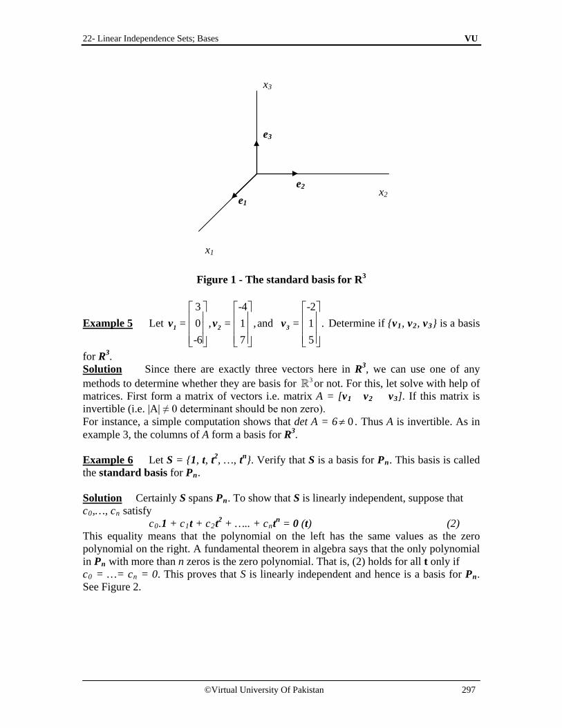
22- Linear Independence Sets; Bases VU
©Virtual University Of Pakistan 297
Figure 1 - The standard basis for R3
Example 5 Let 3 -4 -20 , 1 ,and 1 .-6 7 5
= = =
1 2 3v v v Determine if {v1, v2, v3} is a basis
for R3. Solution Since there are exactly three vectors here in R3, we can use one of any methods to determine whether they are basis for 3
or not. For this, let solve with help of matrices. First form a matrix of vectors i.e. matrix A = [v1 v2 v3]. If this matrix is invertible (i.e. |A| ≠ 0 determinant should be non zero). For instance, a simple computation shows that det A = 6 0≠ . Thus A is invertible. As in example 3, the columns of A form a basis for R3. Example 6 Let S = {1, t, t2, …, tn}. Verify that S is a basis for Pn. This basis is called the standard basis for Pn. Solution Certainly S spans Pn. To show that S is linearly independent, suppose that c0,…, cn satisfy
c0.1 + c1t + c2t2 + ….. + cntn = 0 (t) (2) This equality means that the polynomial on the left has the same values as the zero polynomial on the right. A fundamental theorem in algebra says that the only polynomial in Pn with more than n zeros is the zero polynomial. That is, (2) holds for all t only if c0 = …= cn = 0. This proves that S is linearly independent and hence is a basis for Pn. See Figure 2.
x1
x2
x3
e1 e2
e3

22- Linear Independence Sets; Bases VU
©Virtual University Of Pakistan 298
Figure 2 – The standard basis for P2 Problems involving linear independence and spanning in Pn are handled best by a technique to be discussed later. Example 7 Check whether the set of vectors {(2, -3, 1), (4, 1, 1), (0, -7, 1)} is basis for R3? Solution The set S = {v1, v2, v3} of vectors in R3 spans V = R3 if
c1v1 + c2v2 + c3v3 = d1w1 + d2w2 + d3w3 (*) with w1 = (1,0,0), w2 = (0,1,0) , w3 = (0,0,1) has at least one solution for every set of values of the coefficients d1, d2, d3. Otherwise (i.e., if no solution exists for at least some values of d1, d2, d3), S does not span V. With our vectors v1, v2, v3, (*) becomes
c1(2,-3,1) + c2(4,1,1) + c3(0,-7,1) = d1(1,0,0) + d2(0,1,0) + d3(0,0,1) Rearranging the left hand side yields
1 2 3 1 2 3
1 2 3 1 2 3
1 2 3 1 2 3
2 c +4 c +0 c = 1 d +0 d +0 d-3 c +1 c -7 c = 0 d +1 d +0 d1 c +1 c +1 c = 0 d +0 d +1 d
(A)
2 4 0-3 1 -71 1 1
1 1
2 2
3 3
c dc dc d
⇒ =
We now find the determinant of coefficient matrix 2 4 0-3 1 -71 1 1
to determine whether the
system is consistent (so that S spans V), or inconsistent (S does not span V).
y=1
y=t y=t2
y
t

22- Linear Independence Sets; Bases VU
©Virtual University Of Pakistan 299
Now det 2 4 0-3 1 -71 1 1
= 2(8) – 4(4) +0 = 0
Therefore, the system (A) is inconsistent, and, consequently, the set S does not span the space V. Example 8 Check whether the set of vectors {-4 + 1 t + 3 t2 , 6 + 5 t + 2 t2 , 8 + 4 t + 1 t2} is a basis for P2? Solution The set S = {p1 (t), p2 (t), p3 (t)} of vectors in P2 spans V = P2 if
c1 p1 (t) + c2 p2 (t) + c3 p3 (t) = d1 q1 (t) + d2 q2 (t) + d3 q3 (t) (*) with q1(t) = 1 + 0 t + 0 t 2 , q2(t) = 0 + 1 t + 0 t 2 , q3(t) = 0 + 0 t + 1 t 2 has at least one solution for every set of values of the coefficients d1, d2, d3. Otherwise (i.e., if no solution exists for at least some values of d1, d2, d3), S does not span V. With our vectors p1(t), p2(t), p3(t), (*) becomes:
c1 (-4 + 1 t + 3 t2) + c2 (6 + 5 t + 2 t2) + c3 (8 + 4 t + 1 t2) = d1 (1 + 0 t + 0 t 2 ) + d2 (0 + 1 t + 0 t 2 ) + d3 (0 + 0 t + 1 t 2 )
Rearranging the left hand side yields (-4 c1 +6 c2 +8 c3)1 + (1 c1 +5 c2 +4 c3) t + (3 c1 +2 c2 +1 c3) t2 = (1 d1 +0 d2 +0 d3)1 + (0 d1 +1 d2 +0 d3) t + (0 d1 +0 d2 +1 d3) t2
In order for the equality above to hold for all values of t, the coefficients corresponding to the same power of t on both sides of the equation must be equal. This yields the following system of equations:
1 2 3 1 2 3
1 2 3 1 2 3
1 2 3 1 2 3
-4 c +6 c +8 c = 1 d +0 d +0 d1 c +5 c +4 c = 0 d +1 d +0 d3 c +2 c +1 c = 0 d +0 d +1 d
(A)
- 4 6 81 5 43 2 1
1 1
2 2
3 3
c dc dc d
⇒ =
We now find the determinant of coefficient matrix - 4 6 81 5 43 2 1
to determine whether the
system is consistent (so that S spans V), or inconsistent (S does not span V).
Now det - 4 6 81 5 43 2 1
= -26≠ 0. Therefore, the system (A) is consistent, and,
consequently, the set S spans the space V. The set S = {p1 (t), p2 (t), p3 (t)} of vectors in P2 is linearly independent if the only solution of
c1 p1 (t) + c2 p2 (t) + c3 p3 (t) = 0 (**)

22- Linear Independence Sets; Bases VU
©Virtual University Of Pakistan 300
is c1, c2, c3 = 0. In this case, the set S forms a basis for span S. Otherwise (i.e., if a solution with at least some nonzero values exists), S is linearly dependent. With our vectors p1 (t), p2 (t), p3 (t), (2) becomes: c1 (-4 + 1 t + 3 t2) + c2 (6 + 5 t + 2 t2) + c3 (8 + 4 t + 1 t2) = 0 Rearranging the left hand side yields
(-4 c1 +6 c2 +8 c3)1 + (1 c1 +5 c2 +4 c3) t + (3 c1 +2 c2 +1 c3) t2 = 0 This yields the following homogeneous system of equations:
1 2 3
1 2 3
1 2 3
-4 c +6 c +8 c = 01 c +5 c +4 c = 03 c +2 c +1 c = 0
- 4 6 81 5 43 2 1
1
2
3
c 0c 0
0c
⇒ =
As det - 4 6 81 5 43 2 1
= -26≠ 0. Therefore the set S = {p1 (t), p2 (t), p3 (t)} is linearly
independent. Consequently, the set S forms a basis for span S.
Example 9 The set 1 0 0 1 0 0 0 0
= , , ,0 0 0 0 1 0 0 1
S is a basis for the vector
space V of all 2 x 2 matrices. Solution To verify that S is linearly independent, we form a linear combination of the vectors in S and set it equal to zero:
c1 1 00 0
+ c20 10 0
+ c3 0 01 0
+ c4 0 00 1
= 0 00 0
This gives 0 00 0
1 2
3 4
c c=
c c
, which implies that c1 = c2 = c3 = c4 = 0. Hence S is
linearly independent.
To verify that S spans V we take any vector a bc d
in V and we must find scalars c1, c2,
c3, and c4 such that
c1 1 00 0
+ c20 10 0
+ c3 0 01 0
+ c4 0 00 1
=a bc d
⇒ 1 2
3 4
c c a b=
c c c d
We find that c1 = a, c2 = b, c3 = c, and c4 = d so that S spans V. The basis S in this example is called the standard basis for M22. More generally, the standard basis for Mmn consists of mn different matrices with a single 1 and zeros for the remaining entries Example 10 Show that the set of vectors
3 6 0 -1 0 -8 1 0, , ,
3 -6 -1 0 -12 -4 -1 2
is a basis for the vector space V of all 2 x 2 matrices (i.e. M22).

22- Linear Independence Sets; Bases VU
©Virtual University Of Pakistan 301
Solution The set S = {v1, v2, v3, v4} of vectors in M22 spans V = M22 if
c1 v1 + c2 v2 + c3 v3 + c4 v4 = d1 w1 + d2 w2 + d3 w3 + d4 w4 (*)
with w1 =1 00 0
, w2 = 0 10 0
, w3 =0 01 0
, w4 = 0 00 1
has at least one solution for every set of values of the coefficients d1, d2, d3, d4. Otherwise (i.e., if no solution exists for at least some values of d1, d2, d3, d4), S does not span V. With our vectors v1, v2, v3, v4, (*) becomes:
c13 63 -6
+ c2 0 -1-1 0
+ c30 -8-12 -4
+ c41 0-1 2
= d11 00 0
+ d2 0 10 0
+ d30 01 0
+ d40 00 1
Rearranging the left hand side yields
1 2 3 4 1 2 3 4
1 2 3 4 1 2 3 4
3 c +0 c +0 c +1c 6 c -1c - 8 c +0 c 3 c -1c -12 c -1c - 6 c +0 c - 4 c +2c
=
1 2 3 4 1 2 3 4
1 2 3 4 1 2 3 4
1 d +0 d +0 d +0 d 0 d +1 d +0 d +0 d0 d +0 d +1 d +0 d 0 d +0 d +0 d +1 d
The matrix equation above is equivalent to the following system of equations
1 2 3 4 1 2 3 4
1 2 3 4 1 2 3 4
1 2 3 4 1 2 3 4
1 2 3 4 1 2 3 4
3 c + 0 c + 0 c +1 c = 1 d +0 d +0 d +0 d6 c - 1 c - 8 c +0 c = 0 d +1 d +0 d +0 d3 c - 1 c -12 c - 1 c = 0 d +0 d +1 d +0 d-6 c +0 c - 4 c + 2 c = 0 d +0 d +0 d +1 d
3 0 0 16 -1 -8 03 -1 -12 -1-6 0 -4 2
1 1
2 2
3 3
4 4
c dc dc dc d
⇒ =
We now find the determinant of coefficient matrix
3 0 0 16 -1 -8 03 -1 -12 -1-6 0 -4 2
A
=
to determine
whether the system is consistent (so that S spans V), or inconsistent (S does not span V).

22- Linear Independence Sets; Bases VU
©Virtual University Of Pakistan 302
Now det (A) = 48≠ 0. Therefore, the system (A) is consistent, and, consequently, the set S spans the space V. Now, the set S = {v1, v2, v3, v4} of vectors in M22 is linearly independent if the only solution of c1v1 + c2v2 + c3v3 + c4v4 = 0 is c1, c2, c3, c4 = 0. In this case the set S forms a basis for span S. Otherwise (i.e., if a solution with at least some nonzero values exists), S is linearly dependent. With our vectors v1, v2, v3, v4, we have
c13 63 -6
+ c20 -1-1 0
+ c30 -8-12 -4
+ c41 0-1 2
=0 00 0
Rearranging the left hand side yields 1 2 3 4 1 2 3 4
1 2 3 4 1 2 3 4
3 c +0 c +0 c +1 c 6 c -1 c - 8 c +0 c3 c -1 c -12 c -1 c - 6 c +0 c - 4 c +2 c
= 0 00 0
The matrix equation above is equivalent to the following homogeneous equation.
3 0 0 1 06 -1 -8 0 03 -1 -12 -1 0-6 0 -4 2 0
1
2
3
4
cccc
=
As det (A) = 48≠ 0
Therefore the set S = {v1, v2, v3, v4} is linearly independent. Consequently, the set S forms a basis for span S.
Example 11 Let 1 -3 - 4-2 5 5 and { , , }.-3 7 6
= , = , = , Span =
1 2 3 1 2 3v v v H v v v
Note that v3 = 5v1 + 3v2 and show that Span {v1, v2, v3} = Span {v1, v2}. Then find a basis for the subspace H. Solution Every vector in Span {v1, v2} belongs to H because
c1 v1 + c2 v2 = c1 v1 + c2 v2 + 0 v3

22- Linear Independence Sets; Bases VU
©Virtual University Of Pakistan 303
Now let x be any vector in H – say, x = c1v1 + c2v2 + c3v3. Since v3 = 5v1 + 3v2, we may substitute
x = c1v1 + c2v2 + c3 (5v1 + 3v2) = (c1 + 5c3) v1 + (c2 + 3c3) v2
Thus x is in Span {v1, v2}, so every vector in H already belongs to Span {v1, v2}. We conclude that H and Span {v1, v2} are actually the same set of vectors. It follows that {v1, v2} is a basis of H since {v1, v2} is obviously linearly independent. Activity Show that the following set of vectors is basis for 3 :
1.
2.
The Spanning Set Theorem As we will see, a basis is an “efficient” spanning set that contains no unnecessary vectors. In fact, a basis can be constructed from a spanning set by discarding unneeded vectors.
Theorem 2 (The Spanning Set Theorem) Let S = {v1, … , vp} be a set in V and let H = Span {v1, …, vp}.
a. If one of the vectors in S – say, vk – is a linear combination of the remaining vectors in S, then the set formed from S by removing vk still spans H.
b. If { }≠H 0 , some subset of S is a basis for H.
v3
x2
x1
x3
v1 v2
( ) ( ) ( )1 2 11, 2, 3 , 0, 1, 1 , 0, 1, 3v v v= = =
( ) ( ) ( )1 2 11, 0, 0 , 0, 2, 1 , 3, 0, 1v v v= = =

22- Linear Independence Sets; Bases VU
©Virtual University Of Pakistan 304
Since we know that span is the set of all linear combinations of some set of vectors and basis is a set of linearly independent vectors whose span is the entire vector space. The spanning set is a set of vectors whose span is the entire vector space. "The Spanning set theorem" is that a spanning set of vectors always contains a subset that is a basis. Remark Let V = Rm and let S = {v1 , v2,…, vn} be a set of nonzero vectors in V. Procedure The procedure for finding a subset of S that is a basis for W = span S is as follows: Step 1 Write the Equation,
c1v1 + c2v2 + …+ cn vn =0 (3) Step 2 Construct the augmented matrix associated with the homogeneous system of Equation (1) and transforms it to reduced row echelon form. Step 3 The vectors corresponding to the columns containing the leading 1’s form a basis for W = span S. Thus if S = {v1, v2,…, v6} and the leading 1’s occur in columns 1, 3, and 4, then { v1 , v3 , v4} is a basis for span S. Note In step 2 of the procedure above, it is sufficient to transform the augmented matrix to row echelon form. Example 12 Let S = {v1, v2, v3, v4, v5} be a set of vectors in R4, where v1 = (1,2,-2,1), v2 = (-3,0,-4,3), v3 = (2,1,1,-1), v4 = (-3,3,-9,6), and v5 = (9,3,7,-6). Find a subset of S that is a basis for W = span S. Solution Step 1 Form Equation (3), c1 (1,2, -2,1) + c2(-3,0,-4,3) + c3(2,1,1,-1)+ c4(-3,3,-9,6) + c5(9,3.7,-6) = (0,0,0,0). Step 2 Equating corresponding components, we obtain the homogeneous system
1 2 3 4 5
1 3 4 5
1 2 3 4 5
1 2 3 4 5
c - 3c + 2c - 3c +9c = 02c + c + 3c + 3c = 0-2c - 4c + c - 9c + 7c = 0 c + 3c - c + 6c - 6c = 0
The reduced row echelon form of the associated augmented matrix is 1 0 ½ 3/2 3/2 : 00 1 -1/2 3/2 -5/2 : 00 0 0 0 0 : 00 0 0 0 0 : 0
Step 3 The leading 1’s appear in columns 1 and 2, so {v1, v2} is a basis for W = span S.

22- Linear Independence Sets; Bases VU
©Virtual University Of Pakistan 305
Two Views of a Basis When the Spanning Set Theorem is used, the deletion of vectors from a spanning set must stop when the set becomes linearly independent. If an additional vector is deleted, it will not be a linear combination of the remaining vectors and hence the smaller set will no longer span V. Thus a basis is a spanning set that is as small as possible. A basis is also a linearly independent set that is as large as possible. If S is a basis for V, and if S is enlarged by one vector – say, w – from V, then the new set cannot be linearly independent, because S spans V, and w is therefore a linear combination of the elements in S. Example 13 The following three sets in R3 show how a linearly independent set can be enlarged to a basis and how further enlargement destroys the linear independence of the set. Also, a spanning set can be shrunk to a basis, but further shrinking destroys the spanning property.
1 2 1 2 4 1 2 4 70 , 3 0 , 3 , 5 0 , 3 , 5 , 80 0 0 0 6 0 0 6 9
Linearly independent A basis Spans R3 but is but does not span R3 for R3 linearly dependent
Example 14 Let 1 00 10 0
= , = ,
1 2v v and : s in .0
ss R
=
H then every vector in H is a
linear combination of v1 and v2 because1 00 1
0 0 0
ss s s = +
. Is {v1, v2} a basis for H?
Solution Neither v1 nor v2 is in H, so {v1, v2} cannot a basis for H. In fact, {v1, v2} is a basis for the plane of all vectors of the form (c1, c2, 0), but H is only a line. Activity Find a Basis for the subspace W in 3 spanned by the following sets of vectors:
1. ( ) ( ) ( ) ( )1 2 3 41,0, 2 , 3, 2,1 , 1,0,6 , 3,2,1v v v v= = = =
2. ( ) ( ) ( ) ( )1 2 3 41, 2, 2 , 3, 2,1 , 1,1,7 , 7 ,6,4v v v v= = = =

22- Linear Independence Sets; Bases VU
©Virtual University Of Pakistan 306
Exercises Determine which set in exercises 1-4 are bases for R2 or R3. Of the sets that are not bases, determine which one are linearly independent and which ones span R2 or R3. Justify your answers.
1. 1 3 -30 2 -5-2 -4 1
, ,
2. 1 -2 0 0-3 9 0 -30 0 0 5
, , ,
3. 1 -42 -5-3 6
,
4. 1 0 3 0-4 3 -5 23 -1 4 -2
, , ,
5. Find a basis for the set of vectors in R3 in the plane x + 2y + z = 0. 6. Find a basis for the set of vectors in R2 on the line y = 5x. 7. Suppose R4 = Span {v1, v2, v3, v4}. Explain why {v1, v2, v3, v4} is a basis for R4. 8. Explain why the following sets of vectors are not bases for the indicated vector spaces. (Solve this problem by inspection). (a) u1 = (1, 2), u2 = (0, 3), u3 = (2, 7) for R2 (b) u1 = (-1, 3, 2), u2 = (6, 1, 1) for R3 (c) p1 = 1 + x + x2, p2 = x – 1 for P2
(d) 1 1 6 0 3 0 5 1 7 12 3 -1 4 1 7 4 2 2 9
, , , , = = = = =
A B C D E for M22
9. Which of the following sets of vectors are bases for R2? (a) (2, 1), (3, 0) (b) (4, 1), (-7, -8) (c) (0, 0), (1, 3) (d) (3, 9), (-4, -12) 10. Let V be the space spanned by v1 = Cos2 x, v2 = Sin2x, v3 = cos 2x. (a) Show that S = {v1, v2, v3} is not a basis for V (b) Find a basis for V In exercises 11-13, determine a basis for the solution space of the system.
11. 1 2 3
1 2 3
1 3
x + x - x = 0-2x - x + 2x = 0- x + x = 0
12. 1 2 3
1 3
2 3
2x + x 3x = 0x + 5x = 0
x + x = 0
+

22- Linear Independence Sets; Bases VU
©Virtual University Of Pakistan 307
13.
x+ y + z = 03x+ 2y - 2z = 04x+3y - z = 06x+5y + z = 0
14. Determine bases for the following subspace of R3 (a) the plane 3x – 2y + 5z = 0 (b) the plane x – y = 0 (c) the line x = 2t, y = -t, z = 4t (d) all vectors of the form (a, b, c), where b = a + c 15. Find a standard basis vector that can be added to the set {v1, v2} to produce a basis for R3. (a) v1 = (-1, 2, 3), v2 = (1, -2, -2) (b) v1 = (1, -1, 0), v2 = (3, 1, -2) 16. Find a standard basis vector that can be added to the set {v1, v2} to produce a basis for R4. v1 = (1, -4, 2, -3), v2 = (-3, 8, -4, 6)

23- Coordinate System VU
©Virtual University Of Pakistan 308
Lecture No.23 Coordinate System
OBJECTIVES The objectives of the lecture are to learn about:
• Unique representation theorem. • Coordinate of the element of a vector space relative to the basis B. • Some examples in which B- coordinate vector is uniquely determined using basis
of a vector space. • Graphical interpretation of coordinates. • Coordinate Mapping
Theorem Let { }1 2, ,..., nB b b b= be a basis for a vector space V. Then for each x in V, there exist a unique set of scalars 1 2, ,..., nc c c such that
1 1 2 2, ,..., n nx c b c b c b= …………… (1) Proof Since B is a basis for a vector space V, then by definition of basis every element of V can be written as a linear combination of basis vectors. That is if x V∈ , then
1 1 2 2, ,..., n nx c b c b c b= . Now, we show that this representation for x is unique. For this, suppose that we have two representations for x . i.e.
1 1 2 2, ,..., n nx c b c b c b= …………… (2) and
1 1 2 2, ,..., n nx d b d b d b= ………….. (3) We will show that the coefficients are actually equal. To do this, subtracting (3) from (2), we have
1 1 1 2 2 20 ( ) ( ) ... ( )n n nc d b c d b c d b= − + − + + − . Since B is a basis, it is linearly independent set. Thus the coefficients in the last linear combination must all be zero. That is
1 1,..., n nc d c d= = . Thus the representation for x is unique. Definition (B-Coordinate of x ) Suppose that the set { }1 2, ,..., nB b b b= is a basis for V and x is in V. The coordinates of x relative to basis B (or the B-coordinate of x ) are the weights 1 2, ,..., nc c c such that 1 1 2 2, ,..., n nx c b c b c b= .

23- Coordinate System VU
©Virtual University Of Pakistan 309
Note
If 1 2, ,..., nc c c are the B- coordinates of x , then the vector in nR , [ ]
1
2
.
.
.
B
n
cc
x
c
=
is the
coordinate vector of x (relative to B) or B- coordinates of x . Example 1
Consider a basis { }1 2,B b b= for 2R , where 1
10
b =
and 2
12
b =
.
Suppose an x in 2R has the coordinate vector [ ] 23B
x−
=
. Find x
Solution Using above definition x is uniquely determined using coordinate vector and the basis. That is
1 1 2 2
1 2
,( 2) (3)
1 1( 2) 3
0 2
2 30 6
16
x c b c bb b
x
== − +
= − +
−
= +
=
Example 2 Let S = {v1, v2, v3} be the basis for R3, where v1 = (1, 2, 1), v2 = (2, 9, 0), and v3 = (3, 3, 4).
(a) Find the coordinates vector of v = (5, -1, 9) with respect to S.
(b) Find the vector v in R3 whose coordinate vector with respect to the basis S is
[v]s = (-1, 3, 2)
Solution
Since S is a basis for R3, Thus 1 1 2 2 3 3x c v c v c v= + + . Further

23- Coordinate System VU
©Virtual University Of Pakistan 310
1 2 3(5, 1,9) (1,2,1) (2,9,0) (3,3,4)c c c− = + + ………….. (A) To find the coordinate vector of v, we have to find scalars 1 2 3, ,c c c . For this equating corresponding components in (A) gives
( )
(1)(2)(3)
(1) (2)
(4)
1 2 3
1 2 3
1 3
1 2 3
1 3
1
3 2 3
2 3
3
c + 2c +3 c = 52c + 9c +3 c = -1c + 4 c = 9
Now find values of c , c and c from these equations.From equation (3)c 9 4cPut this value of c in equations and9 4c + 2c +3 c = 52c c 4and2 9 4c
= −
−− = −
−
(5)
2 3
3 2 3
2 3
+ 9c +3 c = -118 - 8c 9c 3c 19c 5c 19
+ + = −− = −
(4)
2 3
Multiply equation by 510c 5c 20− = −
(5)
(4)
(3)
2 3
2 3
2
2 3
3
3
3
3 1
1
1
Subtract equation from above equation10c 5c 20
9c 5c 19________________c 1Put value of c in equation to get c2(-1) c 4
2 c 4c 4 2 2Put value of c in equation to get cc +4 (2) = 9c 9 8 1
− = −± =
= −
− = −− − = −= − =
= − =
Thus, we obtain c1 = 1, c2 = -1, c3 = 2 Therefore, [v]s = (1, -1, 2) Using the definition of coordinate vector, we have

23- Coordinate System VU
©Virtual University Of Pakistan 311
1 1 2 2 3 3
1 2 3( 1) 3 2( 1)(1,2,1) 3(2,9,0) 2(3,3,4)( 1 6 6, 2 27 6, 1 0 8)(11,31,7)
v c v c v c vv v v
= + += − + += − + += − + + − + + − + +=
Therefore (11,31,7)v = Example 3 Find the coordinates vector of the polynomial p = a0 + a1x + a2x2 relative to the basis S = {1, x, x2} for p2. Solution To find the coordinator vector of the polynomial p , we write it as a linear combination of the basis set S . That is
2 20 1 2 1 2 3
1 0 2 1 3 2
(1) ( ) ( ), ,
a a x a x c c x c xc a c a c a+ + = + +
⇒ = = =
Therefore 0 1 2[ ] ( , , )sp a a a=
Example 4 Find the coordinates vector of the polynomial p = 5 – 4x + 3x2 relative to the basis S = {1, x, x2} for p2. Solution To find the coordinator vector of the polynomial p , we write it as a linear combination of the basis set S . That is
2 21 2 3
1 2 3
5 4 3 (1) ( ) ( )5, 4, 3
x x c c x c xc c c− + = + +
⇒ = = − =
Therefore [ ] (5, 4,3)sp = −
Example 5 Find the coordinate vector of A relative to the basis S = {A1, A2, A3, A4}
2 0 -1 1 1 1 0 0 0 0; ; ; ;
-1 3 0 0 0 0 1 0 0 1= = = = =
1 2 3 4A A A A A
Solution To find the coordinator vector of A , we write it as a linear combination of the basis set S . That is
23- Coordinate System VU
©Virtual University Of Pakistan 312
A= c1 A1+ c2 A2+ c3 A3+ c4 A4
2 0 -1 1 1 1 0 0 0 0-1 3 0 0 0 0 1 0 0 1
0 0 0 0-0 00 0 0 0
0 0 0 00 0 0 0 0 0
1 2 3 4
1 1 2 2
3 4
1 2 1 2
3 4
= c +c c c
c c c c+
c c
c c c cc c
+ +
= + + − + + + + + +
= + + + + + +
2 0-1 3
1 2 1 2
3 4
-c +c c +c=
c c
(1)(2)(3)(4)
1 2
1 2
3
4
-c +c = 2 c +c = 0c = -1c = 3
Adding (1) and (2), gives
2c2 = 2 ⇒ c2 = 1
Putting the value of c2 in (2) to get c1, c1 = -1
So c1 = -1, c2 = 1, c3 = -1, c4 = 3 Therefore, [v]s = (-1, 1, -1, 3) Graphical Interpretation of Coordinates
A coordinate system on a set consists of a one-to-one mapping of the points in the set into Rn. For example, ordinary graph paper provides a coordinate system for the plane when one selects perpendicular axes and a unit of measurement on each axis. Figure 1 shows the standard basis {e1, e2}, the vectors b1 (= e1) and b2 from Example 1, that is,
1
10
=
b and 2
1.
2=
b
Vector16
=
x , the coordinates 1 and 6 give the location of x relative to the standard
basis: 1 unit in the e1 direction and 6 units in the e2 direction.

23- Coordinate System VU
©Virtual University Of Pakistan 313
b1
b2
x
0
Figure 1
Figure 2 shows the vectors b1, b2, and x from Figure 1. (Geometrically, the three
vectors lie on a vertical line in both figures.) However, the standard coordinate grid was erased and replaced by a grid especially adapted to the basis B in Example 1. The
coordinate vector [ ] -23
= B
x gives the location of x on this new coordinate system: – 2
units in the b1 direction and 3 units in the b2 direction.
Figure 2
Example 6
In crystallography, the description of a crystal lattice is aided by choosing a basis {u, v, w} for R3 that corresponds to three adjacent edges of one “unit cell” of the crystal. An entire lattice is constructed by stacking together many copies of one cell. There are fourteen basic types of unit cells; three are displayed in Figure 3.

23- Coordinate System VU
©Virtual University Of Pakistan 314
Figure 3 – Examples of unit cells
The coordinates of atoms within the crystal are given relative to the basis for the lattice.
For instance, 1 21 21
identifies the top face-centered atom in the cell in Figure 3(b).
Coordinates in Rn When a basis B for Rn is fixed, the B-coordinate vector of a specified x is easily found, as in the next example.
Example 7 Let 2 -1 41 1 5
= , = , = ,
1 2b b x and B = {b1 , b2}.
Find the coordinate vector [x]B of x relative to B. Solution The B – coordinates c1 , c2 of x satisfy
2 -1 41 1 51 2c +c =
b1 b2 x
or 2 -1 41 1 5
1
2
c=
c
(3)
b1 b2 x
Now, inverse of matrix 2 -11 1
=
1 11 11 3 3-1 2 1 23
3 3
= −
From equation (3) we get
0
u v
w
0
u v
w
0
u v
w
(a) Body centered cubic
(b) Face centered orthorhombic
(c) Simple monoclinic

23- Coordinate System VU
©Virtual University Of Pakistan 315
1 143 3
1 2 53 31 1(4) (5) 33 31 2 2(4) (5)
3 3
1
2
c=
c
− +
= = − +
Thus, c1 = 3, c2 = 2. (Equation (3) can also be solved by row operations on an augmented matrix. Try it yourself )
Thus x = 3b1 + 2b2 and 3
[ ]2
1
2
c= =
c
Bx
Figure 4 – The B-coordinate vector of x is (3,2)
The matrix in (3) changes the B-coordinates of a vector x into the standard coordinates for x. An analogous change of coordinates can be carried out in Rn for a basis B = {b1 , b2 , … , bn}. Let [ ]= ...B 1 2 nP b b b Then the vector equation 1 2 n= c +c +...+c1 2 nx b b b is equivalent to [ ]= B Bx P x (4) We call PB the change-of-coordinates matrix from B to the standard basis in Rn. Left-multiplication by PB transforms the coordinate vector [ ]Bx into x. The change-of-coordinates equation (4) is important and will be needed at several points in next lectures.
b1 b2
x

23- Coordinate System VU
©Virtual University Of Pakistan 316
Since the columns of PB form a basis for Rn, PB is invertible (by the Invertible Matrix Theorem). Left-multiplication by 1−
BP converts x into its B-coordinate vector: 1 [ ]− =B BP x x
The correspondence [ ]→ Bx x produced here by 1−BP , is the coordinate mapping
mentioned earlier. Since 1−BP is an invertible matrix, the coordinate mapping is a one-to-
one linear transformation from Rn onto Rn, by the Invertible Matrix Theorem. (See also Theorem 3 in lecture 10) This property of the coordinate mapping is also true in a general vector space that has a basis, as we shall see. The Coordinate Mapping Choosing a basis B = {b1, b2 , … , bn} for a vector space V introduces a coordinate system in V. The coordinate mapping [ ]→ Bx x connects the possibly unfamiliar space V to the familiar space Rn. See Figure 5. Points in V can now be identified by their new “names”.
Figure 5 – The coordinate mapping from V onto Rn
Theorem 2 Let B = {b1, b2 , … , bn} be a basis for a vector space V. Then the coordinate mapping [ ]→ Bx x is a one-to-one linear transformation from V onto Rn. Proof Take two typical vectors in V, say
1 2 n
1 2 n
= c +c +...+c= d +d +...+d
1 2 n
1 2 n
u b b bw b b b
Then, using vector operations, ( ) ( ) ( )1 1 2 2 n n+ = c +d + c +d +...+ c +d1 2 nu w b b b
It follows that 1 1 1 1
[ ] [ ] [ ]
n n n n
c d c d
c d c d
+ + = = + = + +
B B Bu w u w
Thus the coordinate mapping preserves addition. If r is any scalar, then 1 2 1 2( ) ( ) ( ) ( )n nr r c c c rc rc rc= + + + = + + + 1 2 n 1 2 nu b b b b b b
V
x
[ ]B
[x]B
Rn

23- Coordinate System VU
©Virtual University Of Pakistan 317
So 1 1
[ ] [ ]
n n
rc cr r r
rc c
= = =
B Bu u
Thus the coordinate mapping also preserves scalar multiplication and hence is a linear transformation. It can be verified that the coordinate mapping is one-to-one and maps V onto Rn. The linearity of the coordinate mapping extends to linear combinations, just as in lecture
9. If u1 , u2 , … , up are in V and if c1 , c2 , … , cp are scalars, then [ ] [ ] [ ] [ ]1 2 p 1 2 pc +c +...+c = c +c +...+c1 2 p B 1 B 2 B p Bu u u u u u (5)
In words, (5) says that the B-coordinate vector of a linear combination of u1, u2 , … , up is the same linear combination of their coordinate vectors. The coordinate mapping in Theorem 2 is an important example of an isomorphism from V onto Rn. In general, a one-to-one linear transformation from a vector space V onto a vector space W is called an isomorphism from V onto W (iso from the Greek for “the same”, and morph from the Greek for “form” or “structure”). The notation and terminology for V and W may differ, but the two spaces are indistinguishable as vector spaces. Every vector space calculation in V is accurately reproduced in W, and vice versa. Example 8 Let B be the standard basis of the space P3 of polynomials; that is, let B = {1, t, t2, t3}. A typical element p of P3 has the form p (t) = a0 + a1 t + a2 t2 + a3 t3 Since p is already displayed as a linear combination of the standard basis vectors, we
conclude that
0
1
2
3
[ ]
aaaa
=
Bp . Thus the coordinate mapping [ ]→ Bp p is an isomorphism
from P3 onto R4. All vector space operations in P3 correspond to operations in R4. If we think of P3 and R4 as displays on two computer screens that are connected via the coordinate mapping, then every vector space operation in P3 on one screen is exactly duplicated by a corresponding vector operation in R4 on the other screen. The vectors on the P3 screen look different from those on the R4 screen, but they “act” as vectors in exactly the same way. See Figure 6.

23- Coordinate System VU
©Virtual University Of Pakistan 318
Figure 6 – The space P3 is isomorphic to R4
Example 9 Use coordinate vector to verify that the polynomials 1 + 2t2, 4 + t + 5t2 and 3 + 2t are linearly dependent in P2. Solution The coordinate mapping from Example 8 produces the coordinate vectors (1, 0, 2), (4, 1, 5) and (3, 2, 0), respectively. Writing these vectors as the columns of a matrix A, we can determine their independence by row reducing the augmented matrix
for Ax = 0: 1 4 3 0 1 4 3 00 1 2 0 0 1 2 02 5 0 0 0 0 0 0
The columns of A are linearly dependent, so the corresponding polynomials are linearly dependent. In fact, it is easy to check that column 3 of A is 2 times column 2 minus 5 times column 1. The corresponding relation for the polynomials is
3 + 2t = 2(4 + t + 5t2) – 5(1 + 2t2)
Example 10 Let 3 -1 36 0 122 1 7
= , = , = ,
1 2v v x and B = {v1, v2}. Then B is a
basis for H = Span {v1, v2}. Determine if x is in H and if it is, find the coordinate vector of x relative to B. Solution If x is in H, then the following vector equation is consistent.
3 -1 36 0 = 122 1 7
1 2c +c
The scalars, c1 and c2, if they exist, are the B – coordinates of x.
P3 R4
a0+a1t+a2t2+a3 t3
3
2
1
0
aaaa

23- Coordinate System VU
©Virtual University Of Pakistan 319
Using row operations, we obtain 3 -1 3 1 0 26 0 12 0 1 32 1 7 0 0 0
.
Thus c1 = 2, c2 = 3 and 2
[ ] .3
=
Bx The coordinate system on H determined by B is
shown in Figure 7.
Figure 7 – A coordinate system on a plane H in R3 If a different basis for H were chosen, would the associated coordinate system also make H isomorphic to R2? Surely, this must be true. We shall prove it in the next lecture.
Example 11 Let 1 -3 3
= 0 , = 4 , = -6 ,0 0 3
1 2 3b b b and -82 .3
=
x
a. Show that the set B = {b1, b2, b3} is a basis of R3. b. Find the change-of-coordinates matrix from B to the standard basis. c. Write the equation that relates x in R3 to [x]B. d. Find [x]B, for the x given above.
Solution a. It is evident that the matrix PB = [b1 b2 b3] is row equivalent to the
identity matrix. By the Invertible Matrix Theorem, PB is invertible and its columns form a basis for R3.
v1 2v1
0
v2
2v2
3v2
x=2v1+3v2

23- Coordinate System VU
©Virtual University Of Pakistan 320
b. From part (a), the change-of-coordinates matrix is 1 -3 30 4 -6 .0 0 3
=
BP
c. [ ]= B Bx P x . d. To solve part (c), it is probably easier to row reduce an augmented matrix
instead of computing 1−BP . We have
1 -3 3 -8 1 0 0 -50 4 -6 2 0 1 0 20 0 3 3 0 0 1 1
[ ]
B BP x I x
Hence -5
[ ] 21
=
Bx
Example 12 The set B = {1 + t , 1 + t2, t + t2} is a basis for P2. Find the coordinate vector of p(t) = 6 + 3t – t2 relative to B. Solution The coordinates of p (t) = 6 + 3t – t2 with respect to B satisfy
2 2 21 1 2 2 3 3
2 2 21 2 1 3 2 3
2 21 2 1 3 2 3
6 3
6 3
( ) ( ) 6 3
1 2 3c ( + )+c ( + )+c ( + )= +3 -c c t c c t c t c t t tc c c t c t c t c t t tc c c c t c c t t t
+ + + + + = + −
+ + + + + = + −
+ + + + + = + −
2 2 21 t 1 t t t 6 t t
Equating coefficients of like powers of t, we have (1)
(2)-(3)
(2) (1)
(3)
1 2
1 3
2 3
2 3
2
2
c + c = 6 - - - - - - - - - - - - - -c + c = 3 - - - - - - - - - - - - - -
c + c = -1- - - - - - - - - - - - -Subtract equation from we getc c 6 3 3Add this equation with equation2c 1 3 2
c 1
− = − =
= − + =⇒ =
(3)2
3
3
Put value of c in equation1 + c = -1
c 2⇒ = −

23- Coordinate System VU
©Virtual University Of Pakistan 321
(1)
1 2
1
From equation we havec + c = 6c 6 1 5= − =
Solving, we find that c1 = 5, c2 = 1, c3 = –2, and 5
[ ] 1-2
=
Bp .
Exercises In exercises 1 and 2, find the vector x determined by the given coordinate vector [x]B and the given basis B.
1. 3 -4 5
[ ]-5 6 3
, ,
= =
BB x 2. 41 5 3-7 [ ]-4 2 003 -2 -1
, , , = =
BB x
In exercises 3-6, find the coordinate vector [x]B of x relative to the given basis B = {b1, b2, …, bn}.
3. 1 2 -2-3 -5 1
, , = = =
1 2b b x 4. 1 5 4-2 -6 0
, , = = =
1 2b b x
5. 21 -3 8-2-1 4 -94-3 9 6
, , , = = = =
1 2 3b b b x
6. 11 2 3-10 1 -523 8 4
, , , = = = =
1 2 3b b b x
In exercises 7 and 8, find the change of coordinates matrix from B to standard basis in Rn.
7. 2 1-9 8
=
B , 8.
3 2 8-1 , 0 , -24 -5 7
=
B

23- Coordinate System VU
©Virtual University Of Pakistan 322
In exercises 9 and 10, use an inverse matrix to find [x]B for the given x and B.
9. 4 6 2
, ,5 7 0
= =
B x 10.
3 -4 2, ,
-5 6 -6
= =
B x
11. The set B = {1 + t2, t + t2, 1 + 2t + t2} is a basis for P2. Find the coordinate vector of p (t) = 1 + 4t + 7t2 relative to B.
12. The vectors 1 2 3
1 2 -3, ,
-3 -8 7
= = =
v v v span R2 but do not form a basis. Find
two different ways to express 11
as a linear combination of v1, v2, v3.
13. Let 1 -2
,-4 9
=
B . Since the coordinate mapping determined by B is a linear
transformation from R2 into R2, this mapping must be implemented by some 2 x 2 matrix A. Find it. In exercises 14-16, use coordinate vectors to test the linear independence of the sets of polynomials. 14. 1 + t3, 3 + t – 2t2, - t + 3t2 – t3 15. (t-1)2, t3 – 2, (t – 2)3 16. 3 + 7t, 5 + t – 2t3, t – 2t2, 1 + 16t – 6t2 + 2t3 17. Let H = Span {v1, v2} and B = {v1, v2}. Show that x is in H and find the B-
coordinate vector of x, for 1 2
11 14 19-5 -8 -13
, ,10 13 187 10 15
= = =
v v x .
18. Let H = Span {v1, v2, v3} and B = {v1, v2, v3}. Show that B is a basis for H and x is
in H, and find the B-coordinate vector of x, for 1 2
-6 8 -9 44 -3 5 7
, ,-9 7 -8 -84 -3 3 3
= = = =
3v v v , x .

24-Dimension of a Vector Space VU
_______________________________________________________________________________________ @Virtual University Of Pakistan 323
Lecture 24
Dimension of a Vector Space
In this lecture, we will focus over the dimension of the vector spaces. The dimension of a vector space V is the cardinality or the number of vectors in the basis B of the given vector space. If the basis B has n (say) elements then this number n (called the dimension) is an intrinsic property of the space V. That is it does not depend on the particular choice of basis rather, all the bases of V will have the same cardinality. Thus, we can say that the dimension of a vector space is always unique. The discussion of dimension will give additional insight into properties of bases. The first theorem generalizes a well-known result about the vector space Rn. Note A vector space V with a basis B containing n vectors is isomorphic to Rn i.e., there exist a one-to-one linear transformation from V to Rn. Theorem 1 If a vector space V has a basis B = {b1, …, bn}, then any set in V containing more than n vectors must be linearly dependent. Theorem 2 If a vector space V has a basis of n vectors, then every basis of V must consist of exactly n vectors. Finite and infinite dimensional vector spaces If the vector space V is spanned or generated by a finite set, then V is said to be finite-dimensional, and the dimension of V, written as dim V, is the number of vectors in a basis for V. If V is not spanned by a finite set, then V is said to be infinite-dimensional. That is, if we are unable to find a finite set that can generate the whole vector space, then such a vector space is called infinite dimensional. Note (1) The dimension of the zero vector space {0} is defined to be zero. (2) Every finite dimensional vector space contains a basis. Example 1 The n dimensional set of real numbers Rn, set of polynomials of order n Pn, and set of matrices of order m n× Mmn are all finite- dimensional vector spaces. However, the vector spaces F (-∞ ,∞ ), C (-∞ ,∞ ), and Cm (-∞ ,∞ ) are infinite- dimensional. Example 2 (a) Any pair of non-parallel vectors a, b in the xy-plane, which are necessarily linearly independent, can be regarded as a basis of the subspace R2. In particular the set of unit vectors {i, j} forms a basis for R2. Therefore, dim (R2) = 2.

24-Dimension of a Vector Space VU
_______________________________________________________________________________________ @Virtual University Of Pakistan 324
Any set of three non coplanar vectors {a, b, c} in ordinary (physical) space, which will be necessarily linearly independent, spans the space R3. Therefore any set of such vectors forms a basis for R3. In particular the set of unit vectors {i, j, k} forms a basis of R3. This basis is called standard basis for R3. Therefore dim (R3) = 3. The set of vectors {e1, e2, …, en} where
e1 = (1, 0, 0, 0, …, 0), e2 = (0, 1, 0, 0, …, 0), e3 = (0, 0, 1, 0, …, 0),
… … …
en = (0, 0, 0, 0, …, 1) is linearly independent. Moreover, any vector x = (x1, x2, …, xn) in Rn can be expressed as a linear combination of these vectors as
x = x1e1 + x2e2 + x3e3 +…+ xnen. Hence, the set {e1, e2, … , en} forms a basis for Rn. It is called the standard basis of Rn, therefore dim (Rn) = n. Any other set of n linearly independent vectors in Rn will form a non-standard basis. (b) The set B = {1, x, x2, … ,xn} forms a basis for the vector space Pn of polynomials of degree < n. It is called the standard basis with dim (Pn) = n + 1. (c) The set of 2 x 2 matrices with real entries (elements) {u1, u2, u3, u4} where
u1 = 1 00 0
, u2 = 0 10 0
, u3 = 0 01 0
, u4 = 0 00 1
is a linearly independent and every 2 x 2 matrix with real entries can be expressed as their linear combination. Therefore, they form a basis for the vector space M2X2. This basis is called the standard basis for M2X2 with dim (M2X2) = 4.
Note
(1) dim (Rn) = n { The standard basis has n vectors}.
(2) dim (Pn) = n + 1 { The standard basis has n+1 vectors}.
(3) dim (Mm× n) = mn { The standard basis has mn vectors.} Example 3 Let W be the subspace of the set of all (2 x 2) matrices defined by
W = {A =a bc d
: 2a – b + 3c + d = 0}.
Determine the dimension of W. Solution The algebraic specification for W can be rewritten as d = -2a + b – 3c.

24-Dimension of a Vector Space VU
_______________________________________________________________________________________ @Virtual University Of Pakistan 325
Now A = a bc d
Substituting the value of d, it becomes
A= -2 + - 3
a bc a b c
This can be written as
A= 0
0 -2a
a
+00
b b
+0 0
- 3c c
= a 1 00 -2
+ b0 10 1
+ c0 01 - 3
= a A1 + bA2 + cA3
where A1 =1 00 2 −
, A2 = 0 10 1
, and A3 =0 01 3 −
The matrix A is in W if and only if A = aA1 + bA2 + cA3, so {A1, A2, A3} is a spanning set for W. Now, check if this set is a basis for W or not. We will see whether {A1, A2, A3} is linearly independent or not. {A1, A2, A3} is said to be linearly independent if 1 2 3aA + bA + cA =0 a=b=c=0⇒ i.e.,
1 0 0 1 0 0 0 00 -2 0 1 1 - 3 0 0
0 0 0 0 0 00 -2 0 - 3 0 0
0 02 3 0 0
a b c
a ba b c c
a bc a b c
+ + =
+ + =
= − + −
Equating the elements, we get 0, 0, 0a b c= = =
This implies {A1, A2, A3} is a linearly independent set that spans W. Hence, it’s the basis of W with dim( W)= 3.
Example 4 Let H = Span {v1, v2}, where 362
=
1v and -10 .1
=
2v Then H is the plane
studied in Example 10 of lecture 23. A basis for H is {v1, v2}, since v1 and v2 are not multiples and hence are linearly independent. Thus, dim H = 2.

24-Dimension of a Vector Space VU
_______________________________________________________________________________________ @Virtual University Of Pakistan 326
A coordinate system on a plane H in R3 Example 5 Find the dimension of the subspace
-3 + 65 + 4
- 2 -5
a b ca d
= : a,b,c,d Rb c d
d
∈
H
Solution The representative vector of H can be written as 3 6 1 3 6 0
5 4 5 0 0 42 0 1 2 15 0 0 0 5
a b ca d
a b c db c d
d
− + − + = + + + − − − −
Now, it is easy to see that H is the set of all linear combinations of the vectors
1 -3 6 05 0 0 40 1 -2 -10 0 0 5
= , = , = , =
1 2 3 4v v v v
Clearly, ,≠1 2v 0 v is not a multiple of v1, but v3 is a multiple of v2. By the Spanning Set Theorem, we may discard v3 and still have a set that spans H. Finally; v4 is not a linear
v1 2v1
0
v2
2v2
3v2
x=2v1+3v2
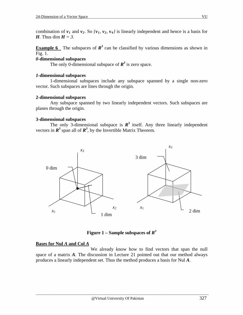
24-Dimension of a Vector Space VU
_______________________________________________________________________________________ @Virtual University Of Pakistan 327
combination of v1 and v2. So {v1, v2, v4} is linearly independent and hence is a basis for H. Thus dim H = 3. Example 6 The subspaces of R3 can be classified by various dimensions as shown in Fig. 1. 0-dimensional subspaces
The only 0-dimensional subspace of R3 is zero space. 1-dimensional subspaces
1-dimensional subspaces include any subspace spanned by a single non-zero vector. Such subspaces are lines through the origin. 2-dimensional subspaces
Any subspace spanned by two linearly independent vectors. Such subspaces are planes through the origin. 3-dimensional subspaces
The only 3-dimensional subspace is R3 itself. Any three linearly independent vectors in R3 span all of R3, by the Invertible Matrix Theorem.
Figure 1 – Sample subspaces of R3 Bases for Nul A and Col A We already know how to find vectors that span the null space of a matrix A. The discussion in Lecture 21 pointed out that our method always produces a linearly independent set. Thus the method produces a basis for Nul A.
x2
x3
x1 1 dim
0 dim
x3
x1 2 dim
3 dim

24-Dimension of a Vector Space VU
_______________________________________________________________________________________ @Virtual University Of Pakistan 328
Example 7 Find a basis for the null space of
2 2 -1 0 1-1 -1 2 -3 11 1 -2 0 -10 0 1 1 1
=
A .
Solution The null space of A is the solution space of homogeneous system 1 2 3 5
1 2 3 4 5
1 2 3 5
3 4 5
2x + 2x - x + x = 0- x - x + 2x - 3x + x = 0
x + x - 2x - x = 0x + x + x = 0
The most appropriate way to solve this system is to reduce its augmented matrix into reduced echelon form.
4 2 3 1
3 1 3 2
2 2 -1 0 1 0-1 -1 2 -3 1 0
, 1 1 -2 0 -1 0 0 0 1 1 1 0
1 1 -2 0 -1 0 0 0 1 1 1 0
2 , 3 2 2 -1 0 1 0-1 -1 2 -3 1 0
1 1 -2 0 -
R R R R
R R R R
− −
3 2
3
1 0 0 0 1 1 1 0
3 0 0 3 0 3 0-1 -1 2 -3 1 0
1 1 -2 0 -1 00 0 1 1 1 0 10 0 0 -3 0 0 3-1 -1 2 -3 1 0
1 1 -2 0 -1 00 0 1 1 1 00 0 0 1
R R
R
−
−
4 1 0 0-1 -1 2 -3 1 0
R R
+
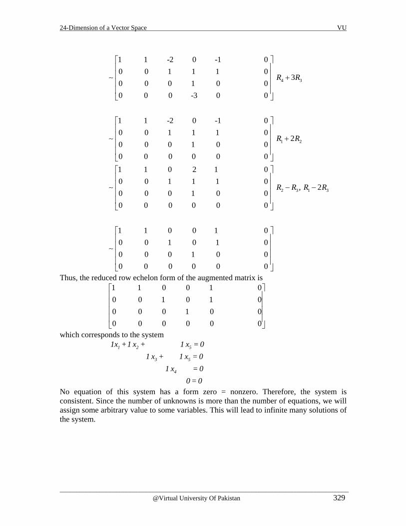
24-Dimension of a Vector Space VU
_______________________________________________________________________________________ @Virtual University Of Pakistan 329
4 3
1 2
1 1 -2 0 -1 00 0 1 1 1 0
30 0 0 1 0 00 0 0 -3 0 0
1 1 -2 0 -1 00 0 1 1 1 0
20 0 0 1 0 00 0 0 0 0 0
R R
R R
+
+
2 3 1 3
1 1 0 2 1 00 0 1 1 1 0
, 20 0 0 1 0 00 0 0 0 0 0
1 1 0 0 1 00 0 1 0 1 00 0 0 1 0 00 0 0 0 0 0
R R R R
− −
Thus, the reduced row echelon form of the augmented matrix is 1 1 0 0 1 00 0 1 0 1 00 0 0 1 0 00 0 0 0 0 0
which corresponds to the system 1 2 5
3 5
4
1x +1 x + 1 x = 01 x + 1 x = 0
1 x = 00 = 0
No equation of this system has a form zero = nonzero. Therefore, the system is consistent. Since the number of unknowns is more than the number of equations, we will assign some arbitrary value to some variables. This will lead to infinite many solutions of the system.

24-Dimension of a Vector Space VU
_______________________________________________________________________________________ @Virtual University Of Pakistan 330
1 2 5
2
3 5
4
5
x = - 1x -1xx = sx = - 1xx = 0x = t
The general solution of the given system is x1 = - s - t , x2 = s , x3 = - t , x4 = 0 , x5 = t
Therefore, the solution vector can be written as 1
2
3
4
5
x -s - t -s -t -1 -1x s s 0 1 0x = = + = s +t-t 0 -t 0 -1x 0 0 0 0 0x t 0 t 0 1
which shows that the vectors
-1 -11 00 and -10 00 1
= =
1 2v v span the solution space .Since they
are also linearly independent,{v1,v2} is a basis for Nul A. The next two examples describe a simple algorithm for finding a basis for the column space.
Example 8 Find a basis for Col B, where
1 4 0 2 00 0 1 -1 0
[ , ]0 0 0 0 10 0 0 0 0
= ..., =
1 2 5B b b b
Solution Each non-pivot column of B is a linear combination of the pivot columns. In fact, b2 = 4b1 and b4 = 2b1 – b3. By the Spanning Set Theorem, we may discard b2 and b4 and {b1, b3, b5} will still span Col B. Let
1 0 00 1 0
{ } , ,0 0 10 0 0
= , , =
1 3 5S b b b
Since b1 ≠ 0 and no vector in S is a linear combination of the vectors that precede it, S is linearly independent. Thus S is a basis for Col B. What about a matrix A that is not in reduced echelon form? Recall that any linear dependence relationship among the columns of A can be expressed in the form Ax

24-Dimension of a Vector Space VU
_______________________________________________________________________________________ @Virtual University Of Pakistan 331
= 0, where x is a column of weights. (If some columns are not involved in a particular dependence relation, then their weights are zero.) When A is row reduced to a matrix B, the columns of B are often totally different from the columns of A. However, the equations Ax = 0 and Bx = 0 have exactly the same set of solutions. That is, the columns of A have exactly the same linear dependence relationships as the columns of B. Elementary row operations on a matrix do not affect the linear dependence relations among the columns of the matrix. Example 9 It can be shown that the matrix
1 4 0 2 -13 12 1 5 5
[ ]2 8 1 3 25 20 2 8 8
= ... =
1 2 5A a a a
is row equivalent to the matrix B in Example 8. Find a basis for Col A. Solution In Example 8, we have seen that = 4 and = 2 -2 1 4 1 3b b b b b so we can expect that = 4 and = 2 -2 1 4 1 3a a a a a . This is indeed the case. Thus, we may discard a2 and a4 while selecting a minimal spanning set for Col A. In fact, {a1, a3, a5} must be linearly independent because any linear dependence relationship among a1, a3, a5 would imply a linear dependence relationship among b1, b3, b5. But we know that {b1, b3, b5} is a linearly independent set. Thus {a1, a3, a5} is a basis for Col A. The columns we have used for this basis are the pivot columns of A. Examples 8 and 9 illustrate the following useful fact. Theorem 3 The pivot columns of a matrix A form a basis for Col A. Proof The general proof uses the arguments discussed above. Let B be the reduced echelon form of A. The set of pivot columns of B is linearly independent, for no vector in the set is a linear combination of the vectors that precede it. Since A is row equivalent to B, the pivot columns of A are linearly independent too, because any linear dependence relation among the columns of A corresponds to a linear dependence relation among the columns of B. For this same reason, every non-pivot column of A is a linear combination of the pivot columns of A. Thus the non-pivot columns of A may be discarded from the spanning set for Col A, by the Spanning Set Theorem. This leaves the pivot columns of A as a basis for Col A. Note Be careful to use pivot columns of A itself for the basis of Col A. The columns of an echelon form B are often not in the column space of A. For instance, the columns of the B in Example 8 all have zeros in their last entries, so they cannot span the column space of the A in Example 9.
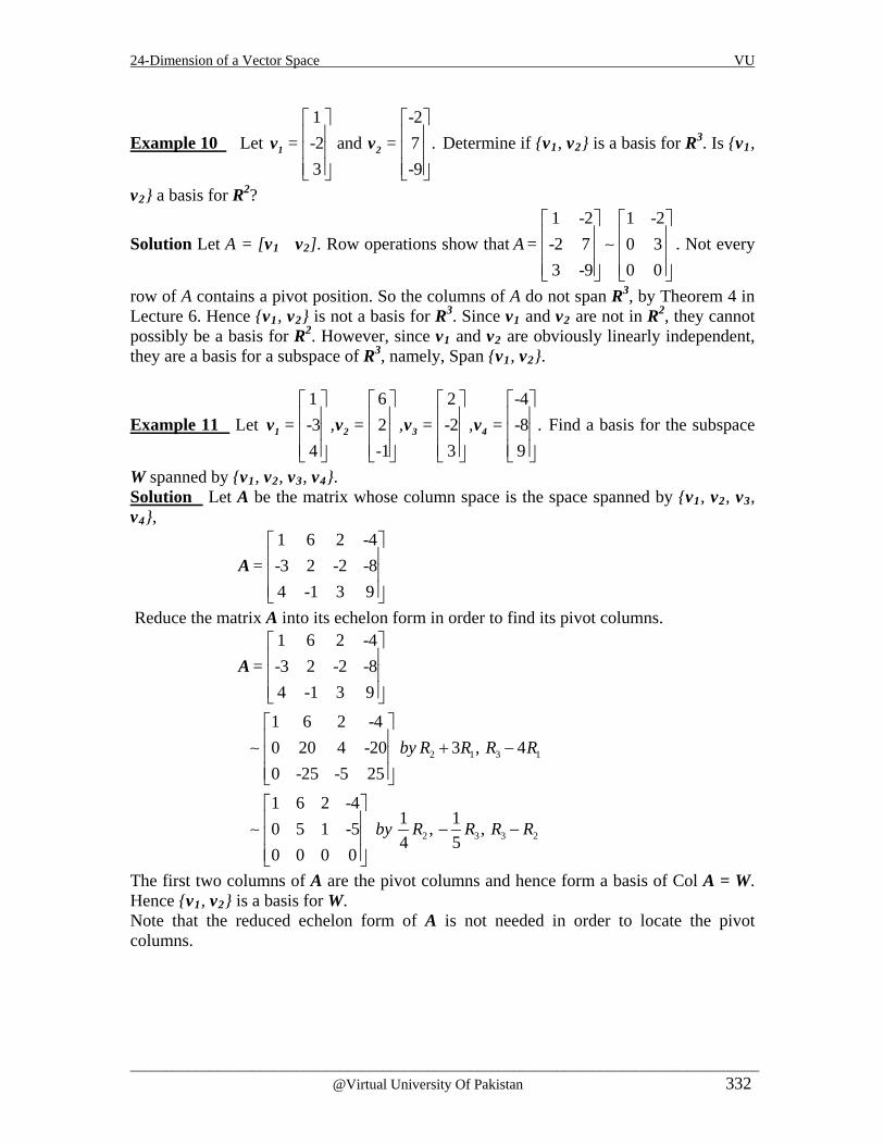
24-Dimension of a Vector Space VU
_______________________________________________________________________________________ @Virtual University Of Pakistan 332
Example 10 Let 1 -2-2 and 7 .3 -9
= =
1 2v v Determine if {v1, v2} is a basis for R3. Is {v1,
v2} a basis for R2?
Solution Let A = [v1 v2]. Row operations show that1 -2 1 -2-2 7 0 33 -9 0 0
A=
. Not every
row of A contains a pivot position. So the columns of A do not span R3, by Theorem 4 in Lecture 6. Hence {v1, v2} is not a basis for R3. Since v1 and v2 are not in R2, they cannot possibly be a basis for R2. However, since v1 and v2 are obviously linearly independent, they are a basis for a subspace of R3, namely, Span {v1, v2}.
Example 11 Let 1 6 2 -4-3 2 -2 -8 .4 -1 3 9
= , = , = , =
1 2 3 4v v v v Find a basis for the subspace
W spanned by {v1, v2, v3, v4}. Solution Let A be the matrix whose column space is the space spanned by {v1, v2, v3, v4},
1 6 2 -4-3 2 -2 -84 -1 3 9
=
A
Reduce the matrix A into its echelon form in order to find its pivot columns.
2 1 3 1
2 3 3 2
1 6 2 -4-3 2 -2 -84 -1 3 9
1 6 2 -40 20 4 -20 3 , 40 -25 -5 25
1 6 2 -41 10 5 1 -5 , ,4 5
0 0 0 0
=
by R R R R
by R R R R
+ − − −
A
The first two columns of A are the pivot columns and hence form a basis of Col A = W. Hence {v1, v2} is a basis for W. Note that the reduced echelon form of A is not needed in order to locate the pivot columns.

24-Dimension of a Vector Space VU
_______________________________________________________________________________________ @Virtual University Of Pakistan 333
Procedure Basis and Linear Combinations Given a set of vectors S = {v1, v2, …,vk} in Rn, the following procedure produces a subset of these vectors that form a basis for span (S) and expresses those vectors of S that are not in the basis as linear combinations of the basis vector. Step1: Form the matrix A having v1, v2,..., vk as its column vectors. Step2: Reduce the matrix A to its reduced row echelon form R, and let
w1, w2,…, wk be the column vectors of R. Step3: Identify the columns that contain the leading entries i.e., 1’s in R. The
corresponding column vectors of A are the basis vectors for span (S). Step4: Express each column vector of R that does not contain a leading entry as
a linear combination of preceding column vector that do contain leading entries (we will be able to do this by inspection). This yields a set of dependency equations involving the column vectors of R. The corresponding equations for the column vectors of A express the vectors which are not in the basis as linear combinations of basis vectors.
Example 12 Basis and Linear Combinations (a) Find a subset of the vectors v1 = (1, -2, 0, 3), v2 = (2, -4, 0, 6), v3 = (-1, 1, 2, 0) and v4 = (0, -1, 2, 3) that form a basis for the space spanned by these vectors. (b) Express each vector not in the basis as a linear combination of the basis vectors. Solution (a) We begin by constructing a matrix that has v1, v2, v3, v4 as its column vectors
1 2 -1 0-2 -4 1 -10 0 2 23 6 0 3
↑ ↑ ↑ ↑
1 2 3 4v v v v (A)
Finding a basis for column space of this matrix can solve the first part of our problem. Transforming Matrix to Reduced Row Echelon Form:
1 2 -1 0-2 -4 1 -1 0 0 2 2 3 6 0 3
1 2 -1 0 0 0 -1 -1 0 0 2 2 0 0 3 3
1 2
1 4
2 R + R-3R + R

24-Dimension of a Vector Space VU
_______________________________________________________________________________________ @Virtual University Of Pakistan 334
1 2 -1 0 0 0 1 1 0 0 2 2 0 0 3 3
2-1R
1 2 -1 0 0 0 1 1 0 0 0 0 0 0 0 0
2 3
2 4
-2R + R-3R + R
1 2 0 10 0 1 10 0 0 00 0 0 0
2 1R + R
Labeling the column vectors of the resulting matrix as w1, w2, w3 and w4 yields 1 2 0 10 0 1 10 0 0 00 0 0 0
↑↑ ↑ ↑
31 2 4ww w w
(B)
The leading entries occur in column 1 and 3 so {w1, w3} is a basis for the column space of (B) and consequently {v1, v3} is the basis for column space of (A). (b) We shall start by expressing w2 and w4 as linear combinations of the basis vector w1 and w3. The simplest way of doing this is to express w2 and w4 in term of basis vectors with smaller subscripts. Thus we shall express w2 as a linear combination of w1, and we shall express w4 as a linear combination of w1 and w3. By inspection of (B), these linear combinations are w2 = 2w1 and w4 = w1 + w3. We call them the dependency equations. The corresponding relationship of (A) are v3 = 2v1 and v5 = v1 + v3. Example 13 Basis and Linear Combinations (a) Find a subset of the vectors v1 = (1, -1, 5, 2), v2 = (-2, 3, 1, 0), v3 = (4, -5, 9, 4), v4 = (0, 4, 2, -3) and v5 = (-7, 18, 2, -8) that form a basis for the space spanned by these vectors. (b) Express each vector not in the basis as a linear combination of the basis vectors Solution (a) We begin by constructing a matrix that has v1, v2, ... , v5 as its column vectors

24-Dimension of a Vector Space VU
_______________________________________________________________________________________ @Virtual University Of Pakistan 335
1 -2 4 0 - 7 -1 3 -5 4 18 5 1 9 2 2 2 0 4 -3 -8
↑ ↑↑ ↑ ↑
3 51 2 4v vv v v
(A)
Finding a basis for column space of this matrix can solve the first part of our problem. Transforming Matrix to Reduced Row Echelon Form:
1 -2 4 0 - 7 -1 3 -5 4 18 5 1 9 2 2 2 0 4 -3 -8
1 - 2 4 0 - 7 0 1 -1 4 11 0 11 -11 2 37 0 4 - 4 -3 6
1 2
1 3
1 4
R + R-5R + R-2R + R
1 - 2 4 0 - 7 0 1 -1 4 11 0 0 0 - 42 -84 0 0 0 -19 -38
2 3
2 4
-11R + R-4R + R
1 - 2 4 0 - 7 0 1 -1 4 11 0 0 0 1 2 0 0 0 -19 -38
3(-1/42)R
1 - 2 4 0 - 7 0 1 -1 4 11 0 0 0 1 2 0 0 0 0 0
3 419R + R
1 - 2 4 0 - 7 0 1 -1 0 3 0 0 0 1 2 0 0 0 0 0
3 2(-4)R + R
1 0 2 0 -1 0 1 -1 0 3 0 0 0 1 2 0 0 0 0 0
2 12R + R

24-Dimension of a Vector Space VU
_______________________________________________________________________________________ @Virtual University Of Pakistan 336
Denoting the column vectors of the resulting matrix by w1 , w2 , w3, w4, and w5 yields 1 0 2 0 -1 0 1 -1 0 3 0 0 0 1 2 0 0 0 0 0
↑ ↑↑ ↑ ↑
3 51 2 4w ww w w
(B)
The leading entries occur in columns 1,2 and 4 so that {w1, w2, w4} is a basis for the column space of (B) and consequently {v1, v2, v4} is the basis for column space of (A). (b) We shall start by expressing w3 and w5 as linear combinations of the basis vector w1, w2, w4. The simplest way of doing this is to express w3 and w5 in term of basis vectors with smaller subscripts. Thus we shall express w3 as a linear combination of w1 and w2, and we shall express w5 as a linear combination of w1, w2, and w4. By inspection of (B), these linear combination are w3 = 2w1 – w2 and w5 = -w1 + 3w2 + 2w4. The corresponding relationship of (A) are v3 = 2v1 – v2 and v5 = -v1 + 3v2 + 2v4. Example 14 Basis and Linear Combinations (a) Find a subset of the vectors v1 = (1, -2, 0, 3), v2 = (2, -5, -3, 6), v3 = (0, 1, 3, 0), v4 = (2, -1, 4, -7) and v5 = (5 , -8, 1, 2) that form a basis for the space spanned by these vectors. (b) Express each vector not in the basis as a linear combination of the basis vectors. Solution (a) We begin by constructing a matrix that has v1, v2, ... , v5 as its column vectors
1 2 0 2 5-2 -5 1 -1 -80 -3 3 4 13 6 0 -7 2
↑ ↑ ↑ ↑ ↑
1 2 3 4 5v v v v v (A)
Finding a basis for column space of this matrix can solve the first part of our problem. Reducing the matrix to reduced-row echelon form and denoting the column vectors of the resulting matrix by w1, w2, w3, w4, and w5 yields
1 0 2 0 1 0 1 -1 0 1 0 0 0 1 1 0 0 0 0 0
↑ ↑↑ ↑ ↑
3 51 2 4w ww w w
(B)
The leading entries occur in columns 1, 2 and 4 so {w1, w2, w4} is a basis for the column space of (B) and consequently {v1, v2, v4} is the basis for column space of (A).

24-Dimension of a Vector Space VU
_______________________________________________________________________________________ @Virtual University Of Pakistan 337
(b) Dependency equations are w3 = 2w1 – w2 and w5 = w1 + w2 + w4 The corresponding relationship of (A) are v3 = 2v1 – v2 and v5 = v1 + v2 + v4 Subspaces of a Finite-Dimensional Space The next theorem is a natural counterpart to the Spanning Set Theorem. Theorem 5 Let H be a subspace of a finite-dimensional vector space V. Any linearly independent set in H can be expanded, if necessary, to a basis for H. Also, H is finite-dimensional and dim dim≤H V . When the dimension of a vector space or subspace is known, the search for a basis is simplified by the next theorem. It says that if a set has the right number of elements, then one has only to show either that the set is linearly independent or that it spans the space. The theorem is of critical importance in numerous applied problems (involving differential equations or difference equations, for example) where linear independence is much easier to verify than spanning. Theorem 5 (The Basis Theorem) Let V be a p-dimensional vector space, p> 1. Any linearly independent set of exactly p elements in V is automatically a basis for V. Any set of exactly p elements that spans V is automatically a basis for V. The Dimensions of Nul A and Col A Since the pivot columns of a matrix A form a basis for Col A, we know the dimension of Col A as soon as we know the pivot columns. The dimension of Nul A might seem to require more work, since finding a basis for Nul A usually takes more time than a basis for Col A. Yet, there is a shortcut. Let A be an m n× matrix, and suppose that the equation Ax = 0 has k free variables. From lecture 21, we know that the standard method of finding a spanning set for Nul A will produce exactly k linearly independent vectors say, u1, … , uk, one for each free variable. So {u1, … , uk} is a basis for Nul A, and the number of free variables determines the size of the basis. Let us summarize these facts for future reference. The dimension of Nul A is the number of free variables in the equation Ax = 0, and the dimension of Col A is the number of pivot columns in A. Example 15 Find the dimensions of the null space and column space of
-3 6 -1 1 -71 -2 2 3 -12 -4 5 8 -4
=
A
Solution Row reduce the augmented matrix [A 0] to echelon form and obtain 1 -2 2 3 -1 00 0 1 2 -2 00 0 0 0 0 0

24-Dimension of a Vector Space VU
_______________________________________________________________________________________ @Virtual University Of Pakistan 338
Writing it in equations form, we get 1 2 3 4 5
3 4 5
2 2 3 02 2 0
x x x x xx x x− + + − =+ − =
Since the number of unknowns is more than the number of equations, we will introduce free variables here (say) x2, x4 and x5. Hence the dimension of Nul A is 3. Also dim Col A is 2 because A has two pivot columns. Example 16 Decide whether each statement is true or false, and give a reason for each answer. Here V is a non-zero finite-dimensional vector space.
1. If dim V = p and if S is a linearly dependent subset of V, then S contains more than p vectors. 2. If S spans V and if T is a subset of V that contains more vectors than S, then T is linearly dependent.
Solution 1. False. Consider the set {0}. 2. True. By the Spanning Set Theorem, S contains a basis for V; call that basis ′S .
Then T will contain more vectors than ′S . By Theorem 1, T is linearly dependent.

24-Dimension of a Vector Space VU
_______________________________________________________________________________________ @Virtual University Of Pakistan 339
Exercises For each subspace in exercises 1-6, (a) find a basis and (b) state the dimension.
1. 2
: , in3
s ts t s tt
− +
R 2.
2
: , , in32
ca b
a b cb ca b
− − +
R
3.
4 22 5 4
: , , in2
3 7 6
a b ca b c
a b ca ca b c
− − + − − + − + +
R 4.
3 66 2 2
: , , in9 5 33
a b ca b c
a b ca b ca b c
+ − − − − + + − + +
R
5. {(a, b, c): a – 3b + c = 0, b – 2c = 0, 2b – c = 0} 6 {(a, b, c, d): a - 3b + c = 0} 7. Find the dimension of the subspace H of R2 spanned by
2 4 3, ,
5 10 6− −
−
8. Find the dimension of the subspace spanned by the given vectors.
1 3 9 70 , 1 , 4 , 32 1 2 1
− − −
Determine the dimensions of Nul A and Col A for the matrices shown in exercises 9 to 12.
9.
1 6 9 0 20 1 2 4 50 0 0 5 10 0 0 0 0
− − − =
A 10.
1 3 4 2 1 60 0 1 3 7 00 0 0 1 4 30 0 0 0 0 0
− − − = −
A
11. 1 0 9 50 0 1 4
= − A 12.
1 1 00 4 70 0 5
− =
A

24-Dimension of a Vector Space VU
_______________________________________________________________________________________ @Virtual University Of Pakistan 340
13. The first four Hermite polynomials are 1, 2t, -2 + 4t2, and -12t + 8t3. These polynomials arise naturally in the study of certain important differential equations in mathematical physics. Show that the first four Hermite polynomials form a basis of P3. 14. Let B be the basis of P3 consisting of the Hermite polynomials in exercise 13, and let p (t) = 7 – 12 t – 8 t2 + 12 t3. Find the coordinate vector of p relative to B. 15. Extend the following vectors to a basis for R5:
9 9 67 4 7
8 , 1 , 85 6 5
7 7 7
− − = = = − − − −
1 2 3v v v

25- Rank VU
©Virtual University Of Pakistan 341
Lecture 25
Rank
With the help of vector space concepts, for a matrix several interesting and useful relationships in matrix rows and columns have been discussed. For instance, imagine placing 2000 random numbers into a 40 x 50 matrix A and then determining both the maximum number of linearly independent columns in A and the maximum number of linearly independent columns in AT (rows in A). Remarkably, the two numbers are the same. Their common value is called the rank of the matrix. To explain why, we need to examine the subspace spanned by the subspace spanned by the rows of A. The Row Space If A is an m n× matrix, each row of A has n entries and thus can be identified with a vector in Rn. The set of all linear combinations of the row vectors is called the row space of A and is denoted by Row A. Each row has n entries, so Row A is a subspace of Rn. Since the rows of A are identified with the columns of AT, we could also write Col AT in place of Row A.
Example 1 Let
-2 -5 8 0 -171 3 -5 1 5
and3 11 -19 7 11 7 -13 5 -3
= (-2,-5,8,0,-17)= (1,3,-5,1,5)
== (3,11,-19,7,1)= (1,7,-13,5,-3)
1
2
3
4
rr
Arr
The row space of A is the subspace of R5 spanned by {r1, r2, r3, r4}. That is, Row A = Span {r1, r2, r3, r4}. Naturally, we write row vectors horizontally; however, they could also be written as column vectors Example Let
That is Row A=Span {r1, r2}. We could use the Spanning Set Theorem to shrink the spanning set to a basis. Some times row operation on a matrix will not give us the required information but row reducing certainly worthwhile, as the next theorem shows Theorem 1 If two matrices A and B are row equivalent, then their row spaces are the same. If B is in echelon form, the nonzero rows of B form a basis for the row space of A as well as B. Theorem 2 If A and B are row equivalent matrices, then
2 1 0and
3 -1 4
= (2,1,0)= (3,-1,4)
=
1
2
rr
A

25- Rank VU
©Virtual University Of Pakistan 342
(a) A given set of column vectors of A is linearly independent if and only if the corresponding column vectors of B are linearly independent. (b) A given set of column vector of A forms a basis for the column space of A if and only if the corresponding column vector of B forms a basis for the column space of B. Example 2 (Bases for Row and Column Spaces)
Find the bases for the row and column spaces of
1 -3 4 -2 5 42 -6 9 -1 8 22 -6 9 -1 9 7-1 3 -4 2 -5 -4
=
A .
Solution We can find a basis for the row space of A by finding a basis for the row space of any row-echelon form of A.
Now
1 -3 4 - 2 5 4 2 - 6 9 -1 8 2 2 - 6 9 -1 9 7-1 3 -4 2 -5 - 4
1 -3 4 - 2 5 4 0 0 1 3 - 2 - 6 0 0 1 3 -1 -1 0 0 0 0 0 0
1 2
1 3
1 4
-2 R + R-2 R + R
R + R
1 -3 4 - 2 5 4 0 0 1 3 - 2 - 6 0 0 0 0 1 5 0 0 0 0 0 0
2 3-1R + R
Row-echelon form of A:
1 -3 4 -2 5 40 0 1 3 -2 -60 0 0 0 1 50 0 0 0 0 0
=
R
Here Theorem 1 implies that that the non zero rows are the basis vectors of the matrix. So these bases vectors are
[ ][ ][ ]
1 -3 4 -2 5 4
0 0 1 3 -2 -6
0 0 0 0 1 5
=
=
=
1
2
3
r
r
r
A and R may have different column spaces, we cannot find a basis for the column space of A directly from the column vectors of R. however, it follows from the theorem (2b) if

25- Rank VU
©Virtual University Of Pakistan 343
we can find a set of column vectors of R that forms a basis for the column space of R, then the corresponding column vectors of A will form a basis for the column space of A. The first, third, and fifth columns of R contains the leading 1’s of the row vectors, so
1 4 50 1 -20 0 10 0 0
1 = = =
′ ′ ′
3 5c c c
form a basis for the column space of R, thus the corresponding column vectors of A
namely,
1 4 52 9 82 9 9-1 -4 -5
= = =
1 3 5c c c
form a basis for the column space of A. Example The matrix
is in row-echelon form. The vectors
form a basis for the row space of R, and the vectors 1 -2 00 1 0
, ,0 0 10 0 0
c = c = c =
1 2 3
form a basis for the column space of R.
1 -2 5 0 30 1 3 0 00 0 0 1 00 0 0 0 0
R =
[ ][ ][ ]
1 -2 5 0 3
0 1 3 0 0
0 0 0 1 0
=
=
=
1
2
3
r
r
r

25- Rank VU
©Virtual University Of Pakistan 344
Example 3 (Basis for a Vector Space using Row Operation) Find bases for the space spanned by the vectors
= (1,-2,0,0,3) = (2,-5,-3,-2,6)= (0,5,15,10,0) = (2,6,18,8,6)
1 2
3 4
v vv v
Solution The space spanned by these vectors is the row space of the matrix
1 -2 0 0 32 -5 -3 -2 60 5 15 10 02 6 18 8 6
Transforming Matrix to Row Echelon Form:
1 - 2 0 0 32 -5 -3 - 2 60 5 15 10 02 6 18 8 6
1 - 2 0 0 3 0 1 3 2 0 0 5 15 10 0 0 10 18 8 0
1 2
1 4
2
(-2)R + R(-2)R + R
(-1)R
1 - 2 0 0 3 0 1 3 2 0 0 0 0 0 0 0 0 -12 -12 0
2 3
2 4
(-5)R + R(-10)R + R
1 - 2 0 0 3 0 1 3 2 0 0 0 -12 -12 0 0 0 0 0 0
34R
1 - 2 0 0 3 0 1 3 2 0 0 0 1 1 0 0 0 0 0 0
3(-1/12)R

25- Rank VU
©Virtual University Of Pakistan 345
Therefore,
1 -2 0 0 30 1 3 2 00 0 1 1 00 0 0 0 0
=
R
The non-zero row vectors in this matrix are = (1,-2,0,0,3), = (0,1,3,2,0), = (0,0,1,1,0)1 2 3w w w
These vectors form a basis for the row space and consequently form a basis for the subspace of R5 spanned by v1, v2, v3. Example 4 (Basis for the Row Space of a Matrix)
Find a basis for the row space of
1 -2 0 0 32 -5 -3 -2 60 5 15 10 02 6 18 8 6
=
A consisting entirely of row
vectors from A. Solution We find AT; then we will use the method of example (2) to find a basis for the column space of AT; and then we will transpose again to convert column vectors back to row vectors. Transposing A yields
1 2 0 2-2 -5 5 60 -3 15 180 -2 10 83 6 0 6
=
TA
Transforming Matrix to Row Echelon Form: 1 2 0 2-2 -5 5 6 0 -3 15 18 0 - 2 10 8 3 6 0 6
1 2 0 2 0 -1 5 10 0 -3 15 18 0 - 2 10 8 0 0 0 0
1 2
1 5
2 R + R(-3)R + R

25- Rank VU
©Virtual University Of Pakistan 346
1 2 0 2 0 1 -5 -10 0 -3 15 18 0 - 2 10 8 0 0 0 0
2(-1)R
1 2 0 2 0 1 -5 -10 0 0 0 -12 0 0 0 -12 0 0 0 0
2 3
2 4
(3)R + R(2)R + R
1 2 0 2 0 1 -5 -10 0 0 0 1 0 0 0 -12 0 0 0 0
3(-1/12)R
1 2 0 2 0 1 -5 -10 0 0 0 1 0 0 0 0 0 0 0 0
3 412 R + R
Now
1 2 0 20 1 -5 -100 0 0 10 0 0 00 0 0 0
=
R
The first, second and fourth columns contain the leading 1’s, so the corresponding column vectors in AT form a basis for the column space of AT; these are
1 2 2-2 -5 6
and0 -3 180 -2 83 6 6
= , = =
1 2 4c c c
Transposing again and adjusting the notation appropriately yields the basis vectors [ ] [ ] [ ]1 -2 0 0 3 2 -5 -3 -2 6 2 6 18 8 6= , = and =1 2 4r r r
for the row space of A.

25- Rank VU
©Virtual University Of Pakistan 347
The following example shows how one sequence of row operations on A leads to bases for the three spaces: Row A, Col A, and Nul A. Example 5 Find bases for the row space, the column space and the null space of the matrix
Solution To find bases for the row space and the column space, row reduce A to an
echelon form:
1 3 -5 1 50 1 -2 2 -70 0 0 -4 200 0 0 0 0
=
A B
By Theorem (1), the first three rows of B form a basis for the row space of A (as well as the row space of B). Thus Basis for Row A:
{(1, 3, -5, 1, 5), (0, 1, -2, 2, -7), (0, 0, 0, -4, 20)} For the column space, observe from B that the pivots are in columns 1, 2 and 4. Hence columns 1, 2 and 4 of A (not B) form a basis for Col A:
-2 -5 01 3 1
Basis for Col : , ,3 11 71 7 5
A
Any echelon form of A provides (in its nonzero rows) a basis for Row A and also identifies the pivot columns of A for Col A. However, for Nul A, we need the reduced echelon form. Further row operations on B yield
1 0 1 0 10 1 -2 0 30 0 0 1 -50 0 0 0 0
=
A B C
The equation Ax = 0 is equivalent to Cx = 0, that is, 1 3 5
2 3 5
4 5
x + x + x = 0 x - 2x + 3x = 0 x - 5x = 0
-2 -5 8 0 -171 3 -5 1 53 11 -19 7 11 7 -13 5 -3
=
A

25- Rank VU
©Virtual University Of Pakistan 348
So x1 = -x3 – x5, x2 = 2x3 – 3x5, x4 = 5x5, with x3 and x5 free variables. The usual calculations (discussed in lecture 21) show that
-1 -12 -3
Basis for Nul : ,1 00 50 1
A
Observe that, unlike the bases for Col A, the bases for Row A and Nul A have no simple connection with the entries in A itself. Note 1. Although the first three rows of B in Example (5) are linearly independent, it is wrong
to conclude that the first three rows of A are linearly independent. (In fact, the third row of A is 2 times the first row plus 7 times the second row).
2. Row operations do not preserve the linear dependence relations among the rows of a matrix.
Definition The rank of A is the dimension of the column space of A. Since Row A is the same as Col AT, the dimension of the row space of A is the rank of AT. The dimension of the null space is sometimes called the nullity of A. Theorem 3 (The Rank Theorem) The dimensions of the column space and the row space of an m n× matrix A are equal. This common dimension, the rank of A, also equals the number of pivot positions in A and satisfies the equation
rank A + dim Nul A = n Example 6 (a) If A is a 7 9× matrix with a two – dimensional null space, what is the rank of A? (b). Could a 6 9× matrix have a two – dimensional null space? Solution (a) Since A has 9 columns, (rank A) + 2 = 9 and hence rank A = 7. (b) No, If a 6 9× matrix, call it B, had a two – dimensional null space, it would have to have rank 7, by the Rank Theorem. But the columns of B are vectors in R6 and so the dimension of Col B cannot exceed 6; that is, rank B cannot exceed 6. The next example provides a nice way to visualize the subspaces we have been studying. Later on, we will learn that Row A and Nul A have only the zero vector in common and are actually “perpendicular” to each other. The same fact will apply to Row AT (= Col A) and Nul AT. So the figure in Example (7) creates a good mental image for the general case.

25- Rank VU
©Virtual University Of Pakistan 349
Example 7 Let 3 0 13 0 14 0 5
− = −
A . It is readily checked that Nul A is the x2 – axis, Row
A is the x1x3 – plane, Col A is the plane whose equation is x1 – x2 = 0 and Nul AT is the set of all multiples of (1, -1, 0). Figure 1 shows Nul A and Row A in the domain of the linear transformation ;→x Ax the range of this mapping, Col A, is shown in a separate copy of R3, along with Nul AT.
Figure 1 – Subspaces associated with a matrix A
Applications to Systems of Equations The Rank Theorem is a powerful tool for processing information about systems of linear equations. The next example simulates the way a real-life problem using linear equations might be stated, without explicit mention of linear algebra terms such as matrix, subspace and dimension. Example 8 A scientist has found two solutions to a homogeneous system of 40 equations in 42 variables. The two solutions are not multiples and all other solutions can be constructed by adding together appropriate multiples of these two solutions. Can the scientist be certain that an associated non-homogeneous system (with the same coefficients) has a solution? Solution Yes. Let A be the 40 42× coefficient matrix of the system. The given information implies that the two solutions are linearly independent and span Nul A. So dim Nul A = 2. By the Rank Theorem, dim Col A = 42 – 2 = 40. Since R40 is the only subspace of R40 whose dimension is 40, Col A must be all of R40. This means that every non-homogeneous equation Ax = b has a solution.
x2 x1
x3
0
Row A
Nul A x2
x1
0
Col A
Nul AT
x3
R3 R3

25- Rank VU
©Virtual University Of Pakistan 350
Example 9 Find the rank and nullity of the matrix
-1 2 0 4 5 -33 -7 2 0 1 42 -5 2 4 6 14 -9 2 -4 -4 7
=
A .
Verify that values obtained verify the dimension theorem.
Solution
-1 2 0 4 5 -3 3 - 7 2 0 1 4 2 -5 2 4 6 1 4 -9 2 - 4 - 4 7
1 - 2 0 - 4 -5 3 3 - 7 2 0 1 4 2 -5 2 4 6 1 4 -9 2 - 4 - 4 7
1(-1)R
1 - 2 0 - 4 -5 3 0 -1 2 12 16 -5 0 -1 2 12 16 -5 0 -1 2 12 16 -5
1 2
1 3
1 4
(-3)R + R(-2)R + R(-4)R + R
1 - 2 0 - 4 -5 3 0 1 - 2 -12 -16 5 0 -1 2 12 16 -5 0 -1 2 12 16 -5
2(-1)R
1 - 2 0 - 4 -5 3 0 1 - 2 -12 -16 5 0 0 0 0 0 0 0 0 0 0 0 0
2 3
2 4
R + RR + R
1 0 - 4 - 28 -37 13 0 1 - 2 -12 -16 5 0 0 0 0 0 0 0 0 0 0 0 0
2 12R + R
The reduced row-echelon form of A is 1 0 -4 -28 -37 130 1 -2 -12 -16 50 0 0 0 0 00 0 0 0 0 0
(1)

25- Rank VU
©Virtual University Of Pakistan 351
The corresponding system of equations will be 1 3 4 5 6
2 3 4 5 6
x - 4x - 28x - 37x + 13x = 0x - 2x -12x - 16x + 5x = 0
or, on solving for the leading variables, 1 3 4 5 6
2 3 4 5 6
x = 4x - 28x + 37x - 13xx = 2x +12x + 16x - 5x (2)
it follows that the general solution of the system is 1
2
3
4
5
6
x = 4r + 28s + 37t - 13ux = 2r + 12s + 16t - 5ux = rx = sx = tx = u
or equivalently,
1
2
3
4
5
6
x 4 28 37 -13x 2 12 16 -5x 1 0 0 0
= r + s +t +ux 0 1 0 0x 0 0 1 0x 0 0 0 1
(3)
The four vectors on the right side of (3) form a basis for the solution space, so
nullity (A) = 4. The matrix
-1 2 0 4 5 -33 -7 2 0 1 42 -5 2 4 6 14 -9 2 -4 -4 7
=
A has 6 columns,
so rank(A) + nullity(A) = 2 + 4 = 6 = n

25- Rank VU
©Virtual University Of Pakistan 352
Example 10 Find the rank and nullity of the matrix; then verify that the values
obtained satisfy the dimension theorem
1 -3 2 2 10 3 6 0 -32 -3 -2 4 43 -6 0 6 5-2 9 2 -4 -5
=
A
Solution Transforming Matrix to the Reduced Row Echelon Form: 1 -3 2 2 1 0 3 6 0 -3 2 -3 - 2 4 4 3 - 6 0 6 5 - 2 9 2 - 4 -5
1 -3 2 2 1 0 3 6 0 -3 0 3 - 6 0 2 0 3 - 6 0 2 0 3 6 0 -3
1 3
1 4
1 5
(-2)R + R(-3)R + R
2R + R
1 -3 2 2 1 0 1 2 0 -1 0 3 - 6 0 2 0 3 - 6 0 2 0 3 6 0 -3
2(1/3)R
1 -3 2 2 1 0 1 2 0 -1 0 0 -12 0 5 0 0 -12 0 5 0 0 0 0 0
2 3
2 4
2 5
(-3) R + R(-3) R + R(-3)R + R
1 -3 2 2 1 0 1 2 0 -1 0 0 1 0 -5/12 0 0 -12 0 5 0 0 0 0 0
3(-1/12)R
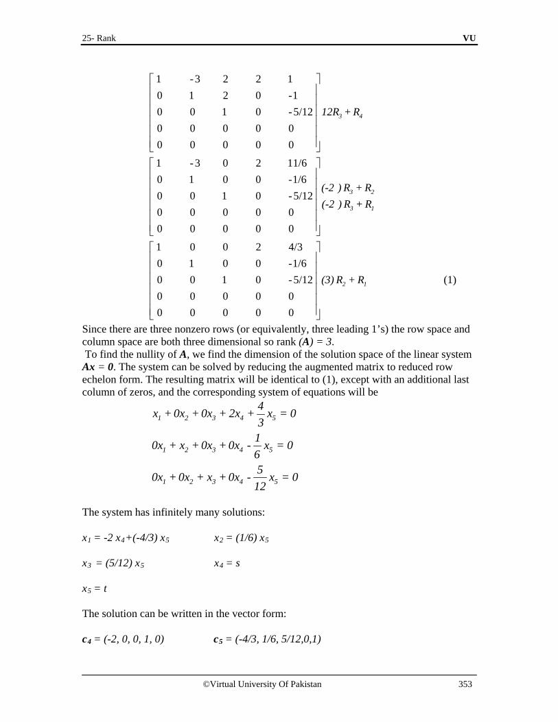
25- Rank VU
©Virtual University Of Pakistan 353
1 -3 2 2 1 0 1 2 0 -1 0 0 1 0 -5/12 0 0 0 0 0 0 0 0 0 0
3 412R + R
1 -3 0 2 11/6 0 1 0 0 -1/6 0 0 1 0 -5/12 0 0 0 0 0 0 0 0 0 0
3 2
3 1
(-2 ) R + R(-2 ) R + R
1 0 0 2 4/3 0 1 0 0 -1/6 0 0 1 0 -5/12 0 0 0 0 0 0 0 0 0 0
2 1(3) R + R
(1)
Since there are three nonzero rows (or equivalently, three leading 1’s) the row space and column space are both three dimensional so rank (A) = 3. To find the nullity of A, we find the dimension of the solution space of the linear system Ax = 0. The system can be solved by reducing the augmented matrix to reduced row echelon form. The resulting matrix will be identical to (1), except with an additional last column of zeros, and the corresponding system of equations will be
1 2 3 4 5
1 2 3 4 5
1 2 3 4 5
4x + 0x + 0x + 2x + x = 03
10x + x + 0x + 0x - x = 0650x + 0x + x + 0x - x = 0
12
The system has infinitely many solutions:
x1 = -2 x4+(-4/3) x5 x2 = (1/6) x5
x3 = (5/12) x5 x4 = s
x5 = t
The solution can be written in the vector form:
c4 = (-2, 0, 0, 1, 0) c5 = (-4/3, 1/6, 5/12,0,1)
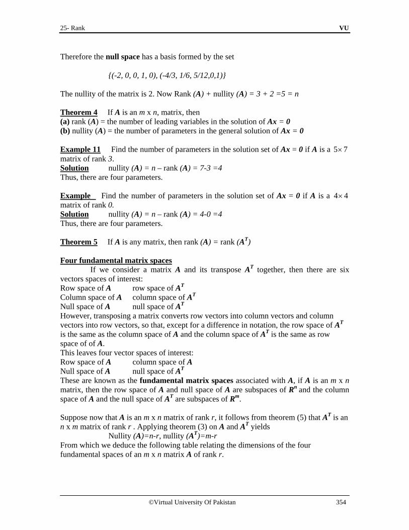
25- Rank VU
©Virtual University Of Pakistan 354
Therefore the null space has a basis formed by the set
{(-2, 0, 0, 1, 0), (-4/3, 1/6, 5/12,0,1)}
The nullity of the matrix is 2. Now Rank (A) + nullity (A) = 3 + 2 =5 = n Theorem 4 If A is an m x n, matrix, then (a) rank (A) = the number of leading variables in the solution of Ax = 0 (b) nullity (A) = the number of parameters in the general solution of Ax = 0 Example 11 Find the number of parameters in the solution set of Ax = 0 if A is a 5 7× matrix of rank 3. Solution nullity (A) = n – rank (A) = 7-3 =4 Thus, there are four parameters. Example Find the number of parameters in the solution set of Ax = 0 if A is a 4 4× matrix of rank 0. Solution nullity (A) = n – rank (A) = 4-0 =4 Thus, there are four parameters. Theorem 5 If A is any matrix, then rank (A) = rank (AT) Four fundamental matrix spaces
If we consider a matrix A and its transpose AT together, then there are six vectors spaces of interest: Row space of A row space of AT
Column space of A column space of AT
Null space of A null space of AT
However, transposing a matrix converts row vectors into column vectors and column vectors into row vectors, so that, except for a difference in notation, the row space of AT is the same as the column space of A and the column space of AT is the same as row space of of A. This leaves four vector spaces of interest: Row space of A column space of A Null space of A null space of AT These are known as the fundamental matrix spaces associated with A, if A is an m x n matrix, then the row space of A and null space of A are subspaces of Rn and the column space of A and the null space of AT are subspaces of Rm. Suppose now that A is an m x n matrix of rank r, it follows from theorem (5) that AT is an n x m matrix of rank r . Applying theorem (3) on A and AT yields
Nullity (A)=n-r, nullity (AT)=m-r From which we deduce the following table relating the dimensions of the four fundamental spaces of an m x n matrix A of rank r.

25- Rank VU
©Virtual University Of Pakistan 355
Fundamental space Dimension Row space of A r Column space of A r Null space of A n-r Null space of AT m-r Example 12 If A is a 7 x 4 matrix, then the rank of A is at most 4 and, consequently, the seven row vectors must be linearly dependent. If A is a 4 x 7 matrix, then again the rank of A is at most 4 and, consequently, the seven column vectors must be linearly dependent. Rank and the Invertible Matrix Theorem The various vector space concepts associated with a matrix provide several more statements for the Invertible Matrix Theorem. We list only the new statements here, but we reference them so they follow the statements in the original Invertible Matrix Theorem in lecture 13. Theorem 6 The Invertible Matrix Theorem (Continued) Let A be an n x n matrix. Then the following statements are each equivalent to the statement that A is an invertible matrix.
m. The columns of A form a basis of Rn. n. Col A = Rn. o. dim Col A = n p. rank A = n q. Nul A = {0} r. dim Nul A = 0
Proof Statement (m) is logically equivalent to statements (e) and (h) regarding linear independence and spanning. The other statements above are linked into the theorem by the following chain of almost trivial implications:
( ) ( ) ( ) ( ) ( ) ( ) ( )g n o p r q d⇒ ⇒ ⇒ ⇒ ⇒ ⇒ Only the implication (p) ⇒ (r) bears comment. It follows from the Rank Theorem because A is n n× . Statements (d) and (g) are already known to be equivalent, so the chain is a circle of implications. We have refrained from adding to the Invertible Matrix Theorem obvious statements about the row space of A, because the row space is the column space of AT. Recall from (1) of the Invertible Matrix Theorem that A is invertible if and only if AT is invertible. Hence every statement in the Invertible Matrix Theorem can also be stated for AT. Numerical Note Many algorithms discussed in these lectures are useful for understanding concepts and making simple computations by hand. However, the algorithms are often unsuitable for large-scale problems in real life. Rank determination is a good example. It would seem easy to reduce a matrix to echelon form and count the pivots. But unless exact arithmetic is performed on a matrix whose entries are specified exactly, row operations can change the apparent rank of a matrix.

25- Rank VU
©Virtual University Of Pakistan 356
For instance, if the value of x in the matrix 5 75 x
is not stored exactly as 7 in a
computer, then the rank may be 1 or 2, depending on whether the computer treats x – 7 as zero. In practical applications, the effective rank of a matrix A is often determined from the singular value decomposition of A. Example 13 The matrices below are row equivalent
2 -1 1 -6 8 1 -2 -4 3 -21 -2 -4 3 -2 0 3 9 -12 12-7 8 10 3 -10 0 0 0 0 04 -5 -7 0 4 0 0 0 0 0
= , =
A B
1. Find rank A and dim Nul A. 2. Find bases for Col A and Row A. 3. What is the next step to perform if one wants to find a basis for Nul A? 4. How many pivot columns are in a row echelon form of AT?
Solution 1. A has two pivot columns, so rank A = 2. Since A has 5 columns altogether, dim
Nul A = 5 – 2 = 3. 2. The pivot columns of A are the first two columns. So a basis for Col A is
2 -11 -2
,-7 84 -5
{ , }=
1 2a a
The nonzero rows of B form a basis for Row A, namely {(1, –2, –4, 3, –2), (0, 3, 9, –12, 12)}. In this particular example, it happens that any two rows of A form a basis for the row space, because the row space is two-dimensional and none of the rows of A is a multiple of another row. In general, the nonzero rows of an echelon form of A should be used as a basis for Row A, not the rows of A itself.
3. For Nul A, the next step is to perform row operations on B to obtain the reduced echelon form of A.
4. Rank AT = rank A, by the Rank Theorem, because Col AT = Row A. So AT has two pivot positions.
Exercises In exercises 1 to 4, assume that the matrix A is row equivalent to B. Without calculations, list rank A and dim Nul A. Then find bases for Col A, Row A, and Nul A.
1. 1 4 9 7 1 0 1 51 2 4 1 , 0 2 5 6
5 6 10 7 0 0 0 0
− − − = − − = − − −
A B

25- Rank VU
©Virtual University Of Pakistan 357
2.
1 3 4 1 9 1 3 0 5 72 6 6 1 10 0 0 2 3 8
,3 9 6 6 3 0 0 0 0 5
3 9 4 9 0 0 0 0 0 0
− − − − − − − − − = − − − − −
A B =
3.
2 3 6 2 5 2 3 6 2 52 3 3 3 4 0 0 3 1 1
,4 6 9 5 9 0 0 0 1 32 3 3 4 1 0 0 0 0 0
− − − − − − − = = − − −
A B
4.
1 1 3 7 9 9 1 1 3 7 9 91 2 4 10 13 12 0 1 1 3 4 3
,1 1 1 1 1 3 0 0 0 1 1 21 3 1 5 7 3 0 0 0 0 0 01 2 0 0 5 4 0 0 0 0 0 0
− − − − − − − − = =− − − − − − − − − − −
A B
5. If a 3 x 8 matrix A has rank 3, find dim Nul A, dim Row A, and rank AT. 6. If a 6 x 3 matrix A has rank 3, find dim Nul A, dim Row A, and rank AT. 7. Suppose that a 4 x 7 matrix A has four pivot columns. Is Col A = R4? Is Nul A = R3? Explain your answers. 8. Suppose that a 5 x 6 matrix A has four pivot columns. What is dim Nul A? Is Col A = R4? Why or why not? 9. If the null space of a 5 x 6 matrix A is 4-dimensional, what is the dimension of the column space of A? 10. If the null space of a 7 x 6 matrix A is 5-dimensional, what is the dimension of the column space of A? 11. If the null space of an 8 x 5 matrix A is 2-dimensional, what is the dimension of the row space of A? 12. If the null space of a 5 x 6 matrix A is 4-dimensional, what is the dimension of the row space of A? 13. If A is a 7 x 5 matrix, what is the largest possible rank of A? If A is a 5 x 7 matrix, what is the largest possible rank of A? Explain your answers.

25- Rank VU
©Virtual University Of Pakistan 358
14. If A is a 4 x 3 matrix, what is the largest possible dimension of the row space of A? If A is a 3 x 4 matrix, what is the largest possible dimension of the row space of A? Explain. 15. If A is a 6 x 8 matrix, what is the smallest possible dimension of Nul A? 16. If A is a 6 x 4 matrix, what is the smallest possible dimension of Nul A?

26- Change Of Basis VU
©Virtual University Of Pakistan 359
Lecture 26
Change of Basis When a basis B is chosen for an n-dimensional vector space V, the associated coordinate mapping onto Rn provides a coordinate system for V. Each x in V is identified uniquely by its B-coordinate vector [x]B. In some applications, a problem is described initially using a basis B, but the problem’s solution is aided by changing B to a new basis C. Each vector is assigned a new C-coordinate vector. In this section, we study how [x]C and [x]B are related for each x in V. To visualize the problem, consider the two coordinate systems in Fig. 1. In Fig. 1(a), x = 3b1 + b2, while in Fig. 1 (b), the same x is shown as x = 6c1 + 4c2. That is
Example 1 shows how to find the connection between the two coordinate vectors. provided we know how b1 and b2 are formed from c1 and c2.
Figure 1 – Two coordinate systems for the same vector space Example 1 Consider two bases B = {b1, b2} and C = {c1, c2} for a vector space V, such that b1=4c1+c2 and b2 = -6c1 + c2 (1) Suppose that x = 3b1 + b2 (2)
suppose that 3
[ ] .1
=
Bx Find [x]C.
Solution Since the coordinate mapping is a linear transformation, we apply (2)
3c2
0
b2
b1
3b1
x c1
4c1
c2
x
3 6[ ] and [ ]
1 4
= =
B Cx x

26- Change Of Basis VU
©Virtual University Of Pakistan 360
[ ] [3 ]= +C 1 2 Cx b b [ ] [ ]C3= +1 2 Cb b
as a matrix equation,
[ ] 3[ ] [ ] [ ]
1
=
C 1 C 2 Cx b b (3)
From (1), 4 -6
[ ] = and[ ] =1 1
1 C 2 Cb b
from (3) 4 -6 3 6
[ ] = =1 1 1 4
Cx
The C – coordinates of x match those of the x in Fig. 1. The argument used to derive formula (3) is easily generalized to yield the following result. Theorem Let B = {b1, … , bn} and C = {c1, … , cn} be bases of a vector space V. Then there exists an n x n matrix
←C BP such that
[ ] [ ]←
=C BC Bx P x (4)
The columns of ←C BP are the C-coordinate vectors of the vectors in the basis B. So
[ ] [ ] [ ]←
= 1 C 2 C n CC BP b b b
The matrix ←C BP in above theorem is called the change-of-coordinates matrix from B
to C. Multiplication by ←C BP converts B-coordinates into C-coordinates. Figure 2
illustrates the change-of-coordinates equation (4). The columns of
←C BP are linearly independent because they are the coordinate vectors of
the linearly independent set B. Thus←C BP is invertible. Left-multiplying both sides of (4)
by ( ) 1−
←C BP , we obtain
( ) 1[ ] [ ]
−
←=C BC B
P x x

26- Change Of Basis VU
©Virtual University Of Pakistan 361
•x
[ ]C [ ]B
multiplication [x]C • • [x]B
by ←C BP
Figure 2 Two coordinate system for V.
Thus ( ) 1−
←C BP is the matrix that converts C-coordinates into B-coordinates. That is,
( ) 1−
← ←=
C B B CP P (5)
Change of Basis in Rn If B = {b1, …, bn} and E is the standard basis {e1, … , en} in Rn, then [b1]E = b1, and likewise for the other vectors in B. In this case,
←E BP is the same
as the change-of-coordinates matrix PB introduced in Lecture 23, namely, [ ]=B 1 2 nP b b b
To change coordinates between two nonstandard bases in Rn, we need above Theorem. The theorem shows that to solve the change-of-basis problem, we need the coordinate vector of the old basis relative to the new basis. Example 2 Let D = {d1, d2, d3} and F = {f1, f2, f3} be basis for vector space V, and suppose that f1 = 2d1 – d2 + d3, f2 = 3d2 + d3, f3 = -3d1 + 2d3.
(a) Find the change-of-coordinates matrix from F to D. (b) Find [x]D for x = f1 – 2f2 + 2f3.
Solution (a) [ ][ ] [ ] [ ]←
= 1 D 2 D 3 DD FP f f f
But 1
2 0 -3[ ] -1 ,[ ] 3 ,[ ] 0
1 1 2
= = =
D 2 D 3 Df f f
∴ 2 0 -3-1 3 01 1 2
←
=
D FP
(b) [x]D = [f1 – 2f2 + 2f3]D = [f1]D – 2[f2]D + 2[f3]D

26- Change Of Basis VU
©Virtual University Of Pakistan 362
= [ ]1[ ] [ ] [ ]D 2 D 3 Df f f1-22
=2 0 -3-1 3 01 1 2
1-22
=- 4-73
Example 3 Let -9 -5 1 3
= , = , = , =1 -1 -4 -5
1 2 1 2b b c c and consider the bases for
R2 given by B = {b1, b2} and C = {c1, c2}. Find the change of coordinates matrix from B to C. Solution The matrix
←C BP involves the C – coordinate vectors of b1 and b2.
Let 1
2
[ ]xx
=
1 Cb and 1
2
[ ]yy
=
2 Cb . Then, by definition,
1 1
2 2
[ ] and [ ]x yx y
= =
1 2 1 1 2 2c c b c c b
To solve both systems simultaneously augment the coefficient matrix with b1 and b2 and row reduce:
2 1
2
1 2
1 3 -9 -5[ ]
- 4 -5 1 -1
1 3 -9 -54
0 7 -35 -21
1 3 -9 -5 10 1 -5 -3 71 0 6 4
3 (6)0 1 -5 -3
R R
R
R R
=
+
−
1 2 1 2c c b b
6 4
[ ] and [ ]-5 -3
= =
1 C 2 Cb b
therefore
←C BP [ ] 6 4
[ ] [ ]-5 -3
= =
1 C 2 Cb b

26- Change Of Basis VU
©Virtual University Of Pakistan 363
Example 4 Let 7 2 4 5
= , = , = , =-2 -1 1 2
1 2 1 2b b c c and consider the bases for
R2 given by B = {b1, b2} and C = {c1, c2}. (a) Find the change – of – coordinates matrix from C to B. (b) Find the change – of – coordinates matrix from B to C. Solution (a) Notice that
←B CP is needed rather than
←C BP and compute
1
7 2 4 5[ ]
-2 -1 1 2
2 4 51 17 7 7
7-2 -1 1 2R
=
1 2 1 2b b c c
1 2
2
2 1
2 4 517 7 7 23 15 240 -7 7 7
2 4 51 7-7 7 730 1 -5 -8
1 0 2 3 2-0 1 -5 -8 7
R R
R
R R
+
+
so ←B CP
2 3=
-5 -8
(b) By part (a) and property (5) above (with B and C interchanged), 1 -8 -3 8 31( ) = =
5 2 -5 -2-1−
← ←
=
C B B CP P .
Example 5 Let 1 -2 -7 -5
= , = , = , =-3 4 9 7
1 2 1 2b b c c and consider the bases for
R2 given by B = {b1, b2} and C = {c1, c2}. (a) Find the change – of – coordinates matrix from C to B. (b) Find the change – of – coordinates matrix from B to C. Solution (a) Notice that
←B CP is needed rather than
←C BP and compute
1 -2 -7 -5 1 0 5 3[ ]
-3 4 9 7 0 1 6 4
=
1 2 1 2b b c c

26- Change Of Basis VU
©Virtual University Of Pakistan 364
so ←B CP
5 3=
6 4
(b) By part (a) and property (5) above (with B and C interchanged), 1 4 -3 2 -3/21( ) = =
-6 5 -3 5/22−
← ←
=
C B B CP P .
Example 6 1. Let F = {f1, f2} and G = {g1, g2} be bases for a vector space V, and let P be a matrix
whose columns are [f1]G. Which of the following equations is satisfied by P for all v in V?
(i) [v]F = P[v]G (ii) [v]G = P[v]F 2. Let B and C be as in Example 1. Use the results of that example to find the change-
of-coordinates matrix from C to B. Solution 1. Since the columns of P are G-coordinate vectors, a vector of the form Px must be a
G-coordinate vector. Thus P satisfies equation (ii). 2. The coordinate vectors found in Example 1 show that
[ ] [ ] 4 -6=
1 1←
= 1 2C CC B
P b b
Hence ( ) 1 1 6 0.1 0.61= =-1 4 -0.1 0.410
−
← ←
=
B C C BP P
Exercises 1. Let B = {b1, b2} and C = {c1, c2} be bases for a vector space V, and suppose that b1 = 6 c1 – 2 c2 and b2 = 9 c1 – 4 c2. (a) Find the change-of-coordinates matrix from B to C. (b) Find [x]C for x = -3 b1 + 2 b2. Use part (a). 2. Let B = {b1, b2} and C = {c1, c2} be bases for a vector space V, and suppose that b1 = -c1 + 4 c2 and b2 = 5 c1 – 3 c2. (a) Find the change-of-coordinates matrix from B to C. (b) Find [x]C for x = 5 b1 + 3 b2. 3. Let U = {u1, u2} and W = {w1, w2} be bases for V, and let P be a matrix whose columns are [u1]W and [u2]W . Which of the following equations is satisfied by P for all x in V? (i) [x]U = P[x]W (ii) [x]W = P[x]U 4. Let A = {a1, a2, a3}and D = {d1, d2, d3} be bases for V, and let
[ ][ ] [ ] [ ]= 1 A 2 A 3 AP d d d . Which of the following equations is satisfied by P for all x in V? (i) [x]A = P[x]D (ii) [x]D = P[x]A

26- Change Of Basis VU
©Virtual University Of Pakistan 365
5. Let A = {a1, a2, a3} and B = {b1, b2, b3} be bases for a vector space V, and suppose that a1 = 4b1 – b2, a2 = -b1 + b2 + b3, and a3 = b2 – 2 b3. (a) Find the change-of-coordinates matrix from A to B. (b) Find [x]B for x = 3 a1 + 4 a2 + a3. In exercises 6 to 9, let B = {b1, b2} and C = {c1, c2} be bases for R2. In each exercise, find the change-of-coordinates matrix from B to C, and change-of-coordinates matrix from C to B.
6. 7 3 1 2
, , ,5 1 5 21 2 1 2b b c c
− − = = = = − −
7 1 1 1 1
, , ,8 5 4 11 2 1 2b b c c−
= = = = −
8. 6 2 2 6
, , ,1 0 1 21 2 1 2b b c c
− = = = = − − −
9. 7 2 4 5
, , ,2 1 1 21 2 1 2b b c c
= = = = − −
10. In P2, find the change-of-coordinate matrix from the basis B = {1 – 2 t + t2, 3 – 5 t + 4 t2, 2 t + 3 t2} to the standard basis C = {1, t, t2}. Then find the B-coordinate vector for –1 + 2 t. 11. In P2, find the change-of-coordinates matrix from the basis B = {1 – 3 t2, 2 + t – 5 t2, 1 + 2 t} to the standard basis. Then write t2 as a linear combination of the polynomials in B.
12. Let 1 2 1 2 8 73 5 0 , 2 , 5 , 2
4 6 1 3 2 61 2 3P v v v
− − − − = − − = = =
(a). Find a basis {u1, u2, u3} for R3 such that P is the change-of-coordinates matrix from {u1, u2, u3} to the basis {v1, v2, v3}. (b). Find a basis {w1, w2, w3} for R3 such that P is the change-of-coordinates matrix from {v1, v2, v3} to {w1, w2, w3}.

27- Applications Of Difference Equations VU
©Virtual University Of Pakistan 366
Lecture 27
Applications to Difference Equations Recently Discrete or Digital data has been used preferably rather then continuous data in scientific and engineering problems. Difference equation is considered more reliable tool to analyze such type of data even if we are using a differential equation to analyze continuous process, a numerical solution is often produced from a related difference equation. In this lecture we will study some fundamental properties of linear difference equation that are considered best tool in Linear Algebra. Discrete-Time Signals Let S is the space of discrete-time signals. A signal in S is a function defined only on the integers and is visualized as a sequence of numbers, say, {yk}. Digital signals obviously arise in electrical and control systems engineering, but discrete-data sequences are also generated in biology, physics, economics, demography and many other areas, wherever a process is measured, or sampled, at discrete time intervals. When a process beings at a specific time, it is sometimes convenient to write a signal as a sequence of the form ( )0 1 2, , ,...y y y . The term ky for k<0 either are assumed to be zero or are simply omitted. Discrete time signals are functions defined on integers that are sequences or it takes only a discrete set of values. For Example a Radio Station broadcast’s weather report once in a day so the sampling period is discrete, but sampling may be uniform or constant accordingly. Example 1 The crystal clear sounds from a compact disc player are produced from music that has been sampled at the rate of 44,100 times per second. At each measurement, the amplitude of the music signal is recorded as a number, say, yk. The original music is composed of many different sounds of varying frequencies, yet the sequence {yk} contains enough information to reproduce all the frequencies in the sound up to about 20,000 cycles per second, higher than the human ear can sense. Linear Independence in the Space S of Signals To simplify notation, we consider a set of only three signals in S, say, {uk},{vk}and {wk}. They are linearly independent precisely when the equation
k k ku v w1 2 3c +c +c = 0 for all k (1) implies that c1 = c2 = c3 = 0. The phrase “for all k” means for all integers positive, negative and zero. One could also consider signals that start with k = 0, for example, in a case “for all k” would mean for all integers k > 0. Suppose c1, c2, c3 satisfy (1). Then the equation (1) holds for any three consecutive values of k, say, k, k + 1 and k + 2. Thus (1) implies that
k+1 k+1 k+1u v w+ +1 2 3c c c = 0 for all k
and k+2 k+2 k+2u v w1 2 3c +c +c = 0 for all k

27- Applications Of Difference Equations VU
©Virtual University Of Pakistan 367
Hence c1, c2, c3 satisfy
1
2
3
000
k k k
k+1 k+1 k+1
k+2 k+2 k+2
u v wu v wu v w
=
ccc
for all k (2)
The coefficient matrix in this system is called the Casorati matrix of the signals, and the determinant of the matrix is called the Casoratian of {uk},{vk}, and {wk}. If for at least one value of k the Casorati matrix is invertible, then (2) will imply that c1 = c2 = c3 = 0, which will prove that the three signals are linearly independent. Example 2 Verify that 1k, (-2)k and 3k are linearly independent signals.
Solution The Casorati matrix is ( )
( )( )
k k k
k+1 k+1 k+1
k+2 k+2 k+2
1 -2 31 -2 31 -2 3
Row operations can show fairly easily that this matrix is always invertible. However; it is faster to substitute a value for k – say, k = 0 – and row reduce the numerical matrix:
2 1
3 1 3 2
1 1 1 1 1 11 -2 3 ~ 0 -3 21 4 9 1 4 9
1 1 1 1 1 1~ 0 -3 2 ~ 0 -3 2
0 3 8 0 0 10
R R
R R R R
− − +
The Casorati matrix is invertible for k = 0. So 1k, (-2)k and 3k are linearly independent. If a Casorati matrix is not invertible, the associated signals being tested may or may not be linearly dependent. However, it can be shown that if the signals are all solutions of the same homogeneous difference equation (described below), then either the Casorati matrix is invertible for all k and the signals are linearly independent, or else for all k the Casorati matrix is not invertible and the signals are linearly dependent. Activity Verify that 2k, (-1)k and 0k are linearly independent signals. Linear Difference Equations Given scalars a0, … , an, with a0 and an nonzero, and given a signal {zk}, the equation
0 1 1...k+n k+n-1 k+1 k ky y y y z−+ + + + =n na a a a for all k (3) is called a linear difference equation (or linear recurrence relation) of order n. For simplicity, a0 is often taken equal to 1. If {zk} is the zero sequence, the equation is homogeneous; otherwise, the equation is non-homogeneous.

27- Applications Of Difference Equations VU
©Virtual University Of Pakistan 368
In simple words, an equation which expresses a value of a sequence as a function of the other terms in the sequence is called a difference equation. In particular an equation which expresses the value an of a sequence {an} as a function of the term an-1 is called a first order difference equation. Example 3 In digital signal processing, a difference equation such as (3) above describes a linear filter and a0, … , an are called the filter coefficients. If {yk} is treated as the input and {zk} the output, then the solutions of the associated homogeneous equation are the signals that are filtered out and transformed into the zero signal. Let us feed two different signals into the filter
0.35yk + 2 +0.5yk + 1 +0.35yk = zk
Here 0.35 is an abbreviation for /2 4 . The first signal is created by sampling the continuous signal ( / )y cos= t 4π at integer values of t, as in Fig. 3 (a). The discrete signals is {yk} = {…. cos(0), ( / ), ( / ), ( / )cos cos cos4 2 4 3 4π π π …} For simplicity, write 0.7± in place of / ,± 2 2 so that
{yk} = { … , 1,0.7, 0, -0.7, -1, -0.7, 0, 0.7, 1, 0.7, 0, ….} k = 0
Figure Discrete signals with different frequencies The following table shows a calculation of the output sequence {zk}, where 0.35(0.7) is an abbreviation for ( /2 4 ).( /2 2 ) = 0.25. The output is {yk}, shifted by one term. Table Computing the output of a filter
K yk yk+1 yk+2 0.35yk+0.5yk+1+0.35yk+2= zk 0 1 2 3 4 5
1 0.7 0
-0.7 -1
-0.7
0.7 0
-0.7 -1
-0.7 0
0 -0.7 -1
-0.7 0
0.7
0.35(1)+0.5(0.7)+0.35(0)=0.7 0
-0.7 -1
-0.7 0

27- Applications Of Difference Equations VU
©Virtual University Of Pakistan 369
A different input signal is produced from the higher frequency signal ( / )3 t 4π=y cos . Sampling at the same rate as before produces a new input sequence:
{wk} = {…., 1, -0.7, 0, 0.7, -1, 0.7, 0, -0.7, 1, -0.7, 0, …} k = 0 When {wk} is fed into the filter, the output is the zero sequence. The filter, called a low pass filter, lets {yk} pass through, but stops the higher frequency {wk}. In many applications, a sequence{zk} is specified for the right side of a difference equation (3) and a {yk} that satisfies (3) is called a solution of the equation. The next example shows how to find solution for a homogeneous equation. Example 4 Solutions of a homogeneous difference equation often have the form yk = rk for some r. Find some solutions of the equation
yk+3 – 2yk + 2 – 5yk + 1 + 6yk = 0 for all k (4) Solution Substitute rk for yk in the equation and factor the left side:
rk+3 – 2rk+2 – 5rk+1 + 6rk = 0 (5) By synthetic division rk (r3 – 2r2 – 5r + 6) = 0
So we get rk [(x-1)(x2 – x – 6)] = 0 rk [(x-1) (x2 - 3x + 2x – 6)]=0 rk [(x-1) {x(x -3)+2(x-3)}] =0
rk (r – 1)(r + 2)(r – 3) = 0 (6) since (5) is equivalent to (6), rk satisfies the difference equation (4) if and only if r satisfies (6). Thus 1k, (-2)k and 3k are all solutions of (4). For instance, to verify that 3k is a solution of (4), compute
3k+3 – 2.3k+2 – 5.3k+1 + 6.3k =3k(27 –18 –15 + 6) = 0 for all k In general, a nonzero signal rk satisfies the homogeneous difference equation
1 1...k+n k+n-1 k+1 ky y y y 0−+ + + + =n na a a for all k if and only if r is a root of the auxiliary equation
1 1... .n n-1r r r 1 0−+ + + + =n na a a We will not consider the case when r is a repeated root of the auxiliary equation. When the auxiliary equation has a complex root, the difference equation has solutions of the form sk cos kw and sk sin kw, for constants s and w. This happened in Example 3.

27- Applications Of Difference Equations VU
©Virtual University Of Pakistan 370
Solution Sets of Linear Difference Equations Given a1, … , an, consider the mapping T: S→ S that transforms a signal {yk}into a signal {wk} given by
1 1...k k+n k+n-1 k+1 kw y y y y−= + + + +n na a a It is readily checked that T is a linear transformation. This implies that the solution set of the homogeneous equation
1 1...k+n k+n-1 k+1 ky y y y 0−+ + + + =n na a a for all k is the kernel of T (kernel is the set of signals that T maps into the zero signal) and hence the solution set is a subspace of S. Any linear combination of solutions is again a solution. Theorem If ≠na 0 and if {zk} is given, the equation 1 1...k+n k+n-1 k+1 k ky y y y z−+ + + + =n na a a for all k (7) has a unique solution whenever y0, … , yn–1 are specified. Proof If y0, …, yn–1 are specified, use (7) to define
1[ ... ]n 0 n-1 0y z y y= − + + na a And now that y1, … , yn are specified, use (7) to define yn + 1. In general, use the recursion relation
1[ ... ]n+k k k+n-1 ky z y y= − + + na a (8) to define yn+k for k≥ 0. To define yk for k<0, use the recursion relation
1 11 1 [ ... ]k k k+n k+n-1 k+1y z y y y−= − + + + n
n n
a aa a
(9)
This produces a signal that satisfies (7). Conversely, any signal that satisfies (7) for all k certainly satisfies (8) and (9) so the solution of (7) is unique. Theorem The set H of all solutions of the nth-order homogeneous linear difference equation
1 1...k+n k+n-1 k+1 ky y y y 0−+ + + + =n na a a for all k (10) is an n-dimensional vector space. Proof We explained earlier why H is a subspace of S. For {yk}in H, let F{yk}be the vector in Rn given by (y0, y1, … , yn-1). It is readily verified that F:H→ Rn is a linear transformation. Given any vector (y0, y1, … , yn-1) in Rn, the previous theorem says that there is a unique signal {yk} in H such that F{yk}=(y0, y1, … , yn-1). It means that F is a one-to-one linear transformation of H onto Rn; that is, F is an isomorphism. Thus dim H = dim Rn = n. Example 5 Find a basis for the set of all solutions to the difference equation
yk+3 – 2yk+2 – 5yk+1 + 6yk = 0 for all k Solution Generally it is difficult to identify directly that a set of signals spans the solution space, but this problem is being resolved by two above key theorems, from the last theorem the solution space is exactly three – dimensional and the Basis Theorem describes that a

27- Applications Of Difference Equations VU
©Virtual University Of Pakistan 371
linearly independent set of n vectors in an n – dimensional space is automatically a basis. So 1k, (-2)k and 3k form a basis for the solution space. The standard way to describe the “general solution” of (10) is to exhibit a basis for the subspace of all solutions. Such a basis is usually called a fundamental set of solutions of (10). In practice, if we can find n linearly independent signals that satisfy (10), they will automatically span the n-dimensional solution space, as we saw in above example. Non-homogeneous Equations The general solution of the non-homogeneous difference equation
1 1...k+n k+n-1 k+1 k ky y y y z−+ + + + =n na a a for all k (11) can be written as one particular solution of (11) plus an arbitrary linear combination of a fundamental set of solutions of the corresponding homogeneous equation (10). This fact is analogous to the result in lecture 7 about how the solution sets of Ax = b and Ax = 0 are parallel. Both results have the same explanation: The mapping x→Ax is linear, and the mapping that transforms the signal {yk} into the signal {zk} in (11) is linear. Example 6 Verify that the signal yk = k2 satisfies the difference equation
yk+2 – 4yk+1 + 3yk = -4k for all k (12) Then find a description of all solutions of this equation. Solution Substitute k2 for yk in the left side of (12):
(k + 2)2 – 4(k + 1)2 + 3k2 = (k2 + 4k + 4) – 4(k2 + 2k + 1) + 3k2 = -4k So k2 is indeed a solution of (12). The next step is to solve the homogeneous equation
yk+2 – 4yk+1 + 3yk = 0 (13) The auxiliary equation is
r2 – 4r + 3 =r2-3r-r+3=r(r-3)-1(r-3)= (r – 1)(r – 3) = 0
The roots are r = 1, 3. So two solutions of the homogeneous difference equation are 1k and 3k. They are obviously not multiples of each other, so they are linearly independent signals. (The Casorati test could have been used, too.) By the last Theorem, the solution space is two – dimensional, so 3k and 1k form a basis for the set of solutions of (13). Translating that set by a particular solution of the non-homogeneous equation (12), we obtain the general solution of (12):
k2 + c11k + c23k, or k2 + c1 + c23k Reduction to Systems of First-Order Equations A modern way to study a homogeneous nth-order linear difference equation is to replace it by an equivalent system of first order difference equations, written in the form xk+1 = Axk for k = 0, 1, 2, … Where the vectors xk are in Rn and A is an n x n matrix. Example 7 Write the following difference equation as a first order system:
yk+3 – 2yk+2 – 5yk+1 + 6yk = 0 for all k
Solution For each k, set 1
2
k
k k
k
yx y
y+
+
=

27- Applications Of Difference Equations VU
©Virtual University Of Pakistan 372
The difference equation says that yk+3 = 2yk+2 + 5yk+1 - 6yk, so
1 1
1 2 2 1
3 1 2 2
0 0 0 1 00 0 0 0 1
-6 5 2 -6 5 2
k k k
k k k k
k k k k k
y y yx y y y
y y y y y
+ +
+ + + +
+ + + +
+ + = = + + = = + +
That is, xk+1 = Axk for all k, where 0 1 00 0 1-6 5 2
A =
In general, the equation yk+n + a1yk+n –1 + … + an –1yk+1 + anyk = 0 for all k can be written as xk+1 = Axk for all k, where
1
11 2 1
0 1 0 00 0 1 0
0 0 0 1- - - -
k
kk
k nn n n
yy
x A
ya a a a
+
+ −− −
= =
,
Example 8 It can be shown that the signals 2k, 3k πSin k2
, and 3k πCos k2
are solutions
of yk+3 – 2yk+2 + 9yk+1 – 18yk = 0. Show that these signals form a basis for the set of all solutions of the difference equation. Solution Examine the Casorati matrix:
1 1 1
2 2 2
π π2 2
1π 1 π2 22π 2 π
2 2
k k k
k k k
k k k
Sin Cos
C Sin Cos
Sin Cos
+ + +
+ + +
=
k k
(k + ) (k + )(k)
(k + ) (k + )
2 3 3
2 3 3
2 3 3
Set k = 0 and row reduce the matrix to verify that it has three pivot positions and hence is invertible:
2 1
3 1
1 0 1 1 0 10 2 3 0 0 3 -2 2
4 0 -9 4 0 -9
1 0 10 3 -2 40 0 -13
( ) = ∼ −
∼ −
C R R
R R

27- Applications Of Difference Equations VU
©Virtual University Of Pakistan 373
The Casorati matrix is invertible at k = 0, so signals are linearly independent. Since there are three signals, and the solution space H of the difference equation has three-dimensions (Theorem 2), the signals form a basis for H, by the Basis Theorem. Exercises Verify that the signals in exercises 1 and 2 are solution of the accompanying difference equation. 1. 2k, (-4)k; yk+2 + 2 yk+1 – 8 yk = 0 2. 3k, (-3)k; yk+2 – 9 yk = 0 Show that the signals in exercises 3 to 6 form a basis for the solution set of accompanying difference equation. 3. 2k, (-4)k; yk+2 + 2 yk+1 – 8 yk = 0 4. 3k, (-3)k; yk+2 – 9 yk = 0
5. (-3)k, k(-3)k; yk+2 + 6 yk+1 + 9 yk = 0 6. 5kCosπ2k
, 5kSinπ2k
; yk+2 + 25 yk = 0
In exercises 7 to 10, assume that the signals listed are solutions of the given difference equation. Determine if the signals form a basis for the solution space of the equation.
7. 1k, 3kCosπ2k
, 3kSinπ2k
; yk+3 – yk+2 + 9 yk+1 – 9 yk = 0
8. (-1)k, k(-1)k, 5k; yk+3 – 3 yk+2 – 9 yk+1 – 5 yk = 0 9. (-1)k, 3k; yk+3 + yk+2 – 9 yk+1 – 9 yk = 0 10. 1k, (-1)k; yk+4 – 2 yk+2 + yk = 0 In exercises 11 and 12, find a basis for the solution space of the difference equation. 11. yk+2 – 7 yk+1 + 12 yk = 0 12. 16yk+2 + 8 yk+1 – 3 yk = 0 In exercises 13 and 14, show that the given signal is a solution of the difference equation. Then find the general solution of that difference equation. 13. yk = k2; yk+2 + 3 yk+1 – 4 yk = 10 k + 7 14. yk = 2 – 2 k; yk+2 – (9/2) yk+1 + 2 yk = 3 k + 2 Write the difference equations in exercises 15 and 16 as first order systems, xk+1 = A xk, for all k. 15. yk+4 – 6 yk+3 + 8 yk+2 + 6 yk+1 – 9 yk = 0 16. yk+3 – (3/4)yk+2 + (1/16)yk = 0

28- Eigenvalues and Eigenvectors VU
©Virtual University Of Pakistan 374
Lecture 28
Eigenvalues and Eigenvectors In this lecture we will discuss linear equations of the form Ax = x and, more generally, equations of the form Ax = xλ , where λ is a scalar. Such equations arise in a wide variety of important applications and will be a recurring theme in the rest of this course. Fixed Points A fixed point of an n n× matrix A is a vector x in Rn such that Ax = x. Every square matrix A has at least one fixed point, namely x = 0. We call this the trivial fixed point of A. The general procedure for finding the fixed points of a matrix A is to rewrite the equation Ax = x as Ax = Ix or, alternatively, as
(I – A)x = 0 (1) Since this can be viewed as a homogeneous linear system of n equations in n unknowns with coefficient matrix I – A, we see that the set of fixed points of an n n× matrix is a subspace of Rn that can be obtained by solving (1).
The following theorem will be useful for ascertaining the nontrivial fixed points of a matrix. Theorem 1 If A is an n x n matrix, then the following statements are equivalent. (a) A has nontrivial fixed points. (b) I – A is singular. (c) det(I – A) = 0. Example 1 In each part, determine whether the matrix has nontrivial fixed points; and, if so, graph the subspace of fixed points in an xy-coordinate system.
3 6 0 2( ) ( )
1 2 0 1a b
= =
A A
Solution (a) The matrix has only the trivial fixed point since.
(b) The matrix has nontrivial fixed points since
1 0 3 6 2 6( )
0 1 1 2 1 1
2 6det( ) det ( 1)( 2) ( 1)( 6) 4 0
1 1
I A
I A
− − − = − = − −
− − − = = − − − − − =− ≠ − −

28- Eigenvalues and Eigenvectors VU
©Virtual University Of Pakistan 375
1 0 0 2 1 2
( )0 1 0 1 0 0
I A−
− = − =
1 2det( ) det 0
0 0I A
− − = =
The fixed points x =(x, y) are the solutions of the linear system (I – A)x=0, which we can express in component form as
1 -2 00 0 0
xy
=
A general solution of this system is x = 2t, y = t (2)
which are parametric equations of the line 12y x= . It follows from the corresponding
vector form of this line that the fixed points are 2 2
1x t
ty t
= = =
x (3)
As a check, 0 2 2 20 1
t tt t
= = =
Ax x
so every vector of form (3) is a fixed point of A.
y
12y x=
(2, 1)• x
Figure 1 Eigenvalues and Eigenvectors In a fixed point problem one looks for nonzero vectors that satisfy the equation Ax = x. One might also consider whether there are nonzero vectors that satisfy such equations as
Ax = 2x, Ax = –3x, Ax = 2x or, more generally, equations of the form Ax = λx in which λ is a scalar. Definition If A is an n x n matrix, then a scalar λ is called an eigenvalue of A if there is a nonzero vector x such that Ax = xλ . If λ is an eigenvalue of A, then every nonzero vector x such that Ax = xλ is called an eigenvector of A corresponding to λ .

28- Eigenvalues and Eigenvectors VU
©Virtual University Of Pakistan 376
Example 2
Let 1 6 6 3
, and .5 2 -5 -2
= = =
A u v Are u and v eigenvectors of A?
Solution 1 6 6 -24 6
-4 -45 2 -5 20 -5
Au u = = = =
1 6 3 -9 35 2 -2 11 -2
Av = = ≠
λ
Thus u is an eigenvector corresponding to an eigenvalue – 4, but v is not an eigenvector of A, because Av is not a multiple of v. Example 3
Show that 7 is an eigenvalue of1 65 2
=
A , find the corresponding eigenvectors.
Solution The scalar 7 is an eigenvalue of A if and only if the equation
Ax = 7x (A) has a nontrivial solution. But (A) is equivalent to Ax – 7x = 0, or
(A – 7I) x = 0 (B) To solve this homogeneous equation, form the matrix
1 6 7 0 -6 6- 7 -
5 2 0 7 5 -5A I
= =
The columns of A – 7I are obviously linearly dependent, so (B) has nontrivial solutions. Thus 7 is an eigenvalue of A. To find the corresponding eigenvectors, use row operations:
1 2
2 1
6 6 05 5 0
1 1 0~ ( 1 )
5 5 0
1 1 0~ ( 5 )
0 0 0
R R
R R
− −
− − − −
− −
The general solution has the form x21
.1
Each vector of this form with 2 0x ≠ is an
eigenvector corresponding to 7.λ = The equivalence of equations (A) and (B) obviously holds for any λ in place of λ = 7. Thus λ is an eigenvalue of A if and only if the equation
(A - λ I)x = 0 (C) has a nontrivial solution.

28- Eigenvalues and Eigenvectors VU
©Virtual University Of Pakistan 377
Eigen space The set of all solutions of (A - λ I)x = 0 is just the null space of the matrix A - λ I. So this set is a subspace of Rn and is called the eigenspace of A corresponding to λ . The eigenspace consists of the zero vector and all the eigenvectors corresponding toλ . Example 3 shows that for matrix A in Example 2, the eigenspace corresponding to λ = 7 consists of all multiples of (1, 1), which is the line through (1, 1) and the origin. From Example 2, one can check that the eigenspace corresponding to λ = -4 is the line through (6, -5). These eigenspaces are shown in Fig. 1, along with eigenvectors (1, 1) and (3/2, -5/4) and the geometric action of the transformation x Ax→ on each eigenspace.
Example 4 Let 4 -1 62 1 6 .2 -1 8
A =
Find a basis for the corresponding eigenspace where eigen value of matrix is 2.

28- Eigenvalues and Eigenvectors VU
©Virtual University Of Pakistan 378
Solution Form 4 -1 6 2 0 0 2 -1 6
- 2 2 1 6 - 0 2 0 2 -1 62 -1 8 0 0 2 2 -1 6
A I = =
and row reduce the
augmented matrix for (A – 2I) x = 0:
3 1
2 -1 6 0~ 0 0 0 0
0 0 0 0R R
−
At this point we are confident that 2 is indeed an eigenvalue of A because the equation (A – 2I) x = 0 has free variables. The general solution is
( )
1 2 3
2 3
1
1
1
2
3
2 6 0........( ),
2 61 32
/ 2 3 / 2 3 1/ 2 30 1 0
0 0 1
x x x aLet x t x s then
x t s
x t s
thenx t s t sx t t t s
s sx
− + == =
= −
= −
− − − = = + = +
By back substitution the general solution is 1
2 2 3 2 3
3
1 2 -31 0 , and free0 1
= +
xx x x x xx
The eigenspace, shown in Fig. 2, is a two – dimensional subspace of R3. A basis is 1 -32 , 00 1
is a basis.
2 1
2 -1 6 02 -1 6 02 -1 6 0
2 -1 6 0~ 0 0 0 0
2 1 6 0R R
− −

28- Eigenvalues and Eigenvectors VU
©Virtual University Of Pakistan 379
The most direct way of finding the eigenvalues of an n n× matrix A is to rewrite the equation Ax xλ= as Ax Ixλ= , or equivalently, as
( - ) 0I A xλ = (4) and then try to determine those values of λ , if any, for which this system has nontrivial solutions. Since (4) have nontrivial solutions if and only if the coefficient matrix -I Aλ is singular, we see that the eigenvalues of A are the solutions of the equation
det( - ) 0I Aλ = (5) Equation (5) is known as characteristic equation. Also, if λ is an eigenvalue of A, then equation (4) has a nonzero solution space, which we call the eigenspace of A corresponding to λ . It is the nonzero vectors in the eigenspace of A corresponding to λ that are the eigenvectors of A corresponding to λ . The above discussion is summarized by the following theorem. Theorem If A is an n n× matrix and λ is a scalar, then the following statements are equivalent. (i) λ is an eigenvalue of A. (ii) λ is a solution of the equation det( - ) 0I Aλ = . (iii) The linear system ( - ) 0I A xλ = has nontrivial solutions. Eigenvalues of Triangular Matrices If A is an n n× triangular matrix with diagonal entries a11, a22, …, ann, then -I Aλ is a triangular matrix with diagonal entries
11 22- , - , , - nna a aλ λ λ . Thus, the characteristic polynomial of A is
11 22det( - ) ( - )( - ) ( - )nnI A a a aλ λ λ λ= which implies that the eigenvalues of A are
1 11 2 22, , ,= = = n nna a aλ λ λ Thus, we have the following theorem.

28- Eigenvalues and Eigenvectors VU
©Virtual University Of Pakistan 380
Theorem If A is a triangular matrix (upper triangular, lower triangular, or diagonal) then the eigenvalues of A are the entries on the main diagonal of A. Example 5 (Eigenvalues of Triangular Matrices)
By inspection, the characteristic polynomial of the matrix
12
23
58
49
0 0 0-1 - 0 07 6 0
-4 3 6
A
=
is
21 22 3( ) ( - )( )( - 6)= +p λ λ λ λ . So the distinct eigenvalues of A are 1
2 ,λ = 23λ = − , and
6λ = . Eigenvalues of Powers of a Matrix Once the eigenvalues and eigenvectors of a matrix A are found, it is a simple matter to find the eigenvalues and eigenvectors of any positive integer power of A. For example, if λ is an eigenvalue of A and x is a corresponding eigenvector, then 2 2( ) ( ) ( ) ( )A x A Ax A x Ax x xλ λ λ λ λ= = = = = , which shows that 2λ is an eigenvalue of A2 and x is a corresponding eigenvector. In general we have the following result. Theorem If λ is an eigenvalue of a matrix A and x is a corresponding eigenvector, and if k is any positive integer, then kλ is an eigenvalue of Ak and x is a corresponding eigenvector. Some problems that use this theorem are given in the exercises.
A Unifying Theorem Since λ is an eigenvalue of a square matrix A if and only if there is a nonzero vector x such that Ax =λ x, it follows that λ = 0 is an eigenvalue of A if and only if there is a nonzero vector x such that Ax = 0. However, this is true if and only if det(A) = 0, so we list the following
Theorem If A is an n n× matrix, then the following statements are equivalent. (a) The reduced row echelon form of A is In. (b) A is expressible as a product of elementary matrices. (c) A is invertible. (d) Ax = 0 has only the trivial solution. (e) Ax = b is consistent for every vector b in Rn. (f) Ax = b has exactly one solution for every vector b in Rn (g) The column vectors of A are linearly independent. (h) The row vectors of A are linearly independent. (i) det(A)≠ 0. (j) λ = 0 is not an eigenvalue of A.

28- Eigenvalues and Eigenvectors VU
©Virtual University Of Pakistan 381
Example 6
(1) Is 5 an eigenvalue of 6 -3 13 0 5 ?2 2 6
A =
(2) If x is an eigenvector for A corresponding to λ , what is A3x? Solution (1) The number 5 is an eigenvalue of A if and only if the equation (A-λ I) x = 0 has a nontrivial solution. Form
6 -3 1 5 0 0 1 -3 1-5 3 0 5 - 0 5 0 3 -5 5
2 2 6 0 0 5 2 2 1A I
= =
and row reduce the augmented matrix:
2 1
3 1
3 2
1 -3 1 03 -5 5 02 2 1 0
1 -3 1 0~ 0 4 2 0 3
2 2 1 0
1 -3 1 0~ 0 4 2 0 2
0 8 -1 0
1 -3 1 0~ 0 4 2 0 2
0 0 -5 0
R R
R R
R R
− − −
At this point it is clear that the homogeneous system has no free variables. Thus A – 5I is an invertible matrix, which means that 5 is not an eigenvalue of A. (2). If x is an eigenvector for A corresponding to λ , then Ax = λ x and so
2( )2A x A x Ax x= = =λ λ λ Again 2 2 3( ) ( ) .3 2A x A A x A x Ax x= = = =λ λ λ The general pattern, ,kA x x= kλ is proved by induction. Exercises
1. Is λ 2= an eigenvalue of 3 23 8
?

28- Eigenvalues and Eigenvectors VU
©Virtual University Of Pakistan 382
2. Is 1 2
1
− +
an eigenvector of 2 11 4
? If so, find the eigenvalue.
3. Is 43
1
−
an eigenvector of 3 7 94 5 1
2 4 4
− −
? If so, find the eigenvalue.
4. Is 12
1
−
an eigenvector of 3 6 73 3 75 6 5
? If so, find the eigenvalue.
5. Is λ 4= an eigenvalue of 3 0 12 3 13 4 5
− −
? If so, find one corresponding eigenvector.
6. Is λ 3= an eigenvalue of 1 2 23 2 10 1 1
−
? If so, find one corresponding eigenvector.
In exercises 7 to 12, find a basis for the eigenspace corresponding to each listed eigenvalue.
7. 4 2
,λ 103 9
A−
= = − 8.
7 4,λ 1 5
3 1A . = = − −
9. 4 0 12 1 0 ,λ =1,2,32 0 1
A = − −
10. 1 0 1
0 ,λ = 21
A−
= 1 −3 − 4 −13
11. 4 2 31 1 3 ,λ = 3
2 4 9A
= − −
12.
3 0 2 01 3 1 0
,λ = 40 1 1 00 0 0 4
A
=
Find the eigenvalues of the matrices in Exercises 13 and 14.

28- Eigenvalues and Eigenvectors VU
©Virtual University Of Pakistan 383
13. 0 0 00 2 50 0 1
−
14. 4 0 00 0 01 0 3
−
15. For 1 2 31 2 3 ,1 2 3
A =
find one eigenvalue, with no calculation. Justify your answer.
16. Without calculation, find one eigenvalue and two linearly independent vectors of
5 5 55 5 55 5 5
A =
. Justify your answer.

29-The Characteristic Equation VU
__________________________________________________________________________________ @Virtual University Of Pakistan 384
Lecture 29
The Characteristic Equation
The Characteristic equation contains useful information about the eigenvalues of a square matrix A. It is defined as det( ) 0,A Iλ− = Where λ is the eigenvalue and I is the identity matrix. We will solve the Characteristic equation (also called the characteristic polynomial) to work out the eigenvalues of the given square matrix A.
Example 1 Find the eigenvalues of 2 33 -6
A =
.
Solution In order to find the eigenvalues of the given matrix, we must solve the matrix equation
( - ) 0A I x =λ for the scalar λ such that it has a nontrivial solution (since the matrix is non singular). By the Invertible Matrix Theorem, this problem is equivalent to finding all λ such that the matrix -A Iλ is not invertible, where
2 3 0 2 - 3- - .
3 -6 0 3 -6 -λ λ
λλ λ
= =
A I
By definition, this matrix -λA I fails to be invertible precisely when its determinant is zero. Thus, the eigenvalues of A are the solutions of the equation
2 - 3det( - ) det 0.
3 -6 -λ
λλ
= =
A I
Recall that det - =
a bad bc
c d
So det( - ) (2 - )(-6 - ) - (3)(3)A I =λ λ λ 2-12 6 - 2 -9= + +λ λ λ
2 4 - 21= +λ λ 2 4 - 21 0,+ =λ λ ( -3)( 7) 0,+ =λ λ so the eigenvalues of A are 3 and –7.
Example 2 Compute det A for 1 5 02 4 -10 -2 0
=
A

29-The Characteristic Equation VU
__________________________________________________________________________________ @Virtual University Of Pakistan 385
Solution Firstly, we will reduce the given matrix in echelon form by applying elementary row operations
2 1
2 3
3 2
21 5 00 -6 -1 ,0 -2 0
1 5 00 -2 0 ,0 -6 -1
31 5 00 -2 0 ,0 0 -1
by R R
A
by R R
by R R
−
= ↔
−
which is an upper triangular matrix. Therefore,
det (1)( 2)( 1)
2.A = − −=
Theorem 1 Properties of Determinants Let A and B be two matrices of order n then (a) A is invertible if and only if det 0.A ≠ (b) det (det )(det ).AB A B= (c) det det .TA A= (d) If A is triangular, then det A is the product of the entries on the main diagonal of A. (e) A row replacement operation on A does not change the determinant. (f) A row interchange changes the sign of the determinant. (g) A row scaling also scales the determinant by the same scalar factor. Note These Properties will be helpful in using the characteristic equation to find eigenvalues of a matrix A. Example 3 (a) Find the eigenvalues and corresponding eigenvectors of the matrix
1 34 2
A =
(b) Graph the eigenspaces of A in an xy-coordinate system. Solution (a) The eigenvalues will be worked out by solving the characteristic equation of A. Since

29-The Characteristic Equation VU
__________________________________________________________________________________ @Virtual University Of Pakistan 386
1 0 1 3 1 3
.0 1 4 2 4 2
- -- -
- -λ
λ λλ
= =
I A
The characteristic equation det( - )I A = 0λ becomes 1 3
4 2- -
0.- -λ
λ=
Expanding and simplifying the determinant, it yields 2 - 3 -10 0,λ λ =
or ( )( )2 - 5 0.λ λ+ = (1)
Thus, the eigenvalues of A are 2λ = − and 5λ = . Now, to work out the eigenspaces corresponding to these eigenvalues, we will solve the system
1 3 04 2 0
=
- - x- - yλ
λ (2)
for 2λ = − and 5λ = . Here are the computations for the two cases. (i) Case λ = -2 In this case Eq. (2) becomes
3 3 0
,4 4 0
xy
− − = − −
which can be written as
3 3 0,4 4 0 .
x yx y x y
− − =− − = ⇒ = −
In parametric form, x = – t, y = t . (3)
Thus, the eigenvectors corresponding to 2λ = − are the nonzero vectors of the form 1
.1
x -t -t
y t
= = =
x (4)
It can be verified as
1 3 2
2 24 2 2
x = = =
-t t -t- -
t - t t
Thus, Ax xλ= (ii) Case λ = 5 In this case Eq. (2) becomes
4 3 0
,4 3 0
- x- y
=
which can be written as

29-The Characteristic Equation VU
__________________________________________________________________________________ @Virtual University Of Pakistan 387
4 3 0
34 3 0 .4
x y
x y x y
− =
− + = ⇒ =
In parametric form,
3 , .4
x t y t= = (5)
Thus, the eigenvectors corresponding to 5λ = are the nonzero vectors of the form 3 34 4 .
1x t
ty t
= = =
x (6)
It can be verified as
3 15 34 4 41 3
5 54 2 5
t t tt t t
= = = =
Ax x.
(b) The eigenspaces corresponding to 2λ = − and 5λ = can be sketched from the parametric equations (3) and (5) as shown in figure 1(a).
y ( 2λ = − ) ( 5λ = ) y = –x 4
3=y x
x
Figure 1(a)
It can also be drawn using the vector equations (4) and (6) as shown in Figure 1(b). When an eigenvector x in the eigenspace for 5λ = is multiplied by A, the resulting vector has the same direction as x but the length is increased by a factor of 5 and when an eigenvector x in the eigenspace for 2λ = − is multiplied by A, the resulting vector is oppositely directed to x and the length is increased by a factor of 2. In both cases, multiplying an eigenvector by A produces a vector in the same eigenspace.
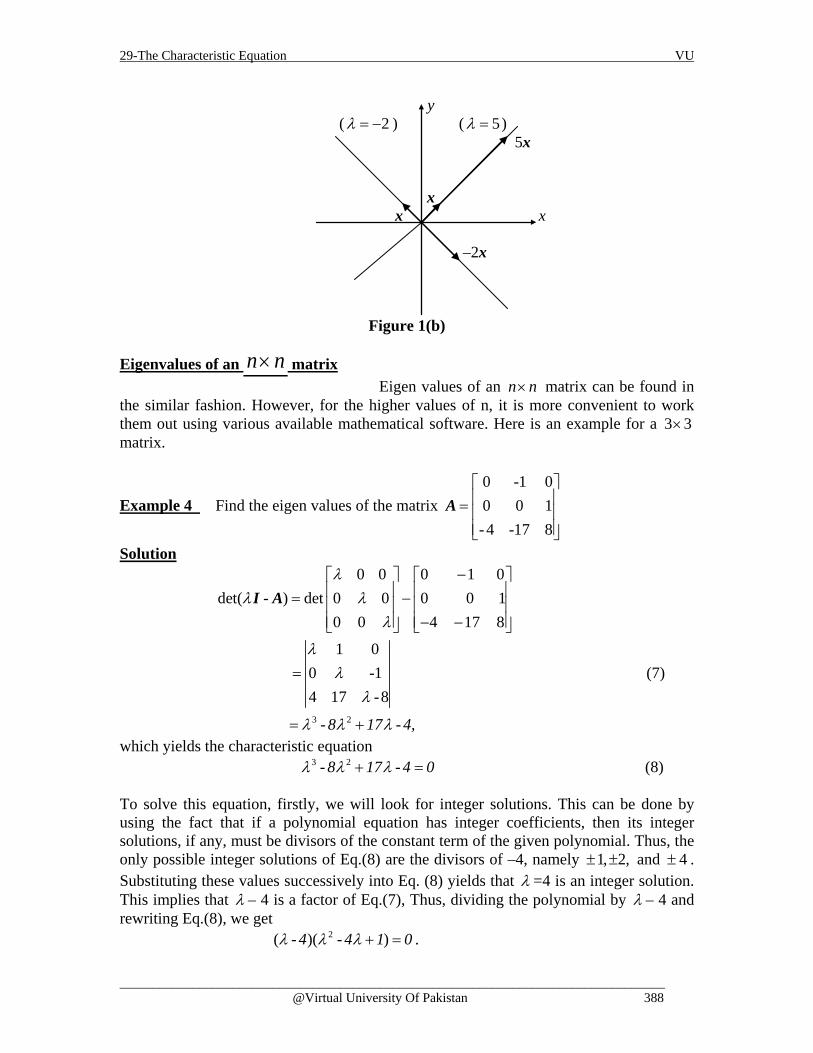
29-The Characteristic Equation VU
__________________________________________________________________________________ @Virtual University Of Pakistan 388
y ( 2λ = − ) ( 5λ = ) 5x
x x x
–2x
Figure 1(b)
Eigenvalues of an n n× matrix Eigen values of an n n× matrix can be found in the similar fashion. However, for the higher values of n, it is more convenient to work them out using various available mathematical software. Here is an example for a 3 3× matrix.
Example 4 Find the eigen values of the matrix 0 -1 00 0 1-4 -17 8
A =
Solution
3 2
0 0 0 1 0det( - ) det 0 0 0 0 1
0 0 4 17 8
1 00 -14 17 -8
- -8 17 4,
λλ λ
λ
λλ
λ
λ λ λ
− = − − −
=
= +
I A
(7)
which yields the characteristic equation 3 2- -+ =8 17 4 0λ λ λ (8)
To solve this equation, firstly, we will look for integer solutions. This can be done by using the fact that if a polynomial equation has integer coefficients, then its integer solutions, if any, must be divisors of the constant term of the given polynomial. Thus, the only possible integer solutions of Eq.(8) are the divisors of –4, namely 1, 2,± ± and 4± . Substituting these values successively into Eq. (8) yields that λ =4 is an integer solution. This implies that λ – 4 is a factor of Eq.(7), Thus, dividing the polynomial by λ – 4 and rewriting Eq.(8), we get 2( - )( - )+ =4 4 1 0λ λ λ .

29-The Characteristic Equation VU
__________________________________________________________________________________ @Virtual University Of Pakistan 389
Now, the remaining solutions of the characteristic equation satisfy the quadratic equation 2 - 4 1 0.λ λ + =
Solving the above equation by the quadratic formula, we get the eigenvalues of A as 4, 2 3, 2 3λ λ λ= = + = −
Example 5 Find the characteristic equation of
5 -2 6 -10 3 -8 00 0 5 40 0 0 1
=
A
Solution Clearly, the given matrix is an upper triangular matrix. Forming -A Iλ , we get
5 - -2 6 -10 3- -8 0
det( - ) det0 0 5 - 40 0 0 1-
A I
=
λλ
λλ
λ
Now using the fact that determinant of a triangular matrix is equal to product of its diagonal elements, the characteristic equation becomes 2(5 - ) (3- )(1- ) 0.λ λ λ = Expanding the product, we can also write it as 4 3 2-14 68 -130 75 0.λ λ λ λ+ + = Here, the eigenvalue 5 is said to have multiplicity 2 because (λ - 5) occurs two times as a factor of the characteristic polynomial. In general, the (algebraic) multiplicity of an eigenvalue λ is its multiplicity as a root of the characteristic equation. Note From the above mentioned examples, it can be easily observed that if A is an n n× matrix, then det (A – λ I) is a polynomial of degree n called the characteristic polynomial of A. Example 6 The characteristic polynomial of a 6 6× matrix is 6 5 4- 4 -12λ λ λ . Find the eigenvalues and their multiplicities. Solution In order to find the eigenvalues, we will factorize the polynomial as
6 5 4
4 2
4
- 4 -12( - 4 -12)( - 6)( 2)
λ λ λ
λ λ λ
λ λ λ
=
= +
The eigenvalues are 0 (multiplicity 4), 6 (multiplicity 1) and – 2 (multiplicity 1).We could also list the eigenvalues in Example 6 as 0, 0, 0, 0, 6 and –2, so that the eigenvalues are repeated according to their multiplicities

29-The Characteristic Equation VU
__________________________________________________________________________________ @Virtual University Of Pakistan 390
Activity Work out the eigenvalues and eigenvectors for the following square matrix.
5 8 164 1 8 .4 4 11
A = − − −
Similarity Let A and B be two n x n matrices, A is said to be similar to B if there exist an invertible matrix P such that P -1AP = B, or equivalently, A = PBP -1. Replacing Q by P -1, we have Q -1BQ = A. So B is also similar to A. Thus, we can say that A and B are similar. Similarity transformation The act of changing A into P -1AP is called a similarity transformation. The following theorem illustrates use of the characteristic polynomial and it provides the foundation for several iterative methods that approximate eigenvalues. Theorem 2 If n x n matrices A and B are similar, then they have the same characteristic polynomial and hence the same eigenvalues (with the same multiplicities). Proof If B = P -1AP, then
-1 -1 -1 -1 -1- - - ( - ) ( - )B I P AP I P AP P P P AP P P A I Pλ λ λ λ λ= = = = Using the multiplicative property (b) of Theorem 1, we compute
-1det( - ) det ( - )B I P A I Pλ λ =
-1det( ).det( - ).det( )P A I Pλ= (A) Since det (P -1). det(P) = det(P -1P) = det I = 1, Eq. (A) implies that det( - ) det( - ).B I A Iλ λ= Hence, both the matrices have the same characteristic polynomials and therefore, same eigenvalues. Note It must be clear that Similarity and row equivalence are two different concepts. ( If A is row equivalent to B, then B = EA for some invertible matrix E.) Row operations on a matrix usually change its eigenvalues.

29-The Characteristic Equation VU
__________________________________________________________________________________ @Virtual University Of Pakistan 391
Application to Dynamical Systems Dynamical system is the one which evolves with the passage of time. Eigenvalues and eigenvectors play a vital role in the evaluation of a dynamical system. Let’s consider an example of a dynamical system.
Example 7 Let .95 .03
..05 .97
A =
Analyze the long term behavior of the dynamical
system defined by xk+1 = Axk (k = 0, 1, 2, …), with 0.60.4
=
0x .
Solution The first step is to find the eigenvalues of A and a basis for each eigenspace. The characteristic equation for A is 0 det( )A Iλ= −
0.95 - 0.030 det (.95 - )(.97 - ) - (.03)(.05)
0.05 0.97 -λ
λ λλ
= =
2 -1.92 .92= +λ λ By the quadratic formula
21.92 (1.92) - 4(.92) 1.92 .00642 2
± ±= =λ 1.92 .08 1 or .92
2±
= =
Firstly, the eigenvectors will be found as given below. ,
( ) 0,( ) 0.
Ax xAx xA I x
λλλ
=− =− =
For 1λ =
1
2
1
2
0.95 0.03 1 00,
0.05 0.97 0 1
0.05 0.030,
0.05 0.03
xx
xx
− =
−
= −
which can be written as 1 2
1 2 1 2 1 2
0.05 0.03 00.03 30.05 0.03 0 .0.05 5
x x
x x x x or x x
− + =
− = ⇒ = =
In parametric form, it becomes
1 23 .5
x t and x t= =
For 0.92λ =

29-The Characteristic Equation VU
__________________________________________________________________________________ @Virtual University Of Pakistan 392
1
2
1
2
0.95 0.03 0.92 00,
0.05 0.97 0 0.92
0.03 0.030.
0.05 0.05
xx
xx
− =
=
It can be written as 1 2
1 2 1 2
0.03 0.03 00.05 0.05 0
x xx x x x+ =+ = ⇒ = −
In parametric form, it becomes 1 2x t and x t= = −
Thus, the eigenvectors corresponding to λ = 1 and λ = .92 are multiples of
3 1and
5 -1
= =
1 2v v respectively.
The next step is to write the given x0 in terms of v1 and v2. This can be done because {v1, v2} is obviously a basis for R2. So there exists weights c1 and c2 such that
11 2
2
[ ]0 1 2 1 2x v v v v
= + =
cc c
c (1)
In fact, 1
1 10
2
3 1 .60[ ]
5 -1 .401 2v v−
− = =
cx
c
Here, 13 1 3 1 1 11 1
3 15 1 5 1 5 385 1
Adj− − − = = − − − −
−
Therefore,
1
2
-1 -1 .60 .1251-5 3 .40 .225-8
cc
= =
(2)
Because v1 and v2 in Eq.(1) are eigenvectors of A, with Av1 = v1 and Av2 = (.92) v2, xk can be computed as
x1 = Ax0 = c1Av1 + c2Av2 (Using linearity of x Ax→ ) = c1v1 + c2 (.92)v2 (v1 and v2 are eigenvectors.) x2 = Ax1 = c1Av1 + c2 (.92)Av2 = c1v1 + c2 (.92)2 v2.
Continuing in the same way, we get the general equation as xk = c1v1 + c2(.92)kv2 (k = 0, 1, 2, …). Using c1 and c2 from Eq.(2),
3 1.125 .225(.92) ( 0,1,2,...)
5 -1kx = + =
k k (3)
This explicit formula for xk gives the solution of the difference equation xk+1 = Axk.

29-The Characteristic Equation VU
__________________________________________________________________________________ @Virtual University Of Pakistan 393
As k →∞ , (.92)k tends to zero and xk tends to .375
.125 ..625
=
1v
Example 8 Find the characteristic equation and eigenvalues of 1 -4
.4 2
A =
Solution The characteristic equation is 1- -4
0 det( - ) det4 2 -
A I = =
λλ
λ
2
(1- )(2 - ) - (-4)(4),-3 18,λ λ
λ λ
=
= +
which is a quadratic equation whose roots are given as
23 (-3) - 4(18)2
3 -632
λ±
=
±=
Thus, we see that the characteristic equation has no real roots, so A has no real eigenvalues. A is acting on the real vector space R2 and there is no non-zero vector v in R2 such that Av = λ v for some scalarλ .

29-The Characteristic Equation VU
__________________________________________________________________________________ @Virtual University Of Pakistan 394
Exercises Find the characteristic polynomial and the eigenvalues of matrices in exercises 1 to 12.
1. 3 21 1
− −
2. 5 34 3
− −
3. 2 11 4
−
4. 3 44 8
−
5. 5 34 4
−
6. 7 22 3
−
7. 1 0 12 3 10 6 0
− −
8. 0 3 13 0 21 2 0
9. 4 0 05 3 22 0 2
−
10. 1 0 13 4 1
0 0 2
− −
11. 6 2 02 9 0
5 8 3
− −
12. 5 2 30 1 06 7 2
− −
For the matrices in exercises 13 to 15, list the eigenvalues, repeated according to their multiplicities.
13.
4 7 0 20 3 4 60 0 3 80 0 0 1
− − −
14.
5 0 0 08 4 0 00 7 1 01 5 2 1
− −

29-The Characteristic Equation VU
__________________________________________________________________________________ @Virtual University Of Pakistan 395
15.
3 0 0 0 05 1 0 0 0
3 8 0 0 00 7 2 1 04 1 9 2 3
− − − −
16. It can be shown that the algebraic multiplicity of an eigenvalue λ is always greater than or equal to the dimension of the eigenspace corresponding to λ . Find h in the matrix A below such that the eigenspace for λ =5 is two-dimensional:
5 2 6 10 3 00 0 5 40 0 0 1
A
− − =
h

30-Diagonalization VU
__________________________________________________________________________________ @Virtual University Of Pakistan 396
Lecture 30
Diagonalization Diagonalization is a process of transforming a vector A to the form A = PDP-1 for some invertible matrix P and a diagonal matrix D. In this lecture, the factorization enables us to compute Ak quickly for large values of k which is a fundamental idea in several applications of linear algebra. Later, the factorization will be used to analyze (and decouple) dynamical systems. The “D” in the factorization stands for diagonal. Powers of such a D are trivial to compute.
Example 1 If 2
2
5 0 5 0 5 0 5 0, then
0 3 0 3 0 3 0 3
= = =
2D D and
2 3
2 3
5 0 5 0 5 00 3 0 3 0 3
= =
3D
In general, 5 0
for 10 3
k
k k
= ≥
kD
The next example shows that if A = PDP-1 for some invertible P and diagonal D, then it is quite easy to compute Ak.
Example 2 Let 7 2
.- 4 1
=
A Find a formula for Ak, given that A = PDP-1, where
1 1 5 0and
-1 -2 0 3
= =
P D
Solution The standard formula for the inverse of a 2 2× matrix yields 2 1-1 -1
=
-1P
By associative property of matrix multiplication, 1
1
( )( ) ( ) PDIDP−= = = =
2 -1 -1 -1 -1 -1A PDP PDP PD P P DP PDDP
where I is the identity matrix. 2
2
1 1 2 15 0-1 -2 -1 -10 3
= =
2 -1PD P
Again,
1
( ) ( )= = = =3 -1 2 -1 2 -1 2 -1 3 -1A PDP A PD P P D P PDD P PD P
Thus, in general, for 1,k ≥ 1 1 2 15 0
,-1 -2 -1 -10 3
k
k
= =
k k -1A PD P

30-Diagonalization VU
__________________________________________________________________________________ @Virtual University Of Pakistan 397
2 15 3
,-1 -15 2.3
k k
k k
= − −
2.5 -3 5 -3.
2.3 - 2.5 2.3 -5
k k k k
k k k k
=
Activity Work out 4C , given that 1C PDP−= where
1 0 2 0
,3 1 0 1
P D = =
Remarks A square matrix A is said to be diagonalizable if A is similar to a diagonal matrix, that is, if A = PDP-1 for some invertible matrix P and some diagonal matrix D. The next theorem gives a characterization of diagonalizable matrices and tells how to construct a suitable factorization. Theorem 1 The Diagonalization Theorem An n x n matrix A is diagonalizable if and only if A has n linearly independent eigenvectors. In fact, A = PDP-1, with D a diagonal matrix, if and only if the columns of P are n linearly independent eigenvectors of A. In this case, the diagonal entries of D are eigenvalues of A that correspond, respectively, to the eigenvectors in P. In other words, A is diagonalizable if and only if there are enough eigenvectors to form a basis of Rn. We call such a basis an eigenvector basis. Proof First, observe that if P is any n n× matrix with columns v1, … , vn and if D is any diagonal matrix with diagonal entries 1,...., nλ λ then
[ ] [ ]... ... ,= =1 2 n 1 2 nAP A v v v Av Av Av (1)
while [ ]1
21 2
0 00 0
0 0
n
n
λλ
λ λ λ
λ
= =
1 2 nPD P v v v
(2)
Suppose now that A is diagonalizable and A = PDP-1. Then right-multiplying this relation by P, we have AP = PD. In this case, (1) and (2) imply that
[ ] [ ]1 2 nλ λ λ=1 2 n 1 2 nAv Av Av v v v (3) Equating columns, we find that
1 2, , , nλ λ λ= = =1 1 2 2 n nAv v Av v Av v (4) Since P is invertible, its columns v1,…, vn must be linearly independent. Also, since these columns are nonzero, Eq.(4) shows that 1,....., nλ λ are eigenvalues and v1, …, vn are

30-Diagonalization VU
__________________________________________________________________________________ @Virtual University Of Pakistan 398
corresponding eigenvectors. This argument proves the “only if” parts of the first and second statements along with the third statement, of the theorem. Finally, given any n eigenvectors v1, …, vn use them to construct the columns of P and use corresponding eigenvalues 1,....., nλ λ to construct D. By Eqs. (1) – (3). AP =PD. This is true without any condition on the eigenvectors. If, in fact, the eigenvectors are linearly independent, then P is invertible (by the Invertible Matrix Theorem), and AP = PD implies that A = PDP-1. Diagonalizing Matrices
Example 3 Diagonalize the following matrix, if possible 1 3 3-3 -5 -33 3 1
=
A
Solution To diagonalize the given matrix, we need to find an invertible matrix P and a diagonal matrix D such that A = PDP-1 which can be done in following four steps. Step 1 Find the eigenvalues of A. The characteristic equation becomes
3 20 det( ) 3 4A Iλ λ λ= − = − − + 2( 1)( 2)λ λ= − − + The eigenvalues are λ = 1 and λ = -2 (multiplicity 2) Step 2 Find three linearly independent eigenvectors of A. Since A is a 3 3× matrix and we have obtained three eigen values, we need three eigen vectors. This is the critical step. If it fails, then above Theorem says that A cannot be diagonalized. Now we will produce basis for these eigen values. Basis vector for 1:λ =
1
2
3
( ) 00 3 3 03 6 3 0 .
3 3 0 0
A I xxxx
λ− =
− − − =
After applying few row operations on the matrix ( )A Iλ− , we get
1
2
3
0 1 1 03 3 0 0 ,0 0 0 0
xxx
=
which can be written as 2 3
1 2
03 3 0x xx x+ =+ =
In parametric form, it becomes 1 2 3, ,x t x t x t= = − =

30-Diagonalization VU
__________________________________________________________________________________ @Virtual University Of Pakistan 399
Thus, the basis vector for 1λ = is 1
11
1v
= −
Basis vector for -2λ =
1
2
3
( ) 03 3 3 03 3 3 0 ,
3 3 3 0
A I xxxx
λ− =
− − − =
which can be written as
1 2 3
1 2 3
1 2 3
3 3 3 03 3 3 0
3 3 3 0
x x xx x x
x x x
+ + =
− − − =+ + =
In parametric form, it becomes 1 2 3, ,x s t x s x t= − − = =
Now, 1
2
3
2 3
0 ,0
1 11 0 ,0 1
1 11 0 .0 1
x s t s tx s sx t t
s t
x x
− − − − = = +
− − = + − − = +
Thus, the basis for 2λ = − is 2
110
v− =
and 3
101
v− =
We can check that {v1, v2, v3} is a linearly independent set. Step 3 Check that {v1, v2, v3} is a linearly independent set. Construct P from the vectors in step 2. The order of the vectors is not important. Using
the order chosen in step 2, form 1 -1 -1
[ ] -1 1 01 0 1
1 2 3P v v v = =

30-Diagonalization VU
__________________________________________________________________________________ @Virtual University Of Pakistan 400
Step 4 Form D from the corresponding eigen values. For this purpose, the order of the eigen values must match the order chosen for the columns of P. Use the eigen value λ = -2 twice, once for each of the eigenvectors corresponding to λ = -2:
1 0 00 -2 00 0 -2
D =
Now, we need to check do P and D really work. To avoid computing P -1, simply verify that AP = PD. This is equivalent to A = PDP -1 when P is invertible.We compute
1 3 3 1 -1 -1 1 2 2-3 -5 -3 -1 1 0 -1 -2 03 3 1 1 0 1 1 0 -2
1 -1 -1 1 0 0 1 2 2-1 1 0 0 -2 0 -1 -2 01 0 1 0 0 -2 1 0 -2
AP
PD
= = = =
Example 4 Diagonalize the following matrix, if possible.
2 4 3-4 -6 -33 3 1
=
A
Solution The characteristic equation of A turns out to be exactly the same as that in example 3 i.e.,
3 2
2
0 det( - )2 4 3
4 6 33 3 1
- -3 4-( -1)( 2)
λλ
λλ
λ λ
λ λ
=
−= − − − −
−
= +
= +
A I
The eigen values are λ = 1 and λ = -2 (multiplicity 2). However, when we look for eigen vectors, we find that each eigen space is only one – dimensional.
Basis for 1
1: -11
1v = =
λ
Basis for -1
-2 : 10
2v = =
λ

30-Diagonalization VU
__________________________________________________________________________________ @Virtual University Of Pakistan 401
There are no other eigen values and every eigen vector of A is a multiple of either v1 or v2. Hence it is impossible to form a basis of R3 using eigenvectors of A. By above Theorem, A is not diagonalizable. Theorem 2 An n x n matrix with n distinct eigenvalues is diagonalizable. The condition in Theorem 2 is sufficient but not necessary i.e., it is not necessary for an n x n matrix to have n distinct eigen values in order to be diagonalizable. Example 3 serves as a counter example of this case where the 3 x 3 matrix is diagonalizable even though it has only two distinct eigen values. Example 5 Determine if the following matrix is diagonalizable.
5 -8 10 0 70 0 -2
A =
Solution In the light of Theorem 2, the answer is quite obvious. Since the matrix is triangular, its eigen values are obviously 5, 0, and –2.Since A is a 3 x 3 matrix with three distinct eigen values, A is diagonalizable. Matrices Whose Eigenvalues Are Not Distinct If an n x n matrix A has n distinct eigen values, with corresponding eigen vectors v1 ,..., v n and if P = [v1 … vn] , then P is automatically invertible because its columns are linearly independent , by Theorem 2 of lecture 28. When A is diagonalizable but has fewer than n distinct eigen values, it is still possible to build P in a way that makes P automatically invertible, as shown in the next theorem. Theorem 3 Let A be an n x n matrix whose distinct eigen values are 1λ λ p, ..., .
a. For 1≤ k≤ p, the dimension of the eigen space for λk is less than or equal to the multiplicity of the eigen value λk
b. The matrix A is diagonalizable if and only if the sum of the dimensions of the distinct eigen spaces is equal to n, and this happens if and only if the dimension of the eigen space for each of λk equals the multiplicity of λk .
c. If A is diagonalizable and Bk is basis for the eigen space corresponding to λk for each k, then the total collection of vectors in the sets B1, ..., Bp form an eigenvector basis for Rn .
Example 6 Diagonalize the following matrix, if possible.

30-Diagonalization VU
__________________________________________________________________________________ @Virtual University Of Pakistan 402
5 0 0 00 5 0 01 4 -3 0-1 -2 0 -3
A
=
Solution Since A is triangular matrix, the eigenvalues are 5 and –3, each with multiplicity 2. Using the method of lecture 28, we find a basis for each eigen space.
Basis for 1 2
-8 -164 4
λ 5 : and1 00 1
v v
= = =
Basis for 3 4
0 00 0
λ -3 : and1 00 1
v v
= = =
The set {v1,…,v4}is linearly independent, by Theorem 3. So the matrix P =[v1…v4] is invertible, and A=PDP -1 , where
-8 -16 0 0 5 0 0 04 4 0 0 0 5 0 0
and1 0 1 0 0 0 -3 00 1 0 1 0 0 0 -3
P D
= =
Example 7
(1) Compute A8 where 4 -32 -1
A =
(2) Let 1 2
-3 12 3 2, and
-2 7 1 1A v , v = = =
. Suppose you are told that v1 and
v2 are eigenvectors of A. Use this information to diagonalize A. (3) Let A be a 4 x 4 matrix with eigenvalues 5, 3, and -2, and suppose that you
know the eigenspace for λ=3 is two-dimensional. Do you have enough information to determine if A is diagonalizable?
Solution Here, det (A-λ I)=λ 2 -3λ+2=(λ -2)(λ -1).

30-Diagonalization VU
__________________________________________________________________________________ @Virtual University Of Pakistan 403
The eigen values are 2 and 1, and corresponding eigenvectors are
1 2
3 1, and
2 1v v = =
. Next, form
13 1 2 0 1 -1, and
2 1 0 1 -2 3−
= = =
P ,D P
Since A = PDP –1, A8 = PD8P8
8
3 1 1 -12 02 1 -2 30 1
=
3 1 256 0 1 -12 1 0 1 -2 3
=
766 -765510 -509
=
(2)Here, 1 1
-3 12 3 31 ,
-2 7 1 1Av .v
= = =
and
2 2
-3 12 2 63
-2 7 1 3Av .v
= = =
Clearly, v1 and v2 are eigenvectors for the eigenvalues 1 and 3 , respectively. Thus
A = PDP -1, where 3 2 1 0
and1 1 0 3
P D = =
(3) Yes A is diagonalizable. There is a basis {v1, v2 } for the eigen space corresponding to λ=3. Moreover, there will be at least one eigenvector for λ=5 and one for λ=-2 say v3 and v4. Then {v1, …., v4 } is linearly independent and A is diagonalizable , by Theorem 3. There can be no additional eigen vectors that are linearly independent from v1 to v4 because the vectors are all in R4 .Hence the eigenspaces for λ=5 and λ=-2 are both one–dimensional.

30-Diagonalization VU
__________________________________________________________________________________ @Virtual University Of Pakistan 404
Exercise In exercises 1 and 2, let A = PDP-1 and compute A4.
1. 5 7 2 0
,2 3 0 1
P D = =
2. 2 3 1 0
,3 5 0 1/2
P D =−
= −
In exercises 3 and 4, use the factorization A = PDP-1 to compute Ak, where k represents an arbitrary positive integer.
3. 0 1 0 0 1 0
3( ) 3 1 0 3 1
= − −
a aa b b b
4. 2 12 3 4 2 0 1 41 5 1 1 0 1 1 3
− − = − −
In exercises 5 and 6, the matrix A is factored in the form PDP-1. Use the Diagonalization Theorem to find the eigenvalues of A and a basis for each eigenspace.
5. 2 2 1 1 1 2 5 0 0 1 4 1 2 1 41 3 1 1 0 1 0 1 0 1 4 1 2 3 41 2 2 1 1 0 0 0 1 1 4 1 2 1 4
/ / // / // / /
= − − − −
6. 4 0 2 2 0 1 5 0 0 0 0 12 5 4 0 1 2 0 5 0 2 1 40 0 5 1 0 0 0 0 4 1 0 2
− − − = − −
Diagonalize the matrices in exercises 7 to 18, if possible.
7. 3 11 5
−
8. 2 34 1
9. 1 4 23 4 03 1 3
− − − −
10. 4 2 22 4 22 2 4

30-Diagonalization VU
__________________________________________________________________________________ @Virtual University Of Pakistan 405
11. 2 2 11 3 11 2 2
− − − −
12. 4 0 22 5 40 0 5
−
13. 7 4 162 5 82 2 5
− − −
14. 0 4 61 0 3
1 2 5
− − − −
15. 4 0 01 4 00 0 5
16. 7 16 4
6 13 212 16 1
− − −
17.
5 3 0 90 3 1 20 0 2 00 0 0 2
− −
18.
4 0 0 00 4 0 00 0 2 01 0 0 2

31-Eigenvectors and Linear Transformations VU
©Virtual University Of Pakistan 406
Lecture 31
Eigenvectors and Linear Transformations The goal of this lecture is to investigate the relationship between eigenvectors and linear transformations. Previously, we have learned how to find the eigenvalues and eigenvectors. We shall see that the matrix factorization A = PDP - 1 is also a type of linear transformations for some invertible matrix P and some diagonal matrix D. The Matrix of a Linear Transformation Let V be an n-dimensional vector space, W an m-dimensional vector space, and T any linear transformation from V to W. To associate a matrix with T, we choose (ordered) bases B and C for V and W, respectively. Given any x in V, the coordinate vector [x]B is in Rn and the coordinate vector of its image, [T(x)]C, is in Rm, as shown in Fig. 1.
Figure 1 A linear transformation from V to W
Let B={b1, …, bn} be the basis for V. If x = r1b1 ++ rnbn,
then 1
[ ]Bx =
n
r
r
and T is a linear transformation 1 1( ) ( ) ( ) ( )1 n 1 nT x T b b T b T b= + + = + + n nr r r r (1)

31-Eigenvectors and Linear Transformations VU
©Virtual University Of Pakistan 407
Using the basis C in W, we can rewrite (1) in terms of C-coordinate vectors: 1[ ( )] [ ( )] [ ( )]C 1 C n CT x T b T b= + + nr r (2)
Since C-coordinate vectors are in Rm, the vector equation (2) can be written as a matrix equation, namely
[ ( )] [ ]C BT x M x= (3) where [ ][ ( )] [ ( )] [ ( )]1 C 2 C n CM T b T b T b= (4) The matrix M is a matrix representation of T, called the matrix for T relative to the bases B and C.
Figure 2 Example 1 Suppose that B = {b1, b2} is a basis for V and C = {c1, c2, c3} is a basis for W. Let
:T V W→ be a linear transformation with the property that ( ) 3 - 2 5 and ( ) 4 7 -1 1 2 3 2 1 2 3T b c c c T b c c c= + = +
Find the matrix M for T relative to B and C. Solution Since [ ][ ( )] [ ( )] [ ( )]= 1 C 2 C n CM T b T b T b and here
3 4[ ( )] -2 and [ ( )] 7
5 -11 C 2 CT b T b
= =
Hence, 3 4-2 75 -1
M =

31-Eigenvectors and Linear Transformations VU
©Virtual University Of Pakistan 408
Linear Transformations from V into V In general when W is the same as V and the basis C is the same as B, the matrix M in (4) is called the matrix for T relative to B, or simply the B-matrix for T, is denoted by [T]B. See Fig. 3.
Figure 3
The B-matrix of :T V V→ satisfies
[ ( )] [ ] [ ] ,B B BT x T x= for all x in V (5) Example 2 The mapping : 2 2T P P→ defined by 1 2 2( ) 22
0 1T a t t a t+ + = +a a a is a linear transformation. (a) Find the B-matrix for T, when B is the basis {1, t, t2}. (b) Verify that [T(p)]B = [T]B[p]B for each p in P2. Solution (a) We have to find the B-matrix of :T V V→ satisfies [ ( )] [ ] [ ] ,B B BT x T x= for all x in V Since 1 2 2( ) 2a a a+ + = +2
0 1T a t t a t therefore
T (1) = 0 , T (t) = 1, T (t2) = 2t

31-Eigenvectors and Linear Transformations VU
©Virtual University Of Pakistan 409
2
0 1 0[ ( )] 0 , [ ( )] 0 , [ ( )] 2
0 0 0B B BT 1 T t T t
= = =
0 1 0[ ] 0 0 2
0 0 0BT
=
(b) For a general p (t) = a0 +a1t +a2t2, we have
1
2 2[ ( )] [ 2 ] 20
B 1 BT p a t = + =
aa a
0
1
2
0 1 00 0 2 [ ] [ ]0 0 0
B BT p = =
aaa
See figure 4.
Figure 4 Matrix representation of a linear transformation Linear Transformations on Rn In an applied problem involving Rn, a linear transformation T usually appears first as a matrix transformation, x Ax→ . If A is diagonalizable then there is a basis B for Rn consisting of eigenvectors of A. Theorem below shows that in this case, the B-matrix of T is diagonal. Diagonalizing A amounts to finding a diagonal matrix representation of x Ax→ .

31-Eigenvectors and Linear Transformations VU
©Virtual University Of Pakistan 410
Theorem: Diagonal Matrix Representation Suppose A = PDP -1, where D is diagonal n x n matrix. If B is the basis for Rn formed from the columns of P, then D is the B-matrix of the transformation x Ax→ . Proof Denote the columns of P by b1, …, bn, so that B = {b1, …, bn} and P = [b1 … bn]. In this case, P is the change-of-coordinates matrix PB discussed in lecture 23, where [ ] and [ ] -1
B BP x x x P x= = If T (x) = Ax for x in Rn, then
[ ][ ] [ ( )] [ ( )]B 1 B n BT T b T b= Definition of [T]B
[ ][ ] [ ]1 B n BAb Ab= Since T (x) = Ax -1 -1
1 nP Ab P Ab = Change of Coordinates
[ ]-11 nP A b b= Matrix multiplication
-1P AP= (6) Since A = PDP-1, we have [T]B = P -1AP = D. Example 3
Define : 2 2T R R→ by T (x) = Ax, where 7 2
.- 4 1
A =
Find a basis B for R2 with the
property that the B-matrix of T is a diagonal matrix. Solution Since the eigenvalues of matrix A are 5 and 3 and the eigenvectors corresponding to
eigenvalue 5 is 11
−
and the eigenvectors corresponding to eigenvalue 3 is 12
−
Therefore A = PDP -1, where 1 1 5 0
and-1 -2 0 3
= =
P D
By the above theorem D matrix is the B matrix of T when B= 1 1
,1 2
− −
.
Similarity of Matrix Representations We know that A is similar to C if there is an invertible matrix P such that A = PCP -1, therefore if A is similar to C , then C is the B-matrix of the transformation
→x Ax when the basis B is formed from the columns of P by the theorem above.(Since in the proof , the information that D is a diagonal matrix was not used). The factorization A = PCP -1 is shown in Fig. 5.

31-Eigenvectors and Linear Transformations VU
©Virtual University Of Pakistan 411
Figure 5 Similarity of two matrix representations: A = PCP -1
Conversely, if : n nT R R→ is defined by T (x) = Ax, and if B is any basis for Rn, then the B-matrix of T is similar to A. In fact, the calculations in (6) show that if P is the matrix whose columns come from the vectors in B, then [T]B = P -1AP. Thus, the set of all matrices similar to a matrix A coincides with the set of all matrix representations of the transformation .x Ax→
An efficient way to compute a B-matrix P -1AP is to compute AP and then to row reduce the augmented matrix [P AP] to [I P -1AP]. A separate computation of P -1 is unnecessary. Example 4 Find T ( a0 + a1t + a2 t2 ), if T is the linear transformation from P2 to P2 whose matrix
relative to B ={1, t, t2} is 3 4 0
[ ] 0 5 11 2 7
BT = − −
Solution Let p(t) = a0 + a1t + a2 t2 and compute
0 0 1
1 1 2
2 0 1 2
3 4 0 3 4[ ( )] [ ] [ ] 0 5 1 5
1 2 7 2 7B B B
a a aT p T p a a a
a a a a
+ = = − = − − − +
So T (p) = (3a0+4a1)1 + (5a1-a2)t + (a0-2a1+7a2)t2 .

31-Eigenvectors and Linear Transformations VU
©Virtual University Of Pakistan 412
Example 5 Let A, B, C be n x n matrices. Verify that (a) A is similar to A. (b) If A is similar to B and B is similar to C, then A is similar to C. Solution (a) A =(I)-1AI, so A is similar to A. (b) By hypothesis, there exist invertible matrices P and Q with the property that B = P -1 AP and C = Q -1BQ. Substituting, and using facts about the inverse of a product we have
1 1 1 1( ) ( ) ( )C Q BQ Q P AP Q PQ A PQ− − − −= = = This equation has the proper form to show that A is similar to C.

32-Complex Eigenvalues VU
©Virtual University Of Pakistan 413
Lecture 32
Eigenvalues and Eigenvectors
Definition A complex scalar λ satisfies det(A- λI ) = 0 if and only if there is a nonzero vector x in Cn such that Ax= λx. We call λ a (complex) eigenvalue and x a (complex) eigenvector corresponding to λ. Example 1
If 0 -1
,1 0
A =
then the linear transformation x Ax→ on R2 rotates the plane
counterclockwise through a quarter-turn. Solution The action of A is periodic since after four quarter-turns, a vector is back where it started. Obviously, no nonzero vector is mapped into a multiple of itself, so A has no eigenvectors in R2 and hence no real eigenvalues. In fact, the characteristic equation of A is 2 21 0 1 iλ λ λ+ = ⇒ = − ⇒ = ± The only roots are complex: iλ = and .iλ = − However, if we permit A to act on C2 then
0 -1 1 11 0 - 1 -
= =
ii
i i
0 -1 1 - 1-
1 0 1
= =
ii
i i
Thus i and –i are the eigenvalues, with 1-
i
and1i
as corresponding eigenvectors.
Example 2
Let 0.5 -0.60.75 1.1
=
A .Find the eigenvalues of A, and find a basis for each eigen-space.
Solution The characteristic equation of A is
0.5 0.60 det (0.5 )(1.1 ) ( 0.6)(0.75)
0.75 1.1λ
λ λλ
− − = = − − − − −
2 1.6 1λ λ= − +

32-Complex Eigenvalues VU
©Virtual University Of Pakistan 414
From the quadratic formula, 212 [1.6 ( 1.6) 4] 0.8 0.6 .iλ = ± − − = ± For the eigenvalue
0.8 0.6 ,iλ = − we study 0.5 0.6 0.8 0.6 0
(0.8 0.6 )0.75 1.1 0 0.8 0.6
ii
i− −
− − = − − A
0.3 0.6 0.60.75 0.3 0.6
ii
− + − = +
(1)
Since 0.8 – 0.6i is an eigenvalue, we know that the system 1 2( 0.3 0.6 ) 0.6 0i x x− + − =
1 20.75 (0.3 0.6 ) 0x i x+ + = (2) has a nontrivial solution (with x1 and x2 possibly complex numbers). 1 20.75 ( 0.3 0.6 )x i x= − − ⇒ 1 2( 0.4 0.8 )x i x= − − Taking x2 = 5 to eliminate the decimals, we have x1 = –2 – 4i. A basis for the eigenspace
corresponding to λ = 0.8 – 0.6i is 2 4
51v− −
=
i
Analogous calculations for λ =0 .8 + 0.6i produce the eigenvector 2 4
52v− +
=
i
Check Compute
0.5 0.6 2 4 4 2(0.8 0.6 )
0.75 1.1 5 4 3i i
ii
− − + − + = = = + +
2 2Av v
Example 3 One way to see how multiplication by the A in Example 2 affects points is to plot an arbitrary initial point-say, x0 = (2, 0) and then to plot successive images of this point under repeated multiplications by A. That is, plot
0.5 0.6 2 1.0.75 1.1 0 1.5
− = = =
1 0x Ax
0.5 0.6 1.0 0.4
=0.75 1.1 1.5 2.4
− − = =
2 1x Ax
,3 2x Ax= Figure 1 shows x0, …, x8 as heavy dots. The smaller dots are the locations of x9, …, x100. The sequence lies along an elliptical orbit.
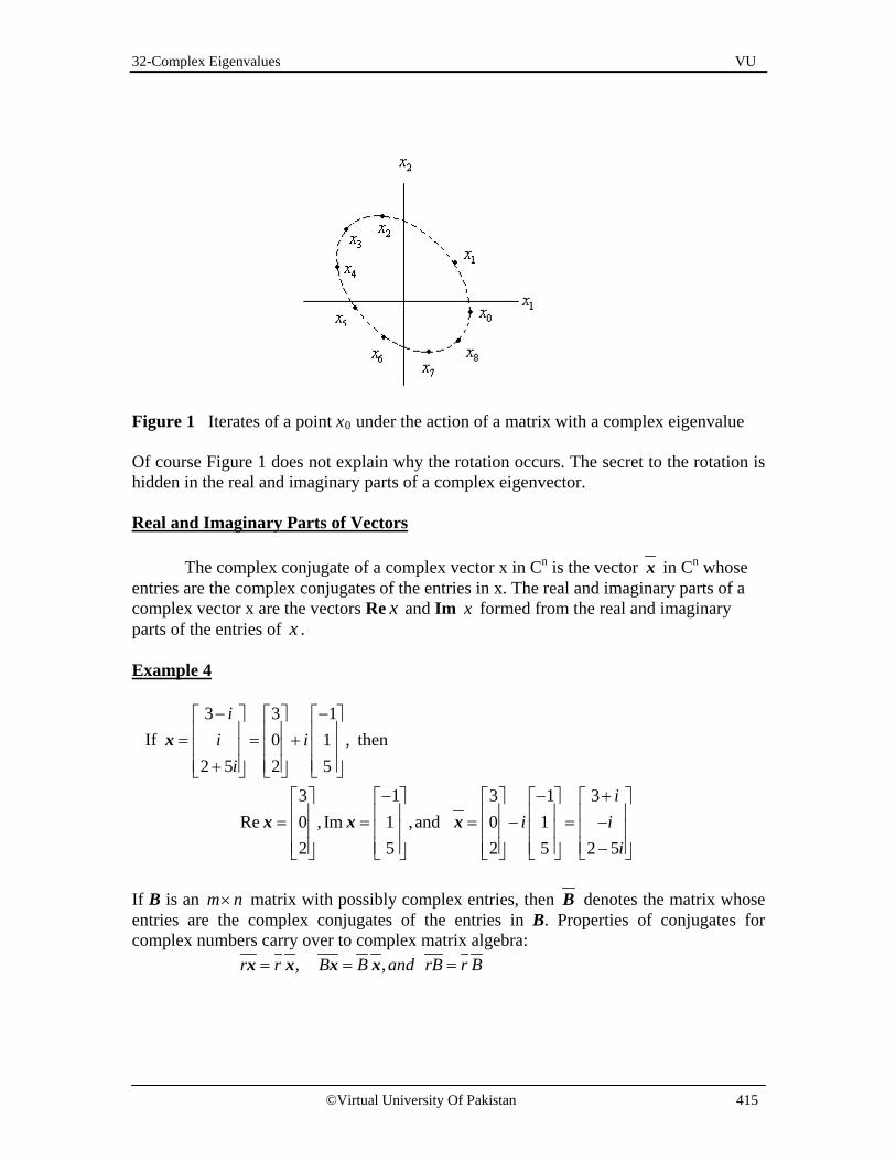
32-Complex Eigenvalues VU
©Virtual University Of Pakistan 415
Figure 1 Iterates of a point x0 under the action of a matrix with a complex eigenvalue Of course Figure 1 does not explain why the rotation occurs. The secret to the rotation is hidden in the real and imaginary parts of a complex eigenvector. Real and Imaginary Parts of Vectors
The complex conjugate of a complex vector x in Cn is the vector x in Cn whose
entries are the complex conjugates of the entries in x. The real and imaginary parts of a complex vector x are the vectors Re x and Im x formed from the real and imaginary parts of the entries of x . Example 4
If 3 3 1
0 1 ,2 5 2 5
x− −
= = + +
ii i
i then
3 1 3 1 3Re 0 , Im 1 ,and 0 1
2 5 2 5 2 5x x x
− − + = = = − = − −
ii i
i
If B is an m n× matrix with possibly complex entries, then B denotes the matrix whose entries are the complex conjugates of the entries in B. Properties of conjugates for complex numbers carry over to complex matrix algebra:
, ,r r B B and rB r B= = =x x x x

32-Complex Eigenvalues VU
©Virtual University Of Pakistan 416
Eigenvalues and Eigenvectors of a Real Matrix that Acts on Cn
Let A be n n× matrix whose entries are real. Then .A A A= =x x x If λ is an eigenvalue of A with x a corresponding eigenvector in Cn, then A A λ λ= = =x x x x Hence λ is also an eigenvalue of A, with x a corresponding eigenvector. This shows that when A is real, its complex eigenvalues occur in conjugate pairs. (Here and elsewhere, we use the term complex eigenvalue to refer to an eigenvalue a biλ = + with 0b ≠ .) Example 5 The eigenvalues of the real matrix in example 2 are complex conjugates namely, 0.8 – 0.6i and 0.8 + 0.6i. The corresponding eigenvectors found in example 2 are also
conjugates: 2 4 2 4
and5 5
11 2v v v− − − +
= = =
i i
Example 6
If C−
=
a bb a
, where a and b are real and not both zero, then the eigenvalues of C are
.a biλ = ± Also, if 2 2r a bλ= = + , then
Figure 2
/ / 0 cos sin/ / 0 sin cos
C− −
= =
a r b r rr
b r a r rϕ ϕϕ ϕ
where ϕ is the angle between the positive x-axis and the ray from (0, 0) through (a, b). See Fig. 2. The angle ϕ is called the argument of .= +a biλ

32-Complex Eigenvalues VU
©Virtual University Of Pakistan 417
Thus, the transformation x Cx→ may be viewed as the composition of a rotation through the angle ϕ and a scaling by λ .
Figure 3 A rotation followed by a scaling
Finally, we are ready to uncover the rotation that is hidden within a real matrix having a complex eigenvalue. Example 7
Let 0.5 0.6
, 0.8 0.6 ,0.75 1.1
iλ−
= = −
A and 2 4
,51v
− − =
i as in example 2. Also, let P
be the 2 2× real matrix [ ] 2 4Re Im
5 01 1P v v− −
= =
and let 0 4 0.5 0.6 2 4 0.8 0.615 2 0.75 1.1 5 0 0.6 0.820
− − − − = = = − −
-1C P AP
By Example 6, C is a pure rotation because 2 2 2(.8) (.6) 1.λ = + = From C = P -1AP, we obtain
0.8 0.60.6 0.8
− = =
-1 -1A PCP P P
Here is the rotation “inside” A! The matrix P provides a change of variable, say, x = Pu. The action of A amounts to a change of variable from x to u, followed by a rotation, and then return to the original variable. See Figure 4.

32-Complex Eigenvalues VU
©Virtual University Of Pakistan 418
Figure 4 Rotation due to a complex eigenvalue Theorem Let A be a real 2 x 2 matrix with complex Eigen values ( 0)ia b bλ = − ≠ and associated eigenvectors v in 2
, then
[ ]
1, ,
Re Im
a bA PCP C
b a
P v v
− − = =
=

33-Discrete Dynamical Systems VU
©Virtual University Of Pakistan 419
Lecture 33
Discrete Dynamical Systems For a dynamical system described by the difference equation
1x Axk k=+ ,eigenvalues and eigenvectors provide the key to understand the long term
behavior and evolution of the system. Here the vector xk gives information about the system as time (which is denoted by k) passes. Discrete dynamical system has a great application in many scientific fields. For example, modern state space design method of standard undergraduate courses in control system and steady state response of a control system relies heavily on dynamical system. In this section, we will suppose that a matrix A is diagonalizable, with n linearly independent eigenvectors, 1v , …, vn, and corresponding eigenvalues
1 2, ,... nλ λ λ . For convenience, assume that the eigenvectors are arranged so that 1 2 ... nλ λ λ≥ ≥ ≥
Since { 1v , …, vn } is a basis for nR , any initial vector 0x can be written uniquely as 0 1 1 2 2 ... n nx c v c v c v= + + + Since the vi are eigenvectors,
1 0
1 1 2 2
1 1 1 2 2 2
......
n n
n n n
x Axc Av c Av c Avc v c v c vλ λ λ
== + + += + + +
In general, 1 1 1( ) ... ( ) ( 0,1, 2...)k k
k n n nx c v c v kλ λ= + + = We will discuss in the following examples what can happen to kx if k→ ∞ . Example 1
Denote the owl and wood rat populations at time k by ,kx
=
k
k
OR
where k is the time in
months, Ok is the number of owls in the region studied, and Rk is the number of rats (measured in thousands). Suppose that
1
1
(.5) (.4)(1.1)
k k k
k k k
O O RR p O R
+
+
= += − ⋅ +
where p is a positive parameter to be specified. The (.5)Ok in the first equation says that with no wood rats for food only half of the owls will survive each month, while the (1.1)Rk in the second equation says that with no owls as predators, the rat population will grow by 10% per month. If rats are plentiful, then (.4)Rk will tend to make the owl population rise, while the negative term –p.Ok measures the deaths of rats due to

33-Discrete Dynamical Systems VU
©Virtual University Of Pakistan 420
predation by owls. (In fact, 1000p is the average number of rats eaten by one owl in one month.) Determine the evolution of this system when the predation parameter p is 0.104. Solution The coefficient matrix A for the given equations is
0.5 0.41.1
Ap
= −
When p = .104, The matrix becomes
0.5 0.40.104 1.1
A = −
For eigenvalues of the coefficient matrix put det ( )A Iλ− =0 The eigenvectors corresponding to the eigenvalues 1 1.02λ = and 2 .58λ = are
10 5,
13 11 2v v = =
.
An initial x0 can be written as x0 = c1v1 + c2v2 then, for 0k ≥ ,
1 2(1.02) (.58)k 1 2x v v= +k kc c 1 2
10 5(1.02) (.58)
13 1k kc c
= +
As , (.58)kk → ∞ rapidly approaches zero. Assume 1 0.c ≠ Then, for all sufficiently large k, xk is approximately the same as c1(1.02)kv1, and we write
1
10(1.02)
13kx ≈
kc ……………….(1)
The approximation in (1) improves as k increases, and so for large k,
11 1
10 10(1.02) (1.02) (1.02) 1.02
13 13k kc c+
≈ = ≈
k+1 kx x
This approximation says that eventually both xk entries i.e owls and rats grow by a factor of almost 1.02 each month. Also equation (1) shows that xk is approximately a multiple of (10,13).So we can say that the entries in xk are almost in the same ratio as 10 to 13.It means that for every 10 owls there are about 13 thousand rats. Trajectory of a dynamical system In a 2×2 matrix, geometric description of a system’s evolution can enhance the algebraic calculations. We can view that what happens to an initial point x0 in 2R , when it is transformed repeatedly by the mapping x→Ax. The graph of x0, x1…is called a trajectory of the dynamical system.

33-Discrete Dynamical Systems VU
©Virtual University Of Pakistan 421
Example 2 Plot several trajectories of the dynamical system xk+1 = Axk, when
.80 00 .64
A =
Solution In a diagonal matrix the eigen values are the diagonal entries and as A is a diagonal matrix with diagonal enteries 0.8 and 0.64,Therefore the eigenvalues of A are .8 and .64,
with eigenvectors 101v
=
and 0
.12v
=
If x0 = c1v1 + c2v2, then 1 2
1 0(.8) (.64)
0 1kx = +
k kc c
Of course, xk tends to 0 because (.8)k and (.64)k both approach to 0 as .k → ∞ But the way xk goes towards 0 is interesting. Figure 1 shows the first few terms of several trajectories that begin at points on the boundary of the box with corners at ( 3, 3).± ± The points on a trajectory are connected by a thin curve, to make the trajectory easier to see.
Figure 1 The origin as an attractor In this example, the origin is called an attractor of the dynamical system because all trajectories tend towards O. This occurs whenever both eigenvalues are less than 1 in magnitude. The direction of greatest attraction is along the line through O and the eigenvector v2 as it has smaller eigenvalue.

33-Discrete Dynamical Systems VU
©Virtual University Of Pakistan 422
Example 3 Plot several typical solution of the equation 1k kx Ax+ = , when
1.44 00 1.2
A =
Solution In a diagonal matrix the eigen values are the diagonal entries and as A is a diagonal matrix with diagonal entries 1.44 and 1.2,Therefore the eigenvalues of A are 1.44 and
1.2, with eigenvectors 101v
=
and 0
.12v
=
As
0 1 1 2 2
1 2
1
2
1
2
1 00 1
00
,
x c v c v
c c
cc
cthen
c
= +
= +
= +
=
1 2
1 0(1.44) (1.2)
0 1k k
kx c c = +
Both terms grow in size as k→ ∞ ,but the first term grows faster because it has larger eigenvalue. Figure 2 shows several trajectories that begin at points quite close to 0.
Figure 2 The origin as a repellor In this example, the origin is called a repellor of the dynamical system because all trajectories tend away from O. This occurs whenever both eigenvalues are greater than 1

33-Discrete Dynamical Systems VU
©Virtual University Of Pakistan 423
in magnitude. The direction of the greatest repulsion is the line through 0 and that eigen vector which has a larger eigenvalue. Remark From the above two examples it may be noticed that when eigenvalues are less than 1 in magnitude, the origin behaves as an attractor and when the eigenvalues are greater than 1 in magnitude, the origin behaves as a repellor. Example 4 Plot several typical solutions of the equation
1k ky Dy+ = ,where 2.0 00 0.5
D =
Show that a solution { }ky is unbounded if its initial point is not on the 2x -axis. Solution Mistakes
The eigenvalues of D are 2.0 and 0.5, with eigenvectors 101v
=
and 0
.12v
=
0 1 1 1 2 2 2
10
2
1 2
,
1 0(2.0) (0.5)
0 1k k
k
Ify c v c v
cy then
c
y c c
λ λ= +
=
= +
If 0y is on the 2x -axis,then 1c =0 and ky →0 as k→ ∞ .But if 0y is not on the 2x -axis, then the first term in the sum for ky becomes arbitrarily large, and so { }ky is unbounded. Figure 3 shows ten trajectories that begin near or on the axis.

33-Discrete Dynamical Systems VU
©Virtual University Of Pakistan 424
In this example ‘O’ is called the saddle point because one eigenvalue is greater than ‘1’ in magnitude and one is less than ‘1’ in magnitude. The origin attracts solution from some directions and repels them in other directions. Change of Variable
The preceding three examples involved diagonal matrices. To handle the nondiagonal case, we return for a moment to the n n× case in which eigenvectors of A form a basis
{ ,..., }1 nv v for Rn. Let [ ]1 nP v v= , and let D be the diagonal matrix with the corresponding eigenvalues on the diagonal. Given a sequence {xk} satisfying xk+1 = Axk,
define a new sequence {yk} by yk = P -1xk, or equivalently, xk = Pyk. Substituting these relations into the equation xk+1 = Axk, and using the fact that A = PDP -1, we find that Pyk+1 = APyk = (PDP -1)Pyk = PDyk Left-multiplying both sides by P -1, we obtain yk+1 = Dyk If we write yk as y(k) and denote the entries in y(k) by y1(k), …, yn(k), then
1
2
( 1) 0 0 ( )( 1) 0 ( )
0( 1) 0 0 ( )
1 1
2 2
n n
y yy y
y y
+ + = +
n
k kk k
k k
λλ
λ
The change of variable from xk to yk has decoupled the system of difference equations. The evolution of y1(k), for example, is unaffected by what happens to y2(k), …, yn(k), because 1( 1) ( )1 1y .y+ =k kλ for each k.

33-Discrete Dynamical Systems VU
©Virtual University Of Pakistan 425
Example 5 Show that the origin is a saddle point for solutions of xk+1 = Axk, where
1.25 .75.75 1.25
A−
= −
find the directions of greatest attraction and greatest repulsion. Solution For eigenvalues of the given matrix put det ( )A Iλ− =0
we find that A has eigenvalues 2 and .5, with corresponding eigenvectors 111v
= − and
112v
=
, respectively. Since 2 1> and .5 1< , the origin is a saddle point of the
dynamical system. If x0 = c1v1 + c2v2, then 1 2(2) (.5)k kc c= +k 1 2x v v
In figure 4, the direction of the greatest repulsion is the line through 1v , the eigenvector whose eigenvalue is greater than 1. The direction of the greatest attraction is determined by the eigenvector 2v whose eigenvalue is less than 1. A number of trajectories are shown in figure 4.When this graph is viewed in terms of eigenvector axes, the diagram looks same as figure 4.

33-Discrete Dynamical Systems VU
©Virtual University Of Pakistan 426
Complex Eigenvalues Since the characteristic equation of n× n matrix involves a polynomial of degree n, the equation always has exactly n roots, in which complex roots are possibly included. If we have complex eigenvalues then we get complex eigen vectors which may be divided into two parts: which is real part of the vector and imaginary part of the vector. Note If a matrix has two complex eigenvalues in which absolute value of one eigenvalue is greater than 1,then origin behaves as a repellor and iterates of 0x will spiral outwards around the origin .If the absolute value of an eigenvalue is less than 1,then the origin behaves as an attractor and iterates of 0x will spiral inward towards the origin. Example 6 Let
1
0.8 0.5 1 20.9 0.2 .
0.1 1.0 1
0,
2.5
3 0.
0 2.5
k k
iA has eigenvalue i with eigenvectors
Find the trajectories of the system x Ax with initial vectors
and
+
± = ± −
=
−
Solution Given a matrix
0.8 0.5
0.1 1.0A
= −
The eigenvalues of the matrix are 0.9 0.2i± and corresponding eigenvectors are 1 2
1i±
also the initial vectors are given as 0 3 0
,2.5 0 2.5
and −
.

33-Discrete Dynamical Systems VU
©Virtual University Of Pakistan 427
Example 7 Suppose the search survival rate of a young bird is 50%,and the stage matrix A is
0 0 0.330.3 0 00 0.71 0.94
A =
What does the stage matrix model predict about this bird? Solution
Given a matrix A=0 0 0.330.3 0 00 0.71 0.94
for eigenvalues of A we will put det(A- λ I)=0
2
3
3
3
0 0.33det( ) 0.3 0
0 0.71 0.94
( 0.94 ) 0.33(0.3 0.71)0.94 0.07029
det( ) 00.94 0.07029 0
0.94 0.07029 0
A I
for eigenvalues put A I
λλ λ
λ
λ λ
λ λλ
λ λ
λ λ
−− = −
−
= − − + + ×
= − +− =
− + =
− − =
1
2 3
it gives3values ofλ which are approximately 1. 01,-0.03+0.26i,-0.03-0.26ieigen vector for first valueofλ will be v =(10,3 ,31) and for the next two values ofλ we willget complex eigen vectors denoted by v and v .
Now
1 1 2 2 3 3(1.01) ( 0.03 0.26 ) ( 0.03 0.26 )k k kkx c v c i v c i v= + − + + − −
As k→ ∞ ,the second two vectors tends to 0.So kx becomes more and more like the (real) vector 1 1(1.01)kc v .Thus the long term growth rate of the owl population will be 1.01,and the population will grow slowly. The eigenvector describes the eventual distribution of the owls by life stages: For every 31 adults, there will be about 10 juveniles and three subadults.

33-Discrete Dynamical Systems VU
©Virtual University Of Pakistan 428
Exercise Suppose that a 3× 3 matrix A has eigenvalues 2,2/5,3/5 and corresponding eigenvectors
1 2 3
0
1 2 30 1 33 5 7
253
v v v
also x
− − = = = − −
− = − −
Find a general solution of the equation 1k kx Ax+ = also find what happens to
kx when k → ∞ .

34-Applications to Differential Equations VU
©Virtual University Of Pakistan 429
Lecture 34
Applications to Differential Equations Differential equation
A differential equation is any equation which contains derivatives, either ordinary derivatives or partial derivatives. Differential equations play an extremely important and useful role in applied mathematics, engineering, and physics. Moreover, a lot of mathematical and numerical machinery has been developed for the solution of differential equations. System of linear differential equations
A system of linear differential equations can be expressed as:
'1 11 1 1'2 21 1 2
'1 1
...
......
...
n n
n n
n n nn n
x a x a xx a x a x
x a x a x
= + +
= + +
= + +
where xi(t) is a function of time, i = 1, . . . n, and the matrix of constant coefficient is A = ija
In many applied problems, several quantities are continuously varying in time, and they are related by a system of differential equations:
'1 11 1 1'2 21 1 2
'1 1
...
......
...
n n
n n
n n nn n
x a x a xx a x a x
x a x a x
= + +
= + +
= + +
Here 1 2, ,..., nx x x are differentiable functions of t ,with derivatives ' ' '1 2, ,..., nx x x ,and the ija
are constants. Write the system as a matrix differential equation

34-Applications to Differential Equations VU
©Virtual University Of Pakistan 430
'x Ax=
Where '
11 11 1
'
'1
. . .( ) ( ). . . .
( ) . , ( ) . , . .. . . .
( ) ( )
n
n n nnn
a ax t x t
x t x t and A
x t a ax t
= = =
Superposition of solutions If u and v are two solutions of 'x Ax= , then cu dv+ is also a solution. Proof: If u and v are two solutions of 'x Ax= then u Au′ = and v Av′ = .Therefore,
' ' '( )
( )
cu dv cu dvcAu dAvA cu dv
+ = += += +
Linear combination of any set of solutions is also a solution. This property is called superposition of solutions. Fundamental set of Solutions If A is an n× n matrix, then there are n linearly independent functions in a fundamental set, and each solution of 'x Ax= is a unique linear combination of these ‘n’ functions. So we can say that fundamental set of solutions is a basis for the set of all solutions of 'x Ax= ,and the solution set is n-dimensional vector space of functions. Initial value problem If a vector 0x is specified, then the initial value problem is to construct the unique function x such that '
0(0)x Ax and x x= =
Example 1 For the system x Ax′ = .What will be the solution when A is a diagonal matrix and is given by
3 00 5
A = −

34-Applications to Differential Equations VU
©Virtual University Of Pakistan 431
Solution The solution of the given system can be obtained by elementary calculus. Consider
'1 1'
22
' '1 1 2 2
'1 1
'1 1
11
1
1
( ) ( )3 00 5 ( )( )
( ) 3 ( ) ( ) 5 ( )
( ) 3 ( ) sin .
( ) 3 ( )
3
3
x t x tx tx t
from here we havex t x t and x t x tfirst of all we will find solutionof x t x t by u g calculus
x t x tdx xdtdx dtx
Integrating both sid
= −
= = −
=
=
=
=
1
1
1 1
1 1
1
1
31
13
1 1
3
ln 3 lnln ln 3
ln( ) 3
log
( )
t
t
esdx dtxx t cx c tx tc
taking anti on both sidesx ecx t c e
=
= +− =
=
=
=
∫ ∫
Similarly Solution of
'2 2
52 2
( ) 5 ( )
( ) t
x t x twill bex t c e−
= −
=
And it can be written in the form 3
1 1 3 51 25
2 2
( ) 1 0( ) 0 1
tt t
t
x t c ec e c e
x t c e−
−
= = +
The given system is said to be decoupled because each derivative of the function depends only on the function itself, not on some combination or coupling of 1 2( ) ( )x t and x t .

34-Applications to Differential Equations VU
©Virtual University Of Pakistan 432
Observation From the above example we observe that a solution of the general equation 'x Ax= might be a linear combination of functions of the form ( ) tx t veλ= Where λ is some scalar and v is some fixed non-zero vector.
'
'
( ) ................................(1). . ' '
( )(1)
( ), ( ) ( ) .
t
t
t
t
x t vedifferentiating w r t t
x t veMultiplying both sides of by A
Ax t AveSince e is never zero x t will equal to Ax t iff v Av
λ
λ
λ
λ
λ
λ
=
=
=
=
Eigenfunctions Each pair of eigenvalue and its corresponding eigenvector provides a solution of the equation 'x Ax= which is called eigenfunctions of the differential equation.
Example 2 The circuit in figure 1 can be described by
1 1 2 1 2 1 1
2 2 2 2 2 2
( ) ( ) / / ( )( ) / / ( )
v t R R C R C v tv t R C R C v t
′ − + = ′ −
Where 1( )v t and 2 ( )v t are the voltages across the two capacitors at time t.
Figure 1 Suppose that resistor R1 is 2 ohms, R2 is 1 ohms, capacitor C1 is 2 farads, and capacitor C2 is 1 farad and suppose that there is an initial charge of 5 volts on capacitor C1 and 4 volts on capacitor C2. Find formulas for v1(t) and v2(t) that describe how the voltages change over time. Solution For the data given, we can form A as

34-Applications to Differential Equations VU
©Virtual University Of Pakistan 433
1 2 1 2 1
2 2 2 2
1
2
1
2
1 2 1
2 1
2 2
2 2
( ) / // /
2121
(2 1) 3( ) / 1.52 21/ 0.521/ 11
1/ 11
R R C R CA
R C R CRRCC so
R R C
R C
R C
R C
− + = − ====
− + −− + = ⇒ ⇒ −
= ⇒
= ⇒
− = − ⇒ −
1
2
1.5 .5, ,
1 1A x
− = = −
vv
and 5
.40x
=
The vector x0 lists the initial values of x. From
A, we obtain eigenvalues 1 .5λ = − and 2 2,λ = − by using det (A-λI)=0 with corresponding
eigenvectors 121v
=
and 1
12v−
=
The eigenfunctions 1( ) tt eλ=1 1x v and 2( )2 2x v= tt eλ both satisfy ,x Ax′ = and so does any linear combination of x1 and x2. Set
1 21 2
.5 21 2
( )1 1
.............(1)2 1
t t
t t
t c e c e
c e c e
λ λ
− −
= +
− = +
1 2x v v
and note that x(0) = c1v1 + c2v2. Since v1 and v2 are obviously linearly independent and hence span R2, c1 and c2 can be found to make x(0) equal to x0. We can find 1 2c and c as
[ ]11 2 0
2
1 2
1 1 52 1 4
1 0 30 1 2
3 2
cv v x
c
row reduction of this matrix gives
hence c and c
=
−
=
= − = = −
Put the value of 1 2c and c in (1)
.5 21 1( ) 3 2
2 1x − −−
= −
t tt e e
Thus the desired solution of the differential equation x Ax′ = is

34-Applications to Differential Equations VU
©Virtual University Of Pakistan 434
0.5 2
0.5 2
3 2( )
6 2
t t
t t
e ex t
e e
− −
− −
−= −
or 0.5 2
10.5 2
2
( ) 3 2( ) 6 2
− −
− −
+ = −
t t
t t
v t e ev t e e
As both eigenvalues are negative so origin in this case behaves as an attractor and the direction of greatest attraction will be along the more negative eigenvalue 2λ = − .
Figure 2 The Origin as an attractor Example 3 Suppose a particle is moving in a planar force field and its position vector x satisfies
'x Ax= and x(0) = 0x , where
4 5 2.9
,2 1 2.6
− = = −
0A x
Solve this initial value problem for 0t ≥ , and sketch the trajectory of the particle. Solution The eigenvalues of the given matrix can be found by using det(A-λI)=0 which are turned
out to be 1λ = 6 and 2λ =-1 with corresponding eigen vectors 1 2
5 12 1
v and v−
= =
.
For any constants 1 2c and c ,the function
1 21 1 2 2
61 2
( )5 1
2 1
t t
t t
x t c v e c v e
c e c e
λ λ
−
= +
− = +

34-Applications to Differential Equations VU
©Virtual University Of Pakistan 435
We have to find 1 2c and c to satisfy x(0)= 0x ,so
0 1 2
1 2
1 2
1 2
1 2
1 2
1 2
5 12 1
52.92.6 2
52
2.9 5 ....................................(1)2.6 2 .......................................(2)
1
x c c
c cc c
c cc c
c cc c
Subtracting from
− = +
−
= +
− + = +
= − += +
1 1 2
6
2
3 188(1)70 70
5 13 188( )2 170 70
t t
we get
c and substituting this valueof c in we get c
x t e e−
= − =
− = − +
Figure 3 The Origin as a saddle point As the matrix A has both positive and negative eigenvalues so in this case origin behaves as a saddle point. The direction of greatest repulsion is the line through 1 0v and corresponding to the positive eigenvalue. The direction of greatest attraction is the line through 2 0v and , corresponding to the negative eigenvalue.

34-Applications to Differential Equations VU
©Virtual University Of Pakistan 436
Decoupling a Dynamical System For any dynamical system described by x Ax′ = when A is diagonalizable, the fundamental set of solutions can be obtained by the methods that we have discussed in examples 2 and 3. Suppose that the eigenfunctions for A are
1 , ,1 nv v
ntte eλλ with v1, …, vn linearly independent eigenvectors. Let P = [v1 … vn] and let D be the diagonal matrix with entries 1, , ,nλ λ so that A = PDP -1. Now make a change of variable, defining a new function y by
( ) ( ),-1y P x=t t or equivalently, x(t) = Py(t)
Substituting these relations into x Ax′ = gives 1( ) ( ) ( )Py t PDP Py t−′ =
1
1 1
( ) ( )
( ) ( )( ) ( )
Py t PDy tpre multiplying both sideby PP Py t P PDy ty t Dy t ory Dy
−
− −
′ =
′ =′ =′ =
1 1 1
2 2 2
( ) 0 0 ( )( ) 0 ( )
0( ) 0 0 ( )n n n
y t y ty t y t
y t y t
λλ
λ
′ ′ = ′
The change of variable from x to y has decoupled the system of differential equations because the derivative of each scalar function yk depends only on yk. Since 1 ,1 1y y′ = λ we have 1
1( ) ,1y = tt c eλ with similar formulas for y2, …, yn. Thus 1
1
( ) ,y =
n
t
tn
c et
c e
λ
λ
where 1
2
(0) (0)-1 -10y P x P x
= = =
c
c
To obtain the general solution x of the original system, compute [ ] 1
1( ) ( ) ( )1 n 1 nx Py v v y v v= = = + +
nttnt t t c e c eλλ
This is the eigenfunction expansion as constructed in example 2. Complex Eigenvalues As we know that for a real matrix A , complex eigenvalues and associated eigen vectors come in conjugate pairs i.e if λ is an eigenvalue of A then λ will be the 2nd

34-Applications to Differential Equations VU
©Virtual University Of Pakistan 437
eigenvalue. Similarly if one eigen vector is v then the other will be v .So there will be two solutions of 'x Ax= and they are
1 2( ) , ( )t tx t ve x t veλ λ= = Here 2 1( ) ( )x t x t=
1 1
1 1
1Re( ) ( ) ( )21Im( ) ( ) ( )2
t
t
ve x t x t
ve x t x ti
λ
λ
= +
= −
From Calculus
2
2
( )
1 ... ...2 !( ) ( )1 ... ...
2! !
. (cos sin )
nx
nt
a ib t at ibt at
x xe xn
t te tn
If we write a ibe e e e bt i bt
λ λ λλ
λ+
= + + + + +!
= + + + + +
= +
= = +
'
1 1
(Re Im ). (cos sin )Re . cos Re . sin Im . cos Im . sin
(Re cos Im sin ) (Re sin Im cos )
( ) Re ( ) (Re )cos (Im
t at
t at at at at
t at at
Sove v i v e bt i btve v e bt v e i bt i v e bt v e btve e v bt v bt ie v bt v btSo two real solutions of x Ax arey t x t v bt
λ
λ
λ
= + +
= + + −
= − + +
=
= = −[ ][ ]2 1
)sin
( ) Im ( ) (Re )sin (Im )cos
at
at
v bt e
y t x t v bt v bt e= = +
Example 4 The circuit in figure 4 can be described by the equation
2
1
11 1 ( )R L L
C R C′ − −
= ′ − L L
C C
i iv v

34-Applications to Differential Equations VU
©Virtual University Of Pakistan 438
Figure 4 Where iL is the current passing through the inductor L and vc is the voltage drop across the capacitor C. Suppose R1 is 5 ohms, R2 is .8 ohm, C is .1 farad, and L is .4 henry. Find formulas for iL and vc, if the initial current through the inductor is 3 amperes and the initial voltage across the capacitor is 3 volts. Solution From the data given, We can form A as
2
1
0.8 8 10 4 20.4 101011 2.50.4 4
11 100.11 11 ( ) 25 0.1 0.5
R L
L
C
R C
− −− = ⇒ × ⇒ −
−−− = ⇒ ⇒ −
= ⇒
− −− = ⇒ ⇒ −×
2 2.510 2− −
= − A
2
1
1
2
11 1 ( )
50.8
0.10.4
R L LA
C R CRRCL
− − = − ==
==
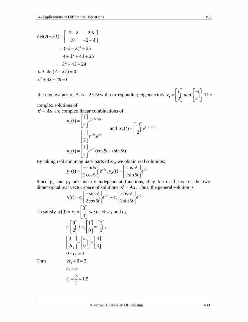
34-Applications to Differential Equations VU
©Virtual University Of Pakistan 439
2
2
2
2
2 2.5det( )
10 2
( 2 ) 254 4 25
4 29det( ) 04 29 0
A I
put A I
λλ
λ
λ
λ λ
λ λλ
λ λ
− − − − = − −
= − − +
= + + +
= + +− =
+ + =
the eigenvalues of A is 2 5i− ± with corresponding eigenvectors 2 2i i
and−
=
1v The
complex solutions of x Ax′ = are complex linear combinations of
( 2 5 )
2 5
( )2
.2
i t
t it
it e
ie e
− +
−
=
=
1x and ( 2 5 )( )
22x − −− =
i ti
t e
2( ) (cos5 sin 5 )21x −
= +
tit e t i t
By taking real and imaginary parts of x1, we obtain real solutions: 2 2sin 5 cos5
( ) , ( )2cos5 2sin 51 2y y− −−
= =
t tt tt e t e
t t
Since y1 and y2 are linearly independent functions, they form a basis for the two-dimensional real vector space of solutions x Ax′ = . Thus, the general solution is
2 21 2
sin 5 cos5( )
2cos5 2sin 5x − −−
= +
t tt tt c e c e
t t
To satisfy 0
3(0)
3x
= =
x we need sc1 and c2
Thus
1 2
2
1
2
1
2
1
0 1 3,
2 0 3
0 32 30
0 32 0 3
33 1.52
c c
ccc
cc
c
+ =
+ =
+ =+ =
=
= =

34-Applications to Differential Equations VU
©Virtual University Of Pakistan 440
2 2
1 2
2 2
2 2
2 2
2 2
2
sin 5 cos5( )
2cos5 2sin 5
sin 5 cos51.5 3
2cos5 2sin 5
1.5sin 5 3cos53cos5 6sin 5
1.5sin 5 3cos53cos5 6sin 5
t t
t t
t t
t t
t t
t
t tt c e c e
t t
t te e
t t
te tete te
te tete
− −
− −
− −
− −
− −
−
− = +
−
= +
−= +
− +=
+
x
2tte−
2( ) 1.5sin 5 3cos5( ) 3cos5 6sin 5
L t
C
i t t te
v t t t−− +
= +
Figure 5 The origin as a spiral point In this figure, due to the complex eigenvalues a rotation is caused by the sine and cosine function and hence the origin is called a spiral point. The trajectories spiral inwards as in this example the real part of the eigenvalue is negative. Similarly, it is important to note that when A has a complex eigenvalue with positive real part, the trajectories spiral outwards .And if the real part of the eigenvalue is zero, then the trajectories form ellipses around the origin.

34-Applications to Differential Equations VU
©Virtual University Of Pakistan 441
Exercise 1 The circuit in given figure can be described by
111 2 2 11
222 2 2 2
1 1 1 ( )( ) /( )( ) 1 1
( )
v tCR R R Cv tv t
v tR C R C
− +′ = ′ −
Where 1( )v t and 2 ( )v t are the voltages across the two capacitors at time t.
Suppose that resistor R1 is 1 ohms, R2 is 2 ohms, capacitor C1 is 1 farad, and capacitor C2 is 0.5 farad, and suppose that there is an initial charge of 7 volts on capacitor C1 and 6 volts on capacitor C2. Find formulas for v1(t) and v2(t) that describe how the voltages change over time. Exercise 2 Find formulas for the current Li and the voltage CV for the circuit in Example 4, assuming that 1 210 , 0.2 , 0.4 , 0.2R ohms R ohm C farad L henry= = = = the initial current is 0 amp, and the initial voltage is 16 volts.

35-Iterative Estimates for Eigenvalues VU
©Virtual University Of Pakistan 442
Lecture 35 Iterative Estimates for Eigenvalues
Eigenvalues and eigenvectors Let A be an n n× square matrix, λ is any scalar value. If there exists a non-zero vector X , such that it satisfies the equation AX Xλ= then λ is called the eigenvalue and X is called the corresponding eigenvector. i.e. if
00
( ) 0
AX XAX XAX IXA I X
λλλ
λ
=− =− =
− =
To find the eigenvalues we have to solve the equation 0A Iλ− = Example 1
Find the eigenvalues of1 01 2
A = −
.
Solution
1 01 2
1 0 1 0 1 0 0 1 01 2 0 1 1 2 0 1 2
A
A Iλ λ
λ λλ λ
= −
− − = − = − = − − − −
(1 )( 2 )A Iλ λ λ− = − − −
Solving 0A Iλ− = , we get (1 )( 2 ) 0λ λ− − − = So, either (1 ) 0λ− = or ( 2 ) 0λ− − = , 1 2so λ λ= = − are the eigenvalues of A. Power Method Let a matrix A is diagonalizable, with n linearly independent eigenvectors,
1 2, ,...n
v v v and corresponding eigenvalues 1 2, ,...
nλ λ λ such that
1 2 ...
nλ λ λ> ≥ ≥
Since 1 2{ , ,... }nv v v is a basis for nR , any vector x can be written as
1 1 2 2 ... n nx c v c v c v= + + +

35-Iterative Estimates for Eigenvalues VU
©Virtual University Of Pakistan 443
Multiplying both sides by A, we get 1 1 2 2
1 1 2 2
1 1 2 2
1 1 1 2 2 2
( ... )( ) ( ) .... ( )( ) ( ) ... ( )( ) ( ) ... ( )
n n
n n
n n
n n n
Ax A c v c v c vA c v A c v A c vc Av c Av c Avc v c v c vλ λ λ
= + + += + += + += + +
Again multiplying by A and simplifying as above, we get
2 2 2 21 1 1 2 2 2( ) ( ) ... ( )n n nA x c v c v c vλ λ λ= + +
Continuing this process we get
1 1 1 2 2 2
1 1 1 2 2 2
( ) ( ) ... ( )
( ) ( ) ) ... ( ) ( 1, 2,...)
k k k kn n n
k k k kn n n
A x c v c v c vA x c v c v c v k
λ λ λ
λ λ λ
= + +
= + + =
21 1 2 2
1 1 1
1( ) ( ) ) ... ( ) ( 1, 2,...)k k k knn nA x c v c v c v kλλ
λ λ λ= + + =
1 1 1( ) k kA x c vas kλ − →
→ ∞ Since
1 2 ...n
λ λ λ> ≥ ≥
Thus for large k, a scalar multiple of kA x determines almost the same direction as the eigenvector 1 1c v . Since, positive scalar multiples do not change the direction of the vector, kA x itself points almost in the same direction as 1v or 1v− , provided 1 0c ≠ . Procedure for finding the Eigenvalues and Eigenvectors Power Method To compute the largest eigenvalue and the corresponding eigenvector of the system ( ) ( )A X Xλ= Where A is a real, symmetric or un-symmetric matrix, the power method is widely used in practice. Procedure Step 1: Choose the initial vector such that the largest element is unity. Step 2: The normalized vector
(0)v is pre-multiplied by the matrix A. Step 3: The resultant vector is again normalized. Step 4: This process of iteration is continued and the new normalized vector is repeatedly pre-multiplied by the matrix A until the required accuracy is obtained. At this point, the result looks like
( ) ( 1) ( )[ ]k k k
ku A v q v−= =

35-Iterative Estimates for Eigenvalues VU
©Virtual University Of Pakistan 444
Here, kq is the desired largest eigenvalue and ( )kv is the corresponding eigenvector.
Example 2
Let1.8 .80.2 1.2
A =
, 1
41
v =
and
0.51
X−
=
. Then A has Eigenvalues 2 and 1, and the
eigenspace for 1 2λ = is the line through 0 and 1v . For k=0, …, 8, compute kA x and construct the line through 0 and kA x . What happens as k increases? Solution The first three calculations are
1.8 0.8 0.5 0.10.2 1.2 1 1.1
1.8 0.8 0.1 0.7( )
0.2 1.2 1.1 1.3
1.8 0.8 0.7 2.3( )
0.2 1.2 1.3 1.7
− − = =
−
= = =
= = =
2
3 2
Ax
A x A Ax
A x A A x
Analogous calculations complete Table 1. Table 1 Iterates of a Vector k 0 1 2 3 4 5 6 7 8
Akx .51
−
0.1
1.1−
0.71.3
2.31.7
5.52.5
11.94.1
24.77.3
50.313.7
101.526.5
The vectors 2, , ,..., kx Ax A x A x are shown in Fig. 1. The other vectors are growing too long to display. However, line segments are drawn showing the directions of those vectors. In fact, the directions of the vectors are what we really want to see, not the vectors themselves. The lines seem to be approaching the line representing the eigenspaces spanned by v1. More precisely, the angle between the line (subspace) determined by kA x and the line (eigenspaces) determined by 1v goes to zero as .k → ∞

35-Iterative Estimates for Eigenvalues VU
©Virtual University Of Pakistan 445
Figure 1 Directions determined by x, Ax, A2x, …, A7x The vectors 1( ) kA x−kλ in (3) are scaled to make them converge to 1 1c v , provided 1 0c ≠ . We cannot scale kA x in this way because we do not know 1λ but we can scale each kA x to make its largest entry 1. It turns out that the resulting sequence { }kx will converge to a multiple of 1v whose largest entry is 1. Figure 2 shows the scaled sequence for Example 1. The eigenvalue 1λ can be estimated from the sequence{ }kx too. When kx is close to an eigenvector for 1λ the vector kAx is close to 1λ kx with each entry in kAx approximately
1λ times the corresponding entry in kx . Because the largest entry in kx is 1 the largest entry in kAx is close to 1λ .
Figure 2 Scaled multiples of 2 7, , ,...,x Ax A x A x .

35-Iterative Estimates for Eigenvalues VU
©Virtual University Of Pakistan 446
Steps for finding the eigenvalue and the eigenvector
1. Select an initial vector 0x whose largest entry is 1. 2. For k=0,1,….
a. Compute kAx b. Let kµ be an entry in kAx whose absolute value is as large as possible.
c. Compute 11( )k k
k
x Axµ+ =
3. For almost all choices of 0x , the sequence { }kµ approaches the dominant eigenvalue, and the sequence { }kx approaches a dominant eigenvector. Example 3
Apply the power method to 6 51 2
A =
with 0
01
x =
. Stop when 5k = , and estimate the
dominant eigenvalue and a corresponding eigenvector of A. Solution To begin, we calculate 0Ax and identify the largest entry 0µ in 0Ax .
0
6 5 0 5, 5
1 2 1 20Ax = = =
µ
Scale 0Ax by 01 µ to get 1x , compute 1Ax and identify the largest entry in 1Ax
0
5 11 12 .451 0x Ax
= = = µ
1
6 5 1 8, 8
1 2 .4 1.81Ax = = =
µ
Scale 1Ax by 11 µ to get x2, compute 2Ax , and identify the largest entry in 2Ax .
1
8 11 11.8 .22582 1x Ax
= = = µ
2
6 5 1 7.125, 7.125
1 2 .225 1.4502Ax = = =
µ
Scale 2Ax by 21 µ to get 3x , and so on. The results of MATLAB calculations for the first five iterations are arranged in the Table 2. The evidence from the Table 2 strongly suggests that { }kx approaches (1, .2) and { }kµ approaches 7. If so, then (1, .2) is an eigenvector and 7 is the dominant eigenvalue. This
is easily verified by computing 1 6 5 1 7 1
7.2 1 2 .2 1.4 .2
A = = = =

35-Iterative Estimates for Eigenvalues VU
©Virtual University Of Pakistan 447
TABLE 2 The Power Method for Example 2
k 0 1 2 3 4 5 kx 0
1
1.4
1
.225
1
.2035
1
.2005
1
.20007
kAx 52
8
1.8
7.1251.450
7.01751.4070
7.00251.4010
7.000361.40014
kµ 5 8 7.125 7.0175 7.0025 7.00036 Example 4 Find the first three iterations of the power method applied on the following matrices
0
1 1 0 02 4 2 00 1 2 1
use x =
Solution 1st Iteration
1 0
1 1 0 0 0 0 0 02 4 2 0 0 0 2 20 1 2 1 0 0 2 2
u x+ +
= Α = = + + = + +
Now, we normalize the resultant vector to get
1 1 1
0 02 2 12 1
u q x = = =
2nd Iteration
2 1
1 1 0 0 0 1 0 12 4 2 1 0 4 2 60 1 2 1 0 1 2 3
u x+ +
= Α = = + + = + +
Now, we normalize the resultant vector to get
2 2 2
11 66 6 13 1
2
u q x
= = =
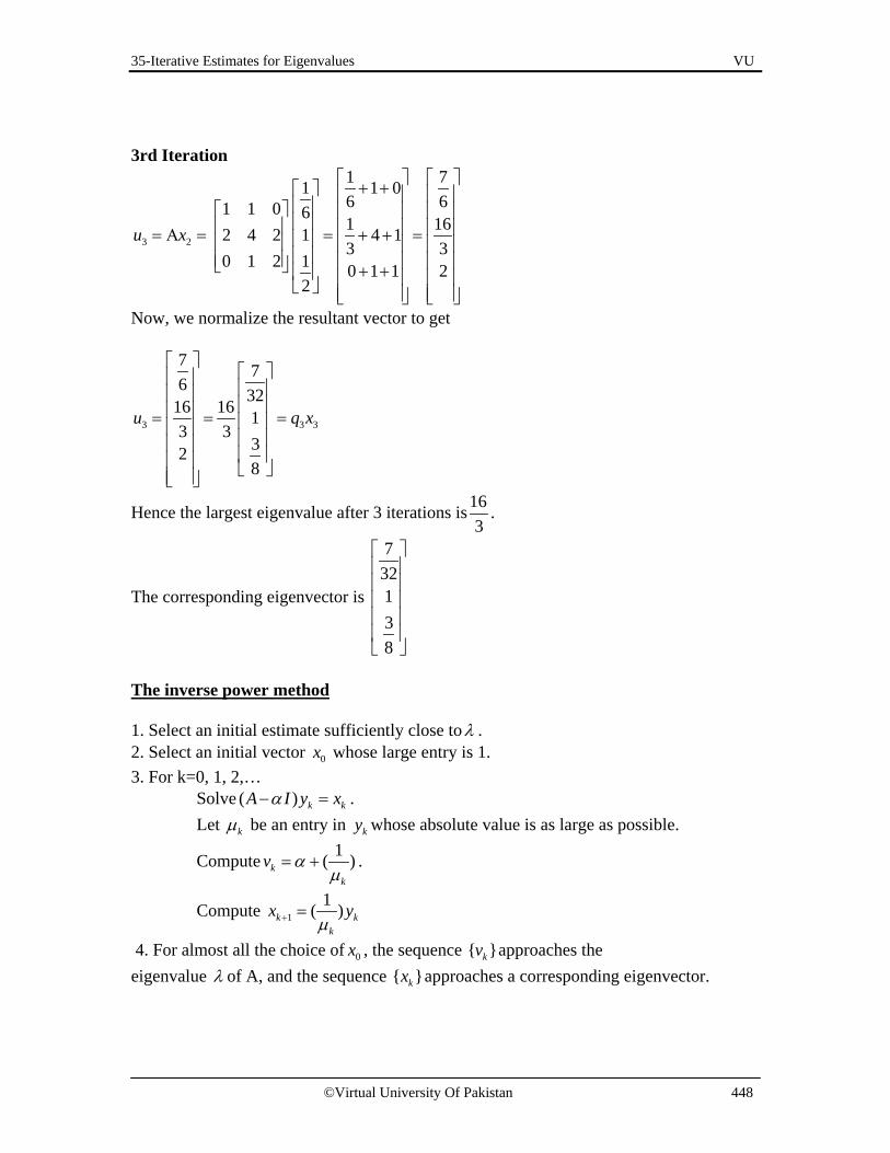
35-Iterative Estimates for Eigenvalues VU
©Virtual University Of Pakistan 448
3rd Iteration
3 2
1 71 1 06 61 1 0 6 1 162 4 2 1 4 13 3
0 1 2 1 0 1 1 22
u x
+ + = Α = = + + = + +
Now, we normalize the resultant vector to get
3 3 3
7 76 3216 16 13 3
328
u q x
= = =
Hence the largest eigenvalue after 3 iterations is163
.
The corresponding eigenvector is
732138
The inverse power method 1. Select an initial estimate sufficiently close to λ . 2. Select an initial vector 0x whose large entry is 1. 3. For k=0, 1, 2,… Solve ( ) k kA I y xα− = . Let kµ be an entry in ky whose absolute value is as large as possible.
Compute 1( )kk
v αµ
= + .
Compute 11( )k k
k
x yµ+ =
4. For almost all the choice of 0x , the sequence { }kv approaches the eigenvalue λ of A, and the sequence { }kx approaches a corresponding eigenvector.
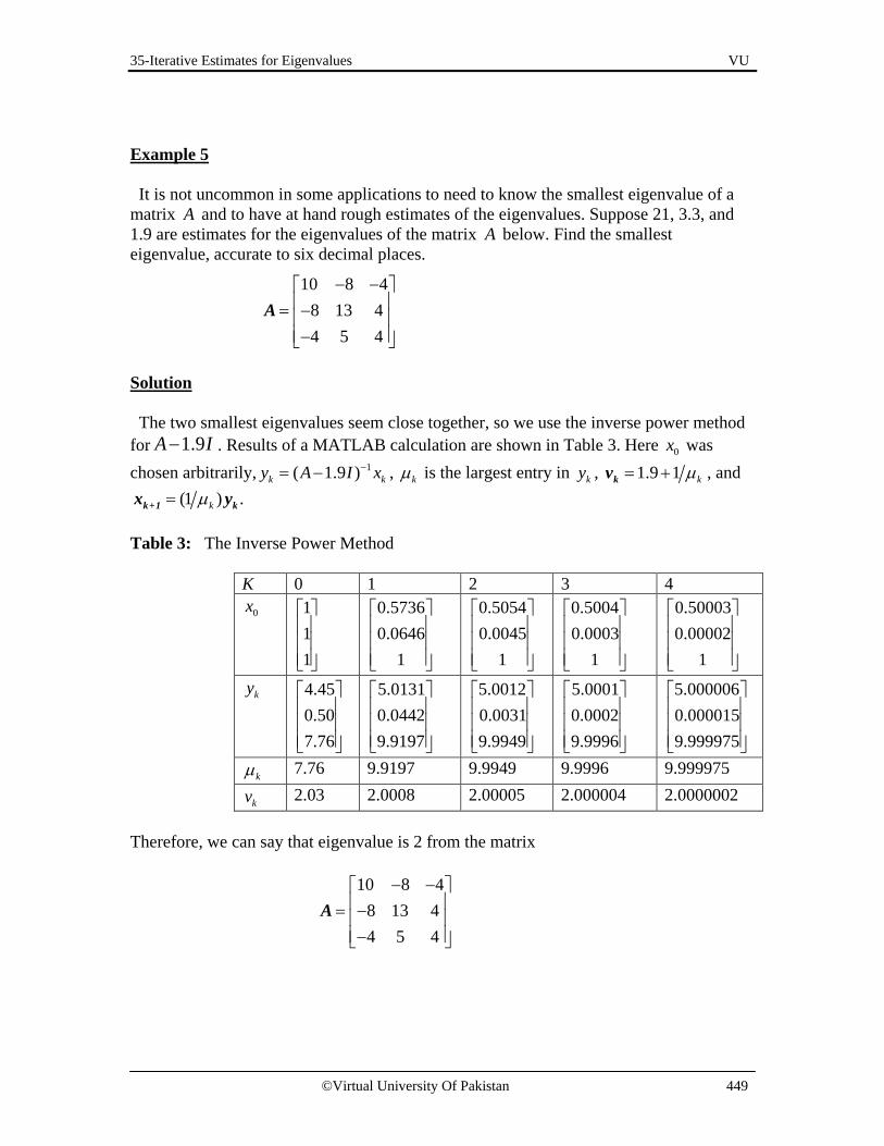
35-Iterative Estimates for Eigenvalues VU
©Virtual University Of Pakistan 449
Example 5 It is not uncommon in some applications to need to know the smallest eigenvalue of a matrix A and to have at hand rough estimates of the eigenvalues. Suppose 21, 3.3, and 1.9 are estimates for the eigenvalues of the matrix A below. Find the smallest eigenvalue, accurate to six decimal places.
Solution The two smallest eigenvalues seem close together, so we use the inverse power method for 1.9A I− . Results of a MATLAB calculation are shown in Table 3. Here 0x was chosen arbitrarily, 1( 1.9 )k ky A I x−= − , kµ is the largest entry in ky , 1.9 1kv = + kµ , and
(1 ) .k+1 kx y= kµ Table 3: The Inverse Power Method
K 0 1 2 3 4 0x 1
11
0.57360.0646
1
0.50540.0045
1
0.50040.0003
1
0.500030.00002
1
ky 4.450.507.76
5.01310.04429.9197
5.00120.00319.9949
5.00010.00029.9996
5.0000060.0000159.999975
kµ 7.76 9.9197 9.9949 9.9996 9.999975
kv 2.03 2.0008 2.00005 2.000004 2.0000002 Therefore, we can say that eigenvalue is 2 from the matrix
10 8 4
8 13 44 5 4
A− −
= − −
10 8 48 13 44 5 4
− − = − −
A

35-Iterative Estimates for Eigenvalues VU
©Virtual University Of Pakistan 450
Exercise How can you tell that if a given vector X is a good approximation to an eigenvector of a matrix A : if it is, how would you estimate the corresponding eigenvalue? Experiment with
5 8 48 3 14 1 2
A = − −
And 1.04.3
8.1X
= −
36- Revision VU
©Virtual University Of Pakistan 451
Lecture 36
Revision
Revision of Previous Lectures

37- Revision VU
©Virtual University Of Pakistan 452
Lecture 37
Revision
Revision of Previous Lectures

38- Inner Product VU
©Virtual University Of Pakistan 453
Lecture 38 Inner Product If u and v are vectors in nR , then we regard u and v as 1n× matrices. The transpose
tu is a 1 n× matrix, and the matrix product tu v is a 1 1× matrix which we write as a single real number (a scalar) without brackets. The number tu v is called the inner product of u and v . And often is written as .u v This inner product is also referred to as a dot product.
If
1
2
.
.
.
n
uu
u
u
=
and
1
2
.
.
.
n
vv
v
v
=
Then the inner product of u and v is
Example 1
Compute .u v and .v u when2 35 21 3
u and v = − = − −
.
Solution
2 35 21 3
u and v = − = − −
[ ]2 5 1tu = − −
[ ]3
. 2 5 1 2 2(3) ( 5)(2) ( 1)( 3)3
6 10 3 1
tu v u v = = − − = + − + − − −
= − + = −
1
2
1 2 1 1 2 2
.. . . ...
.
.
n n n
n
vv
u u u u v u v u v
v
= + + +

38- Inner Product VU
©Virtual University Of Pakistan 454
[ ]3 2 3tv = −
[ ]2
. 3 2 3 5 3(2) (2)( 5) ( 3)( 1)1
6 10 3 1
tv u v u = = − − = + − + − − −
= − + = −
Theorem Letu , v and w be vectors in nR , and let c be a scalar. Then
a. . .u v v u= b. ( ). . .u v w u w v w+ = + c. ( ). ( . ) .( )cu v c u v u cv= = d. . 0u u ≥ and . 0u u = if and only if 0u =
Observation
1 1 2 2
1 1 2 2
( .... ).
( . ) ( . ) ... ( . )p p
p p
c u c u c u wc u w c u w c u w
+ +
= + +
Length or Norm
The length or Norm of v is the nonnegative scalar v defined by 2 2 2
1 1
2
. ...
.nv v v v v v
v v v
= = + + +
=
Note: For any scalar c , cv c v=
Unit vector A vector whose length is 1 is called a unit vector. If we divide a non-zero vector v by its length v , we obtain a unit vector u as
vuv
=
The length of u is 1 1u vv
= =
Definition The process of creating the unit vector u from v is sometimes called normalizing v , and we say that u is in the same direction as v . In this case “u ” is called the normalized vector. Example 2 Let (1,2,2,0)v = in 4R . Find a unit vector u in the same direction as v . Solution The length of v is given by

38- Inner Product VU
©Virtual University Of Pakistan 455
2 2 2 21 2 3 4.v v v v v v v= = + + +
So, 2 2 2 21 2 2 0 1 4 4 0 9 3v = + + + = + + + = =
The unit vector u in the direction of v is given as
131
221 1 323
20 3
0
u vv
= = =
To check that 1u =
2 2 2 21 2 2 1 4 4. ( ) ( ) ( ) (0) 0 13 3 3 9 9 9
u u u −= = + + + = + + + =
Example 3
Let W be the subspace of 2R spanned by 2( ,1)3
X = . Find a unit vector Z that is a basis
for W. Solution W consists of all multiples of x, as in Fig. 2(a). Any nonzero vector in W is a basis for W. To simplify the calculation, x is scaled to eliminate fractions. That is, multiply x by 3 to get
23
y =
Now compute 2 2 22 3 13, 13,y y= + = = and normalize y to get
2 2 131313 3 13
z
= =
See Fig. 2(b). Another unit vector is ( 2 13 , 3 13).− −

38- Inner Product VU
©Virtual University Of Pakistan 456
Figure 2 Normalizing a vector to produce a unit vector. Definition For u and v vectors in nR , the distance between u and v , written as dist (u , v ), is the length of the vectoru v− . That is
Example 4 Compute the distance between the vectors u = (7, 1) and v = (3, 2) Solution
7 3 7 3 41 2 1 2 1
u v−
− = − = = − −
dist (u , v ) = 2 2(4) ( 1) 16 1 17u v− = + − = + = Law of Parallelogram of vectors The vectors, u , v and u v− are shown in the fig. below. When the vector u v− is added to v , the result isu . Notice that the parallelogram in the fig. below shows that the distance from u to v is the same as the distance of u v− to o .
( , )dist u v u v= −

38- Inner Product VU
©Virtual University Of Pakistan 457
Example 5 If 1 2 3( , , )u u u u= and 1 2 3( , , )v v v v= , then
2 2 21 1 2 2 3 3
( , ) ( ).( )
( ) ( ) ( )
dist u v u v u v u v
u v u v u v
= − = − −
= − + − + −
Definition Two vectors in u and v in nR are orthogonal (to each other) if . 0u v = Note The zero vector is orthogonal to every vector in nR because 0 . 0t v = for all v in nR . The Pythagorean Theorem Two vectors u and v are orthogonal if and only if 2 2 2u v u v+ = + Orthogonal Complements The set of all vectors z that are orthogonal to w in W is called the orthogonal complement of W and is denoted by w⊥ Example 6 Let W be a plane through the origin in R3, and let L be the line through the origin and perpendicular to W. If z and w are nonzero, z is on L, and w is in W, then the line segment from 0 to z is perpendicular to the line segment from 0 to w; that is, z . w = 0. So each vector on L is orthogonal to every w in W. In fact, L consists of all vectors that are orthogonal to the w’s in W, and W consists of all vectors orthogonal to the z’s in L. That is,
L W ⊥= and W L⊥=

38- Inner Product VU
©Virtual University Of Pakistan 458
Remarks The following two facts aboutW ⊥ , with W a subspace of Rn, are needed later in the segment. (1) A vector x is in W ⊥ if and only if x is orthogonal to every vector in a set that spans W. (2) W ⊥ is a subspace of Rn. Theorem 3 Let A be m x n matrix. Then the orthogonal complement of the row space of A is the null space of A, and the orthogonal complement of the column space of A is the null space of AT: (Row ) Nul ,A A⊥ = (Col ) NulA A⊥ = T Proof The row-column rule for computing Ax shows that if x is in Nul A, then x is orthogonal to each row of A (with the rows treated as vectors in Rn). Since the rows of A span the row space, x is orthogonal to Row A. Conversely, if x is orthogonal to Row A, then x is certainly orthogonal to each row of A, and hence Ax = 0. This proves the first statement. The second statement follows from the first by replacing A with AT and using the fact that Col A = Row AT. Angles in R2 and R3 If u and v are nonzero vectors in either R2 or R3, then there is a nice connection between their inner product and the angle ϑ between the two line segments from the origin to the points identified with u and v. The formula is
cosu v u v⋅ = ϑ (2) To verify this formula for vectors in R2, consider the triangle shown in Fig. 7, with sides of length , ,u v and .u v− By the law of cosines,
2 2 2 2 cosu v u v u v− = + − ϑ which can be rearranged to produce
2 2 2
2 2 2 2 2 21 2 1 2 1 1 2 2 1 1 2 2
1cos2
1 ( ) ( )2
u v u v u v
u v
= + − −
= + + + − − − − = + = ⋅ u u v v u v u v u v u v
ϑ
(u1, u2) u u v− ϑ v (v1, v2)
Figure 7 The angle between two vectors.

38- Inner Product VU
©Virtual University Of Pakistan 459
Example 7 Find the angle between the vectors (1, 1, 2), (2,1,0)u v= − = Solution
. (1)(2) ( 1)(1) (2)(0) 2 1 0 1u v = + − + = − + = And
2 2 2
2 2 2
(1) ( 1) (2) 1 1 4 6
(2) (1) (0) 4 1 5
u
v
= + − + = + + =
= + + = + =
Angle between the two vectors is given by
cosϑ ⋅=
u vu v
Putting the values, we get
Exercises Q.1
Compute .u v and .v u when1 35 13 5
u and v−
= =
Q.2 Let (2,1,0,3)v = in 4R . Find a unit vector u in the direction opposite to that of v . Q.3
Let W be the subspace of 3R spanned by 1 3 5( , , )2 2 2
X = . Find a unit vector Z that is a
basis for W. Q.4 Compute the distance between the vectors u = (1, 5, 7) and v = (2, 3, 5). Q.5 Find the angle between the vectors (2,1,3), (1,0, 2)u v= = .
1
1 1cos5 30
1cos30
1cos 79.4830
θ
θ
θ − °
= =
=
= =
6

39-Orthogonal and Orthonormal Sets VU
© Virtual University Of Pakistan 460
Lecture No.39 Orthogonal and Orthonormal sets
Objectives The objectives of the lecture are to learn about:
• Orthogonal Set. • Orthogonal Basis. • Unique representation of a vector as a linear combination of Basis vectors. • Orthogonal Projection. • Decomposition of a vector into sum of two vectors. • Orthonormal Set. • Orthonormal Basis. • Some examples to verify the definitions and the statements of the theorems.
Orthogonal Set Let { }1 2, ,..., pS u u u= be the set of non-zero vectors in ,nR is said to be an orthogonal set if all vectors in S are mutually orthogonal. That is O S∉ and . , , 1, 2,..., .i ju u o i j i j p= ∀ ≠ = Example Show that { }1 2 3, ,S u u u= is an orthogonal set. Where
1 2
3 11 , 21 1
u u−
= =
and 3
122 .72
u
−
= −
Solution To show that S is orthogonal, we show that each vector in S is orthogonal to other. That is
. , , 1, 2,3.i ju u o i j i j= ∀ ≠ = For 1, 2i j= =
1 2
3 1. 1 . 2
1 13 2 1 0
u u−
=
=− + + =
Which implies 1u is orthogonal to 2.u

39-Orthogonal and Orthonormal Sets VU
© Virtual University Of Pakistan 461
For 1, 3i j= =
1 3
13 2
. 1 . 21 7
23 72
2 20.
u u
− = −
−= − +
=
Which implies 1u is orthogonal to 3.u For 2, 3i j= =
2 3
11 2
. 2 . 21 7
21 742 20.
u u
− − = −
= − +
=
Which implies 2u is orthogonal to 3.u
Thus { }1 2 3, ,S u u u= is an orthogonal set. Theorem Suppose that { }1 2, ,..., pS u u u= is an orthogonal set of non-zero vectors in nR and
{ }1 2, ,..., .pW Span u u u= Then S is linearly independent set and a basis for .W Proof Suppose
1 1 2 20 ... .p pc u c u c u= + + +
Where 1 2, ..., pc c c are scalars.
1 1 1 1 2 2
1 1 1 1 2 2 1
1 1 1 2 1 2 1
1 1 1
.0 .( ... )
0 .( ) .( ) ... .( )
( . ) ( . ) ... ( . )
( . )
p p
p p
p p
u u c u c u c uu c u u c u u c uc u u c u u c u uc u u
= + + +
= + + +
= + + +
=

39-Orthogonal and Orthonormal Sets VU
© Virtual University Of Pakistan 462
Since S is orthogonal set, so, 1 2 1. ... . 0pu u u u+ + = but 1 1. 0.u u >
Therefore 1 0c = . Similarly, it can be shown that 2 3 ... 0pc c c= = = =
Therefore by definition { }1 2, ,..., pS u u u= is linearly independent set and by definition of basis is a basis for subspaceW . Example If { }1 2,S u u= is an orthogonal set of non-zero vector in 2R . Show that S is linearly independent set. Where
1
31
u =
and 2
1.
3u
− =
Solution To show that { }1 2,S u u= is linearly independent set, we show that the following vector equation
1 1 2 2 0.c u c u+ = has only the trivial solution. i.e. 1 2 0.c c= =
1 1 2 2
1 2
1 2
1 2
1 2
1 2
0
3 1 01 3 0
3 03 0
3 0
3 0
c u c u
c c
c c
c c
c c
c c
+ =
−+ =
−+ =
− =
+ =
Solve them simultaneously, gives 1 2 0.c c= =
Therefore if S is an orthogonal set then it is linearly independent. Orthogonal basis Let { }1 2, ,..., pS u u u= be a basis for a subspace W of ,nR is also an orthogonal basis if S is an orthogonal set. Theorem If { }1 2, ,..., pS u u u= is an orthogonal basis for a subspace W of nR . Then each y in W can
be uniquely expressed as a linear combination of 1 2, ,..., .pu u u That is
1 1 2 2 ... .p py c u c u c u= + + +

39-Orthogonal and Orthonormal Sets VU
© Virtual University Of Pakistan 463
Where ..
jj
j j
y uc
u u=
Proof
1 1 1 2 2 1
1 1 1 2 2 1 1
1 1 1 2 1 2 1
1 1 1
. ( ... ).
( ). ( ). ... ( ).
( . ) ( . ) ... ( . )
( . ).
p p
p p
p p
y u c u c u c u uc u u c u u c u u
c u u c u u c u uc u u
= + + +
= + + +
= + + +
=
Since S is orthogonal set, so, 1 2 1. ... . 0pu u u u+ + = but 1 1. 0.u u > Hence
11
1 1
..
y ucu u
= and similarly 22
2 2
.. ,... .. .
pp
p p
y uy uc cu u u u
= =
Example The set { }1 2 3, ,S u u u= as in first example is an orthogonal basis for 3R . Express y as a linear combination of the vectors in .S Where
[ ]6 1 8 Ty = − Solution We want to write
1 1 2 2 3 3y c u c u c u= + + Where 1 2,c c and 3c are to be determined. By the above theorem
11
1 1
..
y ucu u
=
6 31 . 18 1 11 13 3 111 . 11 1
− = = =

39-Orthogonal and Orthonormal Sets VU
© Virtual University Of Pakistan 464
22
2 2
..
6 11 . 28 1 12 21 1 62 . 21 1
y ucu u
=
− − − = = = −− −
And 3
33 3
..
16 21 . 28 7
332 21 1 33/ 2
2 22 . 27 72 2
y ucu u
=
− − − − = = = −
− − − −
Hence 1 2 32 2y u u u= − − .
Example The set { }1 2 3, ,S u u u= is an orthogonal basis for 3R . Write y as a linear combination of the vectors in .S Where
1 2
3 1 17 , 1 , 14 0 0
y u u = = − =
and 3
001
u =
Solution We want to write
1 1 2 2 3 3y c u c u c u= + +

39-Orthogonal and Orthonormal Sets VU
© Virtual University Of Pakistan 465
Where 1 2,c c and 3c are to be determined. By the above theorem
11
1 1
3 17 . 14 0. 3 7 0 21 1. 1 1 01 . 10 0
y ucu u
− − + = = = =−
+ + − −
22
2 2
3 17 . 14 0. 3 7 0 51 1. 1 11 . 10 0
y ucu u
+ + = = = =
+
And
33
3 3
3 07 . 04 1. 4 40 0. 10 . 01 1
y ucu u
= = = =
Hence 1 2 32 5 4y u u u=− + + .
Exercise The set { }1 2 3, ,S u u u= is an orthogonal basis for 3R . Write y as a linear combination of the vectors in .S where
1 2
152 221 , 1 ,5
3 0 1
y u u
= = − = −
and 3
83
16383
u
=

39-Orthogonal and Orthonormal Sets VU
© Virtual University Of Pakistan 466
An Orthogonal Projection (Decomposition of a vector into the sum of two vectors Decomposition of a non- zero vector y nR∈ into the sum of two vectors in such a way, one is multiple of u nR∈ and the other orthogonal tou . That is
y y z∧= +
Where y uα∧ = for some scalar α and z is orthogonal tou .
y∧− z y y∧= − u y y uα∧ = z y y∧= − y∧− In the above figure a vector y is decomposed into two vectors z y y∧= − and .y uα∧ = Clearly it can be seen that z y y∧= − is orthogonal to u and y uα∧ = is a multiple ofu . Since z y y∧= − is orthogonal to u. Therefore
. 0( ). 0( ). 0
. ( . ) 0..
z uy y uy u u
y u u uy uu u
αα
α
∧
=
− =− =− =
⇒ =
And
.
.
z y yy uy uu u
∧= −
= −

39-Orthogonal and Orthonormal Sets VU
© Virtual University Of Pakistan 467
Hence
..
y uy uu u
∧ = , which is an orthogonal projection of y ontou .
And
.
.
z y yy uy uu u
∧= −
= − is a component of y
Example
Let 76
=
y and 42
=
u .
Find the orthogonal projection of y onto u. Then write y as a sum of two orthogonal vectors, one in span {u} and one orthogonal to u. Solution Compute
7 440
6 2
4 420
2 2
y u
u u
⋅ = ⋅ =
⋅ = ⋅ =
The orthogonal projection of y onto u is 4 840ˆ 22 420
y uy u uu u
⋅= = = = ⋅
and the
component of y orthogonal to u is 7 8 1
ˆ6 4 2
y y−
− = − =
The sum of these two vectors is y. That is, 7 8 16 4 2
ˆ ˆ( )y y y y
− = +
−
This decomposition of y is illustrated in Fig. 3. Note: If the calculations above are correct, then ˆ ˆ{ , }y y y− will be an orthogonal set. As a check, compute
8 1ˆ ˆ( ) 8 8 0
4 2y y y
− ⋅ − = ⋅ = − + =

39-Orthogonal and Orthonormal Sets VU
© Virtual University Of Pakistan 468
x2 •y L = Span {u} ˆy y− • y • 2 •u x1 1 8
Figure 3 The orthogonal projection of y on to a line through the origin. Example Find the distance in figure below from y to L. x2 •y L = Span {u} ˆy y− • y • 2 •u x1 1 8 Solution The distance from y to L is the length of the perpendicular line segment from y to the
orthogonal projection y . The length equals the length of ˆy y− . This distance is
2 2ˆ ( 1) 2 5y y− = − + =

39-Orthogonal and Orthonormal Sets VU
© Virtual University Of Pakistan 469
Example Decompose y = (-3,-4) into two vectors y and z, where y is a multiple of u = (-3, 1) and z is orthogonal to u. Also prove that . 0y z∧ = Solution It is very much clear that y∧ is an orthogonal projection of y onto u and it is calculated by applying the following formula
.
.y uy uu u
∧ =
3 3.
34 13 3 1
.1 1
− − −− = − −
39 419 1− −
= +
3112−
=
3212
− =
33 3 3/ 23 24 4 1/ 2 92
212
z y y∧
− − − + − = − = − = = − − − −
So, 3 32 21 92 2
y and z∧
− − = = −
Now

39-Orthogonal and Orthonormal Sets VU
© Virtual University Of Pakistan 470
3 32 2. .1 92 2
9 94 40
y z∧
− − = −
= −
=
Therefore, y∧ is orthogonal to z Exercise Find the orthogonal projection of a vector y = (-3, 2) onto u = (2, 1). Also prove that y y z∧= + , where y∧ a multiple of u and z is is an orthogonal to u. Orthonormal Set Let { }1 2, ,..., pS u u u= be the set of non-zero vectors in ,nR is said to be an orthonormal set if S is an orthogonal set of unit vectors. Example Show that { }1 2 3, ,S u u u= is an orthonormal set. Where
1 2
205
0 , 11 05
u u
= = − −
and 3
15
0 .25
u
=
Solution To show that S is an orthonormal set, we show that it is an orthogonal set of unit vectors. It can be easily prove that S is an orthogonal set because
. 0 , , 1, 2,3.i ju u i j i j= ∀ ≠ = Furthermore

39-Orthogonal and Orthonormal Sets VU
© Virtual University Of Pakistan 471
1 2 3
1 1
2 2
2 105 5
0 , 1 0 .1 0 25 5
2 25 5
. 0 . 01 15 5
4 105 5
10 0
. 1 . 10 0
0 1 01
u u u
u u
u u
= = − = −
= − −
= + +
=
= − −
= + +=
And
3 3
1 15 5
. 0 . 02 25 5
1 45 51
u u
=
= +
=
Hence { }1 2 3, ,S u u u= is an orthonormal set.
Orthonormal basis Let { }1 2, ,..., pS u u u= be a basis for a subspace W of ,nR is also an orthonormal basis if S is an orthonormal set. Example

39-Orthogonal and Orthonormal Sets VU
© Virtual University Of Pakistan 472
Show that { }1 2 3, ,S u u u= is an orthonormal basis of 3,R where
1 2
13
611 21 , 611 11
611
u u
− = =
and 3
1664 .66766
u
−
− =
Solution To show that { }1 2 3, ,S u u u= is an orthonormal basis, it is sufficient to show that it is an orthogonal set of unit vectors. That is
. 0 , , 1, 2,3.i ju u i j i j= ∀ ≠ = And
. 1 , , 1, 2,3.i ju u i j i j= ∀ = = Clearly it can be seen that
1 2
1 3
. 0,
. 0u uu u
==
And 2 3. 0.u u =
Furthermore 1 1
2 2
. 1,. 1
u uu u
==
And 3 3. 1.u u =
Hence S is an orthonormal basis of 3.R Theorem A m n× matrix U has orthonormal columns if and only if tU U I= Proof Keep in mind that in an if and only if statement, one part depends on the other, so, each part is proved separately. That is, we consider one part and then prove the other part with the help of that assumed part. Before proving both sides of the statements, we have to do some extra work which is necessary for the better understanding. Let 1 2, ,..., mu u u be the columns of U. Then U can be written in matrix form as [ ]1 2 3 ... mU u u u u= Taking transpose, it becomes

39-Orthogonal and Orthonormal Sets VU
© Virtual University Of Pakistan 473
1
2
3
.
.
.
t
t
t
t
tm
uuu
U
u
=
[ ]
1
2
3
1 2 3. . . ...
t
t
t
tm
tm
uuu
U U u u u u
u
=
1 1 1 2 1 3 1
2 1 2 2 2 3 2
3 1 3 2 3 3 3
1 2 3
...
...
.... . . .. . . .. . . .
...
t t t tm
t t t tm
t t t tm
t t t tm m m m m
u u u u u u u uu u u u u u u uu u u u u u u u
u u u u u u u u
=
1 1 1 2 1 3 1
2 1 2 2 2 3 2
3 1 3 2 3 3 3
1 2 3
.
. . . ... .. . . ... .. . . ... .
. . . .
. . . .
. . . .. . . ... .
t
m
m
mt
m m m m m
As u v v uTherefore
u u u u u u u uu u u u u u u uu u u u u u u u
U U
u u u u u u u u
=
=
Now, we come to prove the theorem. First suppose that ,tU U I= and we prove that columns of U are orthonormal. Since, we assume that

39-Orthogonal and Orthonormal Sets VU
© Virtual University Of Pakistan 474
1 1 1 2 1 3 1
2 1 2 2 2 3 2
3 1 3 2 3 3 3
1 2 3
. . . ... .. . . ... .. . . ... .
. . . .
. . . .
. . . .. . . ... .
1 0 0 ... 00 1 0 ... 00 0 1 ... 0. . . .. . . .. . . .0 0 0 ... 1
m
m
mt
m m m m m
u u u u u u u uu u u u u u u uu u u u u u u u
U U
u u u u u u u u
= =
Clearly, it can be seen that
. 0 , 1, 2,...
. 1 , 1, 2,...
i j
i j
u u for i j i j mandu u for i j i j m
= ≠ =
= = =
Therefore, columns of U are orthonormal. Next suppose that the columns of U are orthonormal and we will show that .tU U I= Since we assume that columns of U are orthonormal, so, we can write
. 0 , 1, 2,...
. 1 , 1, 2,...
i j
i j
u u for i j i j mandu u for i j i j m
= ≠ =
= = =
Hence,
1 1 1 2 1 3 1
2 1 2 2 2 3 2
3 1 3 2 3 3 3
1 2 3
. . . ... .. . . ... .. . . ... .
. . . .
. . . .
. . . .. . . ... .
m
m
mt
m m m m m
u u u u u u u uu u u u u u u uu u u u u u u u
U U
u u u u u u u u
=

39-Orthogonal and Orthonormal Sets VU
© Virtual University Of Pakistan 475
1 0 0 ... 00 1 0 ... 00 0 1 ... 0. . . .. . . .. . . .0 0 0 ... 1
=
That is
.tU U I= Which is our required result. Exercise Prove that the following matrices have orthonormal columns using above theorem.
1 11(1)1 12
2 2 1(2) 1 2 2
2 1 2
cos sin(3)
sin cosθ θθ θ
−
− − −
Solution (1) Let
1 111 121 111 12
1 1 1 111 1 1 121 00 1
t
t
t
U
U
Then
U U
I
U U I
= −
= −
= − −
= =
=
Therefore, by the above theorem, U has orthonormal columns. (2) And (3) are left for reader.
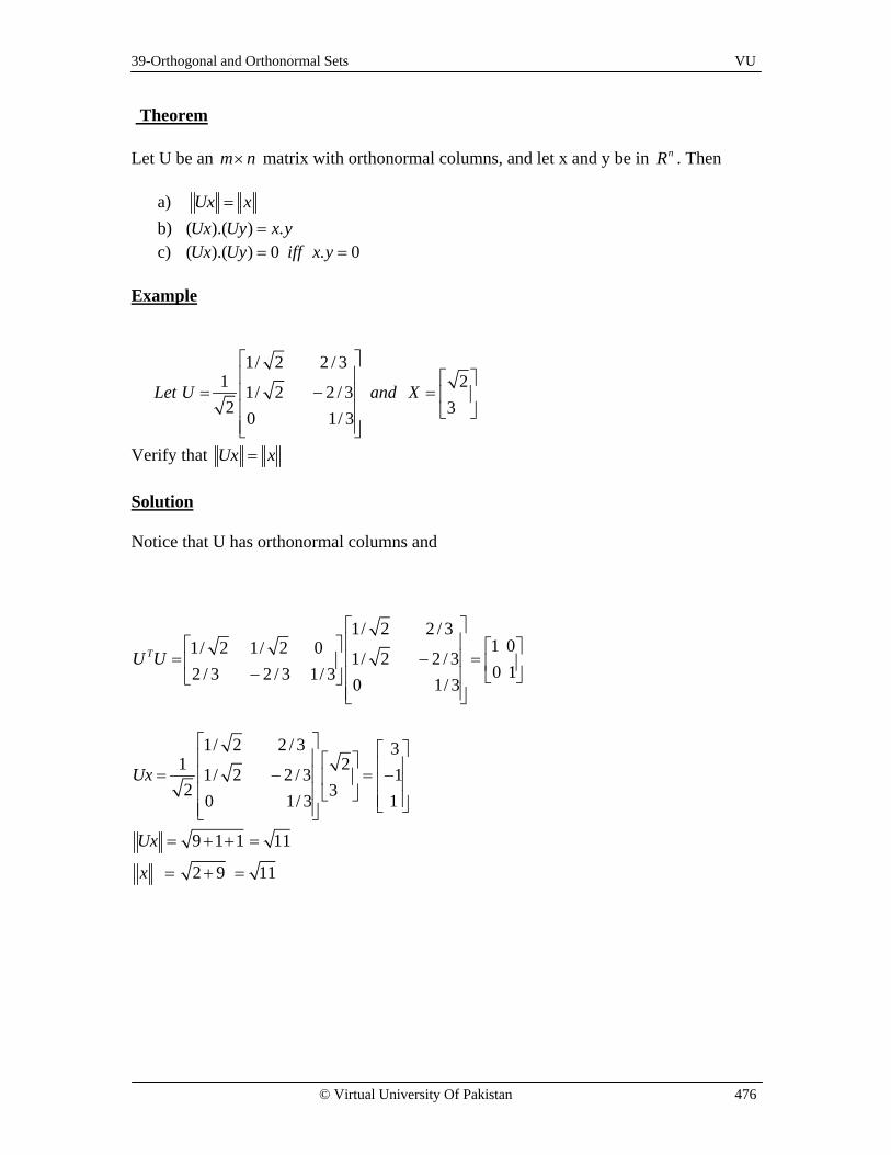
39-Orthogonal and Orthonormal Sets VU
© Virtual University Of Pakistan 476
Theorem Let U be an m n× matrix with orthonormal columns, and let x and y be in nR . Then
a) Ux x= b) ( ).( ) .Ux Uy x y= c) ( ).( ) 0 . 0Ux Uy iff x y= =
Example
1/ 2 2 / 31 21/ 2 2 / 32 30 1/ 3
Let U and X
= − =
Verify that Ux x= Solution Notice that U has orthonormal columns and
1/ 2 2 / 31 01/ 2 1/ 2 0 1/ 2 2 / 30 12 / 3 2 / 3 1/ 3 0 1/ 3
TU U
= − = −
1/ 2 2 / 3 3
1 21/ 2 2 / 3 12 30 1/ 3 1
9 1 1 11
2 9 11
Ux
Ux
x
= − = −
= + + =
= + =

40-Orthogonal Decomposition VU
©Virtual University Of Pakistan 477
Lecture No.40
Orthogonal Decomposition Objectives The objectives of the lecture are to learn about:
• Orthogonal Decomposition Theorem. • Best Approximation Theorem.
Orthogonal Projection The orthogonal projection of a point in 2R onto a line through the origin has an important analogue in nR . That is given a vector Y and a subspace W in nR , there is a vector y in W such that 1) y is the unique vector in W for which ˆy y− is orthogonal to W, and 2) y is the unique vector in W closest to y. y 0 y We observe that whenever a vector y is written as a linear combination of vectors
1 2, , ..., nu u u in a basis of nR , the terms in the sum for y can be grouped into two parts so that y can be written as 1 2y z z= + , where 1z is a linear combination of some of the iu ’s, and 2z is a linear combination of the rest of the 'iu s . This idea is particularly useful when { }1 2, , ..., nu u u is an orthogonal basis.
Example 1 Let { }1 2 5, , ...,u u u be an orthogonal basis for 5R and let 1 2 5 5...y c c c= + + +1 2u u u . Consider the subspace W= Span{u1, u2} and write y as the sum of a vector 1z in W and a vector 2z in ⊥W . Solution
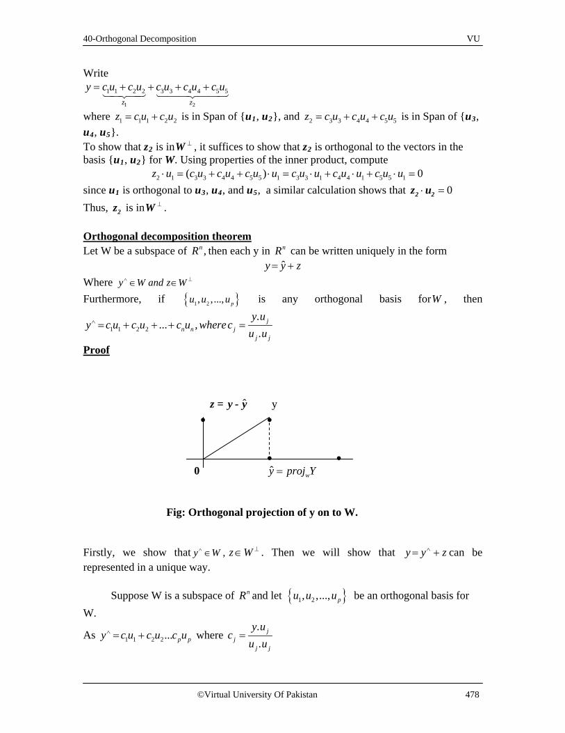
40-Orthogonal Decomposition VU
©Virtual University Of Pakistan 478
Write
1 2
1 1 2 2 3 3 4 4 5 5
z z
y c u c u c u c u c u= + + + +
where 1 1 1 2 2z c u c u= + is in Span of {u1, u2}, and 2 3 3 4 4 5 5z c u c u c u= + + is in Span of {u3, u4, u5}. To show that z2 is in ⊥W , it suffices to show that z2 is orthogonal to the vectors in the basis {u1, u2} for W. Using properties of the inner product, compute
2 1 3 3 4 4 5 5 1 3 3 1 4 4 1 5 5 1( ) 0z u c u c u c u u c u u c u u c u u⋅ = + + ⋅ = ⋅ + ⋅ + ⋅ = since u1 is orthogonal to u3, u4, and u5, a similar calculation shows that 0⋅ =2 2z u Thus, 2z is in ⊥W . Orthogonal decomposition theorem Let W be a subspace of ,nR then each y in nR can be written uniquely in the form
ˆy y z= + Where y W and z W∧ ⊥∈ ∈ Furthermore, if { }1 2, , ..., pu u u is any orthogonal basis forW , then
1 1 2 2
.... ,
.j
n n jj j
y uy c u c u c u wherec
u u∧ = + + + =
Proof ˆz = y - y y • • • • 0 ˆ wy proj Y= Fig: Orthogonal projection of y on to W. Firstly, we show that ,y W∧ ∈ z W ⊥∈ . Then we will show that y y z∧= + can be represented in a unique way. Suppose W is a subspace of nR and let { }1 2, ,..., pu u u be an orthogonal basis for W.
As 1 1 2 2... p py c u c u c u∧ = + where ..
jj
j j
y uc
u u=
40-Orthogonal Decomposition VU
©Virtual University Of Pakistan 479
Since { }1 2, ,..., pu u u is the basis for W and y∧ is written as a linear combination of
these basis vectors. Therefore, by definition of basis .y W∧ ∈ Now, we will show that z y y W∧ ⊥= − ∈ . For this it is sufficient to show that jz u⊥ for each 1,2,... .j p= Let 1u W∈ be an arbitrary vector.
1 1
1 1
1 1 1 2 2 1
1 1 1 1 2 2 1 1
1 1 1 1 1
11 1 1
1 1
1 1
. ( ).
. .. ( ... ).
. ( . ) ( . ) ... ( . )
. ( . ) . 0, 2,3,...
.. ( . ).
. .0
p p
p p
j
z u y y uy u y uy u c u c u c u uy u c u u c u u c u uy u c u u where u u j p
y uy u u uu u
y u y u
∧
∧
= −
= −= − + + +
= − − −
= − = =
= −
= −=
Therefore, 1.z u⊥ Since 1u is an arbitrary vector, therefore jz u⊥ for 1, 2,... .j p=
Hence by definition of ,W z W⊥ ⊥∈ Now, we must show that y y z∧= + is unique by contradiction. Let y y z∧= + and 1 1,y y z∧= + where 1,y y W∧ ∧ ∈ and 1, ,z z W ⊥∈ also 1 1z z and y y∧ ∧≠ ≠ . Since above representations for y are equal, that is
1 1
1 1
y z y zy y z z
∧ ∧
∧ ∧
+ = +
⇒ − = −
Let 1s y y∧ ∧= −
Then 1s z z= −
Since W is a subspace, therefore, by closure property 1s y y W∧ ∧= − ∈
Furthermore, W ⊥ is also a subspace, therefore by closure property 1s z z w⊥= − ∈
Since s W∈ and .s W ⊥∈ Therefore by definition s s⊥ That is s. s=0 Therefore
1
1
0s y yy y
∧ ∧
∧ ∧
= − =
⇒ =

40-Orthogonal Decomposition VU
©Virtual University Of Pakistan 480
Also 1z z=
This shows that representation is unique. Example
Let 1
251
u = −
, 2
211
u− =
, and 123
y =
Observe that { }1 2,u u is an orthogonal basis for W=span{ }1 2,u u , write y as the sum of a vector in W and a vector orthogonal to W. Solution Since ,y W∧ ∈ therefore y∧ can be written as following:
1 1 2 2
1 21 2
1 1 2 2
. .. .
2 2 2 29 3 9 155 1 5 130 6 30 30
1 1 1 1
2 / 5 212 105
1/ 5 1
y c u c uy u y uu uu u u u
∧ = +
= +
− − = + = + − − − −
= =
1 2 / 5 7 / 52 2 03 1/ 5 14 / 5
17 / 5 0
2
y y∧
− − = − =
=
Above theorem ensures that y y∧− is in W ⊥ . You can also verify by 1( ). 0y y u∧− = and 2( ). 0y y u∧− = . The desired decomposition of y is

40-Orthogonal Decomposition VU
©Virtual University Of Pakistan 481
1 2 / 5 7 / 52 2 03 1/ 5 14 / 5
y−
= = +
Example
Let W=span{ }1 2,u u , where 1
132
u = −
and 2
421
u =
Decompose 225
y = −
into two vectors; one in W and one in .W ⊥ Also verify that these
two vectors are orthogonal. Solution Let y W∧ ∈ and .z y y W∧ ⊥= − ∈ Since ,y W∧ ∈ therefore y∧ can be written as following:
1 1 2 2
1 21 2
1 1 2 2
. .. .
1 49 33 27 7
2 1
333
y c u c uy u y uu uu u u u
y
∧
∧
= +
= +
= − + = −
Now 2 32 35 3
112
z y y
z
∧
= − = − − − − =
Now we show that ,z y∧⊥ i.e. . 0z y∧ =
40-Orthogonal Decomposition VU
©Virtual University Of Pakistan 482
1 3. 1 . 3
2 30
z y∧
− = −
=
Therefore .z y∧⊥ Exercise
Let W=span{ }1 2,u u , where 1
103
u = −
and 2
311
u =
Write 6
812
y = −
as a sum of two vectors; one in W and one in .W ⊥ Also verify that these
two vectors are orthogonal. Best Approximation Theorem Let W is a finite dimensional subspace of an inner product space V and y is any vector in V. The best approximation to y from W is then Pr y
woj , i.e for every w (that is not Pr y
woj ) in W, we have
Pr .ywy oj y w− < −
Example
Let W=span{ }1 2,u u , where 1
132
u = −
, 2
421
u =
and225
y = −
. Then using above
theorem, find the distance from y to W. Solution Using above theorem the distance from y to W is calculated using the following formula
Pr ywy oj y y∧− = −
Since, we have already calculated 2 3 12 3 15 3 2
y y∧
− − = − − − =
So 6y y∧− = Example
40-Orthogonal Decomposition VU
©Virtual University Of Pakistan 483
The distance from a point y in nR to a subspace W is defined as the distance from y to the nearest point in W. Find the distance from y to W =span{ }1 2,u u , where
1 2
1 5 15 , 2 , 2
10 1 1y u u
− = − = − = −
By the Best Approximation Theorem, the distance from y to W is ˆ ,y y− where y = projwy. Since, {u1, u2} is an orthogonal basis for W, we have
1 2
5 1 115 21 1 7ˆ 2 2 830 6 2 2
1 1 4y u u
− − = + = − − = −
−
1 1 0ˆ 5 8 3
10 4 6
− − − = − − − =
y y
2 2 2ˆ 3 6 45y y− = + =
The distance from y to W is 45 3 5.= Theorem If { }1 2, ,..., pu u u is an orthonormal basis for a subspace W of nR , then
1 1 2 2
1 2
Pr ( . ) ( . ) ...( . )
[ .... ]
Pr
w p p
p
y T nw
oj y y u u y u u y u uIf U u u u
then oj UU y y in R
= + +
=
= ∀
Example
Let 1 2
7 1 91 , 1 , 14 2 6
u u y− − − = = = −
and W =span{ }1 2,u u . Use the fact that u1 and u2 are orthogonal to compute Pr woj y . Solution

40-Orthogonal Decomposition VU
©Virtual University Of Pakistan 484
1 21 2
1 1 2 2
1 2
. .Pr. .
88 266 6
7 1 94 11 1 13 3
4 2 6
wy u y uoj y u uu u u u
u u
y
= +
−= +
− − − = − = =
In this case,y happens to be a linear combination of u1 and u2 . So y is in W. The closest point in W to y is y itself.

41-Othogonal basis, Gram-Schmidt process, Orthonormal basis VU
©Virtual University Of Pakistan 485
Lecture # 41
Orthogonal basis, Gram-Schmidt Process, Orthonormal basis
Example 1 Let W = Span {x1, x2}, where
1 2
3 16 20 2
x and x = =
Find the orthogonal basis {v1, v2} for W.
Solution
Let P be a projection of x2 on to x1. The component of x2 orthogonal to x1 is x2 – P, which is in W as it is formed from x2 and a multiple of x1.
Let v1 = x1 and compute
Thus, {v1, v2} is an orthogonal set of nonzero vectors in W , dim W = 2 and {v1, v2} is a basis of W.
Example 2 For the given basis of a subspace W = Span {x1, x2},
1 2
0 54 62 7
x and x = = −
Find the orthogonal basis {v1, v2} for W.
Solution Set v1 = x1 and compute
2 12 2 2 1
1 1
1 3 0. 15 2 6 0. 45
2 0 2
x vv x P x vv v
= − = − = − =

41-Othogonal basis, Gram-Schmidt process, Orthonormal basis VU
©Virtual University Of Pakistan 486
Thus, an orthogonal basis for W is 0 54 , 42 8
−
Theorem Given a basis {x1, …, xp} for a subspace W of nR . Define
Then {v1, …,vp} is an orthogonal basis for W. In addition Span {v1, …, vk}= Span {x1,…, xk} for 1 k p≤ ≤
Example 3
The following vectors {x1, x2, x3} are linearly independent
1 2 3
1 0 01 1 0
, ,1 1 11 1 1
x x x
= = =
Construct an orthogonal basis for W by Gram-Schmidt Process.
2 12 2 1
1 1
5 0. 10 6 4. 20
-7 2
5 0 516 4 42
-7 2 8
x vv x vv v
= − = −
= − = −
2 11 1 2 2 1
1 1
3 1 3 23 3 1 2
1 1 2 2
1 2 -11 2 -1
1 1 2 2 -1 -1
..
. .. .
. . ....
. . .p p p p
p p pp p
x vv x v x vv v
x v x vv x v vv v v v
x v x v x vv x v v v
v v v v v v
= = −
= − −
= − − − −

41-Othogonal basis, Gram-Schmidt process, Orthonormal basis VU
©Virtual University Of Pakistan 487
Solution
To construct orthogonal basis we have to perform the following steps.
Step 1 Let v1 = x1
Step 2
Let 2 12 2 1
1 1
. .
x vv x vv v
= −
Since
0 1 3 / 4 31 1 1/ 4 131 1 1/ 4 141 1 1/ 4 1
− − = = − = =
2 1v x
Step 3
3 1 3 23 3 1 2
1 1 2 2
0 1 3 00 1 1 2 / 3. . 2 21 1 1 2 / 3. . 4 121 1 1 2 / 3
x v x vv x v vv v v v
− = − + = − + =
Thus, {v1, v2, v3} is an orthogonal set of nonzero vectors in W.
Example 4
Find an orthogonal basis for the column space of the following matrix by Gram-Schmidt Process.
3
0 0 00 2 / 3 2 / 31 2 / 3 1/ 31 2 / 3 1/ 3
v
− = − =

41-Othogonal basis, Gram-Schmidt process, Orthonormal basis VU
©Virtual University Of Pakistan 488
1 6 63 8 31 2 61 4 3
− − − − −
Solution Name the columns of the above matrix as x1, x2, x3 and perform the Gram-Schmidt Process on these vectors.
1 6 63 8 3
, ,1 2 31 2 61 4 3
x x x
−
−= = =
−
− −
Set v1 = x1
2 12 2 1
1 1
. .
6 1 38 3 1
( 3)2 1 14 1 1
x vv x vv v
= −
− − = − − = − − −
3 1 3 23 3 1 2
1 1 2 2
. .. .
6 1 3 13 3 1 11 56 1 1 32 2
3 1 1 1
x v x vv x v vv v v v
= − −
− − − = − − = − − −
Thus, orthogonal basis is
1 3 13 1 1
, ,1 1 31 1 1
− − − − −

41-Othogonal basis, Gram-Schmidt process, Orthonormal basis VU
©Virtual University Of Pakistan 489
Example 5
Find the orthonormal basis of the subspace spanned by the following vectors.
3 06 , 00 2
x x = =
1 2
Solution
Since from example # 1, we have
1 2
3 06 , 00 2
v v = =
Example 6
Find the orthonormal basis of the subspace spanned by the following vectors.
1 2
2 45 1
1 2andx x
= − = −
Solution
Firstly we find v1 and v2 by Gram-Schmidt Process as
Set v1 = x1
2 12 2 2 1
1 1
2
. .
4 2 4 215 11 5 1 530 2
2 1 2 1
x vv x x vv v
v
= = −
= − − − = − − −
1 1 2 21 2
1/ 53 01 1 16 2 / 5 , 0
45 0 0 1
Orthonormal Basis
u v u vv v
= = = = =

41-Othogonal basis, Gram-Schmidt process, Orthonormal basis VU
©Virtual University Of Pakistan 490
2 1
4 1 61 5 / 2 3
2 1/ 2 31 1 3054 3 6
Now v and since v
= − − − =
= = =
,
2 / 30 2 / 6
, 5 / 30 , 1/ 6
1/ 30 1/ 6
Thus the orthonormal basis for W is
= −
1 2
1 2
v vv v
Theorem If A is an m x n matrix with linearly independent columns, then A can be factored as A = QR, where Q is an m x n matrix whose columns form an orthonormal basis for Col A and R is an n x n upper triangular invertible matrix with positive entries on its diagonal.
Example 7
Find a QR factorization of matrix
1 2 51 1 41 4 3
1 4 71 2 1
A
− − = − − −
Solution Firstly find the orthonormal basis by applying Gram Schmidt process on the columns of A. We get the following matrix Q.
1/ 5 1/ 2 1/ 2
1/ 5 0 0
1/ 5 1/ 2 1/ 2
1/ 5 1/ 2 1/ 2
1/ 5 1/ 2 1/ 2
Q
−
= − − −

41-Othogonal basis, Gram-Schmidt process, Orthonormal basis VU
©Virtual University Of Pakistan 491
5 5 4 5
0 6 20 0 4
TNow R AQ= −
−
=
Verify that A=QR.
Theorem
1
1 1 2 2
1 2
{ , ..., }
( ) ( ) ( )
[ ... ],
,p
w p p
p
T nw
nIf u u is an orthonormal
proj y y u u y u u y u u
If U u u u
then proj y UU y y in R
basis for a subspaceW of R then= ⋅ + ⋅ + + ⋅
=
= ∀
The Orthogonal Decomposition Theorem
Let W be a subspace of nR Then each y in nR can be written uniquely in the form
where is in W and z is in
In fact, if {u1, …, up} is any orthogonal basis of W, then
and z = y – y . The vector y is called the orthogonal projection of y onto W and is often written as projw y.
Best Approximation Theorem Let W be a subspace of nR , y is any vector in nR and y the orthogonal projection of y onto W. Then y is the closest point in W to y, in the sense that for all v in W distinct from y . The vector ^y in this theorem is called the best approximation to y by elements of W.
ˆy y z= +W ⊥
11
1 1
ˆ pp
p p
y uy uy u uu u u u
⋅⋅= + +
⋅ ⋅
ˆy y y v− < −

41-Othogonal basis, Gram-Schmidt process, Orthonormal basis VU
©Virtual University Of Pakistan 492
Exercise 1 Let W = Span {x1, x2}, where Construct an orthonormal basis for W.
Exercise 2
Find an orthogonal basis for the column space of the following matrix by Gram-Schmidt Process.
3 5 11 1 1
1 5 23 7 8
− − − − −
Exercise 3 Find a QR factorization of
1 1/ 31 1/ 31 21 2 / 3
x and x = = −
1 3 51 3 1
0 2 31 5 21 5 8
A
− − =

42-Least Square Solution VU
© Virtual University Of Pakistan 493
Lecture # 42
Least Square Solution Best Approximation Theorem Let W be a subspace of nR , y be any vector in nR and y the orthogonal projection of y onto W. Then y is the closest point in W to y, in the sense that for all v in W distinct from y The vector y in this theorem is called the best approximation to y by elements of W. Least-squares solution The most important aspect of the least-squares problem is that no matter what “x” we select, the vector Ax will necessarily be in the column space Col A. So we seek an x that makes Ax the closest point in Col A to b. Of course, if b happens to be in Col A, then b is Ax for some x and such an x is a “least-squares solution.” Solution of the General Least-Squares Problem Given A and b as above, apply the Best Approximation Theorem stated above to the subspace Col A. Let ˆ
Col Ab proj b=
Since b is in the column space of A, the equation ˆAx b= is consistent, and there is an x in Rn such that
ˆˆAx b= (1) Since b is the closest point in Col A to b, a vector x is a least-squares solution of Ax = b if and only if x satisfies ˆˆAx b= . Such an x in Rn is a list of weights that will build b out of the columns of A. Normal equations for x Suppose that x satisfies ˆˆ .Ax b= By the Orthogonal Decomposition Theorem the projection b has the property that ˆb b− is orthogonal to Col A, so ˆb Ax− is orthogonal to each column of A. If aj is any column of A, then ˆ( ) 0,ja b Ax⋅ − = and ˆ( ) 0.T
ja b Ax− =
Since each Tja is a row of AT,
ˆ( ) 0TA b Ax− = (2) ˆ 0T TA b A Ax− =
ˆT TA Ax A b= (3) The matrix equation (3) represents a system of linear equations commonly referred to as the normal equations for x.
ˆy y y v− < −
42-Least Square Solution VU
© Virtual University Of Pakistan 494
Since set of least-squares solutions is nonempty and any such x satisfies the normal equations. Conversely, suppose that x satisfies ˆ .T TA Ax A b= Then it satisfy that ˆ−b Ax is orthogonal to the rows of AT and hence is orthogonal to the columns of A. Since the columns of A span Col A, the vector ˆ−b Ax is orthogonal to all of Col A. Hence the equation ˆ ˆ( )b Ax b Ax= + − is a decomposition of b into the sum of a vector in Col A and a vector orthogonal to Col A. By the uniqueness of the orthogonal decomposition, ˆAx must be the orthogonal projection of b onto Col A. That is, ˆˆ =Ax b and x is a least-squares solution. Definition If A is m x n and b is in nR , a least-squares solution of Ax = b is an I x in nR such that ˆ nb Ax b Ax x R− ≤ − ∀ ∈ Theorem The set of least-squares solutions of Ax = b coincides with the nonempty set of solutions of the normal equations Example 1 Find the least squares solution and its error from the following matrices,
4 0 20 2 , 01 1 11
A b = =
Solution Firstly we find
4 04 0 1 17 1
0 20 2 1 1 5
1 1
24 0 1 19
00 2 1 11
11
T
T
A A and
A b
= =
= =
Then the equation ˆT TA Ax A b= becomes 1
2
17 1 191 5 11
xx
=
ˆT TA Ax A b=

42-Least Square Solution VU
© Virtual University Of Pakistan 495
Row operations can be used to solve this system, but since ATA is invertible and 2 2× , it
is probably faster to compute 1 5 11( )1 1784
TA A − − = −
Therefore, 1ˆ ( )T Tx A A A b−=5 1 19 84 11 11 17 11 168 284 84
− = = = −
Now again as A= 4 00 21 1
, 20
11
=
b
Then 4 0 4
1ˆ 0 2 4
21 1 3
= =
Ax
Hence 2 4 2
ˆ 0 4 411 3 8
− − = − = −
b Ax
So 2 2 2ˆ ( 2) ( 4) 8 84− = − + − + =b Ax
The least-squares error is 84. For any x in R2, the distance between b and the vector Ax is at least 84. Example 2 Find the general least-squares solution of Ax = b in the form of a free variable with
1 1 0 0 31 1 0 0 11 0 1 0 0
,1 0 1 0 21 0 0 1 51 0 0 1 1
A b
− −
= =
Solution

42-Least Square Solution VU
© Virtual University Of Pakistan 496
Firstly we find,
1 1 0 01 1 1 1 1 1 1 1 0 0 6 2 2 21 1 0 0 0 0 1 0 1 0 2 2 0 00 0 1 1 0 0 1 0 1 0 2 0 2 00 0 0 0 1 1 1 0 0 1 2 0 0 2
1 0 0 1
= =
TA A and
31 1 1 1 1 1 1 41 1 0 0 0 0 0 40 0 1 1 0 0 2 20 0 0 0 1 1 5 6
1
− − − = =
TA b
Then augmented matrix for ˆ =T TA Ax A b is The general solution is 1 4 2 4 3 43 , 5 , 2 ,x x x x x x= − = − + = − + and x4 is free. So the general least-squares solution of Ax = b has the form Theorem The matrix TA A is invertible iff the columns of A are linearly independent. In this case, the equation Ax = b has only one least-squares solution x , and it is given by Example 3 Find the least squares solution to the following system of equations.
2 4 6 01
1 3 0 12 ,
7 1 4 23
1 0 5 4
xA x b
x
− = = −
Solution
6 2 2 2 4 1 0 0 1 32 2 0 0 4 0 1 0 1 52 0 2 0 2 0 0 1 1 22 0 0 2 6 0 0 0 0 0
− − − − −
4
3 15 1
ˆ2 1
0 1
x
− − = + −
x
1ˆ ( )T Tx A A A b−=

42-Least Square Solution VU
© Virtual University Of Pakistan 497
As
2 1 7 14 3 1 06 0 4 5
2 4 62 1 7 1 55 12 45
1 3 04 3 1 0 12 26 28
7 1 46 0 4 5 45 28 77
1 0 5
T
TA A
A = −
− = − =
Now
02 1 7 1 9
14 3 1 0 5
26 0 4 5 12
4
TA b
−
= − = − −
As ˆT TA Ax A b=
55 12 45 1 912 26 28 2 545 28 77 3 12
xxx
− = −
1 .6762 .7763 .834
xxx
− = −
Example 4 Compute the least square error for the solution of the following equation
2 4 6 01
1 3 0 12 ,
7 1 4 23
1 0 5 4
xA x b
x
− = = −
.
Solution

42-Least Square Solution VU
© Virtual University Of Pakistan 498
2 4 6 2 4 61 .676
1 3 0 1 3 02 .776
7 1 4 7 1 43 .834
1 0 5 1 0 5
0.5481.652
2.1723.494
xA x x
x
A x
− − − = = −
= −
As least square error
b Ax∈ = − is as small as possible, or in other words is smaller than all other possible choices of x. As
2 2 2 2 21 2 3 4∈ =∈ +∈ +∈ +∈
Thus, least square error is
b Ax∈ = − 2 2 2 2( 0.548) (0.652) (0.172) (1.494)= − + + + =0.3003+0.4251+.02958+2.23=2.987 Theorem Given an m x n matrix A with linearly independent columns.Let A = QR be a QR factorization of A ,then for each b in Rm, the equation Ax = b has a unique least-squares solution, given by Example 1
0 0.548 0.5481 1.652 0.652
ˆ2 2.172 0.172
4 3.494 1.494
b Ax
− − = − = − −
-1ˆ Tx R Q b=

42-Least Square Solution VU
© Virtual University Of Pakistan 499
Find the least square solution for
1 3 5 31 1 0 5
,1 1 2 71 3 3 3
A b
= = −
Solution First of all we find QR factorization of the given matrix A. For this we have to find out orthonormal basis for the column space of A by applying Gram-Schmidt Process, we get the matrix of orthonormal basis Q,
1 2 1 2 1 21 2 1 2 1 21 2 1 2 1 21 2 1 2 1 2
Q
− − = − −
And
1 3 51 2 1 2 1 2 1 2 2 4 5
1 1 01 2 1 2 1 2 1 2 0 2 3
1 1 21 2 1 2 1 2 1 2 0 0 2
1 3 3
TR Q A=
− − − −
= =
Then
31 2 1 2 1 2 1 2 6
51 2 1 2 1 2 1 2 6
71 2 1 2 1 2 1 2 4
3
TQ b
= − − = − − − −
The least-squares solution x satisfies ˆ ;TRx Q b= that is, 1
2
3
2 4 5 60 2 3 60 0 2 4
xxx
= −
This equation is solved easily and yields 10
ˆ 6 .2
= −
x
Example 2 Find the least squares solution to the given matrices,
ˆ TRx Q b=

42-Least Square Solution VU
© Virtual University Of Pakistan 500
3 1 16 2 , 20 2 3
A b = =
Solution First of all we find QR factorization of the given matrix A. Thus, we have to make Orthonormal basis by applying Gram Schmidt process on the columns of A, Let v1 = x1
2 12 2 2 1
1 1
1 3 0. 15 2 6 0. 45
2 0 2
x vv x P x vv v
= − = − = − =
1 2
1 2
,
1 0, 2 , 0
0 1
Thus the orthonormal basis are
v vv v
=
Thus
1 01 2 0
2 00 0 1
0 1
3 11 2 0
6 20 0 1
0 2
115 5 1 2 0 5
20 2 0 0 1 3
3
T
T
T
Q and Q
Now R Q A
And Q b
= =
=
= = =
=
Thus, least squares solution of ˆ TRx Q b= is
15 5 5ˆ
0 2 3
1ˆ
1.8
x
x
=
=

42-Least Square Solution VU
© Virtual University Of Pakistan 501
Exercise 1 Find a least-squares solution of Ax = b for Exercise 2 Find the least-squares solution and its error of Ax = b for Exercise 3 Find the least squares solution to the given matrices,
2 1 52 0 , 82 3 1
A b−
= − =
1 6 11 2 2
,1 1 11 7 6
− − − = =
A b
1 3 5 31 1 0 5
,1 1 2 71 3 3 3
= = −
A b
ˆ TRx Q b=

43-Inner Product Space VU
©Virtual University Of Pakistan 502
Lecture # 43 Inner Product Space
Inner Product Space
In mathematics, an inner product space is a vector space with the additional structure called an inner product. This additional structure associates each pair of vectors in the space with a scalar quantity known as the inner product of the vectors. Inner products allow the rigorous introduction of intuitive geometrical notions such as the length of a vector or the angle between two vectors. They also provide the means of defining orthogonality between vectors (zero inner product). Inner product spaces generalize Euclidean spaces (in which the inner product is the dot product, also known as the scalar product) to vector spaces of any (possibly infinite) dimension, and are studied in functional analysis.
Definition An inner product on a vector space V is a function that to each pair of vectors
u and v associates a real number ,u v⟨ ⟩ and satisfies the following axioms,
For all , ,u v w in V and all scalars C: 1) , ,u v v u⟨ ⟩ = ⟨ ⟩ 2) , , ,u v w u w v w⟨ + ⟩ = ⟨ ⟩ + ⟨ ⟩ 3) , ,cu v c u v⟨ ⟩ = ⟨ ⟩ 4) , 0 , 0 0u u and u u iff u⟨ ⟩ ≥ ⟨ ⟩ = = A vector space with an inner product is called inner product space. Example 1 Fix any two positive numbers say 4 & 5 and for vectors 1 2,u u u= and
1 2,v v v= in 2R set
1 1 2 2, 4 5u v u v u v= + Show that it defines an inner product. Solution
Certainly Axiom 1 is satisfied, because ,u v = 4u1v1 +5u2v2 = 4v1u1 + 5v2u2 = ,uv .
If w = (w1, w2), then 1 1 1 2 2 2
1 1 2 2 1 1 2 2
, 4( ) 5( )
4 5 4 5 , ,
u v w u v w u v w
u w u w v w v w u w v w
+ = + + +
= + + + = +
This verifies Axiom 2. For Axiom 3, we have 1 1 2 2 1 1 2 2, 4( ) 5( ) (4 5 ) ,c cu v cu v c u v u v c= + = + =u v u v
For Axiom 4, note that 2 21 2, 4 5 0,u u u u= + ≥ and 2 2
1 24 5 0u u+ = only if u1 = u2 = 0, that
is, if u = 0. Also, 0,0 = 0.

43-Inner Product Space VU
©Virtual University Of Pakistan 503
So ,u v = 4u1v1 +5u2v2 = 4v1u1 + 5v2u2 defines an inner product on R2. Example 2 Let A be symmetric, positive definite n n× matrix and let u and v be vectors in nℜ . Show that , tu v u Av= defines and inner product. Solution We check that
( )
, . .
. ,
t
tt t t
u v u Av u Av Av u
A v u v A u v Au v u
= = =
= = = =
Also
( ),
, ,
t t tu v w u A v w u Av u Aw
u v u w
+ = + = +
= +
And ( ) ( ), ,t tcu v cu Av c u Av c u v= = = Finally since A is positive definite
, 0 0tu u u Au for all u= > ≠
, 0 0tSo u u u Au iff u= = =
So , tu v u Av= is an inner product space. Example 3 Let t0, …, tn be distinct real numbers. For p and q in Pn, define
0 0 1 1, ( ) ( ) ( ) ( ) ( ) ( )n np q p t q t p t q t p t q t= + + + Show that it defines inner product.
Solution Certainly Axiom 1 is satisfied, because
0 0 1 1
0 0 1 1
, ( ) ( ) ( ) ( ) ( ) ( )
( ) ( ) ( ) ( ) ( ) ( ) ,n n
n n
p q p t q t p t q t p t q t
q t p t q t p t q t p t q p
= + + +
= + + + =
If r = 0 1( ) ( ) ( )nr t r t r t+ + + , then [ ] [ ] [ ]
[ ] [ ]0 0 0 1 1 1
0 0 1 1 0 0 1 1
, ( ) ( ) ( ) ( ) ( ) ( ) ( ) ( ) ( )
( ) ( ) ( ) ( ) ... ( ) ( ) ( ) ( ) ( ) ( ) ... ( ) ( )
, ,
n n n
n n n n
p q r p t q t r t p t q t r t p t q t r t
p t r t p t r t p t r t q t r t q t r t q t r t
p r q r
+ = + + + + + +
= + + + + + + +
= +
This verifies Axiom 2. For Axiom 3, we have
[ ] [ ] [ ]
[ ]0 0 1 1
0 0 1 1
, ( ) ( ) ( ) ( ) ( ) ( )
( ) ( ) ( ) ( ) ( ) ( ) ,n n
n n
cp q cp t q t cp t q t cp t q t
c p t q t p t q t p t q t c p q
= + + +
= + + + =
For Axiom 4, note that 2 2 2
0 1, [ ( )] [ ( )] [ ( )] 0np p p t p t p t= + + + ≥

43-Inner Product Space VU
©Virtual University Of Pakistan 504
Also, ,0 0 =0. (We still use a boldface zero for the zero polynomial, the zero vector in
Pn.) If ,p p =0, then p must vanish at n + 1 points: t0, …, tn. This is possible only if p is the zero polynomial, because the degree of p is less than n + 1. Thus
0 0 1 1, ( ) ( ) ( ) ( ) ( ) ( )n np q p t q t p t q t p t q t= + + + defines an inner product on Pn.
Example 4
Compute ,p q where p(t)= 4+t q(t) = 5-4t2 Refer to 2P with the inner product given by evaluation at -1, 0 and 1 in example 2.
Solution
( 1) 3 , (0) 4 , (1) 5( 1) 1 , (0) 5 , (1) 1
P P Pq q q− = = =− = = =
, ( 1) ( 1) (0) (0) (1) (1)(3)(1) (4)(5) (5)(1)3 20 5
p q P q P q P q= − − + +
= + += + +
Example 5 Compute the orthogonal projection of q onto the subspace spanned by p, for p and q in the above example. Solution
The orthogonal projection of q onto the subspace spanned by p
( 1) 3 , (0) 4 , (1) 5( 1) 1 , (0) 5 , (1) 1
P P Pq q q− = = =− = = =
. 28 . 50q p p p= =
. 28 (4 ). 50
56 1425 25
q pq p tp p
t
= = +
= +
Example 6
Let V be 2P , with the inner product from example 2 where
0 1 210 , 12
t t and t= = =
Let ( ) ( )212 2 1p t t and q t t= = −
Compute , ,p q and q q Solution

43-Inner Product Space VU
©Virtual University Of Pakistan 505
( ) ( ) ( ) ( ) ( )
( )( ) ( )( ) ( )( )
( ) ( )
( ) ( ) ( )
22 2
2 2 2
1
2, 0 0 1 1
0 1 3 0 12 1 12
1, 0 12
1 0 1 2
p q p q p p q
q q q q q
= + +
= − + + =
= + +
= − + + =
Norm of a Vector Let V be and inner product space with the inner product denoted by ,u v just as in nR , we define the length or norm of a vector V to be the scalar 2, ,v u v or v u v= =
1) A unit vector is one whose length is 1. 2) The distance between &u v is u v− vectors &u v are orthogonal if , 0u v =
Example 7 Compute the length of the vectors in example 3. Solution
( ) ( )
( ) ( ) ( )
22 22
2 2 2
1, 0 12
0 3 12 153
153
p p p p p p
p
= = + +
= + + =
=
In example 3 we found that
, 2
2
q q
Hence q
=
=
Example 8
Let 2ℜ have the inner product of example 1 and let x=(1,1) and y=(5,-1) a) Find
2, ,x y and x y b) Describe all vectors ( )1 2,z z that are
orthogonal to y. Solution a) We have x=(1,1) and y=(5,-1) And 1 1 2 2, 4 5x y x y x y= +
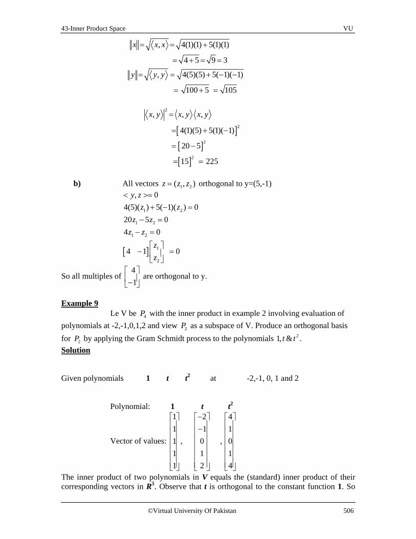
43-Inner Product Space VU
©Virtual University Of Pakistan 506
, 4(1)(1) 5(1)(1)
4 5 9 3
x x x= = +
= + = =
, 4(5)(5) 5( 1)( 1)
100 5 105
y y y= = + − −
= + =
[ ][ ][ ]
2
2
2
2
, , ,
4(1)(5) 5(1)( 1)
20 5
15 225
x y x y x y=
= + −
= −
= =
b) All vectors 1 2( , )z z z= orthogonal to y=(5,-1)
[ ]
1 2
1 2
1 2
1
2
, 04(5)( ) 5( 1)( ) 020 5 04 0
4 1 0
y zz z
z zz z
zz
< >=+ − =
− =− =
− =
So all multiples of 41
−
are orthogonal to y.
Example 9 Le V be 4P with the inner product in example 2 involving evaluation of polynomials at -2,-1,0,1,2 and view 2P as a subspace of V. Produce an orthogonal basis for 2P by applying the Gram Schmidt process to the polynomials 21, &t t . Solution Given polynomials 1 t t2 at -2,-1, 0, 1 and 2
Polynomial: 1 t t2
Vector of values:
1 2 41 1 1
, ,1 0 01 1 11 2 4
− −
The inner product of two polynomials in V equals the (standard) inner product of their corresponding vectors in R5. Observe that t is orthogonal to the constant function 1. So

43-Inner Product Space VU
©Virtual University Of Pakistan 507
take p0(t) = 1 and p1(t) = t. For p2, use the vectors in R5 to compute the projection of t2 onto Span {p0, p1}:
2 20
0 0
2 21
, ,1 4 1 0 1 4 10
, 5
, , 8 ( 1) 0 1 8 0
t p t
p p
t p t t
= = + + + + =
=
= = − + − + + + =
The orthogonal projection of t2 onto Span {1, t} is 0 110 0 .5
p p+ Thus 2 2
2 0( ) 2 ( ) 2p t t p t t= − = − An orthogonal basis for the subspace P2 of V is:
Polynomial: p0 p1 p2
Vector of values:
1 2 21 1 1
, ,1 0 21 1 11 2 2
− − − − −
Best Approximation in Inner Produce Spaces A common problem in applied mathematics involves a vector space V whose elements are functions. The problem is to approximate a function f in V by a function g from a specified subspace W of V. The “closeness” of the approximation of f depends on the way f g− is defined. We will consider only the case in which the distance between f and g is determined by an inner product. In this case the best approximation to f by functions in W is the orthogonal projection of f onto the subspace W. Example 10 Let V be 4P with the inner product in example 5 and let 0 1 2, &P P P be the orthogonal basis for the subspace 2P , find the best approximation to ( ) 415
2p t t= − by polynomials in 2P .
Solution: The values of p0, p1, and p2 at the numbers – 2, –1, 0, 1, and 2 are listed in R5 vectors in
Polynomial: p0 p1 p2

43-Inner Product Space VU
©Virtual University Of Pakistan 508
Vector of values:
1 2 21 1 1
, ,1 0 21 1 11 2 2
− − − − −
The corresponding values for p are: 3,9 2,5,9 2,− and –3. We compute
0 1 2
0 0 2 2
, 8 , 0 , 31
, 5, , 14
p p p p p p
p p p p
= = = −
= =
Then the best approximation in V to p by polynomials in P2 is
2
0 1 20 1 2
0 0 1 1 2 2
28 31 8 310 25 14 5 14
, , ,ˆ
, , ,
( 2).
p
p p p p p pp proj p p p p
p p p p p p
p p t−
= = + +
= + = − −
This polynomial is the closest to P of all polynomials in P2, when the distance between polynomials is measured only at –2, –1, 0, 1, and 2. Cauchy – Schwarz Inquality
,
,
For all u v in V
u v u v≤
Triangle Inequality
,For all u v in Vu v u v+ ≤ +
Proof
2 22 ,u u v v≤ + + 2 22u u v v≤ + +
( )22u v u v+ = +
u v u v⇒ + = +
Inner product for [ ],C a b
2 ,
, 2 , ,
u v u v u v
u u u v v v
+ = + +
= + +

43-Inner Product Space VU
©Virtual University Of Pakistan 509
Probably the most widely used inner product space for applications is the vector space [ ],C a b of all continuous functions on an interval a t b≤ ≤ , with an inner product that will describe. Example 11 For f , g in [ ],C a b , set
( ) ( ),a
bf g f t g t dt= ∫
Show that it defines an inner product on [ ],C a b . Solution
Inner product Axioms 1 to 3 follow from elementary properties of definite integrals
1. , ,
2. , , ,
3. , ,
f g g f
f h g f g h g
cf g c f g
=
+ = +
=
For Axiom 4, observe that 2, [ ( )] 0
b
af f f t dt= ≥∫
The function [f(t)]2 is continuous and nonnegative on [a, b]. If the definite integral of [f(t)]2 is zero, then [f(t)]2 must be identically zero on [a, b], by a theorem in advanced calculus, in which case f is the zero function. Thus ,f f = 0 implies that f is the zero function of [a, b].
So , ( ) ( )b
at t dt= ∫f g f g defines an inner product on C[a, b].
Example 12
Compute ,f g where [ ]2 3( ) 1 3 ( ) 0,1f t t and g t t t on v C= − = − = . Solution
Let V be the space [ ],C a b with the inner product
( ) ( ),a
bf g f t g t dt= ∫
2 3( ) 1 3 , ( )f t t g t t t= − = −
( )( )
1 2 3
01 5 3
01
6 4 2
0
, (1 3 )
3 4
1 12 2
0
f g t t t dt
t t t dt
t t t
= − −
= − +
= − +
=
∫∫
Example 13

43-Inner Product Space VU
©Virtual University Of Pakistan 510
Let V be the space [ ],C a b with the inner product
( ) ( ),a
bf g f t g t dt= ∫
Let W be the subspace spanned by the polynomials ( ) ( ) ( ) 2
1 2 31 , 2 1 & 12P t P t t P t t= = − = Use the Gram – Schmidt process to find an orthogonal basis for W. Solution Let q1 = p1, and compute
1
0
1 2
0, (2 1)(1) ( ) 0t dt t t= − = − =∫2 1p q
So p2 is already orthogonal to q1, and we can take q2 = p2. For the projection of p3 onto W2 = Span {q1, q2}, we compute
1
0
1 2 3
0, 12 1 4 4t dt t= ⋅ = =∫3 1p q
1
0
1
0, 1 1 1dt t= ⋅ = =∫1 1q q
1 12 3 2
0 0, 12 (2 1) (24 12 ) 2t t dt t t dt= − = − =∫ ∫3 2p q
1
0
1 2 3
0
1 1, (2 1) (2 1)6 3
t dt t= − = − =∫2 2q q
Then , , 4 2proj 4 6, , 1 1 3
= + = + = +2
3 1 3 2w 3 1 2 1 2 1 2
1 1 2 2
p q p qp q q q q q q
q q q q
And proj 4 6= − = − −23 3 w 3 3 1 2q p p p q q
As a function, q3(t) = 12t2 – 4 – 6(2t – 1) = 12t2 – 12t + 2. The orthogonal basis for the subspace W is {q1, q2, q3} Exercises
Let 2ℜ have the inner product of example 1 and let x=(1,1) and y=(5,-1) a) Find
2, ,x y and x y b) Describe all vectors ( )1 2,z z that are
orthogonal to y. 2) Let 2ℜ have the inner product of Example 1. Show that the Cauchy-Shwarz inequality holds for x=(3,-2) and y=(-2,1) Exercise 3-8 refer to 2P with the inner product given by evaluation at -1,0 and 1 in example 2. 3) Compute ,p q where p(t)= 4+t q(t) = 5-4t2
4) Compute ,p q where p(t)= 3t - t2 q(t) = 3 + t2
5) Compute P and q for p and q in exercise 3.
6) Compute P and q for p and q in exercise 4. 7) Compute the orthogonal projection of q onto the subspace spanned by p, for p and q in Exercise 3.

43-Inner Product Space VU
©Virtual University Of Pakistan 511
8) Compute the orthogonal projection of q onto the subspace spanned by p, for p and q in Exercise 4.
9) Let 3P have the inner product given by evaluation at -3,-1,1, and 3. Let
21 2( ) 1 , ( ) , ( )p t p t t and p t tο = = =
a)Computer the orthogonal projection of 2P on to the subspace spanned by 0P and 1P . b) Find a polynomial q that is orthogonal to 0P and 1P such tha { }0 1, ,p p q is an orthogonal
basis for span { }0 1, ,p p q . Scale the polynomial q so that its vector of values at (-3,-1,1,3) is (1,-1,-1,1)
10) Let 3P have the inner product given by evaluation at -3,-1,1, and 3. Let 2
1 2( ) 1 , ( ) , ( )p t p t t and p t tο = = = Find the best approximation to 3( )p t t= by polynomials in Span { }0 1, ,p p q .
11) Let 0 1 2, ,p p p be the orthogonal polynomials described in example 5, where the inner product on 4P is given by evaluation at -2, -1, 0, 1, and 2. Find the orthogonal projection of 3t onto Span { }0 1 2, ,p p p
12) Compute ,f g where [ ]2 3( ) 1 3 ( ) 0,1f t t and g t t t on v C= − = − = . 13) Compute ,f g where
[ ]3 2( ) 5 3 ( ) 0,1f t t and g t t t on v C= − = − = .
14) Compute f for f in exercise 12.
15) Compute g for g in exercise 13. 16) Let V be the space C[-2,2] with the inner product of Example 7. Find an
orthogonal basis for the subspace spanned by the polynomials 21, ,t t . 17)
Let 1
2
uu
u
=
and 1
2
vv
v
=
be two vectors in 2R . Show that 1 1 2 2, 2 3u v u v u v= +
defines an inner product.

44-Application of Inner Product Spaces VU
©Virtual University Of Pakistan 512
Lecture 44 Application of inner product spaces
Definition An inner product on a vector space V is a function that associates to each pair of vectors u and v in V, a real number ,u v and satisfies the following axioms, for all u, v, w in V and all scalars c: 1. , ,
2. , , ,
3. , ,
4. , 0 , 0 0.
u v v u
u v w u w v w
cu v c u v
u u and u u iff u
=
+ = +
=
≥ = =
A vector space with an inner product is called an inner product space. Least Squares Lines The simplest relation between two variables x and y is the linear equation 0 1y xβ β= + . Often experimental data produces points 1 1( , ),..., ( , )n nx y x y that when graphed, seem to lie close to a line. Actually we want to determine the parameters
0β and 1β that make the line as “close” to the points as possible. There are several ways to measure how close the line is to the data. The usual choice is to add the squares of the residuals. The least squares line is the line 0 1y xβ β= + that minimizes the sum of the squares of the residuals. If the data points are on the line, the parameters 0β and 1β would satisfy the equations
0 1 1 1
0 1 2 2
0 1
_________________
. .. .. .
n n
predicted Observedvalue value
x yx y
x y
β ββ β
β β
+ =+ =
+ =

44-Application of Inner Product Spaces VU
©Virtual University Of Pakistan 513
We can write this system as
01
2 1
0
1
11. . .
, ,. . .. . .1 n n
X yyx
x y
Where X y
x y
β
ββ
β
=
= = =
Computing the least-squares solution of X yβ = is equivalent to finding the β that determines the least-squares line. Example 1 Find the equation 0 1y xβ β= + of the least-squares line that best fits the data points (2, 1), (5, 2), (7, 3), (8, 3). Solution For the least-squares solution of x yβ = , obtain the normal equations(with the new notation) : ˆT TX X X yβ = i.e, compute
1 21 1 1 1 1 5 4 222 5 7 8 1 7 22 142
1 8
TX X
= =
11 1 1 1 2 92 5 7 8 3 57
3
TX y
= =
0
1
1 2 11 5 2
, ,1 7 31 8 3
X y
Here X y
β
ββ
β
=
= = =

44-Application of Inner Product Spaces VU
©Virtual University Of Pakistan 514
The normal equations are
0
1
4 22 922 142 57
ββ
=
Hence,
10
1
4 22 922 142 57
142 22 9122 4 5784
24 2 / 7130 5 /1484
ββ
−
=
− = −
= =
Thus, the least -squares line has the equation
2 57 14
y x= +
Weighted Least-Squares Let y be a vector of n observations, 1 2, ,..., ny y y and suppose we wish to approximate y by a vector y that belongs to some specified subspace of n
(as discussed previously that y is written as Ax so that y was in the column space of A).Now suppose the approximating vector y is to be constructed from the columns of matrix A. Then we find an x that makes ˆ ˆAx y= as close to y as possible. So that measure of closeness is the weighted error 2 2ˆ ˆWy Wy Wy WAy− = −

44-Application of Inner Product Spaces VU
©Virtual University Of Pakistan 515
Where W is the diagonal matrix with (positive) 1,..., nw w on its diagonal, that is
1
2
0 . . . 00. . .. . .. . .0 . . . n
ww
W
w
=
Thus, x is the ordinary least-squares solution of the equation WAx Wy= The normal equation for the weighted least-squares solution is ( ) ( )T TWA WAX WA Wy= Example 2 Find the least squares line 0 1y xβ β= + that best fits the data (–2, 3), (–1, 5), (0, 5), (1, 4), (2, 3). Suppose that the errors in measuring the y-values of the last two data points are greater than for the other points. Weight this data half as much as the rest of the data. Solution
0
1
,1 2 31 1 51 0 , , 51 1 41 2 3
Write X and y
X y
β
ββ
β
− − = = =
For a weighting matrix, choose W with diagonal entries 2 , 2 , 2 , 1 and 1. Left-multiplication by W scales the rows of X and y:
2 0 0 0 0 1 20 2 0 0 0 1 10 0 2 0 0 1 00 0 0 1 0 1 10 0 0 0 1 1 2
WX
− − =

44-Application of Inner Product Spaces VU
©Virtual University Of Pakistan 516
2 4 62 2 102 0 , 101 1 41 2 3
WX Wy
− − = =
For normal equation, compute
14 9 59( ) , ( )
9 25 34T TWX WX and WX Wy
− = = − −
And solve
0
1
10
1
0
1
0
1
0
1
14 9 599 25 34
14 9 599 25 34
25 9 5919 14 34269
25 9 5919 14 34269
1169 4.3155 0.2269
ββ
ββ
ββ
ββ
ββ
−
− = − −
− = − −
= −
= −
= =
Therefore, the solution to two significant digits is 0 14.3 0.20andβ β= = . Hence the required line is 4.3 0.2y x= + In contrast, the ordinary least-squares line for this data can be found as:
1 21 1
1 1 1 1 1 5 01 0
2 1 0 1 2 0 101 11 2
TX X
− − = = − −

44-Application of Inner Product Spaces VU
©Virtual University Of Pakistan 517
35
1 1 1 1 1 205
2 1 0 1 2 143
TX y
= = − − −
0
1
10
1
0
1
0
1
5 0 200 10 1
5 0 200 10 1
10 0 2010 5 150
200 4.015 0.150
ββ
ββ
ββ
ββ
−
= −
= −
= −
= = − −
Hence the equation of least-squares line is 1.0 0.1y x= −
What Does Trend Analysis Mean? An aspect of technical analysis that tries to predict the future movement of a stock based on past data. Trend analysis is based on the idea that what has happened in the past gives traders an idea of what will happen in the future.

44-Application of Inner Product Spaces VU
©Virtual University Of Pakistan 518
Linear Trend A first step in analyzing a time series, to determine whether a linear relationship provides a good approximation to the long-term movement of the series computed by the method of semi averages or by the method of least squares. Note The simplest and most common use of trend analysis occurs when the points 0 1, ,..., nt t t can be adjusted so that they are evenly spaced and sum to zero. Example Fit a quadratic trend function to the data (-2,3), (-1,5), (0,5), (1,4) and (2,3) Solution The t-coordinates are suitably scaled to use the orthogonal polynomials found in Example 5 of the last lecture. We have
0 1 2Polynomial : p p p data : g1 2 2 31 1 1 5
: 1 , 0 , 2 , 51 1 1 41 2 2 3
Vector of values
− − − − −
0 1 20 1 2
0 0 1 1 2 2
0 1 2
2
, , ,ˆ, , ,
20 1 75 10 14
ˆ ( ) 4 0.1 0.5( 2)
g p g p g pp p p pp p p p p p
p p p
and p t t t
< > < > < >= + +< > < > < >
= − −
= − − −
Since, the coefficient of 2p is not extremely small, it would be reasonable to conclude that the trend is at least quadratic.

44-Application of Inner Product Spaces VU
©Virtual University Of Pakistan 519
Above figure shows that approximation by a quadratic trend function Fourier series If f is a 2π -periodic function then
0
1( ) ( cos sin )
2 m mm
af t a mt b mt∞
=
= + +∑
is called Fourier series of f where
2
0
1 ( ) cosma f t mt dtπ
π= ∫ and
2
0
1 ( )sinmb f t mt dtπ
π= ∫
Example Let [0, 2 ]C π has the inner product
2
0
, ( ) ( )f g f t g t dtπ
< >= ∫
and let m and n be unequal positive integers. Show that cos mt and cos nt are orthogonal. Solution When m n≠
2
02
0
cos ,cos cos cos
1 [cos ( ) cos( )2
mt nt mt nt dt
mt nt mt nt dt
π
π
< >=
= + + −
∫
∫

44-Application of Inner Product Spaces VU
©Virtual University Of Pakistan 520
2
0
1 sin ( ) sin ( )2
0
mt nt mt ntm n m n
π+ − = + + −
=
Example Find the nth-order Fourier approximation to the function
( )f t t= on the interval[0,2 ]π . Solution We compute
2220
00
1 1 1 1.2 2 2 2a t dt t
ππ
ππ π
= = =
∫
and for k>0, using integration by parts,
22
200
22
200
1 1 1cos cos sin 0
1 1 1 2sin sin cos
k
k
ta t kt dt kt ktk k
tb t kt dt kt ktk k k
ππ
ππ
π π
π π
= = + =
= = − = −
∫
∫
Thus, the nth-order Fourier approximation of ( )f t t= is
2 22sin sin 2 sin 3 sin3
t t t ntn
π − − − − ⋅⋅⋅−
The norm of the difference between f and a Fourier approximation is called the mean square error in the approximation. It is common to write
0
1( ) ( cos sin )
2 m mm
af t a mt b mt∞
=
= + +∑
This expression for f (t) is called the Fourier series for f on[0,2 ]π . The term cosma mt , for example, is the projection of f onto the one-dimensional subspace spanned by cos mt .
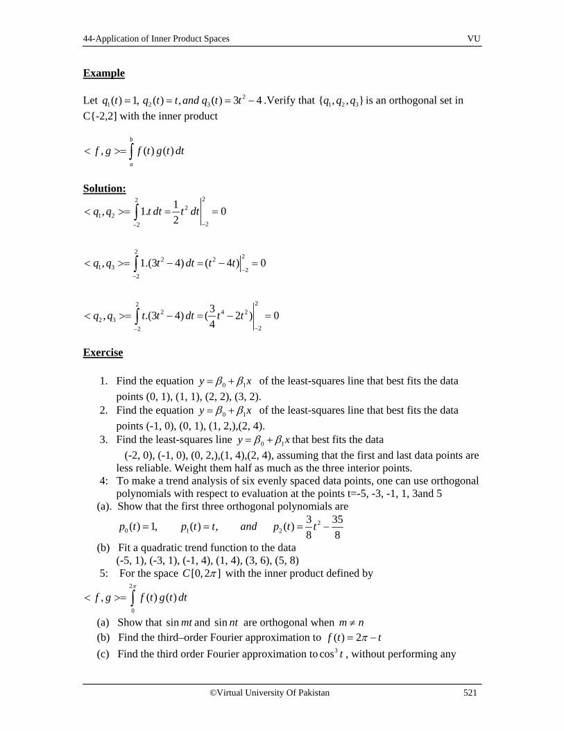
44-Application of Inner Product Spaces VU
©Virtual University Of Pakistan 521
Example Let 2
1 2 3( ) 1, ( ) , ( ) 3 4q t q t t and q t t= = = − .Verify that 1 2 3{ , , }q q q is an orthogonal set in C{-2,2] with the inner product
, ( ) ( )b
a
f g f t g t dt< >= ∫
Solution:
222
1 222
222 2
1 3 22
222 4 2
2 322
1, 1. 02
, 1.(3 4) ( 4 ) 0
3, .(3 4) ( 2 ) 04
q q t dt t dt
q q t dt t t
q q t t dt t t
−−
−−
−−
< >= = =
< >= − = − =
< >= − = − =
∫
∫
∫
Exercise
1. Find the equation 0 1y xβ β= + of the least-squares line that best fits the data points (0, 1), (1, 1), (2, 2), (3, 2).
2. Find the equation 0 1y xβ β= + of the least-squares line that best fits the data points (-1, 0), (0, 1), (1, 2,),(2, 4).
3. Find the least-squares line 0 1y xβ β= + that best fits the data (-2, 0), (-1, 0), (0, 2,),(1, 4),(2, 4), assuming that the first and last data points are less reliable. Weight them half as much as the three interior points.
4: To make a trend analysis of six evenly spaced data points, one can use orthogonal polynomials with respect to evaluation at the points t=-5, -3, -1, 1, 3and 5 (a). Show that the first three orthogonal polynomials are
20 1 2
3 35( ) 1, ( ) , ( )8 8
p t p t t and p t t= = = −
(b) Fit a quadratic trend function to the data (-5, 1), (-3, 1), (-1, 4), (1, 4), (3, 6), (5, 8) 5: For the space [0,2 ]C π with the inner product defined by
2
0
, ( ) ( )f g f t g t dtπ
< >= ∫
(a) Show that sin mt and sin nt are orthogonal when m n≠ (b) Find the third–order Fourier approximation to ( ) 2f t tπ= − (c) Find the third order Fourier approximation to 3cos t , without performing any

44-Application of Inner Product Spaces VU
©Virtual University Of Pakistan 522
integration calculations. 6: Find the first-order and third order Fourier approximations to
( ) 3 2sin 5sin 2 6cos 2f t t t t= − + −

45- Revision VU
©Virtual University Of Pakistan 523
Revision of Previous Lectures