Politecnico di Torino

Corso di Laurea Magistrale in Automotive Engineering

Tesi di Laurea Magistrale

VIRTUAL MODEL OF A VEHICLE ADAPTIVE DAMPER SYSTEM

Candidate Kyle Hugo

Relatore Prof. Nicola Amati

Torino, TO, Italia

©2019 Kyle Hugo

ii

Declaration of Originality

I hereby certify that I am the sole author of this thesis and that no part of this thesis has been

published or submitted for publication.

I certify that, to the best of my knowledge, my thesis does not infringe upon anyone’s copyright

nor violate any proprietary rights and that any ideas, techniques, quotations, or any other

material from the work of other people included in my thesis, published or otherwise, are fully

acknowledged in accordance with the standard referencing practices. Furthermore, to the

extent that I have included copyrighted material that surpasses the bounds of fair dealing

within the meaning of the Canada Copyright Act, I certify that I have obtained a written

permission from the copyright owner(s) to include such material(s) in my thesis and have

included copies of such copyright clearances to my appendix.

I declare that this is a true copy of my thesis, including any final revisions, as approved by my

thesis committee and the Graduate Studies office, and that this thesis has not been submitted

for a higher degree to any other University or Institution.

iii

Abstract

Several FCA vehicles are fitted with semi-active damper systems which modulate the level of damping

implemented in the vehicle suspension system to improve both the handling and ride quality felt by

vehicle’s occupants.

Durability simulations are necessary to analyze a vehicle’s or a component’s structural integrity over an

expected lifespan. Performing durability simulations in a virtual environment has streamlined the

traditional development cycle by reducing the need to construct physical prototypes and conduct

physical road or bench tests. It is essential that the vehicle is modeled as accurately as possible in the

virtual environment to ensure the results are representative of real-world performance.

Presently, the incorporation of a semi-active damper system in a virtual durability simulation involves

the expensive and resource intensive use of empirically obtained data. The goal of this project is to

improve the fidelity and efficiency of durability simulations by including the loading effects of a semi-

active suspension system. To accomplish this, several semi active suspension control algorithms and

practical considerations are studied. Using a car model developed in Simulink©, a neural network,

clipped optimal control, and sliding mode control algorithms are developed to approximate operating

characteristics of the supplier controller. The development of each controller, along with appropriate

tuning and validation procedures in Simulink©, are presented.

A process known as co-simulation is then used to integrate each of the chosen semi-active damper

control systems into durability simulations used in vehicle development processes at FCA. Co-simulation

is a process wherein the controller is executed in parallel with MSC Adams© CAE durability simulation

software using Matlab©/Simulink©. The accuracy of the neural network, sliding mode controller, and

clipped optimal controller are validated by correlating results to a Co-simulation carried out with a

supplier controller.

It is found that the performance of the neural network controller resulted in output chattering

throughout the simulation. While performance is acceptable in ranges where the output data is

expected to be low frequency and low amplitude, instances where this was not the case induced

chattering events. These events are most likely due to the neural network receiving inputs outside of the

range of data which it was trained on.

iv

Dedication

I would like to take a hot minute to thank all the CAE simulation staff at FCA that put up with my

incessant questions and disasters, including; Chandra Tangella, Khanh Nguyen, Daniel Liang and Ali

Jahroumi. I would also like to thank Marie Mills of ARDC and Dr. Jennifer Johrendt of the University of

Windsor for always trying their hardest to keep this program running smoothly.

However, this thesis is dedicated to Reza Atashrazm, without whose help and unfailing patience, I would

still be trying to open a .adm file in Motionview.

v

Contents

Declaration of Originality .............................................................................................................................. ii

Abstract ........................................................................................................................................................ iii

Dedication .................................................................................................................................................... iv

List of Figures ............................................................................................................................................. viii

List of Tables ............................................................................................................................................... xii

List of Variables ...........................................................................................................................................xiii

List of Abbreviations ................................................................................................................................... xiv

Note on Confidentiality ............................................................................................................................... xiv

1. Introduction .......................................................................................................................................... 1

1.1. Background ................................................................................................................................... 1

1.1.1. Active and Semi-Active Suspension Systems ........................................................................ 1

1.1.2. Vehicle Durability Testing ..................................................................................................... 3

1.1.3. Current Simulation Strategy .................................................................................................. 4

1.2. Project Motivation ........................................................................................................................ 7

1.3. Organization of the Thesis ............................................................................................................ 8

2. Literature Review .................................................................................................................................. 9

2.1. Skyhook Control ............................................................................................................................ 9

2.2. Clipped Optimal Control ............................................................................................................. 10

2.2.1. Quarter Car ......................................................................................................................... 10

2.2.2. Full Car Ride Model ............................................................................................................. 13

2.2.3. Physical Test Vehicle Experimental Results ........................................................................ 15

2.3. Neural Network General Background ......................................................................................... 15

2.4. Neural Network Application to Dampers in Durability Simulations ........................................... 19

2.5. Sliding Mode Control .................................................................................................................. 20

2.5.1. Controller Construction ...................................................................................................... 20

2.5.2. Simulation Results ............................................................................................................... 23

3. Controller Development ..................................................................................................................... 23

3.1. Clipped Optimal Controller Development .................................................................................. 24

3.1.1. Matlab© Quarter Car .......................................................................................................... 24

vi

3.1.2. Matlab© Full Car ................................................................................................................. 28

3.1.3. Full Car Controller Simulation Results ................................................................................ 31

3.2. Neural Network Controller Implementation .............................................................................. 34

3.2.1. Data acquisition .................................................................................................................. 34

3.2.2. Varying Road Profile Architecture Sensitivity ..................................................................... 35

3.2.3. Rough Road Input Network Construction Modifications and Hysteresis Data ................... 39

3.2.4. Durability Road Transfer Function Network Construction ................................................. 42

3.3. Sliding Mode Controller Development ....................................................................................... 47

3.3.1. Preliminary Development ................................................................................................... 47

3.3.2. Matlab©/Simulink© Full Car .............................................................................................. 52

3.3.3. Results ................................................................................................................................. 58

4. Durability Simulation Full Vehicle Model - Adams© .......................................................................... 62

4.1. Adams©/Controls State Variable Setup ..................................................................................... 63

4.1.1. Plant inputs setup – Forces ................................................................................................. 63

4.1.2. Outputs setup – Damper velocity, body acceleration, etc. ................................................ 64

4.2. Damper Element Replacement ................................................................................................... 65

4.3. Adams© Simulation Setup .......................................................................................................... 66

4.3.1. Setup Controls Plant ........................................................................................................... 68

4.4. Matlab© / Simulink© Setup ....................................................................................................... 68

4.4.1. Matlab© Initialization ......................................................................................................... 69

4.4.2. Simulink© Setup ................................................................................................................. 69

4.5. Co-simulation Validation ............................................................................................................. 73

5. Controller Co-simulation Implementation .......................................................................................... 76

5.1. Simulation Setup ......................................................................................................................... 76

5.2. Supplier Controller ...................................................................................................................... 76

5.2.1. Model Adjustments ............................................................................................................. 76

5.2.2. Simulink© Setup ................................................................................................................. 77

5.3. Neural Network Controller ......................................................................................................... 78

6. Co-simulation Results ......................................................................................................................... 80

6.1. Results – Neural Network Controller .......................................................................................... 80

6.1.1 Time History Force Output .................................................................................................. 80

6.1.2 Durability Calculations ........................................................................................................ 86

6.2. Analysis - Neural Network Controller Co-simulation. ................................................................. 89

vii

6.2.1. Time History Analysis .......................................................................................................... 89

6.2.2. Durability Analysis ................................................................................................................... 90

7. Conclusions and Recommendations ................................................................................................... 92

7.1. Conclusions ................................................................................................................................. 92

7.1.1. Clipped Optimal Controller ................................................................................................. 92

7.1.2. Neural Network Controller ................................................................................................. 92

7.1.3. Sliding Mode Controller ...................................................................................................... 93

7.1.4. Durability Simulation Implementation ............................................................................... 93

7.1.5. Overall ................................................................................................................................. 94

7.2. Recommendations ...................................................................................................................... 94

7.2.1. Neural Network Controller ................................................................................................. 94

7.2.2. Sliding Mode Controller ...................................................................................................... 95

7.2.3. Overall ................................................................................................................................. 95

References .................................................................................................................................................. 97

Appendix A – Simulink© Full Vehicle Ride Model ...................................................................................... 99

Overview ................................................................................................................................................. 99

Model Inputs & Outputs ......................................................................................................................... 99

Equations of Motion ............................................................................................................................. 100

Simulink© Block Architecture ............................................................................................................... 101

Parameters ............................................................................................................................................ 104

Assumptions, Simplifications and Potential Improvements ................................................................. 105

viii

List of Figures

Figure 1: The damping stiffness of a vehicle is chosen based on its intended use....................................... 1

Figure 2: Active suspension quarter car model with force actuator in parallel with spring and damper

elements [1] .................................................................................................................................................. 2

Figure 3: Semi-Active suspension quarter car model with adjustable damper [1] ...................................... 2

Figure 4: Discrete semi-active damper curves (Jounce negative) ................................................................ 5

Figure 5: Damper curve selection algorithm for hybrid durability simulations ............................................ 6

Figure 6: Comparison of durability simulation damper force methods: Direct (red), Using voltage output

in conjunction with damper curves (blue) .................................................................................................... 7

Figure 7: Skyhook model ............................................................................................................................... 9

Figure 8: Quarter car model used for controller development in [8] and [9]. ........................................... 11

Figure 9: 2-5-1 MLP Neural network [2] ..................................................................................................... 16

Figure 10: schematic of ith perceptron and activation function [2] ............................................................ 16

Figure 11: Sigmoid tangent activation function [10]. ................................................................................. 17

Figure 12: General network schematic for gradient descent training method explanation [2] ................. 18

Figure 13: Histogram of network weights used to evaluate network quality [2]. ...................................... 19

Figure 14: Reference Skyhook damping model [12] ................................................................................... 21

Figure 15: Simulink© Optimal controller and quarter car model diagram ................................................ 25

Figure 16: Time domain plot of vertical sprung body acceleration of quarter car models with clipped

optimal controlled and passive damping .................................................................................................... 26

Figure 17: Time domain plot of damper force of quarter car models with clipped optimal controlled and

passive damping .......................................................................................................................................... 27

Figure 18: Vertical sprung mass body acceleration estimated amplitude spectrum of Clipped optimal

controlled damping and passive damping .................................................................................................. 28

Figure 19: Full car Simulink© model with clipped optimal controller ........................................................ 29

Figure 20: Clipped optimal control damper output curve selection Simulink© Model ............................. 30

Figure 21: Front left damper force time history curve of Pattern Search optimized clipped optimal

controller and supplier controller ............................................................................................................... 31

Figure 22: Front left damper force time history curve of particle swarm optimized clipped optimal

controller and supplier controller ............................................................................................................... 32

ix

Figure 23: Rear left damper force time history curve of particle swarm optimized clipped optimal

controller and supplier controller ............................................................................................................... 33

Figure 24: Training road input dataset ....................................................................................................... 35

Figure 25: Matlab© GUI for creating neural networks ............................................................................... 36

Figure 26: Baseline neural network architecture, a visual representation ................................................ 36

Figure 27: 11-20-4 network test: ISO 2681 D-Class road profile ................................................................ 38

Figure 28: 11-20-4 network test: ISO 2681 B-Class road profile ................................................................. 38

Figure 29: 11-20-4 network test: Step Input ............................................................................................... 39

Figure 30: Road profile used to create more relevant training data .......................................................... 40

Figure 31: Best performing neural network for rough road - HPcSns1_ruf_FL .......................................... 42

Figure 32: Durability road amplitude spectrum (OG) and replicating transfer function (TF) ..................... 43

Figure 33: Durability road PSD (OG) and replicating transfer function (TF) ............................................... 44

Figure 34: Training, Validation, and Test Data similar to the durability road profile ................................. 45

Figure 35: Best performing neural network the durability road transfer function - PcSns3_RT_FL .......... 47

Figure 36: Simulink© SMC model diagram ................................................................................................. 48

Figure 37: Time history of vertical body acceleration and damper force for SMC and passive systems ... 50

Figure 38: Sprung body mass vertical acceleration amplitude spectrum ................................................... 51

Figure 39: Damper force amplitude spectrum............................................................................................ 51

Figure 40: Full car Simulink© model with individual corner SMC block ..................................................... 53

Figure 41: Half car SMC controller reference model .................................................................................. 54

Figure 42: Full car Simulink© model controlled by two half car based sliding mode controllers .............. 57

Figure 43: Time history results of individual wheel sliding mode control tuned with pattern search

optimization ................................................................................................................................................ 59

Figure 44: Time history results of half car model based Sliding Mode control tuned with Pattern Search

Optimization ............................................................................................................................................... 61

Figure 45: Adams© State Variable setup window for damper force plant input ....................................... 64

Figure 46: Adams© State Variable setup window for plant outputs ......................................................... 64

Figure 47: Adams© direct single component force element specification window - Front ...................... 65

Figure 48: Adams© direct single component force element specification window - Rear ........................ 65

Figure 49: Original passive damper element .............................................................................................. 66

Figure 50: ADS co-simulation damper direct single component force (damper suppressed temporarily for

visualization purposes) ............................................................................................................................... 66

x

Figure 51: Full vehicle analysis file driven event setup window ................................................................. 67

Figure 52: Adams©/Controls Plant Export window ................................................................................... 68

Figure 53: Matlab© workspace generated by executing the .m file from the plant export utility ............ 69

Figure 54: Matlab© command window Adams© plant actuators (inputs to Adams©) and sensors

(outputs from Adams©) after running .m file from the plant export utility .............................................. 69

Figure 55: .m file required modifications for Linux..................................................................................... 69

Figure 56: Generated Adams_sys.slx file containing Simulink© blocks linking to Adams© model ........... 70

Figure 57: Passively damped Adams© Co-simulation Simulink© model ................................................... 71

Figure 58: Co-simulation configuration parameters setup window ........................................................... 72

Figure 59: Block diagram within adams_sub block ..................................................................................... 73

Figure 60: adams_plant block parameters ................................................................................................. 73

Figure 61: Damper velocity plot of passive system executed purely in Adams© (red) and using Co-

simulation, measured with built in damper output (blue) and measured with output state variable (pink)

.................................................................................................................................................................... 74

Figure 62: Damper force plot of passive system executed purely in Adams© (red) and using Co-

simulation (blue). The overlap of the two outputs indicates that the points in which velocity is measured

from does not hinder damper force implementation ................................................................................ 74

Figure 63: Supplier controller co-simulation acceleration output marker declaration .............................. 77

Figure 64: Supplier controller co-simulation body acceleration plant output state variable declaration . 77

Figure 65: Supplier controller co-simulation vertical body - wheel relative displacement plant output

state variable declaration ........................................................................................................................... 77

Figure 66: Simulink© block diagram for Adams© co-simulation with supplier controller ........................ 78

Figure 67: Simulink© block diagram for Adams© co-simulation with neural network controllers ........... 79

Figure 68: Linear regression plots between neural network controlled and supplier controlled dampers

at each vehicle corner. ................................................................................................................................ 81

Figure 69: Front left damper force time history output - Neural network controller and supplier

controller..................................................................................................................................................... 82

Figure 70: Front right damper force time history output - Neural network controller and supplier

controller..................................................................................................................................................... 83

Figure 71: Rear left damper force time history output - Neural network controller and supplier controller

.................................................................................................................................................................... 84

xi

Figure 72: Rear Right damper force time history output - Neural network controller and supplier

controller..................................................................................................................................................... 85

Figure 73: Overall Max/Min loads output by dampers comparison ........................................................... 87

Figure 74: Damage ratio - Neural network controller versus Supplier controller ...................................... 88

Figure 75: Simulink© full car ride model schematic ................................................................................... 99

Figure 76: Wheel Equation of motion (46) Simulink© Model .................................................................. 102

Figure 77: Vehicle body Equations of motion (48), (49), & (50) Simulink© model .................................. 103

Figure 78: Centroid accelerations to corner displacement conversion Simulink© block ........................ 103

Figure 79: Simulink© full car ride model .................................................................................................. 104

xii

List of Tables

Table 1: SMC gain example values [12] ...................................................................................................... 22

Table 2: Clipped optimal controller tuning weights ................................................................................... 26

Table 3: Error results of clipped optimal controller with pattern search optimized weights .................... 31

Table 4: Error results of clipped optimal controller with particle swarm optimized weights .................... 33

Table 5: Neural Network input and output data channels ......................................................................... 34

Table 6: Initial neural network training parameters ................................................................................... 36

Table 7: Initial neural network perceptron sensitivity ................................................................................ 37

Table 8: Initial neural network layer sensitivity .......................................................................................... 37

Table 9: FL Damper Neural network layer size sensitivity for rough road input ........................................ 41

Table 10: FL Damper Neural network layer size sensitivity for rough road input with History .................. 41

Table 11: FL Damper Neural network layer size sensitivity for the durability road transfer function input

.................................................................................................................................................................... 46

Table 12: FL Damper Neural network layer size sensitivity for the durability road transfer function input

with history inputs ...................................................................................................................................... 46

Table 13: Quarter car simulation parameter values [12] ........................................................................... 49

Table 14: Optimized quarter car model-based SMC tuning parameters .................................................... 58

Table 15: Error results of quarter car model based Sliding Mode Control tuned with Pattern Search

Optimization ............................................................................................................................................... 59

Table 16: Half car model based sliding mode controller optimized controller tuning parameters ........... 60

Table 17: Error results of half car model based Sliding Mode Control tuned with Pattern Search

Optimization ............................................................................................................................................... 61

Table 18: Semi-active damper force linear regression – Neural network controller ................................. 80

Table 19: Overall Max/Min loads output by dampers - Supplier controller ............................................... 87

Table 20: Overall Max/Min loads output by dampers - Neural Network controller .................................. 87

Table 21: Calculated damage for 100 cycles - Neural network controller .................................................. 88

Table 22: Calculated damage for 100 cycles - Supplier controller .............................................................. 88

xiii

List of Variables

𝐴 State space state matrix

𝐵 State space input to state matrix

𝑏𝑖 Neural network bias for perceptron i

𝐶 State space to output matrix

𝐶𝑑𝑝 Passive damping

𝐶𝑆𝑘𝑦 Skyhook damping coefficient

𝐶𝑡 Tire damping

𝐷 State space feed through matrix

𝑒 Sliding mode control actual – ideal system error

𝑓𝑑0 Sliding mode control base desirable damping force

𝐹𝑠 Damper force state space input vector

𝐹𝑆𝐷 Corner spring + damper force

𝐹𝑆𝑘𝑦 Skyhook damping force

𝐼𝜙 Sprung body pitch inertia

𝐼𝜃 Sprung body roll inertia

𝐽 Optimal control cost function

𝐾 Sliding mode control gain

𝑘𝑠 Spring stiffness

𝑘𝑡 Tire stiffness

𝑀𝑏 Sprung body mass

𝑀𝑤 Unsprung wheel mass

𝑁 Complete state vector to damper velocity conversion

𝑄 Optimal control state weight matrix

𝑅 Optimal control input weight matrix

𝑆 Sliding mode control sliding surface

𝑢 Controlled corner damper force

𝑤𝑖,𝑗 Neural network weight for perceptron i and input j

𝑋 State space state vector

𝑥𝑖 Neural network input

𝑦𝑖 Neural network output

𝑧𝑏 Sprung body mass vertical displacement

𝑧𝑟 Road input vertical displacement

𝑧𝑤 Unsprung wheel mass vertical displacement

𝛼 Neural network momentum

𝜂 Neural network learning rate

𝜃𝑏 Sprung body mass roll displacement

𝜙𝑏 Sprung body mass pitch displacement

𝜇 Neural network early stopping parameter

xiv

List of Abbreviations

1. FCA – Fiat Chrysler Automobiles

2. LQR – Linear Quadratic Regulator

3. SMC – Sliding Mode Control

4. ADS – Adaptive Damper System

5. FLC – Fuzzy Logic Controller

6. PSV – Passive

7. PSD – Power Spectral Density

8. GUI – Graphic User Interface

9. NN – Neural Network

10. FL – Front Left

11. FR – Front Right

12. RL – Rear Left

13. RR – Rear Right

Note on Confidentiality

Due to confidentiality concerns concerning the contents of this work in regards to Fiat Chrysler

Automobiles, some figures, plots, and tables have had their information removed or normalized.

1. Introduction

To remain competitive in today’s global vehicle market, several FCA vehicle offerings are fitted with

advanced suspension systems. These systems have the capability of modifying suspension parameters to

improve comfort or handling based on a given road condition and driver preferences.

1.1. Background

1.1.1. Active and Semi-Active Suspension Systems

Comfort and handling are two conflicting performance objectives faced in the design of any vehicle’s

suspension system [1]. A damping setting with a higher damping coefficient can improve handling by

quickly dissipating oscillations. Conversely, a softer damping setting that dissipates less energy via a

lower damping coefficient reduces the magnitude of accelerations felt by the occupants in the sprung

vehicle body, thus improving perceived comfort. In a passive suspension system this introduces a

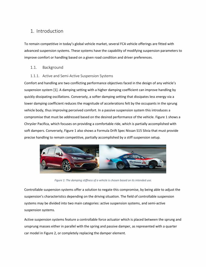
compromise that must be addressed based on the desired performance of the vehicle. Figure 1 shows a

Chrysler Pacifica, which focuses on providing a comfortable ride, which is partially accomplished with

soft dampers. Conversely, Figure 1 also shows a Formula Drift Spec Nissan S15 Silvia that must provide

precise handling to remain competitive, partially accomplished by a stiff suspension setup.

Figure 1: The damping stiffness of a vehicle is chosen based on its intended use.

Controllable suspension systems offer a solution to negate this compromise, by being able to adjust the

suspension’s characteristics depending on the driving situation. The field of controllable suspension

systems may be divided into two main categories: active suspension systems, and semi-active

suspension systems.

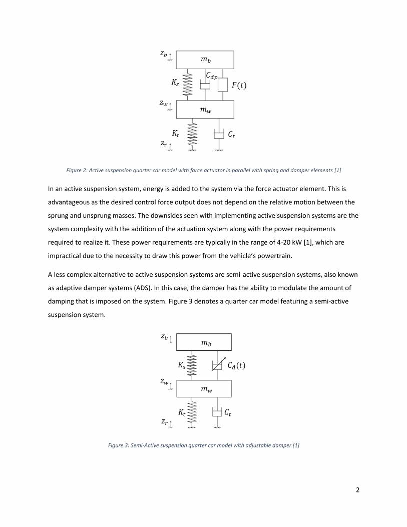
Active suspension systems feature a controllable force actuator which is placed between the sprung and

unsprung masses either in parallel with the spring and passive damper, as represented with a quarter

car model in Figure 2, or completely replacing the damper element.

2

Figure 2: Active suspension quarter car model with force actuator in parallel with spring and damper elements [1]

In an active suspension system, energy is added to the system via the force actuator element. This is

advantageous as the desired control force output does not depend on the relative motion between the

sprung and unsprung masses. The downsides seen with implementing active suspension systems are the

system complexity with the addition of the actuation system along with the power requirements

required to realize it. These power requirements are typically in the range of 4-20 kW [1], which are

impractical due to the necessity to draw this power from the vehicle’s powertrain.

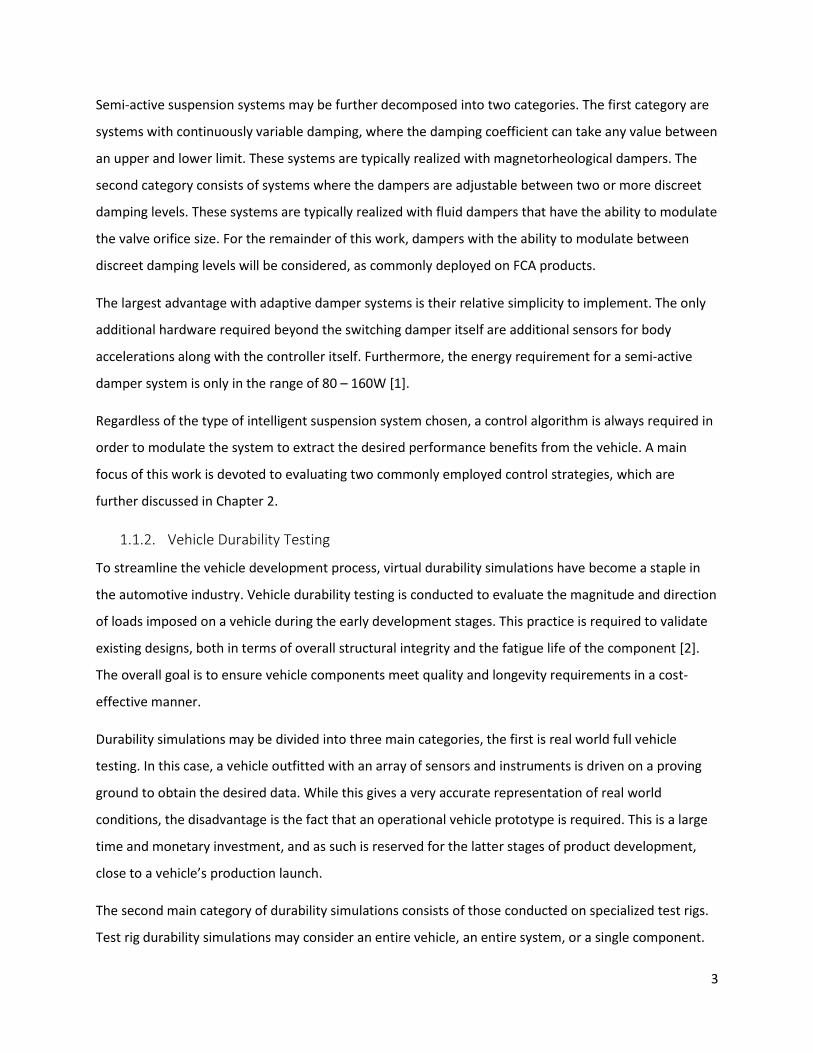
A less complex alternative to active suspension systems are semi-active suspension systems, also known

as adaptive damper systems (ADS). In this case, the damper has the ability to modulate the amount of

damping that is imposed on the system. Figure 3 denotes a quarter car model featuring a semi-active

suspension system.

Figure 3: Semi-Active suspension quarter car model with adjustable damper [1]

3

Semi-active suspension systems may be further decomposed into two categories. The first category are

systems with continuously variable damping, where the damping coefficient can take any value between

an upper and lower limit. These systems are typically realized with magnetorheological dampers. The

second category consists of systems where the dampers are adjustable between two or more discreet

damping levels. These systems are typically realized with fluid dampers that have the ability to modulate

the valve orifice size. For the remainder of this work, dampers with the ability to modulate between

discreet damping levels will be considered, as commonly deployed on FCA products.

The largest advantage with adaptive damper systems is their relative simplicity to implement. The only

additional hardware required beyond the switching damper itself are additional sensors for body

accelerations along with the controller itself. Furthermore, the energy requirement for a semi-active

damper system is only in the range of 80 – 160W [1].

Regardless of the type of intelligent suspension system chosen, a control algorithm is always required in

order to modulate the system to extract the desired performance benefits from the vehicle. A main

focus of this work is devoted to evaluating two commonly employed control strategies, which are

further discussed in Chapter 2.

1.1.2. Vehicle Durability Testing

To streamline the vehicle development process, virtual durability simulations have become a staple in

the automotive industry. Vehicle durability testing is conducted to evaluate the magnitude and direction

of loads imposed on a vehicle during the early development stages. This practice is required to validate

existing designs, both in terms of overall structural integrity and the fatigue life of the component [2].

The overall goal is to ensure vehicle components meet quality and longevity requirements in a cost-

effective manner.

Durability simulations may be divided into three main categories, the first is real world full vehicle

testing. In this case, a vehicle outfitted with an array of sensors and instruments is driven on a proving

ground to obtain the desired data. While this gives a very accurate representation of real world

conditions, the disadvantage is the fact that an operational vehicle prototype is required. This is a large

time and monetary investment, and as such is reserved for the latter stages of product development,

close to a vehicle’s production launch.

The second main category of durability simulations consists of those conducted on specialized test rigs.

Test rig durability simulations may consider an entire vehicle, an entire system, or a single component.

4

The key advantage to test rig simulations is the controlled environment in which they are performed,

aiding in improving the repeatability of results. However, much like full car simulations, a drawback is

that a physical vehicle or component is required to conduct the experiment.

The previous two methods of durability testing both have the drawback that a physical vehicle or

component is requirement before the simulation may be performed. Usually, these physical examples

are only available in the later stages of product development, where product changes are costly to

effect. The third category of durability simulations takes place in a virtual environment, eliminating the

requirement for a physical prototype. An additional advantage to virtual durability testing is the speed

at which cyclic process of testing, analysis, modification, and retesting may be executed. Moreover, the

fact that this process may be executed in the early phases of the design cycle results in expense

reductions. This is because changes can be made, and designs may be optimized before resources are

invested into the construction of physical prototypes.

A disadvantage of virtual durability simulations is the necessity that the virtual model must be

representative of the physical component or vehicle. Modelling complex machinery assemblies, like

automobiles, requires simplifications and assumptions. In the case of durability simulations, steps must

be taken to reduce these assumptions and increase the fidelity of the models used. Examples include

more accurate bushings models [2], including flexible bodies, and in the case of this work, integrating

the effects of semi-active suspension systems. Doing so helps to ensure that results from simulation will

accurately reflect what will be seen when physical prototypes are tested on finalized designs.

1.1.3. Current Simulation Strategy

Semi-active suspension systems currently installed on FCA products are of the discrete modulation type

described in Section 1.1.1. In this case, each damper has a hard and soft setting for both rebound and

jounce travel. This implies that the damper may be in one of four possible settings, and therefore be

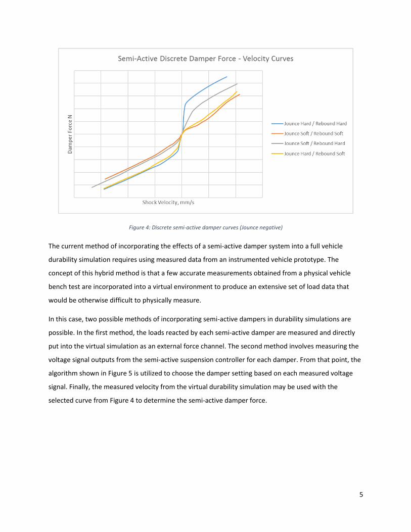
operating on one of four damper curves as shown in Figure 4.

5

Figure 4: Discrete semi-active damper curves (Jounce negative)

The current method of incorporating the effects of a semi-active damper system into a full vehicle

durability simulation requires using measured data from an instrumented vehicle prototype. The

concept of this hybrid method is that a few accurate measurements obtained from a physical vehicle

bench test are incorporated into a virtual environment to produce an extensive set of load data that

would be otherwise difficult to physically measure.

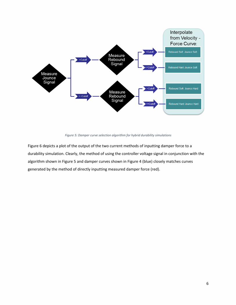
In this case, two possible methods of incorporating semi-active dampers in durability simulations are

possible. In the first method, the loads reacted by each semi-active damper are measured and directly

put into the virtual simulation as an external force channel. The second method involves measuring the

voltage signal outputs from the semi-active suspension controller for each damper. From that point, the

algorithm shown in Figure 5 is utilized to choose the damper setting based on each measured voltage

signal. Finally, the measured velocity from the virtual durability simulation may be used with the

selected curve from Figure 4 to determine the semi-active damper force.

6

Figure 5: Damper curve selection algorithm for hybrid durability simulations

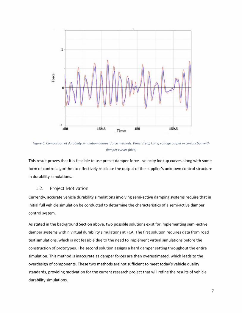
Figure 6 depicts a plot of the output of the two current methods of inputting damper force to a

durability simulation. Clearly, the method of using the controller voltage signal in conjunction with the

algorithm shown in Figure 5 and damper curves shown in Figure 4 (blue) closely matches curves

generated by the method of directly inputting measured damper force (red).

7

Figure 6: Comparison of durability simulation damper force methods: Direct (red), Using voltage output in conjunction with

damper curves (blue)

This result proves that it is feasible to use preset damper force - velocity lookup curves along with some

form of control algorithm to effectively replicate the output of the supplier’s unknown control structure

in durability simulations.

1.2. Project Motivation

Currently, accurate vehicle durability simulations involving semi-active damping systems require that in

initial full vehicle simulation be conducted to determine the characteristics of a semi-active damper

control system.

As stated in the background Section above, two possible solutions exist for implementing semi-active

damper systems within virtual durability simulations at FCA. The first solution requires data from road

test simulations, which is not feasible due to the need to implement virtual simulations before the

construction of prototypes. The second solution assigns a hard damper setting throughout the entire

simulation. This method is inaccurate as damper forces are then overestimated, which leads to the

overdesign of components. These two methods are not sufficient to meet today’s vehicle quality

standards, providing motivation for the current research project that will refine the results of vehicle

durability simulations.

8

To date, there have been several logical reasons why the effects of a semi-active damper system have

not been incorporated into virtual durability simulations. The first, and most prevalent, is that the

controller structure is proprietary to the original supplier of the semi-active damper system. As such it is

not available in detail to be examined by FCA. As such, it is required that this work develop its own

control algorithm capable of replicating both this supplier’s controller as well as any implemented going

forward.

Another key reason as to why a respective controller algorithm has not been acquired by FCA, is that

instances where it has been critical to understand semi-active damper controller effects on vehicle

performance often only consider a singular event. Examples include hard acceleration, heavy braking, a

moose test, etc. In these events, it is far easier to track the state of the damper throughout due to the

short time duration. This situation differs from a full durability simulation which consists of a complete

road profile composed of many events over a long period of time.

1.3. Organization of the Thesis

Chapter 2 of this work contains a literature review containing the semi-active suspension control

techniques chosen in this work. These control techniques include clipped optimal control, neural

networks, and sliding mode control. The mathematical background of each of these control strategies is

explored, and performance results from literature sources are displayed.

Moving forward, Chapter 3 focuses on Simulink© controller modelling. The performance of clipped

optimal and sliding mode controllers are examined using a quarter car model. A Simulink© full car ride

model is developed and used to examine controller performance and to efficiently tune controller

parameters using optimization techniques. This same full car ride model is used to generate data in

order to create neural network controllers. Finally, final controller structures are chosen for co-

simulation.

Chapters 4 and 5 bring the union of the control structures developed in Simulink© to virtual durability

simulations in MSC Adams©. First, in Chapter 4, an Adams© model is modified to integrate semi-active

suspension with co-simulation. Methodology for how control structures chosen in Chapter 3 are

integrated into durability simulations using co-simulation is discussed in Chapter 5.

Chapter 6 presents the results for how well the selected control algorithms perform in conjunction with

the full car durability model when compared to a supplier controller. Chapter 7 goes on to include a

discussion about the results of each set, as well as recommendations for future work.

9

2. Literature Review

2.1. Skyhook Control

It is impossible to discuss semi active damping systems without mentioning the concept of Skyhook

damping. Skyhook control was one of the first control models developed for an adaptive damping

system in the 1970s by Karnopp et al. [3] and remains a commonly referenced model in the realm of

adaptive suspension design.

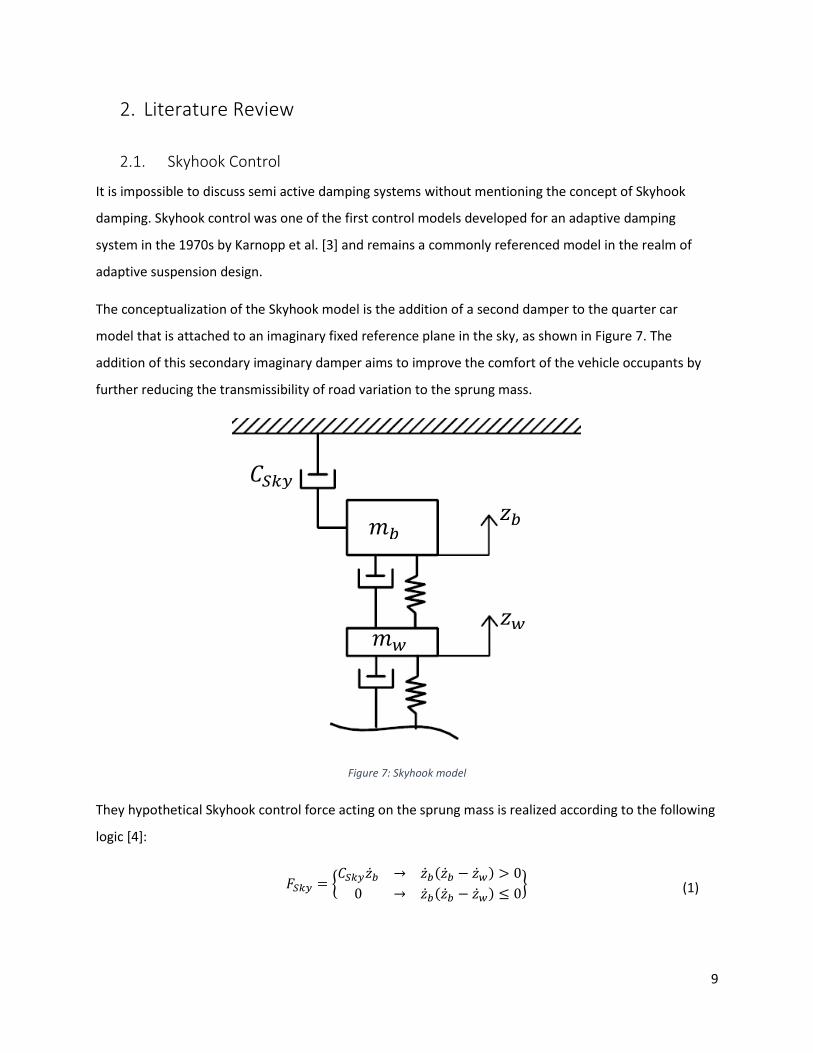
The conceptualization of the Skyhook model is the addition of a second damper to the quarter car

model that is attached to an imaginary fixed reference plane in the sky, as shown in Figure 7. The

addition of this secondary imaginary damper aims to improve the comfort of the vehicle occupants by

further reducing the transmissibility of road variation to the sprung mass.

Figure 7: Skyhook model

They hypothetical Skyhook control force acting on the sprung mass is realized according to the following

logic [4]:

𝐹𝑆𝑘𝑦 = {𝐶𝑆𝑘𝑦�̇�𝑏 → �̇�𝑏(�̇�𝑏 − �̇�𝑤) > 0

0 → �̇�𝑏(�̇�𝑏 − �̇�𝑤) ≤ 0} (1)

𝑚𝑏

𝑚𝑤

𝑧𝑏

𝑧𝑤

𝐶𝑆𝑘𝑦

10

It was determined via Simulink© simulation in [4] that the implementation of a simple Skyhook damper

controller dramatically reduced the transmissibility of a step road input to the vehicle unsprung mass,

and therefore the occupants.

Obviously, the idea of Skyhook control is impossible to implement on a real vehicle, but is considered as

a conceptual ideal system. Several methods have been deployed to practically implement this concept

however, using methods such as direct implementation [5], fuzzy logic [6] [7], and sliding mode control.

The latter is discussed in Section 2.5.

2.2. Clipped Optimal Control

[8] Focuses on the design and implementation of an optimal control scheme that goes beyond the

traditional input of only measured vehicle states. In this case, driver inputs such as braking, acceleration,

and cornering, in the form of inertial loads are considered mathematically as inertial forces acting on the

vehicle body. The purpose of this method is to create a more complete control structure, as the

controller can accommodate the additional large force variation on the suspension system implemented

by handling inputs.

2.2.1. Quarter Car

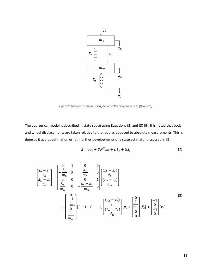
A modification is made to the quarter car model in [9] as can be seen in the Figure 8. The system

includes three inputs: damping coefficient, where: 𝑐𝑚𝑖𝑛 ∗ (�̇�𝑏 − �̇�𝑤) ≤ 𝑢 ≤ 𝑐𝑚𝑎𝑥 ∗ (�̇�𝑏 − �̇�𝑤), handling

inputs which are modeled as an external load 𝐹𝑠 applied to the body mass, and a road input that is taken

as a velocity component as seen in Equation (2).

11

Figure 8: Quarter car model used for controller development in [8] and [9].

The quarter car model is described in state space using Equations (2) and (3) [9]. It is noted that body

and wheel displacements are taken relative to the road as opposed to absolute measurements. This is

done as it avoids estimation drift in further developments of a state estimator discussed in [9].

�̇� = 𝐴𝑥 + 𝐵𝑁𝑇𝑥𝑢 + 𝐷𝐹𝑆 + 𝐺�̇�𝑟 (2)

[

�̇�𝑏 − �̇�𝑟�̈�𝑏

�̇�𝑤 − �̇�𝑟�̈�𝑤

] =

[ 0 1 0 0

−𝑘𝑠𝑚𝑏

0 𝑘𝑠𝑚𝑏

0

0 0 0 1𝑘𝑠𝑚𝑤

0 −𝑘𝑠 + 𝑘𝑡𝑚𝑤

0]

[

(𝑧𝑏 − 𝑧𝑟)�̇�𝑏

(𝑧𝑤 − 𝑧𝑟)�̇�𝑤

]

+

[ 0

−1

𝑚𝑏

01

𝑚𝑤 ]

[0 1 0 −1] [

(𝑧𝑏 − 𝑧𝑟)�̇�𝑏

(𝑧𝑤 − 𝑧𝑟)�̇�𝑤

] [𝑢] +

[ 01

𝑚𝑏

00 ]

[𝐹𝑠] + [

−10−10

] [𝑧𝑟̇ ]

(3)

12

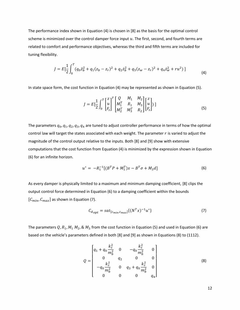
The performance index shown in Equation (4) is chosen in [8] as the basis for the optimal control

scheme is minimized over the control damper force input 𝑢. The first, second, and fourth terms are

related to comfort and performance objectives, whereas the third and fifth terms are included for

tuning flexibility.

𝐽 = 𝐸[

1

2∫ (𝑞0�̈�𝑏

2 + 𝑞1(𝑧𝑏 − 𝑧𝑟)2

𝑇

0

+ 𝑞2�̇�𝑏2 + 𝑞3(𝑧𝑤 − 𝑧𝑟)

2 + 𝑞4�̇�𝑤2 + 𝑟𝑢2) ]

(4)

In state space form, the cost function in Equation (4) may be represented as shown in Equation (5).

𝐽 = 𝐸[

1

2∫ [

𝑧𝑢𝐹𝑠]

𝑇

[

𝑄 𝑀1 𝑀2𝑀1𝑇 𝑅1 𝑀3

𝑀2𝑇 𝑀3

𝑇 𝑅2

] [

𝑧𝑢𝐹𝑠]

𝑇

0

) ]

(5)

The parameters 𝑞0, 𝑞1, 𝑞2, 𝑞3, 𝑞4 are tuned to adjust controller performance in terms of how the optimal

control law will target the states associated with each weight. The parameter 𝑟 is varied to adjust the

magnitude of the control output relative to the inputs. Both [8] and [9] show with extensive

computations that the cost function from Equation (4) is minimized by the expression shown in Equation

(6) for an infinite horizon.

𝑢∗ = −𝑅1

−1[(𝐵𝑇𝑃 +𝑀1𝑇)𝑥 − 𝐵𝑇𝜎 +𝑀3𝑑]

(6)

As every damper is physically limited to a maximum and minimum damping coefficient, [8] clips the

output control force determined in Equation (6) to a damping coefficient within the bounds

[𝐶𝑚𝑖𝑛, 𝐶𝑚𝑎𝑥] as shown in Equation (7).

𝐶𝑑𝑜𝑝𝑡 = 𝑠𝑎𝑡[𝑐𝑚𝑖𝑛,𝑐𝑚𝑎𝑥]{(𝑁

𝑇𝑥)−1𝑢∗}

(7)

The parameters 𝑄, 𝑅1,𝑀1 𝑀2, & 𝑀3 from the cost function in Equation (5) and used in Equation (6) are

based on the vehicle’s parameters defined in both [8] and [9] as shown in Equations (8) to (1112).

𝑄 =

[ 𝑞1 + 𝑞0

𝑘𝑠2

𝑚𝑏2 0 −𝑞0

𝑘𝑠2

𝑚𝑏2 0

0 𝑞2 0 0

−𝑞0𝑘𝑠2

𝑚𝑏2 0 𝑞3 + 𝑞0

𝑘𝑠2

𝑚𝑏2 0

0 0 0 𝑞4]

(8)

13

𝑅1 = [𝑟 +

𝑞0

𝑚𝑏2]𝑁

𝑇𝑁

(9)

𝑀1 = −𝑀2 = [ 𝑞0 (

𝑘𝑠

𝑚𝑏2) 0 −𝑞0 (

𝑘𝑠

𝑚𝑏2) 0]

𝑇

(10)

𝑀3 = −𝑞0

1

𝑚𝑏2

(11)

Controller tuning in this case means choosing desired weighting factors and then determining the

matrices 𝑃 and 𝜎 so Equation (6) may be solved.

The set of terms in Equation (6) that is multiplied by state vector 𝑥 is a feedback term based on vehicle

states. The matrix 𝑃 is determined according to chosen weighting factors in the cost function in

Equation (4). This is done by numerically solving the algebraic Riccati Equation as follows in Equation

(12).

𝑃{𝐴 − 𝐵𝑅−1𝑀1

𝑇} + {𝐴 − 𝐵𝑅−1𝑀1𝑇}𝑇𝑃 − 𝑃𝐵𝑅−1𝐵𝑇𝑃 + {𝑄 −𝑀1𝑅

−1𝑀1𝑇} = 0

(12)

The second term seen in Equation (6) including 𝜎 is a feedforward term based on the inertial forces

subjected to the sprung mass. For a quarter car model, 𝑑 = 𝐹𝑠 as only vertical motion is considered. For

an infinite horizon, [8] determines the matrix 𝜎 from the algebraic Equation shown below in Equation

(13).

[𝐴𝑇 −𝑀1𝑅

−1𝐵𝑇 − 𝑃𝐵𝑅−1𝐵𝑇]𝜎 + [𝑀2 −𝑀1𝑅−1𝑀3 + 𝑃(𝐹 − 𝐵𝑅

−1𝑀3)]𝑑 = 0

(13)

Once both the terms 𝑃 and 𝜎 are determined, controller tuning is complete. At this point, Equation (6)

can be solved in the controller at each time step or sampling increment. This produces an optimal

damper force given the input states and applied loads.

2.2.2. Full Car Ride Model

The above set of Equations are also valid for a full car ride model, which is developed in [9] for optimal

control and applied in [8] for clipped optimal control. As before, displacements are taken relative to the

road input, as in the complete state space derivation of this system referenced in [9]. As with the

14

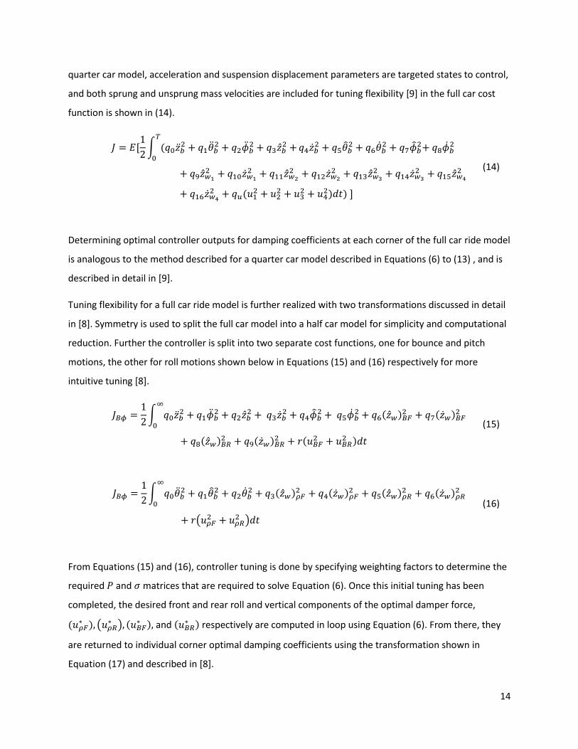
quarter car model, acceleration and suspension displacement parameters are targeted states to control,

and both sprung and unsprung mass velocities are included for tuning flexibility [9] in the full car cost

function is shown in (14).

𝐽 = 𝐸[1

2∫ (𝑞0�̈�𝑏

2 + 𝑞1�̈�𝑏2 + 𝑞2�̈�𝑏

2 + 𝑞3�̂�𝑏2 +

𝑇

0

𝑞4�̇�𝑏2 + 𝑞5�̂�𝑏

2 + 𝑞6�̇�𝑏2 + 𝑞7�̂�𝑏

2+ 𝑞8�̇�𝑏2

+ 𝑞9�̂�𝑤12 + 𝑞10�̇�𝑤1

2 + 𝑞11�̂�𝑤22 + 𝑞12�̇�𝑤2

2 + 𝑞13�̂�𝑤32 + 𝑞14�̇�𝑤3

2 + 𝑞15�̂�𝑤42

+ 𝑞16�̇�𝑤42 + 𝑞𝑢(𝑢1

2 + 𝑢22 + 𝑢3

2 + 𝑢42)𝑑𝑡) ]

(14)

Determining optimal controller outputs for damping coefficients at each corner of the full car ride model

is analogous to the method described for a quarter car model described in Equations (6) to (13) , and is

described in detail in [9].

Tuning flexibility for a full car ride model is further realized with two transformations discussed in detail

in [8]. Symmetry is used to split the full car model into a half car model for simplicity and computational

reduction. Further the controller is split into two separate cost functions, one for bounce and pitch

motions, the other for roll motions shown below in Equations (15) and (16) respectively for more

intuitive tuning [8].

𝐽𝐵𝜙 =

1

2∫ 𝑞0�̈�𝑏

2 + 𝑞1�̈�𝑏2 + 𝑞2�̂�𝑏

2 + 𝑞3�̇�𝑏2 + 𝑞4�̂�𝑏

2 + 𝑞5�̇�𝑏2

∞

0

+ 𝑞6(�̂�𝑤)𝐵𝐹2 + 𝑞7(�̇�𝑤)𝐵𝐹

2

+ 𝑞8(�̂�𝑤)𝐵𝑅2 + 𝑞9(�̇�𝑤)𝐵𝑅

2 + 𝑟(𝑢𝐵𝐹2 + 𝑢𝐵𝑅

2 )𝑑𝑡

(15)

𝐽𝐵𝜙 =

1

2∫ 𝑞0�̈�𝑏

2 + 𝑞1𝜃𝑏2 + 𝑞2�̇�𝑏

2∞

0

+ 𝑞3(�̂�𝑤)𝜌𝐹2 + 𝑞4(�̇�𝑤)𝜌𝐹

2 + 𝑞5(�̂�𝑤)𝜌𝑅2 + 𝑞6(�̇�𝑤)𝜌𝑅

2

+ 𝑟(𝑢𝜌𝐹2 + 𝑢𝜌𝑅

2 )𝑑𝑡

(16)

From Equations (15) and (16), controller tuning is done by specifying weighting factors to determine the

required 𝑃 and 𝜎 matrices that are required to solve Equation (6). Once this initial tuning has been

completed, the desired front and rear roll and vertical components of the optimal damper force,

(𝑢𝜌𝐹∗ ), (𝑢𝜌𝑅

∗ ), (𝑢𝐵𝐹∗ ), and (𝑢𝐵𝑅

∗ ) respectively are computed in loop using Equation (6). From there, they

are returned to individual corner optimal damping coefficients using the transformation shown in

Equation (17) and described in [8].

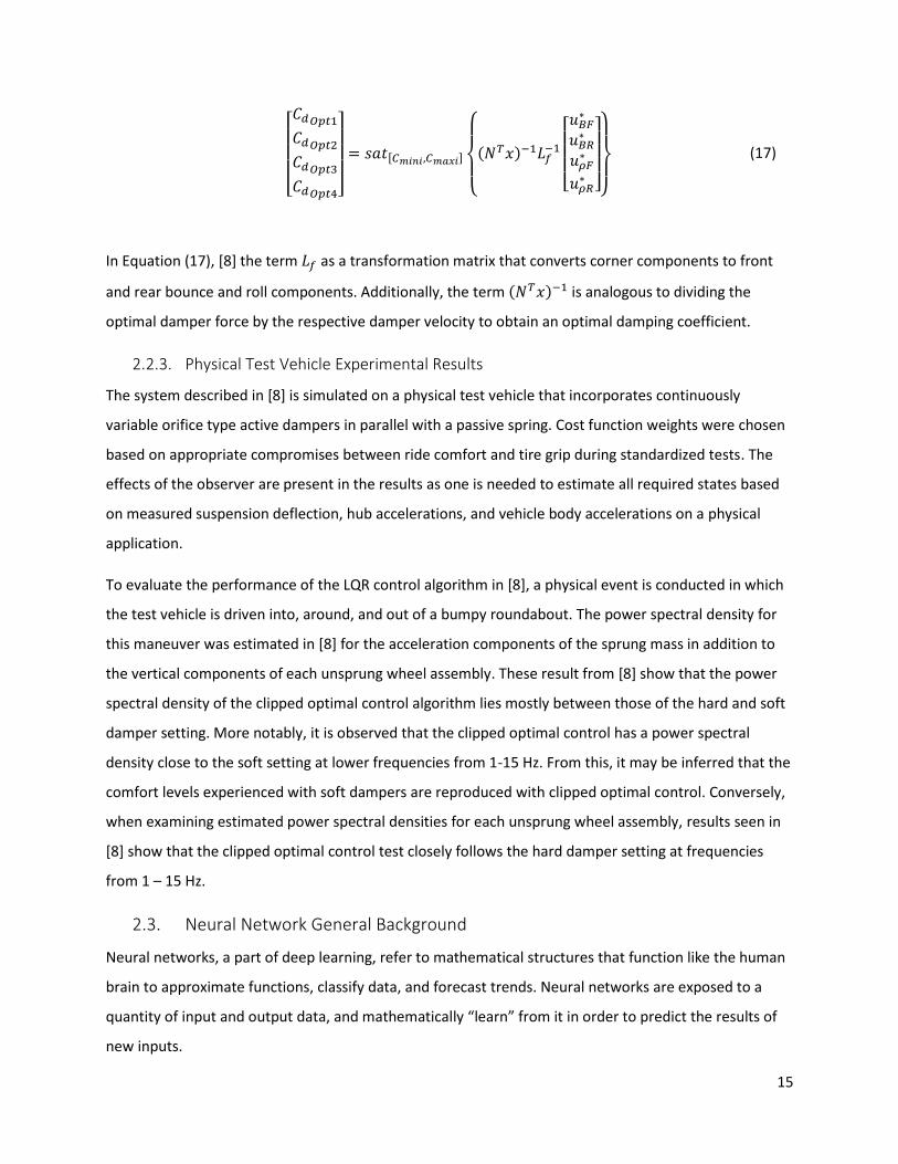
15

[ 𝐶𝑑𝑂𝑝𝑡1𝐶𝑑𝑂𝑝𝑡2𝐶𝑑𝑂𝑝𝑡3𝐶𝑑𝑂𝑝𝑡4]

= 𝑠𝑎𝑡[𝐶𝑚𝑖𝑛𝑖,𝐶𝑚𝑎𝑥𝑖]

{

(𝑁𝑇𝑥)−1𝐿𝑓−1

[ 𝑢𝐵𝐹∗

𝑢𝐵𝑅∗

𝑢𝜌𝐹∗

𝑢𝜌𝑅∗]

}

(17)

In Equation (17), [8] the term 𝐿𝑓 as a transformation matrix that converts corner components to front

and rear bounce and roll components. Additionally, the term (𝑁𝑇𝑥)−1 is analogous to dividing the

optimal damper force by the respective damper velocity to obtain an optimal damping coefficient.

2.2.3. Physical Test Vehicle Experimental Results

The system described in [8] is simulated on a physical test vehicle that incorporates continuously

variable orifice type active dampers in parallel with a passive spring. Cost function weights were chosen

based on appropriate compromises between ride comfort and tire grip during standardized tests. The

effects of the observer are present in the results as one is needed to estimate all required states based

on measured suspension deflection, hub accelerations, and vehicle body accelerations on a physical

application.

To evaluate the performance of the LQR control algorithm in [8], a physical event is conducted in which

the test vehicle is driven into, around, and out of a bumpy roundabout. The power spectral density for

this maneuver was estimated in [8] for the acceleration components of the sprung mass in addition to

the vertical components of each unsprung wheel assembly. These result from [8] show that the power

spectral density of the clipped optimal control algorithm lies mostly between those of the hard and soft

damper setting. More notably, it is observed that the clipped optimal control has a power spectral

density close to the soft setting at lower frequencies from 1-15 Hz. From this, it may be inferred that the

comfort levels experienced with soft dampers are reproduced with clipped optimal control. Conversely,

when examining estimated power spectral densities for each unsprung wheel assembly, results seen in

[8] show that the clipped optimal control test closely follows the hard damper setting at frequencies

from 1 – 15 Hz.

2.3. Neural Network General Background

Neural networks, a part of deep learning, refer to mathematical structures that function like the human

brain to approximate functions, classify data, and forecast trends. Neural networks are exposed to a

quantity of input and output data, and mathematically “learn” from it in order to predict the results of

new inputs.

16

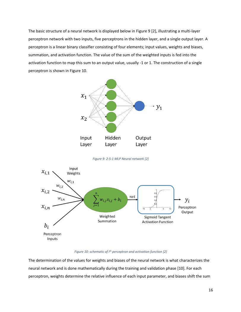
The basic structure of a neural network is displayed below in Figure 9 [2], illustrating a multi-layer

perceptron network with two inputs, five perceptrons in the hidden layer, and a single output layer. A

perceptron is a linear binary classifier consisting of four elements; input values, weights and biases,

summation, and activation function. The value of the sum of the weighted inputs is fed into the

activation function to map this sum to an output value, usually -1 or 1. The construction of a single

perceptron is shown in Figure 10.

Figure 9: 2-5-1 MLP Neural network [2]

Figure 10: schematic of ith perceptron and activation function [2]

The determination of the values for weights and biases of the neural network is what characterizes the

neural network and is done mathematically during the training and validation phase [10]. For each

perceptron, weights determine the relative influence of each input parameter, and biases shift the sum

17

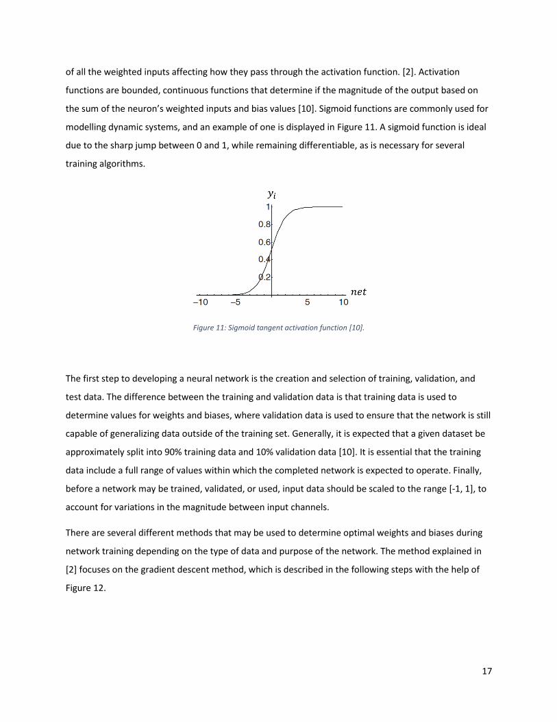
of all the weighted inputs affecting how they pass through the activation function. [2]. Activation

functions are bounded, continuous functions that determine if the magnitude of the output based on

the sum of the neuron’s weighted inputs and bias values [10]. Sigmoid functions are commonly used for

modelling dynamic systems, and an example of one is displayed in Figure 11. A sigmoid function is ideal

due to the sharp jump between 0 and 1, while remaining differentiable, as is necessary for several

training algorithms.

Figure 11: Sigmoid tangent activation function [10].

The first step to developing a neural network is the creation and selection of training, validation, and

test data. The difference between the training and validation data is that training data is used to

determine values for weights and biases, where validation data is used to ensure that the network is still

capable of generalizing data outside of the training set. Generally, it is expected that a given dataset be

approximately split into 90% training data and 10% validation data [10]. It is essential that the training

data include a full range of values within which the completed network is expected to operate. Finally,

before a network may be trained, validated, or used, input data should be scaled to the range [-1, 1], to

account for variations in the magnitude between input channels.

There are several different methods that may be used to determine optimal weights and biases during

network training depending on the type of data and purpose of the network. The method explained in

[2] focuses on the gradient descent method, which is described in the following steps with the help of

Figure 12.

18

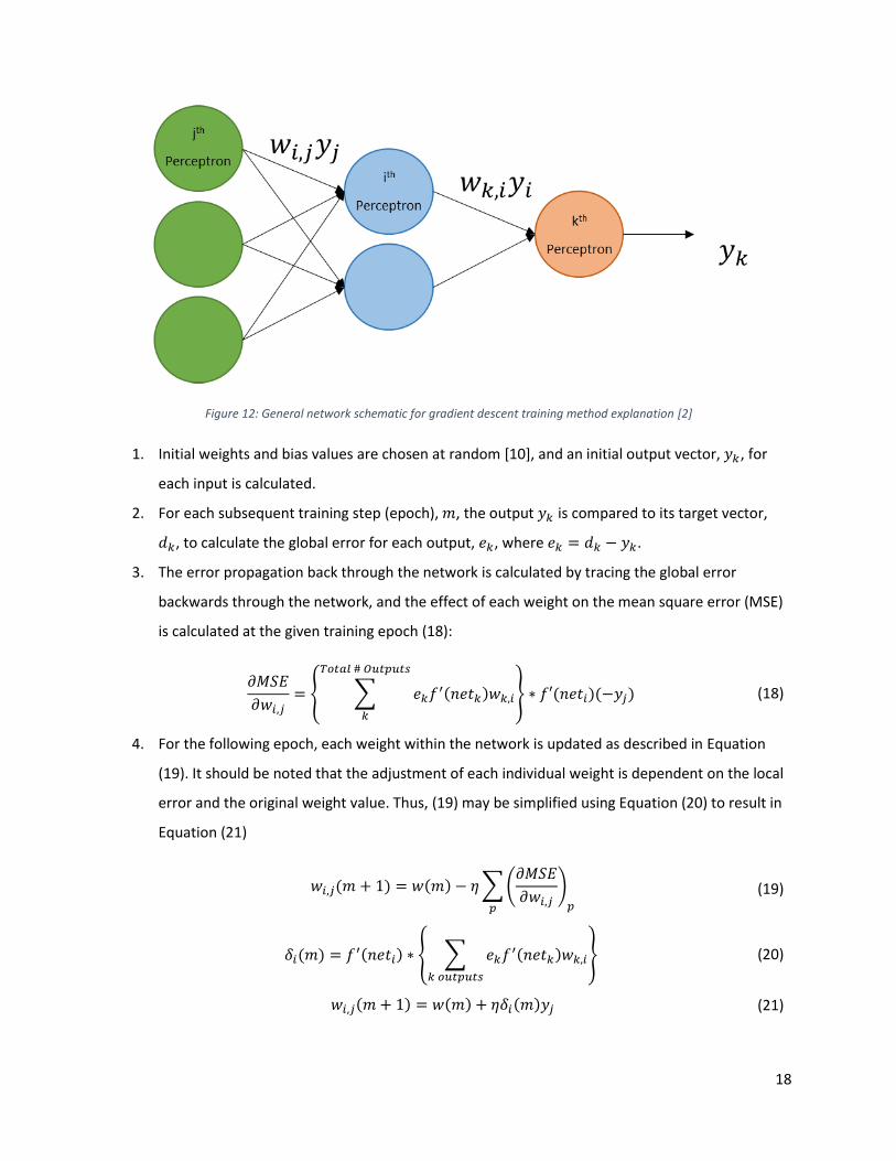
Figure 12: General network schematic for gradient descent training method explanation [2]

1. Initial weights and bias values are chosen at random [10], and an initial output vector, 𝑦𝑘, for

each input is calculated.

2. For each subsequent training step (epoch), 𝑚, the output 𝑦𝑘 is compared to its target vector,

𝑑𝑘, to calculate the global error for each output, 𝑒𝑘, where 𝑒𝑘 = 𝑑𝑘 − 𝑦𝑘.

3. The error propagation back through the network is calculated by tracing the global error

backwards through the network, and the effect of each weight on the mean square error (MSE)

is calculated at the given training epoch (18):

𝜕𝑀𝑆𝐸

𝜕𝑤𝑖,𝑗= { ∑ 𝑒𝑘𝑓

′(𝑛𝑒𝑡𝑘)𝑤𝑘,𝑖

𝑇𝑜𝑡𝑎𝑙 # 𝑂𝑢𝑡𝑝𝑢𝑡𝑠

𝑘

} ∗ 𝑓′(𝑛𝑒𝑡𝑖)(−𝑦𝑗) (18)

4. For the following epoch, each weight within the network is updated as described in Equation

(19). It should be noted that the adjustment of each individual weight is dependent on the local

error and the original weight value. Thus, (19) may be simplified using Equation (20) to result in

Equation (21)

𝑤𝑖,𝑗(𝑚 + 1) = 𝑤(𝑚) − 𝜂∑(𝜕𝑀𝑆𝐸

𝜕𝑤𝑖,𝑗)𝑝𝑝

(19)

𝛿𝑖(𝑚) = 𝑓′(𝑛𝑒𝑡𝑖) ∗ { ∑ 𝑒𝑘𝑓

′(𝑛𝑒𝑡𝑘)𝑤𝑘,𝑖𝑘 𝑜𝑢𝑡𝑝𝑢𝑡𝑠

} (20)

𝑤𝑖,𝑗(𝑚 + 1) = 𝑤(𝑚) + 𝜂𝛿𝑖(𝑚)𝑦𝑗 (21)

19

5. The parameter 𝜂 sets the learning rate of the training algorithm and is set manually in Matlab©

typically around 𝜂 = 0.05. Additionally, the momentum 𝛼 may be included as shown in

Equation (22). This addition serves to consider the rate of change that the weight experienced in

its previous adjustment in the last epoch. Typically, 𝛼 = 0.9.

𝑤𝑖,𝑗(𝑚 + 1) = 𝑤𝑖,𝑗(𝑚) + 𝜂𝛿𝑖(𝑚)𝑦𝑖 + 𝛼{𝑤𝑖,𝑗(𝑚) − 𝑤𝑖,𝑗(𝑚 − 1)} (22)

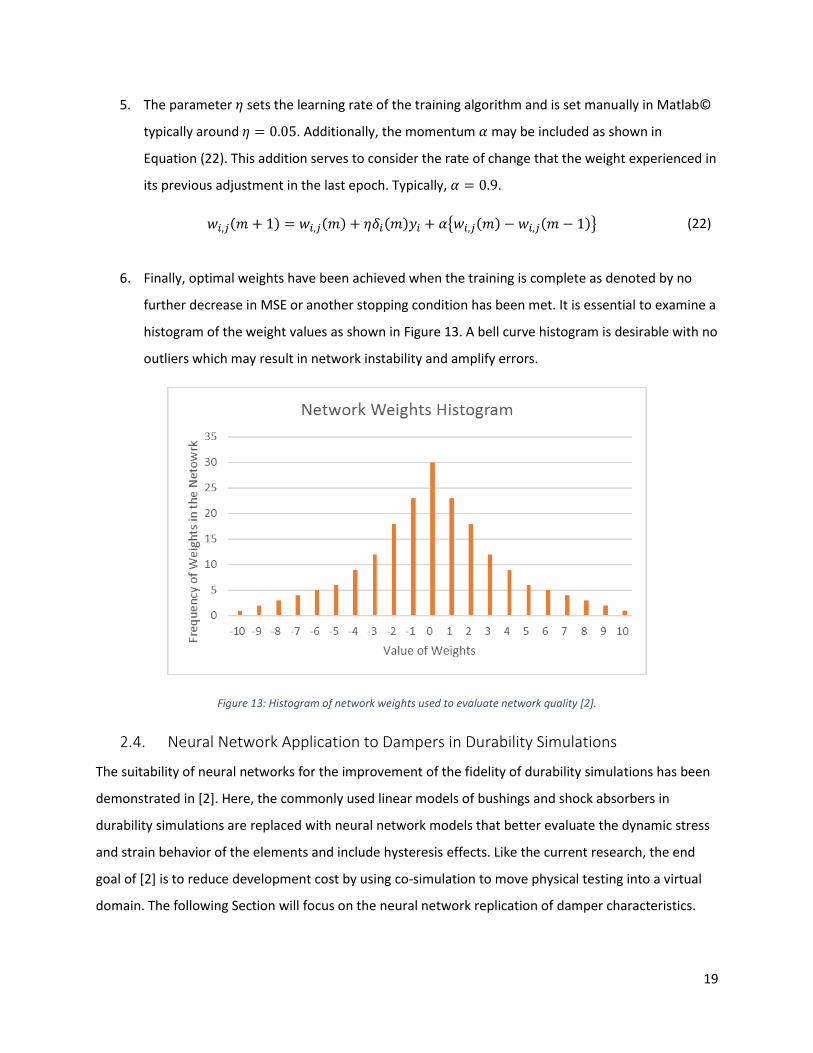
6. Finally, optimal weights have been achieved when the training is complete as denoted by no

further decrease in MSE or another stopping condition has been met. It is essential to examine a

histogram of the weight values as shown in Figure 13. A bell curve histogram is desirable with no

outliers which may result in network instability and amplify errors.

Figure 13: Histogram of network weights used to evaluate network quality [2].

2.4. Neural Network Application to Dampers in Durability Simulations

The suitability of neural networks for the improvement of the fidelity of durability simulations has been

demonstrated in [2]. Here, the commonly used linear models of bushings and shock absorbers in

durability simulations are replaced with neural network models that better evaluate the dynamic stress

and strain behavior of the elements and include hysteresis effects. Like the current research, the end

goal of [2] is to reduce development cost by using co-simulation to move physical testing into a virtual

domain. The following Section will focus on the neural network replication of damper characteristics.

20

To produce an accurate model, it is essential to consider their hysteretic behavior in damper models,

where a current output is dependent on the output of a previous step. An example of hysteric behavior

is shown visually in Figure 3.26 in [2]. To train the neural network to reproduce the hysteretic effects

seen in the measure data, [2] adds two additional inputs for each existing input, containing the

preceding two values of the given input. Networks trained in this fashion are referred to as time delay

neural networks.

2.5. Sliding Mode Control

2.5.1. Controller Construction

A common problem with many of the control systems explored in this work is their dependence on

assumed vehicle parameters when modelling a control system. Sliding Mode Control (SMC) algorithms

have been developed in [11] and [12] that practically implement previously discussed Skyhook control

theory. Both [11] and [12] have very similar construction of their respective sliding mode control

algorithms, which are presented, as is typical, using the standard quarter car model as shown below in

Equations (23) and (24).

𝑚𝑏�̈�𝑏 + 𝑘𝑠(𝑧𝑏 − 𝑧𝑤) + 𝑢 = 0 (23)

𝑚𝑤�̈�𝑤 − 𝑘𝑠(𝑧𝑏 − 𝑧𝑤) + 𝑘𝑡(𝑧𝑤 − 𝑧𝑟) − 𝑢 = 0 (24)

In the above Equations, the term 𝑓𝑎 is the semi active suspension damper force which depends on the

relative damper velocity and the effects of the SMC algorithm described as follows. The first phase of

SMC is to define the sliding surface, 𝑆, which, for a two degree for freedom quarter car model, is

specified in both [11] and [12] as follows:

𝑆 = �̇� + 𝜆𝑒 (25)

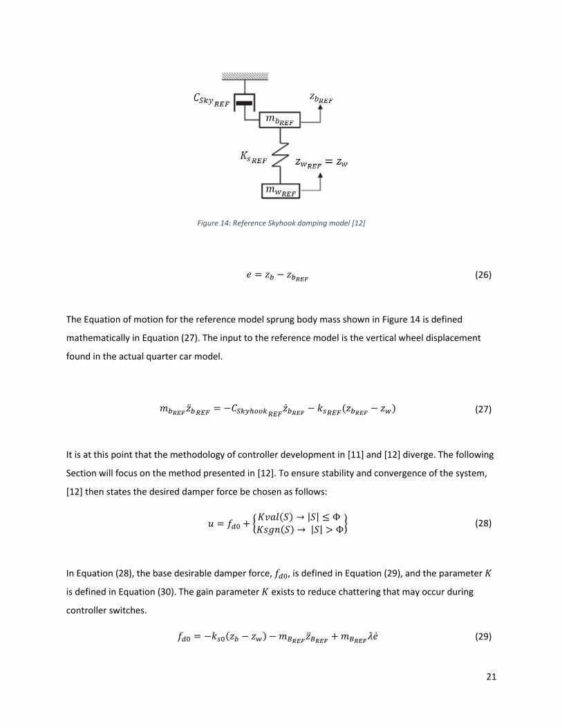
The error value, e, seen above in Equation (25) is defined in Equation (26) as the difference between the

vertical body displacement of the actual vehicle quarter car model and a new reference quarter car

model as seen below in Figure 14. The parameter 𝜆 is a tuning parameter of the controller.

21

Figure 14: Reference Skyhook damping model [12]

𝑒 = 𝑧𝑏 − 𝑧𝑏𝑅𝐸𝐹 (26)

The Equation of motion for the reference model sprung body mass shown in Figure 14 is defined

mathematically in Equation (27). The input to the reference model is the vertical wheel displacement

found in the actual quarter car model.

𝑚𝑏𝑅𝐸𝐹 �̈�𝑏𝑅𝐸𝐹 = −𝐶𝑆𝑘𝑦ℎ𝑜𝑜𝑘𝑅𝐸𝐹�̇�𝑏𝑅𝐸𝐹 − 𝑘𝑠𝑅𝐸𝐹(𝑧𝑏𝑅𝐸𝐹 − 𝑧𝑤) (27)

It is at this point that the methodology of controller development in [11] and [12] diverge. The following

Section will focus on the method presented in [12]. To ensure stability and convergence of the system,

[12] then states the desired damper force be chosen as follows:

𝑢 = 𝑓𝑑0 + {𝐾𝑣𝑎𝑙(𝑆) → |𝑆| ≤ Φ 𝐾𝑠𝑔𝑛(𝑆) → |𝑆| > Φ

} (28)

In Equation (28), the base desirable damper force, 𝑓𝑑0, is defined in Equation (29), and the parameter 𝐾

is defined in Equation (30). The gain parameter 𝐾 exists to reduce chattering that may occur during

controller switches.

𝑓𝑑0 = −𝑘𝑠0(𝑧𝑏 − 𝑧𝑤) − 𝑚𝐵𝑅𝐸𝐹 �̈�𝐵𝑅𝐸𝐹 +𝑚𝐵𝑅𝐸𝐹𝜆�̇� (29)

22

𝐾 = (𝜇 − 1){|𝑓𝑑0| + 𝑘𝑠0|𝑧𝑏| + 𝑘𝑠0|𝑧𝑤|} + 𝑚𝐵𝑅𝐸𝐹𝜇𝜖 (30)

A common issue seen with several controllers is their lack of robustness due to their dependence on

knowing vehicle parameters that are subject to change depending on use, specifically the vehicle mass

for the case of a quarter car model. To account for this, the parameter 𝜇 is used to determine the

allowable limits on the ratio between the actual vehicle mass 𝑚𝑏 and the reference vehicle model mass

𝑚𝑏𝑅𝐸𝐹. As such, 𝜇 is defined using Equation (31).

1

𝜇≤

𝑚𝑏

𝑚𝑏𝑅𝐸𝐹 ≤ 𝜇 (31)

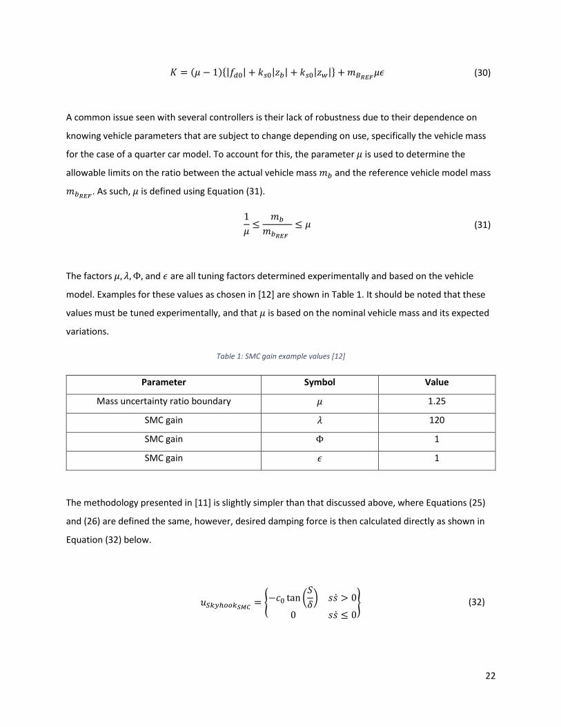
The factors 𝜇, 𝜆,Φ, and 𝜖 are all tuning factors determined experimentally and based on the vehicle

model. Examples for these values as chosen in [12] are shown in Table 1. It should be noted that these

values must be tuned experimentally, and that 𝜇 is based on the nominal vehicle mass and its expected

variations.

Table 1: SMC gain example values [12]

Parameter Symbol Value

Mass uncertainty ratio boundary 𝜇 1.25

SMC gain 𝜆 120

SMC gain Φ 1

SMC gain 𝜖 1

The methodology presented in [11] is slightly simpler than that discussed above, where Equations (25)

and (26) are defined the same, however, desired damping force is then calculated directly as shown in

Equation (32) below.

𝑢𝑆𝑘𝑦ℎ𝑜𝑜𝑘𝑆𝑀𝐶 = {−𝑐0 tan (

𝑆

𝛿) 𝑠�̇� > 0

0 𝑠�̇� ≤ 0} (32)

23

In this case, 𝛿 shown above is positive constant denoting the thickness of the sliding mode boundary

layer. In [11] tuning constants are defined as 𝛿 = 28.1569 and 𝜆 = 10.6341 for the quarter car

controller presented.

It should be noted that the main differences seen between different literature resources on the subject

of semi – active suspension sliding mode control are the way that the gain 𝐾 in Equation (28) and the

final output damper force 𝑓𝑑 in Equation (30) are calculated. Another differently presented method to

the two described above may be found in [13].

2.5.2. Simulation Results

A Sliding Mode Controller (SMC) was constructed in Matlab© / Simulink© in [11] and its effects on a

quarter car model travelling over an ISO 2631 Class C stochastic road profile are compared to a fuzzy

logic controller (FLC) and passive suspension. This comparison was chosen due to the inherent robust

characteristics of fuzzy logic. Results from [11] show that the sliding mode controller greatly

outperforms the fuzzy logic controller in terms of vertical body acceleration, a common metric for

evaluating ride comfort.

24

3. Controller Development

3.1. Clipped Optimal Controller Development

3.1.1. Matlab© Quarter Car

An initial analysis of the performance of a clipped optimal controller is performed in Matlab© and

Simulink© concerning only a quarter car model. The physical parameters of the quarter car model are

from [12]. The controller is modeled in Matlab© using concepts outlined in [8].

3.1.1.1. Quarter Car Controller Development

The methodology presented in [8] and [9] is develops a clipped optimal controller based on the state

space representation of a quarter car model. To easily adapt this to Simulink©, all required state space

Equations are created in a Simulink© user defined function block, which is written as a regular Matlab©

function.

The Simulink© block accepts all necessary states to complete the state variable 𝑋 seen in Equation (3)

from the quarter car model. With these inputs, Equation (6) may be solved, and based on the input

damper velocity, a clipped optimal damping coefficient is calculated from Equation (7). Finally, the

resulting optimal damper coefficient and damper velocity is used to return an optimal damper force to

the Simulink© workspace to be fed back to the quarter car model.

The simplified implementation of the Simulink© block is shown interacting with a quarter car model in

Figure 15.

25

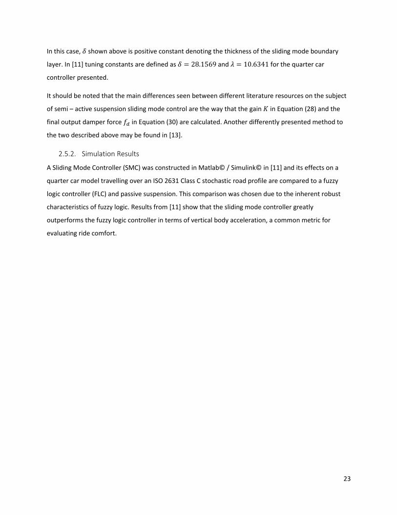
Figure 15: Simulink© Optimal controller and quarter car model diagram

Before the block may be implemented in a simulation, it is necessary to determine the constant matrices

used in Equation (6). This is done with a separate Matlab© script which solves the algebraic Riccati

Equation shown in Equation (12) and Equation (13) for matrices 𝑃 and 𝜎 respectively. Additionally,

matrices 𝑀1,𝑀3 and 𝑅1 must be predetermined from Equations (10), (11) and (9) respectively. These

values are then read from the workspace and fed to the Simulink© controller block as constants during

simulation as shown above in Figure 15.

3.1.1.2. Quarter Car Simulink© Implementation

A quarter car model is used to perform an initial analysis of the clipped optimal controller described

above. The parameters for the quarter car model are taken from [12], and it is excited using a standard

ISO 8608 D-class stochastic road profile from [14]. Controller weights displayed in Table 2 are selected

based on recommendations in [9] and from some fine adjustment to suit the given quarter car model.

26

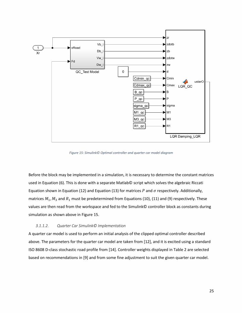
Table 2: Clipped optimal controller tuning weights

Weight Cost Function Parameter Value

𝑞0 �̈�𝑏 105

𝑞1 𝑧𝑏 − 𝑧𝑟 109

𝑞2 �̇�𝑏 106

𝑞3 𝑧𝑤 − 𝑧𝑟 108

𝑞4 �̇�𝑤 104

𝑟 𝑢 1

The resulting time history output of vertical body acceleration and output damper force are shown in

Figure 16 and Figure 17 respectively. Included in each is a relative plot of a quarter car model

implemented with only the passive damping coefficient given in [12].

Figure 16: Time domain plot of vertical sprung body acceleration of quarter car models with clipped optimal controlled and

passive damping

27

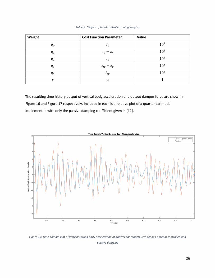
Figure 17: Time domain plot of damper force of quarter car models with clipped optimal controlled and passive damping

Immediately apparent from Figure 16 is the reduction in accelerations experienced by the sprung body

mass when the clipped optimal controller is implemented. For this demonstration, the tuning

coefficient 𝑞0, targeting the vertical acceleration of the sprung body mass, was selected as in Table 2 to

provide the acceleration reduced results shown above. In real applications, all tuning weights must be

adjusted to meet a given compromise of vehicle suspension performance.

In Figure 17, the output damper force from the clipped optimal controller is lower than the passive

damping for the majority of the displayed time. This exhibits an inherent characteristic of LQR control

design. Because the optimal controller has been designed to reduce body acceleration as discussed

above the optimal damping for this performance objective is often the softest setting. Because the soft

damping coefficient used in this demonstration is less than the passive one, output damping force is also

of lesser magnitude. This fact however does not imply that the clipped optimal controller merely assigns

the softest damping setting at all times as occasional switches to a harder setting are visible in Figure 17

by discontinuities in the curve.

An amplitude spectrum the vertical body acceleration is also estimated over a sine sweep input to

produce Figure 18.

28

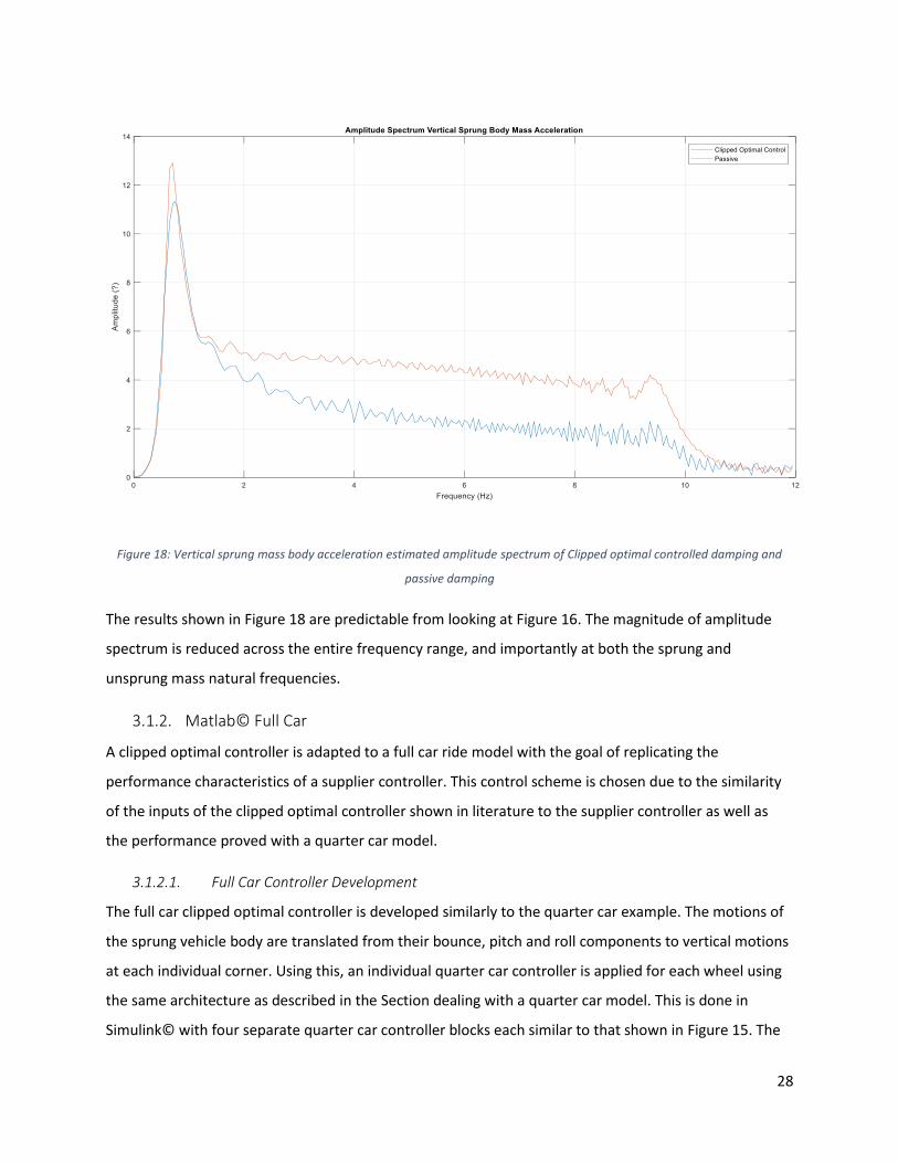
Figure 18: Vertical sprung mass body acceleration estimated amplitude spectrum of Clipped optimal controlled damping and

passive damping

The results shown in Figure 18 are predictable from looking at Figure 16. The magnitude of amplitude

spectrum is reduced across the entire frequency range, and importantly at both the sprung and

unsprung mass natural frequencies.

3.1.2. Matlab© Full Car

A clipped optimal controller is adapted to a full car ride model with the goal of replicating the

performance characteristics of a supplier controller. This control scheme is chosen due to the similarity

of the inputs of the clipped optimal controller shown in literature to the supplier controller as well as

the performance proved with a quarter car model.

3.1.2.1. Full Car Controller Development

The full car clipped optimal controller is developed similarly to the quarter car example. The motions of

the sprung vehicle body are translated from their bounce, pitch and roll components to vertical motions

at each individual corner. Using this, an individual quarter car controller is applied for each wheel using

the same architecture as described in the Section dealing with a quarter car model. This is done in

Simulink© with four separate quarter car controller blocks each similar to that shown in Figure 15. The

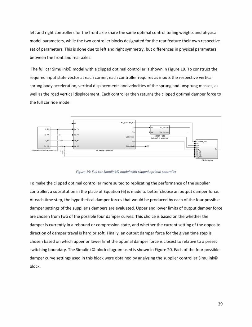
29

left and right controllers for the front axle share the same optimal control tuning weights and physical

model parameters, while the two controller blocks designated for the rear feature their own respective

set of parameters. This is done due to left and right symmetry, but differences in physical parameters

between the front and rear axles.

The full car Simulink© model with a clipped optimal controller is shown in Figure 19. To construct the

required input state vector at each corner, each controller requires as inputs the respective vertical

sprung body acceleration, vertical displacements and velocities of the sprung and unsprung masses, as

well as the road vertical displacement. Each controller then returns the clipped optimal damper force to

the full car ride model.

Figure 19: Full car Simulink© model with clipped optimal controller

To make the clipped optimal controller more suited to replicating the performance of the supplier

controller, a substitution in the place of Equation (6) is made to better choose an output damper force.

At each time step, the hypothetical damper forces that would be produced by each of the four possible

damper settings of the supplier’s dampers are evaluated. Upper and lower limits of output damper force

are chosen from two of the possible four damper curves. This choice is based on the whether the

damper is currently in a rebound or compression state, and whether the current setting of the opposite

direction of damper travel is hard or soft. Finally, an output damper force for the given time step is

chosen based on which upper or lower limit the optimal damper force is closest to relative to a preset

switching boundary. The Simulink© block diagram used is shown in Figure 20. Each of the four possible

damper curve settings used in this block were obtained by analyzing the supplier controller Simulink©

block.

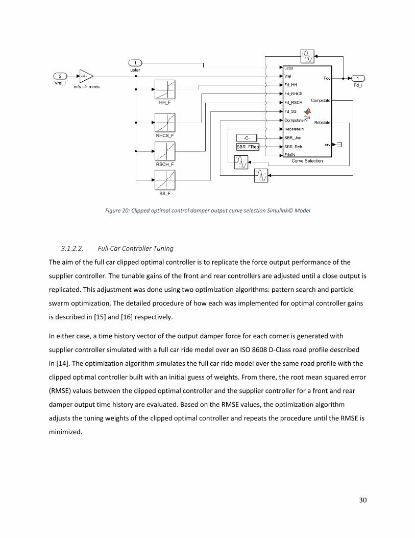
30

Figure 20: Clipped optimal control damper output curve selection Simulink© Model

3.1.2.2. Full Car Controller Tuning

The aim of the full car clipped optimal controller is to replicate the force output performance of the

supplier controller. The tunable gains of the front and rear controllers are adjusted until a close output is

replicated. This adjustment was done using two optimization algorithms: pattern search and particle

swarm optimization. The detailed procedure of how each was implemented for optimal controller gains

is described in [15] and [16] respectively.

In either case, a time history vector of the output damper force for each corner is generated with

supplier controller simulated with a full car ride model over an ISO 8608 D-Class road profile described

in [14]. The optimization algorithm simulates the full car ride model over the same road profile with the

clipped optimal controller built with an initial guess of weights. From there, the root mean squared error

(RMSE) values between the clipped optimal controller and the supplier controller for a front and rear

damper output time history are evaluated. Based on the RMSE values, the optimization algorithm

adjusts the tuning weights of the clipped optimal controller and repeats the procedure until the RMSE is

minimized.

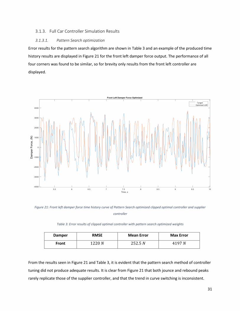
31

3.1.3. Full Car Controller Simulation Results

3.1.3.1. Pattern Search optimization

Error results for the pattern search algorithm are shown in Table 3 and an example of the produced time

history results are displayed in Figure 21 for the front left damper force output. The performance of all

four corners was found to be similar, so for brevity only results from the front left controller are

displayed.

Figure 21: Front left damper force time history curve of Pattern Search optimized clipped optimal controller and supplier

controller

Table 3: Error results of clipped optimal controller with pattern search optimized weights

Damper RMSE Mean Error Max Error

Front 1220 𝑁 252.5 𝑁 4197 𝑁

From the results seen in Figure 21 and Table 3, it is evident that the pattern search method of controller

tuning did not produce adequate results. It is clear from Figure 21 that both jounce and rebound peaks

rarely replicate those of the supplier controller, and that the trend in curve switching is inconsistent.

Target

Dam

per F

orce

, (N

)

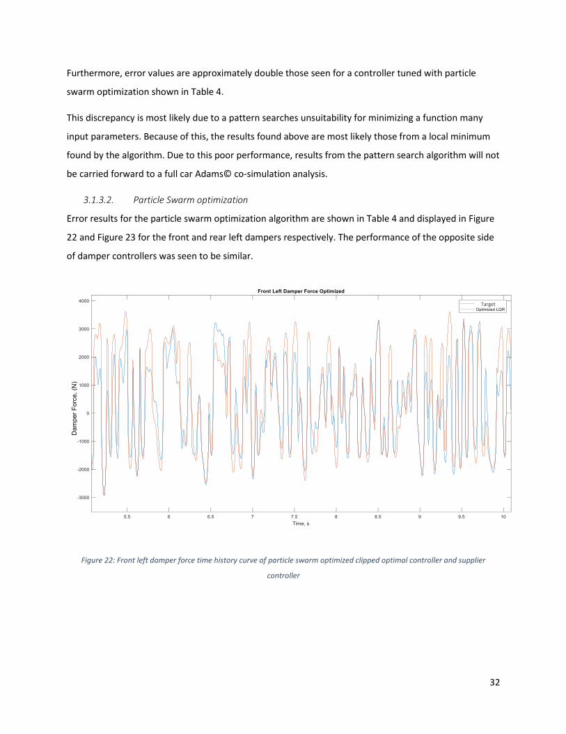
32

Furthermore, error values are approximately double those seen for a controller tuned with particle

swarm optimization shown in Table 4.

This discrepancy is most likely due to a pattern searches unsuitability for minimizing a function many

input parameters. Because of this, the results found above are most likely those from a local minimum

found by the algorithm. Due to this poor performance, results from the pattern search algorithm will not

be carried forward to a full car Adams© co-simulation analysis.

3.1.3.2. Particle Swarm optimization

Error results for the particle swarm optimization algorithm are shown in Table 4 and displayed in Figure

22 and Figure 23 for the front and rear left dampers respectively. The performance of the opposite side

of damper controllers was seen to be similar.

Figure 22: Front left damper force time history curve of particle swarm optimized clipped optimal controller and supplier

controller

Target

Dam

per F

orce

, (N

)

33

Figure 23: Rear left damper force time history curve of particle swarm optimized clipped optimal controller and supplier

controller

Table 4: Error results of clipped optimal controller with particle swarm optimized weights

Damper RMSE Mean Error Max Error

Front 705.4 𝑁 125.7 𝑁 3223 𝑁

Rear 642.2 𝑁 184.2 𝑁 2680 𝑁

Unfortunately, the clipped optimal controller failed to perfectly match the output performance of the

damper force produced by the supplier controller when weights were tuned with a particle swarm

optimization procedure. At several instances in both Figure 22 and Figure 23, the clipped optimal

controller fails to match the peaks of rebound force exerted by the supplier controller. This is

detrimental due to peak values being of large concern in durability simulations. Additionally, a few

localized chattering events may be noticed in Figure 23.

Despite the above, jounce values as well as the frequency of the response appear to be typically well

matched, and the particle swarm optimization algorithm provided the best performing RMSE values for

clipped optimal control. This optimization algorithm most likely performed better than the

Target

Dam

per F

orce

, (N

)

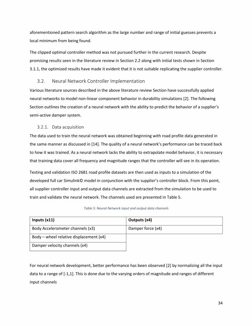
34

aforementioned pattern search algorithm as the large number and range of initial guesses prevents a

local minimum from being found.

The clipped optimal controller method was not pursued further in the current research. Despite

promising results seen in the literature review in Section 2.2 along with initial tests shown in Section

3.1.1, the optimized results have made it evident that it is not suitable replicating the supplier controller.

3.2. Neural Network Controller Implementation

Various literature sources described in the above literature review Section have successfully applied

neural networks to model non-linear component behavior in durability simulations [2]. The following

Section outlines the creation of a neural network with the ability to predict the behavior of a supplier’s

semi-active damper system.

3.2.1. Data acquisition

The data used to train the neural network was obtained beginning with road profile data generated in

the same manner as discussed in [14]. The quality of a neural network’s performance can be traced back

to how it was trained. As a neural network lacks the ability to extrapolate model behavior, it is necessary

that training data cover all frequency and magnitude ranges that the controller will see in its operation.

Testing and validation ISO 2681 road profile datasets are then used as inputs to a simulation of the

developed full car Simulink© model in conjunction with the supplier’s controller block. From this point,

all supplier controller input and output data channels are extracted from the simulation to be used to

train and validate the neural network. The channels used are presented in Table 5.

Table 5: Neural Network input and output data channels

Inputs (x11) Outputs (x4)

Body Accelerometer channels (x3) Damper force (x4)

Body – wheel relative displacement (x4)

Damper velocity channels (x4)

For neural network development, better performance has been observed [2] by normalizing all the input

data to a range of [-1,1]. This is done due to the varying orders of magnitude and ranges of different

input channels

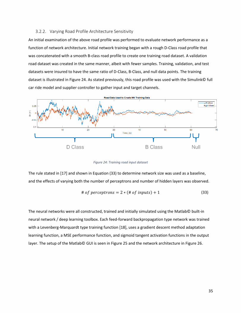
35

3.2.2. Varying Road Profile Architecture Sensitivity

An initial examination of the above road profile was performed to evaluate network performance as a

function of network architecture. Initial network training began with a rough D-Class road profile that

was concatenated with a smooth B-class road profile to create one training road dataset. A validation

road dataset was created in the same manner, albeit with fewer samples. Training, validation, and test

datasets were insured to have the same ratio of D-Class, B-Class, and null data points. The training

dataset is illustrated in Figure 24. As stated previously, this road profile was used with the Simulink© full

car ride model and supplier controller to gather input and target channels.

Figure 24: Training road input dataset

The rule stated in [17] and shown in Equation (33) to determine network size was used as a baseline,

and the effects of varying both the number of perceptrons and number of hidden layers was observed.

# 𝑜𝑓 𝑝𝑒𝑟𝑐𝑒𝑝𝑡𝑟𝑜𝑛𝑠 = 2 ∗ (# 𝑜𝑓 𝑖𝑛𝑝𝑢𝑡𝑠) + 1 (33)

The neural networks were all constructed, trained and initially simulated using the Matlab© built-in

neural network / deep learning toolbox. Each feed-forward backpropagation type network was trained

with a Levenberg-Marquardt type training function [18], uses a gradient descent method adaptation

learning function, a MSE performance function, and sigmoid tangent activation functions in the output

layer. The setup of the Matlab© GUI is seen in Figure 25 and the network architecture in Figure 26.

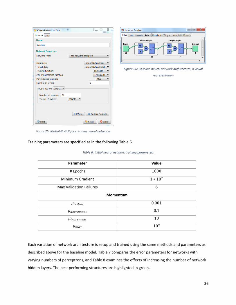
36

Figure 25: Matlab© GUI for creating neural networks

Figure 26: Baseline neural network architecture, a visual

representation

Training parameters are specified as in the following Table 6.

Table 6: Initial neural network training parameters

Parameter Value

# Epochs 1000

Minimum Gradient 1 ∗ 107

Max Validation Failures 6

Momentum

𝜇𝑖𝑛𝑖𝑡𝑖𝑎𝑙 0.001

𝜇𝑑𝑒𝑐𝑟𝑒𝑚𝑒𝑛𝑡 0.1

𝜇𝑖𝑛𝑐𝑟𝑒𝑚𝑒𝑛𝑡 10

𝜇𝑚𝑎𝑥 109

Each variation of network architecture is setup and trained using the same methods and parameters as

described above for the baseline model. Table 7 compares the error parameters for networks with

varying numbers of perceptrons, and Table 8 examines the effects of increasing the number of network

hidden layers. The best performing structures are highlighted in green.

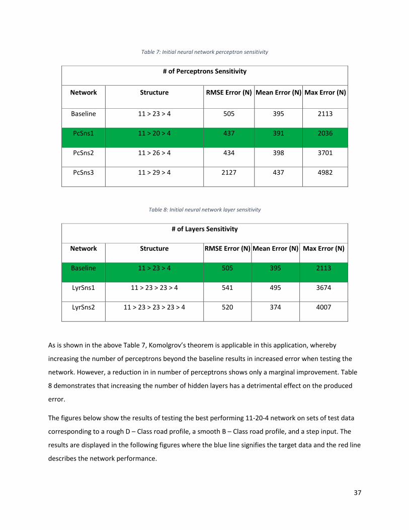
37

Table 7: Initial neural network perceptron sensitivity

# of Perceptrons Sensitivity

Network Structure RMSE Error (N) Mean Error (N) Max Error (N)

Baseline 11 > 23 > 4 505 395 2113

PcSns1 11 > 20 > 4 437 391 2036

PcSns2 11 > 26 > 4 434 398 3701

PcSns3 11 > 29 > 4 2127 437 4982

Table 8: Initial neural network layer sensitivity

# of Layers Sensitivity

Network Structure RMSE Error (N) Mean Error (N) Max Error (N)

Baseline 11 > 23 > 4 505 395 2113

LyrSns1 11 > 23 > 23 > 4 541 495 3674

LyrSns2 11 > 23 > 23 > 23 > 4 520 374 4007

As is shown in the above Table 7, Komolgrov’s theorem is applicable in this application, whereby

increasing the number of perceptrons beyond the baseline results in increased error when testing the

network. However, a reduction in in number of perceptrons shows only a marginal improvement. Table

8 demonstrates that increasing the number of hidden layers has a detrimental effect on the produced

error.

The figures below show the results of testing the best performing 11-20-4 network on sets of test data

corresponding to a rough D – Class road profile, a smooth B – Class road profile, and a step input. The

results are displayed in the following figures where the blue line signifies the target data and the red line

describes the network performance.

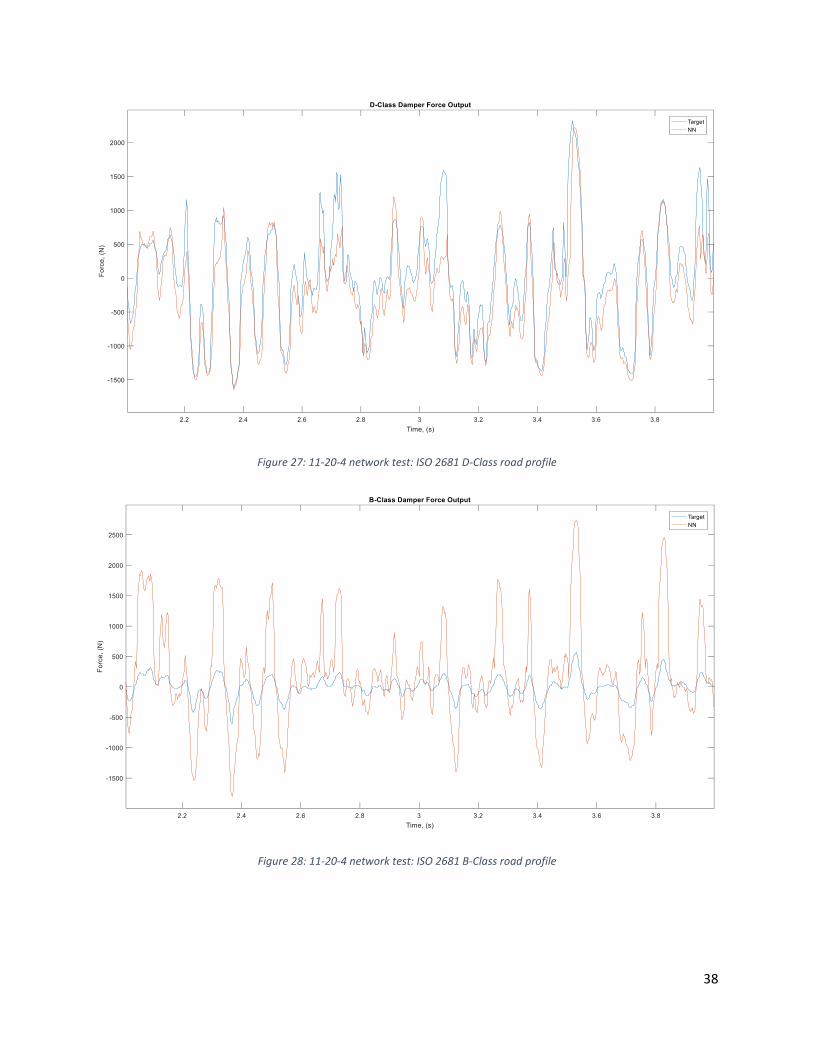
38

Figure 27: 11-20-4 network test: ISO 2681 D-Class road profile

Figure 28: 11-20-4 network test: ISO 2681 B-Class road profile

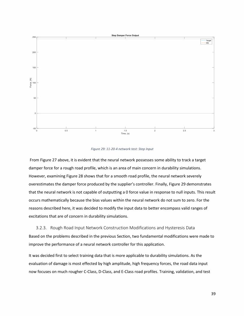
39

Figure 29: 11-20-4 network test: Step Input

From Figure 27 above, it is evident that the neural network possesses some ability to track a target

damper force for a rough road profile, which is an area of main concern in durability simulations.

However, examining Figure 28 shows that for a smooth road profile, the neural network severely

overestimates the damper force produced by the supplier’s controller. Finally, Figure 29 demonstrates

that the neural network is not capable of outputting a 0 force value in response to null inputs. This result

occurs mathematically because the bias values within the neural network do not sum to zero. For the

reasons described here, it was decided to modify the input data to better encompass valid ranges of

excitations that are of concern in durability simulations.

3.2.3. Rough Road Input Network Construction Modifications and Hysteresis Data

Based on the problems described in the previous Section, two fundamental modifications were made to

improve the performance of a neural network controller for this application.

It was decided first to select training data that is more applicable to durability simulations. As the

evaluation of damage is most effected by high amplitude, high frequency forces, the road data input

now focuses on much rougher C-Class, D-Class, and E-Class road profiles. Training, validation, and test

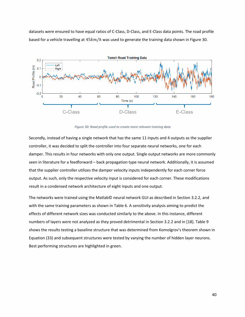
40

datasets were ensured to have equal ratios of C-Class, D-Class, and E-Class data points. The road profile

based for a vehicle travelling at 45𝑘𝑚/ℎ was used to generate the training data shown in Figure 30.

Figure 30: Road profile used to create more relevant training data

Secondly, instead of having a single network that has the same 11 inputs and 4 outputs as the supplier

controller, it was decided to split the controller into four separate neural networks, one for each

damper. This results in four networks with only one output. Single output networks are more commonly

seen in literature for a feedforward – back propagation type neural network. Additionally, it is assumed

that the supplier controller utilizes the damper velocity inputs independently for each corner force

output. As such, only the respective velocity input is considered for each corner. These modifications

result in a condensed network architecture of eight inputs and one output.

The networks were trained using the Matlab© neural network GUI as described in Section 3.2.2, and

with the same training parameters as shown in Table 6. A sensitivity analysis aiming to predict the

effects of different network sizes was conducted similarly to the above. In this instance, different

numbers of layers were not analyzed as they proved detrimental in Section 3.2.2 and in [18]. Table 9

shows the results testing a baseline structure that was determined from Komolgrov’s theorem shown in

Equation (33) and subsequent structures were tested by varying the number of hidden layer neurons.

Best performing structures are highlighted in green.

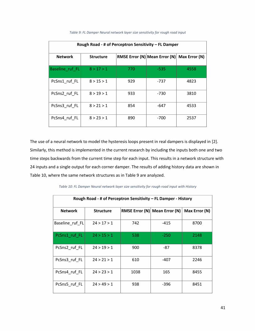
41

Table 9: FL Damper Neural network layer size sensitivity for rough road input

Rough Road - # of Perceptron Sensitivity – FL Damper

Network Structure RMSE Error (N) Mean Error (N) Max Error (N)

Baseline_ruf_FL 8 > 17 > 1 770 -535 4558

PcSns1_ruf_FL 8 > 15 > 1 929 -737 4823

PcSns2_ruf_FL 8 > 19 > 1 933 -730 3810

PcSns3_ruf_FL 8 > 21 > 1 854 -647 4533

PcSns4_ruf_FL 8 > 23 > 1 890 -700 2537

The use of a neural network to model the hysteresis loops present in real dampers is displayed in [2].

Similarly, this method is implemented in the current research by including the inputs both one and two

time steps backwards from the current time step for each input. This results in a network structure with

24 inputs and a single output for each corner damper. The results of adding history data are shown in

Table 10, where the same network structures as in Table 9 are analyzed.

Table 10: FL Damper Neural network layer size sensitivity for rough road input with History

Rough Road - # of Perceptron Sensitivity – FL Damper - History

Network Structure RMSE Error (N) Mean Error (N) Max Error (N)

Baseline_ruf_FL 24 > 17 > 1 742 -415 8700

PcSns1_ruf_FL 24 > 15 > 1 538 -250 2148

PcSns2_ruf_FL 24 > 19 > 1 900 -87 8378

PcSns3_ruf_FL 24 > 21 > 1 610 -407 2246

PcSns4_ruf_FL 24 > 23 > 1 1038 165 8455

PcSns5_ruf_FL 24 > 49 > 1 938 -396 8451

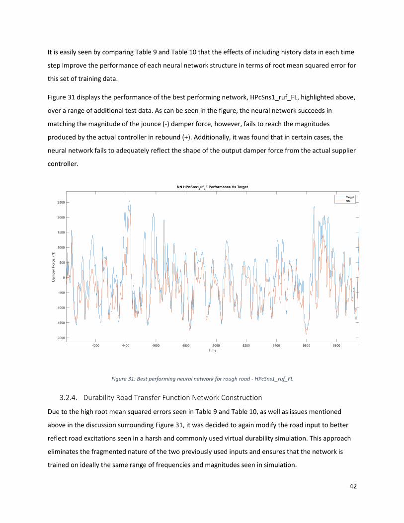
42

It is easily seen by comparing Table 9 and Table 10 that the effects of including history data in each time

step improve the performance of each neural network structure in terms of root mean squared error for

this set of training data.

Figure 31 displays the performance of the best performing network, HPcSns1_ruf_FL, highlighted above,

over a range of additional test data. As can be seen in the figure, the neural network succeeds in

matching the magnitude of the jounce (-) damper force, however, fails to reach the magnitudes

produced by the actual controller in rebound (+). Additionally, it was found that in certain cases, the

neural network fails to adequately reflect the shape of the output damper force from the actual supplier

controller.

Figure 31: Best performing neural network for rough road - HPcSns1_ruf_FL

3.2.4. Durability Road Transfer Function Network Construction

Due to the high root mean squared errors seen in Table 9 and Table 10, as well as issues mentioned

above in the discussion surrounding Figure 31, it was decided to again modify the road input to better

reflect road excitations seen in a harsh and commonly used virtual durability simulation. This approach

eliminates the fragmented nature of the two previously used inputs and ensures that the network is

trained on ideally the same range of frequencies and magnitudes seen in simulation.

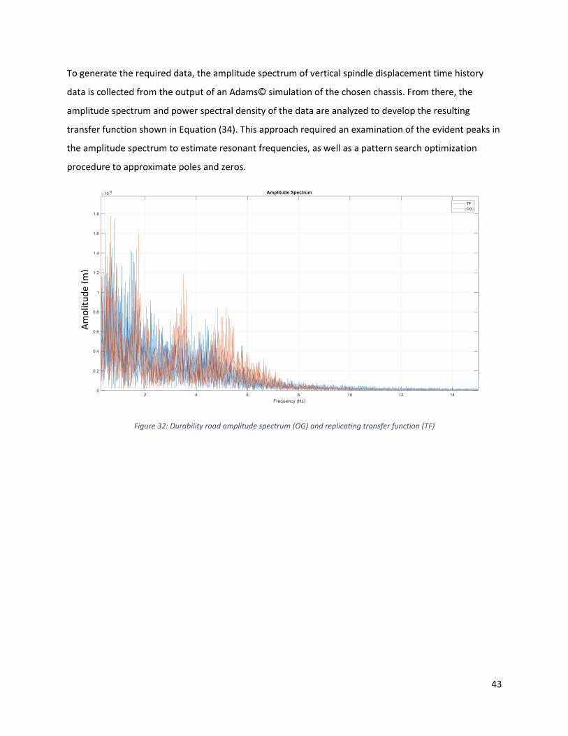
43

To generate the required data, the amplitude spectrum of vertical spindle displacement time history

data is collected from the output of an Adams© simulation of the chosen chassis. From there, the

amplitude spectrum and power spectral density of the data are analyzed to develop the resulting

transfer function shown in Equation (34). This approach required an examination of the evident peaks in

the amplitude spectrum to estimate resonant frequencies, as well as a pattern search optimization

procedure to approximate poles and zeros.

Figure 32: Durability road amplitude spectrum (OG) and replicating transfer function (TF)

Am

plit

ud

e (m

)

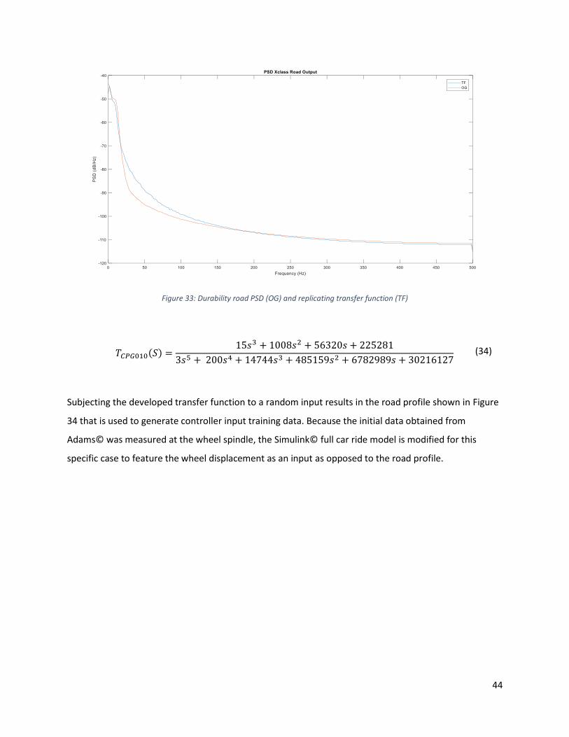
44

Figure 33: Durability road PSD (OG) and replicating transfer function (TF)

𝑇𝐶𝑃𝐺010(𝑆) =15𝑠3 + 1008𝑠2 + 56320𝑠 + 225281

3𝑠5 + 200𝑠4 + 14744𝑠3 + 485159𝑠2 + 6782989𝑠 + 30216127 (34)

Subjecting the developed transfer function to a random input results in the road profile shown in Figure

34 that is used to generate controller input training data. Because the initial data obtained from

Adams© was measured at the wheel spindle, the Simulink© full car ride model is modified for this

specific case to feature the wheel displacement as an input as opposed to the road profile.

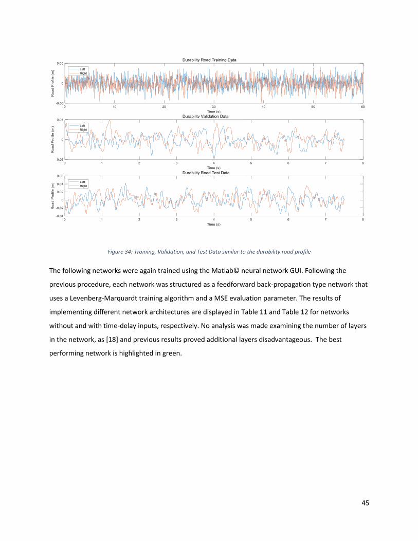
45

Figure 34: Training, Validation, and Test Data similar to the durability road profile

The following networks were again trained using the Matlab© neural network GUI. Following the

previous procedure, each network was structured as a feedforward back-propagation type network that

uses a Levenberg-Marquardt training algorithm and a MSE evaluation parameter. The results of

implementing different network architectures are displayed in Table 11 and Table 12 for networks

without and with time-delay inputs, respectively. No analysis was made examining the number of layers

in the network, as [18] and previous results proved additional layers disadvantageous. The best

performing network is highlighted in green.

Durability Road Training Data

Durability Road Test Data

Durability Validation Data

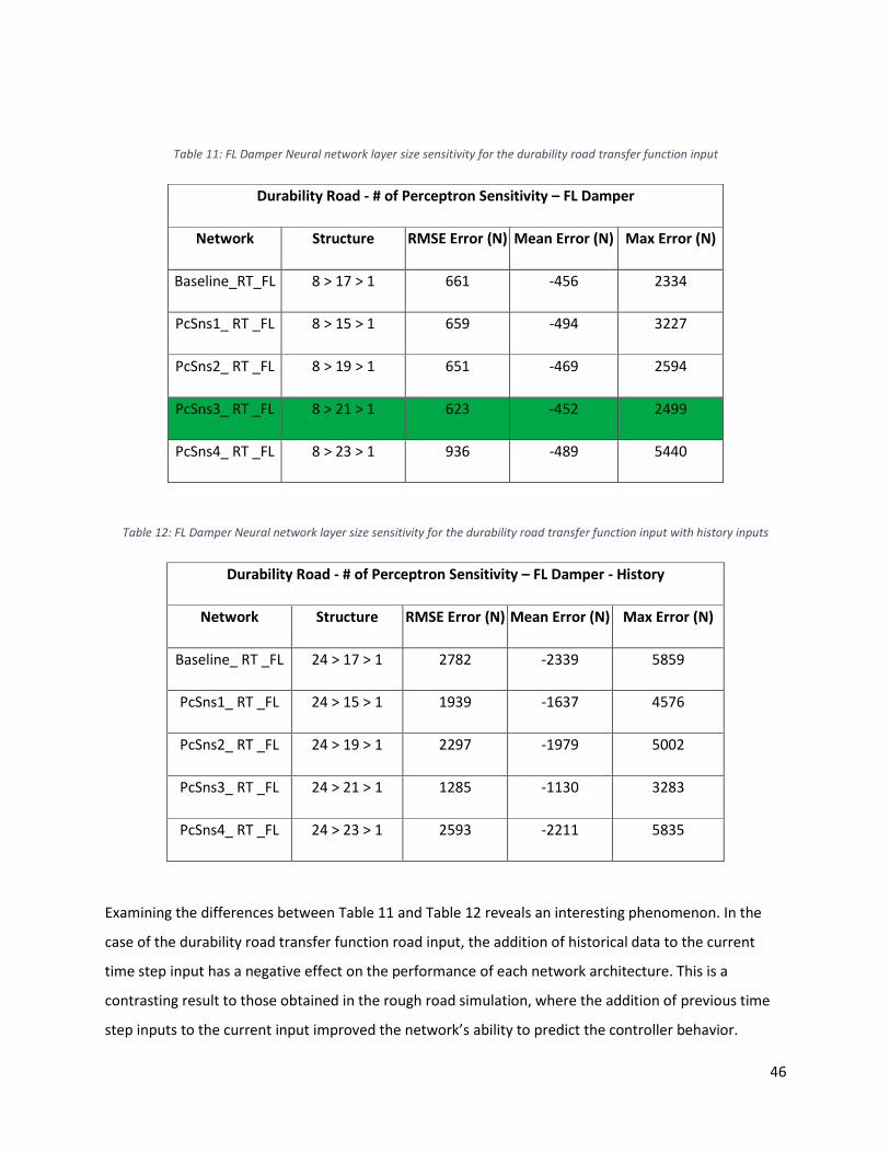
46

Table 11: FL Damper Neural network layer size sensitivity for the durability road transfer function input

Durability Road - # of Perceptron Sensitivity – FL Damper

Network Structure RMSE Error (N) Mean Error (N) Max Error (N)

Baseline_RT_FL 8 > 17 > 1 661 -456 2334

PcSns1_ RT _FL 8 > 15 > 1 659 -494 3227

PcSns2_ RT _FL 8 > 19 > 1 651 -469 2594

PcSns3_ RT _FL 8 > 21 > 1 623 -452 2499

PcSns4_ RT _FL 8 > 23 > 1 936 -489 5440

Table 12: FL Damper Neural network layer size sensitivity for the durability road transfer function input with history inputs

Durability Road - # of Perceptron Sensitivity – FL Damper - History

Network Structure RMSE Error (N) Mean Error (N) Max Error (N)

Baseline_ RT _FL 24 > 17 > 1 2782 -2339 5859

PcSns1_ RT _FL 24 > 15 > 1 1939 -1637 4576

PcSns2_ RT _FL 24 > 19 > 1 2297 -1979 5002

PcSns3_ RT _FL 24 > 21 > 1 1285 -1130 3283

PcSns4_ RT _FL 24 > 23 > 1 2593 -2211 5835

Examining the differences between Table 11 and Table 12 reveals an interesting phenomenon. In the

case of the durability road transfer function road input, the addition of historical data to the current

time step input has a negative effect on the performance of each network architecture. This is a

contrasting result to those obtained in the rough road simulation, where the addition of previous time

step inputs to the current input improved the network’s ability to predict the controller behavior.

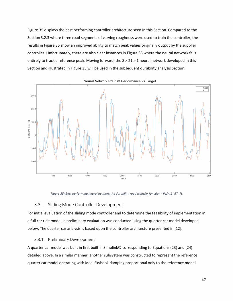
47

Figure 35 displays the best performing controller architecture seen in this Section. Compared to the

Section 3.2.3 where three road segments of varying roughness were used to train the controller, the

results in Figure 35 show an improved ability to match peak values originally output by the supplier

controller. Unfortunately, there are also clear instances in Figure 35 where the neural network fails

entirely to track a reference peak. Moving forward, the 8 > 21 > 1 neural network developed in this

Section and illustrated in Figure 35 will be used in the subsequent durability analysis Section.

Figure 35: Best performing neural network the durability road transfer function - PcSns3_RT_FL

3.3. Sliding Mode Controller Development

For initial evaluation of the sliding mode controller and to determine the feasibility of implementation in

a full car ride model, a preliminary evaluation was conducted using the quarter car model developed

below. The quarter car analysis is based upon the controller architecture presented in [12].

3.3.1. Preliminary Development

A quarter car model was built in first built in Simulink© corresponding to Equations (23) and (24)

detailed above. In a similar manner, another subsystem was constructed to represent the reference

quarter car model operating with ideal Skyhook damping proportional only to the reference model

Neural Network PcSns3 Performance vs Target

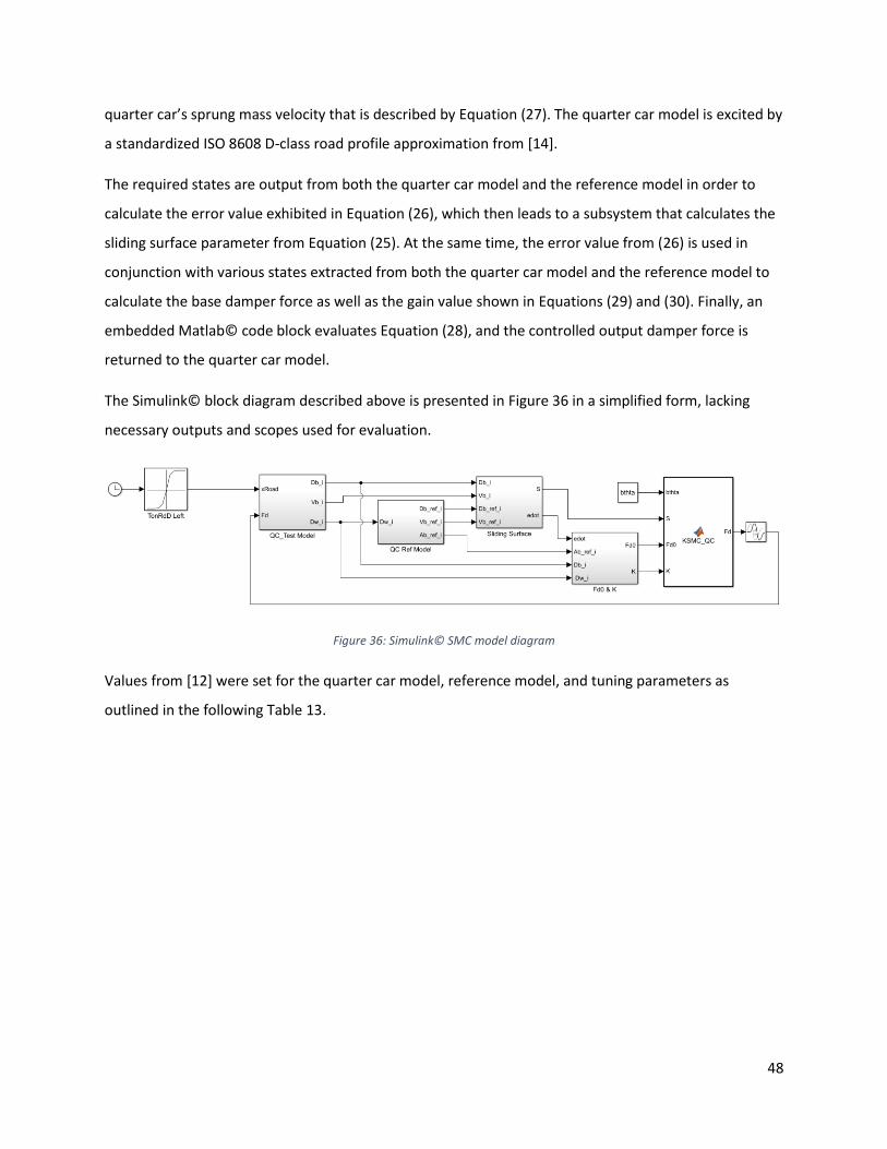
48

quarter car’s sprung mass velocity that is described by Equation (27). The quarter car model is excited by

a standardized ISO 8608 D-class road profile approximation from [14].

The required states are output from both the quarter car model and the reference model in order to

calculate the error value exhibited in Equation (26), which then leads to a subsystem that calculates the

sliding surface parameter from Equation (25). At the same time, the error value from (26) is used in

conjunction with various states extracted from both the quarter car model and the reference model to

calculate the base damper force as well as the gain value shown in Equations (29) and (30). Finally, an

embedded Matlab© code block evaluates Equation (28), and the controlled output damper force is

returned to the quarter car model.

The Simulink© block diagram described above is presented in Figure 36 in a simplified form, lacking

necessary outputs and scopes used for evaluation.

Figure 36: Simulink© SMC model diagram

Values from [12] were set for the quarter car model, reference model, and tuning parameters as

outlined in the following Table 13.

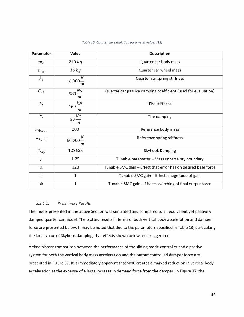
49

Table 13: Quarter car simulation parameter values [12]

Parameter Value Description

𝑚𝑏 240 𝑘𝑔 Quarter car body mass

𝑚𝑤 36 𝑘𝑔 Quarter car wheel mass

𝑘𝑠 16,000𝑁

𝑚

Quarter car spring stiffness

𝐶𝑑𝑃 980

𝑁𝑠

𝑚

Quarter car passive damping coefficient (used for evaluation)

𝑘𝑡 160𝑘𝑁

𝑚

Tire stiffness

𝐶𝑡 50𝑁𝑠

𝑚

Tire damping

𝑚𝑏𝑅𝐸𝐹 200 Reference body mass

𝑘𝑠𝑅𝐸𝐹 50,000

𝑁

𝑚

Reference spring stiffness

𝐶𝑆𝑘𝑦 128625 Skyhook Damping

𝜇 1.25 Tunable parameter – Mass uncertainty boundary

𝜆 120 Tunable SMC gain – Effect that error has on desired base force

𝜖 1 Tunable SMC gain – Effects magnitude of gain

Φ 1 Tunable SMC gain – Effects switching of final output force

3.3.1.1. Preliminary Results

The model presented in the above Section was simulated and compared to an equivalent yet passively

damped quarter car model. The plotted results in terms of both vertical body acceleration and damper

force are presented below. It may be noted that due to the parameters specified in Table 13, particularly

the large value of Skyhook damping, that effects shown below are exaggerated.

A time history comparison between the performance of the sliding mode controller and a passive

system for both the vertical body mass acceleration and the output controlled damper force are

presented in Figure 37. It is immediately apparent that SMC creates a marked reduction in vertical body

acceleration at the expense of a large increase in demand force from the damper. In Figure 37, the

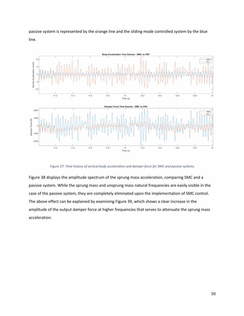
50

passive system is represented by the orange line and the sliding mode controlled system by the blue

line.

Figure 37: Time history of vertical body acceleration and damper force for SMC and passive systems

Figure 38 displays the amplitude spectrum of the sprung mass acceleration, comparing SMC and a

passive system. While the sprung mass and unsprung mass natural frequencies are easily visible in the

case of the passive system, they are completely eliminated upon the implementation of SMC control.

The above effect can be explained by examining Figure 39, which shows a clear increase in the

amplitude of the output damper force at higher frequencies that serves to attenuate the sprung mass

acceleration.

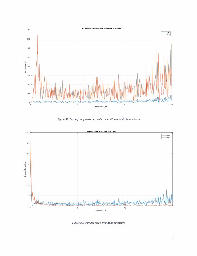
51

Figure 38: Sprung body mass vertical acceleration amplitude spectrum

Figure 39: Damper force amplitude spectrum

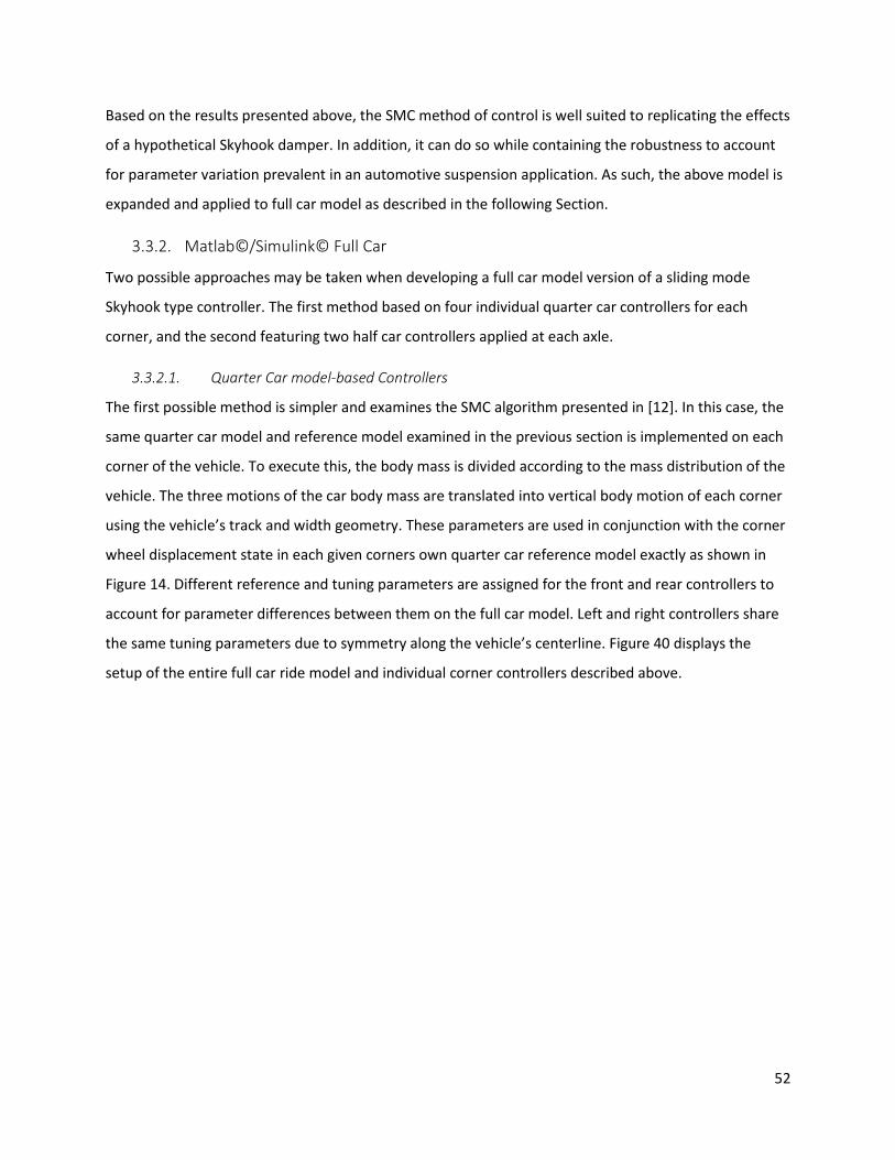
52

Based on the results presented above, the SMC method of control is well suited to replicating the effects

of a hypothetical Skyhook damper. In addition, it can do so while containing the robustness to account

for parameter variation prevalent in an automotive suspension application. As such, the above model is

expanded and applied to full car model as described in the following Section.

3.3.2. Matlab©/Simulink© Full Car

Two possible approaches may be taken when developing a full car model version of a sliding mode

Skyhook type controller. The first method based on four individual quarter car controllers for each

corner, and the second featuring two half car controllers applied at each axle.

3.3.2.1. Quarter Car model-based Controllers

The first possible method is simpler and examines the SMC algorithm presented in [12]. In this case, the

same quarter car model and reference model examined in the previous section is implemented on each

corner of the vehicle. To execute this, the body mass is divided according to the mass distribution of the

vehicle. The three motions of the car body mass are translated into vertical body motion of each corner

using the vehicle’s track and width geometry. These parameters are used in conjunction with the corner

wheel displacement state in each given corners own quarter car reference model exactly as shown in

Figure 14. Different reference and tuning parameters are assigned for the front and rear controllers to

account for parameter differences between them on the full car model. Left and right controllers share

the same tuning parameters due to symmetry along the vehicle’s centerline. Figure 40 displays the

setup of the entire full car ride model and individual corner controllers described above.

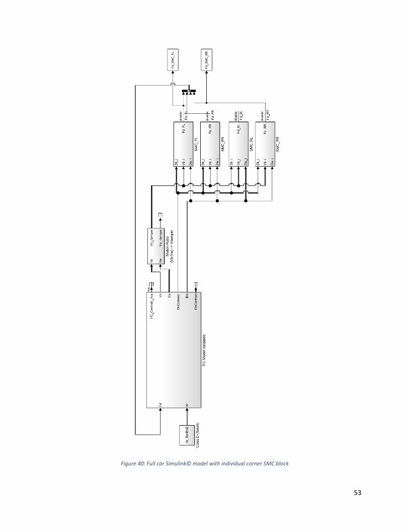
53

Figure 40: Full car Simulink© model with individual corner SMC block

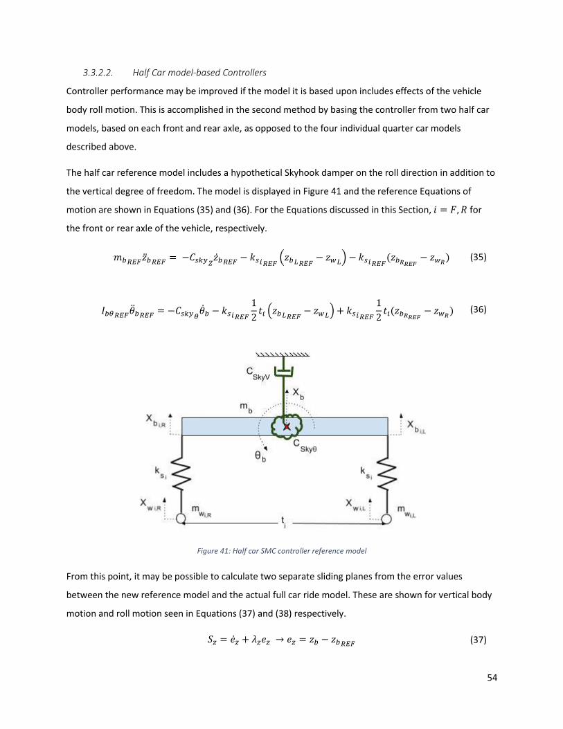
54

3.3.2.2. Half Car model-based Controllers

Controller performance may be improved if the model it is based upon includes effects of the vehicle

body roll motion. This is accomplished in the second method by basing the controller from two half car

models, based on each front and rear axle, as opposed to the four individual quarter car models

described above.

The half car reference model includes a hypothetical Skyhook damper on the roll direction in addition to

the vertical degree of freedom. The model is displayed in Figure 41 and the reference Equations of

motion are shown in Equations (35) and (36). For the Equations discussed in this Section, 𝑖 = 𝐹, 𝑅 for

the front or rear axle of the vehicle, respectively.

𝑚𝑏𝑅𝐸𝐹�̈�𝑏𝑅𝐸𝐹 = −𝐶𝑠𝑘𝑦𝑍�̇�𝑏𝑅𝐸𝐹 − 𝑘𝑠𝑖𝑅𝐸𝐹(𝑧𝑏𝐿𝑅𝐸𝐹

− 𝑧𝑤𝐿) − 𝑘𝑠𝑖𝑅𝐸𝐹(𝑧𝑏𝑅𝑅𝐸𝐹

− 𝑧𝑤𝑅) (35)

𝐼𝑏𝜃𝑅𝐸𝐹�̈�𝑏𝑅𝐸𝐹 = −𝐶𝑠𝑘𝑦𝜃�̇�𝑏 − 𝑘𝑠𝑖𝑅𝐸𝐹

1

2𝑡𝑖 (𝑧𝑏𝐿𝑅𝐸𝐹

− 𝑧𝑤𝐿) + 𝑘𝑠𝑖𝑅𝐸𝐹

1

2𝑡𝑖(𝑧𝑏𝑅𝑅𝐸𝐹

− 𝑧𝑤𝑅) (36)

Figure 41: Half car SMC controller reference model

From this point, it may be possible to calculate two separate sliding planes from the error values

between the new reference model and the actual full car ride model. These are shown for vertical body

motion and roll motion seen in Equations (37) and (38) respectively.

𝑆𝑧 = �̇�𝑧 + 𝜆𝑧𝑒𝑧 → 𝑒𝑧 = 𝑧𝑏 − 𝑧𝑏𝑅𝐸𝐹 (37)

55

𝑆𝜃 = �̇�𝜃 + 𝜆𝜃𝑒𝜃 → 𝑒𝜃 = 𝜃𝑏 − 𝜃𝑏𝑅𝐸𝐹 (38)

Moving forward, methods described in [13] used on a quarter car sliding mode controller are

extrapolated to the half car model. The resulting set of equations describing the ideal control vertical

damping force and roll torque are described in Equations (39) and (40).

𝐹𝑑0 = 𝐹𝑑0𝐿 + 𝐹𝑑0𝑅 = −𝑘𝑠𝑖(𝑧𝑏𝐿 − 𝑧𝑤𝐿) − 𝑘𝑠𝑖(𝑧𝑏𝑅 − 𝑧𝑤𝑅) − 𝑚𝑏0�̈�𝑏𝑅𝐸𝐹 +𝑚𝑏0𝜆𝑧�̇�𝑧 (39)

𝑇𝑑0 = −𝐹𝑑0𝐿1

2𝑡𝑖 + 𝐹𝑑0𝑅𝑙𝑅

1

2𝑡𝑖

= −𝑘𝑠𝑖1

2𝑡𝑖(𝑧𝑏𝐿 − 𝑧𝑤𝐿) + 𝑘𝑠𝑖

1

2𝑡𝑖(𝑧𝑏𝑅 − 𝑧𝑤𝑅) − 𝐼𝑏𝜃0�̈�𝑏𝑅𝐸𝐹 + 𝐼𝑏𝜃0𝜆𝜃�̇�𝜃

(40)

Similarly to the above, the gain parameter that aids in smooth damper output transitions [13] is

calculated below for vertical and roll modes as follows in Equations (41) and (42).

𝐾𝑧 = (𝜇𝑧 − 1) (|𝐹𝑑0| + 𝑘𝑠𝑖(|𝑧𝑏𝐹| + |𝑧𝑤𝐹|) + 𝑘𝑠𝑖(|𝑧𝑏𝑅| + |𝑧𝑤𝑅|)) + 𝑚𝑏0𝜇𝑧𝜖𝑧 (41)

𝐾𝜃 = (𝜇𝜃 − 1)(|𝑇𝑑0| + 𝑘𝑠𝑖1

2𝑡𝑖(|𝑧𝑏𝐹| + |𝑧𝑤𝐹|) + 𝑘𝑠𝑖

1

2𝑡𝑖(|𝑧𝑏𝑅| + |𝑧𝑤𝑅|)) + 𝐼𝑏𝜃0𝜇𝜃𝜖𝜃 (42)

Control force and torque are calculated based on the condition of the sliding surfaces relative to their

respective tuning parameters Φ𝑧 or Φθ.

𝐹𝑑𝑐 = 𝐹𝑑0 + {𝐾𝑧𝑣𝑎𝑙(𝑆𝑧) → |𝑆𝑧| ≤ Φz

𝐾𝑧𝑠𝑔𝑛(𝑆𝑧) → |𝑆𝑧| > Φz} (43)

𝑇𝑑𝑐 = 𝑇𝑑0 + {𝐾𝜃𝑣𝑎𝑙(𝑆𝜃) → |𝑆𝜃| ≤ Φ𝜃

𝐾𝜃𝑠𝑔𝑛(𝑆𝜃) → |𝑆𝜃| > Φ𝜃} (44)

56

Equations (43) and (44) calculate the desired damper force and torque that would need to be applied at

the center of the half car wheelbase. To establish the desired force that must be applied at each corner

in order to recreate 𝐹𝑑𝑐 and 𝑇𝑑𝑐, the linear system in Equation (45) based on the vehicle’s geometry

must be solved.

[1 11

2𝑡𝑖 −

1

2𝑡𝑖] [𝐹𝑑𝐹𝐹𝑑𝑅

] = [𝐹𝑑𝑐𝑇𝑑𝑐

] (45)

Finally, Figure 42 shows the overall Simulink© construction of the implementation of sliding mode

control with two half car based controllers. Despite there being two separate controllers, each is fed

with the same roll and vertical sprung body motion seen in the reference full car model. The difference

between front and rear controllers is that each controller only receives its respective front or rear wheel

corner displacement.

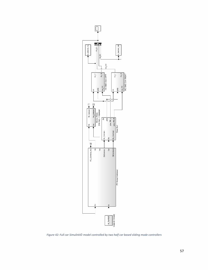
57

Figure 42: Full car Simulink© model controlled by two half car based sliding mode controllers

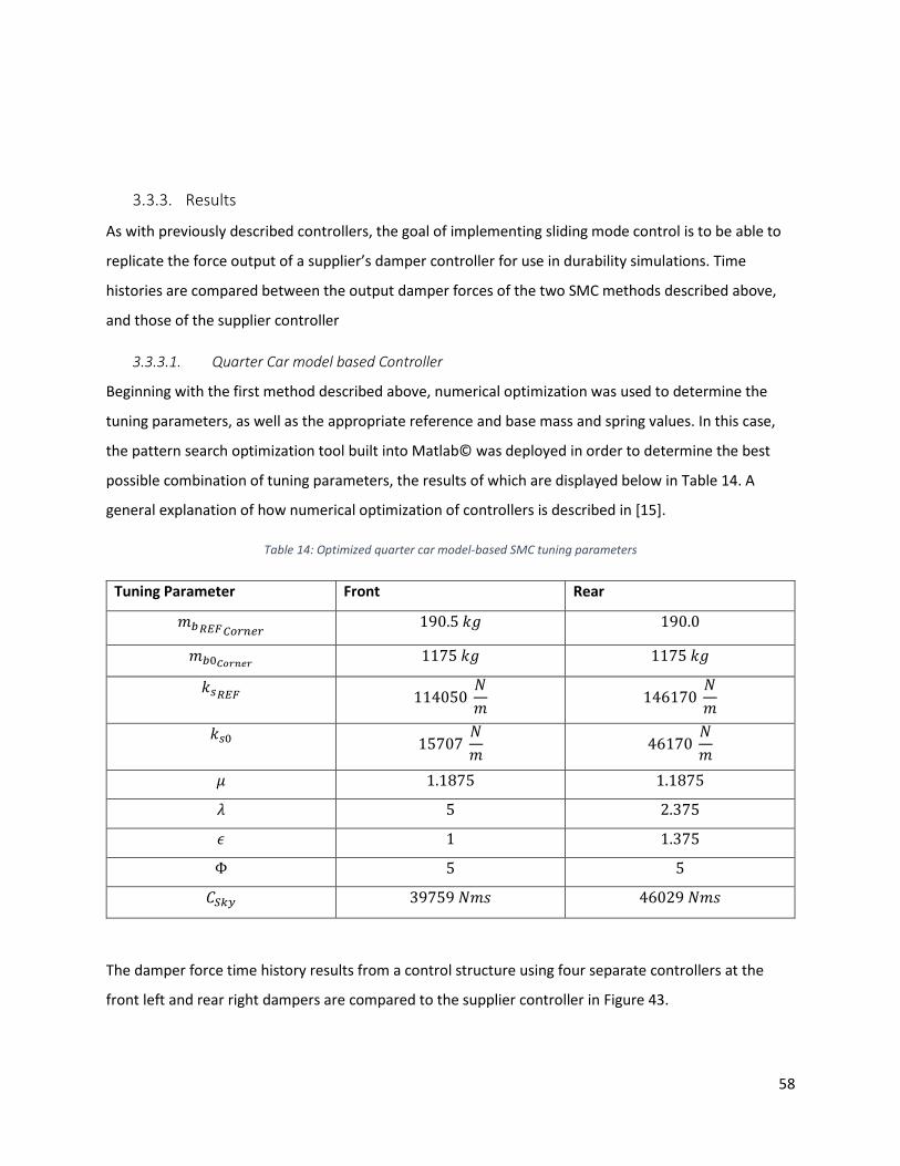
58

3.3.3. Results

As with previously described controllers, the goal of implementing sliding mode control is to be able to

replicate the force output of a supplier’s damper controller for use in durability simulations. Time

histories are compared between the output damper forces of the two SMC methods described above,

and those of the supplier controller

3.3.3.1. Quarter Car model based Controller

Beginning with the first method described above, numerical optimization was used to determine the

tuning parameters, as well as the appropriate reference and base mass and spring values. In this case,

the pattern search optimization tool built into Matlab© was deployed in order to determine the best

possible combination of tuning parameters, the results of which are displayed below in Table 14. A

general explanation of how numerical optimization of controllers is described in [15].

Table 14: Optimized quarter car model-based SMC tuning parameters

Tuning Parameter Front Rear

𝑚𝑏𝑅𝐸𝐹𝐶𝑜𝑟𝑛𝑒𝑟 190.5 𝑘𝑔 190.0

𝑚𝑏0𝐶𝑜𝑟𝑛𝑒𝑟 1175 𝑘𝑔 1175 𝑘𝑔

𝑘𝑠𝑅𝐸𝐹 114050

𝑁

𝑚 146170

𝑁

𝑚

𝑘𝑠0 15707

𝑁

𝑚 46170

𝑁

𝑚

𝜇 1.1875 1.1875

𝜆 5 2.375

𝜖 1 1.375

Φ 5 5

𝐶𝑆𝑘𝑦 39759 𝑁𝑚𝑠 46029 𝑁𝑚𝑠

The damper force time history results from a control structure using four separate controllers at the

front left and rear right dampers are compared to the supplier controller in Figure 43.

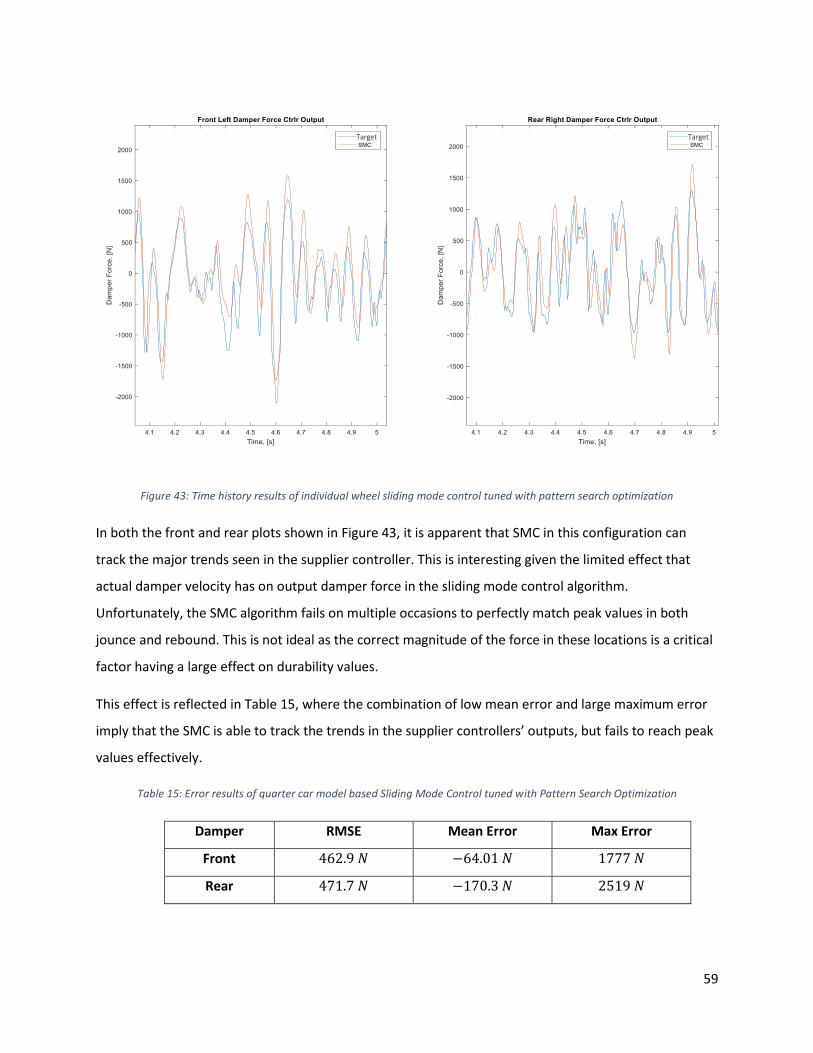
59

Figure 43: Time history results of individual wheel sliding mode control tuned with pattern search optimization

In both the front and rear plots shown in Figure 43, it is apparent that SMC in this configuration can

track the major trends seen in the supplier controller. This is interesting given the limited effect that

actual damper velocity has on output damper force in the sliding mode control algorithm.

Unfortunately, the SMC algorithm fails on multiple occasions to perfectly match peak values in both

jounce and rebound. This is not ideal as the correct magnitude of the force in these locations is a critical

factor having a large effect on durability values.

This effect is reflected in Table 15, where the combination of low mean error and large maximum error

imply that the SMC is able to track the trends in the supplier controllers’ outputs, but fails to reach peak

values effectively.

Table 15: Error results of quarter car model based Sliding Mode Control tuned with Pattern Search Optimization

Damper RMSE Mean Error Max Error

Front 462.9 𝑁 −64.01 𝑁 1777 𝑁

Rear 471.7 𝑁 −170.3 𝑁 2519 𝑁

Target Target

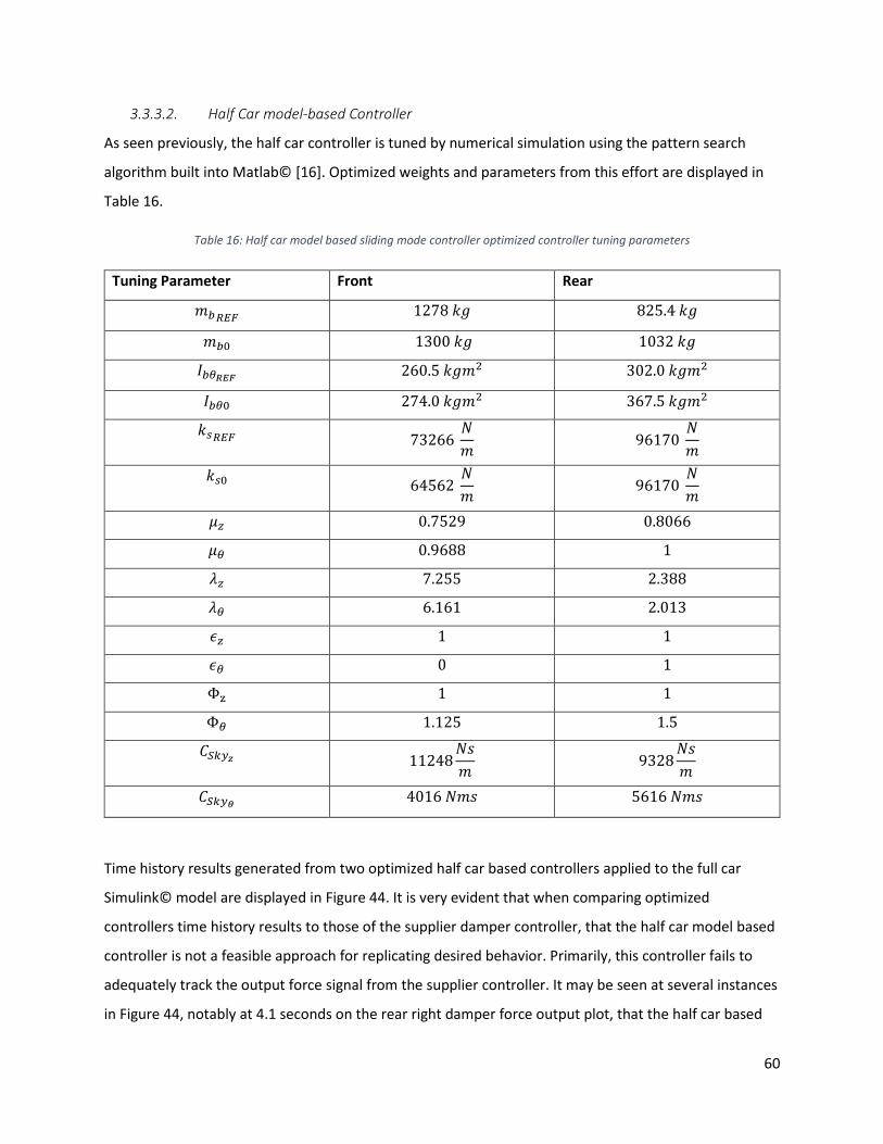
60

3.3.3.2. Half Car model-based Controller

As seen previously, the half car controller is tuned by numerical simulation using the pattern search

algorithm built into Matlab© [16]. Optimized weights and parameters from this effort are displayed in

Table 16.

Table 16: Half car model based sliding mode controller optimized controller tuning parameters

Tuning Parameter Front Rear

𝑚𝑏𝑅𝐸𝐹 1278 𝑘𝑔 825.4 𝑘𝑔

𝑚𝑏0 1300 𝑘𝑔 1032 𝑘𝑔

𝐼𝑏𝜃𝑅𝐸𝐹 260.5 𝑘𝑔𝑚2 302.0 𝑘𝑔𝑚2

𝐼𝑏𝜃0 274.0 𝑘𝑔𝑚2 367.5 𝑘𝑔𝑚2

𝑘𝑠𝑅𝐸𝐹 73266

𝑁

𝑚 96170

𝑁

𝑚

𝑘𝑠0 64562

𝑁

𝑚 96170

𝑁

𝑚

𝜇𝑧 0.7529 0.8066

𝜇𝜃 0.9688 1

𝜆𝑧 7.255 2.388

𝜆𝜃 6.161 2.013

𝜖𝑧 1 1

𝜖𝜃 0 1

Φz 1 1

Φ𝜃 1.125 1.5

𝐶𝑆𝑘𝑦𝑧 11248

𝑁𝑠

𝑚 9328

𝑁𝑠

𝑚

𝐶𝑆𝑘𝑦𝜃 4016 𝑁𝑚𝑠 5616 𝑁𝑚𝑠

Time history results generated from two optimized half car based controllers applied to the full car

Simulink© model are displayed in Figure 44. It is very evident that when comparing optimized

controllers time history results to those of the supplier damper controller, that the half car model based

controller is not a feasible approach for replicating desired behavior. Primarily, this controller fails to

adequately track the output force signal from the supplier controller. It may be seen at several instances

in Figure 44, notably at 4.1 seconds on the rear right damper force output plot, that the half car based

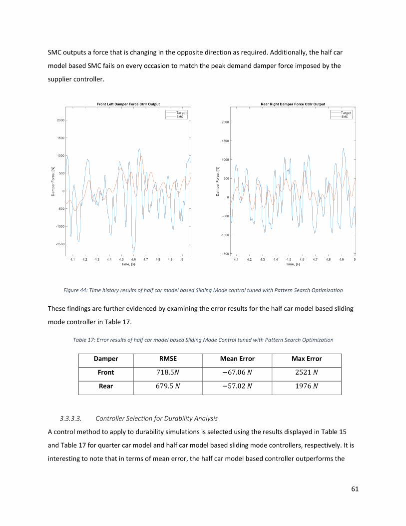
61

SMC outputs a force that is changing in the opposite direction as required. Additionally, the half car

model based SMC fails on every occasion to match the peak demand damper force imposed by the

supplier controller.

Figure 44: Time history results of half car model based Sliding Mode control tuned with Pattern Search Optimization

These findings are further evidenced by examining the error results for the half car model based sliding

mode controller in Table 17.

Table 17: Error results of half car model based Sliding Mode Control tuned with Pattern Search Optimization

Damper RMSE Mean Error Max Error

Front 718.5𝑁 −67.06 𝑁 2521 𝑁

Rear 679.5 𝑁 −57.02 𝑁 1976 𝑁

3.3.3.3. Controller Selection for Durability Analysis

A control method to apply to durability simulations is selected using the results displayed in Table 15

and Table 17 for quarter car model and half car model based sliding mode controllers, respectively. It is

interesting to note that in terms of mean error, the half car model based controller outperforms the

Target Target

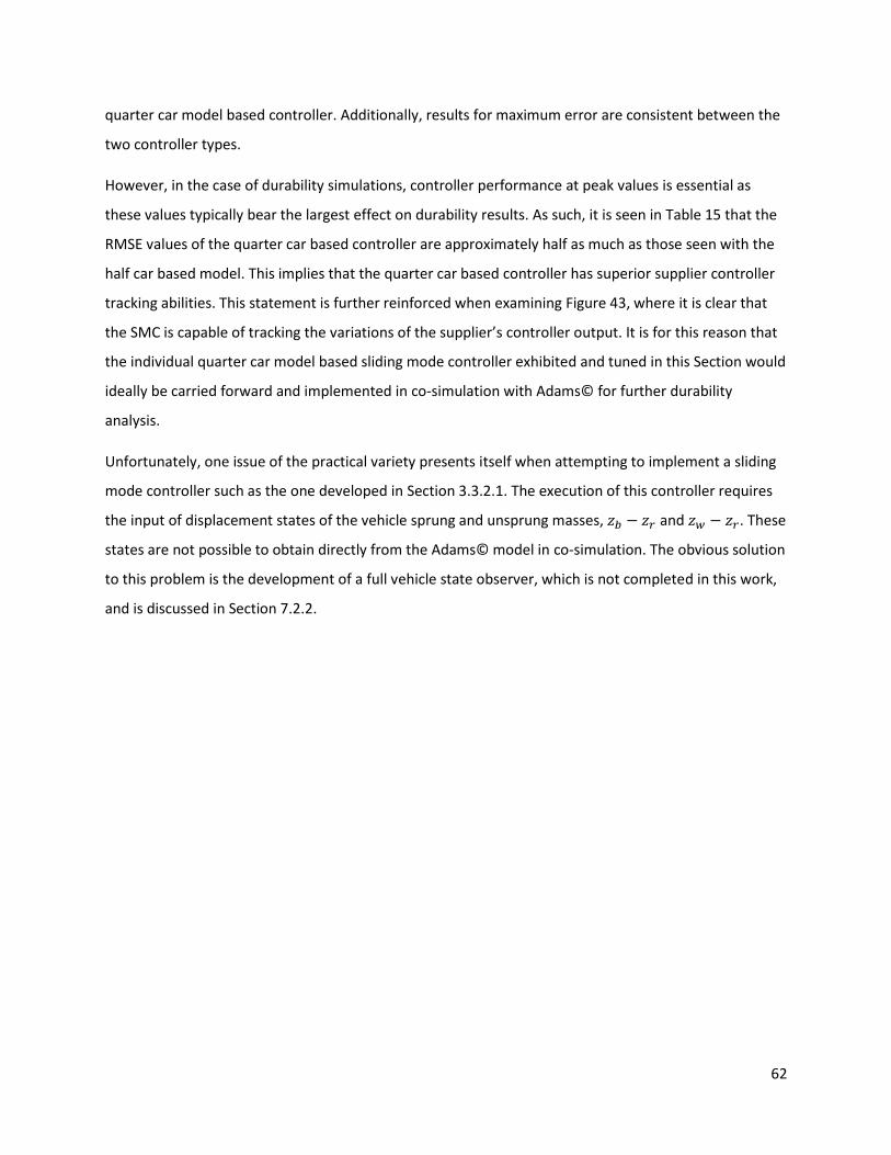
62

quarter car model based controller. Additionally, results for maximum error are consistent between the

two controller types.

However, in the case of durability simulations, controller performance at peak values is essential as

these values typically bear the largest effect on durability results. As such, it is seen in Table 15 that the

RMSE values of the quarter car based controller are approximately half as much as those seen with the

half car based model. This implies that the quarter car based controller has superior supplier controller

tracking abilities. This statement is further reinforced when examining Figure 43, where it is clear that

the SMC is capable of tracking the variations of the supplier’s controller output. It is for this reason that

the individual quarter car model based sliding mode controller exhibited and tuned in this Section would

ideally be carried forward and implemented in co-simulation with Adams© for further durability

analysis.

Unfortunately, one issue of the practical variety presents itself when attempting to implement a sliding

mode controller such as the one developed in Section 3.3.2.1. The execution of this controller requires

the input of displacement states of the vehicle sprung and unsprung masses, 𝑧𝑏 − 𝑧𝑟 and 𝑧𝑤 − 𝑧𝑟. These

states are not possible to obtain directly from the Adams© model in co-simulation. The obvious solution

to this problem is the development of a full vehicle state observer, which is not completed in this work,

and is discussed in Section 7.2.2.

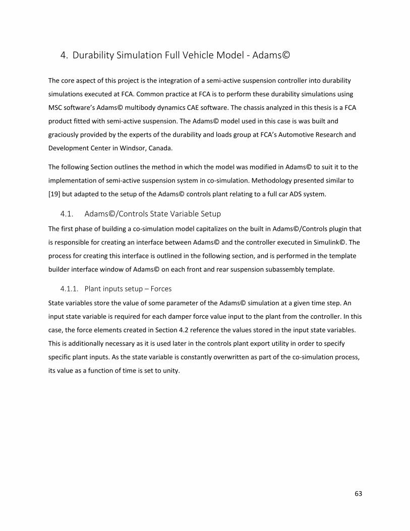
63

4. Durability Simulation Full Vehicle Model - Adams©

The core aspect of this project is the integration of a semi-active suspension controller into durability

simulations executed at FCA. Common practice at FCA is to perform these durability simulations using

MSC software’s Adams© multibody dynamics CAE software. The chassis analyzed in this thesis is a FCA

product fitted with semi-active suspension. The Adams© model used in this case is was built and

graciously provided by the experts of the durability and loads group at FCA’s Automotive Research and

Development Center in Windsor, Canada.

The following Section outlines the method in which the model was modified in Adams© to suit it to the

implementation of semi-active suspension system in co-simulation. Methodology presented similar to

[19] but adapted to the setup of the Adams© controls plant relating to a full car ADS system.

4.1. Adams©/Controls State Variable Setup

The first phase of building a co-simulation model capitalizes on the built in Adams©/Controls plugin that

is responsible for creating an interface between Adams© and the controller executed in Simulink©. The

process for creating this interface is outlined in the following section, and is performed in the template

builder interface window of Adams© on each front and rear suspension subassembly template.

4.1.1. Plant inputs setup – Forces

State variables store the value of some parameter of the Adams© simulation at a given time step. An

input state variable is required for each damper force value input to the plant from the controller. In this

case, the force elements created in Section 4.2 reference the values stored in the input state variables.

This is additionally necessary as it is used later in the controls plant export utility in order to specify

specific plant inputs. As the state variable is constantly overwritten as part of the co-simulation process,

its value as a function of time is set to unity.

64

Figure 45: Adams© State Variable setup window for damper force plant input

4.1.2. Outputs setup – Damper velocity, body acceleration, etc.

Output state variables are created to measure the values of plant states required to be exported to the

Simulink© controller. These are declared using the Adams© function builder that calculates either the

desired acceleration, velocity, or displacement between the appropriate markers. The example shown is

the creation of the damper velocity state variable, as it is required by virtually any virtual damper

controller. Additional outputs for body acceleration and body – wheel relative displacement are

declared similarly.

As shown in Figure 46, the damper velocity output state variable is declared using the built-in Adams©

relative velocity function referencing the velocity between the i and j damper markers. This results in a

damper velocity output along the axis of the damper, accounting for the installation orientation of the

damper, and is setup as follows:

Figure 46: Adams© State Variable setup window for plant outputs

It must be noted that the above methodology of damper velocity measurement should work in all cases,

instability in the velocity channels transferred to Simulink© existed for the rear subsystem of the model

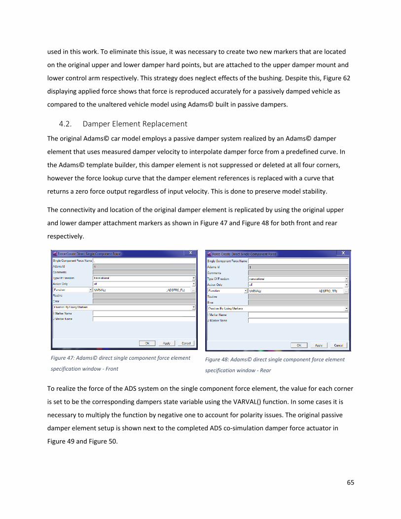
65

used in this work. To eliminate this issue, it was necessary to create two new markers that are located

on the original upper and lower damper hard points, but are attached to the upper damper mount and

lower control arm respectively. This strategy does neglect effects of the bushing. Despite this, Figure 62

displaying applied force shows that force is reproduced accurately for a passively damped vehicle as

compared to the unaltered vehicle model using Adams© built in passive dampers.

4.2. Damper Element Replacement

The original Adams© car model employs a passive damper system realized by an Adams© damper

element that uses measured damper velocity to interpolate damper force from a predefined curve. In

the Adams© template builder, this damper element is not suppressed or deleted at all four corners,

however the force lookup curve that the damper element references is replaced with a curve that

returns a zero force output regardless of input velocity. This is done to preserve model stability.

The connectivity and location of the original damper element is replicated by using the original upper

and lower damper attachment markers as shown in Figure 47 and Figure 48 for both front and rear

respectively.

Figure 47: Adams© direct single component force element

specification window - Front

Figure 48: Adams© direct single component force element

specification window - Rear

To realize the force of the ADS system on the single component force element, the value for each corner

is set to be the corresponding dampers state variable using the VARVAL() function. In some cases it is

necessary to multiply the function by negative one to account for polarity issues. The original passive

damper element setup is shown next to the completed ADS co-simulation damper force actuator in

Figure 49 and Figure 50.

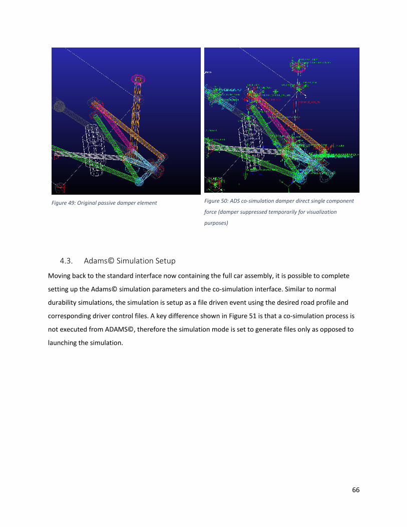
66

Figure 49: Original passive damper element

Figure 50: ADS co-simulation damper direct single component

force (damper suppressed temporarily for visualization

purposes)

4.3. Adams© Simulation Setup

Moving back to the standard interface now containing the full car assembly, it is possible to complete

setting up the Adams© simulation parameters and the co-simulation interface. Similar to normal

durability simulations, the simulation is setup as a file driven event using the desired road profile and

corresponding driver control files. A key difference shown in Figure 51 is that a co-simulation process is

not executed from ADAMS©, therefore the simulation mode is set to generate files only as opposed to

launching the simulation.

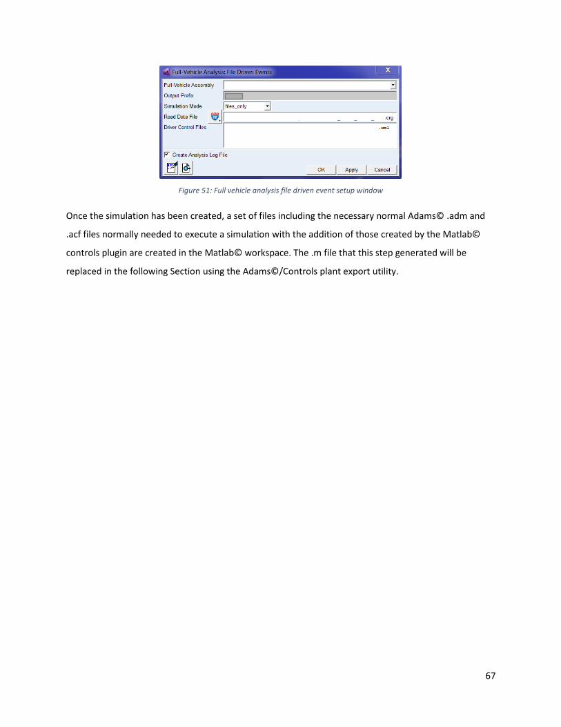
67

Figure 51: Full vehicle analysis file driven event setup window

Once the simulation has been created, a set of files including the necessary normal Adams© .adm and

.acf files normally needed to execute a simulation with the addition of those created by the Matlab©

controls plugin are created in the Matlab© workspace. The .m file that this step generated will be

replaced in the following Section using the Adams©/Controls plant export utility.

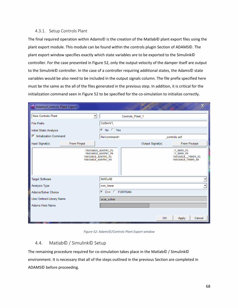
68

4.3.1. Setup Controls Plant

The final required operation within Adams© is the creation of the Matlab© plant export files using the

plant export module. This module can be found within the controls plugin Section of ADAMS©. The

plant export window specifies exactly which state variables are to be exported to the Simulink©

controller. For the case presented in Figure 52, only the output velocity of the damper itself are output

to the Simulink© controller. In the case of a controller requiring additional states, the Adams© state

variables would be also need to be included in the output signals column. The file prefix specified here

must be the same as the all of the files generated in the previous step. In addition, it is critical for the

initialization command seen in Figure 52 to be specified for the co-simulation to initialize correctly.

Figure 52: Adams©/Controls Plant Export window

4.4. Matlab© / Simulink© Setup

The remaining procedure required for co-simulation takes place in the Matlab© / Simulink©

environment. It is necessary that all of the steps outlined in the previous Section are completed in

ADAMS© before proceeding.

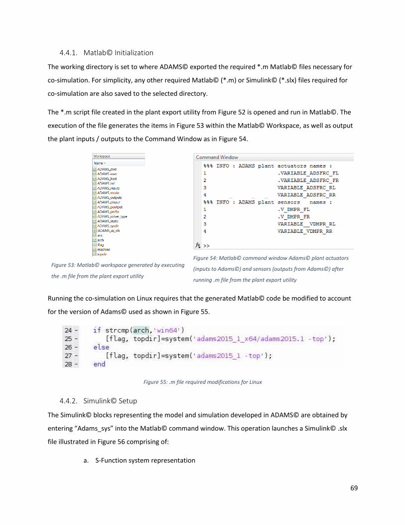
69

4.4.1. Matlab© Initialization

The working directory is set to where ADAMS© exported the required *.m Matlab© files necessary for

co-simulation. For simplicity, any other required Matlab© (*.m) or Simulink© (*.slx) files required for

co-simulation are also saved to the selected directory.

The *.m script file created in the plant export utility from Figure 52 is opened and run in Matlab©. The

execution of the file generates the items in Figure 53 within the Matlab© Workspace, as well as output

the plant inputs / outputs to the Command Window as in Figure 54.

Figure 53: Matlab© workspace generated by executing

the .m file from the plant export utility

Figure 54: Matlab© command window Adams© plant actuators

(inputs to Adams©) and sensors (outputs from Adams©) after

running .m file from the plant export utility

Running the co-simulation on Linux requires that the generated Matlab© code be modified to account

for the version of Adams© used as shown in Figure 55.

Figure 55: .m file required modifications for Linux

4.4.2. Simulink© Setup

The Simulink© blocks representing the model and simulation developed in ADAMS© are obtained by

entering “Adams_sys” into the Matlab© command window. This operation launches a Simulink© .slx

file illustrated in Figure 56 comprising of:

a. S-Function system representation

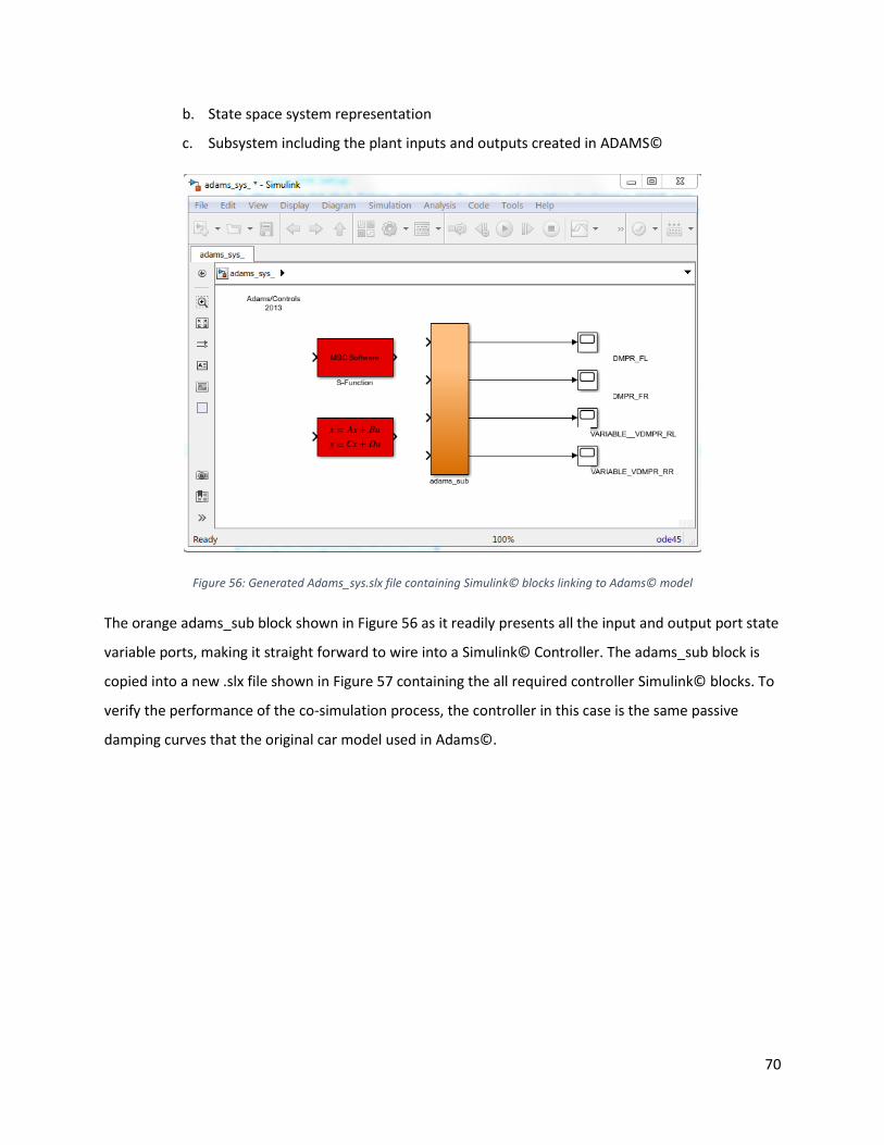
70

b. State space system representation

c. Subsystem including the plant inputs and outputs created in ADAMS©

Figure 56: Generated Adams_sys.slx file containing Simulink© blocks linking to Adams© model

The orange adams_sub block shown in Figure 56 as it readily presents all the input and output port state

variable ports, making it straight forward to wire into a Simulink© Controller. The adams_sub block is

copied into a new .slx file shown in Figure 57 containing the all required controller Simulink© blocks. To

verify the performance of the co-simulation process, the controller in this case is the same passive

damping curves that the original car model used in Adams©.

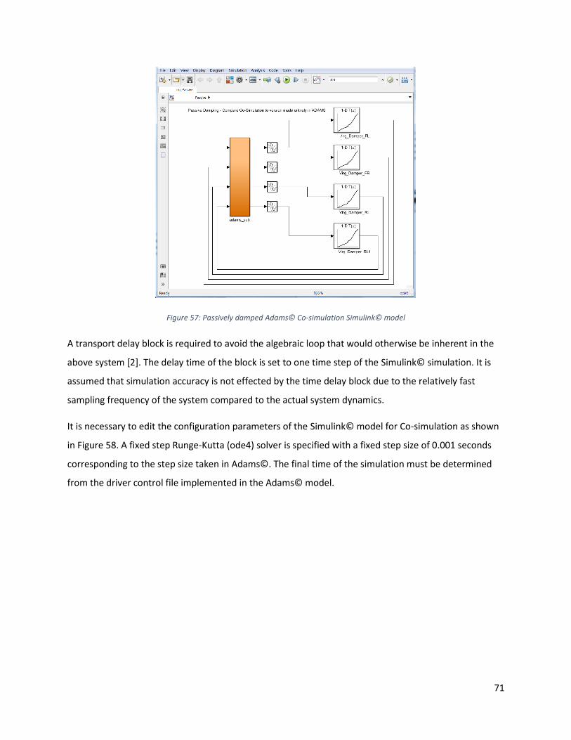
71

Figure 57: Passively damped Adams© Co-simulation Simulink© model

A transport delay block is required to avoid the algebraic loop that would otherwise be inherent in the

above system [2]. The delay time of the block is set to one time step of the Simulink© simulation. It is

assumed that simulation accuracy is not effected by the time delay block due to the relatively fast

sampling frequency of the system compared to the actual system dynamics.

It is necessary to edit the configuration parameters of the Simulink© model for Co-simulation as shown

in Figure 58. A fixed step Runge-Kutta (ode4) solver is specified with a fixed step size of 0.001 seconds

corresponding to the step size taken in Adams©. The final time of the simulation must be determined

from the driver control file implemented in the Adams© model.

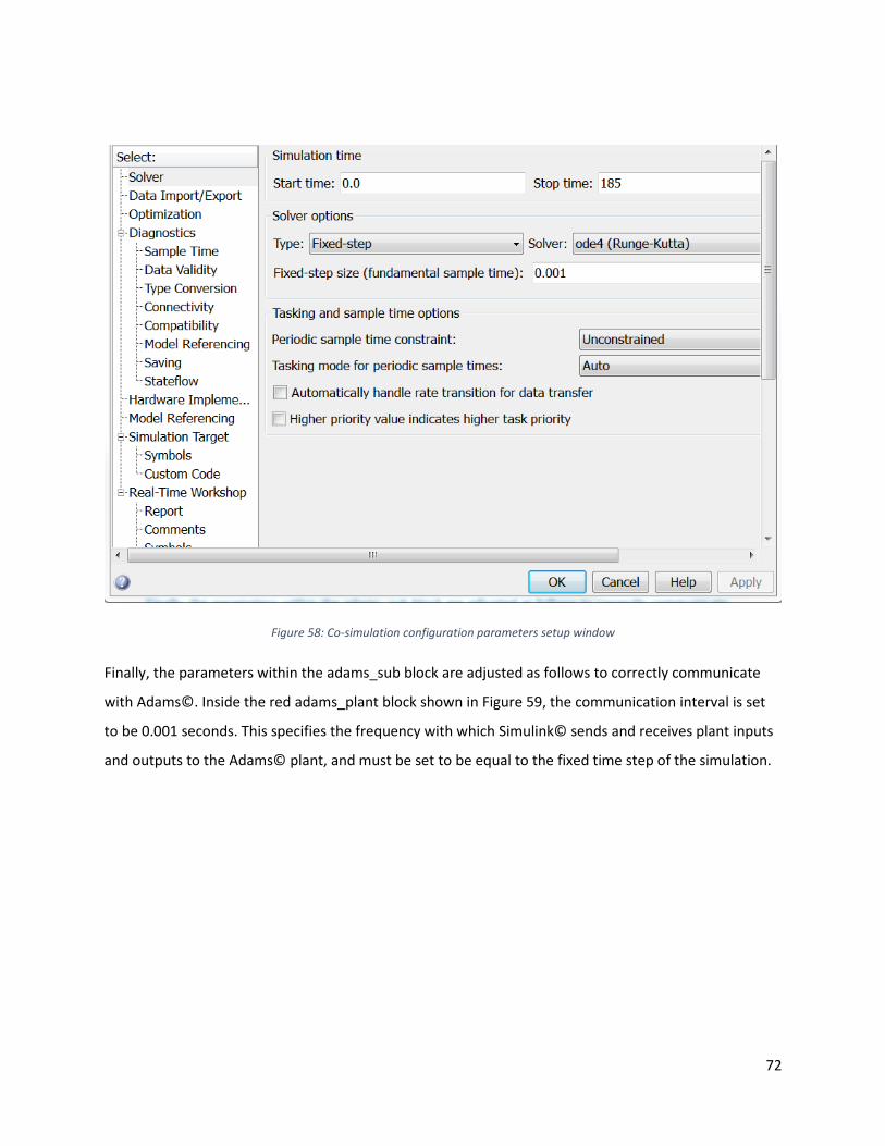
72

Figure 58: Co-simulation configuration parameters setup window

Finally, the parameters within the adams_sub block are adjusted as follows to correctly communicate

with Adams©. Inside the red adams_plant block shown in Figure 59, the communication interval is set

to be 0.001 seconds. This specifies the frequency with which Simulink© sends and receives plant inputs

and outputs to the Adams© plant, and must be set to be equal to the fixed time step of the simulation.

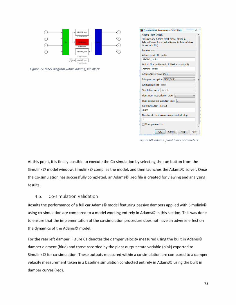
73

Figure 59: Block diagram within adams_sub block

Figure 60: adams_plant block parameters

At this point, it is finally possible to execute the Co-simulation by selecting the run button from the

Simulink© model window. Simulink© compiles the model, and then launches the Adams© solver. Once

the Co-simulation has successfully completed, an Adams© .req file is created for viewing and analyzing

results.

4.5. Co-simulation Validation

Results the performance of a full car Adams© model featuring passive dampers applied with Simulink©

using co-simulation are compared to a model working entirely in Adams© in this section. This was done

to ensure that the implementation of the co-simulation procedure does not have an adverse effect on

the dynamics of the Adams© model.

For the rear left damper, Figure 61 denotes the damper velocity measured using the built in Adams©

damper element (blue) and those recorded by the plant output state variable (pink) exported to

Simulink© for co-simulation. These outputs measured within a co-simulation are compared to a damper

velocity measurement taken in a baseline simulation conducted entirely in Adams© using the built in

damper curves (red).

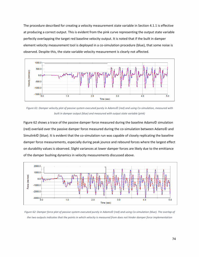
74

The procedure described for creating a velocity measurement state variable in Section 4.1.1 is effective

at producing a correct output. This is evident from the pink curve representing the output state variable

perfectly overlapping the target red baseline velocity output. It is noted that if the built in damper

element velocity measurement tool is deployed in a co-simulation procedure (blue), that some noise is

observed. Despite this, the state variable velocity measurement is clearly not affected.

Figure 61: Damper velocity plot of passive system executed purely in Adams© (red) and using Co-simulation, measured with

built in damper output (blue) and measured with output state variable (pink)

Figure 62 shows a trace of the passive damper force measured during the baseline Adams© simulation

(red) overlaid over the passive damper force measured during the co-simulation between Adams© and

Simulink© (blue). It is evident that the co-simulation run was capable of closely replicating the baseline

damper force measurements, especially during peak jounce and rebound forces where the largest effect

on durability values is observed. Slight variances at lower damper forces are likely due to the emittance

of the damper bushing dynamics in velocity measurements discussed above.

Figure 62: Damper force plot of passive system executed purely in Adams© (red) and using Co-simulation (blue). The overlap of

the two outputs indicates that the points in which velocity is measured from does not hinder damper force implementation

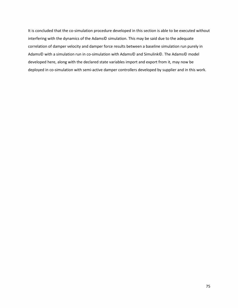
75

It is concluded that the co-simulation procedure developed in this section is able to be executed without

interfering with the dynamics of the Adams© simulation. This may be said due to the adequate

correlation of damper velocity and damper force results between a baseline simulation run purely in

Adams© with a simulation run in co-simulation with Adams© and Simulink©. The Adams© model

developed here, along with the declared state variables import and export from it, may now be

deployed in co-simulation with semi-active damper controllers developed by supplier and in this work.

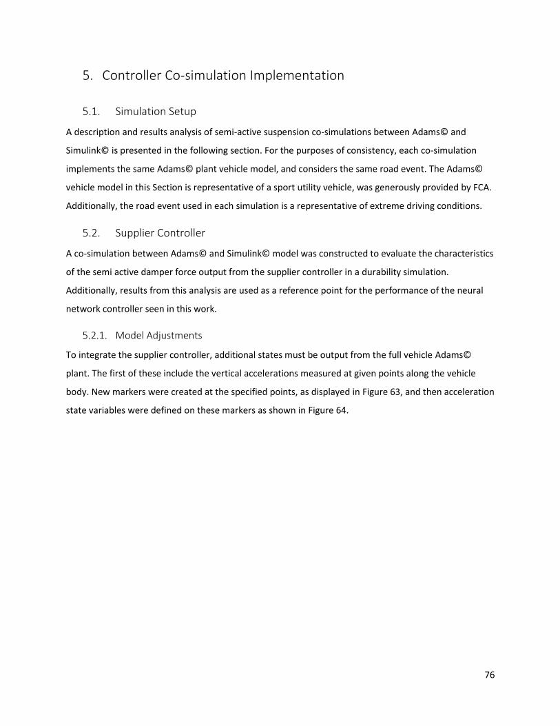
76

5. Controller Co-simulation Implementation

5.1. Simulation Setup

A description and results analysis of semi-active suspension co-simulations between Adams© and

Simulink© is presented in the following section. For the purposes of consistency, each co-simulation

implements the same Adams© plant vehicle model, and considers the same road event. The Adams©

vehicle model in this Section is representative of a sport utility vehicle, was generously provided by FCA.

Additionally, the road event used in each simulation is a representative of extreme driving conditions.

5.2. Supplier Controller

A co-simulation between Adams© and Simulink© model was constructed to evaluate the characteristics

of the semi active damper force output from the supplier controller in a durability simulation.

Additionally, results from this analysis are used as a reference point for the performance of the neural

network controller seen in this work.

5.2.1. Model Adjustments

To integrate the supplier controller, additional states must be output from the full vehicle Adams©

plant. The first of these include the vertical accelerations measured at given points along the vehicle

body. New markers were created at the specified points, as displayed in Figure 63, and then acceleration

state variables were defined on these markers as shown in Figure 64.

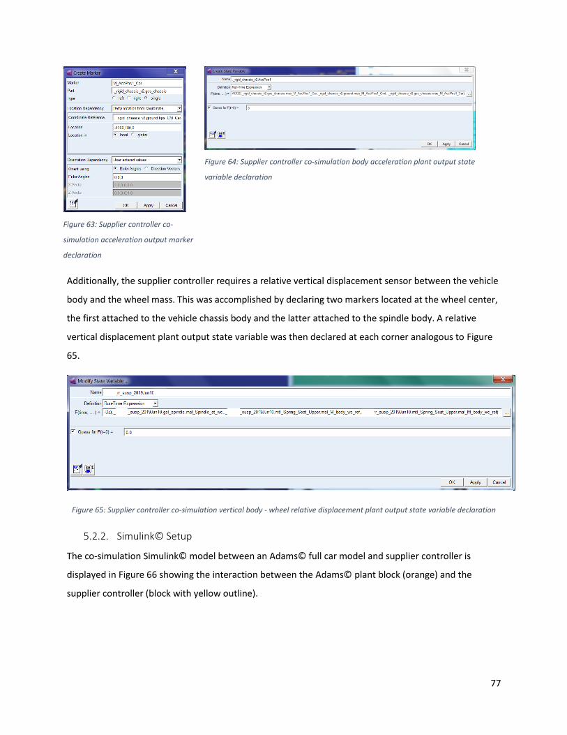
77

Figure 63: Supplier controller co-

simulation acceleration output marker

declaration

Figure 64: Supplier controller co-simulation body acceleration plant output state

variable declaration

Additionally, the supplier controller requires a relative vertical displacement sensor between the vehicle

body and the wheel mass. This was accomplished by declaring two markers located at the wheel center,

the first attached to the vehicle chassis body and the latter attached to the spindle body. A relative

vertical displacement plant output state variable was then declared at each corner analogous to Figure

65.

Figure 65: Supplier controller co-simulation vertical body - wheel relative displacement plant output state variable declaration

5.2.2. Simulink© Setup

The co-simulation Simulink© model between an Adams© full car model and supplier controller is

displayed in Figure 66 showing the interaction between the Adams© plant block (orange) and the

supplier controller (block with yellow outline).

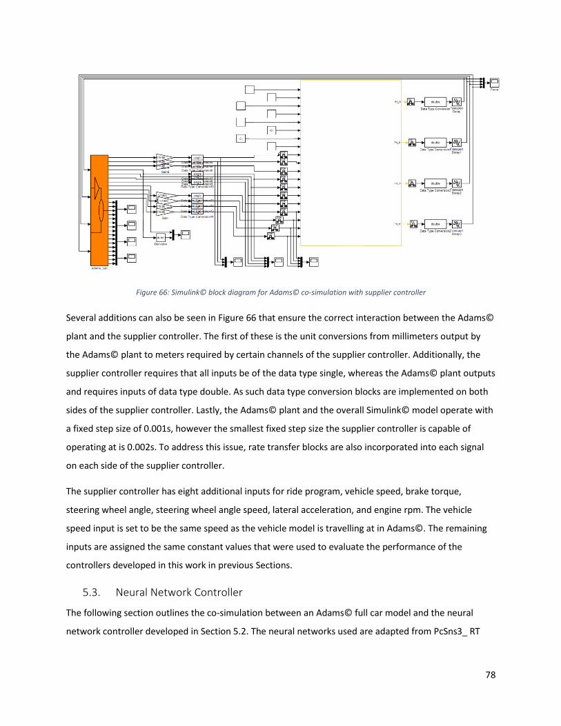
78

Figure 66: Simulink© block diagram for Adams© co-simulation with supplier controller

Several additions can also be seen in Figure 66 that ensure the correct interaction between the Adams©

plant and the supplier controller. The first of these is the unit conversions from millimeters output by

the Adams© plant to meters required by certain channels of the supplier controller. Additionally, the

supplier controller requires that all inputs be of the data type single, whereas the Adams© plant outputs

and requires inputs of data type double. As such data type conversion blocks are implemented on both

sides of the supplier controller. Lastly, the Adams© plant and the overall Simulink© model operate with

a fixed step size of 0.001s, however the smallest fixed step size the supplier controller is capable of

operating at is 0.002s. To address this issue, rate transfer blocks are also incorporated into each signal

on each side of the supplier controller.

The supplier controller has eight additional inputs for ride program, vehicle speed, brake torque,

steering wheel angle, steering wheel angle speed, lateral acceleration, and engine rpm. The vehicle

speed input is set to be the same speed as the vehicle model is travelling at in Adams©. The remaining

inputs are assigned the same constant values that were used to evaluate the performance of the

controllers developed in this work in previous Sections.

5.3. Neural Network Controller

The following section outlines the co-simulation between an Adams© full car model and the neural

network controller developed in Section 5.2. The neural networks used are adapted from PcSns3_ RT

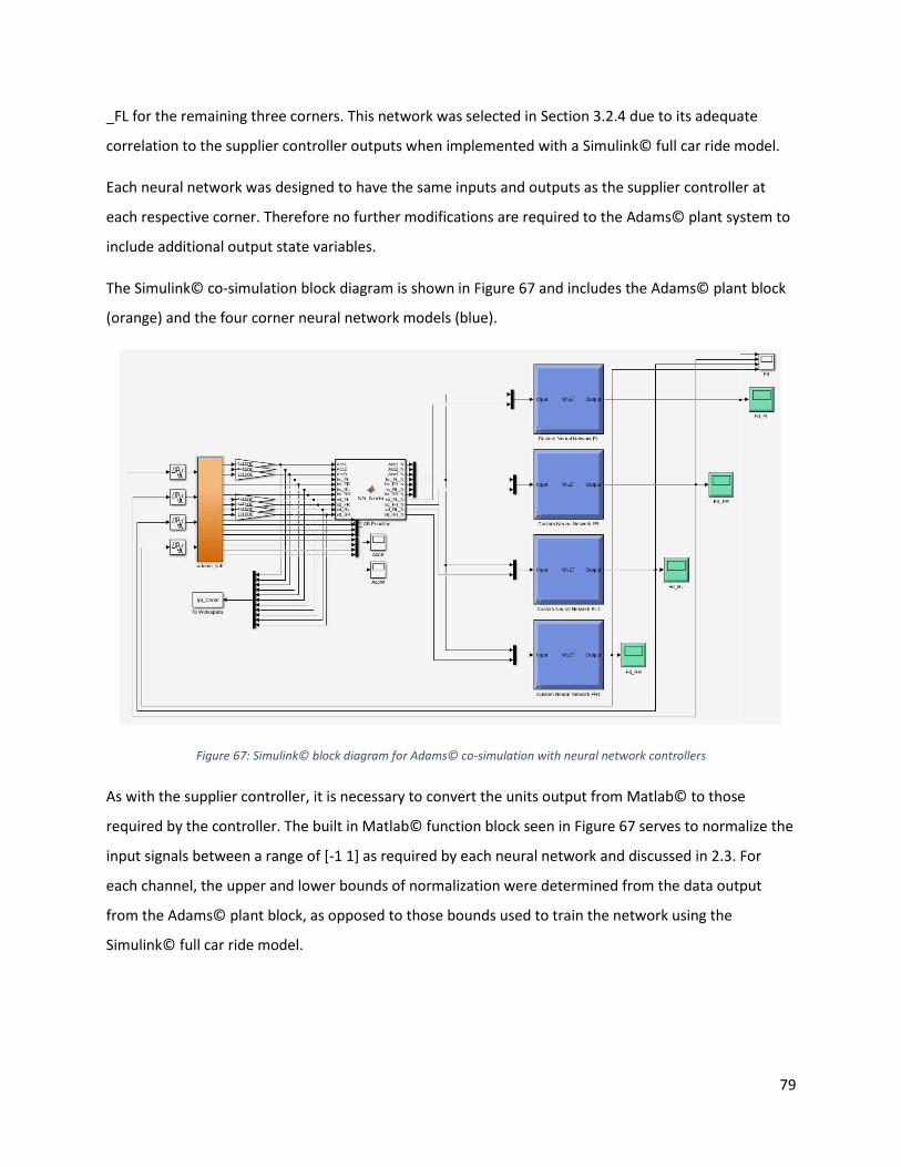
79

_FL for the remaining three corners. This network was selected in Section 3.2.4 due to its adequate

correlation to the supplier controller outputs when implemented with a Simulink© full car ride model.

Each neural network was designed to have the same inputs and outputs as the supplier controller at

each respective corner. Therefore no further modifications are required to the Adams© plant system to

include additional output state variables.

The Simulink© co-simulation block diagram is shown in Figure 67 and includes the Adams© plant block

(orange) and the four corner neural network models (blue).

Figure 67: Simulink© block diagram for Adams© co-simulation with neural network controllers

As with the supplier controller, it is necessary to convert the units output from Matlab© to those

required by the controller. The built in Matlab© function block seen in Figure 67 serves to normalize the

input signals between a range of [-1 1] as required by each neural network and discussed in 2.3. For

each channel, the upper and lower bounds of normalization were determined from the data output

from the Adams© plant block, as opposed to those bounds used to train the network using the

Simulink© full car ride model.

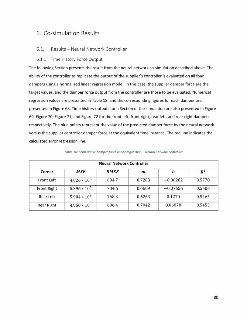
80

6. Co-simulation Results

6.1. Results – Neural Network Controller

6.1.1 Time History Force Output

The following Section presents the result from the neural network co-simulation described above. The

ability of the controller to replicate the output of the supplier’s controller is evaluated on all four

dampers using a normalized linear regression model. In this case, the supplier damper force are the

target values, and the damper force output from the controller are those to be evaluated. Numerical

regression values are presented in Table 18, and the corresponding figures for each damper are

presented in Figure 68. Time history outputs for a Section of the simulation are also presented in Figure

69, Figure 70, Figure 71, and Figure 72 for the front left, front right, rear left, and rear right dampers

respectively. The blue points represent the value of the predicted damper force by the neural network

versus the supplier controller damper force at the equivalent time instance. The red line indicates the

calculated error regression line.

Table 18: Semi-active damper force linear regression – Neural network controller

Neural Network Controller

Corner 𝑴𝑺𝑬 𝑹𝑴𝑺𝑬 𝒎 𝒃 𝑹𝟐

Front Left 4.826 ∗ 105 694.7 0.7283 −0.06282 0.5778

Front Right 5.396 ∗ 105 734.6 0.6609 −0.07656 0.5606

Rear Left 5.904 ∗ 105 768.3 0.6263 0.1270 0.5465

Rear Right 4.850 ∗ 105 696.4 0.7042 0.06878 0.5455

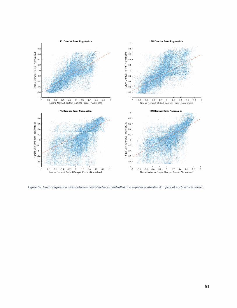
81

Figure 68: Linear regression plots between neural network controlled and supplier controlled dampers at each vehicle corner.

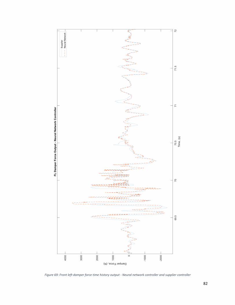
82

Figure 69: Front left damper force time history output - Neural network controller and supplier controller

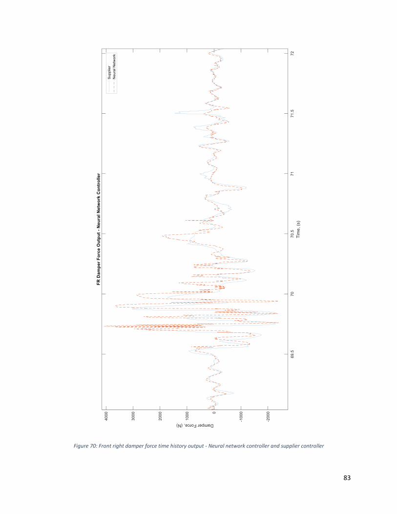
83

Figure 70: Front right damper force time history output - Neural network controller and supplier controller

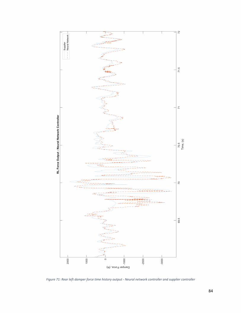
84

Figure 71: Rear left damper force time history output - Neural network controller and supplier controller

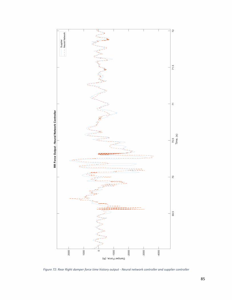
85

Figure 72: Rear Right damper force time history output - Neural network controller and supplier controller

86

6.1.2 Durability Calculations

A durability analysis was then conducted in order to calculate the damage incurred along the axis of the

dampers. The results for the supplier controller are compared to the neural network controller below.

Maximum and minimum damper axial loads determined in the co-simulation are displayed in Table 19

and Table 20, for the supplier’s controller and neural network controller respectively. They are then

compared visually in Figure 73.

Damage is a parameter representing the amount that a specific loading scenario contributes to a

component reaching its fatigue life. It is useful for comparing the effects that changes in topology or

setup of the vehicle have on durability. As such, this parameter is useful in this case for evaluating how

well a controller matches the outputs of a supplier’s controller, as damage values should be the same

for each. Calculated damage values for the damper axial loads for 100 cycles of the co-simulation are

displayed in Table 21 and Table 22, for the supplier’s controller and neural network controller

respectively. The ratios are then compared visually in Figure 74.

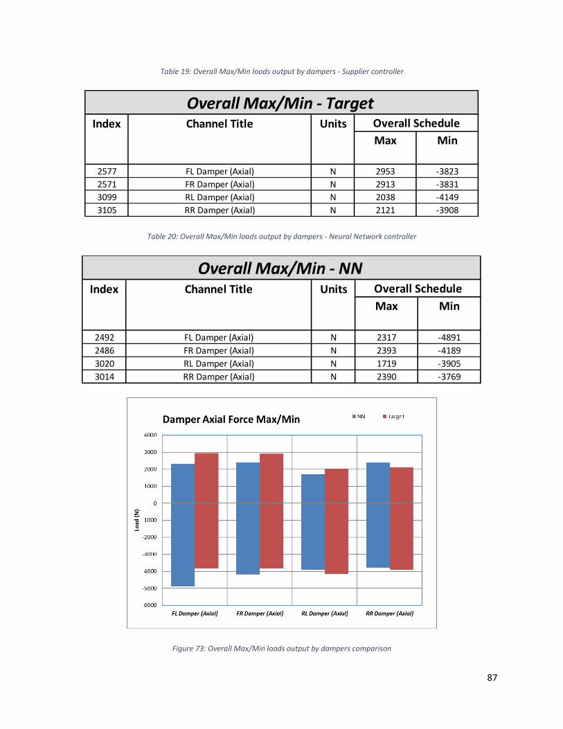
87

Table 19: Overall Max/Min loads output by dampers - Supplier controller

Table 20: Overall Max/Min loads output by dampers - Neural Network controller

Figure 73: Overall Max/Min loads output by dampers comparison

Index Channel Title Units

Max Min

2577 FL Damper (Axial) N 2953 -3823

2571 FR Damper (Axial) N 2913 -3831

3099 RL Damper (Axial) N 2038 -4149

3105 RR Damper (Axial) N 2121 -3908

Overall Max/Min - TargetOverall Schedule

Index Channel Title Units

Max Min

2492 FL Damper (Axial) N 2317 -4891

2486 FR Damper (Axial) N 2393 -4189

3020 RL Damper (Axial) N 1719 -3905

3014 RR Damper (Axial) N 2390 -3769

Overall Max/Min - NNOverall Schedule

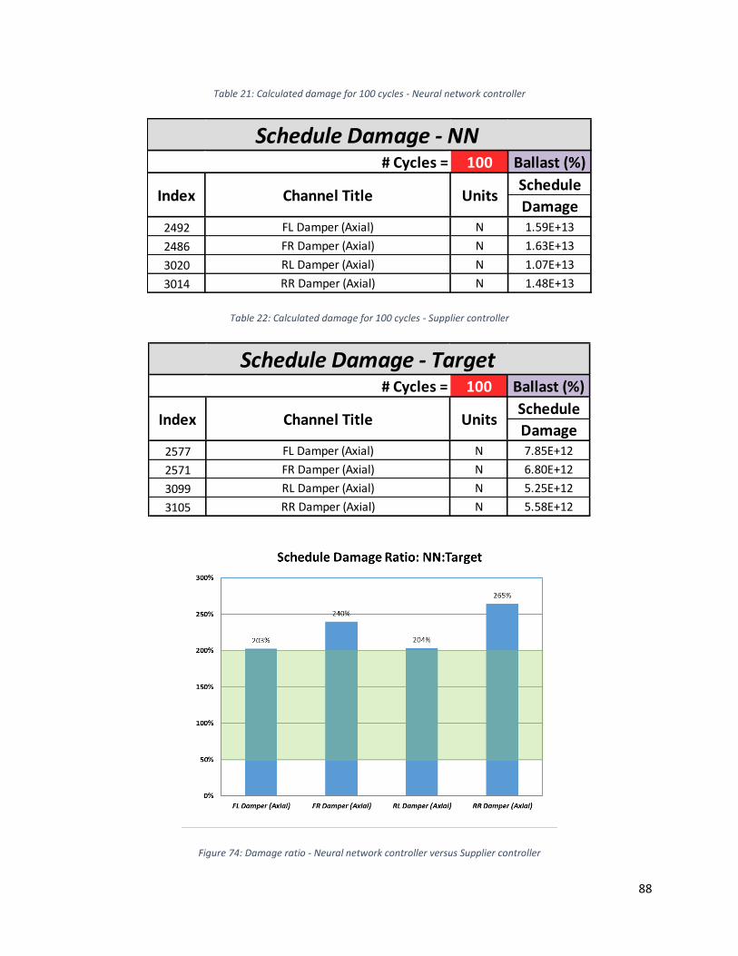
88

Table 21: Calculated damage for 100 cycles - Neural network controller

Table 22: Calculated damage for 100 cycles - Supplier controller

Figure 74: Damage ratio - Neural network controller versus Supplier controller

# Cycles = 100 Ballast (%)

Schedule

Damage2492 FL Damper (Axial) N 1.59E+13

2486 FR Damper (Axial) N 1.63E+13

3020 RL Damper (Axial) N 1.07E+13

3014 RR Damper (Axial) N 1.48E+13

Schedule Damage - NN

Index Channel Title Units

# Cycles = 100 Ballast (%)

Schedule

Damage2577 FL Damper (Axial) N 7.85E+12

2571 FR Damper (Axial) N 6.80E+12

3099 RL Damper (Axial) N 5.25E+12

3105 RR Damper (Axial) N 5.58E+12

Schedule Damage - Target

Index Channel Title Units

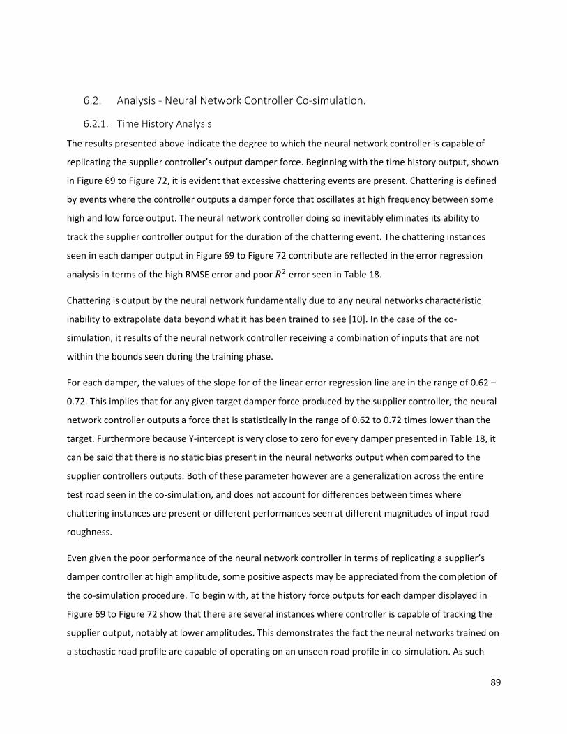
89

6.2. Analysis - Neural Network Controller Co-simulation.

6.2.1. Time History Analysis

The results presented above indicate the degree to which the neural network controller is capable of

replicating the supplier controller’s output damper force. Beginning with the time history output, shown

in Figure 69 to Figure 72, it is evident that excessive chattering events are present. Chattering is defined

by events where the controller outputs a damper force that oscillates at high frequency between some

high and low force output. The neural network controller doing so inevitably eliminates its ability to

track the supplier controller output for the duration of the chattering event. The chattering instances

seen in each damper output in Figure 69 to Figure 72 contribute are reflected in the error regression

analysis in terms of the high RMSE error and poor 𝑅2 error seen in Table 18.

Chattering is output by the neural network fundamentally due to any neural networks characteristic

inability to extrapolate data beyond what it has been trained to see [10]. In the case of the co-

simulation, it results of the neural network controller receiving a combination of inputs that are not

within the bounds seen during the training phase.

For each damper, the values of the slope for of the linear error regression line are in the range of 0.62 –

0.72. This implies that for any given target damper force produced by the supplier controller, the neural

network controller outputs a force that is statistically in the range of 0.62 to 0.72 times lower than the

target. Furthermore because Y-intercept is very close to zero for every damper presented in Table 18, it

can be said that there is no static bias present in the neural networks output when compared to the

supplier controllers outputs. Both of these parameter however are a generalization across the entire

test road seen in the co-simulation, and does not account for differences between times where

chattering instances are present or different performances seen at different magnitudes of input road

roughness.

Even given the poor performance of the neural network controller in terms of replicating a supplier’s

damper controller at high amplitude, some positive aspects may be appreciated from the completion of

the co-simulation procedure. To begin with, at the history force outputs for each damper displayed in

Figure 69 to Figure 72 show that there are several instances where controller is capable of tracking the

supplier output, notably at lower amplitudes. This demonstrates the fact the neural networks trained on

a stochastic road profile are capable of operating on an unseen road profile in co-simulation. As such

90

this validates the stochastic road profile training method, but reinforces the concept that the stochastic

road profile must contain a range of inputs expected to be seen in the environment the neural network

is to be deployed in. Furthermore, Figure 69 to Figure 72 in addition to Table 18 show a consistent

performance across all four dampers. This validates the method of selecting an optimally performing

network architecture for one damper, and then creating controllers for the remaining three corners by

adapting the best performing network.

6.2.2. Durability Analysis

As the overall purpose of this work is to improve the fidelity of durability simulations by improving the

quality of the model they are based on. As such, it was necessary to examine the results often calculated

in durability simulations at FCA.

An important aspect of a durability analysis is the maximum loads experienced by a component, which is

often used later in the design phase of the vehicle. As can be seen in Figure 73, the maximum and

minimum loads produced by the neural network controller are close to those values produced by the

supplier controller. The maximum percent difference of 27.9% is seen in the jounce motion of the Front

left damper curve. Despite the remaining maximum and minimum loads produced by the neural

network controller being much closer to those produced by the supplier controller, this analysis does

not include the time at which these loads are generated. Furthermore, there is not a common trend in

the error between each damper corner. In certain cases seen in Figure 73, the neural network controller

both overestimates targets on certain dampers and underestimates targets on others.

Another important parameter determined in durability simulations is the damage calculated on several

joints and components. Often calculated as the sum of several cycles over multiple test roads at

different loading conditions, for this analysis only 100 cycles of the road seen in the durability simulation

are considered.

Figure 74 displays the ratio of the damage accrued with the supplier controller versus the neural

network controller. The zone shaded in green denotes the region that would normally be considered to

be an acceptable correlation. In this case, the damage values output at each damper are over 200%

higher than those of the target value. This is again likely an effect of the chattering that can be seen in

the time history plots in Section 6.1.1. Despite the maximum and minimum values being similar, the

excessive high frequency transitioning between random high and low force output values inflates the

damage values calculated. Because the neural network controller was not able to replicate damage

91

values in this instance, it is not possible to deem this specific network suitable for further use in

durability simulations.

As concluding remark, the entirety of the co-simulation procedure shown here between a full car

Adams© model and a Simulink© neural network controller is possible to be completed successfully.

Unfortunately, the errors incurred in the construction of the neural networks itself rendered it

unsuitable for deployment in durability simulations. As possible solutions to develop an improved neural

network are presented in Section 7.2.1.

92

7. Conclusions and Recommendations

7.1. Conclusions

7.1.1. Clipped Optimal Controller

From both the literature review and the initial examination of the clipped optimal controller using a

quarter car model in Section 3.1.1, it is possible to conclude that a clipped optimal controller has a wide

range of adjustability in terms of comfort or handling performance. In addition, Section 3.1.1

demonstrates that a clipped optimal controller well outperforms a passive system.

Unfortunately, for the purposes of this work, it must be concluded that the chosen clipped optimal

controller structure cannot be adjusted to match the target performance of a supplier controller. This is

most likely due to the fact that a clipped optimal controller operates with a fixed set of optimally chosen

gains, which do not adapt to changing input conditions. Therefore it must be concluded that the supplier

controller is of a more advanced structure, which the clipped optimal controller is not capable of

replicating.

7.1.2. Neural Network Controller

One of the first and key conclusions that can be made from Section 3.2 is the sensitivity of a neural

network to the type of training data that is used. A neural network replicating a supplier’s adaptive

damper system will fail to perform acceptably if the input road used to acquire the training data from a

supplier controller is not representative of the environment the neural network controller is expected to

perform in. As such, it is concluded from Section 3.2.4 that the creation of a stochastic road profile that

replicates the power spectral density of the desired road profile is an effective way of creating useful

training data.

Several analyses were conducted throughout Section 3.2 that examined the effects of different network

architecture. From each case, it was determined that increasing the number of hidden layers was not

effective in improving the accuracy of the neural network. Furthermore, it was determined that

increasing the number of hidden layer perceptrons to beyond that specified by Komolgrov’s theorem

proved to also decrease both the training speed of the neural network and the accuracy of results.

Finally, the inclusion of history data points as inputs to the neural network to account for hysteresis

effects displayed worse results then a neural network operating with inputs only from the current time

step for the stochastic road profile training data seen in Section 3.2.4.

93

In terms of training a neural network to replicate a supplier’s semi-active damper controller, it must be

said that the results presented in this Section serve more as guidelines. Any additional attempts going

forward would require some amount of trial and error to determine a network architecture capable of

producing the best results for the type of vehicle, controller, and environment it is desired to perform in.

7.1.3. Sliding Mode Controller

At a fundamental level, it can be concluded from the results shown in Section 3.3.1.1 that for a quarter

car model, a sliding mode controller greatly improves the comfort in terms of vertical body acceleration.

The sliding mode controller was then expanded to a full car ride model using two methods, the first

being a controller based on four quarter car models, and the second being a controller based on two

half car models. In terms of tracking the target supplier’s controller output, it can be concluded from the

results shown in Section 3.3.3.3 that the quarter car based controller provided superior performance.

The results from the quarter car based controller were in fact the closest match to the supplier

controller considered in this work in terms of the RMSE value.

Despite this positive conclusion, the sliding mode quarter car based controller was not implemented

into the co-simulation with Adams© due to the requirement of vertical displacement states of both the

body and wheel masses relative to the road as inputs. Because of this issue, further work discussed in

Section 7.2.2 needs to be completed before a sliding mode may be implemented.

7.1.4. Durability Simulation Implementation

The culmination of Section 4 shows how that co-simulation between Adams© and Simulink© can be

used effectively to implement a passive damper force on a vehicle without introducing errors and

compromising the integrity of the simulation. From this, it is concluded that co-simulation is a viable way

to implement semi-active damper systems in durability simulations.

The beginning of Section 5 demonstrates how the co-simulation procedure is expanded from passive

damping to include a supplier damper controller. From there, the neural network controller developed

in Section 3.2.4 is also implemented using co-simulation over the same road profile. Several conclusions

were made by comparing the results of the neural network controller to the supplier controller. The first

is that, while requiring further revisions, the method of training the neural network in Simulink© was

able to create a neural network that could then replicate the output of the supplier’s damper controller.

It is also concluded from the chattering instances seen with the neural network that the training data

94

has a large effect on the quality of results. Because of this, steps must be taken to modify the data used

for neural network training is described in Section 7.2.1 in order to improve network performance.

7.1.5. Overall

Overall, two main conclusions may be drawn from this work. First, it is concluded from both Sections

3.2.4 and 3.3.3.1 that it is indeed possible to replicate the performance of a common supplier’s

controller using either neural networks or sliding mode control respectively. From the results in Section

3.3.3.1, it is concluded that the sliding mode control algorithm is most likely equivalent to that used in

the supplier’s controller examined in this work. Furthermore, some adjustment of the controller’s

physical parameters tuning weights make this control structure suitable to perform well in front end

durability simulations before the functionality of the actual damper controller is determined.

The second overall conclusion that may be drawn is that it is possible to replicate the effects of a semi

active damper system in a durability analysis using co-simulation. Despite not being able to implement

any control algorithm requiring an observer, It is concluded from Section 5 that either a supplier semi-

active damper system, or a system developed from literature may be effectively implemented in

Adams© using co-simulation with Simulink ©.

7.2. Recommendations

7.2.1. Neural Network Controller Despite it being successfully shown that a neural network may be integrated into a durability simulation

from a functional point of view, the particular neural network itself used in this case was unsuccessful at

producing an output that is suitable for analysis in a practical setting.

A potential improvement would be retraining the neural network controller using input and output

training data obtained from the supplier controller simulated with an Adams© vehicle model as

opposed to a Simulink© full vehicle ride model. By doing so, it may be possible to construct a neural

network controller capable of performing without chattering events as errors introduced by using a

different model for training will be eliminated.

The advantage to using training data from the Adams© vehicle model is that errors incurred from using

the Simulink© full car ride model would be eliminated. These types of errors include the fact that the

Simulink© full car ride model neglects most kinematic effects, yaw motions, effects from steering, and

several others. Using the Adams© vehicle model and eliminating these errors would help to ensure that

95

inputs to the controller in durability simulations would be more consistent with those seen in the

training data.

The difficulty with executing this procedure would be the development of a stochastic road input for the

Adams© model that is representative of the road profiles seen in durability simulations, without using

an existing road profile. The risk of using a measured road profile would be that the trained network

memorizes the training data and is unable to perform on any new road profile. In addition, the newly

developed stochastic road profile would have to be done in a manner that ensures that all possible

inputs to the neural network controller do not lie outside of the training dataset. In Section 3.2.4, it was

ensured that the stochastic road input had the same Amplitude spectrum and PSD as a road profile

commonly seen in durability simulations, however an improvement be to perform this analysis for each

input channel to the neural network as opposed to just the road profile.

7.2.2. Sliding Mode Controller The quarter car sliding mode controller developed in Section 3.3.2.1 and tested in 3.3.3.1 showed the

most promising results when it came to replicating the supplier’s controller’s damper force output.

Additionally, the structure of a sliding mode controller would make it very straight forward to adapt to

future projects by modifying the physical vehicle parameters used by the controller.

Unfortunately, the requirement that this controller have as inputs the sprung and unsprung mass

displacement relative to the road displacement resulted in it not being able to be evaluated with Co-

simulation. This was due to the fact that Adams© is unable to directly output these states.

The clear solution to this problem reserved for future work is the development of some form of state

observer. This observer would take measurable outputs from Adams©, and using a simplified state

space model of the Adams© model, output a full state vector at each time step during the simulation.

A promising Kalman state observer is described in [9] where the road input is considered to be a known

input acting on the plant model. Unfortunately, the complexity of a full car state space model and the

requirement that the variance of the magnitude of the road input be known makes this observer

cumbersome to implement.

7.2.3. Overall The culmination of this work has shown two separate, yet equally important aspects required to

improve the quality of models used in durability simulations. The first is that it is possible to design in

Simulink© a control structure that performs in a manner that replicates controllers developed by

96

external suppliers, as shown in Sections 3.2.4 and 3.3.3.1. The second being that it is possible to

implement this semi-active damper controller in Adams© using co-simulation with Simulink©, as shown

in Chapter 4.

Going forward, and applying the recommendations explained in Sections 7.2.1 and 7.2.2, it should be

possible to implement this work in the early stages of development on new platforms. This will be useful

in a durability analysis to estimate the performance of a supplier’s controller in the event that the

supplier or the system is unknown. Doing so will provide earlier insights to the loads and damage that

will be expected with the implementation of a semi-active suspension system. Furthermore, it may be

possible FCA to determine the desired characteristics of a semi-active suspension system, rather than

relying on a supplier to create a system.

97

References

[1] G. P. Koch, "Adaptive Control of Mechatronic Vehicle Suspension Systems," Technische Universitat

Munchen, Munich , 2010.

[2] J. L. Johrendt, "Optimization of Road Test Simulation Using Neural Network Modeling Techniques,"

Electronic Thesis and Dissertations, 5248, University of Windsor, Windsor, Ontario, 2005.

[3] D. Karnopp and M. Crospy, "System for Controlling the Transmission of Energy between Spaced

Members". United States of America Patent 3,807,678, April 1974.

[4] A. Mulla, S. Jalwadi and D. Unanune, "Performance Analysis of Skyhook, Groundhook, and Hybrid

Control Strategies on Semi-Active Suspension," International Journal of Current Engineering and

Technology, no. 3, pp. 265-269, 2014.

[5] Y. Liu, T. P. Waters and M. J. Brennan, "A Comparison of semi-active damping control strategies for

vibration isolation of harmonic disturbances," Journal of Sound and Vibration, vol. 280, pp. 21-39,

2005.

[6] G. Slaski and M. Maciejewski, "Skyhook and Fuzzy Logic Controller of a Semi Active Vehicle

Suspension," Poznan University of Technology, Institute of Machines and Motor Vehicles, Poznań,

Poland, 2011.

[7] S. Rasal, J. Jaganmohan, S. Agashe and K. P. Wani, "Implementation of Fuzzy Logic Control in

Semiactive Suspension for a Vehicle Using MATLAB SIMULINK," SAE Techincal Paper, vol. 28, no.

035, 2016.

[8] P. Brezas, M. C. Smith and W. Hoult, "A clipped-optimal control algorithm for semi-active

suspensions: Theory and evaluations," Automatica, vol. 53, pp. 188-194, 2014.

[9] P. Brezas and M. C. Smith, "Linear Quadratic Optimal and Risk-Sensitive Control for a Vehicle

Active Suspensions," IEEE Transactions on Control Systems Technology, vol. 22, no. 2, pp. 543-556,

2013.

[10] S. Samarasinghe, Neural Networks for Applied Sciences and Engineering, New York: Auerbach

Publications, 2007.

[11] Y. Chen, "Skyhook Surface Sliding Mode Control on Semi-Active Vehicle Suspension System for

Ride Comfort Enhancement," Engineering, 1 (1), pp. 22-32, 2009.

98

[12] H. Metered, P. Bonello and S. O. Oyadiji, "An investigation into the use of neural networks for the

semi-active control of a magnetorheologically damped vehicle suspension," School of Mechanical,

Aerospace and Civil Engineering, The University of Manchester, Manchester, UK, 2010.

[13] H. Zhang, E. Wang, N. Zhang, F. Min, R. Subash and S. Chunyi, "Semi-Active Sliding Mode Control of

Vehicle Suspension with Magneto-rheological Damper," Chinese Journal of Mechanical

Engineering, vol. 28, no. 1, pp. 63-76, 2015.

[14] A. Tonoli, Writer, Car Body Design and Aerodynamics - Stochasitc Road Profile Lecture.

[Performance]. Politecnico di Torino, 2019.

[15] K. Hassani and W.-S. Lee, "Optimal Tuning of Linear Quadratic Regulators Using Quantum Particle

Swarm Optimization," in Int. Conference of Control, Dynamic Systems, and Robotics, Ottawa,

Ontario, Canada, May 15-16, 2014.

[16] Mathworks Inc. , "patternsearch - Mathworks Documentation," Mathworks Inc. , 2019. [Online].

Available: https://www.mathworks.com/help/gads/patternsearch.html. [Accessed 24 February

2019].

[17] V. Kurkova, "Kolmogrov's Theorem is Relevant," Neural Computation, vol. 3, no. 4, pp. 617-622,

1991.

[18] R. Goldman, "Development of a Rollover-Warning Device for Road Vehicles," Ph.D. Thesis,

Pennsylvania State University, 2001.

[19] MSC Software, Adams Tutorial Kit for Mechanical Engineering Courses (Third Edition), MSC

Software.

[20] M. Kaldas, K. Caliskan, R. Henze and F. Kucukay, "Preview Enhanced Rule-Optimized Fuzzy Logic

Damper Controller," SAE International Journal Passenger Cars - Mechanical Systems, vol. 7, no. 2,

pp. 804-815, 2014.

[21] B. Messner, D. Tillbury, R. Hill and J. Talyor, "Control Tutorials For Matlab and Simulink -

Suspension: Simulink Modelling," University of Michigan, Carnagie Melon University, Detroit

Mercy University , 2014. [Online]. Available:

http://ctms.engin.umich.edu/CTMS/index.php?example=Suspension&section=SimulinkModeling.

[Accessed 22 01 2018].

[22] Fiat Chrysler Automobiles North America, "2018 Jeep Grand Cherokee Specifications," Fiat Chrysler

Automobiles North America, Auburn Hills, Michigan, 2018.

[23] J. Maiorana, "Active Suspension Simulation Through Software Interfacing," Electronic Theses

Dissertations 6954, Univerisity of Windsor , 2004.

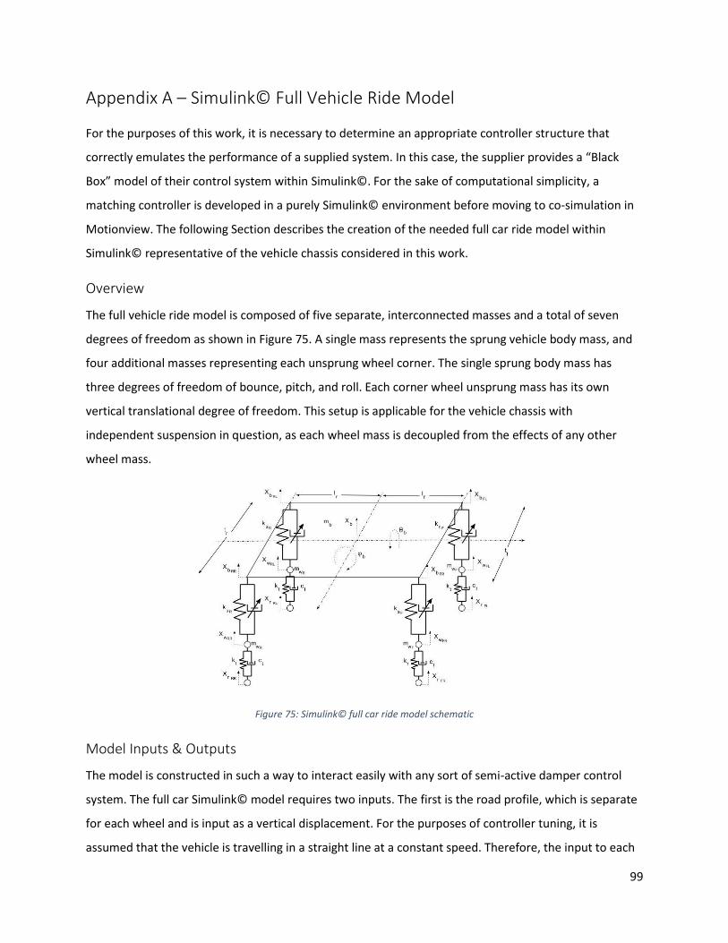
99

Appendix A – Simulink© Full Vehicle Ride Model

For the purposes of this work, it is necessary to determine an appropriate controller structure that

correctly emulates the performance of a supplied system. In this case, the supplier provides a “Black

Box” model of their control system within Simulink©. For the sake of computational simplicity, a

matching controller is developed in a purely Simulink© environment before moving to co-simulation in

Motionview. The following Section describes the creation of the needed full car ride model within

Simulink© representative of the vehicle chassis considered in this work.

Overview

The full vehicle ride model is composed of five separate, interconnected masses and a total of seven

degrees of freedom as shown in Figure 75. A single mass represents the sprung vehicle body mass, and

four additional masses representing each unsprung wheel corner. The single sprung body mass has

three degrees of freedom of bounce, pitch, and roll. Each corner wheel unsprung mass has its own

vertical translational degree of freedom. This setup is applicable for the vehicle chassis with

independent suspension in question, as each wheel mass is decoupled from the effects of any other

wheel mass.

Figure 75: Simulink© full car ride model schematic

Model Inputs & Outputs

The model is constructed in such a way to interact easily with any sort of semi-active damper control

system. The full car Simulink© model requires two inputs. The first is the road profile, which is separate

for each wheel and is input as a vertical displacement. For the purposes of controller tuning, it is

assumed that the vehicle is travelling in a straight line at a constant speed. Therefore, the input to each

100

rear wheel is the same as its respective front wheel, but delayed a time period according to the vehicle’s

speed and wheelbase. The left and right wheels may be excited with different road profiles, as is found

in real world situations. The second input required is that of the damper force values for each corner

that is output from the controller being used.

An additional motivation to use Simulink© for initial controller tuning is the ease of which that any

model state may be extracted as an output from the model, without requiring the use of an observer.

Common output examples include body acceleration bounce, roll and pitch components �̈�𝑏 , �̈�𝑏 , �̈�𝑏,

relative damper displacement: 𝑧𝑏 − 𝑧𝑤, and of course damper velocity: �̇�𝑏 − �̇�𝑤.

Equations of Motion

Full car ride model Equations of motion are described in several sources but very thoroughly presented

in [20], are derived from the free body diagrams of the sprung vehicle body lumped mass, and each of

the unsprung wheel lumped masses .

Beginning with considering the unsprung wheel mass, the following Equation of motion may be

constructed.

𝑚𝑤𝑖 �̈�𝑤𝑖 = 𝐹𝑆𝐷𝑖 − 𝑘𝑡(𝑧𝑤𝑖 − 𝑧𝑟𝑖) − 𝑐𝑡(�̇�𝑤𝑖 − �̇�𝑟𝑖) (46)

Where 𝑖 = 𝐹𝐿, 𝐹𝑅, 𝑅𝐿, 𝑅𝑅, corresponding to the front left, font right, rear left, rear right wheel

respectively.

The interactions between each individual wheel and the vehicle body itself are related by the force term

applied between each body, which for each corner, may be denoted as follows.

𝐹𝑆𝐷𝑖 = 𝑢𝑑𝑖 + 𝑘𝑆𝑖(𝑧𝑏𝑖 − 𝑧𝑤𝑖) (47)

Moving to the sprung vehicle body mass, the following Equations of motion denoting the bounce, roll

and pitch motions are created.

𝑚𝑏�̈�𝑏 = −𝐹𝑆𝐷𝐹𝐿 − 𝐹𝑆𝐷𝐹𝑅 − 𝐹𝑆𝐷𝑅𝐿 − 𝐹𝑆𝐷𝑅𝑅 (48)

𝐼𝑏𝑅𝑜𝑙𝑙�̈�𝑏 = −𝐹𝑆𝐷𝐹𝐿 ∗1

2𝑡𝑓 + 𝐹𝑆𝐷𝐹𝑅 ∗

1

2𝑡𝑓 − 𝐹𝑆𝐷𝑅𝐿 ∗

1

2𝑡𝑟 + 𝐹𝑆𝐷𝑅𝑅 ∗

1

2𝑡𝑟 (49)

101

𝐼𝑏𝑃𝑖𝑡𝑐ℎ�̈�𝑏 = 𝐹𝑆𝐷𝐹𝐿 ∗ 𝑙𝑓 + 𝐹𝑆𝐷𝐹𝑅 ∗ 𝑙𝑓 − 𝐹𝑆𝐷𝑅𝐿 ∗ 𝑙𝑟 − 𝐹𝑆𝐷𝑅𝑅 ∗ 𝑙𝑟 (50)

Finally, it is necessary to relate the body displacements in bounce, pitch, and roll back to vertical

displacements at each wheel corner as follows.

𝑧𝑏𝐹𝐿 = 𝑧𝑏 + 𝜃 ∗1

2𝑡𝑓 − 𝜙 ∗

1

2𝑙𝑓 (51)

𝑧𝑏𝐹𝑅 = 𝑧𝑏 − 𝜃 ∗1

2𝑡𝑓 −𝜙 ∗

1

2𝑙𝑓 (52)

𝑧𝑏𝑅𝐿 = 𝑧𝑏 + 𝜃 ∗1

2𝑡𝑟 + 𝜙 ∗

1

2𝑙𝑟 (53)

𝑧𝑏𝑅𝑅 = 𝑧𝑏 − 𝜃 ∗1

2𝑡𝑟 +𝜙 ∗

1

2𝑙𝑟 (54)

Simulink© Block Architecture

Using the Equations of motion described in the previous subSection, various blocks from the Simulink©

Library are used to construct the full car ride model. For each set of Equations shown above, a

Simulink© subsystem is constructed.

For each vehicle corner, the Equation of motion for the wheel mass shown in Equations (46) and (47) is

constructed in Simulink© as follows. The architecture shown below is a modification of the quarter car

model presented in [21].

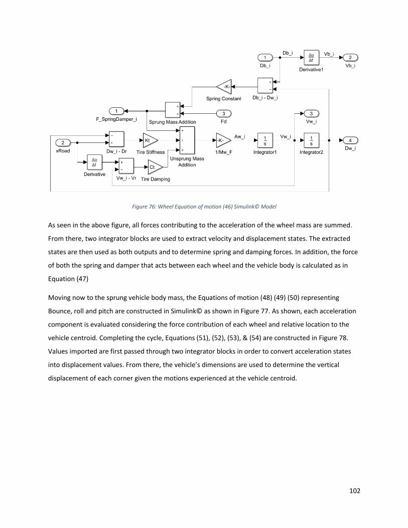
102

Figure 76: Wheel Equation of motion (46) Simulink© Model

As seen in the above figure, all forces contributing to the acceleration of the wheel mass are summed.

From there, two integrator blocks are used to extract velocity and displacement states. The extracted

states are then used as both outputs and to determine spring and damping forces. In addition, the force

of both the spring and damper that acts between each wheel and the vehicle body is calculated as in

Equation (47)

Moving now to the sprung vehicle body mass, the Equations of motion (48) (49) (50) representing

Bounce, roll and pitch are constructed in Simulink© as shown in Figure 77. As shown, each acceleration

component is evaluated considering the force contribution of each wheel and relative location to the

vehicle centroid. Completing the cycle, Equations (51), (52), (53), & (54) are constructed in Figure 78.

Values imported are first passed through two integrator blocks in order to convert acceleration states

into displacement values. From there, the vehicle’s dimensions are used to determine the vertical

displacement of each corner given the motions experienced at the vehicle centroid.

103

Figure 77: Vehicle body Equations of motion (48), (49), & (50) Simulink© model

Figure 78: Centroid accelerations to corner displacement conversion Simulink© block

The above figures all represent the three key subsystems that comprise the full car ride model. The

complete full car ride model layout is shown in Figure 79. Connectivity is shown between input damper

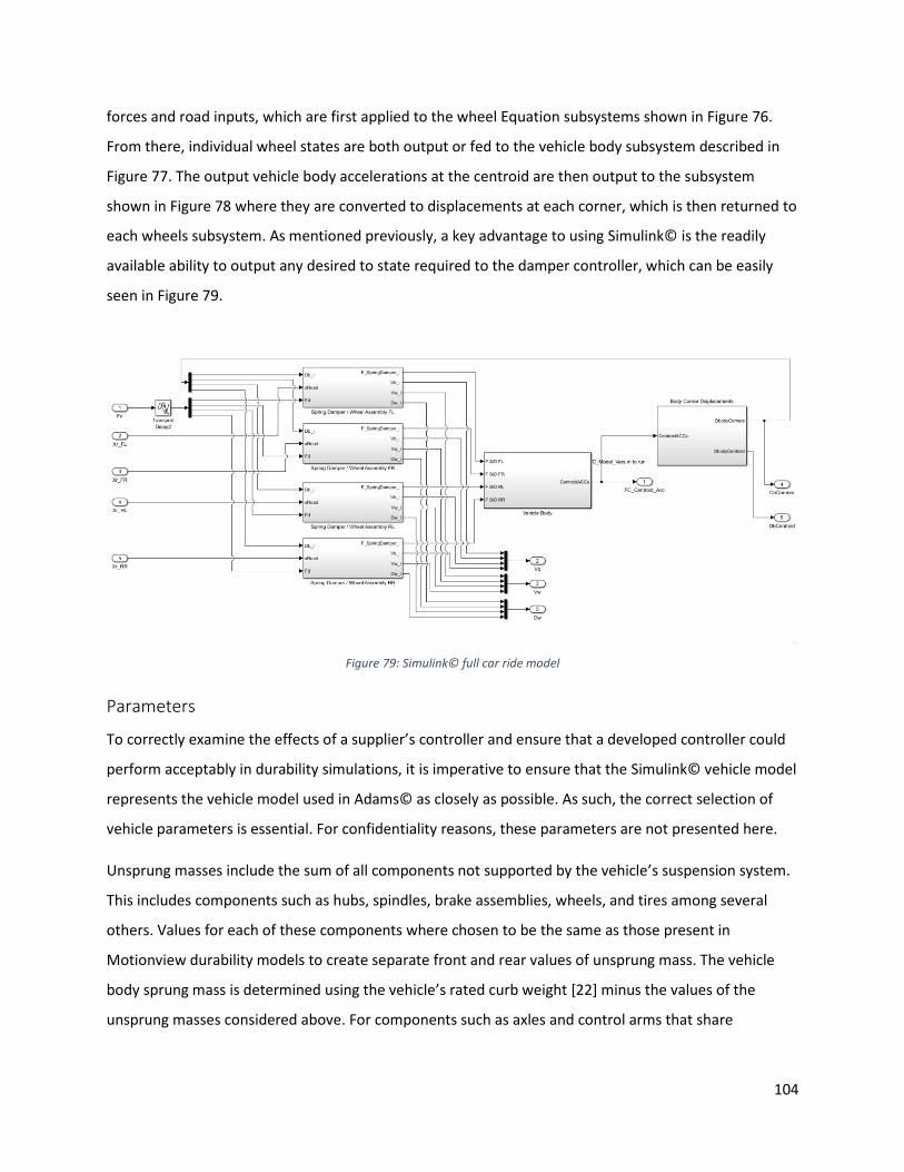
104

forces and road inputs, which are first applied to the wheel Equation subsystems shown in Figure 76.

From there, individual wheel states are both output or fed to the vehicle body subsystem described in

Figure 77. The output vehicle body accelerations at the centroid are then output to the subsystem

shown in Figure 78 where they are converted to displacements at each corner, which is then returned to

each wheels subsystem. As mentioned previously, a key advantage to using Simulink© is the readily

available ability to output any desired to state required to the damper controller, which can be easily

seen in Figure 79.

Figure 79: Simulink© full car ride model

Parameters

To correctly examine the effects of a supplier’s controller and ensure that a developed controller could

perform acceptably in durability simulations, it is imperative to ensure that the Simulink© vehicle model

represents the vehicle model used in Adams© as closely as possible. As such, the correct selection of

vehicle parameters is essential. For confidentiality reasons, these parameters are not presented here.

Unsprung masses include the sum of all components not supported by the vehicle’s suspension system.

This includes components such as hubs, spindles, brake assemblies, wheels, and tires among several

others. Values for each of these components where chosen to be the same as those present in

Motionview durability models to create separate front and rear values of unsprung mass. The vehicle

body sprung mass is determined using the vehicle’s rated curb weight [22] minus the values of the

unsprung masses considered above. For components such as axles and control arms that share

105

attachment points on both sprung and unsprung masses, half of the mass was considered to be part of

the sprung mass, and half part of the unsprung mass.

Values for vehicle dimensions used for track width and to locate the vehicle centroid longitudinally are

taken from published vehicle specifications found in [22].The vehicle body centroid is assumed to be

laterally centered, and the longitudinal position is determined using the published value for front and

rear weight distribution [22].

Springs are assumed to have linear coefficients, the front and rear values of which are equivalent to

those used in durability testing. In addition, the installation ratio between the spring and wheel motion

is considered to ensure that appropriate amount of force acts on the system proportional to its motion.

Therefore, for the purpose of simplicity in this model, linear spring and damping coefficients for the

simple vertical tire model are typical of those found in various published full car ride models [9] [23].

Assumptions, Simplifications and Potential Improvements

Simplifications applied to the Simulink© model for more efficient controller tuning results in

compromises being made in how well the Simulink© model reflects durability models and in turn the

actual chassis.

The most obvious simplification made is the lack of any physical geometry, specifically all suspension

kinematics. The exception being the consideration of the spring and damper installation ratio.

Moreover, on the topic of physical geometry simplifications, it is assumed that the roll and pitch centers

are in the same location as the vehicle centroid. Furthermore, the Simulink© model used for tuning

does not include the effects of anti-roll bars on both the front and rear axles. Emittances having smaller

effects on the accuracy of the model include damper top mounts, bushing effects, or the effects of large

sprung point masses such as the motor, transmission, and occupants.

The above assumptions were deemed necessary to make, as simulation speed is paramount. The

intended use of the Simulink© Full car ride model in optimization algorithms requiring several iterations

to determine controller parameters. The less computationally heavy the quarter car model is allowed to

be, the faster that controller parameters may be optimized.

106

Vita Auctoris

Kyle Hugo was born in 1993 in Calgary, Alberta. He graduated from St. Francis High School in 2011. From

there he went on to the University of Calgary where he obtained a B.Sc. in Mechanical Engineering and

ruined several Formula SAE cars. He is currently a candidate for the MASc. degree in Automotive

Engineering at the University of Windsor and hopes to graduate in Summer 2019.