Virtual lifeeco-evolutionary experiments with situated agents

Walter de BackDepartment of Philosophy

Utrecht University

walter.deback.net

walter@deback.net

Supervisors

Marco Wiering

Intelligent Systems group

Department for Information and Computing Sciences

Edwin de Jong

Large Distributed Databases group

Department for Information and Computing Sciences

Daniel van der Post

Theoretical Biology / Bioinformatics group

Department of Biology

March 2006

2

Abstract

The growing interest in the biological roots of cognition leads to the cross-fertilization between the fields of autonomous robotics and artificial life. Thisrequires new tools that facilitate research on the interface between embod-ied cognitive science and theoretical biology. In this thesis, a model is pre-sented that enables the simulation of evolving ecosystems of situated agents.This model enables studies to the interplay between situated interaction, self-organised collective behaviour and evolution by natural selection.

The use of complex computer simulations as scientific tools requires a the-oretical embedding. This is established by analysing and interpreting the re-sults of ecological simulations (of bitrophic and tritrophic food chains) in termof analytical models of population dynamics. These ordinary differential equa-tion (ODE) models allow us to understand and control the population dynam-ics that emerge from simulations. Moreover, the evolutionary dynamics ob-served in eco-evolutionary simulations can be interpreted as changes in theODE model, which enables us to understand evolvability of certain traits interms of ecological viability.

In this thesis, several eco-evolutionary experiments are replicated that werepreviously conducted by more formal models: predator-prey systems, enrich-ment, tragedy of the commons, evolutionary arms races, red queen effect, evo-lution of reproductive restraint. The simulation model allows us to gain newinsights by relaxing some of the assumptions of these formal models (infinitepopulation sizes, global interactions, spatial homogeneity) and comparing theresults. An indirect explanatory framework is used in which one gives expla-nations of an emergent pattern (e.g. evolutionary dynamics) by relating it toother emergent patterns (population and spatial dynamics), without the needto refer to the specification of the simulation model itself.

The combination of the complex simulation model, its embedding in the-oretical ecology and the use of an indirect explanatory framework, providesa valuable new tool for use in research on the edge of artificial life and au-tonomous robotics, or theoretical biology and embodied cognitive science ingeneral.

Contents

1 Introduction 31.1 Problems . . . . . . . . . . . . . . . . . . . . . . . . . . . . . . . . 41.2 Robotics and artificial life . . . . . . . . . . . . . . . . . . . . . . 41.3 Methodology . . . . . . . . . . . . . . . . . . . . . . . . . . . . . 61.4 Contributions . . . . . . . . . . . . . . . . . . . . . . . . . . . . . 91.5 Outline . . . . . . . . . . . . . . . . . . . . . . . . . . . . . . . . . 11

2 Background 122.1 Embodied situated interaction . . . . . . . . . . . . . . . . . . . . 122.2 Collective behavior . . . . . . . . . . . . . . . . . . . . . . . . . . 142.3 Evolution . . . . . . . . . . . . . . . . . . . . . . . . . . . . . . . . 182.4 Conclusion . . . . . . . . . . . . . . . . . . . . . . . . . . . . . . . 22

3 Simulation model 233.1 Virtual life model . . . . . . . . . . . . . . . . . . . . . . . . . . . 243.2 Emergent patterns . . . . . . . . . . . . . . . . . . . . . . . . . . . 323.3 Conclusions . . . . . . . . . . . . . . . . . . . . . . . . . . . . . . 40

4 Ecological analysis 414.1 Resource and consumer dynamics . . . . . . . . . . . . . . . . . 424.2 Ecological models . . . . . . . . . . . . . . . . . . . . . . . . . . . 454.3 Controlled ecosystem . . . . . . . . . . . . . . . . . . . . . . . . . 534.4 Conclusions . . . . . . . . . . . . . . . . . . . . . . . . . . . . . . 55

5 Evolutionary experiments 565.1 Evolution . . . . . . . . . . . . . . . . . . . . . . . . . . . . . . . . 575.2 Coevolution . . . . . . . . . . . . . . . . . . . . . . . . . . . . . . 625.3 Multi-level selection . . . . . . . . . . . . . . . . . . . . . . . . . 715.4 Conclusions . . . . . . . . . . . . . . . . . . . . . . . . . . . . . . 81

6 Conclusions 846.1 Summary . . . . . . . . . . . . . . . . . . . . . . . . . . . . . . . . 846.2 Discussion . . . . . . . . . . . . . . . . . . . . . . . . . . . . . . . 86

2

Chapter 1

Introduction

The idea that there is a continuity between life and cognition causes a grow-ing interest into the biological origins of cognition. The common denominatorof living and cognitive processes is that they involve self-organization arisingfrom interaction between underlying entities. This perspective has resulted inchanges in cognitive science and artificial intelligence, as well as in theoreticalbiology and ecology, which has caused these fields to grow closer to each other.

This is most clearly demonstrated by cross-fertilization between autonomousrobotics and artificial life. Traditionally, the field of autonomous robotics is con-cerned with the control of an individual embodied situated agent that interactswith its environment. The field of artificial life, instead, traditionally focuses onself-organization of collectives or on population-level evolutionary dynamics.Recently, attention is shifting to research in which the approaches of roboticsand artificial life are combined.

In this thesis, we present the virtual life simulation model that aims to fa-cilitate such research. The simulation implements spatially explicit individual-based models in which individuals are situated agents. The interactions be-tween agents and their environment and among each other give rise to multi-ple self-organised spatial and temporal patterns. Theoretical ecological mod-elling is used to understand the patterns, in ecological and evolutionary con-texts.

After an overview of the scientific embedding of this thesis, in Chapter 1,and its central background concepts, in Chapter 2, the simulation model ispresented in Chapter 3. The population dynamics that arise from these simu-lations are analysed using models from theoretical ecology in Chapter 4. Thetheoretical understanding that results from these models is employed to gaininsight into the results from a series of eco-evolutionary experiments in Chap-ter 5. Finally, conclusions are drawn and opportunities for future research arediscussed in Chapter 6.

3

1.1 Problems

The last two decades have brought the rise of new modelling approaches incognitive science, artificial intelligence and theoretical biology. Instead of mod-elling cognitive behavior in terms of complex internal mechanisms, new em-bodied approaches in cognitive science focus on the situated interaction be-tween relatively simple robotic agents and their environment (Pfeifer and Scheier,1999). Theoretical biology has shown a shift from mathematical mini-models ofecological and evolutionary processes towards individual-based and spatiallyexplicit simulation models in which local interactions among individuals resultin global phenomena (Hutson et al., 1988; Hogeweg and Hesper, 1990; Grimm,1999). These developments have resulted in the rise of autonomous roboticsand artificial life simulations as common modelling tools for these fields.

Whereas autonomous robotics concentrates on the control and interactionof an individual robot with its environment, artificial life simulations typicallyfocus on group- and population-level processes. The field of artificial life canbe divided into studies in either self-organised collective behaviors or evolu-tionary processes. Recently, the interests of robotics and artificial life have agrowing overlap in combinations and interplay of the processes involved inembodied situated interaction, collective behaviors and evolutionary dynam-ics.

In these converging research fields, new simulation models are needed thatfacilitate this research. Moreover, methods of theoretical analysis are necessaryto enable us to interpret the results of these simulations, and embed them inan established theoretical framework. Both these problems are addressed inthis thesis. A simulation model is presented that allows the spatially explicitsimulation of evolving ecosystems of populations of situated individuals. Anda corresponding theoretical model is constructed that is based on well-studiedmodels in ecology.

1.2 Robotics and artificial life

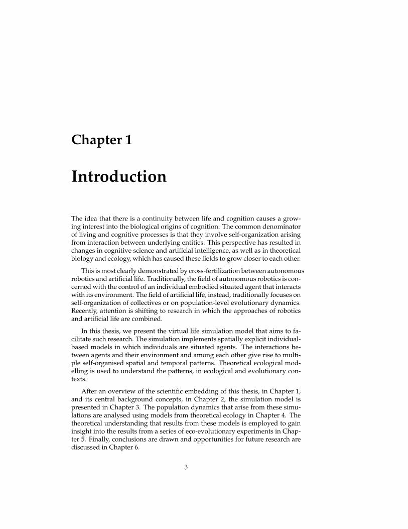
In new approaches to cognitive science and theoretical biology, the concept ofinteraction plays a vital role. In embodied approaches to cognitive science,behavior is re-conceptualised as the result of agent-environment interaction,which has moved the focus from cognition as logical reasoning towards situ-ated interaction. Complexity of behavior is largely a reflection of the richnessof the environment (Simon, 1969; Brooks, 1985) and can result from embod-ied agents (figure 1.1a) with simple control systems (Braitenberg, 1984). In asimilar vein, a-life attempts to explain collective behavioral phenomena suchas bird flocks (figure 1.1b) or coordination in social insects on the basis of self-organization through interactions between groups of relatively simple individ-uals (Reynolds, 1987; Melhuish and Holland, 1999). Evolutionary approachesto behavior have turned from a concept of evolution as an optimization pro-cess towards evolution as adaptation to the problems posed by the ecology.

4

Figure 1.1: (Left) Khepera robot: used in evolutionary robotics (Nolfi and Flo-reano, 2000). (Middle) BOIDS model: example of collective a-life (Reynolds,1987). (Right) Self-structured spiral waves in cellular automata model of evo-lution (Savill and Hogeweg, 1997)

This is reflected in a shift from exogenous fitness models in which selection isimposed externally by user-defined fitness functions towards endogenous fit-ness models (figure 1.1c) (Forrest and Mitchell, 1994; Ray, 1991; Menczer andBelew, 1996). In such models the fitness of individuals, defined as the rate ofreproduction, results from interactions within the system (e.g. survival andreproduction).

The processes of embodied situated interaction, collective behavior andevolution by natural selection models have already been studied extensivelyas isolated mechanisms (see chapter 2). More recently, interest in combinationsof these processes is increasing. In autonomous robotics, the potential of self-organization in collective behaviors and evolutionary design is acknowledged.And in theoretical biology, modern modelling approaches use individual-basedand spatially explicit simulation that yield radically different dynamics thanpredicted by classical population-level models.

Swarm robotics, for example, combines the first two topics in studyingcollective phenomena that emerge from physically situated robots (Bonabeauet al., 1999). Evolutionary robotics combines robotics with evolutionary opti-mization, and recently attention has shifted towards less explicit fitness criteria(e.g. through applying coevolution) (Harvey et al., 1997; Nolfi and Floreano,2000). In theoretical biology renewed attention is given to the controversialtheme of group selection which combines self-organised collectives with evo-lutionary mechanisms by holding that such collectives can serve as a unit of se-lection and thus influence the course of evolution (Wilson, 1975; Johnson andBoerlijst, 2002; Savill and Hogeweg, 1997). Other studies combine embodiedsituated interaction with endogenous fitness models by evolving (simulated)robots through natural selection (Yaeger, 1994; Channon, 2000).

Attempts to study the combination and interplay of situated interactionwith ecological and evolutionary processes have been rare, however. Thisthesis constitutes a modest first step towards this end. The present study isfocused on simulation and theoretical understanding of ecological and evolu-tionary phenomena that arise from interacting situated agents.

5

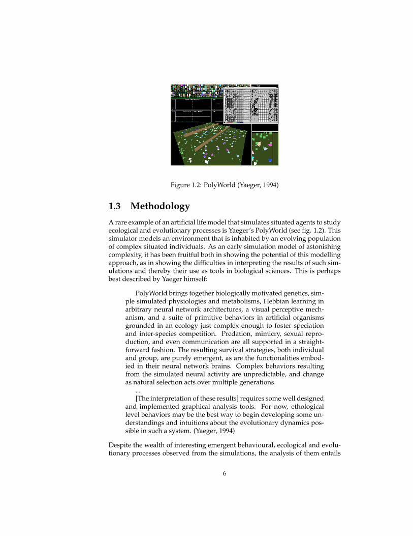
Figure 1.2: PolyWorld (Yaeger, 1994)

1.3 Methodology

A rare example of an artificial life model that simulates situated agents to studyecological and evolutionary processes is Yaeger’s PolyWorld (see fig. 1.2). Thissimulator models an environment that is inhabited by an evolving populationof complex situated individuals. As an early simulation model of astonishingcomplexity, it has been fruitful both in showing the potential of this modellingapproach, as in showing the difficulties in interpreting the results of such sim-ulations and thereby their use as tools in biological sciences. This is perhapsbest described by Yaeger himself:

PolyWorld brings together biologically motivated genetics, sim-ple simulated physiologies and metabolisms, Hebbian learning inarbitrary neural network architectures, a visual perceptive mech-anism, and a suite of primitive behaviors in artificial organismsgrounded in an ecology just complex enough to foster speciationand inter-species competition. Predation, mimicry, sexual repro-duction, and even communication are all supported in a straight-forward fashion. The resulting survival strategies, both individualand group, are purely emergent, as are the functionalities embod-ied in their neural network brains. Complex behaviors resultingfrom the simulated neural activity are unpredictable, and changeas natural selection acts over multiple generations.

...[The interpretation of these results] requires some well designed

and implemented graphical analysis tools. For now, ethologicallevel behaviors may be the best way to begin developing some un-derstandings and intuitions about the evolutionary dynamics pos-sible in such a system. (Yaeger, 1994)

Despite the wealth of interesting emergent behavioural, ecological and evolu-tionary processes observed from the simulations, the analysis of them entails

6

little more than anthropomorphic description of observed behaviours. It is un-clear how the labelling of observed behaviours with exotic names like ’freneticjoggers’ and ’indolent cannibals’ contributes to a deeper understanding of thesimulation results or biological science in general. Indeed, the benefits of sim-ulation models are lost when the results are almost as hard to analyse as thereal world.

This is not necessarily the case for complex artificial life simulations, asthis thesis attempts to point out. There is, however, a need for a theoreticalembedding in the initial construction of the model to be able to interpret theresults of simulations in a later stage. A theoretical understanding has been anintegral part of the development of the virtual life simulation model. This startsfrom a general perspective on the use of computer simulations in scientificinquiry.

Simulation as scientific tools1

Computer simulations are among the most flexible and powerful new tools fortheoretical development in biology. This does not imply, however, that theyare necessarily easier to understand or more useful than other tools such aspurely mathematical models. Although it is relatively easy to construct com-puter models that simulate complex situations that go beyond mathematicaltractability, this can be a disadvantage with respect to scientific inquiry aimedat understanding biological processes. When simulations are too complex ortoo different from existing (mathematical) models, their scientific value is hardto assess since they defy comparison to existing biological theory.

A fruitful way of incorporating simulations into scientific activity is to con-sider them as ordinary tools (like hammers or microscopes) that are constructedto overcome our bodily shortcomings. Scientific activity can be seen as a cog-nitive form of skillful activity aimed at gaining a maximal grip on the environ-ment in which we find ourselves (Merleau-Ponty, 1943; Dreyfus). A tool, orrather the use of a tool, serves as a corporeal enhancement by elaborating onthe range of skillful activities of the user. The use of a microscope, for exam-ple, extends our visual abilities to discriminate between very small objects. Itsuse only becomes meaningful to the user when he can embed this particularform of visual experiences in the frameworks of embodied skills he is alreadyfamiliar with through a process of skill acquisition.

Similarly, the use of computer simulations becomes meaningful and usefulonly relative to the degree of integration into existing theoretical frameworks.The value of a new scientific tool can only be assessed if it allows comparison tocommon norms. For the introduction of new simulation tools to be successful,the new tool should be accompanied by a body of theory that validates itsuse. This does not mean that simulations do not present genuine new toolsmerely because they are validated by existing theory. New tools can open new

1The following two paragraphs are roughly based on the excellent overview of methodologicalissues by di Paolo (1999, ch 4).

7

grounds for research by (re)moving parts of the old web of constraints (as isillustrated by the development of cell biology following the invention of themicroscope by Antonius van Leeuwenhoek).

The advantages of computer simulations lie mainly in the fact that they en-able exploration of the emergent properties from local individual interactions.This renders simulation models new and potentially very useful. Within thedomain of biology, the study of the emergence of new levels of organizations(e.g. cells, individuals, societies) and the interactions between the dynamicsof the various levels is essential. New theoretical modelling shows that manytraditional distinctions are not as clear-cut as they were supposed to be. Incontrast to the habit of separating ecological and evolutionary timescale, forexample, new eco-evolutionary models in which this simplification was liftedshow that the interplay between these dynamics have strong influences on eachother.

Direct and indirect explanation

A large part of research in artificial life is conducted to show and understandthe emergence of complex global dynamics from simple local interactions. Thepower of self-organization has been demonstrated in early work such as thesimulation of bird flocking by Reynolds (1987). Reynold’s model (see figure1.1) acted as a proof of concept by showing that a complex phenomenon suchas coordinated collective behaviour can be reproduced by invoking three sim-ple local rules between interacting individuals. This way of using computersimulations has been fruitful to gain recognition for self-organization as animportant property of biological systems, which has since become widely ac-cepted. What is also increasingly recognized, however, is the limitation of thisapproach, because it proceeds on the conjecture that the ability to replicate acertain phenomenon does not imply understanding of how the pattern arisesfrom the model. In many cases, it may be difficult or even impossible to pre-cisely know what aspects of the model are involved and how they relate. Inany case, the explanation of the observed pattern is done by relating the phe-nomena to the simulation model directly (see left panel in figure 1.3). This isonly one, rather limited, approach to the use of simulation models in biology.

A much more interesting and powerful way of using computer simulationsis in applying an indirect way of explanation. Artificial life simulation modelsoften give rise to multiple emergent patterns simultaneously2. Some of theseobservations can be explained by the basic model itself, but others may requireto be explained in terms of other emergent patterns (see right panel in figure1.3).

The present study attempts to provide insight into (1) ecological dynamics(e.g. population dynamics and spatial self-organization) by relating them tothe local interacting agents and (2) evolutionary dynamics (e.g. coevolution-ary arms races and group selection) by relating them to ecological dynamics.

2This depends, of course, on the number of free parameters in the model and the choise ofobservables that show the patterns.

8

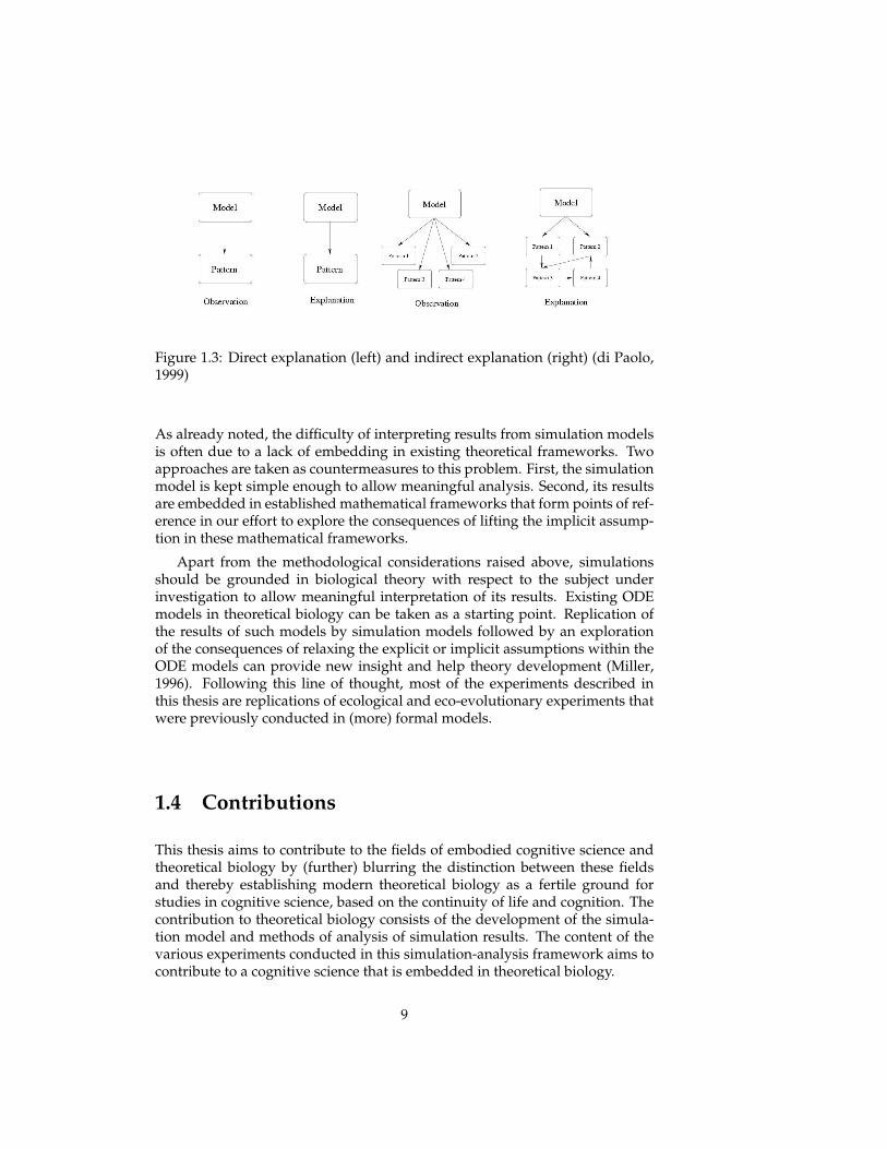
Figure 1.3: Direct explanation (left) and indirect explanation (right) (di Paolo,1999)

As already noted, the difficulty of interpreting results from simulation modelsis often due to a lack of embedding in existing theoretical frameworks. Twoapproaches are taken as countermeasures to this problem. First, the simulationmodel is kept simple enough to allow meaningful analysis. Second, its resultsare embedded in established mathematical frameworks that form points of ref-erence in our effort to explore the consequences of lifting the implicit assump-tion in these mathematical frameworks.

Apart from the methodological considerations raised above, simulationsshould be grounded in biological theory with respect to the subject underinvestigation to allow meaningful interpretation of its results. Existing ODEmodels in theoretical biology can be taken as a starting point. Replication ofthe results of such models by simulation models followed by an explorationof the consequences of relaxing the explicit or implicit assumptions within theODE models can provide new insight and help theory development (Miller,1996). Following this line of thought, most of the experiments described inthis thesis are replications of ecological and eco-evolutionary experiments thatwere previously conducted in (more) formal models.

1.4 Contributions

This thesis aims to contribute to the fields of embodied cognitive science andtheoretical biology by (further) blurring the distinction between these fieldsand thereby establishing modern theoretical biology as a fertile ground forstudies in cognitive science, based on the continuity of life and cognition. Thecontribution to theoretical biology consists of the development of the simula-tion model and methods of analysis of simulation results. The content of thevarious experiments conducted in this simulation-analysis framework aims tocontribute to a cognitive science that is embedded in theoretical biology.

9

1.4.1 Contributions to Artificial Life

Development of simulation platform

A simulation model is developed that facilitates the study of the interplay be-tween situated interaction, self-organization and evolution by natural selec-tion. The result is a spatially-explicit individual-based model in which ecolog-ical and evolutionary processes are simulated. Like most artificial life simu-lations, the model is defined on the level of (situated) individuals, while ourmain interest is at the level of (evolving) populations. Although individualsare modelled as simple agents throughout this thesis to keep results analyti-cally tractable, the model is easily extended to more complex morphologies,more elaborate (neural) control systems and more complex agent-agent inter-actions (e.g. signalling).

Development of methodology for theoretical analysis and interpretation

To render the results of these simulations useful for scientific enquiry, the re-sults are interpreted in the well-established framework of theoretical ecology.Analytical ODE models enable us to predict, manipulate and control the pop-ulation dynamics that emerge from the simulations. Moreover, they enable usto understand the ecological constraints on evolvability.

Most work in artificial life is restricted to a ’simple to complex’ paradigmand shows that simple local interactions lead to the complex global patterns byemploying a direct explanation model. The simulations presented in this thesisare an attempt to transcend this paradigm towards the ’complex to complex’by employing indirect explanations, in which the emergence of one pattern isexplained in terms of its relations to other emergent patterns. This explana-tory strategy renders explanations more generic because they depend less onimplementation details of the simulation model. It can therefore be consid-ered a contribution to the use of computer simulations in scientific research ingeneral.

1.4.2 Contributions to Cognitive Artificial Intelligence (CAI)

Although (the evolution of) cognition is not explicitly studied in this thesis, theeco-evolutionary simulations presented here are relevant to cognitive sciencebecause they examine the biological processes in ecology and evolution thatunderly the emergence of cognitive behaviour.

Cognition is an adaptation to ecological problems

From an evolutionary perspective, cognition is considered as an adaptation toproblems posed by the demands of the ecology. The complexity of behaviouris related to the complexity of the environment, as Rössler (1974) pointed out.Even a random walk is sufficient for survival and reproduction if food is abun-dant in a given environment. If food are distributed more spaciously, more

10

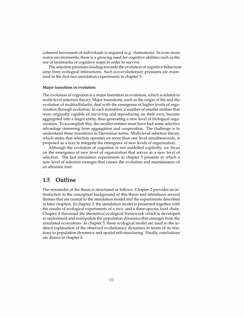
coherent movement of individuals is required (e.g. chemotaxis). In even morescarce environments, there is a growing need for cognitive abilities such as theuse of landmarks or cognitive maps in order to survive.

The selection pressures leading towards the evolution of cognitive behaviourarise from ecological interactions. Such eco-evolutionary pressures are exam-ined in the first two simulation experiments in chapter 5.

Major transition in evolution

The evolution of cognition is a major transition in evolution, which is related tomulti-level selection theory. Major transitions, such as the origin of life and theevolution of multicellularity, deal with the emergence of higher levels of orga-nization through evolution. In each transition, a number of smaller entities thatwere originally capable of surviving and reproducing on their own, becameaggregated into a larger entity, thus generating a new level of biological orga-nization. To accomplish this, the smaller entities must have had some selectiveadvantage stemming from aggregation and cooperation. The challenge is tounderstand these transitions in Darwinian terms. Multi-level selection theory,which states that selection operates on more than one level simultaneously, isproposed as a way to integrate the emergence of new levels of organization.

Although the evolution of cognition is not modelled explicitly, we focuson the emergence of new level of organization that serves as a new level ofselection. The last simulation experiments in chapter 5 presents in which anew level of selection emerges that causes the evolution and maintainance ofan altruistic trait.

1.5 Outline

The remainder of the thesis is structured as follows. Chapter 2 provides an in-troduction to the conceptual background of this thesis and introduces severalthemes that are central to the simulation model and the experiments describedin later chapters. In chapter 3, the simulation model is presented together withthe results of ecological experiments of a two- and a three-species food chain.Chapter 4 discussed the theoretical ecological framework which is developedto understand and manipulate the population dynamics that emerges from thesimulated ecosystems. In chapter 5, these ecological model are used in the in-direct explanation of the observed evolutionary dynamics in terms of its rela-tions to population dynamics and spatial self-structuring. Finally, conclusionsare drawn in chapter 6.

11

Chapter 2

Background

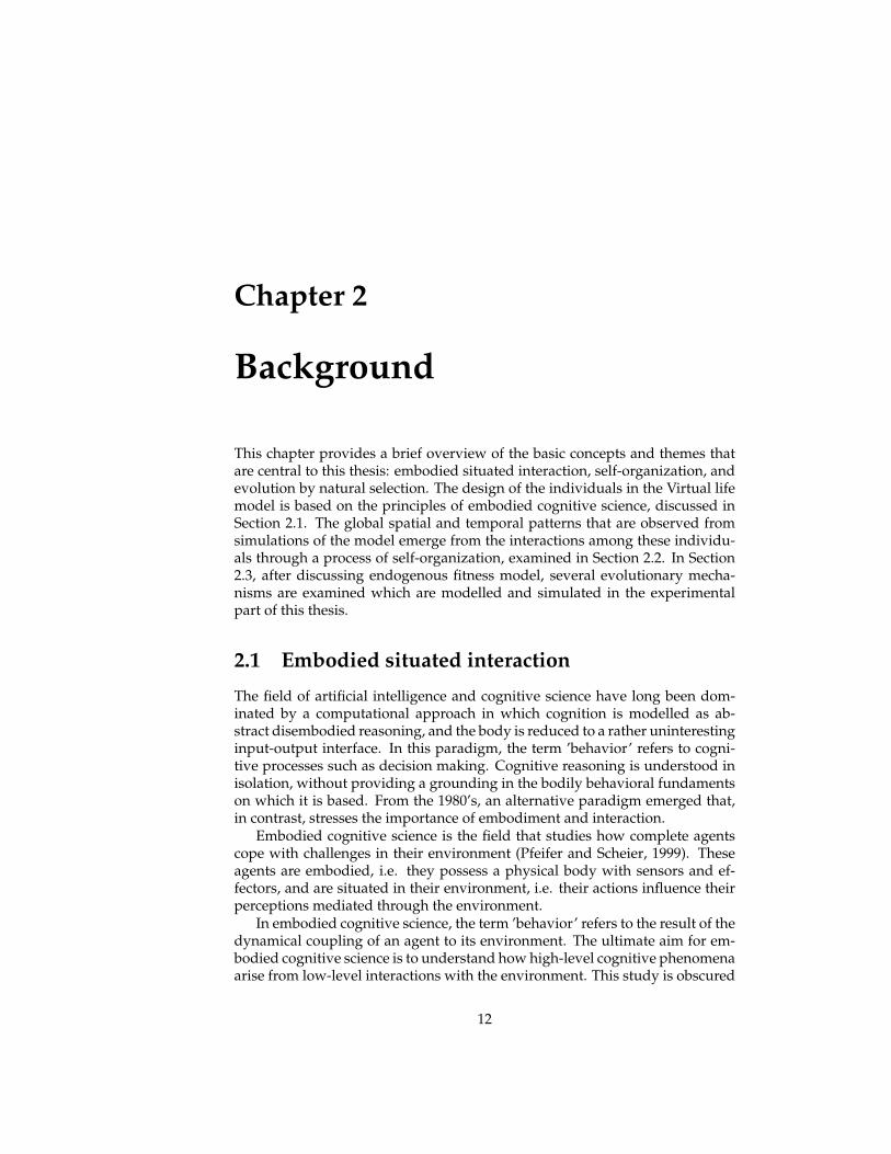
This chapter provides a brief overview of the basic concepts and themes thatare central to this thesis: embodied situated interaction, self-organization, andevolution by natural selection. The design of the individuals in the Virtual lifemodel is based on the principles of embodied cognitive science, discussed inSection 2.1. The global spatial and temporal patterns that are observed fromsimulations of the model emerge from the interactions among these individu-als through a process of self-organization, examined in Section 2.2. In Section2.3, after discussing endogenous fitness model, several evolutionary mecha-nisms are examined which are modelled and simulated in the experimentalpart of this thesis.

2.1 Embodied situated interaction

The field of artificial intelligence and cognitive science have long been dom-inated by a computational approach in which cognition is modelled as ab-stract disembodied reasoning, and the body is reduced to a rather uninterestinginput-output interface. In this paradigm, the term ’behavior’ refers to cogni-tive processes such as decision making. Cognitive reasoning is understood inisolation, without providing a grounding in the bodily behavioral fundamentson which it is based. From the 1980’s, an alternative paradigm emerged that,in contrast, stresses the importance of embodiment and interaction.

Embodied cognitive science is the field that studies how complete agentscope with challenges in their environment (Pfeifer and Scheier, 1999). Theseagents are embodied, i.e. they possess a physical body with sensors and ef-fectors, and are situated in their environment, i.e. their actions influence theirperceptions mediated through the environment.

In embodied cognitive science, the term ’behavior’ refers to the result of thedynamical coupling of an agent to its environment. The ultimate aim for em-bodied cognitive science is to understand how high-level cognitive phenomenaarise from low-level interactions with the environment. This study is obscured

12

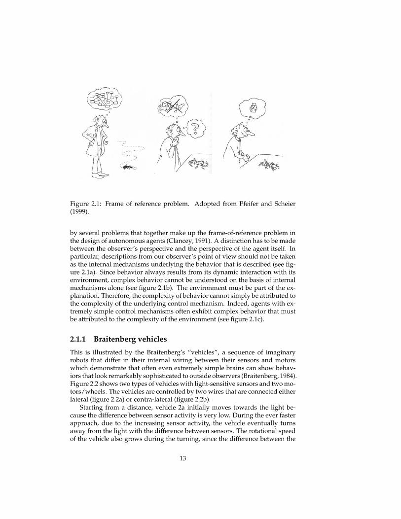
Figure 2.1: Frame of reference problem. Adopted from Pfeifer and Scheier(1999).

by several problems that together make up the frame-of-reference problem inthe design of autonomous agents (Clancey, 1991). A distinction has to be madebetween the observer’s perspective and the perspective of the agent itself. Inparticular, descriptions from our observer’s point of view should not be takenas the internal mechanisms underlying the behavior that is described (see fig-ure 2.1a). Since behavior always results from its dynamic interaction with itsenvironment, complex behavior cannot be understood on the basis of internalmechanisms alone (see figure 2.1b). The environment must be part of the ex-planation. Therefore, the complexity of behavior cannot simply be attributed tothe complexity of the underlying control mechanism. Indeed, agents with ex-tremely simple control mechanisms often exhibit complex behavior that mustbe attributed to the complexity of the environment (see figure 2.1c).

2.1.1 Braitenberg vehicles

This is illustrated by the Braitenberg’s “vehicles”, a sequence of imaginaryrobots that differ in their internal wiring between their sensors and motorswhich demonstrate that often even extremely simple brains can show behav-iors that look remarkably sophisticated to outside observers (Braitenberg, 1984).Figure 2.2 shows two types of vehicles with light-sensitive sensors and two mo-tors/wheels. The vehicles are controlled by two wires that are connected eitherlateral (figure 2.2a) or contra-lateral (figure 2.2b).

Starting from a distance, vehicle 2a initially moves towards the light be-cause the difference between sensor activity is very low. During the ever fasterapproach, due to the increasing sensor activity, the vehicle eventually turnsaway from the light with the difference between sensors. The rotational speedof the vehicle also grows during the turning, since the difference between the

13

Figure 2.2: Braitenberg vehicles. Adopted From(Braitenberg, 1984).

sensors increases through turning. Vehicle 2b also approaches the light at anincreasing speed. This vehicle does however not avoid the light, but instead itsteers towards the source and hit it at top speed, possibly destroying the lightbulb.

External observers, lacking knowledge of the internal mechanisms, mightcharacterize these behavior as either timid or aggressive, and give explanationsbased on mental states such as beliefs, desires and intentions. Such observer-side ascriptions of behavior are characteristic of traditional cognitive scienceand artificial intelligence. Embodied cognitive science and artificial life, in-stead, attempt to understand behavior in terms of situated sensorimotor activ-ity involved in agent-environment interaction.

2.2 Collective behavior

The environment with which animals interact typically includes other animals.Local interactions between agents, as a subset of agent-environment interac-tions, can result in the spontaneous formation of novel behavioral patterns ona global scale, as a result of a process of self-organization.

2.2.1 Self-organization

Self-organization is ubiquitous in nature. In many scientific domains, varyingfrom physics and chemistry, to biology and economics, models have been de-veloped that show that simple interaction between many system componentsat the local level may lead to (often unexpected) complex phenomena at theglobal level. This spontaneous emergence of global phenomena has led to in-triguing new insights, since it shows that complex patterns need not be guidedby central control, nor predesigned in the behavioural rules of its components.

14

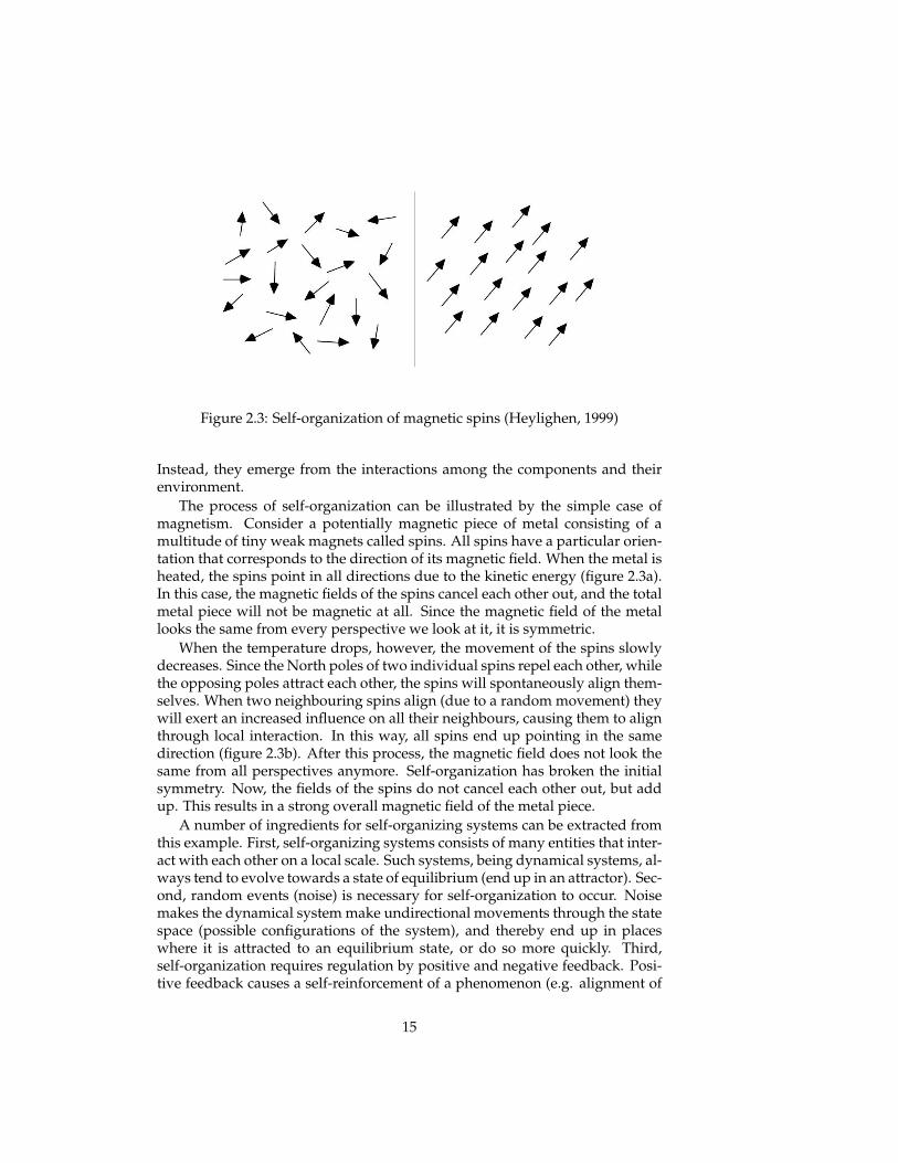
Figure 2.3: Self-organization of magnetic spins (Heylighen, 1999)

Instead, they emerge from the interactions among the components and theirenvironment.

The process of self-organization can be illustrated by the simple case ofmagnetism. Consider a potentially magnetic piece of metal consisting of amultitude of tiny weak magnets called spins. All spins have a particular orien-tation that corresponds to the direction of its magnetic field. When the metal isheated, the spins point in all directions due to the kinetic energy (figure 2.3a).In this case, the magnetic fields of the spins cancel each other out, and the totalmetal piece will not be magnetic at all. Since the magnetic field of the metallooks the same from every perspective we look at it, it is symmetric.

When the temperature drops, however, the movement of the spins slowlydecreases. Since the North poles of two individual spins repel each other, whilethe opposing poles attract each other, the spins will spontaneously align them-selves. When two neighbouring spins align (due to a random movement) theywill exert an increased influence on all their neighbours, causing them to alignthrough local interaction. In this way, all spins end up pointing in the samedirection (figure 2.3b). After this process, the magnetic field does not look thesame from all perspectives anymore. Self-organization has broken the initialsymmetry. Now, the fields of the spins do not cancel each other out, but addup. This results in a strong overall magnetic field of the metal piece.

A number of ingredients for self-organizing systems can be extracted fromthis example. First, self-organizing systems consists of many entities that inter-act with each other on a local scale. Such systems, being dynamical systems, al-ways tend to evolve towards a state of equilibrium (end up in an attractor). Sec-ond, random events (noise) is necessary for self-organization to occur. Noisemakes the dynamical system make undirectional movements through the statespace (possible configurations of the system), and thereby end up in placeswhere it is attracted to an equilibrium state, or do so more quickly. Third,self-organization requires regulation by positive and negative feedback. Posi-tive feedback causes a self-reinforcement of a phenomenon (e.g. alignment of

15

spins) which ends when all components are absorbed by a new system config-uration, leaving the system in a stable negative feedback state.

It has been argued that actually most dynamical systems can be said to beself-organizing in one way or the other, depending on the way and level ofdescription. Self-organization is thus a way of modelling systems, rather thana class of systems. A system becomes describable as a self-organizing systemwhen the level of description is being pitched on a lower level (Gershenson andHeylighen, 2003). If, for example, we describe the brain in relation to the bodilyfunctions, it serves as a central control unit. When the level of description ismoved to the neuronal level, however, the function of the brain is describablea self-organised system.

The perspective of self-organizing system nevertheless remains essential inthe field of artificial life modelling since explanations of emergence, evolution,and development of the life and behavior of living systems cannot be given byrestricting models to a single level of organization or abstraction (Gershensonand Heylighen, 2003).

2.2.2 Biological systems

Self-organized processes are very common in biological systems. The mech-anisms of self-organization in biological systems differ from physical systemsin an important way: The interacting entities are usually much more complex.Whereas physical systems are composed of magnetic spins or grains of sand,the components of biological systems are neurons, ants or birds (Camazineet al., 2001).

As a result of this, the interaction between entities is typically far more elab-orate than in physical systems. The interaction is not limited to physical lawsas magnetism of gravity, but often show rich patterns of behavioral interac-tions. Moreover, insofar as these behavioral rules are genetically specified, aninteresting dimension to collective behavior is added, because natural selectioncan adapt the rules of interaction, and thereby shaping the collective behaviorsthat can be formed (Camazine et al., 2001).

Many collective behaviors in biological systems can be understood as re-sulting from self-organization. Social insect behaviors are the primary sourceof inspiration for theories of collective behavior, but they are also applied tobirds, primates and human beings (e.g. crowding in emergency situations)(Couzin and Krause, 2003). Not all collective behavior is due to self-organization,however. This is only the case where this group behavior is constituted by lo-cal interaction between individuals, independent of global or external control.Some counterexamples are regulation by queens in colonies of social insects orcollective migration of birds in the direction of the sun.

Stigmergy

An interesting mechanism by which biological systems are capable of collec-tive behavior is stigmergy, an indirect form of communication. By interacting

16

with the environment, an individual can change this environment. This caninfluence the behavior of other individuals to form collective phenomena.

Grasse (1959) found that the construction work done by a termite in a par-ticular location changes the sensory input of the termite which in turn altersits behavior, and that of other individuals visiting this location. In this way,the building of termite hills is (spatially) coordinated by the environmentalchanges the work itself induces. Later, it was found that the emission of pheromonesalso played a significant role in the (temporal coordination of the) constructionprocess. Both coordinational processes are completely distributed.

Melhuish and Holland (1999) distinguish between active and passive stig-mergy. Active stigmergy changes the behavior of other individuals in a quali-tative (do something else) or quantitative (do something more frequently) way.Passive stigmergy, on the other hand, does not influence the individual activityin any way (not qualitatively nor quantitatively), but does affect the outcome ofa behavior. This source of self-organization in biological systems is probablythe simplest and most basic form of coordinated action, since it requires theleast behavioral complexity of its participants.

Didabots

Maris and te Boekhorst (1996) have used passive stigmergy, which they call a’strategy of errors’ (Deneubourg et al., 1983), with simple robotic models. Theyused robots, Didabots, with Braitenberg-like control systems1. They have prox-imity sensors making them turn away from close obstacles and walls. Theirenvironment consists of a rectangular area in which boxes are randomly dis-tributed (figure 2.4a). When one of the robot’s proximity sensors is activatedbecause it detects an obstacle, the robot turns away from it. However, the mor-phology of the robots is chosen such that the sensors are in front but are di-rected outward. Therefore, a robot does not detect a box when it collides withit head-on (e.g. see left robot in figure 2.4a). This behavioral error causes arobot to push the box until it detects another box and turns away while leavingthe box it was pushing. The result of this is that there are now two boxes wherepreviously there was only one.

This change in the environment does not influence the behavior of otherindividuals in a qualitative or quantitative way. The robots keep doing theonly thing they can. However, due to the physical changes that were made thechances increase that a third box is left at this location, since two boxes havemore chance than one to be actually detected by the robots. The result of thisauto-catalytic process is the formation of a cluster of boxes. For emergence toa single cluster to occur, it is necessary to use more than one robot to generatethe crucial ’mistakes’ in the obstacle avoidance behavior of the robots. Hereand indeed in many collective behavioral phenomena the frame-of-referenceproblem arises again, since this behavior may be described from an observer’s

1A difference with Braitenberg’s vehicles is that the Didabots also move in the absence of sensoractivation.

17

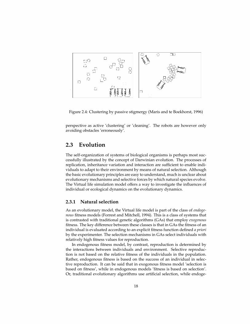
Figure 2.4: Clustering by passive stigmergy (Maris and te Boekhorst, 1996)

perspective as active ’clustering’ or ’cleaning’. The robots are however onlyavoiding obstacles ’erroneously’.

2.3 Evolution

The self-organization of systems of biological organisms is perhaps most suc-cessfully illustrated by the concept of Darwinian evolution. The processes ofreplication, inheritance variation and interaction are sufficient to enable indi-viduals to adapt to their environment by means of natural selection. Althoughthe basic evolutionary principles are easy to understand, much is unclear aboutevolutionary mechanisms and selective forces by which natural species evolve.The Virtual life simulation model offers a way to investigate the influences ofindividual or ecological dynamics on the evolutionary dynamics.

2.3.1 Natural selection

As an evolutionary model, the Virtual life model is part of the class of endoge-nous fitness models (Forrest and Mitchell, 1994). This is a class of systems thatis contrasted with traditional genetic algorithms (GAs) that employ exogenousfitness. The key difference between these classes is that in GAs the fitness of anindividual is evaluated according to an explicit fitness function defined a prioriby the experimenter. The selection mechanisms in GAs select individuals withrelatively high fitness values for reproduction.

In endogenous fitness model, by contrast, reproduction is determined bythe interactions between individuals and environment. Selective reproduc-tion is not based on the relative fitness of the individuals in the population.Rather, endogenous fitness is based on the success of an individual in selec-tive reproduction. It can be said that in exogonous fitness model ’selection isbased on fitness’, while in endogenous models ’fitness is based on selection’.Or, traditional evolutionary algorithms use artificial selection, while endoge-

18

nous fitness models employ natural selection. The former model evolutionaryoptimization and the latter model evolutionary adaptation (Menczer and Belew,1996).

Evolutionary adaptation by differential reproduction can only operate whenthere is variation among individuals. Without variation in the population (i.e.when all individuals are identical), natural selection does not change trait fre-quencies in populations, but it does result in changes in population sizes overtime through reproduction and mortality processes. Endogenous fitness mod-els without variation among individuals define non-evolving ecosystems (dis-cussed in chapters 3 and 4). When variation among individuals is included in atrait that affects reproduction, we obtain eco-evolutionary systems (discussedin chapter 5).

In general, evolutionary change of a population can be attributed to eithernatural selection and genetic drift. The latter occurs when the evolvable traitdoes not affect differential reproduction. In this case, the genetic changes arebasically a stochastic process that arises from the fact that mutations occur intraits that affect fitness. Genetic drift is observed most strongly in small evolv-ing populations. Since the population in the simulation model presented in thenext chapter are rather small, genetic drift must be ruled out in order to iden-tify genuine selection. In the experiments presented in this thesis, this is doneby choosing the evolving trait such that they directly affect fitness.

Selection cannot be based on explicit fitness criteria since these are absentin endogenous fitness models. Instead, it arises through competition amongindividuals for limited resources. This is true for trophic interactions (in foodchains) between populations, but also between individuals of the same pop-ulation. Thus, the fitness of an individual always strongly depends on otherindividuals.

Darwin was well aware of this interdependency: “the structure of everyorganic being is related, in the most essential yet often hidden manner, to thatof all the other organic beings, with which it comes into competition for foodand residence, or from which it has to escape, or on which it preys” (Darwin,1859). In the struggle for energy and reproductive resource, all individuals areenemies of each other, even within a single species. This drives adaptationof the population as a whole through the evolutionary changes that arise inresponse to changes of other members of the population competing for thesame limited resources.

2.3.2 Coevolution

The same evolutionary principle, both sides of interactions driving adaptation,holds for interactions between different populations or species, called coevolu-tion. Coevolution is the mutual evolutionary influence between populations inwhich all populations exert selective pressures on others. The classic exampleis coevolution in predators and prey species which can lead to evolutionaryarms races that can exhibit the red queen effect.

19

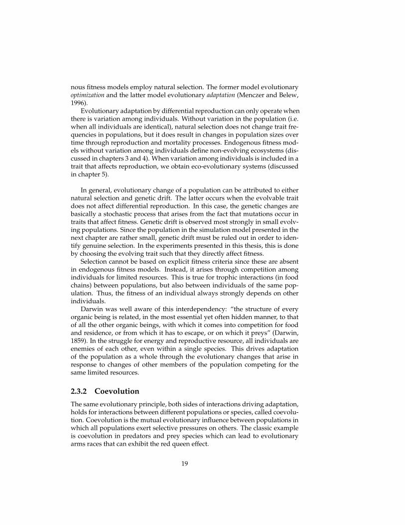
Figure 2.5: Red queen: “In this place, it takes all the running you can do to stay inthe same place.”

Arms races

Foxes and rabbits are involved in a competitive race in two senses. The indi-vidual fox and it rabbit prey are competing on a behavioural time scale in thesame sense as a submarine tries to sink a ship. But on a historical time scale, thedesigners of the submarine may learn from earlier mistakes, and as technologyprogresses, become better at sinking ships. Likewise, the fox population mayevolve improvements for catching rabbits over evolutionary time. In responseto this, the rabbit population may evolve adaptations to outwit the foxes. Bi-ologists refer to such ongoing evolutionary mutual counter-adaptations as anevolutionary ’arms race’ (Dawkins and Krebs, 1979).

Red queen effect

The adaptations obtained in an arms race do, however, not necessarily lead toan improved fitness in the sense of being better adapted to the environment,since this environment evolves as well. van Valen (1973), who studied the ex-tinction rates within and between taxa, noticed that species with longer evolu-tionary histories need not be better adapted to their environment than ’young’species. He proposed the red queen hypothesis to point out that in evolution,populations must continuously adapt to maintain the same level of fitness (seefigure 2.5). In this situation, both species adapt to the other, without either onebecoming more efficient.

2.3.3 Multi-level selection

Darwinian evolutionary theory seems to predict that individuals will alwaysact to increase their own fitness. For this reason, the evolution of altruism(acting to increase the fitness of another individual at the expense of its own)has long been a benchmark problem in evolutionary biology. Not only is itan important issue for understanding altruistic behavior of biological systemsalive today, but also to explain the emergence of new levels of organization,since these major transitions in evolution often require the (partially) releaveof self-interest for the sake of the group (Maynard-Smith and Szathmary, 1995).

20

A first proposal to resolve this problem was the idea that traits can spreadthrough a population because of the benefits they have for groups of individu-als, regardless of the fitness of individuals within that group (Wynne-Edwards,1962, 1963), was heavily criticized on the theoretical grounds that large pop-ulation of altruist individuals would be very susceptible to invasion by self-ish individual and therefore not constitute a stable evolutionary mechanism(Williams, 1966). The latter author developed a concept of the gene as the fun-damental unit of selection, which has become a grand theme in biology, espe-cially following the popularization of the idea of the ’selfish gene’ by Dawkins(1976). The unit of selection was moved down (to a level lower than the indi-vidual) instead of up (to a level higher than the individual).

Group selection was even more pressured by two influential theories inthe 60’s and 70’s. Inclusive fitness theory (a.k.a. kin selection) developed byHamilton (1964) explained how altruism can evolve among genetic relatives,since it pays off in terms of gene propagation to behave altruistically towardskin since relatives carry copies of the genes. Even if one sacrifices himself forclose relatives, the genetic material is preserved for reproduction in anotherindividual. This has greatly contributed to the understanding of altruism inspecies using haplodiploidy (e.g. eusocial communities such as ant colonies).Game-theoretical accounts of the evolution of altruism showed that such be-havior can also evolve among non-relatives if they participate in reciprocal al-truism in Tit-for-Tat situations (Axelrod and Hamilton, 1981).

More recently, however, the concept of group or multi-level selection wasreintroduced by D.S. Wilson et al. (Wilson, 1975; Wilson and Sober, 1994). Theystate that groups of individuals can have functional organisations in the sameway as individuals do and can thereby act as a ’vehicle’ for selection. Thishigher level of selection influences the course of evolution since selection be-tween groups can be in another direction then selection within groups.

Spatially explicit individual-based models are used to emphasise the influ-ence of spatial instead of the genetic relatedness between members of groups (asspiral waves, patches or clusters)2. It is argued that Hamilton’s relatedness isthen not merely the genetical correlation, but depends of local interactions andpopulation dynamics of viscous populations3 (van Baalen and Rand, 1998). Inspatial models of evolution self-organised spatial structures can emerge thatform a new level of selection (Johnson and Boerlijst, 2002). Boerlijst and Hogeweg(1991) provide a striking example of the differences of individual- and group-level selection. In a model of prebiotic evolution, they showed that competitionbetween spiral waves of molecular species favours high mortality rates of in-dividuals, which is clearly not beneficial to the individual. Spiral waves withshort-living individuals have a competitive advantage over other spirals be-cause they rotate faster and can annihilate waves consisting of longer livingindividuals.

2Hamilton has also noted that his inclusive fitness theory is more general than kin selection.3Viscous populations are populations without imposed subdivision but with limited dispersal

and migration. Because offspring tend to remain close to their relatives, individuals are likely tohave relatives in their neighbourhood.

21

The study of the influence of spatial self-organization on the evolutionary dy-namics of evolving populations is an exciting task that has only recently be-come feasible by spatially explicit individual-based simulation models, suchas the virtual life model. However, it is often easier to construct and run sucha simulation model, than it is to interpret its results. Especially because thisinvolves studying, not merely the emergence of a single, but the interplay be-tween various emergent patterns: spatial self-structuring, population dynam-ics, evolutionary dynamics. It is therefore important to relate emergent pat-terns to theoretical understanding where possible, both conceptual and math-ematical.

This chapter provided a brief overview of some several theoretical conceptsunderlying the construction of the simulation model. The next chapter intro-duces the model and shows its ability to simulate emerging population dy-namics and spatial clusters. In chapter 4, the emergent population dynamicsare analysed and understood in terms of classic mathematical models fromtheoretical ecology. The evolutionary experiments in chapter 5 first show theinterplay between evolution and population dynamics, and after allowing spa-tial self-structuring, the interplay between all these processes.

2.4 Conclusion

In this chapter, we have introduced several concepts and themes that are cen-tral to modern approaches in embodied cognitive science and theoretical biol-ogy in general, and to this thesis in particular.

Interaction between simple situated and embodied agents with their envi-ronment gives rise to complex behavioural patterns. In accordance with thisview, complex (and cognitive) behaviour of natural agents is reinterpreted byembodied cognitive science as an emergent property of such agent-environmentinteractions. When the environment of an individual consists of many other in-dividuals, the same process can result in self-organised collective behaviours.In contrast to the concept of evolution as an optimization process, new mod-elling approaches view evolution as an adaptation process in which the se-lection criteria are endogenous (produced from within), because the selectivepressures are not predefined, but emerge from the interactions between indi-viduals. The simulation models described in the rest of this thesis combinethese processes.

22

Chapter 3

Simulation model

In this chapter, a simulation model is presented that combines the processesof situated interaction, spatial self-organization and endogenous fitness thatwere discussed in the previous chapter. This model aims to facilitate the studyof self-organising ecological and evolutionary dynamics that emerge throughinteractions between situated agents.

The virtual life model is an individual-based, spatially explicit model inwhich individuals are specified as either resources or consumers. Trophic in-teractions result in an energy flow through the food chain from resources toconsumers (and topconsumers). Whereas resources are immobile individu-als, consumers are modelled as simple situated agents that perform taxic be-haviour (towards their resource) by Braitenberg-like sensorimotor control. Re-production and mortality depends on the age (in resources) or energy level (inconsumers) of individuals.

The model enables the controlled simulation of ecological processes. Al-though population dynamics are not explicitly specified in the model, tempo-ral patterns in relative population sizes emerge through the local trophic in-teractions between individuals. Spatial self-structuring can be introduced inthe model by specifying the growth of the resource population locally. Non-homogenous spatial structure (emergent clusters/patches) can influence bothecological and evolutionary dynamics.

This controlled ecosystem is already an endogenous fitness model, sincereproduction is not based on an explicit fitness function, but on individualinteraction. Evolution is therefore easily incorporated in the model by intro-ducing some inheritable variation between individuals of a population. Differ-ential reproduction of individuals with different traits causes populations to(co)evolve. In this case, the simulations are eco-evolutionary models in whichthe timescales between these processes are not separated (van der Laan andHogeweg, 1995). It therefore enables the study of the interplay between (spa-tial and temporal) ecological and evolutionary dynamics based on the conjec-ture that evolution does not occur as a clean universal process, but is alwaysembedded in a web of ecological and historical dynamics (di Paolo, 1999).

23

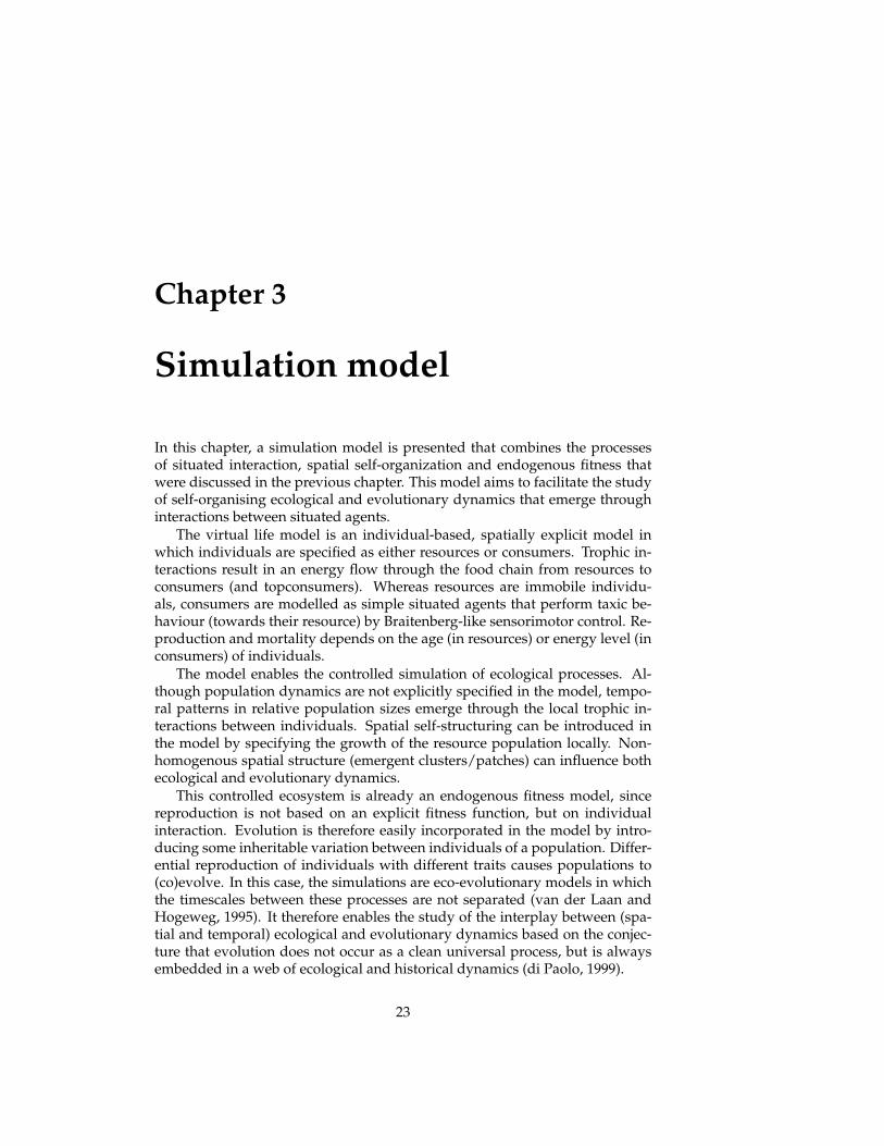
Figure 3.1: Screenshot of plants-herbivore simulation

This chapter overviews the most important aspects of the simulation model.The following section discusses the simulator in which the virtual life modelis implemented. Section 3.1 examines the main part of the model by describ-ing the specifications of individuals and populations, the trophic interactionsand evolutionary process, and providing an overview of the most importantsimulation parameters. The results of ecological experiments with emergentpopulation dynamics and spatial self-organization of resources are presentedin section 3.2. In section 3.3, conclusions are drawn from this chapter.

3.1 Virtual life model

Framsticks

The Virtual life simulation model is implemented in the a-life simulator whichallows customization for nearly all processes involved in the simulation byusing the scripting language FramScript (Komosinski and Ulatowski, 1999;Komosinski and Rotaru-Varga, 2000; Komosinski, 2003; Adamatzky and Ko-mosinski, 2005). The models presented here are simulations that are fully cus-tomized for ecological and evolutionary experiments. Among the features thatare adjusted to the Virtual life model are the physical simulation of the environ-ment, the sensors, control, and actuators of individuals, and most importantlythe experiment definition.

24

Algorithm 1 Basic structure of experiment definitionInitialization:- generate populations- fill population with individualsStep:- process sensors, control and update locations- if resource > reproductive age, reproduce (and mutate)- if consumer > reproductive energy, reproduce (and mutate)- subtract metabolistic energy of consumersInteraction (collision):- transfer energy from resource to consumer- if energy <= 0, kill individualInterval:- write population and genotype data to logfiles

Event-based

The experiment definition is an event-based program that tells the simulationwhat to do when certain events occur. This includes user events (e.g. loadingand initialization), interaction events (e.g. collisions between individuals), andpopulation events (e.g. spawning and removing individuals). This definitionis customized to implement an endogenous fitness model. The core of the Vir-tual life model is implemented as a set of experiment definitions that share thefollowing basic structure.

At initialization, populations of individuals are generated and certain amountsof individuals for each population are spawned in some locations in the envi-ronment. In evolutionary experiments, initial variation among individuals isinduced by stochastic mutations in a certain trait. The physical simulation, aswell as the processing of sensors, control and actuation (i.e. updating loca-tions) are left to the Framsticks simulator itself. However, most other aspectof individuals are updated every simulation step in this definition, such as ageand energy level. At a certain interval, data about observables are written tologfiles, such as population sizes and values of evolvable traits.

When collisions between individuals occur, the experiment definition de-termines whether these are ignored or handled. Collisions between con-specifics(individuals belonging to the same population) are ignored in the simulationsreported in this thesis (but can include e.g. sexual reproduction or dominanceinteractions). Inter-specific collisions are handled as trophic interactions interms of consumption and predation when certain conditions are met.

3.1.1 Environment

The environment is a continuous space in the form of a square (see fig. 3.1). Al-though the physical simulation in Framsticks simulates many physical forceson the mechanical bodies of creatures, these are largely ignored in these simu-lations. In the scope of this thesis, forces such as friction, inertia and gravity are

25

simulated but irrelevant for present purposes. Mechanical collisions betweenindividuals are ignored1.

Boundary conditions

The boundaries of the environment can be either fixed, wrapped around, or ab-sent. Different boundary condition can also be used for different populations2.Usually, resources are distributed only within the boundaries (fixed bound-aries). Consumers can, in principle, travel away from the environment (i.e.absent boundaries). However, they can only sustain themselves for a limitedtime and distance, since no resources are found outside the environment. Indi-viduals will die beyond a certain distance. Moreover, consumer individuals arecontrolled such that they turn in the direction of the highest sensory activationgradient, such that consumers are likely to stay relatively close to resources.

3.1.2 Populations

The environment is inhabited by individuals that belongs to a certain popula-tion. A population, or species, is a group of individuals that are equal in thefollowing respects. They consume (and are consumed by) the same species,they have the same (im)mobility, the same (metabolic) energy costs, reproduc-tive thresholds and evolvable traits. Populations are predefined by the modelin the sense that the interactions between individuals are defined for the popu-lations to which the individuals belong. These interactions determine the foodchain in which the populations are structured.

The implementation of the Virtual life model allows for many populationsto interact in intricate food webs, but the simulations in this thesis are restrictedto simple linear food chains of three species: a resource, consumer and topcon-sumer species.

Energy and trophic interactions

The flow of energy is a common theme in all ecosystems and it is a means ofunderstanding how all ecosystems having many properties in common irre-spective of their apparent differences. Therefore, it is often used as the keyfeature of individual-based ecological models and endogenous fitness evolu-tionary models.

Likewise, in the virtual life model, individuals are specified by an energylevel. The ecosystem is structured as a food chain, such that individuals of dif-ferent populations transfer their energy when they are consumed (see figure3.2). Energy is passed up the food chain every time an individual consumes

1The physical simulation may be important in future research that includes embodiment moreexplicitly, e.g. in studies in the coevolution of morphology and control.

2This can be convenient in simulations with consumers that require absent boundaries in com-bination with self-clustering resources that require fixed boundaries.

26

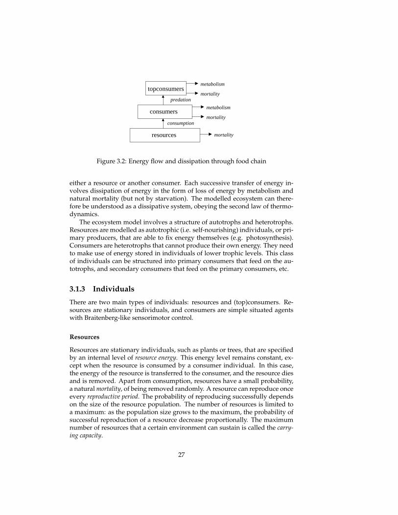
resources

consumers

topconsumers

consumption

predation

metabolism

mortality

mortality

metabolism

mortality

Figure 3.2: Energy flow and dissipation through food chain

either a resource or another consumer. Each successive transfer of energy in-volves dissipation of energy in the form of loss of energy by metabolism andnatural mortality (but not by starvation). The modelled ecosystem can there-fore be understood as a dissipative system, obeying the second law of thermo-dynamics.

The ecosystem model involves a structure of autotrophs and heterotrophs.Resources are modelled as autotrophic (i.e. self-nourishing) individuals, or pri-mary producers, that are able to fix energy themselves (e.g. photosynthesis).Consumers are heterotrophs that cannot produce their own energy. They needto make use of energy stored in individuals of lower trophic levels. This classof individuals can be structured into primary consumers that feed on the au-totrophs, and secondary consumers that feed on the primary consumers, etc.

3.1.3 Individuals

There are two main types of individuals: resources and (top)consumers. Re-sources are stationary individuals, and consumers are simple situated agentswith Braitenberg-like sensorimotor control.

Resources

Resources are stationary individuals, such as plants or trees, that are specifiedby an internal level of resource energy. This energy level remains constant, ex-cept when the resource is consumed by a consumer individual. In this case,the energy of the resource is transferred to the consumer, and the resource diesand is removed. Apart from consumption, resources have a small probability,a natural mortality, of being removed randomly. A resource can reproduce onceevery reproductive period. The probability of reproducing successfully dependson the size of the resource population. The number of resources is limited toa maximum: as the population size grows to the maximum, the probability ofsuccessful reproduction of a resource decrease proportionally. The maximumnumber of resources that a certain environment can sustain is called the carry-ing capacity.

27

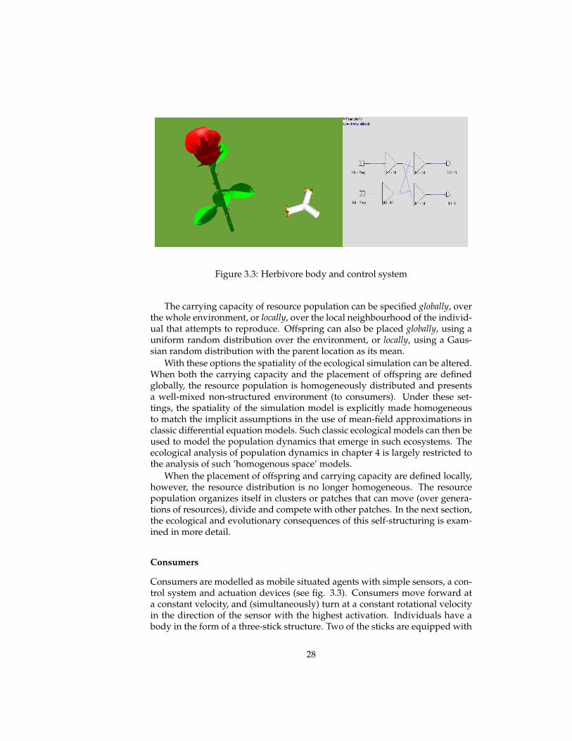
Figure 3.3: Herbivore body and control system

The carrying capacity of resource population can be specified globally, overthe whole environment, or locally, over the local neighbourhood of the individ-ual that attempts to reproduce. Offspring can also be placed globally, using auniform random distribution over the environment, or locally, using a Gaus-sian random distribution with the parent location as its mean.

With these options the spatiality of the ecological simulation can be altered.When both the carrying capacity and the placement of offspring are definedglobally, the resource population is homogeneously distributed and presentsa well-mixed non-structured environment (to consumers). Under these set-tings, the spatiality of the simulation model is explicitly made homogeneousto match the implicit assumptions in the use of mean-field approximations inclassic differential equation models. Such classic ecological models can then beused to model the population dynamics that emerge in such ecosystems. Theecological analysis of population dynamics in chapter 4 is largely restricted tothe analysis of such ’homogenous space’ models.

When the placement of offspring and carrying capacity are defined locally,however, the resource distribution is no longer homogeneous. The resourcepopulation organizes itself in clusters or patches that can move (over genera-tions of resources), divide and compete with other patches. In the next section,the ecological and evolutionary consequences of this self-structuring is exam-ined in more detail.

Consumers

Consumers are modelled as mobile situated agents with simple sensors, a con-trol system and actuation devices (see fig. 3.3). Consumers move forward ata constant velocity, and (simultaneously) turn at a constant rotational velocityin the direction of the sensor with the highest activation. Individuals have abody in the form of a three-stick structure. Two of the sticks are equipped with

28

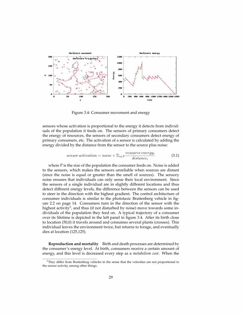
Figure 3.4: Consumer movement and energy

sensors whose activation is proportional to the energy it detects from individ-uals of the population it feeds on. The sensors of primary consumers detectthe energy of resources, the sensors of secondary consumers detect energy ofprimary consumers, etc. The activation of a sensor is calculated by adding theenergy divided by the distance from the sensor to the source plus noise:

sensor activation = noise + Σi∈Presource energyi

distancei(3.1)

where P is the size of the population the consumer feeds on. Noise is addedto the sensors, which makes the sensors unreliable when sources are distant(since the noise is equal or greater than the smell of sources). The sensorynoise ensures that individuals can only sense their local environment. Sincethe sensors of a single individual are in slightly different locations and thusdetect different energy levels, the difference between the sensors can be usedto steer in the direction with the highest gradient. The control architecture ofconsumer individuals is similar to the phototaxic Braitenberg vehicle in fig-ure 2.2 on page 14. Consumers turn in the direction of the sensor with thehighest activity3, and thus (if not disturbed by noise) move towards some in-dividuals of the population they feed on. A typical trajectory of a consumerover its lifetime is depicted in the left panel in figure 3.4. After its birth closeto location (50,0) it travels around and consumes several plants (crosses). Thisindividual leaves the environment twice, but returns to forage, and eventuallydies at location (125,125).

Reproduction and mortality Birth and death processes are determined bythe consumer’s energy level. At birth, consumers receive a certain amount ofenergy, and this level is decreased every step as a metabolism cost. When the

3They differ from Braitenberg vehicles in the sense that the velocities are not proportional tothe sensor activity, among other things.

29

energy is below zero, the individual dies and is removed from the environ-ment. Energy levels can be increased by consumption during which energy istransferred from the resource to consumer. When the energy level exceeds thereproduction energy, the individual reproduces. Offspring receives half of theenergy of its parent.

The right panel in figure 3.4 shows the energy level over the lifetime ofa consumer. It decreases linearly every step and increasing instantly on con-sumption. When the energy level rises above the reproductive threshold (of1000), it reproduces and half of its energy in inherited by (or invested in) theoffspring. After a period of sustaining a constant energy level, the consumerdies of starvation.

Placement of offspring The spatial placement of offspring can be done inseveral ways. They can be placed (1) in a random location in the environment,(2) close to its parent, and (3) close to a random parent. The first can be usedto approach the homogeneity that is assumed by classic differential equationmodels, and thus can be understood better in the terms of such models. Thesecond introduces spatial heterogeneity that potentially influences ecologicaland evolutionary dynamics, and the third placement option is used to showthis influence by distorting the correlation between spatial and genetic related-ness.

3.1.4 Evolution

Evolution is easily incorporated in the model by having some inheritable vari-ation among individuals in the populations. Within the scope of this thesis, theevolution dynamics are extremely simple. Individuals are specified by only asingle trait, restricting the evolution of the population to a single dimension.Moreover, simple one-to-one genotype-to-phenotype mapping are used, andlearning or development processes are excluded.

When an individual reproduces its offspring inherits its genotype (=phe-notype), while mutations occur with a certain mutation probability. Mutationson real-valued genotypes are usually modelled as Gaussian diffusion, and bymutating natural-valued genotypes is done by altering the parent genotype byadding or substracting one. In coevolutionary experiments, the mutation prob-abilities are equal for the populations involved. Phenotypic traits are chosensuch that there is a clear relationship to parameters in the theoretical modeland the evolvable trait.

Evolution is not included from the ecological experiments presented in thisand the next chapter, in which all individuals are identical. Evolutionary dy-namics that emerge from the simulation model are explored in more detail inchapter 5.

30

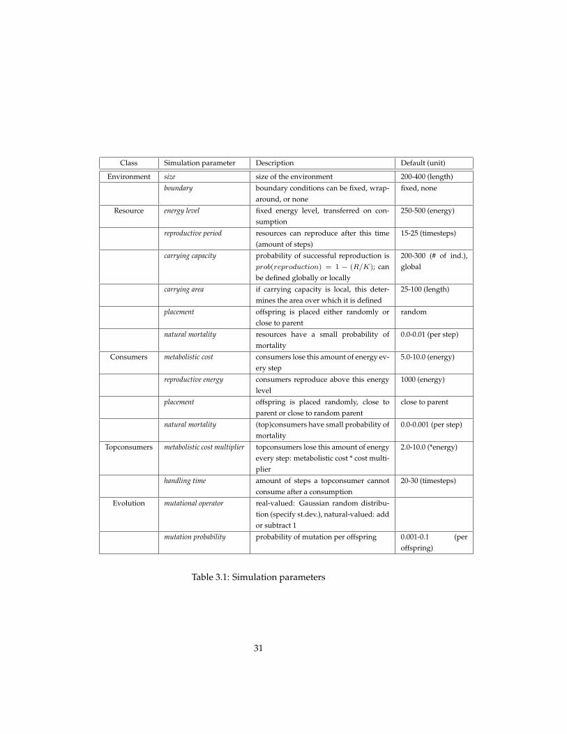
Class Simulation parameter Description Default (unit)

Environment size size of the environment 200-400 (length)

boundary boundary conditions can be fixed, wrap-around, or none

fixed, none

Resource energy level fixed energy level, transferred on con-sumption

250-500 (energy)

reproductive period resources can reproduce after this time(amount of steps)

15-25 (timesteps)

carrying capacity probability of successful reproduction isprob(reproduction) = 1 − (R/K); canbe defined globally or locally

200-300 (# of ind.),global

carrying area if carrying capacity is local, this deter-mines the area over which it is defined

25-100 (length)

placement offspring is placed either randomly orclose to parent

random

natural mortality resources have a small probability ofmortality

0.0-0.01 (per step)

Consumers metabolistic cost consumers lose this amount of energy ev-ery step

5.0-10.0 (energy)

reproductive energy consumers reproduce above this energylevel

1000 (energy)

placement offspring is placed randomly, close toparent or close to random parent

close to parent

natural mortality (top)consumers have small probability ofmortality

0.0-0.001 (per step)

Topconsumers metabolistic cost multiplier topconsumers lose this amount of energyevery step: metabolistic cost * cost multi-plier

2.0-10.0 (*energy)

handling time amount of steps a topconsumer cannotconsume after a consumption

20-30 (timesteps)

Evolution mutational operator real-valued: Gaussian random distribu-tion (specify st.dev.), natural-valued: addor subtract 1

mutation probability probability of mutation per offspring 0.001-0.1 (peroffspring)

Table 3.1: Simulation parameters

31

3.1.5 Simulation parameters

In the above description of the model, various simulation parameters havebeen discussed that influences spatial, energetic, reproductive and mutationalprocesses in the simulated ecosystem. An overview of the most important sim-ulation parameters is given in table 3.1.

These parameters enable us to influence simulated (evolving) ecosystemsin many ways. The results of various experiments studying the influence ofparameter settings are reported in the next section. In the next chapter, thesesimulation parameters are related to parameters in theoretical ecological mod-els. Correspondences between these two enable us to manipulate the ecologicaland evolutionary dynamics.

3.2 Emergent patterns

The simulated ecosystem, consisting of many interacting individuals, can beunderstood as a self-organizing dissipative system. The energy flow throughthe food chain results in temporal patterns in population sizes, or in spatial pat-tern formation of resources. In this section, several emergent patterns resultingfrom ecological simulations are reported.

Two sets of simulation experiments are conducted. First, simulations withthe virtual life model are conducted with a resource-consumer and a resource-consumer-topconsumer system. These experiments focus on the populationdynamics that emerge through the trophic interactions in a homogeneous en-vironment. Second, the influence of spatial self-structuring on ecological andevolutionary scales is studied by a simulation of only a resource population.

3.2.1 Population dynamics

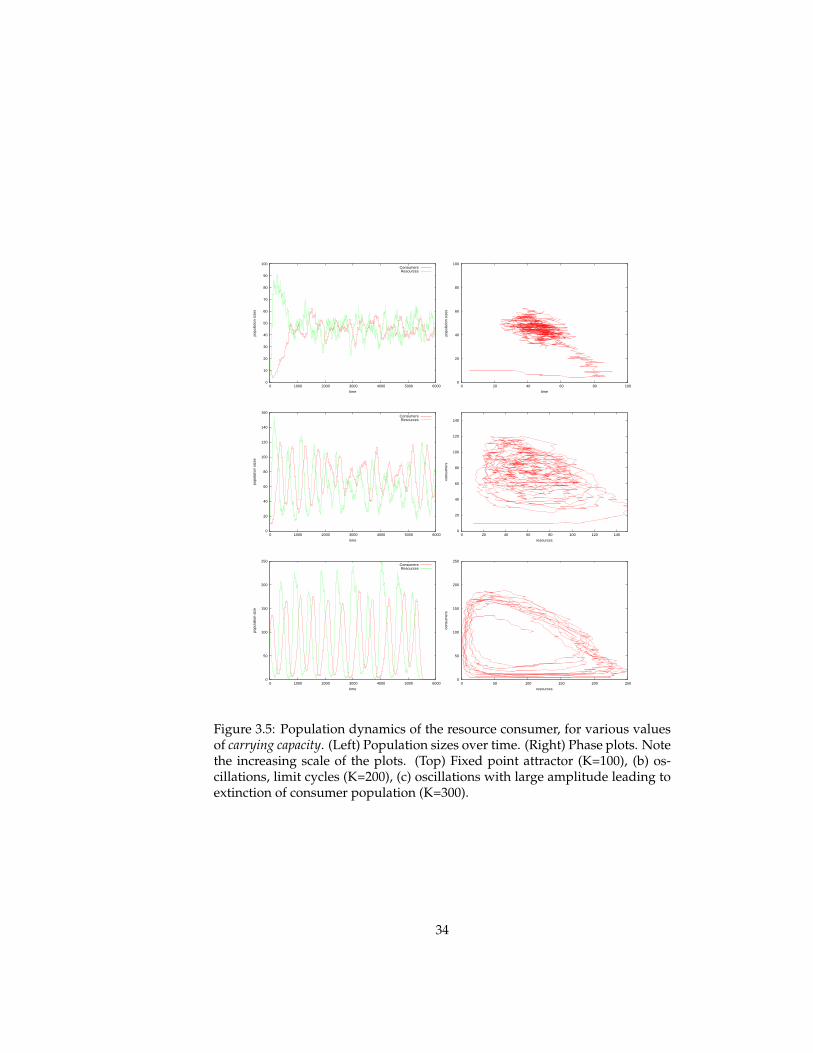
To study population dynamics in the virtual life model, a simple ecosystemwith a resource and consumer population is simulated. Trophic interactions be-tween resources and consumers result in changes in population sizes over time.The emergent population dynamics show nonlinear behaviors such as fixedpoints attractors, limit cycle oscillations and strange attractors. The resultsof simulation of a resource-consumer and a resource-consumer-topconsumerecosystem are presented below. In these experiments, the spatial distributionof resources was defined globally to obtain spatial homogeneity.

Resource-Consumer ecosystem The ecosystem model is initialised witha resource and a consumer population. The simulation parameters are shownin figure 3.2.

Figure 3.5 shows the resulting population dynamics, transients and phaseplots, for three different values of the carrying capacity. The panels in the toprow show population dynamics that approach a stable fixed point equilibrium,with random fluctuation. The population dynamics in the second row exhibit

32

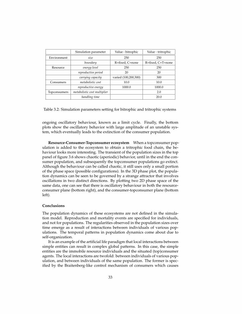
Simulation parameter Value - bitrophic Value - tritrophic

Environment size 250 250

boundary R=fixed, C=none R=fixed, C=T=none

Resource energy level 250 250

reproductive period 20 20

carrying capacity varied (100,200,300) 300

Consumers metabolistic cost 10.0 10.0

reproductive energy 1000.0 1000.0

Topconsumers metabolistic cost multiplier 2.0

handling time 20.0

Table 3.2: Simulation parameters setting for bitrophic and tritrophic systems

ongoing oscillatory behaviour, known as a limit cycle. Finally, the bottomplots show the oscillatory behavior with large amplitude of an unstable sys-tem, which eventually leads to the extinction of the consumer population.

Resource-Consumer-Topconsumer ecosystem When a topconsumer pop-ulation is added to the ecosystem to obtain a tritrophic food chain, the be-haviour looks more interesting. The transient of the population sizes in the toppanel of figure 3.6 shows chaotic (aperiodic) behavior, until in the end the con-sumer population, and subsequently the topconsumer populations go extinct.Although the behaviour can be called chaotic, it still uses only a small portionof the phase space (possible configurations). In the 3D phase plot, the popula-tion dynamics can be seen to be governed by a strange attractor that involvesoscillations in two distinct directions. By plotting two 2D phase space of thesame data, one can see that there is oscillatory behaviour in both the resource-consumer plane (bottom right), and the consumer-topconsumer plane (bottomleft).

Conclusions

The population dynamics of these ecosystems are not defined in the simula-tion model. Reproduction and mortality events are specified for individuals,and not for populations. The regularities observed in the population sizes overtime emerge as a result of interactions between individuals of various pop-ulations. The temporal patterns in population dynamics come about due toself-organization.

It is an example of the artificial life paradigm that local interactions betweensimple entities can result in complex global patterns. In this case, the simpleentities are the immobile resource individuals and the situated (top)consumeragents. The local interactions are twofold: between individuals of various pop-ulation, and between individuals of the same population. The former is spec-ified by the Braitenberg-like control mechanism of consumers which causes

33

0

10

20

30

40

50

60

70

80

90

100

0 1000 2000 3000 4000 5000 6000

popu

latio

n si

zes

time

ConsumersResources

0

20

40

60

80

100

0 20 40 60 80 100

popu

latio

n si

zes

time

0

20

40

60

80

100

120

140

160

0 1000 2000 3000 4000 5000 6000

popu

latio

n si

zes

time

ConsumersResources

0

20

40

60

80

100

120

140

0 20 40 60 80 100 120 140

cons

umer

s

resources

0

50

100

150

200

250

0 1000 2000 3000 4000 5000 6000

popu

latio

n si

ze

time

ConsumersResources

0

50

100

150

200

250

0 50 100 150 200 250

cons

umer

s

resources

Figure 3.5: Population dynamics of the resource consumer, for various valuesof carrying capacity. (Left) Population sizes over time. (Right) Phase plots. Notethe increasing scale of the plots. (Top) Fixed point attractor (K=100), (b) os-cillations, limit cycles (K=200), (c) oscillations with large amplitude leading toextinction of consumer population (K=300).

34

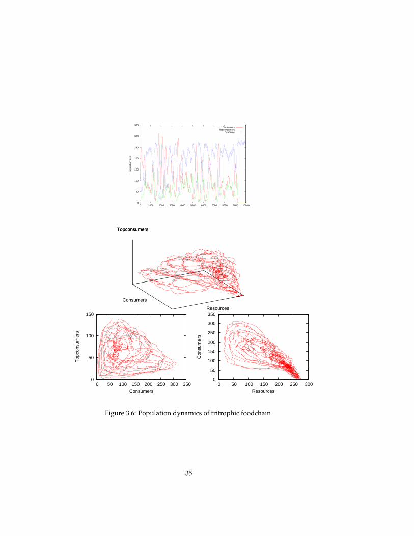
0

50

100

150

200

250

300

350

0 1000 2000 3000 4000 5000 6000 7000 8000 9000 10000

popu

latio

n si

zeConsumers

TopconsumersResource

Topconsumers

Resources

Consumers

Topconsumers

0

50

100

150

200

250

300

350

0 50 100 150 200 250 300

Con

sum

ers

Resources

0

50

100

150

0 50 100 150 200 250 300 350

Top

cons

umer

s

Consumers

Figure 3.6: Population dynamics of tritrophic foodchain

35

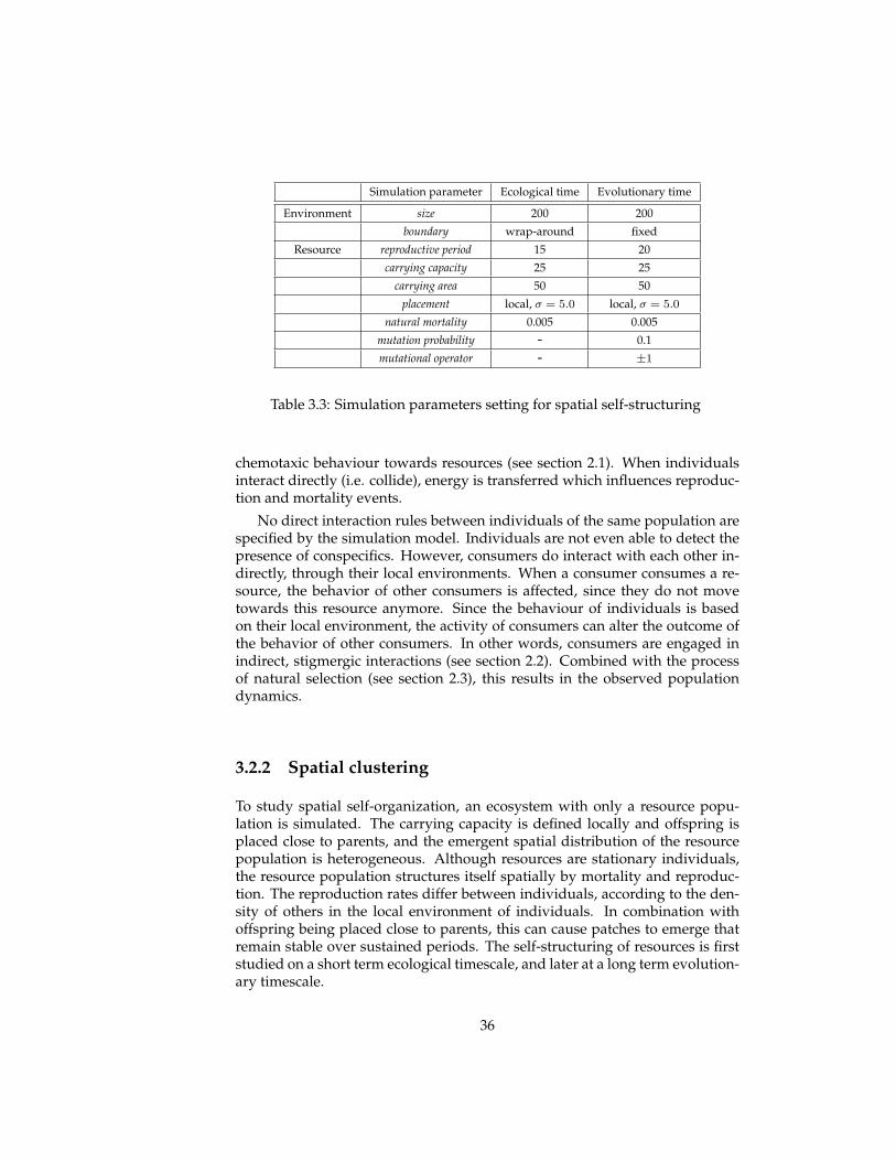
Simulation parameter Ecological time Evolutionary time

Environment size 200 200

boundary wrap-around fixed

Resource reproductive period 15 20

carrying capacity 25 25

carrying area 50 50

placement local, σ = 5.0 local, σ = 5.0

natural mortality 0.005 0.005

mutation probability - 0.1

mutational operator - ±1

Table 3.3: Simulation parameters setting for spatial self-structuring

chemotaxic behaviour towards resources (see section 2.1). When individualsinteract directly (i.e. collide), energy is transferred which influences reproduc-tion and mortality events.

No direct interaction rules between individuals of the same population arespecified by the simulation model. Individuals are not even able to detect thepresence of conspecifics. However, consumers do interact with each other in-directly, through their local environments. When a consumer consumes a re-source, the behavior of other consumers is affected, since they do not movetowards this resource anymore. Since the behaviour of individuals is basedon their local environment, the activity of consumers can alter the outcome ofthe behavior of other consumers. In other words, consumers are engaged inindirect, stigmergic interactions (see section 2.2). Combined with the processof natural selection (see section 2.3), this results in the observed populationdynamics.

3.2.2 Spatial clustering

To study spatial self-organization, an ecosystem with only a resource popu-lation is simulated. The carrying capacity is defined locally and offspring isplaced close to parents, and the emergent spatial distribution of the resourcepopulation is heterogeneous. Although resources are stationary individuals,the resource population structures itself spatially by mortality and reproduc-tion. The reproduction rates differ between individuals, according to the den-sity of others in the local environment of individuals. In combination withoffspring being placed close to parents, this can cause patches to emerge thatremain stable over sustained periods. The self-structuring of resources is firststudied on a short term ecological timescale, and later at a long term evolution-ary timescale.

36

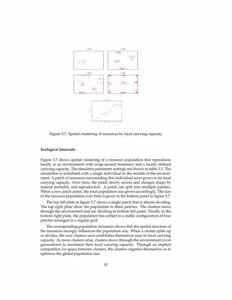
t = 1000 t = 3000

t = 4000 t = 5000

0

100

200

300

400

0 1000 2000 3000 4000 5000 6000 7000

Pop

ulat

ion

size

time

Resource population size

Figure 3.7: Spatial clustering of resources by local carrying capacity

Ecological timescale

Figure 3.7 shows spatial clustering of a resource population that reproduceslocally in an environment with wrap-around boundary and a locally definedcarrying capacity. The simulator parameter settings are shown in table 3.3. Thesimulation is initialised with a single individual in the middle of the environ-ment. A patch of resources surrounding this individual soon grows to its localcarrying capacity. Over time, the patch slowly moves and changes shape bynatural mortality and reproduction. A patch can split into multiple patches.When a new patch arises, the total population size grows accordingly. The sizeof the resource population over time is given in the bottom panel in figure 3.7.

The top left plate in figure 3.7 shows a single patch that is almost dividing.The top right plate show the population in three patches. The clusters movethrough the environment and are dividing in bottom left panel. Finally, in thebottom right plate, the population has settled in a stable configuration of fourpatches arranged in a regular grid.

The corresponding population dynamics shows that the spatial structure ofthe resources strongly influences the population size. When a cluster splits upor divides, the new clusters soon establishes themselves near its local carryingcapacity. As more clusters arise, clusters move through the environment (overgenerations) to maximize their local carrying capacity. Through an implicitcompetition for space between clusters, the clusters organise themselves as tooptimize the global population size.

37

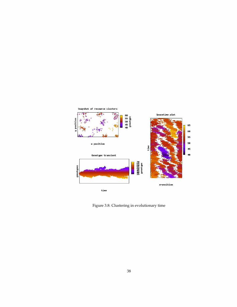
Figure 3.8: Clustering in evolutionary time

38

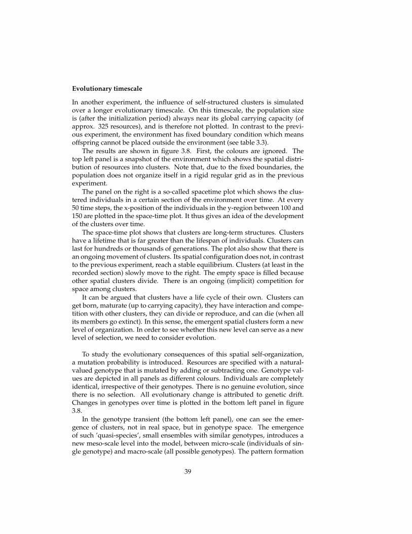
Evolutionary timescale

In another experiment, the influence of self-structured clusters is simulatedover a longer evolutionary timescale. On this timescale, the population sizeis (after the initialization period) always near its global carrying capacity (ofapprox. 325 resources), and is therefore not plotted. In contrast to the previ-ous experiment, the environment has fixed boundary condition which meansoffspring cannot be placed outside the environment (see table 3.3).

The results are shown in figure 3.8. First, the colours are ignored. Thetop left panel is a snapshot of the environment which shows the spatial distri-bution of resources into clusters. Note that, due to the fixed boundaries, thepopulation does not organize itself in a rigid regular grid as in the previousexperiment.

The panel on the right is a so-called spacetime plot which shows the clus-tered individuals in a certain section of the environment over time. At every50 time steps, the x-position of the individuals in the y-region between 100 and150 are plotted in the space-time plot. It thus gives an idea of the developmentof the clusters over time.

The space-time plot shows that clusters are long-term structures. Clustershave a lifetime that is far greater than the lifespan of individuals. Clusters canlast for hundreds or thousands of generations. The plot also show that there isan ongoing movement of clusters. Its spatial configuration does not, in contrastto the previous experiment, reach a stable equilibrium. Clusters (at least in therecorded section) slowly move to the right. The empty space is filled becauseother spatial clusters divide. There is an ongoing (implicit) competition forspace among clusters.

It can be argued that clusters have a life cycle of their own. Clusters canget born, maturate (up to carrying capacity), they have interaction and compe-tition with other clusters, they can divide or reproduce, and can die (when allits members go extinct). In this sense, the emergent spatial clusters form a newlevel of organization. In order to see whether this new level can serve as a newlevel of selection, we need to consider evolution.

To study the evolutionary consequences of this spatial self-organization,a mutation probability is introduced. Resources are specified with a natural-valued genotype that is mutated by adding or subtracting one. Genotype val-ues are depicted in all panels as different colours. Individuals are completelyidentical, irrespective of their genotypes. There is no genuine evolution, sincethere is no selection. All evolutionary change is attributed to genetic drift.Changes in genotypes over time is plotted in the bottom left panel in figure3.8.

In the genotype transient (the bottom left panel), one can see the emer-gence of clusters, not in real space, but in genotype space. The emergenceof such ’quasi-species’, small ensembles with similar genotypes, introduces anew meso-scale level into the model, between micro-scale (individuals of sin-gle genotype) and macro-scale (all possible genotypes). The pattern formation

39

in genotype space can lead to an interlocking of ecological and evolutionarytimescales (van der Laan and Hogeweg, 1995).

The genotypic clusters can be seen in the space-time plot as well. By look-ing at the colours of the various clusters (in real space), the genetic similaritywithin the spatial clusters is evidently higher than between clusters. An exam-ple of a correlated spatial/genotypic cluster can be seen in the middle of thespace-time plot (blue/purple/black cluster), which corresponds to the clusterin the middle of the genotype transient. The snapshot also shows a strong cor-relation between spatial relatedness and genetic relatedness, since the colourswithin a cluster are more similar then the colours between clusters.

This experiment does not include evolution in the sense of a mutation-selection mechanism, since there is no selection (acting upon geno- or phe-notypes). It does show, however, that the formation of a new level or organi-zation (i.e. the spatial/genotypic clusters) introduces a new level of historicaldependence to the dynamics of the system over evolutionary timescale. Thishistorical dependence causes a diversity of genotypes in spatial clusters, whichintroduces a new level on which selection can act.

Conclusions

The spatial structuring is not specified by the simulation model. Therefore, thesimulation model only specifies the conditions that allow spatial self-organizationto occur. The clusters of resource that appear over time are not predefined, butemerge through interactions between resources that stem from the local defini-tions of carrying capacity and placement of offspring.

3.3 Conclusions

This chapter described the key features of the virtual life simulation model:the simulated environment, the resource and consumer individuals that in-habit this environment and how they are structured in a trophic food chain.Nonlinear population dynamics emerge from the (trophic and behavioural) in-teractions between stationary resources and situated (top)consumers, due toa combination of stigmergic and energetic processes. Spatial self-structuringof the resource population occurs under local conditions for placement of off-spring and carrying capacity. The emergent spatial clusters or patches intro-duce a new level of organisation (between individual and population) that caninfluence ecological dynamics and evolutionary dynamics.

The population dynamics are analysed in terms of differential equationmodels by mean-field approximation in the next chapter. This enables us togain theoretical understanding of the dynamics that emerge from the simu-lation models. The correspondence and relations between the simulation pa-rameters and the parameters in the theoretical model enable us to predict andmanipulate the population dynamics in ecological and evolutionary contexts.

40

Chapter 4

Ecological analysis

The simulation model described in the previous chapter showed the emer-gence of complex bi- and tritrophic population dynamics. In order to under-stand, predict and control these ecological dynamics, a corresponding theoret-ical framework is developed in this chapter. The density dependencies of thevarious ecological processes (e.g. population growth, consumption, mortality)that arise from the model are experimentally determined and put together ina classical ecological model that consist of a set of ordinary differential equa-tions. The models obtained in this fashion allow us to gain insight into theemergent dynamics in two ways: (1) it enables the control and prediction of theecological dynamical consequences by of changes in simulation parameters orevolutionary changes (discussed in next chapter), (2) it provides a theoreticalbasis to study the consequences of lifting some of the assumptions implicit inthe classical model.

The goal of the simulation model, and in fact of all individual-based modelsin theoretical biology and ecology, is to allow modelers to investigate questionsthat have been difficult or impossible to address using a classical state-variableapproach (Hutson et al., 1988). The state variables most often used in ecol-ogy are population numbers or densities, and the ecosystem is described interms of changes thereof in space and/or time. In contrast, individual-basedmodels use individuals as their basic unit. The homogeneity assumed in clas-sical models, caused by ’lumping’ individuals in population averages, makesthem inappropriate to study the self-organization of spatiotemporal patternsthat arise from local interaction between individuals (Hogeweg and Hesper,1990).

The self-organised spatial clustering and temporal patterns in populationdynamics observed in the simulation model in the previous chapter were notpart of the model specifications itself. Rather, they emerged from the behaviouraland trophic interactions between individuals. This, however, does not neces-sarily imply that classical models are inappropriate to analyse these dynamics,as the regularities observed in the population dynamics (in figs. 3.5 and 3.6)already suggested. In these cases, the simulation model was constructed in co-

41

herence with some classical assumptions. The populations are monomorphicsince all individuals in a population are equal. And the spatial distributionis approximately homogeneous, because all offspring is placed at a randomlocation in the environment.1

The most interesting phenomena are of course observed in situations wherethese assumptions are lifted, and the spatial and individual-based nature of thesimulation model gives rise to qualitatively different outcomes. This will beshown in the evolutionary and spatially heterogeneous experiments in chapter5. The classical model that is developed in this chapter serves as the theoreticalframework in which the consequences of these changes can be studied.

In section 4.1, the various ecological processes in and between the resourceand consumer population are experimentally determined and theoretically mod-elled. These processes are combined to form theoretical models for bitrophicand tritrophic ecosystems, for which a brief qualitative analysis is provided insection 4.2. Section 4.3 discussed the way in which these models allows us tomanipulate and control the emergent population dynamics, and conclusionsare drawn in section 4.4.

4.1 Resource and consumer dynamics

The increase and decrease of population sizes of resources and consumers de-pends on various factors. In this section, the various density dependent pro-cesses are modelled by examining the specification of the simulation modelitself or the emergent processes it gives rise to.

4.1.1 Resource dynamics

To determine the change of the population size of the resource population overtime, we first consider the simple situation of an ecosystem consisting of a re-source population without consumers (C = 0). Resources can reproduce after acertain reproductive period, causing a fast growth at low values, and slow pop-ulation growth at high values. The density dependence of the reproductionrate is explicitly defined by the simulation model. The probability of success-ful reproduction is determined by the difference between current populationsize and a user-defined carrying capacity. The resulting population dynam-ics shows a logistic growth. Such population growth can be described by theVerhulst or logistic model:

dR

dt= rR(1− R

K) (4.1)

where r = 1/reproductive period and K = carrying capacity. A negativeterm dR can be included if natural mortality of resource is nonzero.

1The simulation does not comply with the assumption of infinite populations, however. Thepopulations in the simulation model are discrete and small.

42

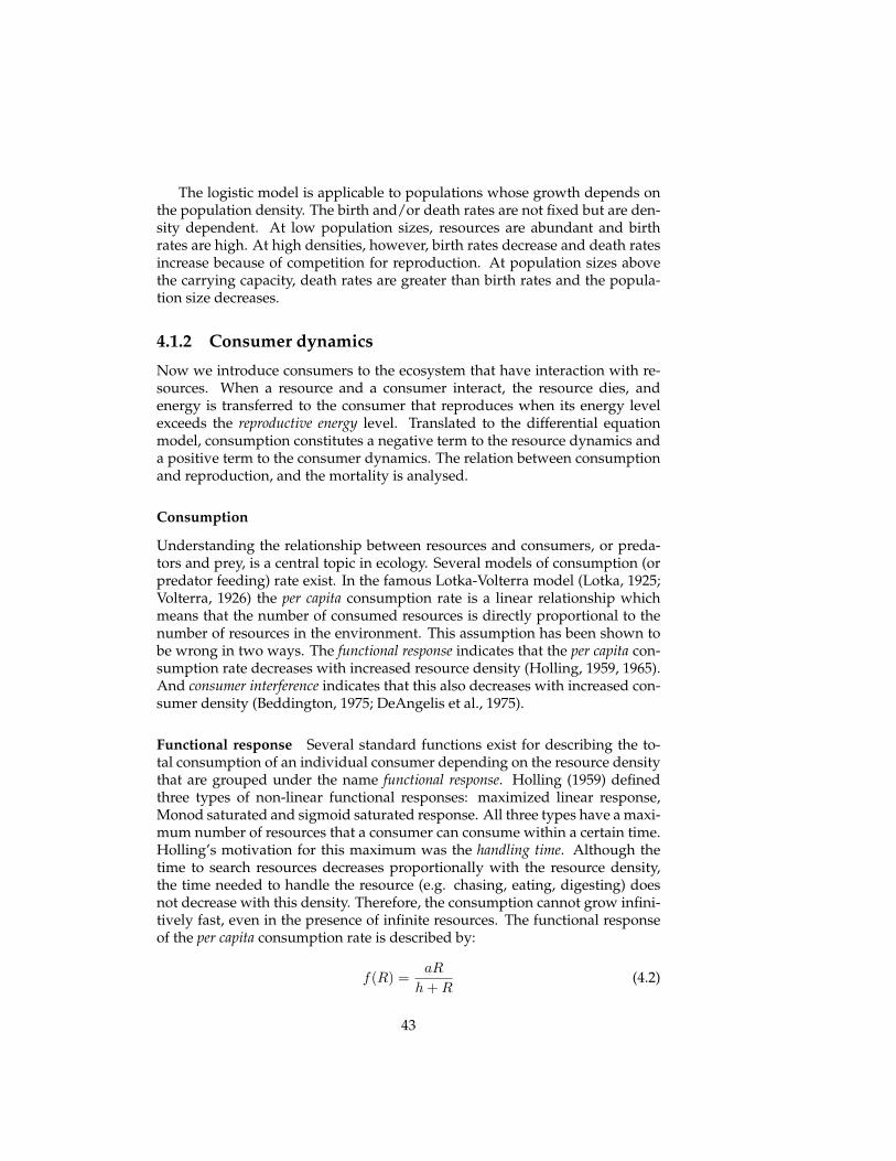
The logistic model is applicable to populations whose growth depends onthe population density. The birth and/or death rates are not fixed but are den-sity dependent. At low population sizes, resources are abundant and birthrates are high. At high densities, however, birth rates decrease and death ratesincrease because of competition for reproduction. At population sizes abovethe carrying capacity, death rates are greater than birth rates and the popula-tion size decreases.

4.1.2 Consumer dynamics

Now we introduce consumers to the ecosystem that have interaction with re-sources. When a resource and a consumer interact, the resource dies, andenergy is transferred to the consumer that reproduces when its energy levelexceeds the reproductive energy level. Translated to the differential equationmodel, consumption constitutes a negative term to the resource dynamics anda positive term to the consumer dynamics. The relation between consumptionand reproduction, and the mortality is analysed.

Consumption

Understanding the relationship between resources and consumers, or preda-tors and prey, is a central topic in ecology. Several models of consumption (orpredator feeding) rate exist. In the famous Lotka-Volterra model (Lotka, 1925;Volterra, 1926) the per capita consumption rate is a linear relationship whichmeans that the number of consumed resources is directly proportional to thenumber of resources in the environment. This assumption has been shown tobe wrong in two ways. The functional response indicates that the per capita con-sumption rate decreases with increased resource density (Holling, 1959, 1965).And consumer interference indicates that this also decreases with increased con-sumer density (Beddington, 1975; DeAngelis et al., 1975).

Functional response Several standard functions exist for describing the to-tal consumption of an individual consumer depending on the resource densitythat are grouped under the name functional response. Holling (1959) definedthree types of non-linear functional responses: maximized linear response,Monod saturated and sigmoid saturated response. All three types have a maxi-mum number of resources that a consumer can consume within a certain time.Holling’s motivation for this maximum was the handling time. Although thetime to search resources decreases proportionally with the resource density,the time needed to handle the resource (e.g. chasing, eating, digesting) doesnot decrease with this density. Therefore, the consumption cannot grow infini-tively fast, even in the presence of infinite resources. The functional responseof the per capita consumption rate is described by:

f(R) =aR

h + R(4.2)

43

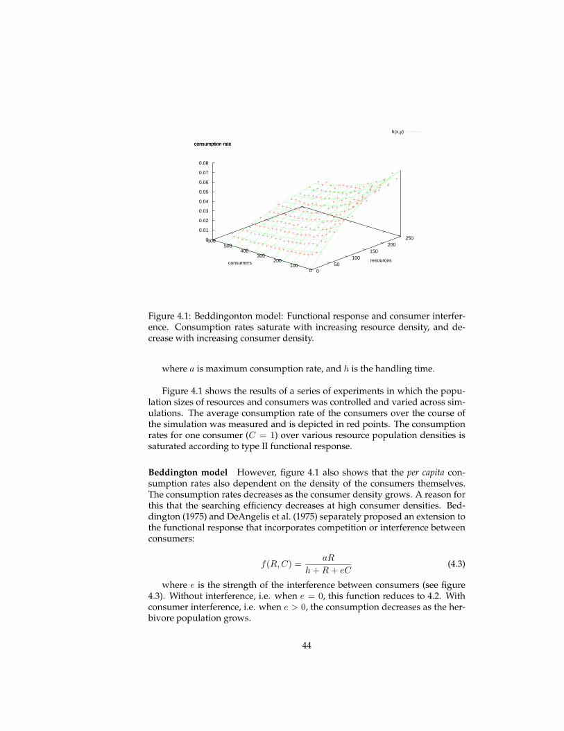
0 50

100 150

200 250

0 100

200 300

400 500

600 0

0.01

0.02

0.03

0.04

0.05

0.06

0.07

0.08

consumption rate

h(x,y)

resourcesconsumers

consumption rate

Figure 4.1: Beddingonton model: Functional response and consumer interfer-ence. Consumption rates saturate with increasing resource density, and de-crease with increasing consumer density.

where a is maximum consumption rate, and h is the handling time.

Figure 4.1 shows the results of a series of experiments in which the popu-lation sizes of resources and consumers was controlled and varied across sim-ulations. The average consumption rate of the consumers over the course ofthe simulation was measured and is depicted in red points. The consumptionrates for one consumer (C = 1) over various resource population densities issaturated according to type II functional response.

Beddington model However, figure 4.1 also shows that the per capita con-sumption rates also dependent on the density of the consumers themselves.The consumption rates decreases as the consumer density grows. A reason forthis that the searching efficiency decreases at high consumer densities. Bed-dington (1975) and DeAngelis et al. (1975) separately proposed an extension tothe functional response that incorporates competition or interference betweenconsumers:

f(R,C) =aR

h + R + eC(4.3)

where e is the strength of the interference between consumers (see figure4.3). Without interference, i.e. when e = 0, this function reduces to 4.2. Withconsumer interference, i.e. when e > 0, the consumption decreases as the her-bivore population grows.

44

0

0.01

0.02

0.03

0.04

0.05

0.06

0.07

0 0.02 0.04 0.06 0.08 0.1 0.12 0.14

repr

oduc

tion

rate

consumption rate

0

0.0002

0.0004

0.0006

0.0008

0.001

0.0012

0.0014

0 50 100 150 200 250

cons

umer

mor

talit

y ra

te

resources

Figure 4.2: (Left) Linear conversion of consumed resources to consumer off-spring. (Right) Mortality rate .

Reproduction

Most ecological resource-consumer models abide the conversion rule whichstates that the consumer reproduction rate is a function of its consumption rate(Ginzburg, 1998). In the simulation model, reproduction is based on individualenergy levels, which can only be increased by consumption. It can thus beexpected that the reproduction rate and consumption rate will show a strongcorrelation and this is evident from figure 4.2 which plot the linear relationshipbetween them. The conversion efficiency coefficient c is the slope of this line.

Mortality

Eventually, consumers die of starvation. The right panel in figure 4.2 showsthat the per capita mortality rate depends on the resource density, according tothe function:

f(R) = d− dR

i + R(4.4)

where d is the death or mortality rate, which is maximal when R = 0 (noresources), and half its maximum when R = i.

The conducted experiments show no dependence on consumer density,however. In the ecological models that are used in the following, the per capitamortality is simplified to be constant.

4.2 Ecological models

In the previous paragraphs, the various functional dependencies of the re-source and consumer populations were examined. These relations are the com-ponents of the ecological model that is constructed in this section. By putting

45

the functional relations together in a set of differential equations, a theoreticalmodel is obtained that captures the dynamics of the population dynamics thatare observed in the simulations described in chapter 3. A mathematical andgraphical analysis of such a simplified ’mini-model’ allows us to gain insightinto qualitative and quantitative aspects of the emergent population dynam-ics. Moreover, the relation between the simulation model to some well-studiedtheoretical models enables us to make use of the existing ecological literaturethat deals with these models.

In this section, theoretical models are constructed from the components laiddown in the previous section that model the population dynamics of the bi-trophic (two-species) and tritrophic (three-species) food chains, as observed insection 3.2. In the construction and analysis of these models, a graphical ap-proach is adopted (in which we follow de Boer (2006)).

4.2.1 Bitrophic model

To establish an ecological model describing the population dynamics of a bi-trophic ecosystem, as shown in figure 3.5, the functions describing logistic re-source population growth (eq. 4.1), Beddington consumption (eq. 4.3), linearconsumer conversion and constant per capita mortality are combined2:

dR

dt= rR(1− R

K)− aRC

h + R + eCdC

dt=

caRC

h + R + eC− dC (4.5)

This ecological model enables us to study the behaviour of this system bygraphical phase space analysis. This does not give us analytical or numericalsolutions, but it does give us insight into the behaviour of the system over time.To do a graphical analysis, the nullclines of the system and its steady states arecalculated, and sketched in a phase space diagram with a vector field. Null-clines are graphs of the set of points in the phase space for which the change ofa population is zero, and steady states are located at intersections of nullclines.

The nullcline of the consumer population in the model 4.5 is obtained bysolving the system when setting dC/dt = 0:

dC

dt= 0 → C = 0 ∨ C =

ca− d

deR− h

e=

R0 − 1e

R− h

e(4.6)

where R0 = ca/d represent the per capita consumption-dependent birth rateca of individuals over their expected life span of 1/d time units. This gives the

2In the construction of the model in eq. 4.5 some simplifications are made: natural mortality ofresources (apart from consumption-induced mortality) is not included, and the per capita mortalityof consumers is simplified to a constant mortality.

46

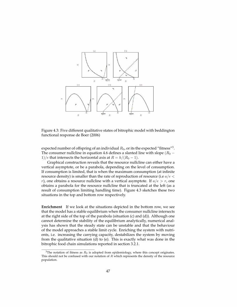
Figure 4.3: Five different qualitative states of bitrophic model with beddingtonfunctional response de Boer (2006)

expected number of offspring of an individual R0, or its the expected “fitness”3.The consumer nullcline in equation 4.6 defines a slanted line with slope (R0 −1)/e that intersects the horizontal axis at R = h/(R0 − 1).

Graphical construction reveals that the resource nullcline can either have avertical asymptote, or be a parabola, depending on the level of consumption.If consumption is limited, that is when the maximum consumption (at infiniteresource density) is smaller than the rate of reproduction of resource (i.e a/e <r), one obtains a resource nullcline with a vertical asymptote. If a/e > r, oneobtains a parabola for the resource nullcline that is truncated at the left (as aresult of consumption limiting handling time). Figure 4.3 sketches these twosituations in the top and bottom row respectively.

Enrichment If we look at the situations depicted in the bottom row, we seethat the model has a stable equilibrium when the consumer nullcline intersectsat the right side of the top of the parabola (situation (c) and (d)). Although onecannot determine the stability of the equilibrium analytically, numerical anal-ysis has shown that the steady state can be unstable and that the behaviourof the model approaches a stable limit cycle. Enriching the system with nutri-ents, i.e. increasing the carrying capacity, destabilizes the system by movingfrom the qualitative situation (d) to (e). This is exactly what was done in thebitrophic food chain simulations reported in section 3.2.1.

3The notation of fitness as R0 is adopted from epidemiology, where this concept originates.This should not be confused with our notation of R which represents the density of the resourcepopulation.

47

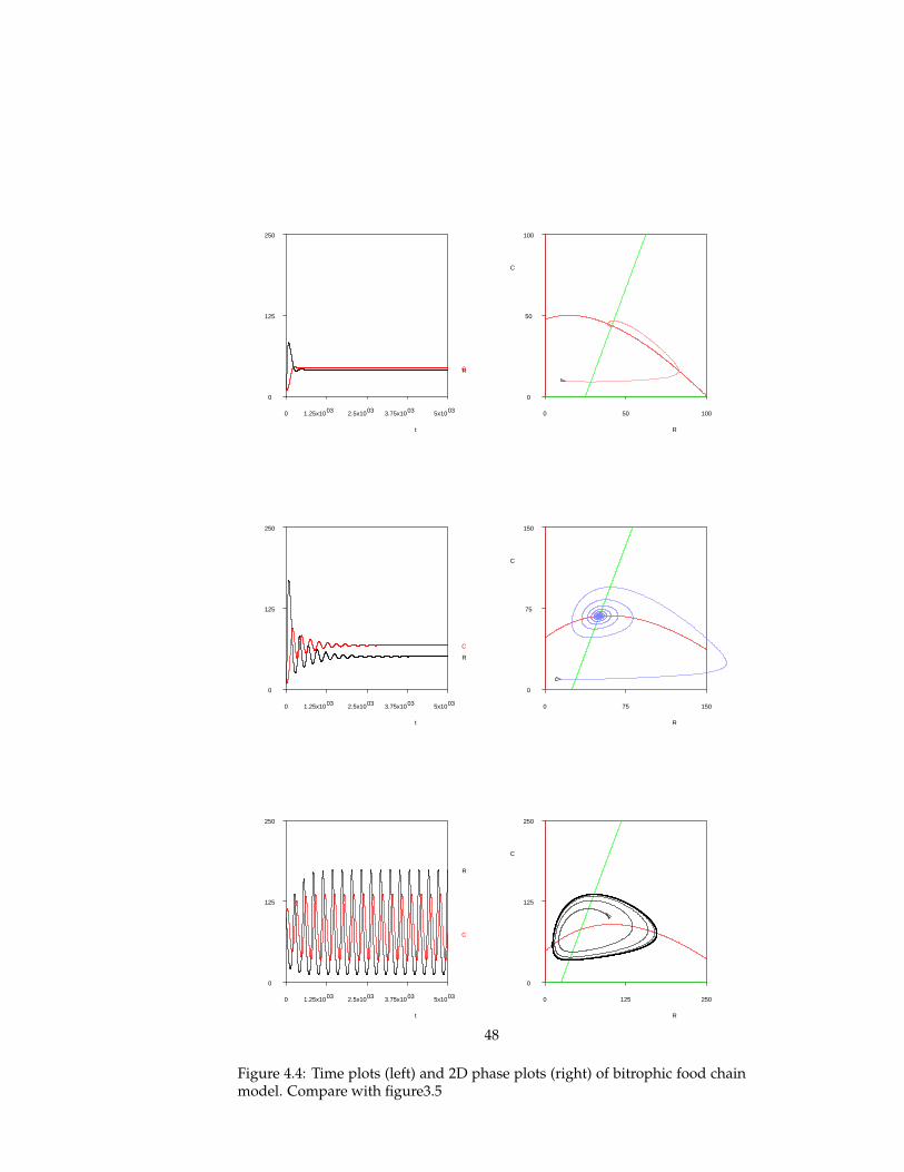
R

250

125

0

035x1003

C

3.75x10032.5x10031.25x100

t

50

0

C

100500

R

100

R

250

125

0

035x1003

C

3.75x10032.5x10031.25x100

t

75

0

C

150750

R

150

R

250

125

0

035x1003

C

3.75x10032.5x10031.25x100

t

125

0

C

2501250

R

250

Figure 4.4: Time plots (left) and 2D phase plots (right) of bitrophic food chainmodel. Compare with figure3.5

48

The dynamics observed in these simulations can now be understood ontheoretical grounds. To do this, we take theoretical model in 4.5 and fill it init with reasonable estimates of the parameters. These estimates are the resultsof curve fitting of the functional dependencies. We can now change the pa-rameter in the theoretical model that corresponds to the changes in simulationparameters across the various runs, in this case the carrying capacity K, andobserve what happens to the behaviour of the model.

Figure 4.4 shows three numerical runs for different values of K. As canbe expected, increasing the carrying capacity does not affect the consumernullcline, since this parameter does not occur in equation 4.6. The truncatedparabola describing the resource nullcline does change and expands to theright, since the logistic self-limitation of this population is decreased.

Comparing these results with the emergent population dynamics from thesimulation model in figure 3.2.1 on page 32. This confirms the applicability ofthis theoretical model to our simulation model, and shows why the simulatedbitrophic food chain is destabilized through enrichment.

Although the simulations were carried out in a way as to allow mean-ingful theoretical analysis, by tuning down spatial heterogeneity (by defin-ing placement and carrying capacity globally), some notable differences in thebehaviour of both models remain. Whereas the numerical solution shows afixed point equilibrium for K = 100 (top row panels), the simulation modelshows something that is more appropriately called a fixed cloud equilibrium.The simulated system continues to move around the equilibrium, because it ispushed out of the steady state by random fluctuations. Likewise, the situationfor K = 200 (middle row panels), shows damping oscillations in the numericalcase. The simulation model also shows damping oscillations towards a stablefixed point (or cloud), but when the system moves toward this equilibrium, itstarts to show limit cycle behaviour with small amplitude, indicating the pres-ence of an unstable equilibrium.

These differences can be attributed to the fact that the theoretical model pre-sented here is ’ideal’ in the sense that it assumes (1) infinite population num-bers and (2) deterministic interactions and events. The simulation model, bycontrast, deals with rather small populations and involves many stochastic orrandom events. Moreover, the theoretical models averages over differencesbetween individuals by using state variables pitched at the population level.Although this seems justified by the fact that all simulated individuals are infact identical, differences in consumption and reproduction rates between indi-viduals do occur in the simulations. These fitness-affecting differences are dueto differences in spatial location of individuals (e.g. by being born in an areawith high or low resource density), and are only limited due to the fact spatialhomogeneity was tuned down. When space is left free to organise itself, andthe environment for consumers becomes more structured or heterogeneous,lumping individuals in population averages becomes increasingly dangerous,and the applicability of these theoretical mini-model is undermined.

Fortunately, many interesting phenomena remain to be investigated us-ing the simulation model, even in the case of an approximately homogeneous

49

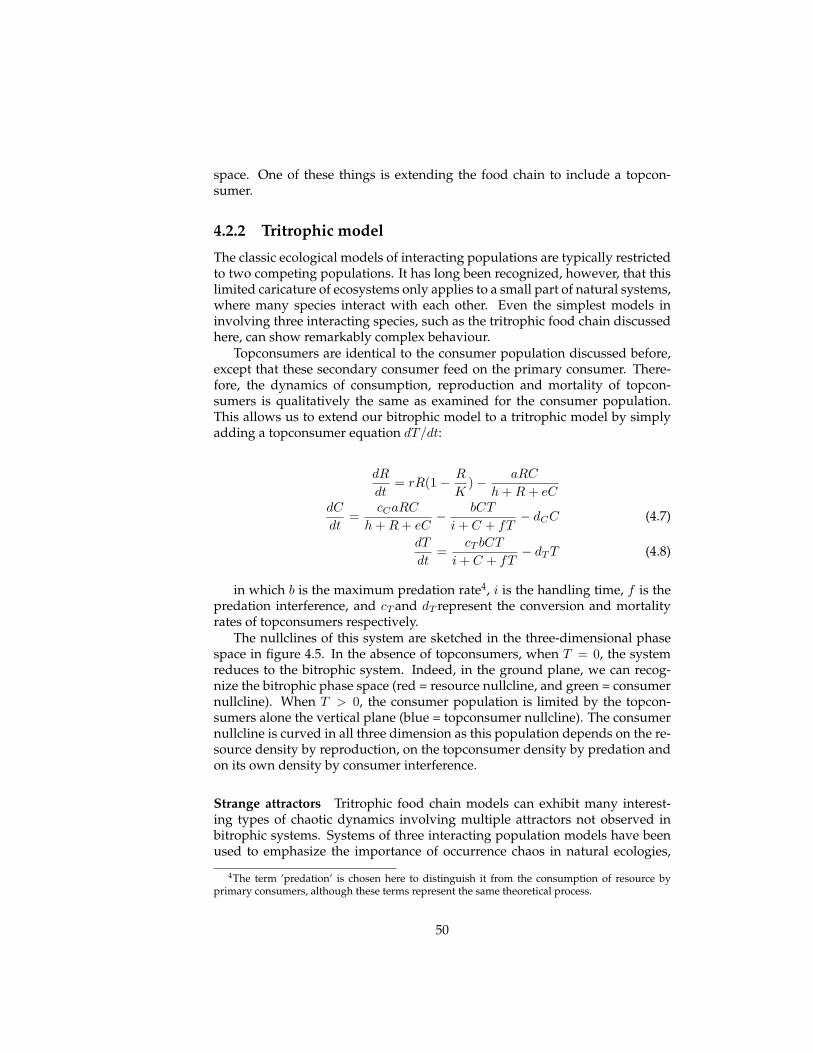
space. One of these things is extending the food chain to include a topcon-sumer.

4.2.2 Tritrophic model

The classic ecological models of interacting populations are typically restrictedto two competing populations. It has long been recognized, however, that thislimited caricature of ecosystems only applies to a small part of natural systems,where many species interact with each other. Even the simplest models ininvolving three interacting species, such as the tritrophic food chain discussedhere, can show remarkably complex behaviour.

Topconsumers are identical to the consumer population discussed before,except that these secondary consumer feed on the primary consumer. There-fore, the dynamics of consumption, reproduction and mortality of topcon-sumers is qualitatively the same as examined for the consumer population.This allows us to extend our bitrophic model to a tritrophic model by simplyadding a topconsumer equation dT/dt:

dR

dt= rR(1− R

K)− aRC

h + R + eCdC

dt=

cCaRC

h + R + eC− bCT

i + C + fT− dCC (4.7)

dT

dt=

cT bCT

i + C + fT− dT T (4.8)

in which b is the maximum predation rate4, i is the handling time, f is thepredation interference, and cT and dT represent the conversion and mortalityrates of topconsumers respectively.

The nullclines of this system are sketched in the three-dimensional phasespace in figure 4.5. In the absence of topconsumers, when T = 0, the systemreduces to the bitrophic system. Indeed, in the ground plane, we can recog-nize the bitrophic phase space (red = resource nullcline, and green = consumernullcline). When T > 0, the consumer population is limited by the topcon-sumers alone the vertical plane (blue = topconsumer nullcline). The consumernullcline is curved in all three dimension as this population depends on the re-source density by reproduction, on the topconsumer density by predation andon its own density by consumer interference.

Strange attractors Tritrophic food chain models can exhibit many interest-ing types of chaotic dynamics involving multiple attractors not observed inbitrophic systems. Systems of three interacting population models have beenused to emphasize the importance of occurrence chaos in natural ecologies,

4The term ’predation’ is chosen here to distinguish it from the consumption of resource byprimary consumers, although these terms represent the same theoretical process.

50

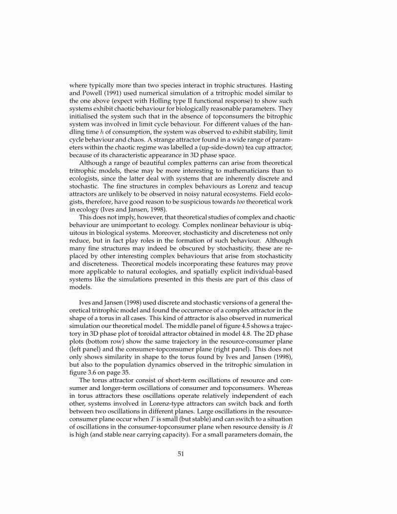
where typically more than two species interact in trophic structures. Hastingand Powell (1991) used numerical simulation of a tritrophic model similar tothe one above (expect with Holling type II functional response) to show suchsystems exhibit chaotic behaviour for biologically reasonable parameters. Theyinitialised the system such that in the absence of topconsumers the bitrophicsystem was involved in limit cycle behaviour. For different values of the han-dling time h of consumption, the system was observed to exhibit stability, limitcycle behaviour and chaos. A strange attractor found in a wide range of param-eters within the chaotic regime was labelled a (up-side-down) tea cup attractor,because of its characteristic appearance in 3D phase space.

Although a range of beautiful complex patterns can arise from theoreticaltritrophic models, these may be more interesting to mathematicians than toecologists, since the latter deal with systems that are inherently discrete andstochastic. The fine structures in complex behaviours as Lorenz and teacupattractors are unlikely to be observed in noisy natural ecosystems. Field ecolo-gists, therefore, have good reason to be suspicious towards too theoretical workin ecology (Ives and Jansen, 1998).

This does not imply, however, that theoretical studies of complex and chaoticbehaviour are unimportant to ecology. Complex nonlinear behaviour is ubiq-uitous in biological systems. Moreover, stochasticity and discreteness not onlyreduce, but in fact play roles in the formation of such behaviour. Althoughmany fine structures may indeed be obscured by stochasticity, these are re-placed by other interesting complex behaviours that arise from stochasticityand discreteness. Theoretical models incorporating these features may provemore applicable to natural ecologies, and spatially explicit individual-basedsystems like the simulations presented in this thesis are part of this class ofmodels.

Ives and Jansen (1998) used discrete and stochastic versions of a general the-oretical tritrophic model and found the occurrence of a complex attractor in theshape of a torus in all cases. This kind of attractor is also observed in numericalsimulation our theoretical model. The middle panel of figure 4.5 shows a trajec-tory in 3D phase plot of toroidal attractor obtained in model 4.8. The 2D phaseplots (bottom row) show the same trajectory in the resource-consumer plane(left panel) and the consumer-topconsumer plane (right panel). This does notonly shows similarity in shape to the torus found by Ives and Jansen (1998),but also to the population dynamics observed in the tritrophic simulation infigure 3.6 on page 35.

The torus attractor consist of short-term oscillations of resource and con-sumer and longer-term oscillations of consumer and topconsumers. Whereasin torus attractors these oscillations operate relatively independent of eachother, systems involved in Lorenz-type attractors can switch back and forthbetween two oscillations in different planes. Large oscillations in the resource-consumer plane occur when T is small (but stable) and can switch to a situationof oscillations in the consumer-topconsumer plane when resource density is Ris high (and stable near carrying capacity). For a small parameters domain, the

51

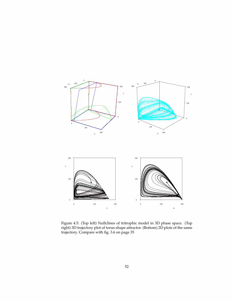
0

125

C

0

125

T

250300

0

150R

250

0

125

0

125

250

T

300

150R

0

C250

125

0

T

2501250

C

250

125

0

C

3001500

R

250

Figure 4.5: (Top left) Nullclines of tritrophic model in 3D phase space. (Topright) 3D trajectory plot of torus-shape attractor. (Bottom) 2D plots of the sametrajectory. Compare with fig. 3.6 on page 35

52

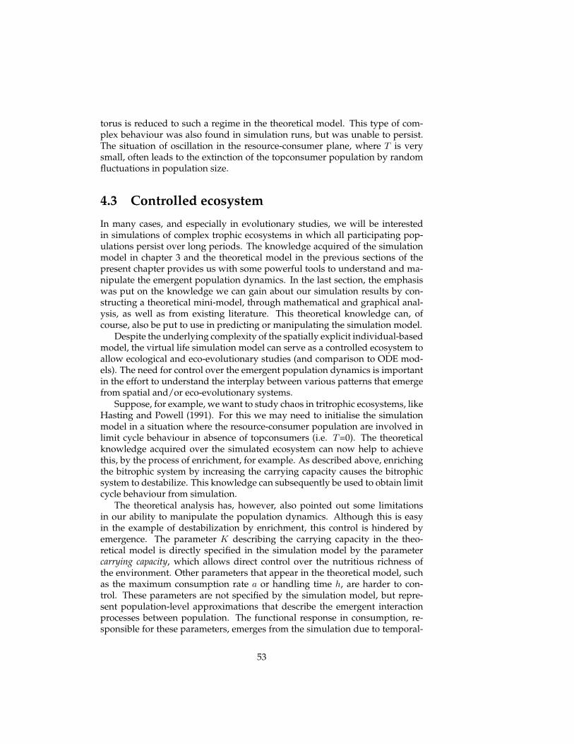
torus is reduced to such a regime in the theoretical model. This type of com-plex behaviour was also found in simulation runs, but was unable to persist.The situation of oscillation in the resource-consumer plane, where T is verysmall, often leads to the extinction of the topconsumer population by randomfluctuations in population size.

4.3 Controlled ecosystem

In many cases, and especially in evolutionary studies, we will be interestedin simulations of complex trophic ecosystems in which all participating pop-ulations persist over long periods. The knowledge acquired of the simulationmodel in chapter 3 and the theoretical model in the previous sections of thepresent chapter provides us with some powerful tools to understand and ma-nipulate the emergent population dynamics. In the last section, the emphasiswas put on the knowledge we can gain about our simulation results by con-structing a theoretical mini-model, through mathematical and graphical anal-ysis, as well as from existing literature. This theoretical knowledge can, ofcourse, also be put to use in predicting or manipulating the simulation model.

Despite the underlying complexity of the spatially explicit individual-basedmodel, the virtual life simulation model can serve as a controlled ecosystem toallow ecological and eco-evolutionary studies (and comparison to ODE mod-els). The need for control over the emergent population dynamics is importantin the effort to understand the interplay between various patterns that emergefrom spatial and/or eco-evolutionary systems.

Suppose, for example, we want to study chaos in tritrophic ecosystems, likeHasting and Powell (1991). For this we may need to initialise the simulationmodel in a situation where the resource-consumer population are involved inlimit cycle behaviour in absence of topconsumers (i.e. T=0). The theoreticalknowledge acquired over the simulated ecosystem can now help to achievethis, by the process of enrichment, for example. As described above, enrichingthe bitrophic system by increasing the carrying capacity causes the bitrophicsystem to destabilize. This knowledge can subsequently be used to obtain limitcycle behaviour from simulation.

The theoretical analysis has, however, also pointed out some limitationsin our ability to manipulate the population dynamics. Although this is easyin the example of destabilization by enrichment, this control is hindered byemergence. The parameter K describing the carrying capacity in the theo-retical model is directly specified in the simulation model by the parametercarrying capacity, which allows direct control over the nutritious richness ofthe environment. Other parameters that appear in the theoretical model, suchas the maximum consumption rate a or handling time h, are harder to con-trol. These parameters are not specified by the simulation model, but repre-sent population-level approximations that describe the emergent interactionprocesses between population. The functional response in consumption, re-sponsible for these parameters, emerges from the simulation due to temporal-

53

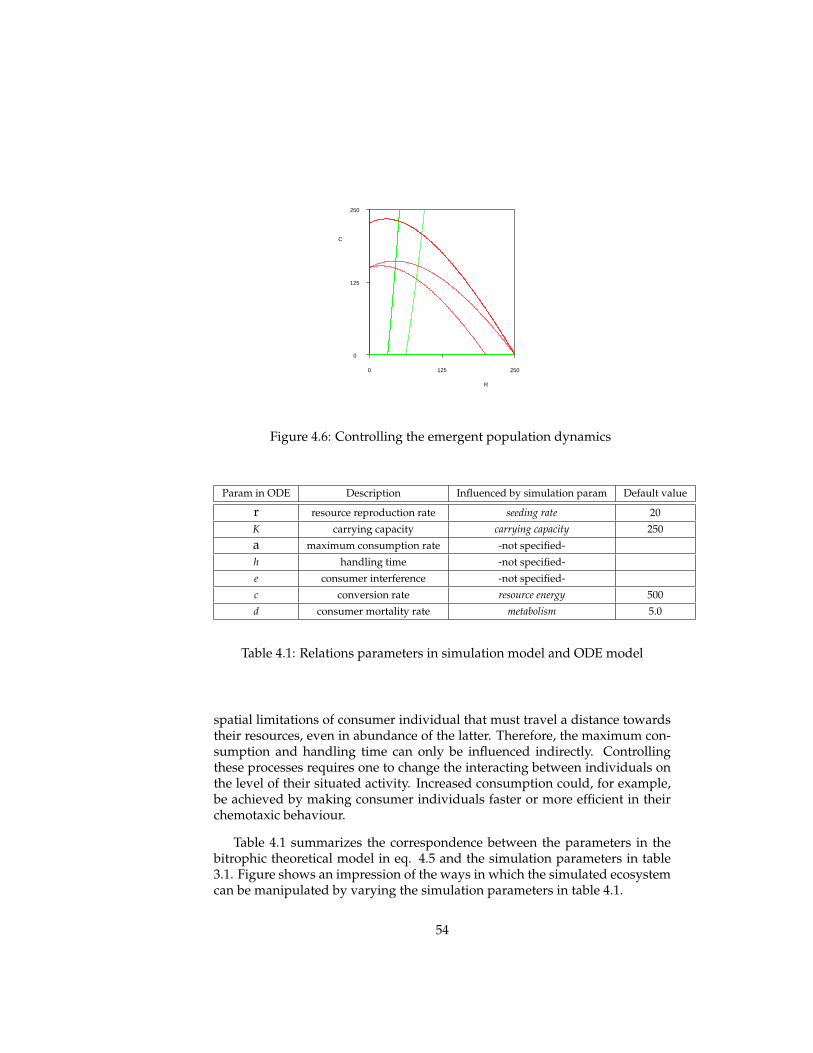
125

0

C

2501250

R

250

Figure 4.6: Controlling the emergent population dynamics

Param in ODE Description Influenced by simulation param Default value

r resource reproduction rate seeding rate 20

K carrying capacity carrying capacity 250

a maximum consumption rate -not specified-

h handling time -not specified-

e consumer interference -not specified-

c conversion rate resource energy 500

d consumer mortality rate metabolism 5.0

Table 4.1: Relations parameters in simulation model and ODE model

spatial limitations of consumer individual that must travel a distance towardstheir resources, even in abundance of the latter. Therefore, the maximum con-sumption and handling time can only be influenced indirectly. Controllingthese processes requires one to change the interacting between individuals onthe level of their situated activity. Increased consumption could, for example,be achieved by making consumer individuals faster or more efficient in theirchemotaxic behaviour.

Table 4.1 summarizes the correspondence between the parameters in thebitrophic theoretical model in eq. 4.5 and the simulation parameters in table3.1. Figure shows an impression of the ways in which the simulated ecosystemcan be manipulated by varying the simulation parameters in table 4.1.

54

4.4 Conclusions

In this chapter, the ecological interactions observed in resource-consumer in-teractions were analysed in terms of population-level variables to constructtheoretical ecological mini-models. These model enable us to understand thepopulation dynamics that emerge from interaction between simulated indi-viduals. The simulation results of the previous chapter could be interpreted interms of enrichment in the bitrophic case and a torus attractor in the tritrophicsystem. This theoretical modelling also enables us to control the emergent pop-ulation dynamics, as was shown in the last section.

55

Chapter 5

Evolutionary experiments

So far, we have examined the virtual life simulation model (in chapter 3) andhave developed analytical models to understand the ecological interactionsthat the simulations give rise to (in chapter 4). In this chapter, evolution isincorporated in the simulation model by introducing variation among individ-uals. Individuals of evolving populations are specified with inheritable andmutable traits that affect their fitness (henceforth called phenotypes) whichcauses differential reproduction. The evolutionary dynamics that emerge fromthese eco-evolutionary systems are analysed in terms of the ecological frame-work developed in the previous chapter.

A series of three eco-evolutionary experiments is presented that addressesseveral fundamental biological problems and processes that are considered tobe important to explain major transitions and complexification in evolution.Moreover, these experiments aim to illustrate the methods of ecological analy-sis and examplify the use of direct and indirect explanatory models.

The first experiment models the evolution of the reproductive efficiencyof a consumer population. This causes over-exploitation of their common re-sources which results in the extinction of the consumer population. This pro-cess is known as the (evolutionary) “tradegy of the commons” (Hardin, 1968).The second experiment models coevolution in a predator-prey ecosystem. Thisresults in the emergence of an evolutionary arms race (Dawkins and Krebs,1979) that displays red queen dynamics (van Valen, 1973). The third experi-ment is similar to the first with the exception that here spatial self-structuringof resources and consumers is allowed. This causes the formation of spatio-phenotypic consumer groups causes reproductive restraint, which prevents theconsumer population to fall victim to the “tragedy of the commons” through aprocess of group selection (Wilson, 1975; Wilson and Sober, 1994).

The applicability of ODE models to analyse these evolutionary processes islimited. The assumptions in ODE models that the populations consist of iden-tical individuals and that their spatial distributions is homogeneous are bothlifted in the experiments in this chapter. Therefore, the ODE models cannot

56

accurately model the ecological interaction of the simulation model. How-ever, they can still serve as a theoretical framework in which to understandthese ecological interactions. Moreover, they can serve to shows the differ-ences in evolutionary dynamics and outcome between the ODE model and theindividual-based simulation model.

In order to allow the ODE model to serve as a meaningful framework, evenwhen confronted with these differences, the ’genetics’ involved in the evolu-tionary experiments is kept extremely simple. Individuals carry only a sin-gle gene that directly affects it behaviour (phenotype) without development orlearning. Such phenotypes are single real values that directly control consump-tion rates or reproduction efficiencies. This means that there are clear relationsbetween the evolving phenotypes in the simulation models and the parame-ters in the ODE models. Therefore, changes in the (population averages of)phenotypes can be interpreted as changes in one of the parameters in the ODEmodel.

Explanations of observed evolutionary dynamics differs from standard thepractice in artificial life. Instead of relating the observed emergent phenomenonback to specifications in the simulation model directly, the emergent evolu-tionary dynamics are explained indirectly by relating them to other emergentpatterns (i.e. population dynamics and spatial self-structuring). The structureof the explanatory model grows more intricate as the interplay between theseemergent patterns grows increasing complex over the three experiments pre-sented below. This results in explanations of evolutionary phenomena that arebased on generic biological processes (evolution, population dynamics, andspatial structure) and are less dependent on the specific details of the simula-tion models.

5.1 Evolution

5.1.1 Introduction

The first simulation implements a simple eco-evolutionary system. It is simi-lar to the ecological experiments in chapter 3, except that it includes variationamong consumer individuals. This variation serves as a substrate for naturalselection and alters the phenotypic configuration of the population by differ-ential reproduction.

In this experiment, evolution can alter the energy that a consumer obtainsfrom eating a resource. Natural selection favours consumers that gain moreenergy over the ones gaining less energy from resources, since the former re-produce more often. This leads to an overall increase of population size ofthe consumer population, ecological instability and eventually extinction ofconsumers. The evolutionary maximization of individual gain causes an over-exploitation of common resources as the “selfish” consumers fall victim to the“tradegy of the commons”(Hardin, 1968).

57

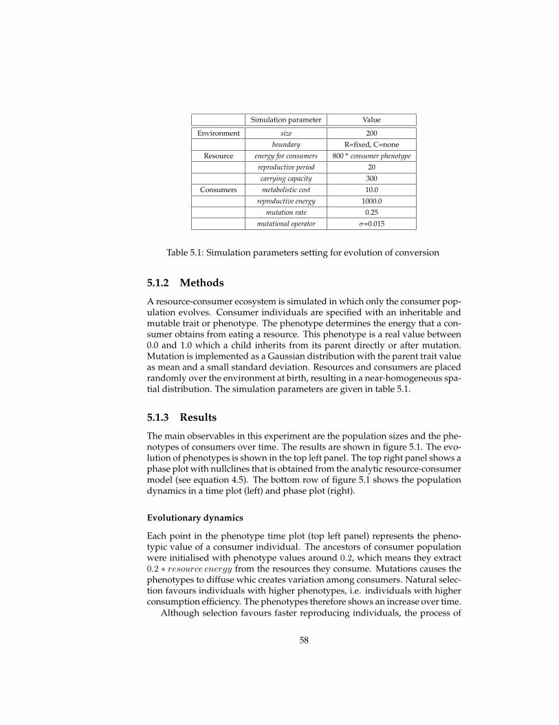
Simulation parameter Value

Environment size 200

boundary R=fixed, C=none

Resource energy for consumers 800 * consumer phenotypereproductive period 20

carrying capacity 300

Consumers metabolistic cost 10.0

reproductive energy 1000.0

mutation rate 0.25

mutational operator σ=0.015

Table 5.1: Simulation parameters setting for evolution of conversion

5.1.2 Methods

A resource-consumer ecosystem is simulated in which only the consumer pop-ulation evolves. Consumer individuals are specified with an inheritable andmutable trait or phenotype. The phenotype determines the energy that a con-sumer obtains from eating a resource. This phenotype is a real value between0.0 and 1.0 which a child inherits from its parent directly or after mutation.Mutation is implemented as a Gaussian distribution with the parent trait valueas mean and a small standard deviation. Resources and consumers are placedrandomly over the environment at birth, resulting in a near-homogeneous spa-tial distribution. The simulation parameters are given in table 5.1.

5.1.3 Results

The main observables in this experiment are the population sizes and the phe-notypes of consumers over time. The results are shown in figure 5.1. The evo-lution of phenotypes is shown in the top left panel. The top right panel shows aphase plot with nullclines that is obtained from the analytic resource-consumermodel (see equation 4.5). The bottom row of figure 5.1 shows the populationdynamics in a time plot (left) and phase plot (right).

Evolutionary dynamics

Each point in the phenotype time plot (top left panel) represents the pheno-typic value of a consumer individual. The ancestors of consumer populationwere initialised with phenotype values around 0.2, which means they extract0.2 ∗ resource energy from the resources they consume. Mutations causes thephenotypes to diffuse whic creates variation among consumers. Natural selec-tion favours individuals with higher phenotypes, i.e. individuals with higherconsumption efficiency. The phenotypes therefore shows an increase over time.

Although selection favours faster reproducing individuals, the process of

58

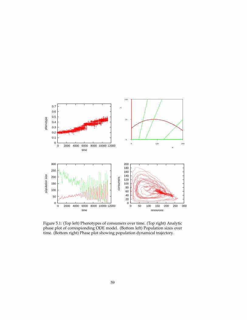
0

0.1

0.2

0.3

0.4

0.5

0.6

0.7

0 2000 4000 6000 8000 10000 12000

phen

otyp

e

time

75

0

C

2501250

R

150

0

50

100

150

200

250

300

0 2000 4000 6000 8000 10000 12000

popu

latio

n si

ze

time

0 20 40 60 80

100 120 140 160 180 200

0 50 100 150 200 250 300

cons

umer

s

resources

Figure 5.1: (Top left) Phenotypes of consumers over time. (Top right) Analyticphase plot of correspionding ODE model. (Bottom left) Population sizes overtime. (Bottom right) Phase plot showing population dynamical trajectory.

59

removal of suboptimal phenotypes from the population is slower than thereproduction of the individuals carrying suboptimal phenotypes. Relativelyslow reproducing individuals can therefore remain present in the population,and optimal phenotypes do not fix in the population (i.e. no complete domi-nance). Instead, the time plot of phenotypes shows the evolution of “clouds” ofclosely related phenotypes, known as quasispecies in molecular evolutionarybiology (Eigen and Schuster, 1979; Eigen, 1971).

The increase of phenotypes does not proceed entirely smoothly. Most no-tably, a sudden increase is observed after 6000 time steps. Just before this point,the number of different phenotypes in the population increases and the start ofa speciation event is observed (single quasispecies cloud breaking up into twoclouds). The abrupt phenotypic increase is due to selection of the upper qua-sispecies at the expense of the lower part. Interestingly, these events coincidewith changes in the population dynamics in the bottom left plot.

After approximately 11500 time steps, evolution comes to a halt when theconsumers have phenotypic values around 0.45. To see why evolution is inter-rupted at these values, instead of evolving towards the maximum of 1.0, thepopulation dynamics must be taken into account.

Population dynamics

The population dynamics (bottom left panel) shows an increasing instabilityof the ecological dynamics. Initially, the population sizes settle at a relativelystable equilibrium (only perturbed by stochasticity). During the first phase,the consumer population slowly increases in size at the expense of the re-source population. In the phase plot (bttom right panel), this is reflected bythe dark region of the trajectory. After 5500 timesteps, regular oscillations startto emerge. The amplitude of these oscillations increases over time which isshown in the phase plot as limit cycles. Eventually, this instability leads to theextinction of the resource populations, followed by the consumers that dependon them.

The increasing instability of the population dynamics can only be attributedto the phenotypic character of the consumer population (because nothing elsechanges) and visual inspection of both time plots (left panels) shows strongcorrelation. As the phenotypes of the consumers increase, the ecosystem showincreasing instability. Consumers evolve towards their own extinction.

Eco-evolutionary analysis

The observed dynamics can be understood by relating the simulated eco-evolutionarysystem to the analytical resource-consumer model:

60

dR

dt= rR(1− R

K)− aRC

h + R + eCdC

dt=

caRC

h + R + eC− dC (5.1)

which is equal to model 4.5 as examined in more detail on page 46.From the simulation model, we know that consumer reproduction fully

depends on energy levels, and that energy levels depends on consumption(energy gain) and metabolism (energy loss). The phenotype determines theamount of energy that a consumer gains from eating a resource. The energyrequired for reproduction and the energy lossed by metabolism is equal forall consumers, independent of their phenotypes. Therefore, an increase in en-ergy gain causes an increase in the conversion of consumed resource into newoffspring.

In the analytical model, this conversion is captured in the biomass conver-sion coefficient c. Changes in the population average of the consumer pheno-types in simulation can be interpreted as a change of this conversion parameterin the analytical model. Since evolution of the consumers adapts their biomassconversion parameter, we can study the observed population dynamics by ex-amining the effect of changes of c in the ODE model.

To do this, we sketch the nullclines of the theoretical model with reasonableestimates of the parameters, for various values of the conversion parameter c.This is shown in the phase plot (top right panel), where the green consumernullcline is drawn for three value of c. The values roughly correspond to pop-ulation average of phenotypes in the first, middle and last periods in the evo-lutionary run.

The rightmost consumer nullcline corresponds to the initial period in thesimulation. Stability analysis shows that the equilibrium in this configurationis stable (i.e. see panel (d) in fig. 4.3). As the consumer nullcline moves to theleft as a result of an increase in c, the equilibria become unstable. Trajectoriesin phase space of the situation with the middle nullcline show limit cycles.The amplitudes of these limit cycles grows larger as the conversion parameterincreases. Eventually, the amplitude of the limit cycles becomes too large andboth populations go extinct.

The ecological interactions put a constraint on the evolvability of the biomassconversion. High conversion parameter values (e.g. greater than 0.5) are notevolvable in this ecosystem, because such values are not ecologically viable.

Tragedy of the commons

Evolution, the process of mutation and selective reproduction, acts to increasethe fitness of individuals. This causes the growth of the consumer population,at the expense of the resource population. All consumers share a common re-source pool in which the resources are renewed at a limited rate. The consumerpopulation evolves to increase its reproduction rate, but the reproduction of

61

resources remains constant. This leads to an overexploitation of resources, fol-lowed by an explosion of the consumer population. As this offspring has lit-tle or no resources left to eat, because the resource population do not have achance to grow back, the consumer population goes extinct. The consumerpopulation has fallen victim to the “tradegy of the commons” (Hardin, 1968).

5.1.4 Conclusion

The results of this eco-evolutionary experiment illustrate the relation betweenevolutionary and population dynamics. Natural selection favours consumerindividuals with higher energy gain, because they have more offspring on av-erage, and therefore out-compete their less efficient conspecifics. The energygain of the consumer population also has major influence on the populationdynamics. In the ODE model, the evolution of this trait could be interpreted aschange in the biomass conversion parameter c. Varying this parameter enablesus to understand the observed population dynamics as well as understand theecological constraints on the evolvability of conversion values. The evolution-ary dynamics are constrained by the ecological principle of the “tragedy of thecommons”.

This tragedy seems to suggest that cooperation and altruism cannot evolvebecause natural selection always favours selfish individuals. And indeed, thisis predicted from the analytical model, and was confirmed by the simulationmodel. This results does, however, depend on the homogeneous spatial dis-tubition that is implicit in the ODE model and was explicitly modelled in thesimulation model. We will return to this point in section 5.3, in which similarexperiments are conducted in a system that allows spatial heterogeneity. First,however, a coevolutionary simulation is presented in which an evolutionaryarms race is observed that exhibits red queen dynamics.

5.2 Coevolution1

5.2.1 Introduction

Coevolution of predators and prey is often understood in terms of evolution-ary arms races. These arms races occur because predators and prey do not onlycompete on a behavioral scale, but also on an evolutionary scale (Dawkins andKrebs, 1979). Arms races between coevolving populations are considered as animportant source of evolutionary complexification. However, arms races donot necessarily cause populations to be better adapted to their environment.Van Valen (1973) noticed that populations with long histories go extinct withthe same frequency as populations with relatively short evolutionary histories.This indicates that the coevolutionary coupling between populations do not

1A modified version of this section has been submitted to GECCO 2006 conference as “Redqueen dynamics in predator-prey ecosystem”, W. de Back, M. Wiering, E. de Jong.

62

cause them to be better adapted to their environment, because this environ-ment is evolving with them. Van Valen (1973) adopted the term ’red queen’ todenote the fact that in coevolution, populations evolve only to maintain insteadof improve their fitness.

Coevolutionary systems can be contracting, expanding, or involved in redqueen dynamics, depending on the lag load. The lag load describes the reduc-tion of mean population fitness due to the average trait of a population differ-ing form its optimal value. That is, it is the distance a population lags behind,realtive to its evolving antagonist. When the lag load of a population increasesover time, it is losing relative to its antagonist, which (by contraction) can leadto extinction. The antagonist, in this case, has a decreasing lag load and willgrow (expand) in population size. Both coevolutionary modes are not sustain-able as they lead to the extinction of one of the competitors, unless these modesalternate. Red queen dynamics is a steady state in the evolutionary dynamicswhich occurs when both populations have a positive but constant lag load. Inthis case, both populations continually adapt to each other, while remaining atthe same fitness.

The simulation results show the simultaneous emergence of patterns inpopulation and evolutionary dynamics. We do not merely explain these dy-namics as the emergent outcome of interaction between individuals, but ex-plain these two patterns by relating them to each other, using the populationdynamical model. In this fashion, it is established that the coevolving ecosys-tem is involved in an evolutionary arms race. After a short asymmetric period,in which the relative fitnesses (and lag load) changes, the arms race settles ina relatively steady state in which both populations do not receive any fitnessbenefits. That is, the arms race settles in a red queen dynamics.

5.2.2 Methods

A resource-consumer (or predator-prey) ecosystem is used in which both pop-ulations evolve. In contrast to the previous experiment, here, both preda-tors and prey individuals are specified with a phenotype. The coevolutionarymodel that is used in this experiment here is adopted from van der Laan andHogeweg (1995) and its spatial extension in Savill and Hogeweg (1997).

Phenotypes

This phenotype is a natural value between 0 and 100. When a predator and aprey interact (collide), the difference between the two phenotypes determinesthe probability of predation (i.e. energy transfer) according to

p(predation)∝a = exp(−(phenoR − phenoC

σ)2) (5.2)

which defines a Gaussian distribution, where the standard deviation σ canbe interpreted as the specialism or generalism of the predators (kept constant inthese experiments). Predation probabilities are highest (1.0) for predator-prey

63

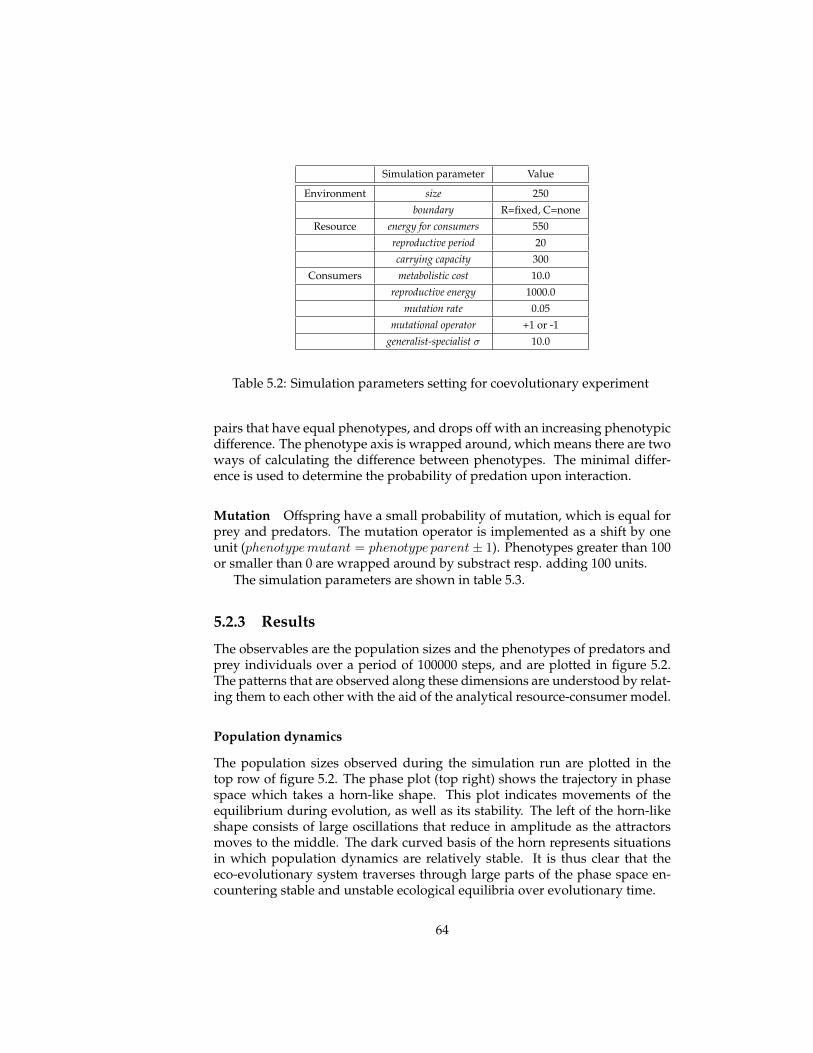
Simulation parameter Value

Environment size 250

boundary R=fixed, C=none

Resource energy for consumers 550

reproductive period 20

carrying capacity 300

Consumers metabolistic cost 10.0

reproductive energy 1000.0

mutation rate 0.05

mutational operator +1 or -1

generalist-specialist σ 10.0

Table 5.2: Simulation parameters setting for coevolutionary experiment

pairs that have equal phenotypes, and drops off with an increasing phenotypicdifference. The phenotype axis is wrapped around, which means there are twoways of calculating the difference between phenotypes. The minimal differ-ence is used to determine the probability of predation upon interaction.

Mutation Offspring have a small probability of mutation, which is equal forprey and predators. The mutation operator is implemented as a shift by oneunit (phenotypemutant = phenotype parent± 1). Phenotypes greater than 100or smaller than 0 are wrapped around by substract resp. adding 100 units.

The simulation parameters are shown in table 5.3.

5.2.3 Results

The observables are the population sizes and the phenotypes of predators andprey individuals over a period of 100000 steps, and are plotted in figure 5.2.The patterns that are observed along these dimensions are understood by relat-ing them to each other with the aid of the analytical resource-consumer model.

Population dynamics

The population sizes observed during the simulation run are plotted in thetop row of figure 5.2. The phase plot (top right) shows the trajectory in phasespace which takes a horn-like shape. This plot indicates movements of theequilibrium during evolution, as well as its stability. The left of the horn-likeshape consists of large oscillations that reduce in amplitude as the attractorsmoves to the middle. The dark curved basis of the horn represents situationsin which population dynamics are relatively stable. It is thus clear that theeco-evolutionary system traverses through large parts of the phase space en-countering stable and unstable ecological equilibria over evolutionary time.

64

In contrast to the previous experiment, this does not occur in a unidirec-tional manner (as in the previous evolutionary experiment), as is clear fromthe time plot (top left in fig. 5.2). This plot shows alternating periods withqualitatively different behaviours: periods of instability characterised by oscil-lations, relatively stable periods, and near-extinction events of consumers. Thesystem, for example, shows oscillatory behaviour in the initial phase, and aftera period of relative stability, oscillations are re-encountered after some 75000time steps. The coevolving system is thus able to move back and forth throughecological phase space.

To understand why this is possible, the analytical resource-consumer (orpredator-prey) model is useful again:

dR

dt= rR(1− R

K)− aRC

h + R + eCdC

dt=

caRC

h + R + eC− dC (5.3)

The difference between phenotypes determine the probability of actual pre-dation on interaction between a predator and a prey (eq. 5.2). The more similarthe phenotypes of interacting antagonist, the higher the probability of success-ful predation, thus increasing the predation rate. The movements of the equi-librium through phase space can thus be interpreted as evolutionary changesin the maximum predation rate a.

The bottom right plot in figure 5.2 shows an graphical construction of theanalytical model in eq. 5.3. Nullclines are sketched for various values of themaximum predation rate a, and the (in)stability of the various equilibria areindicated by open (unstable) and closed (stable) boxes. The equilibria moveto the right as the maximum predation rate decreases. By comparison of both(experimental and analytical) phase plots, the parts of the phase space throughwhich the system traverses can be understood as changes in maximum preda-tion rate a. It does not, however, enable us to appreciate why the equilibria canmove back and forth through phase space without extinction. To understandthis, the evolutionary dynamics must be examined in more detail.

Evolutionary arms race

The evolution of phenotypes of predators (red) and prey (green) are depictedin the bottom left plot in figure 5.2. The double stripes show the predators chas-ing the prey (and prey evading the predator) phenotypes phenotypes throughphenotype space (with wrap-around boundaries). The predators chase theirprey in real space over ecological time, as well as in phenotype space over evo-lutionary time. They are bound in an evolutionary arms race.

From eq. 5.2 we know that predation rates are determined by the differencesbetween the phenotypes of predators and prey. The solid line in the plot rep-resents the population average phenotypic difference between the predators

65

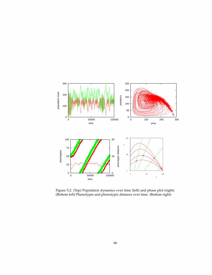
0

100

200

300

0 50000 100000

popu

latio

n si

zes

time

0

50

100

150

200

250

0 100 200 300pr

edat

ors

prey

0

25

50

75

100

0 50000 100000 0

25

50

phen

otyp

es

phen

otyp

ic d

ista

nce

time

125

0

C

3001500

R

250

Figure 5.2: (Top) Population dynamics over time (left) and phase plot (right).(Bottom left) Phenotypes and phenotypic distance over time. (Bottom right)

66

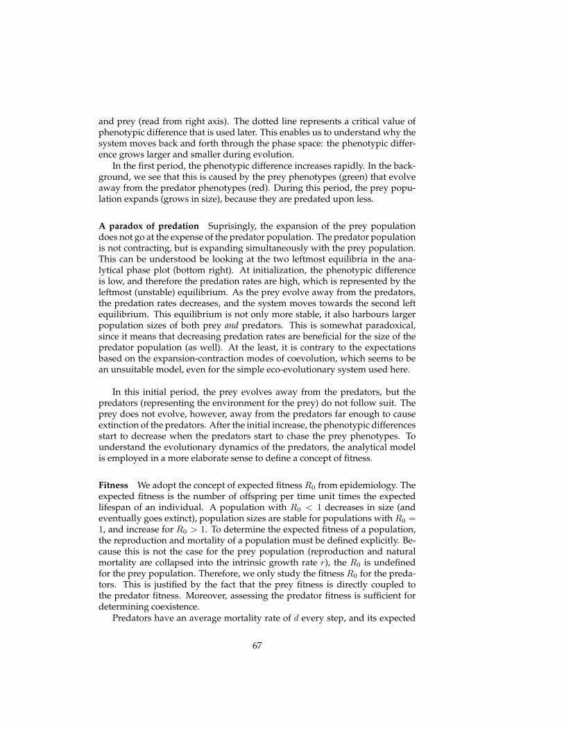
and prey (read from right axis). The dotted line represents a critical value ofphenotypic difference that is used later. This enables us to understand why thesystem moves back and forth through the phase space: the phenotypic differ-ence grows larger and smaller during evolution.

In the first period, the phenotypic difference increases rapidly. In the back-ground, we see that this is caused by the prey phenotypes (green) that evolveaway from the predator phenotypes (red). During this period, the prey popu-lation expands (grows in size), because they are predated upon less.

A paradox of predation Suprisingly, the expansion of the prey populationdoes not go at the expense of the predator population. The predator populationis not contracting, but is expanding simultaneously with the prey population.This can be understood be looking at the two leftmost equilibria in the ana-lytical phase plot (bottom right). At initialization, the phenotypic differenceis low, and therefore the predation rates are high, which is represented by theleftmost (unstable) equilibrium. As the prey evolve away from the predators,the predation rates decreases, and the system moves towards the second leftequilibrium. This equilibrium is not only more stable, it also harbours largerpopulation sizes of both prey and predators. This is somewhat paradoxical,since it means that decreasing predation rates are beneficial for the size of thepredator population (as well). At the least, it is contrary to the expectationsbased on the expansion-contraction modes of coevolution, which seems to bean unsuitable model, even for the simple eco-evolutionary system used here.

In this initial period, the prey evolves away from the predators, but thepredators (representing the environment for the prey) do not follow suit. Theprey does not evolve, however, away from the predators far enough to causeextinction of the predators. After the initial increase, the phenotypic differencesstart to decrease when the predators start to chase the prey phenotypes. Tounderstand the evolutionary dynamics of the predators, the analytical modelis employed in a more elaborate sense to define a concept of fitness.

Fitness We adopt the concept of expected fitness R0 from epidemiology. Theexpected fitness is the number of offspring per time unit times the expectedlifespan of an individual. A population with R0 < 1 decreases in size (andeventually goes extinct), population sizes are stable for populations with R0 =1, and increase for R0 > 1. To determine the expected fitness of a population,the reproduction and mortality of a population must be defined explicitly. Be-cause this is not the case for the prey population (reproduction and naturalmortality are collapsed into the intrinsic growth rate r), the R0 is undefinedfor the prey population. Therefore, we only study the fitness R0 for the preda-tors. This is justified by the fact that the prey fitness is directly coupled tothe predator fitness. Moreover, assessing the predator fitness is sufficient fordetermining coexistence.

Predators have an average mortality rate of d every step, and its expected

67

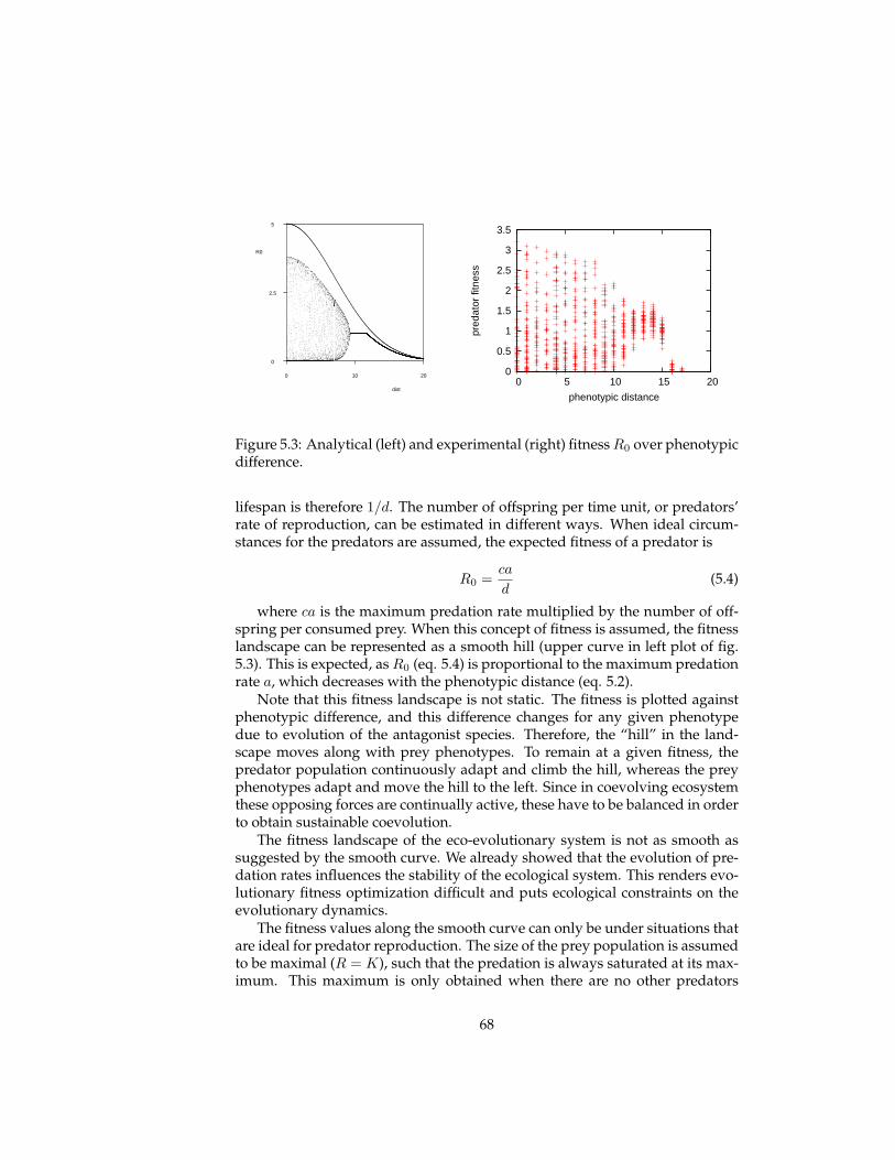
2.5

0

R0

20100

dist

5

0

0.5

1

1.5

2

2.5

3

3.5

0 5 10 15 20

pred

ator

fitn

ess

phenotypic distance

Figure 5.3: Analytical (left) and experimental (right) fitness R0 over phenotypicdifference.

lifespan is therefore 1/d. The number of offspring per time unit, or predators’rate of reproduction, can be estimated in different ways. When ideal circum-stances for the predators are assumed, the expected fitness of a predator is

R0 =ca

d(5.4)

where ca is the maximum predation rate multiplied by the number of off-spring per consumed prey. When this concept of fitness is assumed, the fitnesslandscape can be represented as a smooth hill (upper curve in left plot of fig.5.3). This is expected, as R0 (eq. 5.4) is proportional to the maximum predationrate a, which decreases with the phenotypic distance (eq. 5.2).

Note that this fitness landscape is not static. The fitness is plotted againstphenotypic difference, and this difference changes for any given phenotypedue to evolution of the antagonist species. Therefore, the “hill” in the land-scape moves along with prey phenotypes. To remain at a given fitness, thepredator population continuously adapt and climb the hill, whereas the preyphenotypes adapt and move the hill to the left. Since in coevolving ecosystemthese opposing forces are continually active, these have to be balanced in orderto obtain sustainable coevolution.

The fitness landscape of the eco-evolutionary system is not as smooth assuggested by the smooth curve. We already showed that the evolution of pre-dation rates influences the stability of the ecological system. This renders evo-lutionary fitness optimization difficult and puts ecological constraints on theevolutionary dynamics.

The fitness values along the smooth curve can only be under situations thatare ideal for predator reproduction. The size of the prey population is assumedto be maximal (R = K), such that the predation is always saturated at its max-imum. This maximum is only obtained when there are no other predators

68

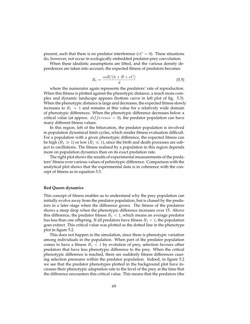
present, such that there is no predator interference (eC = 0). These situationsdo, however, not occur in ecologically embedded predator-prey coevolution.

When these idealistic assumptions are lifted, and the various density de-pendences are taken into account, the expected fitness of predators becomes

R1 =caR/(h + R + eC)

d(5.5)

where the numerator again represents the predators’ rate of reproduction.When this fitness is plotted against the phenotypic distance, a much more com-plex and dynamic landscape appears (bottom curve in left plot of fig. 5.3).When the phenotypic distance is large and decreases, the expected fitness slowlyincreases to R1 = 1 and remains at this value for a relatively wide domainof phenotypic differences. When the phenotypic difference decreases below acritical value (at approx. difference = 9), the predator population can havemany different fitness values.

In this region, left of the bifurcation, the predator population is involvedin population dynamical limit cycles, which render fitness evaluation difficult.For a population with a given phenotypic difference, the expected fitness canbe high (R1 À 1) or low (R1 ¿ 1), since the birth and death processes are sub-ject to oscillations. The fitness realised by a population in this region dependsmore on population dynamics than on its exact predation rate.

The right plot shows the results of experimental measurements of the preda-tors’ fitness over various values of pehnotypic difference. Comparison with theanalytical plot shows that the experimental data is in coherence with the con-cept of fitness as in equation 5.5.

Red Queen dynamics

This concept of fitness enables us to understand why the prey population caninitially evolve away from the predator population, but is chased by the preda-tors in a later stage when the difference grows. The fitness of the predatorsshows a steep drop when the phenotypic difference increases over 15. Abovethis difference, the predator fitness R1 < 1, which means an average predatorhas less than one offspring. If all predators have fitness R1 < 1, the populationgoes extinct. This critical value was plotted as the dotted line in the phenotypeplot in figure 5.2.

This does not happen in the simulation, since there is phenotypic variationamong individuals in the population. When part of the predator populationcomes to have a fitness R1 < 1 by evolution of prey, selection favours otherpredators that have less phenotypic difference to the prey. When the criticalphenotypic difference is reached, there are suddenly fitness differences caus-ing selection pressures within the predator population. Indeed, in figure 5.2we see that the predator phenotypes plotted in the background plot have in-creases their phenotypic adaptation rate to the level of the prey at the time thatthe difference encounters this critical value. This means that the predators (the

69

environment of the evolving prey) starts to change as fast as the prey is chang-ing.

During the rest of the simulation, the phenotypic difference remains mainlyin the region between 12 and 15, with some fluctuations. These fluctuations canbe related to the predator fitnesses in this region. In figure 5.3, we see that inthis region, the fitness landscape is fairly flat and therefore induce little selec-tive pressure. For the predators to remain in this comfortable region, their phe-notypes must evolve as quickly as the prey phenotypes. In absence of a strongselection pressure, however, the predators are likely to lag behind. When thedifference has again grown to the critical value 15, strong selection cause thepredators to catch up with the prey. This enables us to interpret the long evo-lutionary walk close to this critical difference value (fig. 5.2). Moreover, it ex-plains the alternating behaviours and reversals of movements through phasespace that were observed in the population dynamics. These reversals coincidewith the encounters with this maximum.

Although the phenotypic difference is likely to be near the critical value,since the selection pressure in the predator population is weak, so that the lagload increases until strong selection reinstalls when the critical difference isreached. This is indeed most frequently observed in the simulation. Thereis, however, also one event (observed around 75000 steps) in which the dif-ferences suddenly decreases significantly. This sudden movement is causedby the fact that a small portion of the evolving predator population that hasrapidly evolved towards the prey (possibly facilitated by the near-neutral evo-lution in region 12-15). As figure 5.3 shows, predators left of the bifurcationcan gain high fitness R1 À 1, and therefore quickly take over the predatorpopulation. This is only temporary, however, since the increased predationrate causes stronger selection pressure in the prey population which evolvesaway, as it did during the initial phase.

The two limiting mechanisms discussed above cause the evolutionary dy-namics (of the observable of phenotypic difference) to be constrained to a cer-tain parameter range in which predators and prey can coexist. The evolution-ary adaptation rates of predators and prey balances themselves, such that theenvironment of an evolving population moves as fast as it is adapting to it.This is where the red queen reigns: "Now, here, you see, it takes all the runningyou can do, to keep in the same place" Carroll (1899).

5.2.4 Conclusions

In this experiment, an eco-evolutionary simulation of predator-prey coevolu-tion was presented. The results show the emergence of an evolutionary armsrace, a paradox of predation and red queen dynamics. These processes wereexplained by relating the population and evolutionary dynamics to each otherwith the aid of an analytical predator-prey model.

70

Initially, the evolutionary arms race was assymetrical as the prey popula-tion evolves away from the predator phenotypes. During this period, a para-dox of predation is observed, as both the prey and the predator populationsexpand when predation rates decrease. This paradox was resolved by analyt-ical modelling of the evolutionary change in the maximum predation rate a.The coevolving system is able to move back and forth through phase space,dependent on the phenotypic differences. After the initial increase of this dif-ference, a decrease is observed after an encounter with the critical phenotypicdifference of 15. This reversal was explained by developing a concept of fitnessR1 and by showing that R1 < 1 for predator individuals with a phenotypicdifference geater than 15. As a result, the phenotypic difference stays in thecomfortable region between approximately 12 and 15.

The sustainability of the evolutionary arms race between predators andprey, i.e. the ecological coexistence of both populations over evolutionary time,is due to Red Queen dynamics. A lower bound of phenotypic difference causesthe prey population to evolve away from the predators, and an upper boundcauses a strong selection in the predator population towards the prey pheno-types. The Red Queen dynamics emerge as ecological constraints on the evolv-ability of the phenotypic difference.

5.3 Multi-level selection

5.3.1 Introduction

There has been a much controversy and debate about the level upon whichDarwinian selection operates. In the last decade, however, biologists haveadopted spatially explicit and individual-oriented modelling approaches whichshow the emergence of new levels of selection through spatial self-structuring(Boerlijst and Hogeweg, 1991; Johnson and Boerlijst, 2002). When the pheno-typic similarity of individuals within a self-structured patch, cluster or wave(henceforth: group) is higher than the similarity of individuals between groups,evolution can use these groups as a substrate for selection. Selection on thelevel of groups can be opposite to the direction of individual selection, andtherefore influences evolutionary dynamics (discussed in section 2.3.3).

Although group selection is accepted among biologists as a theoretical pos-sibility, many hold that its impact is too weak to be of much interest for thestudy of natural evolving ecosystems of small and viscous populations (Williams,1966). To investigate the emergence of group selection under these conditionsin our simulation model, we use a modified version of the simulation model ofthe evolution of the energy gain in section 5.1.

Consumers are again specified with an inheritable and mutable phenotypethat determines the amount of energy they extract when eating a resource.In contrast to the previous experiment, however, the spatial structure of themodel is no longer homogeneous (not well-mixed). The carrying capacity andresource placement are locally defined, which enables spatial self-structuring

71

of the resource population (see section 3.2.2). Moreover, the offspring of con-sumers are placed close to their parents, through which the spatial distributionof the consumer population becomes heterogenous as well.

This small change in the model causes qualitatively different ecologicaland evolutionary dynamics. The consumer population does not go extinct,and the phenotypes shows the evolution of reproductive restraint. The anal-ysis of the emergent evolutionary dynamics is based on studying its relationto other emergent patterns in population dynamics and spatial structure. Theemergence of spatio-phenotypic clusters results in a selection pressure betweenclusters that is opposite to the selection pressure acting upon individuals.

Although restraining reproduction is harmful to the fitness of the restrain-ing individual, it is confers an advantage to the fitness of the group it belongsto. This evolution of altruistic, in which individual-level fitness is sacrificiedfor the persistance of the population, is enabled by group selection. Group ofselfish individual fall victim to the “tragedy of the commons” leaving a popu-lation of groups of more restrained consumers.

5.3.2 Methods

The model is similar to the one described in section 5.1, with the exception thatthe resource carrying capacity and the placement of reources and consumersis now defined locally2. The spatial distribution of the consumer populationstructures itself by placing new consumers close to their parents. Since theconsumers are reactive agents that act upon their local environment, consumerin the same environment behave in similar ways (although sensory noise pre-vents agents to travel exactly the same trajectories). Therefore, small areas withrelatively high consumer populations are formed. The metabolic energy costis increased (compared to previous experiments) such that the exploration of aconsumer is limited in (life)time and space (ensuring local interaction).

Simulation parameters are shown in table 5.3.

Models

Spatial structuring of population has influence on both ecological and evolu-tionary dynamics. Our aim is to investigate the influence of spatial structur-ing on the evolutionary dynamics. Therefore, the ecological impact should bedistinguished from the evolutionary. To this end, three different models aresimulated that differ in the way individuals are placed in the environment:

Model 1 Random placement: uniform distribution over whole environment

2The local definition of resource carrying capacity and placement is here implemented as fol-lows: The environment is divided into an array of ’demes’ in which the resource populationgrowth is logistic. The carrying capacity is determined locally for an individual over its neigh-bouring demes (Moore neighbourhood). Resource offspring is placed near its parent accordingto a Gaussian distribution, such that empty neighbouring demes can be seeded and can grow.In absence of consumers, the resource population structures itself in various patches (similar tofig. 3.8 on page 38)

72

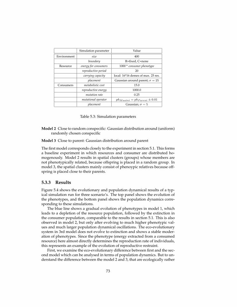
Simulation parameter Value

Environment size 400

boundary R=fixed, C=none

Resource energy for consumers 1000 * consumer phenotypereproductive period 20

carrying capacity local: 16*16 demes of max. 25 res.

placement Gaussian around parent; σ = 25

Consumers metabolistic cost 15.0

reproductive energy 1000.0

mutation rate 0.25

mutational operator phMuatnt = phParent ± 0.01

placement Gaussian; σ = 5

Table 5.3: Simulation parameters

Model 2 Close to random conspecific: Gaussian distribution around (uniform)randomly chosen conspecific

Model 3 Close to parent: Gaussian distribution around parent

The first model corresponds closely to the experiment in section 5.1. This formsa baseline experiment in which resources and consumer are distributed ho-mogenously. Model 2 results in spatial clusters (groups) whose members arenot phenotypically related, because offspring is placed in a random group. Inmodel 3, the spatial clusters mainly consist of phenoypic relatives because off-spring is placed close to their parents.

5.3.3 Results

Figure 5.4 shows the evolutionary and population dynamical results of a typ-ical simulation run for three scenario’s. The top panel shows the evolution ofthe phenotypes, and the bottom panel shows the population dynamics corre-sponding to these simulations.

The blue line shows a gradual evolution of phenotypes in model 1, whichleads to a depletion of the resource population, followed by the extinction inthe consumer population, comparable to the results in section 5.1. This is alsoobserved in model 2, but only after evolving to much higher phenotypic val-ues and much larger population dynamical oscillations. The eco-evolutionarysystem in 3rd model does not evolve to extinction and shows a stable moder-ation of phenotypes. Since the phenotype (energy extracted from a consumedresource) here almost directly determines the reproduction rate of individuals,this represents an example of the evolution of reproductive restraint.

First, we examine the eco-evolutionary difference between first and the sec-ond model which can be analysed in terms of population dynamics. But to un-derstand the difference between the model 2 and 3, that are ecologically rather

73

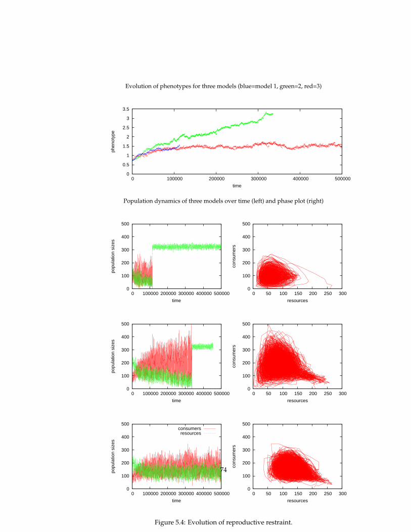
Evolution of phenotypes for three models (blue=model 1, green=2, red=3)

0

0.5

1

1.5

2

2.5

3

3.5

0 100000 200000 300000 400000 500000

phen

otyp

e

time

Population dynamics of three models over time (left) and phase plot (right)

0

100

200

300

400

500

0 100000 200000 300000 400000 500000

popu

latio

n si

zes

time

0

100

200

300

400

500

0 50 100 150 200 250 300

cons

umer

s

resources

0

100

200

300

400

500

0 100000 200000 300000 400000 500000

popu

latio

n si

zes

time

0

100

200

300

400

500

0 50 100 150 200 250 300

cons

umer

s

resources

0

100

200

300

400

500

0 100000 200000 300000 400000 500000

popu

latio

n si

zes

time

consumersresources

0

100

200

300

400

500

0 50 100 150 200 250 300

cons

umer

s

resources

Figure 5.4: Evolution of reproductive restraint.

74

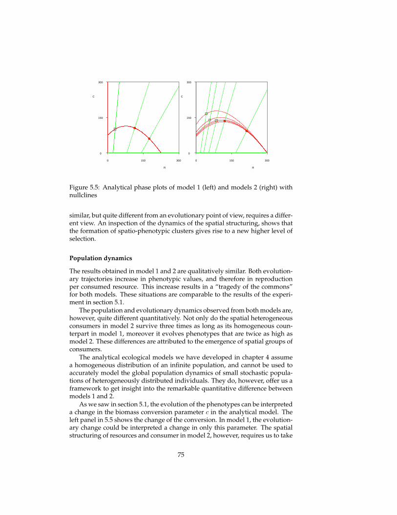
150

0

C

3001500

R

300

150

0

C

3001500

R

300

Figure 5.5: Analytical phase plots of model 1 (left) and models 2 (right) withnullclines

similar, but quite different from an evolutionary point of view, requires a differ-ent view. An inspection of the dynamics of the spatial structuring, shows thatthe formation of spatio-phenotypic clusters gives rise to a new higher level ofselection.

Population dynamics

The results obtained in model 1 and 2 are qualitatively similar. Both evolution-ary trajectories increase in phenotypic values, and therefore in reproductionper consumed resource. This increase results in a “tragedy of the commons”for both models. These situations are comparable to the results of the experi-ment in section 5.1.

The population and evolutionary dynamics observed from both models are,however, quite different quantitatively. Not only do the spatial heterogeneousconsumers in model 2 survive three times as long as its homogeneous coun-terpart in model 1, moreover it evolves phenotypes that are twice as high asmodel 2. These differences are attributed to the emergence of spatial groups ofconsumers.

The analytical ecological models we have developed in chapter 4 assumea homogeneous distribution of an infinite population, and cannot be used toaccurately model the global population dynamics of small stochastic popula-tions of heterogeneously distributed individuals. They do, however, offer us aframework to get insight into the remarkable quantitative difference betweenmodels 1 and 2.

As we saw in section 5.1, the evolution of the phenotypes can be interpreteda change in the biomass conversion parameter c in the analytical model. Theleft panel in 5.5 shows the change of the conversion. In model 1, the evolution-ary change could be interpreted a change in only this parameter. The spatialstructuring of resources and consumer in model 2, however, requires us to take

75

several other parameters in the analytical model into account next to the con-version parameter c.

The heterogenous spatial distribution of resources in model 2 causes theglobal carrying capacity K to be variable. The phase plots in figure 5.4 showsthat the global carrying capacity realised in model 1, with approximate homo-geneous consumer distribution, is lower than the others. This can be under-stood from the local growth of resources and consumers. Random placementof consumers in locations prevents the formation of resource clusters, becausethe resources are consumed before a cluster can be grown. When consumersare in groups, however, resources are depleted in some areas, but can flourishand form clusters where consumers are scarce. Therefore, the global carryingcapacity is larger in the heterogenous model 2 than in homogeneous model 1(see fig. 5.5).

Another implication of the formation of consumer groups, is the increaseof consumer interference e between consumers. The consumers in model 2 areexpected to experience more interference from their neighbours. Moreover, thelevel of interference is indirectly related to the phenotype, since higher pheno-types causes more dense groups, in which the consumer interference increaseseven more. Since higher consumer interference e results increased ecologicalstability, the evolution towards instability (by increase of the conversion pa-rameter c) is slightly inhibited by increased interference in situations with spa-tial heterogeneity (see fig. 5.5).

Although in both models, evolution causes an increase of the biomass con-version parameter c, the quantitative differences between model 1 and model2 can be understood in terms of an increased global carrying capacity K dueto resource heterogeneity, and increased consumer interference e due to con-sumers heterogeneity.

Groups

The evolutionary difference between model 2 and 3 as shown in the top panelin figure 5.4 cannot be attributed to such differences in population dynam-ics. In both experiments, offspring are placed close to other consumers whichgives rise to (moving and viscous) groups of consumer individuals with thesimilar ecological consequences. To understand why evolutionary dynamicsin one case leads to extinction while the other shows moderation and survival,a closer look at the group dynamics is required.

The consumer population organises itself into spatial clusters of consumerindividuals, that we call groups. Groups are formed by reproduction of in-dividuals, but persist over many generations of its members. Groups movearound, divide and interact with each other, break down due to dispersion orgo extinct. In a sense, they have a life cycle of their own.

The top panel of fig. 5.6 shows snapshots of the spatial distribution of theconsumers population over the environment, with the colour representing thephenotypes relative to the others. In scenario 2 (left panel), the groups are

76

phenotypically mixed, while the individuals in the groups in scenario 3 (rightpanel) shows strong phenotypic similarity.

The short term spacetime plots in fig. 5.6 illustrates the movement of con-sumer groups over time. The spacetime plots presented here are created byrecording the x-positions of consumers that inhabit a slice of the snapshot (with25 < y < 75) at a fixed interval.

Within-group selection

The difference between the two short term plots (taken over period 200000-210000) lies mainly in the phenotypic distribution. The groups in model 2 arephenotypically mixed. This is most clear in the leftmost region of the plot formodel 2 in which groups are observed that contain red and blue phenotypes.These are, in fact, individuals of two distinct (quasi)species that have emergedjust before (the only speciation event observed in model 2, see top panel infig. 5.4). Since the individuals of these phenotypically distinct species com-pete with other directly within spatial groups, the blue (lower) phenotypes arequickly outcompeted by the red (higher) phenotypes, because the latter repro-duce faster. The phenotypic differences within groups in the rest of the plotis smaller, i.e. there are no distinct species, because phenotypic variation issuppressed due to global mixing of phenotypes.

Differential reproduction in individual selection acts best if all individu-als/phenotypes interact with each other, and are evaluated relative to all oth-ers in a well-mixed situation. Since individuals interact locally with others intheir neighbourhood, the phenotypical composition of this neighbourhood in-fluences the selective pressure. When the spatial distribution of phenotypesbecomes structured into groups, individuals mostly interact with individualsthat are phenotypic relatives, and therefore distinct phenotypes are sparselyevaluated against each other.

The short term spacetime plot for model 3 in fig. 5.6 shows groups withindividuals that are phenotypically similar. Individuals in these groups mostlycompete with similar individuals. Because the within-group variation is low,individual selection has little substrate and operates relatively slowly.

Because the individuals that make up a group interact and reproduce lo-cally, phenotypes are not frequently evaluated against individuals of othergroups. Therefore, a group with relatively low phenotypes is able to maintainitself, even when groups with much faster reproducing individuals are alreadypresent in the environment.

If individual selection pressures differ between homogeneous (model 1 and2) and heterogeneous (model 3) spatial distribution of phenotypes, this is ex-pected to be reflected in the observed population-level variation. Figure 5.7shows the standard deviation of the phenotypes present in the population overevolutionary time for the three models (moving average of 1000 timesteps).Sudden increases in variation in model 2 and 3 indicate speciation events. Thephenotypic variation in model 3 is indeed significantly higher than the othermodels over the entire course of evolution.

77

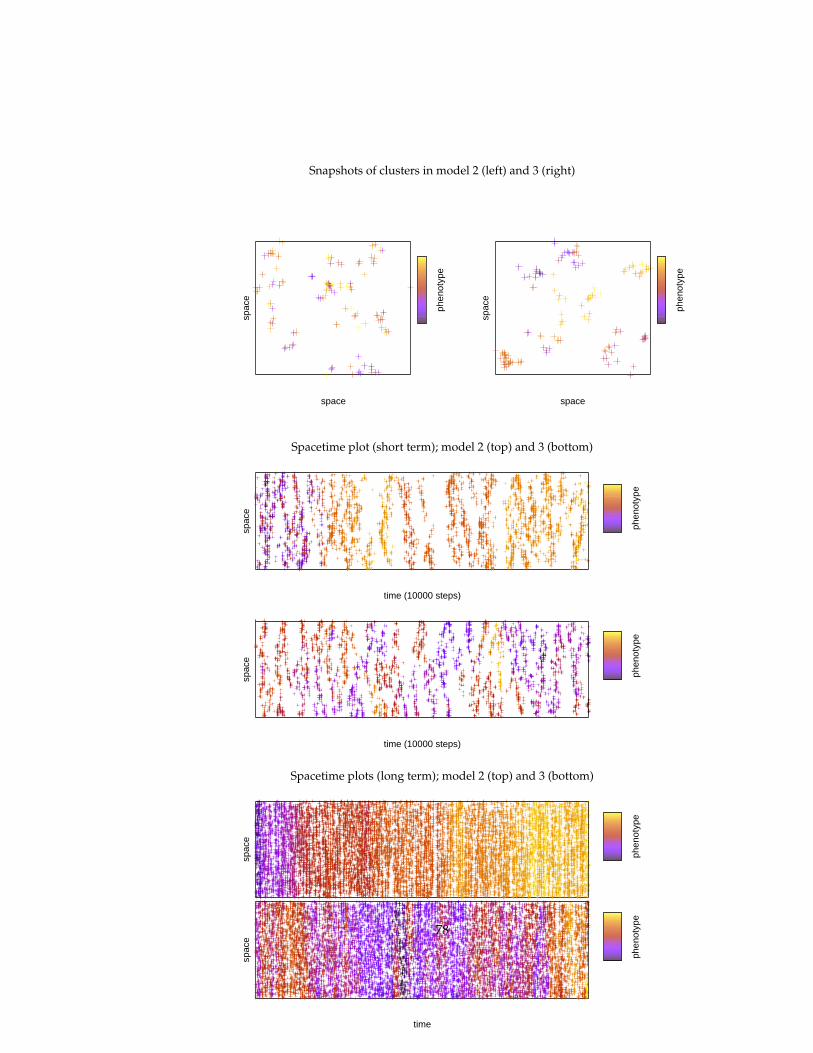
Snapshots of clusters in model 2 (left) and 3 (right)

phen

otyp

e

space

spac

e

phen

otyp

e

space

spac

e

Spacetime plot (short term); model 2 (top) and 3 (bottom)

phen

otyp

e

time (10000 steps)

spac

e

phen

otyp

e

time (10000 steps)

spac

e

Spacetime plots (long term); model 2 (top) and 3 (bottom)

phen

otyp

e

time

spac

e

phen

otyp

e

spac

e

Figure 5.6: Spatial self-clustering and evolution.

78

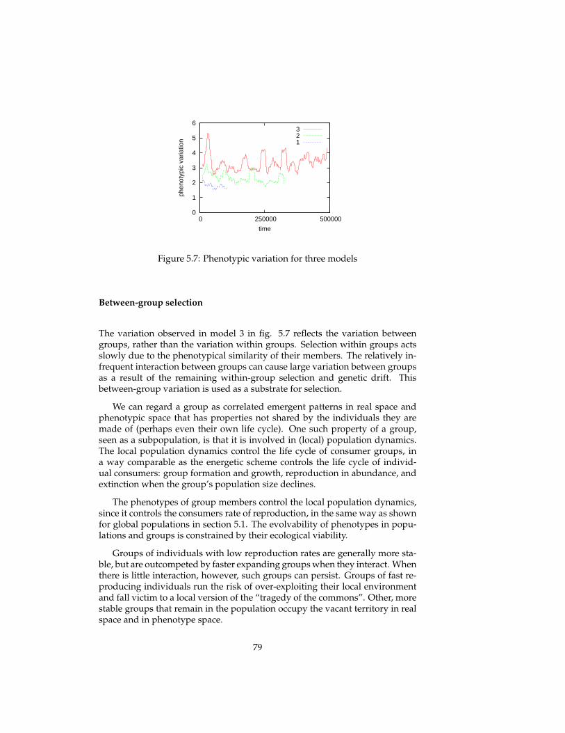
0

1

2

3

4

5

6

0 250000 500000

phen

otyp

ic v

aria

tion

time

321

Figure 5.7: Phenotypic variation for three models

Between-group selection

The variation observed in model 3 in fig. 5.7 reflects the variation betweengroups, rather than the variation within groups. Selection within groups actsslowly due to the phenotypical similarity of their members. The relatively in-frequent interaction between groups can cause large variation between groupsas a result of the remaining within-group selection and genetic drift. Thisbetween-group variation is used as a substrate for selection.

We can regard a group as correlated emergent patterns in real space andphenotypic space that has properties not shared by the individuals they aremade of (perhaps even their own life cycle). One such property of a group,seen as a subpopulation, is that it is involved in (local) population dynamics.The local population dynamics control the life cycle of consumer groups, ina way comparable as the energetic scheme controls the life cycle of individ-ual consumers: group formation and growth, reproduction in abundance, andextinction when the group’s population size declines.

The phenotypes of group members control the local population dynamics,since it controls the consumers rate of reproduction, in the same way as shownfor global populations in section 5.1. The evolvability of phenotypes in popu-lations and groups is constrained by their ecological viability.

Groups of individuals with low reproduction rates are generally more sta-ble, but are outcompeted by faster expanding groups when they interact. Whenthere is little interaction, however, such groups can persist. Groups of fast re-producing individuals run the risk of over-exploiting their local environmentand fall victim to a local version of the “tragedy of the commons”. Other, morestable groups that remain in the population occupy the vacant territory in realspace and in phenotype space.

79

Individual and group selection

Group selection in model 3 uses the variation between the local population dy-namical properties of spatial self-structured groups as a substrate. It acts bytruncating the evolution of phenotypes through local “tragedies of the com-mons”. The direction of the group selection pressure is opposite to the di-rection of individual selection. While individual selection favours “selfish”consumers, group selection favours “altruistic” consumer that restrain theirreproduction.

5.3.4 Conclusion

In this experiment, the impact of spatial self-structuring on ecological and evo-lutionary dynamics on a resource-consumer system was studied.The formation of spatial groups of resources and consumers, as a result of localdefinition of carrying capacity and placement of offspring, causes improvedecological stability. This ecological difference between spatial homogeneousand heterogeneous distribution of resources and consumers (i.e. model 1 and2) was understood in terms of the analytical model as an increased global car-rying capacity of resources, and increased consumer interference in consumergroups. The evolutionary dynamics in both models is qualitatively similar inthat they eventually result in the extinction of the consumer population. Evo-lution in the spatially heterogeneous ecosystem however differs quantitativelyfrom the homogeneous system as it results in the evolution of much higherrates of reproduction in the consumer population before going extinct. Thisevolutionary difference is due to the increased ecological stability in spatiallyheterogeneous systems, which causes high reproductive rates to be ecologi-cally viable and thus put a weaker constraint on the evolutionary dynamics.

Although consumer individuals in model 2 are spatially clustered, theirphenotypes are distributed over these clusters. In model 3, consumers andtheir phenotypes are self-structued in groups. A comparison between the re-sults of these two models show that spatial self-structuring has a major impacton the outcome of the selection process.

Since the phenotypic variation in groups in model 2 is greater than in model3, individual selection operates more effectively in the former. Since thereis little within-group variation in model 3, selection on the basis of individ-ual differences in reproduction has little substrate. The remaining individualselection pressures and random genetic drift causes the between-group vari-ation to grow. Initially, faster growing groups outcompete slower growinggroups. Above a critical phenotypic level, groups that over-exploit their lo-cal environment become involved in a local “tragedy of the commons”. Thebetween-group variation ensures that more stable groups exist that occupy thevacancy in real space and phenotype space, once the resource population hasgrown back. At a population level, this results on the evolution of reproduc-tive restraint. Since restraining reproduction does not increase the number of

80

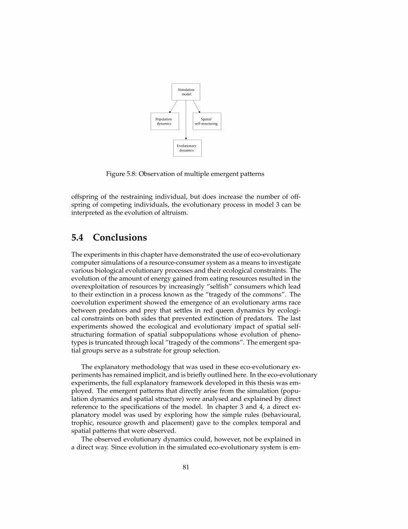
Simulation model

Population dynamics

Spatialself-structuring

Evolutionarydynamics

Figure 5.8: Observation of multiple emergent patterns

offspring of the restraining individual, but does increase the number of off-spring of competing individuals, the evolutionary process in model 3 can beinterpreted as the evolution of altruism.

5.4 Conclusions

The experiments in this chapter have demonstrated the use of eco-evolutionarycomputer simulations of a resource-consumer system as a means to investigatevarious biological evolutionary processes and their ecological constraints. Theevolution of the amount of energy gained from eating resources resulted in theoverexploitation of resources by increasingly “selfish” consumers which leadto their extinction in a process known as the “tragedy of the commons”. Thecoevolution experiment showed the emergence of an evolutionary arms racebetween predators and prey that settles in red queen dynamics by ecologi-cal constraints on both sides that prevented extinction of predators. The lastexperiments showed the ecological and evolutionary impact of spatial self-structuring formation of spatial subpopulations whose evolution of pheno-types is truncated through local “tragedy of the commons”. The emergent spa-tial groups serve as a substrate for group selection.

The explanatory methodology that was used in these eco-evolutionary ex-periments has remained implicit, and is briefly outlined here. In the eco-evolutionaryexperiments, the full explanatory framework developed in this thesis was em-ployed. The emergent patterns that directly arise from the simulation (popu-lation dynamics and spatial structure) were analysed and explained by directreference to the specifications of the model. In chapter 3 and 4, a direct ex-planatory model was used by exploring how the simple rules (behavioural,trophic, resource growth and placement) gave to the complex temporal andspatial patterns that were observed.

The observed evolutionary dynamics could, however, not be explained ina direct way. Since evolution in the simulated eco-evolutionary system is em-

81

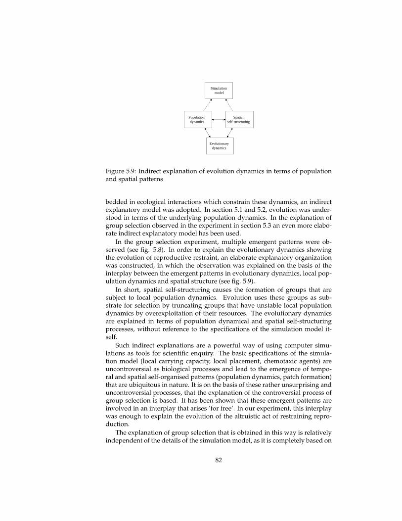
Simulation model

Population dynamics

Spatialself-structuring

Evolutionarydynamics

Figure 5.9: Indirect explanation of evolution dynamics in terms of populationand spatial patterns

bedded in ecological interactions which constrain these dynamics, an indirectexplanatory model was adopted. In section 5.1 and 5.2, evolution was under-stood in terms of the underlying population dynamics. In the explanation ofgroup selection observed in the experiment in section 5.3 an even more elabo-rate indirect explanatory model has been used.

In the group selection experiment, multiple emergent patterns were ob-served (see fig. 5.8). In order to explain the evolutionary dynamics showingthe evolution of reproductive restraint, an elaborate explanatory organizationwas constructed, in which the observation was explained on the basis of theinterplay between the emergent patterns in evolutionary dynamics, local pop-ulation dynamics and spatial structure (see fig. 5.9).

In short, spatial self-structuring causes the formation of groups that aresubject to local population dynamics. Evolution uses these groups as sub-strate for selection by truncating groups that have unstable local populationdynamics by overexploitation of their resources. The evolutionary dynamicsare explained in terms of population dynamical and spatial self-structuringprocesses, without reference to the specifications of the simulation model it-self.

Such indirect explanations are a powerful way of using computer simu-lations as tools for scientific enquiry. The basic specifications of the simula-tion model (local carrying capacity, local placement, chemotaxic agents) areuncontroversial as biological processes and lead to the emergence of tempo-ral and spatial self-organised patterns (population dynamics, patch formation)that are ubiquitous in nature. It is on the basis of these rather unsurprising anduncontroversial processes, that the explanation of the controversial process ofgroup selection is based. It has been shown that these emergent patterns areinvolved in an interplay that arises ’for free’. In our experiment, this interplaywas enough to explain the evolution of the altruistic act of restraining repro-duction.

The explanation of group selection that is obtained in this way is relativelyindependent of the details of the simulation model, as it is completely based on

82

generic biological self-organised processes (albeit emerging from a simulationmodel). Therefore, such explanations are much less sensitive to the criticismthat the outcome of the simulations is the product of the (often opaque) spe-cific implementation of the simulation. Having overcome this major criticismtowards artificial life models by indirect explanation, the use of complex simu-lation models as scienfitic tools for theoretical biological has become plausible.

83

Chapter 6

Conclusions

In this thesis, a versatile spatially explicit individual-based simulation modelwas presented that facilitates the study of the combination of situated interac-tion, self-organised collective behaviours and evolution by natural selection. Itprovides a platform for investigation of the interplay of processes at differentlevels of organization: behavioural interactions between individuals, spatialand temporal patterns on an ecological scale, and evolutionary dynamics of(co)evolving populations. The simulation model facilitates the construction ofmodels that share the focus on individual embodiment and situatedness as inautonomous robotics, as well as the collective and evolutionary approaches inartificial life. The combination of the development of the virtual life simula-tion model, with providing it with a sound embedding in theoretical ecologyand the use of direct and indirect explanations, constitute an important steptowards closing the gap between models used in embodied cognitive scienceand theoretical biology.

This concluding chapter provides a brief discussion of the results of simu-lation experiments in terms of the main background concepts as presented inchapter 2 (section 6.1). For more elaborate conclusions about specific ecologi-cal and eco-evolutionary simulations, the reader is referred to the conclusiongiven above. After the summary, we proceed to draw general conclusions withrespect to the methodological issues raised in section 1.3 about the scientific useof complex simulations (section 6.2).

6.1 Summary

We have seen that the virtual life simulation model incorporates the variousconcepts and themes that were examined in chapter 2.

84

Situated interaction

The simulated individuals can be simple static plant-like individuals, or mobilesituated agents equipped with sensors, effectors, and a (neural) control system.The consumer individuals that are used in the experiments in this thesis, imple-ment a simple control architecture similar to the Braitenberg vehicle (type 2b,see fig. 2.2). When these situated agents inhabit the same environment, andalter aspects of this environment, the behaviour of one individual influencesthe behaviour of others by a process of stigmergy from which spatiotemporalpatterns can arise.

Self-organization

In the ecological simulations in chapters 3 and 4, the stigmergic and trophic in-teractions gave rise to self-organised temporal patterns in population dynam-ics and spatial self-structuring. The emergent patterns in population dynamicsthat were observed in simulations show that local interactions between simpleindividuals agents results in the formation of global patterns. This enabled usto capture the global dynamics in terms of an analytical model, which allowedus to predict and control emergent dynamics of the simulated ecosystem.

Evolution

By including variation in the population along inheritable and mutable traits,the experiments in chapter 5 have shown that eco-evolutionary simulationsgive rise to interesting patterns in population dynamics, spatial self-structuringand evolutionary dynamics. Evolution is not modelled as an optimization pro-cess (as in traditional genetic algorithms), but as a process of adaptation inwhich an evolving population adapts to the ecological challenges of survivaland reproduction. This was sufficient to model natural selection of “selfish”consumer leading to a “tragedy of the commons”, evolutionary arms racesand red queen effect in a coevolutionary setting, and group selection as re-sulting from the interplay between local population dynamics and spatial self-structuring.

It seems reasonable to conclude that the aims of the virtual life model, as statedin the introduction, has been satisfied. The virtual life model has been shownto be capable of simulating situated interaction, self-organized collective be-haviour and evolution by natural selection. Moreover, the model has provenuseful in the effort of the study of the interplay between emergent patterns thatarise from the above mentioned processes.

85

6.2 Discussion

Theoretical embedding

The ability to construct complex simulation models does not, by itself, rendersuch simulation useful as tools for scientific enquiry, however. To be able tointerpret simulation results and use them in the scientific theory construction,the model needs to be embedded in, or related to, a well-understood theoreticalframework. This is, of course, true for all simulation models, but is especiallyimportant for complex simulations such as the virtual life model, as been illus-trated by the lack of such theoretical embedding of the PolyWorld simulator.

In the construction of the virtual life model, the theoretical embedding andtractability have been an integral part of the development. The theoreticalframework has been provided by the well-studied models of theoretical ecol-ogy, as laid down in chapter 4. This has provided a useful framework fromwhich simulations can be controlled and to which results can be compared andunderstood.

We have use these ecological models in a slightly odd way. The simula-tion model was used as a model for ecosystems, and the ODE models wereused as analytical model for the simulation model. The latter is a more power-ful formalism to study the interplay between generic biological processes thanthese classic state-variables models in many respects, due to its spatial andindividual-based nature. It is more powerful in the sense that it allows thestudy of the interplay between many processes that have traditionally beenstudied separately and has previously been unavailable. Despite this fact, thesimulation experiments and their analysis in this thesis has shown that the clas-sical analytical models has not lost their value. They have served here to un-derstand the emergent population dynamics in terms of density dependences,to control the population dynamics in the simulated ecosystems, and to un-derstand evolutionary dynamics in terms of population dynamics. Moreover,analytical models have guided the design of the simulation model and the var-ious experiments themselves. Most simulation experiments presented in thisthesis replicated the results of existing theoretical work using (more) formalmodels (enrichment, tritrophic foodchain, evolution, coevolution, group selec-tion), and is therefore itself part of this modelling approach.

But perhaps the most important way in which these theoretical model havebeen proven useful in analyzing simulation results is their use as baseline mod-els to which the results of relaxing of their implicit assumptions (infinite popu-lation sizes, monomorphic and well-mixed populations) can be compared andunderstood. In a sense, simulation results only tend to get interesting wherethe applicability of ODE models breaks down and the simulation show qual-itatively different behaviour. There is no way of telling what is interesting,however, without knowing what is not.

86

Indirect explanation

In chapter 1, we have identified the direct and indirect explanatory strategiesas two ways to use artificial life models and interpret their results. Both havebeen applied in this thesis, but the focus was on the indirect way of interpretingthe simulation results.

An example of direct explanation was provided for the regular patterns inthe population dynamics that were observed in the simulations. These wereinterpreted as an emergent property of the stigmergic and trophic interactionsbetween static resource and chemotaxic consumer individuals. This statementrelates the observed phenomenon directly to the specifications of the simula-tion model1. This can be interesting from the point of view of behaviouralecology, since it enables the study of the relation between situated behaviourand the ecological processes it gives rise to. It is not unexpected, however, sinceit merely restates that simple local interactions can give rise to complex globalpatterns.

We have also seen that when phenotypic variation and spatial heterogene-ity are allowed in the simulation model, the system gives rise to multiple emer-gent patterns: in population dynamics, in phenotype space, and in spatial dis-tribution. In these cases, an explanation that directly relates the observed phe-nomenon to specifications of the model is often not sufficient, and sometimesnot even necessary. The evolutionary arms race and red queen dynamics wererelated to population dynamics, and the evolution of reproductive restraintwas related to spatial distribution. Here, the emergent patterns in evolution-ary dynamics are understood in term of patterns that are themselves emergentproperties of the simulation model. Instead of focusing on the self-organizingprocesses themselves, we have studied the interplay between them, and usedthis as an explanatory model.

This strategy potentially renders theory formation based on simulation re-sults more generic. Indirect explanantions are based on an organizational struc-ture between emergent higher level patterns and is therefore less dependent onthe implementation details of the model. Explanations of processes obtainedin this way are relatively independent of the details of the simulation model, asthey are based on generic biological self-organised processes. Therefore, suchexplanations are much less sensitive to the criticism that the outcome of thesimulations is the product of the (often opaque) specific implementation of thesimulation. Indirect explanatory models enable the use of artificial life simu-lations as scientific tools in a fashion that trancends the ’simple to complex’paradigm by allowing the study of the ’complex to complex’.

The latter is essential in biological science to be able to gain insight in theinterplay between processes at the different level of organization in biologicalsystems (e.g. molecules, cells, organisms, ecosystems), and to explain the exis-

1If one considers the stigmergic interactions itself as an emergent property of the spatial andchemotaxic behaviour of consumers, one could be argue that this is indirect explanation as well.Here, stigmergy is assumed to be the self-organizing process itself, instead of the property thisprocess gives rise to.

87

tence of these multiple levels in the first place (e.g. the origin of life). We believethat it is essential for (embodied) cognitive science as well, since it studies a dif-ferent part of the same multi-level spectrum, and also attempts to explain theemergence of major transitions (e.g. origin of sociality and cognition). There-fore, we feel that complex artificial life simulation, combined with a theoreticalbiological embedding and an indirect explanatory framework, is a new andvaluable tool for cognitive science.

88

Bibliography

A. Adamatzky and M. Komosinski. Artificial life models in software. Springer,2005.

R. Axelrod and W. Hamilton. The evolution of cooperation. Science, 211(4489):1390–1396, 1981.

J.R. Beddington. Mutual interference between parasites or predators and itseffect on searching efficiency. Journal of Animal Ecology, 44:331–340, 1975.

M.C. Boerlijst and P. Hogeweg. Self-structuring and selection: spiral waves as asubstrate for evolution. In Langton, Taylor, Farmer, and Rasmussen, editors,Artificial Life II, pages 255–276. Addison-Wesley, 1991.

E. Bonabeau, M. Dorigo, and G. Theraulaz. Swarm intelligence: from natural toartificial systems. Oxford University Press, 1999.

V. Braitenberg. Vehicles: experiments in synthetic psychology. MIT Press, 1984.

R. Brooks. Achieving artificial intelligence through building robots. MIT Tech-nical report, 1985.

S. Camazine, J. Deneubourg, N. Franks, J. Sneyd, G. Theraulaz, andE. Bonabeau. Self-organization in biological systems. Princeton UniversityPress, 2001.

L. Carroll. Through the looking glass. Mansfield and Wessels, New York, 1899.

A. Channon. Towards the evolutionary emergence of increasngly complex ad-vantageous behaviours. International Journal of Systems Science, Special Issue,2000.

W. Clancey. The frame of reference problem in the design of intelligent ma-chines. In K. van Lehn, editor, Architecture for Intelligence, pages 357–424,1991.

I. Couzin and J. Krause. Self-organization and collective behavior in verte-brates. Advances in the Stdu of Behavior, 32:1–75, 2003.

89

C. Darwin. On the origins of species by means of natural selection, or the preservationof favoured species in the struggle for life. J. Murray London, 1859.

R. Dawkins. The selfish gene. Oxford University Press, 1976.

R. Dawkins and D. Krebs. Arms races between and within species. Proceedingsof the Royal Society of London, 205:489–511, 1979.

R. de Boer. Modelling population dynamics: a graphical approach. Lecturenotes, Theoretical Biology/Bioinformatics group, Utrecht University., 2006.

D.L. DeAngelis, R.A. Goldstein, and R.V. O’Neill. A model for trophic interac-tions. Ecology, 56:881–892, 1975.

J. Deneubourg, J. Pasteels, and J. Verhaege. Probabilistic behaviour in ants: astrategy of errors? Journal of Theoretical Biology, (105):259–271, 1983.

E. di Paolo. On the evolutionary and behavioral dynamics of social coordination:models and theoretical aspects. PhD thesis, University of Sussex, 1999.

H. Dreyfus. A phenomenology of skill acquisition as a basis for a Merleau-Pontian non-representationalist cognitive science.

M. Eigen. Selforganization of Matter and the Evolution of Biological Macro-molecules. Naturwissenschaften, 58:465–523, 1971.

M. Eigen and P. Schuster. The Hypercycle: A Principle of Natural Self-Organization.Springer, Berlin, 1979.

S. Forrest and M. Mitchell. Genetic algorithms and artificial life. Artificial life, 1(3):267–289, 1994.

C. Gershenson and F. Heylighen. When can we call a system self-organizing?In W. et al Banzhaf, editor, ECAL-7, pages 606–614. Springer, 2003.

L.R. Ginzburg. Assuming reproduction to be a function of consumption raisesdoubts about some popular predator-prey models. Journal of Animal Ecology,67:325–327, 1998.

P. Grasse. La theorie de la stigmergie: essai d’interpretation du comportementdes termites constructeurs. Insectes Sociaux, 6:41–81, 1959.

V. Grimm. Ten years of individual-based modelling in ecology: what have welearned and what could we learn in the future? Ecological modelling, 115(2-3):129–148, 1999.

W. Hamilton. The genetical evolution of social behaviour (I and II). Journal ofTheoretical Biology, 7:1–16, 17–52, 1964.

G. Hardin. The Tragedy of the Commons. Science, 162(3859):1243–1248, 1968.

90

I. Harvey, D. Husbands, A. Thompson, and N. Jakobi. Evolutionary robotics:the Sussex approach. Robotics and Autonomous Systems, 20:205–224, 1997.

A. Hasting and T. Powell. Chaos in a three-species food chain. Ecology, 72:896–903, 1991.

F. Heylighen. The science of self-organization and adaptivity. The Encyclope-dia of Life Support Systems, 1999.

P. Hogeweg and B. Hesper. Individual-based modelling in ecology. Mathemat-ical and commputer modelling, 13(6):83–90, 1990.

C.S. Holling. Some charcteristics of simple types of predation and paratism.The Canadian Entomologist, 91:385–398, 1959.

C.S. Holling. Functional response of predators to prey density and its rolein mimicry and population regulation. Memoirs of Etnomological Society ofCanada, 45:3–60, 1965.

M. Hutson, D. DeAngelis, and W. Post. New computer models unify ecologicaltheory. BioScience, 1988.

A.R. Ives and V. Jansen. Complex dynamics in stochastic tritrophic models.Ecology, 79:1039–1052, 1998.

C. Johnson and M. Boerlijst. Selection at the level of the community: the im-portant of spatial structure. Trends in Ecology and Evolution, 17:83–90, 2002.

M. Komosinski. The Framsticks system: versatile simulator of 3D agents andtheir evolution. Kybernetes: International Journal of Systems & Cybernetics, 32(1/2):156–173, 2003.

M. Komosinski and A. Rotaru-Varga. From directed to open-ended evolutionin a complex simulation model. In Artificial Life VII, pages 293–299. MITPress, 2000.

M. Komosinski and S. Ulatowski. Framsticks: towards a simulation of a nature-like world, creature and evolution. In ECAL-5, pages 261–265, 1999.

A. Lotka. Elements of physical biology. Williams & Wilkins Co., Baltimore, 1925.

M. Maris and R. te Boekhorst. Exploiting physical constraints: heap formationthrough behavioural error in a group of robots. In IROS96, 1996.

J. Maynard-Smith and E. Szathmary. The major transitions in evolution. OxfordUniversity Press, 1995.

C. Melhuish and O. Holland. Stigmergy, self-organisation, and sorting in col-lective robotics. Artificial Life, 5(2):173–202, 1999.

F. Menczer and R. Belew. Latent energy environments. In Adaptive individualsin evolving populations: models and algorithms, pages 191–208, 1996.

91

M. Merleau-Ponty. Phenomenology of Perception. 1943. translation by ColinSmith 1963.

G. Miller. Artificial life as theoretical biology: How to do real science withcomputer simulations. In M. Boden, editor, Philosophy of Artificial Life. OxfordUniversity Press, 1996.

S. Nolfi and D. Floreano. Evolutionary robotics: the biology, intelligence and tech-nology of self-orgnizing machines. MIT Press, 2000.

R. Pfeifer and C. Scheier. Understanding Intelligence. MIT Press, 1999.

T. Ray. An approach to the synthesis of life. In C. et al Langton, editor, Artificiallife II, 1991.

C. Reynolds. Flocks, herds, and schools: a distrubuted behavioral model. Com-puter Graphics, 21(4):25–34, 1987.

O. Rössler. Adequate Locomotion Strategies for an Abstract Environment: ARelational Approach. In Physics and Mathematics of the Nervous System, pages399–418. Springer, 1974.

N. Savill and P. Hogeweg. Evolutionary stagnation due to pattern-pattern in-teractions in a co-evolutionary predator-prey model. Artificial Life, 3:81–100,1997.

H. Simon. The sciences of the artificial. MIT Press, 1969.

M. van Baalen and D.A. Rand. The unit of selection in viscous population andthe evolution of altruism. Journal of Theoretical Biology, 143:631–648, 1998.

J.D. van der Laan and P. Hogeweg. Predator-prey coevolution: interactionsacross different timescales. Proceedings of Royal Society London, 259:35–42,1995.

L. van Valen. A new evolutionary law. Evolutionary Theory, 1:1–30, 1973.

V. Volterra. Variazone e fluttuazione del numero d’individui in specie animaliconviventi. Memorie della R. Acc. Naz. dei Lincei, 2:30–111, 1926.

G.C. Williams. Adaptation and natural selection: a critique of some current evolu-tionary thought. Princeton University Press, 1966.

D.S. Wilson. A theory of group selection. PNAS, 72(1):143–146, 1975.

D.S. Wilson and E. Sober. Reintroducing group selection to the human behav-ioral sciences. Behavioral and Brain Sciences, 17(4):585–654, 1994.

V. Wynne-Edwards. Animal dispersion in relation to social behaviour. Oliver &Boyd: Edinburgh, 1962.

92

V. Wynne-Edwards. Intergroup selection in the evolutionof social systems. Na-ture, 200:623–629, 1963.

L. Yaeger. Computational genetics, physiology, metabolism, neural systems,learning, vision, and behavior or PolyWorld: life in a new context. In Artifi-cial life III, 1994.

93

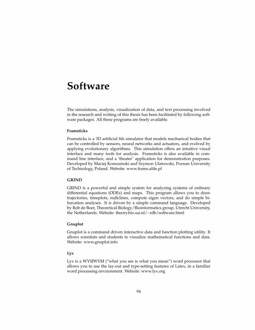
Software

The simulations, analysis, visualization of data, and text processing involvedin the research and writing of this thesis has been facilitated by following soft-ware packages. All these programs are freely available.

Framsticks

Framsticks is a 3D artificial life simulator that models mechanical bodies thatcan be controlled by sensors, neural networks and actuators, and evolved byapplying evolutionary algorithms. This simulation offers an intuitive visualinterface and many tools for analysis. Framsticks is also available in com-mand line interface, and a ’theater’ application for demonstration purposes.Developed by Maciej Komosinski and Szymon Ulatowski, Poznan Universityof Technology, Poland. Website: www.frams.alife.pl

GRIND

GRIND is a powerful and simple system for analyzing systems of ordinarydifferential equations (ODEs) and maps. This program allows you to drawtrajectories, timeplots, nullclines, compute eigen vectors, and do simple bi-furcation analyses. It is driven by a simple command language. Developedby Rob de Boer, Theoretical Biology/Bioinformatics group, Utrecht University,the Netherlands. Website: theory.bio.uu.nl/~rdb/software.html

Gnuplot

Gnuplot is a command driven interactive data and function plotting utility. Itallows scientists and students to visualize mathematical functions and data.Website: www.gnuplot.info

Lyx

Lyx is a WYSIWYM (“what you see is what you mean”) word processor thatallows you to use the lay-out and type-setting features of Latex, in a familiarword processing environment. Website: www.lyx.org

94