Viral system algorithm: foundations and comparison between

1

Viral System algorithm: foundations and comparison

between selective and massive infections

Pablo Cortés1*, José M. García1, Jesús Muñuzuri1, José Guadix1

1 Ingeniería Organización. Escuela Superior Ingenieros. University of Seville

c/ Camino de los Descubrimientos s/n.

E-41092. Seville – SPAIN

*corresponding author:

Email: [email protected]

Tel: +34 95 448 61 53

Fax: +34 95 448 72 48

Abstract.- This paper presents a guided and deep introduction to Viral Systems

(VS), a novel bio-inspired methodology based on a natural biological process

taking part when the organism has to give a response to an external infection.

VS has proven to be very efficient when dealing with problems of high

complexity. The paper discusses on the foundations of viral systems, presents

the main pseudocodes that need to be implemented and illustrates the

methodology application. A comparison between VS and other metaheuristics,

as well between different VS approaches is presented. Finally trends and new

research opportunities are presented for this bio-inspired methodology.

Keywords- Viral System, bio-inspired methodology, optimization, metaheuristic

1. Introduction

Viral Systems is a new bio-inspired methodology simulating the natural

biological process taking part when the organism has to give a response to an

2

external infection. Natural Immune System protects the organism from

dangerous extern agents such as viruses or bacteria. In this context, antibodies

try to protect the organism from such pathogens. Immune systems have a lot of

peculiarities that make them very attractive for computational optimization

(Cutello et al., 2007a and Cutello et al, 2007b). In certain manner, Viral System

(VS) makes use of the same infection-antigenic response concept from immune

systems, but from the perspective of the pathogen. That is, the virus infection

expansion corresponds to the feasibility region exploration, and the optimum

corresponds to the organism lowest fitness value.

Real optimization problems are complex, especially those that are classified as

NP-Hard. For such type of problems, available algorithms usually present

weaknesses and exact mathematical methods cannot guarantee the optimum of

the problem in a bounded time. So, several generalized metaheuristics (as

genetic algorithms, tabu search or simulated annealing among others) have

successfully tried to deal with such problems. Since the last decade, new

research is being undertaken in order to find other natural-life inspired methods

to solve this kind of problems. Examples of that are artificial life algorithms, in

particular predator prey type models, which are relatively closed to our VS. Van

Dyke Parunak (1997) presents a detailed description of such models in a multi-

agent system context.

The concept of viruses’ analogies has been mainly used as part of genetic

algorithms. For instance, Kubota et al. (1996) propose them as part of a specific

operator in genetic algorithms, and Saito (2003) has described the use of

genetic algorithms which make use of a virus evolutionary theory (GAV), and an

algorithm based on the conception of horizontal evolution caused by virus

3

infections. GAV is carried out by attacking a chromosome by a number of

viruses, and having the genes of the chromosome recombined by the attack.

The infection is allowed when the evaluation value goes up, but it falls into local

minima easily. In order to escape from these local minima, an infection which

makes the evaluation value worse in a small rate under small probability is

allowed as well. All these approaches do not fit with our definition of Viral

System as a new metaheuristic what we detail in this paper.

By now, applications of VS application has mainly tested in network problems

(Cortés et al, 2008 and Cortés et al, 2010). However, its application to other

context can be easily moved as this paper stands.

The rest of the paper follows with the presentation of the foundations of Viral

Systems in section two. Next, section three details the pseudocode for the two

types of considered infections. Section four includes a brief comparison

between the detailed two types of infection being presented in this paper. The

comparison is made for a well-known network flows problem. The fifth section

presents a problem example and illustrates the solution procedure using VS

methodology. The final section presents several conclusions and further

research opportunities.

2. Foundations of Viral Systems

2.1. Viruses, viral infections and organism antigenic response

Viruses are intracellular parasites shaped by nucleic acids, such as DNA or

RNA, and proteins. The protein generates a capsule, called a capsid, where the

4

nucleic acid is located. The capsid plus the nucleic acid shape the nucleus-

capsid, defining the virus. There is a high number of different types of viruses,

each of them showing a different and autonomous behaviour. However, the

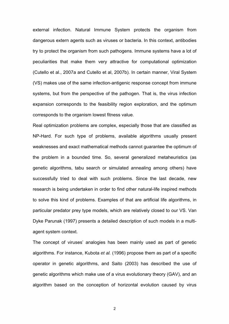
simplest and most common type of virus is the phage, a type of virus infecting

bacteria. Figure 1 depicts a traditional representation for such structure.

ξ Head

DNA (inside)Tail

Baseplate

Tail fiberξξ Head

DNA (inside)Tail

Baseplate

Tail fiber

Coliphagestructure

Figure 1 Coliphage structure

One of the main characteristics of viruses is the replication mechanism. The

phage (a common type of virus) does follow lytic replication process. Left side of

Figure 2 depicts the biological evolution of the virus infection following the next

steps:

1. The virus is adhered to the border of the bacterium. After that, the virus

penetrates the border being injected inside this one, (1) and (2) in Figure 2.

2. The infected cell stops the production of its proteins, beginning to produce

the phage proteins. So, it starts to replicate copies of the virus nucleus-capsids,

(3a) in Figure 2.

3. After replicating a number of nucleus-capsids, the bacterium border is

broken, and new viruses are released, (4a), which can infect near cells, (1), in

Figure 2.

5

The life cycle of the virus can be developed in more than one step. Some

viruses are capable of lodging in cells giving rise to the lysogenic replication.

This case is shown in the right side of Figure 2. It follows:

1. The virus infects the host cell, being lodged in its genome, (3b) in Figure 2

where a pro-phage (mutation) can arise.

2. The virus remains hidden inside the cell during a while until it is activated by

any cause, for example ultraviolet irradiation or X-rays, (i) in Figure 2. During

such time the cell reproduces itself normally.

3. The replication of cells altered, with proteins from the virus, starts. So,

lysogenic replication produces the genome alteration of the cell leading to a

procedure similar to a mutation process.

Phage DNA enters lytic or lysogenic cycle

New DNA and phage proteins are synthesized producing new viruses

Border cell broken, new phages are released

Phage DNA

Phage is adhered to the guest cell infecting its DNA

Bacteria chromosome

LyticCycle

LysogenicCycle

Many cell divisions

Phage DNA is integrated in the bacteria chromosome by recombining, becoming a

pro-phage (mutation)

The bacteria reproduces itself normally

Occasionally, the pro-phage could be removed from the bacterial

chromosome by other recombination giving place to a lytic cycle

Pro-phage

Figure 2 Lytic (left) and lysogenic (right) replication of viruses

However, some viruses have the property of leading an antigenic response in

the infected organism. In these situations an immune response is originated

causing the creation of antibodies. This is the specific case of phages.

6

So VS follows an exploration process that combines lytic replication to search

the neighbourhood of the existing solutions (which is one of the main features of

Tabu Search) and a mutation process (which is a characteristic of Genetic

Algorithms).

2.2. Computational description of Viral Systems

VS is an iterative method that runs during a maximum number of iterations, or

until the optimum is reached in case of a known optimum.

VS defines the clinical picture of an infected population as the description of all

the cells infected by viruses. Computationally, it includes the encoding of the

solution that is being explored (the genome of the cell that is infected, in

biological terms) and the number of nucleus-capsids being replicated, NR, (for

lytic replications) or the number of hidden generations, IT, (for lysogenic

replications). Thus the state of each virus is given by the three-tuple “cell

genome-NR-IT”. All these three-tuples corresponding to the cells infected by

viruses define the clinical picture.

Every cell infected by a virus develops a lytic or a lysogenic replication

according to a probability plt (for lytic replication) or plg otherwise, where plt + plg

= 1.

In case of lysogenic replications, the activation of the mutation process takes

place after a limit of iterations has passed (LIT). The value of LIT depends on

the cell’s health conditions, so a healthy cell (high value of the objective function

being minimised, f(x)) will have a low infection probability, i.e. the value of LIT

will be higher. An unhealthy cell, on the contrary, will have a lower value of LIT.

7

In case of lytic replications, a number of virus replications (NR) is calculated for

each iteration as a function of a binomial variable, Z, adding its value to the

current NR in the clinical picture. Z is calculated using a Binomial distribution

given by the maximum level of nucleus-capsids replicated, LNR, and the single

probability of one replication, pr,: Z = Bin (LNR , pr). LNR represents the limit to

break the cell border and to release the lodged viruses. As in the lysogenic

cycle, the value of LNR is set depending on the value of the objective function

being minimised, f(x). Thus cells with higher f(x) have lower probability of

getting infected, and therefore the value of LNR will be higher.

Two infections process have been defined for VS: massive infections where a

devastating infection reaches a high number of cells, and selective infection

where a parsimonious infection following a like-elitist process takes place. An

example of the first case is the Ebola virus with a rapid and massive infection

that very often produces the death of the patient in a few days, and an example

of the second one is the HIV virus, which through a step-by-step evolution

destroys the immune system during a process that can take years.

2.2.1. Massive infection

Once a massive infection takes place and viruses are liberated inside the

organism, each liberated virus will have a probability, pi, of infecting other new

cells of the neighbourhood. If the neighbourhood cardinality of x is defined as

|V(x)|, the number of cells infected by the virus in the neighbourhood can be

calculated as a binomial distribution given by Y = Bin (|V(x)|, pi).

On the other hand, in order to defend itself from the growth of the viral infection,

the Organism (the set of cells) responds by releasing antigens. In the clinical

8

picture, each one of the infected cells generates antibodies according to a

Bernoulli probability distribution A(x) = Ber (pan), where pan is the unitary

probability of generating antibodies by the cell x in the clinical picture. Hence,

the total population of infected cells generating antibodies is characterized by a

Binomial distribution of parameters: the size of the clinical picture, n, and the

probability of generating antibodies, pan: A(population) = Bin (n, pan).

Also, the antigenic response for every cell in the neighbourhood of an active

virus is estimated as a Bernoulli probability distribution given by the probability

of generating antibodies, pan: A(x’) = Ber (pan) : x’∈V(x). Therefore, the total

number of cells with antibodies in the neighbourhood will follow a Binomial

probability distribution given by the total size of the neighbourhood for all the

active viruses, |V(x)|, and the probability of generating antibodies, pan: A = Bin

(|V(x)|, pan).

In this situation, a Markovian Process defines the evolution of the clinical picture

(Cortés et al. 2008). Let ),...,,( LNR10 ππππ = be the probability of a cell with 0, 1, …

, LNR nucleus-capsids replicated. Equations (1-3) are satisfied in steady state.

P·ππ = ( 1 )

LNR ..., ,2 ,11

1 1

00=∀

⎟⎟

⎠

⎞

⎜⎜

⎝

⎛⋅

−= ∑

−

=− jp

p k

j

kkjj ππ ( 2 )

1... LNR10 =+++ πππ ( 3 )

To ensure computational control of the infection evolution, we can give (4) as an

adequate value for pan.

9

( )( ) nxVpn

xVpnp

i

ian

+−⋅⋅⋅

−⋅⋅⋅>

1|)(|1|)(|

LNR

LNR

π

π ( 4 )

Where |)(| xV is the average neighbourhood size for a specific problem.

However, we do not use the same value of pan for all the cells. In fact, a higher

value of f(x) implies a healthy cell and therefore this cell will have a higher

probability of developing an antigenic response. On the contrary, a cell with a

low value of f(x) represents an unhealthy cell with a lower probability of

developing an antigenic response. Thus we define for each cell its specific

pan(x). To deal with it in computational terms, we use a hypergeometric function,

where the cell with an inverse objective function evaluation, ( )xf1 , in ranking

position-i, has a probability of generating antibodies, pan(x), that is given by q(1-

q)i, with q equal to the probability of generating antibodies for the worst

individual. Finally, a residual probability remains, which is added to the worst

individual.

Figure 3 describes the algorithmic process. The original state is depicted by the

clinical picture on the left-hand side. The viruses reaching the level of nucleus-

capsids (LNR) break the border and start infecting new cells in their

neighbourhoods. The response of the Organism is characterized by the

antigenic response, liberating space in the clinical picture, and by creating

antibodies in cells located in the virus neighbourhood. This situation leads to a

new clinical picture, depicted on the right-hand side of the figure, with new

infected cells lodging viruses.

10

Genome of cell 1 NR1






Genome of cell i NRi

Genome of cell n-1 NRn-1

Genome of cell n NRn

It1

It2

It3

It4

It5

It6

Iti

Itn-1

Itn










It1

It2

It3

It4

It5

It6

Iti

Itn-1

Itn

Vi(x)

V6(x)

V1(x)

NR1, NR6, NRi ≥ LNR

Lytic replication Neighbourhood










It1

It2

It3

It4

It5

It6

Iti

Itn-1

Itn

Organism antigenic response

VIRUS PROCESS

ORGANISM PROCESS

ξξ

ξξ

ξξ

ξξ

ξξ

ξξ

ξξ

ξξ

ξξ

ξξ

ξξ

ξξ

ξξ

ξξ

ξξ

ξξ

ξξ

ξξ

VirusCell with antibodiesCell without antibodies

NEW

Clinical picture (t)

Antigenic response in clinical picture (cells: 2, 4 ,n-1)

Genome of cell 1 0Genome of cell 2 0Genome of cell 3 NR3

Genome of cell 4 0Genome of cell 5 NR5

Genome of cell 6 0

Genome of cell i 0

Genome of cell n-1 0Genome of cell n NRn

00It3

0It5

0

0

0Itn

Genome of cell 1 0Genome of cell 2 0Genome of cell 3 NR3

Genome of cell 4 0Genome of cell 5 NR5

Genome of cell 6 0

Genome of cell i 0

Genome of cell n-1 0Genome of cell n NRn

00It3

0It5

0

0

0Itn

NEW

NEW

NEW

NEW

NEW

Z = Bin (LNR , pr) Y = Bin (|V(x)|, pi)

A = Bin (|V(x)|, pan)A(population) = Bin (n, pan)

Clinical picture (t+1)

Figure 3 Algorithmic for lytic replication case in massive infections

2.2.2. Selective infection

Once a selective infection takes place and viruses are liberated inside the

organism, the virus selects a cell with a low value of f(x) in the neighbourhood.

However, the virus will not be able to infect those cells that have developed

antigens.

Higher values of f(x) imply healthy cells and therefore cells that have a higher

probability of developing antigenic responses. On the contrary, cells with low

value of f(x) imply unhealthy cells with lower probability of developing antigenic

responses. This effect is represented by the previously introduced

hypergeometric function.

11

Then, if the probability of generating antibodies for the case of cell x is pan(x),

A(x) is defined as a Bernoulli random variable: A(x) = Ber (pan(x)).

If cell x generates antibodies, the cell is not infected and it is therefore not

included in the new clinical picture. For recording this clinical picture we use the

original cell (that was infected by the virus and that reached the LNR limit) and

we initiate a lysogenic cycle for that cell.

Figure 4 defines the algorithm evolution for the infection. The initial state is on

the left-hand side: the virus process starts with viruses breaking the border and

starting the infection of new cells in their neighbourhoods. Each virus selects

the most promising cell, which is the least healthy cell. The Organism process is

characterized by the probability of antigenic response in the least healthy cell.

Those cells developing antibodies are not infected. Finally, the interaction (right

hand side of the figure) defines the new clinical picture, with new infected cells

lodging viruses. The cells generating antibodies follow a new lysogenic

replication.

12










It1

It2

It3

It4

It5

It6

Iti

Itn-1

Itn

Vi(x)

V6(x)

V1(x)

NR1, NR6, NRi ≥ LNR

Output ejectors: lytic replication Input sensors: neighbourhood

INTERACTIONORGANISM PROCESS

ξξ

ξξ

ξξ

ξξ

ξξ

ξξ

ξξ

ξξ

ξξ

ξξ

ξξ

ξξ

ξξ

ξξ

ξξ

ξξ

ξξ

ξξ

Virus

NEW

{ }nixgx i ,,1 , 0)(:K =∀≤=

VIRUS PROCESS

Lowest healthy cell without antigenic response(infected cell)Lowest healthy cell with antigenic response(non-infected cell)

A(x) = Ber (pan(x)

NEW

Healthy cell (non-infected cell)










It1

It2

It3

It4

It5

It6

Iti

Itn-1

Itn

Initiation of lysogenic cycle

Figure 4 Algorithm for lytic replication case in selective infection

3. VS pseudocodes

3.1. VS selective infection pseudocode

Table 1 describes the main functions to be considered for a selective infection.

The general pseudocode functions and procedures need to be complemented

with each specific problem procedures. These are mainly the neighbourhood

characterization and the problem-oriented lysogenic replication.

13

Table 1 General pseudocode for VS selective infection

procedure Virus_System(Nmax, Clinical_Size, plt ,pi, pan, pr, LNR, LIT) CP = ∅ /* Clinical Picture /* Get Initial Clinical Picture for i = 1 to Clinical_Size /* Get randomly a feasible solution and assign randomly a replication type CP(i) = Get_Random_Feasible_Solution() CP(i).Replicat_Type = Get_Random_Replication _Type(plt)

next do iterations = iterations + 1 i = Select_Random_Solution(Clinical_Size) if CP(i).Replicat_Type = ‘Lytic’ Then Lytic_Replication(CP(i), plt, pi, pan, pr, LNR) else Lysogenic_Replication(CP(i) , plt)

loop until iterations= Nmax or Check_Gap(CP) = True end Virus_System ------------------------------------------------------------------------------ procedure Litic_Replication (CS, plt ,pi, pan, pr, LNR) CS = Current solution /* Get the number of replicated nucleus-capsids z = Get_Random_Binomial_Probability(LNR, pr) do i = i + 1 if z < Binomial(i) then P(c).NR = P(c).NR + 1

loop until i = LNR or z ≥ Binomial(i) /* Check infection if CS.NR > CS.LNR then

/* Get the list VS of neighbouring solutions of CS in descending order regarding solution health VAS = Get_ Arranged_Neighbourhood(Vs) /* Get the clinical picture CP in ascending order regarding solution health CPA = Get_ Arranged_Clinical_Picture(CP) i = 1 for each S’∈VAS

if i <= |CPA| then replace = false do a = Get_Random_Binomial_Probability(|Vs| , pan) b = Get_Random_Binomial_Probability (|Vs|, pi) if a > pan and b > pi then /* Replace CPA(i) with a new solution CS’

CPA(i) = CS’ CPA(i).Replicat_Type = Get_Random_Replicat_Type(plt) replace = true

i = i + 1 loop until replace = true or i > |CPA|

end-for end Litic_Replication ------------------------------------------------------------------------------procedure Lysogenic_replication(CS, plt) CS.IT = CS.IT + 1 if CS.IT > CS.LIT then

s = Get_Random_Gen () /* apply move of mutation on CS CS

NEW = Mutation(CS, s) CS

NEW.Replicat_Type = Get_Random_Replication_Type(plt) return CS

end Lysogenic_replication

14

3.2. VS massive infection pseudocode

The main difference between massive and selective infection processes is the

infection activity every time the algorithm makes iteration. In the selective

infection case, only a single cell is infected whereas in the massive one, all cells

are infected at each iteration. However, lytic and lysogenic replications are the

same for both processes. Therefore, the differences in the pseudocode of the

massive process respect to the selective process only appear in the main

procedure. Table 2 shows the general procedure for the massive infection

process; meanwhile lytic and lysogenic procedures remain as the same

procedures showed in Table 1.

Table 2 General pseudocode for VS massive infection

4. A brief comparison between VS massive and selective

infections

In order to illustrate the performance of VS massive and selective infections and

the degree of complementarily between them depending on the specific

characteristics of the problem, we bring here a well-known network problem (the

Procedure Virus_System(Nmax , clinical_size , plt , pi , pan , LNR , LIT) CP = ∅ {Clinical Picture} iterations = 0 Get_Initial_Clinical_Picture(CP , clinical_size , plt) Do iterations = iterations + 1 For c = 1 to clinical_size If Replicat_Type(CP(c)) = ‘Lytic’ Then Lytic_Replication (c , LNR)

Else Lysogenic_Replication(c)

End If Next

Loop Until iterations= Nmax or Check_Gap(CP) = True End Procedure

15

Steiner tree problem) that has been previously dealt with in our previous works

(Cortés et al. 2008; and Cortés et al. 2010).

To test the two approaches, we used the OR-Library that can be accessed in

the website http://people.brunel.ac.uk/~mastjjb/jeb/info.html (Beasley, 2010),

considering series SteinC, SteinD and SteinE. We divided the Steiner tree

problem into three groups: Group No.1 is a low terminal density group that

contains problems with less than 15% of terminal nodes; group No. 2

corresponds to medium terminal density and consists of problems with more

than 15% and less than 30% of terminal nodes; and group No. 3 features

problems with more than 30% of terminals.

Tables 3, 4 and 5 show the results for each VS approach depending on the

terminals’ structure.

Table 3 Comparison on VS massive and selective infections: case low terminal density

Instance Optimum Nodes Terminals % term Group VS-massive VS-selectivesteinc01.txt 85 143 5 3,5% 1 0,00% 0,00%steinc02.txt 144 128 10 7,8% 1 0,00% 0,00%steinc06.txt 55 366 5 1,4% 1 0,00% 0,00%steinc07.txt 102 383 10 2,6% 1 0,00% 0,00%steinc11.txt 32 499 5 1,0% 1 0,00% 0,00%steinc12.txt 46 499 10 2,0% 1 0,00% 0,00%steinc16.txt 11 500 5 1,0% 1 0,00% 0,00%steinc17.txt 18 500 10 2,0% 1 0,00% 0,00%steind01.txt 106 272 5 1,8% 1 0,00% 0,00%steind02.txt 220 283 10 3,5% 1 0,00% 0,00%steind06.txt 67 759 5 0,7% 1 2,99% 0,00%steind07.txt 103 749 10 1,3% 1 0,00% 0,00%steind11.txt 29 993 5 0,5% 1 0,00% 0,00%steind12.txt 42 1000 10 1,0% 1 0,00% 0,00%steind16.txt 13 1000 5 0,5% 1 0,00% 0,00%steind17.txt 23 1000 10 1,0% 1 0,00% 0,00%steine01.txt 111 678 5 0,7% 1 3,60% 0,00%steine02.txt 214 710 10 1,4% 1 0,93% 0,00%steine06.txt 73 1842 5 0,3% 1 31,51% 0,00%steine07.txt 145 1885 10 0,5% 1 11,03% 0,00%steine11.txt 34 2498 5 0,2% 1 5,88% 0,00%steine12.txt 67 2499 10 0,4% 1 7,46% 0,00%steine16.txt 15 2500 5 0,2% 1 0,00% 0,00%steine17.txt 25 2500 10 0,4% 1 0,00% 0,00%

Average 2,64% 0,00%Standard Deviation 6,65% 0,00%

Maximum Error 31,51% 0,00%No. of optimums 17 24Best approach 17 24

16

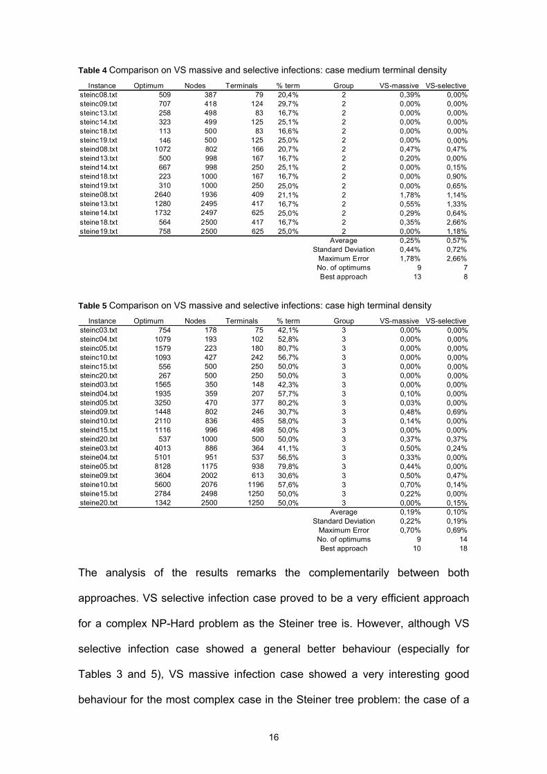
Table 4 Comparison on VS massive and selective infections: case medium terminal density

Instance Optimum Nodes Terminals % term Group VS-massive VS-selectivesteinc08.txt 509 387 79 20,4% 2 0,39% 0,00%steinc09.txt 707 418 124 29,7% 2 0,00% 0,00%steinc13.txt 258 498 83 16,7% 2 0,00% 0,00%steinc14.txt 323 499 125 25,1% 2 0,00% 0,00%steinc18.txt 113 500 83 16,6% 2 0,00% 0,00%steinc19.txt 146 500 125 25,0% 2 0,00% 0,00%steind08.txt 1072 802 166 20,7% 2 0,47% 0,47%steind13.txt 500 998 167 16,7% 2 0,20% 0,00%steind14.txt 667 998 250 25,1% 2 0,00% 0,15%steind18.txt 223 1000 167 16,7% 2 0,00% 0,90%steind19.txt 310 1000 250 25,0% 2 0,00% 0,65%steine08.txt 2640 1936 409 21,1% 2 1,78% 1,14%steine13.txt 1280 2495 417 16,7% 2 0,55% 1,33%steine14.txt 1732 2497 625 25,0% 2 0,29% 0,64%steine18.txt 564 2500 417 16,7% 2 0,35% 2,66%steine19.txt 758 2500 625 25,0% 2 0,00% 1,18%



Table 5 Comparison on VS massive and selective infections: case high terminal density

Instance Optimum Nodes Terminals % term Group VS-massive VS-selectivesteinc03.txt 754 178 75 42,1% 3 0,00% 0,00%steinc04.txt 1079 193 102 52,8% 3 0,00% 0,00%steinc05.txt 1579 223 180 80,7% 3 0,00% 0,00%steinc10.txt 1093 427 242 56,7% 3 0,00% 0,00%steinc15.txt 556 500 250 50,0% 3 0,00% 0,00%steinc20.txt 267 500 250 50,0% 3 0,00% 0,00%steind03.txt 1565 350 148 42,3% 3 0,00% 0,00%steind04.txt 1935 359 207 57,7% 3 0,10% 0,00%steind05.txt 3250 470 377 80,2% 3 0,03% 0,00%steind09.txt 1448 802 246 30,7% 3 0,48% 0,69%steind10.txt 2110 836 485 58,0% 3 0,14% 0,00%steind15.txt 1116 996 498 50,0% 3 0,00% 0,00%steind20.txt 537 1000 500 50,0% 3 0,37% 0,37%steine03.txt 4013 886 364 41,1% 3 0,50% 0,24%steine04.txt 5101 951 537 56,5% 3 0,33% 0,00%steine05.txt 8128 1175 938 79,8% 3 0,44% 0,00%steine09.txt 3604 2002 613 30,6% 3 0,50% 0,47%steine10.txt 5600 2076 1196 57,6% 3 0,70% 0,14%steine15.txt 2784 2498 1250 50,0% 3 0,22% 0,00%steine20.txt 1342 2500 1250 50,0% 3 0,00% 0,15%



The analysis of the results remarks the complementarily between both

approaches. VS selective infection case proved to be a very efficient approach

for a complex NP-Hard problem as the Steiner tree is. However, although VS

selective infection case showed a general better behaviour (especially for

Tables 3 and 5), VS massive infection case showed a very interesting good

behaviour for the most complex case in the Steiner tree problem: the case of a

17

medium density of terminals. Within this range of comparison the massive

approach outperformed the selective one. Furthermore, the massive infection

approach maintained a bounded distribution of its standard deviation, which

provides a better adjustment around the optimum. It also provided the best

solution for all the problems except for C8 (0.39% error versus 0.00%), D13

(0.20% versus 0.00%) and E8 (1.78% versus 1.14%).

5. Illustration: the Variable job Scheduling Problem (VSP)

We make use of the variable job scheduling problem to illustrate the VS

methodology. Initially, we are representing the virus evolution for a selective

infection case.

The Variable job Scheduling Problem (VSP) (see Gertsbakh and Stern, 1978;

Gabrel, 1995; and Wolfe and Sorensen, 2000 for relevant references), is

characterized as the problem of scheduling, on a set of parallel machines, a

number of non-preemptive jobs, each with a time interval for its processing. For

a fixed number of machines, the objective is maximizing the weighted number

of jobs processed, assuming a weight for each job. VSP is NP-Complete in all

of the cases (Kovalyov and Cheng, 2007). On the other hand, it is also possible

to consider a tactical objective that calculates the number of machines

necessary to process all jobs.

Figure 5 presents an illustration of the problem considering 10 jobs. Between

parentheses we represent the weight of the job and the processing time

corresponds to the width of each rectangle. Square brackets represent the time

windows for the processing. For the problem we have 2 machines.

18

Figure 5 Illustration of the VSP

Next we are going to describe an illustration of the lytic and the lysogenic

replication. We could consider this illustration included in both, selective and

massive infection procedure.

For an iteration t, we could imagine a population as that showed in Table 6,

considering 5 cells. First column shows selected jobs and, between

parenthesis, machine that processes the job and its starting time instant. Cells

2, 4 and 5 have a lytic replication whereas for cells 1 and 3 the replication is

lysogenic.

Table 6 Population for the iteration t

19

5.1. Illustration lytic Replication

If the algorithm randomly selects cell 4 (Figure 6) to be replicated, and NR4

reaches LN4, we can illustrate the lytic process as follows.

0 5 10 15 20 25

M2 4(123)

3(105) 8(30)M1

Figure 6 Cell 4

For simplicity and since we are going to consider a short neighbourhood, we

calculate all neighbouring solutions of cell 4. To obtain the neighbourhood, we

define three moves: insertion, replacement and displacement.

5.1.1. Insertion

We try to insert jobs that are not in the solution of the cell. Figure 7 shows all

possible solutions with an insertion move.

20

Figure 7 Insertion moves

5.1.2. Replacement

We change each job in the solution for another that is not there. We give more

probability to jobs with a greater weight.

Figure 8 Replacement moves

5.1.3. Displacement

21

The last move inserts jobs through the movement of each job in the solution. As

the previous move, if more than one job can be inserted, we discriminate with

the weight of the job.

Figure 9 Displacement moves

After generating the neighbourhood (Figure 10), we arrange the list of

neighbouring solutions is descending order regarding solution health (Figure

11).

Figure 10 Neighbourhood

22

1(1,1) . 3(1,5) . 4(2,4) . 8(1,19)

0 0

2(1,2) . 3(1,5) . 4(2,4) . 8(1,19)

0 0

3(1,5) . 4(2,4) . 7(2,18) . 8(1,19)

0 0

3(1,5) . 4(2,4) . 8(1,19) . 10(1,23)

0 0

3(1,5) . 4(2,4) . 8(1,19) . 9(2,20)

0 0

4(2,4) . 5(1,10) . 8(1,19)

0 0

3(1,5) . 5(2,9) . 8(1,19)

0 03(1,5) . 4(2,4) . 9(1,20)

0 0

1(2,1) . 3(1,5) . 4(2,6) . 8(1,19)

0 0

3(1,3) . 4(2,4) . 5(1,12). 8(1,19)

0 0

jobs (m,k) NR IT fitness LNR LIT

323

308

275

301

328

235

217

298

323

340 0

0

0

0

0

0

0

0

0

0

0

0

0

0

0

0

0

0

0

0

Figure 11 Neighbourhood

Then, we try to replace the cell replicated with one of those solutions, starting

from the best solution. For the illustration, we assume that the method replace

the first one, i.e., the best solution.

Figure 12 New population

23

Randomly, we choice the new cell type for the cell replicated. LNR value for the

cell is calculated as (5):

0ˆ( ) ( )

ˆ( )xf x f xLNR LNR

f x−

=

( 5 )

where x̂ is the best cell so far, x is the new cell and LNR0 is the initial value for

LNR.

LITx is calculated in a similar way as (6):

0ˆ( ) ( )

ˆ( )xf x f xLIT LIT

f x−

= ( 6 )

To end the iteration, we check if the new solution generated is the best solution

found so far in order to update x̂ .

5.2. Illustration lysogenic replication

We suppose that a lysogenic cell is chosen to be replicated in the next iteration:

let cell 3 of the population (represented in Figure 13). We also suppose

.

Figure 13 Cell 3

24

We randomly select a job k. If job k is not in the solution, we try to insert job k in

the solution of cell 3. For example, if selected job is 9, we could insert it in

machine 2 (Figure 14).

Figure 14 Lysogenic Insertion

On the other hand, if job k belongs to the solution, then we try a replacement

move with job k, as in lytic replication. For example, if k = 4 , we can replace job

4 by job 3, as figure 15 shows.

Figure 15 Lysogenic replacement

If any job can replace job k, then we get a worse solution than the original,

because we extract to the solution job k in all of the cases.

As in the lytic replication, we randomly assign a replication type for the new cell

and calculate its new LIT or LNR.

Finally, we include a brief summary in Table 7 showing results of comparison

between selective infection virus and an implementation of a Tabu Search

approach that was created with the same definition of neighbourhood used for

the lytic replication. The numbers of iterations for VS was 10,000 and 1,000 for

25

Tabu Search, in order to spend similar processing times. The rest of parameters

of the algorithms were previously fixed in a suitable manner after calibration.

Table 7 Summary of results

Selective Virus Tabu Search Window

size Work Load Jobs Avg. Error

(%) Avg. Time

(sec) Avg. Error

(%) Avge. Time

(sec) [1,5] Low 25 0,38 4,50 1,60 3,00[1,5] Medium 25 0,00 5,40 1,02 1,90[1,5] High 25 0,00 5,80 2,46 2,60[1,10] Low 25 0,05 6,90 3,91 4,70[1,10] Medium 25 0,00 7,10 1,71 4,60[1,10] High 25 0,00 8,80 2,39 4,60[1,5] Low 50 1,98 5,50 5,39 11,40[1,5] Medium 50 0,65 9,60 3,93 14,40[1,5] High 50 0,51 11,20 3,40 14,80[1,10] Low 50 3,14 8,80 8,10 30,20[1,10] Medium 50 1,44 13,20 4,60 37,80[1,10] High 50 1,07 17,70 3,86 37,90[1,5] Low 100 3,97 31,90 8,67 51,90[1,5] Medium 100 3,07 44,60 7,09 83,80[1,5] High 100 2,03 62,30 5,77 95,80[1,10] Low 100 5,45 46,10 10,68 120,10[1,10] Medium 100 4,44 67,80 10,70 217,80[1,10] High 100 4,17 100,00 7,71 260,30

Windows size is the starting interval size for each job. They are uniformly and

randomly generated in the range [1,5] and [1,10]. Work load express the

number of jobs per instant of the time horizon. Low work load represents an 80-

90% of jobs processed; medium work load a 50-60%; and high work load a 25-

35%.

All instances have been solved by an optimizer, in order to obtain the optimal

solution and to be able to test the performance for both methods. Error

averages are taken over 10 instances generated for each tuple (Windows Size,

Work Load, and number of jobs). Average computational times are provided in

26

CPU seconds. We used Lingo Optimizer to get optimal solutions and calculate

average errors.

Computational results in Table 7 show how the VS selective implementation

provides better results for all the cases than Tabu Search. Also, regarding CPU

time, Tabu Search presents a worse behavior for, practically, all the instances.

6. Conclusions and further research

VSs have proven successful when dealing with network complex problems. Its

extension to other complex problems is promising and new papers dealing with

this novel bio-inspired approach should be expected in the scientific literature.

Future research could consider several aspects. First, as VS is still a novel field

of research VS could be applied to solve numerous computational complexity

problems, several of them well known in the scientific literature and

characterized as NP-Hard problems. However, one of the most challenging

approaches is to focus on testing new viruses different from phages to explore

their optimisation capabilities and particular behaviour. In fact, lytic and

lysogenic replication cycles of phagocytes correspond to the less complex virus

infection, and it is easy to think that more complex infection forms could lead to

more successful infection process. The goal would be the generation of an

optimisation library associated to different classes of viruses and capable of

adapting to each specific problem. However, this research will require a

previous detailed medical investigation to clearly characterize the different viral

processes, and multidisciplinary research teams would be very welcome.

27

7. References

Beasley J.E. 2008: OR-Library. URL:

http://people.brunel.ac.uk/~mastjjb/jeb/inf

o.html accessed 2010. Cortés P., García J.M., Muñuzuri J. and

Guadix J. 2010: A Viral System massive

infection algorithm to solve the Steiner

tree problem in graphs with medium

terminal density. International Journal of

Bio-inspired Computation 4(2), in press.

Cortés P., García J.M., Muñuzuri J. and Onieva L. 2008: Viral Systems: a new

bio-inspired optimisation approach.

Computers & Operations Research 35(9),

2840-2860.

Cutello V., Nicosia G. and Pavone M. 2007: An Immune Algorithm with

Stochastic Aging and Kullback Entropy

for the Chromatic Number Problem.

Journal of Combinatorial Optimization 14

(1), 9-33.

Cutello V., Nicosia G., Pavone M. and Timmis J. 2007: An Immune Algorithm

for Protein Structure Prediction on Lattice

Models. IEEE Transaction on

Evolutionary Computation 11(1), 101-117.

Gabrel V. 1995: Scheduling jobs within

time windows on identical parallel

machines: New model and algorithms.

European Journal of Operational

Research, 83, pp. 320-329.

Gertsbakh I. and Stern H. 1978: Minimal

Resources for Fixed and Variable Job

Schedules. Operations Research, 26 (1),

68-85.

Kovalyov M, Ng C. Cheng T. 2007: Fixed

interval scheduling: Models, applications,

computacional complexity and algorithms.

European Journal of Operational

Research 178, 331-342.

Kubota, N., Fukuda, T., Shimojima, K. 1996: Virus-evolutionary genetic

algorithm for a self-organizing

manufacturing system. Computers and

Industrial Engineering 30 (4), 1015-1026.

Saito, S. 2003: A Genetic Algorithm by Use

of Virus Evolutionary Theory for

Combinatorial Problems. Optimization

and Optimal Control, Vol.1, World

Scientific Publishing Co.; 10: 251-268.

Van Dyke Parunak H. 1997: Go to the ant:

Engineering principles from natural multi-

agent systems. Annals of Operations

Research 75, 69-101.

Wolfe, W.J. and Sorensen, S.E. 2000:

Three scheduling algorithms applied to

Earth Observing systems domain.

Management Science, 46, 148-168.

Documents

Viral system algorithm: foundations and comparison between