VILNIUS UNIVERSITY

ANDRIUS ŠKARNULIS

QUADRATIC ARCH MODELS WITH LONG MEMORY AND QML

ESTIMATION

Doctoral DissertationPhysical Sciences, Mathematics (01 P)

Vilnius, 2017

The dissertation was written in 2012–2016 at Vilnius University.

Scientific Supervisor – Prof. Dr. Habil. Donatas Surgailis (Vilnius Uni-versity, Physical Sciences, Mathematics – 01 P).

Scientific Adviser – Prof. Dr. Habil. Remigijus Leipus (Vilnius University,Physical Sciences, Mathematics – 01 P).

VILNIAUS UNIVERSITETAS

ANDRIUS ŠKARNULIS

KVADRATINIAI ILGOSIOS ATMINTIES ARCH MODELIAI IR

PARAMETRU VERTINIMAS KVAZIDIDŽIAUSIO TIKETINUMO

METODU

Daktaro disertacijaFiziniai mokslai, matematika (01 P)

Vilnius, 2017

Disertacija rengta 2012–2016 metais Vilniaus universitete.

Mokslinis vadovas – prof. habil. dr. Donatas Surgailis (Vilniaus uni-versitetas, fiziniai mokslai, matematika – 01 P).

Mokslinis konsultantas – prof. habil. dr. Remigijus Leipus (Vilniausuniversitetas, fiziniai mokslai, matematika – 01 P).

Acknowledgements

First and foremost, I would like to express my sincere gratitude to my

scientific supervisor Prof. Donatas Surgailis for his inspiration, patient

mentoring and all the support and help during the years of my PhD stud-

ies. Without his active involvement, immense knowledge and guidance it

would be hard to imagine the results of this dissertation as they are. Also

a very special thanks goes to Prof. Liudas Giraitis for his helpful advice,

encouragement, thought-provocing discussions and the opportunity to

participate in joint work on interesting topics. It has been a great privilege

and honor to learn from some of the brightest figures in the field of math-

ematics. I would also like to thank my loving parents, brother and my

fiancée Ugne for their support and understanding through all these years.

Andrius Škarnulis

Vilnius

April 10, 2017

v

Table of Contents

Notations and Abbreviations ix

1 Introduction 1

2 Background 72.1 Definitions and preliminaries . . . . . . . . . . . . . . . . . 72.2 Long memory . . . . . . . . . . . . . . . . . . . . . . . . . . 142.3 Estimation . . . . . . . . . . . . . . . . . . . . . . . . . . . . 18

3 Stationary integrated ARCH(∞) and AR(∞) processes with fi-nite variance 263.1 Introduction . . . . . . . . . . . . . . . . . . . . . . . . . . . 273.2 Stationary solutions of FIGARCH, IARCH and ARCH equa-

tions . . . . . . . . . . . . . . . . . . . . . . . . . . . . . . . . 343.3 Stationary Integrated AR(∞) processes: Origins of long

memory . . . . . . . . . . . . . . . . . . . . . . . . . . . . . 423.4 Proofs of Theorem 3.1 and Corollaries 3.1-3.4 . . . . . . . . 503.5 Proofs of Theorems 3.2 and 3.3 . . . . . . . . . . . . . . . . 553.6 Simulation study . . . . . . . . . . . . . . . . . . . . . . . . 61

3.6.1 FIGARCH and ARFIMA(0,d,0) processes . . . . . . 613.6.2 IAR(p, d, q) and ARFIMA(p, d, q) processes . . . . 69

3.7 Conclusion . . . . . . . . . . . . . . . . . . . . . . . . . . . . 79

4 Quasi-MLE for the quadratic ARCH model with long memory 804.1 Introduction . . . . . . . . . . . . . . . . . . . . . . . . . . . 814.2 Stationary solution . . . . . . . . . . . . . . . . . . . . . . . 844.3 QML Estimators . . . . . . . . . . . . . . . . . . . . . . . . . 864.4 Main results . . . . . . . . . . . . . . . . . . . . . . . . . . . 894.5 Simulation study . . . . . . . . . . . . . . . . . . . . . . . . 934.6 Proofs . . . . . . . . . . . . . . . . . . . . . . . . . . . . . . . 964.7 Conclusion . . . . . . . . . . . . . . . . . . . . . . . . . . . . 111

vii

TABLE OF CONTENTS

5 A generalized nonlinear model for long memory conditionalheteroscedasticity 1125.1 Introduction . . . . . . . . . . . . . . . . . . . . . . . . . . . 1135.2 Stationary solution . . . . . . . . . . . . . . . . . . . . . . . 1155.3 Long memory . . . . . . . . . . . . . . . . . . . . . . . . . . 1335.4 Leverage . . . . . . . . . . . . . . . . . . . . . . . . . . . . . 138

6 Conclusions 142

Bibliography 144

viii

Notations and

Abbreviations

The following notations and abbreviations are used throughout the disser-

tation:

Z set of integers

N set of positive integers

R := (−∞,∞) set of real numbers

R+ set of positive real numbers

C set of complex numbers

:= "by definition"

L backshift operator (LXk = Xk−1)

[s] integer part of s

Var(Xk) variance of a random variable Xk

an ∼ bn if an/bn → 1, n→∞

C generic constant

‖·‖ the norm (of function or sequence)

d long memory parameter

Θ set of model parameters

ix

Notations and Abbreviations

θn estimator of θ ∈ Θ given infinite past (using the

unobserved process)

θn estimator of θ ∈ Θ given finite past (using the

observed process only)

Π := [−π, π]

i.i.d. independent identically distributed

B(t) standard Brownian motion

Bd+1/2(t) fractional Brownian motion

ζk, ξk, εk usually random "noise" of the process

→D[0,1] weak convergence in the Skorohod space D[0, 1]P→ convergence in probabilitya.s.→ almost sure convergenced→ convergence in distribution

Γ(·) Gamma function

B(·, ·) Beta function

E(Xk) mean of a random variable Xk

cov(·, ·), γ(·) covariance function of a random process

corr(·, ·), ρ(·) correlation function of a random process

∂x derivative with respect to variable x

a.e. almost everywhere

r.h.s. right-hand side

l.h.s. left-hand side

w.r.t. with respect to

r.v. random variable

RMSE root mean square error

QMLE quasi-maximum likelihood estimation (estimator)

x

Notations and Abbreviations

ARCH process Autoregressive Conditionally Heteroscedastic

process

LARCH process Linear ARCH process

GQARCH process Generalized Quadratic ARCH process

All (in)equalities involving random variables in this dissertation are sup-

posed to hold almost surely.

xi

Chapter 1

Introduction

Nowadays the importance of data and information that derives from it is

undeniable and grows rapidly. As time passes, scientists, corporations,

government institutions and others have the possibility to deal with longer

and longer time series of data. It is important to have adequate tools that

would allow us to analyze, model and forecast data retrieved from long

time series. In view of the importance of economics and financial markets

for today’s well-being, scientists developed a variety of statistical methods

that help better understand the dynamics and behavior of various financial

and economic indicators, as well as financial markets and economics in

general. It is commonly known that the dynamics of financial markets is

dynamical in itself, i.e. the volatility changes over time. However, this

important feature – referred to as "conditional heteroscedasticity" in the

context of time series – was often dismissed or ignored in many statistical

settings and modeling. Robert F. Engle won the 2003 Sveriges Riksbank

prize in Economic Sciences in Memory of Alfred Nobel "for methods of

analyzing economic time series with time-varying volatility (ARCH)". The

1

1. Introduction

parametric ARCH model, introduced by Engle [24] in 1982,

rt = ζtσt, σ2t = ω +

q∑j=1

bjr2t−j, t ∈ Z,

where ζt, t ∈ Z is an i.i.d. noise with zero mean and unit variance,

was extended in 1986 by Bollerslev [10] to the well-known GARCH(p, q)

process rt = ζtσt with conditional variance

σ2t = ω +

q∑j=1

bjr2t−j +

p∑j=1

ajσ2t−j.

The concept of autoregressive conditionally heteroscedastic models is

widepsread in theory on time series and practical applications.

Later on, parametric models were extended to include information

from infinite past, for example, in 1991 Robinson [62] introduced the

ARCH(∞) process whose conditional variance has the form

σ2t = ω +

∞∑j=1

bjr2t−j.

In the case of the GARCH(p, q) model, autocovariances decay exponen-

tially fast, ARCH(∞) may have autocovariances decaying to zero at a

slower rate, however, in these traditional settings, the stationary solution

with finite variance has summable autocovariances:∑

k∈Z γ(k) <∞ (ex-

cept, as we prove in this dissertation, in the case of ARCH(∞) with ω = 0

and∑∞

j=1 bj = 1), or covariance short memory, which is a major drawback

of similar models in light of the well-known phenomenon of long memory

in, for example, squared financial returns. As there is a need for new

models and there are still important unresolved problems in terms of

2

models that gained popularity in practical applications (e.g. FIGARCH),

the topic of long memory conditionally heteroscedastic time series is im-

portant, relevant and interesting in itself. The present dissertation focuses

on specific ARCH-type models with long memory, as well as the long

memory "generating mechanism", from which long memory originates in

the ARCH setting. In terms of practical applications, questions related to

parameter estimation for long memory models are also under the scope

of this dissertation.

The main aims set and problems raised in this dissertation are as

follows.

Finding conditions for the existence of a finite variance stationary solution

with long memory of FIGARCH, ARCH(∞) and integrated AR(∞) processes

(Chapter 3). The main goal is to find the necessary and sufficient conditions

for the existence of a stationary solution of the integrated ARCH(∞)

process, in particular, the so-called FIGARCH equation, proposed by

Baillie, Bollerslev and Mikkelsen [3] in 1996 to capture the long memory

effect in volatility. There is much discussion on controversies surrounding

the FIGARCH equation. In 1996 Ding and Granger [20] introduced the

LM(d)-ARCH model, whose important particular case is the FIGARCH

equation. They argued that a stationary solution of the LM(d)-ARCH

equation with the finite fourth moment has a long memory, however, the

existence of such a solution was never shown. By finding the above-

mentioned conditions for the existence of a stationary solution, we solve

the long standing Ding and Granger conjecture. We also aim to explore

the relation between the stationary solutions of ARCH(∞) (as well as

FIGARCH) and integrated AR(∞) processes – the stationary solution of

the former process is constructed in terms of the solution of the latter.

3

1. Introduction

Questions surrounding the IAR(∞) model are of independent interest.

The class of stationary IAR(∞) processes with long memory is vast and,

as our simulations show, its special case of IAR(p, d, q) models might

be reasonably considered as a new class of long memory models which

provides more flexibility to model long memory processes changing their

autocovariances on low lags without an effect on the long-term behavior.

Exploring the parametric quasi-maximum likelihood estimation for a new

generalized quadratic ARCH (GQARCH) process (Chapter 4). The Quadratic

ARCH (QARCH) process with long memory, introduced by Doukhan et al.

[22], and generalized in Chapter 5 of this dissertation (see also Grublyte

and Škarnulis [40]), extends the QARCH model of Sentana [66] and the

Linear ARCH (LARCH) model of Robinson [62] to the strictly positive

conditional variance. The GQARCH and LARCH models have similar

long memory and leverage properties and can both be used to model fin-

ancial data with these properties. The main disadvantage of the LARCH

model in comparison to the GQARCH model is the fact that volatility

in the case of LARCH may assume negative values and is not separated

from below by positive constant. The standard quasi-maximum likelihood

(QML) approach to the estimation of LARCH parameters is inconsistent.

We aim to investigate the QML estimation for the 5-parametric GQARCH

model, whose parametric form of moving average coefficients is the same

as that by Beran and Schützner [5] for the LARCH model. Our main goal

is to prove the consistency and asymptotic normality of the correspond-

ing estimates, including long memory parameter 0 < d < 1/2. Also, a

simulation study to evaluate the finite sample performance of the QML

estimation for GQARCH model is performed.

Investigating the existence and properties of a stationary solution of the gen-

4

eralized nonlinear model for long memory conditional heteroscedasticity (Chapter

5). As a parametric ARCH(q) model of Engle [24] was generalized to

GARCH(p, q) by Bollerslev [10], we aim to extend the ARCH-type model

discussed by Doukhan, Grublyte and Surgailis [22] to the model where

conditional variance satisfies an AR(1) equation σ2t = Q2(a+

∑∞j=1 bjrt−j)+

γσ2t−1 with a Lipschitz function Q(x).

The novelty of the results in this dissertation:

• conditions for the existence of the stationary finite variance solution

of integrated ARCH(∞) and FIGARCH processes with long memory.

• the final answer to the long standing conjecture of Ding and Granger

[20] about the existence of a stationary solution of the Long Memory

ARCH (as well as FIGARCH) model with long memory and the finite

fourth moment.

• introduction and investigation of a new class of long memory integ-

rated AR(p, d, q) processes, whose autocovariance can be modeled

easily at low lags without a significant effect on the long memory be-

havior, this being a major advantage over classical ARFIMA models.

• proof of consistency and asymptotic normality of the QML estimator

for the Generalized Quadratic ARCH process, empirical evaluation

of the finite sample performance of the QML estimation for the

GQARCH model.

• conditions for the existence of a stationary finite variance solution

of the generalized nonlinear model for long memory conditional

heteroscedasticity, its long memory and leverage properties.

Publications and conferences. The following three papers cover the main

results presented in this dissertation:

5

1. Introduction

• L. Giraitis, D. Surgailis and A. Škarnulis. Stationary integrated

ARCH(∞) and AR(∞) processes with finite variance. Submitted,

2017.

• I. Grublyte, D. Surgailis and A. Škarnulis. QMLE for quadratic

ARCH model with long memory. Journal of Time Series Analysis. 2016.

doi: 10.1111/jtsa.12227.

• I. Grublyte and A. Škarnulis. A nonlinear model for long memory

conditional heteroscedasticity. Statistics. 51:123–140, 2017.

The main results of this dissertation were also presented at the following

conferences:

• 8th International Conference of the ERCIM WG on Computational

and Methodological Statistics/9th International Conference on Com-

putational and Financial Econometrics, University of London, 12–14

December, 2015. Title of presentation: Quasi-MLE for quadratic ARCH

model with long memory.

• NBER-NSF Time Series Conference, Vienna University of Economics

and Business, 25–26 September, 2015. Title of presentation: Integrated

AR and ARCH processes and the FIGARCH model: origins of long memory.

• 11th International Vilnius Conference on Probability Theory and

Mathematical Statistics, Vilnius University, 29 June–1 July, 2014. Title

of presentation: An autoregressive conditional duration model and the

FIGARCH equation.

6

Chapter 2

Background

In Section 2.1 of this chapter we provide some basic definitions and pro-

positions, which will be used throughout the dissertation. Long memory,

as an object and important thematic line of this dissertation, will be briefly

described in Section 2.2. We touch upon the main principles of the para-

meter estimation for time series models in Section 2.3.

2.1 Definitions and preliminaries

Since the main interest of this dissertation lies in conditionally hetero-

scedastic models, first we recall that a time series Xk, k ∈ Z is called

conditionally homoscedastic if its conditional variance

σ2k = Var (Xk | Xk−1, Xk−2, ...) = C, k ∈ Z,

is constant, while in terms of conditionally heteroscedastic time series, its

conditional variance is a random process (in general). In this disserta-

tion, the term "stationary process" is mostly used by means of covariance

7

2. Background

stationarity.

Definition 2.1. Random process Xk, k ∈ Z is called covariance stationary if

EXk = C and EX2k <∞ are constant for all k ∈ Z, and the covariance function

cov(Xk, Xk+j) = cov(X0, Xj),

is constant in k, for all k, j ∈ Z.

As it will be stated in Section 2.2 of this chapter, the main instruments

we use (in this dissertation) to characterize the long memory property

of time series are the covariance and spectral density functions. Propos-

ition 2.1 below describes the relation between the covariance function,

spectral distribution function and spectral density. Suppose that function

F : [−π, π] → [0,∞) is right-continuous, nondecreasing, bounded and

F (−π) = 0.

Proposition 2.1. Function γ(k), k ∈ Z, is a covariance function of some sta-

tionary process if and only if

γ(k) =

∫ π

−πeiksdF (s),

with some (unique) function F , which is called a spectral distribution function.

If F (s) =∫ sπ f(ν)dν, then f is called a spectral density function.

The concept of a transfer function is used to prove important results

of this dissertation (Chapter 3).

Definition 2.2. Suppose that process Xk, k ∈ Z can be written as

Xk =∞∑j=0

ajZk−j, k ∈ Z,

8

2.1. Definitions and preliminaries

where Zk, k ∈ Z is a stationary process. Then the Fourier transform A(x) :=∑∞k=0 e

−ixkak, x ∈ Π, is called the transfer function.

Being the main object of this dissertation, the ARCH(∞) process is

defined as follows.

Definition 2.3. A nonnegative random process τk, k ∈ Z is said to satisfy

an ARCH(∞) equation if there exists a sequence of nonnegative i.i.d. random

variables εk, k ∈ Z with unit mean Eε0 = 1, a nonnegative number ω ≥ 0

and a deterministic sequence bj ≥ 0, j = 1, 2, . . . , such that

τk = εk

(ω +

∞∑j=1

bjτk−j

), k ∈ Z. (2.1)

In this dissertation, we assume that ARCH-type processes τk, k ∈ Z

(or rk, xk, depending on notation in a particular context) are causal, i.e.

for any k, τk can be represented as a measurable function f(εk, εk−1, . . . )

of the present and past values of innovations εs, s ≤ k. For example,

if stationarity and causality are not required, equation (2.1) can have

infinitely many solutions (see, e.g., Leipus and Kazakevicius [51]).

Definition 2.4. Let εk, k ∈ Z be a process of uncorrelated random variables

with zero mean and variance σ2ε . Then a random process Xk, k ∈ Z is said to be

causal with respect to εk, k ∈ Z if Xk = f(εk, εk−1, ...) for every k ∈ Z, where

f is a measurable function such that Xk is a properly defined random variable.

An important statistical concept, which will be assigned to many pro-

cesses considered in this dissertation, is ergodicity. To put in a simple

manner, this feature allows estimating the characteristics of a random pro-

cess, having only one sufficiently long realization of the process, without

9

2. Background

the need of using multiple independent samples. One often refers to

ergodicity for the mean, in which case:

1

n

n∑k=1

Xk → E(X0) = µ, n→∞.

A random process Xk, k ∈ Z is said to be ergodic for the second moment

if1

n− j

n∑k=j+1

(Xk − µ)(Xk−j − µ)P→ γ(j), for all j,

where γ(j) = cov(Xk, Xk−j) (see, e.g., Hamilton [43]). One can define an

ergodic process in a wider sense (see, e.g., Andersen and Moore [2]): a

random process Xk, k ∈ Z is ergodic if for any suitable function f(·) the

following limit exists almost surely:

E [f(X0)] = limN→∞

1

2N + 1

N∑k=−N

f(Xk).

Now we provide a more formal definition of a stationary ergodic time

series (see Lindner [54]).

Definition 2.5. Let Xk, k ∈ Z be a stationary time series of random variables

Xk in R. Then Xk, k ∈ Z can be seen as a random element in RZ, equipped

with its Borel-σ-algebra B(RZ). Let the backshift operator Φ : RZ → RZ be given

by Φ(zi, i ∈ Z) = zi−1, i ∈ Z. Then the time series Xk, k ∈ Z is called

ergodic if, for Λ ∈ B(RZ), Φ(Λ) = Λ implies P (Xk, k ∈ Z ∈ Λ) ∈ 0, 1.

The following proposition about the ergodicity of a random process is a

simplified version of Theorem 3.5.8 by Stout [67] and states that a meas-

urable function of an ergodic process forms again an ergodic process.

10

2.1. Definitions and preliminaries

Proposition 2.2. Suppose Xk, k ∈ Z is an ergodic sequence (e.g. i.i.d. ran-

dom variables) and f : R∞ → R is a measurable function. Then the sequence

Yk, k ∈ Z, where

Yk = f(Xk, Xk−1, ...),

is an ergodic process.

Since convergence in mean-square is almost without exception used in

the definitions of stationary solutions of many models in this dissertation,

we give a short definition for this mode of convergence.

Definition 2.6. We say that the sequence Xk, k ∈ Z of square integrable ran-

dom variables converges in mean-square if there exists a square integrable random

variable X such that

limk→∞

E[(Xk −X)2

]= 0.

In this dissertation, phrases "converges in L2" and "converges in mean-

square" are used interchangeably. Similarly to Definition 2.6, one could

define the convergence in Lp.

As discussed in Chapter 3 of this dissertation, the stationary solution

of the ARCH(∞) process can be constructed in terms of the discrete time

infinite Volterra series. For example, we show that the stationary solution

of ARCH(∞) process can be written in the form of causal Volterra series:

Yk = µ+ (2.2)

+ µσ

( ∞∑m=1

∑−∞<sm<···<s1≤k

gk−s1hs1−s2 · · ·hsm−1−smζs1 · · · ζsm

), k ∈ Z,

with standardized i.i.d. innovations ζk, k ∈ Z. In order to correctly

define the convergence of the discrete time infinite Volterra series (e.g.

11

2. Background

having the form (2.2)), we first remind a few facts and definitions related

to the summability in Banach spaces (see, e.g., Hunter and Nachtergaele

[45]). First, recall that a normed linear space is a metric space with respect

to metric d derived from its norm, where d(x, y) = ‖x− y‖. A Banach

space is a normed linear space that is a complete metric space with respect

to the metric derived from its norm.

Definition 2.7. Let xi, i ∈ I be an indexed set in a Banach space E, where I

is a countable index set. For each finite subset J of I , we define the partial sum

SJ by

SJ =∑i∈J

xi.

We say that x ∈ E is a sum of an indexed set xi, i ∈ I if for every ε > 0 there

is a finite subset J ε of I such that ‖SJ − x‖ < ε for all finite subsets J of I that

contain J ε.

Definition 2.8. If x ∈ E is the sum of an indexed set xi, i ∈ I (in the sense

of Definition 2.7), then we write x =∑

i∈I xi, and the set xi, i ∈ I is called

summable.

The fact that the set in a Banach space is summable ensures many useful

features, for example, the possibility to change the summation order, etc.

Recall that the set U of vectors in a Hilbert space H is orthonormal if

it is orthogonal, i.e. for every x, y ∈ U we have 〈x, y〉 = 0, and ‖x‖ = 1

for all x ∈ U . Let I be the same countable index set as in Definitions 2.7

and 2.8 above, ei, i ∈ I – some orthonormal set in a Hilbert space H

(in particular, in an L2 space), and ci, i ∈ I the set of real numbers. It

is known that the square summability of ci, i.e.∑

i c2i < ∞, guarantees

that the set ciei, i ∈ I is summable in space H (in particular, in space L2).

12

2.1. Definitions and preliminaries

The last fact is especially useful when thinking about the convergence

(in L2) of the discrete time infinite Volterra series (e.g. having the form

(2.2)). Indeed, since ζk, k ∈ Z in (2.2) is the sequence of independent

and identically distributed standardized random variables, then for each

k ∈ Z the set ζs1 · · · ζsm,m ≥ 1, sm < ... < s1 ≤ k ∈ Z is orthonormal in

L2. In this case, the convergence of Volterra series mainly depends on

its coefficients – if they are square summable (which is ensured by our

assumptions, see Chapter 3), the Volterra series converges in L2. We also

note that if variables Xk are nonnegative, then from the summability of∑k∈ZXk in the L2 space follows the almost sure convergence of this series.

Next we define two classes of processes – bilinear and linear ARCH

– which will act as important models in the three main chapters of this

dissertation, especially Chapter 3, for the construction of a stationary

solution for the IARCH(∞) process. ARCH-type bilinear models where

considered by, for example, Giraitis and Surgailis [30].

Definition 2.9. We say that the discrete stationary process Xk, k ∈ Z satisfies

the bilinear equation (or is a bilinear process) if

Xk = ζk

(a+

∞∑j=1

ajXk−j

)+ b+

∞∑j=1

bjXk−j, (2.3)

where ζk, k ∈ Z is a sequence of i.i.d. random variables with Eζk = 0 and

Var(ζk) = 1, a, aj, b, bj, j ≥ 1, are real coefficients. In the case of b = bj ≡ 0,

(2.3) is the Linear ARCH (LARCH) model introduced by Robinson [62].

We define the Brownian motion and the fractional Brownian motion,

following Giraitis et al. [36].

13

2. Background

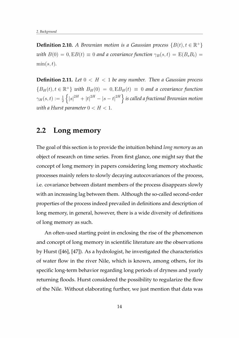
Definition 2.10. A Brownian motion is a Gaussian process B(t), t ∈ R+

with B(0) = 0,EB(t) ≡ 0 and a covariance function γB(s, t) = E(BsBt) =

min(s, t).

Definition 2.11. Let 0 < H < 1 be any number. Then a Gaussian process

BH(t), t ∈ R+ with BH(0) = 0,EBH(t) ≡ 0 and a covariance function

γH(s, t) := 12

|s|2H + |t|2H − |s− t|2H

is called a fractional Brownian motion

with a Hurst parameter 0 < H < 1.

2.2 Long memory

The goal of this section is to provide the intuition behind long memory as an

object of research on time series. From first glance, one might say that the

concept of long memory in papers considering long memory stochastic

processes mainly refers to slowly decaying autocovariances of the process,

i.e. covariance between distant members of the process disappears slowly

with an increasing lag between them. Although the so-called second-order

properties of the process indeed prevailed in definitions and description of

long memory, in general, however, there is a wide diversity of definitions

of long memory as such.

An often-used starting point in enclosing the rise of the phenomenon

and concept of long memory in scientific literature are the observations

by Hurst ([46], [47]). As a hydrologist, he investigated the characteristics

of water flow in the river Nile, which is known, among others, for its

specific long-term behavior regarding long periods of dryness and yearly

returning floods. Hurst considered the possibility to regularize the flow

of the Nile. Without elaborating further, we just mention that data was

14

2.2. Long memory

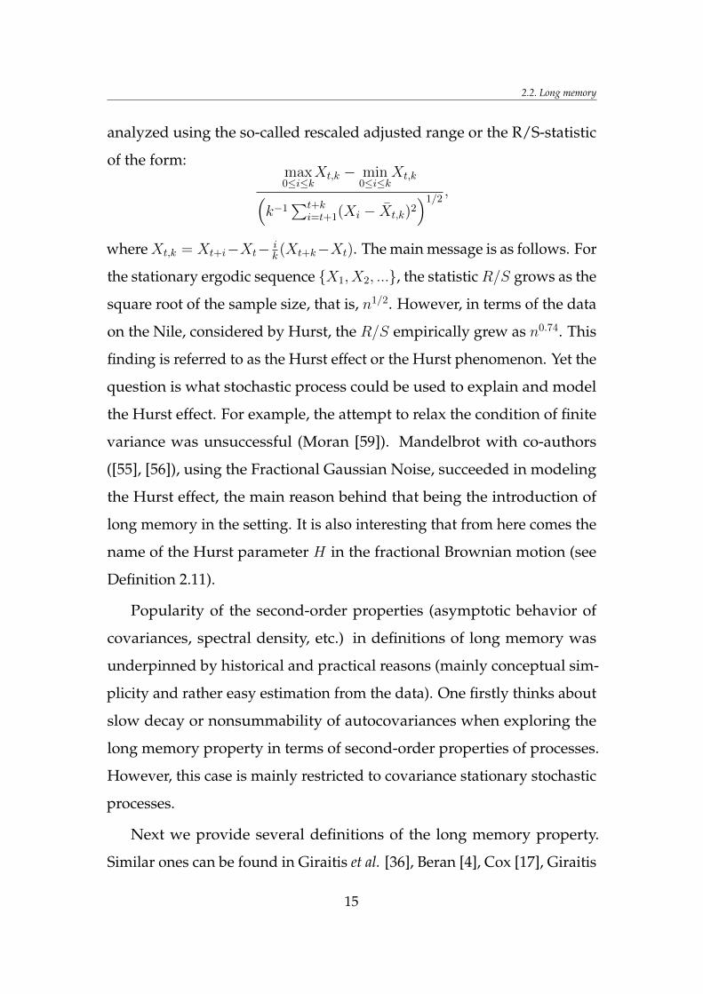
analyzed using the so-called rescaled adjusted range or the R/S-statistic

of the form:max0≤i≤k

Xt,k − min0≤i≤k

Xt,k(k−1

∑t+ki=t+1(Xi − Xt,k)2

)1/2,

whereXt,k = Xt+i−Xt− ik(Xt+k−Xt). The main message is as follows. For

the stationary ergodic sequence X1, X2, ..., the statisticR/S grows as the

square root of the sample size, that is, n1/2. However, in terms of the data

on the Nile, considered by Hurst, the R/S empirically grew as n0.74. This

finding is referred to as the Hurst effect or the Hurst phenomenon. Yet the

question is what stochastic process could be used to explain and model

the Hurst effect. For example, the attempt to relax the condition of finite

variance was unsuccessful (Moran [59]). Mandelbrot with co-authors

([55], [56]), using the Fractional Gaussian Noise, succeeded in modeling

the Hurst effect, the main reason behind that being the introduction of

long memory in the setting. It is also interesting that from here comes the

name of the Hurst parameter H in the fractional Brownian motion (see

Definition 2.11).

Popularity of the second-order properties (asymptotic behavior of

covariances, spectral density, etc.) in definitions of long memory was

underpinned by historical and practical reasons (mainly conceptual sim-

plicity and rather easy estimation from the data). One firstly thinks about

slow decay or nonsummability of autocovariances when exploring the

long memory property in terms of second-order properties of processes.

However, this case is mainly restricted to covariance stationary stochastic

processes.

Next we provide several definitions of the long memory property.

Similar ones can be found in Giraitis et al. [36], Beran [4], Cox [17], Giraitis

15

2. Background

and Surgailis [30], Giraitis et al. [35].

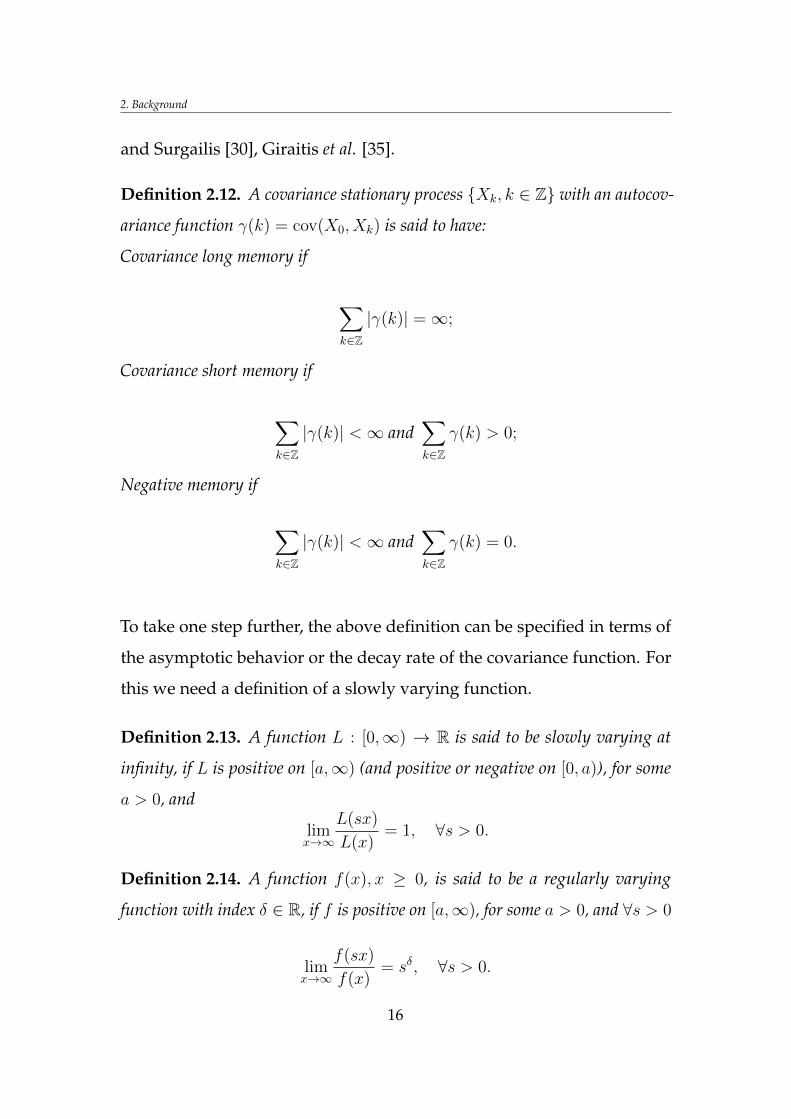
Definition 2.12. A covariance stationary process Xk, k ∈ Z with an autocov-

ariance function γ(k) = cov(X0, Xk) is said to have:

Covariance long memory if

∑k∈Z

|γ(k)| =∞;

Covariance short memory if

∑k∈Z

|γ(k)| <∞ and∑k∈Z

γ(k) > 0;

Negative memory if

∑k∈Z

|γ(k)| <∞ and∑k∈Z

γ(k) = 0.

To take one step further, the above definition can be specified in terms of

the asymptotic behavior or the decay rate of the covariance function. For

this we need a definition of a slowly varying function.

Definition 2.13. A function L : [0,∞) → R is said to be slowly varying at

infinity, if L is positive on [a,∞) (and positive or negative on [0, a)), for some

a > 0, and

limx→∞

L(sx)

L(x)= 1, ∀s > 0.

Definition 2.14. A function f(x), x ≥ 0, is said to be a regularly varying

function with index δ ∈ R, if f is positive on [a,∞), for some a > 0, and ∀s > 0

limx→∞

f(sx)

f(x)= sδ, ∀s > 0.

16

2.2. Long memory

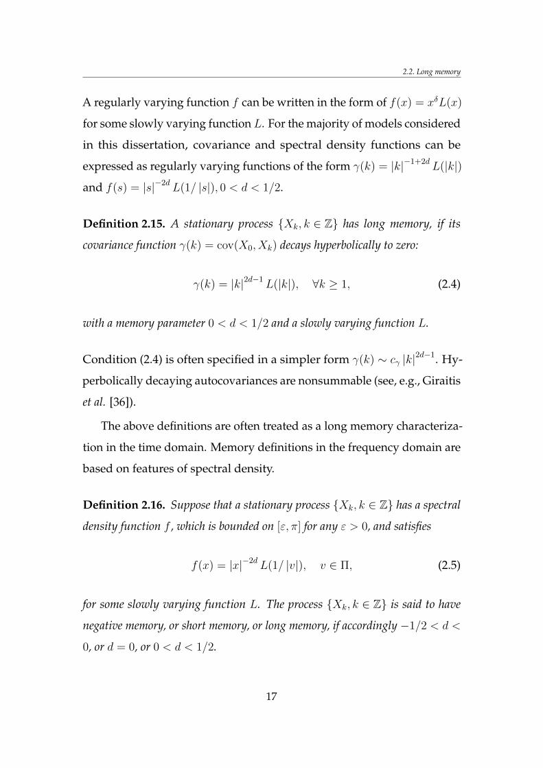
A regularly varying function f can be written in the form of f(x) = xδL(x)

for some slowly varying function L. For the majority of models considered

in this dissertation, covariance and spectral density functions can be

expressed as regularly varying functions of the form γ(k) = |k|−1+2dL(|k|)

and f(s) = |s|−2dL(1/ |s|), 0 < d < 1/2.

Definition 2.15. A stationary process Xk, k ∈ Z has long memory, if its

covariance function γ(k) = cov(X0, Xk) decays hyperbolically to zero:

γ(k) = |k|2d−1L(|k|), ∀k ≥ 1, (2.4)

with a memory parameter 0 < d < 1/2 and a slowly varying function L.

Condition (2.4) is often specified in a simpler form γ(k) ∼ cγ |k|2d−1. Hy-

perbolically decaying autocovariances are nonsummable (see, e.g., Giraitis

et al. [36]).

The above definitions are often treated as a long memory characteriza-

tion in the time domain. Memory definitions in the frequency domain are

based on features of spectral density.

Definition 2.16. Suppose that a stationary process Xk, k ∈ Z has a spectral

density function f , which is bounded on [ε, π] for any ε > 0, and satisfies

f(x) = |x|−2dL(1/ |v|), v ∈ Π, (2.5)

for some slowly varying function L. The process Xk, k ∈ Z is said to have

negative memory, or short memory, or long memory, if accordingly −1/2 < d <

0, or d = 0, or 0 < d < 1/2.

17

2. Background

Condition (2.5) is often simplified to f(x) ∼ cf |x|−2d, x → 0, with some

constant cf > 0.

Papers that investigate long memory processes, often alongside con-

sideration of the decay rate and summability of autocovariances, also

investigate the convergence of the partial sums process. This is yet an-

other way to define long memory.

Definition 2.17. We say that a strictly stationary process Xk, k ∈ Z has

distributional long memory if its normalized partial sums processA−1n

[ns]∑k=1

(Xk −Bn) : s ∈ [0, 1]

converges, in the sense of weak convergence of the finite dimensional distributions,

as n→∞, to a random process Z(s)s∈[0,1] with dependent increments. Here

An →∞, n→∞, and Bn are some constants .

There are many other types of definitions, however, we will not con-

sider them any further. In this dissertation, by long memory we mean the

covariance long memory, unless stated otherwise.

2.3 Estimation

The field of statistical procedures and methods to estimate parameters of

time series models can be a brigde between theory and practical applica-

tion. In this section, we briefly discuss and review the main methods used

to estimate parameters of conditionally heteroscedastic time series models,

not necessarily those with long memory. A variety of different ways was

introduced to estimate the time series models. The first two concepts that

18

2.3. Estimation

should be mentioned with reference to this topic are the Least Squares (LS)

method and the Quasi-maximum likelihood (QML) method. The former is

often called the simplest method to estimate parametric ARCH(q) models,

while the latter is particularly relevant for GARCH(p, q). For example,

for the strictly stationary GARCH process, the QML estimators are con-

sistent and asymptotically normal with no moment assumption on the

observed process, using some mild regularity conditions instead. This is

particularly important from a practical point of view as for many financial

time series the requirement of the finite fourth or even higher moments is

questionable. To provide the main idea behind LS and QML estimation,

we use the examples of parametric ARCH and GARCH models. Then

we will move on to discussing the case of infinite order models such as

ARCH(∞).

The basic idea behind the parameter estimation of the time series

model is as follows. Having a finite data set of size n, r1, ..., rn, we

assume that these observations come from a random process of a specific

form which often (but not always) depends on a finite number of para-

meters. In this section, we denote the true (unknown) values of these

parameters with θ0 = (θ01, ..., θ0p), p < ∞. The main goal is to get the

"best" estimates θn of θ0 from the data that we have. Here, the subscript n

indicates that we calculate the estimator using the available data sample

of size n. In most cases, different methods can be applied. Independently

of what we choose, two concepts (features), which are inevitably found in

the statistical inference and estimation literature, are a) consistency and

b) asymptotic normality of estimators. The estimator is called consist-

ent if θn → θ0 in probability as n → ∞. Strong consistency means that

the above-mentioned convergence holds almost surely. Most often by

19

2. Background

asymptotic normality we mean that the difference between the consist-

ent estimator θn and true parameters θ0 converges in distribution to the

normal distribution:

√n(θn − θ0)

d→ N(0, V ).

When θ0 ∈ Rp, then V is a p× p matrix.

The parametric ARCH(q) model is often used to explain how the Least

Squares (LS) method works (see, e.g., Francq and Zakoian [27], Francq

and Zakoian [28]). One of the reasons behind this is that, for ARCH(q),

the LS estimation provides estimators in the explicit form. Let’s consider

the process

rk = σkζk, σ2k = ω0 +

q∑j=1

a0jr2k−j, k ∈ Z, (2.6)

with ω0 > 0, a0i ≥ 0, i = 1, ..., q, and ζk, k ∈ Z an i.i.d. sequence with

zero mean and unit variance. The vector of true parameters is θ0 =

(ω0, a01, ..., a0q)T (T denotes the transposed vector). The LS estimation

procedure for ARCH(q) is performed rewriting (2.6) as an AR(q) equation

for r2k:

r2k = ω0 +

q∑j=1

a0jr2k−j + uk,

with uk = r2k − σ2

k = (ζ2k − 1)σ2

k. As usual in terms of estimation, we

try to estimate the model parameters from a finite sample of observed

values (r1, ..., rn), with the initial set of observations being (r0, ..., r1−q), all

of which can be, for example, zero-valued. The LS estimator is given by

θn = (ω, a1, ..., aq) = (XTX)−1XTY,

20

2.3. Estimation

where

Y = Xθ0 + U,

with

XT =

ZTn−1

...

ZT0

, Y =

r2n

...

r21

, U =

un...

u1

,

and vectors ZTk−1 = (1, r2

k−1, ..., r2k−q).

If rk, k ∈ Z is a nonanticipative strictly stationary solution of (2.6),

ω0 > 0 and Er2k <∞, then the LS estimator of σ2

0 = Var(uk) is

σ2 =1

n− q − 1

n∑t=1

(r2t − ω −

q∑j=1

ajr2t−j

)2

.

Strong consistency, that is,

θna.s.→ θ0, σ2

na.s.→ σ2

0,

can be achieved under Er4k <∞ and P(ζ2

k = 1) 6= 1, while for asymptotic

normality the finiteness of the eight moment is needed, Er8k <∞ (see, e.g.,

Bose and Mukherjee [11]), then

√n(θn − θ0)

d→ N(0, (Eζ4k − 1)A−1BA−1),

where A = E(ZqZTq ) and B = E(σ4

q+1ZqZTq ). Some "improvements" of the

ordinary LS method could be mentioned. For example, in the case of

linear regression, when model errors are heteroscedastic, the so-called

Feasible Generalized Least Squares (or Quasi-generalized Least Squares)

21

2. Background

estimation is asymptotically more accurate (see, e.g., Hamilton [43]). In

the latter case, the main difference appears to be the definition of the estim-

ator which is θ∗n = (XT ΩX)−1XT ΩY , with Ω = diag(σ−41 (θ1), ..., σ−4

n (θ1)).

Another important aspect is that ordinary LS estimation can produce

negative estimates of volatility – in order to avoid this problem the Con-

strained Least Squares estimation is used.

Next we present some basic aspects related to Quasi-maximum like-

lihood estimation (QMLE), which is without a doubt one of the most

popular choices for parameter estimation of time series models such as

GARCH, ARCH and others, including those with a long memory property.

The name of this method entails "quasi", because the likelihood function

we are maximizing to find the estimates of model parameters is written

under the assumption of normally distributed innovations of the pro-

cess. As it turns out, such an assumption is not critical for the asymptotic

behavior of the estimator.

Let us now turn to the GARCH process to illustrate the main idea of

QMLE. A number of papers consider the QMLE for GARCH processes,

see, e.g., Hall and Yao [42], Francq and Zakoian [26], Berkes et al. [8],

Berkes and Horváth [6], Berkes and Horváth [7]. The process we consider

is a strictly stationary solution of equations

rk = σkζk, σ2k = ω0 +

q∑j=1

a0jr2k−j +

p∑j=1

b0jσ2k−j, k ∈ Z. (2.7)

For estimation purposes, we assume that orders p and q are known. The

true (unknown) parameters of this model are

θ0 = (θ0,1, ..., θ0,p+q+1)T = (ω0, a01, ..., a0q, b01, ..., b0p)T .

22

2.3. Estimation

We want to estimate parameter θ0 from the available realization of (2.7):

r1, ..., rn, choosing the initial values of r0, ..., r1−q, σ20, ..., σ

21−p. One of the

possible choices of initial values is, for example, r20 = ... = r2

1−q = σ20 =

... = σ21−p = r2

1. Since we start the process from chosen initial values, which

affects the stationarity, further we work withσ2t

. The QML estimator of

θn is defined as

θn = arg maxθ∈Θ

Ln(θ),

where Θ ⊂ (0,∞)× [0,∞)p+q is the parameter space, the quasi-likelihood

function Ln(θ) is

Ln(θ) =n∏t=1

1√2πσ2

t

exp

(− r2

t

2σ2t

).

The maximization problem can be equivalently rewritten to

θn = arg minθ∈Θ

1

n

n∑t=1

(r2t

σ2t

+ log σ2t

).

If the set of specific conditions for model coefficients aj, bj , and innovations

ζk (e.g., Eζ4k <∞) is satisfied, the estimator is proved to be consistent and

asymptotically normal. We intentionally do not go into detail in terms of

these conditions and turn to the case of models that depend on infinite

past.

Robinson and Zaffaroni [63] investigated the QMLE of ARCH(∞)

models

rk = σkζk, σ2k = ω0 +

∞∑j=1

ψ0jr2k−j, k ∈ Z, (2.8)

23

2. Background

with

ω0 > 0, ψ0j > 0, j ≥ 1,∞∑j=1

ψ0j <∞.

It is the parametric version of ARCH(∞) as functions ψj(λ) are assumed

to be known and depend on vector λ ∈ Rr, r <∞, such that for the "true"

value of λ = λ0,

ψj(λ0) = ψ0j, j ≥ 1.

Note that they assume the strictly positive intercept of the model, i.e.

ω0 > 0 (see Section 3 of this dissertation for more details on the ARCH(∞)

process). In the context of infinite order ARCH-type models, it is common

to define two likelihood functions: one which depends on infinite past

Ln(θ) =1

n

n∑t=1

(r2t

σ2t (θ)

+ log σ2t (θ)

), 1 ≤ t ≤ n,

and another (more realistic) which depends on finite past

Ln(θ) =1

n

n∑t=1

(r2t

σ2t (θ)

+ log σ2t (θ)

), 1 ≤ t ≤ n,

where

σ2t = ω +

t−1∑j=1

ψj(λ)r2t−j, t ≥ 1.

Accordingly, two estimators are considered:

θn = arg minθ∈Θ

Ln(θ), θn = arg minθ∈Θ

Ln(θ). (2.9)

Under the set of specific conditions, Robinson and Zaffaroni [63] prove

the strong consistency and asymptotic normality of quasi-maximum like-

lihood estimators in (2.9).

24

2.3. Estimation

It is worth mentioning a few words about the QML estimation for

the class of linear ARCH (LARCH) models. In terms of the infinite order,

these have a form

rk = σkζk, σk = ω0 +∞∑j=1

bjrk−j, (2.10)

where ζk, k ∈ Z is a sequence of i.i.d. noise with zero mean and unit

variance. The LARCH model can capture leverage effect and allow long

memory modeling. However, volatility in (2.10) may assume negative

and zero values, which not only limits the intuitive interpretation of σt as

volatility, but also complicates the standard QML estimation of paramet-

ers in (2.10), because σ−2k and its derivatives may become arbitrarily small.

As a result, the QML estimator for the LARCH model is, in general, incon-

sistent (for the finite order LARCH(q), see Francq and Zakoian [29]). As

discussed in Section 4 of this dissertation, modified QMLE was proposed

for the LARCH model by Beran and Schützner [5].

There are many other types of estimation methods which are beyond

the scope of this dissertation. For example, some estimators are related

to the spectral domain of the process – a perfect example is the Whittle

estimation, often used in practice, which also covers long memory pro-

cesses and was first introduced by Whittle [70]. Recall that in QMLE we

deal with an objective function which includes the available observed

values of the process and the volatility of some specific form. Whittle

estimation optimizes the objective function, which is written in terms of

spectral density and periodogram.

We are mainly interested in the QML estimation for the wide class of

quadratic ARCH models with long memory; this is discussed in Section 4.

25

Chapter 3

Stationary integrated

ARCH(∞) and AR(∞)

processes with finite

variance

In this chapter, we prove the long standing conjecture of Ding and Granger

(1996, [20]) about the existence of the stationary Long Memory ARCH

model with the finite fourth moment. This result follows from the neces-

sary and sufficient conditions for the existence of covariance stationary

integrated AR(∞), ARCH(∞) and FIGARCH models obtained in the

present dissertation. We also prove that such processes always have long

memory.

26

3.1. Introduction

3.1 Introduction

As stated in Definition 2.3, a nonnegative random process τk = τk, k ∈

Z is said to satisfy an ARCH(∞) equation if there exists a sequence of

nonnegative i.i.d. random variables εk, k ∈ Zwith unit mean Eε0 = 1,

a nonnegative number ω ≥ 0 and a deterministic sequence bj ≥ 0, j =

1, 2, . . . , such that

τk = εk

(ω +

∞∑j=1

bjτk−j

), k ∈ Z. (3.1)

Unless stated otherwise, we assume that the process in (3.1) is causal, that

is, for any k, τk can be represented as a measurable function f(εk, εk−1, ...)

of the present and past values εs, s ≤ k (see also Definition 2.4). Caus-

ality implies that a stationary process τk, k ∈ Z is ergodic, and εk is

independent of τs, s < k. Therefore (and because Eε0 = 1),

E[τk|τs, s < k] = σ2k, σ2

k = ω +∞∑j=1

bjτk−j.

A typical example of τk and εk in financial econometrics is squared returns

and squared innovations, viz., τk = r2k, εk = ζ2

k , where the return process

rk, k ∈ Z satisfies the ARCH(∞) equations

rk = ζkσk, σ2k = ω +

∞∑j=1

bjr2k−j k ∈ Z, (3.2)

ζk, k ∈ Z is a standardized i.i.d. (0, 1)-noise and σk is volatility. In this

context, σ2k is a conditional variance of returns rk. The class of ARCH(∞)

processes (3.1) includes the parametric stationary ARCH and GARCH

27

3. Stationary integrated ARCH(∞) and AR(∞) processes with finite variance

models of Engle [24] and Bollerslev [10], where rk = ζkσk, and conditional

variance σ2k has the form

σ2k = ω +

q∑j=1

αjr2k−j, k ∈ Z,

in case of ARCH(q) (taking αj = bj, j = 1, ..., q, and bj = 0, j > q), and

σ2k = α0 +

q∑j=1

αjr2k−j +

p∑j=1

βjσ2k−j, k ∈ Z, (3.3)

in case of GARCH(p, q), where α0 > 0, αi ≥ 0, βi ≥ 0, i = 1, 2, .... Equation

(3.3) can be written as

σ2k = α0 + α(L)r2

k + β(L)σ2k,

where α(L) = α1L + · · · + αqLq and β(L) = β1L + · · · + βpL

p. Now the

expression

σ2k = (1− β(1))−1α0 + (1− β(L))−1α(L)r2

k (3.4)

corresponds to ARCH(∞) equation (3.1) with ω = (1 − β(1))−1α0, and

coefficients bj are defined by∑∞

j=1 bjzj = α(z)/(1− β(z)). Kazakevicius

and Leipus [51] proved that each strictly stationary solution of equations

rk = ζkσk, with σ2k as in (3.4), satisfies the associated ARCH(∞) equations.

The ARCH(∞) process was introduced by Robinson [62] in the con-

text of hypothesis testing, and was considered as a class of parametric

alternatives in testing serial correlation of disturbances in the static linear

regression. Later, the ARCH(∞) process was studied by Kokoszka and

Leipus [49] (change-point estimation in (3.2)), Giraitis et al. [31] (existence

28

3.1. Introduction

of stationary solution, its representation as a Volterra series, decay of

covariance function, etc.), Giraitis and Surgailis [30] (bilinear equations:

stationary solution, its covariance structure and long-memory properties;

particular case of bilinear equations is the ARCH(∞) process), Leipus

and Kazakevicius [51] (conditions for the existence of strictly stationary

solution without moment conditions were obtained, as a generalization of

results by Nelson [60] and Bougerol and Picard [12] for parametric ARCH

and GARCH models), etc.

In contrast to the standard stationary GARCH(p, q) process whose

autocorrelations decay exponentially:

corr(r20, r

2k) = C

(p∑j=0

αj +

q∑j=1

βj

)k

,

with coefficients αj, βj,∑p

j=0 αj +∑q

j=1 βj < 1, from (3.3) and a constant

C independent of lag k, the ARCH(∞) process may have autocovariances

cov(τ0, τk) decaying to zero at a slower rate k−γ , with γ > 1 arbitrarily close

to 1. However, despite the possibility of a slow decay of autocovariances,

a finite variance stationary solution to the ARCH equations in (3.1) with

ω > 0, if exists, has short memory or an absolutely summable autocovariance

function, see Giraitis and Surgailis [30]. The existence of such a solution ne-

cessarily implies∑∞

j=1 bj < 1 by Eτk = ω + (∑∞

j=1 bj)Eτk > (∑∞

j=1 bj)Eτk,

excluding stationary Integrated ARCH (IARCH) models with∑∞

j=1 bj = 1.

Because of the well-known phenomenon of long memory of squared re-

turns, the latter finding may be considered a limitation to ARCH modeling.

Subsequently, it initiated and justified the study of other ARCH-type mod-

els, for which the long memory property can be rigorously established

(see, e.g., Giraitis, Robinson and Surgailis [32], where they considered the

29

3. Stationary integrated ARCH(∞) and AR(∞) processes with finite variance

Linear ARCH (LARCH) model with σk = ω +∑∞

j=1 bjrk−j , and Giraitis,

Leipus and Surgailis [35]).

A particular case of the IARCH model is the well-known FIGARCH

(Fractionally Integrated GARCH) equation

τk = εkω +

(1− (1− L)d

)τk

= εk

(ω +

∞∑j=1

bjτk−j

), k ∈ Z, (3.5)

where 0 < d < 1/2 is the fractional differencing parameter, L is the

backshift operator and coefficients bj are determined by the generating

function B(z) =∑∞

j=1 bjzj = 1− (1− z)d. Here, bj > 0,

∑∞j=1 bj = 1, and

bj = O(j−1−d) decay hyperbolically with j →∞. The FIGARCH equation

was introduced by Baillie, Bollerslev, and Mikkelsen [3] to capture the

long memory effect in volatility. Independently of the last paper, Ding

and Granger [20] introduced the LM(d)-ARCH model

r2k = ζ2

kσ2k, σ2

k = µ(1− θ) + θ(1− (1− L)d

)r2k, k ∈ Z, (3.6)

where θ ∈ [0, 1], µ > 0, and rk, ζk are related to τk, εk as in (3.2). A similar

long memory model for absolute returns was proposed by Granger and

Ding [39]. Ding and Granger [20] derived (3.6) via contemporaneous

aggregation of a large number of GARCH(1,1) processes with random

Beta distributed coefficients. Ding and Granger [20] note that in the

integrated case θ = 1, (3.6) coincides with the special case ω = 0 of the

FIGARCH model in (3.5). Ding and Granger [20], p. 206–207, argue that a

stationary solution of (3.6) with the finite fourth moment has long memory,

in the sense that

corr(r20, r

2k) ∼

Γ(1− d)

Γ(d)k−1+2d. (3.7)

30

3.1. Introduction

The results in Baillie et al. [3] imply a similar long memory behavior of

the FIGARCH model. However, the existence of the stationary solution

of the LM(d)-ARCH equation in (3.6) with the finite fourth moment was

not rigorously established and the validity of (3.7) remained open. See

Davidson [18], Giraitis et al. [31], Kazakevicius and Leipus [16], Mikosch

and Starica ([57], [58]) for a discussion of controversies surrounding

FIGARCH and LM(d)-ARCH models. For example, Davidson [18], using

the findings by Giraitis et al. [31], Kazakevicius and Leipus [15], suggests

that, in general, the FIGARCH process should not be treated as a "long

memory" process but instead as a "hyperbolic memory" process. Mikosch

and Starica [57] emphasized that although the FIGARCH model is often

mentioned in literature on long memory econometrics, an important

drawback is that rigorous proof of the existence of a stationary version of

the FIGARCH process is not available.

In the present dissertation we solve the long standing conjecture (3.7)

of Ding and Granger [20]. We prove that the necessary and sufficient

condition for the existence of a covariance stationary solution of the FIG-

ARCH equation in (3.5) with ω = 0 is

Eε20 <

Γ(1− 2d)

Γ(1− 2d)− Γ2(1− d), (3.8)

and, therefore, conditions (3.8) and θ = 1 are necessary and sufficient for

(3.7)1. See Corollary 3.2 below.

The above-mentioned result is a particular case of a more general

1 Condition (3.8) for the existence of a stationary solution of the FIGARCH equation in(3.5) with ω = 0 was independently obtained in the unpublished paper by Koulikov [50]who used a similar approach for constructing the solution. However, proof in Koulikov([50], Theorem 2) is based on erroneous assumption (9), which contradicts the IARCHcondition

∑∞j=1 bj = 1.

31

3. Stationary integrated ARCH(∞) and AR(∞) processes with finite variance

result concerning the integrated ARCH(∞), or IARCH(∞), equation with

zero intercept:

τk = εk

( ∞∑j=1

bjτk−j

), k ∈ Z, with

∞∑j=1

bj = 1. (3.9)

Note that for∑∞

j=1 bj < 1, equation (3.9) only has a trivial stationary

solution τk ≡ 0 with finite mean, which follows from Eτk = (∑∞

j=1 bj)Eτk,

by taking expectations. Our main result is Theorem 3.1, stating that, in

addition to the zero solution, a nontrivial covariance stationary solution

of the IARCH equation in (3.9) with bj ≥ 0 exists if and only if

‖g‖2 =∞∑j=0

g2j < (1 + σ2)/σ2, (3.10)

where σ2 = Var(ε0) and coefficients gj are determined from the power

expansion

∞∑j=0

gjLj = (1−B(L))−1, where B(L) =

∞∑j=1

bjLj. (3.11)

Condition (3.10) rules out integrated GARCH(p, q) as well as any integ-

rated ARCH(∞) models with sufficiently fast decaying lags which are

known to admit a stationary solution with infinite variance, see Kaza-

kevicius and Leipus [16], Douc et al. [21], Robinson and Zaffaroni [63]. It

turns out that covariance stationary solutions of (3.9) always have long

memory, in the sense that the covariance function is nonsummable and

the spectral density is infinite at the origin, see Corollary 3.1.

The main idea of constructing a stationary L2-solution (i.e. whose

second moment is finite and series in (3.9) converges in mean square) τk

32

3.1. Introduction

of the IARCH equation (3.9) with mean µ = Eτk > 0 is the reduction of

equation (3.9) to the linear Integrated AR (IAR) equation for the centered

process Yk = τk − µ:

Yk =∞∑j=1

bjYk−j + zk, k ∈ Z, (3.12)

with a conditionally heteroskedastic martingale difference noise zk, k ∈

Z defined as

zk = ζk

(µσ + σ

∞∑j=1

bjYk−j

), (3.13)

where ζk = (εk − 1)/σ, σ2 = Var(ε0) < ∞. In turn, based on (3.12) and

(3.13), the process zk, k ∈ Z can be defined as a stationary solution of the

LARCH (Linear ARCH) equation (3.18) with standardized zero mean i.i.d.

innovations ζk, k ∈ Z discussed in Giraitis et al. ([32], [33]), given by

convergent Volterra series in (3.19). Then, a causal L2-solution Yk, k ∈ Z

can be obtained by inverting the linear IAR equation in (3.12).

The last question is tackled in Section 3.3, where we establish sufficient

and necessary conditions for the existence of a covariance stationary

solution of the linear Integrated AR(∞) equation generalizing (3.12):

xk −∞∑j=1

bjxk−j = ξk, k ∈ Z, (3.14)

where bj ≥ 0,∑∞

j=1 bj = 1, and ξk, k ∈ Z is a stationary short memory

process, in particular, white noise. Theorem 3.2 states that covariance

stationary solutions of (3.14) always have long memory, which originates

from integration property∑∞

j=1 bj = 1 with an infinite number of bj ≥ 0.

33

3. Stationary integrated ARCH(∞) and AR(∞) processes with finite variance

This result is in deep contrast with the well-known fact that integrated

AR(p), p <∞, processes are nonstationary and need to be differenced to

achieve stationarity.

Section 3.2 discusses stationary L2-solutions of ARCH(∞) (3.1) and

bilinear equations (3.12)–(3.13) and their mutual relationship. It contains

Theorem 3.1 together with several corollaries. Section 3.3 discusses solv-

ability and second-order properties of IAR(∞) equation (3.14). All proofs

are relegated to Sections 3.4 and 3.5.

3.2 Stationary solutions of FIGARCH, IARCH

and ARCH equations

In this section, we discuss the existence of a stationary L2-solution of

ARCH(∞) equation (3.1) in the integrated case∑∞

j=1 bj = 1. We first

explain the idea of solving ARCH(∞) equation (3.1) with a nonnegative

i.i.d. noise εk, k ∈ Z by reducing it to a bilinear equation with a zero

mean i.i.d. noise ζk, k ∈ Z used by Giraitis and Surgailis [30]. Recall the

definition of the ARCH(∞) model in (3.1). Specifically, for a stationary

ARCH(∞) process τk in (3.1) with mean Eτk = µ, we set

Yk = τk − µ.

Let θ =∑∞

j=1 bj . We focus on two cases: a) ω > 0 and 0 < θ < 1, and

b) ω = 0 and θ = 1. As noted above, the case ω = 0 and θ < 1 is not of

particular interest and is excluded from the subsequent discussion since it

leads to a unique trivial solution τk ≡ 0. By taking expectations, equation

(3.1) implies Eτk = ω + θEτk, or µ = Eτk = ω/(1− θ) in case a), while in

34

3.2. Stationary solutions of FIGARCH, IARCH and ARCH equations

case b), it does not contradict a free choice of µ > 0. Motivated by these

facts, put

µ =

ω/(1− θ), if θ < 1 and ω > 0,

any positive number µ > 0, if θ = 1 and ω = 0.

Assume σ2 = Var(ε0) < ∞ and let ζk = (εk − 1)/σ, k ∈ Z be the

centered i.i.d. noise (recall that εk in (3.1) are standardized: Eεk = 1). With

this notation, the ARCH equation of (3.1) can be written as the bilinear

equation

Yk =∞∑j=1

bjYk−j + ζk

(µσ + σ

∞∑j=1

bjYk−j

), (3.15)

see also Giraitis and Surgailis [30]. As noted by Giraitis et al. [32], Giraitis

and Surgailis [30], (3.15) is different from bilinear equations discussed by

Granger and Andersen [38], Subba Rao [61] due to the presence of cross

terms ζkYk−j . Let

zk = Yk −∞∑j=1

bjYk−j = (1−B(L))Yk.

Then Yk = (1−B(L))−1zk = G(L)zk =∑∞

j=0 gjzk−j , and

σ

∞∑j=1

bjYk−j = σB(L)(1−B(L))−1zk = H(L)zk =∞∑j=1

hjzk−j,

35

3. Stationary integrated ARCH(∞) and AR(∞) processes with finite variance

where coefficients gj , hj , of the generating functionsG(z), H(z) are defined

by

G(z) =1

1−B(z)=

∞∑j=0

gjzj, H(z) =

σB(z)

1−B(z)=

∞∑j=1

hjzj, |z| < 1.

(3.16)

Notice that hj = σgj (j ≥ 1), g0 = 1, h0 = 0, follows from equality

H(z) = σ(G(z) − 1), which, in turn, follows from (3.16). Hence (3.15)

can be written as the system of two equations:

(a) Yk =∞∑j=1

bjYk−j + zk, (b) zk = ζk

(µσ +

∞∑j=1

hjzk−j

). (3.17)

Note that equation (3.17)(b) does not contain Yk and coincides with the so-

called LARCH model studied by Giraitis et al. ([32], [33]) and elsewhere.

Also observe that zk, k ∈ Z is a martingale difference sequence which

can be written as

zk = ζkvk, vk = µσ +∞∑j=1

hjzk−j, (3.18)

where vk may be interpreted as volatility. A stationary solution zk, k ∈ Z

of equation (3.18) is constructed in terms of causal Volterra series in i.i.d.

innovations ζs, s ≤ k:

zk = µσζk

(1 +

∞∑m=1

∑sm<···<s1<k

hk−s1hs1−s2 · · ·hsm−1−smζs1 · · · ζsm

), (3.19)

36

3.2. Stationary solutions of FIGARCH, IARCH and ARCH equations

see Giraitis et al. ([32], [33]). The series in (3.19) converges in L2 if and

only if

σ2z = Ez2

k = (µσ)2

(1 +

∞∑m=1

∑sm<···<s1<k

h2k−s1h

2s1−s2 · · ·h

2sm−1−sm

)

= (µσ2)

(1 +

∞∑m=1

‖h‖2m

)< ∞, (3.20)

or ‖h‖2 =∑∞

j=1 h2j < 1, which is equivalent to

‖g‖2 =∞∑j=0

g2j < (1 + σ2)/σ2.

After solving equation (3.17)(b), equation (3.17)(a) in the integrated case

θ =∑∞

j=1 bj = 1 represents a particular case of the IAR(∞) model with

causal uncorrelated noise zk discussed in Theorem 3.2 below. Accord-

ingly, the stationary solution of bilinear equation (3.15) and, consequently,

of ARCH equation (3.1) can be obtained by inverting (3.17)(a), that is,

Yk = (1−B(L))−1zk =∞∑j=0

gjzk−j (3.21)

= µσ

( ∞∑m=1

∑−∞<sm<···<s1≤k

gk−s1hs1−s2 · · ·hsm−1−smζs1 · · · ζsm

),

as a solution of the AR(∞) equation with martingale difference innov-

ations zk−j determined by equation (3.17)(b), or (3.18), see Proposition

3.1 (iii).

In what follows, the term "causal" indicates a stationary process yk, k ∈

Zwritten as a measurable function of present and past values ζs, s ≤ k,

or, equivalently, εs, s ≤ k (see also Definition 2.4).

37

3. Stationary integrated ARCH(∞) and AR(∞) processes with finite variance

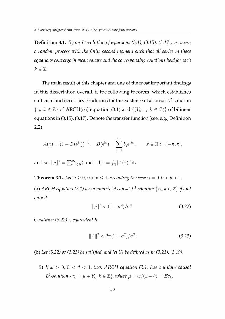
Definition 3.1. By an L2-solution of equations (3.1), (3.15), (3.17), we mean

a random process with the finite second moment such that all series in these

equations converge in mean square and the corresponding equations hold for each

k ∈ Z.

The main result of this chapter and one of the most important findings

in this dissertation overall, is the following theorem, which establishes

sufficient and necessary conditions for the existence of a causal L2-solution

τk, k ∈ Z of ARCH(∞) equation (3.1) and (Yk, zk, k ∈ Z) of bilinear

equations in (3.15), (3.17). Denote the transfer function (see, e.g., Definition

2.2)

A(x) = (1−B(eix))−1, B(eix) =∞∑j=1

bjeijx, x ∈ Π := [−π, π],

and set ‖g‖2 =∑∞

j=0 g2j and ‖A‖2 =

∫Π |A(x)|2dx.

Theorem 3.1. Let ω ≥ 0, 0 < θ ≤ 1, excluding the case ω = 0, 0 < θ < 1.

(a) ARCH equation (3.1) has a nontrivial causal L2-solution τk, k ∈ Z if and

only if

‖g‖2 < (1 + σ2)/σ2. (3.22)

Condition (3.22) is equivalent to

‖A‖2 < 2π(1 + σ2)/σ2. (3.23)

(b) Let (3.22) or (3.23) be satisfied, and let Yk be defined as in (3.21), (3.19).

(i) If ω > 0, 0 < θ < 1, then ARCH equation (3.1) has a unique causal

L2-solution τk = µ+ Yk, k ∈ Z, where µ = ω/(1− θ) = Eτk.

38

3.2. Stationary solutions of FIGARCH, IARCH and ARCH equations

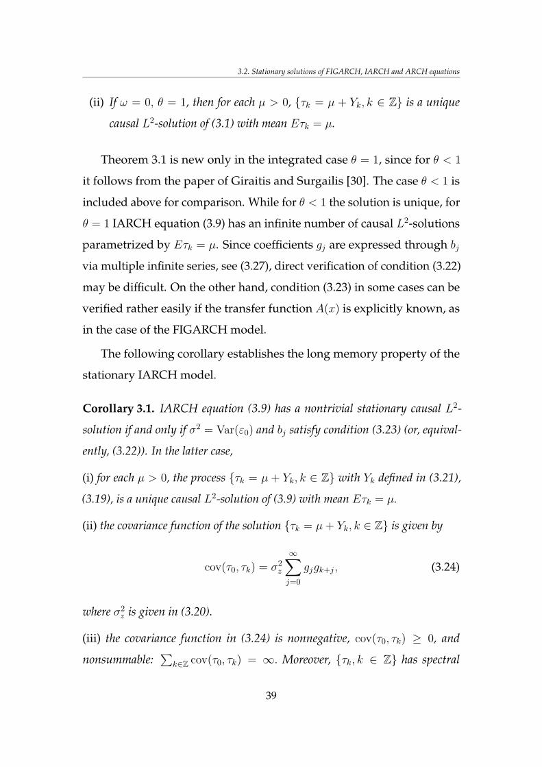
(ii) If ω = 0, θ = 1, then for each µ > 0, τk = µ + Yk, k ∈ Z is a unique

causal L2-solution of (3.1) with mean Eτk = µ.

Theorem 3.1 is new only in the integrated case θ = 1, since for θ < 1

it follows from the paper of Giraitis and Surgailis [30]. The case θ < 1 is

included above for comparison. While for θ < 1 the solution is unique, for

θ = 1 IARCH equation (3.9) has an infinite number of causal L2-solutions

parametrized by Eτk = µ. Since coefficients gj are expressed through bj

via multiple infinite series, see (3.27), direct verification of condition (3.22)

may be difficult. On the other hand, condition (3.23) in some cases can be

verified rather easily if the transfer function A(x) is explicitly known, as

in the case of the FIGARCH model.

The following corollary establishes the long memory property of the

stationary IARCH model.

Corollary 3.1. IARCH equation (3.9) has a nontrivial stationary causal L2-

solution if and only if σ2 = Var(ε0) and bj satisfy condition (3.23) (or, equival-

ently, (3.22)). In the latter case,

(i) for each µ > 0, the process τk = µ + Yk, k ∈ Z with Yk defined in (3.21),

(3.19), is a unique causal L2-solution of (3.9) with mean Eτk = µ.

(ii) the covariance function of the solution τk = µ+ Yk, k ∈ Z is given by

cov(τ0, τk) = σ2z

∞∑j=0

gjgk+j, (3.24)

where σ2z is given in (3.20).

(iii) the covariance function in (3.24) is nonnegative, cov(τ0, τk) ≥ 0, and

nonsummable:∑

k∈Z cov(τ0, τk) = ∞. Moreover, τk, k ∈ Z has spectral

39

3. Stationary integrated ARCH(∞) and AR(∞) processes with finite variance

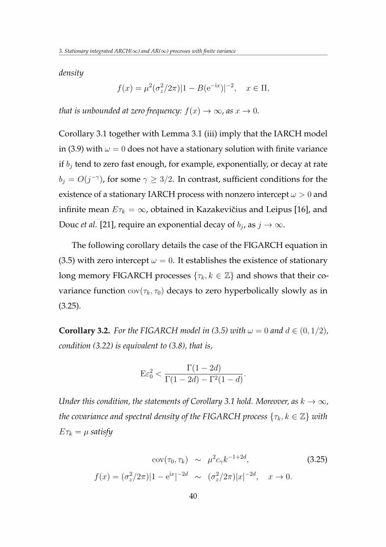
density

f(x) = µ2(σ2z/2π)|1−B(e−ix)|−2, x ∈ Π,

that is unbounded at zero frequency: f(x)→∞, as x→ 0.

Corollary 3.1 together with Lemma 3.1 (iii) imply that the IARCH model

in (3.9) with ω = 0 does not have a stationary solution with finite variance

if bj tend to zero fast enough, for example, exponentially, or decay at rate

bj = O(j−γ), for some γ ≥ 3/2. In contrast, sufficient conditions for the

existence of a stationary IARCH process with nonzero intercept ω > 0 and

infinite mean Eτk = ∞, obtained in Kazakevicius and Leipus [16], and

Douc et al. [21], require an exponential decay of bj , as j →∞.

The following corollary details the case of the FIGARCH equation in

(3.5) with zero intercept ω = 0. It establishes the existence of stationary

long memory FIGARCH processes τk, k ∈ Z and shows that their co-

variance function cov(τk, τ0) decays to zero hyperbolically slowly as in

(3.25).

Corollary 3.2. For the FIGARCH model in (3.5) with ω = 0 and d ∈ (0, 1/2),

condition (3.22) is equivalent to (3.8), that is,

Eε20 <

Γ(1− 2d)

Γ(1− 2d)− Γ2(1− d).

Under this condition, the statements of Corollary 3.1 hold. Moreover, as k →∞,

the covariance and spectral density of the FIGARCH process τk, k ∈ Z with

Eτk = µ satisfy

cov(τ0, τk) ∼ µ2cγk−1+2d, (3.25)

f(x) = (σ2z/2π)|1− eix|−2d ∼ (σ2

z/2π)|x|−2d, x→ 0.

40

3.2. Stationary solutions of FIGARCH, IARCH and ARCH equations

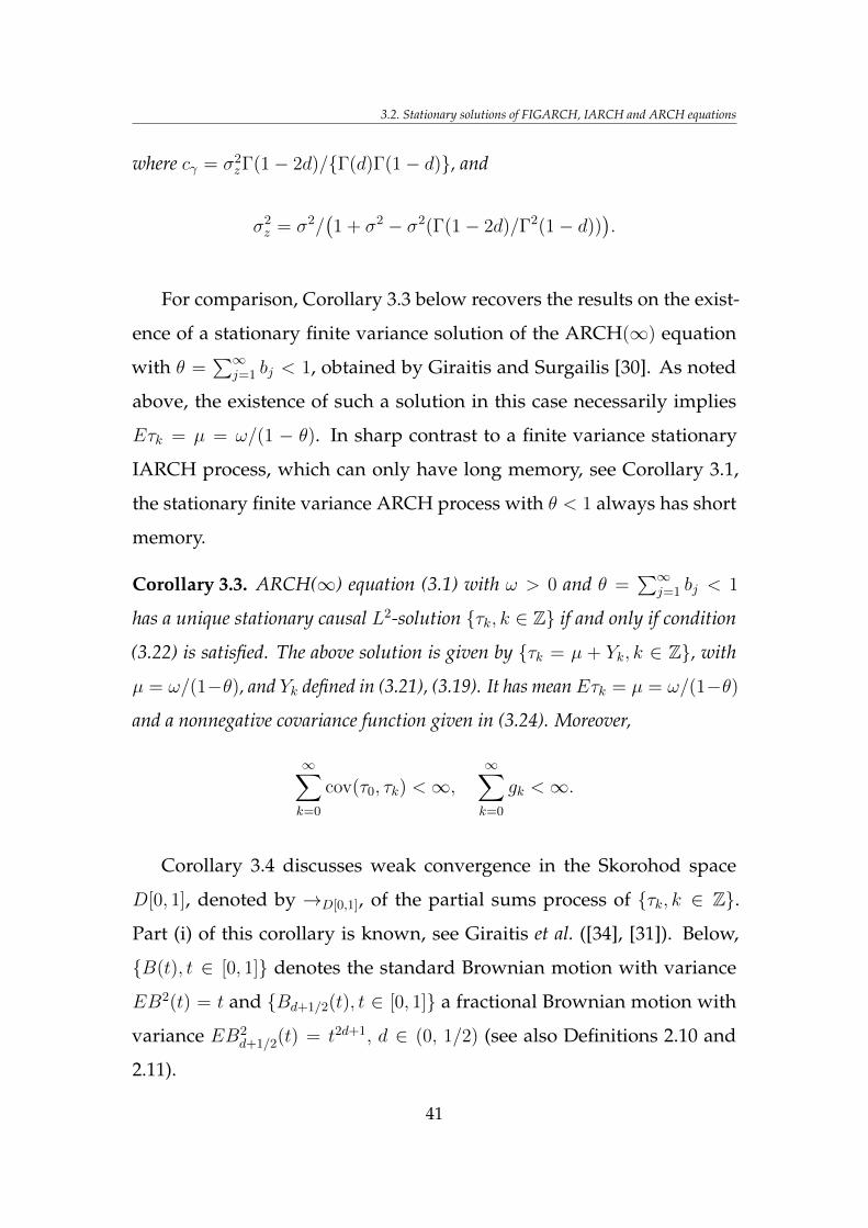
where cγ = σ2zΓ(1− 2d)/Γ(d)Γ(1− d), and

σ2z = σ2/

(1 + σ2 − σ2(Γ(1− 2d)/Γ2(1− d))

).

For comparison, Corollary 3.3 below recovers the results on the exist-

ence of a stationary finite variance solution of the ARCH(∞) equation

with θ =∑∞

j=1 bj < 1, obtained by Giraitis and Surgailis [30]. As noted

above, the existence of such a solution in this case necessarily implies

Eτk = µ = ω/(1 − θ). In sharp contrast to a finite variance stationary

IARCH process, which can only have long memory, see Corollary 3.1,

the stationary finite variance ARCH process with θ < 1 always has short

memory.

Corollary 3.3. ARCH(∞) equation (3.1) with ω > 0 and θ =∑∞

j=1 bj < 1

has a unique stationary causal L2-solution τk, k ∈ Z if and only if condition

(3.22) is satisfied. The above solution is given by τk = µ + Yk, k ∈ Z, with

µ = ω/(1−θ), and Yk defined in (3.21), (3.19). It has meanEτk = µ = ω/(1−θ)

and a nonnegative covariance function given in (3.24). Moreover,

∞∑k=0

cov(τ0, τk) <∞,∞∑k=0

gk <∞.

Corollary 3.4 discusses weak convergence in the Skorohod space

D[0, 1], denoted by →D[0,1], of the partial sums process of τk, k ∈ Z.

Part (i) of this corollary is known, see Giraitis et al. ([34], [31]). Below,

B(t), t ∈ [0, 1] denotes the standard Brownian motion with variance

EB2(t) = t and Bd+1/2(t), t ∈ [0, 1] a fractional Brownian motion with

variance EB2d+1/2(t) = t2d+1, d ∈ (0, 1/2) (see also Definitions 2.10 and

2.11).

41

3. Stationary integrated ARCH(∞) and AR(∞) processes with finite variance

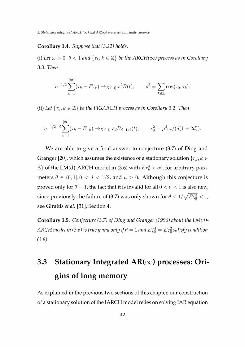
Corollary 3.4. Suppose that (3.22) holds.

(i) Let ω > 0, θ < 1 and τk, k ∈ Z be the ARCH(∞) process as in Corollary

3.3. Then

n−1/2

[nt]∑k=1

(τk − Eτk)→D[0,1] s2B(t), s2 =

∑k∈Z

cov(τ0, τk).

(ii) Let τk, k ∈ Z be the FIGARCH process as in Corollary 3.2. Then

n−1/2−d[nt]∑k=1

(τk − Eτk)→D[0,1] sdBd+1/2(t), s2d = µ2cγ/(d(1 + 2d)).

We are able to give a final answer to conjecture (3.7) of Ding and

Granger [20], which assumes the existence of a stationary solution rk, k ∈

Z of the LM(d)-ARCH model in (3.6) with Er4k <∞, for arbitrary para-

meters θ ∈ (0, 1], 0 < d < 1/2, and µ > 0. Although this conjecture is

proved only for θ = 1, the fact that it is invalid for all 0 < θ < 1 is also new,

since previously the failure of (3.7) was only shown for θ < 1/√Eζ4

0 < 1,

see Giraitis et al. [31], Section 4.

Corollary 3.5. Conjecture (3.7) of Ding and Granger (1996) about the LM(d)-

ARCH model in (3.6) is true if and only if θ = 1 andEζ40 = Eε2

0 satisfy condition

(3.8).

3.3 Stationary Integrated AR(∞) processes: Ori-

gins of long memory

As explained in the previous two sections of this chapter, our construction

of a stationary solution of the IARCH model relies on solving IAR equation

42

3.3. Stationary Integrated AR(∞) processes: Origins of long memory

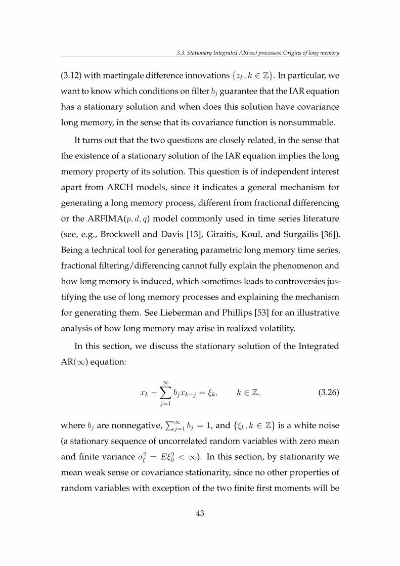
(3.12) with martingale difference innovations zk, k ∈ Z. In particular, we

want to know which conditions on filter bj guarantee that the IAR equation

has a stationary solution and when does this solution have covariance

long memory, in the sense that its covariance function is nonsummable.

It turns out that the two questions are closely related, in the sense that

the existence of a stationary solution of the IAR equation implies the long

memory property of its solution. This question is of independent interest

apart from ARCH models, since it indicates a general mechanism for

generating a long memory process, different from fractional differencing

or the ARFIMA(p, d, q) model commonly used in time series literature

(see, e.g., Brockwell and Davis [13], Giraitis, Koul, and Surgailis [36]).

Being a technical tool for generating parametric long memory time series,

fractional filtering/differencing cannot fully explain the phenomenon and

how long memory is induced, which sometimes leads to controversies jus-

tifying the use of long memory processes and explaining the mechanism

for generating them. See Lieberman and Phillips [53] for an illustrative

analysis of how long memory may arise in realized volatility.

In this section, we discuss the stationary solution of the Integrated

AR(∞) equation:

xk −∞∑j=1

bjxk−j = ξk, k ∈ Z, (3.26)

where bj are nonnegative,∑∞

j=1 bj = 1, and ξk, k ∈ Z is a white noise

(a stationary sequence of uncorrelated random variables with zero mean

and finite variance σ2ξ = Eξ2

0 < ∞). In this section, by stationarity we

mean weak sense or covariance stationarity, since no other properties of

random variables with exception of the two finite first moments will be

43

3. Stationary integrated ARCH(∞) and AR(∞) processes with finite variance

used.

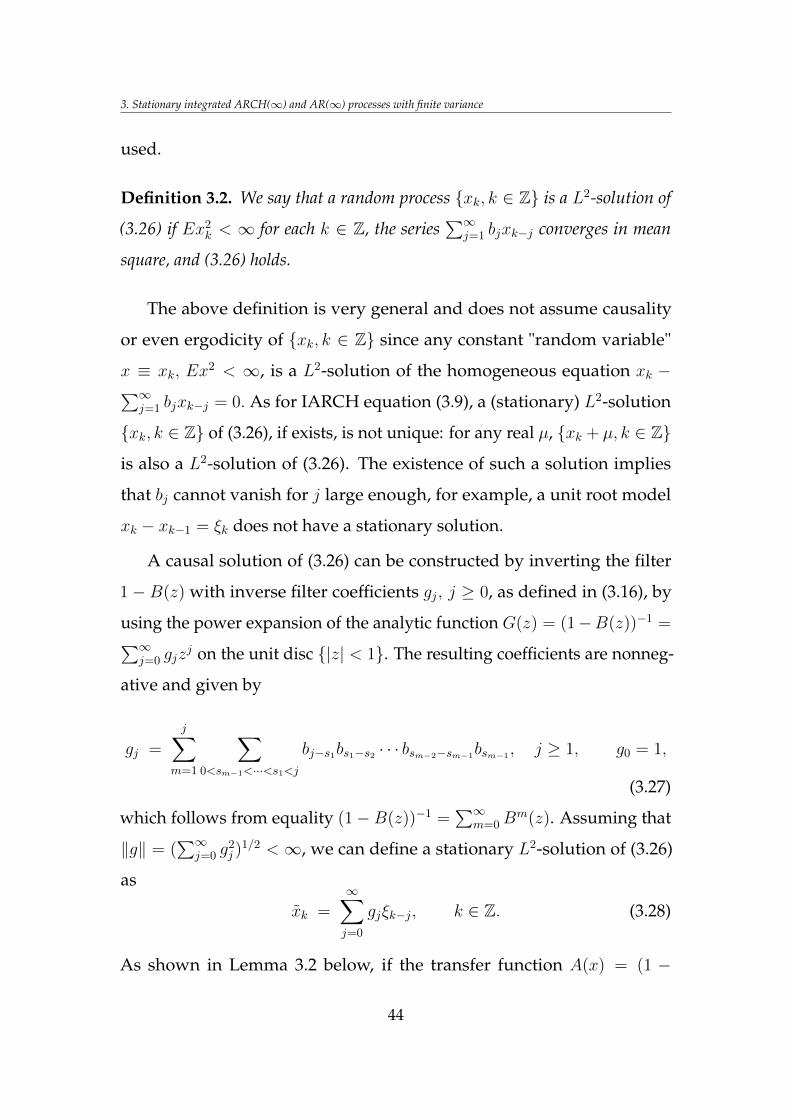
Definition 3.2. We say that a random process xk, k ∈ Z is a L2-solution of

(3.26) if Ex2k < ∞ for each k ∈ Z, the series

∑∞j=1 bjxk−j converges in mean

square, and (3.26) holds.

The above definition is very general and does not assume causality

or even ergodicity of xk, k ∈ Z since any constant "random variable"

x ≡ xk, Ex2 < ∞, is a L2-solution of the homogeneous equation xk −∑∞

j=1 bjxk−j = 0. As for IARCH equation (3.9), a (stationary) L2-solution

xk, k ∈ Z of (3.26), if exists, is not unique: for any real µ, xk + µ, k ∈ Z

is also a L2-solution of (3.26). The existence of such a solution implies

that bj cannot vanish for j large enough, for example, a unit root model

xk − xk−1 = ξk does not have a stationary solution.

A causal solution of (3.26) can be constructed by inverting the filter

1− B(z) with inverse filter coefficients gj, j ≥ 0, as defined in (3.16), by

using the power expansion of the analytic function G(z) = (1−B(z))−1 =∑∞j=0 gjz

j on the unit disc |z| < 1. The resulting coefficients are nonneg-

ative and given by

gj =

j∑m=1

∑0<sm−1<···<s1<j

bj−s1bs1−s2 · · · bsm−2−sm−1bsm−1, j ≥ 1, g0 = 1,

(3.27)

which follows from equality (1−B(z))−1 =∑∞

m=0Bm(z). Assuming that

‖g‖ = (∑∞

j=0 g2j )

1/2 < ∞, we can define a stationary L2-solution of (3.26)

as

xk =∞∑j=0

gjξk−j, k ∈ Z. (3.28)

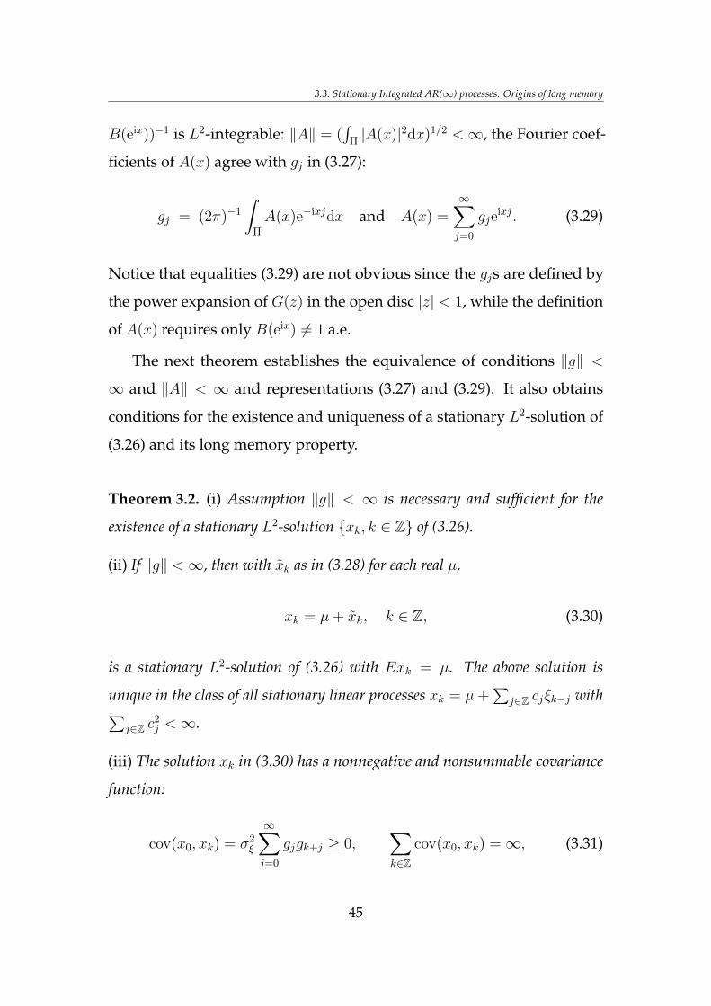
As shown in Lemma 3.2 below, if the transfer function A(x) = (1 −

44

3.3. Stationary Integrated AR(∞) processes: Origins of long memory

B(eix))−1 is L2-integrable: ‖A‖ = (∫

Π |A(x)|2dx)1/2 <∞, the Fourier coef-

ficients of A(x) agree with gj in (3.27):

gj = (2π)−1

∫Π

A(x)e−ixjdx and A(x) =∞∑j=0

gjeixj. (3.29)

Notice that equalities (3.29) are not obvious since the gjs are defined by

the power expansion of G(z) in the open disc |z| < 1, while the definition

of A(x) requires only B(eix) 6= 1 a.e.

The next theorem establishes the equivalence of conditions ‖g‖ <

∞ and ‖A‖ < ∞ and representations (3.27) and (3.29). It also obtains

conditions for the existence and uniqueness of a stationary L2-solution of

(3.26) and its long memory property.

Theorem 3.2. (i) Assumption ‖g‖ < ∞ is necessary and sufficient for the

existence of a stationary L2-solution xk, k ∈ Z of (3.26).

(ii) If ‖g‖ <∞, then with xk as in (3.28) for each real µ,

xk = µ+ xk, k ∈ Z, (3.30)

is a stationary L2-solution of (3.26) with Exk = µ. The above solution is

unique in the class of all stationary linear processes xk = µ+∑

j∈Z cjξk−j with∑j∈Z c

2j <∞.

(iii) The solution xk in (3.30) has a nonnegative and nonsummable covariance

function:

cov(x0, xk) = σ2ξ

∞∑j=0

gjgk+j ≥ 0,∑k∈Z

cov(x0, xk) =∞, (3.31)

45

3. Stationary integrated ARCH(∞) and AR(∞) processes with finite variance

and unbounded spectral density f(x) =σ2ξ

2π |1−B(eix)|−2 with limx→0 f(x) =∞.

(iv) ‖g‖ < ∞ implies ‖A‖ < ∞ and (3.29). Conversely, ‖A‖ < ∞ implies

‖g‖ <∞.

A surprising consequence of Theorem 3.2 is the fact that station-

ary solution (3.28) of (3.26) does not exist if the bjs vanish for j large

enough. The validity of this conclusion is not obvious from the rep-

resentation of gj in (3.27) but follows easily from (3.29). Indeed, since

|A(x)|−1 = |1 − B(eix)| = |∑∞

j=0 bj(1 − eijx)| ≤ |x|∑∞

j=1 j|bj| ≤ C|x|, this

implies∫

Π |A(x)|2dx ≥ C−2∫

Π x−2dx = ∞ and ‖g‖ = ∞ according to

(3.29). The above argument combined with Lemma 3.1 (iii) is formalized

in the following corollary.

Corollary 3.6. The IAR(∞) equation in (3.26) does not have a stationary L2-

solution if the bjs decay as j−3/2 or faster. In particular, the latter holds if

bj = 0, j > j0 for some j0 ≥ 1, or bj = O(e−cj) for j ≥ 1, c > 0.

The requirement of Theorem 3.2 that the r.h.s. ξk, k ∈ Z in IAR

equation (3.26) is white noise, is restrictive and can be relaxed. Theorem

3.3 extends Theorem 3.2 to the case when ξk, k ∈ Z is a short memory

process as precised below.

Theorem 3.3. Let ξk, k ∈ Z be a stationary process with zero mean, finite

variance and a spectral density fξ which is bounded away from 0 and∞:

c1 ≤ fξ(x) ≤ c2, ∀x ∈ Π, ∃ 0 < c1 < c2 <∞.

Then statements (i) and (ii) of Theorem 3.2 about a stationary solution of (3.26)

remain valid, while statement (iii) has to be modified as follows:

46

3.3. Stationary Integrated AR(∞) processes: Origins of long memory

(iii’) The solution xk, k ∈ Z in (3.30) has unbounded spectral density

f(x) = |1−B(eix)|−2fξ(x),

that satisfies limx→0 f(x) =∞, and a nonsummable autocovariance function:

∑k∈Z

|cov(x0, xk)| =∞.

Apparently, the class of stationary IAR(∞) processes with long memory

satisfying the conditions of Theorems 3.2 or 3.3 is quite large. Since condi-

tion θ =∑∞

j=1 bj = 1 does not assume any particular form of bj , it seems

that the spectral density of an IAR(∞) process need not grow regularly as

a power function |x|−α, 0 < α < 1, at x = 0 and, similarly, the covariance

function need not decay regularly with the lag as k−1+α. The latter proper-

ties are key features of fractionally integrated ARFIMA models (see, e.g.,

Hosking [44], also Giraitis et al. [36], Chapter 7).

Example 3.1. The ARFIMA(0, d, 0) model is defined as a stationary solu-

tion of the equation

(1− L)dxk = ξk, 0 < d < 1/2,

where ξk, k ∈ Z is uncorrelated white noise with Eξk = 0, Eξ2k = σ2

ξ .

It can be written as the IAR(∞) equation in (3.26) with bj generated

by B(z) = 1 − (1 − z)d =∑∞

j=1 bjzj . The transfer function A(x) =

(1 − B(e−ix))−1 satisfies |A(x)| = |1 − e−ix|−2d ∼ |x|−2d, as x → 0, and

is integrable for d ∈ (0, 1/2). The coefficients bj and gj of the generating

47

3. Stationary integrated ARCH(∞) and AR(∞) processes with finite variance

functions B(z) and G(z) = (1−B(z))−1 = (1− z)−d are given by

bj = − Γ(j − d)

Γ(j + 1)Γ(−d), gj =

Γ(j + d)

Γ(j + 1)Γ(d), j ≥ 1, g0 = 1. (3.32)

They have properties bj > 0, gj > 0, θ =∑∞

j=1 bj = 1, and

bj ∼ −j−d−1/Γ(−d), gj ∼ jd−1/Γ(−d), j →∞, (3.33)

so that ‖g‖ <∞. Relations (3.33) imply that the covariance

γk = cov(x0, xk) = σ2ξ

∞∑j=0

gjgk+j

decays hyperbolically, that is,

γk ∼ cγk−1+2d, cγ =

σ2ξΓ(1− 2d)

Γ(d)Γ(1− d), (3.34)

and the spectral density is singular at the origin:

f(x) = (σ2ξ/2π)|1− eix|−2d ∼ cf |x|−2d, cf = σ2

ξ/2π.

Example 3.2. A nonparametric (depending on an infinite number of para-

meters) class of IAR processes xk =∑∞

j=1 bjxk−j + ξk generalizing the

previous example is defined by equation (3.26) with uncorrelated noise

ξk, k ∈ Z and coefficients bj generated by the operator

B(L) =(1− (1− L)d

)P (L) =

∞∑j=1

bjLj, 0 < d < 1/2. (3.35)

Here, P (z) =∑∞

j=0 pjzj is a generating function with coefficients satisfy-

48

3.3. Stationary Integrated AR(∞) processes: Origins of long memory

ing

pj ≥ 0, p0 > 0,∞∑j=0

pj = 1 and∞∑j=1

jpj <∞. (3.36)

Then bj =∑j−1

k=0 pkb0j−k, where b0

j are the coefficients of the expansion

1− (1− z)d =∑∞

j=1 b0jzj , see (3.32). Hence, the bj in (3.35) are nonnegative

and sum up to 1.

Let us show that |A(x)|2 = |1−B(eix)|−2 is integrable. Since b1 = p0b01 >

0, by Lemma 3.1 (ii) |A(x)| is bounded on [ε, π] for any ε > 0. Therefore,

it suffices to show that |A(x)|2 is integrable at x = 0. To this end, rewrite

1−B(eix) = 1−(1− (1− eix)d

)P (eix) = (1− eix)dh(x), where

h(x) = P (eix)−(P (eix)− 1

)(1− eix)−d. (3.37)

From (3.36) we have |P (eix) − 1| =∑∞

j=1 |eijx − 1|pj ≤ |x|∑∞

j=1 jpj =

O(|x|) = o(|(1 − eix)d|) and, therefore, limx→0 h(x) = h(0) = P (1) = 1.

Hence, |A(x)|2 ∼ |x|−2d, x → 0, proving the integrability of |A(x)|2 for

d ∈ (0, 1/2). The corresponding stationary solution xk, k ∈ Z of (3.26)

with uncorrelated noise ξk has spectral density

f(x) = (σ2ξ/2π)|1−B(e−ix)|−2 = (σ2

ξ/2π)|1− e−ix|−2d|h(x)|−2, x ∈ Π,

(3.38)

with h defined at (3.37). It satisfies f(x) ∼ (σ2ξ/2π)|x|−2d, x → 0, and

is a continuous bounded function on intervals [ε, π], ε > 0. Moreover,

using (3.38), (3.37), (3.36) and Lemma 2.3.1 of Giraitis et al. [36], one can

show that the asymptotics of the covariance function is cov(x0, xk) ∼

cγk−1+2d, k →∞, with cγ given in (3.34) is the same as for ARFIMA(0, d, 0)

model. Hence, the pj or P (L) in (3.35) essentially affects short memory

dynamics and do not affect the long-run behavior of the corresponding

49

3. Stationary integrated ARCH(∞) and AR(∞) processes with finite variance

IAR process.

Example 3.3. (The IAR(q, d) model). We introduce the parametric class

IAR(q, d) consisting of IAR(∞) processes (3.26) with B(L) as in (3.35)

and P (L) a polynomial of degree q satisfying (3.36). It is convenient to

parameterize such polynomials as

P (z) =1 + r1z + · · ·+ rqz

q

1 + r1 + · · ·+ rq, r1 ≥ 0, . . . , rq ≥ 0.

Thus, pi = ri/(1 + · · · + rq), 1 ≤ i ≤ q, p0 = 1/(1 + · · · + rq), satisfy (3.36)

so that IAR(q, d) is a particular case and shares the same long memory

properties as IAR in Example 3.2. Note that the IAR(0, d) model coincides

with ARFIMA(0, d, 0). Apart from this case, it seems that the IAR(q, d)

models are different from the ARFIMA(p, d, q) models. For example, the

model (1−B(L))xk = ξk with B(z) = (1− (1− z)d)(1 + rz)/(1 + r) with

P (z) = (1 + rz)/(1 + r) generates a different covariance structure than the

ARFIMA(1, d, 0) model (1− L)d(1 + rL)xk = ξk.

3.4 Proofs of Theorem 3.1 and Corollaries 3.1-

3.4

The following proposition used to prove Theorem 3.1 establishes the

relation between solutions τk of ARCH(∞) equation (3.1), and (Yk, zk) of

bilinear equations (3.15) and (3.17), with εk and ζk related by εk = σζk + 1,

and ω = µ(1 − θ). For Yk in (3.15), we define "noise" as zk = ζk(µσ +

σ∑∞

j=1 bjYk−j). For zk in (3.17), the volatility process vk is defined in

(3.18).

50

3.4. Proofs of Theorem 3.1 and Corollaries 3.1-3.4

Proposition 3.1. Let 0 < µ <∞ and θ ∈ (0, 1].

(i) If τk, k ∈ Z is a causal L2-solution of (3.1), then Yk = τk − µ, k ∈ Z is a

causal L2-solution of (3.15) such that Yk ≥ −µ.

(ii) If Yk, k ∈ Z is a causal L2-solution of (3.15) such that Yk ≥ −µ, then

τk = Yk + µ, k ∈ Z is a causal L2-solution of equation (3.1).

(iii) Yk, k ∈ Z is a causal L2-solution of bilinear equation (3.15) if and only if

Yk, zk, k ∈ Z is a causal L2-solution of equation (3.17). Moreover, Yk ≥ −µ

is equivalent to vk ≥ 0 with vk as in (3.18).

Proof. The equivalence of (i) and (ii) is immediate. We only need to

prove (iii). Let Yk, k ∈ Z be a causal L2-solution of (3.15). Set zk =

ζk(µσ + σ∑∞

j=1 bjYk−j) and denote vk = µσ +∑∞

j=1 hjzk−j . Let us prove

that Yk, zk, k ∈ Z is a causal L2-solution of (3.17). This follows from

(3.15) and equality

vk = µσ + σ∞∑j=1

bjYk−j, (3.39)

which is verified below. From the definition of zk and (3.15) it follows

that Yk satisfy the IAR equation Yk −∑∞

j=1 bjYt−j = zk, where zk, k ∈ Z

is a causal uncorrelated process with finite variance. Therefore, by The-

orem 3.2 we have Yk =∑∞

j=0 gjzk−j , which implies that σ∑∞

j=1 bjYk−j =

σ∑∞

j=1 bj∑∞

i=0 gizk−j−i =∑∞

j=1 hjzk−j in view of the definition of hj in

(3.16), proving (3.39) and the fact that Yk, zk is a causal L2-solution

of (3.17). Moreover, Yk−j ≥ −µ, k ∈ Z, and (3.39) imply vk ≥ µσ +

σ(∑∞

j=1 bj)(−µ) = µσ(1− θ) ≥ 0, k ∈ Z.

Conversely, assume that Yk, zk, k ∈ Z is a causal L2-solution of (3.17).

Then the claim that Yk, k ∈ Z is a causal L2-solution of (3.15) follows

from (3.39), which, in turn, follows from Theorem 3.2 using exactly the

51

3. Stationary integrated ARCH(∞) and AR(∞) processes with finite variance

same argument as above. Finally, from vk ≥ 0, (3.39), (3.15) and ζk ≥ −1/σ,

we obtain

Yk =∞∑j=0

bjYk−j + ζkvk ≥∞∑j=0

bjYk−j − (1/σ)vk

=∞∑j=0

bjYk−j − (1/σ)(µσ + σ

∞∑j=0

bjYk−j) = −µ,

proving part (iii) and the proposition.

Proof of Theorem 3.1. (a) The equivalence of (3.22) and (3.23) follows

from the equivalence of ‖g‖ < ∞ and ‖A‖ < ∞, see Lemma 3.2, and

Parseval’s identity ‖g‖ = 2π‖A‖. Let us prove the necessity of condition

(3.22), or ‖h‖ < 1, for the existence of a stationary solution. Assume

that τk, k ∈ Z is an L2-solution of ARCH equation (3.1). Then, by

Proposition 3.1 (i), the last fact implies that for µ > 0,Yk = τk − µ, zk =

ζk(µσ+σ∑∞

j=1 bjYk−j), k ∈ Z

is an L2-solution of bilinear equation (3.17).

Consequently, σ2z = Ez2

k = E(µσ+

∑∞j=1 hjzk−j

)2= (µσ)2 +(

∑∞j=1 h

2j)σ

2z =

(µσ)2 + ‖h‖2σ2z , yielding ‖h‖2 < 1, or (3.22), since ‖h‖2 = σ2(‖g‖2 − 1).

Conversely, let us show that ‖h‖ < 1 implies the existence of the L2-

solution τk, k ∈ Z of (3.1) with Eτk = µ given by τk = Yk + µ and Yk

defined in (3.21), (3.19). As shown in (3.20), ‖h‖ < 1 guarantees that Yk

is an L2-solution of (3.15). Therefore, by Proposition 3.1 (ii), it suffices to

prove that

Yk ≥ −µ. (3.40)

To show (3.40), we approximate Yk by

Yk,p = (µσ)∞∑m=1

∑p<sm<···<s1≤k

gk−s1hs1−s2 · · ·hsm−1−smζs1 · · · ζsm

,

52

3.4. Proofs of Theorem 3.1 and Corollaries 3.1-3.4

where −p ≥ 1 is a large integer. Observe that for k > p the Yk,p satisfy

equation (3.15), viz.,

Yk,p = ζk

(µσ + σ

∞∑j=1

bjYk−j,p

)+∞∑j=1

bjYk−j,p, for k > p, (3.41)

while Yk,p = 0 for k ≤ p. Moreover, by orthogonality of Volterra series,

E(Yk − Yk,p)2 = (µσ)2∑∞

m=1 J(m)k,p , where

J(m)k,p =

∑sm<···<s1≤k, sm≤p

g2k−s1h

2s1−s2 · · ·h

2sm−1−sm.

Notice that J (m)k,p ≤ ‖g‖2‖h‖2(m−1), where ‖h‖ < 1. Hence,

∑∞m=1 J

(m)k,p is

dominated by a converging series. Moreover, for each m ≥ 1, J (m)k,p → 0

as p → −∞. Hence, limp→−∞E(Yk − Yk,p)2 = 0 for any k ∈ Z by the

dominated convergence theorem. Therefore, (3.40) follows if we show

that for any p ∈ Z,

Yk,p ≥ −µ, k ∈ Z. (3.42)

To prove (3.42), we use induction on k. Clearly, (3.42) holds for k ≤ p

because by definition Yk,p = 0 > −µ for k ≤ p. Also, (3.42) holds for k =

p+ 1, since Yp+1,p = (µσ)ζp+1 ≥ −µ because (µσ)ζj = (µσ)(εj−1)/σ ≥ −µ,

for j ∈ Z. Let k > p+ 1. Assume by induction that Ys,p ≥ −µ for all s < k.

Then, by (3.41) and the inductive assumption,

Yk,p = ζk(µσ) + (ζkσ + 1)

( ∞∑j=1

bjYk−j,p

)≥

≥ ζk(µσ) + (ζkσ + 1)

( ∞∑j=1

bj

)(−µ) = −µ.

53

3. Stationary integrated ARCH(∞) and AR(∞) processes with finite variance

This proves the induction step k − 1 → k as well as (3.42) and (3.40),

thereby proving part (a) of the theorem.

(b) Claim (i) is shown in Giraitis et al. [30], Theorem 3.1. Let us prove (ii).

By part (a), it suffices to prove the uniqueness of the solution τk, k ∈ Z.

Let τ ′k, k ∈ Z, τ ′′k , k ∈ Z be two causal L2-solutions of (3.1) with Eτ ′k =

Eτ ′′k . Then τ ′k − τ ′′k = Yk is a causal L2-solution of Yk =∑∞

j=1 bjYk−j + zk,

where zk = ζkσ∑∞

j=1 bjYk−j . By causality, the stationary process Yk =

f(εk, εk−1, . . . ) is a function of lagged i.i.d. variables. Hence, Yk is a

regular process withEY 2k <∞, having spectral density, see Ibragimov and

Linnik [48], Theorem 17.1.2. Moreover, zk = ζk∑∞

j=1 hjzk−j , see (3.17) (b),

where zk, k ∈ Z is covariance stationary white noise and∑∞

j=1 h2j =

‖h‖2 < 1, Eζ2k = 1. Then Ez2

k =∑∞

j=1 h2jEz

2k−j = ‖h‖2Ez2

k implies Ez2k = 0

and hence zk = 0. Therefore, Yk, k ∈ Z has spectral density and is a

stationary solution of the homogeneous equation Yk −∑∞

j=1 bjYk−j = 0.

As shown in the proof of Theorem 3.2 (ii) below, such an equation has a

unique solution Yk ≡ 0, proving the uniqueness of τk, k ∈ Z. Theorem

3.1 is proved.

Proof of Corollary 3.1. All claims with the exception of (iii) follow from

Theorem 3.1, and claim (iii) follows from Theorem 3.2 (iii).

Proof of Corollary 3.2. Note σ2 = Eε20 − 1. We have ‖A‖2 =

∫Π |1 −

eix|−2ddx = 2πΓ(1− 2d)/Γ2(1− d) yielding the equivalence of (3.23) and

(3.8). The remaining claims follow from Corollary 3.1 and fact (3.34) in

Example 3.1.

Proof of Corollary 3.3. All statements with the exception of the last claim

follow from Theorem 3.1. To show it, note that gj ≥ 0 in (3.27) satisfy∑∞j=0 gj ≤

∑∞m=0 θ

m <∞ since θ < 1.

54

3.5. Proofs of Theorems 3.2 and 3.3

Proof of Corollary 3.4. It suffices to only show part (ii). Using the fact

that by (3.21) Yk = τk − Eτk =∑∞

j=0 gjzk−j is a moving average in sta-

tionary ergodic martingale differences zs of (3.19) with coefficients gj

given in (3.32) and satisfying (3.33), the convergence in (ii) follows from

Theorem 3.1 in Abadir et al. [1] or Theorem 6.2 in Giraitis and Surgailis

[30].

Proof of Corollary 3.5. Let θ = 1. Then the LM(d)-ARCH model in (3.6)

coincides with the FIGARCH model in (3.5) with ω = 0 and the statement

follows from Corollary 3.2. Next, let θ < 1. Then (3.6) can be written

as the ARCH(∞) equation in (3.1) with ω = µ(1 − θ) > 0. According

to Corollary 3.3, the squared process r2k = τk has short memory and

summable autocovariance∑∞

k=0 cov(r20, r

2k) < ∞ which contradicts (3.7).

3.5 Proofs of Theorems 3.2 and 3.3

The proof of Theorem 3.1 uses auxiliary Lemmas 3.1 and 3.2. The proofs

of these lemmas are provided at the end of this section. Denote Jb =

j ≥ 1 : bj > 0, and assume Jb has at least two elements. Denote by

gcd(Jb) the greatest common divisor of j ∈ Jb. For example, if b1 > 0, then

gcd(Jb) = 1, and if b2j > 0, b2j−1 = 0, j = 1, 2, . . . , then gcd(Jb) = 2.

Lemma 3.1. Let θ =∑∞

j=1 bj = 1.

(i) The function 1 − B(eix), x ∈ Π, has only finite number of zeroes on Π,

including x = 0.

(ii) The point x = 0 is the unique zero of 1−B(eix) if and only if gcd(Jb) = 1.

(iii) If bk = O(k−γ), k →∞, for some γ ≥ 3/2, then ‖A‖ =∞.

55

3. Stationary integrated ARCH(∞) and AR(∞) processes with finite variance

Lemma 3.2. Let θ ≤ 1.

(i) If ‖g‖ <∞ then ‖A‖ <∞ and (3.29) hold.

(ii) If ‖A‖ <∞ then ‖g‖ <∞.

Proof of Theorem 3.2. All statements in (iv) follow from Lemma 3.2.

(i) If ‖g‖ < ∞, then by (iv), ‖A‖ < ∞ and (3.29) holds. Evidently, this

implies that (3.28) is a stationary solution of (3.26).

Conversely, if a stationary solution xk, k ∈ Z of (3.26) exists, it

suffices to prove that ‖A‖ < ∞, which by (iv) implies ‖g‖ < ∞. Let

xk =∫

Π eikyZx(dy) be the spectral representation of xk, k ∈ Z and

Fx(dy) = E|Zx(dy)|2 be its spectral measure (we do not assume a priori that

xk, k ∈ Z has spectral density). Denote by ξk =∫

Π eikyZξ(dy) the spectral

representation of the noise ξk, k ∈ Z and by Fξ(dy) = E|Zξ(dy)|2 =

(σ2ξ/2π)dy its spectral measure. Since the series B(eiy) =

∑∞j=1 bje

ijy

converges uniformly in Π to a bounded function, xk −∑∞

j=1 bjxk−j =∫Π(1−B(eiy))Zx(dy) = ξk =

∫Π eikyZξ(dy), leading to

|1−B(eiy)|2Fx(dy) = Fξ(dy) = (σ2ξ/2π)dy, y ∈ Π. (3.43)

By Lemma 3.1 (i), 1 − B(e−iy) has a finite number of zeros y1, . . . , ym ∈

Π. Since Fx is nondecreasing, (3.43) implies that Fx(dy) coincides with

f(y)dy, f(y) = (σ2ξ/2π)|A(y)|2, except for possible jumps at points y1, . . . ,

ym, i.e. Fx(dy) = f(y)dy +∑m

i=1 ciδyi, where ci ≥ 0 are some nonnegative

constants. Therefore,

∞ > Ex2k =

∫Π

Fx(dy) ≥∫

Π

f(y)dy = (σ2ξ/2π)

∫Π

|A(y)|2dy,

proving ‖A‖ <∞.

56

3.5. Proofs of Theorems 3.2 and 3.3

(ii) Since xk, k ∈ Z in (3.28) is a zero mean L2-solution of equation (3.26),

see the proof of (i) above, it remains to show the uniqueness of solution

xk = µ + xk of (3.26) with the stated properties. Let x′k, k ∈ Z, x′′k, k ∈

Z, be two stationary L2-solutions of (3.26) with Ex′k = Ex′′k and let

yk = x′k − x′′k. Moreover, by the assumption in (ii), yk has the form yk =∑j∈Z cjξk−j with

∑j∈Z c

2j <∞. The above facts imply that yk, k ∈ Z is

a L2-solution of the homogeneous equation yk −∑∞

j=1 bjyk−j = 0 and a

stationary process with absolutely continuous spectral measure Fy(dx) =

fy(x)dx, fy(x) = (σ2ξ/2π)|

∑j∈Z cje

ijx|2 and a spectral representation yk =∫Π eikxZy(dx). Since

∑∞j=1 eijxbj converges uniformly on Π, hence also in

L2(Fy), it follows that yk −∑∞

j=1 bjyk−j =∫

Π(1 − B(eix))Zy(dx) = 0 and∫Π |1−B(eix)|2Fy(dx) = 0. Together with Lemma 3.1 (i), this implies that

fy(x) = 0 a.e. on Π and hence Fy = 0 and yk = 0, proving part (ii).

(iii) As noted above, solution xk in (3.28) has spectral density f(x) =

(σ2ξ/2π)|1 − B(eix)|−2. Relation limx→0 f(x) = ∞ follows from B(1) = 1,

continuity of B(e−ix), and the fact |B(x)| < 1 for 0 < x < x0 for some x0 >

0 which holds by Lemma 3.1 (i). The divergence∑

k∈Z |cov(x0, xk)| =∞

is immediate from the previous fact. Finally, the first claim in (3.31) is a

consequence of moving average representation (3.28) and positivity of gj .

Theorem 3.2 is proved.

Proof of Theorem 3.3. The proof follows using the same arguments as in

the proof of Theorem 3.2.

Proof of Lemma 3.1. (i) First observe that B(eix) = θ = 1 holds for

x = 0. Suppose that x ∈ (0, 2π) is such that 1 = B(eix). Then B(eix) is

a real number: B(eix) =∑∞

j=1 bj cos(jx) and then 1 =∑∞

j=1 bj cos(jx) ≤

57

3. Stationary integrated ARCH(∞) and AR(∞) processes with finite variance

∑∞j=1 bj = 1 is possible if and only if 1 = cos(jx) = eijx for all j ∈ Jb, or

x/2π ∈⋂j∈Jb

Ij, where Ij =

1

j,2

j, . . . ,

j − 1

j

. (3.44)

Clearly, since each Ij is a finite set, the intersection in (3.44) is a finite set

as well, proving (i).

(ii) Let gcd(Jb) = 1. Then gcd(j1, j2) = 1 for j1, j2 ∈ Jb, j1 6= j2. It suffices

to show that Ij1 ∩ Ij2 = ∅. Indeed, assume ad absurdum that Ij1 ∩ Ij2 6= ∅,

then k2 = k1j2/j1 for some integers 1 ≤ k1 < j1, 1 ≤ k2 < j2, by definition

of Ij in (3.44). Since j1 and j2 are coprimes, this means that j1 is a divisor

of k1, or k1 ∈ j1, 2j1, . . . , which contradicts k1 < j1.

Let p = gcd(Jb) ≥ 2. Then for any j ∈ Jb, j = j′p with 1 ≤ j′ < j. Thus,

j/p ∈ 1, 2, . . . , j − 1, implying 1/p ∈ Ij for all j ∈ Jb and 1/p ∈⋂j∈Jb Ij .

Particularly, x = 2π/p 6= 0 is a zero of 1−B(eix).

(iii) It suffices to show |1 − B(eix)| ≤ C|x|1/2 as this implies∫

Π |1 −

B(eix)|−2dx ≥ C−1∫

Π dx/|x| = ∞. We have |1 − eijx| ≤ min(j|x|, 2), bj ≤

Cj−γ ≤ Cj−3/2 and thus

∣∣1−B(eix)∣∣ =

∣∣∣ ∞∑j=1

bj(1− eijx)∣∣∣ ≤ C|x|

∑1≤j<1/|x|

j1/2 +

+ C∑

j≥1/|x|

j−3/2 ≤ C|x|1/2.

This proves (iii) and the lemma, too.

Proof of Lemma 3.2. (i) Suppose that ‖g‖ <∞. Set kr(x) =∑∞

j=0 gjrjeijx,

58

3.5. Proofs of Theorems 3.2 and 3.3

0 < r < 1. Then kr is a Cauchy sequence in L2(Π):

‖kr − kr′‖2 =

∫Π

∣∣∣ ∞∑j=0

gj(rj − r′ j)eijx

∣∣∣2dx = 2π∞∑j=0

g2j |rj − r′ j|2 → 0,

as r, r′ ↑ 1. Moreover, kr(x) → A(x) = (1 − B(eix))−1 a.e. in Π as r ↑ 1,

since kr(x) = G(reix) = (1−B(reix))−1 for 0 < r < 1 and 1−B(eix) 6= 0 a.e.

in Π (see Lemma 3.1 (i)). Therefore, ‖kr − A‖ → 0 as r ↑ 1 and ‖A‖ <∞,

see Rudin ([65], Thorem 3.12). Since k1 ∈ L2(Π) and ‖kr − k1‖2 → 0 as

r ↑ 1, then A = k1 in L2(Π) which proves (3.29).

(ii) Let ‖A‖ <∞. Then functions hk(x) = e−ikx/(1−B(eikx)) = e−ikxA(x),

x ∈ Π, k ∈ Z belong to the Hilbert space L2(Π) with the norm

‖h‖ =

(∫Π

|h(x)|2dx

)1/2

.

So, ‖hk‖ = ‖A‖ <∞. Then hk(x)−∑∞

j=1 bjhk−j(x) = eikx, where the series

converges in L2(Π). By Lemma 3.1 (iii), ‖A‖ < ∞ implies that bj > 0

for infinite number of j. For a large p ≥ 1 denote b′j = bjI(j ≤ p) and

B′(eix) =∑∞

j=1 b′je

ijx. Then

hk(x)−p∑j=1

bjhk−j(x) = eikx + uk(x), where uk(x) =∞∑

j=p+1

bjhk−j(x).

Since∑p

j=1 bjhk−j(x) = hk(x)B′(eix) and∑p

j=1 bj =∑∞

j=1 b′j < 1, we obtain

hk(x) =eikx + uk(x)

1−B′(eix)= ξ′k(x) + u′k(x),

where

ξ′k(x) =eikx

1−B′(eix), u′k(x) =

uk(x)

1−B′(eix).

59

3. Stationary integrated ARCH(∞) and AR(∞) processes with finite variance

We claim that under assumption ‖g‖ =∞, as p→∞,

‖u′k‖ ≤ ‖hk‖ = ||A|| <∞ and ‖ξ′k‖ → ∞. (3.45)

On the other hand, ‖ξ′k‖ = ‖hk − u′k‖ ≤ ‖hk‖ + ‖u′k‖ ≤ 2‖hk‖ < C < ∞,

which leads to a contradiction, implying ‖g‖ <∞.

To prove (3.45), note that from the definition of u′k(x) and

1 ≤∣∣∣1− p∑

j=1

bje−ijx∣∣∣+∣∣∣ p∑j=1

bje−ijx∣∣∣ ≤ ∣∣∣1− p∑

j=1

bje−ijx∣∣∣+

p∑j=1

bj

we obtain

‖u′k‖2 =

∫Π

∣∣∣ ∑∞j=p+1 bje

−ijx

(1−B(eix))(1−∑p

j=1 bje−ijx)

∣∣∣2dx

≤∫

Π

dx

|1−B(eix)|2

( ∑∞j=p+1 bj

1−∑p

j=1 bj

)2

≤∫

Π

dx

|1−B(eix)|2= ‖hk‖2,

proving the first relation in (3.45). The second claim in (3.45) follows from

‖ξ′k‖2 =

∫Π

dx

|1−B′(eix)|2=

∫Π

|G′(eix)|2dx = 2π∞∑j=0

(g′j)2,

where g′j are power coefficients of the analytic function G′(z) = (1 −

B′(z))−1 =∑∞

j=0 g′jzj, |z| < 1, as given by (3.27) with bj replaced by b′j .

Note 0 ≤ g′j → gj monotonically as p → ∞ and, therefore,∑∞

j=0(g′j)2 →

‖g‖2 =∞. This proves part (ii) and completes the proof of the lemma.

60

3.6. Simulation study

3.6 Simulation study

This section consists of two parts. In the first one, we simulate and

compare FIGARCH and ARFIMA(0, d, 0) processes and their estimated

autocorrelation functions. The second part is devoted to the investigation

of similarities and differences between IAR(p, d, q) and ARFIMA(p, d, q)

models.

3.6.1 FIGARCH and ARFIMA(0,d,0) processes

First we describe the simulation procedure. We generate N = 500 samples

of length n = 20000 each, with the first np = 10000 values being the

pre-sample which is not used in the subsequent calculations of autocorrel-

ations. The FIGARCH process was generated using equation

τk = εk

(np−1+k∑j=1

bjτk−j + 1−np−1+k∑j=1

bj

), −np + 1 ≤ k ≤ np, (3.46)

and the ARFIMA(0, d, 0) process comes from equation

xk = ζk +

np−1+k∑j=1

bjxk−j +

(1−

np−1+k∑j=1

bj

), −np + 1 ≤ k ≤ np. (3.47)

Initial conditions for both processes are τk = xk = 1, k ≤ 0, and coefficients

bj are determined by the generating function B(z) =∑∞

j=1 bjzj = 1− (1−

z)d. We calculate them using the recursive relation

b1 = d,

bj = bj−1d− j + 1

j(−1)2j+1, j ≥ 2.

61

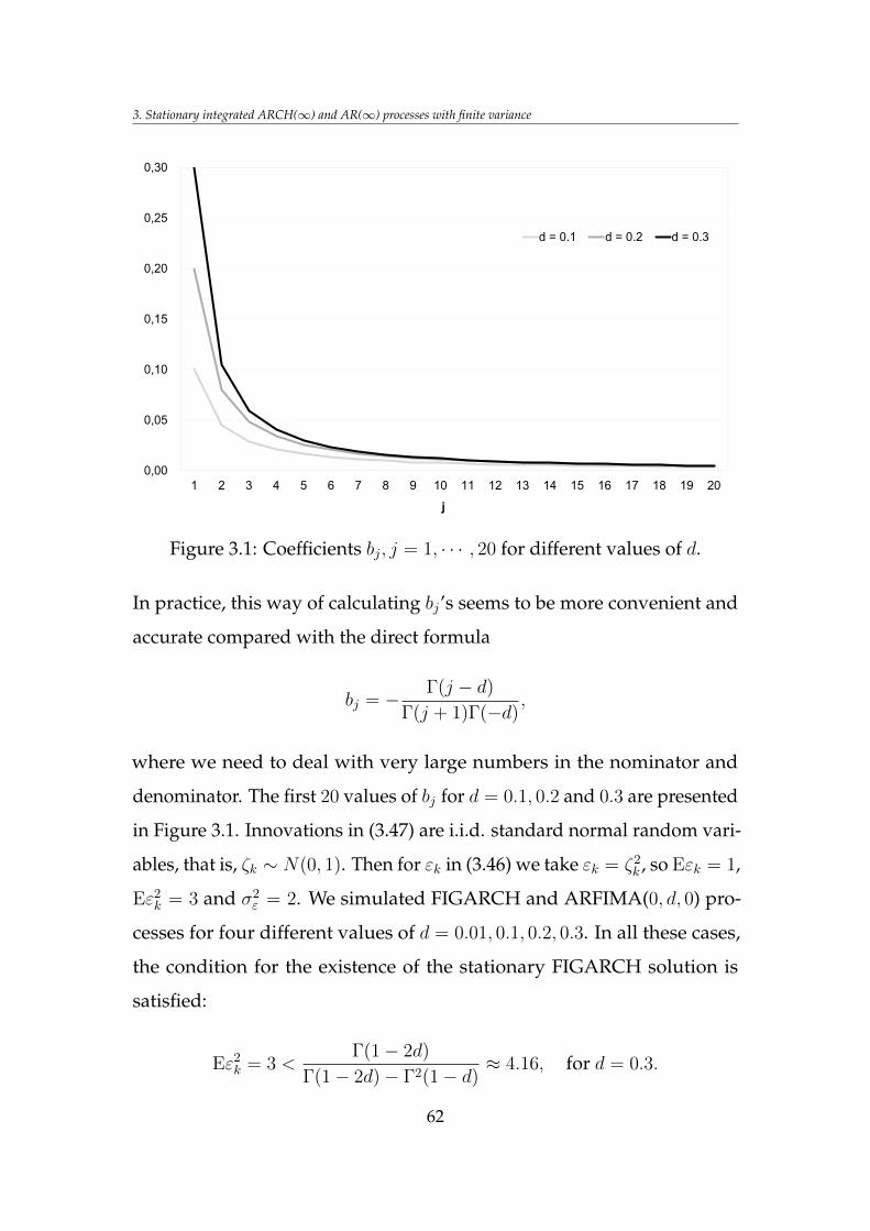
3. Stationary integrated ARCH(∞) and AR(∞) processes with finite variance

0,00

0,05

0,10

0,15

0,20

0,25

0,30

1 2 3 4 5 6 7 8 9 10 11 12 13 14 15 16 17 18 19 20

j

d = 0.1 d = 0.2 d = 0.3

Figure 3.1: Coefficients bj, j = 1, · · · , 20 for different values of d.

In practice, this way of calculating bj’s seems to be more convenient and

accurate compared with the direct formula

bj = − Γ(j − d)

Γ(j + 1)Γ(−d),

where we need to deal with very large numbers in the nominator and

denominator. The first 20 values of bj for d = 0.1, 0.2 and 0.3 are presented

in Figure 3.1. Innovations in (3.47) are i.i.d. standard normal random vari-

ables, that is, ζk ∼ N(0, 1). Then for εk in (3.46) we take εk = ζ2k , so Eεk = 1,

Eε2k = 3 and σ2

ε = 2. We simulated FIGARCH and ARFIMA(0, d, 0) pro-

cesses for four different values of d = 0.01, 0.1, 0.2, 0.3. In all these cases,

the condition for the existence of the stationary FIGARCH solution is

satisfied:

Eε2k = 3 <

Γ(1− 2d)

Γ(1− 2d)− Γ2(1− d)≈ 4.16, for d = 0.3.

62

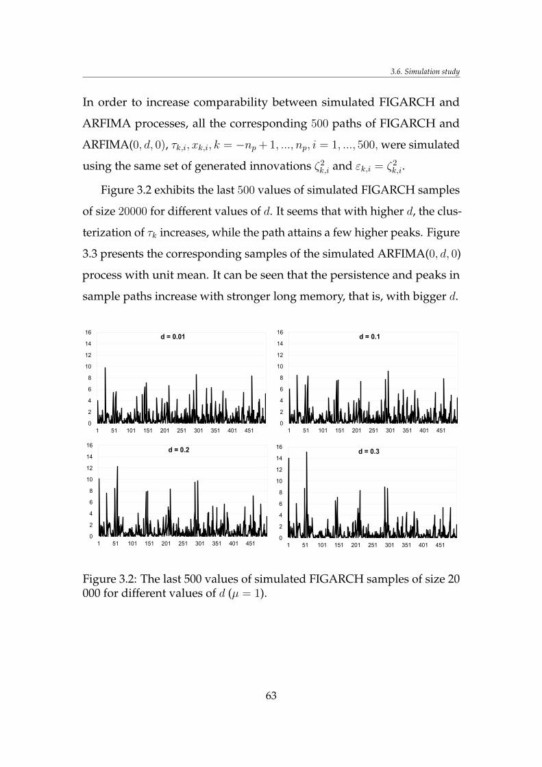
3.6. Simulation study

In order to increase comparability between simulated FIGARCH and

ARFIMA processes, all the corresponding 500 paths of FIGARCH and

ARFIMA(0, d, 0), τk,i, xk,i, k = −np + 1, ..., np, i = 1, ..., 500, were simulated

using the same set of generated innovations ζ2k,i and εk,i = ζ2

k,i.

Figure 3.2 exhibits the last 500 values of simulated FIGARCH samples

of size 20000 for different values of d. It seems that with higher d, the clus-

terization of τk increases, while the path attains a few higher peaks. Figure

3.3 presents the corresponding samples of the simulated ARFIMA(0, d, 0)

process with unit mean. It can be seen that the persistence and peaks in

sample paths increase with stronger long memory, that is, with bigger d.

0

2

4

6

8

10

12

14

16

1 51 101 151 201 251 301 351 401 451

d = 0.01

0

2

4

6

8

10

12

14

16

1 51 101 151 201 251 301 351 401 451

d = 0.1

0

2

4

6

8

10

12

14

16

1 51 101 151 201 251 301 351 401 451

d = 0.2

0

2

4

6

8

10

12

14

16

1 51 101 151 201 251 301 351 401 451

d = 0.3

Figure 3.2: The last 500 values of simulated FIGARCH samples of size 20000 for different values of d (µ = 1).

63

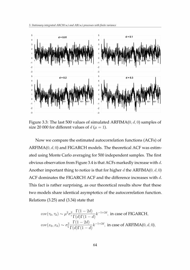
3. Stationary integrated ARCH(∞) and AR(∞) processes with finite variance

-3

-2

-1

0

1

2

3

4

5

1 51 101 151 201 251 301 351 401 451

d = 0.01

-3

-2

-1

0

1

2

3

4

5

1 51 101 151 201 251 301 351 401 451

d = 0.1

-3

-2

-1

0

1

2

3

4

5

1 51 101 151 201 251 301 351 401 451

d = 0.2

-3

-2

-1

0

1

2

3

4

5

1 51 101 151 201 251 301 351 401 451

d = 0.3

Figure 3.3: The last 500 values of simulated ARFIMA(0, d, 0) samples ofsize 20 000 for different values of d (µ = 1).

Now we compare the estimated autocorrelation functions (ACFs) of

ARFIMA(0, d, 0) and FIGARCH models. The theoretical ACF was estim-

ated using Monte Carlo averaging for 500 independent samples. The first

obvious observation from Figure 3.4 is that ACFs markedly increase with d.

Another important thing to notice is that for higher d the ARFIMA(0, d, 0)

ACF dominates the FIGARCH ACF and the difference increases with d.

This fact is rather surprising, as our theoretical results show that these

two models share identical asymptotics of the autocorrelation function.

Relations (3.25) and (3.34) state that

cov(τ0, τk) ∼ µ2σ2z

Γ(1− 2d)

Γ(d)Γ(1− d)k−1+2d, in case of FIGARCH,

cov(x0, xk) ∼ σ2ξ

Γ(1− 2d)

Γ(d)Γ(1− d)k−1+2d, in case of ARFIMA(0, d, 0),

64

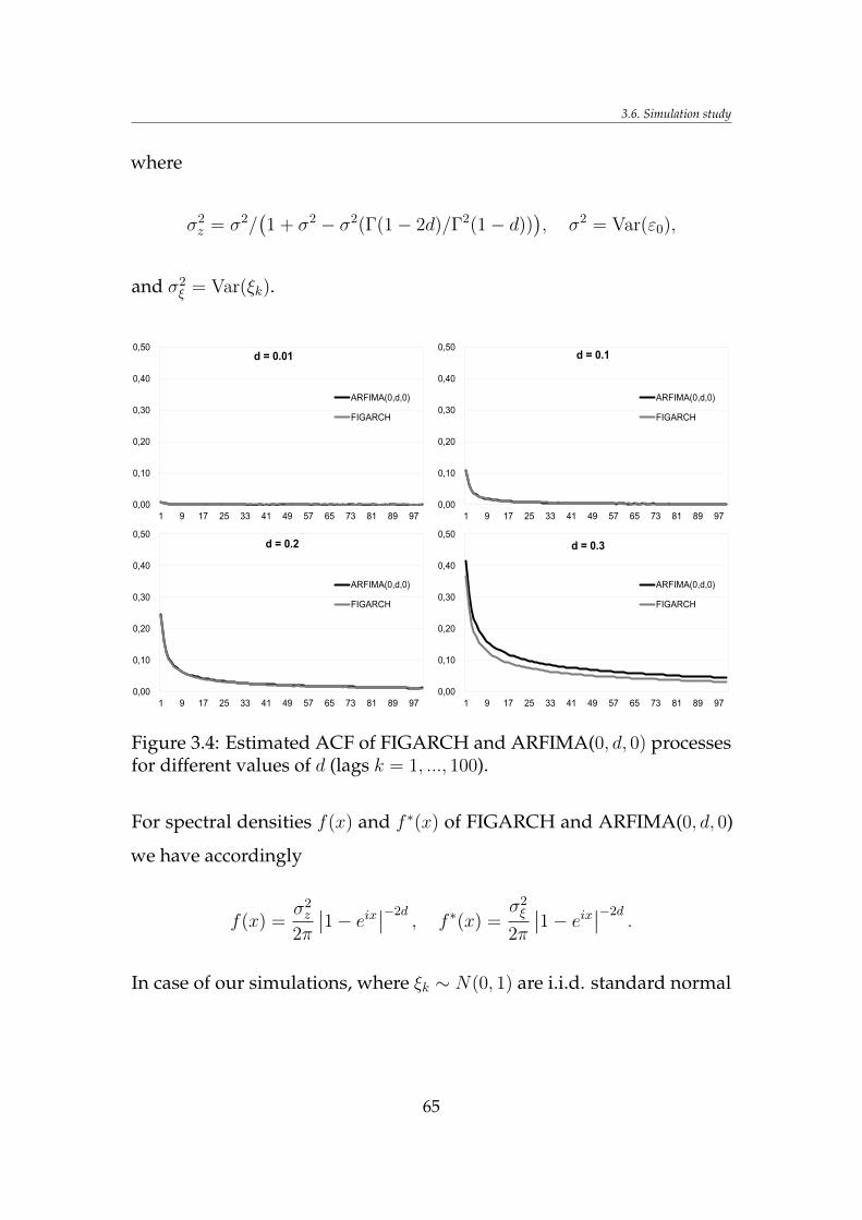
3.6. Simulation study

where

σ2z = σ2/

(1 + σ2 − σ2(Γ(1− 2d)/Γ2(1− d))

), σ2 = Var(ε0),

and σ2ξ = Var(ξk).

0,00

0,10

0,20

0,30

0,40

0,50

1 9 17 25 33 41 49 57 65 73 81 89 97

d = 0.01

ARFIMA(0,d,0)

FIGARCH

0,00

0,10

0,20

0,30

0,40

0,50

1 9 17 25 33 41 49 57 65 73 81 89 97

d = 0.1

ARFIMA(0,d,0)

FIGARCH

0,00

0,10

0,20

0,30

0,40

0,50

1 9 17 25 33 41 49 57 65 73 81 89 97

d = 0.2

ARFIMA(0,d,0)

FIGARCH

0,00

0,10

0,20

0,30

0,40

0,50

1 9 17 25 33 41 49 57 65 73 81 89 97

d = 0.3

ARFIMA(0,d,0)

FIGARCH

Figure 3.4: Estimated ACF of FIGARCH and ARFIMA(0, d, 0) processesfor different values of d (lags k = 1, ..., 100).

For spectral densities f(x) and f ∗(x) of FIGARCH and ARFIMA(0, d, 0)

we have accordingly

f(x) =σ2z

2π

∣∣1− eix∣∣−2d, f∗(x) =

σ2ξ

2π

∣∣1− eix∣∣−2d.

In case of our simulations, where ξk ∼ N(0, 1) are i.i.d. standard normal

65

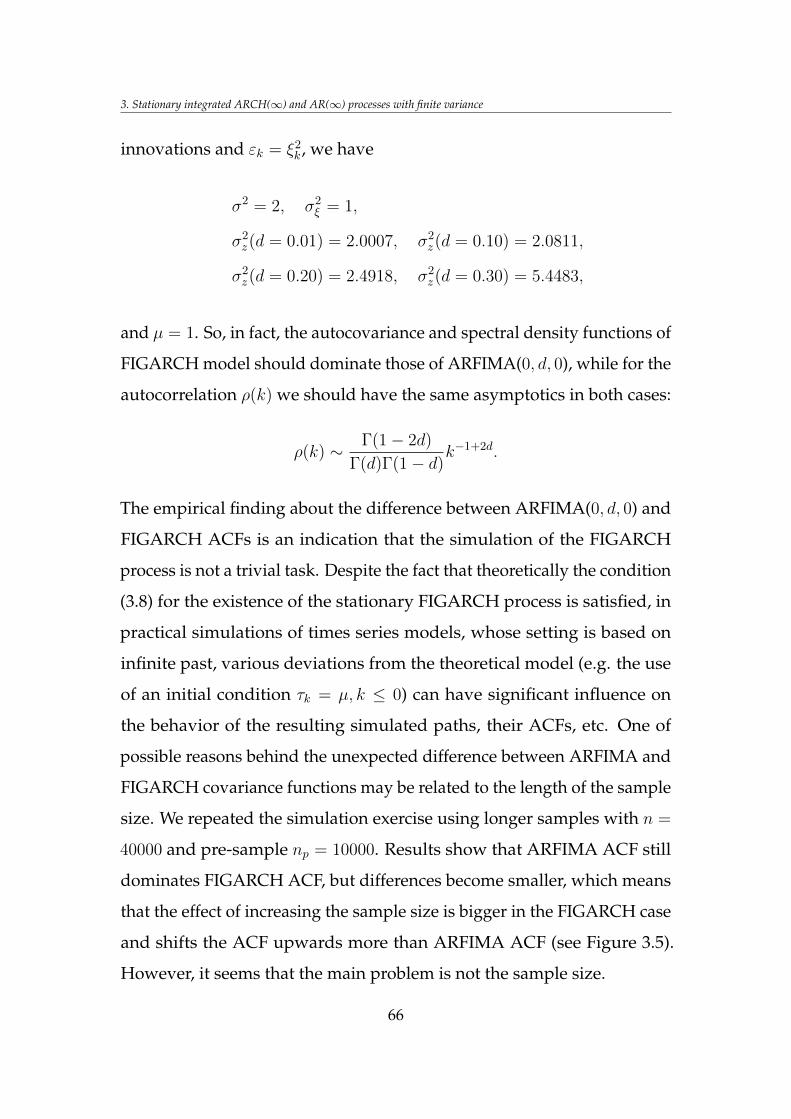
3. Stationary integrated ARCH(∞) and AR(∞) processes with finite variance

innovations and εk = ξ2k, we have

σ2 = 2, σ2ξ = 1,

σ2z(d = 0.01) = 2.0007, σ2

z(d = 0.10) = 2.0811,

σ2z(d = 0.20) = 2.4918, σ2

z(d = 0.30) = 5.4483,

and µ = 1. So, in fact, the autocovariance and spectral density functions of

FIGARCH model should dominate those of ARFIMA(0, d, 0), while for the

autocorrelation ρ(k) we should have the same asymptotics in both cases:

ρ(k) ∼ Γ(1− 2d)

Γ(d)Γ(1− d)k−1+2d.

The empirical finding about the difference between ARFIMA(0, d, 0) and

FIGARCH ACFs is an indication that the simulation of the FIGARCH

process is not a trivial task. Despite the fact that theoretically the condition

(3.8) for the existence of the stationary FIGARCH process is satisfied, in

practical simulations of times series models, whose setting is based on

infinite past, various deviations from the theoretical model (e.g. the use

of an initial condition τk = µ, k ≤ 0) can have significant influence on

the behavior of the resulting simulated paths, their ACFs, etc. One of

possible reasons behind the unexpected difference between ARFIMA and

FIGARCH covariance functions may be related to the length of the sample

size. We repeated the simulation exercise using longer samples with n =

40000 and pre-sample np = 10000. Results show that ARFIMA ACF still

dominates FIGARCH ACF, but differences become smaller, which means

that the effect of increasing the sample size is bigger in the FIGARCH case

and shifts the ACF upwards more than ARFIMA ACF (see Figure 3.5).

However, it seems that the main problem is not the sample size.

66

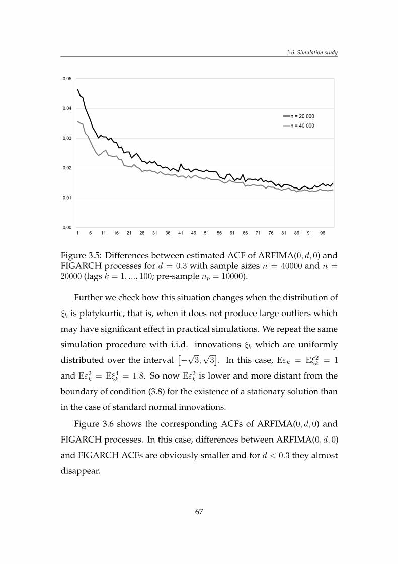
3.6. Simulation study

0,00

0,01

0,02

0,03

0,04

0,05

1 6 11 16 21 26 31 36 41 46 51 56 61 66 71 76 81 86 91 96

n = 20 000

n = 40 000

Figure 3.5: Differences between estimated ACF of ARFIMA(0, d, 0) andFIGARCH processes for d = 0.3 with sample sizes n = 40000 and n =20000 (lags k = 1, ..., 100; pre-sample np = 10000).

Further we check how this situation changes when the distribution of

ξk is platykurtic, that is, when it does not produce large outliers which

may have significant effect in practical simulations. We repeat the same

simulation procedure with i.i.d. innovations ξk which are uniformly

distributed over the interval[−√

3,√

3]. In this case, Eεk = Eξ2

k = 1

and Eε2k = Eξ4

k = 1.8. So now Eε2k is lower and more distant from the

boundary of condition (3.8) for the existence of a stationary solution than

in the case of standard normal innovations.

Figure 3.6 shows the corresponding ACFs of ARFIMA(0, d, 0) and

FIGARCH processes. In this case, differences between ARFIMA(0, d, 0)

and FIGARCH ACFs are obviously smaller and for d < 0.3 they almost

disappear.

67

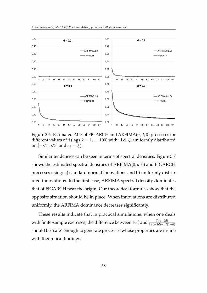
3. Stationary integrated ARCH(∞) and AR(∞) processes with finite variance

0,00

0,10

0,20

0,30

0,40

0,50

1 9 17 25 33 41 49 57 65 73 81 89 97

d = 0.01

ARFIMA(0,d,0)

FIGARCH

0,00

0,10

0,20

0,30

0,40

0,50

1 9 17 25 33 41 49 57 65 73 81 89 97

d = 0.1

ARFIMA(0,d,0)

FIGARCH

0,00

0,10

0,20

0,30

0,40

0,50

1 9 17 25 33 41 49 57 65 73 81 89 97

d = 0.2

ARFIMA(0,d,0)

FIGARCH

0,00

0,10

0,20

0,30

0,40

0,50

1 9 17 25 33 41 49 57 65 73 81 89 97

d = 0.3

ARFIMA(0,d,0)

FIGARCH

Figure 3.6: Estimated ACF of FIGARCH and ARFIMA(0, d, 0) processes fordifferent values of d (lags k = 1, ..., 100) with i.i.d. ζk uniformly distributedon [−

√3,√

3] and εk = ξ2k.

Similar tendencies can be seen in terms of spectral densities. Figure 3.7

shows the estimated spectral densities of ARFIMA(0, d, 0) and FIGARCH

processes using: a) standard normal innovations and b) uniformly distrib-

uted innovations. In the first case, ARFIMA spectral density dominates

that of FIGARCH near the origin. Our theoretical formulas show that the

opposite situation should be in place. When innovations are distributed

uniformly, the ARFIMA dominance decreases significantly.

These results indicate that in practical simulations, when one deals

with finite-sample exercises, the difference between Eε2t and Γ(1−2d)

Γ(1−2d)−Γ2(1−d)

should be "safe" enough to generate processes whose properties are in-line

with theoretical findings.

68

3.6. Simulation study

0

2

4

6

8

10

0,0 0,3 0,7 1,0 1,3 1,6 2,0 2,3 2,6 2,9

Spectral densities with uniformly distributed innovations

ARFIMA(0, d, 0)

FIGARCH

0

2

4

6

8

10

0,0 0,3 0,7 1,0 1,3 1,6 2,0 2,3 2,6 2,9

Spectral densities with normally distributed innovations

ARFIMA(0, d, 0)

FIGARCH

-1

0

1

2

3

0,0 0,2 0,4 0,6 0,8 0,9 1,1

Differences between ARFIMA and FIGARCH spectral densities

With normally distributed innovations

With uniformly distributed innovations

Figure 3.7: Estimated spectral densities of FIGARCH and ARFIMA(0, d, 0)processes for d = 0.3 with i.i.d. ζk a) uniformly distributed on [−

√3,√

3]and b) standard normal, and differences between spectral densities.

3.6.2 IAR(p, d, q) and ARFIMA(p, d, q) processes

In this subsection we explore through simulations the differences between

the classical ARFIMA model

(1− r1L− ...− rpLp)(1− L)dxk = (1 + a1L+ ...+ aqLq)ξk, k ∈ Z,

where R(z) = 1 − r1z − ... − rpzp and A(z) = 1 + a1z + ... + aqz

q, are

polynomials of degrees p, q ≥ 0, respectively, that have no common zeros,

and the IAR(p, d, q) model

xk =∞∑j=1

bjxk−j + ξk + a1ξk−1 + ...+ aqξk−q. (3.48)

69

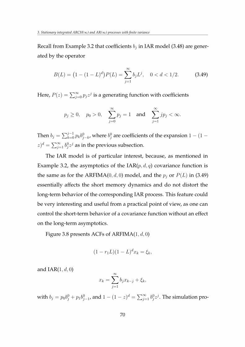
3. Stationary integrated ARCH(∞) and AR(∞) processes with finite variance

Recall from Example 3.2 that coefficients bj in IAR model (3.48) are gener-

ated by the operator

B(L) =(1− (1− L)d

)P (L) =

∞∑j=1

bjLj, 0 < d < 1/2. (3.49)

Here, P (z) =∑∞

j=0 pjzj is a generating function with coefficients

pj ≥ 0, p0 > 0,∞∑j=0

pj = 1 and∞∑j=1

jpj <∞.

Then bj =∑j−1

k=0 pkb0j−k, where b0

j are coefficients of the expansion 1− (1−

z)d =∑∞

j=1 b0jzj as in the previous subsection.

The IAR model is of particular interest, because, as mentioned in

Example 3.2, the asymptotics of the IAR(p, d, q) covariance function is

the same as for the ARFIMA(0, d, 0) model, and the pj or P (L) in (3.49)

essentially affects the short memory dynamics and do not distort the

long-term behavior of the corresponding IAR process. This feature could

be very interesting and useful from a practical point of view, as one can

control the short-term behavior of a covariance function without an effect

on the long-term asymptotics.

Figure 3.8 presents ACFs of ARFIMA(1, d, 0)

(1− r1L)(1− L)dxk = ξk,

and IAR(1, d, 0)

xk =∞∑j=1

bjxk−j + ξk,

with bj = p0b0j + p1b

0j−1, and 1− (1− z)d =

∑∞j=1 b

0jzj . The simulation pro-

70

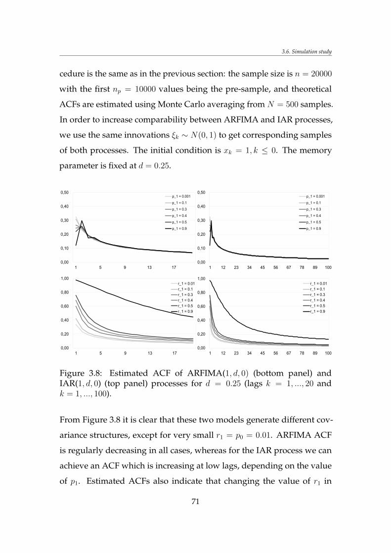
3.6. Simulation study

cedure is the same as in the previous section: the sample size is n = 20000

with the first np = 10000 values being the pre-sample, and theoretical

ACFs are estimated using Monte Carlo averaging from N = 500 samples.

In order to increase comparability between ARFIMA and IAR processes,

we use the same innovations ξk ∼ N(0, 1) to get corresponding samples

of both processes. The initial condition is xk = 1, k ≤ 0. The memory

parameter is fixed at d = 0.25.

0,00

0,20

0,40

0,60

0,80

1,00

1 12 23 34 45 56 67 78 89 100

r_1 = 0.01

r_1 = 0.1

r_1 = 0.3

r_1 = 0.4

r_1 = 0.5

r_1 = 0.9

0,00

0,10

0,20

0,30

0,40

0,50

1 5 9 13 17

p_1 = 0.001

p_1 = 0.1

p_1 = 0.3

p_1 = 0.4

p_1 = 0.5

p_1 = 0.9

0,00

0,10

0,20

0,30

0,40

0,50

1 12 23 34 45 56 67 78 89 100

p_1 = 0.001

p_1 = 0.1

p_1 = 0.3

p_1 = 0.4

p_1 = 0.5

p_1 = 0.9

0,00

0,20

0,40

0,60

0,80

1,00

1 5 9 13 17

r_1 = 0.01

r_1 = 0.1

r_1 = 0.3

r_1 = 0.4

r_1 = 0.5

r_1 = 0.9

Figure 3.8: Estimated ACF of ARFIMA(1, d, 0) (bottom panel) andIAR(1, d, 0) (top panel) processes for d = 0.25 (lags k = 1, ..., 20 andk = 1, ..., 100).

From Figure 3.8 it is clear that these two models generate different cov-

ariance structures, except for very small r1 = p0 = 0.01. ARFIMA ACF

is regularly decreasing in all cases, whereas for the IAR process we can

achieve an ACF which is increasing at low lags, depending on the value

of p1. Estimated ACFs also indicate that changing the value of r1 in

71

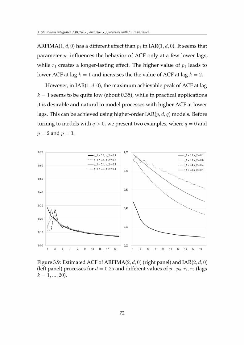
3. Stationary integrated ARCH(∞) and AR(∞) processes with finite variance

ARFIMA(1, d, 0) has a different effect than p1 in IAR(1, d, 0). It seems that

parameter p1 influences the behavior of ACF only at a few lower lags,

while r1 creates a longer-lasting effect. The higher value of p1 leads to

lower ACF at lag k = 1 and increases the the value of ACF at lag k = 2.

However, in IAR(1, d, 0), the maximum achievable peak of ACF at lag

k = 1 seems to be quite low (about 0.35), while in practical applications

it is desirable and natural to model processes with higher ACF at lower

lags. This can be achieved using higher-order IAR(p, d, q) models. Before

turning to models with q > 0, we present two examples, where q = 0 and

p = 2 and p = 3.

0,00

0,10

0,20

0,30

0,40

0,50

0,60

0,70

1 3 5 7 9 11 13 15 17 19

p_1 = 0.1, p_2 = 0.1

p_1 = 0.1, p_2 = 0.8

p_1 = 0.4, p_2 = 0.4

p_1 = 0.8, p_2 = 0.1

0,00

0,20

0,40

0,60

0,80

1,00

1 3 5 7 9 11 13 15 17 19

r_1 = 0.1, r_2 = 0.1

r_1 = 0.1, r_2 = 0.8

r_1 = 0.4, r_2 = 0.4

r_1 = 0.8, r_2 = 0.1

Figure 3.9: Estimated ACF of ARFIMA(2, d, 0) (right panel) and IAR(2, d, 0)(left panel) processes for d = 0.25 and different values of p1, p2, r1, r2 (lagsk = 1, ..., 20).

72

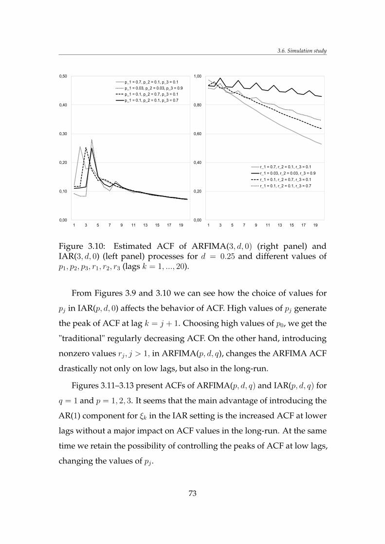
3.6. Simulation study

0,00

0,10

0,20

0,30

0,40

0,50

1 3 5 7 9 11 13 15 17 19

p_1 = 0.7, p_2 = 0.1, p_3 = 0.1

p_1 = 0.03, p_2 = 0.03, p_3 = 0.9

p_1 = 0.1, p_2 = 0.7, p_3 = 0.1

p_1 = 0.1, p_2 = 0.1, p_3 = 0.7

0,00

0,20

0,40

0,60

0,80

1,00

1 3 5 7 9 11 13 15 17 19

r_1 = 0.7, r_2 = 0.1, r_3 = 0.1

r_1 = 0.03, r_2 = 0.03, r_3 = 0.9

r_1 = 0.1, r_2 = 0.7, r_3 = 0.1

r_1 = 0.1, r_2 = 0.1, r_3 = 0.7

Figure 3.10: Estimated ACF of ARFIMA(3, d, 0) (right panel) andIAR(3, d, 0) (left panel) processes for d = 0.25 and different values ofp1, p2, p3, r1, r2, r3 (lags k = 1, ..., 20).

From Figures 3.9 and 3.10 we can see how the choice of values for

pj in IAR(p, d, 0) affects the behavior of ACF. High values of pj generate

the peak of ACF at lag k = j + 1. Choosing high values of p0, we get the

"traditional" regularly decreasing ACF. On the other hand, introducing

nonzero values rj, j > 1, in ARFIMA(p, d, q), changes the ARFIMA ACF

drastically not only on low lags, but also in the long-run.

Figures 3.11–3.13 present ACFs of ARFIMA(p, d, q) and IAR(p, d, q) for

q = 1 and p = 1, 2, 3. It seems that the main advantage of introducing the

AR(1) component for ξk in the IAR setting is the increased ACF at lower

lags without a major impact on ACF values in the long-run. At the same

time we retain the possibility of controlling the peaks of ACF at low lags,

changing the values of pj .

73

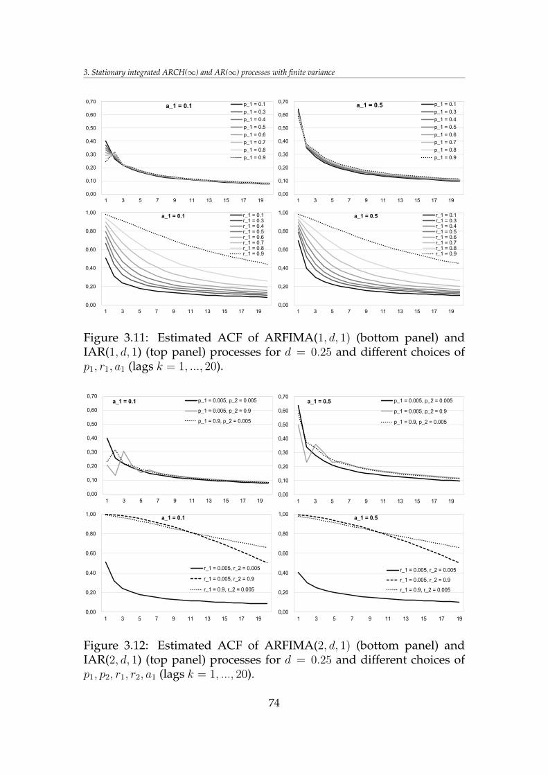
3. Stationary integrated ARCH(∞) and AR(∞) processes with finite variance

0,00

0,10

0,20

0,30

0,40

0,50

0,60

0,70

1 3 5 7 9 11 13 15 17 19

a_1 = 0.1 p_1 = 0.1

p_1 = 0.3

p_1 = 0.4

p_1 = 0.5

p_1 = 0.6

p_1 = 0.7

p_1 = 0.8

p_1 = 0.9

0,00

0,10

0,20

0,30

0,40

0,50

0,60

0,70

1 3 5 7 9 11 13 15 17 19

a_1 = 0.5 p_1 = 0.1

p_1 = 0.3

p_1 = 0.4

p_1 = 0.5

p_1 = 0.6

p_1 = 0.7

p_1 = 0.8

p_1 = 0.9

0,00

0,20

0,40

0,60

0,80

1,00

1 3 5 7 9 11 13 15 17 19

a_1 = 0.1 r_1 = 0.1r_1 = 0.3r_1 = 0.4r_1 = 0.5r_1 = 0.6r_1 = 0.7r_1 = 0.8r_1 = 0.9

0,00

0,20

0,40

0,60

0,80

1,00

1 3 5 7 9 11 13 15 17 19

a_1 = 0.5 r_1 = 0.1r_1 = 0.3r_1 = 0.4r_1 = 0.5r_1 = 0.6r_1 = 0.7r_1 = 0.8r_1 = 0.9

Figure 3.11: Estimated ACF of ARFIMA(1, d, 1) (bottom panel) andIAR(1, d, 1) (top panel) processes for d = 0.25 and different choices ofp1, r1, a1 (lags k = 1, ..., 20).

0,00

0,10

0,20

0,30

0,40

0,50

0,60

0,70

1 3 5 7 9 11 13 15 17 19

a_1 = 0.1 p_1 = 0.005, p_2 = 0.005

p_1 = 0.005, p_2 = 0.9

p_1 = 0.9, p_2 = 0.005

0,00

0,10

0,20

0,30

0,40

0,50

0,60

0,70

1 3 5 7 9 11 13 15 17 19

a_1 = 0.5 p_1 = 0.005, p_2 = 0.005

p_1 = 0.005, p_2 = 0.9

p_1 = 0.9, p_2 = 0.005

0,00

0,20

0,40

0,60

0,80

1,00

1 3 5 7 9 11 13 15 17 19

a_1 = 0.1

r_1 = 0.005, r_2 = 0.005

r_1 = 0.005, r_2 = 0.9

r_1 = 0.9, r_2 = 0.005

0,00

0,20

0,40

0,60

0,80

1,00

1 3 5 7 9 11 13 15 17 19

a_1 = 0.5

r_1 = 0.005, r_2 = 0.005

r_1 = 0.005, r_2 = 0.9

r_1 = 0.9, r_2 = 0.005

Figure 3.12: Estimated ACF of ARFIMA(2, d, 1) (bottom panel) andIAR(2, d, 1) (top panel) processes for d = 0.25 and different choices ofp1, p2, r1, r2, a1 (lags k = 1, ..., 20).

74

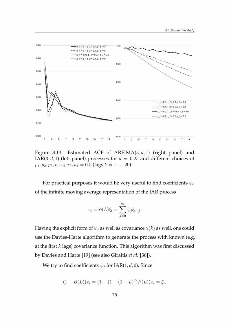
3.6. Simulation study

0,00

0,10

0,20

0,30

0,40

0,50

0,60

0,70

1 3 5 7 9 11 13 15 17 19

p_1 = 0.1, p_2 = 0.1, p_3 = 0.7

p_1 = 0.1, p_2 = 0.7, p_3 = 0.1

p_1 = 0.03, p_2 = 0.03, p_3 = 0.9

p_1 = 0.7, p_2 = 0.1, p_3 = 0.1

0,00

0,20

0,40

0,60

0,80

1,00

1 3 5 7 9 11 13 15 17 19

r_1 = 0.1, r_2 = 0.1, r_3 = 0.7

r_1 = 0.1, r_2 = 0.7, r_3 = 0.1

r_1 = 0.03, r_2 = 0.03, r_3 = 0.9

r_1 = 0.7, r_2 = 0.1, r_3 = 0.1

Figure 3.13: Estimated ACF of ARFIMA(3, d, 1) (right panel) andIAR(3, d, 1) (left panel) processes for d = 0.25 and different choices ofp1, p2, p3, r1, r2, r3, a1 = 0.5 (lags k = 1, ..., 20).

For practical purposes it would be very useful to find coefficients ψk

of the infinite moving average representation of the IAR process

xt = ψ(L)ξt =∞∑j=0

ψjξt−j.

Having the explicit form of ψj as well as covariance γ(k) as well, one could

use the Davies-Harte algorithm to generate the process with known (e.g.

at the first k lags) covariance function. This algorithm was first discussed

by Davies and Harte [19] (see also Giraitis et al. [36]).

We try to find coefficients ψj for IAR(1, d, 0). Since

(1−B(L))xt = (1− (1− (1− L)d)P (L))xt = ξt,

75

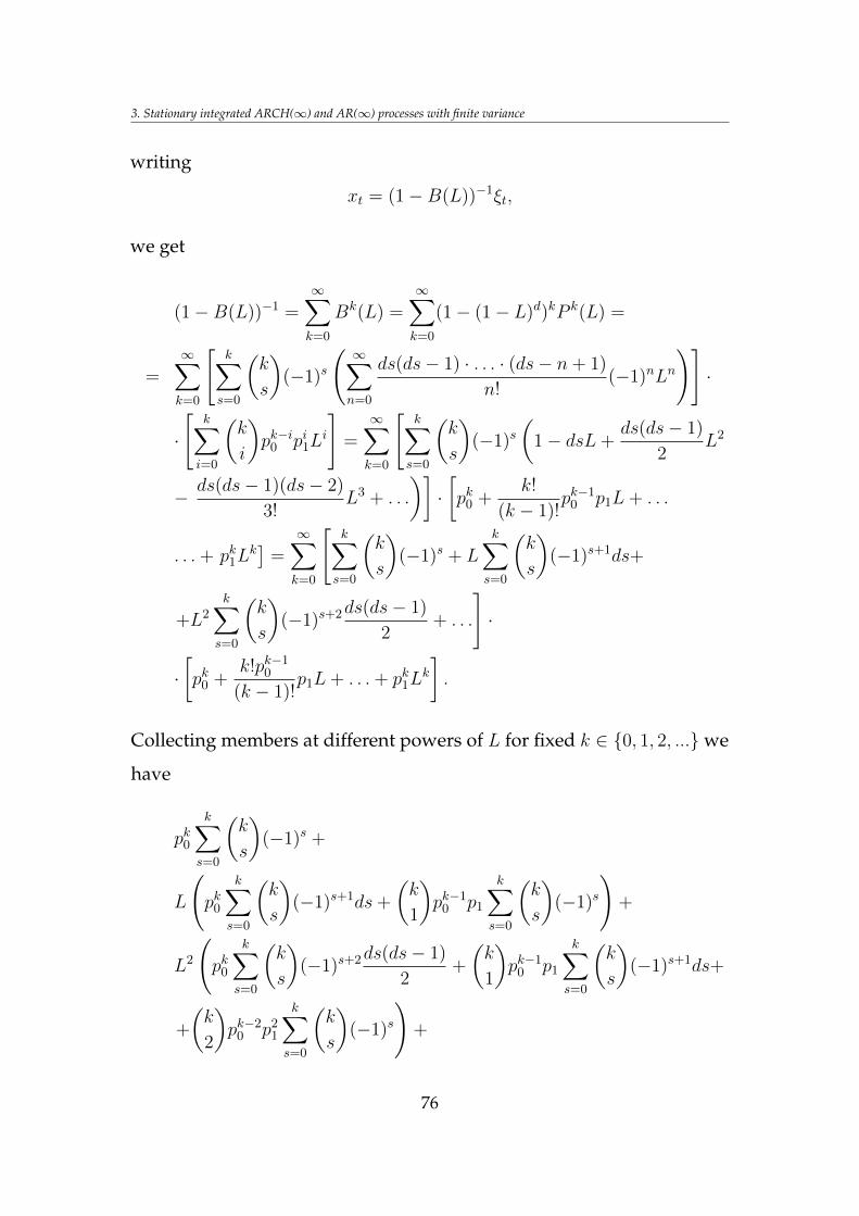
3. Stationary integrated ARCH(∞) and AR(∞) processes with finite variance

writing

xt = (1−B(L))−1ξt,

we get

(1−B(L))−1 =∞∑k=0

Bk(L) =∞∑k=0

(1− (1− L)d)kP k(L) =

=∞∑k=0

[k∑s=0

(k

s

)(−1)s

( ∞∑n=0

ds(ds− 1) · . . . · (ds− n+ 1)

n!(−1)nLn

)]·

·

[k∑i=0

(k

i

)pk−i0 pi1L

i

]=∞∑k=0

[k∑s=0

(k

s

)(−1)s

(1− dsL+

ds(ds− 1)

2L2

− ds(ds− 1)(ds− 2)

3!L3 + . . .

)]·[pk0 +

k!

(k − 1)!pk−1

0 p1L+ . . .

. . .+ pk1Lk]

=∞∑k=0

[k∑s=0

(k

s

)(−1)s + L

k∑s=0

(k

s

)(−1)s+1ds+

+L2k∑s=0

(k

s

)(−1)s+2ds(ds− 1)

2+ . . .

]·

·[pk0 +

k!pk−10

(k − 1)!p1L+ . . .+ pk1L

k

].

Collecting members at different powers of L for fixed k ∈ 0, 1, 2, ...we

have

pk0

k∑s=0

(k

s

)(−1)s +

L

(pk0

k∑s=0

(k

s

)(−1)s+1ds+

(k

1

)pk−1

0 p1

k∑s=0

(k

s

)(−1)s

)+

L2

(pk0

k∑s=0

(k

s

)(−1)s+2ds(ds− 1)

2+

(k

1

)pk−1

0 p1

k∑s=0

(k

s

)(−1)s+1ds+

+

(k

2

)pk−2

0 p21

k∑s=0

(k

s

)(−1)s

)+

76

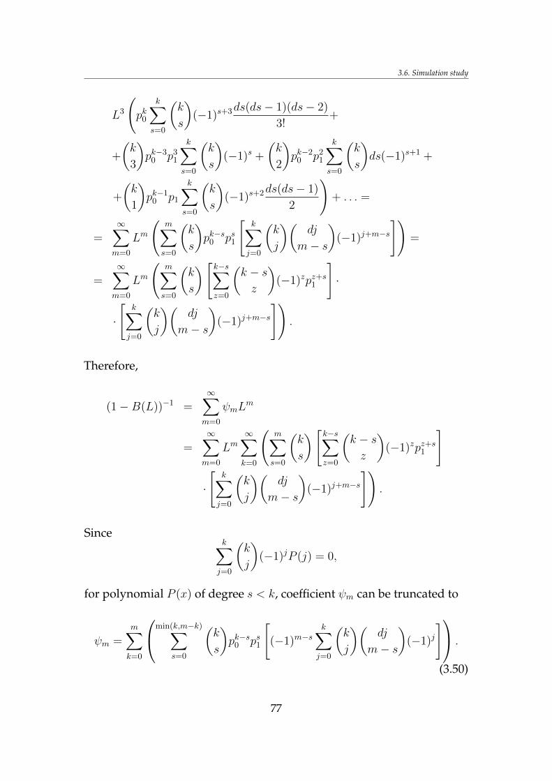
3.6. Simulation study

L3

(pk0

k∑s=0

(k

s

)(−1)s+3ds(ds− 1)(ds− 2)

3!+

+

(k

3

)pk−3

0 p31

k∑s=0

(k

s

)(−1)s +

(k

2

)pk−2

0 p21

k∑s=0

(k

s

)ds(−1)s+1 +

+

(k

1

)pk−1

0 p1

k∑s=0

(k

s

)(−1)s+2ds(ds− 1)

2

)+ . . . =

=∞∑m=0

Lm

(m∑s=0

(k

s

)pk−s0 ps1

[k∑j=0

(k

j

)(dj

m− s

)(−1)j+m−s

])=

=∞∑m=0

Lm

(m∑s=0

(k

s

)[k−s∑z=0

(k − sz

)(−1)zpz+s1

]·

·

[k∑j=0

(k

j

)(dj

m− s

)(−1)j+m−s

]).

Therefore,

(1−B(L))−1 =∞∑m=0

ψmLm

=∞∑m=0

Lm∞∑k=0

(m∑s=0

(k

s

)[k−s∑z=0

(k − sz

)(−1)zpz+s1

]

·

[k∑j=0

(k

j

)(dj

m− s

)(−1)j+m−s

]).

Sincek∑j=0

(k

j

)(−1)jP (j) = 0,

for polynomial P (x) of degree s < k, coefficient ψm can be truncated to

ψm =m∑k=0

min(k,m−k)∑s=0

(k

s

)pk−s0 ps1

[(−1)m−s

k∑j=0

(k

j

)(dj

m− s

)(−1)j

] .

(3.50)

77

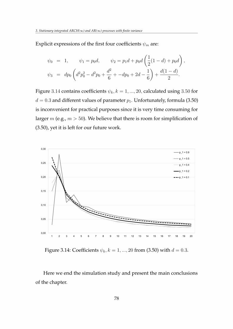
3. Stationary integrated ARCH(∞) and AR(∞) processes with finite variance

Explicit expressions of the first four coefficients ψm are:

ψ0 = 1, ψ1 = p0d, ψ2 = p1d+ p0d

(1

2(1− d) + p0d

),

ψ3 = dp0

(d2p2

0 − d2p0 +d2

6+−dp0 + 2d− 1

6

)+d(1− d)

2.

Figure 3.14 contains coefficients ψk, k = 1, ..., 20, calculated using 3.50 for

d = 0.3 and different values of parameter p1. Unfortunately, formula (3.50)

is inconvenient for practical purposes since it is very time consuming for

larger m (e.g., m > 50). We believe that there is room for simplification of

(3.50), yet it is left for our future work.

0,00

0,05

0,10

0,15

0,20

0,25

0,30

1 2 3 4 5 6 7 8 9 10 11 12 13 14 15 16 17 18 19 20

p_1 = 0.9

p_1 = 0.5

p_1 = 0.4

p_1 = 0.2

p_1 = 0.1

Figure 3.14: Coefficients ψk, k = 1, ..., 20 from (3.50) with d = 0.3.

Here we end the simulation study and present the main conclusions

of the chapter.

78

3.7. Conclusion

3.7 Conclusion

Ding and Granger [20] proposed the Long Memory ARCH model to

capture the hyperbolic decay of sample autocorrelations of speculative

squared returns. The LM ARCH model is closely related to the FIGARCH

model which was independently introduced by Baillie et al. [3]. However,

the existence of a covariance stationary solution of these models was not

established and, thus, the possibility of long memory in the ARCH setting

was doubtful. In this dissertation, we solved this controversy by showing

that FIGARCH and IARCH(∞) equations with zero intercept may have

a nontrivial covariance stationary solution with long memory. We also

obtained necessary and sufficient conditions for the existence of stationary

integrated AR(∞) processes with finite variance and proved that such

processes always have long memory. We provided a complete answer to

the long standing conjecture of Ding and Granger [20] about the existence

of the Long Memory ARCH model.

79

Chapter 4

Quasi-MLE for the

quadratic ARCH model

with long memory

We discuss the parametric quasi-maximum likelihood estimation for the

quadratic ARCH (QARCH) process with long memory, introduced by

Doukhan, Grublyte, and Surgailis [22] and Grublyte and Škarnulis [40]

(see also Chapter 5 of this dissertation), with conditional variance in-

volving the square of inhomogeneous linear combination of an observable

sequence with square summable weights. The above model extends the

QARCH model of Sentana [66] and the Linear ARCH model of Robinson

[62] to the case of strictly positive conditional variance. We prove con-

sistency and asymptotic normality of the corresponding QML estimates,

including the estimate of the long memory parameter 0 < d < 1/2. A

simulation study of empirical MSE is included.

80

4.1. Introduction

4.1 Introduction

Recently, Doukhan et al. [22] and Grublyte and Škarnulis [40] discussed a

class of quadratic ARCH models of the form

rt = ζtσt, σ2t = ω2 +

(a+

∞∑j=1

bjrt−j

)2

+ γσ2t−1, (4.1)

where ζt, t ∈ Z is a standardized i.i.d. sequence, Eζt = 0,Eζ2t = 1, and

γ ∈ [0, 1), ω, a, bj, j ≥ 1, are real parameters satisfying certain conditions,

see Proposition 4.1 below. Grublyte and Škarnulis [40] called (4.1) the

Generalized Quadratic ARCH (GQARCH) model. It is considered in more

detail way in Chapter 5 of this dissertation. By iterating the second equa-

tion in (4.1), the squared volatility in (4.1) can be written as a quadratic

form

σ2t =

∞∑`=0

γ`

ω2 +

(a+

∞∑j=1

bjrt−`−j)2

in lagged variables rt−1, rt−2, ..., and hence it represents a particular case

of Sentana’s [66] Quadratic ARCH model with p = ∞. The model (4.1)

includes the classical Asymmetric GARCH(1,1) process of Engle [25] and

the Linear ARCH (LARCH) model of Robinson [62]:

rt = ζtσt, σt = a+∞∑j=1

bjrt−j. (4.2)

The main interest in (4.1) and (4.2) seems to be the possibility of hav-

ing slowly decaying moving-average coefficients bj with∑∞

j=1 |bj| =

∞,∑∞

j=1 b2j <∞, for modeling long memory in volatility, in which case,

rt and ζt must have zero mean so that the series∑∞

j=1 bjrt−j converges.

81

4. Quasi-MLE for the quadratic ARCH model with long memory

Giraitis et al. [32] proved that the squared stationary solution r2t , t ∈ Z

of the LARCH model in (4.2) with bj decaying as jd−1, 0 < d < 1/2, may

have long memory autocorrelations. In terms of the GQARCH model in

(4.1), similar results were established by Doukhan et al. [22] and Grublyte

and Škarnulis [40]. Namely, assume that parameters γ, ω, a, bj, j ≥ 1, in

(4.1) satisfy

bj ∼ c jd−1 (∃ 0 < d < 1/2, c > 0),

γ ∈ [0, 1), a 6= 0 and

6B2 + 4|µ3|∞∑j=1

|bj|3 + µ4

∞∑j=1

b4j < (1− γ)2, (4.3)

where µp := Eζp0 , p = 1, 2, ..., B2 :=∑∞

j=1 b2j . Then (Grublyte and Škarnulis

[40], Theorems 2.5 and 3.1) there exists a stationary solution of (4.1) with

Er4t <∞, such that

cov(r20, r

2t ) ∼ κ2

1t2d−1, t→∞,

and

n−d−1/2

[ns]∑t=1

(r2t − Er2

t ) →D[0,1] κ2Bd+(1/2)(s), n→∞,

where Bd+(1/2) is a fractional Brownian motion with the Hurst parameter

H = d + (1/2) ∈ (1/2, 1) (see also Definition 2.11) and κi > 0, i = 1, 2,

are some constants;→D[0,1] stands for weak convergence in the Skorohod

space D[0, 1].

As noted by Doukhan et al. [22] and Grublyte and Škarnulis [40], the

GQARCH model of (4.1) and the LARCH model of (4.2) have similar

long memory and leverage properties and can both be used for modeling

82

4.1. Introduction

financial data with the above properties. The main disadvantage of the

latter model in comparison to the former one seems to be the fact that

volatility σt in (4.2) may assume negative values and is not separated from

below by positive constant c > 0 as in the case of (4.1). The standard

quasi-maximum likelihood (QML) approach to the estimation of LARCH

parameters is inconsistent and other estimation methods were developed

by Beran and Schützner [5], Francq and Zakoian [29], Levine et al. [52],

Truquet [68]. The results of Doukhan et al. [22] and Grublyte and Škarnulis

[40] are limited to properties of the stationary solution of (4.1) and do not

include estimation or other statistical inferences for this model.

In this chapter of the dissertation, we discuss the QML estimation for

the 5-parametric GQARCH model

σ2t (θ) =

∞∑`=0

γ`

ω2 +

(a+ c

∞∑j=1

jd−1rt−`−j)2

, (4.4)

depending on parameter θ = (γ, ω, a, d, c), 0 < γ < 1, ω > 0, a 6= 0, c 6= 0

and d ∈ (0, 1/2). The parametric form bj = c jd−1 of moving-average

coefficients in (4.4) is the same as that by Beran and Schützner [5] for the

LARCH model. Similar to Beran and Schützner [5], we discuss the QML

estimator

θn := arg minθ∈Θ

Ln(θ), Ln(θ) :=1

n

n∑t=1

(r2t

σ2t (θ)

+ log σ2t (θ)

),

involving exact conditional variance (4.4) depending on infinite past

rs,−∞ < s < t, and its more realistic version θn := arg minθ∈Θ Ln(θ),

obtained by replacing the σ2t (θ)’s in (4.4) by σ2

t (θ) depending only rs, 1 ≤

s < t (see Section 4.3 for the definition). It should be noted that the QML

83

4. Quasi-MLE for the quadratic ARCH model with long memory

function proposed by Beran and Schützner [5] is modified to avoid the

degeneracy of σ−1t in (4.2), by introducing an additional tuning parameter

ε > 0 which affects the performance of the estimator and whose choice is

a nontrivial task. In terms of the GQARCH model (4.4) with ω > 0, the

aforementioned degeneracy problem does not occur and we deal with un-

modified QMLE in contrast to Beran and Schützner [5]. We also note that

our proofs use techniques different from those of Beran and Schützner [5].

Particularly, the method of orthogonal Volterra expansions of the LARCH

model used by Beran and Schützner [5] is not applicable for model (4.4);

see Doukhan et. al. ([22], Example 1).

Section 4.2 presents some results of Grublyte and Škarnulis [40] about

the existence and properties of the stationary solution of GQARCH equa-

tions in (4.1). More details about the GQARCH process are provided

in Chapter 5 of this dissertation. In Section 4.3, we define several QML

estimators of parameter θ in (4.4). Section 4.4 presents the main results of

this chapter related to consistency and asymptotic normality of the QML

estimators. Finite sample performance of these estimators is investigated

in the simulation study in Section 4.5. Conclusions are summarized in

Section 4.7 and all proofs are relegated to Section 4.6.

4.2 Stationary solution

We recall a few facts from Chapter 5 of this dissertation about the station-

ary solution of (4.1) (see also Grublyte and Škarnulis [40]). First, we give

its definition. Let Ft = σ(ζs, s ≤ t), t ∈ Z, be the sigma-field generated by

ζs, s ≤ t.

84

4.2. Stationary solution

Definition 4.1. By stationary solution of (4.1) we mean a stationary and ergodic

martingale difference sequence rt,Ft, t ∈ Z with Er2t <∞,E[r2

t |Ft−1] = σ2t ,

such that for any t ∈ Z the series Xt :=∑

s<t bt−srs converges in L2, the series

σ2t =

∑∞`=0 γ

`(ω2 + (a+Xt−`)2) converges in L1 and (4.1) holds.

Proposition 4.1. (Grublyte and Škarnulis [40]) Let γ ∈ [0, 1) and ζt, t ∈ Z

be an i.i.d. sequence with zero mean, unit variance and finite moment µp :=

Eζp0 <∞, where p ≥ 2 is an even integer. Assume that

p∑j=2

(p

j

)|µj|

∞∑k=1

|bk|j < (1− γ)p/2. (4.5)

Then there exists a unique stationary solution rt, t ∈ Z of (4.1) such that

the series Xt =∑∞

j=1 bjrt−j converges in Lp and Erpt ≤ C(1 + EXpt ) < ∞.

Moreover, for p = 2, condition (4.5), or

B2 =∞∑j=1

b2j < 1− γ, (4.6)

is necessary and sufficient for the existence of a stationary L2-solution of (4.1)

with

Er2t =

ω2 + a2

1− γ −B2.

Remark 4.1. Condition (4.5) coincides with the corresponding condition

for the LARCH model obtained by Giraitis et al. ([33], Proposition 3). For

p = 4 (4.5) agrees with (4.3).

Remark 4.2. Sufficient conditions for the existence of a stationary solution

of (4.1) with finite moment E|rt|p < ∞ and arbitrary p > 0 are obtained

in Chapter 5 of this dissertation, Theorem 5.1 (see also Grublyte and

85

4. Quasi-MLE for the quadratic ARCH model with long memory

Škarnulis [40], Theorem 2.4). There we extend the corresponding result

of Doukhan et al. ([22], Theorem 1) from γ = 0 to γ > 0. Contrary to

(4.5), the above-mentioned conditions involve absolute constant Kp from

the Burkholder-Rosenthal inequality, which is not known explicitly, and,

therefore, these conditions are not very useful (see Remark 5.2 in Chapter

5 of this dissertation; also Grublyte and Škarnulis ([40]).

4.3 QML Estimators

The following assumptions on the parametric GQARCH model in (4.4)

are imposed.

Assumption (A) ζt, t ∈ Z is a standardized i.i.d. sequence with Eζt =

0,Eζ2t = 1.

Assumption (B) Θ ⊂ R5 is a compact set of parameters θ = (γ, ω, a, d, c)

defined by

(i) γ ∈ [γ1, γ2] with 0 < γ1 < γ2 < 1;

(ii) ω ∈ [ω1, ω2] with 0 < ω1 < ω2 <∞;

(iii) a ∈ [a1, a2] with −∞ < a1 < a2 <∞;

(iv) d ∈ [d1, d2] with 0 < d1 < d2 < 1/2;

(v) c ∈ [c1, c2] with 0 < ci = ci(d, γ) <∞, c1 < c2 such that

B2 = c2∞∑j=1

j2(d−1) < 1− γ

for any c ∈ [c1, c2], γ ∈ [γ1, γ2], d ∈ [d1, d2].

86

4.3. QML Estimators

We assume that the observations rt, 1 ≤ t ≤ n follow the model

in (4.1) with the true parameter θ0 = (γ0, ω0, a0, d0, c0), belonging to the

interior Θ0 of Θ in Assumption (B). The restriction on parameter c in (v) is

due to condition (4.6). The QML estimator of θ ∈ Θ is defined as

θn := arg minθ∈Θ

Ln(θ), (4.7)

where

Ln(θ) =1

n

n∑t=1

(r2t

σ2t (θ)

+ log σ2t (θ)

), (4.8)

and σ2t (θ) is defined in (4.4), that is,

σ2t (θ) =

∞∑`=0

γ`ω2 +

(a+ cYt−`(d)

)2, where (4.9)

Yt(d) :=∞∑j=1

jd−1rt−j.

Note that the definitions in (4.7)–(4.9) depend on (unobserved) rs, s ≤ 0,

and, therefore, the estimator in (4.7) is usually referred to as the QML

estimator given infinite past (see Beran and Schützner [5]). A more realistic

version of (4.7) is defined as

θn := arg minθ∈Θ

Ln(θ), (4.10)

where

Ln(θ) :=1

n

n∑t=1

(r2t

σ2t (θ)

+ log σ2t (θ)

), where (4.11)

σ2t (θ) :=

t−1∑`=0

γ`ω2 +

(a+ cYt−`(d)

)2, Yt(d) :=

t−1∑j=1

jd−1rt−j.

87

4. Quasi-MLE for the quadratic ARCH model with long memory

Note that all quantities in (4.11) depend only on rs, 1 ≤ s ≤ n; hence (4.10)

is called the QML estimator given finite past. The QML functions in (4.8)

and (4.11) can be written as

Ln(θ) =1

n

n∑t=1

lt(θ) and Ln(θ) =1

n

n∑t=1

lt(θ),

respectively, where

lt(θ) :=r2t

σ2t (θ)

+ log σ2t (θ), lt(θ) :=

r2t

σ2t (θ)

+ log σ2t (θ). (4.12)

Finally, following Beran and Schützner [5] we define a truncated version

of (4.10), involving the last O(nβ) quasi-likelihoods lt(θ), n− [nβ] < t ≤ n,

as follows:

θ(β)n := arg min

θ∈ΘL(β)n (θ), L(β)

n (θ) :=1

[nβ]

n∑t=n−[nβ ]+1

lt(θ), (4.13)

where 0 < β < 1 is a "bandwidth parameter". Note that for any t ∈ Z and

θ0 = (γ0, ω0, a0, d0, c0) ∈ Θ, the random functions Yt(d) and Yt(d) in (4.9)

and (4.11) are infinitely differentiable w.r.t. d ∈ (0, 1/2) a.s. Hence, using

the explicit form of σ2t (θ) and σ2

t (θ), it follows that σ2t (θ), σ

2t (θ), lt(θ), lt(θ),

Ln(θ), Ln(θ), L(β)n (θ) and so on, are all infinitely differentiable w.r.t. θ ∈ Θ0

a.s. We use the notation

L(θ) := ELn(θ) = Elt(θ), (4.14)

and

A(θ) := E[∇T lt(θ)∇lt(θ)

], B(θ) := E

[∇T∇lt(θ)

], (4.15)

88

4.4. Main results

where ∇ = (∂/∂θ1, · · · , ∂/∂θ5) and the superscript "T" stands for trans-

posed vector. Particularly, A(θ) andB(θ) are 5×5-matrices. By Lemma 4.1,

the expectations in (4.15) are well-defined for any θ ∈ Θ under condition

Er40 <∞. We have

B(θ) = E[σ−4t (θ)∇Tσ2

t (θ)∇σ2t (θ)] and A(θ) = κ4B(θ), (4.16)

where κ4 := E(ζ20 − 1)2 > 0.

4.4 Main results

Everywhere in this section rt, t ∈ Z is a stationary solution of model

(4.4) as defined in Definition 4.1 and satisfying Assumptions (A) and (B)

of the previous section. As usual, all expectations are taken with respect

to the true value θ0 = (γ0, ω0, a0, d0, c0) ∈ Θ0, where Θ0 is the interior of

the parameter set Θ ⊂ R5.

Theorem 4.1. (i) Let E|rt|3 < ∞. Then θn in (4.7) is a strongly consistent

estimator of θ0, that is,

θna.s.→ θ0.

(ii) Let E|rt|5 <∞. Then θn in (4.7) is asymptotically normal:

n1/2(θn − θ0

) d→ N(0,Σ(θ0)), (4.17)

where Σ(θ0) := B−1(θ0)A(θ0)B−1(θ0) = κ4B−1(θ0) and matrices A(θ), B(θ)

are defined in (4.16).

The following theorem gives asymptotic properties of the "finite past"

89

4. Quasi-MLE for the quadratic ARCH model with long memory

estimators θn and θ(β)n defined in (4.10) and (4.13), respectively.

Theorem 4.2. (i) Let E|rt|3 <∞ and 0 < β < 1. Then

E|θn − θ0| → 0 and E|θ(β)n − θ0| → 0.

(ii) Let E|rt|5 <∞ and 0 < β < 1− 2d0. Then

nβ/2(θ(β)n − θ0)

d→ N(0,Σ(θ0)), (4.18)

where Σ(θ0) is the same as in Theorem 4.1.

The asymptotic results in Theorems 4.1 and 4.2 are similar to the

results of Beran and Schützner ([5], Theorems 1–4) pertaining to the three-

parametric LARCH model in (4.2) with bj = cjd−1, except that Beran and

Schützner [5] deal with a modified QML estimation involving a "tuning

parameter" ε > 0. As explained by Beran and Schützner ([5], Section 3.2),

the convergence rate of∇Ln(θ0) and θn (based on nonstationary truncated

observable series in (4.11)) is, apparently, too slow to guarantee asymptotic

normality, this fact being a consequence of long memory in volatility and

the main reason for introducing estimators θ(β)n in (4.13). Theorems 4.1 and

4.2 are based on subsequent Lemmas 4.1–4.4 which describe properties

of the likelihood processes defined in (4.8), (4.11) and (4.12). As noted in

Section 4.1, our proofs use techniques different from those of Beran and

Schützner [5], which rely on the explicit Volterra series representation of a

stationary solution of the LARCH model.

For multi-index i = (i1, ..., i5) ∈ N5, i 6= 0 = (0, · · · , 0), |i| := i1 + · · ·+

i5, denote partial derivative ∂i := ∂|i|/∏5

j=1 ∂ijθj .

90

4.4. Main results

Lemma 4.1. Let E|rt|p <∞, for some integer p ≥ 1. Then for any i ∈ N5, 0 <

|i| ≤ p,

E supθ∈Θ

∣∣∣∂ilt(θ)∣∣∣ <∞. (4.19)

Moreover, if E|rt|p+ε <∞ for some ε > 0 and p ∈ N, then for any i ∈ N5, 0 ≤

|i| ≤ p,

E supθ∈Θ

∣∣∣∂i (lt(θ)− lt(θ))∣∣∣→ 0, t→∞. (4.20)

Lemma 4.2. The function L(θ), θ ∈ Θ, in (4.14) is bounded and continuous.

Moreover, it attains its unique minimum at θ = θ0.

Lemma 4.3. Let Er40 < ∞. Then matrices A(θ) and B(θ) in (4.15) are well-

defined and strictly positive definite for any θ ∈ Θ.

Write | · | for the Euclidean norm in R5 and in R5 ⊗ R5 (the matrix

norm).

Lemma 4.4. (i) Let E|rt|3 <∞. Then

supθ∈Θ|Ln(θ)− L(θ)| a.s.→ 0 and E sup

θ∈Θ|Ln(θ)− Ln(θ)| → 0. (4.21)

(ii) Let Er4t <∞. Then ∇L(θ) = E∇lt(θ) and

supθ∈Θ|∇Ln(θ)−∇L(θ)| a.s.→ 0 and E sup

θ∈Θ|∇Ln(θ)−∇Ln(θ)| → 0.

(4.22)

(iii) Let E|rt|5 <∞. Then ∇T∇L(θ) = E∇T∇`t(θ) = B(θ) (Equation (4.15))

91

4. Quasi-MLE for the quadratic ARCH model with long memory

and

supθ∈Θ |∇T∇Ln(θ)−∇T∇L(θ)| a.s.→ 0, (4.23)

E supθ∈Θ |∇T∇Ln(θ)−∇T∇Ln(θ)| → 0. (4.24)

Remark 4.3. As noted earlier, the moment conditions of Theorems 4.1 and

4.2 are similar to those of Beran and Schützner [5] for the LARCH model.

Particularly, condition (M′5) of Beran and Schützner ([5], Theorems 2 and 5)

for asymptotic normality of estimators ensures E|rt|5 <∞. This situation

is very different from those of GARCH models where strong consistency

and asymptotic normality of QML estimators hold under virtually no

moment assumption on the observed process; see, for example, Francq

and Zakoian ([28], Chapter 7). The main reason for this difference seems

to be the fact that differentiation with respect to d of Yt(d) =∑∞

j=1 jd−1rt−j

in (4.9) affects all terms of this series and results in "new" long memory

processes ∂iYt(d)/∂di =∑∞

j=1 jd−1(log j)irt−j, i = 1, 2, 3, which are not

bounded by C|Yt(d)| or Cσ2t (θ). Therefore, derivatives of σ−2

t (θ) in (4.9)

are much more difficult to control than in the GARCH case, where these

quantities are bounded; see Francq and Zakoian [28], proof of Theorem 7.2.

Remark 4.4. We expect that our results can be extended to more general

parametric coefficients, for example, fractional filters bj(c, d), j ≥ 1, with

the transfer function∑∞

j=1 e−ijxbj(c, d) = g(c, d)((1−eix)−d−1), x ∈ [−π, π],

where g(c, d) is a smooth function of (c, d) ∈ (0,∞)× (0, 1/2). Particularly,

bj(c, d) := g(c, d)Γ(j + d)

Γ(d)Γ(j + 1)∼ g(c, d)

Γ(d)jd−1, j →∞, (4.25)

and∑∞

j=1 b2j(c, d) = g2(c, d)(Γ(1 − 2d) − Γ2(1 − d))/Γ2(1 − d); see, for

92

4.5. Simulation study

example, Giraitis et al. ([36], Chapter 7). See also Beran and Schützner

([5], Section 2.2). An important condition used in our proofs and satisfied

by bj(c, d) in (4.25) is that partial derivatives ∂idbj(c, d), i = 1, 2, 3, decay

at a similar rate jd−1 (modulus a slowly varying factor). Particularly, for

ARFIMA(0, d, 0) coefficients b0j(d) := Γ(j + d)/Γ(d)Γ(j + 1) =

∏jk=1

d+k−1k ,

it easily follows that

∂db0j(d) = b0

j(d)

j∑k=1

1

d+ k − 1∼ b0

j(d) log j ∼ Γ(d)−1jd−1 log j,

and, similarly,

∂idb0j(d) ∼ b0

j(d)(log j)i ∼ Γ(d)−1jd−1(log j)i, j →∞, i = 2, 3.

4.5 Simulation study

We present a short simulation study of the performance of the QML

estimation for the GQARCH model in (4.4). The GQARCH model in (4.4)

with i.i.d. standard normal innovations ζt was simulated for −m+ 1 ≤

t ≤ m and two sample sizes m = 1000 and m = 5000, using the recurrent

formula in (4.1) with zero initial condition σ−m = 0. The numerical

optimization procedure minimized the QML function:

Lm =1

m

m∑t=1

(r2t

σ2t

+ log σ2t

), (4.26)

93

4. Quasi-MLE for the quadratic ARCH model with long memory

with

rt = ζtσt, σ2t = ω2 +

(a+ c

t+m−1∑j=1

jd−1rt−j

)2

+ γσ2t−1, t = 1, · · · ,m.

(4.27)

The QML function in (4.26) can be viewed as a "realistic proxy" to

the QML function Ln(θ) in (4.13) with m = nβ since (4.26) and (4.27)

similar to (4.13) use "auxiliary" observations in addition to r1, · · · , rmfor computation of m likelihoods in (4.26). However, the number of

"auxiliary" observations in (4.26) equals m and does not grow as m1/β =

n, 0 < β < 1− 2d < 1, in the case of (4.27) and Theorem 4.2 (ii), which is

completely unrealistic. Despite the violation of the condition m = nβ of

Theorem 4.2 (ii) in our simulation study, differences between the sample

root mean square errors (RMSEs) and the theoretical standard deviations

are not vital (and sometimes even insignificant); see Table 4.5 below.

Finite-sample performance of the QML estimator θm minimizing (4.26)

was studied for fixed values of parameters γ0 = 0.7, a0 = −0.2, c0 = 0.2,

and different values of ω0 = 0.1, 0.01, and the long memory parameter

d0 = 0.1, 0.2, 0.3, 0.4. The aforementioned choice of θ0 = (γ0, ω0, a0, d0, c0)

can be explained by an observation that the QML estimation of γ0, a0, c0

appears to be more accurate and stable in comparison with the estimation

of ω0 and d0. The small values of ω0 in our experiment reflect the fact

that in most real data studied by us, the estimated QML value of ω0 was

smaller than 0.05.

The numerical QML minimization was performed using the MATLAB

language for technical computing, under the following constraints:

0.005 ≤ γ ≤ 0.989, 0 ≤ ω ≤ 2, −2 ≤ a ≤ 2, 0 ≤ d ≤ 0.5,

94

4.5. Simulation study

and the value of c in the optimization procedure is chosen in such a way

that would guarantee Assumption (B) (v) with appropriate 0 < ci(d, γ), i =

1, 2.

The results of the simulation experiment are presented in Table 4.5,

which shows the sample RMSEs of the QML estimates θm = (γm, ωm, am,

dm, cm) with 100 independent replications, for two sample lengths m =

1000 and m = 5000 and the aforementioned choices of (γ0, ω0, a0, d0, c0).

The sample RMSEs in Table 4.5 are confronted with standard deviations

(in parantheses) of the infinite past estimator in (4.7) computed according

to Theorem 4.1 (ii) with Σ(θ0) obtained by inverting a simulated matrix

B(θ0)/κ4.

A general impression from Table 4.5 is that theoretical standard devi-

ations (bracketed entries) are generally smaller than the sample RMSEs;

however, these differences become less pronounced with the increase of

m and in some cases (e.g. when ω0 = 0.1,m = 5000) they seem to be

insignificant. Some tendencies in Table 4.5 are quite surprising, partic-

ularly, the decrease of the theoretical standard deviations and most of

sample RMSEs as d0 increases. Also note a sharp increase of theoretical

standard deviations of ωn when ω0 = 0.01, which can be explained by

the fact that the derivative ∂ωσ2t (θ0) = 2ω0/(1 − γ0) becomes very small

with ω0, resulting in a small entry of B(θ0) and a large entry of Σ(θ0). On

the other hand, the RMSEs in Table 4.5 appear to be more stable and less

dependent on θ0 compared with the bracketed entries (in particular this

applies to errors of ωm and dm).

95

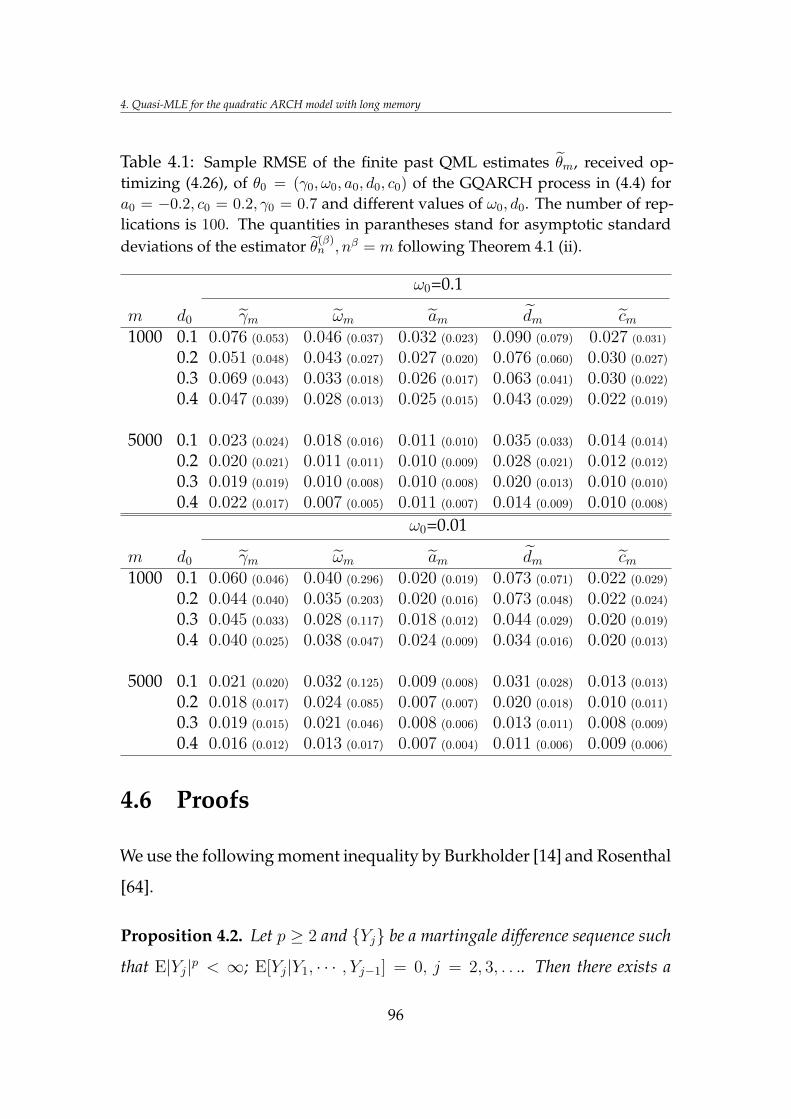
4. Quasi-MLE for the quadratic ARCH model with long memory

Table 4.1: Sample RMSE of the finite past QML estimates θm, received op-timizing (4.26), of θ0 = (γ0, ω0, a0, d0, c0) of the GQARCH process in (4.4) fora0 = −0.2, c0 = 0.2, γ0 = 0.7 and different values of ω0, d0. The number of rep-lications is 100. The quantities in parantheses stand for asymptotic standarddeviations of the estimator θ(β)n , nβ = m following Theorem 4.1 (ii).

ω0=0.1

m d0 γm ωm am dm cm1000 0.1 0.076 (0.053) 0.046 (0.037) 0.032 (0.023) 0.090 (0.079) 0.027 (0.031)

0.2 0.051 (0.048) 0.043 (0.027) 0.027 (0.020) 0.076 (0.060) 0.030 (0.027)

0.3 0.069 (0.043) 0.033 (0.018) 0.026 (0.017) 0.063 (0.041) 0.030 (0.022)

0.4 0.047 (0.039) 0.028 (0.013) 0.025 (0.015) 0.043 (0.029) 0.022 (0.019)

5000 0.1 0.023 (0.024) 0.018 (0.016) 0.011 (0.010) 0.035 (0.033) 0.014 (0.014)

0.2 0.020 (0.021) 0.011 (0.011) 0.010 (0.009) 0.028 (0.021) 0.012 (0.012)

0.3 0.019 (0.019) 0.010 (0.008) 0.010 (0.008) 0.020 (0.013) 0.010 (0.010)

0.4 0.022 (0.017) 0.007 (0.005) 0.011 (0.007) 0.014 (0.009) 0.010 (0.008)

ω0=0.01

m d0 γm ωm am dm cm1000 0.1 0.060 (0.046) 0.040 (0.296) 0.020 (0.019) 0.073 (0.071) 0.022 (0.029)

0.2 0.044 (0.040) 0.035 (0.203) 0.020 (0.016) 0.073 (0.048) 0.022 (0.024)

0.3 0.045 (0.033) 0.028 (0.117) 0.018 (0.012) 0.044 (0.029) 0.020 (0.019)

0.4 0.040 (0.025) 0.038 (0.047) 0.024 (0.009) 0.034 (0.016) 0.020 (0.013)

5000 0.1 0.021 (0.020) 0.032 (0.125) 0.009 (0.008) 0.031 (0.028) 0.013 (0.013)

0.2 0.018 (0.017) 0.024 (0.085) 0.007 (0.007) 0.020 (0.018) 0.010 (0.011)

0.3 0.019 (0.015) 0.021 (0.046) 0.008 (0.006) 0.013 (0.011) 0.008 (0.009)

0.4 0.016 (0.012) 0.013 (0.017) 0.007 (0.004) 0.011 (0.006) 0.009 (0.006)

4.6 Proofs

We use the following moment inequality by Burkholder [14] and Rosenthal

[64].

Proposition 4.2. Let p ≥ 2 and Yj be a martingale difference sequence such

that E|Yj|p < ∞; E[Yj|Y1, · · · , Yj−1] = 0, j = 2, 3, . . .. Then there exists a

96

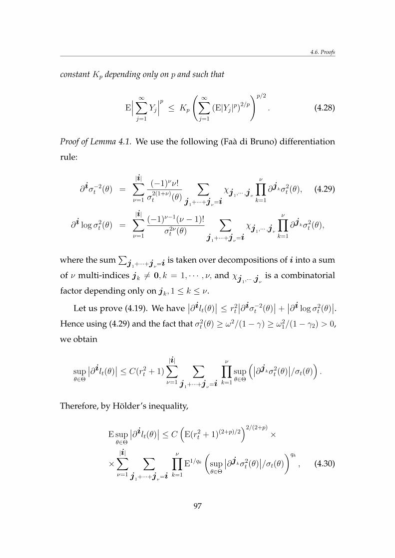
4.6. Proofs

constant Kp depending only on p and such that

E∣∣∣ ∞∑j=1

Yj

∣∣∣p ≤ Kp

( ∞∑j=1

(E|Yj|p)2/p

)p/2

. (4.28)

Proof of Lemma 4.1. We use the following (Faà di Bruno) differentiation

rule:

∂iσ−2t (θ) =

|i|∑ν=1

(−1)νν!

σ2(1+ν)t (θ)

∑j

1+···+j

ν=i

χj1,··· ,j

ν

ν∏k=1

∂jkσ2t (θ), (4.29)

∂i log σ2t (θ) =

|i|∑ν=1

(−1)ν−1(ν − 1)!

σ2νt (θ)

∑j

1+···+j

ν=i

χj1,··· ,j

ν

ν∏k=1

∂jkσ2t (θ),

where the sum∑

j1+···+j

ν=i is taken over decompositions of i into a sum

of ν multi-indices jk 6= 0, k = 1, · · · , ν, and χj1,··· ,j

ν

is a combinatorial

factor depending only on jk, 1 ≤ k ≤ ν.

Let us prove (4.19). We have∣∣∂ilt(θ)∣∣ ≤ r2

t

∣∣∂iσ−2t (θ)

∣∣ +∣∣∂i log σ2

t (θ)∣∣.

Hence using (4.29) and the fact that σ2t (θ) ≥ ω2/(1− γ) ≥ ω2

1/(1− γ2) > 0,

we obtain

supθ∈Θ

∣∣∂ilt(θ)∣∣ ≤ C(r2t + 1)

|i|∑ν=1

∑j

1+···+j

ν=i

ν∏k=1

supθ∈Θ

(∣∣∂jkσ2t (θ)

∣∣/σt(θ)) .Therefore, by Hölder’s inequality,

E supθ∈Θ

∣∣∂ilt(θ)∣∣ ≤ C(

E(r2t + 1)(2+p)/2

)2/(2+p)

×

×|i|∑ν=1

∑j

1+···+j

ν=i

ν∏k=1

E1/qk

(supθ∈Θ

∣∣∂jkσ2t (θ)

∣∣/σt(θ))qk , (4.30)

97

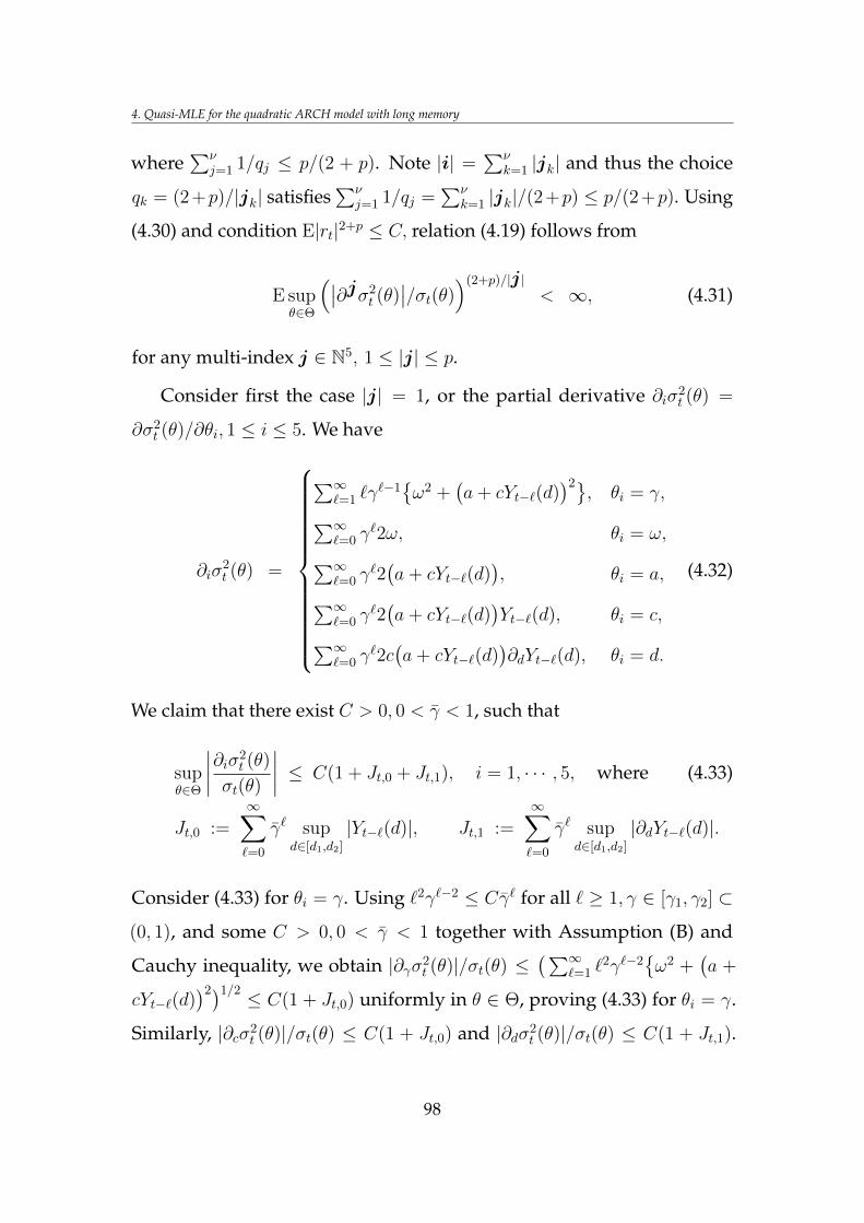
4. Quasi-MLE for the quadratic ARCH model with long memory

where∑ν

j=1 1/qj ≤ p/(2 + p). Note |i| =∑ν

k=1 |jk| and thus the choice

qk = (2+p)/|jk| satisfies∑ν

j=1 1/qj =∑ν

k=1 |jk|/(2+p) ≤ p/(2+p). Using

(4.30) and condition E|rt|2+p ≤ C, relation (4.19) follows from

E supθ∈Θ

(∣∣∂jσ2t (θ)

∣∣/σt(θ))(2+p)/|j |< ∞, (4.31)

for any multi-index j ∈ N5, 1 ≤ |j| ≤ p.

Consider first the case |j| = 1, or the partial derivative ∂iσ2t (θ) =

∂σ2t (θ)/∂θi, 1 ≤ i ≤ 5. We have

∂iσ2t (θ) =

∑∞`=1 `γ

`−1ω2 +

(a+ cYt−`(d)

)2, θi = γ,∑∞

`=0 γ`2ω, θi = ω,∑∞

`=0 γ`2(a+ cYt−`(d)

), θi = a,∑∞

`=0 γ`2(a+ cYt−`(d)

)Yt−`(d), θi = c,∑∞

`=0 γ`2c(a+ cYt−`(d)

)∂dYt−`(d), θi = d.

(4.32)

We claim that there exist C > 0, 0 < γ < 1, such that

supθ∈Θ

∣∣∣∣∂iσ2t (θ)

σt(θ)

∣∣∣∣ ≤ C(1 + Jt,0 + Jt,1), i = 1, · · · , 5, where (4.33)

Jt,0 :=∞∑`=0

γ` supd∈[d1,d2]

|Yt−`(d)|, Jt,1 :=∞∑`=0

γ` supd∈[d1,d2]

|∂dYt−`(d)|.

Consider (4.33) for θi = γ. Using `2γ`−2 ≤ Cγ` for all ` ≥ 1, γ ∈ [γ1, γ2] ⊂

(0, 1), and some C > 0, 0 < γ < 1 together with Assumption (B) and

Cauchy inequality, we obtain |∂γσ2t (θ)|/σt(θ) ≤

(∑∞`=1 `

2γ`−2ω2 +

(a +

cYt−`(d))2)1/2 ≤ C(1 + Jt,0) uniformly in θ ∈ Θ, proving (4.33) for θi = γ.

Similarly, |∂cσ2t (θ)|/σt(θ) ≤ C(1 + Jt,0) and |∂dσ2

t (θ)|/σt(θ) ≤ C(1 + Jt,1).

98

4.6. Proofs

Finally, for θi = ω and θi = a, (4.33) is immediate from (4.32), proving

(4.33).

With (4.33) in mind, (4.31) for |j| = 1 follows from

EJ2+pt,i = E

( ∞∑`=0

γ` supd∈[d1,d2]

|∂idYt−`(d)|)2+p

< ∞, i = 0, 1. (4.34)

Using Minkowski’s inequality and stationarity of Yt(d), we obtain

E1/(2+p)J2+pt,i ≤

∞∑`=0

γ`E1/(2+p) supd|∂idYt−`(d)|2+p

≤ C

(E sup

d|∂idYt(d)|2+p

)1/(2+p)

,

where

∂idYt(d) =∞∑j=1

∂idjd−1rt−j.

Hence, using Beran and Schützner ([5]) Lemma 1 (b) and the inequality

xy ≤ xq/q + yq′/q′, x, y > 0, 1/q + 1/q′ = 1, we obtain

1∑i=0

EJ2+pt,i ≤ C

1∑i=0

E supd∈[d1,d2]

|∂idYt(d)|2+p

≤ C2∑i=0

supd∈[d1,d2]

E|∂idYt(d)|2+p < ∞, (4.35)

since

supd∈[d1,d2]

E|∂idYt(d)|2+p ≤ C supd∈[d1,d2]

( ∞∑j=1

(∂idj

d−1)2 (

E|rt−j|2+p)2/(2+p)

)(2+p)/2

< ∞,

according to condition E|rt|2+p < C, Rosenthal’s inequality in (4.28)

99

4. Quasi-MLE for the quadratic ARCH model with long memory

and the fact that supd∈[d1,d2]

∑∞j=1(∂idj

d−1)2 ≤ supd∈[d1,d2]

∑∞j=1 j

2(d−1)(1 +

log2 j)2 < C, i = 0, 1, 2. This proves (4.31) for |j| = 1.

The proof of (4.31) for 2 ≤ |j| ≤ p is simpler since it reduces to

E supθ∈Θ

∣∣∂jσ2t (θ)

∣∣(p+2)/2< ∞, 2 ≤ |j| ≤ p. (4.36)

Recall θ1 = γ and j ′ := j − (j1, 0, 0, 0, 0) = (0, j2, j3, j4, j5). If j ′ = 0, then

supθ∈Θ

∣∣∂jσ2t (θ)

∣∣ ≤ CJt,0 follows as in (4.33) implying (4.36) as in (4.35)

above. Next, let j ′ 6= 0. Denote

Q2t (θ) := ω2 +

(a+ cYt(d)

)2, (4.37)

so that σ2t (θ) =

∑∞`=0 γ

`Q2t−`(θ). We have withm := j1 ≥ 0 that |∂jσ2

t (θ)| ≤∑∞`=m(`!/(`−m)!)γ`−m |∂j

′

Q2t−`(θ)| and (4.31) follows from

E supθ∈Θ

∣∣∂jQ2t (θ)

∣∣(p+2)/2< ∞. (4.38)

For j2 6= 0 (recall θ2 = ω) the derivative in (4.38) is trivial so that it suffices

to check (4.38) only for j1 = 0. Then applying Faà di Bruno’s rule we get

∣∣∂jQ2t (θ)

∣∣(p+2)/2 ≤ C∑

j1+j

2=j

∣∣∂j1(a+ cYt(d))∣∣(p+2)/2∣∣∂j2(a+ cYt(d))

∣∣(p+2)/2,

and hence, (4.38) reduces to

E supθ∈Θ

∣∣∂j(a+ cYt(d))∣∣p+2

< ∞, 0 ≤ |j| ≤ p,

whose proof is similar to (4.34) above. This ends the proof of (4.19).

The proof of (4.20) is similar. We have |∂i(lt(θ)−lt(θ))| ≤ r2t |∂i(σ−2

t (θ)−

100

4.6. Proofs

σ−2t (θ))|+ |∂i(log σ2

t (θ)− log σ2t (θ))|. Hence, using Hölder’s inequality sim-

ilarly as in the proof of (4.19), it suffices to show

E supθ∈Θ

∣∣∂i(σ−2t (θ)− σ−2

t (θ))∣∣ p+2

p → 0 (4.39)

and

E supθ∈Θ

∣∣∂i(log σ2t (θ)− log σ2

t (θ))∣∣ p+2

p → 0. (4.40)

Below, we prove only the relation (4.39), the proof of (4.40) being analog-

ous.

Using the differentiation rule in (4.29), we have that

∣∣∂i(σ−2t (θ)− σ−2

t (θ))∣∣ ≤ C

|i|∑ν=1

∑j

1+···+j

ν=i

∣∣Wj1,··· ,j

ν

t (θ)− Wj1,··· ,j

ν

t (θ)∣∣,

where

Wj

1,··· ,j

ν

t (θ) := σ−2(1+ν)t (θ)

∏νk=1 ∂

jkσ2

t (θ),

Wj

1,··· ,j

ν

t (θ) := σ−2(1+ν)t (θ)

∏νk=1 ∂

jk σ2

t (θ).

Whence, (4.39) follows from

supθ∈Θ

∣∣Wj1,··· ,j

ν

t (θ)− Wj1,··· ,j

ν

t (θ)∣∣ P→ 0, t→∞ (4.41)

and

E supθ∈Θ

(∣∣Wj1,··· ,j

ν

t (θ)∣∣+∣∣Wj

1,··· ,j

ν

t (θ)∣∣)(p+2+ε)/p

≤ C <∞, (4.42)

101

4. Quasi-MLE for the quadratic ARCH model with long memory

for some constants ε > 0 and C > 0 independent of t. In turn, (4.41) and

(4.42) follow from

supθ∈Θ

∣∣∂j(σ2t (θ)− σ2

t (θ))∣∣ P→ 0, t→∞ (4.43)

and

E supθ∈Θ

(∣∣∂jσ2t (θ)

∣∣/σt(θ))(2+p+ε)/|j |< C, (4.44)

E supθ∈Θ

(∣∣∂j σ2t (θ)

∣∣/σt(θ))(2+p+ε)/|j |< C,

for any multi-index j such that |j| ≥ 0 and 1 ≤ |j| ≤ p, respectively.

Using condition E|rt|2+p+ε < C, relations in (4.44) can be proved

analogously to (4.31), and we omit the details. Consider (4.43). Split

σ2t (θ)− σ2

t (θ) = Ut,1(θ) + Ut,2(θ), where

Ut,1(θ) :=t−1∑`=1

γ`(a+ cYt−`(d)

)2 −(a+ cYt−`(d)

)2, (4.45)

Ut,2(θ) :=∞∑`=t

γ`ω2 +

(a+ cYt−`(d)

)2.

Then supθ∈Θ |∂jUt,i(θ)|P→ 0, t→∞, i = 1, 2, follows by using Assumption

(B) and considering the bounds on the derivatives as in the proof of (4.31).

For instance, let us prove (4.43) for ∂j = ∂d, |j| = 1. We have

∣∣∂dUt,1(θ)∣∣ ≤ C

t−1∑`=1

γ`(

1 +∣∣∣Yt−`(d)

∣∣∣) ∣∣∣∂d (Yt−`(d)− Yt−`(d)) ∣∣∣+

+∣∣∣∂dYt−`(d)

∣∣∣ ∣∣∣Yt−`(d)− Yt−`(d)∣∣∣ .

102

4.6. Proofs

Hence, supθ∈Θ |∂dUt,1(θ)| P→ 0 follows from 0 ≤ γ ≤ γ2 < 1 and

E supd∈[d1,d2]

(∣∣Yt(d)− Yt(d)∣∣2 +

∣∣∂d(Yt(d)− Yt(d))∣∣2) → 0, (4.46)

E supd∈[d1,d2]

(∣∣Yt(d)∣∣2 +

∣∣Yt(d)∣∣2 +

∣∣∂dYt(d)∣∣2 +

∣∣∂dYt(d)∣∣2) ≤ C. (4.47)

The proof of (4.47) mimics that of (4.35) and, therefore, is omitted. To

show (4.46), note Yt(d)− Yt(d) =∑∞

j=t jd−1rt−j and use a similar argument

as in (4.35) to show that the l.h.s. of (4.47) does not exceed

C supd∈[d1,d2]

2∑i=0

E∣∣∂id(Yt(d)− Yt(d))

∣∣2 ≤ C supd∈[d1,d2]

∞∑j=t

j2(d−1)(1 + log2 j

)→ 0,

as t→∞. This proves (4.43) for |j| = 1 and ∂j = ∂d. The remaining cases

in (4.43) follow similarly, and we omit the details. This proves (4.20) and

completes the proof of Lemma 4.1.

Proof of Lemma 4.2. We have

|L(θ1)− L(θ2)| ≤ E|lt(θ1)− lt(θ2)| ≤ CE|σ2t (θ1)− σ2

t (θ2)|,

where the last expectation can be easily shown to vanish as |θ1 − θ2| →

0, θ1, θ2 ∈ Θ. This proves the first statement of the lemma. To show the

second statement of the lemma, write

L(θ)− L(θ0) = E

[σ2t (θ0)

σ2t (θ)

− logσ2t (θ0)

σ2t (θ)

− 1

].

The function f(x) := x − 1 − log x > 0 for x > 0, x 6= 1 and f(x) = 0 if

and only if x = 1. Therefore, L(θ) ≥ L(θ0), ∀ θ ∈ Θ, while L(θ) = L(θ0) is

103

4. Quasi-MLE for the quadratic ARCH model with long memory

equivalent to

σ2t (θ) = σ2

t (θ0) (Pθ0 − a.s.). (4.48)

Thus, it remains to show that (4.48) implies θ = θ0 = (γ0, ω0, a0, d0, c0).

Consider the "projection" Psξ = E[ξ|Fs] − E[ξ|Fs−1] of r.v. ξ, E|ξ| < ∞,

where Fs = σ(ζu, u ≤ s) (see Section 4.2). Equation (4.48) implies

0 = Ps(σ2t (θ)−σ2

t (θ0)) = Ps(Q2t (θ)−Q2

t (θ0))+(γ−γ0)Psσ2t−1(θ0), ∀s ≤ t−1,

(4.49)

where Q2t (θ) = ω2 +

(a+∑

u<t bt−u(θ)ru)2 is the same as in (4.37). We have

PsQ2t (θ) = 2abt−s(θ)rs + 2bt−s(θ)rs

∑u<s

bt−u(θ)ru +∑s≤u<t

b2t−u(θ)Psr

2u

= 2abt−s(θ)ζsσs(θ0) + 2bt−s(θ)ζsσs(θ0)∑u<s

bt−u(θ)ru +

+∑s<u<t

b2t−u(θ)Psσ

2u(θ0) + b2

t−s(θ)(ζ2s − 1)σ2

s(θ0). (4.50)

Whence and from (4.49) for s = t− 1 using Pt−1σ2t−1(θ0) = 0, we obtain

C1(θ, θ0)ζ2t−1 + 2C2(θ, θ0)ζt−1 − C1(θ, θ0) = 0, (4.51)

where

C1(θ, θ0) :=(c2 − c2

0

)σt−1(θ0),

C2(θ, θ0) := (ac− a0c0) +∑u<t−1

(c2(t− u)d−1 − c2

0(t− u)d0−1)ru.

Since Ci(θ, θ0), i = 1, 2, are Ft−2-measurable, (4.51) implies

C1(θ, θ0) = C2(θ, θ0) = 0,

104

4.6. Proofs

particularly, c = c0 since σt−1(θ0) ≥ ω > 0. Then

0 = C2(θ, θ0) = c0(a− a0) + c20

∑u<t−1

((t− u)d−1 − (t− u)d0−1)ru,

and Eru = 0 lead to a = a0 and next to

0 = E

( ∑u<t−1

((t− u)d−1 − (t− u)d0−1

)ru

)2

= Er20

∑j≥2

(jd−1 − jd0−1

)2= 0,

or d = d0. Consequently, Ps(Q2t (θ)−Q2

t (θ0)) = 0 for any s ≤ t−1 and hence

γ = γ0 in view of (4.49). Finally, ω = ω0 follows from Eσ2t (θ) = Eσ2

t (θ0)

and the fact that ω > 0, ω0 > 0. This proves θ = θ0 as well as the lemm.

Proof of Lemma 4.3. From (4.16), it suffices to show that

∇σ2t (θ)λ

T = 0, (4.52)

for some θ ∈ Θ and λ ∈ R5, λ 6= 0 leads to a contradiction. To this end, we

use a similar projection argument as in the proof of Lemma 4.2. First, note

that σ2t (θ) = Q2

t (θ) + γσ2t−1(θ) implies

∇σ2t (θ) =

(0,∇4Q

2t (θ)

)+ γ∇σ2

t−1(θ) + (∇γ)σ2t−1(θ),

where∇4 = (∂/θ2, · · · , ∂θ5). Hence and using the fact that (4.52) holds for

any t ∈ Z by stationarity, from (4.52) we obtain

(σ2t−1(θ),∇4Q

2t (θ)

)λT = 0. (4.53)

Thus,

(Psσ2t−1(θ), Ps∇T

4Q2t (θ))λ = 0, ∀ s ≤ t− 1;

105

4. Quasi-MLE for the quadratic ARCH model with long memory

compare with (4.49). For s = t− 1 using Pt−1σ2t−1(θ) = 0, Pt−1∇4Q

2t (θ) =

∇4Pt−1Q2t (θ) by differentiating (4.50) similarly to (4.51), we obtain

D1(λ)ζ2t−1 + 2D2(λ)ζt−1 −D1(λ) = 0, (4.54)

where D1(λ) := 2λ5σt−1(θ) and

D2(λ) := λ3c+ λ5a+ 2λ5c∑u<t−1

(t− u)d−1ru +

+ λ4c2∑u<t−1

(t− u)d−2 log(t− u)ru,

λ = (λ1, · · · , λ5)T . As in (4.51), Di(λ), i = 1, 2 are Ft−2-measurable, (4.54)

implying Di(λ) = 0, i = 1, 2. Hence, λ5 = 0 and then D2(λ) = 0 reduces

to λ3c + λ4c2∑

u<t−1(t − u)d−2 log(t − u)ru = 0. By taking expectation

and using c 6= 0, we obtain λ3 = 0 and then λ4 = 0 since E(∑

u<t−1(t −

u)d−2 log(t− u)ru)2 6= 0. The aforementioned facts allow rewriting (4.53)

as 2ωλ2 + λ1σ2t−1(θ) = 0. Unless both λ1 and λ2 vanish, the last equation

means that either λ1 6= 0 and σ2t (θ) is a deterministic process, which

contradicts c 6= 0, or λ1 = 0, λ2 6= 0 and ω = 0, which contradicts ω 6= 0.

Lemma 4.3 is proved.

Proof of Lemma 4.4. Consider the first relation in (4.21). The pointwise con-

vergence Ln(θ)a.s.→ L(θ) follows by ergodicity of lt(θ) and the uniform

convergence in (4.21) from E supθ∈Θ |∇lt(θ)| <∞ (cf. Beran and Schützner

[5], proof of Lemma 3), which, in turn, follows from Lemma 4.1 (4.19)

with p = 1. The proof of the second relation in (4.21) is immediate from

Lemma 4.1 (4.20) with p = 0, ε = 1. The proof of statements (ii) and (iii)

using Lemma 4.1 is similar and is omitted.

Proof of Theorem 4.1. (i) Follows from Lemmas 4.2 and 4.4 (i) using standard

106

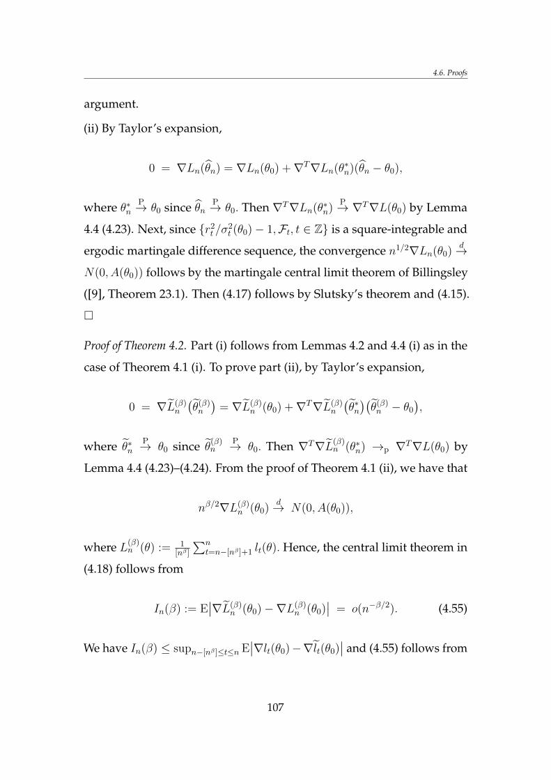
4.6. Proofs

argument.

(ii) By Taylor’s expansion,

0 = ∇Ln(θn) = ∇Ln(θ0) +∇T∇Ln(θ∗n)(θn − θ0),

where θ∗nP→ θ0 since θn

P→ θ0. Then ∇T∇Ln(θ∗n)P→ ∇T∇L(θ0) by Lemma

4.4 (4.23). Next, since r2t /σ

2t (θ0)− 1,Ft, t ∈ Z is a square-integrable and

ergodic martingale difference sequence, the convergence n1/2∇Ln(θ0)d→

N(0, A(θ0)) follows by the martingale central limit theorem of Billingsley

([9], Theorem 23.1). Then (4.17) follows by Slutsky’s theorem and (4.15).

Proof of Theorem 4.2. Part (i) follows from Lemmas 4.2 and 4.4 (i) as in the

case of Theorem 4.1 (i). To prove part (ii), by Taylor’s expansion,

0 = ∇L(β)n

(θ(β)n

)= ∇L(β)

n (θ0) +∇T∇L(β)n

(θ∗n)(θ(β)n − θ0

),

where θ∗nP→ θ0 since θ

(β)n

P→ θ0. Then ∇T∇L(β)n (θ∗n) →p ∇T∇L(θ0) by

Lemma 4.4 (4.23)–(4.24). From the proof of Theorem 4.1 (ii), we have that

nβ/2∇L(β)n (θ0)

d→ N(0, A(θ0)),

where L(β)n (θ) := 1

[nβ ]

∑nt=n−[nβ ]+1 lt(θ). Hence, the central limit theorem in

(4.18) follows from

In(β) := E∣∣∇L(β)

n (θ0)−∇L(β)n (θ0)

∣∣ = o(n−β/2). (4.55)

We have In(β) ≤ supn−[nβ ]≤t≤n E∣∣∇lt(θ0)−∇lt(θ0)

∣∣ and (4.55) follows from

107

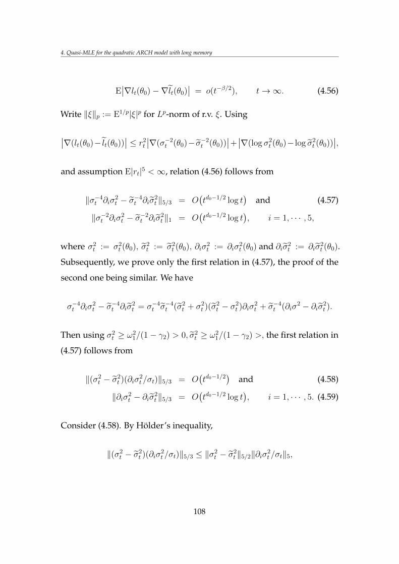
4. Quasi-MLE for the quadratic ARCH model with long memory

E∣∣∇lt(θ0)−∇lt(θ0)

∣∣ = o(t−β/2), t→∞. (4.56)

Write ‖ξ‖p := E1/p|ξ|p for Lp-norm of r.v. ξ. Using

∣∣∇(lt(θ0)− lt(θ0))∣∣ ≤ r2

t

∣∣∇(σ−2t (θ0)− σ−2

t (θ0))∣∣+ ∣∣∇(log σ2

t (θ0)− log σ2t (θ0))

∣∣,and assumption E|rt|5 <∞, relation (4.56) follows from

‖σ−4t ∂iσ

2t − σ−4

t ∂iσ2t ‖5/3 = O

(td0−1/2 log t

)and (4.57)

‖σ−2t ∂iσ

2t − σ−2

t ∂iσ2t ‖1 = O

(td0−1/2 log t

), i = 1, · · · , 5,

where σ2t := σ2

t (θ0), σ2t := σ2

t (θ0), ∂iσ2t := ∂iσ

2t (θ0) and ∂iσ

2t := ∂iσ

2t (θ0).

Subsequently, we prove only the first relation in (4.57), the proof of the

second one being similar. We have

σ−4t ∂iσ

2t − σ−4

t ∂iσ2t = σ−4

t σ−4t (σ2

t + σ2t )(σ

2t − σ2

t )∂iσ2t + σ−4

t (∂iσ2 − ∂iσ2

t ).

Then using σ2t ≥ ω2

1/(1− γ2) > 0, σ2t ≥ ω2

1/(1− γ2) >, the first relation in

(4.57) follows from

‖(σ2t − σ2

t )(∂iσ2t /σt)‖5/3 = O

(td0−1/2

)and (4.58)

‖∂iσ2t − ∂iσ2

t ‖5/3 = O(td0−1/2 log t

), i = 1, · · · , 5. (4.59)

Consider (4.58). By Hölder’s inequality,

‖(σ2t − σ2

t )(∂iσ2t /σt)‖5/3 ≤ ‖σ2

t − σ2t ‖5/2‖∂iσ2

t /σt‖5,

108

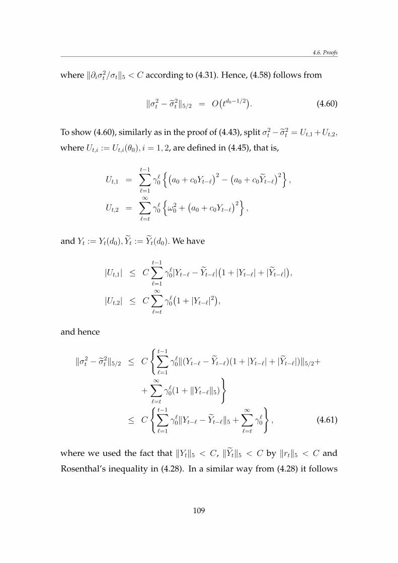
4.6. Proofs

where ‖∂iσ2t /σt‖5 < C according to (4.31). Hence, (4.58) follows from

‖σ2t − σ2

t ‖5/2 = O(td0−1/2

). (4.60)

To show (4.60), similarly as in the proof of (4.43), split σ2t − σ2

t = Ut,1 +Ut,2,

where Ut,i := Ut,i(θ0), i = 1, 2, are defined in (4.45), that is,

Ut,1 =t−1∑`=1

γ`0

(a0 + c0Yt−`

)2 −(a0 + c0Yt−`

)2,

Ut,2 =∞∑`=t

γ`0

ω2

0 +(a0 + c0Yt−`

)2,

and Yt := Yt(d0), Yt := Yt(d0). We have

|Ut,1| ≤ Ct−1∑`=1

γ`0|Yt−` − Yt−`|(1 + |Yt−`|+ |Yt−`|

),

|Ut,2| ≤ C∞∑`=t

γ`0(1 + |Yt−`|2

),

and hence

‖σ2t − σ2

t ‖5/2 ≤ C

t−1∑`=1

γ`0‖(Yt−` − Yt−`)(1 + |Yt−`|+ |Yt−`|)‖5/2+

+∞∑`=t

γ`0(1 + ‖Yt−`‖5)

≤ C

t−1∑`=1

γ`0‖Yt−` − Yt−`‖5 +∞∑`=t

γ`0

, (4.61)

where we used the fact that ‖Yt‖5 < C, ‖Yt‖5 < C by ‖rt‖5 < C and

Rosenthal’s inequality in (4.28). In a similar way from (4.28) it follows

109

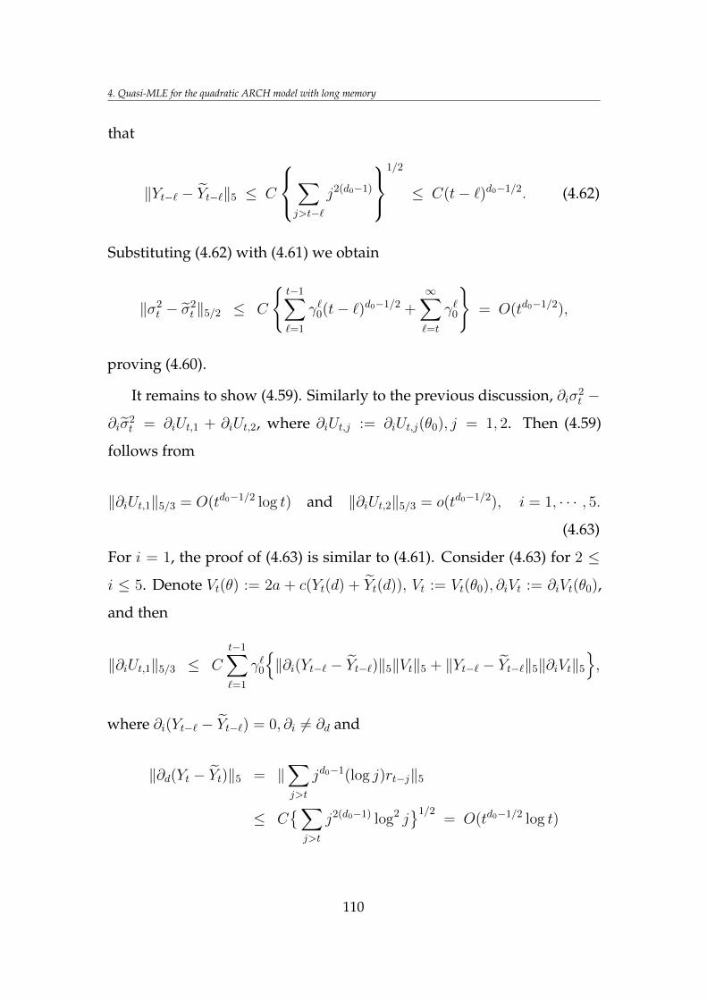
4. Quasi-MLE for the quadratic ARCH model with long memory

that

‖Yt−` − Yt−`‖5 ≤ C

∑j>t−`

j2(d0−1)

1/2

≤ C(t− `)d0−1/2. (4.62)

Substituting (4.62) with (4.61) we obtain

‖σ2t − σ2

t ‖5/2 ≤ C

t−1∑`=1

γ`0(t− `)d0−1/2 +∞∑`=t

γ`0

= O(td0−1/2),

proving (4.60).

It remains to show (4.59). Similarly to the previous discussion, ∂iσ2t −

∂iσ2t = ∂iUt,1 + ∂iUt,2, where ∂iUt,j := ∂iUt,j(θ0), j = 1, 2. Then (4.59)

follows from

‖∂iUt,1‖5/3 = O(td0−1/2 log t) and ‖∂iUt,2‖5/3 = o(td0−1/2), i = 1, · · · , 5.

(4.63)

For i = 1, the proof of (4.63) is similar to (4.61). Consider (4.63) for 2 ≤

i ≤ 5. Denote Vt(θ) := 2a + c(Yt(d) + Yt(d)), Vt := Vt(θ0), ∂iVt := ∂iVt(θ0),

and then

‖∂iUt,1‖5/3 ≤ C

t−1∑`=1

γ`0

‖∂i(Yt−` − Yt−`)‖5‖Vt‖5 + ‖Yt−` − Yt−`‖5‖∂iVt‖5

,

where ∂i(Yt−` − Yt−`) = 0, ∂i 6= ∂d and

‖∂d(Yt − Yt)‖5 = ‖∑j>t

jd0−1(log j)rt−j‖5

≤ C∑j>t

j2(d0−1) log2 j1/2

= O(td0−1/2 log t)

110

4.7. Conclusion

similarly as in (4.62). Hence, the first relation in (4.63) follows from (4.62)

and ‖∂iVt‖5 ≤ C(1 + ‖∂dYt−`‖5 + ‖∂dYt−`‖5) ≤ C < ∞ as in the proof of

(4.59), and the proof of the second relation in (4.63) is analogous. This

proves (4.56) and completes the proof of Theorem 4.2.

4.7 Conclusion

In this chapter we studied the five-parametric QML estimation for a

quadratic ARCH process with long memory and strictly positive con-

ditional variance introduced by Doukhan et al. [22] and Grublyte and

Škarnulis [40], which extends the QARCH model of Sentana [66] and

the Linear ARCH (LARCH) model of Robinson [62]. Following Be-

ran and Schützner [5] who studied a similar problem for the LARCH

model, we discussed several QML estimators of unknown parameter

θ0 ∈ R5 of our model, in particular, an estimator θn depending on obser-

vations rs,−∞ < s ≤ n, from the infinite past, and a class of estimators

θ(β)n , 0 < β < 1, only depending on rs, 1 ≤ s ≤ n, and minimizing the sum

of the last m = nβ = o(n) likelihoods. Under assumptions similar to those

of Beran and Schützner [5], we proved consistency and asymptotic normal-

ity of these estimators with the convergence ratem1/2 = o(n(1−d0)/2), where

d0 ∈ (0, 1/2) is the long memory parameter. However, using estimator

θ(β)n is unrealistic because of the poor and a priori unknown convergence

rate. In the simulation experiment, we studied the empirical performance

of a realistic version of this estimator based on m = n/2 last likelihoods,

for m = 1000 and m = 5000, and show that the empirical RMSEs of this

estimator reflect good agreement with the theoretical standard deviations

with convergence rate m1/2 for m = 5000.

111

Chapter 5

A generalized nonlinear

model for long memory

conditional

heteroscedasticity

In this chapter, we study the existence and properties of a stationary

solution of the ARCH-type equation rt = ζtσt, where ζt are standardized

i.i.d. random variables and the conditional variance satisfies an AR(1)

equation σ2t = Q2

(a +

∑∞j=1 bjrt−j

)+ γσ2

t−1 with a Lipschitz function

Q(x) and real parameters a, γ, bj . We extend the model and the results

by Doukhan, Grublyte and Surgailis [22] from the case γ = 0 to the

case 0 < γ < 1. We also obtain a new condition for the existence of

higher moments of rt, which does not include the Rosenthal constant. In

particular, when Q is the square root of a quadratic polynomial, we prove

112

5.1. Introduction

that rt can exhibit a leverage effect and long memory. The parametric

QML estimation for the latter model (called the Generalized Quadratic

ARCH model, GQARCH) is considered in Chapter 4 of this dissertation.

5.1 Introduction

Doukhan et al. [22] discussed the existence of a stationary solution of the

conditionally heteroscedastic equation

rt = ζtσt, σ2t = Q2

(a+

∞∑j=1

bjrt−j

), (5.1)

where ζt, t ∈ Z are standardized i.i.d. random variables, a, bj , are real

parameters and Q(x) is a Lipschitz function of real variable x ∈ R. The

most important case of (5.1) probably is

Q(x) =√c2 + x2, (5.2)

where c ≥ 0 is a parameter. Models (5.1)–(5.2) include the classical Asym-

metric ARCH(1) of Engle [25] and the Linear ARCH (LARCH) model of

Robinson [62]:

rt = ζtσt, σt = a+∞∑j=1

bjrt−j. (5.3)

Giraitis et al. [32] proved that the squared stationary solution r2t , t ∈ Z

of the LARCH model in Equation (5.3) with bj decaying as jd−1, 0 < d <

1/2, may have long memory autocorrelations. The leverage effect in the

LARCH model was discussed in detail by Giraitis et al. [33]. Doukhan et

113

5. A generalized nonlinear model for long memory conditional heteroscedasticity

al. [22] extended the above properties of the LARCH model (long memory

and leverage) to the model of (5.1)–(5.2) with c > 0, or strictly positive

volatility.

In this chapter, we extend the results of Doukhan et al. [22] to a more

general class of volatility forms:

rt = ζtσt, σ2t = Q2

(a+

∞∑j=1

bjrt−j

)+ γσ2

t−1, (5.4)

where ζt, t ∈ Z, a, bj, Q(x), are as in (5.1) and 0 < γ < 1 is a parameter.

The inclusion of lagged σ2t−1 in (5.4) helps to reduce very sharp peaks and

clustering of volatility which occur in trajectory of models (5.1)–(5.2) near

the threshold c > 0. The generalization from (5.1) to (5.4) is similar to that

from ARCH to GARCH models (see, e.g., Engle [24] and Bollerslev [10]),

particularly, equation (5.4) with Q(x) in (5.2) and bj = 0, j ≥ 2, reduces to

the Asymmetric GARCH(1,1) of Engle [25]:

σ2t = c2 + (a+ brt−1)2 + γσ2

t−1.

Let us describe the main results of this chapter. Section 5.2 (Theorems 5.1

and 5.2) obtains sufficient conditions for the existence of a stationary solu-

tion of (5.4) with E|rt|p <∞ and γ ∈ [0, 1). Theorem 5.1 extends the cor-

responding result by Doukhan et al. [22] (Theorem 4) from γ = 0 to γ > 0.

Theorem 5.2 is new even in the case γ = 0, by providing an explicit suffi-

cient condition (5.24) for higher-order even moments (p = 4, 6, . . . ), which

does not involve the absolute constant in Burkholder-Rosenthal inequality

(5.11). Condition (5.24) coincides with the corresponding moment condi-

tion for the LARCH model and is important for statistical applications, see

114

5.2. Stationary solution

Remark 5.2. Sections 5.3–5.4 deal exclusively with the case of quadratic

Q2 in (5.2), referred to as the Generalized Quadratic ARCH (GQARCH)

model. Theorem 5.3 (Section 5.3) obtains long memory properties of the

squared process r2t , t ∈ Z of the GQARCH model with γ ∈ (0, 1) and

coefficients bj decaying regularly as bj ∼ βjd−1, j →∞, 0 < d < 1/2. Sim-

ilar properties were established by Doukhan et al. [22] for the GQARCH

model with γ = 0 and for the LARCH model (5.3) by Giraitis, Robin-

son and Surgailis [32], Giraitis, Leipus, Robinson and Surgailis [33]. The

quasi-maximum likelihood estimation for the parametric GQARCH model

with long memory was studied in Chapter 4 of this dissertation (see also

Grublyte, Surgailis and Škarnulis [41]). See the review paper by Giraitis,

Leipus and Surgailis [35] and Chapter 3 of this dissertation (also, Giraitis,

Surgailis and Škarnulis [37]) for issues related with long memory ARCH

modeling. Section 5.4 extends to the GQARCH model the leverage effect

discussed by Doukhan et al. [22] and Giraitis et al. [33].

5.2 Stationary solution

Denote |µ|p := E|ζ0|p (p > 0), µp := Eζp0 (p = 1, 2, . . . ) and let

Xt :=∑s<t

bt−srs. (5.5)

Since 0 ≤ γ < 1, equations in (5.4) yield

σ2t =

∞∑`=0

γ`Q2(a+Xt−`) and rt = ζt

√√√√ ∞∑`=0

γ`Q2(a+Xt−`). (5.6)

115

5. A generalized nonlinear model for long memory conditional heteroscedasticity

In other words, stationary solution of (5.4), or

rt = ζt

√√√√ ∞∑`=0

γ`Q2

(a+

∞∑j=1

bjrt−`−j

), (5.7)

can be defined via (5.5), or stationary solution of

Xt :=∑s<t

bt−sζs

√√√√ ∞∑`=0

γ`Q2(a+Xs−`), (5.8)

and vice versa.

In Theorem 5.1, we assume that Q in (5.6) is a Lipschitz function, that

is, there exists a constant LipQ > 0, such that

|Q(x)−Q(y)| ≤ LipQ|x− y|, x, y ∈ R. (5.9)

Note that inequality (5.9) implies the bound

Q2(x) ≤ c21 + c2

2x2, x ∈ R, (5.10)

where c1 ≥ 0, c2 ≥ LipQ and c2 can be chosen arbitrarily close to LipQ.

Let us give some formal definitions. As in Chapter 4, let Ft = σ(ζs, s ≤

t), t ∈ Z, be the sigma-field generated by ζs, s ≤ t. A random process

ut, t ∈ Z is called adapted (respectively, predictable) if ut is Ft-measurable

for each t ∈ Z (respectively, ut is Ft−1-measurable for each t ∈ Z).

Definition 5.1. Let p > 0 be an arbitrary real number.

(i) By Lp-solution of (5.6) or/and (5.7) we mean an adapted process rt, t ∈ Z

with E|rt|p <∞ such that, for any t ∈ Z, the series Xt =∑∞

j=1 bjrt−j converges

116

5.2. Stationary solution

in Lp, the series σ2t =

∑∞`=0 γ

`Q2(a+Xt−`) converges in Lp/2 and (5.7) holds.

(ii) By Lp-solution of (5.8) we mean a predictable process Xt, t ∈ Z with

E|Xt|p < ∞ such that, for any t ∈ Z, the series σ2t =

∑∞`=0 γ

`Q2(a + Xt−`)

converges in Lp/2, the series∑

s<t bt−sζsσs converges in Lp and (5.8) holds.

Define

Bp :=

∑∞

j=1 |bj|p, 0 < p < 2,(∑∞j=1 b

2j

)p/2, p ≥ 2,

Bp,γ :=

Bp/(1− γp/2), 0 < p < 2,

Bp/(1− γ)p/2, p ≥ 2.

Note Bp = Bp,0. Similarly to Doukhan et al. [22], we use the following

moment inequality, see Burkholder [14], Bahr and Esséen [69], Rosenthal

[64].

Proposition 5.1. Let Yj, j ≥ 1 be a sequence of random variables such that

E|Yj|p < ∞ for some p > 0. If p > 1, we additionally assume that Yj is

a martingale difference sequence: E[Yj|Y1, . . . , Yj−1] = 0, j = 2, 3, . . . . Then

there exists a constant Kp ≥ 1 depending only on p and such that

E∣∣∣ ∞∑j=1

Yj

∣∣∣p ≤ Kp

∑∞

j=1 E|Yj|p, 0 < p ≤ 2,(∑∞j=1(E|Yj|p)2/p

)p/2, p > 2.

(5.11)

Proposition 5.2 states that equations (5.7) and (5.8) are equivalent in

the sense that by solving one of these equations, one readily obtains a

solution to the other one.

Proposition 5.2. Let Q be a measurable function satisfying (5.10) with some

c1, c2 ≥ 0, and ζt, t ∈ Z be an i.i.d. sequence with |µ|p = E|ζ0|p < ∞ and

satisfying Eζ0 = 0 for p > 1. In addition, assume Bp <∞ and 0 ≤ γ < 1.

117

5. A generalized nonlinear model for long memory conditional heteroscedasticity

(i) Let Xt, t ∈ Z be a stationary Lp-solution of (5.8) and let

σt :=

√√√√ ∞∑`=0

γ`Q2(a+Xt−`).

Then rt = ζtσt in (5.6) is a stationary Lp-solution of equation (5.7) and

E|rt|p ≤ C(1 + E|Xt|p). (5.12)

Moreover, for p > 1, rt,Ft, t ∈ Z is a martingale difference sequence with

E[rt|Ft−1] = 0, E[|rt|p|Ft−1] = |µ|pσpt . (5.13)

(ii) Let rt, t ∈ Z be a stationary Lp-solution of (5.7). Then Xt, t ∈ Z, defined

in (5.5), is a stationary Lp-solution of equation (5.8) such that

E|Xt|p ≤ CE|rt|p.

Moreover, for p ≥ 2,

E[XtX0] = Er20

∞∑s=1

bt+sbs, t = 0, 1, . . . .

Proof. (i) First, let 0 < p ≤ 2. Then

E|σt|p = E|σ2t |p/2 ≤

∞∑`=0

|γp/2|`E|Q(a+Xt−`)|p <∞.

Hence, using inequality (5.10), the fact that Xt, t ∈ Z is predictable and

|Q(a+Xt−`)|p ≤ |c21 +c2

2(a+Xt−`)|p/2 ≤ C(1+ |a+Xt−`|p) ≤ C(1+ |Xt−`|p),

118

5.2. Stationary solution

we obtain

E|rt|p = |µ|pE|σt|p ≤ C

∞∑`=0

|γp/2|`(1 + E|Xt−`|p)

≤ C(1 + E|Xt|p) < ∞,

proving (5.12) for p ≤ 2. Next, let p > 2. Then

E|σt|p ≤

( ∞∑`=0

γ`E2/p|Q(a+Xt)|p)p/2

≤ CE|Q(a+Xt)|p,

by stationarity and Minkowski’s inequality and hence (5.12) follows using

the same argument as above. Clearly, for p > 1, rt = ζtσt is a mar-

tingale difference sequence and satisfies equations in (5.13). Then, the

convergence in Lp of the series in equation (5.5) follows from (5.12) and

Proposition 5.1:

E∣∣∣ ∞∑j=1

bjrt−j

∣∣∣p ≤ C

∑∞

j=1 |bj|p, 0 < p ≤ 2(∑∞j=1 b

2j

)p/2, p > 2

= CBp < ∞.

In particular,

ζt

√√√√ ∞∑`=0

γ`Q2(a+∑s<t

bt−`−srs) = ζt

√√√√ ∞∑`=0

γ`Q2(a+Xt−`) = rt,

by the definition of rt. Hence, rt, t ∈ Z is a Lp-solution of equation (5.7).

Stationarity of rt, t ∈ Z follows from stationarity of Xt, t ∈ Z.

119

5. A generalized nonlinear model for long memory conditional heteroscedasticity

(ii) Since rt, t ∈ Z is a Lp-solution of equation (5.7), so

rt = ζtσt = ζt

√√√√ ∞∑`=0

γ`Q2(a+Xt−`),

with Xt defined in (5.5) and Xt, t ∈ Z satisfies equation (5.5), where the

series converges in Lp. The rest follows as in Doukhan et al. [22], proof of

Proposition 2.

Remark 5.1. Let p ≥ 2 and |µ|p <∞, then by inequality (5.11), rt, t ∈ Z

being a stationary Lp-solution of (5.6) is equivalent to rt, t ∈ Z being a

stationary L2-solution of (5.6) with E|r0|p <∞. Similarly, if Q and ζt, t ∈

Z satisfy the conditions of Proposition 5.2 and p ≥ 2, then Xt, t ∈ Z,

being a stationary Lp-solution of (5.5), is equivalent to Xt, t ∈ Z being a

stationary L2-solution of (5.5) with E|X0|p < ∞. See also Doukhan et al.

[22], Remark 1.

Theorem 5.1. Let ζt, t ∈ Z satisfy the conditions of Proposition 5.2 and Q

satisfy the Lipschitz condition in (5.9).

(i) Let p > 0 and

K1/pp |µ|1/pp LipQB

1/pp,γ < 1, (5.14)

where Kp is the absolute constant from the moment inequality in (5.11). Then

there exists a unique stationary Lp-solution Xt, t ∈ Z of (5.8) and

E|Xt|p ≤C(p,Q)|µ|pBp

1−Kp|µ|pLippQBp,γ, (5.15)

where C(p,Q) <∞ depends only on p and c1, c2 in inequality (5.10).

(ii) Assume, in addition, that Q2(x) = c21 + c2

2x2, where ci ≥ 0, i = 1, 2, and

120

5.2. Stationary solution

µ2 = Eζ20 = 1. Then c2

2B2,γ < 1 is a necessary and sufficient condition for the

existence of a stationary L2-solution Xt, t ∈ Z of equation (5.8) with a 6= 0.

Proof. (i) We follow the proof of Theorem 4 by Doukhan et al. [22]. For

n ∈ N we recurrently define a solution of equation (5.8) with zero initial

condition at t ≤ −n as

X(n)t :=

0, t ≤ −n,∑t−1s=−n bt−sζsσ

(n)s , t > −n, t ∈ Z,

(5.16)

where σ(n)s :=

√∑n+s`=0 γ

`Q2(a+X(n)s−`). Let us show that X(n)

t , t ∈ Z

converges in Lp to a stationary Lp-solution Xt, t ∈ Z as n→∞.

First, let 0 < p ≤ 2. Let m > n ≥ 0. Then, by inequality (5.11), for any

t > −m we have that

E|X(m)t −X(n)

t |p ≤ Kp|µ|p ∑−m≤s<−n

|bt−s|pE|σ(m)s |p +

+∑−n≤s<t

|bt−s|pE|σ(m)s − σ(n)

s |p

=: Kp|µ|pS ′m,n + S ′′m,n

. (5.17)

Using |Q(a+ x)|p ≤ C + cp3|x|p, x ∈ R, with c3 > c2 > LipQ arbitrarily close

to LipQ, see Doukhan et al. [22], proof of Theorem 4, we obtain

S ′m,n ≤∑

−m≤s<−n|bt−s|p

m+s∑`=0

γp`/2(C + cp3E|X(m)

s−` |p). (5.18)

Next, using |(∑

i>0 γix2i )

1/2 − (∑

i>0 γiy2i )

1/2| ≤ (∑

i>0 γi(xi − yi)2)1/2 we

121

5. A generalized nonlinear model for long memory conditional heteroscedasticity

obtain

|σ(m)s − σ(n)

s | ≤

(s+n∑`=0

γ`(Q(a+X

(m)s−` )−Q(a+X

(n)s−`)

)2+

+s+m∑

`=s+n+1

γ`Q2(a+X(m)s−` )

)1/2

. (5.19)

Hence from the Lipschitz condition in (5.9) we have that

S ′′m,n ≤∑−n≤s<t

|bt−s|p(s+n∑`=0

γp`/2LippQE|X(m)s−` −X

(n)s−`|

p+

+s+m∑

`=s+n+1

γp`/2(C + cp3E|X(m)s−` )|

p)

).

Combining (5.17) and the above bounds, we obtain

E|X(m)t −X(n)

t |p ≤ Kp|µ|p

(cp3

∑−m≤s<t

|bt−s|ps+m∑`=0

γp`/2E|X(m)s−` −X

(n)s−`|

p

+ C∑

−m≤s<−n|bt−s|p

s+m∑`=0

γp`/2+

+ C∑−n≤s<t

|bt−s|ps+m∑

`=s+n+1

γp`/2

)≤ CKp|µ|pκpt+n,γ +

+ Kp|µ|pcp3∑

−m≤s<tbpt−s,γE|X(n)

s −X(m)s |p, (5.20)

where bps,γ :=∑s−1

j=0 γjp/2|bs−j|p, s ≥ 0, and

κt+n := C(1− γp/2)−1Kp|µ|p

( ∑j>t+n

|bj|p + bpt+n,γ

)→ 0 (n→∞).

122

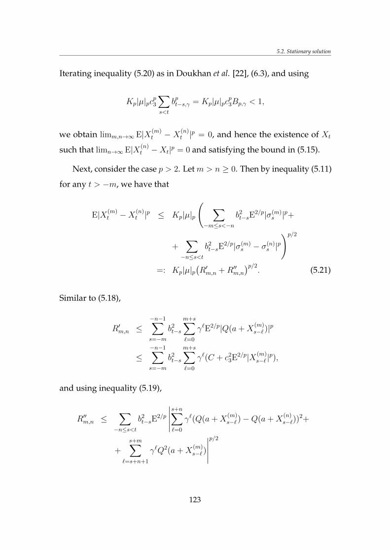
5.2. Stationary solution

Iterating inequality (5.20) as in Doukhan et al. [22], (6.3), and using

Kp|µ|pcp3∑s<t

bpt−s,γ = Kp|µ|pcp3Bp,γ < 1,

we obtain limm,n→∞ E|X(m)t − X(n)

t |p = 0, and hence the existence of Xt

such that limn→∞ E|X(n)t −Xt|p = 0 and satisfying the bound in (5.15).

Next, consider the case p > 2. Let m > n ≥ 0. Then by inequality (5.11)

for any t > −m, we have that

E|X(m)t −X(n)

t |p ≤ Kp|µ|p

( ∑−m≤s<−n

b2t−sE

2/p|σ(m)s |p+

+∑−n≤s<t

b2t−sE

2/p|σ(m)s − σ(n)

s |p)p/2

=: Kp|µ|p(R′m,n +R′′m,n

)p/2. (5.21)

Similar to (5.18),

R′m,n ≤−n−1∑s=−m

b2t−s

m+s∑`=0

γ`E2/p|Q(a+X(m)s−` )|

p

≤−n−1∑s=−m

b2t−s

m+s∑`=0

γ`(C + c23E2/p|X(m)

s−` |p),

and using inequality (5.19),

R′′m,n ≤∑−n≤s<t

b2t−sE

2/p

∣∣∣∣∣s+n∑`=0

γ`(Q(a+X(m)s−` )−Q(a+X

(n)s−`))

2+

+s+m∑

`=s+n+1

γ`Q2(a+X(m)s−` )

∣∣∣∣∣p/2

123

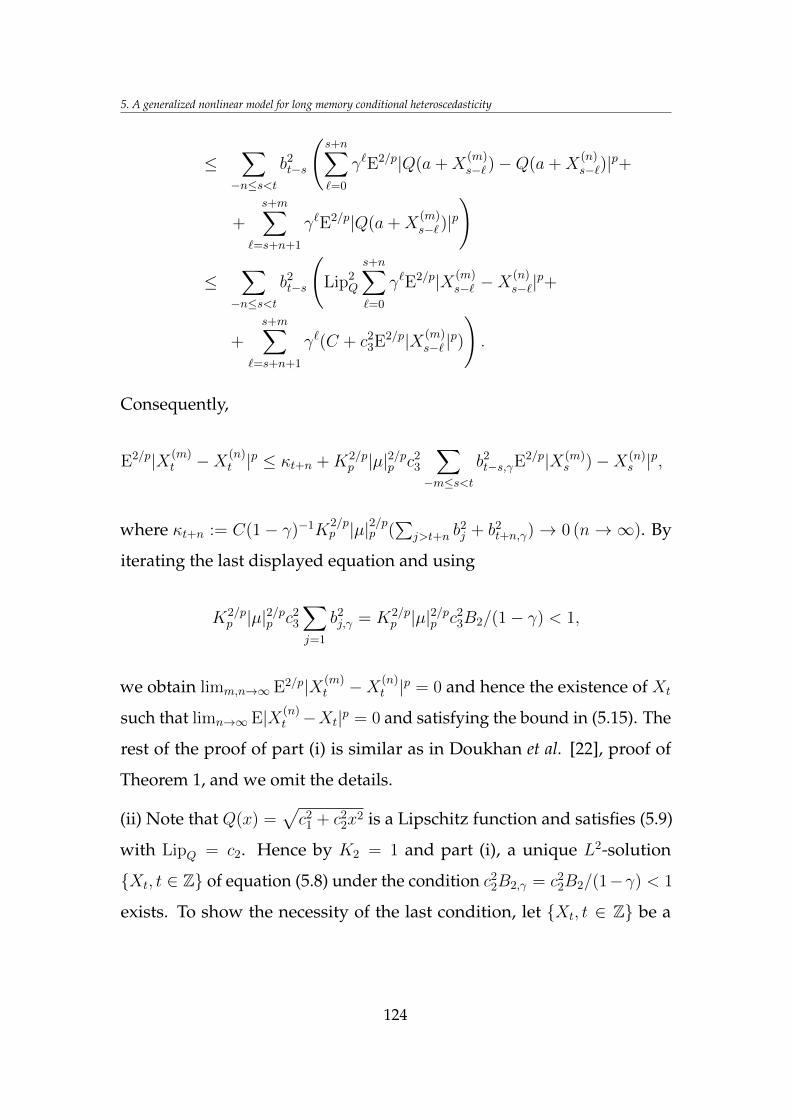
5. A generalized nonlinear model for long memory conditional heteroscedasticity

≤∑−n≤s<t

b2t−s

(s+n∑`=0

γ`E2/p|Q(a+X(m)s−` )−Q(a+X

(n)s−`)|

p+

+s+m∑

`=s+n+1

γ`E2/p|Q(a+X(m)s−` )|

p

)

≤∑−n≤s<t

b2t−s

(Lip2

Q

s+n∑`=0

γ`E2/p|X(m)s−` −X

(n)s−`|

p+

+s+m∑

`=s+n+1

γ`(C + c23E2/p|X(m)

s−` |p)

).

Consequently,

E2/p|X(m)t −X(n)

t |p ≤ κt+n +K2/pp |µ|2/pp c2

3

∑−m≤s<t

b2t−s,γE

2/p|X(m)s )−X(n)

s |p,

where κt+n := C(1− γ)−1K2/pp |µ|2/pp (

∑j>t+n b

2j + b2

t+n,γ)→ 0 (n→∞). By

iterating the last displayed equation and using

K2/pp |µ|2/pp c2

3

∑j=1

b2j,γ = K2/p

p |µ|2/pp c23B2/(1− γ) < 1,

we obtain limm,n→∞ E2/p|X(m)t −X(n)

t |p = 0 and hence the existence of Xt

such that limn→∞ E|X(n)t −Xt|p = 0 and satisfying the bound in (5.15). The

rest of the proof of part (i) is similar as in Doukhan et al. [22], proof of

Theorem 1, and we omit the details.

(ii) Note that Q(x) =√c2

1 + c22x

2 is a Lipschitz function and satisfies (5.9)

with LipQ = c2. Hence by K2 = 1 and part (i), a unique L2-solution

Xt, t ∈ Z of equation (5.8) under the condition c22B2,γ = c2

2B2/(1−γ) < 1

exists. To show the necessity of the last condition, let Xt, t ∈ Z be a

124

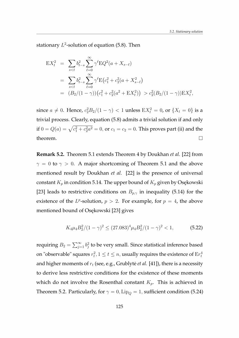
5.2. Stationary solution

stationary L2-solution of equation (5.8). Then

EX2t =

∑s<t

b2t−s

∞∑`=0

γ`EQ2(a+Xs−`)

=∑s<t

b2t−s

∞∑`=0

γ`E(c2

1 + c22(a+X2

s−`)

= (B2/(1− γ))(c2

1 + c22(a2 + EX2

t ))> c2

2(B2/(1− γ))EX2t ,

since a 6= 0. Hence, c22B2/(1 − γ) < 1 unless EX2

t = 0, or Xt = 0 is a

trivial process. Clearly, equation (5.8) admits a trivial solution if and only

if 0 = Q(a) =√c2

1 + c22a

2 = 0, or c1 = c2 = 0. This proves part (ii) and the

theorem.

Remark 5.2. Theorem 5.1 extends Theorem 4 by Doukhan et al. [22] from

γ = 0 to γ > 0. A major shortcoming of Theorem 5.1 and the above

mentioned result by Doukhan et al. [22] is the presence of universal

constantKp in condition 5.14. The upper bound ofKp given by Osekowski

[23] leads to restrictive conditions on Bp,γ in inequality (5.14) for the

existence of the Lp-solution, p > 2. For example, for p = 4, the above

mentioned bound of Osekowski [23] gives

K4µ4B22/(1− γ)2 ≤ (27.083)4µ4B

22/(1− γ)2 < 1, (5.22)

requiring B2 =∑∞

j=1 b2j to be very small. Since statistical inference based

on "observable" squares r2t , 1 ≤ t ≤ n, usually requires the existence of Er4

t

and higher moments of rt (see, e.g., Grublyte et al. [41]), there is a necessity

to derive less restrictive conditions for the existence of these moments

which do not involve the Rosenthal constant Kp. This is achieved in

Theorem 5.2. Particularly, for γ = 0,LipQ = 1, sufficient condition (5.24)

125

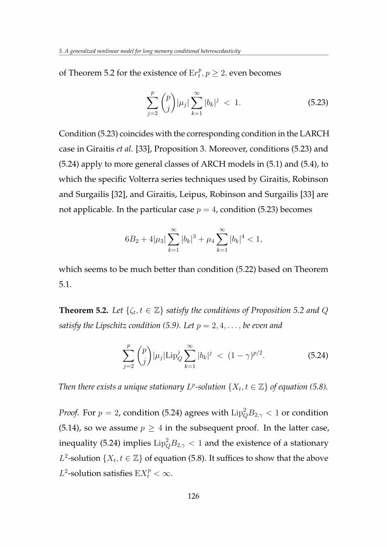
5. A generalized nonlinear model for long memory conditional heteroscedasticity

of Theorem 5.2 for the existence of Erpt , p ≥ 2, even becomes

p∑j=2

(p

j

)|µj|

∞∑k=1

|bk|j < 1. (5.23)

Condition (5.23) coincides with the corresponding condition in the LARCH

case in Giraitis et al. [33], Proposition 3. Moreover, conditions (5.23) and

(5.24) apply to more general classes of ARCH models in (5.1) and (5.4), to

which the specific Volterra series techniques used by Giraitis, Robinson

and Surgailis [32], and Giraitis, Leipus, Robinson and Surgailis [33] are

not applicable. In the particular case p = 4, condition (5.23) becomes

6B2 + 4|µ3|∞∑k=1

|bk|3 + µ4

∞∑k=1

|bk|4 < 1,

which seems to be much better than condition (5.22) based on Theorem

5.1.

Theorem 5.2. Let ζt, t ∈ Z satisfy the conditions of Proposition 5.2 and Q

satisfy the Lipschitz condition (5.9). Let p = 2, 4, . . . , be even and

p∑j=2

(p

j

)|µj|LipjQ

∞∑k=1

|bk|j < (1− γ)p/2. (5.24)

Then there exists a unique stationary Lp-solution Xt, t ∈ Z of equation (5.8).

Proof. For p = 2, condition (5.24) agrees with Lip2QB2,γ < 1 or condition

(5.14), so we assume p ≥ 4 in the subsequent proof. In the latter case,

inequality (5.24) implies Lip2QB2,γ < 1 and the existence of a stationary

L2-solution Xt, t ∈ Z of equation (5.8). It suffices to show that the above

L2-solution satisfies EXpt <∞.

126

5.2. Stationary solution

To this end, similarly as in the proof of Theorem 5.1 (i), consider the

solution X(n)t with zero initial condition at t ≤ −n as defined in (5.16).

Let σ(n)t := 0, t < −n. Since E(X

(n)t −Xt)

2 → 0 (n→∞), by Fatou’s lemma

it suffices to show that under condition (5.24)

E(X(n)t )p < C, (5.25)

where the constant C <∞ does not depend on t, n.

Since p is even, for any t > −n we have that

E(X(n)t )p =

t−1∑s1,...,sp=−n

E[bt−s1ζs1σ

(n)s1 · · · bt−spζspσ

(n)sp

]=

p∑j=2

(p

j

) t−1∑s=−n

bjt−sµjE[(σ(n)

s )j( s−1∑u=−n

bt−uζuσ(n)u

)p−j]. (5.26)

Hence using Hölder’s inequality:

|Eξjηp−j| ≤ cjEj/p|ξ/c|pE(p−j)/p|η|p

≤ cj[j

pcpE|ξ|p +

p− jp

E|η|p], 1 ≤ j ≤ p, c > 0,

we obtain

E(X(n)t )p ≤

p∑j=2

(p

j

)|µj|cj3

t−1∑s=−n

|bjt−s|j

pcp3E(σ(n)

s )p+

+p− jp

E

(s−1∑u=−n

bt−uζuσ(n)u

)p

=t−1∑s=−n

β1,t−sE(σ(n)s /c3)p +

t−1∑s=−n

β2,t−sE(X

(n)t,s

)p, (5.27)

127

5. A generalized nonlinear model for long memory conditional heteroscedasticity

where X(n)t,s :=

∑s−1u=−n bt−uζuσ

(n)u , c3 > LipQ, and where

β1,t−s :=

p∑j=2

j

p

(p

j

)|bjt−s||µj|c

j3, β2,t−s :=

p∑j=2

p− jp

(p

j

)|bjt−s||µj|c

j3.

The last expectation in (5.27) can be evaluated similarly to (5.26)–(5.27):

E(X

(n)t,s

)p=

p∑j=2

(p

j

) s−1∑u=−n

bjt−uµjE

(σ(n)u )j

(u−1∑v=−n

bt−vζvσ(n)v

)p−j≤

s−1∑u=−n

β1,t−uE(σ(n)u /c3)p +

s−1∑u=−n

β2,t−uE(X

(n)t,u

)p.

Proceeding recurrently with the above evaluation results in the inequality:

E(X(n)t )p ≤

t−1∑s=−n

βt−sE(σ(n)s /c3)p, (5.28)

where

βt−s := β1,t−s

(1 +

t−s−1∑k=1

∑s<uk<···<u1<t

β2,t−u1 · · · β2,t−uk

).

Let βi :=∑∞

t=1 βi,t, i = 1, 2, β :=∑∞

t=1 βt. By assumption (5.24),

β1 + β2 =

p∑j=2

(p

j

)|µj|cj3

∞∑k=1

|bk|j < (1− γ)p/2,

whenever σ3 − LipQ > 0 is small enough, and, therefore,

β

(1− γ)p/2≤ 1

(1− γ)p/2

∞∑t=1

β1,t

(1 +

∞∑k=1

βk2

)

=1

(1− γ)p/2β1

1− β2< 1. (5.29)

128

5.2. Stationary solution

Next, let us estimate the expectation on the r.h.s. of inequality (5.28) in

terms of expectations on the l.h.s. Using inequality (5.10) and Minkowski’s

inequalities, we obtain

E2/p(σ(n)s )p ≤

s+n∑`=0

γ`E2/p|Q(a+X(n)s−`|

p

≤s+n∑`=0

γ`E2/p|c21 + c2

2(a+X(n)s−`)

2|p/2

≤ C + c23

n+s∑`=0

γ`E2/p(X(n)s−`)

p,

where c3 > c2 > LipQ and c3 − LipQ > 0 can be arbitrarily small. Particu-

larly, for any fixed T ∈ Z,

sup−n≤s<T

E2/p(σ(n)s )p ≤ c2

3

(1− γ)sup

−n≤s<TE2/p(X(n)

s )p + C.

Substituting the last bound into inequality (5.28), we obtain

sup−n≤t<T

E2/p(X(n)t )p ≤ β2/p

(1− γ)sup

−n≤s<TE2/p(X(n)

s )p + C. (5.30)

Relations (5.30) and (5.29) imply

sup−n≤t<T

E2/p(X(n)t )p ≤ C

1− β2/p

(1−γ)

<∞

proving (5.25) as well as the theorem.

Example 5.1. (Asymmetric GARCH(1,1)). The asymmetric GARCH(1,1)

model of Engle [25] corresponds to

σ2t = c2 + (a+ brt−1)2 + γσ2

t−1, (5.31)

129

5. A generalized nonlinear model for long memory conditional heteroscedasticity

or

σ2t = θ + ψrt−1 + a11r

2t−1 + δσ2

t−1, (5.32)

in the parametrization of Sentana ([66], (5)), with parameters in equations

(5.31) and (5.32) related by

θ = c2 + a2, δ = γ, ψ = 2ab, a11 = b2. (5.33)

Under the condition that ζt = rt/σt are standardized i.i.d., a stationary

asymmetric GARCH(1,1) (or GQARCH(1,1) in the terminology of Sentana

[66]) process rt, t ∈ Z with finite variance and a 6= 0 exists if and only if

B2,γ = b2/(1− γ) < 1, or

b2 + γ < 1, (5.34)

see Theorem 5.1 (ii). Condition (5.34) agrees with condition a11 + δ < 1 for

covariance stationarity in Sentana [66]. Under the assumptions that the

distribution of ζt is symmetric and µ4 = Eζ4t <∞, Sentana [66] provides a

sufficient condition for finiteness of Er4t together with explicit formula

Er4t =

µ4θ[θ(1 + a11 + δ) + ψ2]

(1− a211µ4 − 2a11δ − δ2)(1− a11 − δ)

. (5.35)

The sufficient condition of Sentana [66] for Er4t <∞ is µ4a

211 + 2a11δ+ δ2 <

1, which translates to

µ4b4 + 2b2γ + γ2 < 1, (5.36)

in terms of the parameters of (5.31). Condition (5.36) seems weaker than

the sufficient condition µ4b4+6b2 < (1−γ)2 of Theorem 5.2 for the existence

130

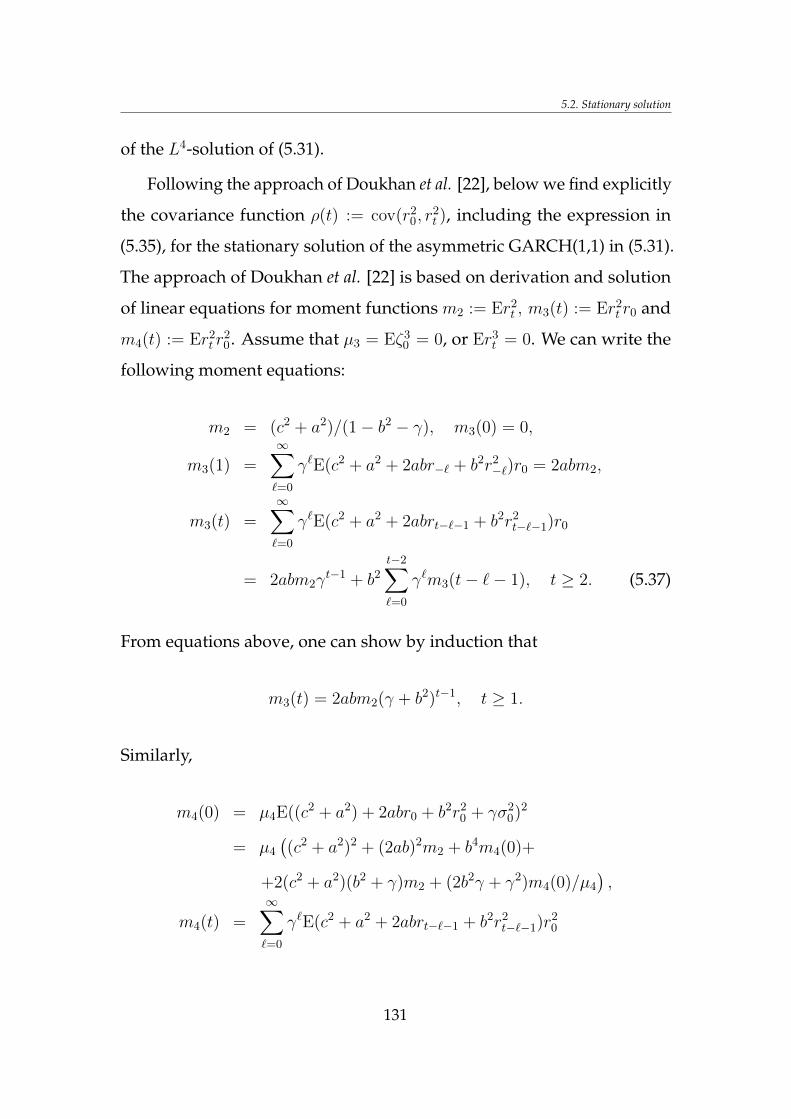
5.2. Stationary solution

of the L4-solution of (5.31).

Following the approach of Doukhan et al. [22], below we find explicitly

the covariance function ρ(t) := cov(r20, r

2t ), including the expression in

(5.35), for the stationary solution of the asymmetric GARCH(1,1) in (5.31).

The approach of Doukhan et al. [22] is based on derivation and solution

of linear equations for moment functions m2 := Er2t , m3(t) := Er2

t r0 and

m4(t) := Er2t r

20. Assume that µ3 = Eζ3

0 = 0, or Er3t = 0. We can write the

following moment equations:

m2 = (c2 + a2)/(1− b2 − γ), m3(0) = 0,

m3(1) =∞∑`=0

γ`E(c2 + a2 + 2abr−` + b2r2−`)r0 = 2abm2,

m3(t) =∞∑`=0

γ`E(c2 + a2 + 2abrt−`−1 + b2r2t−`−1)r0

= 2abm2γt−1 + b2

t−2∑`=0

γ`m3(t− `− 1), t ≥ 2. (5.37)

From equations above, one can show by induction that

m3(t) = 2abm2(γ + b2)t−1, t ≥ 1.

Similarly,

m4(0) = µ4E((c2 + a2) + 2abr0 + b2r20 + γσ2

0)2

= µ4

((c2 + a2)2 + (2ab)2m2 + b4m4(0)+

+2(c2 + a2)(b2 + γ)m2 + (2b2γ + γ2)m4(0)/µ4

),

m4(t) =∞∑`=0

γ`E(c2 + a2 + 2abrt−`−1 + b2r2t−`−1)r2

0

131

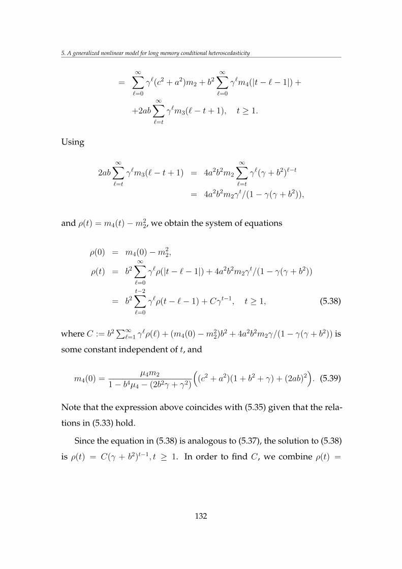
5. A generalized nonlinear model for long memory conditional heteroscedasticity

=∞∑`=0

γ`(c2 + a2)m2 + b2∞∑`=0

γ`m4(|t− `− 1|) +

+2ab∞∑`=t

γ`m3(`− t+ 1), t ≥ 1.

Using

2ab∞∑`=t

γ`m3(`− t+ 1) = 4a2b2m2

∞∑`=t

γ`(γ + b2)`−t

= 4a2b2m2γt/(1− γ(γ + b2)),

and ρ(t) = m4(t)−m22, we obtain the system of equations

ρ(0) = m4(0)−m22,

ρ(t) = b2∞∑`=0

γ`ρ(|t− `− 1|) + 4a2b2m2γt/(1− γ(γ + b2))

= b2t−2∑`=0

γ`ρ(t− `− 1) + Cγt−1, t ≥ 1, (5.38)

where C := b2∑∞

`=1 γ`ρ(`) + (m4(0)−m2

2)b2 + 4a2b2m2γ/(1− γ(γ + b2)) is

some constant independent of t, and

m4(0) =µ4m2

1− b4µ4 − (2b2γ + γ2)

((c2 + a2)(1 + b2 + γ) + (2ab)2

). (5.39)

Note that the expression above coincides with (5.35) given that the rela-

tions in (5.33) hold.

Since the equation in (5.38) is analogous to (5.37), the solution to (5.38)

is ρ(t) = C(γ + b2)t−1, t ≥ 1. In order to find C, we combine ρ(t) =

132

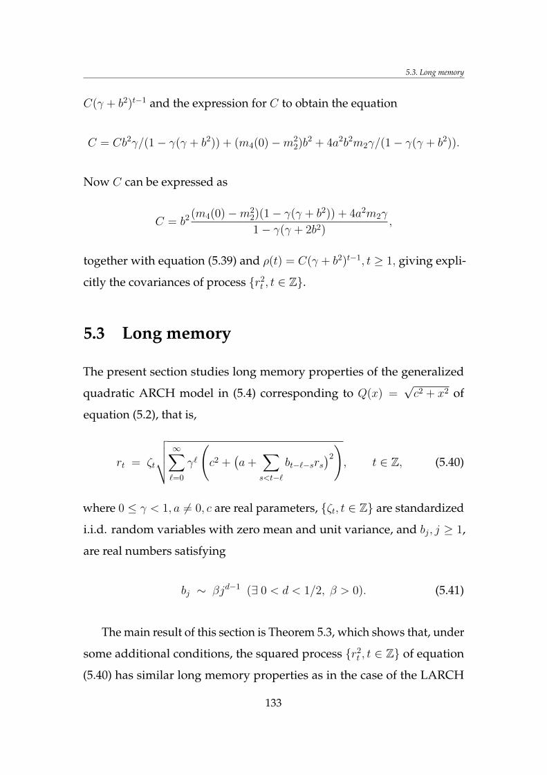
5.3. Long memory

C(γ + b2)t−1 and the expression for C to obtain the equation

C = Cb2γ/(1− γ(γ + b2)) + (m4(0)−m22)b2 + 4a2b2m2γ/(1− γ(γ + b2)).

Now C can be expressed as

C = b2 (m4(0)−m22)(1− γ(γ + b2)) + 4a2m2γ

1− γ(γ + 2b2),

together with equation (5.39) and ρ(t) = C(γ + b2)t−1, t ≥ 1, giving expli-

citly the covariances of process r2t , t ∈ Z.

5.3 Long memory

The present section studies long memory properties of the generalized

quadratic ARCH model in (5.4) corresponding to Q(x) =√c2 + x2 of

equation (5.2), that is,

rt = ζt

√√√√ ∞∑`=0

γ`

(c2 +

(a+

∑s<t−`

bt−`−srs)2

), t ∈ Z, (5.40)

where 0 ≤ γ < 1, a 6= 0, c are real parameters, ζt, t ∈ Z are standardized

i.i.d. random variables with zero mean and unit variance, and bj, j ≥ 1,

are real numbers satisfying

bj ∼ βjd−1 (∃ 0 < d < 1/2, β > 0). (5.41)

The main result of this section is Theorem 5.3, which shows that, under

some additional conditions, the squared process r2t , t ∈ Z of equation

(5.40) has similar long memory properties as in the case of the LARCH

133

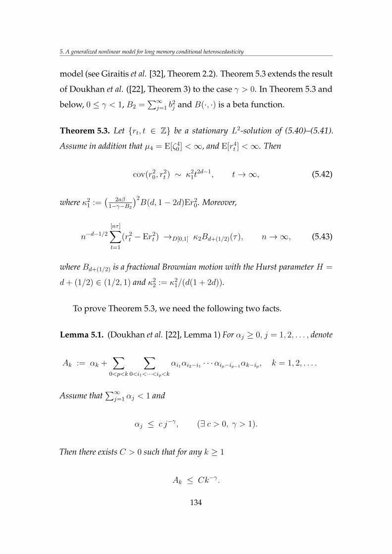
5. A generalized nonlinear model for long memory conditional heteroscedasticity

model (see Giraitis et al. [32], Theorem 2.2). Theorem 5.3 extends the result

of Doukhan et al. ([22], Theorem 3) to the case γ > 0. In Theorem 5.3 and

below, 0 ≤ γ < 1, B2 =∑∞

j=1 b2j and B(·, ·) is a beta function.

Theorem 5.3. Let rt, t ∈ Z be a stationary L2-solution of (5.40)–(5.41).

Assume in addition that µ4 = E[ζ40 ] <∞, and E[r4

t ] <∞. Then

cov(r20, r

2t ) ∼ κ2

1t2d−1, t→∞, (5.42)

where κ21 :=

(2aβ

1−γ−B2

)2B(d, 1− 2d)Er2

0. Moreover,

n−d−1/2

[nτ ]∑t=1

(r2t − Er2

t ) →D[0,1] κ2Bd+(1/2)(τ), n→∞, (5.43)

where Bd+(1/2) is a fractional Brownian motion with the Hurst parameter H =

d+ (1/2) ∈ (1/2, 1) and κ22 := κ2

1/(d(1 + 2d)).

To prove Theorem 5.3, we need the following two facts.

Lemma 5.1. (Doukhan et al. [22], Lemma 1) For αj ≥ 0, j = 1, 2, . . . , denote

Ak := αk +∑

0<p<k

∑0<i1<···<ip<k

αi1αi2−i1 · · ·αip−ip−1αk−ip, k = 1, 2, . . . .

Assume that∑∞

j=1 αj < 1 and

αj ≤ c j−γ, (∃ c > 0, γ > 1).

Then there exists C > 0 such that for any k ≥ 1

Ak ≤ Ck−γ.

134

5.3. Long memory

Lemma 5.2. Assume that 0 ≤ β < 1 and αj ∼ cj−γ (∃ γ > 0, c > 0). Then

αt,β :=t−1∑j=0

βjαt−j ∼c

1− βt−γ, t→∞.

Proof. It suffices to show that the difference Dt := αt,β − αt/(1− β) decays

faster than αt, in other words, that

Dt =t−1∑j=0

βj(αt − αt−j)−∞∑j=t

βjαt−j = o(t−γ).

Clearly,∑

t/2<j<t βj(αt−αt−j) = O(βt/2) = o(t−γ),

∑∞j=t β

jαt−j = O(βt) =

o(t−γ). Relation∑

0≤j≤t/2 βj(αt − αt−j) = o(t−γ) follows by the dominated

convergence theorem since sup0≤j≤t/2 |αt−αt−j|tγ ≤ C and |αt−αt−j|tγ →

0 for any fixed j ≥ 0.

Proof of Theorem 5.3. We use the idea of the proof of Theorem 3 by

Doukhan et al. [22]. Denote

bt,γ :=t−1∑j=0

γjbt−j, b2t,γ :=

t−1∑j=0

γjb2t−j, t ≥ 1, (5.44)

Xt :=∑s<t

bt−srs, Xt,γ :=∑s<t

bt−s,γrs, t ∈ Z.

By the definition of rt in (5.40), we have the following decomposition (c.f.

Doukhan et al. [22], (6.11))

(r2t − Er2

t )−∑s<t

b2t−s,γ(r

2s − Er2

s) = 2aXt,γ + Ut + Vt,γ =: ξt, (5.45)

where Xt,γ is the main term and the "remainder terms" Ut and Vt,γ are

135

5. A generalized nonlinear model for long memory conditional heteroscedasticity

given by

Ut := (ζ2t − Eζ2

t )σ2t , Vt,γ :=

∞∑`=0

γ`Vt−`, (5.46)

Vt := 2∑

s2<s1<t

bt−s1bt−s2rs1rs2. (5.47)

Using the identity Vt = (X2t −EX2

t )−∑

s<t b2t−2(r2

t −Er2t ), the convergence

in L2 of the series on the r.h.s. of equation (5.47) follows as in Doukhan et

al. [22] (6.12). Hence, the series for Vt,γ in (5.46) also converges in L2.

Let us prove that

cov(ξ0, ξt) ∼ 4a2cov(X0,γ, Xt,γ) ∼ 4a2λ21t

2d−1, t→∞, (5.48)

where λ21 = β2/(1− γ)2B(d, 1− 2d). The second relation in (5.48) follows

from bt,γ ∼ (β/(1−γ))td−1, t→∞, see Lemma 5.1, and the fact that Xt,γ =∑s<t bt−s,γrs is a moving average in stationary uncorrelated innovations

rs. Since Ut is also an uncorrelated sequence, cov(ξ0, Ut) = 0 (t ≥ 1),

and the first relation in (5.48) is a consequence of

E[U0Xt,γ] + E[U0Vt,γ] = o(t2d−1), (5.49)

E[X0,γVt,γ] + E[V0,γ(Xt,γ + Vt,γ)] = o(t2d−1). (5.50)

We have

E[U0Xt,γ] = bt,γE[U0r0] = O(td−1) = o(t2d−1)

and

E[U0Vt,γ] = 2bt,γDt = O(td−1) = o(t2d−1),

136

5.3. Long memory

where

|Dt| := |E[U0r0

∑s<0

bt−srs]| ≤ EU20 (Er4

0)1/2(E(∑s<0

bt−srs)4)1/2 ≤ C

follows from Rosenthal’s inequality in (5.11) since

E(∑s<0

bt−srs

)4

≤ K4Er40

(∑s<0

b2t−s

)2

≤ C.

This proves (5.49). The proof of (5.50) is analogous to that of Doukhan et

al. [22] (6.13)–(6.14) and is omitted.

Next, let us prove (5.42). Recall the definition of b2j,γ in (5.44). From the

decomposition (5.45), we obtain

r2t − Er2

t =∞∑i=0

φi,γξt−i, t ∈ Z, (5.51)

where φj,γ ≥ 0, j ≥ 0, are the coefficients of the power series

Φγ(z) :=∞∑j=0

φj,γzj = (1−

∞∑j=1

b2j,γz

j)−1, z ∈ C, |z| < 1,

given by φ0,γ := 1,

φj,γ := b2j,γ +

∑0<k<j

∑0<s1<···<sk<j

b2s1,γ · · · b

2sk−sk−1,γ b

2j−sk,γ, j ≥ 1.

From (5.41) and Lemmas 5.1 and 5.2, we infer that

φt,γ = O(t2d−2), t→∞, (5.52)

in particular, Φγ(1) =∑∞

t=0 φt,γ = (1− γ)/(1− γ −B2) <∞ and the r.h.s.

137

5. A generalized nonlinear model for long memory conditional heteroscedasticity

of equation (5.51) is well defined. Relations (5.51) and (5.52) imply that

cov(r2t , r

20) =

∞∑i,j=0

φiφjcov(ξt−i, ξ−j) ∼ Φ2γ(1)cov(ξt, ξ0), t→∞, (5.53)

see Doukhan et al. [22], (6.20). Now, (5.42) follows from relations (5.53)

and (5.48). The invariance principle in (5.43) follows similarly as in the

proof of Theorem 3 by Doukhan et al. [22], from (5.51), (5.48) and

n−d−1/2

[nτ ]∑t=1

Xt,γ →D[0,1] λ2Wd+(1/2)(τ), λ22 = λ2

1/d(1 + 2d),

the last fact being a consequence of a general result of Abadir er al. [1].

Theorem 5.3 is proved.

5.4 Leverage

For the conditionally heteroscedastic model in (5.40) with Eζt = Eζ3t =

0,Eζ2t = 1, consider the leverage function ht = cov(σ2

t , r0) = Er2t r0, t ≥ 1.

Following Giraitis et al. [33], and Doukhan et al. [22], we say that rt, t ∈

Z, in equation (5.40) has leverage of order k ≥ 1 (denoted by rt ∈ `(k)) if

hj < 0, 1 ≤ j ≤ k.

The study by Doukhan et al. [22] of leverage for model (5.40) with γ = 0,

that is,

rt = ζt

√√√√c2 +

(a+

∑s<t

bt−srs

)2

, t ∈ Z,

138

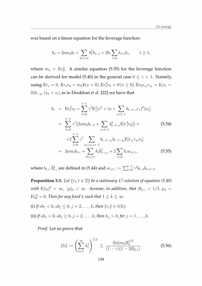
5.4. Leverage

was based on a linear equation for the leverage function:

ht = 2am2bt +∑

0<i<t

b2iht−i + 2bt

∑i>0

bi+thi, t ≥ 1,

where m2 = Er20. A similar equation (5.55) for the leverage function

can be derived for model (5.40) in the general case 0 ≤ γ < 1. Namely,

using Ers = 0, Ersr0 = m21(s = 0),Er2sr0 = 0 (s ≤ 0),Er0rs1rs2 = 1(s1 =

0)h−s2 (s2 < s1) as in Doukhan et al. [22] we have that

ht = Er2t r0 =

t−1∑`=0

γ`E[(c2 + (a+

∑s<t−`

bt−`−srs)2)r0

]=

t−1∑`=0

γ`(2am2bt−` +

∑s<t−`

b2t−`−sE[r2

sr0])

+ (5.54)

+2t−1∑`=0

γ`∑

s2<s1<t−`

bt−`−s1bt−`−s2E[rs1rs2r0]

= 2am2bt,γ +∑

0<i<t

hib2t−i,γ + 2

∑i>0

hiwi,t,γ, (5.55)

where bt,γ, b2t,γ are defined in (5.44) and wi,t,γ :=

∑t−1`=0 γ

`bt−`bi+t−`.

Proposition 5.3. Let rt, t ∈ Z be a stationary L2-solution of equation (5.40)

with E|r0|3 < ∞, |µ|3 < ∞. Assume, in addition, that B2,γ < 1/5, µ3 =

Eζ30 = 0. Then for any fixed k such that 1 ≤ k ≤ ∞:

(i) if ab1 < 0, abj ≤ 0, j = 2, . . . , k, then rt ∈ `(k);

(ii) if ab1 > 0, abj ≥ 0, j = 2, . . . , k, then hj > 0, for j = 1, . . . , k.

Proof. Let us prove that

‖h‖ :=

( ∞∑t=1

h2t

)1/2

≤ 2|a|m2B1/22

(1− γ)(1− 3B2,γ). (5.56)

139

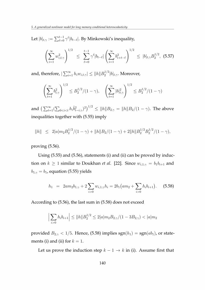
5. A generalized nonlinear model for long memory conditional heteroscedasticity

Let |b|t,γ :=∑t−1

`=0 γ`|bt−`|. By Minkowski’s inequality,

( ∞∑i=1

w2i,t,γ

)1/2

≤t−1∑`=0

γ`|bt−`|

( ∞∑i=1

b2i+t−`

)1/2

≤ |b|t,γB1/22 , (5.57)

and, therefore, |∑∞

i=1 hiwi,t,γ| ≤ ‖h‖B1/22 |b|t,γ . Moreover,

( ∞∑t=1

b2t,γ

)1/2

≤ B1/22 /(1− γ),

( ∞∑t=1

|b|2t,γ

)1/2

≤ B1/22 /(1− γ)

and(∑∞

t=1(∑

0<i<t hib2t−i,γ)

2)1/2 ≤ ‖h‖B2,γ = ‖h‖B2/(1 − γ). The above

inequalities together with (5.55) imply

‖h‖ ≤ 2|a|m2B1/22 /(1− γ) + ‖h‖B2/(1− γ) + 2‖h‖B1/2

2 B1/22 /(1− γ),

proving (5.56).

Using (5.55) and (5.56), statements (i) and (ii) can be proved by induc-

tion on k ≥ 1 similar to Doukhan et al. [22]. Since wi,1,γ = b1bi+1 and

b1,γ = b1, equation (5.55) yields

h1 = 2am2b1,γ + 2∑i>0

wi,1,γhi = 2b1

(am2 +

∑i>0

hibi+1

). (5.58)

According to (5.56), the last sum in (5.58) does not exceed

∣∣∣∑i>0

hibi+1

∣∣∣ ≤ ‖h‖B1/22 ≤ 2|a|m2B2,γ/(1− 3B2,γ) < |a|m2

provided B2,γ < 1/5. Hence, (5.58) implies sgn(h1) = sgn(ab1), or state-

ments (i) and (ii) for k = 1.

Let us prove the induction step k − 1 → k in (i). Assume first that

140

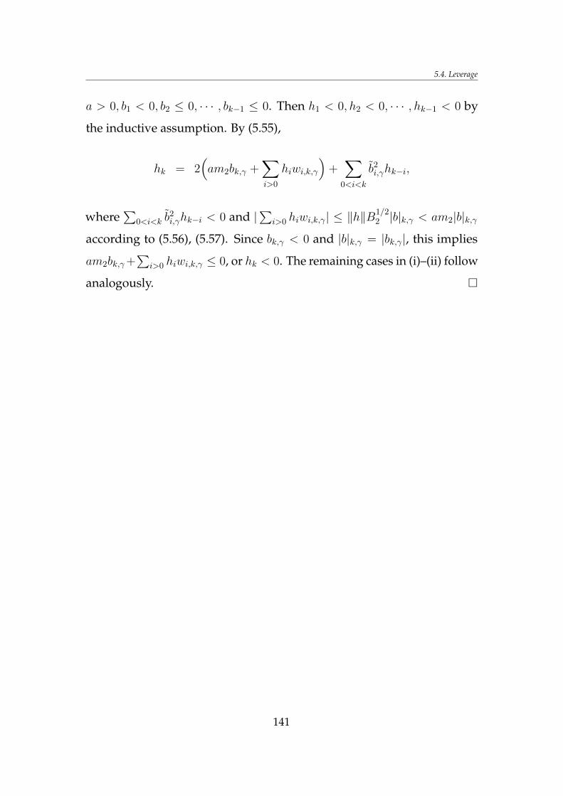
5.4. Leverage

a > 0, b1 < 0, b2 ≤ 0, · · · , bk−1 ≤ 0. Then h1 < 0, h2 < 0, · · · , hk−1 < 0 by

the inductive assumption. By (5.55),

hk = 2(am2bk,γ +

∑i>0

hiwi,k,γ

)+∑

0<i<k

b2i,γhk−i,

where∑

0<i<k b2i,γhk−i < 0 and |

∑i>0 hiwi,k,γ| ≤ ‖h‖B

1/22 |b|k,γ < am2|b|k,γ

according to (5.56), (5.57). Since bk,γ < 0 and |b|k,γ = |bk,γ|, this implies

am2bk,γ+∑

i>0 hiwi,k,γ ≤ 0, or hk < 0. The remaining cases in (i)–(ii) follow

analogously.

141

Chapter 6

Conclusions

In this last chapter, we summarize the main results of the dissertation:

• in this dissertation we showed that FIGARCH and IARCH(∞) equa-

tions with zero intercept may have a nontrivial covariance stationary

solution with long memory;

• we provided a complete answer to the long standing conjecture

of Ding and Granger ([20], 1996) about the existence of the Long

Memory ARCH model;

• we introduced and investigated a new class of long memory integ-

rated AR(p, d, q) processes and showed that their autocovariance can

be modeled easily at low lags without a significant effect on the

long memory behavior, this being a major advantage over classical

ARFIMA models;

• we also obtained necessary and sufficient conditions for the existence

of stationary integrated AR(∞) processes with finite variance and

proved that such processes always have long memory;

142

• we studied the five-parametric QML estimation for a quadratic

ARCH process with long memory and strictly positive conditional

variance. Several QML estimators of unknown parameter θ0 ∈ R5 of

our model were discussed, in particular, an estimator depending on

observations from the infinite past, and a class of estimators depend-

ing only on observations from the finite past. We proved consistency

and asymptotic normality of these estimators;

• a simulation study of the empirical MSE of QML estimation was

included. In the simulation experiment, we studied the empirical

performance of a more realistic version of the estimator and showed

that the empirical RMSEs of this estimator show a good agreement

with theoretical standard deviations;

• we studied the existence and properties of a stationary solution of

the ARCH-type equation rt = ζtσt, where the conditional variance

satisfies σ2t = Q2

(a+

∑∞j=1 bjrt−j

)+ γσ2

t−1 with a Lipschitz function

Q(x) and real parameters a, γ, bj . We obtained conditions for the

existence of a stationary solution, and, in particular, when Q is the

square root of a quadratic polynomial, we proved that rt can exhibit

a leverage effect and long memory.

143

Bibliography

[1] K. M. Abadir, W. Distaso, L. Giraitis, and H. L. Koul. Asymptotic

normality for weighted sums of linear processes. Econometric Theory,

30:252–284, 2014.

[2] B. D. O. Andersen and J. B. Moore. Optimal Filtering. Prentice Hall,

Inc., Englewood Cliffs, N.J., 1979.

[3] R. T. Baillie, T. Bollerslev, and H. O. Mikkelsen. Fractionally in-

tegrated generalized autoregressive conditional heteroscedasticity.

Journal of Econometrics, 74:3–30, 1996.

[4] J. Beran. Statistics for long-memory processes. Chapman and Hall, New

York, 1994.

[5] J. Beran and M. Schützner. On approximate pseudo-maximum like-

lihood estimation for LARCH-processes. Bernoulli, 15:1057–1081,

2009.

[6] I. Berkes and L. Horváth. The rate of consistency of the quasi-

maximum likelihood estimator. Statistics and Probability Letters, 61:

133–143, 2003.

[7] I. Berkes and L. Horváth. The efficiency of the estimators of the

parameters in GARCH processes. Annals of Statistics, 32:633–655,

2004.

[8] I. Berkes, L. Horváth, and P. S. Kokozska. GARCH processes: struc-

144

Bibliography

ture and estimation. Bernoulli, 9:201–227, 2003.

[9] P. Billingsley. Convergence of Probability Measures. New York: Wiley,

1968.

[10] T. Bollerslev. Generalized autoregressive conditional heteroskedasti-

city. Journal of Econometrics, 31:307–327, 1986.

[11] A. Bose and K. Mukherjee. Estimating the ARCH parameters by

solving linear equations. Journal of Time Series Analysis, 24:127–136,

2003.

[12] P. Bougerol and N. Picard. Stationarity of GARCH processes and

of some nonnegative time series. Journal of Econometrics, 52:115–127,

1992.

[13] P. J. Brockwell and R. A. Davis. Time Series: Theory and Methods (2nd

edition). Springer Series in Statistics. Springer-Verlag, New York.,

1991.

[14] DL. Burkholder. Distribution functions inequalities for martingales.

Annals of Probability, 1:19–42, 1973.

[15] V. Kazakevicius and R. Leipus. On stationarity in the ARCH(∞)

model. Econometric Theory, 18:1–16, 2002.

[16] V. Kazakevicius and R. Leipus. A new theorem on existence of

invariant distributions with applications to ARCH processes. Journal

of Applied Probability, 40:147–162, 2003.

[17] D. R. Cox. Long-range dependence: a review. In Statistics: An

Appraisal. Proc. 50th Anniversary Conference, pages 55–74. Iowa State

University Press, 2009.

[18] J. Davidson. Moment and memory properties of linear conditional

heteroscedasticity models, and a new model. Journal of Business and

Economic Statistics, 22:16–29, 2004.

145

Bibliography

[19] R. B. Davies and D. S. Harte. Tests for Hurst effect. Biometrica, 74:

95–102, 1987.

[20] Z. Ding and C. W. J. Granger. Modelling volatility persistence of

speculative returns: A new approach. Journal of Econometrics, 73:

185–215, 1996.

[21] R. Douc, F. Roueff, and P. Soulier. On the existence of some ARCH(∞)

processes. Stochastic Processes and their Applications, 118:755–761, 2008.

[22] P. Doukhan, I. Grublyte, and D. Surgailis. A nonlinear model for

long memory conditional heteroscedasticity. Lithuanian Mathematical

Journal, 56:164–188, 2016.

[23] A. Osekowski. A note on Burkholder-Rosenthal inequality. Bulletin

of the Polish Academy Sciencies. Mathematics, 60:177–185, 2012.

[24] R. F. Engle. Autoregressive conditional heteroscedasticity with estim-

ates of the variance of United Kingdom inflation. Econometrica, 50:

987–1008, 1982.

[25] R. F. Engle. Stock volatility and the crash of ’87. Discussion. The

Review of Financial Studies, 3:103–106, 1990.

[26] C. Francq and JM. Zakoian. Maximum likelihood estimation of pure

GARCH and ARMA-GARCH processes. Bernoulli, 10:605–637, 2004.

[27] C. Francq and JM. Zakoian. A tour in the asymptotic theory of

GARCH estimation. In Handbook of financial time series, pages 85–109.

Springer-Verlag Berlin Heidelberg, 2009.

[28] C. Francq and JM. Zakoian. GARCH models: Structure, Statistical

Inference and Financial Applications. New York: Wiley, 2010.

[29] C. Francq and JM. Zakoian. Inconsistency of the MLE and inference

based on weighted LS for LARCH models. Journal of Econometrics,

159:151–165, 2010.

146

Bibliography

[30] L. Giraitis and D. Surgailis. ARCH-type bilinear models with double

long memory. Stochastic Processes and their Applications, 100:275–300,

2002.

[31] L. Giraitis, P. Kokoszka, and R. Leipus. Stationary ARCH models:

dependence structure and central limit theorem. Econometric Theory,

16:3–22, 2000.

[32] L. Giraitis, P. M. Robinson, and D. Surgailis. A model for long

memory conditional heteroscedasticity. The Annals of Applied Probab-

ility, 10:1002–1024, 2000.

[33] L. Giraitis, R. Leipus, P. M. Robinson, and D. Surgailis. LARCH,

leverage and long memory. Journal of Financial Econometrics, 2:177–

210, 2004.

[34] L. Giraitis, R. Leipus, and D. Surgailis. Recent advances in ARCH

modelling. In Long Memory in Economics, pages 3–38. Springer-Verlag,

2007.

[35] L. Giraitis, R. Leipus, and D. Surgailis. ARCH(∞) models and long

memory properties. In Handbook of financial time series, pages 71–84.

Springer-Verlag Berlin Heidelberg, 2009.

[36] L. Giraitis, H. L. Koul, and D. Surgailis. Large sample inference for long

memory processes. Imperial College press, 2012. ISBN 978-1-84816-278-

5.

[37] L. Giraitis, D. Surgailis, and A. Škarnulis. Stationary integrated

ARCH(∞) and AR(∞) processes with finite variance. Under revision

in Econometric Theory, 2017.

[38] C. W. J. Granger and A. P. Andersen. An Introduction to Bilinear Time

Series Models. Vandenhoek and Ruprecht, Göttingen, 1978.

[39] C. W. J. Granger and Z. Ding. Some properties of absolute return: an

147

Bibliography

alternative measure of risk. Annales d’Economie et de Statistique, 40:

67–91, 1995.

[40] I. Grublyte and A. Škarnulis. A nonlinear model for long memory

conditional heteroscedasticity. Statistics, 51:123–140, 2017.

[41] I. Grublyte, D. Surgailis, and A. Škarnulis. QMLE for quadratic

ARCH model with long memory. Journal of Time Series Analysis, 2016.

doi: 10.1111/jtsa.12227.

[42] P. Hall and Q. Yao. Inference in ARCH and GARCH models with

heavy-tailed errors. Econometrica, 71:285–317, 2003.

[43] J. D. Hamilton. Time series analysis. Princeton University Press, Prin-

ceton, 1994.

[44] J. R. M. Hosking. Fractional differencing. Biometrika, 68:165–176,

1981.

[45] J. K. Hunter and B. Nachtergaele. Applied Analysis. World Scientific

Publishing Co.Pte. Ltd., 2001.

[46] H. Hurst. Long-term storage capacity of reservoirs. Transactions of

the American Society of Civil Engineers, 116:770–808, 1951.

[47] H. Hurst. Methods of using long-term storage in reservoirs. Proceed-

ings of the Institution of Civil Engineers, Part I, pages 519–577, 1955.

[48] I. A. Ibragimov and Yu. V. Linnik. Independent and Stationary Sequences

of Random Variables. Wolters-Noordhoff, Groningen, 1971.

[49] P. Kokoszka and R. Leipus. Change-point estimation in ARCH mod-

els. Bernoulli, 6:513–539, 2000.

[50] D. Koulikov. Long memory ARCH(∞) models: Specification and

quasi-maximum likelihood estimation. Working Paper 163, Centre for

Analytical Finance, Univ. Aarhus. www.cls.dk/caf/wp/wp-163.pdf, 2003.

[51] R. Leipus and V. Kazakevicius. On stationarity in the ARCH(∞)

148

Bibliography

model. Econometric Theory, 18:1–16, 2002.

[52] M. Levine, S. Torres, and F. Viens. Estimation for the long-memory

parameter in LARCH models, and fractional Brownian motion. Stat-

istical Inference for Stochastic Processes, 12:221–250, 2009.

[53] O. Lieberman and P. C. B. Phillips. Refined inference on long memory

in realized volatility. Econometric Reviews, 27:254–267, 2008.

[54] A.M. Lindner. Statioanrity, mixing, distributional properties and

moments of GARCH(p,q)-processes. In Handbook of financial time

series, pages 43–69. Springer-Verlag Berlin Heidelberg, 2009.

[55] B. Mandelbrot. Une classe de processus stochastiques homothetiques

a soi; application a loi climatologique de h. e. hurst. Comptes Rendus

Academic Sciences Paris, 240:3274–3277, 1965.

[56] B. Mandelbrot and J. Wallis. Noah, Joseph and operational hydrology.

Water Resources Research, 4:909–918, 1968.

[57] T. Mikosch and C. Starica. Is it really long memory we see in financial

returns? In Extremes and Integrated Risk Management, London, pages

149–168. Risk Books, 2000.

[58] T. Mikosch and C. Starica. Long-range dependence effects and ARCH

modeling. In Theory and Applications of Long-Range Dependence, pages

439–459. Birkhäuser, 2003.

[59] P. Moran. On the range of cumulative sums. Annals of the Institute of

Statistical Mathematics, 16:109–112, 1964.

[60] D. B. Nelson. Stationarity and persistence in the GARCH(1,1) model.

Econometric Theory, 6:318–334, 1990.

[61] T. Subba Rao. On the theory of bilinear time series models. Journal of

the Royal Statistical Society. Series B (Methodological), 43:244–255, 1981.

[62] P. M. Robinson. Testing for strong serial correlation and dynamic

149

Bibliography

conditional heteroskedasticity in multiple regression. Journal of Eco-

nometrics, 47:67–84, 1991.

[63] P. M. Robinson and P. Zaffaroni. Pseudo-maximum likelihood es-

timation of ARCH(∞) models. The Annals of Statistics, 34:1049–1074,

2006.

[64] HP. Rosenthal. On the subspaces of lp(p > 2) spanned by the se-

quences of independent random variables. Israel Journal of Mathemat-

ics, 8:273–303, 1970.

[65] W. Rudin. Real and Complex Analysis. McGraw-Hill Book Company,

New York etc., 1987.

[66] E. Sentana. Quadratic ARCH models. The Review of Economic Studies,

3:77–102, 1995.

[67] W. Stout. Almost sure convergence. New York: Academic Press, 1974.

[68] L. Truquet. On a family of contrasts for parametric inference in

degenerate ARCH models. Econometric Theory, 30:1165–1206, 2014.

[69] B. von Bahr and C-G. Esséen. Inequalities for the rth absolute moment

of a sum of random variables, 1 ≤ r ≤ 2. The Annals of Mathematical

Statistics, 36:299–303, 1965.

[70] P. Whittle. Estimation and information in stationary time series. Arkiv

för Matematik, 2:423–443, 1953.

150