Turku Centre for Computer Science

TUCS DissertationsNo 154, December 2012

Ville Rantala

On Dynamic Monitoring Methods for Networks-on-Chip

On Dynamic Monitoring Methods forNetworks-on-Chip

Ville Rantala

To be presented, with the permission of the Faculty of Mathematics and NaturalSciences of the University of Turku, for public criticism in Auditorium Lambda on

December 12, 2012, at 12 noon.

University of TurkuDepartment of Information Technology

20014 Turun yliopisto

2012

Supervisors

Adjunct Professor Juha PlosilaDepartment of Information TechnologyUniversity of Turku20014 Turun yliopistoFinland

Adjunct Professor Pasi LiljebergDepartment of Information TechnologyUniversity of Turku20014 Turun yliopistoFinland

Reviewers

Professor Gert JervanDepartment of Computer EngineeringTallinn University of TechnologyRaja 15, 12618 TallinnEstonia

Associate Professor Zhonghai LuDepartment of Electronic SystemsRoyal Institute of TechnologyForum 120, 16440 KistaSweden

Opponent

Professor Timo D. HamalainenDepartment of Computer SystemsTampere University of Technology33101 TampereFinland

ISBN 978-952-12-2822-3 (PRINT)ISBN 978-952-12-2823-0 (PDF)ISSN 1239-1883

Abstract

Rapid ongoing evolution of multiprocessors will lead to systems with hundreds of pro-cessing cores integrated in a single chip. An emerging challenge is the implementationof reliable and efficient interconnection between these cores as well as other componentsin the systems. Network-on-Chip is an interconnection approach which is intended tosolve the performance bottleneck caused by traditional, poorly scalable communicationstructures such as buses. However, a large on-chip network involves issues related tocongestion problems and system control, for instance. Additionally, faults can causeproblems in multiprocessor systems. These faults can be transient faults, permanentmanufacturing faults, or they can appear due to aging. To solve the emerging trafficmanagement, controllability issues and to maintain system operation regardless of faultsa monitoring system is needed. The monitoring system should be dynamically applicableto various purposes and it should fully cover the system under observation. In a largemultiprocessor the distances between components can be relatively long. Therefore,the system should be designed so that the amount of energy-inefficient long-distancecommunication is minimized.

This thesis presents a dynamically clustered distributed monitoring structure. Themonitoring is distributed so that no centralized control is required for basic tasks suchas traffic management and task mapping. To enable extensive analysis of differentNetwork-on-Chip architectures, an in-house SystemC based simulation environment wasimplemented. It allows transaction level analysis without time consuming circuit levelimplementations during early design phases of novel architectures and features.

The presented analysis shows that the dynamically clustered monitoring structurecan be efficiently utilized for traffic management in faulty and congested Network-on-Chip-based multiprocessor systems. The monitoring structure can be also successfullyapplied for task mapping purposes. Furthermore, the analysis shows that the presentedin-house simulation environment is flexible and practical tool for extensive Network-on-Chip architecture analysis.

i

ii

Acknowledgements

The research, presented in this thesis, was carried out during years 2008-2012 at theDepartment of Information Technology, University of Turku. The work was fundedby Academy of Finland and Turku Centre for Computer Science (TUCS) GraduateSchool, with financial support from the Nokia Foundation and the Finnish Foundationfor Technology Promotion. This thesis would not have been done without the supportfrom these organizations.

I would like to thank my supervisors Juha Plosila and Pasi Liljeberg for steering methrough this process which practically started in 2006 when I worked as a summer traineeat their laboratory. I wish to express my gratitude to Teijo Lehtonen for co-authoringseveral papers and guiding me through these years. I would also like to thank reviewersGert Jervan and Zhonghai Lu whose comments improved this thesis significantly. Ialso express my gratitude to professor Timo D. Hamalainen for agreeing to act as theopponent.

Warm thanks go also to the coffee room crews both at the Department of the Infor-mation Technology as well as at the Business Innovation Development Unit, especiallyto Sami Nuuttila for solving each and every computer related problem I was able todiscover.

Finally I would like to thank my parents Anne and Pasi for encouragement and sup-port towards whatever I have been doing.

Turku, November 5, 2012

Ville Rantala

iii

iv

Contents

1 Introduction 1

1.1 Objectives . . . . . . . . . . . . . . . . . . . . . . . . . . . . . . . . . . . . 2

1.2 Contributions . . . . . . . . . . . . . . . . . . . . . . . . . . . . . . . . . . 3

1.3 Publications . . . . . . . . . . . . . . . . . . . . . . . . . . . . . . . . . . . 3

1.4 Organization . . . . . . . . . . . . . . . . . . . . . . . . . . . . . . . . . . 4

2 Network-on-Chip 5

2.1 Components . . . . . . . . . . . . . . . . . . . . . . . . . . . . . . . . . . . 5

2.2 Topologies . . . . . . . . . . . . . . . . . . . . . . . . . . . . . . . . . . . . 7

2.2.1 Basic Topologies . . . . . . . . . . . . . . . . . . . . . . . . . . . . 8

2.2.2 Hierarchical Topologies . . . . . . . . . . . . . . . . . . . . . . . . 10

2.2.3 Irregular Topologies . . . . . . . . . . . . . . . . . . . . . . . . . . 10

2.3 Network Traffic Classification . . . . . . . . . . . . . . . . . . . . . . . . . 11

2.4 Network Flow Control . . . . . . . . . . . . . . . . . . . . . . . . . . . . . 11

2.5 Routing Algorithms . . . . . . . . . . . . . . . . . . . . . . . . . . . . . . 12

2.5.1 Deterministic Routing . . . . . . . . . . . . . . . . . . . . . . . . . 13

2.5.2 Stochastic Routing Algorithms . . . . . . . . . . . . . . . . . . . . 17

2.5.3 Adaptive Routing . . . . . . . . . . . . . . . . . . . . . . . . . . . 18

2.6 Network Problems . . . . . . . . . . . . . . . . . . . . . . . . . . . . . . . 20

2.7 Summary . . . . . . . . . . . . . . . . . . . . . . . . . . . . . . . . . . . . 21

3 Monitoring on Network-on-Chip 23

3.1 Purpose of Monitoring . . . . . . . . . . . . . . . . . . . . . . . . . . . . . 24

3.1.1 Traffic Management . . . . . . . . . . . . . . . . . . . . . . . . . . 24

3.1.2 Fault Detection . . . . . . . . . . . . . . . . . . . . . . . . . . . . . 25

3.1.3 Task Management . . . . . . . . . . . . . . . . . . . . . . . . . . . 25

3.2 Monitoring Structures . . . . . . . . . . . . . . . . . . . . . . . . . . . . . 26

3.2.1 Centralized Monitoring . . . . . . . . . . . . . . . . . . . . . . . . 27

3.2.2 Clustered Monitoring . . . . . . . . . . . . . . . . . . . . . . . . . 28

3.2.3 Localized Monitoring . . . . . . . . . . . . . . . . . . . . . . . . . . 29

3.2.4 Distributed Monitoring . . . . . . . . . . . . . . . . . . . . . . . . 30

3.3 Monitoring Trade-offs . . . . . . . . . . . . . . . . . . . . . . . . . . . . . 31

v

3.3.1 Resource Allocation . . . . . . . . . . . . . . . . . . . . . . . . . . 31

3.4 Fault Tolerance of Monitoring Systems . . . . . . . . . . . . . . . . . . . . 32

3.5 Summary . . . . . . . . . . . . . . . . . . . . . . . . . . . . . . . . . . . . 32

4 Dynamically Clustered Distributed Monitoring 33

4.1 Dynamically Clustered Monitoring Structure . . . . . . . . . . . . . . . . 33

4.2 Principles of Analysis . . . . . . . . . . . . . . . . . . . . . . . . . . . . . 36

4.3 Monitoring Traffic Overhead . . . . . . . . . . . . . . . . . . . . . . . . . . 37

4.4 Routing Algorithms . . . . . . . . . . . . . . . . . . . . . . . . . . . . . . 43

4.5 Monitoring Algorithms and Communication . . . . . . . . . . . . . . . . . 44

4.6 Summary . . . . . . . . . . . . . . . . . . . . . . . . . . . . . . . . . . . . 46

5 Simulation Environment 47

5.1 Architecture . . . . . . . . . . . . . . . . . . . . . . . . . . . . . . . . . . . 48

5.2 Architectural Components . . . . . . . . . . . . . . . . . . . . . . . . . . . 48

5.2.1 Router . . . . . . . . . . . . . . . . . . . . . . . . . . . . . . . . . . 48

5.2.2 Network Interface . . . . . . . . . . . . . . . . . . . . . . . . . . . 53

5.2.3 Link . . . . . . . . . . . . . . . . . . . . . . . . . . . . . . . . . . . 53

5.2.4 Core . . . . . . . . . . . . . . . . . . . . . . . . . . . . . . . . . . . 54

5.2.5 Monitor . . . . . . . . . . . . . . . . . . . . . . . . . . . . . . . . . 56

5.3 Simulator Components . . . . . . . . . . . . . . . . . . . . . . . . . . . . . 61

5.3.1 Packet . . . . . . . . . . . . . . . . . . . . . . . . . . . . . . . . . . 61

5.3.2 Terminator . . . . . . . . . . . . . . . . . . . . . . . . . . . . . . . 62

5.4 Simulator Functionality . . . . . . . . . . . . . . . . . . . . . . . . . . . . 62

5.4.1 Architecture . . . . . . . . . . . . . . . . . . . . . . . . . . . . . . 62

5.4.2 Top Level Control . . . . . . . . . . . . . . . . . . . . . . . . . . . 63

5.4.3 Traffic Pattern . . . . . . . . . . . . . . . . . . . . . . . . . . . . . 63

5.4.4 Fault Injection . . . . . . . . . . . . . . . . . . . . . . . . . . . . . 64

5.4.5 Task Mapping . . . . . . . . . . . . . . . . . . . . . . . . . . . . . 64

5.5 Summary . . . . . . . . . . . . . . . . . . . . . . . . . . . . . . . . . . . . 64

6 Traffic Management 65

6.1 Status Update Interval . . . . . . . . . . . . . . . . . . . . . . . . . . . . . 65

6.1.1 Status Update Interval Analysis . . . . . . . . . . . . . . . . . . . 67

6.1.2 Cost of Implementations . . . . . . . . . . . . . . . . . . . . . . . . 70

6.2 Status Data Diffusion . . . . . . . . . . . . . . . . . . . . . . . . . . . . . 72

6.2.1 Additional Status Data Processing . . . . . . . . . . . . . . . . . . 75

6.2.2 Status Data Diffusion Analysis . . . . . . . . . . . . . . . . . . . . 77

6.3 Format of Network Status Data . . . . . . . . . . . . . . . . . . . . . . . . 81

6.3.1 Granularity of the Router Status Values . . . . . . . . . . . . . . . 82

6.3.2 Combining Router and Link Statuses . . . . . . . . . . . . . . . . . 82

6.4 Serial Monitor Communication . . . . . . . . . . . . . . . . . . . . . . . . 86

6.5 Reduction of Monitors . . . . . . . . . . . . . . . . . . . . . . . . . . . . . 89

vi

6.6 Summary . . . . . . . . . . . . . . . . . . . . . . . . . . . . . . . . . . . . 91

7 Lightweight Task Mapping 937.1 Lightweight Distributed Task Mapping . . . . . . . . . . . . . . . . . . . . 94

7.1.1 Core Load Monitoring and Reporting . . . . . . . . . . . . . . . . 967.2 Mapping Decision Process . . . . . . . . . . . . . . . . . . . . . . . . . . . 96

7.2.1 Neighbor Evaluation . . . . . . . . . . . . . . . . . . . . . . . . . . 967.2.2 Mapping Decision Strategies . . . . . . . . . . . . . . . . . . . . . 99

7.3 Enhanced Monitoring System . . . . . . . . . . . . . . . . . . . . . . . . . 1007.4 Case Study: Mapping Tasks . . . . . . . . . . . . . . . . . . . . . . . . . . 1007.5 Summary and Future Work . . . . . . . . . . . . . . . . . . . . . . . . . . 104

8 Conclusions 107

vii

viii

List of Figures

2.1 Router . . . . . . . . . . . . . . . . . . . . . . . . . . . . . . . . . . . . . . 6

2.2 Basic components of a Network-on-Chip. . . . . . . . . . . . . . . . . . . . 7

2.3 Mesh network. . . . . . . . . . . . . . . . . . . . . . . . . . . . . . . . . . 8

2.4 Torus network. . . . . . . . . . . . . . . . . . . . . . . . . . . . . . . . . . 9

2.5 Fat-tree network. . . . . . . . . . . . . . . . . . . . . . . . . . . . . . . . . 9

2.6 Polygon network. . . . . . . . . . . . . . . . . . . . . . . . . . . . . . . . . 10

2.7 Star network. . . . . . . . . . . . . . . . . . . . . . . . . . . . . . . . . . . 10

2.8 Hierarchical hybrid mesh-ring network. . . . . . . . . . . . . . . . . . . . . 11

2.9 XY routing. . . . . . . . . . . . . . . . . . . . . . . . . . . . . . . . . . . . 14

2.10 Turn model routing algorithms. . . . . . . . . . . . . . . . . . . . . . . . . 15

2.11 Turnaround routing algorithm. . . . . . . . . . . . . . . . . . . . . . . . . 19

3.1 Network components and their connections. . . . . . . . . . . . . . . . . . 26

3.2 Clustered monitoring. . . . . . . . . . . . . . . . . . . . . . . . . . . . . . 29

3.3 Distributed monitoring. . . . . . . . . . . . . . . . . . . . . . . . . . . . . 30

4.1 Dynamic clusters. . . . . . . . . . . . . . . . . . . . . . . . . . . . . . . . . 35

4.2 Network topology in DCM structure. . . . . . . . . . . . . . . . . . . . . . 36

4.3 Number of transactions. . . . . . . . . . . . . . . . . . . . . . . . . . . . . 39

4.4 Maximum traverse lengths. . . . . . . . . . . . . . . . . . . . . . . . . . . 40

4.5 Distribution of monitoring traffic load in time. . . . . . . . . . . . . . . . 41

4.6 Routing directions. . . . . . . . . . . . . . . . . . . . . . . . . . . . . . . . 42

4.7 Routing direction in experimental routing algorithm. . . . . . . . . . . . . 43

4.8 Structure of monitoring packet payload. . . . . . . . . . . . . . . . . . . . 45

5.1 Structure of a 2x2 NoC. . . . . . . . . . . . . . . . . . . . . . . . . . . . . 49

5.2 Structure of a router. . . . . . . . . . . . . . . . . . . . . . . . . . . . . . . 50

5.3 Productive directions. . . . . . . . . . . . . . . . . . . . . . . . . . . . . . 51

5.4 Routing directions. . . . . . . . . . . . . . . . . . . . . . . . . . . . . . . . 52

5.5 Structure of a link. . . . . . . . . . . . . . . . . . . . . . . . . . . . . . . . 54

5.6 Structure of a core. . . . . . . . . . . . . . . . . . . . . . . . . . . . . . . . 55

5.7 Indexes of the neighbors. . . . . . . . . . . . . . . . . . . . . . . . . . . . . 57

5.8 Structure of a monitor. . . . . . . . . . . . . . . . . . . . . . . . . . . . . . 58

ix

6.1 Throughput: status update interval. . . . . . . . . . . . . . . . . . . . . . 666.2 Throughput: status update interval, 10% of the links are faulty. . . . . . . 676.3 Sent monitoring packets. . . . . . . . . . . . . . . . . . . . . . . . . . . . . 686.4 Sent monitoring packets, 10% of the links are faulty. . . . . . . . . . . . . 696.5 Diffusion of network status information. . . . . . . . . . . . . . . . . . . . 736.6 Diffusion of network status information as a function of time. . . . . . . . 756.7 Routing directions. . . . . . . . . . . . . . . . . . . . . . . . . . . . . . . . 766.8 Indexes of the neighbor routers. . . . . . . . . . . . . . . . . . . . . . . . . 776.9 Throughput: cluster size, additional status data processing. . . . . . . . . 786.10 Throughput: cluster size. . . . . . . . . . . . . . . . . . . . . . . . . . . . 796.11 Throughput: cluster size, additional status data processing, 10% of links

are faulty. . . . . . . . . . . . . . . . . . . . . . . . . . . . . . . . . . . . . 796.12 Throughput: cluster size, 10% of links are faulty. . . . . . . . . . . . . . . 806.13 Throughput: additional status data processing. . . . . . . . . . . . . . . . 816.14 Throughput: status granularity. . . . . . . . . . . . . . . . . . . . . . . . . 836.15 Throughput: status granularity, 10% of links are faulty. . . . . . . . . . . 836.16 Throughput: status granularity, additional status data processing. . . . . 846.17 Throughput: status granularity, additional status data processing, 10%

of links are faulty. . . . . . . . . . . . . . . . . . . . . . . . . . . . . . . . 846.18 Throughput: separate traffic and fault data and hybrid formats. . . . . . 856.19 Throughput: separate traffic and fault data and hybrid formats, 10% of

links are faulty. . . . . . . . . . . . . . . . . . . . . . . . . . . . . . . . . . 866.20 Throughput: serial communication. . . . . . . . . . . . . . . . . . . . . . . 876.21 Throughput: serial communication. . . . . . . . . . . . . . . . . . . . . . . 886.22 Patterns of removed monitors. . . . . . . . . . . . . . . . . . . . . . . . . . 896.23 Throughput: fewer monitors. . . . . . . . . . . . . . . . . . . . . . . . . . 906.24 Throughput: fewer monitors, 10% of links are faulty. . . . . . . . . . . . . 91

7.1 Mapping decision process. . . . . . . . . . . . . . . . . . . . . . . . . . . . 977.2 Task mapping initiator cores. . . . . . . . . . . . . . . . . . . . . . . . . . 1017.3 Core load with mapping decision strategy 1. . . . . . . . . . . . . . . . . . 1037.4 Core load with mapping decision strategy 2. . . . . . . . . . . . . . . . . . 1037.5 Core load with mapping decision strategy 3. . . . . . . . . . . . . . . . . . 1037.6 Core load with mapping decision strategy 4. . . . . . . . . . . . . . . . . . 103

x

List of Tables

6.1 Status update implementation complexity. . . . . . . . . . . . . . . . . . . 706.2 Monitoring system cost comparison. . . . . . . . . . . . . . . . . . . . . . 716.3 Cost of 100-router NoC with different monitoring structures. . . . . . . . 72

7.1 Neighbor evaluation approaches. . . . . . . . . . . . . . . . . . . . . . . . 1017.2 Task mapping results. . . . . . . . . . . . . . . . . . . . . . . . . . . . . . 102

xi

xii

List of Abbreviations

ALOAS Arbitration Look Ahead SchemeBE Best EffortDCM Dynamically Clustered MonitoringDyAD Dynamically Adaptive and DeterministicE EastFIFO First In, First OutFlit FLow control digIT or FLow control unITGS Guaranteed ServiceGT Guaranteed ThoughputI/O Input/OutputID IdentifierIP Intellectual PropertyIVAL Improved VALiant’s randomized algorithmMPSoC Multiprocessor System-on-ChipN NorthNI Network InterfaceNoC Network-On-ChipPE Processing ElementS SouthSoC System-On-ChipTDM Time Division MultiplexingTLM Transaction-Level ModelingTTL Time To LiveVHDL VHSIC Hardware Description LanguageVHSIC Very-High-Speed Integrated CircuitW West

xiii

xiv

Chapter 1

Introduction

Network-on-Chip (NoC ) is a promising interconnection paradigm for current and futurehigh-performance Systems-on-Chip (SoC ) [9, 16, 49]. These SoCs can include hundredsof separate processor cores, memories and other Intellectual Property (IP) blocks, andthe number of these components is increasing. Communication between these compo-nents is challenging. It can form a performance bottleneck, and therefore, largely de-termine the maximum performance and capacity of the whole system. Traditional SoCsutilize shared-medium, bus-based communication infrastructures. Bus-based structuresare adequate for a small number of components but are poorly scalable for larger sys-tems. When the number of components increases each component has less and lesscommunication capacity available, the shared-communication medium is able to handleonly one transaction at a time. The bus structure is poorly scalable and therefore notsuitable for high-performance multi-core or multiprocessor systems.

NoC is a nanoscale on-chip computer network which consists of routers and links.System components can be connected to the routers through network interfaces. On-chip networks can be constructed following different network topologies and they canutilize various routing algorithms to steer data from a source to a destination. The datacan be transferred in the form of data packets. The main advantages of a network-basedcommunication infrastructure are scalability and flexibility. The size of a system canbe increased without blocking the communication infrastructure, which is a problem intraditional bus-based communication infrastructures. Scaling the size of the network upincreases the network capacity and offers new additional communication paths while inbus-based structures up-scaling increases capacitance and rises possibility of congestion.

Two essential issues concerning high-performance NoCs are the congestion and fault-iness of the involved resources. Highly loaded computational resources can generate alarge amount of traffic which causes congestion to the network and in the worst caseblocks the network. A typical issue is unbalanced communication resource utilization.While part of network is highly loaded there can still be other resources in idle state.Network topologies and routing algorithms can be designed to minimize these issuesbut they are not able to balance network utilization without network monitoring and

1

monitoring-based reconfiguration. The monitoring is also essential to detect faults andreconfigure the system to operate despite such faults.

Manufacturing of complex multiprocessor systems requires utilization of modernnanoscale integrated circuit fabrication processes. These complex integrated circuitscan include manufacturing faults which prevent the utilization of components in thefaulty areas. Aging effects, for instance electromigration, can compose additional faultsto the system [62]. To improve system reliability and increase manufacturing yield thesecomplex systems should have mechanisms to maintain the functionality even thoughthere are faulty components in the system. These mechanisms should be able to detectinadequate functionality and reconfigure the system so that faulty parts can be isolatedand the overall functionality is maintained with a reasonable performance.

A monitoring system is an essential part of system reconfiguration in the cases ofhigh traffic load or faulty system conditions. It consists of probes and monitors andrequires dedicated or shared communication medium to move data between probes,monitors and other network components. A monitoring system collects various statusdata from the system and delivers the observed data to the components of the system.The collected data can be used to reconfigure system operation and that way maintainand improve the functionality of the system. The usage of a monitoring system is notlimited to avoidance and solving of traffic and fault related issues. The operation of alarge and complex multi-core or multiprocessor system requires extensive knowledge ofthe status of different components so that the operation of the system can be controlledand optimized. The monitoring system can be used for statistics collection or taskmapping purposes, for instance.

1.1 Objectives

The main objective of this work is to develop a scalable monitoring structure for high-performance NoC based multiprocessor systems which makes it possible to maintain sys-tem functionality under high computational and communication load and even thoughthere are faulty components in the system. The monitoring system should collect thestatus information from the system and deliver it as widely as necessary to ensure systemfunctionality. A goal is to implement the system as far as possible without centralizedcontrol so that maximal scalability and architectural fault tolerance can be obtained. Ar-chitectural fault tolerance refers to system architecture where faulty components havelocal influence on the functionality of a system but do not distract the overall functional-ity which is typically the case when a centralized controller becomes faulty. In a faultlessnetwork the maximal performance requires the balanced utilization of network resources.Therefore, the communication infrastructure should be able to monitor the network loadand direct the traffic also through less loaded areas. Balanced resource utilization alsobalances the energy consumption and, furthermore, equalizes the heat dissipation. En-ergy consumption and heat dissipation are both essential issues in modern integratedcircuits. Additionally, the Network-on-Chip monitoring system should be applicable for

2

system control purposes which include for instance task mapping methods.To enable extensive analysis of Networks-on-Chip a simulation environment is needed.

The simulator should operate on the transaction level without in-detail circuit-level im-plementations so that new ideas and approaches can be easily analyzed without timeconsuming circuit implementations. This simulation environment should be able tomodel large NoCs with different routing algorithms and monitoring structures.

1.2 Contributions

The main contributions of the thesis include:

• Dynamically clustered distributed monitoring structure which is scalable, flexibleand where the monitoring infrastructure is evenly distributed over the monitoredsystem. The dynamically clustered structure is presented in Chapter 4.

• SystemC based Network-on-Chip simulation environment which enables transac-tion level analysis of different Network-on-Chip architectures and their features.The simulation environment is presented in Chapter 5.

• Analysis of traffic management related features of the dynamically clustered mon-itoring structure. The analysis is studied in Chapter 6.

• Lightweight distributed task mapping method which is based on the dynamicallyclustered monitoring structure and where the cores are able to carry out taskmapping autonomously without complete knowledge of the system status. Thelightweight task mapping method is presented and studied in Chapter 7.

1.3 Publications

The results, presented in this thesis, are partly published previously in journal articles

• V. Rantala, P. Liljeberg and J. Plosila. Status Data and Communication Aspectsin Dynamically Clustered Network-on-Chip Monitoring. In Journal of Electricaland Computer Engineering, 2012(2012), 2012.

• V. Rantala, T. Lehtonen, P. Liljeberg and J. Plosila. Analysis of Monitoring Struc-tures for Network-on-Chip: a Distributed Approach. IGI International Journal ofEmbedded and Real-Time Communication Systems (IJERTCS), 2(1):49–67, 2011.

and conference articles

• V. Rantala, T. Lehtonen, P. Liljeberg and J. Plosila. Analysis of Status Data Up-date in Dynamically Clustered Network-on-Chip Monitoring. In 1st InternationalConference on Pervasive and Embedded Computing and Communication Systems,PECCS 2011, March 2011.

3

• V. Rantala, T. Lehtonen, P. Liljeberg and J. Plosila. Multi Network InterfaceArchitectures for Fault Tolerant Network-on-Chip. In International Symposiumon Signals, Circuits and Systems (ISSCS ’09), July 2009.

The results and discussion presented in Chapter 7 are new and they have not beenpublished previously.

1.4 Organization

The thesis is organized as follows. The basics of Networks-on-Chip are presented in Chap-ter 2. It includes the descriptions of NoC components and topologies as well as presentstypical problems regarding Networks-on-Chip. Monitoring is discussed in Chapter 3, in-cluding different monitoring structures and the purposes of monitoring. A dynamicallyclustered distributed monitoring approach for Networks-on-Chip is presented in Chapter4. The chapter includes the concept level analysis of the dynamically clustered moni-toring approach and discussion concerning routing and monitoring algorithms. Chapter5 presents SystemC based transaction level Network-on-Chip simulation environmentwhich is used to simulate and analyze the presented monitoring approach in chaptersto follow. Issues concerning traffic management using dynamically clustered monitor-ing are presented and analyzed in Chapter 6. In Chapter 7 the dynamically clusteredmonitoring is applied for task mapping purposes. Issues related to task mapping us-ing the presented monitoring system are discussed and the task mapping functionalitydemonstrated. Finally, conclusions are drawn and future work discussed in Chapter 8.

4

Chapter 2

Network-on-Chip

Network-on-Chip (NoC ) is an approach to implement the interconnection of large andcomplex integrated circuits. Principles of Networks-on-Chip are basically similar to prin-ciples of any computer network. The main components are similar with the componentsof computer networks but implemented in nanoscale. Topology of the network deter-mines how the components are organized and connected to each other. A significantpart of a network implementation is a routing algorithm which defines along which pathdata are transferred from a source to a destination.

Typically, in Network-on-Chip data are transferred in packets. Each packet includesa header and a payload. The actual data are stored as a payload while the headerincludes important control information. The most important part of data in the headeris an address of a destination but it can also include for instance an address of a sender,packet ID and some statistical data. Network flow control is a protocol which determineshow individual packets are moved in the network. Besides these, types of the networktraffic and basic problems are discussed in this chapter.

2.1 Components

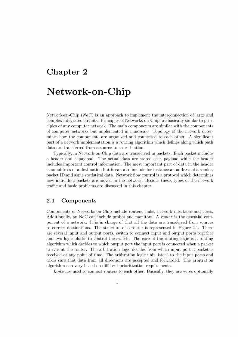
Components of Networks-on-Chip include routers, links, network interfaces and cores.Additionally, an NoC can include probes and monitors. A router is the essential com-ponent of a network. It is in charge of that all the data are transferred from sourcesto correct destinations. The structure of a router is represented in Figure 2.1. Thereare several input and output ports, switch to connect input and output ports togetherand two logic blocks to control the switch. The core of the routing logic is a routingalgorithm which decides to which output port the input port is connected when a packetarrives at the router. The arbitration logic decides from which input port a packet isreceived at any point of time. The arbitration logic unit listens to the input ports andtakes care that data from all directions are accepted and forwarded. The arbitrationalgorithm can vary based on different prioritization requirements.

Links are used to connect routers to each other. Basically, they are wires optionally

5

ZZ��

ZZ��Z

Z�� Z

Z�� Z

Z��Z

Z��

ZZ��Z

Z�� Z

Z�� Z

Z��

Input Ports

Output Ports

RoutingCrossbar Switch

ArbitrationLogic Logic

Figure 2.1: 5-port router.

with data buffering capabilities. If a transfer distance is relatively long, a link can haverepeaters to amplify the transferred signal. Buffer registers, where packets are storedwhile waiting for transferring forward, are implemented in links or in routers.

The purpose of a Network-on-Chip is to connect the components of an integratedcircuit to each other. These components are in this thesis called as cores. These com-ponents can be processors, memories or any intellectual property (IP) blocks.

In networks data are transferred in packets so the packets have to be generated beforethe data are sent to the network and also the packets have to be opened when they havebeen received from the network. These two operations are done in a network interface(NI ) which, as its name indicates, is an interface between a core and a network. Anetwork interface can be implemented as a part of a core and the core is able to connectto an interconnection network through it.

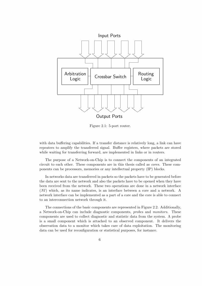
The connections of the basic components are represented in Figure 2.2. Additionally,a Network-on-Chip can include diagnostic components, probes and monitors. Thesecomponents are used to collect diagnostic and statistic data from the system. A probeis a small component which is attached to an observed component. It delivers theobservation data to a monitor which takes care of data exploitation. The monitoringdata can be used for reconfiguration or statistical purposes, for instance.

6

NI

Core

NI

Core

R R

@@ @@LinkLink

Link

Link

Figure 2.2: Basic components of a Network-on-Chip: router (R), link, core and networkinterface (NI) in a corner of a larger network.

2.2 Topologies

Topology defines the structure of a network. Interconnection networks can be catego-rized into four classes based on the network topology. These classes are shared-mediumnetworks, direct networks, indirect networks and hybrid networks. In the shared-mediumnetworks the transmission medium is shared by all components of the system. A busis an example of a shared-medium network. Each device connected to the bus has acertain time slot when it is allowed to use the bus and only one component can use theshared medium at a time. Arbitration logic is used to control who is able to use the busand for what duration. The major drawback of a shared-medium network is its lack ofscalability. When new components are connected to a bus, the time slot for each com-ponent has to be shortened and that way the communication performance most likelydecreases.

Direct networks are also known as point-to-point networks. In a direct networkeach component is directly connected to all the components it is communicating with.Therefore, any two components are not able to communicate with each other if they donot have a direct connection between each other. Shared-resource and direct networksare typically circuit switched networks which means that data are transferred withoutdividing it into packets. [51]

In a packet switched network, the raw data are divided into packets which are trans-ferred in the network individually. Packet switched communication is utilized in indirectnetworks. An indirect network consists of routers which compose a direct network be-tween them. Devices of the system are connected to routers through a network interface.[18] A hybrid network is a network which consists of a combination of different kinds ofnetworks.

A network is non-blocking if it is able to fulfill all the requests that are offered to it.In a packet switched networks, this kind of network is also called as a non-interferingnetwork. A non-interfering network can deliver all the packets in guaranteed time. [14]A basic network topology has one hierarchy layer where all the nodes are equal. Animproved version of this network topology is a hierarchical network where a network is

7

R R R R

R

R

RRRR

R

R R

R R

R

Figure 2.3: Mesh network.

divided into multiple hierarchy layers. Networks on the lower layer are called as thesubnetworks of a higher layer.

2.2.1 Basic Topologies

Mesh and Torus Probably the most utilized Network-on-Chip topology is mesh,presented in Figure 2.3. A mesh network consists of m columns and n rows. In themesh network, presented inf Figure 2.3, both m and n are four. The routers are locatedin the intersections of rows and column. Addresses of routers and resources can beeasily defined as X- and Y-coordinates of a mesh. The strength of the mesh network isits simplicity. It can be easily placed on a chip without complicated routing of wires.However, weakness of a mesh topology is varying distance between routers. Averagedistance from center of a network is shorter than from routers at the edges of mesh. [14]

A torus network is an improved version of the basic mesh network. A simple torusnetwork is a mesh where the heads of the columns are connected to the tails of thecolumns and the left sides of the rows are connected to the right sides of the rows. Atorus network has better path diversity than a mesh network, which means that thereare more alternative routes between two nodes of the network. The average distancebetween routers is constant on the contrary to the mesh. A torus network is shown inFigure 2.4. The chip implementation of a torus network is more complicated than themesh network due to the links from an edge to another edge. These links can also requiresignal repeaters due to their relatively long length. [38]

Tree and Butterfly Topologies In a tree network routers are placed at differentlevels and cores are connected to the routers on the lowest level [11]. The routers onhigher levels are called as ancestors of the routers below them. A fat-tree topology isillustrated in Figure 2.5. The cores can be connected to four routers at the bottom of thefigure. In the fat-tree topology, the routers are connected to multiple ancestors whichincreases the path diversity in the network and offers multiple routes between cores.

A butterfly network is a duplicated tree network. It consists of two tree networks

8

� �� �� �� �

��

��

��

��R R R R

R

R

RRRR

R

R R R

RR

Figure 2.4: Torus network.

from which another is turned around and connected above the original tree network.This way cores can be connected not only to the routers at the bottom of the networkbut also to the routers on the top of the network. The highest ancestor routers are inthe middle of the network. [28]

Polygon and Star Topologies The simplest polygon network is a circular networkwhere packets travel in a loop from a router to another in uni- or bidirectional path.Network becomes more diverse when chords are added to the circle. A polygon networkis fully connected if there is a direct link from every router to every other router in thenetwork. A fully connected polygon network is presented in Figure 2.6.

A star network, which is represented in Figure 2.7, is another simple network topol-ogy. It consists of a central router in the middle of the star, and cores in the spikes ofthe star. The capacity requirements of the central router are quite large, because allthe traffic between the spikes goes through the central router. That causes a remarkablepossibility of congestion in the middle of the star.[60]

������

�����

���

���

������

@@@

@@@

HHH

HHHHH

HHH

@@@

@@@

R R

R RRR

Figure 2.5: Fat-tree network.

9

����������

AAAAAAAAAA

�����

AAAAA

HHH

HHH

HH

����

����

�����

TTTTT

���

���

��

HHHH

HHHH

R R

RR

R R

Figure 2.6: Fully connected polygon (hexagon) network.

2.2.2 Hierarchical Topologies

Hierarchical topologies are based on an idea that multiple networks are connected to eachother with an upper level network, a global network. The originally separate networks,or subnetworks, are also called as the clusters of the network. This approach is useful insituations where most of the traffic is between components in a cluster but there is stilla need to have a connection to the components located in the other clusters.

A hierarchical hybrid topology is a combination of two different network topologies.Subnetworks have different topology than the global network. A hierarchical hybridnetwork with local mesh networks and a global polygon network is represented in Figure2.8.

2.2.3 Irregular Topologies

Irregular networks do not follow any regular topology. An irregular network has anapplication specific structure where routers are connected to the cores and to each otherbased on a known traffic pattern. Only the communication paths, which are required bythe application, are implemented.

TTT

���

���

TTT

R

RR

R

R

R

R

Figure 2.7: Star network.

10

RR R R R R

RR R R R R

RR R R R R

RR R R R R

RR R R R R

RR R R R R

Figure 2.8: Hierarchical hybrid network with a global ring topology and local meshtopologies.

2.3 Network Traffic Classification

The traffic in Networks-on-Chip may be classified into two categories: guaranteed through-put (GT) traffic and best effort (BE) traffic. Guaranteed throughput is also called asguaranteed service (GS). When guaranteed throughput is utilized the specification of thesystem guarantees that some defined portion of sent data reach its destination in a giventime frame. Guaranteed throughput works best with a routing algorithm that operatessimilarly as a circuit switched network, which means that the packets are sent from asender to a receiver through a fixed path and this path is not used by other senders atthe same time. All interference has to be minimized on the used path.

Best effort packets are transferred as trustworthy as possible. There are still noguarantees that best effort packets will ever reach the receiver. Latencies can vary andin the worst case packets can be lost for instance due to un-delivered packet removalmechanisms. Traffic in a basic packet switched network is mostly best effort traffic.In a packet switched network packets from a sender to a receiver may not move alongthe same path especially when adaptive routing algorithms are used (see Section 2.5.3).The packets from different senders move simultaneously in the network and share thenetwork resources. [14] Therefore, fixed performance cannot be guaranteed but thenetwork performance depends on the contemporary traffic pattern.

2.4 Network Flow Control

Network flow control determines how packets are transmitted inside a network. The flowcontrol is not directly dependent on a routing algorithm so that usage of a certain routingalgorithm does not necessarily require utilization of a certain flow control. However, some

11

algorithms may be designed to use some given flow control.

Store-and-Forward. Store-and-forward is the simplest network flow control. Packetsmove in one piece, and an entire packet has to be stored in the memory of a router beforeit can be forwarded to the next router. The buffer memory in a router has to be as largeas the largest packet in the network. The latency is the combined time of receiving apacket and sending it forward. [6]

Virtual Cut-Through. Virtual cut-through is an improved version of the store-and-forward flow control. A router can begin to send a packet to the next router as soon asthe next router gives a permission. The packet is stored in the router until the forwardingbegins. Forwarding can be started before the whole packet is received and stored to therouter. This network flow control needs as much buffer memory as the store-and-forwardmode, because it is not guaranteed that the forwarding can begin before the whole packethas been received. However, average latencies can be decreased. [34]

Wormhole Routing. In wormhole routing packets are divided into small and equalsized flits (FLow control digIT or FLow control unIT ). A first flit of a packet is routedsimilarly as packets in the virtual cut-through routing. After the first flit, the route isreserved to route the remaining flits of the packet. This route is called as a wormhole.The wormhole flow control requires less memory than the two other modes because onlyone flit has to be stored at a time to a router. Also the latency is smaller whereas a riskof deadlock is higher (see Section 2.6). [59]

The risk of deadlock can be reduced by using virtual channels, which means thatmultiple virtual channels are multiplexed to a physical port using time division multi-plexing, for instance. The usage of virtual channels enhances the stability of a networkand reduces the risk of congestion and network blockage [15]. Virtual channels over-come channel blocking problems by allowing other packets to use the channel resourcesregardless of blocking packets. Without the use of the virtual channels, one blockingpacket reserves the whole channel until the packet is removed.

2.5 Routing Algorithms

Routing on Network-on-Chip is similar to routing on any computer network. A routingalgorithm determines how the data are routed from a source to a destination.

Routing algorithms are divided into three categories: deterministic,stochastic and adaptive algorithms. Deterministic and stochastic algorithms are obliv-ious algorithms because they route packets without any information about fault andtraffic conditions of the network. Deterministic algorithms route packets from a senderto a receiver always along the same route while stochastic routing is based on randomnessand probabilities.

12

Adaptive algorithms reconfigure the routing based on the status of the network. Thealgorithm uses a monitoring method to be aware about traffic levels, congestion spotsand faulty components in a network. Typical problems, such as deadlock and livelock,are discussed later in Section 2.6.

2.5.1 Deterministic Routing

Deterministic routing algorithms route packets every time from a certain point A toa certain point B along a fixed path. [18] In congestion free networks, deterministicalgorithms are reliable and have low latency. They are well suitable for real-time systemsbecause packets always reach the destination in their original order which eliminates theneed for packet reordering. The latencies are also predictable as long as the networkstays faultless and congestion free. In one of the simplest cases, each router has a routingtable that includes routes to all other routers in the network and the routing decisionsare simple table look-up operations.

Some of the deterministic algorithms are suitable for both regular and irregularnetworks. Algorithms, which are used in the irregular networks, have to be based onrouting tables. When the structure of the irregular network changes, every router hasto be updated.

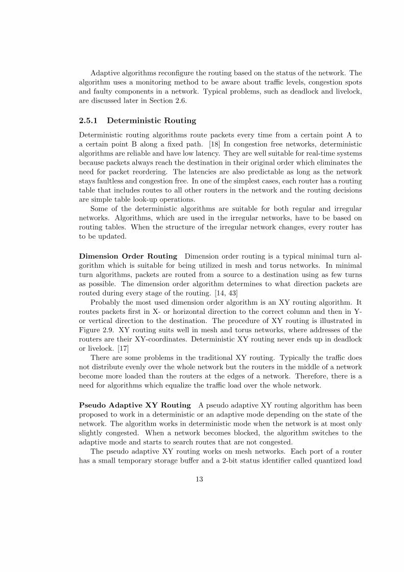
Dimension Order Routing Dimension order routing is a typical minimal turn al-gorithm which is suitable for being utilized in mesh and torus networks. In minimalturn algorithms, packets are routed from a source to a destination using as few turnsas possible. The dimension order algorithm determines to what direction packets arerouted during every stage of the routing. [14, 43]

Probably the most used dimension order algorithm is an XY routing algorithm. Itroutes packets first in X- or horizontal direction to the correct column and then in Y-or vertical direction to the destination. The procedure of XY routing is illustrated inFigure 2.9. XY routing suits well in mesh and torus networks, where addresses of therouters are their XY-coordinates. Deterministic XY routing never ends up in deadlockor livelock. [17]

There are some problems in the traditional XY routing. Typically the traffic doesnot distribute evenly over the whole network but the routers in the middle of a networkbecome more loaded than the routers at the edges of a network. Therefore, there is aneed for algorithms which equalize the traffic load over the whole network.

Pseudo Adaptive XY Routing A pseudo adaptive XY routing algorithm has beenproposed to work in a deterministic or an adaptive mode depending on the state of thenetwork. The algorithm works in deterministic mode when the network is at most onlyslightly congested. When a network becomes blocked, the algorithm switches to theadaptive mode and starts to search routes that are not congested.

The pseudo adaptive XY routing works on mesh networks. Each port of a routerhas a small temporary storage buffer and a 2-bit status identifier called quantized load

13

- -

6

6

A

B

Figure 2.9: XY routing from router A to router B.

value. The identifier tells the other routers if the router is congested and cannot acceptnew packets.

A router assigns priorities to incoming packets when there are more than one incom-ing packet arriving simultaneously. Packets from north have the highest priority, thensouth, east and finally packets incoming from west have the lowest priority. While thetraditional XY routing causes network loads more in the middle of the network than tothe lateral areas, the pseudo adaptive algorithm divides the traffic better over the wholenetwork. [17]

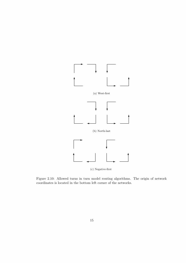
Turn Models Turn model algorithms determine turns which are and which are notallowed while routing packets through a network. Turn models are deadlock-free becausethe turn prevention eliminates the possibility to transmit packets in full circle. Threeexamples of turn model algorithms are presented below. [32]

1. West-first routing algorithm prevents all turns from any direction towards west.Therefore, the packets going west must be first transmitted as far towards west asnecessary. Routing packets towards west is not possible later on.

2. North-last routing algorithm disables turns away from north direction. Thus, thepackets which need to be routed towards north, must be first moved in east-west-dimension and finally towards north to the destination.

3. Negative-first routing algorithm allows all other turns except turns from a positivedirection to a negative direction. The network is considered as a coordinate systemwhere the origin is in the bottom left corner and the positive directions are frombottom to top and from left to right. Packet routings in negative directions mustbe done before anything else.

Allowed turns in these three turn model algorithms are illustrated in Figure 2.5.1.

14

-

?

6

-

6

?

(a) West-first

?

6

-

6

?

�

(b) North-last

6

-

6

?

�

-

(c) Negative-first

Figure 2.10: Allowed turns in turn model routing algorithms. The origin of networkcoordinates is located in the bottom left corner of the networks.

15

Shortest Path Routing Shortest path routing algorithms transfer packets alwaysalong the shortest path from a sender to a receiver. A distance vector routing algorithmis the most basic shortest path routing algorithm. Each router has a routing tablethat contains information about neighbor routers and all possible packet destinations.Routers exchange routing table information with each other and this way keep theirown tables up to date. Routers route packets by calculating the shortest path based ontheir routing tables and then send packets forward. Distance vector routing is a simplemethod because each router does not have to know the structure of the whole network.[5]

Link state routing is somewhat more complex than the distance vector routing. Thebasic idea is the same as in the distance vector routing, but in the link state routingalgorithm each router shares its routing table with every other router in the network. Thelink state routing presented for Network-on-Chip systems is a little bit customized versionof the traditional distance vector routing. The routing tables covering the whole networkare stored in memories of routers already during the manufacturing phase. Routers usetheir routing table updating mechanisms only if there are remarkable changes in thestructure of the network or if some new faults emerge. [5]

Source Routing In source routing a sender makes all routing decisions concerning thecomplete routing path of a packet. The whole route is stored in the header of a packetbefore sending, and routers along the path do the routing following the predefined routingpath.

Arbitration look ahead scheme (ALOAS ) is a faster version of source routing. Infor-mation of a routing path has been supplied to routers along the path before the packetsare even sent. Route information moves along a special channel that is reserved only forthis purpose. [16, 35, 71]

Contention-free routing is an algorithm based on routing tables and time divisionmultiplexing (TDM). Each router has a routing table that includes corresponding outputports and time slots to every potential sender–receiver pairs. Contention-free routingalgorithm is used in Philips Æthereal NoC system and it is also called as a clockworkrouting. [24, 39, 48, 50]

Destination-tag Routing A destination-tag routing algorithm is a kind of an in-verted version of the source routing algorithm. The sender stores the address of the des-tination, also known as a destination-tag, to the header of a packet. Every router makesrouting decisions independently based on the address of the receiver. The destination-tag routing is also known as floating vector routing. [14, 71] The routing decisions arebased on routing tables which are stored in every router.

Topology Adaptive Routing Deterministic routing algorithms can be improved byadding some adaptive features to them. The algorithm works like a basic deterministicalgorithm but it has one feature which makes it suitable for dynamic networks. A central

16

controller can update the routing tables of the routers if necessary. A correspondingalgorithm is also known as an online oblivious routing. [8] The cost and latency ofthe topology adaptive routing algorithm are near to the costs and latencies of basicdeterministic algorithms. An advantage of topology adaptiveness is its suitability toirregular and dynamic networks.

2.5.2 Stochastic Routing Algorithms

Stochastic routing algorithms are based on coincidence and an assumption that everypacket sooner or later reaches its destination. Stochastic algorithms are typically simpleand fault-tolerant. Throughput of data is especially good but as a drawback, stochasticalgorithms use plenty of network resources.

Stochastic routing algorithms determine time to live (TTL) of packets. It is a timehow long a packet is allowed to move around in the network. After the predefined timehas been reached, the packet will be dropped from the network. When a packet isdropped, the sender of the packet has to be notified so that it could resend the data. Afew stochastic routing algorithms are presented below.

Probabilistic Flood The simplest stochastic routing algorithm is the probabilisticflooding algorithm. [19, 52] Routers send a copy of an incoming packet in all possibledirections without any information about the location of the destination of a packet.The copies of a packet diffuse over the whole network similarly as a flood. Finally, mostprobably at least one of the copies will arrive at its destination and the redundant copieswill be removed.

Directed Flood A directed flood routing algorithm is an improved version of proba-bilistic flood. It directs packets approximately in the direction where their destination islocated. The main advantage of a directed flood is its lower network resource consump-tion compared with a probabilistic flood. [20, 53]

Random Walk A random walk algorithm sends a predetermined amount of copiesof a packet to a network. Every router along the routing path sends incoming packetsforward through some of its output ports. The packets are directed in the same way asin the directed flood algorithm. The network resource load, caused by a random walkrouting algorithm, is lower than the load of the two stochastic algorithms presentedabove. [53]

Valiant’s Random Algorithm Valiant’s random algorithm is a partly stochasticrouting algorithm. One main problem in deterministic routing algorithms is that theycause irregular load in a network. The load is typically especially high in the middleareas of the network. Valiant’s random algorithm equalizes traffic load on networksthat have a good path diversity. First the algorithm randomly picks one intermediatenode and routes packets to it. Then the packets are simply routed to their destination.

17

Routing from beginning to the intermediate node and then to the destination are doneusing a deterministic routing algorithm. [68]

IVAL (Improved VALiant’s randomized routing) is an improved version of the Valiant’srandom algorithm. It is similar to turn around routing. At the first stage of the algo-rithm packets are routed to a randomly chosen point between the sender and the receiverby using oblivious dimension order routing. The second stage of the algorithm worksalmost equally, but this time the dimensions of the network are handled in reverse order.Deadlocks are avoided in IVAL routing by assigning virtual channels to the physicalchannels of a router. [67]

2.5.3 Adaptive Routing

Adaptive routing algorithms are able to reconfigure the routing during run-time basedon the status of the network. Several adaptive routing algorithms for Network-on-Chipare presented below.

Minimal Adaptive Routing A minimal adaptive routing algorithm routes packetsalways along the shortest network path. The algorithm is effective when more thanone minimal, or as short as possible, paths between a sender and a receiver exist. Thealgorithm uses the route which is least congested. [14]

Fully Adaptive Routing A fully adaptive routing algorithm always uses a routewhich is least congested regardless of the length of the route. Typically, an adaptiverouting algorithm ranks alternative congestion free routes to order of superiority. Thenthe shortest route used. [14]

Congestion Look Ahead A congestion look ahead algorithm gets information ofcongestion from other routers. Based on this information the routing algorithm candirect packets to bypass the congestion spots. [35]

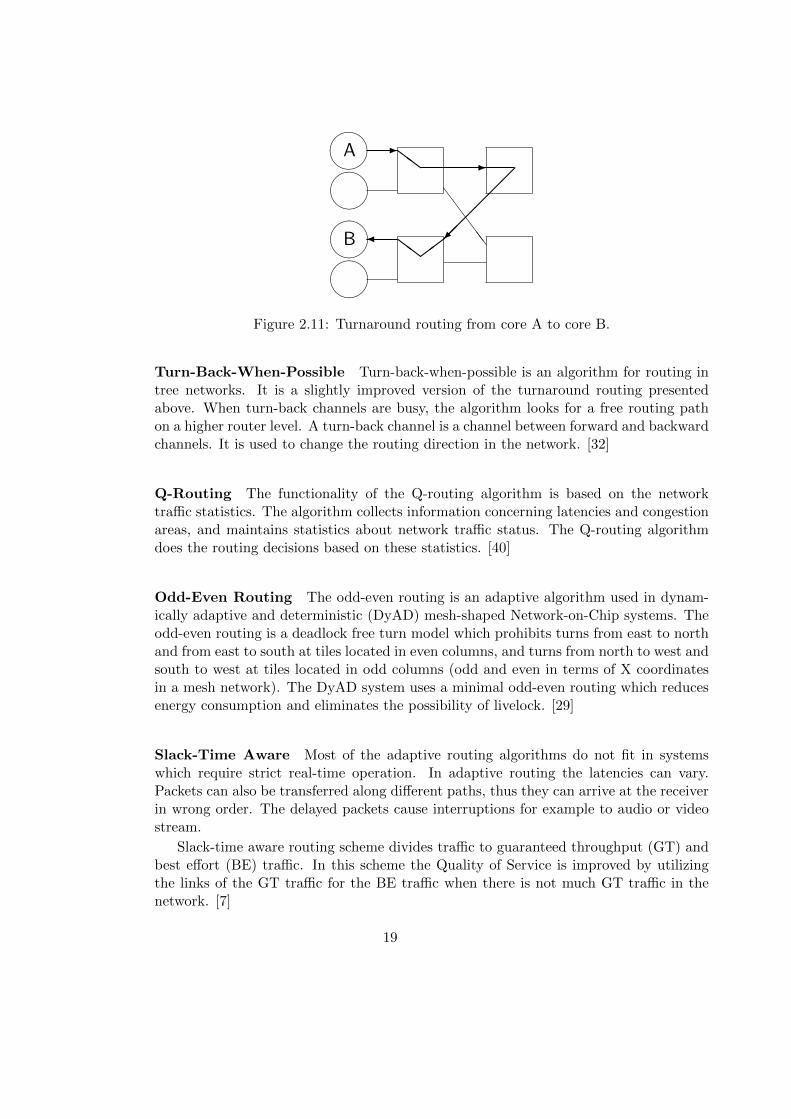
Turnaround Routing Turnaround routing is a routing algorithm for butterfly andfat-tree networks. The senders and receivers are all on the same side of the network,as illustrated in Figure 2.11. Packets are at first routed from the sender to some of theintermediate nodes located on the other side of the network. In this node, the packets areturned around and then routed to the destination. The routing from the intermediatenode to the receiver is done with the destination-tag routing algorithm.

Routers in turnaround routing are bidirectional which means that packets can flowthrough a router in both forward and backward directions. The algorithm is deadlock-free because packets only turn around once from a forward channel to a backward chan-nel.

18

����

����

��������-ZZ -

���

���

��Z

Z�

SSSSS

A

B

Figure 2.11: Turnaround routing from core A to core B.

Turn-Back-When-Possible Turn-back-when-possible is an algorithm for routing intree networks. It is a slightly improved version of the turnaround routing presentedabove. When turn-back channels are busy, the algorithm looks for a free routing pathon a higher router level. A turn-back channel is a channel between forward and backwardchannels. It is used to change the routing direction in the network. [32]

Q-Routing The functionality of the Q-routing algorithm is based on the networktraffic statistics. The algorithm collects information concerning latencies and congestionareas, and maintains statistics about network traffic status. The Q-routing algorithmdoes the routing decisions based on these statistics. [40]

Odd-Even Routing The odd-even routing is an adaptive algorithm used in dynam-ically adaptive and deterministic (DyAD) mesh-shaped Network-on-Chip systems. Theodd-even routing is a deadlock free turn model which prohibits turns from east to northand from east to south at tiles located in even columns, and turns from north to west andsouth to west at tiles located in odd columns (odd and even in terms of X coordinatesin a mesh network). The DyAD system uses a minimal odd-even routing which reducesenergy consumption and eliminates the possibility of livelock. [29]

Slack-Time Aware Most of the adaptive routing algorithms do not fit in systemswhich require strict real-time operation. In adaptive routing the latencies can vary.Packets can also be transferred along different paths, thus they can arrive at the receiverin wrong order. The delayed packets cause interruptions for example to audio or videostream.

Slack-time aware routing scheme divides traffic to guaranteed throughput (GT) andbest effort (BE) traffic. In this scheme the Quality of Service is improved by utilizingthe links of the GT traffic for the BE traffic when there is not much GT traffic in thenetwork. [7]

19

Hot-Potato Routing The hot-potato routing algorithm routes packets without tem-porarily storing them in a buffer memory of a router. Packets are moving all the timewithout stopping until they reach their destination. When one packet arrives at a router,the router forwards it immediately towards its destination. However, if there are twopackets going in the same direction simultaneously, the router directs one of the packetsin some other direction. This other packet can possibly flow away from its destination.This occasion is called as misrouting. In the worst case, packets can be misrouted faraway from their destination and misrouted packets can interfere with other packets. Therisk of misrouting can be decreased by waiting short random time before sending eachpacket. Cost of the hot-potato routing is quite low because the routers do not need anybuffer memory to store packets during routing. [21]

2.6 Network Problems

The two main categories of routing algorithms are deterministic and adaptive algorithms.Problems on deterministic routing, or routing without the information of the state of thenetwork, typically arise when a network starts to block traffic. The only solution to theseproblems is to wait for the reduction of traffic, and try again. Deadlock and starvationare potential problems in deterministic algorithms as well as in adaptive algorithmswhich adapt the routing based on the state of the network. Additionally, livelock canoccur in systems utilizing adaptive routing algorithms.

Deadlock Deadlock is a situation where two or more packets are waiting each otherto be routed forward. All the packets reserve some resources and both are waiting eachother to release the resources. Routers do not release the resources before they get thenew resources and so the routing is locked. [65]

Deadlock situation can be solved by removing one of the packets temporary or per-manently. However, better solution would be to design the routing algorithm in a waythat it avoids the deadlocks.

Livelock Livelock occurs when a packet keeps spinning around its destination withoutever reaching it. This problem exists in routing algorithms which do not route the packetsalways along the shortest path between the sender and the destination. Livelock shouldbe cut out to guarantee throughput of packets. [65]

There are a couple of solutions to avoid the livelock. Time to live (TTL) countercounts how long a packet has travelled in the network. When the counter reaches somepredetermined value, the packet will be removed from the network. However, packetdropping is rarely an absolutely good solution because the data payload is lost at leastuntil a retransmit. Another solution is to give packets a priority which is based on theage of a packet. The oldest packet always finally gets the highest priority and will berouted forward.

20

Starvation Using different priorities can cause a situation where some packets withlower priorities never reach their destinations. This applies to prioritization which is notbased on the age of a packet. The starvation occurs when packets with higher prioritiesreserve resources all the time and the lower priority packets do not get any resources tobe transmitted. Starvation can be avoided by using a fair routing algorithm, which isan algorithm without fixed priorities, or reserving some bandwidth only for low-prioritypackets. [42]

2.7 Summary

This chapter presented essential principles and basics of Network-on-Chip paradigm.Basic components of NoC were presented and different network topologies were studied.Vital details, including network traffic classification, network flow control as well asrouting algorithms were presented. Finally, typical problems arising in Networks-on-Chip were studied.

21

22

Chapter 3

Monitoring on Network-on-Chip

Network-on-Chip (NoC) is a promising interconnection paradigm for future high-performanceintegrated circuits [9, 16, 49] and its features and potentiality have been discussed inChapter 2. To enable the full potential of the NoC there is a need for monitoring servicesto diagnose the system functionality, to optimize the performance and to do run-timesystem reconfiguration. The reconfiguration is required to keep the system working withreasonable performance regardless of faults and unbalanced load in the system [64].

Monitoring services can be roughly divided into two categories based on their mainpurpose: system diagnostics and traffic management. The former aims to improve thereliability and performance of the computational parts while the latter concentrates tothe same issues in the communication resources. It includes fault detection, performancemonitoring as well as computation load management. The other part of the monitoringservices, the traffic management, focuses on the communication infrastructure which en-ables the interaction between computational components. Traffic management containsfeatures to maximize communication infrastructure performance and reliability while op-timizing its power consumption. It is used to balance the utilization of communicationresources and to avoid congestion in the network as well as to reconfigure the routingin the network in case of faults or congestion related problems. The goal is to main-tain the network functionality regardless of above-mentioned issues. The core of trafficmanagement is network monitoring which observes network components and delivers theobserved information so that it can be used to reconfigure the network. Typically thereis a monitoring system to collect traffic information from the network and an adaptiverouting algorithm which adapts its operation when the conditions in the network change(see Section 2.5).

Two types of information are collected in network monitoring: traffic status in thenetwork and locations of faults in the network. Traffic statuses can be observed fromdifferent parts of a network: router activity, router FIFO occupancy, or link utilization,for instance. Fault information can cover the faultiness of different network components:routers or links, for instance. A network component is considered as faulty when itdoes not work as it should by its specification. The network components have to have

23

mechanisms to detect these faults [26]. There are several methods to do the detection.For instance, faulty links can be detected using methods which are based on the usageof spare resources or error control coding [37, 10]. Traffic management is discussed andanalyzed in Chapter 6 while a significant part of a system management is studied inChapter 7.

In a Network-on-Chip data are typically transferred as packets which have a desti-nation address and an identifier which shows the type and purpose of the packet. Thesepacket types can include for instance data packets, monitoring packets or mapping pack-ets. All these packets are identical in terms of data transfer in the network. They aretransferred in a network from a sender to a destination based on a routing algorithm.Identifiers are used to recognize packets so that every packet is forwarded to right com-ponent or handled in correct process. The majority of packets are data packets whichare used to transfer payload data from a core to another. The control packets, whichinclude for instance monitoring and mapping packets, transfer some information whichis used for system management purposes. Mapping packets are discussed in Chapter7. Network monitoring related data are transferred in monitoring packets. When amonitoring packet is received in the destination indicated by its destination address, thepacket is forwarded to the monitor component for further processing.

The NoC monitoring systems which use shared communication resources transfer thenetwork status data using monitoring packets. When centralized or clustered monitoringstructures are used, these packets have to be initialized in probes, routed from probesto a monitor and from the monitor to the routers. Centralized control has its strengthsand it is essential for several tasks. However, to optimize performance some of thetraffic management tasks could be carried out with simpler distributed, or dynamicallyclustered, monitoring structures to decrease the load of the centralized control system.[55]

3.1 Purpose of Monitoring

The main purposes of monitoring in Network-on-Chip include traffic management andsystem diagnostics. Traffic management related monitoring is mainly based on the ob-servation of communication resource usage. System diagnostics can be also applied fortraffic management purposes for instance by using fault data for router reconfiguration.

System diagnostics can include various information which is collected for statisticalor system control purposes. One application of system diagnostics is task mapping whichis studied in more detail later on.

3.1.1 Traffic Management

To enable the maximum throughput, the communication resource utilization has to bebalanced so that all the resources are utilized and the congestion is avoided. Adaptiverouting and route reconfiguration are keys to balance traffic and to avoid congestion[14, 18, 57]. Traffic management should distribute traffic evenly over the whole network

24

and all the usable resources so that all the resources are used on their optimal load andhighly loaded traffic hot spots are not formed.

Implementation of traffic management requires network monitoring; there should bea monitoring system which collects the information needed to optimize the routing. Thisinformation includes knowledge of current traffic conditions as well as knowledge con-cerning network functionality and faults. Basically, it is not necessary to have completeknowledge of the network status in each router; a router should have information onthe network state at the region around it so that it can direct the traffic in the leastcongested directions.

3.1.2 Fault Detection

Modern integrated circuits are sensitive to transient faults. Because of a complex manu-facturing process it is also possible that the circuits can contain permanent manufactur-ing faults which can occur as run-time errors e.g. due to electromigration. [54, 66, 70]The objective is to design a system that tolerates faults or recovers from errors causedby faults. The circuits should also be capable to reliable operation even though thereare a few permanent faults.

The detection of faults requires a monitoring system to locate them and to providethe information for other components. For instance in the case of a manufacturingfault, the system could disable the faulty component and migrate its tasks to some othercomponent. This kind of operation requires redundancy in the system to enable taskmigration.

The fault detection is also a part of the traffic management. When there are faultsin the communication infrastructure, the monitoring system can detect them and informthe system to reconfigure the routing through faultless communication resources.

3.1.3 Task Management

A monitoring structure can be applied for different management and reconfigurationtasks in a Network-on-Chip. An essential task, included in the system management, istask mapping.

Typically tasks are mapped to cores at the initialization phase of system operation.The system diagnostic features of a NoC monitoring system make it possible to collecttask mapping related statistics and use this data to map new tasks run-time. The goal isto find a suitable core which is able to execute the new task and at the same time to keepthe computational load evenly distributed over the system. Balanced load distribution,both computational and communication load, is essential because that way the maximumperformance can be achieved without formation of highly loaded hot spots. These hotspots are unfavorable in terms of performance as well as unbalanced power consumptionand heat dissipation. Task mapping on NoC is studied in Chapter 7.

25

3.2 Monitoring Structures

An NoC monitoring system has the same main requirements as the NoC itself; it shouldbe flexible, scalable and it should also be capable of real-time operation [12]. Scalabilityand flexibility ensure that a monitoring system can be used in different sized Networks-on-Chip without a time consuming redesigning process. A monitoring system itselfshould also be fault tolerant. A network monitoring structure consists of monitoringunits (monitors) and probes as well as communication resources (e.g. routers), or wires,to connect these components to each other and to the NoC, as illustrated in Figure 3.1.The monitors are computational components which control the monitoring process anddeliver observed data to its clients. The probes are connected to network components,e.g. routers, network interfaces or links, whose functionality they observe and deliverthe observed data to the monitoring units.

A monitoring structure can have dedicated resources for communication betweenprobes and monitors, or it can share the resources of the data network. In our research,we focus on shared-resource structures which require less additional resources than dedi-cated structures. We have also paid attention to dedicated resources for serial monitoringcommunication between monitors. In shared-resource structures non-intrusive operationof the monitoring system is a significant issue while in the serial monitoring communi-cation the delays are crucial in terms of usefulness of the monitoring data.

If the network resources are dedicated for communication between the probes and themonitors, the probes can be controlled from the monitors. Otherwise the probes have tobe more autonomous to be able to communicate over the shared packet switched network.Monitors are computational components which control the monitoring. Monitors collectthe monitoring data, exchange the data with other monitors and provide informationfor network components which can use it to reconfigure their operation. The systemdiagnostics can share the resources of the traffic management but may also require

6

?

6

?

-�

?6

-�

?6

� -

?

6

?

6

Router

Probe

Monitor

Router

Probe

Monitor

Figure 3.1: Network components and their connections.

26

dedicated components e.g. probes which are attached to the computational resources andcentralized control devices which are not necessarily required in the traffic management.

Depending on the purpose, requirements and operational principles the monitoringsystem can have centralized, clustered, distributed or localized structure. The structureof the monitoring system defines how the monitoring data are delivered to the othercomponents in the system and which of the components are able to access this informa-tion. Monitoring structure defines the number and type of monitors and probes, theirplacement, connections and tasks. A centralized monitoring structure has one centralmonitor and several probes that observe the data and deliver it to the monitor. In cen-tralized structure, the central monitor has complete overall knowledge of the networkbut it causes significant amount of monitoring related traffic in the network. A clusteredmonitoring structure has a few cluster monitors and several probes. The network isdivided into subnetworks, clusters, each of them having a cluster monitor and severalprobes. The complete network knowledge can be reached using inter-cluster commu-nication but most of the tasks can be executed inside a cluster. However, a clusteredstructure still causes a considerable amount of monitoring traffic. [55]

Our research focuses on a scalable NoC monitoring structures where the knowledgeof network status is spread widely enough over the network. There are two main factorstaken into account while designing our NoC architecture. First, the structure shouldbe not only aware of traffic but also aware of network faults so that network-level faulttolerance can be actively maintained during routing. Second, the structure should alsobe fully scalable to any mesh size. All the probes and monitors are identical and theywork autonomously without any centralized control. The structure should also be easilyreconfigurable for new applications which could turn up later on. The presented ideascan be adapted to NoC topologies of a different kind but due to its popularity, we havedecided to concentrate on the mesh topology.

3.2.1 Centralized Monitoring

In a system with centralized monitoring there is a central monitoring unit and a numberof probes which are attached to the network components. Probes deliver the data to thecentral monitor which collects the monitoring data and delivers information all aroundthe system. Centralized monitoring has advantages on performance monitoring and oncollecting statistical information from the system. Resource allocation for computationaltasks may also require centralized control. However, a centralized monitoring system isinflexible and scales poorly. When the size of a system increases the average distancebetween the probes and the central monitoring component increases as well. Long dis-tances between the probes and monitors increase the probability of network faults andcause more traffic to the network especially if the monitoring system uses shared com-munication resources. In a highly loaded network, this additional traffic can increase theprobability of congestion. In centrally monitored systems, all the monitoring is carriedout in a single component which makes it very susceptible to faults.

NoC monitoring systems have been presented in several papers. A dedicated control

27

network is used in a centralized operating system controlled NoC [47]. It has separatedata NoC and control NoC from which the latter is used for centralized monitoring andcontrol. An operating system controls the network management through the dedicatedcontrol NoC by collecting data from the processing elements (PE).

Another centralized NoC monitoring implementation is presented in [44] where adedicated embedded processor is used to observe FIFO occupancies and packet transferlatencies. The monitoring processor is connected to routers with dedicated links. Thecollected data are used for partial dynamic reconfiguration purposes.

In [13] a transaction monitoring system for Æthereal NoC [24] has been presented.This system, which monitors transactions in NoC components, can be configured toshared or dedicated communication resources. The probes monitor bit-level data whichhave been interpreted as transactions and forwarded to a centralized monitor (MonitoringService Access point).

A congestion control system which monitors links and uses shared communicationresources is presented in [69]. It measures the amount of congestion by monitoring linkutilization and adjusts data sources to control congestion. All these systems include acentralized monitoring unit which collects the observed data and controls the systemoperation.

All the above implementations are meant for traffic management while a monitoringsystem for run-time optimization and resource allocation was presented in [23]. Theprobes are implemented within NIs and they observe throughput, latency and eventoccurrences in PEs.

3.2.2 Clustered Monitoring

In clustered and distributed NoC monitoring there is no centralized monitoring unitwhere the global monitoring data are collected. In the clustered approach the systemis divided into subsystems, clusters, each of which has a cluster monitoring unit wherethe monitoring data from the probes in the cluster is collected. The cluster monitorscan exchange information with each other. A clustered monitoring structure with thecluster size of four is presented in Figure 3.2. If the cluster size is relatively large thenumber of monitors can be kept low. However, the smaller the cluster is, the less effecta faulty monitor has on the system operation. Communication distances are naturallyalso shorter when cluster size is small.

ROAdNoC is a runtime observability infrastructure which uses shared communica-tion resources and basically has a clustered structure but can also utilize centralizedcontrol if necessary. It observes routers and NIs and collects error, run-time and func-tional information. [2] A notably similar structure is presented in [12]. Both of thesestructures utilize event-based communication and the latter can be used to monitor allthe NoC components. On event-based communication, the probes generate events fromthe monitoring data which allows the monitoring data abstraction and leads to com-munication overhead reduction. A clustered monitoring structure is presented also in[41]. It collects information from the routers, identifies which senders cause the conges-

28

tion, and does traffic shaping by restraining these sender cores. The control data havededicated communication resources.

3.2.3 Localized Monitoring

Localized monitoring is the simplest monitoring scheme to be implemented in an NoC.Typically there are no actual monitor components but the probed values are used locallywithout further processing or they are delivered to the neighboring routers. The localizedmonitoring is typically used in adaptive routing where the probes observe output channelreservation or the router utilization levels.

Localized monitoring systems have been presented in several papers as a part ofadaptive routing mechanism; for example for Nostrum NoC [46]. In the basic version ofthe Nostrum NoC there is a probe on each router. Those provide traffic level informationfor the neighboring routers. The difference from distributed structures is that there areno separate monitors which collect the information and exchange it with each other.

RM

P

RM

P

RM

P

RM

P

R

P

R

P

R

P

R

P

R

P

R

P

R

P

R

P

R

P

R

P

R

P

R

P

Cluster2

Cluster4Cluster3

Cluster1

@@@@

@@ @@

@@@@

@@ @@

@@@@

@@ @@

@@@@

@@ @@

Figure 3.2: Clustered monitoring (cluster size: 4). Probes (P) and monitors (M) areintegrated into the routers (R).

29

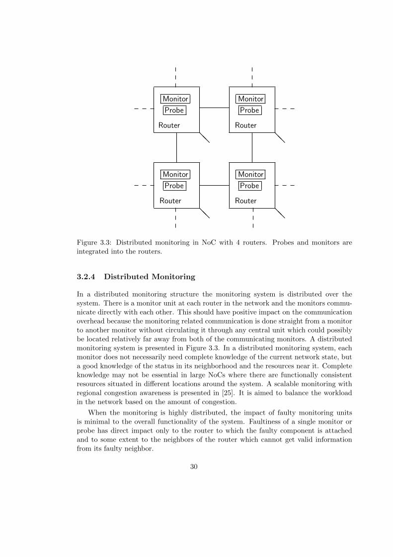
Probe

Router

Monitor

Probe

Router

Monitor

Probe

Router

Monitor

Probe

Router

Monitor

@@

@@

@@

@@

Figure 3.3: Distributed monitoring in NoC with 4 routers. Probes and monitors areintegrated into the routers.

3.2.4 Distributed Monitoring

In a distributed monitoring structure the monitoring system is distributed over thesystem. There is a monitor unit at each router in the network and the monitors commu-nicate directly with each other. This should have positive impact on the communicationoverhead because the monitoring related communication is done straight from a monitorto another monitor without circulating it through any central unit which could possiblybe located relatively far away from both of the communicating monitors. A distributedmonitoring system is presented in Figure 3.3. In a distributed monitoring system, eachmonitor does not necessarily need complete knowledge of the current network state, buta good knowledge of the status in its neighborhood and the resources near it. Completeknowledge may not be essential in large NoCs where there are functionally consistentresources situated in different locations around the system. A scalable monitoring withregional congestion awareness is presented in [25]. It is aimed to balance the workloadin the network based on the amount of congestion.

When the monitoring is highly distributed, the impact of faulty monitoring unitsis minimal to the overall functionality of the system. Faultiness of a single monitor orprobe has direct impact only to the router to which the faulty component is attachedand to some extent to the neighbors of the router which cannot get valid informationfrom its faulty neighbor.

30

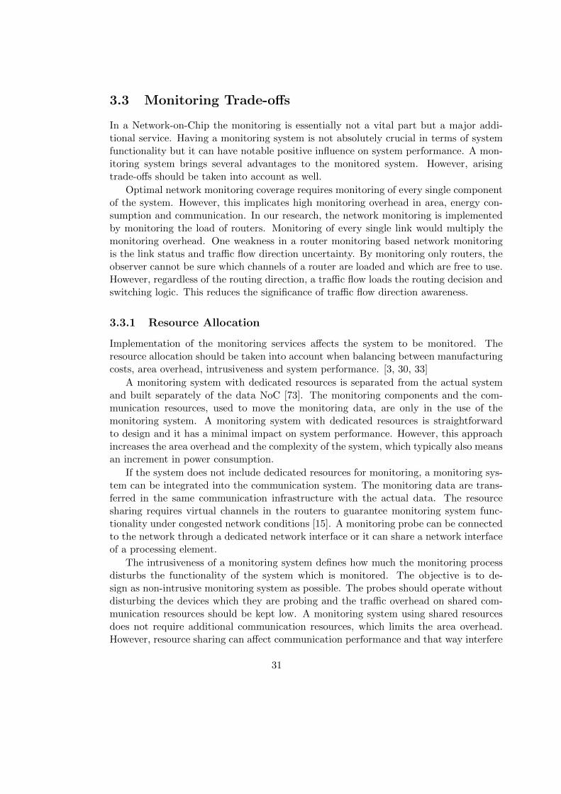
3.3 Monitoring Trade-offs

In a Network-on-Chip the monitoring is essentially not a vital part but a major addi-tional service. Having a monitoring system is not absolutely crucial in terms of systemfunctionality but it can have notable positive influence on system performance. A mon-itoring system brings several advantages to the monitored system. However, arisingtrade-offs should be taken into account as well.

Optimal network monitoring coverage requires monitoring of every single componentof the system. However, this implicates high monitoring overhead in area, energy con-sumption and communication. In our research, the network monitoring is implementedby monitoring the load of routers. Monitoring of every single link would multiply themonitoring overhead. One weakness in a router monitoring based network monitoringis the link status and traffic flow direction uncertainty. By monitoring only routers, theobserver cannot be sure which channels of a router are loaded and which are free to use.However, regardless of the routing direction, a traffic flow loads the routing decision andswitching logic. This reduces the significance of traffic flow direction awareness.

3.3.1 Resource Allocation

Implementation of the monitoring services affects the system to be monitored. Theresource allocation should be taken into account when balancing between manufacturingcosts, area overhead, intrusiveness and system performance. [3, 30, 33]

A monitoring system with dedicated resources is separated from the actual systemand built separately of the data NoC [73]. The monitoring components and the com-munication resources, used to move the monitoring data, are only in the use of themonitoring system. A monitoring system with dedicated resources is straightforwardto design and it has a minimal impact on system performance. However, this approachincreases the area overhead and the complexity of the system, which typically also meansan increment in power consumption.

If the system does not include dedicated resources for monitoring, a monitoring sys-tem can be integrated into the communication system. The monitoring data are trans-ferred in the same communication infrastructure with the actual data. The resourcesharing requires virtual channels in the routers to guarantee monitoring system func-tionality under congested network conditions [15]. A monitoring probe can be connectedto the network through a dedicated network interface or it can share a network interfaceof a processing element.

The intrusiveness of a monitoring system defines how much the monitoring processdisturbs the functionality of the system which is monitored. The objective is to de-sign as non-intrusive monitoring system as possible. The probes should operate withoutdisturbing the devices which they are probing and the traffic overhead on shared com-munication resources should be kept low. A monitoring system using shared resourcesdoes not require additional communication resources, which limits the area overhead.However, resource sharing can affect communication performance and that way interfere

31

with the actual operation of the system. Shared-resource monitoring systems are fas-cinating because of their minimal added complexity. Nevertheless, due to intrusivenessaspects, shared-resource monitoring systems have to be designed carefully. [13]

3.4 Fault Tolerance of Monitoring Systems

The monitoring systems can be used to improve the fault tolerance of NoCs as was de-scribed in Section 3.1.2. However, the monitoring systems themselves are also vulnerableto faults which has to be taken into account in the design process.

The faults can occur in the data moved between monitors or they can affect tothe functionality of the actual monitor components. If a monitoring system shares theresources with an NoC, the fault tolerance methods utilized to the actual data can beapplied also to the monitoring data. Otherwise, if a monitoring system has dedicatedcommunication resources there should be separate fault tolerance mechanisms for these.The fault tolerance mechanisms for data could be e.g. triple modular redundancy, orerror control codes [10, 31, 36, 45].

To ensure the intended functionality of the actual monitor components a built-inself-test mechanism could be implemented [72]. Self-test mechanism regularly checksthe functionality of a component so that faulty components can be recognized, disabledand possibly replaced with spare resources. Similar mechanisms for NoC routers andlinks have been implemented previously in [22] and [27] correspondingly.

3.5 Summary

Introduction to monitoring in Networks-on-Chip were given in this chapter. At first,the purposes of network monitoring were studied. Different monitoring structures werepresented. Finally, trade-offs of monitoring and fault tolerance of monitoring systemswere discussed.

32

Chapter 4

Dynamically ClusteredDistributed Monitoring

Scalability is an essential feature of Networks-on-Chip [9]. The distributed approachmakes it possible to scale the monitoring system similarly as the actual NoC can bescaled. Centralized monitoring solutions scale poorly and are built separately with theNoC. While a centralized structure can be feasible on a small system the limited scal-ability is against the main principles of the NoC paradigm: an NoC should be fullyscalable in any size and its performance should not be weakened when the size of thesystem is increased. Our hypothesis is that the use of distributed monitoring systemshas a positive impact on traffic overhead caused by network monitoring, which decreasesthe demand for dedicated resources. The distributed monitoring structure has poten-tial to be more fault tolerant than the centralized and clustered systems because thefaultiness of a single component has an immediate influence only to just a few othercomponents. Faultiness of a centralized component may endanger the functionality ofthe whole system.

The distributed monitoring system has several potential advantages when comparedwith the centralized and clustered monitoring. In centralized and clustered monitoringthe monitoring data have to be moved to the monitoring unit for processing and thenback to the routers before the information can be exploited. In a distributed system,the monitor receives information from its local probe and its neighbors and performs therequired processing. It is also possible to implement centralized control at the operatingsystem level while the traffic management, for instance, uses distributed monitoring.

4.1 Dynamically Clustered Monitoring Structure

We propose an NoC monitoring structure which is originally focused on traffic man-agement, including routing reconfiguration and traffic load balancing, but can also beutilized for system reconfiguration and problem recovery for instance in the case offaults or congestion. Fortunately, the origin of a problem is not relevant from the traffic

33

management point of view.

Scalable NoC monitoring is based on an idea that there is no need for comprehen-sive status information of the whole network in a single centralized monitoring unit. Toguarantee high and predictable performance the congestion should be avoided before-hand. We propose that efficient traffic management can be achieved without centralizednetwork monitoring. When the traffic overhead of the traffic management is minimized,the remaining bandwidth can be used for normal data traffic as well as essential centrallycontrolled features which cannot be realized with a distributed structure. Most of thetraffic management tasks can be executed without centralized control, thus, there is noreason to waste resources on these purposes.

In our monitoring approach every router has its own status which is based on theutilization level of the router and its neighbors. Every router has up-to-date informa-tion about the statuses of five or the twelve closest neighbor routers around it. Thismonitoring protocol can be implemented in centralized, clustered or distributed moni-toring systems. The distributed version of this monitoring structure is also called thedynamically clustered structure.

A dynamic cluster is the area around a router from where the router status have beencollected and to where the status of the router has been delivered. In statically clusteredsystems (see Section 3.2.2) the cluster borders are fixed and that way the routers nearthe cluster borders have unequal amount of status information from neighbor routersbecause some neighbors are in the same cluster and others in a different cluster as therouter itself. In dynamically clustered structure the router is always placed in the middleof its own dynamic cluster which balances the amount of neighbor status data.

Figure 4.1 illustrates an NoC with 100 routers. Every router has a dynamic clusterbut only three of them are illustrated to keep the presentation readable. A router hasthe status information of the components in its own dynamic cluster. This informationdrifts from the network components to a monitor along simple neighbor to neighborinformation exchange. The clustered structures, presented earlier in the Section 3.2.2are statically clustered, which means that the borders of the clusters are fixed.

In statically clustered systems, the cluster monitor defines an overall status of its localcluster. This overall status is delivered to the neighboring clusters where it is forwardedto the routers. In a dynamically clustered structure, every router has an equal amountof neighbor status information. This differs from statically clustered structures wherethe amount of neighbor data depends on the location of a router in a cluster. Therouters which are situated near the edges and corners of static clusters have inaccurateneighbor status knowledge compared to the routers situated in the middle of a cluster.In a centralized implementation, the accuracy of monitoring statuses is on the same levelwith the distributed implementations. The difference is that in the centralized systemsthe status update requires a large amount of data to be transferred between routers andthe central monitoring unit (see Section 3.2.1).

The presented monitoring systems can be also used on small system reconfigurationtasks which do not require centralized control. Reconfiguration messages can be broad-casted over the monitoring system all around the network. The traffic diffusion analysis,

34

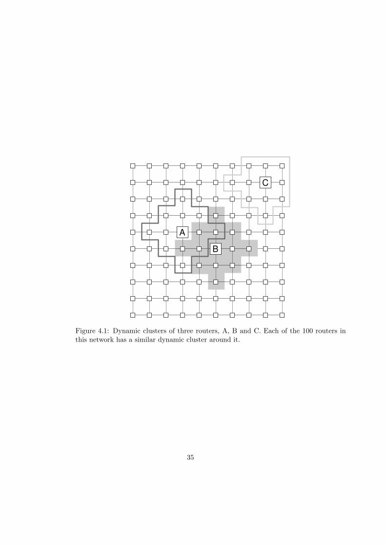
A

B

C

Figure 4.1: Dynamic clusters of three routers, A, B and C. Each of the 100 routers inthis network has a similar dynamic cluster around it.

35

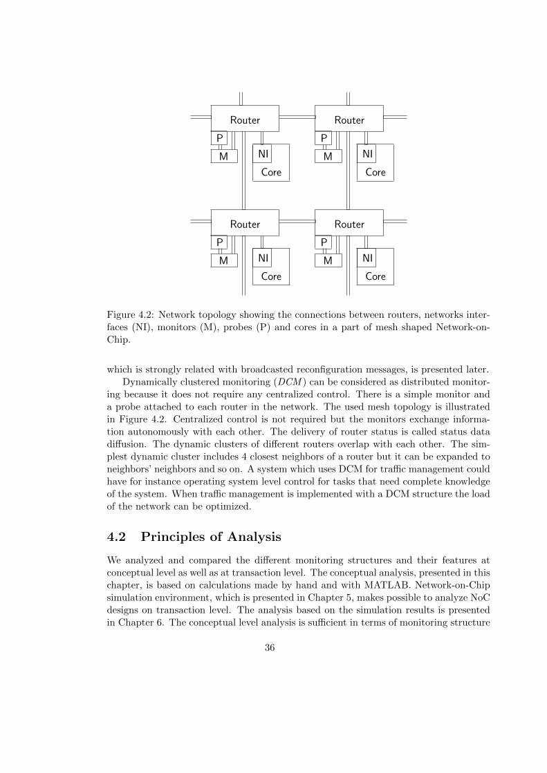
Core

NI

Core

NI

Core

NI

Core

NI

P

M

P

M

P

M

P

M

Router Router

RouterRouter

Figure 4.2: Network topology showing the connections between routers, networks inter-faces (NI), monitors (M), probes (P) and cores in a part of mesh shaped Network-on-Chip.

which is strongly related with broadcasted reconfiguration messages, is presented later.Dynamically clustered monitoring (DCM ) can be considered as distributed monitor-

ing because it does not require any centralized control. There is a simple monitor anda probe attached to each router in the network. The used mesh topology is illustratedin Figure 4.2. Centralized control is not required but the monitors exchange informa-tion autonomously with each other. The delivery of router status is called status datadiffusion. The dynamic clusters of different routers overlap with each other. The sim-plest dynamic cluster includes 4 closest neighbors of a router but it can be expanded toneighbors’ neighbors and so on. A system which uses DCM for traffic management couldhave for instance operating system level control for tasks that need complete knowledgeof the system. When traffic management is implemented with a DCM structure the loadof the network can be optimized.

4.2 Principles of Analysis

We analyzed and compared the different monitoring structures and their features atconceptual level as well as at transaction level. The conceptual analysis, presented in thischapter, is based on calculations made by hand and with MATLAB. Network-on-Chipsimulation environment, which is presented in Chapter 5, makes possible to analyze NoCdesigns on transaction level. The analysis based on the simulation results is presentedin Chapter 6. The conceptual level analysis is sufficient in terms of monitoring structure

36

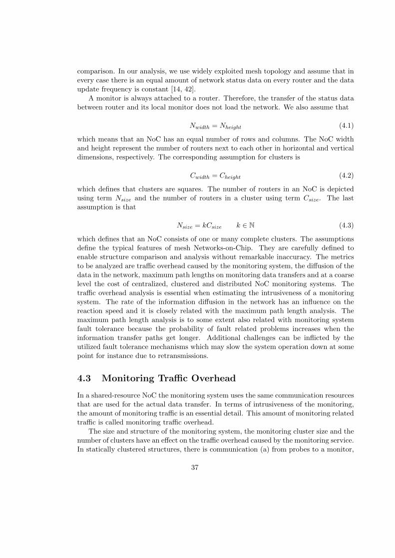
comparison. In our analysis, we use widely exploited mesh topology and assume that inevery case there is an equal amount of network status data on every router and the dataupdate frequency is constant [14, 42].

A monitor is always attached to a router. Therefore, the transfer of the status databetween router and its local monitor does not load the network. We also assume that

Nwidth = Nheight (4.1)

which means that an NoC has an equal number of rows and columns. The NoC widthand height represent the number of routers next to each other in horizontal and verticaldimensions, respectively. The corresponding assumption for clusters is

Cwidth = Cheight (4.2)

which defines that clusters are squares. The number of routers in an NoC is depictedusing term Nsize and the number of routers in a cluster using term Csize. The lastassumption is that

Nsize = kCsize k ∈ N (4.3)

which defines that an NoC consists of one or many complete clusters. The assumptionsdefine the typical features of mesh Networks-on-Chip. They are carefully defined toenable structure comparison and analysis without remarkable inaccuracy. The metricsto be analyzed are traffic overhead caused by the monitoring system, the diffusion of thedata in the network, maximum path lengths on monitoring data transfers and at a coarselevel the cost of centralized, clustered and distributed NoC monitoring systems. Thetraffic overhead analysis is essential when estimating the intrusiveness of a monitoringsystem. The rate of the information diffusion in the network has an influence on thereaction speed and it is closely related with the maximum path length analysis. Themaximum path length analysis is to some extent also related with monitoring systemfault tolerance because the probability of fault related problems increases when theinformation transfer paths get longer. Additional challenges can be inflicted by theutilized fault tolerance mechanisms which may slow the system operation down at somepoint for instance due to retransmissions.

4.3 Monitoring Traffic Overhead

In a shared-resource NoC the monitoring system uses the same communication resourcesthat are used for the actual data transfer. In terms of intrusiveness of the monitoring,the amount of monitoring traffic is an essential detail. This amount of monitoring relatedtraffic is called monitoring traffic overhead.

The size and structure of the monitoring system, the monitoring cluster size and thenumber of clusters have an effect on the traffic overhead caused by the monitoring service.In statically clustered structures, there is communication (a) from probes to a monitor,

37

(b) between monitors and (c) from a monitor to routers. Because the distributed systemcan be seen as a clustered system with the cluster size of 1, there is no communicationinside a cluster, only between them (b). In centralized structures there is only one largecluster which means that the communication is only between probes and monitors (a)as well as between monitors and routers (c) It is assumed that the amount of data on atraffic status update between two network components is so small that a single packetcan hold all the information which is transferred. One transaction in this analysis meansmoving a packet from a router to its neighboring router, from a probe to a monitor orfrom a monitor to a router. The number of transactions required in a complete networkstatus update in a centralized monitoring structure is represented with equation

Tcent = 2Havg

(Nsize − 1

)(4.4)

where Havg is the average hop count between the monitor and any router and Nsize

is the size of the NoC that is the number of routers in the NoC. The multiplier 2depicts bidirectional traffic between the routers and the monitor. The average hop countcan be calculated if a deterministic routing algorithm is used but may vary in systemsusing adaptive routing with non-minimal routes. In a clustered monitoring structurethe number of required transactions in a complete status update is represented withequation

Tclust = 2

(Havg

(Csize − 1

)Nsize

Csize+ Cborders

√Csize

)(4.5)

where the multiplier of 2 illustrates bidirectional traffic in and between clusters. Havg

is the average hop count between any router and the monitor of the same cluster. Nsize

and Csize are sizes of an NoC and a cluster, respectively. Hence, the ratio of these is thenumber of clusters. The first term of the sum represents the traffic inside clusters and thesecond term between the monitors of neighboring clusters. The square root depicts thedistance between the monitors. Cborders is the number of borderlines between clustersand is calculated using equation

Cborders = 2

((√Nsize

Csize− 1

)√Nsize

Csize

)(4.6)

where the second square root represents the number of rows in the network which ismultiplied with the term representing the number of cluster borderlines in a row. Themultiplier of 2 completes the equation to include also the borderlines in the other di-mension, that is horizontal and vertical borderlines. In distributed monitoring structurethere is traffic only between neighboring routers and the number of transactions is cal-culated using equation

Tdist = 4Nsize − 4√Nsize. (4.7)

38

10 20 30 40 50 60 70 80 90 1000

100

200

300

400

500

600

Number of routers

Tra

nsactions

Number of transactions

Centralized

Clustered (25)

Clustered (16)

Clustered (9)

Clustered (4)

Distributed

Clustered (2)

Figure 4.3: Number of transactions required in complete network status update.

The first term of the difference represents the traffic which is sent from each routerin four directions. The second term corrects the amount of traffic in the edges of thenetwork where there is traffic only in two or three directions. Note that Tdist = Tclustwhen Csize = 1 and Tcent = Tclust when Csize = Nsize.

The amount of monitoring communication in NoCs of different sizes and with differ-ent cluster sizes is illustrated in Figure 4.3. The figure shows that larger cluster sizescause more traffic and the centralized system clearly causes the largest traffic overhead.The cluster size of two is also analyzed to complete the analysis. One can notice that itcauses the lowest overhead while the overhead caused by the distributed structure andthe clustered one with the cluster size of four is just slightly higher. However, clusterswith two routers are not well suited to symmetrically structured networks because theyspread the traffic information unevenly.

The lengths of paths between routers, probes and monitors affect the delay of acomplete update process. The comparison of the longest packet transfer paths was madeby calculating the longest productive paths between the possible positions of routersand monitors. A productive path is the shortest routing path between two nodes in anetwork. This comparison is presented in Figure 4.4. The figure shows the longest, or

39

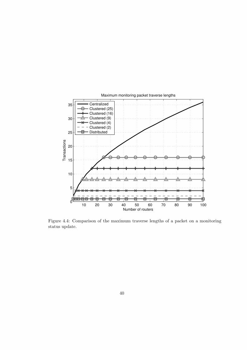
10 20 30 40 50 60 70 80 90 1000

5

10

15

20

25

30

35

Number of routers

Tra

nsa

ctio

ns

Maximum monitoring packet traverse lengths

Centralized

Clustered (25)

Clustered (16)

Clustered (9)

Clustered (4)

Clustered (2)

Distributed

Figure 4.4: Comparison of the maximum traverse lengths of a packet on a monitoringstatus update.

40

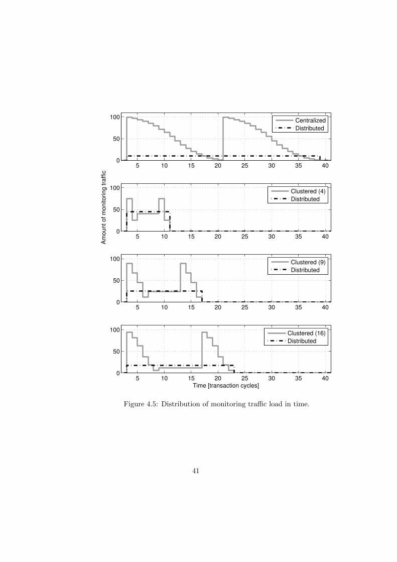
5 10 15 20 25 30 35 400

50

100

Centralized

Distributed

5 10 15 20 25 30 35 400

50

100

Am

ount o

f m

onitorin

g tra

ffic

Clustered (4)

Distributed

5 10 15 20 25 30 35 400

50

100

Clustered (9)

Distributed

5 10 15 20 25 30 35 400

50

100

Time [transaction cycles]

Clustered (16)

Distributed

Figure 4.5: Distribution of monitoring traffic load in time.

41

worst case, distances between routers and monitors or two neighboring monitors (whichone is longer) in different structures. Lengths of the information transfer paths haveto be taken into account because the monitoring data transfer delay has a significantimpact on the monitoring system performance.

The influence of congestion and other problems cannot be seen in this analysis. Ifthe paths of the monitoring packets are significantly rerouted due to problems in thenetwork, the traverse lengths and hop counts can increase. The severity of a problemfor a short path is relatively significant and may completely disable the path. However,the probability of problems is higher for the longer paths and that way the longer thepath, the more vulnerable to faults it is.

One thing to note is how the added monitoring communication overhead is dis-tributed over the time. The amount of monitoring traffic in a network during a completenetwork status data update is presented as a function of time in Figure 4.5. The anal-ysis includes centralized monitoring structure as well as statically clustered structureswith cluster sizes 4, 9 and 16. Each of these structures is separately compared with thedistributed monitoring structure. As can be seen from the Figure 4.5 the load causedby centralized and statically clustered monitoring structures is not only relatively highbut also distributed uneven over time while distributed monitoring systems are able tocause a lot more even load as shown in Figure 4.5. The peaks are caused by varyingdistances between communicating units. At the beginning the amount of traffic is in itsmaximum and it decreases while the data reach the destinations closer to the sender.Two peaks exist because of the bidirectional nature of the traffic. The traffic betweenthese two peaks is the caused by the communication between clusters. However, a dis-

� -SESW

?

6

EN

ES

-�NW NE

6

?

WN

WS

6

-

?

� RouterW

S

E

N

Figure 4.6: Routing directions. The abbreviations stand for N : north, S : south, E : east,W : west and R: router.

42

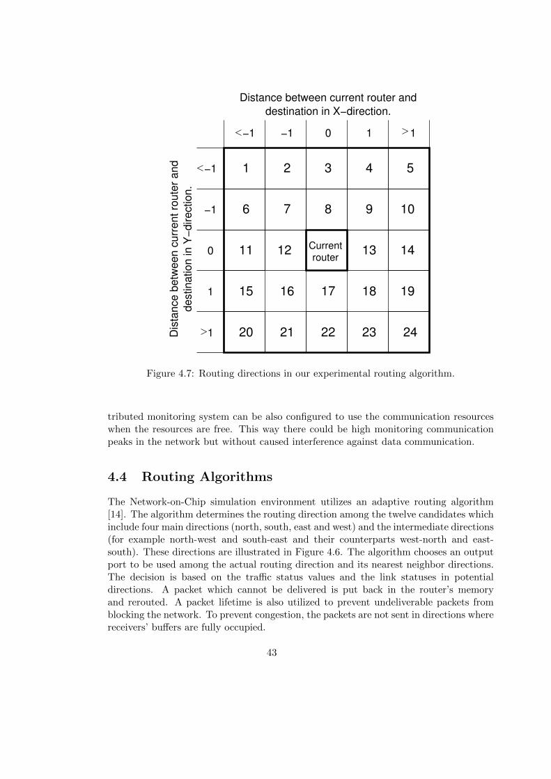
Dis

tan

ce

be

twe

en

cu

rre

nt

rou

ter

an

d

de

stin

atio

n in

Y−

dire

ctio

n.

destination in X−direction.

Distance between current router and

Current

router

0 1−1

1

0

−1 76

1 2 3 4 5

8 9 10

11 12 13 14

15 16 17 18 19

20 21 22 23 24

−1 1

−1

1

Figure 4.7: Routing directions in our experimental routing algorithm.

tributed monitoring system can be also configured to use the communication resourceswhen the resources are free. This way there could be high monitoring communicationpeaks in the network but without caused interference against data communication.

4.4 Routing Algorithms

The Network-on-Chip simulation environment utilizes an adaptive routing algorithm[14]. The algorithm determines the routing direction among the twelve candidates whichinclude four main directions (north, south, east and west) and the intermediate directions(for example north-west and south-east and their counterparts west-north and east-south). These directions are illustrated in Figure 4.6. The algorithm chooses an outputport to be used among the actual routing direction and its nearest neighbor directions.The decision is based on the traffic status values and the link statuses in potentialdirections. A packet which cannot be delivered is put back in the router’s memoryand rerouted. A packet lifetime is also utilized to prevent undeliverable packets fromblocking the network. To prevent congestion, the packets are not sent in directions wherereceivers’ buffers are fully occupied.

43

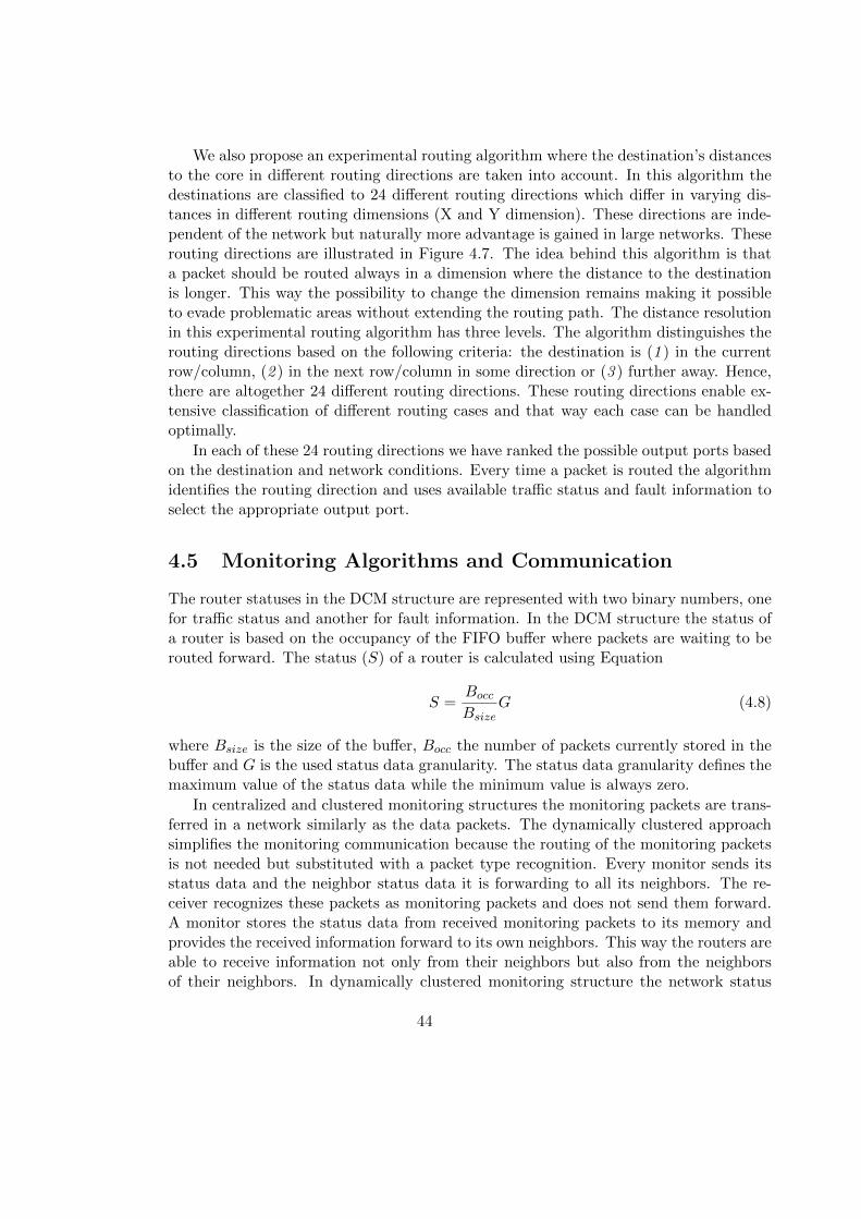
We also propose an experimental routing algorithm where the destination’s distancesto the core in different routing directions are taken into account. In this algorithm thedestinations are classified to 24 different routing directions which differ in varying dis-tances in different routing dimensions (X and Y dimension). These directions are inde-pendent of the network but naturally more advantage is gained in large networks. Theserouting directions are illustrated in Figure 4.7. The idea behind this algorithm is thata packet should be routed always in a dimension where the distance to the destinationis longer. This way the possibility to change the dimension remains making it possibleto evade problematic areas without extending the routing path. The distance resolutionin this experimental routing algorithm has three levels. The algorithm distinguishes therouting directions based on the following criteria: the destination is (1 ) in the currentrow/column, (2 ) in the next row/column in some direction or (3 ) further away. Hence,there are altogether 24 different routing directions. These routing directions enable ex-tensive classification of different routing cases and that way each case can be handledoptimally.

In each of these 24 routing directions we have ranked the possible output ports basedon the destination and network conditions. Every time a packet is routed the algorithmidentifies the routing direction and uses available traffic status and fault information toselect the appropriate output port.

4.5 Monitoring Algorithms and Communication

The router statuses in the DCM structure are represented with two binary numbers, onefor traffic status and another for fault information. In the DCM structure the status ofa router is based on the occupancy of the FIFO buffer where packets are waiting to berouted forward. The status (S) of a router is calculated using Equation

S =Bocc

BsizeG (4.8)

where Bsize is the size of the buffer, Bocc the number of packets currently stored in thebuffer and G is the used status data granularity. The status data granularity defines themaximum value of the status data while the minimum value is always zero.

In centralized and clustered monitoring structures the monitoring packets are trans-ferred in a network similarly as the data packets. The dynamically clustered approachsimplifies the monitoring communication because the routing of the monitoring packetsis not needed but substituted with a packet type recognition. Every monitor sends itsstatus data and the neighbor status data it is forwarding to all its neighbors. The re-ceiver recognizes these packets as monitoring packets and does not send them forward.A monitor stores the status data from received monitoring packets to its memory andprovides the received information forward to its own neighbors. This way the routers areable to receive information not only from their neighbors but also from the neighborsof their neighbors. In dynamically clustered monitoring structure the network status

44

...

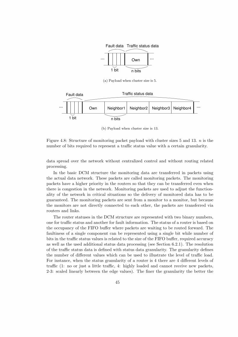
1 bit n bits

...

Traffic status dataFault data

Own

(a) Payload when cluster size is 5.

...

Fault data

1 bit n bits

...

Traffic status data

Neighbor1 Neighbor2 Neighbor3 Neighbor4Own

(b) Payload when cluster size is 13.

Figure 4.8: Structure of monitoring packet payload with cluster sizes 5 and 13. n is thenumber of bits required to represent a traffic status value with a certain granularity.

data spread over the network without centralized control and without routing relatedprocessing.

In the basic DCM structure the monitoring data are transferred in packets usingthe actual data network. These packets are called monitoring packets. The monitoringpackets have a higher priority in the routers so that they can be transferred even whenthere is congestion in the network. Monitoring packets are used to adjust the function-ality of the network in critical situations so the delivery of monitored data has to beguaranteed. The monitoring packets are sent from a monitor to a monitor, but becausethe monitors are not directly connected to each other, the packets are transferred viarouters and links.

The router statuses in the DCM structure are represented with two binary numbers,one for traffic status and another for fault information. The status of a router is based onthe occupancy of the FIFO buffer where packets are waiting to be routed forward. Thefaultiness of a single component can be represented using a single bit while number ofbits in the traffic status values is related to the size of the FIFO buffer, required accuracyas well as the used additional status data processing (see Section 6.2.1). The resolutionof the traffic status data is defined with status data granularity. The granularity definesthe number of different values which can be used to illustrate the level of traffic load.For instance, when the status granularity of a router is 4 there are 4 different levels oftraffic (1: no or just a little traffic, 4: highly loaded and cannot receive new packets,2-3: scaled linearly between the edge values). The finer the granularity the better the

45

accuracy of the status values is.In the DCM structure the monitors exchange their own and their neighbors’ statuses

with each other. Typically monitoring packets include fault statuses of nearby links andone or more traffic statuses of routers depending on the size of the monitoring cluster.The structure of a monitoring packet payload in systems with monitoring cluster sizes5 and 13 is presented in Figure 4.8. The contents of a monitoring packet payload arediscussed in Section 6.2.

In centralized and clustered monitoring structures the monitoring packets are trans-ferred in a network in the same way as the data packets (see Section 4.1). The dynam-ically clustered approach simplifies the monitoring communication because the routingof the monitoring packets is not needed but substituted with a packet type recogni-tion. Every monitor sends its own status data and the neighbor status data, which ithas received from its neighbors, to all other neighbors. The receiver recognizes thesepackets as monitoring packets and does not send them forward. The transfer distanceof a monitoring packet is always one hop, from a router to its neighbor router. Thissimplicity of monitoring packet transferring combined with the simple routing procedureof monitoring packets makes possible to keep the latency overhead on tolerable level formost applications. The presented DCM structure is targeted for applications withoutstrict real-time constraints because the in-time delivery of packets cannot always beguaranteed. This is a trade-off of the improved fault tolerance.

A monitor stores the status data from received monitoring packets to its memoryand provides this information forward to its own neighbors. This way the routers areable to receive information not only from their neighbors but also from the neighborsof their neighbors. In dynamically clustered monitoring structure the network statusdata spread over the network without centralized control and without routing relatedprocessing.

4.6 Summary

This chapter presented the dynamically clustered distributed monitoring structure. Thestructure was analyzed on conceptual level concentrating on the traffic overhead causedby the monitoring system. Routing and monitoring algorithms, which are used with thepresented monitoring structure, were studied and monitoring related communicationdiscussed.

46

Chapter 5

Simulation Environment

SystemC based simulation environment has been implemented to enable extensive anal-ysis of Networks-on-Chip. The simulation environment is required to model and analyzeNetwork-on-Chip (NoC) architectures in terms of functionality, performance and faulttolerance.

SystemC is an extension of C++ programming language [63]. It makes possible tomodel concurrent systems using standard C++ language. The simulation environmentis designed for transaction-level modeling and it utilizes transaction-level modeling li-braries of SystemC (TLM 1.0). [1] Transaction-level simulation environment is suitablefor Network-on-Chip architecture simulations especially in the early phases of systemdevelopment. The environment is easily reconfigurable to model different architecturalsolutions and features without complex immersion to physical implementation for exam-ple using hardware description languages.

The simulation environment includes models of Networks-on-Chip with centralized,clustered and distributed traffic monitoring. In the first phase the simulation environ-ment was designed to model NoCs utilizing shared-resource communication where theresources are shared between the data packets and the monitoring packets. Later theenvironment was further developed to model NoCs with dedicated communication re-sources. These dedicated resources are utilized for serial monitoring communication.

The essence of the simulation environment is the simulation mechanism which isable to execute transient analysis. In transient simulation the cores are sending packetsfollowing a specific traffic pattern and the key figures are recorded during the simulation.These figures include, among others, the numbers of sent and received packets, thetransfer delay and the number of dropped packets from each node separately. Thesimulation duration can be customized and it is possible to run simulation in multipleNoCs simultaneously with identical simulation parameters. In this case, the results canbe represented as averages from the simultaneously running NoCs. The amount of trafficduring the simulation can be adjusted with the traffic pattern. There is also an optionto put faults in the network. This feature enables the fault tolerance analysis of NoC.All the network faults are modeled using the link faults. For instance, a faulty router

47

can be modeled with a bunch of faulty links. Faults can be put in the system randomlyor manually so that modeling of larger uniform fault areas is also possible.

5.1 Architecture

The simulation architecture consists of architectural components and simulator specificcomponents. Architectural components include models of the components which are in-cluded in real NoC implementations: a router, a link, a network interface, a monitor anda core. The core is used to model components which include for instance computationalcores, memories and I/O components. The simulation environment is designed for NoCcommunication infrastructure analysis so the core model includes functionality which isreasonable from the communication point of view.

The simulator specific components do not have physical equivalents but are requiredin the simulation environment. In real implementations a data packet is an abstractconcept but in the simulation environment it is modeled with a standard C++ class.Furthermore, there is terminator components which are used for debugging and misrout-ing detection during simulation.

5.2 Architectural Components

The architectural components of the NoC simulation environment are implemented withSystemC modules (sc module) and the communication between them uses standardSystemC ports (sc port) as well as transaction-level communication defined in TLM1.0. The components and their connections are presented in Figure 5.1 which representsa 2x2 mesh-shaped NoC. The topology and size of the simulated architecture are fullyconfigurable. The structures of the simulator components are presented below. Eachcomponent has operational functions to model the actual run-time behavior, as well asreporting functions to collect the simulation results.

The simulation environment has multiple clocks to control different features. Thereare four independent clocks to control the network components: a core, a router, a linkand a monitor. There are also two slow clocks to control the simulation process: a reportclock (report clk) and a configuration clock (conf clk). These are used to triggersimulation data collection and simulation parameter reconfiguration during simulation.

5.2.1 Router

A router is a network component which forwards traffic in a network. The task of a routeris to direct incoming packets in an appropriate direction. The router has multiple inputand output ports through which it is connected to other routers and cores. Structureof a router was presented in Figure 2.1 on page 6. The three main parts of a routerare switch, routing logic and arbitration logic. The routing logic controls the switch to

48

@@ @@

@@@@

Link

Terminator

Router

NI

Core

Router

RouterRouter

Core Core

CoreM

M M

M

NI NI

NI

Terminator

TerminatorTerminator

Term

inatorTerm

inatorTerminator

Terminator

Figure 5.1: Structure of a 2x2 NoC as modeled in the simulation environment. NIdenotes network interface and M is integrated monitor and probe. In distributed mon-itoring all the monitors are similar, otherwise there are central or cluster monitors andother monitors are simple components which send, receive and store the monitoringinformation.

forward incoming packets to correct output ports and the arbitration logic decides inwhich order the incoming packets are forwarded.

The router model is designed for mesh networks and so it has five ports, four fortraffic to and from the neighboring routers and one for traffic to and from the localcore. The number of ports can be modified. There is a FIFO (first-in-first-out) bufferin each input port and a centralized reroute FIFO for packets which cannot be routedat the first attempt but can be rerouted later. There is also input FIFO buffers forspecial packets: monitoring packets and mapping packets. These special FIFO buffershave implemented to enable packet type prioritization. If the routing fails constantlythe packet is dropped, which means that it is removed from the network and not de-livered to its destination. The router should notify the sender when dropping a packet.However, the reporting feature is not implemented in this simulation environment. Thepacket dropping typically happens in severe situations where routing is inhibited dueto permanently faulty network resources making a destination unreachable. Sizes ofthe FIFO buffers are customizable as well as the packet lifetime before dropping. The

49

Input FIFOs

routing fifo

?

?

?

?

-�- route packet

write

routing arb

Router

do status

packets from network

packets to network

Figure 5.2: Structure of a router including the functions other than the report functions.

router model includes several different routing algorithms. The used algorithm can bechosen with the simulation parameters. The implemented routing algorithms have beendiscussed in Section 4.4.

To enable traffic monitoring there is a traffic monitoring probe whose functionalityis implemented partly in router and monitor components. This probe measures the fillrate of router FIFOs real time, scales the measured value to the used scale and deliversthis scaled value to the local monitor which is optionally attached to the router.

The routing algorithm is defined in the router module in the function route packet.The current implementation utilizes a dimension order routing algorithm which is ableto customize the routing based on the networks status information and link statuses.

The input and output ports for packets are named as target port# and initiator port#

respectively. For monitoring purposes there is

initiator port m and target port m to move monitoring packets between the routerand the local monitor. Input ports link status# and min# are used to transfer neighborlink and router status data from the local monitor to the router. The traffic status of thelocal router is moved to the local monitor through output port mout#. Functions of therouter component are presented below. The functions, other than the report functions,and their relationships are represented in Figure 5.2.

write Write function is executed when a packet is sent to the router through one of thetarget ports. The router identifies the type of the packet. If the packet is a monitoringor a mapping packet, it is stored to the corresponding FIFO. Otherwise the packet isstored in the input FIFO of the port from where the packet arrived. If the correspondingFIFO in any case is fully occupied, the router rejects the incoming packet and the sendercan try to send it to some other router or resend the packet to the current router lateron.

In the system with distributed monitoring, there is a special feature for the monitor-ing packets. Incoming monitoring packets are forwarded straight to the local monitor

50

6

����

���

@@@R

?

-�

@@@I

Router

SSESW

W E

NNW NE

Figure 5.3: Productive routing directions. Letters N, S. E and W denote directionsnorth, south, east and west, correspondingly.

and the packets, sent by the local monitor, are automatically sent to all neighbor routers.

routing arb Routing arbitration function is sensitive to the router clock. The functiontakes packets from the FIFOs and calls the route packet function to route packetsforward. If the routing was successful, the function would remove the packet from theFIFO and increases the processed variable. If the routing failed, the function puts thepacket in the reroute FIFO or if the packet has reached the maximum lifetime (definedwith variable lifetime) the packet is dropped and the variable dropped is incrementedby one. The arbitration algorithm goes through the FIFOs one after another so thatevery FIFO has equal opportunities to get the packets routed forward.

The usage of separate FIFOs for mapping and monitoring packets makes possibleto prioritize these packets over data packets. Reroute FIFO is also prioritized overinput port FIFOs when the reroute FIFO is fully occupied. This is done to prevent theblockage of the router. The simulation environment is configured so that the FIFOs areprioritized in the following order: 1) monitoring packet FIFO, 2) mapping packet FIFO,3) reroute FIFO, 4) input port FIFOs.

route packet The route packet function does the routing decision and tries to sendthe packet to this direction. After the routing the function returns the result of therouting procedure, which are 1) routing succeeded, 2) routing failed, reroute packet and3) routing failed, drop packet. Other results are marks of errors.

In the first phase the function determines the productive directions in x- and y-dimension, which means the direction which leads towards the destination. The routingalgorithm can be also configured to use non-productive directions in problematic situa-tions.

51

� -

6

?

� -

6

?

-�

?

6

1 3

N

E

S

W

2

4

5

6 7

8

9

1011

12

Figure 5.4: Routing directions. Letters N, S. E and W denote directions north, south,east and west, correspondingly.

In the second phase the function defines the routing direction. There is nine possibledirections: local, north, north-east, east, south-east, south, south-west, west and north-west (see Figure 5.3). The intermediate direction (north-east, south-east, etc.) canbe reached through two output ports, in these cases north or east, and south or east,respectively, as shown in Figure 5.4.

In the third phase, the algorithm compares the traffic and link statuses and tries tosend the packet in the direction which it finds the best of the alternatives. The directionoptions are presented in Figure 5.4. Several routing algorithms have been implementedwhich are all based on the basic dimension order routing. The algorithm is selectedusing variable algo. The implemented algorithms include versions of minimal and non-minimal dimension order routing. [14]

do status The do status function calculates the current status of the router. Thestatus is based on the number of packets on the rerouting FIFO, router fifo, but canbe configured to take the other FIFOs in the account too. The status is scaled to theused status granularity scale. The status data granularity is discussed in Section 6.3.1.The current status of a router is calculated using equation

Statusrouter = FifooccGranularity

F ifomax(5.1)

where Fifoocc is the current number of packets in the FIFO buffer or buffers, Granularityis the used status data granularity and Fifomax is the maximum number of packets whichcan be stored to the measured FIFO buffers. This status is sent to the monitor through

52

port mout0.

reset A reset function is implemented to enable the possibility to reset a router duringa simulation. The reset function empties the FIFO buffers.

Reporting Functions Report functions get processed and get dropped are usedto collect statistical data in the end of a simulation. The functions return the totalnumbers of processed and dropped packets during a simulation, respectively. There isalso a FIFO related reporting function get fifosize which returns the number of thepackets which are stored to the router fifo at that moment.

5.2.2 Network Interface

A network interface (NI) is an interface between a core and a router. The purpose of anetwork interface is to wrap the data in packets before sending the data to the networkand unwrap the data from received packets before delivering the data to the local core.

Due to lack of fully functional cores the NI of the simulation environment has onlythe necessary functionality implemented. The component has a write function which isexecuted when a packet is sent to the NI and it directs the packet to the core or to thenetwork. At this point, the simulator does not include specific network interface featuresbut the NIs are combinations of two modules which move the packets to and from thecores. The packet wrapping and unwrapping features can be later added to the NI iffully functional cores are used.

5.2.3 Link

The model of a link in the NoC simulation environment is unidirectional. Links areused in bunches of two in between two routers, one in each direction. The link is asimple component which forwards the incoming packets. A link can be individually setin unusable or faulty state to disable it temporarily or model faults in the network.Unusable and faulty states are similar from the functional point of view. In both statesthe link is disabled and the data are not transferred through the link. A link has avariable direction which shows the direction of a link in the network. When a packetarrives at a link the link calls packet function set sourcedir with its own direction asa parameter. The direction of the previous link on the journey of a packet is stored toa packet to be able to prevent U-turns in routing. The functions and their relationshipsof a link are represented in Figure 5.5.

write Packets are sent to a link by calling the write function. The function storesincoming packets to a FIFO buffer link fifo which is of type queue. The size of theFIFO buffer is parametrized and can be adjusted with the simulation parameters.

53

?

?

?

?

Link

set faultlessset faulty

is faulty

is usableset unusableset usable

link fifo

send packet

write

a routerpackets from

packets toa router

Figure 5.5: Structure of a link including the functions other than the report functions.

send packet A packet sending function is sensitive to the positive clock edge of thelink clock and sends a packet from the link fifo once in a clock cycle to the next router.The delay of a link can be adjusted with the link clock.

Usability and Faultiness Functions A link can be set in faulty or unusable statewhen it cannot be used for data transfer. The link has an built-in model of a link usabilitymonitor so that the usability of the link can be read from port link status. The linkhas functions set faulty, set faultless, set unusable and set usable to modifyusability and faultiness. Usability and faultiness are modeled separately so that a linkcan be set in unusable state temporarily while the faulty state is permanent. When alink is faulty it is always also unusable, but a link can be unusable without being faulty.This has been implemented to be able to separate temporary and permanent unusability.There is also functions is usable and is faulty which return the status of the link.

reset The reset function is sensitive to the configuration clock (conf clk). The func-tion clears the link fifo and puts the link to the usable and faultless state.

5.2.4 Core

Cores are used to model computational cores and memories which are connected to thenetwork through network interfaces and routers. A core sends packets to and receivespackets from the network. Computational features are not modeled in this simulationenvironment but the cores are used to generate traffic which imitates real traffic schemeson a Network-on-Chip. The computational load of a core is modeled using core loadstatus values baseload and additionalload. The computational status of a core iscalculated using equation

CoreLoad = BaseLoad+AdditionalLoad. (5.2)

54

-

?

?

6

generate traffic sendctrl

writeset interval

do status

process loadset additionalloadset baseload

run

Core

packets fromnetwork network

packets to

Figure 5.6: Structure of a core including the functions except the report functions.

The base load models static load while additional load can be changed during the sim-ulation. The core load is utilized especially when task mapping features are simulated.The load values are set using functions set baseload and set additionalload. Afunction process load calculates the total coreload from the base load and additionalload values. A process do status calculates the current core status using equation

CoreStatus = CoreCapacity − CoreLoad. (5.3)

Core capacity is the maximum capacity of a core. In this context it is an abstractconcept which is related to the core load. The core status is delivered to a monitorcomponent for monitoring purposes especially for task mapping. The functions, otherthan the report functions, and their relationships are represented in Figure 5.6. A corehas three different modes to send packets. In the first mode a core sends a data packetto a randomly chosen destination once in a period which is defined with a parameterinterval. The interval is run-time reconfigurable using function set interval. In thesecond mode a core sends multiple packets to a receiving core. The receiver is chosenrandomly and packets are sent to the receiver once in an interval during specific time.The receiver core is selected randomly once in a reconfiguration clock cycle. The twofirst modes can be used together so that a function sendctrl randomly chooses whichmode is used. The third mode is related to the core load modeling. A packet is sentonce in an interval similarly as in the first mode. However, the used interval is based onthe current core load value. The receiver core, which in here is called as a slave core, isset using function set slave. If the third mode is used, the slave core replies to everypacket sending the packet back to the original sender. The remaining functions of thecore component are presented below.

generate traffic Generate traffic function is used to generate destination addressesfor packets which are sent to the network. Variabletraffic pattern defines which traffic pattern is used. The different traffic patternsare presented in Section 5.4.3.

55

run Run function controls the operation of the core module. The function is sensitiveto a positive edge of the core clock. The function generates packets, and depending onthe used mode, defines the destination addresses and sends packets to the network.

write Write function is executed when packets are written from the network to thecore. The function puts the received packet to areceived packets vector, increases the counters of received packets, latency and hops,rec count, total latency, total hops.

Report Functions The core component has several report functions. get hops()

returns a sum of hop counts of all the received packets in a core. Hop count is thenumber of routers which a packet goes through during its route from a sender to areceiver. get latency() returns the sum of transfer latencies of all the received pack-ets. get rec count() returns the number of received packets in a core so the aver-age hop count and latency values can be calculated the results from get hops() andget latency() by dividing them with the result from function get latency(). A func-tion get tried returns the number of packets which have been tried to send from thecore. However, if the network is highly congested the sending could not be possible,the actual number of sent packets is returned by function get sent. The core also hasa function get load which returns the current core load of the core. reset counters

function resets all the statistic values and packet counters.

Mapping Functions The core component includes functions to model task mappingprocess which is presented later in Chapter 7. do mapping function is used to initializetask mapping process. It callssend mapping packet function with desired parameters, generates a mapping packetand sends it to a currently best core in the known neighborhood. The best neighbor isdefined by the monitor component. When a mapping packet is received at a core a func-tion receive mapping packet is executed. The function does a mapping decision, anddepending on the decision, calls functions set additionalload, send mapping packet

or return mapping packet. The return mapping packet function sends the mappingpacket back to the original initiator of the mapping process.

5.2.5 Monitor

The monitors are used to observe the functionality and status of the system. The mon-itor component in our NoC simulation environment includes both a probe to collectthe monitoring data as well as the actual monitor to process the collected data. Themonitor component can be also configured to act only as a probe or a monitor. This isuseful for instance when analyzing centralized monitoring structures [55]. The monitorscommunicate with each other using shared or dedicated resources. The NoC simulationenvironment includes both implementations. When shared resources are used, the mon-itors send packets in the data network. When dedicated resources are used the resources

56

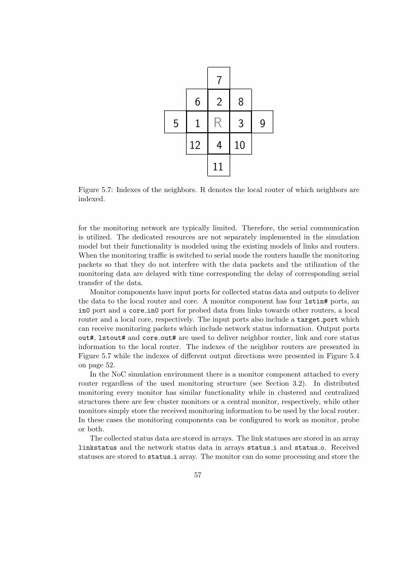
R

12

11

10

95

6 2 8

7

3

4

1

Figure 5.7: Indexes of the neighbors. R denotes the local router of which neighbors areindexed.

for the monitoring network are typically limited. Therefore, the serial communicationis utilized. The dedicated resources are not separately implemented in the simulationmodel but their functionality is modeled using the existing models of links and routers.When the monitoring traffic is switched to serial mode the routers handle the monitoringpackets so that they do not interfere with the data packets and the utilization of themonitoring data are delayed with time corresponding the delay of corresponding serialtransfer of the data.

Monitor components have input ports for collected status data and outputs to deliverthe data to the local router and core. A monitor component has four lstin# ports, anin0 port and a core in0 port for probed data from links towards other routers, a localrouter and a local core, respectively. The input ports also include a target port whichcan receive monitoring packets which include network status information. Output portsout#, lstout# and core out# are used to deliver neighbor router, link and core statusinformation to the local router. The indexes of the neighbor routers are presented inFigure 5.7 while the indexes of different output directions were presented in Figure 5.4on page 52.

In the NoC simulation environment there is a monitor component attached to everyrouter regardless of the used monitoring structure (see Section 3.2). In distributedmonitoring every monitor has similar functionality while in clustered and centralizedstructures there are few cluster monitors or a central monitor, respectively, while othermonitors simply store the received monitoring information to be used by the local router.In these cases the monitoring components can be configured to work as monitor, probeor both.

The collected status data are stored in arrays. The link statuses are stored in an arraylinkstatus and the network status data in arrays status i and status o. Receivedstatuses are stored to status i array. The monitor can do some processing and store the

57

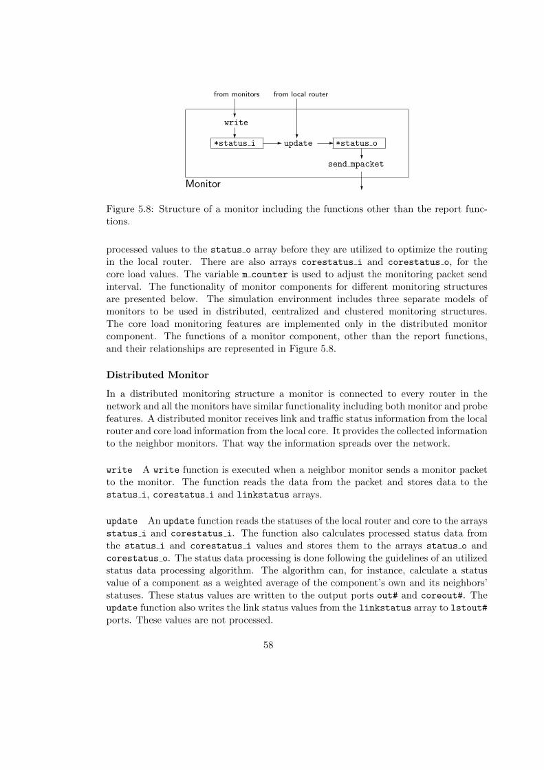
*status i *status o

?

?- -

?

?

?update

send mpacket

write

from local router

Monitor

from monitors

Figure 5.8: Structure of a monitor including the functions other than the report func-tions.

processed values to the status o array before they are utilized to optimize the routingin the local router. There are also arrays corestatus i and corestatus o, for thecore load values. The variable m counter is used to adjust the monitoring packet sendinterval. The functionality of monitor components for different monitoring structuresare presented below. The simulation environment includes three separate models ofmonitors to be used in distributed, centralized and clustered monitoring structures.The core load monitoring features are implemented only in the distributed monitorcomponent. The functions of a monitor component, other than the report functions,and their relationships are represented in Figure 5.8.

Distributed Monitor

In a distributed monitoring structure a monitor is connected to every router in thenetwork and all the monitors have similar functionality including both monitor and probefeatures. A distributed monitor receives link and traffic status information from the localrouter and core load information from the local core. It provides the collected informationto the neighbor monitors. That way the information spreads over the network.

write A write function is executed when a neighbor monitor sends a monitor packetto the monitor. The function reads the data from the packet and stores data to thestatus i, corestatus i and linkstatus arrays.

update An update function reads the statuses of the local router and core to the arraysstatus i and corestatus i. The function also calculates processed status data fromthe status i and corestatus i values and stores them to the arrays status o andcorestatus o. The status data processing is done following the guidelines of an utilizedstatus data processing algorithm. The algorithm can, for instance, calculate a statusvalue of a component as a weighted average of the component’s own and its neighbors’statuses. These status values are written to the output ports out# and coreout#. Theupdate function also writes the link status values from the linkstatus array to lstout#

ports. These values are not processed.

58

send mpacket A send mpacket function generates a monitoring packet once in a statusdata update interval. The length of the interval can be defined as a static duration withthe variable m counter. The length of the interval can be also based on the variationin the status values. The current status value is compared to the previous status valueand to a threshold value. This threshold defines the required difference between currentand previous status until a new monitoring packet is generated and sent. The statusupdate intervals are discussed later in Section 6.1. The send mpacket function storesthe neighbor status data and link status data to the packet and sends it to the routerwhich sends it to all its neighbors.

Report Functions The report functions of a monitor component include get sentmpackets

and reset counters. Former function returns the number of sent monitoring packetsand the latter function resets the monitoring packet counter.

Central Monitor

The central monitor module is used in centralized monitoring structures. There is onecentral monitor in the system where the statuses of all the links and routers are stored.Monitors, which are attached to each router in the network, operate as probes. Theseprobes send their local router’s status to the central monitor which processes the collectedinformation and delivers it to the other routers. Simple probe modules send, receive andstore the monitoring data at the routers but do not do any processing. In the simulationenvironment the central monitor and the probes are modeled using the same monitorcomponent which is configured for different tasks. This operation mode is selected usingvariable textttmode (0: local monitor, 1: central monitor). The address of the centralmonitor is stored to variable m addr in every probe. This is required when sendingobserved status data to the central monitor.

update In the local monitors working as probes the update function reads the currentstatuses from local network components so that they can be sent to the central monitor.In the central monitor mode this function also does the status data processing. Itreads the received raw status data values from the status i array, does the statusdata processing and stores the processed values to the status o array. The status dataprocessing is based on the utilized monitoring algorithm. In both modes the functionalso writes the network and link status data from the arrays to the output ports out#

and lstout#.

send mpacket In the local monitor mode the send mpacket generates a monitoringpacket and stores the traffic status of the local router and the statuses of the outgoinglinks to the packet and sends it to the central monitor. In the central monitor modethis function sends a monitoring packet to a router and its local monitor one afteranother. After the sending the function calculates the address of the next router anduses this address during the following cycle. During every cycle the function takes the

59

corresponding network and link status values from the arrays and does the requiredcalculations before storing them to a packet which is sent to a router.

The functionalities of the write and the report functions are identical to the corre-sponding functions in a distributed monitor.

Cluster Monitor

The cluster monitor is used in clustered monitoring structures. There is a cluster monitorin every cluster and simple monitors attached to all the other routers to send, receiveand store network information. The simple monitors operate as probes. They sendthe statuses from the routers to the cluster monitors which store them, exchange theinformation with other cluster monitors and deliver the data to the simple monitors inits own cluster.

A variable m addr defines the address of the cluster monitor while variables nm#

are used to store the addresses of the cluster monitors of the neighboring clusters.sendingmode variable defines if the monitor is 1) sending monitoring data to the routersin its own cluster or 2) sending monitoring data to the cluster monitors of the neighboringclusters.

update In a local monitor the update function reads the status values from local com-ponents so that they can be sent to the cluster monitor. In the cluster monitor theupdate function works similarly as in the central monitor. When defining the statusesof routers on the borders of the clusters the algorithm takes into account the status ofthe neighbor cluster behind the border. The update function also takes care of puttingstatus data to the output ports out# and lstout# so that they can be read and utilizedby other local components.

write When a monitoring packet is sent to a cluster monitor the write function isexecuted and the network and link status data are written from the packet to the cor-responding variables and arrays in the monitor. The status values of the neighboringclusters are also stored to the status i array.

send mpacket The send mpacket function in a cluster monitor has five different send-ing modes (defined with variable sendingmode). Mode 1 is for sending monitoringpackets to the routers in its own cluster. Modes 2-5 are for sending monitoring packetsto the cluster monitors in the neighboring clusters in west, north, east and south. Inmode 1 the cluster monitor operates similarly as a centralized monitor. In a simple localmonitor the send mpacket function sends the router status and the nearest link statusesto the cluster monitor.

60

5.3 Simulator Components

Simulator components in the simulation environment are not actually implemented onreal Network-on-Chip realizations but necessary to model the system on a simulationenvironment. They can be abstract concepts or components which are implemented fordebugging and monitoring the simulation environment.

5.3.1 Packet

In real implementations a packet is a concept how the data have been structured whenit is transferred in a network. In the simulation environment a packet is a simple C++class which represents the data packets that are moved in the network. Main informationstored in a packet includes source and destination addresses and data payload. Thisinformation is stored in variables source and dest, and data# arrays, respectively.There is also a variable packet type, which indicates the type of the packet. Thetype can be data packet (0), monitoring packet (1), reply packet (2) or mapping packet(3). The reply packets are used when the traffic pattern utilizes automatic replying toreceived packets. The packet type can be read using function get type.

Initialization The initialization function initialize is executed when a packet iscreated. The function sets the current time as the send time of the packet (variablesendtime) and resets the hop count calculator. The hop count calculator counts thetransfer distance of a packet and it is incremented every time the packet is routed bycalling function add hop.

Address Functions Functions get source and get dest return the addresses of thesender and destination of the packet respectively. Every time a packet goes through alink the link sets its direction using function set sourcedir (possible directions: towardsnorth, south, east, or west). A router can read this value using function get sourcedir

when it needs to know from which direction a packet has arrived to a router.

Data Functions The packet can have several arrays which are used to store data(data#). These vectors can be written and read using functions set data# and get data#.

Mapping Functions When a packet is used as a mapping packet, there are specificvariables including variables for caused load, mapper’s address and id, and mappingdistance. The caused load variable represents the size of task which is mapped withthe mapping packet. The unit of the task size is left undefined at this point. Mappingdistance is the distance in hops from the original mapper. A packet includes functionsto read and manipulate these values.

61

Report Functions When a packet arrives at its destination the receiver calls functionset rectime. This function sets the current time as a receiving time of the packet. Thetime of sending and receiving of a packet can be read using functions get sendtime,get rectime. There is also function to read the total latency of a packet, get latency.To read the total hop count of a packet, there is a function get hopcount.

5.3.2 Terminator

A terminator is a component which is implemented only for debug purposes. Terminatorsare connected to the output ports of the routers on the borders of the network so thatpackets which are going outside of the network end to the terminator components. Theterminator is not implemented to real NoC implementations but it can be used detectmisrouted packets in the borders of the network.

5.4 Simulator Functionality

The simulation flow starts from NoC architecture configuration. The simulated Network-on-Chip is structured from separate components which are connected together. Thecomponents are configured with desired parameters and the simulation is started. Afterthe simulation is finished the simulation environment executes result collection functionsand the results are stored for analysis.

The architecture of an NoC is defined in top level class noc. It includes representationof the NoC architecture, its components and how they are connected. The noc class iscontrolled through a main class. All the simulation parameters are defined in the main

class.

5.4.1 Architecture

The noc class generates vectors where the components of the NoC are stored. Thecomponents and the NoC itself are C++ objects. The NoC class connects its componentsto each other. At this time the simulation environment includes only the mesh topologybut the implementation of other topologies is not limited.

The NoC class has functions to generate errors to the system, to control task mappingsimulations and to collect results from the components. For the cases when a staticpacket sending interval is used, there is a function set interval which is sensitive tothe report clock and changes the packet interval based on an interval plan which definesthe intervals used in different phases of the simulation.

generate errors This function generates link faults to the system in random locations.The function puts the chosen links in faulty state so that they are not usable. Therandomization can be overridden so that the faults can be put to certain locationswithout randomization. The number of errors is defined with the variable e in the NoCparameters. The function is sensitive to the reconfiguration clock (conf clk). Each

62

time the generate errors function is executed it resets the links and randomizes newlocations for the link faults in the system.

mapping control This function initiates task mapping process during a simulation.The function is sensitive to the router clock and the designer can choose at which clockcycle a task mapping process is initiated. Two parameters in the process are 1) theaddress of the mapper core and 2) the size of the task.

Reporting Functions The NoC class includes the reporting functions to return keyfigures as total latency, average latency, processed and received packets, packets triedto sent, packets actually sent, sent monitoring packets, total hop count, average hopcount and dropped packets. The statistics are printed out using functions init report

and report. init report is called from inside the report and it calls the report func-tions of the components. The initialization function collects the results from the NoCcomponents and the report function prints them out or saves in a file.

5.4.2 Top Level Control

The top level control of the simulation environment is implemented in main class whichis a mandatory part of every C++ implementation. The class has all the simulationparameters as variables and uses these when creating NoC objects from the noc class.The main class includes a loop where multiple NoCs can be generated with varyingparameters. The top level class initiates the simulation and when it has been completed,collects overall results from the simulated system.

5.4.3 Traffic Pattern

The traffic on a simulated NoC can be based on core load values or a traffic pattern. TheNoC simulation environment has three traffic patterns which are based on randomization.The simplest pattern is a fully random traffic pattern which randomizes the packetdestinations among all the cores in the network. A new destination is randomized forevery sent packet. A weighted random traffic pattern is adjusted so that a one thirdof traffic is between neighboring cores, another third between neighbor’s neighbors andthe last part between all the other cores in the network. This pattern roughly imitatesa traffic pattern in a real NoC implementation where most of the traffic takes placebetween cores near each other.

The third implemented traffic pattern is a two-level pattern which includes uniformrandom traffic and varying hot spots each of which sends a relatively large number ofpackets to a single receiver during a certain time interval. A relatively small numberof cores operate as hot spots simultaneously and send packets to a statically chosenreceiver cores. At the same time, other cores are sending relatively smaller amount oftraffic to random destinations. This two-level traffic pattern imitates real applicationswhere most of the traffic takes place between certain cores at a time. It is aimed for even

63

more realistic performance simulations. The traffic management simulations, presentedin this thesis, are done using this two-level traffic pattern.

5.4.4 Fault Injection

During simulation the network links can be set faulty. In Network-on-Chip simulationsthe fault information can be simplified by using only the information on faulty links andrepresenting other faulty components by marking the links around these components tobe faulty. In the simulation environment the number of faults is defined by the user andthe simulator places the faults randomly in the network. The simulation is executedseveral times with different fault patterns and the results are averaged from the originalsimulation results. This procedure gives overall insight of the operation of the systemwhen parts of the network are faulty.

5.4.5 Task Mapping

To enable run-time task mapping the simulation model of a monitoring packet wasimproved to contain required core load status information and a counter for mappingdecision attempts. The simulation environment is able to report the load of separatecores in any report point (defined by the report clock) during the simulation. It alsoreports the successful task mapping including the IDs of the mapping initiator, assigneeand the number of performed mapping decision attempts.

The simulation environment makes it possible to adjust initial mapping schemes,simulate task mappings and collect results concerning the task mapping processes. Sim-ulation reports include detailed descriptions of each mapping initialization, decision at-tempt and executed mappings. The details include identifiers of the original mapper andthe core where the mapping decision attempt has been carried out. Number of decisionattempts is also presented. The simulation environment is able to illustrate how the coreload is distributed over the system.

5.5 Summary

The SystemC based Network-on-Chip simulation environment was presented in thischapter. The simulation environment includes models of different NoC componentsand it can be configured to simulate features of distinct NoC architectures.

In the following chapters the simulation environment is utilized to model an NoC withthe presented DCM structure (see Chapter 4). In Chapter 6 the simulation environmentis used to model task management features of the DCM structure while in Chapter 7 acase study concerning distributed lightweight task mapping is examined.

The simulation environment is implemented modularly so that in future works itcan be utilized to model Network-on-Chip architectures with new and varying featurescomprehensively.

64

Chapter 6

Traffic Management

The dynamically clustered Network-on-Chip monitoring structure, which was presentedin Chapter 4, is mainly targeted and designed for traffic management purposes. Traf-fic management aims to balance the utilization of network resources so that maximumperformance can be achieved. Essentially, traffic management tries to avoid the develop-ment of highly loaded traffic hot spots in the network. Traffic management should alsokeep the network functioning even though if there are some faulty components. Trafficmanagement related issues are studied in this chapter.

The results presented in this chapter are based on simulations which were carriedout using the simulation environment presented in Chapter 5. Exception to this is thebasic analysis of network status data diffusion in the beginning of Section 6.2 (Figure6.6 on page 75) which is based on conceptual analysis and is carried out similarly as theanalysis presented in Chapter 4.

6.1 Status Update Interval

A status update interval defines how often or in which circumstances a monitor sendsthe updated status data to its neighbors. There are two different approaches: static anddynamic. When a static update interval is used every monitor sends the updated statusdata to its neighbors after a certain time interval regardless of the changes in the dataafter the previous update. The only parameter in the static update is the time betweenthe updates (IntervalStatic). The unit the interval is the minimum time between twosent packets from one source. The time interval parameter should be adjusted in a waythat the network components have up to date status information but the update trafficdoes not strain the communication resources too much.

A dynamic update interval is based on the variation of the status values. The monitorsends the up to date status values to the neighbors when the difference between currentand previous values is more than a pre-defined update threshold (ThresholdDynamic).The unit of the threshold is the same as the unit of the network status values. Thisthreshold is the essential parameter of the dynamic update which is adjusted corre-

65

spondingly as the time interval parameter in the static update procedure. Static anddynamic status update intervals have certain weaknesses. When the network status ischanging rapidly, the static status update misses a fraction of the changes. Surely it canbe configured to be short enough to detect every change but then it would cause futileoverhead during changeless periods. However, after a predefined time interval the statusdata will be exactly up-to-date for a moment. The weaknesses of the dynamic statusupdate interval are opposite to that of the static update interval. When the networkstatus is changing slowly, the status values can be slightly out of date for a relativelylong time before the status value variation reaches the update threshold and will beupdated.

The weaknesses can be compensated by combining these two procedures to an en-hanced dynamic status update interval. This interval type has two parameters whichare familiar from the static and dynamic intervals: time interval (IntervalEnhanced) andthreshold (ThresholdEnhanced). This method works similarly as the dynamic status up-date interval but there is also a time interval parameter which defines the maximum

0 0.1 0.2 0.3 0.4 0.5 0.6 0.7 0.8 0.9 10

0.02

0.04

0.06

0.08

0.1

0.12

0.14

0.16

0.18

0.2

Sent packets [fraction of capacity]

De

live

red

pa

cke

ts [

fra

tio

n o

f ca

pa

city]

Throughput, no faults

Static

Dynamic

Enhanced

No monitoring

Figure 6.1: Throughput with different status update interval procedures and iden-tical traffic pattern. No faults. IntervalStatic = 23, ThresholdDynamic = 3,IntervalEnhanced = 50, ThresholdEnhanced = 5

66

time between two status updates regardless of the variation of these values. When theenhanced dynamic status update interval is used, larger threshold and time interval pa-rameters can be applied than in static or a dynamic update interval. This can be usedto decrease the number of monitoring packets while performance is improved.

6.1.1 Status Update Interval Analysis

The influence of the different status update intervals on the network throughput werecompared. Figure 6.1 and Figure 6.2 present the throughput of a 64-router NoC withstatic, dynamic and enhanced dynamic status update interval protocols in faultless net-work and when 10% of links in the network are faulty, respectively. The throughput ofa corresponding NoC without monitoring and routing adaptivity is also presented. Theupdate interval parameters are adjusted so that the numbers of sent monitoring packetsduring the simulations are at the same range with each other. Status data granularityis 32 which means that the network status values are in range of 0–31.

0 0.1 0.2 0.3 0.4 0.5 0.6 0.7 0.8 0.9 10

0.02

0.04

0.06

0.08

0.1

0.12

0.14

0.16

0.18

0.2

Sent packets [fraction of capacity]

De

live

red

pa

cke

ts [

fra

tio

n o

f ca

pa

city]

Throughput, 10% of links faulty

Static

Dynamic

Enhanced

No monitoring

Figure 6.2: Throughput with different status update interval procedures and identicaltraffic pattern. 10% of the links are faulty. IntervalStatic = 23, ThresholdDynamic = 3,IntervalEnhanced = 50, ThresholdEnhanced = 5

67

The obtained performance values with different status update intervals were com-pared in a point where the throughput has been saturated. The point, where 60% ofthe maximum capacity of packets were sent during a routing cycle, was used for themeasurements. As can be seen in Figure 6.1 and Figure 6.2, the dynamic and enhanceddynamic update intervals improve network performance significantly while the improve-ment with the static status update interval is slightly lower. In a faultless network thestatic interval causes 21% improvement when compared to a system without any mon-itoring. At the same time the dynamic and the enhanced update intervals reach 29%performance improvement. In a faulty network the throughput increase of 70% has beenreached using the dynamic and the enhanced dynamic status update intervals. Thecorresponding performance improvement with the static update interval is 63%. Theseproposed methods make it possible to gain major improvements in the overall perfor-mance especially when parts of the network resources are faulty or unusable. When theresults from the faultless and the faulty network are compared, one can note that in thesystem without monitoring the performance drops 40% when faults are added to thenetwork. The corresponding drop when monitoring with static update interval is used

0.1 0.2 0.3 0.4 0.5 0.6 0.7 0.8 0.9 10

0.02

0.04

0.06

0.08

0.1

0.12

0.14

0.16

0.18

0.2

Sent data packets [fraction of capacity]

Se

nt

mo

nito

rin

g p

acke

ts [

fra

tio

n o

f ca

pa

city]

Sent monitoring packets, no faults

Static

Dynamic

Enhanced

Figure 6.3: Number of sent monitoring packets. No faults. IntervalStatic = 23,ThresholdDynamic = 3, IntervalEnhanced = 50, ThresholdEnhanced = 5

68

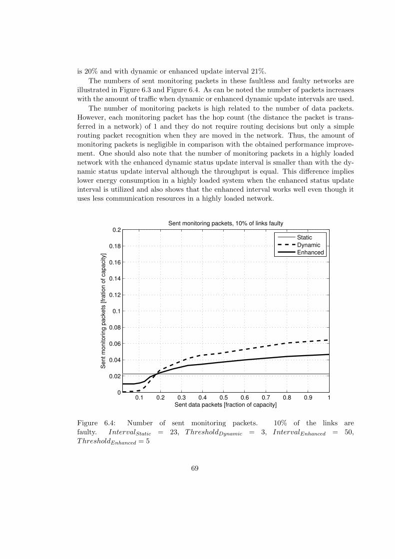
is 20% and with dynamic or enhanced update interval 21%.

The numbers of sent monitoring packets in these faultless and faulty networks areillustrated in Figure 6.3 and Figure 6.4. As can be noted the number of packets increaseswith the amount of traffic when dynamic or enhanced dynamic update intervals are used.

The number of monitoring packets is high related to the number of data packets.However, each monitoring packet has the hop count (the distance the packet is trans-ferred in a network) of 1 and they do not require routing decisions but only a simplerouting packet recognition when they are moved in the network. Thus, the amount ofmonitoring packets is negligible in comparison with the obtained performance improve-ment. One should also note that the number of monitoring packets in a highly loadednetwork with the enhanced dynamic status update interval is smaller than with the dy-namic status update interval although the throughput is equal. This difference implieslower energy consumption in a highly loaded system when the enhanced status updateinterval is utilized and also shows that the enhanced interval works well even though ituses less communication resources in a highly loaded network.

0.1 0.2 0.3 0.4 0.5 0.6 0.7 0.8 0.9 10

0.02

0.04

0.06

0.08

0.1

0.12

0.14

0.16

0.18

0.2

Sent data packets [fraction of capacity]

Se

nt

mo

nito

rin

g p

acke

ts [

fra

tio

n o

f ca

pa

city]

Sent monitoring packets, 10% of links faulty

Static

Dynamic

Enhanced

Figure 6.4: Number of sent monitoring packets. 10% of the links arefaulty. IntervalStatic = 23, ThresholdDynamic = 3, IntervalEnhanced = 50,ThresholdEnhanced = 5

69

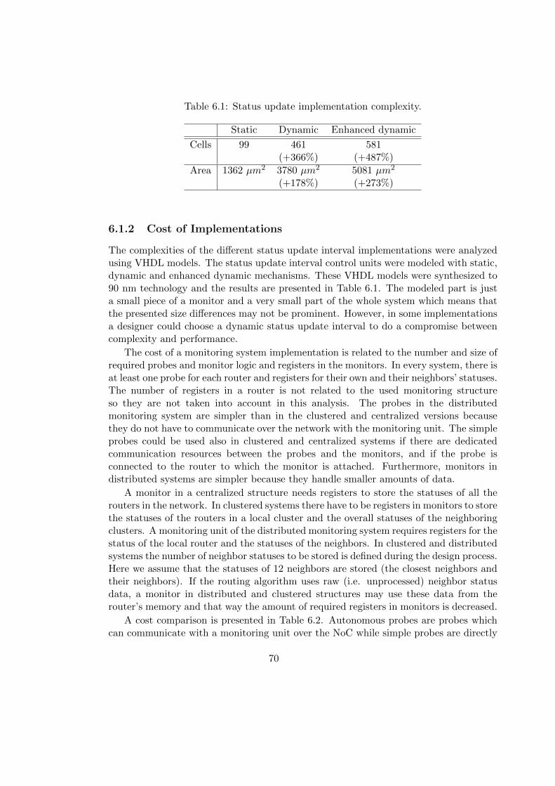
Table 6.1: Status update implementation complexity.

Static Dynamic Enhanced dynamic

Cells 99 461 581(+366%) (+487%)

Area 1362 µm2 3780 µm2 5081 µm2

(+178%) (+273%)

6.1.2 Cost of Implementations

The complexities of the different status update interval implementations were analyzedusing VHDL models. The status update interval control units were modeled with static,dynamic and enhanced dynamic mechanisms. These VHDL models were synthesized to90 nm technology and the results are presented in Table 6.1. The modeled part is justa small piece of a monitor and a very small part of the whole system which means thatthe presented size differences may not be prominent. However, in some implementationsa designer could choose a dynamic status update interval to do a compromise betweencomplexity and performance.

The cost of a monitoring system implementation is related to the number and size ofrequired probes and monitor logic and registers in the monitors. In every system, there isat least one probe for each router and registers for their own and their neighbors’ statuses.The number of registers in a router is not related to the used monitoring structureso they are not taken into account in this analysis. The probes in the distributedmonitoring system are simpler than in the clustered and centralized versions becausethey do not have to communicate over the network with the monitoring unit. The simpleprobes could be used also in clustered and centralized systems if there are dedicatedcommunication resources between the probes and the monitors, and if the probe isconnected to the router to which the monitor is attached. Furthermore, monitors indistributed systems are simpler because they handle smaller amounts of data.

A monitor in a centralized structure needs registers to store the statuses of all therouters in the network. In clustered systems there have to be registers in monitors to storethe statuses of the routers in a local cluster and the overall statuses of the neighboringclusters. A monitoring unit of the distributed monitoring system requires registers for thestatus of the local router and the statuses of the neighbors. In clustered and distributedsystems the number of neighbor statuses to be stored is defined during the design process.Here we assume that the statuses of 12 neighbors are stored (the closest neighbors andtheir neighbors). If the routing algorithm uses raw (i.e. unprocessed) neighbor statusdata, a monitor in distributed and clustered structures may use these data from therouter’s memory and that way the amount of required registers in monitors is decreased.

A cost comparison is presented in Table 6.2. Autonomous probes are probes whichcan communicate with a monitoring unit over the NoC while simple probes are directly

70

Table 6.2: Monitoring system cost comparison.

Distributed Clustered Centralized

Autonomous probes 0 n− dn/me n− 1Simple probes n dn/me 1

Cluster monitors 0 dn/me 1Simple monitors n 0 0

Registers in a monitor 1 . . . (q + 1) m. . . (m+ q) n

n = routers in the network

m = routers in a cluster

q = neighboring monitors/clusters whose overall statuses are stored in a monitor

connected to a monitor with dedicated communication resources. Cluster monitors aremonitors that take care of several probes and routers. Those are used in centralizedand clustered systems while simple monitors, which just take care of a single probeand communicate with their neighboring monitors, are used in distributed monitoringsystems. The required amount of memory in the monitors is defined as the numberof registers where one register is able to store the status of one router. The numberof required registers is listed on the table. The number of registers in distributed andclustered structures depends on how efficiently the registers of the local router can beutilized for the purposes of the monitor.

Exact cost comparison is impossible without circuit implementations but some esti-mations of the component sizes and especially of their mutual ratios can be made. Atfirst we define the units; the size of a simple probe: SP , and the unit cost for monitors:SM . An autonomous probe is a simple probe with capability to communicate over anNoC. The probe and the communication part of a probe are assumed to be roughly thesame size which leads to an assumption that the size of an autonomous probe is 2SP . An-other assumption is the ratio of the different monitor sizes. The approximated monitorsizes are related to the number of direct connections from a monitor to probes, routersand other monitors. SM is equivalent to the cost of logic required for one connection,for instance the size of a monitor in the middle of a distributed monitoring system is6SM because the monitor is connected to a probe, a router and four neighbor monitors.In addition we denote the size of a register with SR.

By using the above assumptions, we can carry out a cost comparison of monitoringsystems for an NoC with 100 routers (Table 6.3). Note that there are no assumptions onthe relations between units SP , SM and SR which means that they are not comparablewith each other.

The approximations in Table 6.3 show that the distributed implementation is theleast complex in terms of probes. The number of registers depends on the used moni-

71

Table 6.3: Cost of 100-router NoC with different monitoring structures.

Distributed Centralized

Probes 100SP 199SPMonitors 560SM 200SMRegisters 100SR...1096SR 100SR

Clustered (4) Clustered (16) Clustered (25)

Probes 175SP 191SP 196SPMonitors 280SM 224SM 208SMRegisters 100SR...284SR 100SR...152SR 100SR...112SR

Size of a cluster in parentheses.

toring algorithm but is at least equal to the number of routers and increases when thesize of a cluster decreases. The analysis shows that when using distributed monitoringstructure it is strongly recommended to integrate the router and the monitor and sharethe status registers among them. This can be done also when the cluster size is rela-tively small and raw monitoring data are stored to the status registers of the routers. Inlarge clusters, the neighbor cluster statuses are stored to the routers far away from themonitor, which makes the register sharing difficult. Table 6.3 also shows that the totalcost of monitors decreases when the size of a cluster increases.

It has to be noted that in distributed implementations the computation is done insmaller parts by simple components working at the same speed with the larger monitors.That way the distributed system may reach significantly higher performance because theamount of data to be processed in a monitor is substantially smaller, or they can be op-timized for low power consumption and area. Furthermore, the distributed monitoringsystem can be more fault tolerant because the computation is divided into the smallmonitoring units and each of them is much less critical in terms of overall system func-tionality than the larger monitors in clustered and centralized systems.

6.2 Status Data Diffusion

The network status data diffusion defines how far the status of a network component (inour analysis router) spreads in the network. A wider diffusion area makes it possible toreact to problems early and avoid routing packets to the worst hot spots or faulty areas.

Network information diffusion in distributed and statically clustered network mon-itoring is illustrated in Figure 6.5. Diffusion of information in a monitoring system isdivided into phases so that a phase consists of traffic information collection inside a

72

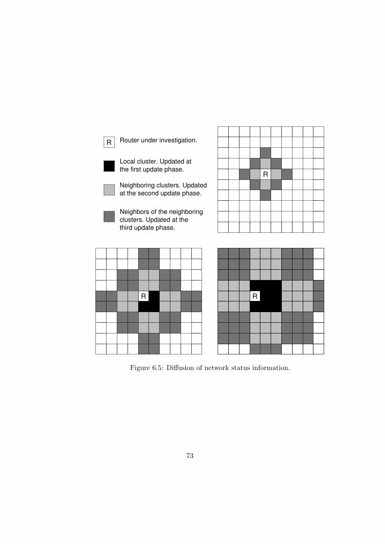
R

R

R R

Router under investigation.

Local cluster. Updated at

the first update phase.

Neighboring clusters. Updated

at the second update phase.

Neighbors of the neighboring

clusters. Updated at the

third update phase.

Figure 6.5: Diffusion of network status information.

73

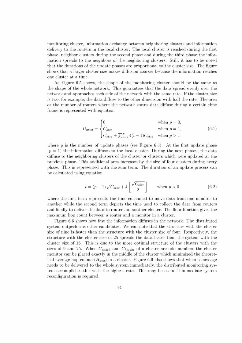
monitoring cluster, information exchange between neighboring clusters and informationdelivery to the routers in the local cluster. The local cluster is reached during the firstphase, neighbor clusters during the second phase and during the third phase the infor-mation spreads to the neighbors of the neighboring clusters. Still, it has to be notedthat the durations of the update phases are proportional to the cluster size. The figureshows that a larger cluster size makes diffusion coarser because the information reachesone cluster at a time.

As Figure 6.5 shows, the shape of the monitoring cluster should be the same asthe shape of the whole network. This guarantees that the data spread evenly over thenetwork and approaches each side of the network with the same rate. If the cluster sizeis two, for example, the data diffuse to the other dimension with half the rate. The areaor the number of routers where the network status data diffuse during a certain timeframe is represented with equation

Darea =

0 when p = 0,

Csize when p = 1,

Csize +∑p

i=2 4(i− 1)Csize when p > 1

(6.1)

where p is the number of update phases (see Figure 6.5). At the first update phase(p = 1) the information diffuses to the local cluster. During the next phases, the datadiffuse to the neighboring clusters of the cluster or clusters which were updated at theprevious phase. This additional area increases by the size of four clusters during everyphase. This is represented with the sum term. The duration of an update process canbe calculated using equation

t = (p− 1)√Csize + 4

⌊√Csize

2

⌋when p > 0 (6.2)

where the first term represents the time consumed to move data from one monitor toanother while the second term depicts the time used to collect the data from routersand finally to deliver the data to routers on another cluster. The floor function gives themaximum hop count between a router and a monitor in a cluster.

Figure 6.6 shows how fast the information diffuses in the network. The distributedsystem outperforms other candidates. We can note that the structure with the clustersize of nine is faster than the structure with the cluster size of four. Respectively, thestructure with the cluster size of 25 spreads the data faster than the system with thecluster size of 16. This is due to the more optimal structure of the clusters with thesizes of 9 and 25. When Cwidth and Cheight of a cluster are odd numbers the clustermonitor can be placed exactly in the middle of the cluster which minimized the theoret-ical average hop counts (Havg) in a cluster. Figure 6.6 also shows that when a messageneeds to be delivered to the whole system immediately, the distributed monitoring sys-tem accomplishes this with the highest rate. This may be useful if immediate systemreconfiguration is required.

74

0 5 10 15 20 25 300

100

200

300

400

500

600

700

800

900

1000

Time [transaction cycles]

Diffu

sio

n [ro

ute

rs]

Diffusion of status information

Distributed

Clustered (4)

Clustered (9)

Clustered (16)

Clustered (25)

Figure 6.6: Diffusion of network status information as a function of time (size of a clusterin parentheses).

There are two factors which affect the status data diffusion: the size of a dynamiccluster and status data processing. The cluster size defines how far the status data diffusefrom a router and the amount of neighbor status data a router has. The cluster size hasan effect on the quantity of neighbor status data to be transferred in a monitoring packet.If the size of a dynamic cluster is 5, it contains the neighbors of a router and the routeritself. In this case it is enough to send only the router’s own status to the neighbors.If the size of a cluster is 13, it also includes the neighbors of the neighbors and thenfour neighbor statuses should be included in every monitoring packet. In larger dynamicclusters the amount of monitoring data which has to be included in a monitoring packetincreases to a level which is not practical. Therefore, we have limited our analysis to thedynamic cluster sizes of 5 and 13.

6.2.1 Additional Status Data Processing

In DCM structure the network traffic status values are based on the load of the routers.When additional status data processing is used, each router status value is based on

75

� -SESW

?

6

EN

ES

-�NW NE

6

?

WN

WS

6

-

?

� RouterW

S

E

N

Figure 6.7: Routing directions. The abbreviations N, S, E and W stand for directionsnorth, south, east and west, correspondingly.

the state of the router itself and the state of its neighbors. When the neighbor routers’status is defined using also its own neighbors, the status data diffuse over the network.

A processed status of a router (S), which represents the traffic load in a router andits surroundings, is calculated using Equation 6.3 where Sx, x ∈ {L,N, S,E,W} is thestatus of a neighboring router in a specific direction (Local router, or a neighbor inN orth, South, East or W est direction).

S = αSL +1− α

4(SN + SS + SE + SW ) (6.3)

where α is a factor which defines which part of the router status is related to its ownutilization level. When the status data of twelve neighbors is used the statuses of differentrouting directions are calculated using for example Equation 6.5 and Equation 6.6, where

Dx, x ∈ {N,S,E,W,NW,WN,NE,EN, SW,WS, SE,ES}, (6.4)

represents the status of a routing direction and Ni where 1 ≤ i ≤ CSize− 1 is the statusof a neighboring router in a specific index. Other ten statuses are calculated usingcorresponding equations. The routing directions are represented in Figure 6.7 and theused indexes of the neighbor routers in Figure 6.8.

DN = βN2 + (1− β)N7 (6.5)

DES = γN3 +1− γ

2(N9 +N10) (6.6)

76

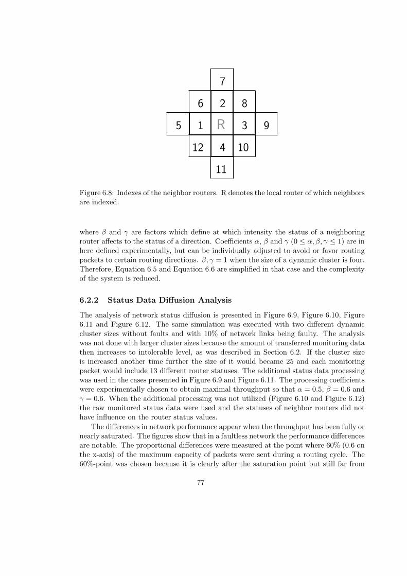
R

12

11

10

95

6 2 8

7

3

4

1

Figure 6.8: Indexes of the neighbor routers. R denotes the local router of which neighborsare indexed.

where β and γ are factors which define at which intensity the status of a neighboringrouter affects to the status of a direction. Coefficients α, β and γ (0 ≤ α, β, γ ≤ 1) are inhere defined experimentally, but can be individually adjusted to avoid or favor routingpackets to certain routing directions. β, γ = 1 when the size of a dynamic cluster is four.Therefore, Equation 6.5 and Equation 6.6 are simplified in that case and the complexityof the system is reduced.

6.2.2 Status Data Diffusion Analysis

The analysis of network status diffusion is presented in Figure 6.9, Figure 6.10, Figure6.11 and Figure 6.12. The same simulation was executed with two different dynamiccluster sizes without faults and with 10% of network links being faulty. The analysiswas not done with larger cluster sizes because the amount of transferred monitoring datathen increases to intolerable level, as was described in Section 6.2. If the cluster sizeis increased another time further the size of it would became 25 and each monitoringpacket would include 13 different router statuses. The additional status data processingwas used in the cases presented in Figure 6.9 and Figure 6.11. The processing coefficientswere experimentally chosen to obtain maximal throughput so that α = 0.5, β = 0.6 andγ = 0.6. When the additional processing was not utilized (Figure 6.10 and Figure 6.12)the raw monitored status data were used and the statuses of neighbor routers did nothave influence on the router status values.

The differences in network performance appear when the throughput has been fully ornearly saturated. The figures show that in a faultless network the performance differencesare notable. The proportional differences were measured at the point where 60% (0.6 onthe x-axis) of the maximum capacity of packets were sent during a routing cycle. The60%-point was chosen because it is clearly after the saturation point but still far from

77

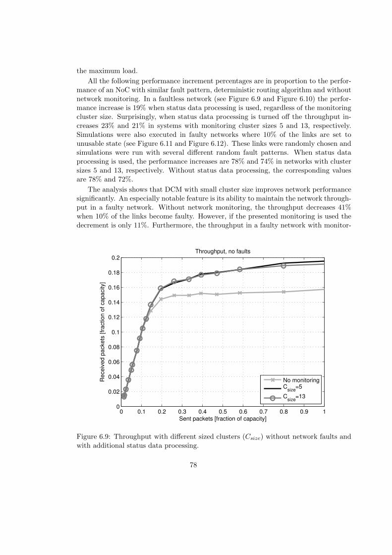
the maximum load.

All the following performance increment percentages are in proportion to the perfor-mance of an NoC with similar fault pattern, deterministic routing algorithm and withoutnetwork monitoring. In a faultless network (see Figure 6.9 and Figure 6.10) the perfor-mance increase is 19% when status data processing is used, regardless of the monitoringcluster size. Surprisingly, when status data processing is turned off the throughput in-creases 23% and 21% in systems with monitoring cluster sizes 5 and 13, respectively.Simulations were also executed in faulty networks where 10% of the links are set tounusable state (see Figure 6.11 and Figure 6.12). These links were randomly chosen andsimulations were run with several different random fault patterns. When status dataprocessing is used, the performance increases are 78% and 74% in networks with clustersizes 5 and 13, respectively. Without status data processing, the corresponding valuesare 78% and 72%.

The analysis shows that DCM with small cluster size improves network performancesignificantly. An especially notable feature is its ability to maintain the network through-put in a faulty network. Without network monitoring, the throughput decreases 41%when 10% of the links become faulty. However, if the presented monitoring is used thedecrement is only 11%. Furthermore, the throughput in a faulty network with monitor-

0 0.1 0.2 0.3 0.4 0.5 0.6 0.7 0.8 0.9 10

0.02

0.04

0.06

0.08

0.1

0.12

0.14

0.16

0.18

0.2

Sent packets [fraction of capacity]

Receiv

ed p

ackets

[fr

action o

f capacity]

Throughput, no faults

No monitoringC

size=5

Csize

=13

Figure 6.9: Throughput with different sized clusters (Csize) without network faults andwith additional status data processing.

78

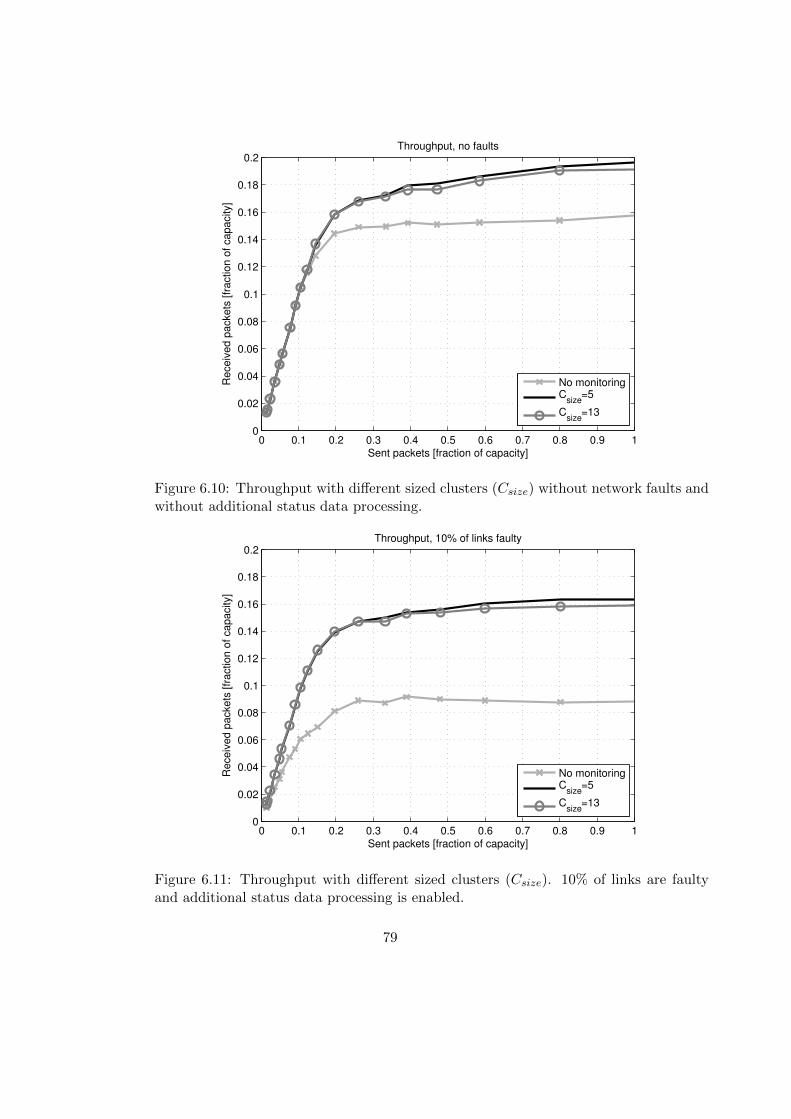
0 0.1 0.2 0.3 0.4 0.5 0.6 0.7 0.8 0.9 10

0.02

0.04

0.06

0.08

0.1

0.12

0.14

0.16

0.18

0.2

Sent packets [fraction of capacity]

Re

ce

ive

d p

acke

ts [

fra

ctio

n o

f ca

pa

city]

Throughput, no faults

No monitoringC

size=5

Csize

=13

Figure 6.10: Throughput with different sized clusters (Csize) without network faults andwithout additional status data processing.

0 0.1 0.2 0.3 0.4 0.5 0.6 0.7 0.8 0.9 10

0.02

0.04

0.06

0.08

0.1

0.12

0.14

0.16

0.18

0.2

Sent packets [fraction of capacity]

Re

ce

ive

d p

acke

ts [

fra

ctio

n o

f ca

pa

city]

Throughput, 10% of links faulty

No monitoringC

size=5

Csize

=13

Figure 6.11: Throughput with different sized clusters (Csize). 10% of links are faultyand additional status data processing is enabled.

79

ing is 6% higher than it of a faultless network without monitoring.

A noteworthy observation is that a larger cluster size does not have positive impacton the performance but actually reduces it. This phenomenon can have multiple reasons.One reason for the inefficiency can be that too much data processing leads to inaccuratestatus data. The network status values are based on the status of the current routeras well as the statuses of its neighbor routers. Too much of averaging between thestatus values equalizes the status values over the network and dissolves the differencesbetween them. Another reason could be the latency in the status data propagation whichmakes it outdated before it is utilized. The monitored status data are transferred usingthe shared network resources in the actual data network. Even though the monitoringdata are prioritized and passes all the other data in the router buffers, the transferlatency especially between the current router and the neighbors of the neighbors ispresent. When the traffic pattern in the network is rapidly changing the network withlarge monitoring cluster size possibly cannot react to the change quick enough. A largecluster could work in networks with more static traffic pattern. However, the needfor routing reconfiguration and extensive network monitoring is lower in these kind ofsystems. Therefore, rapid reacting to change in the traffic pattern is necessary.

The influence of the additional status data processing is small or even non-existent.

0 0.1 0.2 0.3 0.4 0.5 0.6 0.7 0.8 0.9 10

0.02

0.04

0.06

0.08

0.1

0.12

0.14

0.16

0.18

0.2

Sent packets [fraction of capacity]

Receiv

ed p

ackets

[fr

action o

f capacity]

Throughput, 10% of links faulty

No monitoringC

size=5

Csize

=13

Figure 6.12: Throughput with different sized clusters (Csize). 10% of links are faultyand additional status data processing is disabled.

80

0 0.1 0.2 0.3 0.4 0.5 0.6 0.7 0.8 0.9 10

0.02

0.04

0.06

0.08

0.1

0.12

0.14

0.16

0.18

0.2

Sent packets [fraction of capacity]

Receiv

ed p

ackets

[fr

action o

f capacity]

Throughput, 10% of links faulty

With processing

Without processing

Figure 6.13: Throughput with and without additional status data processing. Csize = 5,10% of links are faulty.

In a faulty network there is a very small increase in the throughput. However, in afaultless network the impact is even negative. For example, Figure 6.13 shows thedifference in throughput in a faulty network with CSize = 5. As can be seen in thisspecific comparison the difference is negligible.

The inefficiency of the status data processing may stem from the same factors asthat of the large cluster size. The differences between status values dissolve and are noton display so that the routing algorithm could make right decisions.

6.3 Format of Network Status Data

The network status data are used to deliver the information of the state of the networkand it can be used to different purposes. When the main purpose of use is trafficmanagement the data typically include information concerning network load and faults.Faults are simply denoted using binary values which indicate if a component of thenetwork is usable or faulty. In more complex systems multi-level fault indicators couldbe considered. The network load is denoted using a scale where different values representdifferent amounts of load on a network component. In our simulations, the network load

81

representation is linear. Different scales can be considered in some specific applications.

6.3.1 Granularity of the Router Status Values

The status data granularity defines the resolution of the status data values which ishow many different values there are on the scale which is used to represent the loadon a network component. The smallest used value indicates that the load of a networkcomponent is very low and the highest value represents a high load of the component.The rest of the values indicate component load linearly between the extreme values. Anexample of the status data granularity was given in Section 4.5. In physical implementa-tions, the status data values are represented as binary numbers which means that finergranularity requires more bits and that way increases the size of monitoring packet pay-load. The status data granularity impacts on to the amount of the monitoring data tobe transferred as well as to the required computational resources in the monitoring com-ponents. The granularity should be chosen so that the required data transfer and statusdata processing resources are adequate in the framework of the NoC implementation inquestion.

The 64-core NoC has been simulated with different granularity alternatives. 32 wasdefined to the maximum possible granularity because of the limited size of payload inthe monitoring packets. A status value with 32-level granularity can be indicated with 5bits. When monitoring cluster size is 13 a monitoring packet should include informationon router’s status and statuses of its four neighbors. With the granularity of 32, thistakes 25 bits which can be considered a realistic amount of data in a monitoring packet.The same data granularity is also used between probes and monitors.

The throughput of a 64-core NoC with diverse status granularity is presented inFigure 6.14, Figure 6.15, Figure 6.16 and Figure 6.17. The simulations were carriedout in a faultless network and in a network where 10% of the links were faulty. Theresults show that in a fully functional network the performance is only slightly improvedwhen granularity is larger than eight. It can be also noted that in a faulty network thegranularity should be at least 16. In both cases 4-level granularity leads to significantlylower performance which means 7% decrement in the faultless and 4% in the faultynetwork compared with the 16-level granularity. This supports the use of at least 16-level granularity. The performance of the system without monitoring is illustrated as areference.

6.3.2 Combining Router and Link Statuses

Unification of traffic and fault information is a method to simplify monitoring statusdata. In the original status data format (see Figure 4.8) there is a binary number torepresent the traffic load and a bit to indicate the resource faultiness. To decreasethe monitoring complexity and the size of monitoring data payload we analyzed twoapproaches where the monitoring data are combined to hybrid forms. These two hybriddata formats are presented below.

82

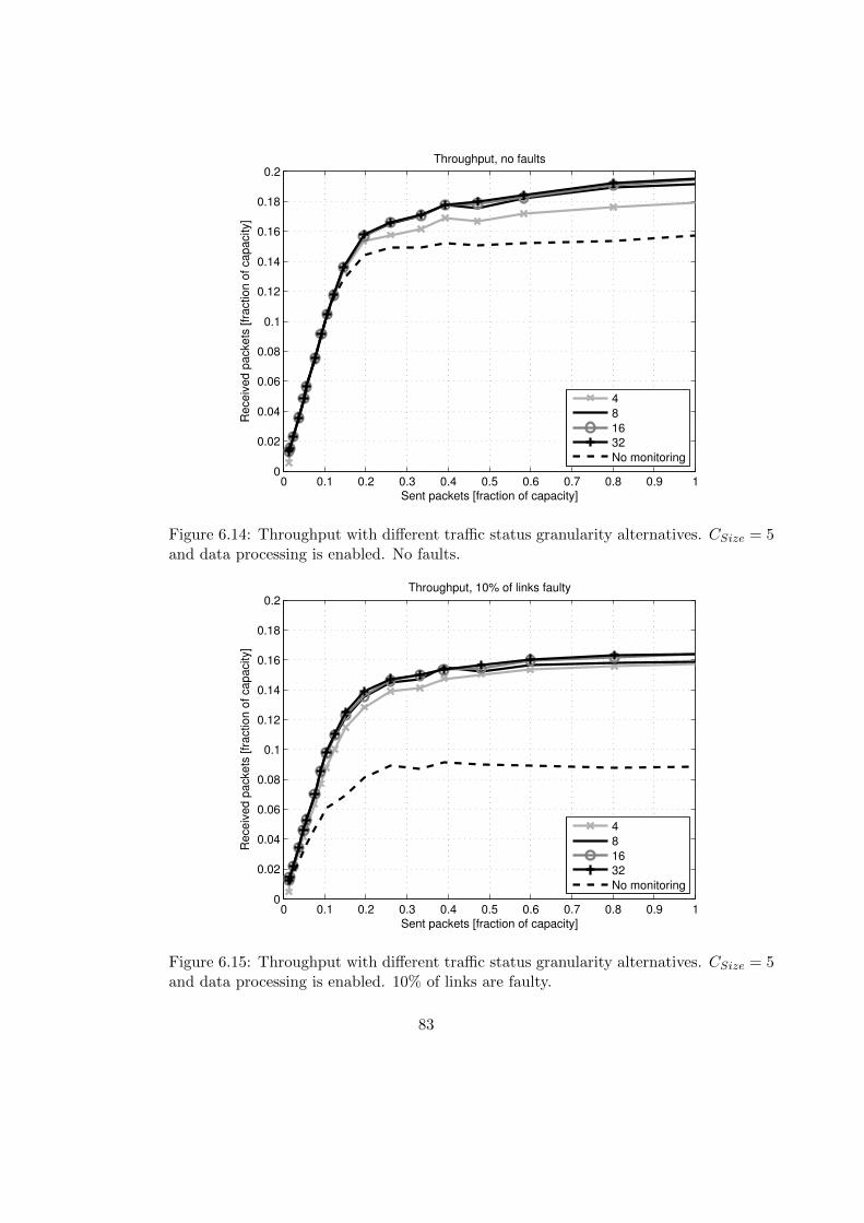
0 0.1 0.2 0.3 0.4 0.5 0.6 0.7 0.8 0.9 10

0.02

0.04

0.06

0.08

0.1

0.12

0.14

0.16

0.18

0.2

Sent packets [fraction of capacity]

Receiv

ed p

ackets

[fr

action o

f capacity]

Throughput, no faults

4

8

16

32

No monitoring

Figure 6.14: Throughput with different traffic status granularity alternatives. CSize = 5and data processing is enabled. No faults.

0 0.1 0.2 0.3 0.4 0.5 0.6 0.7 0.8 0.9 10

0.02

0.04

0.06

0.08

0.1

0.12

0.14

0.16

0.18

0.2

Sent packets [fraction of capacity]

Receiv

ed p

ackets

[fr

action o

f capacity]

Throughput, 10% of links faulty

4

8

16

32

No monitoring

Figure 6.15: Throughput with different traffic status granularity alternatives. CSize = 5and data processing is enabled. 10% of links are faulty.

83

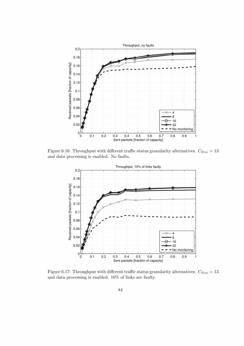
0 0.1 0.2 0.3 0.4 0.5 0.6 0.7 0.8 0.9 10

0.02

0.04

0.06

0.08

0.1

0.12

0.14

0.16

0.18

0.2

Sent packets [fraction of capacity]

Re

ce

ive

d p

acke

ts [

fra

ctio

n o

f ca

pa

city]

Throughput, no faults

4

8

16

32

No monitoring

Figure 6.16: Throughput with different traffic status granularity alternatives. CSize = 13and data processing is enabled. No faults.

0 0.1 0.2 0.3 0.4 0.5 0.6 0.7 0.8 0.9 10

0.02

0.04

0.06

0.08

0.1

0.12

0.14

0.16

0.18

0.2

Sent packets [fraction of capacity]

Re

ce

ive

d p

acke

ts [

fra

ctio

n o

f ca

pa

city]

Throughput, 10% of links faulty

4

8

16

32

No monitoring

Figure 6.17: Throughput with different traffic status granularity alternatives. CSize = 13and data processing is enabled. 10% of links are faulty.

84

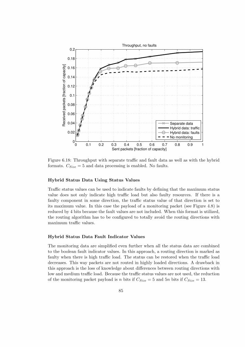
0 0.1 0.2 0.3 0.4 0.5 0.6 0.7 0.8 0.9 10

0.02

0.04

0.06

0.08

0.1

0.12

0.14

0.16

0.18

0.2

Sent packets [fraction of capacity]

Receiv

ed p

ackets

[fr

action o

f capacity]

Throughput, no faults

Separate data

Hybrid data: traffic

Hybrid data: faults

No monitoring

Figure 6.18: Throughput with separate traffic and fault data as well as with the hybridformats. CSize = 5 and data processing is enabled. No faults.

Hybrid Status Data Using Status Values

Traffic status values can be used to indicate faults by defining that the maximum statusvalue does not only indicate high traffic load but also faulty resources. If there is afaulty component in some direction, the traffic status value of that direction is set toits maximum value. In this case the payload of a monitoring packet (see Figure 4.8) isreduced by 4 bits because the fault values are not included. When this format is utilized,the routing algorithm has to be configured to totally avoid the routing directions withmaximum traffic values.

Hybrid Status Data Fault Indicator Values

The monitoring data are simplified even further when all the status data are combinedto the boolean fault indicator values. In this approach, a routing direction is marked asfaulty when there is high traffic load. The status can be restored when the traffic loaddecreases. This way packets are not routed in highly loaded directions. A drawback inthis approach is the loss of knowledge about differences between routing directions withlow and medium traffic load. Because the traffic status values are not used, the reductionof the monitoring packet payload is n bits if CSize = 5 and 5n bits if CSize = 13.

85

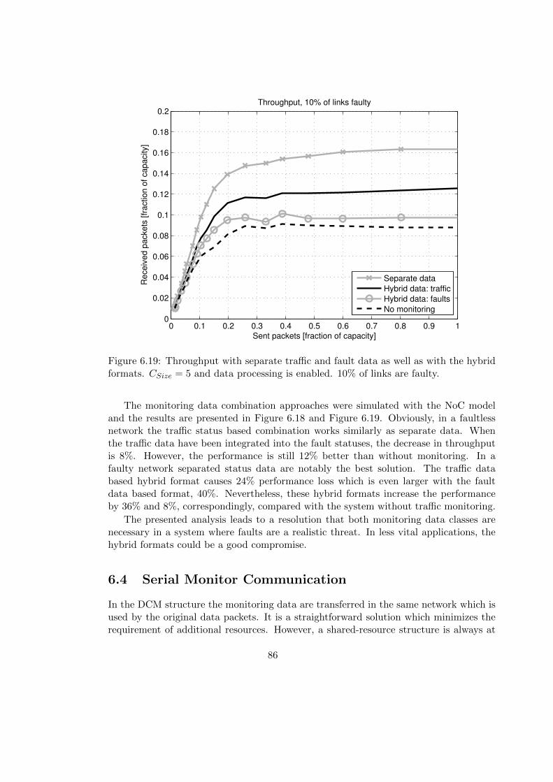
0 0.1 0.2 0.3 0.4 0.5 0.6 0.7 0.8 0.9 10

0.02

0.04

0.06

0.08

0.1

0.12

0.14

0.16

0.18

0.2

Sent packets [fraction of capacity]

Receiv

ed p

ackets

[fr

action o

f capacity]

Throughput, 10% of links faulty

Separate data

Hybrid data: traffic

Hybrid data: faults

No monitoring

Figure 6.19: Throughput with separate traffic and fault data as well as with the hybridformats. CSize = 5 and data processing is enabled. 10% of links are faulty.

The monitoring data combination approaches were simulated with the NoC modeland the results are presented in Figure 6.18 and Figure 6.19. Obviously, in a faultlessnetwork the traffic status based combination works similarly as separate data. Whenthe traffic data have been integrated into the fault statuses, the decrease in throughputis 8%. However, the performance is still 12% better than without monitoring. In afaulty network separated status data are notably the best solution. The traffic databased hybrid format causes 24% performance loss which is even larger with the faultdata based format, 40%. Nevertheless, these hybrid formats increase the performanceby 36% and 8%, correspondingly, compared with the system without traffic monitoring.

The presented analysis leads to a resolution that both monitoring data classes arenecessary in a system where faults are a realistic threat. In less vital applications, thehybrid formats could be a good compromise.

6.4 Serial Monitor Communication

In the DCM structure the monitoring data are transferred in the same network which isused by the original data packets. It is a straightforward solution which minimizes therequirement of additional resources. However, a shared-resource structure is always at

86

0 0.1 0.2 0.3 0.4 0.5 0.6 0.7 0.8 0.9 10

0.02

0.04

0.06

0.08

0.1

0.12

0.14

0.16

0.18

0.2

Sent packets [fraction of capacity]

Receiv

ed p

ackets

[fr

action o

f capacity]

Throughput, 10% of links faulty

4

8

16

32

No monitoring

Monitoring packets

Figure 6.20: Throughput with different granularity alternatives using serial communica-tion. 10% of links are faulty and data processing is enabled. CSize = 5.

least somewhat intrusive and it consumes the network resources which otherwise couldbe used by the actual data packets.

An alternative solution to the inter-monitor communication is serial communicationwhich is implemented with dedicated channels. It can be realized with relatively smallamount of additional resources. A drawback in the serial communication is the increasedtransfer delay. However, because the serial communication resources are dedicated tothe monitoring communication there can be a non-stop status update without payingattention to update intervals. [56]

Serial monitor communication was simulated with the SystemC based NoC simula-tion model. Throughput with different status data granularities and serial communica-tion is presented in Figure 6.20 and Figure 6.21. The serial transmitter operates at thesame clock frequency as the maximum frequency of the monitoring packet transmitter.However, the latter rarely works on its maximum frequency because of the status updateinterval conditions.

Essentially serial communication is slower than the earlier discussed parallel, packetbased communication and the theoretical delays of the serial communication are evenmore increased when there is large amount of data to be transferred for example insystems with relatively large monitoring clusters. However, in contrast the serial com-

87

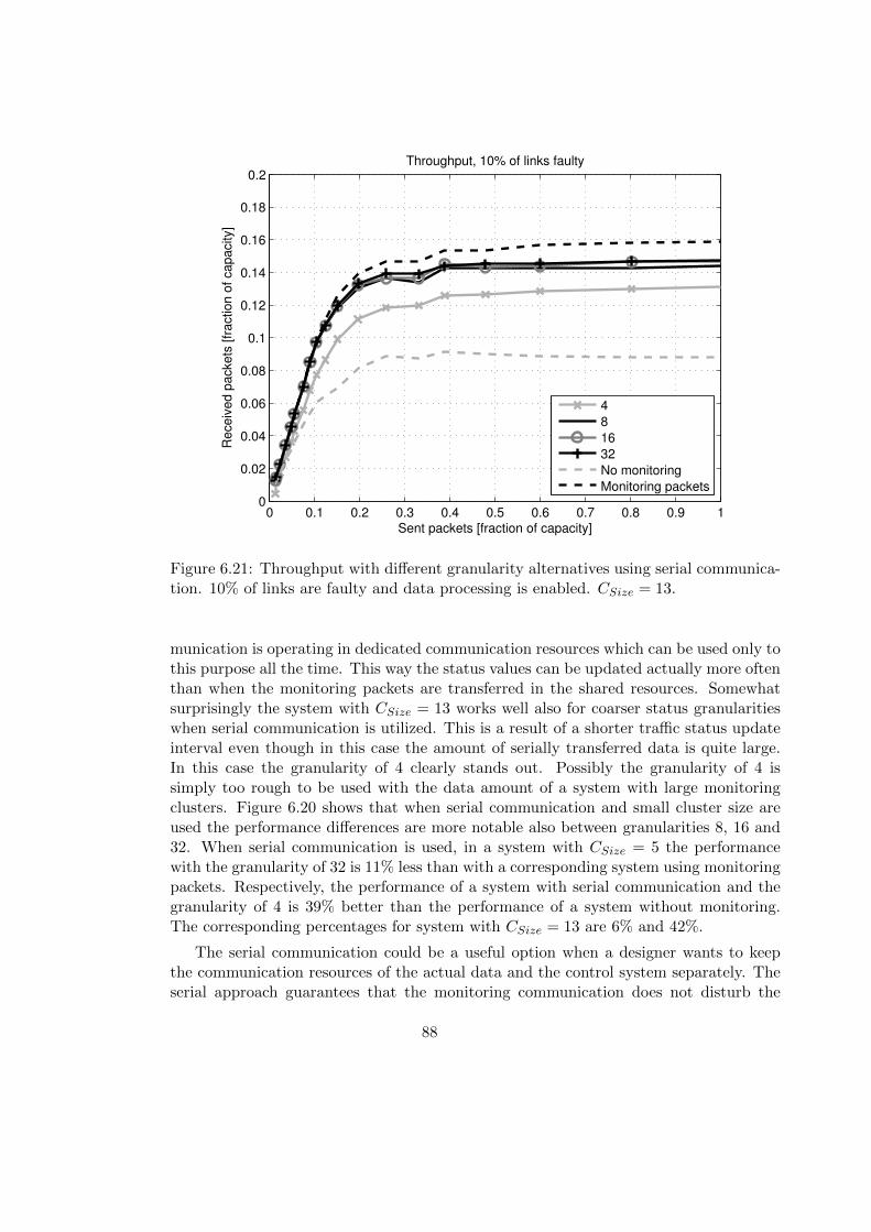
0 0.1 0.2 0.3 0.4 0.5 0.6 0.7 0.8 0.9 10

0.02

0.04

0.06

0.08

0.1

0.12

0.14

0.16

0.18

0.2

Sent packets [fraction of capacity]

Receiv

ed p

ackets

[fr

action o

f capacity]

Throughput, 10% of links faulty

4

8

16

32

No monitoring

Monitoring packets

Figure 6.21: Throughput with different granularity alternatives using serial communica-tion. 10% of links are faulty and data processing is enabled. CSize = 13.

munication is operating in dedicated communication resources which can be used only tothis purpose all the time. This way the status values can be updated actually more oftenthan when the monitoring packets are transferred in the shared resources. Somewhatsurprisingly the system with CSize = 13 works well also for coarser status granularitieswhen serial communication is utilized. This is a result of a shorter traffic status updateinterval even though in this case the amount of serially transferred data is quite large.In this case the granularity of 4 clearly stands out. Possibly the granularity of 4 issimply too rough to be used with the data amount of a system with large monitoringclusters. Figure 6.20 shows that when serial communication and small cluster size areused the performance differences are more notable also between granularities 8, 16 and32. When serial communication is used, in a system with CSize = 5 the performancewith the granularity of 32 is 11% less than with a corresponding system using monitoringpackets. Respectively, the performance of a system with serial communication and thegranularity of 4 is 39% better than the performance of a system without monitoring.The corresponding percentages for system with CSize = 13 are 6% and 42%.

The serial communication could be a useful option when a designer wants to keepthe communication resources of the actual data and the control system separately. Theserial approach guarantees that the monitoring communication does not disturb the

88

actual data which are transferred in the network. It may be possible to increase theclock frequency of the serial transmitter from what was used in the presented analysis.In this case, the performance differences should shrink.

6.5 Reduction of Monitors

The DCM system is based on a structure where there is an identical monitor attachedto each router. These monitors include both monitoring and probing components. Onepotential way to reduce monitoring structure complexity is to decrease the number ofmonitors systematically by removing every nth monitor. In this approach there is aprobe attached to every router but a monitor is attached only to a limited numberof routers. This means that there is still complete knowledge of the network state inthe monitors because there are probes attached to every router. Two monitor removalpatterns are illustrated in Figure 6.22. The monitors receive probed data, process itand deliver it to the local router. The routers, that do not have own monitor, shouldutilize a deterministic routing algorithm because they do not have access to the probedstatus data from the neighboring routers. An adaptive algorithm is utilized in theother routers [14]. The simplified deterministic routers forward packets based on adeterministic routing algorithm. In problematic traffic or fault cases a simplified routercould route packets randomly just directing them to some of its neighbors. In any casethe neighbors of a deterministic router are adaptive routers which can route the packetforward adaptively.

In addition to performance, the reduction of monitors affects the complexity of theNoC implementation. Routers which do not have own monitoring component couldhave less complex routing logic which decreases the router area. This is due to thedeterministic routing algorithm which substitutes the adaptive routing algorithm in the

X X

X X X

X X X

X X

X X X

X

X

X

X

X

X

X

XEvery 3rd monitor removed.

X

X

X

X

X

X

X

X

X

XEvery 6th monitor removed.

Figure 6.22: Two patterns of removed monitors. Removed monitors are marked with X.

89

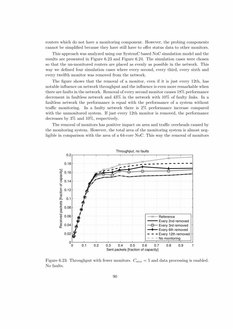
routers which do not have a monitoring component. However, the probing componentscannot be simplified because they have still have to offer status data to other monitors.

This approach was analyzed using our SystemC based NoC simulation model and theresults are presented in Figure 6.23 and Figure 6.24. The simulation cases were chosenso that the un-monitored routers are placed as evenly as possible in the network. Thisway we defined four simulation cases where every second, every third, every sixth andevery twelfth monitor was removed from the network.

The figure shows that the removal of a monitor, even if it is just every 12th, hasnotable influence on network throughput and the influence is even more remarkable whenthere are faults in the network. Removal of every second monitor causes 18% performancedecrement in faultless network and 43% in the network with 10% of faulty links. In afaultless network the performance is equal with the performance of a system withouttraffic monitoring. In a faulty network there is 2% performance increase comparedwith the unmonitored system. If just every 12th monitor is removed, the performancedecreases by 3% and 10%, respectively.

The removal of monitors has positive impact on area and traffic overheads caused bythe monitoring system. However, the total area of the monitoring system is almost neg-ligible in comparison with the area of a 64-core NoC. This way the removal of monitors

0 0.1 0.2 0.3 0.4 0.5 0.6 0.7 0.8 0.9 10

0.02

0.04

0.06

0.08

0.1

0.12

0.14

0.16

0.18

0.2

Sent packets [fraction of capacity]

Receiv

ed p

ackets

[fr

action o

f capacity]

Throughput, no faults

Reference

Every 2nd removed

Every 3rd removed

Every 6th removed

Every 12th removed

No monitoring

Figure 6.23: Throughput with fewer monitors. Csize = 5 and data processing is enabled.No faults.

90

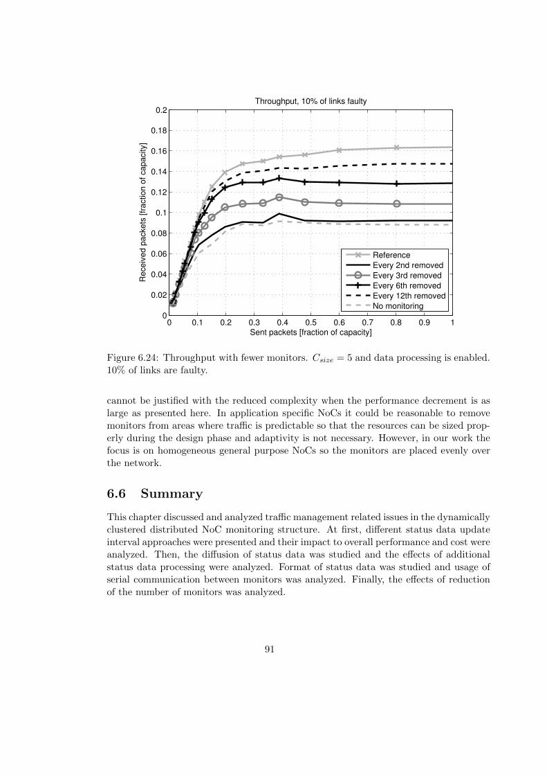
0 0.1 0.2 0.3 0.4 0.5 0.6 0.7 0.8 0.9 10

0.02

0.04

0.06

0.08

0.1

0.12

0.14

0.16

0.18

0.2

Sent packets [fraction of capacity]

Receiv

ed p

ackets

[fr

action o

f capacity]

Throughput, 10% of links faulty

Reference

Every 2nd removed

Every 3rd removed

Every 6th removed

Every 12th removed

No monitoring

Figure 6.24: Throughput with fewer monitors. Csize = 5 and data processing is enabled.10% of links are faulty.

cannot be justified with the reduced complexity when the performance decrement is aslarge as presented here. In application specific NoCs it could be reasonable to removemonitors from areas where traffic is predictable so that the resources can be sized prop-erly during the design phase and adaptivity is not necessary. However, in our work thefocus is on homogeneous general purpose NoCs so the monitors are placed evenly overthe network.

6.6 Summary

This chapter discussed and analyzed traffic management related issues in the dynamicallyclustered distributed NoC monitoring structure. At first, different status data updateinterval approaches were presented and their impact to overall performance and cost wereanalyzed. Then, the diffusion of status data was studied and the effects of additionalstatus data processing were analyzed. Format of status data was studied and usage ofserial communication between monitors was analyzed. Finally, the effects of reductionof the number of monitors was analyzed.

91

92

Chapter 7

Lightweight Task Mapping

Task mapping is an essential part of management of a multiprocessorNetwork-on-Chip. In conventional processor systems tasks can be assigned staticallyto processor cores during the design phase of the system. However, when there are tensor hundreds of cores static mapping cannot exploit the full potential of the NoC in termsof flexibility, scalability and performance. A large NoC is able to accommodate a lot ofdifferent kind of tasks in various sizes. This capability is strongly limited if mapping hasto be carried out once and it cannot be reconfigured run time. An obvious solution tothis is dynamic task mapping which customizes task mapping during operation of thesystem. The goal of task mapping is to find the trade-off between maximal processorutilization and minimum communication resource utilization [74].

The task mapping methods can be roughly categorized in terms of three factors. Thefirst factor is the used system metrics that affect the mapping decisions. These metricsare basically computational load of cores and traffic load of the network. The loadmetrics show how much there are free computational and communication resources thatcan be assigned for new tasks. These metrics can be used individually or in conjunction.The second factor is the type of mapping implementation which can be centralized ordistributed. In the centralized approach there is a mapping processor which has completeoverall knowledge of the status of the system and makes all the mapping decisions. Ina distributed approach the mapping process is distributed in several units around thesystem and it is carried out without centralized control. Finally, the third categorizationfactor is the type of the mapping itself. The mapping can be static or dynamic. Staticmapping is done once and it remains unchanged during the operation of the system.Dynamic mapping has a starting point when the tasks are mapped during the systeminitialization, but the mapping can change and new tasks may be mapped during runtime.

Centralized mapping shares the same strengths and weaknesses as any centralizedsystem. They are relatively easy to implement and control because all the information iscollected into one place in the system. It is also good in terms of area overhead becauseonly one mapping processor is required. On the other hand, a centralized mapping is

93

fragile for faults and causes high monitoring and mapping traffic load especially aroundthe central controller.

Some characteristics, used in distributed run-time task mapping, are previously pre-sented in different research articles. A run-time agent-based distributed applicationmapping for on-chip communication has been presented in [4]. It is designed for hetero-geneous multiprocessor systems. The approach presented in [4] uses fixed virtual clustersand cluster agents which take care of task mapping in a cluster. There are also globalagents which map applications to different clusters.

Communication-aware heuristics for run-time task mapping on NoC-based MPSoC(multiprocessor System-on-Chip) has been presented in [61]. Four run-time mappingheuristics have been presented including mapping strategies which map a new task forexample to their nearest neighbor systematically or by choosing the best neighbor avail-able. The mapping can be also communication-aware in a way that the distance betweentwo communicating tasks is tried to be minimized.

A decentralized task mapping approach for homogeneous multiprocessor NoCs hasbeen presented in [74]. The mapping is based on local information on processor workload,task size, communication requirements and link contention. This information is collectedonly from a close vicinity of a core. The presented task mapping algorithm tries to findbetter mapping for current task scheme in the system.

Our goal is to extend the previously presented dynamically clustered network mon-itoring structure to be used as a part of a lightweight task mapping mechanism. Thecores of the system should be able to independently assign tasks to other cores. Theproposed task mapping mechanism is based on the idea of mapping tasks to the bestavailable neighbor core. The idea behind our solution is that a core initiates task map-ping by sending a mapping packet to another core which seems to be the best from itsown point of view. Mapping packets are discussed in Section 7.2. Finally, the task endsup mapped to a core. The task can be mapped to a core where the initiator core sent themapping packet at the beginning or the task can be remapped further to a less loadedcore. The initiator core is only interested about the fact that the task will be executedproperly with a reasonable performance, without regarding which core does it.

7.1 Lightweight Distributed Task Mapping

Our lightweight distributed task mapping is based on the dynamically clustered monitor-ing (DCM) structure (see Chapter 4). The DCM structure [55, 58] is originally designedfor traffic management purposes to collect traffic status and fault data from a network.In this chapter the monitoring structure is enhanced and applied for dynamic run-timetask mapping purposes.

The task mapping mechanism is designed to be as lightweight as possible so thatacceptable performance can be reached with minimal area overhead. Intrusiveness ofrun-time task mapping is also taken into account because any run-time managementoperation should not interfere with the main operations of the system. The lightweight

94

task mapping is distributed to the monitors all around the network, which makes itflexible and highly scalable. As the system is distributed, the added energy consumptionand heat generation are also distributed over the whole system. The communicationoverhead is also moderate due to the lack of centralized control and long-distance controlrelated communication. Task mapping functionality is allocated into monitors and coresso that the monitors take care of the neighbor core evaluation and the cores make themapping decisions. The system does not try to pursue optimal task mapping schemes butgood mapping schemes which lead to acceptable overall performance while maintainingthe other goals including flexibility, scalability and low intrusiveness.

Monitoring and mapping processes are distributed to cores and to separate monitor-ing components which are directly connected to the cores. The monitors collect networkand computational load information from their neighborhood and offer this data, com-bined with their own statuses, to their own neighbors. This way the cores do not onlyhave knowledge of their neighbors’ statuses but also wider overall knowledge of net-work and computational load in different directions in the network. The neighbor datacollection and the monitoring principles were presented in Chapter 3.

Typically, tasks are mapped to the processors in the initialization phase of the systemand the execution of these initial tasks begins. This initial mapping can be done staticallyduring the design phase of the system or it can be left to the responsibility of an operatingsystem. The idea of the dynamic run-time task mapping is that while the initial taskmapping has been carried out at the initialization phase, the computational cores areable to map new tasks at run-time independently without centralized control. This waythe operation of the system is flexible and the run-time reconfiguration does not causesignificant load to the system.

The status data in the distributed monitoring are collected from the neighbors andthe received data can also include data from the neighbors’ neighbors. Therefore, amonitor does not have complete knowledge of the network but only the status of thecores and routers in its own dynamic cluster (see Chapter 4). Complete knowledge isnot essential because one of the main principles of the lightweight task mapping is tominimize the distance between tasks which are communicating with each other. Lowercomputing performance could be beneficial if higher computing performance causes alot of long-distance communication, because overall performance is the joint effect ofcomputational and communication performance. Mapping to a remote core on the otherside of the network is possible if necessary. This has been made possible by a taskremapping mechanism which can forward a mapping packet until a suitable core hasbeen found. The remapping is discussed later in this chapter.

One essential principle in the lightweight task mapping mechanism is that the initialmapper does not know in the beginning where its task will finally be mapped. Thisknowledge is irrelevant. All that a core has to know is that the task will end up to acore where it can be executed with acceptable performance. When the task has beenmapped, the original mapper is informed where the task resides. This information is notneeded prior to completion of the mapping.

95

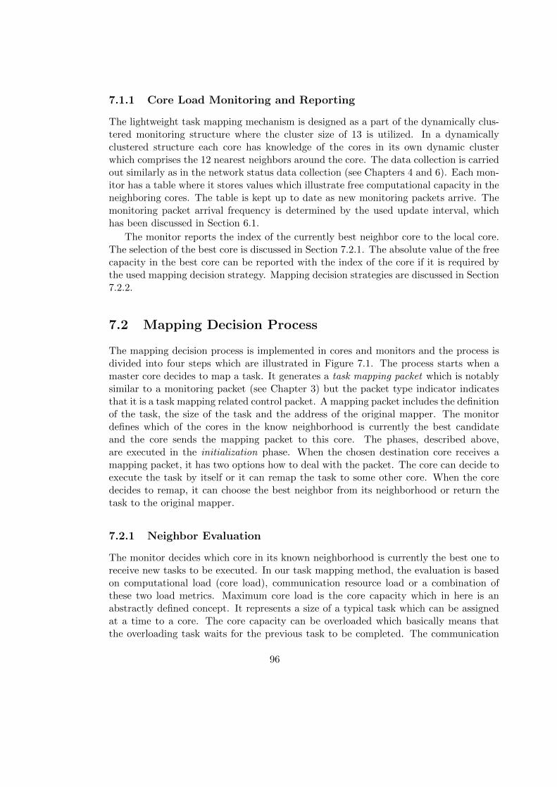
7.1.1 Core Load Monitoring and Reporting

The lightweight task mapping mechanism is designed as a part of the dynamically clus-tered monitoring structure where the cluster size of 13 is utilized. In a dynamicallyclustered structure each core has knowledge of the cores in its own dynamic clusterwhich comprises the 12 nearest neighbors around the core. The data collection is carriedout similarly as in the network status data collection (see Chapters 4 and 6). Each mon-itor has a table where it stores values which illustrate free computational capacity in theneighboring cores. The table is kept up to date as new monitoring packets arrive. Themonitoring packet arrival frequency is determined by the used update interval, whichhas been discussed in Section 6.1.

The monitor reports the index of the currently best neighbor core to the local core.The selection of the best core is discussed in Section 7.2.1. The absolute value of the freecapacity in the best core can be reported with the index of the core if it is required bythe used mapping decision strategy. Mapping decision strategies are discussed in Section7.2.2.

7.2 Mapping Decision Process

The mapping decision process is implemented in cores and monitors and the process isdivided into four steps which are illustrated in Figure 7.1. The process starts when amaster core decides to map a task. It generates a task mapping packet which is notablysimilar to a monitoring packet (see Chapter 3) but the packet type indicator indicatesthat it is a task mapping related control packet. A mapping packet includes the definitionof the task, the size of the task and the address of the original mapper. The monitordefines which of the cores in the know neighborhood is currently the best candidateand the core sends the mapping packet to this core. The phases, described above,are executed in the initialization phase. When the chosen destination core receives amapping packet, it has two options how to deal with the packet. The core can decide toexecute the task by itself or it can remap the task to some other core. When the coredecides to remap, it can choose the best neighbor from its neighborhood or return thetask to the original mapper.

7.2.1 Neighbor Evaluation

The monitor decides which core in its known neighborhood is currently the best one toreceive new tasks to be executed. In our task mapping method, the evaluation is basedon computational load (core load), communication resource load or a combination ofthese two load metrics. Maximum core load is the core capacity which in here is anabstractly defined concept. It represents a size of a typical task which can be assignedat a time to a core. The core capacity can be overloaded which basically means thatthe overloading task waits for the previous task to be completed. The communication

96

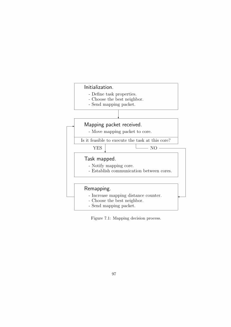
- Choose the best neighbor.- Send mapping packet.

- Define task properties.

- Notify mapping core.- Establish communication between cores.

- Increase mapping distance counter.- Choose the best neighbor.- Send mapping packet.

?

-

?

�

NOYES

Initialization.

Mapping packet received.- Move mapping packet to core.

Is it feasible to execute the task at this core?

Task mapped.

Remapping.

Figure 7.1: Mapping decision process.

97

resource load is the same metric which is used in traffic management to reconfigureadaptive routing at run-time (see Chapter 6).

Core-Load-Aware Evaluation

Core-load-aware neighbor evaluation is the simplest evaluation option. The monitorcompares the core load values of its neighbors and chooses the one with the highest freecapacity as the currently best neighbor core. The core load values are defined so that acore measures its current load (Cused) and subtracts it from its maximum computationalcapacity (Cmax). This result is the current free capacity (Cfree) of the core and it isused as a core status value in the core-load-aware evaluation.

Cfree = Cmax − Cused (7.1)

Communication-Aware Evaluation

Communication in the network is mainly caused by the tasks which communicate witheach other. If we define that memory accesses and I/O communication are also essen-tially tasks, all communication takes place between tasks. Therefore, there should bea relation between the computational core load and communication resource load. Asimple communication-aware neighbor evaluation uses only the traffic monitoring dataand chooses the best neighbor core based on this traffic information. The traffic status(Straffic) is calculated using Equation 6.3 (see Section 6.2.1). This is a very lightweightmapping solution because there is no need for the core load monitoring at all. However,one can assume that the accuracy suffers when the decisions are based on secondaryinformation, the communication load information in this case.

Core-Load- and Communication-Aware Evaluation

The third neighbor evaluation approach is a combination of the above evaluation ap-proaches. It is both core-load- and communication-aware. The core load and commu-nication statuses are combined to a single status value which represents both the freecomputational capacity and the status of the communication resources. The core loadstatus values show the amount of free capacity so that a larger value represents smallercore load and that way a larger amount of free capacity. The traffic status values, whichare used to measure the load of communication resources, represent the traffic status sothat a larger value corresponds to a larger load in the network. A combined core loadand communication status value (Ccombined) is calculated using equation

Ccombined = Cfree − Straffic, (7.2)

where Cfree is calculated using Equation 7.1 and Straffic is the traffic status value inthe direction of the core. Finally, the selection of the best neighbor core is based on theranking of these combined core load and communication values. An additional weight

98

factor can be utilized to adjust the significance of the traffic status in Equation 7.2. In thepresented communication-aware evaluation approaches the available fault information isutilized so that tasks are not mapped in directions where a fault has been observed.

7.2.2 Mapping Decision Strategies

The task mapping decision strategy defines what a core does when it receives a taskmapping packet. There are three procedures to select from: the core can take over thetask and the mapping is completed, the core can do a remapping and map the taskforward to a core which seems the best from its point of view, or the core can return themapping packet to the original mapper. This study includes four different task mappingdecision strategies which execute these three procedures based on the defined strategy.These strategies are presented below.

1. Remapping forward if there is not enough free capacity for the task in the currentcore. The task is remapped as long as it ends up to a suitable core. The disad-vantage of this decision strategy is that the mapping distance is unbounded. Thetasks can be mapped far away from the mapper and if there is no suitable core inthe network, the mapping packet is finally dropped similarly as un-routable datapackets. If the mapping packet is dropped the task will not be completed and theorginator of the task has to initiate another instance of the same task mapping.

2. Core capacity overloading if mapping distance exceeds a statically defined distancethreshold even if there is not enough free capacity in the current core. There isa counter in a mapping packet which shows how many times the mapping hasbeen tried. Naturally this has a negative impact on the system performance. Thisdecision strategy eliminates the disadvantage of the mapping strategy 1. However,the core overloading has a negative influence to the system performance. Themapping distance is bounded with the distance threshold and thus it can be keptmoderate.

3. Capacity overloading if there is not enough free capacity in the known neighbor-hood. This strategy requires knowledge of the amount of free capacity in theneighboring cores so that the monitor has to report not only the ID of the bestneighbor but also the amount of its free capacity. Performance-wise this is a goodstrategy because when a core is overloaded the distance between the mapper coreand the mapped tasks remains moderate. The mapping distances can be kepteven shorter than in decision strategy 2. However, this strategy requires highermonitoring complexity due to detailed capacity reporting.

4. Remapping backwards if not enough free capacity in the known neighborhood orin the current core. This strategy is similar to the previous (3) strategy. Thedifference is that when enough free capacity cannot be found, the current coreis not overloaded but the mapping packet is returned to the mapper. In this

99

case the original mapper core recognizes that the packet is returned and overloadsitself. In terms of performance there is a compromise that when core overloadingis required the communication between cores is eliminated. The elimination ofinter-core communication increases performance by lowering the communicationresource load. However, packet returning and identification of returned mappingpackets requires even more complex logic than the decision strategy 3.

7.3 Enhanced Monitoring System

Several modifications to the monitoring system are made to enable the task mapping inthe dynamically clustered Network-on-Chip. The main improvements concern core andmonitor modules while there are also smaller modifications in the router attributes andpacket structure.

Each core has two new parameters, capacity and load. Capacity represents the com-putational capability of a core while load indicates how many units of the capacity iscurrently used. Capacity in this framework is an abstract concept (see Section 7.2.1).It can be seen as a typical maximum size of the task queue in a core. However, there isa possibility to overload a core by extending the size of the task queue. The core alsohas mechanisms to initiate task mapping, to assign a task to itself and to remap a taskfurther.

Monitor components have been developed further to be able to collect also the coreload data in addition to the network status information. An enhanced monitor alsoincludes neighbor evaluation mechanisms which rank the neighbors and chooses thecurrently best neighbor core based on the used evaluation approach.

The routers are modified so that the task mapping packets have the second highestpriority after monitoring packets. The prioritization is required to prevent mappingpackets to get stuck in the network. However, the priority is not seen as important asthe priority of the monitoring packets because in a highly loaded network the mappingof new tasks is arguable. The implementation of task mapping features in the simulationenvironment has been discussed in Section 5.4.5.

7.4 Case Study: Mapping Tasks

The functionality of the lightweight distributed task mapping algorithm was demon-strated as a case study. The demonstration was carried out using the presented NoCsimulation environment (see Chapter 5). A mesh-shaped NoC containing 64 cores androuters (8 x 8) was modeled. The details to be examined concern the number of mappingdecision attempts, distances between the mappers and the mapped tasks as well as theamount of failed mappings. The distribution of the computational core load was alsoexamined. The used neighbor evaluation approaches are denoted as in Table 7.1. Thenotation of mapping decision strategies was presented in Section 7.2.

100

Table 7.1: Neighbor evaluation approaches.

Description

a Core load based evaluation.

b Communication based evaluation.

c Combined core load and communication based evaluation.

The purpose of this demonstration is not to find an absolute answer to which ofthese presented mapping strategies and evaluation approaches are the best in any givenapplication. The case study is based on comparison of the mapping approaches and itis realized using examples showing how their functionality differs in a specific situation.The demonstration scheme has been chosen so that it would show the essential propertiesof different mapping approaches when the system is loaded with new tasks. The mappercores are located in a large area in the middle of the network so that balanced taskmapping is possible. To imitate mapping schemes of real systems the mapper area isnot symmetric.

The starting point for the simulations is a 64-core NoC without any traffic or com-putational load on any core. During the simulation 14 cores initiate a task mappingone after another. These 14 cores are shown in Figure 7.2. This is repeated 4 times sothat each of these cores initiates and sends 4 mapping packets totalling 56 tasks to bemapped. The example system consists of identical multipurposes cores so that each task

Figure 7.2: Task mapping initiator cores marked with gray.

101

Table 7.2: Task mapping results.

MDS NEA Task distance Mapping decisions Drop-%

1 a 1.74 1.23 16.071 b 2.00 2.10 64.291 c 1.87 1,38 16.07

2 a 1.91 1.42 0.002 b 1.91 2.11 0.002 c 1.98 1.43 0.00

3 a 1.71 1.13 0.003 b 1.09 1.07 0.003 c 1.79 1.18 0.00

4 a 1.48 1.23 0.004 b 0.32 1.75 0.004 c 1.34 1.25 0.00

MDS: Mapping

decision strategy.NEA: Neighbor evaluation approach.

Task distances and mapping decisions are average values.

can be executed in any of the cores. Communication in the network is modelled so thatthere is continuous communication between a mapper and the related core in which thetask is mapped.

The results of the case study demonstration are collected into Table 7.2. Notice,that when using the decision strategy 1 the mapping packet drop percentage is verylarge especially when the communication-aware neighbor evaluation is used (64,29 %).High drop rate indicates that simple communication-aware neighbor evaluation does notreflect the computational status well enough. Because of the core overload mechanismof the other decision strategies, the mapping packet drop does not exist when thosestrategies are used.

The differences in the task distances and mapping decision attempt counts are notthat prominent. The minimum of the task distances is reached using the decision strategy4. The short task distances are explained by the mapping returning mechanism whicheliminates the communication completely in some of the cases.

The computational core load at the end of each simulation is illustrated in Figure7.3, Figure 7.4, Figure 7.5 and Figure 7.6. The color of the core shows the amount of theload. White cores are not loaded at all while black cores are highly overloaded. As can benoticed the purely communication-aware evaluation approach causes significantly unevencore load distribution. As was mentioned previously, there is a correlation betweencore load and communication resource load even though the relation is not perfect.An obvious uncertainty is caused by the fact that communication between two coresdistributes the communication load evenly on the network path between these cores.

102

Core capacity Communication capacity Combined

Figure 7.3: Core load with mapping decision strategy 1.

Core capacity Communication capacity Combined

Figure 7.4: Core load with mapping decision strategy 2.

Core capacity Communication capacity Combined

Figure 7.5: Core load with mapping decision strategy 3.

Core capacity Communication capacity Combined

Figure 7.6: Core load with mapping decision strategy 4.

103

External observer cannot separate routers which are connected to a highly loaded corefrom routers which are just situated along a highly loaded network path. Network statusdata are also partly inaccurate because it shows the load of a router and not the exactload of a link. This inaccuracy has been discussed in Chapter 3.

Other evaluation approaches lead to moderately even load distribution. One can notethat when decision strategy 4 is applied the number of overloaded cores is somewhathigher than with the other strategies. These overloaded cores are mostly situated in themiddle of the network and middle of the area of mapper cores (see Figure 7.2). Thetasks which are initialized from the middle of the loaded area end up more probablyin situation where the task cannot be mapped. In this kind of situation the strategy 4returns the mapping packet to the mapper core. This causes concentrated overloadingin the middle of the highly loaded area.

While the strategy 1 causes unacceptable mapping packet dropping it seems thatthe decision strategies 2 and 3 with core-load-aware or combined neighbor evaluationapproach (a or c) are the considerable alternatives. In this case study, the usage ofcommunication status information in the combined neighbor evaluation approach doesnot cause notable load distribution differences in one direction or another. However, theoverhead of combined evaluation related to the core-load-aware evaluation is minimalbecause the communication status information is anyway available in monitors.

7.5 Summary and Future Work

A task mapping approach applying the previously presented DCM structure was pre-sented and its functionality demonstrated in this chapter. The presented demonstrationshows that an enhanced DCM structure is suitable for lightweight task mapping pur-poses. Lightweight task mapping does not aim for perfect mapping results but schemeswith acceptable performance so that run-time task mapping is enabled. The mechanismis lightweight so that reasonable mapping performance can be reached with minimalcomplexity, energy and area overhead. Four different mapping decision processes andthree neighbor evaluation approaches were studied. The demonstration shows that coreload monitoring is essential in task mapping and it cannot be fully replaced with com-munication monitoring even though core load and communication load are related toeach other.

The core load monitoring protocol steers tasks to the best cores in the known neigh-borhood. The goal is to make the process as simple and lightweight as possible. Theoptimal solution would choose not the best but the most suitable core, taking into ac-count that it is not always profitable to accommodate small tasks to the cores with thelargest free capacity. Then, for instance, small task would be mapped on a core whichhas free capacity just for a small task and it cannot accommodate larger tasks. However,if the task sizes are equalized the difference between lightweight and optimal solutionsdecreases.

In this chapter the basic functionality of the presented task mapping algorithm was

104

demonstrated in a form of a case study. In future works a more comprehensive analysisshould be carried out to generalize the results and adjust the features of the presentedalgorithm.

105

106

Chapter 8

Conclusions

Dynamic monitoring methods for Networks-on-Chip were studied and a dynamicallyclustered distributed monitoring approach was presented and analyzed in this thesis. Es-sential background information concerning principles of Networks-on-Chip were studiedincluding different topologies, routing algorithms, network flow control as well as com-mon problems on NoCs. Monitoring of Networks-on-Chip was discussed and differentmonitoring structures were studied. Finally, issues concerning the presented dynamicallyclustered monitoring structure (DCM) were discussed and analyzed using an in-housesimulation environment.

Our analysis shows that centralized monitoring is slow and causes significant com-munication overhead to the system while there are tasks, especially related to trafficmanagement, which can be implemented without centralized control. A selection be-tween dedicated and shared resources is an essential decision in terms of intrusiveness,performance and area overhead of a monitoring system. If the designer decides to usededicated resources, it could be reasonable to use centralized monitoring. Otherwise,if shared resources are used, at least network management should be distributed tominimize the need for centralized control and the complexity of centralized monitors.In a large, complex system it may also be reasonable to use hybrid monitoring struc-tures. A hybrid monitoring structure has both distributed and centralized monitoringservices, possibly also clustered services, in the same system. Relatively simple and fre-quently repeated network monitoring tasks are carried out using distributed monitoringwhich optimizes the network resource utilization. The centralized monitoring is typicallyneeded for system diagnostic purposes and for tasks which cannot be executed withoutcentralized control. Traffic management is basically quite regional which means thatmost of the traffic related problems can be solved using the resources near the prob-lematic areas. In most of the cases there is no need to know the situation at the otherside of the network but the status of the neighbors, their neighbors and so on as far asrequired. This decreases the need for centralized control and releases resources for othertasks, for instance load balancing, optimization and reconfiguration.

The work, presented in this thesis, includes extensive analysis of the dynamically

107

clustered distributed monitoring approach. To make the analysis possible an in-houseSystemC based NoC simulation environment was designed and implemented. It hasbeen proved to be an efficient tool for analyzing and simulating different aspects inNetworks-on-Chip. The simulation environment can be easily configured for analysis ofdifferent features which makes it a flexible tool for early phase analysis. The simulationenvironment was used to analyze monitoring algorithms, monitoring data diffusion areas,the format of monitoring data and communication as well as the number of monitors.The presented research shows that in most cases simple monitoring algorithms and smallmonitoring cluster areas perform at least as well as more complex implementations. Inthis thesis the added value of more complex monitoring structures was found small ornegligible in terms of performance. Thus, acceptable monitoring performance can bereached using relatively simple monitoring structures. Another observation is that evensmall adjustments in the system parameters, such as monitoring data update frequenciesor numbers of used monitors, can have a significant influence to the overall performance.Therefore the parameters should be chosen carefully while designing complex distributedmonitoring structures.

The presented DCM structure was applied for task management to analyze its flexibil-ity for purposes other than traffic management. The presented distributed task mappingmethod was analyzed with the NoC simulation environment using different mapping deci-sion strategies and various neighbor evaluation approaches. The analysis showed that thedynamically clustered monitoring structure can be utilized for autonomous distributedtask mapping. It was also noted that proper functionality of the distributed task map-ping requires accurate information about computational load of cores. Even though thecommunication resource load is related to computational load, it is not accurate enoughto be applied for task mapping purpose.

The proposed distributed monitoring system is flexible and scalable, which makes issuitable for Networks-on-Chip because flexibility and scalability are natural characteris-tics of these on-chip networks. Distributing the functionality and partitioning the systeminto smaller parts improves system level fault tolerance because then a faulty componentcannot have severe influence on the overall functionality of the system. The presentedanalysis shows that distributed monitoring systems load the network less than typicalcentralized systems. Fault tolerance, communication overhead and diffusion of monitor-ing data can be improved by clustering a system into smaller parts. However, clusteredstructures do not reach the performance of totally distributed monitoring systems. Themain drawback of distributed monitoring is the lack of global status information whichmay be required in reconfiguration tasks such as system-level energy consumption opti-mization. The outcome is that in large and complex systems it can be beneficial to haveboth centralized and distributed structures.

Performance of the DCM structure could be adjusted by using different sized mon-itoring clusters in different areas in the network. Areas with low traffic load may workat reasonable performance using very simple deterministic routing algorithms. At thesame time in the same system, there could be performance critical areas with hightraffic loads and strict quality of service requirements. Larger monitoring clusters and

108

adaptive routing algorithms are suitable for these critical areas. The cluster sizes androuting algorithms can be made run time reconfigurable to enable extensive optimizationcapability.

In design of complex multiprocessor systems, the focus should be kept on the compu-tational features while the implementation of the communication infrastructure shouldbe straightforward without time consuming design of essential structures. Reusable andfully scalable distributed monitoring structures can be utilized in systems of differentsizes without complicated customization processes. The structures should be developedtowards general communication platforms which conform to different systems with vary-ing performance and operational requirements.

The work presented in this thesis has notable potential for further development. Thepresented NoC simulation environment can be extended and developed for analysis ofdistinct new systems and features. The foundations of dynamically clustered networkmonitoring have been presented and analyzed in this thesis. Future work should leadthe DCM structure towards physical implementations as parts of high performance mul-tiprocessor systems.

109

110

Bibliography

[1] SystemC. http://www.accellera.org/.

[2] M.A. Al Faruque, T. Ebi, and J. Henkel. ROAdNoC: Runtime observability for anadaptive Network on Chip architecture. In IEEE/ACM International Conferenceon Computer-Aided Design, ICCAD 2008, pages 543–548, November 2008.

[3] M.A. Al Faruque, T. Ebi, and J. Henkel. AdNoC: Runtime adaptive network-on-chip architecture. IEEE Transactions on Very Large Scale Integration (VLSI)Systems, 20(2):257–269, February 2012.

[4] M.A. Al Faruque, R. Krist, and J. Henkel. Adam: Run-time agent-based distributedapplication mapping for on-chip communication. In 45th ACM/IEEE Design Au-tomation Conference, DAC 2008, pages 760–765, June 2008.

[5] M. Ali, M. Welzl, and S. Hellebrand. A dynamic routing mechanism for networkon chip. In 23rd NORCHIP Conference, pages 70–73, November 2005.

[6] S. Amstutz. A new store and forward message switching system. IEEE Transactionson Communication Technology, 19(4):528 –529, August 1971.

[7] D. Andreasson and S. Kumar. Slack-time aware routing in noc systems. In IEEEInternational Symposium on Circuits and Systems, pages 2353–2356, May 2005.

[8] N. Bansal, A. Blum, S. Chawla, and A. Meyerson. Online oblivious routing. InProceedings of the fifteenth annual ACM symposium on Parallel algorithms andarchitectures, pages 44–49, 2003.

[9] L. Benini and G. De Micheli. Networks on Chip: a new paradigm for Systems onChip design. In Design, Automation & Test in Europe, DATE ’02, pages 418–419,2002.

[10] D. Bertozzi, L. Benini, and G. De Micheli. Error control schemes for on-chip com-munication links: the energy-reliability tradeoff. IEEE Transactions on Computer-Aided Design of Integrated Circuits and Systems, 24(6):818–831, June 2005.

111

[11] A. Borella, G. Cancellieri, F. Chiaraluce, and F. Meschini. Tree topologies in atmnetworks. In Singapore ICCS/ISITA ’92. ’Communications on the Move’, volume 1,pages 162–166, November 1992.

[12] C. Ciordas, T. Basten, A. Radulescu, K. Goossens, and J. Van Meerbergen. Anevent-based monitoring service for Networks on Chip. ACM Transactions on DesignAutomation of Electronic Systems, 10(4):702–723, 2005.

[13] C. Ciordas, K. Goossens, A. Radulescu, and T. Basten. NoC monitoring: impacton the design flow. In IEEE International Symposium on Circuits and Systems,ISCAS 2006, pages 1981–1984, 2006.

[14] W. J. Dally and B. Towles. Principles and Practices of Interconnection Networks.Morgan Kaufmann, 2004.

[15] W.J. Dally. Virtual-channel flow control. IEEE Transactions on Parallel and Dis-tributed Systems, 3(2):194 –205, March 1992.

[16] W.J. Dally and B. Towles. Route packets, not wires: On-chip interconnectionnetworks. In Design Automation Conference, pages 684–689, 2001.

[17] M. Dehyadgari, M. Nickray, A. Afzali-kusha, and Z. Navabi. Evaluation of pseudoadaptive xy routing using an object oriented model for noc. In The 17th Interna-tional Conference on Microelectronics, December 2005.

[18] J. Duato, S. Yalamanchili, and L. Ni. Interconnection Networks, an EngineeringApproach. Morgan Kaufmann, 2003.

[19] T. Dumitras and R. Marculescu. On-chip stochastic communication. In Design,Automation and Test in Europe Conference and Exhibition, 2003, pages 790 – 795,2003.

[20] R. Farivar, M. Fazeli, and S.G. Miremadi. Directed flooding: a fault-tolerant routingprotocol for wireless sensor networks. In Proceedings of Systems Communications,pages 395 – 399, August 2005.

[21] U. Feige and P. Raghavan. Exact analysis of hot-potato routing. In 33rd AnnualSymposium on Foundations of Computer Science, pages 553–562, October 1992.

[22] D. Fick, A. DeOrio, Jin Hu, V. Bertacco, D. Blaauw, and D. Sylvester. Vicis:A reliable network for unreliable silicon. In 46th ACM/IEEE Design AutomationConference, DAC ’09, pages 812–817, July 2009.

[23] L. Fiorin, G. Palermo, and C. Silvano. MPSoCs run-time monitoring throughNetworks-on-Chip. In Design, Automation & Test in Europe, DATE ’09, pages558–561, April 2009.

112

[24] K. Goossens, J. Dielissen, and A. Radulescu. Æthereal Network on Chip: Con-cepts, architectures and implementations. In IEEE Design & Test of Computers,volume 22, pages 414–421, 2005.

[25] P. Gratz, B. Grot, and S.W. Keckler. Regional congestion awareness for load balancein networks-on-chip. In IEEE 14th International Symposium on High PerformanceComputer Architecture, HPCA 2008, pages 203–214, February 2008.

[26] C. Grecu, A. Ivanov, R. Saleh, and P.P. Pande. Testing network-on-chip communi-cation fabrics. IEEE Transactions on Computer-Aided Design of Integrated Circuitsand Systems, 26(12):2201–2214, December 2007.

[27] C. Grecu, P. Pande, A. Ivanov, and R. Saleh. BIST for network-on-chip interconnectinfrastructures. In 24th IEEE VLSI Test Symposium, pages 30–35, May 2006.

[28] K. Hamwi and O. Hammami. Design and implementation of mpsoc single chip withbutterfly network. In 18th IEEE/IFIP VLSI System on Chip Conference (VLSI-SoC), pages 143–148, September 2010.

[29] J. Hu and R. Marculescu. DyAD – smart routing for networks-on-chip. In Proceed-ings, 41st Design Automation Conference, pages 260–263, 2004.

[30] P. Ituero, M. Lopez-Vallejo, M.A.S. Marcos, and C.G. Osuna. On-chip monitoring:A light-weight interconnection network approach. In 14th Euromicro Conferenceon Digital System Design (DSD), pages 619–625, September 2011.

[31] B. W. Johnson. Design and Analysis of Fault-Tolerant Digital Systems. Addison-Wesley, 1989.

[32] H. Kariniemi and J. Nurmi. Arbitration and routing schemes for on-chip packet net-works. In J. Nurmi, H. Tenhunen, J. Isoaho, and A. Jantsch, editors, Interconnect-Centric Design for Advanced SoC and NoC, pages 253–282. Kluwer Academic Pub-lishers, 2004.

[33] W. Karl, M. Leberecht, and M. Oberhuber. SCI monitoring hardware and software:Supporting performance evaluation and debugging. In Hermann Hellwagner andAlexander Reinefeld, editors, SCI: Scalable Coherent Interface, volume 1734, pages417–432. Springer Berlin, Heidelberg, 1999.

[34] Parviz Kermani and Leonard Kleinrock. Virtual cut-through: A new computercommunication switching technique. Computer Networks, 3:267–286, 1979.

[35] J. Kim, D. Park, T. Theocharides, N. Vijaykrishnan, and C.R. Das. A low latencyrouter supporting adaptivity for on-chip interconnects. In Proceedings, 42. DesignAutomation Conference, pages 559–564, June 2005.

[36] T. Lehtonen. On Fault Tolerant Methods for Networks-on-Chip. PhD thesis, TurkuCentre for Computer Science (TUCS), Turku, Finland, October 2009.

113

[37] T. Lehtonen, D. Wolpert, P. Liljeberg, J. Plosila, and P. Ampadu. Self-adaptivesystem for addressing permanent errors in on-chip interconnects. IEEE Transactionson Very Large Scale Integration (VLSI) Systems, 18(4):527–540, April 2010.

[38] H. Li and M. Maresca. Polymorphic-torus network. Computers, IEEE Transactionson, 38(9):1345–1351, September 1989.

[39] Zhonghai Lu and Axel Jantsch. Tdm virtual-circuit configuration for network-on-chip. IEEE Transactions on Very Large Scale Integration Systesms, 16(8):1021–1034, August 2008.

[40] M. Majer, C. Bobda, A. Ahmadinia, and J. Teich. Packet routing in dynamicallychanging networks on chip. In Proceedings, 19th IEEE International Parallel andDistributed Processing Symposium, April 2005.

[41] T. Marescaux, A. Rangevall, V. Nollet, A. Bartic, and H. Corporaal. Distributedcongestion control for packet switched Networks on Chip. In International Confer-ence ParCo 2005, pages 761–768, 2005.

[42] G. De Micheli and L. Benini. Networks on Chips. Morgan Kaufmann, 2006.

[43] J.M. Montanana, M. Koibuchi, H. Matsutani, and H. Amano. Balanced dimension-order routing for k-ary n-cubes. In International Conference on Parallel ProcessingWorkshops, ICPPW ’09., pages 499 –506, September 2009.

[44] R.B. Mouhoub and O. Hammami. NoC monitoring hardware support for fast NoCdesign space exploration and potential NoC partial dynamic reconfiguration. InInternational Symposium on Industrial Embedded Systems, IES ’06, pages 1–10,October 2006.

[45] S. Murali, T. Theocharides, N. Vijaykrishnan, M. Irwin, L. Benini, and G. DeMicheli. Analysis of error recovery schemes for networks on chips. IEEE Design &Test of Computers, 22(5):434–442, September-October 2005.

[46] E. Nilsson, M. Millberg, J. Oberg, and A. Jantsch. Load distribution with theproximity congestion awareness in a Network on Chip. In Design, Automation &Test in Europe, DATE ’03, 2003.

[47] V. Nollet, T. Marescaux, and D. Verkest. Operating-system controlled Network onChip. In 41st Design Automation Conference, pages 256–259, 2004.

[48] J. Nurmi. Network-on-chip: A new paradigm for system-on-chip design. In Proceed-ings 2005 International Symposium on System-on-Chip, pages 2–6, August 2005.

[49] J. Nurmi, H. Tenhunen, J. Isoaho, and A. Jantsch, editors. Interconnect-centric De-sign for Advanced SoC and NoC. Kluwer Academic Publishers, Dordrecht, Nether-lands, 2004.

114

[50] K. Oommen and D. Harle. Hardware emulation of a network on chip architecturebased on a clockwork routed manhattan street network. In International Conferenceon Field Programmable Logic and Applications, pages 727–728, August 2005.

[51] S. Pasricha and N. Dutt. On-Chip Communication Architectures: System on ChipInterconnect. Morgan Kaufmann, 2008.

[52] R. J. Perlman. Fault-tolerant broadcast of routing information. In INFOCOM,pages 93–102, 1983.

[53] M. Pirretti, G.M. Link, R.R. Brooks, N. Vijaykrishnan, M. Kandemir, and M.J.Irwin. Fault tolerant algorithms for network-on-chip interconnect. In Proceedings ofIEEE Computer society Annual Symposium on VLSI, 2004., pages 46 – 51, February2004.

[54] J. M. Rabaey. Digital Integrated Circuits: A Design Perspective. Prentice Hall, Inc,Upper Saddle River, NJ, 1996.

[55] V. Rantala, T. Lehtonen, P Liljeberg, and J. Plosila. Analysis of monitoring struc-tures for network-on-chip – a distributed approach. IGI International Journal ofEmbedded and Real-Time Communication Systems (IJERTCS), 2(1):49–67, 2011.

[56] V. Rantala, T. Lehtonen, P. Liljeberg, and J. Plosila. Analysis of status dataupdate in dynamically clustered network-on-chip monitoring. In 1st InternationalConference on Pervasive and Embedded Computing and Communication Systems,PECCS 2011, March 2011.

[57] V. Rantala, T. Lehtonen, and J. Plosila. Network on chip routing algorithms.Technical Report 779, TUCS Technical Report, August 2006.

[58] V. Rantala, P. Liljeberg, and J. Plosila. Status data and communication aspectsin dynamically clustered network-on-chip monitoring. Journal of Electrical andComputer Engineering, 2012(2012), 2012.

[59] E. Rijpkema, K. Goossens, and P. Wielage. A router architecture for networks onsilicon. In Proceedings of Progress 2001, 2nd Workshop on Embedded Systems, 2001.

[60] L. G. Roberts and B. D. Wessler. Computer network development to achieve re-source sharing. In Proceedings of the Spring Joint Computer Conference, AFIPS’70 (Spring), pages 543–549, 1970.

[61] A.K. Singh, T. Srikanthan, A. Kumar, and W. Jigang. Communication-awareheuristics for run-time task mapping on noc-based mpsoc platforms. Journal ofSystems Architecture, 56:242–255, July 2010.

[62] J. Srinivasan, S.V. Adve, P. Bose, and J.A. Rivers. The case for lifetime reliability-aware microprocessors. In 31st Annual International Symposium on Computer Ar-chitecture, pages 276 – 287, June 2004.

115

[63] Bjarne Stroustrup. The C++ Programming Language. Addison-Wesley, 1997.

[64] M. Tagel, P. Ellervee, and G. Jervan. Scheduling framework for real-time dependablenoc-based systems. In Proceedings of the International Symposium on System-on-Chip (SOC 2009), pages 95–99, October 2009.

[65] K.-C. Tai. Definitions and detection of deadlock, livelock, and starvation in con-current programs. In International Conference on Parallel Processing, ICPP 1994.,volume 2, pages 69 –72, August 1994.

[66] Z. Tianxu and D. Xuchao. Reliability estimation model of ic’s interconnect basedon uniform distribution of defects on a chip. In Proceedings of the 18th IEEEInternational Symposium on Defect and Fault Tolerance in VLSI Systems, pages11–17, November 2003.

[67] B. Towles, W. J. Dally, and S. Boyd. Throughput-centric routing algorithm de-sign. In Proceedings, 15th ACM symposium on Parallel algorithms and architectures,pages 200–209, 2003.

[68] L. G. Valiant and G. J. Brebner. Universal schemes for parallel communication.In Proceedings of the thirteenth annual ACM symposium on Theory of computing,STOC ’81, pages 263–277, New York, NY, USA, 1981. ACM.

[69] J.W. van den Brand, C. Ciordas, K. Goossens, and T. Basten. Congestion-controlledbest-effort communication for Networks-on-Chip. In Design, Automation & Test inEurope, DATE ’07, pages 1–6, April 2007.

[70] H.-S. P. Wong, D. J. Frank, P. M. Solomon, C. H. J. Wann, and J. J. Welser.Emerging Nanoelectronics: Life with and after CMOS (Vol. 1), chapter NanoscaleCMOS, pages 46–83. Kluwer Academic Publishers, Norwell, MA, 2005.

[71] M. Yang, T. Li, Y. Jiang, and Y. Yang. Fault-tolerant routing schemes inrdt(2,2,1)/α-based interconnection network for networks-on-chip designs. In Pro-ceedings, 8th International Symposium on Parallel Architectures, Algorithms andNetworks, December 2005.

[72] Zhang Ying, Wu Ning, Wan Yu Peng, Ge Fen, and Zhou Fang. Fault-tolerantschemes for NoC with a network monitor. In International Symposium on Commu-nications and Information Technologies (ISCIT), pages 1083 –1086, October 2010.

[73] Jia Zhao, S. Madduri, R. Vadlamani, W. Burleson, and R. Tessier. A dedicatedmonitoring infrastructure for multicore processors. IEEE Transactions on VeryLarge Scale Integration (VLSI) Systems, 19(6):1011–1022, June 2011.

[74] P. Zipf, G. Sassatelli, N. Utlu, N. Saint-Jean, P. Benoit, and M. Glesner. A decen-tralized task mapping approach for homogeneous multiprocessor network-on-chips.International Journal of Reconfigurable Computing, 2009, 2009.

116

Turku Centre for Computer Science

TUCS Dissertations 1. Marjo Lipponen, On Primitive Solutions of the Post Correspondence Problem 2. Timo Käkölä, Dual Information Systems in Hyperknowledge Organizations 3. Ville Leppänen, Studies on the Realization of PRAM 4. Cunsheng Ding, Cryptographic Counter Generators 5. Sami Viitanen, Some New Global Optimization Algorithms 6. Tapio Salakoski, Representative Classification of Protein Structures 7. Thomas Långbacka, An Interactive Environment Supporting the Development of

Formally Correct Programs 8. Thomas Finne, A Decision Support System for Improving Information Security 9. Valeria Mihalache, Cooperation, Communication, Control. Investigations on

Grammar Systems. 10. Marina Waldén, Formal Reasoning About Distributed Algorithms 11. Tero Laihonen, Estimates on the Covering Radius When the Dual Distance is

Known 12. Lucian Ilie, Decision Problems on Orders of Words 13. Jukkapekka Hekanaho, An Evolutionary Approach to Concept Learning 14. Jouni Järvinen, Knowledge Representation and Rough Sets 15. Tomi Pasanen, In-Place Algorithms for Sorting Problems 16. Mika Johnsson, Operational and Tactical Level Optimization in Printed Circuit

Board Assembly 17. Mats Aspnäs, Multiprocessor Architecture and Programming: The Hathi-2 System 18. Anna Mikhajlova, Ensuring Correctness of Object and Component Systems 19. Vesa Torvinen, Construction and Evaluation of the Labour Game Method 20. Jorma Boberg, Cluster Analysis. A Mathematical Approach with Applications to

Protein Structures 21. Leonid Mikhajlov, Software Reuse Mechanisms and Techniques: Safety Versus

Flexibility 22. Timo Kaukoranta, Iterative and Hierarchical Methods for Codebook Generation in

Vector Quantization 23. Gábor Magyar, On Solution Approaches for Some Industrially Motivated

Combinatorial Optimization Problems 24. Linas Laibinis, Mechanised Formal Reasoning About Modular Programs 25. Shuhua Liu, Improving Executive Support in Strategic Scanning with Software

Agent Systems 26. Jaakko Järvi, New Techniques in Generic Programming – C++ is more Intentional

than Intended 27. Jan-Christian Lehtinen, Reproducing Kernel Splines in the Analysis of Medical

Data 28. Martin Büchi, Safe Language Mechanisms for Modularization and Concurrency 29. Elena Troubitsyna, Stepwise Development of Dependable Systems 30. Janne Näppi, Computer-Assisted Diagnosis of Breast Calcifications 31. Jianming Liang, Dynamic Chest Images Analysis 32. Tiberiu Seceleanu, Systematic Design of Synchronous Digital Circuits 33. Tero Aittokallio, Characterization and Modelling of the Cardiorespiratory System

in Sleep-Disordered Breathing 34. Ivan Porres, Modeling and Analyzing Software Behavior in UML 35. Mauno Rönkkö, Stepwise Development of Hybrid Systems 36. Jouni Smed, Production Planning in Printed Circuit Board Assembly 37. Vesa Halava, The Post Correspondence Problem for Market Morphisms 38. Ion Petre, Commutation Problems on Sets of Words and Formal Power Series 39. Vladimir Kvassov, Information Technology and the Productivity of Managerial

Work 40. Frank Tétard, Managers, Fragmentation of Working Time, and Information

Systems

41. Jan Manuch, Defect Theorems and Infinite Words 42. Kalle Ranto, Z4-Goethals Codes, Decoding and Designs 43. Arto Lepistö, On Relations Between Local and Global Periodicity 44. Mika Hirvensalo, Studies on Boolean Functions Related to Quantum Computing 45. Pentti Virtanen, Measuring and Improving Component-Based Software

Development 46. Adekunle Okunoye, Knowledge Management and Global Diversity – A Framework

to Support Organisations in Developing Countries 47. Antonina Kloptchenko, Text Mining Based on the Prototype Matching Method 48. Juha Kivijärvi, Optimization Methods for Clustering 49. Rimvydas Rukšėnas, Formal Development of Concurrent Components 50. Dirk Nowotka, Periodicity and Unbordered Factors of Words 51. Attila Gyenesei, Discovering Frequent Fuzzy Patterns in Relations of Quantitative

Attributes 52. Petteri Kaitovaara, Packaging of IT Services – Conceptual and Empirical Studies 53. Petri Rosendahl, Niho Type Cross-Correlation Functions and Related Equations 54. Péter Majlender, A Normative Approach to Possibility Theory and Soft Decision

Support 55. Seppo Virtanen, A Framework for Rapid Design and Evaluation of Protocol

Processors 56. Tomas Eklund, The Self-Organizing Map in Financial Benchmarking 57. Mikael Collan, Giga-Investments: Modelling the Valuation of Very Large Industrial

Real Investments 58. Dag Björklund, A Kernel Language for Unified Code Synthesis 59. Shengnan Han, Understanding User Adoption of Mobile Technology: Focusing on

Physicians in Finland 60. Irina Georgescu, Rational Choice and Revealed Preference: A Fuzzy Approach 61. Ping Yan, Limit Cycles for Generalized Liénard-Type and Lotka-Volterra Systems 62. Joonas Lehtinen, Coding of Wavelet-Transformed Images 63. Tommi Meskanen, On the NTRU Cryptosystem 64. Saeed Salehi, Varieties of Tree Languages 65. Jukka Arvo, Efficient Algorithms for Hardware-Accelerated Shadow Computation 66. Mika Hirvikorpi, On the Tactical Level Production Planning in Flexible

Manufacturing Systems 67. Adrian Costea, Computational Intelligence Methods for Quantitative Data Mining 68. Cristina Seceleanu, A Methodology for Constructing Correct Reactive Systems 69. Luigia Petre, Modeling with Action Systems 70. Lu Yan, Systematic Design of Ubiquitous Systems 71. Mehran Gomari, On the Generalization Ability of Bayesian Neural Networks 72. Ville Harkke, Knowledge Freedom for Medical Professionals – An Evaluation Study

of a Mobile Information System for Physicians in Finland 73. Marius Cosmin Codrea, Pattern Analysis of Chlorophyll Fluorescence Signals 74. Aiying Rong, Cogeneration Planning Under the Deregulated Power Market and

Emissions Trading Scheme 75. Chihab BenMoussa, Supporting the Sales Force through Mobile Information and

Communication Technologies: Focusing on the Pharmaceutical Sales Force 76. Jussi Salmi, Improving Data Analysis in Proteomics 77. Orieta Celiku, Mechanized Reasoning for Dually-Nondeterministic and

Probabilistic Programs 78. Kaj-Mikael Björk, Supply Chain Efficiency with Some Forest Industry

Improvements 79. Viorel Preoteasa, Program Variables – The Core of Mechanical Reasoning about

Imperative Programs 80. Jonne Poikonen, Absolute Value Extraction and Order Statistic Filtering for a

Mixed-Mode Array Image Processor 81. Luka Milovanov, Agile Software Development in an Academic Environment 82. Francisco Augusto Alcaraz Garcia, Real Options, Default Risk and Soft

Applications 83. Kai K. Kimppa, Problems with the Justification of Intellectual Property Rights in

Relation to Software and Other Digitally Distributable Media 84. Dragoş Truşcan, Model Driven Development of Programmable Architectures 85. Eugen Czeizler, The Inverse Neighborhood Problem and Applications of Welch

Sets in Automata Theory

86. Sanna Ranto, Identifying and Locating-Dominating Codes in Binary Hamming Spaces

87. Tuomas Hakkarainen, On the Computation of the Class Numbers of Real Abelian Fields

88. Elena Czeizler, Intricacies of Word Equations 89. Marcus Alanen, A Metamodeling Framework for Software Engineering 90. Filip Ginter, Towards Information Extraction in the Biomedical Domain: Methods

and Resources 91. Jarkko Paavola, Signature Ensembles and Receiver Structures for Oversaturated

Synchronous DS-CDMA Systems 92. Arho Virkki, The Human Respiratory System: Modelling, Analysis and Control 93. Olli Luoma, Efficient Methods for Storing and Querying XML Data with Relational

Databases 94. Dubravka Ilić, Formal Reasoning about Dependability in Model-Driven

Development 95. Kim Solin, Abstract Algebra of Program Refinement 96. Tomi Westerlund, Time Aware Modelling and Analysis of Systems-on-Chip 97. Kalle Saari, On the Frequency and Periodicity of Infinite Words 98. Tomi Kärki, Similarity Relations on Words: Relational Codes and Periods 99. Markus M. Mäkelä, Essays on Software Product Development: A Strategic

Management Viewpoint 100. Roope Vehkalahti, Class Field Theoretic Methods in the Design of Lattice Signal

Constellations 101. Anne-Maria Ernvall-Hytönen, On Short Exponential Sums Involving Fourier

Coefficients of Holomorphic Cusp Forms 102. Chang Li, Parallelism and Complexity in Gene Assembly 103. Tapio Pahikkala, New Kernel Functions and Learning Methods for Text and Data

Mining 104. Denis Shestakov, Search Interfaces on the Web: Querying and Characterizing 105. Sampo Pyysalo, A Dependency Parsing Approach to Biomedical Text Mining 106. Anna Sell, Mobile Digital Calendars in Knowledge Work 107. Dorina Marghescu, Evaluating Multidimensional Visualization Techniques in Data

Mining Tasks 108. Tero Säntti, A Co-Processor Approach for Efficient Java Execution in Embedded

Systems 109. Kari Salonen, Setup Optimization in High-Mix Surface Mount PCB Assembly 110. Pontus Boström, Formal Design and Verification of Systems Using Domain-

Specific Languages 111. Camilla J. Hollanti, Order-Theoretic Mehtods for Space-Time Coding: Symmetric

and Asymmetric Designs 112. Heidi Himmanen, On Transmission System Design for Wireless Broadcasting 113. Sébastien Lafond, Simulation of Embedded Systems for Energy Consumption

Estimation 114. Evgeni Tsivtsivadze, Learning Preferences with Kernel-Based Methods 115. Petri Salmela, On Commutation and Conjugacy of Rational Languages and the

Fixed Point Method 116. Siamak Taati, Conservation Laws in Cellular Automata 117. Vladimir Rogojin, Gene Assembly in Stichotrichous Ciliates: Elementary

Operations, Parallelism and Computation 118. Alexey Dudkov, Chip and Signature Interleaving in DS CDMA Systems 119. Janne Savela, Role of Selected Spectral Attributes in the Perception of Synthetic

Vowels 120. Kristian Nybom, Low-Density Parity-Check Codes for Wireless Datacast Networks 121. Johanna Tuominen, Formal Power Analysis of Systems-on-Chip 122. Teijo Lehtonen, On Fault Tolerance Methods for Networks-on-Chip 123. Eeva Suvitie, On Inner Products Involving Holomorphic Cusp Forms and Maass

Forms 124. Linda Mannila, Teaching Mathematics and Programming – New Approaches with

Empirical Evaluation 125. Hanna Suominen, Machine Learning and Clinical Text: Supporting Health

Information Flow 126. Tuomo Saarni, Segmental Durations of Speech 127. Johannes Eriksson, Tool-Supported Invariant-Based Programming

128. Tero Jokela, Design and Analysis of Forward Error Control Coding and Signaling for Guaranteeing QoS in Wireless Broadcast Systems

129. Ville Lukkarila, On Undecidable Dynamical Properties of Reversible One-Dimensional Cellular Automata

130. Qaisar Ahmad Malik, Combining Model-Based Testing and Stepwise Formal Development

131. Mikko-Jussi Laakso, Promoting Programming Learning: Engagement, Automatic Assessment with Immediate Feedback in Visualizations

132. Riikka Vuokko, A Practice Perspective on Organizational Implementation of Information Technology

133. Jeanette Heidenberg, Towards Increased Productivity and Quality in Software Development Using Agile, Lean and Collaborative Approaches

134. Yong Liu, Solving the Puzzle of Mobile Learning Adoption 135. Stina Ojala, Towards an Integrative Information Society: Studies on Individuality

in Speech and Sign 136. Matteo Brunelli, Some Advances in Mathematical Models for Preference Relations 137. Ville Junnila, On Identifying and Locating-Dominating Codes 138. Andrzej Mizera, Methods for Construction and Analysis of Computational Models

in Systems Biology. Applications to the Modelling of the Heat Shock Response and the Self-Assembly of Intermediate Filaments.

139. Csaba Ráduly-Baka, Algorithmic Solutions for Combinatorial Problems in Resource Management of Manufacturing Environments

140. Jari Kyngäs, Solving Challenging Real-World Scheduling Problems 141. Arho Suominen, Notes on Emerging Technologies 142. József Mezei, A Quantitative View on Fuzzy Numbers 143. Marta Olszewska, On the Impact of Rigorous Approaches on the Quality of

Development 144. Antti Airola, Kernel-Based Ranking: Methods for Learning and Performace

Estimation 145. Aleksi Saarela, Word Equations and Related Topics: Independence, Decidability

and Characterizations 146. Lasse Bergroth, Kahden merkkijonon pisimmän yhteisen alijonon ongelma ja sen

ratkaiseminen 147. Thomas Canhao Xu, Hardware/Software Co-Design for Multicore Architectures 148. Tuomas Mäkilä, Software Development Process Modeling – Developers

Perspective to Contemporary Modeling Techniques 149. Shahrokh Nikou, Opening the Black-Box of IT Artifacts: Looking into Mobile

Service Characteristics and Individual Perception 150. Alessandro Buoni, Fraud Detection in the Banking Sector: A Multi-Agent

Approach 151. Mats Neovius, Trustworthy Context Dependency in Ubiquitous Systems 152. Fredrik Degerlund, Scheduling of Guarded Command Based Models 153. Amir-Mohammad Rahmani-Sane, Exploration and Design of Power-Efficient

Networked Many-Core Systems 154. Ville Rantala, On Dynamic Monitoring Methods for Networks-on-Chip

Joukahaisenkatu 3-5 B, 20520 Turku, Finland | www. tucs.fi

TurkuCentre forComputerScience

University of TurkuFaculty of Mathematics and Natural Sciences • Department of Information Technology • Department of Mathematics and StatisticsTurku School of Economics • Institute of Information Systems Science

Åbo Akademi UniversityDivision for Natural Sciences and Technology • Department of Information Technologies

ISBN 978-952-12-2823-0ISSN 1239-1883

Ville R

antala

Ville R

antalaO

n Dynam

ic Monitoring M

ethods for Netw

orks-on-Chip

On D

ynamic M

onitoring Methods for N

etworks-on-C

hip