Embed Size (px)
Citation preview
12/2/2008
1
Tuesday, December 02, 2008Vijayamohan: CDS MPhil: Time Series 10 1
Time SeriesTime Series EconometricsEconometrics
1010
VijayamohananVijayamohanan PillaiPillai NN
Tuesday, December 02, 2008Vijayamohan: CDS MPhil: Time Series 10 2
Panel Data AnalysisPanel Data Analysis
Tuesday, December 02, 2008Vijayamohan: CDS MPhil: Time Series 10 3
Badi H. BaltagiBadi H. Baltagi 20052005 Econometric Analysis of PanelEconometric Analysis of Panel
DataData, 3, 3rdrd Edition, John Wiley and Sons.Edition, John Wiley and Sons.
Cheng HsiaoCheng Hsiao 20032003 Analysis of Panel DataAnalysis of Panel Data, 2, 2ndnd
Edition, Cambridge University Press.Edition, Cambridge University Press.
Edward W FreesEdward W Frees 20042004 Longitudinal and Panel DataLongitudinal and Panel Data
Analysis and Applications in the Social SciencesAnalysis and Applications in the Social Sciences
Cambridge University Press.Cambridge University Press.
Panel Data AnalysisPanel Data Analysis
ReferencesReferences
Tuesday, December 02, 2008Vijayamohan: CDS MPhil: Time Series 10 4
Manuel ArellanoManuel Arellano 20032003 Panel Data EconometricsPanel Data Econometrics
Oxford University PressOxford University Press
Jeffrey M WooldridgeJeffrey M Wooldridge 20012001 Econometric Analysis ofEconometric Analysis of
Cross Section and Panel DataCross Section and Panel Data The MIT Press.The MIT Press.
Panel Data AnalysisPanel Data Analysis
ReferencesReferences

12/2/2008
2
Tuesday, December 02, 2008Vijayamohan: CDS MPhil: Time Series 10 5
Panel (Longitudinal) Data:Panel (Longitudinal) Data:
AA data setdata set containingcontaining observations on multipleobservations on multiple
phenomenaphenomena observed overobserved over multiple time periodsmultiple time periods..
TwoTwo--dimensional:dimensional:
Time seriesTime series andand
CrossCross--sectional.sectional.
Tuesday, December 02, 2008Vijayamohan: CDS MPhil: Time Series 10 6
xit refers to an independent variable for a given
case (i) and time point (t)
Often, i is referred to as n
Often talk about data as case, time
For example:
country, years
group, months
president, elections
NomenclatureNomenclature
Tuesday, December 02, 2008Vijayamohan: CDS MPhil: Time Series 10 7
CountryCountry YearYear PDYPDY PEPE Median HHYMedian HHY
UtopiaUtopia 19901990 65006500 50005000 125000125000
UtopiaUtopia 19911991 70007000 60006000 140000140000
………… ………… ………… ………… …………
………… ………… ………… ………… …………
UtopiaUtopia 20082008 1500015000 1100011000 455000455000
LilliputLilliput 19901990 15001500 13001300 2500025000
LilliputLilliput 19911991 17001700 16001600 2800028000
………… ………… ………… ………… …………
………… ………… ………… ………… …………
LilliputLilliput 20082008 54505450 50005000 980000980000
TroyTroy 19901990 22002200 18001800 4500045000
TroyTroy 19911991 24002400 20002000 6000060000
………… ………… ………… ………… …………
………… ………… ………… ………… …………
TroyTroy 20082008 85008500 75007500 125000125000
A Typical Panel Data SetA Typical Panel Data Set
Tuesday, December 02, 2008Vijayamohan: CDS MPhil: Time Series 10 8
Time is nested within the crossTime is nested within the cross--sectionsection
in this example.in this example.
PossiblePossible forfor thethe crosscross--sectionssections toto bebe nestednested
withinwithin timetime..
No missing valuesNo missing values
= the data set is a= the data set is a balanced panelbalanced panel,,
If there areIf there are missing valuesmissing values
= the data set is an= the data set is an unbalanced panelunbalanced panel..
Typical Panel Data SetTypical Panel Data Set
12/2/2008
3
Tuesday, December 02, 2008Vijayamohan: CDS MPhil: Time Series 10 9
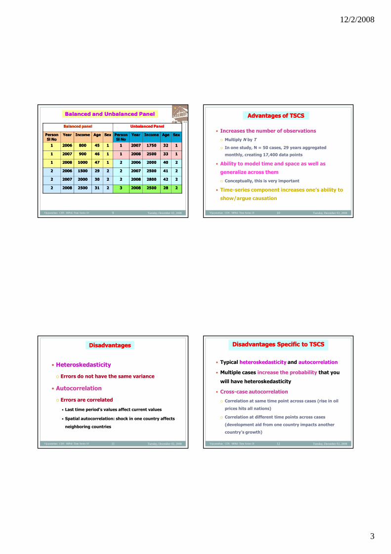
Balanced panelBalanced panel Unbalanced PanelUnbalanced Panel
PersonPersonSl NoSl No
YearYear IncomeIncome AgeAge SexSex PersonPersonSl NoSl No
YearYear IncomeIncome AgeAge SexSex
11 20062006 800800 4545 11 11 20072007 17501750 3232 11
11 20072007 900900 4646 11 11 20082008 25002500 3333 11
11 20082008 10001000 4747 11 22 20062006 20002000 4040 22
22 20062006 15001500 2929 22 22 20072007 25002500 4141 22
22 20072007 20002000 3030 22 22 20082008 28002800 4242 22
22 20082008 25002500 3131 22 33 20082008 25002500 2828 22
Balanced and Unbalanced PanelBalanced and Unbalanced Panel
Tuesday, December 02, 2008Vijayamohan: CDS MPhil: Time Series 10 10
Increases the number of observations
Multiply N by T
In one study, N = 50 cases, 29 years aggregated
monthly, creating 17,400 data points
Ability to model time and space as well as
generalize across them
Conceptually, this is very important
Time-series component increases one’s ability to
show/argue causation
Advantages of TSCSAdvantages of TSCS
Tuesday, December 02, 2008Vijayamohan: CDS MPhil: Time Series 10 11
Heteroskedasticity
Errors do not have the same variance
Autocorrelation
Errors are correlated
Last time period’s values affect current values
Spatial autocorrelation: shock in one country affects
neighboring countries
DisadvantagesDisadvantages
Tuesday, December 02, 2008Vijayamohan: CDS MPhil: Time Series 10 12
Typical heteroskedasticity and autocorrelation
Multiple cases increase the probability that you
will have heteroskedasticity
Cross-case autocorrelation
Correlation at same time point across cases (rise in oil
prices hits all nations)
Correlation at different time points across cases
(development aid from one country impacts another
country’s growth)
Disadvantages Specific to TSCSDisadvantages Specific to TSCS
12/2/2008
4
Tuesday, December 02, 2008Vijayamohan: CDS MPhil: Time Series 10 13
TheThe PanelPanel AnalysisAnalysis EquationEquation
TheThe equationequation explainingexplaining personalpersonal expendituresexpenditures mightmight
bebe expressedexpressed asas::
YYitit == ii ++ 11XX11itit ++ 22XX22itit ++ εεitit ;;
ForFor example,example,
PEPEitit == ii ++ 11HHYHHYitit ++ 22PDYPDYitit ++ εεitit ..
Tuesday, December 02, 2008Vijayamohan: CDS MPhil: Time Series 10 14
The model is generally written as:The model is generally written as:
yyitit == xxitit’’ ++ ii ++ uuitit ;;
uuitit IIN(0,IIN(0, 22); Cov(); Cov(xxitit,, uuitit) = 0;) = 0;
wherewhere yyitit is theis the dependent variabledependent variable,,
xxitit is theis the vector of regressorsvector of regressors,,
ββ is theis the vector of coefficientsvector of coefficients,, uuitit is theis the error termerror term
andand
ii == individual effectsindividual effects: captures effects of the: captures effects of the ii--thth
individualindividual--specific variablesspecific variables that are constantthat are constant
over time.over time.
Tuesday, December 02, 2008Vijayamohan: CDS MPhil: Time Series 10 15
TypesTypes ofof PanelPanel AnalyticAnalytic ModelsModels::
Several types of panel dataSeveral types of panel dataanalytic models:analytic models:
Constant Coefficients models,Constant Coefficients models,
Fixed Effects models,Fixed Effects models, andand
Random Effects models.Random Effects models.
Tuesday, December 02, 2008Vijayamohan: CDS MPhil: Time Series 10 16
Data taken from Grunfeld (1958)
Real gross investment (millions of dollars deflated by
implicit price deflator of producers’ durable equipment)
= f(Ft-1, Ct-1),
where Ft = Real value of the firm (share price times
number of shares plus total book value of debt; millions
of dollars deflated by implicit price deflator of GNP),
and
Ct = Real capital stock (accumulated sum of net
additions to plant and equipment, deflated by
depreciation expense deflator – 10 year moving
average of WPI of metals and metal products) Positive
relationship, a priori.
Estimation of Panel Data Regression ModelsEstimation of Panel Data Regression Models
12/2/2008
5
Tuesday, December 02, 2008Vijayamohan: CDS MPhil: Time Series 10 17
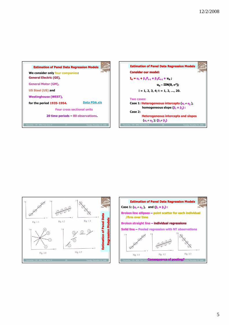
We consider only four companies:
General Electric (GE),
General Motor (GM),
US Steel (US) and
Westinghouse (WEST),
for the period 1935-1954.
Four cross sectional units
20 time periods – 80 observations.
Estimation of Panel Data Regression ModelsEstimation of Panel Data Regression Models
Data PDA.xls
Tuesday, December 02, 2008Vijayamohan: CDS MPhil: Time Series 10 18
Consider our model:Consider our model:
IIitit == ii ++ 11FFtt--11 ++ 22CCtt--11 ++ uuitit ;;
uuitit IIN(0,IIN(0, 22););
i = 1, 2, 3, 4; t = 1, 2, …, 20.
Two cases:
Case 1: Heterogeneous intercepts (ii jj ),
homogeneous slope (ii == jj) :) :
Case 2:
Heterogeneous intercepts and slopes
(ii jj ); (ii jj))
Estimation of Panel Data Regression ModelsEstimation of Panel Data Regression Models
Tuesday, December 02, 2008Vijayamohan: CDS MPhil: Time Series 10 19
Esti
ma
tio
no
fP
an
el
Da
taE
sti
ma
tio
no
fP
an
el
Da
ta
Re
gre
ssio
nM
od
els
Re
gre
ssio
nM
od
els
Tuesday, December 02, 2008Vijayamohan: CDS MPhil: Time Series 10 20
Case 1: (ii jj ), and (ii == jj)) ::
BrokenBroken line ellipsesline ellipses –– point scatter for eachpoint scatter for each individualindividual
//firmfirm over timeover time
BrokenBroken straight linestraight line –– individual regressionsindividual regressions
SolidSolid lineline –– Pooled regression with NT observationsPooled regression with NT observations
ConsequenceConsequence of pooling?of pooling?
Estimation of Panel Data Regression ModelsEstimation of Panel Data Regression Models
12/2/2008
6
Tuesday, December 02, 2008Vijayamohan: CDS MPhil: Time Series 10 21
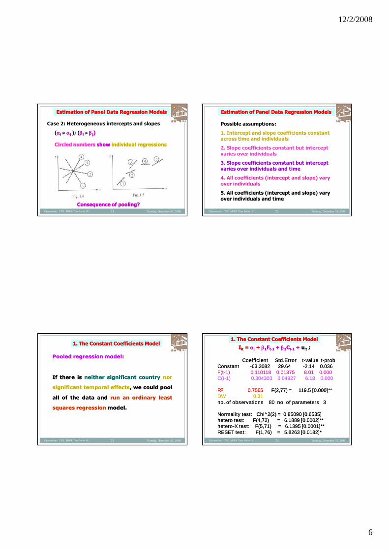
Case 2: Heterogeneous intercepts and slopes
(ii jj ); (ii jj))
Circled numbersCircled numbers showshow individual regressionsindividual regressions
ConsequenceConsequence of pooling?of pooling?
Estimation of Panel Data Regression ModelsEstimation of Panel Data Regression Models
Tuesday, December 02, 2008Vijayamohan: CDS MPhil: Time Series 10 22
Possible assumptions:
1. Intercept and slope coefficients constantacross time and individuals
2. Slope coefficients constant but interceptvaries over individuals
3. Slope coefficients constant but interceptvaries over individuals and time
4. All coefficients (intercept and slope) varyover individuals
5. All coefficients (intercept and slope) varyover individuals and time
Estimation of Panel Data Regression ModelsEstimation of Panel Data Regression Models
Tuesday, December 02, 2008Vijayamohan: CDS MPhil: Time Series 10 23
PooledPooled regressionregression modelmodel::
IfIf therethere isis neitherneither significantsignificant countrycountry nornor
significantsignificant temporaltemporal effectseffects,, wewe couldcould poolpool
allall ofof thethe datadata andand runrun anan ordinaryordinary leastleast
squaressquares regressionregression modelmodel..
1. The Constant Coefficients Model1. The Constant Coefficients Model
Tuesday, December 02, 2008Vijayamohan: CDS MPhil: Time Series 10 24
CoefficientCoefficient Std.ErrorStd.Error tt--value tvalue t--probprobConstantConstant --63.3082 29.6463.3082 29.64 --2.14 0.0362.14 0.036F(tF(t--1) 0.110118 0.01375 8.01 0.0001) 0.110118 0.01375 8.01 0.000C(tC(t--1) 0.304303 0.04927 6.18 0.0001) 0.304303 0.04927 6.18 0.000
RR22 0.75650.7565 F(2,77) = 119.5 [0.000]**F(2,77) = 119.5 [0.000]**DW 0.31DW 0.31no. of observations 80 no. of parameters 3no. of observations 80 no. of parameters 3
Normality test: Chi^2(2) = 0.85090 [0.6535]Normality test: Chi^2(2) = 0.85090 [0.6535]hetero test: F(4,72) = 6.1889 [0.0002]**hetero test: F(4,72) = 6.1889 [0.0002]**heterohetero--X test: F(5,71) = 6.1395 [0.0001]**X test: F(5,71) = 6.1395 [0.0001]**RESET test: F(1,76) = 5.8263 [0.0182]*RESET test: F(1,76) = 5.8263 [0.0182]*
1. The Constant Coefficients Model1. The Constant Coefficients Model
IIitit == ii ++ 11FFtt--11 ++ 22CCtt--11 ++ uuitit ;;

12/2/2008
7
Tuesday, December 02, 2008Vijayamohan: CDS MPhil: Time Series 10 25
No significant temporal effects,
But significant differences among companies.
That is, a linear regression model in which the
intercept terms vary over individual units:
yit = xit + i + uit ;
uit IIN(0, 2);
Cov(xit, uis) = 0; t and s
2. The Fixed Effects Model:2. The Fixed Effects Model:(Least Squares Dummy Variable Model):(Least Squares Dummy Variable Model):
Tuesday, December 02, 2008Vijayamohan: CDS MPhil: Time Series 10 26
yyitit == xxitit ++ ii ++ uuitit ;;
Possible toPossible to include a dummy variableinclude a dummy variable forfor eacheach
unitunit ii in the model:in the model:
yyitit == xxitit ++ iiddii ++ uuitit ;;
Four Companies:Four Companies:
Three dummiesThree dummies
Additive
2. The Fixed Effects Model:2. The Fixed Effects Model:
Constant Slope; Variable InterceptConstant Slope; Variable Intercept
Tuesday, December 02, 2008Vijayamohan: CDS MPhil: Time Series 10 27
yyitit == xxitit ++ iiddii ++ uuitit ;;
For example,For example,
YYitit ==11 ++22DD22ii ++33DD33ii ++44DD44ii ++ 11XX11itit ++ 22XX22itit ++ εεitit ;;
wherewhere DD22ii = 1 for GM; and= 1 for GM; and zero otherwisezero otherwise..
DD33ii = 1 for US; and= 1 for US; and zero otherwisezero otherwise..
DD44ii = 1 for WEST; and= 1 for WEST; and zero otherwisezero otherwise..
2 (a). The Fixed Effects Model:2 (a). The Fixed Effects Model:
Constant Slope; Intercept Variable over CompaniesConstant Slope; Intercept Variable over Companies
Tuesday, December 02, 2008Vijayamohan: CDS MPhil: Time Series 10 28
YYitit ==11 ++22DD22ii ++33DD33ii ++44DD44ii ++ 11XX11itit ++ 22XX22itit ++ εεitit ;;
Base company: GE
Intercept for GE = 11
If all s statistically significant, differential intercepts.
For example, if 11 and 22 significant,
intercept for GM = 11 ++22
2 (a). The Fixed Effects Model:2 (a). The Fixed Effects Model:
Constant Slope; Intercept Variable over CompaniesConstant Slope; Intercept Variable over Companies
12/2/2008
8
Tuesday, December 02, 2008Vijayamohan: CDS MPhil: Time Series 10 29
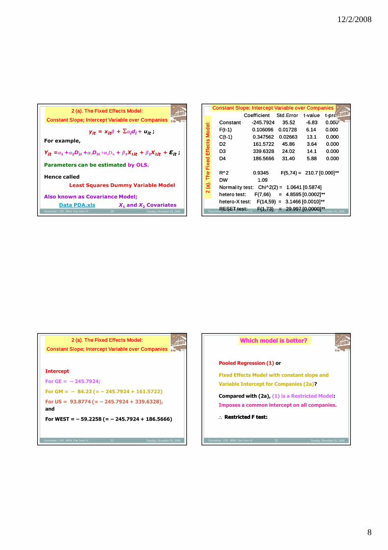
yit = xit + idi + uit ;
For example,
Yit =1 +2D2i +3D3i +4D4i + 1X1it + 2X2it + εit ;
Parameters can be estimated by OLS.
Hence called
Least Squares Dummy Variable Model
Also known as Covariance Model;
Data PDA.xls X1 and X2 Covariates
2 (a). The Fixed Effects Model:2 (a). The Fixed Effects Model:
Constant Slope; Intercept Variable over CompaniesConstant Slope; Intercept Variable over Companies
Tuesday, December 02, 2008Vijayamohan: CDS MPhil: Time Series 10 30
CoefficientCoefficient Std.ErrorStd.Error tt--value tvalue t--probprob
ConstantConstant --245.7924 35.52245.7924 35.52 --6.83 0.0006.83 0.000
F(tF(t--1) 0.106096 0.01728 6.14 0.0001) 0.106096 0.01728 6.14 0.000
C(tC(t--1) 0.347562 0.02663 13.1 0.0001) 0.347562 0.02663 13.1 0.000
D2 161.5722 45.86 3.64 0.000D2 161.5722 45.86 3.64 0.000
D3 339.6328 24.02 14.1 0.000D3 339.6328 24.02 14.1 0.000
D4 186.5666 31.40 5.88 0.000D4 186.5666 31.40 5.88 0.000
R^2 0.9345 F(5,74) = 210.7 [0.000]**R^2 0.9345 F(5,74) = 210.7 [0.000]**
DW 1.09DW 1.09
Normality test: Chi^2(2) = 1.0641 [0.5874]Normality test: Chi^2(2) = 1.0641 [0.5874]
hetero test: F(7,66) = 4.8595 [0.0002]**hetero test: F(7,66) = 4.8595 [0.0002]**
heterohetero--X test: F(14,59) = 3.1466 [0.0010]**X test: F(14,59) = 3.1466 [0.0010]**
RESET test: F(1,73) = 29.997 [0.0000]**RESET test: F(1,73) = 29.997 [0.0000]**2
(a).
Th
eF
ixe
dE
ffe
cts
Mo
de
l2
(a).
Th
eF
ixe
dE
ffe
cts
Mo
de
l::
ConstantConstant Slope; Intercept Variable over CompaniesSlope; Intercept Variable over Companies
Tuesday, December 02, 2008Vijayamohan: CDS MPhil: Time Series 10 31
Intercept
For GE = – 245.7924;
For GM = – 84.22 (= – 245.7924 + 161.5722)
For US = 93.8774 (= – 245.7924 + 339.6328),
and
For WEST = – 59.2258 (= – 245.7924 + 186.5666)
2 (a). The Fixed Effects Model:2 (a). The Fixed Effects Model:
Constant Slope; Intercept Variable over CompaniesConstant Slope; Intercept Variable over Companies
Tuesday, December 02, 2008Vijayamohan: CDS MPhil: Time Series 10 32
Pooled Regression (1) or
Fixed Effects Model with constant slope and
Variable Intercept for Companies (2a)?
Compared with (2a), (1) is a Restricted Model:
Imposes a common intercept on all companies.
Restricted F test:Restricted F test:
Which model is better?Which model is better?
12/2/2008
9
Tuesday, December 02, 2008Vijayamohan: CDS MPhil: Time Series 10 33
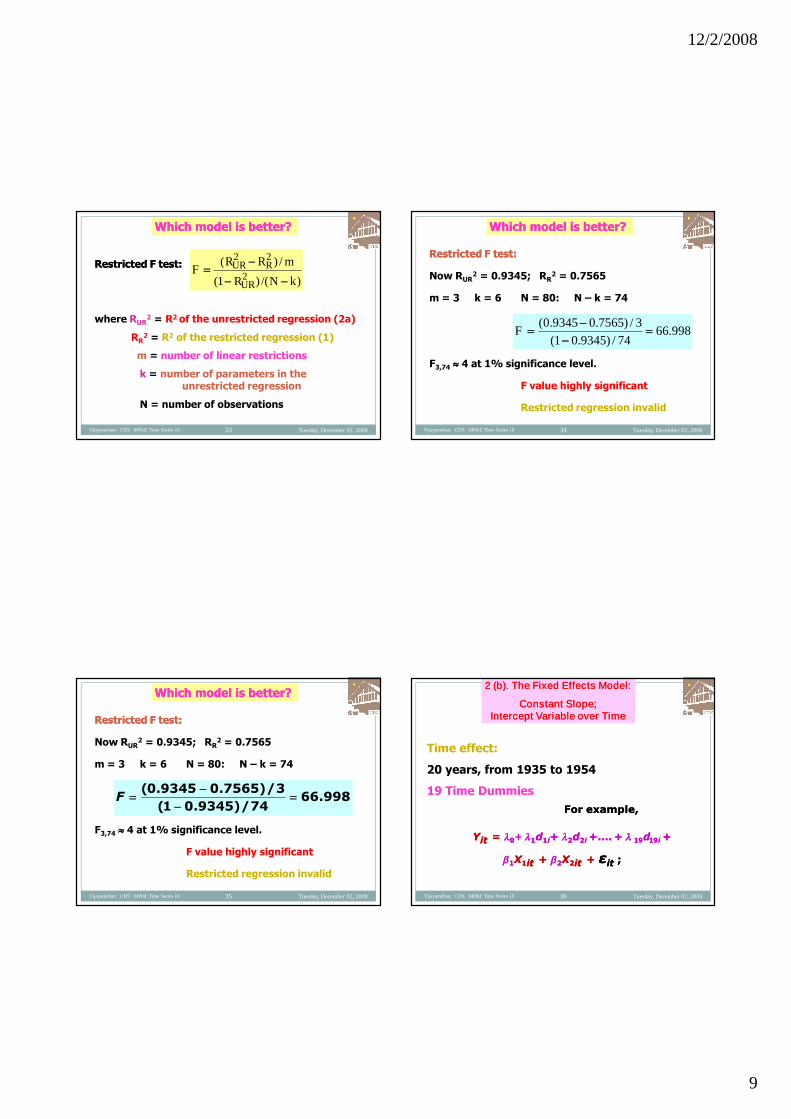
Restricted F test:Restricted F test:
where RUR2 = R2 of the unrestricted regression (2a)
RR2 = R2 of the restricted regression (1)
m = number of linear restrictions
k = number of parameters in theunrestricted regression
N = number of observations
)/()1(
/)(2
22
kNR
mRRF
UR
RUR
Which model is better?Which model is better?
Tuesday, December 02, 2008Vijayamohan: CDS MPhil: Time Series 10 34
Restricted F test:Restricted F test:
Now RUR2 = 0.9345; RR
2 = 0.7565
m = 3 k = 6 N = 80: N – k = 74
F3,74 4 at 1% significance level.
F value highly significant
Restricted regression invalid
998.6674/)9345.01(
3/)7565.09345.0(
F
Which model is better?Which model is better?
Tuesday, December 02, 2008Vijayamohan: CDS MPhil: Time Series 10 35
Restricted F test:Restricted F test:
Now RUR2 = 0.9345; RR
2 = 0.7565
m = 3 k = 6 N = 80: N – k = 74
F3,74 4 at 1% significance level.
F value highly significant
Restricted regression invalid
998.6674/)9345.01(
3/)7565.09345.0(
F
Which model is better?Which model is better?
Tuesday, December 02, 2008Vijayamohan: CDS MPhil: Time Series 10 36
Time effect:
20 years, from 1935 to 1954
19 Time Dummies
For example,For example,
YYitit == 00+ 11dd11ii++ 22dd22ii +….+…. ++ 1919dd1919ii ++
11XX11itit ++ 22XX22itit ++ εεitit ;;
2 (b). The Fixed Effects Model:2 (b). The Fixed Effects Model:
Constant Slope;Constant Slope;Intercept Variable over TimeIntercept Variable over Time

12/2/2008
10
Tuesday, December 02, 2008Vijayamohan: CDS MPhil: Time Series 10 37
YYitit == 00+ 11dd11ii++ 22dd22ii +….+…. ++ 1919dd1919ii ++
11XX11itit ++ 22XX22itit ++ εεitit ;;
where d1i = 1 for year 1935;
zero otherwise, etc.
Data PDA.xls 1954 as base year; intercept 00
2 (b). The Fixed Effects Model:2 (b). The Fixed Effects Model:
Constant Slope;Constant Slope;Intercept Variable over TimeIntercept Variable over Time
Tuesday, December 02, 2008Vijayamohan: CDS MPhil: Time Series 10 38
Coefficient Std.Error t-value t-probConstant -57.9001 99.73 -0.581 0.564F(t-1) 0.116091 0.01819 6.38 0.000C(t-1) 0.270715 0.08321 3.25 0.002d1 22.2924 129.7 0.172 0.864d2 -12.9191 133.1 -0.0970 0.923d3 -57.4624 135.1 -0.425 0.672d4 -47.5873 126.5 -0.376 0.708d5 -95.8224 127.9 -0.749 0.457d6 -35.1423 129.1 -0.272 0.786d7 22.1193 127.7 0.173 0.863d8 31.2809 124.1 0.252 0.802d9 -11.8292 124.8 -0.0948 0.925d10 -16.8720 125.6 -0.134 0.894d11 -38.0538 126.7 -0.300 0.765d12 27.7564 125.7 0.221 0.826d13 36.4606 119.2 0.306 0.761d14 26.8074 117.3 0.229 0.820d15 -27.9772 116.3 -0.241 0.811d16 -19.7576 115.9 -0.171 0.865d17 1.50284 116.2 0.0129 0.990d18 22.3616 114.7 0.195 0.846d19 39.5883 113.4 0.349 0.728
RR22 = 0.7697= 0.7697F(21,58) =F(21,58) = 9.272 [0.0009.272 [0.000]**]**DW = 0.263DW = 0.263
Normality test: Chi^2(2) =Normality test: Chi^2(2) =0.67046 [0.7152]0.67046 [0.7152]
hetero test: F(23,34) =hetero test: F(23,34) =1.37431.3743 [[0.1958]0.1958]
RESET test: F(1,57) =RESET test: F(1,57) =6.74806.7480 [[0.0119]*0.0119]*
2 (b). The Fixed Effects Model:2 (b). The Fixed Effects Model:
Constant Slope;Constant Slope; InterceptIntercept Variable over TimeVariable over Time
Tuesday, December 02, 2008Vijayamohan: CDS MPhil: Time Series 10 39
Pooled regression or Time effect Model?
R2 from 2(b): 0.7697
R2 from (1): 0.7565
Increment of only 0.0132:
F test does not reject:
Time effect Insignificant
Investment function has not changed much over
time
Which model is better?Which model is better?
Tuesday, December 02, 2008Vijayamohan: CDS MPhil: Time Series 10 40
Company effects statistically significant
Time effects not!
Our model is mis-specified?
Take into account
both company and time effects together.
Which model is better?Which model is better?
12/2/2008
11
Tuesday, December 02, 2008Vijayamohan: CDS MPhil: Time Series 10 41
00+ 11dd11ii++ 22dd22ii +….+…. ++ 1919dd1919ii ++
11XX11itit ++ 22XX22itit ++ εεitit ;;
YYitit ==11 ++22DD22ii ++33DD33ii ++44DD44ii ++
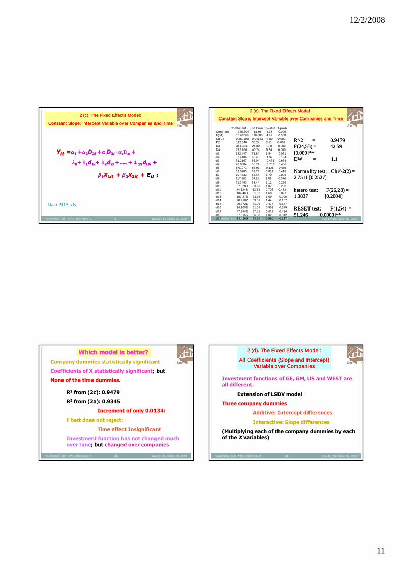
2 (c). The Fixed Effects Model:2 (c). The Fixed Effects Model:
Constant Slope;Constant Slope; InterceptIntercept Variable over Companies and TimeVariable over Companies and Time
Data PDA.xls
Tuesday, December 02, 2008Vijayamohan: CDS MPhil: Time Series 10 42
Coefficient Std.Error t-value t-probConstant -355.302 81.98 -4.33 0.000F(t-1) 0.126778 0.02688 4.72 0.000C(t-1) 0.369108 0.04153 8.89 0.000D2 112.546 36.24 3.11 0.003D3 341.364 24.80 13.8 0.000D4 217.696 40.74 5.34 0.000d1 132.447 71.84 1.84 0.071d2 87.4106 66.46 1.32 0.194d3 31.2167 66.04 0.473 0.638d4 46.8584 66.74 0.702 0.486d5 -8.01071 63.91 -0.125 0.901d6 52.0983 63.78 0.817 0.418d7 107.733 63.45 1.70 0.095d8 117.185 64.85 1.81 0.076d9 71.3493 63.44 1.12 0.266d10 67.9288 63.63 1.07 0.290d11 44.3243 62.83 0.706 0.483d12 104.468 61.82 1.69 0.097d13 107.276 63.36 1.69 0.096d14 90.4187 63.01 1.44 0.157d15 29.3721 61.96 0.474 0.637d16 34.1052 61.05 0.559 0.579d17 47.3542 57.51 0.823 0.414d18 57.5156 56.38 1.02 0.312d19 54.4169 54.99 0.990 0.327
R^2 = 0.9479R^2 = 0.9479F(24,55) = 42.59F(24,55) = 42.59[0.000]**[0.000]**DW = 1.1DW = 1.1
Normality test: Chi^2(2) =Normality test: Chi^2(2) =2.7511 [0.2527]2.7511 [0.2527]
hetero test: F(26,28) =hetero test: F(26,28) =1.38371.3837 [0.2004][0.2004]
RESET test: F(1,54) =RESET test: F(1,54) =51.24651.246 [0.0000]**[0.0000]**
2 (c). The Fixed Effects Model:2 (c). The Fixed Effects Model:
Constant Slope;Constant Slope; InterceptIntercept Variable over Companies and TimeVariable over Companies and Time
Tuesday, December 02, 2008Vijayamohan: CDS MPhil: Time Series 10 43
Company dummies statistically significant
Coefficients of X statistically significant; but
None of the time dummies.
R2 from (2c): 0.9479
R2 from (2a): 0.9345
Increment of only 0.0134:
F test does not reject:
Time effect Insignificant
Investment function has not changed muchover time; but changed over companies
Which model is better?Which model is better?
Tuesday, December 02, 2008Vijayamohan: CDS MPhil: Time Series 10 44
Investment functions of GE, GM, US and WEST areall different.
Extension of LSDV model
Three company dummies
Additive: Intercept differences
Interactive: Slope differences
(Multiplying each of the company dummies by eachof the X variables)
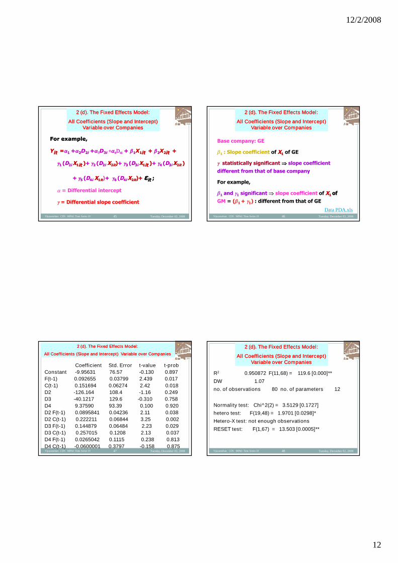
2 (d). The Fixed Effects Model:2 (d). The Fixed Effects Model:
All Coefficients (Slope and Intercept)All Coefficients (Slope and Intercept)Variable over CompaniesVariable over Companies
12/2/2008
12
Tuesday, December 02, 2008Vijayamohan: CDS MPhil: Time Series 10 45
For example,For example,
YYitit ==11 ++22DD22ii ++33DD33ii ++44DD44ii ++ 11XX11itit ++ 22XX22itit ++
11 ((DD22ii XX11itit ))++ 22 ((DD22ii XX22itit))++ 33 ((DD33ii XX11itit ))++ 44 ((DD33ii XX22itit ))
++ 55 ((DD44ii XX11itit)++ 66 ((DD44ii XX22itit)+)+ εεitit ;;
= Differential intercept
= Differential slope coefficient
2 (d). The Fixed Effects Model:2 (d). The Fixed Effects Model:
All Coefficients (Slope and Intercept)All Coefficients (Slope and Intercept)Variable over CompaniesVariable over Companies
Tuesday, December 02, 2008Vijayamohan: CDS MPhil: Time Series 10 46
Base company: GE
1 : Slope coefficient of XX11 of GE
statistically significant slope coefficient
different from that of base company
For example,
1 and 1 significant slope coefficient of XX11 ofof
GM = (1 + 1) : different from that of GE
2 (d). The Fixed Effects Model:2 (d). The Fixed Effects Model:
All Coefficients (Slope and Intercept)All Coefficients (Slope and Intercept)Variable over CompaniesVariable over Companies
Data PDA.xls
Tuesday, December 02, 2008Vijayamohan: CDS MPhil: Time Series 10 47
Coefficient Std. Error t-value t-prob
Constant -9.95631 76.57 -0.130 0.897
F(t-1) 0.092655 0.03799 2.439 0.017
C(t-1) 0.151694 0.06274 2.42 0.018
D2 -126.164 108.4 -1.16 0.249
D3 -40.1217 129.6 -0.310 0.758
D4 9.37590 93.39 0.100 0.920
D2 F(t-1) 0.0895841 0.04236 2.11 0.038
D2 C(t-1) 0.222211 0.06844 3.25 0.002
D3 F(t-1) 0.144879 0.06484 2.23 0.029
D3 C(t-1) 0.257015 0.1208 2.13 0.037
D4 F(t-1) 0.0265042 0.1115 0.238 0.813
D4 C(t-1) -0.0600001 0.3797 -0.158 0.875
2 (d). The Fixed Effects Model:2 (d). The Fixed Effects Model:
All Coefficients (Slope and Intercept) Variable over CompaniesAll Coefficients (Slope and Intercept) Variable over Companies
Tuesday, December 02, 2008Vijayamohan: CDS MPhil: Time Series 10 48
R2 0.950872 F(11,68) = 119.6 [0.000]**
DW 1.07
no. of observations 80 no. of parameters 12
Normality test: Chi^2(2) = 3.5129 [0.1727]
hetero test: F(19,48) = 1.9701 [0.0298]*
Hetero-X test: not enough observations
RESET test: F(1,67) = 13.503 [0.0005]**
2 (d). The Fixed Effects Model:2 (d). The Fixed Effects Model:
All Coefficients (Slope and Intercept)All Coefficients (Slope and Intercept)Variable over CompaniesVariable over Companies

12/2/2008
13
Tuesday, December 02, 2008Vijayamohan: CDS MPhil: Time Series 10 49
2 (d). The Fixed Effects Model:2 (d). The Fixed Effects Model:
All Coefficients (Slope and Intercept)All Coefficients (Slope and Intercept)Variable over CompaniesVariable over Companies
It is significantly related to Ft-1 and Ct-1
Slope coefficients of Base company (GE) significant
Both the slope coefficients significant for GM and US
But not for WEST
Tuesday, December 02, 2008Vijayamohan: CDS MPhil: Time Series 10 50
1. Too many regressors:
Numerically unattractive.
df ; error variance
Possibility of multicollinearity
2. Unable to identify the impact of time-
invariant variables (sex, colour, ethnicity,
education – invariant over time)
2. The Fixed Effects (LSDV) Model: Problems2. The Fixed Effects (LSDV) Model: Problems
Tuesday, December 02, 2008Vijayamohan: CDS MPhil: Time Series 10 51
3. Assumption that the error term follows classical
assumptions: uit ~ N(0, 2):
For a given period, possible that the error term for
GM is correlated with the error term for, say, US
or both US and WEST.
the Seemingly Unrelated Regression (SURE)Seemingly Unrelated Regression (SURE)
modellingmodelling (Arnold Zellner; see Jan Kmenta 1986
Elements of Econometrics)
2. The Fixed Effects (LSDV) Model: Problems2. The Fixed Effects (LSDV) Model: Problems
Tuesday, December 02, 2008Vijayamohan: CDS MPhil: Time Series 10 52
A Simple way:A Simple way:
TheThe same estimatorsame estimator forfor is obtainedis obtained if theif the
regressionregression is performedis performed inin deviations fromdeviations from
individual meansindividual means::
wherewhere
So we can writeSo we can write::
iiii xy
t iti yTy 1
).()( iitiitiit xxyy
2. The Fixed Effects (LSDV) Model: Problems2. The Fixed Effects (LSDV) Model: Problems
12/2/2008
14
Tuesday, December 02, 2008Vijayamohan: CDS MPhil: Time Series 10 53
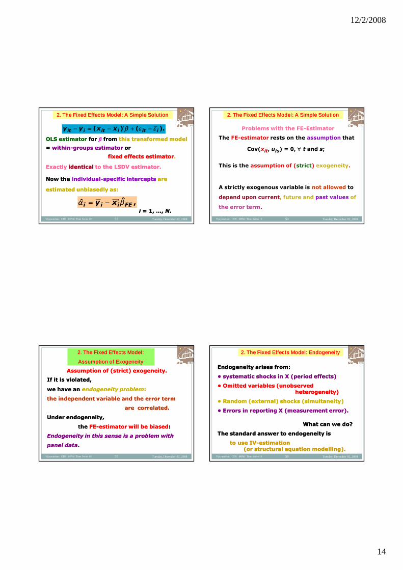
OLS estimatorOLS estimator forfor fromfrom this transformed modelthis transformed model
== withinwithin--groups estimatorgroups estimator oror
fixed effects estimatorfixed effects estimator..
ExactlyExactly identicalidentical to the LSDV estimator.to the LSDV estimator.
Now theNow the individualindividual--specific interceptsspecific intercepts areare
estimated unbiasedly as:estimated unbiasedly as:
ii = 1, …,= 1, …, NN..
,ˆˆ FEiii xy
).()( iitiitiit xxyy
2. The Fixed Effects Model: A Simple Solution2. The Fixed Effects Model: A Simple Solution
Tuesday, December 02, 2008Vijayamohan: CDS MPhil: Time Series 10 54
Problems with the FE-Estimator
The FE-estimator rests on the assumption that
Cov(xit, uis) = 0, t and s;
This is the assumption of (strict) exogeneity.
A strictly exogenous variable is not allowed to
depend upon current, future and past values of
the error term.
2. The Fixed Effects Model: A Simple Solution2. The Fixed Effects Model: A Simple Solution
Tuesday, December 02, 2008Vijayamohan: CDS MPhil: Time Series 10 55
Assumption of (strict) exogeneity.Assumption of (strict) exogeneity.
If it is violated,If it is violated,
we have anwe have an endogeneity problemendogeneity problem::
the independent variable and the error termthe independent variable and the error term
are correlated.are correlated.
Under endogeneity,Under endogeneity,
thethe FEFE--estimator will be biasedestimator will be biased::
Endogeneity in this sense is a problem withEndogeneity in this sense is a problem with
panel datapanel data..
2. The Fixed Effects Model:2. The Fixed Effects Model:
Assumption of ExogeneityAssumption of Exogeneity
Tuesday, December 02, 2008Vijayamohan: CDS MPhil: Time Series 10 56
Endogeneity arises from:Endogeneity arises from:
• systematic shocks in X (period effects)• systematic shocks in X (period effects)
• Omitted variables (unobserved• Omitted variables (unobservedheterogeneity)heterogeneity)
• Random (external) shocks (simultaneity)• Random (external) shocks (simultaneity)
• Errors in reporting X (measurement error).• Errors in reporting X (measurement error).
What can we do?What can we do?
The standard answer to endogeneity isThe standard answer to endogeneity is
to use IVto use IV--estimationestimation(or structural equation modelling).(or structural equation modelling).
2. The Fixed Effects Model: Endogeneity2. The Fixed Effects Model: Endogeneity
12/2/2008
15
Tuesday, December 02, 2008Vijayamohan: CDS MPhil: Time Series 10 57
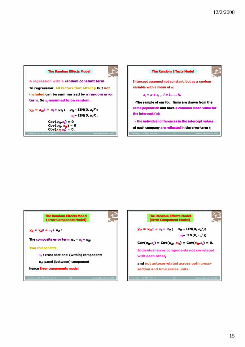
A regression with aA regression with a random constant termrandom constant term..
In regression:In regression: All factors that affectAll factors that affect yy butbut notnot
includedincluded can be summarized bycan be summarized by a random errora random error
termterm. So. So ii assumed to be random.assumed to be random.
yyitit == xxitit ++ ii ++ uuitit ;; uuitit IIN(0,IIN(0, uu22););
ii IIN(0,IIN(0, 22););
Cov(Cov(uuitit,,ii) = 0) = 0Cov(Cov(uuitit,, xxitit) = 0) = 0Cov(Cov(xxitit,,ii) = 0.) = 0.
The Random Effects ModelThe Random Effects Model
Tuesday, December 02, 2008Vijayamohan: CDS MPhil: Time Series 10 58
Intercept assumed not constant, but as a random
variable with a mean of :
ii = ++ ii ,, ii == 1, …,1, …, N.N.
TheThe sample of our four firms are drawn from thesample of our four firms are drawn from the
same populationsame population and haveand have a common mean value fora common mean value for
the intercept (the intercept (););
thethe individual differences in the intercept valuesindividual differences in the intercept values
of each companyof each company are reflectedare reflected in the error termin the error term ii
The Random Effects ModelThe Random Effects Model
Tuesday, December 02, 2008Vijayamohan: CDS MPhil: Time Series 10 59
yyitit == xxitit ++ ii ++ uuitit ;;
TheThe composite error termcomposite error term wwitit == ii ++ uuitit::
Two componentsTwo components::
ii : cross sectional (within) component;
uit: panel (between) component
hencehence Error components modelError components model
The Random Effects ModelThe Random Effects Model(Error Component Model)(Error Component Model)
Tuesday, December 02, 2008Vijayamohan: CDS MPhil: Time Series 10 60
yyitit == xxitit ++ ii ++ uuitit ;; uuitit IIN(0,IIN(0, uu22););
ii IIN(0,IIN(0, 22););
Cov(Cov(uuitit,,ii) = Cov() = Cov(uuitit,, xxitit) = Cov() = Cov(xxitit,,ii) = 0.) = 0.
Individual error components not correlatedIndividual error components not correlated
with each otherwith each other,,
andand not autocorrelated across both crossnot autocorrelated across both cross--
section and time series unitssection and time series units..
The Random Effects ModelThe Random Effects Model(Error Component Model)(Error Component Model)
12/2/2008
16
Tuesday, December 02, 2008Vijayamohan: CDS MPhil: Time Series 10 61
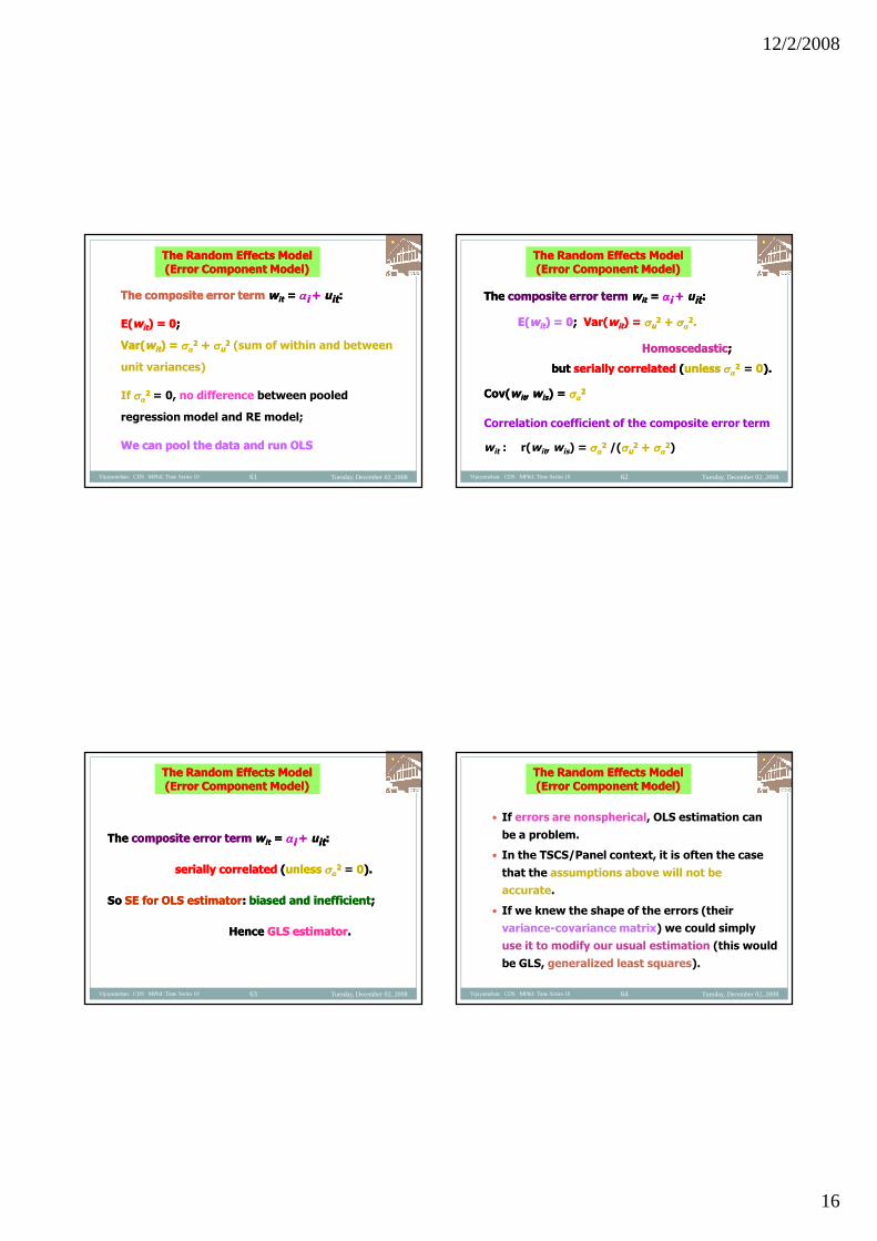
The composite error termThe composite error term wwitit == ii ++ uuitit::
E(E(wwitit) = 0) = 0;;
Var(Var(wwitit) =) = 22 ++ uu
22 (sum of within and between
unit variances)
If 22 = 0, no difference between pooled
regression model and RE model;
We can pool the data and run OLSWe can pool the data and run OLS
The Random Effects ModelThe Random Effects Model(Error Component Model)(Error Component Model)
Tuesday, December 02, 2008Vijayamohan: CDS MPhil: Time Series 10 62
TheThe composite error termcomposite error term wwitit == ii ++ uuitit::
E(E(wwitit) = 0) = 0;; Var(Var(wwitit) =) = uu22 ++
22..
HomoscedasticHomoscedastic;;
butbut serially correlatedserially correlated ((unlessunless 22 = 00).).
Cov(Cov(wwitit,, wwisis) =) = 22
Correlation coefficient of the composite error term
wit : r(wit, wis) = 22 /(uu
22 ++ 22)
The Random Effects ModelThe Random Effects Model(Error Component Model)(Error Component Model)
Tuesday, December 02, 2008Vijayamohan: CDS MPhil: Time Series 10 63
TheThe composite error termcomposite error term wwitit == ii ++ uuitit::
serially correlatedserially correlated ((unlessunless 22 = 00).).
SoSo SE for OLS estimatorSE for OLS estimator:: biased and inefficientbiased and inefficient;;
HenceHence GLS estimatorGLS estimator..
The Random Effects ModelThe Random Effects Model(Error Component Model)(Error Component Model)
Tuesday, December 02, 2008Vijayamohan: CDS MPhil: Time Series 10 64
If errors are nonspherical, OLS estimation can
be a problem.
In the TSCS/Panel context, it is often the case
that the assumptions above will not be
accurate.
If we knew the shape of the errors (their
variance-covariance matrix) we could simply
use it to modify our usual estimation (this would
be GLS, generalized least squares).
The Random Effects ModelThe Random Effects Model(Error Component Model)(Error Component Model)
12/2/2008
17
Tuesday, December 02, 2008Vijayamohan: CDS MPhil: Time Series 10 65
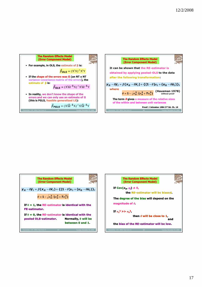
• For example, in OLS, the estimate of β is:
• If the shape of the errors was Ω (an NT x NTvariance-covariance matrix of the errors), theestimate of β is:
• In reality, we don’t know the shape of theerrors and we can only use an estimate of Ω(this is FGLS, feasible generalized LS):
YXXX -1)(OLS
YXXX 11ˆ -1)(GLS
YXXX 11 ˆˆˆ -1)(FGLS
The Random Effects ModelThe Random Effects Model(Error Component Model)(Error Component Model)
Tuesday, December 02, 2008Vijayamohan: CDS MPhil: Time Series 10 66
It can be shown that the RE-estimator is
obtained by applying pooled-OLS to the data
after the following transformation:
where
)},()1{()( iitiiitiit uuxxyy
)(1 222 Tuu
(Hausman 1978)without proof
Proof: J Johnston 1984 3Proof: J Johnston 1984 3rdrd Ed. Ch. 10Ed. Ch. 10
The Random Effects ModelThe Random Effects Model(Error Component Model)(Error Component Model)
The term θ gives a measure of the relative sizes
of the within and between unit variances
Tuesday, December 02, 2008Vijayamohan: CDS MPhil: Time Series 10 67
IfIf == 11, the, the RERE--estimatorestimator isis identical with theidentical with the
FEFE--estimatorestimator..
IfIf == 00, the, the RERE--estimatorestimator isis identical with theidentical with the
pooled OLSpooled OLS--estimatorestimator. Normally,. Normally, will bewill be
between 0 and 1between 0 and 1..
)},()1{()( iitiiitiit uuxxyy
)(1 222 Tuu
The Random Effects ModelThe Random Effects Model(Error Component Model)(Error Component Model)
Tuesday, December 02, 2008Vijayamohan: CDS MPhil: Time Series 10 68
IfIf Cov(Cov(xxitit,, ii)) ≠ 0,≠ 0,
thethe RERE--estimator will be biasedestimator will be biased..
TheThe degree of the biasdegree of the bias will depend on thewill depend on the
magnitude ofmagnitude of ..
IfIf 22 >>>> uu
22,,
thenthen will be close to 1will be close to 1,,andand
thethe bias of the REbias of the RE--estimator will be lowestimator will be low..
The Random Effects ModelThe Random Effects Model(Error Component Model)(Error Component Model)
12/2/2008
18
Tuesday, December 02, 2008Vijayamohan: CDS MPhil: Time Series 10 69
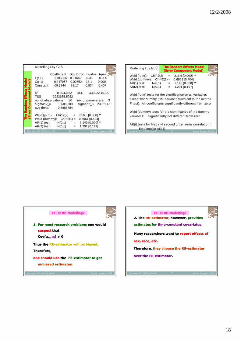
Modelling I by GLS
Coefficient Std. Error t-value t-probF(t-1) 0.105966 0.01662 6.38 0.000C(t-1) 0.347057 0.02652 13.1 0.000Constant -69.3944 83.17 -0.834 0.407
R2 0.8043662 RSS 435022.15199TSS 2223655.5252no. of observations 80 no. of parameters 3sigma^2_u 5685.389 sigma^2_ 23021.46avg theta 0.8888784
Wald (joint): Chi^2(2) = 316.6 [0.000] **Wald (dummy): Chi^2(1) = 0.6961 [0.404]AR(1) test: N(0,1) = 7.143 [0.000] **AR(2) test: N(0,1) = 1.291 [0.197]
Th
eR
an
do
mE
ffe
cts
Mo
de
lT
he
Ra
nd
om
Eff
ects
Mo
de
l(E
rro
rC
om
po
ne
nt
Mo
de
l)(E
rro
rC
om
po
ne
nt
Mo
de
l)
Tuesday, December 02, 2008Vijayamohan: CDS MPhil: Time Series 10 70
Modelling I by GLS
Wald (joint): Chi^2(2) = 316.6 [0.000] **Wald (dummy): Chi^2(1) = 0.6961 [0.404]AR(1) test: N(0,1) = 7.143 [0.000] **AR(2) test: N(0,1) = 1.291 [0.197]
Wald (joint) tests for the significance on all variables
except the dummy (Chi-square equivalent to the overall
F-test): All coefficients significantly different from zero
Wald (dummy) tests for the significance of the dummy
variables: Significantly not different from zero
AR(i) tests for first and second order serial correlation :
Evidence of AR(1)
The Random Effects ModelThe Random Effects Model(Error Component Model)(Error Component Model)
Tuesday, December 02, 2008Vijayamohan: CDS MPhil: Time Series 10 71
1.1. For most research problemsFor most research problems one wouldone would
suspectsuspect thatthat
Cov(Cov(xxitit,, ii) ≠ 0. ) ≠ 0.
Thus theThus the RERE--estimator will be biasedestimator will be biased..
Therefore,Therefore,
one should useone should use thethe FEFE--estimator to getestimator to get
unbiased estimates.unbiased estimates.
FEFE-- or REor RE--Modelling?Modelling?
Tuesday, December 02, 2008Vijayamohan: CDS MPhil: Time Series 10 72
2. The2. The RERE--estimatorestimator, however,, however, providesprovides
estimates forestimates for timetime--constant covariates.constant covariates.
Many researchers want toMany researchers want to report effects ofreport effects of
sex, race, etcsex, race, etc..
Therefore,Therefore, they choose the REthey choose the RE--estimatorestimator
over the FEover the FE--estimatorestimator..
FEFE-- or REor RE--Modelling?Modelling?

12/2/2008
19
Tuesday, December 02, 2008Vijayamohan: CDS MPhil: Time Series 10 73
Judge, GG, Hill, RC, Griffiths, WE, Lutkepohl, H andJudge, GG, Hill, RC, Griffiths, WE, Lutkepohl, H and
Lee, TSLee, TS (1988)(1988) Introduction to the Theory and PracticeIntroduction to the Theory and Practice
of Econometricsof Econometrics
1. If T is large and N small, little difference in the
parameter estimates of FE and RE models.
Computational convenience = FEM preferable
2. If N is large and T small, the two methods differ.
If cross-sectional units in the sample are random
drawings from a larger sample, REM appropriate;
if not, FEM.
FEFE-- or REor RE--Modelling?Modelling?
Tuesday, December 02, 2008Vijayamohan: CDS MPhil: Time Series 10 74
3. If the individual error component, I, and one or
more regressors are correlated, REM estimators
are biased; FEM estimators unbiased
4. If N is large and T small, and if the assumptions of
REM hold, REM estimators more efficient.
FEFE-- or REor RE--Modelling?Modelling?
Judge, GG, Hill, RC, Griffiths, WE, Lutkepohl, H andJudge, GG, Hill, RC, Griffiths, WE, Lutkepohl, H and
Lee, TSLee, TS (1988)(1988) Introduction to the Theory and PracticeIntroduction to the Theory and Practice
of Econometricsof Econometrics
Tuesday, December 02, 2008Vijayamohan: CDS MPhil: Time Series 10 75
In most applicationsIn most applications the assumptionthe assumption
Cov(Cov(xxitit,, ii) = 0) = 0 will be wrongwill be wrong,,
and theand the RERE--estimator will be biasedestimator will be biased..
This is risking to throw away the bigThis is risking to throw away the big
advantage of panel dataadvantage of panel data only to be able toonly to be able to
write a paperwrite a paper onon "The determinants of Y"."The determinants of Y".
(Josef Brüderl, 2005:(Josef Brüderl, 2005: Panel Data AnalysisPanel Data Analysis).).
However, we can have a test:However, we can have a test:
FEFE-- or REor RE--Modelling?Modelling?
Tuesday, December 02, 2008Vijayamohan: CDS MPhil: Time Series 10 76
The Hausman testThe Hausman test
The test evaluatesThe test evaluates
thethe significance of an estimatorsignificance of an estimator versusversus ananalternative estimator.alternative estimator.
In the linear model,In the linear model,
yy == bXbX ++ ee,,
yy isis univariateunivariate andandXX is ais a vector of regressorsvector of regressors,,
bb is ais a vector of coefficientsvector of coefficientsandand
ee isis the error termthe error term..
FEFE-- or REor RE--Modelling?Modelling?
12/2/2008
20
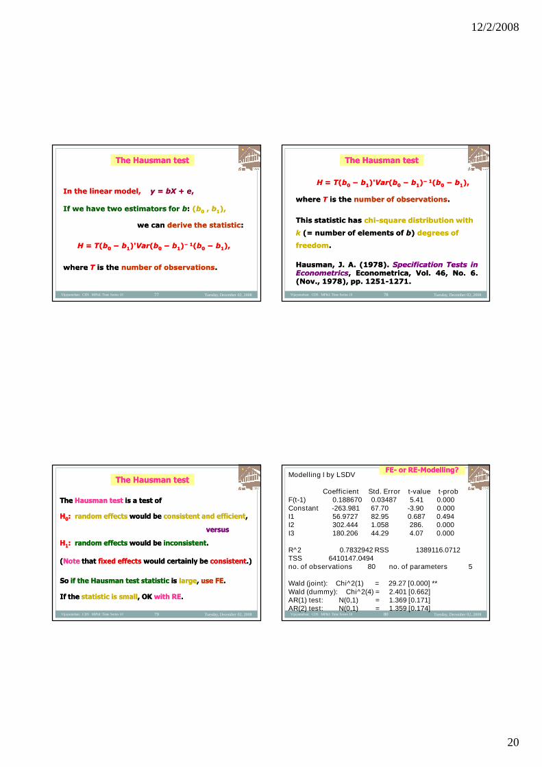
Tuesday, December 02, 2008Vijayamohan: CDS MPhil: Time Series 10 77
In the linear model,In the linear model, yy == bXbX ++ ee,,
If we have two estimators forIf we have two estimators for bb:: ((bb00 ,, bb11),),
we canwe can derive the statisticderive the statistic::
HH == TT((bb00 −− bb11)')'VarVar((bb00 −− bb11))− 1− 1((bb00 −− bb11),),
wherewhere TT is theis the number of observationsnumber of observations..
The Hausman testThe Hausman test
Tuesday, December 02, 2008Vijayamohan: CDS MPhil: Time Series 10 78
HH == TT((bb00 −− bb11)')'VarVar((bb00 −− bb11))− 1− 1((bb00 −− bb11),),
wherewhere TT is theis the number of observationsnumber of observations..
This statistic hasThis statistic has chichi--square distribution withsquare distribution with
kk (= number of elements of(= number of elements of bb)) degrees ofdegrees of
freedomfreedom..
Hausman,Hausman, JJ.. AA.. ((19781978)).. SpecificationSpecification TestsTests ininEconometricsEconometrics,, Econometrica,Econometrica, VolVol.. 4646,, NoNo.. 66..(Nov(Nov..,, 19781978),), pppp.. 12511251--12711271..
The Hausman testThe Hausman test
Tuesday, December 02, 2008Vijayamohan: CDS MPhil: Time Series 10 79
TheThe Hausman testHausman test is a test ofis a test of
HH00:: random effectsrandom effects would bewould be consistent and efficientconsistent and efficient,,
versusversus
HH11:: random effectsrandom effects would bewould be inconsistentinconsistent..
((NoteNote thatthat fixed effectsfixed effects would certainly bewould certainly be consistentconsistent.).)
SoSo if the Hausman test statisticif the Hausman test statistic isis largelarge,, use FEuse FE..
If theIf the statistic is smallstatistic is small, OK, OK with REwith RE..
The Hausman testThe Hausman test
Tuesday, December 02, 2008Vijayamohan: CDS MPhil: Time Series 10 80
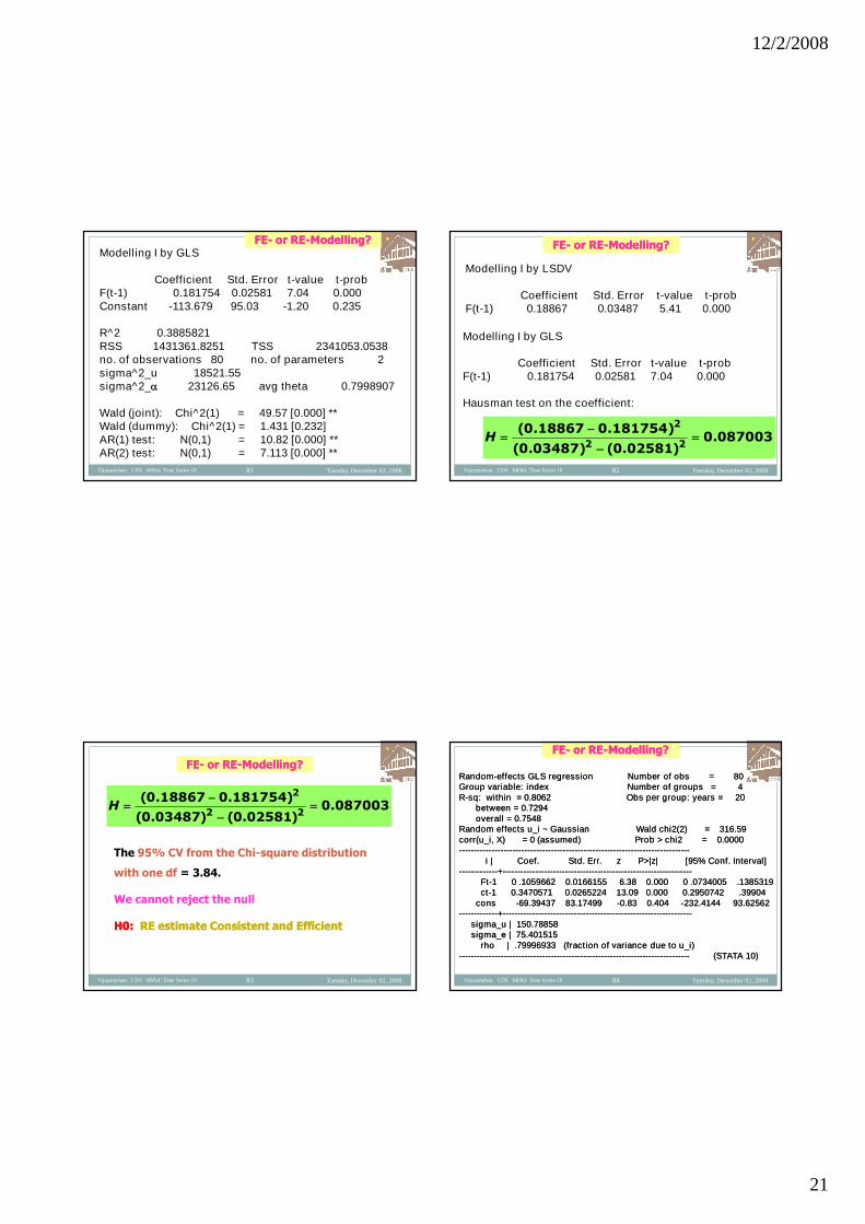
FEFE-- or REor RE--ModellingModelling??Modelling I by LSDV
Coefficient Std. Error t-value t-probF(t-1) 0.188670 0.03487 5.41 0.000Constant -263.981 67.70 -3.90 0.000I1 56.9727 82.95 0.687 0.494I2 302.444 1.058 286. 0.000I3 180.206 44.29 4.07 0.000
R^2 0.7832942 RSS 1389116.0712TSS 6410147.0494no. of observations 80 no. of parameters 5
Wald (joint): Chi^2(1) = 29.27 [0.000] **Wald (dummy): Chi^2(4) = 2.401 [0.662]AR(1) test: N(0,1) = 1.369 [0.171]AR(2) test: N(0,1) = 1.359 [0.174]
12/2/2008
21
Tuesday, December 02, 2008Vijayamohan: CDS MPhil: Time Series 10 81
Modelling I by GLS
Coefficient Std. Error t-value t-probF(t-1) 0.181754 0.02581 7.04 0.000Constant -113.679 95.03 -1.20 0.235
R^2 0.3885821RSS 1431361.8251 TSS 2341053.0538no. of observations 80 no. of parameters 2sigma^2_u 18521.55sigma^2_ 23126.65 avg theta 0.7998907
Wald (joint): Chi^2(1) = 49.57 [0.000] **Wald (dummy): Chi^2(1) = 1.431 [0.232]AR(1) test: N(0,1) = 10.82 [0.000] **AR(2) test: N(0,1) = 7.113 [0.000] **
FEFE-- or REor RE--ModellingModelling??
Tuesday, December 02, 2008Vijayamohan: CDS MPhil: Time Series 10 82
Modelling I by LSDV
Coefficient Std. Error t-value t-probF(t-1) 0.18867 0.03487 5.41 0.000
Modelling I by GLS
Coefficient Std. Error t-value t-probF(t-1) 0.181754 0.02581 7.04 0.000
Hausman test on the coefficient:
087003.0)02581.0()03487.0(
)181754.018867.0(22
2
H
FEFE-- or REor RE--ModellingModelling??
Tuesday, December 02, 2008Vijayamohan: CDS MPhil: Time Series 10 83
087003.0)02581.0()03487.0(
)181754.018867.0(22
2
H
The 95% CV from the Chi-square distribution
with one df = 3.84.
We cannot reject the null
H0:H0: RE estimate Consistent and EfficientRE estimate Consistent and Efficient
FEFE-- or REor RE--Modelling?Modelling?
Tuesday, December 02, 2008Vijayamohan: CDS MPhil: Time Series 10 84
FEFE-- or REor RE--Modelling?Modelling?
RandomRandom--effects GLS regression Number of obs = 80effects GLS regression Number of obs = 80Group variable: index Number of groups = 4Group variable: index Number of groups = 4RR--sq: within = 0.8062 Obs per group: years = 20sq: within = 0.8062 Obs per group: years = 20
between = 0.7294between = 0.7294overall = 0.7548overall = 0.7548
Random effects u_i ~ Gaussian Wald chi2(2) = 316.59Random effects u_i ~ Gaussian Wald chi2(2) = 316.59corr(u_i, X) = 0 (assumed) Prob > chi2 = 0.0000corr(u_i, X) = 0 (assumed) Prob > chi2 = 0.0000------------------------------------------------------------------------------------------------------------------------------------------------------------
i | Coef. Std. Err. z P>|z| [95% Conf.i | Coef. Std. Err. z P>|z| [95% Conf. Interval]Interval]--------------------------++--------------------------------------------------------------------------------------------------------------------------------
FtFt--1 0 .1059662 0.0166155 6.38 0.000 0 .0734005 .13853191 0 .1059662 0.0166155 6.38 0.000 0 .0734005 .1385319ctct--1 0.3470571 0.0265224 13.09 0.000 0.2950742 .399041 0.3470571 0.0265224 13.09 0.000 0.2950742 .39904
conscons --69.39437 83.1749969.39437 83.17499 --0.83 0.4040.83 0.404 --232.4144 93.62562232.4144 93.62562--------------------------++--------------------------------------------------------------------------------------------------------------------------------
sigma_u | 150.78858sigma_u | 150.78858sigma_e | 75.401515sigma_e | 75.401515
rho | .79996933 (fraction of variance due to u_i)rho | .79996933 (fraction of variance due to u_i)------------------------------------------------------------------------------------------------------------------------------------------------------------ (STATA 10)(STATA 10)
12/2/2008
22
Tuesday, December 02, 2008Vijayamohan: CDS MPhil: Time Series 10 85
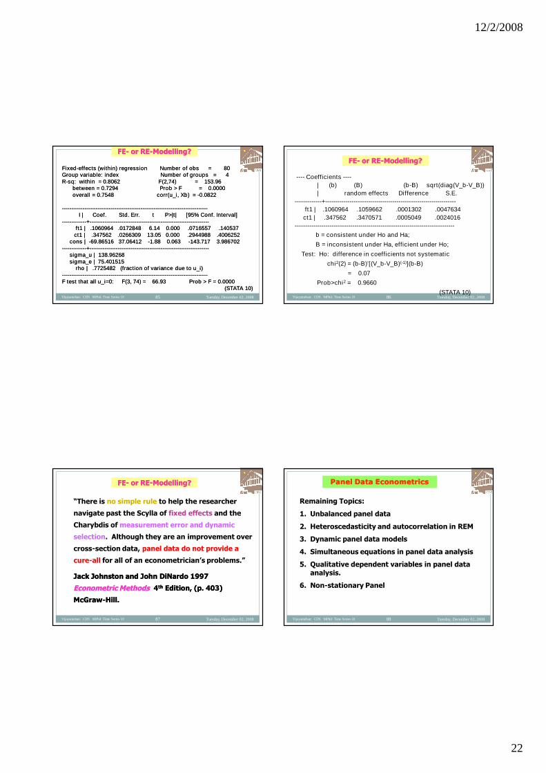
FEFE-- or REor RE--Modelling?Modelling?
FixedFixed--effects (within) regression Number of obs = 80effects (within) regression Number of obs = 80Group variable: index Number of groups = 4Group variable: index Number of groups = 4RR--sq: within = 0.8062 F(2,74) = 153.96sq: within = 0.8062 F(2,74) = 153.96
between = 0.7294between = 0.7294 Prob > F = 0.0000Prob > F = 0.0000overall = 0.7548overall = 0.7548 corr(u_i, Xb) =corr(u_i, Xb) = --0.08220.0822
------------------------------------------------------------------------------------------------------------------------------------------------------------I | Coef.I | Coef. Std. Err. t P>|t| [95% Conf.Std. Err. t P>|t| [95% Conf. Interval]Interval]
--------------------------++--------------------------------------------------------------------------------------------------------------------------------ft1 | .1060964 .0172848 6.14 0.000 .0716557 .140537ft1 | .1060964 .0172848 6.14 0.000 .0716557 .140537
ct1 | .347562 .0266309 13.05 0.000 .2944988 .4006252ct1 | .347562 .0266309 13.05 0.000 .2944988 .4006252cons |cons | --69.86516 37.0641269.86516 37.06412 --1.88 0.0631.88 0.063 --143.717 3.986702143.717 3.986702
--------------------------++--------------------------------------------------------------------------------------------------------------------------------sigma_u | 138.96268sigma_u | 138.96268sigma_e | 75.401515sigma_e | 75.401515
rho | .7725482 (fraction of variance due to u_i)rho | .7725482 (fraction of variance due to u_i)------------------------------------------------------------------------------------------------------------------------------------------------------------F test that all u_i=0: F(3, 74) = 66.93 Prob > F = 0.0000F test that all u_i=0: F(3, 74) = 66.93 Prob > F = 0.0000
(STATA 10)(STATA 10)
Tuesday, December 02, 2008Vijayamohan: CDS MPhil: Time Series 10 86
FEFE-- or REor RE--Modelling?Modelling?
---- Coefficients ----
| (b) (B) (b-B) sqrt(diag(V_b-V_B))
| random effects Difference S.E.
-------------+----------------------------------------------------------------
ft1 | .1060964 .1059662 .0001302 .0047634
ct1 | .347562 .3470571 .0005049 .0024016
------------------------------------------------------------------------------
b = consistent under Ho and Ha;
B = inconsistent under Ha, efficient under Ho;
Test: Ho: difference in coefficients not systematic
chi2(2) = (b-B)'[(V_b-V_B)(-1)](b-B)
= 0.07
Prob>chi2 = 0.9660
(STATA 10)
Tuesday, December 02, 2008Vijayamohan: CDS MPhil: Time Series 10 87
“There is no simple rule to help the researcher
navigate past the Scylla of fixed effects and the
Charybdis of measurement error and dynamic
selection. Although they are an improvement over
cross-section data, panel data do not provide a
cure-all for all of an econometrician’s problems.”
Jack Johnston and JohnJack Johnston and John DiNardoDiNardo 19971997
Econometric MethodsEconometric Methods 44thth Edition, (p. 403)Edition, (p. 403)
McGrawMcGraw--Hill.Hill.
FEFE-- or REor RE--Modelling?Modelling?
Tuesday, December 02, 2008Vijayamohan: CDS MPhil: Time Series 10 88
Remaining Topics:
1. Unbalanced panel data
2. Heteroscedasticity and autocorrelation in REM
3. Dynamic panel data models
4. Simultaneous equations in panel data analysis
5. Qualitative dependent variables in panel dataanalysis.
6. Non-stationary Panel
Panel Data EconometricsPanel Data Econometrics
12/2/2008
23
Tuesday, December 02,2008
Vijayamohan: CDS MPhil: TimeSeries 10
89


![[S.o. pillai] objective_physics_for_medical_and_e(book_fi.org)](https://img.pdfslide.us/doc/110x75/555f2609d8b42a93658b4f8a/so-pillai-objectivephysicsformedicalandebookfiorg.jpg)