��������� ����� � ������������������� ����� � ���! �"��� �#� � �%$'&)(*�+���-,.�)/��#�����0��)�)�

Vijay S. Kumar, Benjamin Rutt, Tahsin Kurc,Umit Catalyurek, Joel Saltz

Department of Biomedical InformaticsThe Ohio State University

Sunny Chow, Stephan Lamont, Maryann MartoneNational Center for Microscopy

and Imaging ResearchUniversity of California San Diego

13254�6�7�8�9:6

This paper is concerned with efficient execution of a pipelineof data processing operations on very large images obtainedfrom confocal microscopy instruments. We describe paral-lel, out-of-core algorithms for each operation in this pipeline.One of the challenging steps in the pipeline is the warpingoperation using inverse mapping based methods. We pro-pose and investigate a set of algorithms to handle the warpingcomputations on storage clusters. Our experimental resultsshow that the proposed approaches are scalable both in termsof number of processors and the size of images.

Keywords: imaging, digital microscopy, parallel computa-tion, PC clusters, out-of-core, warping

; <>= 6!7�?A@CBD9:6FEG? =

Biomedical imaging has proven to be one of the key clini-cal components in diagnosis and staging of complex diseasesand in the assessment of effectiveness of treatment regimens.Advances in imaging technologies such as digital confo-cal microscopy and digital high power light microscopy aremaking a dramatic impact on our ability to characterize dis-ease at the cellular and microscopic levels. Scanner tech-nologies for digitizing tissue samples and microscopy slideshave rapidly advanced in the past decade. Advanced scan-ners have been developed that are capable of capturing highresolution images rapidly1. As a result, digital imaging ofpathology slides and analysis of digitized microscopy im-ages have gained an increasing interest in many fields ofbiomedicine. However, a significant challenge is the efficientstorage, retrieval, and processing of the very large volumesof data required to represent a slide and a large collection ofslides. High resolution scanners can capture images of sin-gle slides at 150K H 150K pixels (66 Gigabytes). Process-ing of digital microscopy images involve a range of opera-

Permission to make digital or hard copies of all or part of this work forpersonal or classroom use is granted without fee provided that copies arenot made or distributed for profit or commercial advantage and that copiesbear this notice and the full citation on the first page. To copy otherwise, torepublish, to post on servers or to redistribute to lists, requires prior specificpermission and/or a fee.

SC2006 November 2006, Tampa, Florida, USA0-7695-2700-0/06 $20.00 c

I2006 IEEE

1Such scanners are being commercially produced

tions including simple 2D browsing of images, calculationof signal (color value) distribution within a sub-region of theimage, extraction of features through segmentation of differ-ent cell types, and 3D reconstruction of images from multi-ple slides, each of which represents a different focal plane.The memory and processing requirements of large volumesof image data make analysis of digitized microscopy imagesgood candidates for execution on parallel machines.

In an ongoing project, we are developing parallel runtimesupport for a pipeline of image processing operations on verylarge microscopy images. The purpose of this pipeline isto pre-process digitized images obtained from mouse braintissue samples using confocal microscopy instruments. Theoutput from this pipeline can be queried and analyzed usingadditional analysis methods. The pipeline consists of twomain stages; correctional tasks and preprocessing tasks (seeFigure 1). In our earlier work, we developed task- and data-parallel out-of-core algorithms for the pre-processing tasksstage [Rutt et al. 2005].

In this paper, we describe algorithms to efficiently executethe correctional tasks stage of the pipeline on parallel ma-chines and on very large images. This stage is composed of anetwork of tasks (see Figure 2). We have developed parallel,out-of-core algorithms for each task. The most challengingtask in this stage of the pipeline is warping. We employ awarping technique based on the inverse mapping approach.In this technique, pixels in the output image are traversedin a pre-determined order; for each output pixel the corre-sponding input pixel is obtained (using an inverse mappingfunction); and the color value of the output pixel is updatedusing the color value of the respective input pixel. For verylarge images and on parallel machines, this type of warpingalgorithm can result in high I/O and communication costs,because of the irregular mappings from the output imagespace to the input image space. We propose several algo-rithms to execute the warping task efficiently. We evaluateour algorithms using a PC cluster and multi-gigabyte largeimages. We also show that our approach is scalable to verylarge datasets using a synthetically generated 1-Terabyte im-age. Image warping can be employed in other imaging ap-plications such as remote sensing and satellite imagery. Ourproposed algorithms can also be applied in those applica-tions.

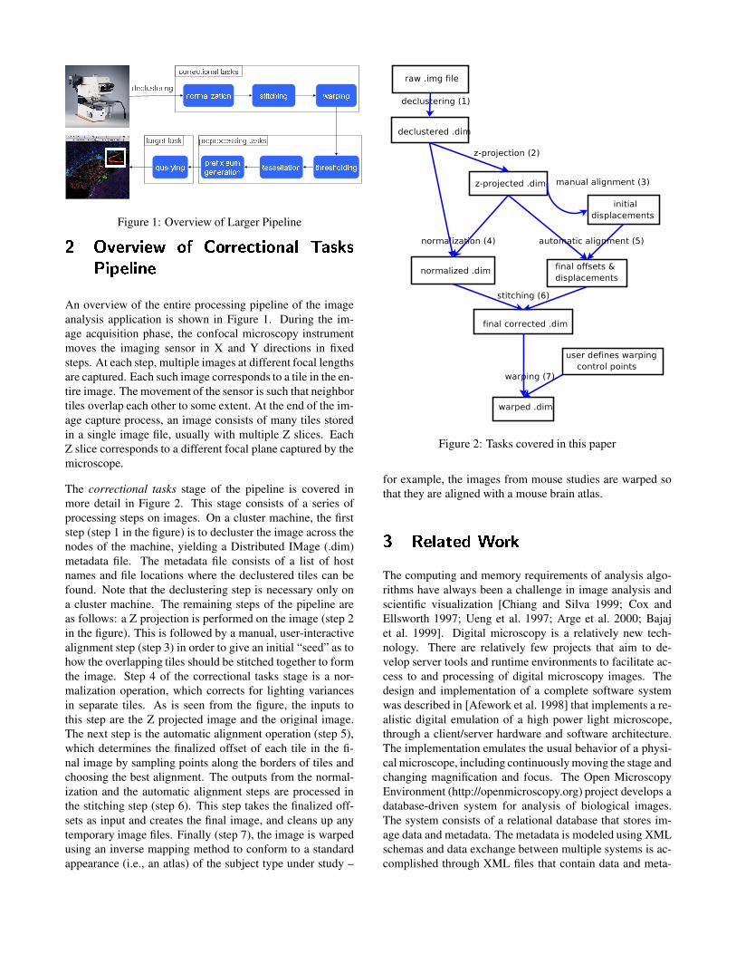
Figure 1: Overview of Larger PipelineJ KML*N 7 L E NPO ?RQTS0?R7U7 N 9:6FEG? = 8WVYX)8�4�ZP4[�E]\ N V^E =DN

An overview of the entire processing pipeline of the imageanalysis application is shown in Figure 1. During the im-age acquisition phase, the confocal microscopy instrumentmoves the imaging sensor in X and Y directions in fixedsteps. At each step, multiple images at different focal lengthsare captured. Each such image corresponds to a tile in the en-tire image. The movement of the sensor is such that neighbortiles overlap each other to some extent. At the end of the im-age capture process, an image consists of many tiles storedin a single image file, usually with multiple Z slices. EachZ slice corresponds to a different focal plane captured by themicroscope.

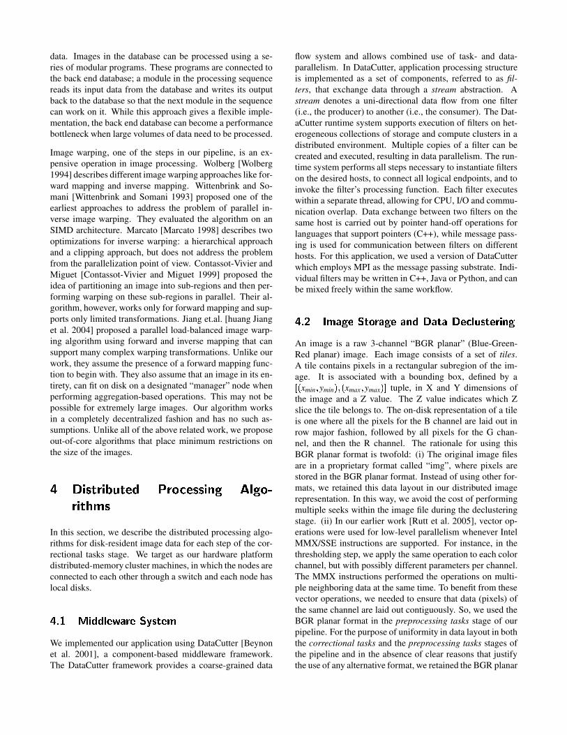
The correctional tasks stage of the pipeline is covered inmore detail in Figure 2. This stage consists of a series ofprocessing steps on images. On a cluster machine, the firststep (step 1 in the figure) is to decluster the image across thenodes of the machine, yielding a Distributed IMage (.dim)metadata file. The metadata file consists of a list of hostnames and file locations where the declustered tiles can befound. Note that the declustering step is necessary only ona cluster machine. The remaining steps of the pipeline areas follows: a Z projection is performed on the image (step 2in the figure). This is followed by a manual, user-interactivealignment step (step 3) in order to give an initial “seed” as tohow the overlapping tiles should be stitched together to formthe image. Step 4 of the correctional tasks stage is a nor-malization operation, which corrects for lighting variancesin separate tiles. As is seen from the figure, the inputs tothis step are the Z projected image and the original image.The next step is the automatic alignment operation (step 5),which determines the finalized offset of each tile in the fi-nal image by sampling points along the borders of tiles andchoosing the best alignment. The outputs from the normal-ization and the automatic alignment steps are processed inthe stitching step (step 6). This step takes the finalized off-sets as input and creates the final image, and cleans up anytemporary image files. Finally (step 7), the image is warpedusing an inverse mapping method to conform to a standardappearance (i.e., an atlas) of the subject type under study –

Figure 2: Tasks covered in this paper

for example, the images from mouse studies are warped sothat they are aligned with a mouse brain atlas.

_ `aN Vb8c6 N @ed�?W7UZ

The computing and memory requirements of analysis algo-rithms have always been a challenge in image analysis andscientific visualization [Chiang and Silva 1999; Cox andEllsworth 1997; Ueng et al. 1997; Arge et al. 2000; Bajajet al. 1999]. Digital microscopy is a relatively new tech-nology. There are relatively few projects that aim to de-velop server tools and runtime environments to facilitate ac-cess to and processing of digital microscopy images. Thedesign and implementation of a complete software systemwas described in [Afework et al. 1998] that implements a re-alistic digital emulation of a high power light microscope,through a client/server hardware and software architecture.The implementation emulates the usual behavior of a physi-cal microscope, including continuously moving the stage andchanging magnification and focus. The Open MicroscopyEnvironment (http://openmicroscopy.org) project develops adatabase-driven system for analysis of biological images.The system consists of a relational database that stores im-age data and metadata. The metadata is modeled using XMLschemas and data exchange between multiple systems is ac-complished through XML files that contain data and meta-

data. Images in the database can be processed using a se-ries of modular programs. These programs are connected tothe back end database; a module in the processing sequencereads its input data from the database and writes its outputback to the database so that the next module in the sequencecan work on it. While this approach gives a flexible imple-mentation, the back end database can become a performancebottleneck when large volumes of data need to be processed.

Image warping, one of the steps in our pipeline, is an ex-pensive operation in image processing. Wolberg [Wolberg1994] describes different image warping approaches like for-ward mapping and inverse mapping. Wittenbrink and So-mani [Wittenbrink and Somani 1993] proposed one of theearliest approaches to address the problem of parallel in-verse image warping. They evaluated the algorithm on anSIMD architecture. Marcato [Marcato 1998] describes twooptimizations for inverse warping: a hierarchical approachand a clipping approach, but does not address the problemfrom the parallelization point of view. Contassot-Vivier andMiguet [Contassot-Vivier and Miguet 1999] proposed theidea of partitioning an image into sub-regions and then per-forming warping on these sub-regions in parallel. Their al-gorithm, however, works only for forward mapping and sup-ports only limited transformations. Jiang et.al. [huang Jianget al. 2004] proposed a parallel load-balanced image warp-ing algorithm using forward and inverse mapping that cansupport many complex warping transformations. Unlike ourwork, they assume the presence of a forward mapping func-tion to begin with. They also assume that an image in its en-tirety, can fit on disk on a designated “manager” node whenperforming aggregation-based operations. This may not bepossible for extremely large images. Our algorithm worksin a completely decentralized fashion and has no such as-sumptions. Unlike all of the above related work, we proposeout-of-core algorithms that place minimum restrictions onthe size of the images.

f ghEG4�6�7iE]2jB�6 N @ [k7�?A9 N 4F4lE =�m 13V m ?Dn7iEb6�oqpr4

In this section, we describe the distributed processing algo-rithms for disk-resident image data for each step of the cor-rectional tasks stage. We target as our hardware platformdistributed-memory cluster machines, in which the nodes areconnected to each other through a switch and each node haslocal disks.

sPtGu vxwzy:y:{}|F~��!��|M���F����|��We implemented our application using DataCutter [Beynonet al. 2001], a component-based middleware framework.The DataCutter framework provides a coarse-grained data

flow system and allows combined use of task- and data-parallelism. In DataCutter, application processing structureis implemented as a set of components, referred to as fil-ters, that exchange data through a stream abstraction. Astream denotes a uni-directional data flow from one filter(i.e., the producer) to another (i.e., the consumer). The Dat-aCutter runtime system supports execution of filters on het-erogeneous collections of storage and compute clusters in adistributed environment. Multiple copies of a filter can becreated and executed, resulting in data parallelism. The run-time system performs all steps necessary to instantiate filterson the desired hosts, to connect all logical endpoints, and toinvoke the filter’s processing function. Each filter executeswithin a separate thread, allowing for CPU, I/O and commu-nication overlap. Data exchange between two filters on thesame host is carried out by pointer hand-off operations forlanguages that support pointers (C++), while message pass-ing is used for communication between filters on differenthosts. For this application, we used a version of DataCutterwhich employs MPI as the message passing substrate. Indi-vidual filters may be written in C++, Java or Python, and canbe mixed freely within the same workflow.

sPt�� �����l��|��+�������l��|h����y�����������|��F{��!����|���wb���An image is a raw 3-channel “BGR planar” (Blue-Green-Red planar) image. Each image consists of a set of tiles.A tile contains pixels in a rectangular subregion of the im-age. It is associated with a bounding box, defined by a�}�

xmin   ymin ¡�  � xmax   ymax ¡G¢ tuple, in X and Y dimensions ofthe image and a Z value. The Z value indicates which Zslice the tile belongs to. The on-disk representation of a tileis one where all the pixels for the B channel are laid out inrow major fashion, followed by all pixels for the G chan-nel, and then the R channel. The rationale for using thisBGR planar format is twofold: (i) The original image filesare in a proprietary format called “img”, where pixels arestored in the BGR planar format. Instead of using other for-mats, we retained this data layout in our distributed imagerepresentation. In this way, we avoid the cost of performingmultiple seeks within the image file during the declusteringstage. (ii) In our earlier work [Rutt et al. 2005], vector op-erations were used for low-level parallelism whenever IntelMMX/SSE instructions are supported. For instance, in thethresholding step, we apply the same operation to each colorchannel, but with possibly different parameters per channel.The MMX instructions performed the operations on multi-ple neighboring data at the same time. To benefit from thesevector operations, we needed to ensure that data (pixels) ofthe same channel are laid out contiguously. So, we used theBGR planar format in the preprocessing tasks stage of ourpipeline. For the purpose of uniformity in data layout in boththe correctional tasks and the preprocessing tasks stages ofthe pipeline and in the absence of clear reasons that justifythe use of any alternative format, we retained the BGR planar

format for this paper.

The tiles are then stored in multiple files or multiple contigu-ous regions of one or more files on disk. A tile represents theunit of I/O. On a cluster system, tiles are declustered acrossfiles stored on different compute nodes. A compute node“owns” a particular set of tiles, if the compute node has thetile data available on local disk.

The first step in our pipeline is declustering; that is, convert-ing a single image file into a distributed image file consistingof tiles spread across compute nodes. Some of the opera-tions such as the automated alignment step in the pipelineneed access to neighbor tiles during execution. In order tominimize inter-processor communication in such steps, theneighbor tiles are grouped to form blocks. A block consistsof a subset of tiles that are neighbors in X and Y dimensionsof the image. All the tiles that have the same bounding box,but different Z values are assigned to the same block. That is,the raw image captured by the microscope is partitioned in Xand Y dimensions, but not in Z dimension. A tile is assignedto a single block, and a block is stored on only one node.The blocks are declustered across the nodes in the system inround-robin fashion. A node may store multiple blocks.

sPt�£ ¤q�+�.���+�h��|F�a��¥)¦�w�{§��|����

For each step of the processing pipeline, we have imple-mented filters that are specific to processing applied in thatstep. There are also a set of filters that are common to allsteps and provide support for reading and writing distributedimages. The mediator filter provides a common mechanismto read a tile from an input image, regardless of whether itis on local or remote disk. It also provides a means to writeout a new tile on local disk for an image currently being cre-ated, and a mechanism to finalize all written tiles at once intotheir final output directories, such that total success or totalfailure in writing a new image transpires. The mediator fil-ter receives requests from client filters and works with othermediator filters on other compute nodes to carry out inputtile requests. The actual I/O to a local filesystem is delegatedto a mediator reader filter, which receives requests from themediator on the same compute node. The rangefetcher fil-ter is used to hide data retrieval latency. It issues a seriesof requests on behalf of its client filter to fetch a numberof tiles in a sequence. This way, the rangefetcher can workslightly ahead of the client filter, minimizing tile retrieval (ei-ther from local disk or from a remote node) latency for theclient filter. That is, when a client filter is working on tile T1,the rangefetcher filter is reading tile T2, such that when theclient needs T2, it is ready and waiting in memory, reducingread latency. These filters are shown in Figure 3.

sPtzs ¨Y©j���«ª"|��¬��w­�+�The goal of the Z projection phase is to aggregate multipleZ planes of an input image into a single output image, usingthe max aggregate operator. That is, each

�x   y ¡ pixel in the

output image will contain the brightest or maximum corre-sponding

�x   y ¡ pixel value across all Z planes in the input.

This stage is completely parallelizable since in the previousstep we divide the image among compute nodes in the X orY direction, not in the Z direction. Each compute node canZ project the data housed on its own local filesystem, inde-pendent from any other compute node. A single Z Projectionfilter per node does the job, along with the help of the medi-ator.

sPt�® ¯����'����{­w­°¬�l��w­�+�The goal of the normalization phase is to correct for the vari-ances in illumination that may exist between distinct tiles.These variances hinder efforts at the automatic alignmentphase to follow. As a result, there may be unsightly gradient-like seams in the final output image. Normalization is criti-cal to creating a seamless mosaic of tiles. One of the steps innormalization is to compute the average intensity tile for theZ projected plane. Given a Z plane, the average tile for thatplane is one where the pixel value at a position

�x   y ¡ within

the tile is the average of the pixel values at position�x   y ¡

within all tiles in that plane. So, to compute this average tile,we need data from the entire Z plane.

The idea of using this average pixel based approach assumesthat the illumination gradient is uniform for each tile in theZ projected plane. The act of computing an average tile fora plane then reinforces what is common across the data andminimizes image specific features thereby giving us an ap-proximation of the illumination gradient. In addition to com-puting the average tile, an additional offset tile is computedby taking a minimum projection across all the data in theplane. The contributions of the approximated illuminationgradient and the pixel offsets to each tile are then removed togive us a corrected dataset. Further details on the normaliza-tion technique can be found in [Chow et al. 2006].

Each compute node needs the average tile for normalization.However, each node owns only a part of the Z projectedplane. In our implementation, we have each node initiallycompute the average tile based on the portions of the Z planeit owns locally. We then partition this tile uniformly into Pparts, where P is the number of nodes. The nodes then com-municate in a ring fashion, where each node sends its partof this tile to its neighbor. On receiving a part, each nodeadjusts its average tile to reflect the average of all parts re-ceived up to that point. After two passes of P-1 communica-tions each, all nodes will have the finalized average tile. Ourapproach requires just 2 H C amount of data transfer. Here,C is the size of a tile. The same procedure is used to com-pute the offset tile. Using the average and offset tiles, each

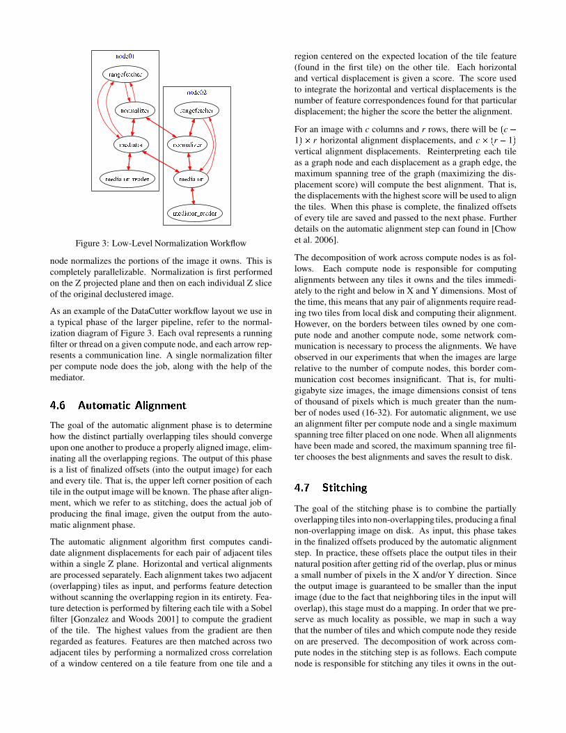
Figure 3: Low-Level Normalization Workflow

node normalizes the portions of the image it owns. This iscompletely parallelizable. Normalization is first performedon the Z projected plane and then on each individual Z sliceof the original declustered image.

As an example of the DataCutter workflow layout we use ina typical phase of the larger pipeline, refer to the normal-ization diagram of Figure 3. Each oval represents a runningfilter or thread on a given compute node, and each arrow rep-resents a communication line. A single normalization filterper compute node does the job, along with the help of themediator.

sPt�± ²������+������wz�³²�{­w}������|����The goal of the automatic alignment phase is to determinehow the distinct partially overlapping tiles should convergeupon one another to produce a properly aligned image, elim-inating all the overlapping regions. The output of this phaseis a list of finalized offsets (into the output image) for eachand every tile. That is, the upper left corner position of eachtile in the output image will be known. The phase after align-ment, which we refer to as stitching, does the actual job ofproducing the final image, given the output from the auto-matic alignment phase.

The automatic alignment algorithm first computes candi-date alignment displacements for each pair of adjacent tileswithin a single Z plane. Horizontal and vertical alignmentsare processed separately. Each alignment takes two adjacent(overlapping) tiles as input, and performs feature detectionwithout scanning the overlapping region in its entirety. Fea-ture detection is performed by filtering each tile with a Sobelfilter [Gonzalez and Woods 2001] to compute the gradientof the tile. The highest values from the gradient are thenregarded as features. Features are then matched across twoadjacent tiles by performing a normalized cross correlationof a window centered on a tile feature from one tile and a

region centered on the expected location of the tile feature(found in the first tile) on the other tile. Each horizontaland vertical displacement is given a score. The score usedto integrate the horizontal and vertical displacements is thenumber of feature correspondences found for that particulardisplacement; the higher the score the better the alignment.

For an image with c columns and r rows, there will be�c ´

1 ¡ H r horizontal alignment displacements, and c H � r ´ 1 ¡vertical alignment displacements. Reinterpreting each tileas a graph node and each displacement as a graph edge, themaximum spanning tree of the graph (maximizing the dis-placement score) will compute the best alignment. That is,the displacements with the highest score will be used to alignthe tiles. When this phase is complete, the finalized offsetsof every tile are saved and passed to the next phase. Furtherdetails on the automatic alignment step can found in [Chowet al. 2006].

The decomposition of work across compute nodes is as fol-lows. Each compute node is responsible for computingalignments between any tiles it owns and the tiles immedi-ately to the right and below in X and Y dimensions. Most ofthe time, this means that any pair of alignments require read-ing two tiles from local disk and computing their alignment.However, on the borders between tiles owned by one com-pute node and another compute node, some network com-munication is necessary to process the alignments. We haveobserved in our experiments that when the images are largerelative to the number of compute nodes, this border com-munication cost becomes insignificant. That is, for multi-gigabyte size images, the image dimensions consist of tensof thousand of pixels which is much greater than the num-ber of nodes used (16-32). For automatic alignment, we usean alignment filter per compute node and a single maximumspanning tree filter placed on one node. When all alignmentshave been made and scored, the maximum spanning tree fil-ter chooses the best alignments and saves the result to disk.

sPt�µ �+��w}����¶�wb���The goal of the stitching phase is to combine the partiallyoverlapping tiles into non-overlapping tiles, producing a finalnon-overlapping image on disk. As input, this phase takesin the finalized offsets produced by the automatic alignmentstep. In practice, these offsets place the output tiles in theirnatural position after getting rid of the overlap, plus or minusa small number of pixels in the X and/or Y direction. Sincethe output image is guaranteed to be smaller than the inputimage (due to the fact that neighboring tiles in the input willoverlap), this stage must do a mapping. In order that we pre-serve as much locality as possible, we map in such a waythat the number of tiles and which compute node they resideon are preserved. The decomposition of work across com-pute nodes in the stitching step is as follows. Each computenode is responsible for stitching any tiles it owns in the out-

put space. We make a one-to-one correspondence betweenownership regions in the input and output space. That is,if a compute node owned the first two rows of tiles in theinput space, it would own the first two rows of tiles in the(smaller) output space. In the majority of cases, the imagedata in the output space derives from image data in the inputspace on the same compute node. However, on the bordersbetween tiles owned by one compute node, and another com-pute node, some network communication will be necessaryto merge the final result. A single stitching filter per computenode executes this step.

sPt�· ¸¹�!�'º�wb���The goal of image warping [Wolberg 1994] is to geometri-cally transform an image; for our purposes, this means con-forming our stitched image (from the previous phase) to astandard appearance, i.e., to a pre-defined 2D atlas. Hav-ing standard image templates facilitates comparison betweenmultiple images of the same subject type. Image warpinginvolves the application of a mapping function that definesthe spatial correspondence between points in the input andoutput images. Examples of such functions include affine,bilinear or polynomial transformations [Wolberg 1994]. In2D, mapping functions f1 and f2 map a point

�x   y ¡ in one

image onto a point�u   v ¡ in the other image as follows:�

u   v ¢�» � f1�x   y ¡�  f2

�x   y ¡G¢ . In some warping algorithms, a for-

ward mapping function is defined and applied to each inputpixel to produce its output pixel location. In other warp-ing algorithms, an inverse mapping function is defined andapplied to each output pixel location to determine which in-put pixel to draw from to produce the output pixel. We em-ploy inverse mapping instead of forward mapping, becauseit ensures that all output pixels are computed, and prevents“holes” from occurring in the warped image.

It must be noted that we do not perform a 3D warp (warpingacross multiple Z planes), and that the 2D warping of each Zplane is independent of the other planes. Each Z plane is justa 2D image. So, view interpolation techniques like triangle-based warping[Fu et al. 1998] that help in visualizing depth-related information are not applicable in our case.

In our case, the user interactively defines a set of controlpoints over the image using a graphical interface called Jib-ber2, i.e. for each control point, the user identifies its positionin the input image, called “start” and its corresponding po-sition in the output image, called “end”. The start and endof each control point indicates the user’s requested change inthe image, that pixels at or near the start in the original imageshould move to a corresponding position at or near the endin the warped image. These control points as a set describehow the image should morph. Figure 4 shows how the con-trol points can be specified to warp an image of a portion ofthe brain so that it fits a standard brain atlas. On the left we

2http://ncmir.ucsd.edu/distr/Jibber/Jibber.html

see the unwarped image (colored region) overlay the atlas.On the right, we see the same image warped so as to fit theatlas dimensions. For a fairly large dynamic set of images,it may be possible to automate this initial step. For example,a feature extraction algorithm could probably find outlinesand void areas in the input image and match them againstthe contours from the output image (i.e. the atlas). Such anapproach may not scale well to very large images. So, as im-age size grows, we could use a low-resolution version of theimage in the automated control point generation process. Weused a manual approach because it is more general. Partialsections and sections of the image that are mangled in someway can still be registered with the atlas.

Given a set of control points, we generate approximate in-verse mapping functions to characterize the spatial corre-spondence and map the remaining points in the image. Thatis, given any pixel po’s location in the output space, we candetermine which candidate input pixel pi will contribute topixel po with minimum error. This is the first phase of in-verse warping, which we refer to as computation. In thesecond phase, which is called mapping, we assign the RGBcolor values at pi to po. Thus, the warping algorithm must it-erate over the output space and determine which areas of theinput space to read from. This correspondence is modeledusing low-order polynomials. We use the Weighted Least-Squares with Orthogonal Polynomials technique [Wolberg1994] to determine the inverse mapping transformation (ofsome order M) for each output pixel. This technique is verycompute intensive. Other faster techniques apply a singleglobal transformation to all pixels. However, this weightedtechnique takes pixel - control point locality information intoaccount to generate different transformations for each pixel,and thus provides better results3.

The computational workload is divided among the computenodes at the granularity of a tile. If a compute node owns agiven input tile ISx ¼ y ¼ z, then it will eventually own the outputtile OSx ¼ y ¼ z after the warp; that is, the tiling divisions do notchange, nor does the ownership of the corresponding tiles.Each node performs computation on the output tiles that itowns. In case the nodes are SMP machines, we have multiplefilters on these nodes, where each filter performs the warpingcomputation in parallel on different tiles. Thus, the initialdeclustering of the image dictates load balance.

The bigger challenge we face in warping is the mapping ofinput pixel RGB values to an output pixel in a distributed en-vironment. Here, an output pixel location within one tile mayhave its input pixel lie within the same or different (neighbor-ing or non-neighboring) tile. In either case, we need to readthe input tile to do the mapping. Reading input tiles on a per-pixel basis will be costly due to seek and network overheads.We do not know up front which input tiles will be needed

3We should note that our implementation is such that a user can easilyplug-in any warping technique to perform many kinds of warping transfor-mations.

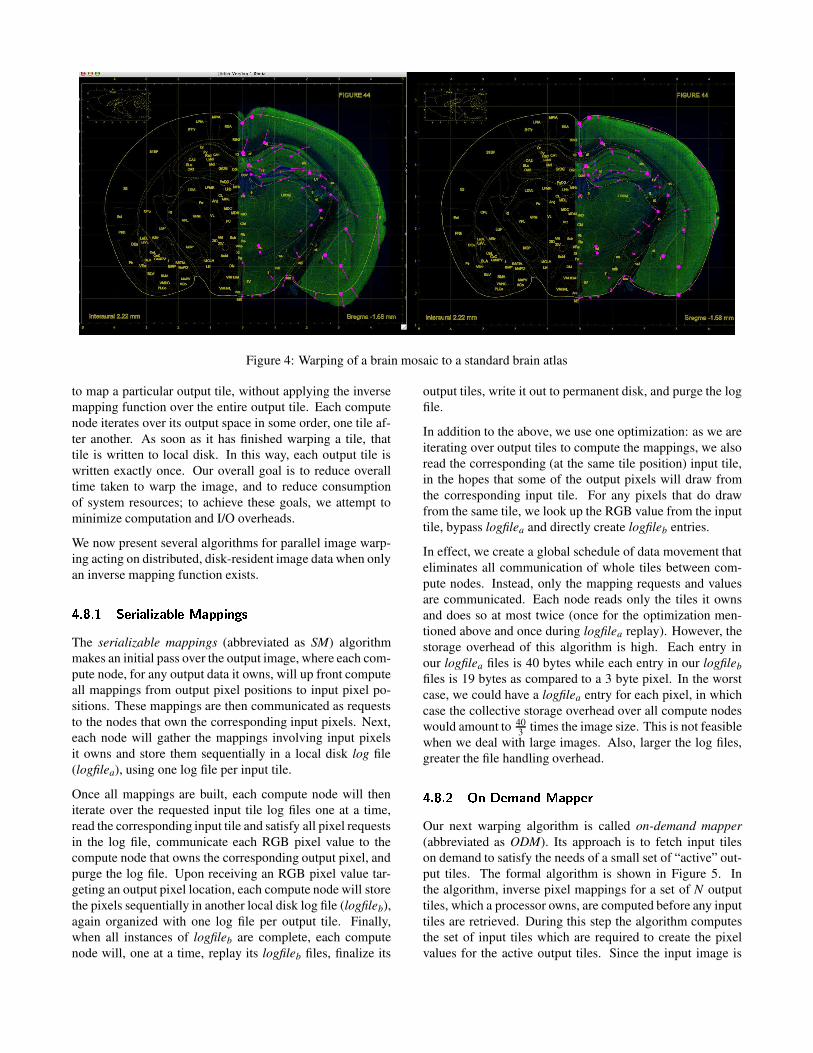
Figure 4: Warping of a brain mosaic to a standard brain atlas

to map a particular output tile, without applying the inversemapping function over the entire output tile. Each computenode iterates over its output space in some order, one tile af-ter another. As soon as it has finished warping a tile, thattile is written to local disk. In this way, each output tile iswritten exactly once. Our overall goal is to reduce overalltime taken to warp the image, and to reduce consumptionof system resources; to achieve these goals, we attempt tominimize computation and I/O overheads.

We now present several algorithms for parallel image warp-ing acting on distributed, disk-resident image data when onlyan inverse mapping function exists.

½F¾À¿�¾­Á Â�ÃÅÄ]ÆÈÇUÉÊÆÈËÌÇ«Í«É Ã�Î)Ç«ÏÐÏÐÆÀÑÓÒ«ÔThe serializable mappings (abbreviated as SM) algorithmmakes an initial pass over the output image, where each com-pute node, for any output data it owns, will up front computeall mappings from output pixel positions to input pixel po-sitions. These mappings are then communicated as requeststo the nodes that own the corresponding input pixels. Next,each node will gather the mappings involving input pixelsit owns and store them sequentially in a local disk log file(logfilea), using one log file per input tile.

Once all mappings are built, each compute node will theniterate over the requested input tile log files one at a time,read the corresponding input tile and satisfy all pixel requestsin the log file, communicate each RGB pixel value to thecompute node that owns the corresponding output pixel, andpurge the log file. Upon receiving an RGB pixel value tar-geting an output pixel location, each compute node will storethe pixels sequentially in another local disk log file (logfileb),again organized with one log file per output tile. Finally,when all instances of logfileb are complete, each computenode will, one at a time, replay its logfileb files, finalize its

output tiles, write it out to permanent disk, and purge the logfile.

In addition to the above, we use one optimization: as we areiterating over output tiles to compute the mappings, we alsoread the corresponding (at the same tile position) input tile,in the hopes that some of the output pixels will draw fromthe corresponding input tile. For any pixels that do drawfrom the same tile, we look up the RGB value from the inputtile, bypass logfilea and directly create logfileb entries.

In effect, we create a global schedule of data movement thateliminates all communication of whole tiles between com-pute nodes. Instead, only the mapping requests and valuesare communicated. Each node reads only the tiles it ownsand does so at most twice (once for the optimization men-tioned above and once during logfilea replay). However, thestorage overhead of this algorithm is high. Each entry inour logfilea files is 40 bytes while each entry in our logfilebfiles is 19 bytes as compared to a 3 byte pixel. In the worstcase, we could have a logfilea entry for each pixel, in whichcase the collective storage overhead over all compute nodeswould amount to 40

3 times the image size. This is not feasiblewhen we deal with large images. Also, larger the log files,greater the file handling overhead.

½F¾À¿�¾ÀÕ ÖWÑ�×cÃÓØ�ÇUÑ«Ù�Î)Ç«ÏÐϬÃÓÄOur next warping algorithm is called on-demand mapper(abbreviated as ODM). Its approach is to fetch input tileson demand to satisfy the needs of a small set of “active” out-put tiles. The formal algorithm is shown in Figure 5. Inthe algorithm, inverse pixel mappings for a set of N outputtiles, which a processor owns, are computed before any inputtiles are retrieved. During this step the algorithm computesthe set of input tiles which are required to create the pixelvalues for the active output tiles. Since the input image is

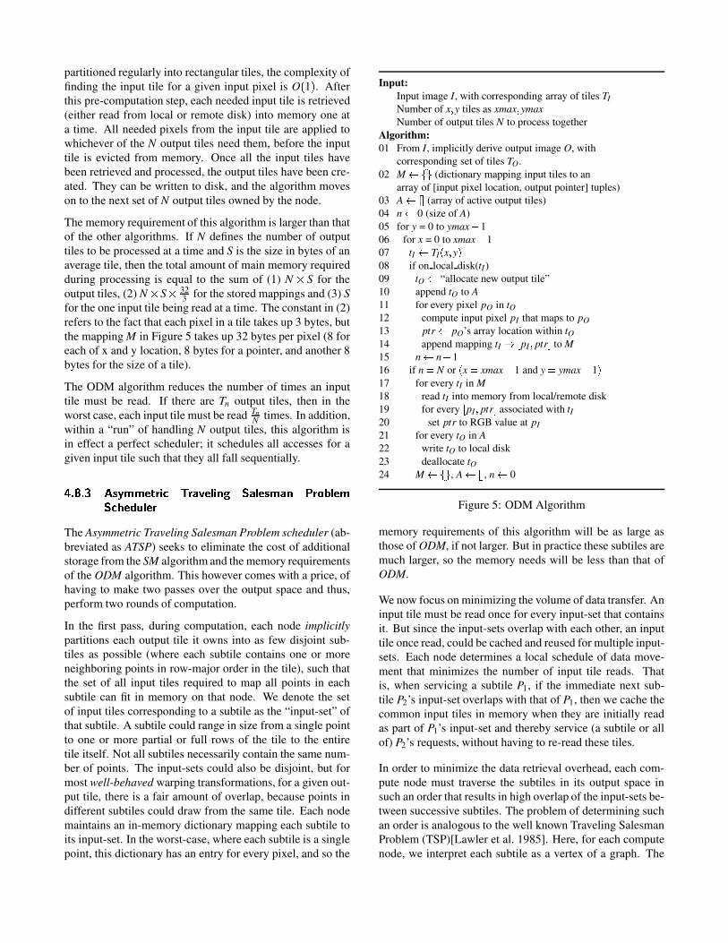
partitioned regularly into rectangular tiles, the complexity offinding the input tile for a given input pixel is O

�1 ¡ . After

this pre-computation step, each needed input tile is retrieved(either read from local or remote disk) into memory one ata time. All needed pixels from the input tile are applied towhichever of the N output tiles need them, before the inputtile is evicted from memory. Once all the input tiles havebeen retrieved and processed, the output tiles have been cre-ated. They can be written to disk, and the algorithm moveson to the next set of N output tiles owned by the node.

The memory requirement of this algorithm is larger than thatof the other algorithms. If N defines the number of outputtiles to be processed at a time and S is the size in bytes of anaverage tile, then the total amount of main memory requiredduring processing is equal to the sum of (1) N H S for theoutput tiles, (2) N H S H 32

3 for the stored mappings and (3) Sfor the one input tile being read at a time. The constant in (2)refers to the fact that each pixel in a tile takes up 3 bytes, butthe mapping M in Figure 5 takes up 32 bytes per pixel (8 foreach of x and y location, 8 bytes for a pointer, and another 8bytes for the size of a tile).

The ODM algorithm reduces the number of times an inputtile must be read. If there are Tn output tiles, then in theworst case, each input tile must be read Tn

N times. In addition,within a “run” of handling N output tiles, this algorithm isin effect a perfect scheduler; it schedules all accesses for agiven input tile such that they all fall sequentially.

½F¾À¿�¾ÀÚ ÛPÔ�ÜÓØ�ØCÃ�Ý>ÄÞÆÈßáà�Ä�ÇÅâiÃÅÉÊÆÀÑUÒ ÂFÇUÉ Ã�Ô#Ø�Ç«Ñ ã�Ä�ä�Í«É ÃUØÂFßiåUÃiÙ�æÐÉ ÃÅÄThe Asymmetric Traveling Salesman Problem scheduler (ab-breviated as ATSP) seeks to eliminate the cost of additionalstorage from the SM algorithm and the memory requirementsof the ODM algorithm. This however comes with a price, ofhaving to make two passes over the output space and thus,perform two rounds of computation.

In the first pass, during computation, each node implicitlypartitions each output tile it owns into as few disjoint sub-tiles as possible (where each subtile contains one or moreneighboring points in row-major order in the tile), such thatthe set of all input tiles required to map all points in eachsubtile can fit in memory on that node. We denote the setof input tiles corresponding to a subtile as the “input-set” ofthat subtile. A subtile could range in size from a single pointto one or more partial or full rows of the tile to the entiretile itself. Not all subtiles necessarily contain the same num-ber of points. The input-sets could also be disjoint, but formost well-behaved warping transformations, for a given out-put tile, there is a fair amount of overlap, because points indifferent subtiles could draw from the same tile. Each nodemaintains an in-memory dictionary mapping each subtile toits input-set. In the worst-case, where each subtile is a singlepoint, this dictionary has an entry for every pixel, and so the

Input:Input image I, with corresponding array of tiles TINumber of x ç y tiles as xmax ç ymaxNumber of output tiles N to process together

Algorithm:01 From I, implicitly derive output image O, with

corresponding set of tiles TO.02 M èêé'ë (dictionary mapping input tiles to an

array of [input pixel location, output pointer] tuples)03 A è�ì í (array of active output tiles)04 n è 0 (size of A)05 for y = 0 to ymax î 106 for x = 0 to xmax î 107 tI è TI ï x ç y ð08 if on local disk(tI )09 tO è “allocate new output tile”10 append tO to A11 for every pixel pO in tO12 compute input pixel pI that maps to pO13 ptr è pO’s array location within tO14 append mapping tI ñ ì pI ç ptr í to M15 n è n ò 116 if n ó N or ï x ó xmax î 1 and y ó ymax î 1 ð17 for every tI in M18 read tI into memory from local/remote disk19 for every ì pI ç ptr í associated with tI20 set ptr to RGB value at pI21 for every tO in A22 write tO to local disk23 deallocate tO24 M èxé'ë , A è�ì í , n è 0

Figure 5: ODM Algorithm

memory requirements of this algorithm will be as large asthose of ODM, if not larger. But in practice these subtiles aremuch larger, so the memory needs will be less than that ofODM.

We now focus on minimizing the volume of data transfer. Aninput tile must be read once for every input-set that containsit. But since the input-sets overlap with each other, an inputtile once read, could be cached and reused for multiple input-sets. Each node determines a local schedule of data move-ment that minimizes the number of input tile reads. Thatis, when servicing a subtile P1, if the immediate next sub-tile P2’s input-set overlaps with that of P1, then we cache thecommon input tiles in memory when they are initially readas part of P1’s input-set and thereby service (a subtile or allof) P2’s requests, without having to re-read these tiles.

In order to minimize the data retrieval overhead, each com-pute node must traverse the subtiles in its output space insuch an order that results in high overlap of the input-sets be-tween successive subtiles. The problem of determining suchan order is analogous to the well known Traveling SalesmanProblem (TSP)[Lawler et al. 1985]. Here, for each computenode, we interpret each subtile as a vertex of a graph. The

set difference between the input-sets of any two subtiles isthe weight of the edge between the corresponding vertices inthe graph. Hence, the cost of traveling from one vertex toanother is the amount of input tile data that needs to be readto service all requests in the destination’s input-set. Since setdifference is not always commutative, the resultant graph isasymmetric. So we have an instance of an asymmetric TSP(hence the name ATSP scheduler). Each compute node, thendetermines a least cost path that starts at any subtile and tra-verses every subtile exactly once 4. There are many heuris-tic algorithms to solve the ATSP. For our work, we use theeffective LKH [Helsgaun 2000] implementation of the Lin-Kernighan heuristic [Lin and Kernighan 1973]. We observedthat LKH, like other TSP-solvers, was rather slow for largegraphs. For a large number of subtiles, solving for the TSPwas contributing significantly to the overall warping time,thereby undoing the benefits of reducing the subtile reads.Thus, to handle a large number of subtiles effectively, webreak down the ATSP problem into smaller instances, whereeach instance handles all subtiles within a single output tile.The number of subtiles within each output tile tends to besmall when compared to the total number of subtiles. A com-pute node solves each instance, i.e. it determines the orderof traversal of the subtiles within each output tile it owns,such that the number of input tile reads for each output tileis minimized.

A disadvantage of the above approach is that we lose outon potential reuse of input tiles across different output tiles.So, as a current extension, we are trying to view our origi-nal problem as a hierarchical TSP: At the higher level, eachcompute node needs to determine an order of traversal ofoutput tiles, so that the overall number of input tile readsis minimized. One approach to solve this is to model it asa specific instance of the Generalized Traveling SalesmanProblem (GTSP) [Lawler et al. 1985]. The GTSP consists ofdetermining a least cost tour passing through each of severalclusters of vertices of a graph. Each output tile can be inter-preted as one such cluster and the subtiles within each tile asthe vertices within that cluster. Our notion of edge weight isthe same as before. Each compute node needs to determine aleast cost path that starts at any cluster, traverses every clus-ter exactly once and passes through exactly one vertex withineach cluster. To solve a GTSP, we need to transform it intoan instance of ATSP of equivalent or larger size[Ben-Ariehet al. 2003]. Here again, we expect the resulting problem tobe so large that LKH will consume a large amount of time.We are currently looking at different approaches to solve thisproblem. At the lower level, each node solves a small ATSPinstance within each output tile. This way, each node deter-mines an optimal path that covers the entire output space.

Once the least cost path for output space traversal is deter-mined, each node makes its second pass over the output tiles

4Actually, the problem is one of finding the shortest Hamiltonian path inan asymmetric graph, but this can easily be reduced to an instance of ATSP.

it owns; only, this time it services input tile requests in the or-der determined by the ATSP scheduler. For a subtile withinan output tile, we read its entire input-set at once (by defini-tion, this is guaranteed to fit in memory). We re-compute theinput pixel for each point within the subtile. This input pixelis already in memory, and so we assign its RGB color valuesto the output point. When this is repeated for every subtile,the entire output tile is finalized and can be written to localdisk.

ô õ÷öD\ N 7iEøp N5= 6�8WV `�N 4�BWV�6F4

Our experiments were carried out using a cluster of 32 com-pute nodes. The cluster, which was provided through an NSFResearch Infrastructure grant, consists of dual-processornodes equipped with 2.4 GHz AMD Opteron processorsand 8 GB of memory, interconnected by both an Infinibandand 1Gbps Ethernet network. The storage system consistsof 2x250GB SATA disks installed locally on each computenode, joined into a 437GB RAID0 volume with a RAIDblock size of 256KB. The maximum disk bandwidth avail-able per node is around 35 MB/sec for sequential reads and55 MB/sec for sequential writes.

For all of our experiments, we maintained more-or-lesssquare images to emulate what would be expected in real ap-plications. To scale up images for large-scale experiments,we would generate replicas of smaller images originatingfrom a confocal microscope, reproducing the tiles to theright, below, and the lower right. This enabled an easy scale-up by a factor of 4.

®�tGu ¨ ©j���«ª"|��¬��w­�+�úù ¯����#����{­w­°¬�l��w­�+�úù ²��lû������{­w}������|����«ùD����yü�+��w}����¶�wb���ý�+��|�º!�

In these experiments we evaluate the scalability and relativecost of each step of the image processing pipeline. In Fig-ure 6(a), we apply Z Projection, Normalization, Autoalign-ment and Stitching to a 6GB input image (49152x46080x1pixels), while varying the number of nodes from 1 to 16.This figure shows the relative performance of each stage. Weobserve that autoalignment is the most expensive in all cases.We also conclude that as the number of compute nodes aredoubled, the total runtime is roughly cut in half, thus almostlinear speedup is achieved in each of these steps.

The next set of experiments look at the performance of eachstep when the size of the dataset is scaled. In Figure 6(b), weapply the same processing steps, using 16 compute nodes,to a 1.5GB, 6GB, 25GB, 100GB and 400GB image. In eachstep, the image size is increased by a factor of 4, so we shouldexpect the runtime to increase by a factor of 4, if we arescaling linearly. Our results confirm linear scalability, sincethe total runtime increases by no more than a factor of 4 witheach dataset size increase.

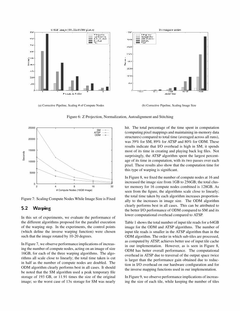
(a) Corrective Pipeline, Scaling # of Compute Nodes (b) Corrective Pipeline, Scaling Image Size

Figure 6: Z Projection, Normalization, Autoalignment and Stitching

0

5000

10000

15000

20000

25000

3216842

Sec

onds

# Compute Nodes (16GB Image)

SMATSPODM

Figure 7: Scaling Compute Nodes While Image Size is Fixed

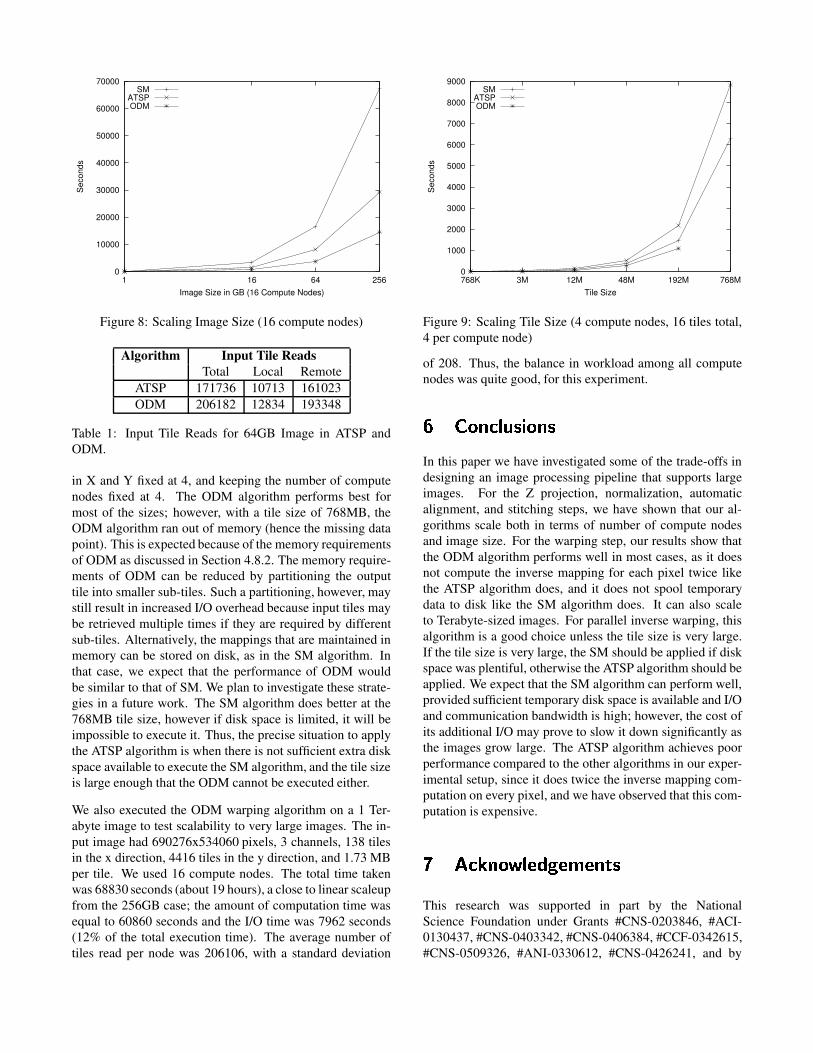
®�t�� ¸¹�!�'º�wb���In this set of experiments, we evaluate the performance ofthe different algorithms proposed for the parallel executionof the warping step. In the experiments, the control points(which define the inverse warping function) were chosensuch that the image rotated by 10-20 degrees.

In Figure 7, we observe performance implications of increas-ing the number of compute nodes, acting on an image of size16GB, for each of the three warping algorithms. The algo-rithms all scale close to linearly; the total time taken is cutin half as the number of compute nodes are doubled. TheODM algorithm clearly performs best in all cases. It shouldbe noted that the SM algorithm used a peak temporary filestorage of 193 GB, or 11.91 times the size of the originalimage; so the worst case of 13x storage for SM was nearly

hit. The total percentage of the time spent in computation(computing pixel mappings and maintaining in-memory datastructures) compared to total time (averaged across all runs),was 39% for SM, 89% for ATSP and 80% for ODM. Theseresults indicate that I/O overhead is high in SM; it spendsmost of its time in creating and playing back log files. Notsurprisingly, the ATSP algorithm spent the largest percent-age of its time in computation, with its two passes over eachpixel. These results also show that the computation time forthis type of warping is significant.

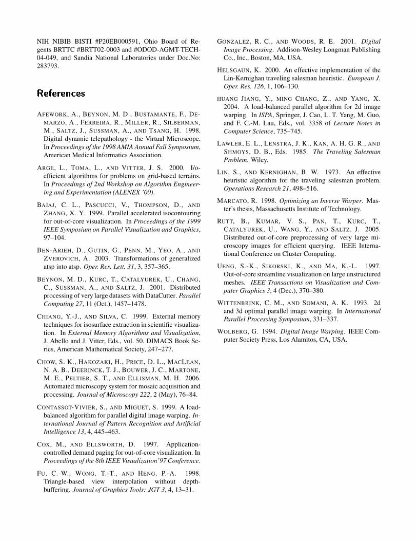
In Figure 8, we fixed the number of compute nodes at 16 andincreased the image size from 1GB to 256GB; the total clus-ter memory for 16 compute nodes combined is 128GB. Asseen from the figure, the algorithms scale close to linearly;the total time taken by each algorithm increases proportion-ally to the increases in image size. The ODM algorithmclearly performs best in all cases. This can be attributed tothe better I/O performance of ODM compared to SM and itslower computational overhead compared to ATSP.

Table 1 shows the total number of input tile reads for a 64GBimage for the ODM and ATSP algorithms. The number ofinput tile reads is smaller in the ATSP algorithm than in theODM algorithm. The order in which sub-tiles are processed,as computed by ATSP, achieves better use of input tile cachein our implementation. However, as is seen in Figure 8,ODM has better overall performance. The computationaloverhead in ATSP due to traversal of the output space twiceis larger than the performance gain obtained due to reduc-tion in I/O overhead on our hardware configuration and forthe inverse mapping functions used in our implementation.

In Figure 9, we observe performance implications of increas-ing the size of each tile, while keeping the number of tiles

0

10000

20000

30000

40000

50000

60000

70000

25664161

Sec

onds

Image Size in GB (16 Compute Nodes)

SMATSPODM

Figure 8: Scaling Image Size (16 compute nodes)

Algorithm Input Tile ReadsTotal Local Remote

ATSP 171736 10713 161023ODM 206182 12834 193348

Table 1: Input Tile Reads for 64GB Image in ATSP andODM.

in X and Y fixed at 4, and keeping the number of computenodes fixed at 4. The ODM algorithm performs best formost of the sizes; however, with a tile size of 768MB, theODM algorithm ran out of memory (hence the missing datapoint). This is expected because of the memory requirementsof ODM as discussed in Section 4.8.2. The memory require-ments of ODM can be reduced by partitioning the outputtile into smaller sub-tiles. Such a partitioning, however, maystill result in increased I/O overhead because input tiles maybe retrieved multiple times if they are required by differentsub-tiles. Alternatively, the mappings that are maintained inmemory can be stored on disk, as in the SM algorithm. Inthat case, we expect that the performance of ODM wouldbe similar to that of SM. We plan to investigate these strate-gies in a future work. The SM algorithm does better at the768MB tile size, however if disk space is limited, it will beimpossible to execute it. Thus, the precise situation to applythe ATSP algorithm is when there is not sufficient extra diskspace available to execute the SM algorithm, and the tile sizeis large enough that the ODM cannot be executed either.

We also executed the ODM warping algorithm on a 1 Ter-abyte image to test scalability to very large images. The in-put image had 690276x534060 pixels, 3 channels, 138 tilesin the x direction, 4416 tiles in the y direction, and 1.73 MBper tile. We used 16 compute nodes. The total time takenwas 68830 seconds (about 19 hours), a close to linear scaleupfrom the 256GB case; the amount of computation time wasequal to 60860 seconds and the I/O time was 7962 seconds(12% of the total execution time). The average number oftiles read per node was 206106, with a standard deviation

0

1000

2000

3000

4000

5000

6000

7000

8000

9000

768M192M48M12M3M768K

Sec

onds

Tile Size

SMATSPODM

Figure 9: Scaling Tile Size (4 compute nodes, 16 tiles total,4 per compute node)

of 208. Thus, the balance in workload among all computenodes was quite good, for this experiment.

þ S0? = 9PVÞB54lEG? = 4

In this paper we have investigated some of the trade-offs indesigning an image processing pipeline that supports largeimages. For the Z projection, normalization, automaticalignment, and stitching steps, we have shown that our al-gorithms scale both in terms of number of compute nodesand image size. For the warping step, our results show thatthe ODM algorithm performs well in most cases, as it doesnot compute the inverse mapping for each pixel twice likethe ATSP algorithm does, and it does not spool temporarydata to disk like the SM algorithm does. It can also scaleto Terabyte-sized images. For parallel inverse warping, thisalgorithm is a good choice unless the tile size is very large.If the tile size is very large, the SM should be applied if diskspace was plentiful, otherwise the ATSP algorithm should beapplied. We expect that the SM algorithm can perform well,provided sufficient temporary disk space is available and I/Oand communication bandwidth is high; however, the cost ofits additional I/O may prove to slow it down significantly asthe images grow large. The ATSP algorithm achieves poorperformance compared to the other algorithms in our exper-imental setup, since it does twice the inverse mapping com-putation on every pixel, and we have observed that this com-putation is expensive.

ÿ 1 9cZ = ? O V N @ mjN p N5= 6F4

This research was supported in part by the NationalScience Foundation under Grants #CNS-0203846, #ACI-0130437, #CNS-0403342, #CNS-0406384, #CCF-0342615,#CNS-0509326, #ANI-0330612, #CNS-0426241, and by

NIH NIBIB BISTI #P20EB000591, Ohio Board of Re-gents BRTTC #BRTT02-0003 and #ODOD-AGMT-TECH-04-049, and Sandia National Laboratories under Doc.No:283793.

`aN Q N 7 N5= 9 N 4

AFEWORK, A., BEYNON, M. D., BUSTAMANTE, F., DE-MARZO, A., FERREIRA, R., MILLER, R., SILBERMAN,M., SALTZ, J., SUSSMAN, A., AND TSANG, H. 1998.Digital dynamic telepathology - the Virtual Microscope.In Proceedings of the 1998 AMIA Annual Fall Symposium,American Medical Informatics Association.

ARGE, L., TOMA, L., AND VITTER, J. S. 2000. I/o-efficient algorithms for problems on grid-based terrains.In Proceedings of 2nd Workshop on Algorithm Engineer-ing and Experimentation (ALENEX ’00).

BAJAJ, C. L., PASCUCCI, V., THOMPSON, D., ANDZHANG, X. Y. 1999. Parallel accelerated isocontouringfor out-of-core visualization. In Proceedings of the 1999IEEE Symposium on Parallel Visualization and Graphics,97–104.

BEN-ARIEH, D., GUTIN, G., PENN, M., YEO, A., ANDZVEROVICH, A. 2003. Transformations of generalizedatsp into atsp. Oper. Res. Lett. 31, 3, 357–365.

BEYNON, M. D., KURC, T., CATALYUREK, U., CHANG,C., SUSSMAN, A., AND SALTZ, J. 2001. Distributedprocessing of very large datasets with DataCutter. ParallelComputing 27, 11 (Oct.), 1457–1478.

CHIANG, Y.-J., AND SILVA, C. 1999. External memorytechniques for isosurface extraction in scientific visualiza-tion. In External Memory Algorithms and Visualization,J. Abello and J. Vitter, Eds., vol. 50. DIMACS Book Se-ries, American Mathematical Society, 247–277.

CHOW, S. K., HAKOZAKI, H., PRICE, D. L., MACLEAN,N. A. B., DEERINCK, T. J., BOUWER, J. C., MARTONE,M. E., PELTIER, S. T., AND ELLISMAN, M. H. 2006.Automated microscopy system for mosaic acquisition andprocessing. Journal of Microscopy 222, 2 (May), 76–84.

CONTASSOT-VIVIER, S., AND MIGUET, S. 1999. A load-balanced algorithm for parallel digital image warping. In-ternational Journal of Pattern Recognition and ArtificialIntelligence 13, 4, 445–463.

COX, M., AND ELLSWORTH, D. 1997. Application-controlled demand paging for out-of-core visualization. InProceedings of the 8th IEEE Visualization’97 Conference.

FU, C.-W., WONG, T.-T., AND HENG, P.-A. 1998.Triangle-based view interpolation without depth-buffering. Journal of Graphics Tools: JGT 3, 4, 13–31.

GONZALEZ, R. C., AND WOODS, R. E. 2001. DigitalImage Processing. Addison-Wesley Longman PublishingCo., Inc., Boston, MA, USA.

HELSGAUN, K. 2000. An effective implementation of theLin-Kernighan traveling salesman heuristic. European J.Oper. Res. 126, 1, 106–130.

HUANG JIANG, Y., MING CHANG, Z., AND YANG, X.2004. A load-balanced parallel algorithm for 2d imagewarping. In ISPA, Springer, J. Cao, L. T. Yang, M. Guo,and F. C.-M. Lau, Eds., vol. 3358 of Lecture Notes inComputer Science, 735–745.

LAWLER, E. L., LENSTRA, J. K., KAN, A. H. G. R., ANDSHMOYS, D. B., Eds. 1985. The Traveling SalesmanProblem. Wiley.

LIN, S., AND KERNIGHAN, B. W. 1973. An effectiveheuristic algorithm for the traveling salesman problem.Operations Research 21, 498–516.

MARCATO, R. 1998. Optimizing an Inverse Warper. Mas-ter’s thesis, Massachusetts Institute of Technology.

RUTT, B., KUMAR, V. S., PAN, T., KURC, T.,CATALYUREK, U., WANG, Y., AND SALTZ, J. 2005.Distributed out-of-core preprocessing of very large mi-croscopy images for efficient querying. IEEE Interna-tional Conference on Cluster Computing.

UENG, S.-K., SIKORSKI, K., AND MA, K.-L. 1997.Out-of-core streamline visualization on large unstructuredmeshes. IEEE Transactions on Visualization and Com-puter Graphics 3, 4 (Dec.), 370–380.

WITTENBRINK, C. M., AND SOMANI, A. K. 1993. 2dand 3d optimal parallel image warping. In InternationalParallel Processing Symposium, 331–337.

WOLBERG, G. 1994. Digital Image Warping. IEEE Com-puter Society Press, Los Alamitos, CA, USA.