Retail Food Price Inflation Modelling

Project

Final Report

T.A. Lloyd, C.W. Morgan

(University of Nottingham)

J. Davidson, A. Halunga, S. McCorriston

(University of Exeter)

28th April 2011

Contents

Executive Summary 1

Aims of the Study 2

Section 1: UK Consumer Food Price Inflation 4

Section 2: The Drivers of UK Food Price Inflation 12

Section 3: Modelling UK Consumer Food Price Inflation 27

Section 4: Forecasting and Predictions 46

Section 5: Conclusions 51

Appendices

1. References

2. Listing of the Fitted Model

3. Within Sample Forecasts of Food Sub-group Models

4. Data definitions and sources

Executive Summary

Food price inflation peaked in the summer of 2008 at nearly 15%, a level not seen for

several decades. While the causes of this spike in food prices were of great interest, a more

pressing concern was to focus on the longer-term drivers of retail food prices, particularly

with regard to being able more readily to predict how they might develop in the future. The

focus on prediction lies at the heart of the project commissioned by DEFRA in the winter of

2009/10 and for which this report forms the outcome of the research undertaken.

Food price inflation has been rising at a time when world food and other commodity prices

- for example, wheat, oil and copper - have reached relatively high levels and it is possible

to draw a simple conclusion that domestic food price inflation simply reflects changing

world commodity market conditions. The report presented here demonstrates that while

there is some merit in this argument, it is in fact a much more complex process than this

line of argument suggests.

Empirical analysis based on modern econometric techniques shows that the major drivers

of the UK food price inflation, as measured by the CPI for food, are world commodity prices,

the Dollar-Sterling exchange rate, unemployment, labour costs and the price of oil. We find

that food price inflation is relatively unresponsive to changes in these drivers. The most

important determinant of food price inflation is world food prices with exchanges rates

also exerting a significant effect. We also find an important indirect role for oil through

world food commodity prices. These results imply that large changes in the values of these

drivers are required to affect domestic food price inflation. Results also suggest that shocks

that persist will tend to have a larger impact on food price inflation than one-off shocks

since the effect accumulates over time.

The estimated model forms the basis for a forecasting tool which not only provides an

opportunity to test different scenarios in a “What if...?” manner but also delivers monthly

forecasts of the level of food price inflation with appropriate bounds of confidence applied

in each case.

1

Aims of the Study

The boom in the prices of commodities in 2007 and 2008 led to a spike in inflation in many

economies across the globe that was quite sharp and somewhat unexpected. While the

response of the price of manufactured goods to rises in industrial commodity prices (for

example, oil) was significant, perhaps of more concern for all economies was the way

consumer food prices responded to sharp increases in soft commodity prices in a relatively

short period of time.

Although world commodity prices have subsequently fallen back, the emerging consensus

is that commodity prices will remain at higher levels relative to the past two decades and

be more volatile. The obvious concern that arises is the impact on households, particularly

in countries where expenditure on food accounts for a relatively high share of total

consumer expenditure. Even in countries where food expenditure accounts for a relatively

small share of the household expenditure, such as the UK, there are still important

distributional issues as the impact on the poorer sections of society can be considerable

even though the aggregate effect is small.

The recent developments in world commodity markets and the impact on consumer prices

have also raised concerns about future food security in many countries, including the UK.

Given the weight food products have in the calculation of consumer price inflation in many

countries, understanding the factors that caused this inflation is important but perhaps

more informative for policy makers is the ability to forecast any future rises with greater

accuracy and confidence.

The research project therefore has three main aims which are:

1. To review and evaluate existing understanding of UK consumer food price inflation

2. To model the drivers of UK consumer food price inflation

3. To create a tool that allow for forecasting and scenario setting to help policy makers

understand with greater certainty how UK consumer food price inflation might

develop in the future.

2

The research presented in this report outlines how these three aims were met. The work

was undertaken with a view to developing a forecasting tool that can allow policy makers

to undertake scenario setting exercises so that future patterns of food price inflation could

be understood with greater certainty than previously. As such, the report is structured as

follows. In Section 1, we review the history of consumer food price inflation in the UK and

make benchmark comparisons with other OECD countries. In Section 2, we provide the

background literature to the issue of food price inflation, covering the main causes of the

2007-2008 commodity price spike, the literature on price transmission and, more

generally, the links between commodity markets and inflation. This background serves as

the basis for selecting the appropriate econometric methodology which is outlined in

Section 3; this provides details on the rationale for the econometric methodology chosen,

the basis of the specific econometric model and results relating to the long-run relationship

between the main drivers of domestic retail food prices and, in particular, the links

between domestic food price inflation and world commodity markets. This econometric

model also serves as the basis for the forecasting tool, the interpretation of which is

provided in Section 4. Section 5 concludes,

In achieving these aims, the report begins by reviewing the evidence contained in food

price inflation data in the UK and then subsequently the views of the academic literature

that identify key drivers in food price inflation. Then drawing on this, data are collected

from publically available sources on a monthly basis to which modern time-series

econometric techniques are applied. The econometric analysis will focus on a number of

issues pertinent to food price inflation namely: magnitude and dynamic response to shocks

in the drivers of inflation and the extent of potential interaction between drivers. The

primary focus will be on aggregate food price inflation, as recorded in the Consumer Price

Index (CPI), with additional special analyses of specific food products. The outcomes from

the research will be the development of a clearer understanding of the factors that drive

food price inflation, quantification of the effects of the drivers and the dynamic response of

food price inflation to these drivers, understanding of price transmission mechanism in

specific food products and the creation of a tool to forecast food price inflation for

subsequent use by DEFRA.

3

Section 1: UK Consumer Food Price Inflation

The main measure used to calculate inflation in the UK is the Consumer Price Index (CPI),

which became the preferred measure in December 2003 replacing the Retail Price Index

(RPI). Both are still calculated although differences in the recorded values reflect the items

included in each index1; the major difference between the two is that the RPI includes the

costs of the housing market (mortgage interest for example) whereas the CPI does not. For

the purposes of this study we will be focussing mainly on the CPI and in particular the

component relating to Food and Non-Alcoholic Beverages. Divisions within the CPI are

given a weighting to reflect their importance within the consumer basket as shown in Table

1. The weights reflect spending in each specific year while the relative importance of food

in the overall CPI measure have increased in recent years as food prices have risen.

Table 1: Divisions and Weights within the CPI (Source: ONS, 2007)

Divisions Weight

01 Food and Non-Alcoholic Beverages 103

02 Alcoholic Beverages and Tobacco 43

03 Clothing and Footwear 62

04 Housing, Water, Electricity, Gas and other Fuels 115

05 Household Furnishings, Equipment and Maintenance 68

06 Health 24

07 Transport 152

08 Communications 24

09 Recreation and Culture 153

10 Education 18

11 Restaurants and Hotels 138

12 Miscellaneous Goods and Services 100

1 See ONS (2007). Another major difference is that CPI is calculated using a geometric mean of prices while RPI uses an arithmetic mean, the former potentially biasing the measure of inflation downwards in relation to the latter.

4

All the weights add to 1000 and the largest two categories are Recreation and Culture

(153) and Transport (152). The weight given to Food and Non-Alcoholic Beverages is just

over 10% of the total index (103) and is thus a key component of the measure of inflation

each month. All indices are calculated from samples of prices of goods and services and in

effect both indices (the RPI and the CPI) are “an average measure of change in the prices of

goods and services bought for the purpose of consumption by the vast majority of

households in the UK” (ONS, 2007).

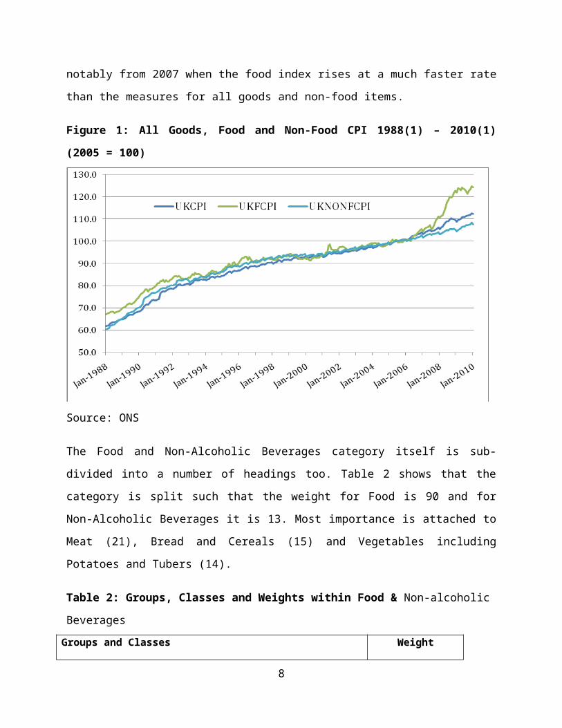
Figure 1 plots the index for all goods (UKCPI), the index for food (UKFCPI) and the index for

non-food items (UKNONFCPI), over a 22 year period. It is noticeable that while the trends

are similar there are divergences between the two, including most notably from 2007 when

the food index rises at a much faster rate than the measures for all goods and non-food

items.

Figure 1: All Goods, Food and Non-Food CPI 1988(1) – 2010(1) (2005 = 100)

Source: ONS

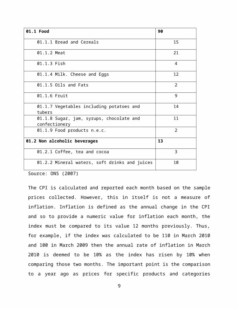
The Food and Non-Alcoholic Beverages category itself is sub-divided into a number of

headings too. Table 2 shows that the category is split such that the weight for Food is 90

5

and for Non-Alcoholic Beverages it is 13. Most importance is attached to Meat (21), Bread

and Cereals (15) and Vegetables including Potatoes and Tubers (14).

Table 2: Groups, Classes and Weights within Food & Non-alcoholic Beverages

Groups and Classes Weight

01.1 Food 90

01.1.1 Bread and Cereals 15

01.1.2 Meat 21

01.1.3 Fish 4

01.1.4 Milk. Cheese and Eggs 12

01.1.5 Oils and Fats 2

01.1.6 Fruit 9

01.1.7 Vegetables including potatoes and tubers 14

01.1.8 Sugar, jam, syrups, chocolate and confectionery 11

01.1.9 Food products n.e.c. 2

01.2 Non alcoholic beverages 13

01.2.1 Coffee, tea and cocoa 3

01.2.2 Mineral waters, soft drinks and juices 10

Source: ONS (2007)

The CPI is calculated and reported each month based on the sample prices collected.

However, this in itself is not a measure of inflation. Inflation is defined as the annual change

in the CPI and so to provide a numeric value for inflation each month, the index must be

compared to its value 12 months previously. Thus, for example, if the index was calculated

to be 110 in March 2010 and 100 in March 2009 then the annual rate of inflation in March

2010 is deemed to be 10% as the index has risen by 10% when comparing those two

months. The important point is the comparison to a year ago as prices for specific products

and categories might have fallen from one month to the next – suggesting deflation in the

6

mind of the consumer - but in relation to the same time one year ago, they could well have

risen and thus inflation is deemed to be rising.

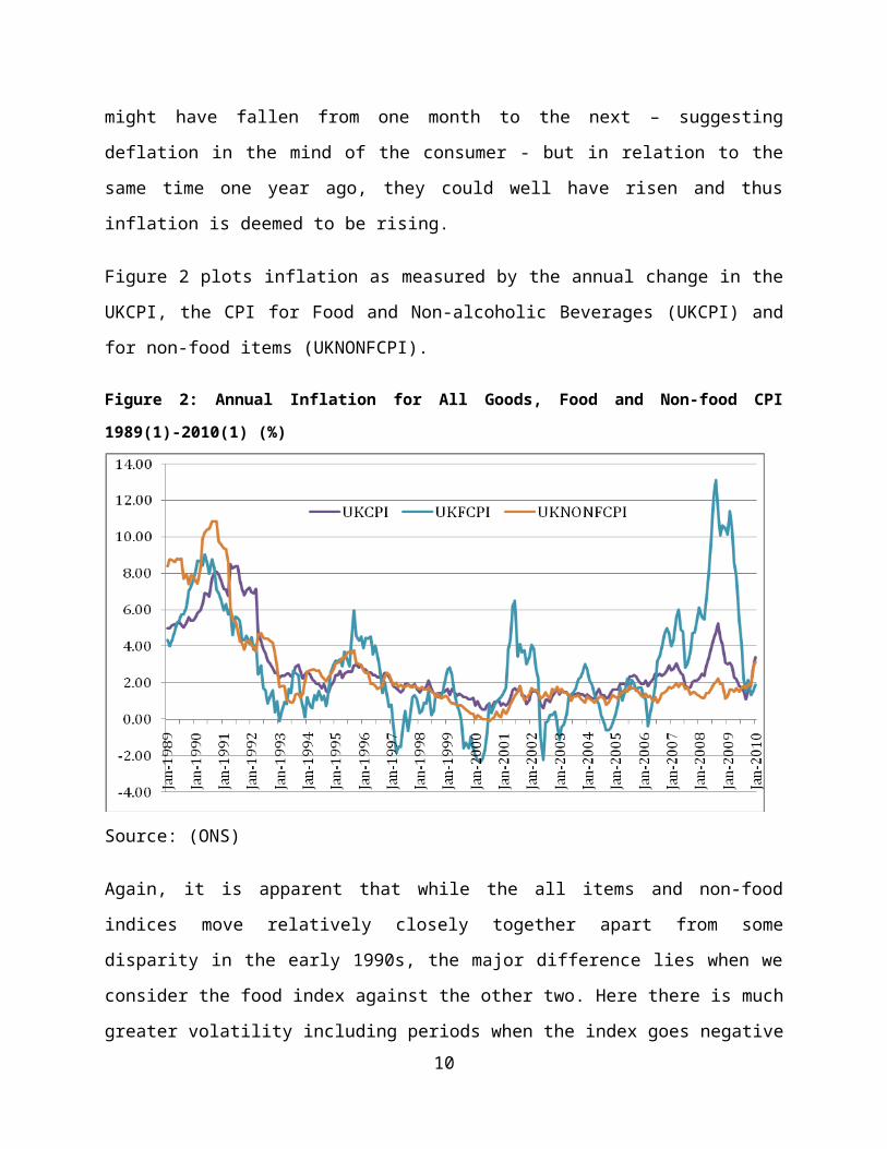
Figure 2 plots inflation as measured by the annual change in the UKCPI, the CPI for Food

and Non-alcoholic Beverages (UKCPI) and for non-food items (UKNONFCPI).

Figure 2: Annual Inflation for All Goods, Food and Non-food CPI 1989(1)-2010(1) (%)

Source: (ONS)

Again, it is apparent that while the all items and non-food indices move relatively closely

together apart from some disparity in the early 1990s, the major difference lies when we

consider the food index against the other two. Here there is much greater volatility

including periods when the index goes negative – i.e. the price of food items was actually

falling in nominal terms in 1997, 2000, 2002, 2005 and 2006. Equally, there are significant

peaks in food price inflation in July 1995 and mid-2001 as well as the outlier spike in prices

already mentioned in 2008. The evidence would suggest that food price inflation does

indeed behave differently to non-food price inflation and thus understanding the drivers of

food price inflation becomes a highly specific activity.

7

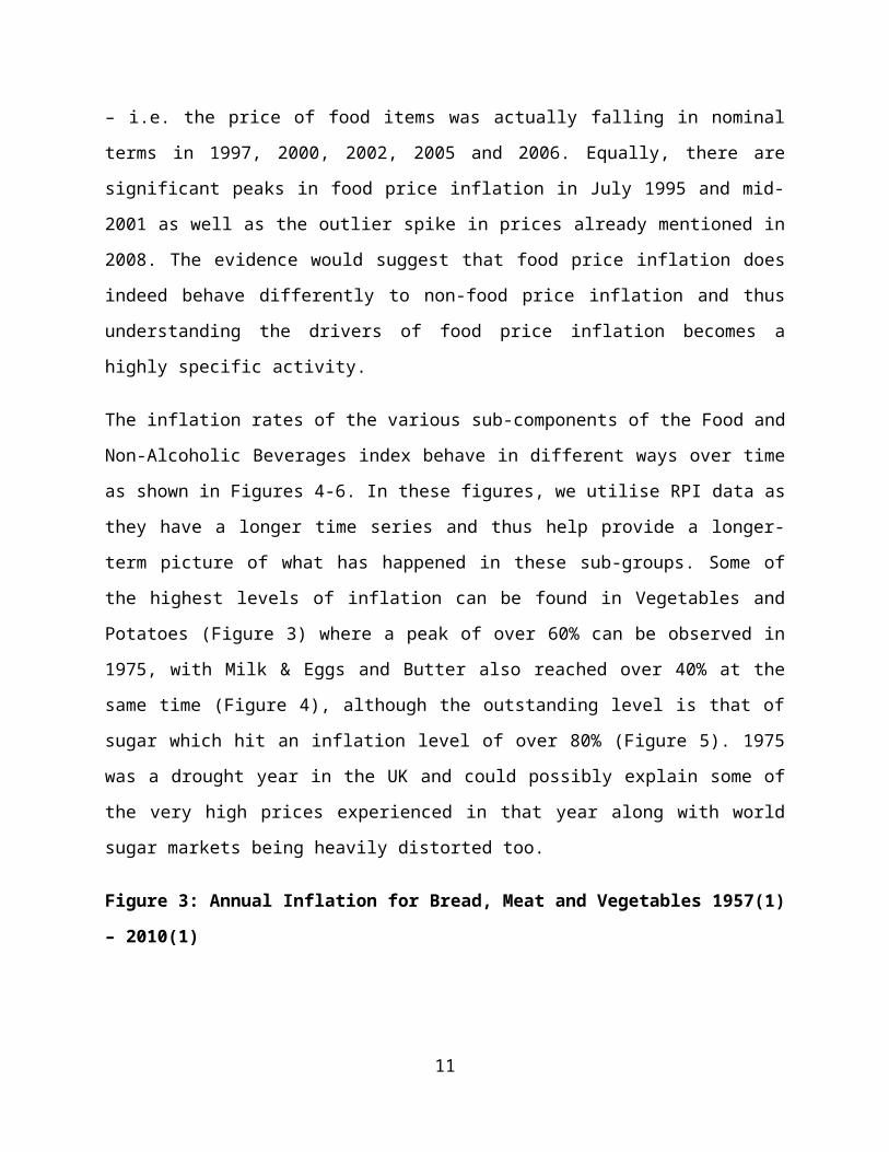
The inflation rates of the various sub-components of the Food and Non-Alcoholic Beverages

index behave in different ways over time as shown in Figures 4-6. In these figures, we

utilise RPI data as they have a longer time series and thus help provide a longer-term

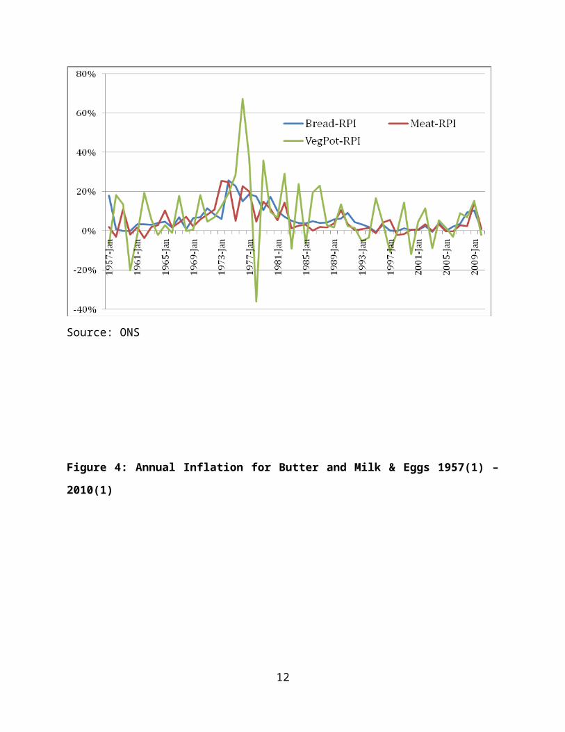
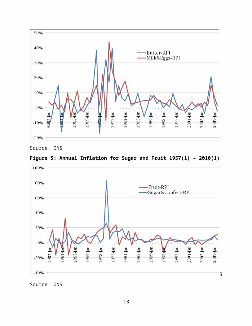
picture of what has happened in these sub-groups. Some of the highest levels of inflation

can be found in Vegetables and Potatoes (Figure 3) where a peak of over 60% can be

observed in 1975, with Milk & Eggs and Butter also reached over 40% at the same time

(Figure 4), although the outstanding level is that of sugar which hit an inflation level of over

80% (Figure 5). 1975 was a drought year in the UK and could possibly explain some of the

very high prices experienced in that year along with world sugar markets being heavily

distorted too.

Figure 3: Annual Inflation for Bread, Meat and Vegetables 1957(1) – 2010(1)

Source: ONS

8

Figure 4: Annual Inflation for Butter and Milk & Eggs 1957(1) – 2010(1)

Source: ONS

Figure 5: Annual Inflation for Sugar and Fruit 1957(1) – 2010(1)

S

Source: ONS

9

It is evident that patterns of food price inflation are very different across the sub-categories

of the food index. There are often periods of negative inflation – something rarely seen in

the headline all items inflation index although the RPI in 2009 did turn negative for several

months – and there is a degree of volatility that perhaps could reflect a range of supply and

demand factors that influence the prices consumers pay for their food at the retail level.

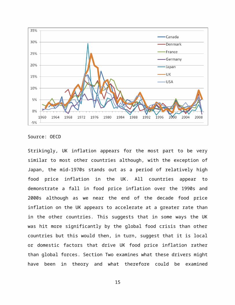
A key question follows from this analysis: how does UK food inflation compare with that in

other countries? Is the UK different or do food prices in fact follow a similar trend to other

countries? To that end, Figure 6 charts the CPI for food for a number of OECD countries,

some within the EU (Eurozone members and non-members) as well as outside the EU.

Figure 6: Food Price Inflation (CPI) of Selected OECD Countries 1960-2009

Source: OECD

Strikingly, UK inflation appears for the most part to be very similar to most other countries

although, with the exception of Japan, the mid-1970s stands out as a period of relatively

high food price inflation in the UK. All countries appear to demonstrate a fall in food price

inflation over the 1990s and 2000s although as we near the end of the decade food price

inflation on the UK appears to accelerate at a greater rate than in the other countries. This

10

suggests that in some ways the UK was hit more significantly by the global food crisis than

other countries but this would then, in turn, suggest that it is local or domestic factors that

drive UK food price inflation rather than global forces. Section Two examines what these

drivers might have been in theory and what therefore could be examined empirically to

understand the forces shaping UK food price inflation.

11

Section 2: The Drivers of UK Food Price Inflation

2.1 Introduction

A distinct and recently growing strand within the academic literature is one that focuses on

the movement in, and shocks to, global commodity prices and the subsequent impact on

domestic economies, an area that has seen renewed research effort following the

commodity price ‘spike’ of 2007/2008. While there are some parallels with the commodity

crisis of 1972-4 in terms of the underlying causes of the dramatic increases in world

commodity prices, there are also specific differences between the two ‘spike’ episodes.

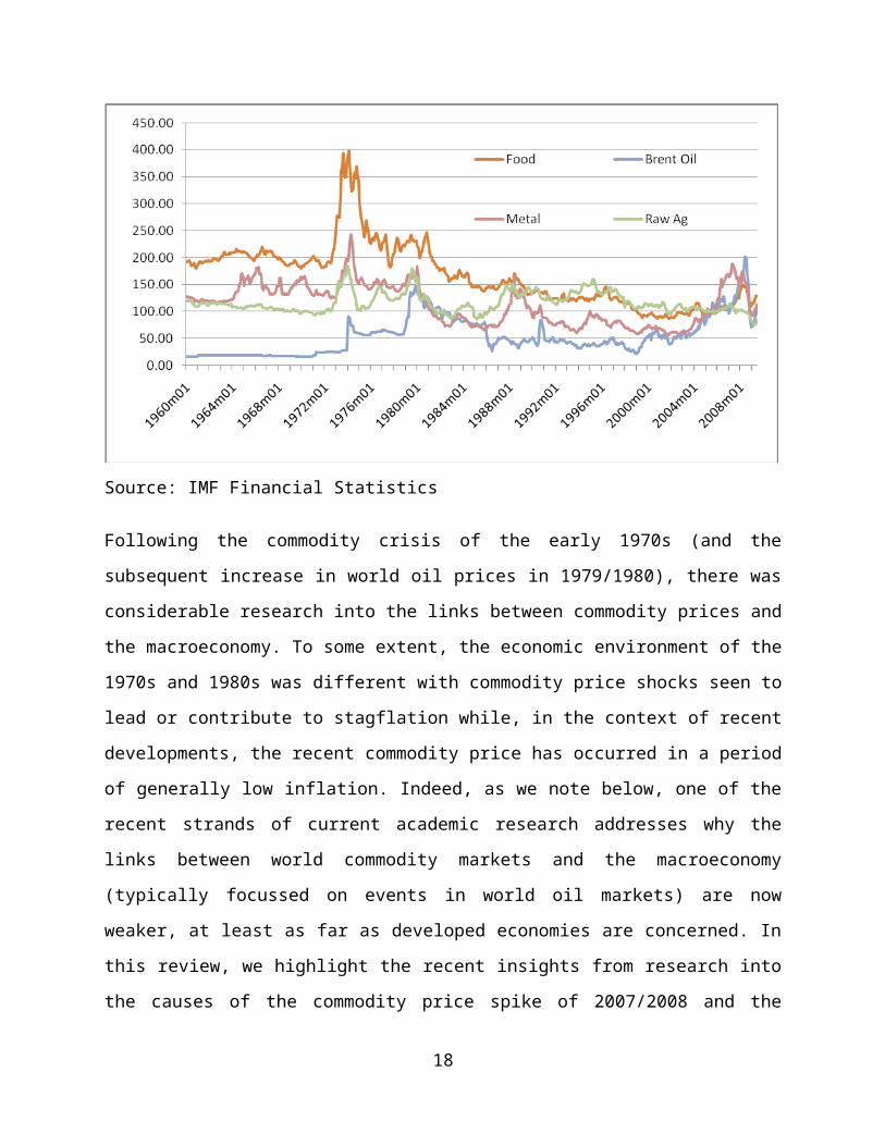
Figure 7 places recent developments in commodity markets in an historical context and

shows a series of world (non-oil) commodity prices and oil prices (both in real terms,

deflated by the US producer price index) from 1960 through to mid-2009. The figure shows

that, though the recent price spikes of 2007/2008 were substantive relative to the level of

real prices over the 1990s and 2000s, the spike was nevertheless much less significant than

the price changes that occurred in the early 1970s and, with respect to oil, the oil price

shock of 1979/1980.

Figure 7: World Real Prices (Monthly, 2005 = 100)

Source: IMF Financial Statistics

12

Following the commodity crisis of the early 1970s (and the subsequent increase in world

oil prices in 1979/1980), there was considerable research into the links between

commodity prices and the macroeconomy. To some extent, the economic environment of

the 1970s and 1980s was different with commodity price shocks seen to lead or contribute

to stagflation while, in the context of recent developments, the recent commodity price has

occurred in a period of generally low inflation. Indeed, as we note below, one of the recent

strands of current academic research addresses why the links between world commodity

markets and the macroeconomy (typically focussed on events in world oil markets) are

now weaker, at least as far as developed economies are concerned. In this review, we

highlight the recent insights from research into the causes of the commodity price spike of

2007/2008 and the potential impact this has on the macroeconomy and, in particular,

inflation. This will serve to inform the econometric strategy underlying the forecasting

model to address food price inflation in the UK. The review is divided into three parts. The

first focuses on the likely drivers of the 2007/2008 commodity price spike. The second

addresses the links between world commodity markets and how world prices are reflected

in domestic markets. The final part reports on recent research on the links between

commodity prices (principally oil) and inflation.

2.2 Drivers of Commodity Prices

Commodity price analysis often encompasses non-food items such as metals and energy as

well as the softer commodities such as for, example, wheat, sugar and coffee. While

recognising the vast literature in the general area of commodity markets – not least of

which is the seminal discussion on declining terms of trade for primary commodities (the

Prebisch-Singer hypothesis) - the focus here will be solely on soft commodity price analysis

which, in effect, can be thought of as raw food that is then processed to create food for sale

to final consumers. However, despite the narrow focus, it is clear from the wider

commodity literature that it is possible to observe inter-relationships between soft and

hard commodity price movements and in particular the key relationships between soft

commodity prices and energy (oil) prices. This will be returned to later in the review.

13

The literature on raw food commodity price analysis has seen a plethora of papers

published since the global food “crisis” of 2007/8 which replicated a similar pattern of

papers that grew from the oil and commodity price crisis of the mid-1970s (see, for

example, Hathaway, 1974). The implicit assumption in much of this recent research is that

there is a mapping from global raw food commodity prices into the food prices paid by

consumers for processed food, although this is not strongly articulated in most of the

papers. The exception to this is the way in which some poorer importing countries are

greatly affected by the transmission of global prices into domestic prices (particularly for

relatively unprocessed commodities such as rice) creating difficulties either for foreign

exchange reserves or indeed unrest due to food riots (see DEFRA (2008), Conceicao and

Mendoza (2009)).

Placing the recent food price spike in an historic context, Sumner (2009) along with OECD

(2008), suggest that earlier episodes had been more significant in terms of the scale of the

shock to food prices (e.g. the early 1970s) and the response to it in various economies, but

that these differences reflect the evolution in the macroeconomic environment at the time

when the shocks took place. The inference is that in a world where trade is freer, volumes

of trade are greater and macro environments are more flexible, the impact of a shock on a

given economy is perhaps less dramatic than when markets are more constrained,

macroeconomic policy is rigid and the extent of trade is limited. The role of economic

policy in harnessing inflationary expectations in face of macroeconomic shocks (e.g.

commodity price spikes) has been one of the recent insights from the macroeconomic

literature (see IMF, 2008).

Many of the recent papers take a descriptive view to explain the food price spike of 2008

(see, inter alia, OECD (2008), Trostle (2008), Mitchell (2008), Meyers and Meyer (2008)

and Sumner (2009)) mainly due to a need to provide some insights and perspectives to

what was a significant and potentially unique set of circumstances that created difficulties

for many countries particularly poorer ones (Wiggins and Levy, 2008). Given the need for

rapid explanation – policy makers were seeking solutions in the face of domestic unrest in

many countries such as Thailand, India and Haiti - there has been little scope to date for

14

more formal and considered econometric analysis that characterises papers relating to

commodity markets. Instead, simple statistical measures (correlations and covariances)

are typically presented as possible routes to identifying the major drivers for the food price

spike in 2008.

The impact of each potential driver has been debated and there are often interactions

between the key ones that become difficult to disentangle but ultimately, there is a strong

degree of consensus around which are the main factors causing the price spike; Sumner

(2009) provides a summary of the main drivers and, in essence, these can be categorised

into demand, supply and policy factors, with a further distinction arising in what are long-

term or trend effects and what are short-term or “spike” effects (Sarris (2008), Trostle

(2008)). Long-term effects include demand growth in emerging economies, the rising costs

of agricultural production, low stocks and the trade policy environment. Short-term or

spike effects include exchange rates, speculation, droughts and trade policy measures

designed to respond to the high prices.

Turning to the long-term factors first, it is apparent that global demand for commodities

has been growing steadily over the last thirty years but, in more recent times, has centred

on the rapid growth of emerging economies, especially China and India. Much of this

focuses on non-food commodities such as copper and oil but the impact is often felt in soft

commodity prices too through the oil price effects of transporting and producing

commodities along with dollar exchange rate effects (Piesse and Thirtle, 2009). However,

with economic growth comes increased wealth especially as labour moves from agrarian to

manufacturing work. The urbanisation of labour often leads to an increased demand for

calories and a change in the overall diet towards greater levels of processing and

convenience. Both can lead to increased demand in world markets for raw materials such

as wheat, soybeans and red meats. Indeed, some argue (e.g. Gilbert, 2010) that demand

factors are more helpful in explaining long term changes in commodity prices than supply

factors.

Increasing demand has also had an impact on the levels of stocks held internationally both

by governments and by private agents. While reliable and accurate measures of stocks are

15

always difficult to obtain, nevertheless some argue that the low levels of stockholding in

2006 onwards have been indicative of the tightness of world markets and are a

manifestation of both demand and supply factors (Piesse and Thirtle (2009), Wiggins and

Keats (2009)).

The supply of many of the major traded commodities, particularly wheat, has been affected

by unusual growing conditions in many of the major supplier nations but does not appear

to have arisen from falling agricultural productivity (Fuglie, 2008). However, the costs of

production for agricultural commodities have risen with rising oil and energy prices

meaning that the costs of production (e.g. fertilizer use) and the costs of transportation

have both risen significantly with a belief that this will continue in the longer term (Sarris,

2008).

Supply is also affected by a changing policy environment and this has also been blamed for

supply reduction in a number of areas. Mitchell (2008) argues that the policy-led moves in

the US and Europe towards greater use of biofuels produced from corn or sugar has

contributed around 65% of the food price spike through direct and indirect channels.

Improved incentives for farmers to switch from food to fuel production has led not only to

a reduction in the available food supplies of corn (maize) and some oil seed crops but also

to a reduction in soybeans in the US as the area normally planted to this crop has been

reduced due to the expansion of maize production.

The specific factors that appear to have been important in creating the spike – the short-

term effects – are varied but do not appear to have longevity in persisting in the long run. A

key factor in grain markets, for example, has been drought; Australia has had several years

of poor yields due to drought meaning that its contribution to world market supplies of

wheat has been severely diminished leading to upward pressure on prices. Equally,

recovery in yields in 2008/9 has eased world prices quite substantially, again highlighting

the sensitivity to specific shocks on the supply side.

16

Speculators have been viewed as a major force in driving up commodity prices rapidly and

without relation to fundamentals a view supported by some (Gilbert, 2010) although

others believe that speculators react to rather than create the higher prices (Irwin, 2009).

Another factor was the change in trade policy arising from government response to food

prices rising rapidly. There were many examples of countries taking exceptional measures

to protect domestic consumers at the expense of raising prices on world markets, a prime

case being that of Argentina where export taxes were levied on wheat to ensure sufficient

supplies remained in the country. Similar cases can be found in rice markets in south east

Asia where export bans were imposed in Thailand and Indonesia.

In drawing together the many and varied views on what drives soft commodity prices, it

would appear that the main long-term drivers have been global demand, the

macroeconomic environment (including exchange rate effects), agricultural production

tightness including low stock levels and the impact of oil. Specific short run factors such as

speculation, droughts and temporary trade policies can possibly help explain the short-run

spike witnessed in 2008 but are not important in the long-run.

World commodity prices have now fallen back from the peak of the 2007/2008 episode

though prices remain high-and are expected to remain so-relatively to the averages of the

1990s and 2000s (FAO, 2009). Although now lower, world commodity prices are

nevertheless expected to be more volatile thus underlying the importance of what drives

commodity prices both in the short and long-run and, in particular, how they are likely to

impact on the domestic economy, particularly domestic inflation. In the following sections,

we outline recent research that has been directed at addressing the links between world

and domestic prices and which will underpin the econometric model applied in this project.

2.3 Price Transmission

The previous section has reviewed the recent literature relating to the underlying

determinants of world market prices with particular reference to the commodity price

spike observed on world markets in 2007/2008. One notable feature of many of these

studies is that they refer to “food” price inflation while, in large part, what they are

17

essentially focussing on is raw commodity market prices which is fundamentally different

from the price of “food” that consumers typically purchase and consume, the raw

commodities to varying degrees undergoing significant amounts of processing before

reaching consumers. Moreover, the retail sector also adds a range of services, the cost of

which is bundled into the “food” product that consumers finally purchase. Therefore, in

addressing food price inflation at the consumer level as distinct changes in world market

“food” prices, economists and policy-makers need to address how world market prices are

transmitted through to retail prices. The literature that relates to these issues has two

important implications for this study of UK food price inflation: first, it highlights the other

factors that will have to be accounted for in determining food price inflation and, in turn,

the usefulness of the forecasting methods which subsequently follow; second, recent

developments in price transmission highlight the ‘right’ econometric approach to dealing

with these issues.

In focussing on the economic issues relating to the impact of world market prices on

domestic food prices, there are two aspects to price transmission that are important, The

first relates to the extent to which the change in world market prices are transmitted into

domestic market price for the same or similar commodity. For example, if the world market

price for wheat increases by 10 per cent, what is the commensurate change in domestic

wheat prices at the producer level? We can refer to this as “horizontal” transmission in that

it reflects a change in raw commodity prices on world markets into the change in the price

of the same commodity at a similar stage in the food chain. This topic relates to the ‘law of

one price’ and studies in this area address the extent to which markets are integrated; in

the context here, the extent to which domestic markets are integrated with world markets.

The second aspect relates to “vertical” price transmission which reflects how prices at one

stage in the food chain (say raw commodities) are transmitted into the change in the prices

of food (processed commodities) that consumers buy at the retail level.

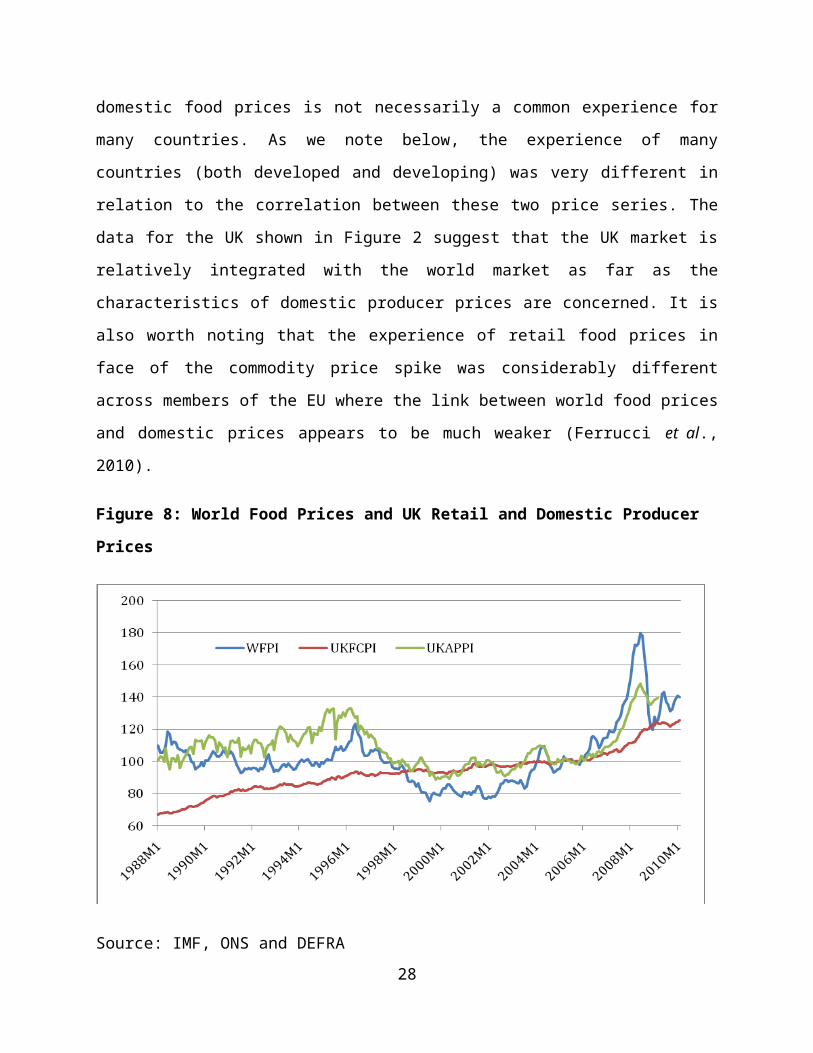
Figure 8 highlights the relevance of this distinction. The figure shows world commodity

prices (WFPI), UK producer prices (UKAPPI) and retail food prices (UKCPI) over the period

1988-2009. Eyeballing the data in Figure 8 suggests that the experience of each of these

18

prices series over this period was considerably different. World commodity prices relate

relatively closely (but not perfectly) to domestic producer prices, while the experience of

retail food prices is very different from the price changes occurring in world markets. It is

worth noting that the relatively close correlation between world market prices and

domestic food prices is not necessarily a common experience for many countries. As we

note below, the experience of many countries (both developed and developing) was very

different in relation to the correlation between these two price series. The data for the UK

shown in Figure 2 suggest that the UK market is relatively integrated with the world

market as far as the characteristics of domestic producer prices are concerned. It is also

worth noting that the experience of retail food prices in face of the commodity price spike

was considerably different across members of the EU where the link between world food

prices and domestic prices appears to be much weaker (Ferrucci et al., 2010).

Figure 8: World Food Prices and UK Retail and Domestic Producer Prices

Source: IMF, ONS and DEFRA

Retail food prices clearly behave differently from world market prices, the UK data for

retail prices over this period exhibiting less volatility compared with world market prices.

Clearly, if the concern is to forecast UK food price inflation, we have to address the link

19

between world market prices and retail food prices acknowledging that what happens in

world markets will have an impact on retail food prices but there are likely to be other

factors that cause retail prices to behave differently. In turn, there are some aspects related

to the theoretical aspects of price transmission that are going to be relevant in explaining

the different behaviour of the two price series. As noted above, the experience of the UK

may be different from that for other countries. Bukeviciute et al. (2009) document the

experience of food price transmission across EU member states following the 2007/2008

commodity price spike. While there can be many reasons why the experience should vary

so dramatically across “similar” countries, this is nevertheless an area which requires more

research. In broad terms, the likely candidates in explaining the varying experience across

the EU relate to the share of food expenditure in total consumer expenditure, the degree of

processing raw commodities undergo before reaching the retail level, the extent of

competition in the food processing and retail sectors and the role of government policies in

dampening the impact of world commodity price in the domestic market. Nevertheless, the

data reported in Figure 8 suggests that understanding the links between what happens in

world markets and how they are reflected in domestic retail food prices is important.

To reflect on these issues in greater depth, consider first of all the issue of “horizontal”

price transmission. Examples of empirical research relating to these aspects of price

transmission in agricultural markets include Ardeni (1989), Baffes (1991), Barrett (2001)

and FAO (2003). In terms of more recent events, there was a considerable amount of

observation around the time of the 2007/2008 world commodity price spike that the

domestic experience of prices for the same commodity across many countries varied

considerably. See, for example, FAO (2009) and the ‘Global Food Markets Group’ report

(HMG, 2009).

There can be many reasons why we would not expect complete “horizontal” price

transmission from world to domestic prices. For example, and most obviously,

governments have considerable flexibility over trade policy such as the lowering of tariff

barriers (or tariff-equivalent policies) can, in part, offset the rise in the purchase price of

commodities from world markets. This is most obviously true of commodity importing

20

countries but the role of government policies is also relevant for commodity exporting

countries, most notably Argentina which imposed export taxes on cereal exports during the

recent commodity price spikes. Governments may also have access to stocks which they

choose to deplete thus softening the rising costs of imports. In addition, governments may

also be willing to subsidise food during high price periods thus transferring the burden of

commodity price rises from consumers to the government exchequer. Finally, from a

macroeconomic perspective, the change in the exchange rate vis-à-vis the US dollar may

result in a lower or higher price increase in commodity prices when translated into

domestic currency terms. Figure 9 provides an indication of how the US dollar/sterling

exchange rate has moved over time.

Figure 9: US$:£ Exchange Rate 1988(1) – 2010(12)

Source: IMF Financial Statistics

The issue of “vertical” price transmission is an issue that has been subject to enquiry from

both an empirical and theoretical perspective. Early empirical work on this issue focussed

on single equation estimation with subsequent developments using more appropriate time

series techniques (specifically testing for co-integration and estimating error correction

21

models) to estimate the extent of pass-through from raw commodity prices to retail prices.

There are two related problems to these earlier studies. First, they often made little

reference to any theoretical model that may be consistent with the evidence of (typically)

incomplete pass-through that was found. Second, few studies paid any attention to other

factors that may determine retail food prices.

Theoretical models of vertical price transmission specify a framework where the

agricultural commodity passes into a downstream “food” sector that combines the raw

commodity with another input before being bought by retailers. With this simple structure,

there will be three factors which will be important in determining vertical price

transmission: the share of agricultural inputs in the “retail food” product purchased by

consumers; the nature of the technology of the food industry cost function which reflects

whether agricultural inputs can be substituted by other inputs if agricultural prices rise;

and finally the extent of competition in the downstream food sector. The most notable early

work on this issue was by Gardner (1975) who showed that, even with perfect competition,

the extent of price transmission will approximate to the share of the agricultural raw

product in the food industry cost function. So, if the share of the agricultural input was

25%, then for a given shock in the agricultural supply function, the price transmission

elasticity (reflecting the corresponding percentage change in retail prices relative to the

change in raw commodity prices) will be 25%. Imperfect price transmission can arise in

the Gardner framework depending on whether a variable proportions technology (rather

than a fixed proportions technology) is relevant. Wohlgenant (2001) provides a

comprehensive review of research that addresses the margins between the farm and retail

levels with considerable emphasis on models where the food industry is competitive.

McCorriston et al. (1998) take the Gardner model further by introducing imperfect

competition into the downstream food sector, an issue motivated by the increasing

concentration in the food sector (both at processing and retailing levels) in many

developed countries. They show that even relatively small degrees of imperfect

competition will dampen the price transmission effect such that the price transmission

effect will be less than 25% (as per the above example), the extent of price transmission

22

falling as the degree of imperfect competition rises. The reason for this is that while the

exogenous shock affects both agricultural and retail prices and the impact of this should

relate to the share of the raw commodity in the food industry cost function, with imperfect

competition, the mark-ups of the food industry adjust which, under relatively reasonable

conditions, offsets the role of the raw commodity share variable in determining the final

impact on the prices that reach consumers. Moreover, as we break down the number of

stages in the food chain into constituent parts (processing and retailing, say) with each of

these stages being imperfectly competitive, price transmission will decrease further. As

such, the a priori expectations from these theoretical models is that, with imperfect

competition in the food sector, retail food prices should not fully reflect changes observed

in world markets.

Most of the empirical work on vertical price transmission focuses on commodity/sector

specific studies. Examples include Lloyd et al. (2006) on the impact of food scares in the UK

and Sànjuan and Dawson (2003) who address the same topic, Kinnucan and Forker (1987)

for the US among others. Vavra and Goodwin (2005) provide a review of the recent studies

that address the issue of vertical price transmission from a number of perspectives and

over a broader range of case studies. However, given the nature of the techniques

employed, the time series models that have been applied cannot provide any information

on the factors that cause imperfect price transmission; so while the results of imperfect

price transmission are often consistent with the theoretical literature they do not, and

cannot given the nature of the techniques employed, pinpoint any particular factor (e.g.

imperfect competition in food industry) as the cause of the imperfect price transmission

effect.

Despite this, empirical modelling has progressed on issues that are less well dealt with in

the theoretical literature but consistent with causal observation about the behaviour of

food prices. As noted above, recent practice has used advanced econometric techniques

and, generally, reports imperfect price transmission. For example, recent econometric

methods can, or have the potential to, deal with issues such as asymmetric price

adjustment where the speed and size of price rises might not be the same as price falls (see

23

Meyer and von Cramon-Taubadel, 2004, for a review) and threshold adjustment which

addresses the issue that only significant price shocks are transmitted into retail prices and,

related, that price adjustment at different levels is non-linear. These relate to additional

issues that concern policy-makers. For example, a common concern often targeted as one

of the impacts of imperfect competition is that food processors and retailers are more

willing to pass on cost increases (or do so more quickly) but when it comes to cost

decreases, retail prices do not fall as much and/or do not fall as quickly. In relation to

threshold adjustment, these relate to the issue of non-linear price adjustment and would be

consistent with menu cost models in the macroeconomic literature (see Ball and Mankiw,

2004) whereby, due to the costs of changing prices on the supermarket shelf, retail prices

will not be changed if the price change of the commodity is small or is not expected to be

persistent. Alternatively, non-linear adjustment may relate to identifying substantive

commodity price shocks where the price shocks relate to some unexpected event which

may be based on the recent properties of commodity prices. For example, Hamilton (1996)

relates the oil price shocks to changes in oil prices over the previous 12 months on the

basis that price changes that reverse previous decreases will have little or no effect on

domestic variables.

One issue in future research will be to marry the casual observations regarding the

behaviour of prices together with econometric techniques that can explore these dynamics

in a more sophisticated manner and theoretical models (perhaps supported by structural

econometric models) that can better explain the retail food price behaviour that is

observed. Recent research on this issue is focussing on high frequency and highly dis-

aggregated data in order to give further insights into the behaviour of retail prices that

would not be obvious from relaying on aggregate data (see Nakamura and Steinsson,

2008). Finally, one further advantage in the application of these recent econometric

techniques over single equation models that ignore the fundamental issues associated with

the time series properties of the underlying data is that causality in terms of what price

drives the other does not have to be imposed but can be tested within the framework

applied. These issues are currently at the forefront of research in this area.

24

2.4 Commodity Prices and Inflation

Returning to the issue of horizontal and vertical price transmission and world commodity

prices and how this relates to the issue of inflation, there are two notable studies that deal

with these issues. First, the IMF noted that the transmission of world commodity price

shocks into core inflation was greater in emerging economies compared with the advanced

economies. Breaking down the analysis into two parts, they find that international to

domestic price transmission was less than domestic price transmission into core inflation.

In emerging economies, about one half of domestic price shocks are reflected in core

inflation, while for advanced economies, the corresponding estimate is less than one

quarter (IMF, 2008). Second, Ferruci et al. (2010) focus on food price pass-through in the

Euro area. They show that world commodity prices are a poor approximation for the cost

pressures faced by Euro-area food producers since the Common Agricultural Policy breaks

the link between what happens on world markets with what happens domestically. They

also show that dis-aggregation highlights many important differences between commodity

sectors. Apart from the dis-aggregation issue and the fact that they use a domestic

producer price index to highlight that world market prices are not necessarily the main

driver of what happens to domestic food prices, the study has the attraction that it employs

a vector auto-regression model and allows for non-linear adjustment. However, against

this, the authors do not allow for any other factors that may drive food prices, the

econometric model focussing solely on world to domestic producer prices and then

domestic producer to food prices, thus not specifying fully the drivers of domestic retail

food prices, an issue that we address in this report. Also, the model tackles the first

differences rather than the levels and thereby ignoring the possibility that the prices are

cointegrated which is key to forecasting accuracy.

Finally, given the focus of this report relates to the extent to which developments on world

commodity markets are reflected in domestic inflationary pressures, it is worth referring to

recent research on the links between oil price changes and inflation. There are several

papers that have addressed this link, most notably Blanchard and Gali (2007). In broad

terms, they address the issue relating to the relatively weak impact the recent oil price

25

spike on world markets had on inflation across a number of countries; in the context of the

terminology used above, the pass-through rate is now relatively low and has fallen over

time. This experience is in marked contrast to the experience of the 1970s and 1980s when

the oil price shocks were the main cause of stagflation in the 1970s and high inflation in the

1980s i.e. the pass-through rate was high. These studies show (Blanchard and Gali (2007)

for the US, Shioji and Uchino (2009) for Japan, De Gregorio et al. (2007) for a selection of

OECD countries) that the links between oil and the macro-economy are now considerably

weaker and this is true for a large number of countries.

There are several factors that could have given rise to this weaker link. These include:

reduced reliance on oil as opposed to other forms of energy such that oil now accounts for

a lower share of overall industry costs; differences in macro-economic policy whereby, in

recent years, governments have attained greater credibility of maintaining low inflation

such that inflationary expectations are not significantly altered in the face of unexpected

commodity price shocks; and more flexible labour markets. Blanchard and Gali (2007)

suggest all these factors have played a role in mitigating the impact oil price shocks have on

inflationary pressures. De Gregorio et al. (2007) however put more emphasis on the

declining share of oil in manufacturing costs. Covering both advanced and emerging

economies, the IMF (IMF, 2008) confirms the modest impact of oil price changes on

domestic prices and inflation; interestingly, their data indicates the impact of food prices

on inflation is potentially much greater in both advanced and emerging economies.

Finally, note that in the recent studies on the links between oil prices and inflation, a vector

autoregressive (VAR) model is typically employed. For example, the Blanchard and Gali

(2007) study of the oil price impact on inflation employ a four variable VAR model, this

specification being also the model applied in De Gregorio et al.’s (2007) extension of this to

a wider coverage of countries. As discussed elsewhere in the report, the VAR has a number

of advantages not least its incorporation of the long run for cointegration relationships in

the series, its emphasis of dynamics and that of not imposing causality on the

determination of what factors cause what in the empirical model. In line with this, the VAR

approach is also employed in this study.

26

Section 3: Modelling UK Consumer Food Price Inflation

The econometric modelling undertaken in this study has been developed to deliver

statistically reliable and economically interpretable information to inform policy makers

about the causes of UK food price inflation and the magnitudes and time lags involved.

Underlying the forecasts themselves is a modelling strategy that draws upon economic

theory, modern econometric methodology and specialist econometric software Time Series

Modelling4.31 developed by the teams’ principal econometrician, Professor Davidson. In

this section, we outline the principles of our modelling approach, how it relates to the

recent literature reviewed in the previous section and its distinctive features. The

modelling process is then summarised paying particular attention to the time series

properties of the data and how these are used in the estimation of the final model.

Interpretation of the econometric results and forecasts is presented in detail in the

following section.

3.1 Modelling Strategy: Four inter-related features

(i) Theoretical Underpinnings: Price Transmission

The model that has been developed for forecasting is built on the economic theory

underlying price transmission in food markets, whereby prices of raw food products are

transmitted in to retail food prices via the food service sector, which combines agricultural

output with the goods and services of food processing, manufacturing, distribution and

retailing to produce the food that consumers buy. As a result, the process begins with a

measure of raw commodity prices at both the domestic and world levels. Since World

commodity prices are expressed in US dollars, the $:£ exchange rate is required to convert

international price changes in to domestic prices. Finally, the price transmission model is

augmented with factors that may be expected to affect the consumer demand for food

(such as the rate of unemployment) and non-food supply factors which affect food industry

costs (such as labour costs and exchange rates). The basic structure of a price transmission

model is set out in Figure 10.

27

By basing the empirical model on the economics of price transmission, we can directly

incorporate economic theory into the process of model specification, greatly simplifying

the process of data collection and model search. Within this framework, the need to model

a potentially large set of factors that drive commodity prices is obviated, since their effects

are embodied in the world commodity prices themselves. The one exception to this in our

model is the inclusion of world oil prices. While this represents something of an

unnecessary complication for the purposes of forecasting price transmission, it allows the

effects of changes in oil prices on food inflation to be estimated directly. Price transmission

models also have the added advantage of being intuitive and their results easily

interpretable.

Figure 10: Price Transmission in the Food Chain

(ii) Econometric Techniques: Cointegration Analysis

As its name suggests, the price transmission model offers a theoretical framework for

determining the level of food prices rather than food price inflation (i.e. the rate of change of

food prices). This seemingly minor distinction plays a vital role in the econometric analysis

28

Demand (unemployment)

Supply (labour costs, exchange rate)

of time series data and arises because of the distinct statistical behaviour that characterize

the level and rate of change of most economic time series. As shown in the previous section,

the level of food prices (Figure 1) is characterised by a strong trend component, a feature

that is noticeably absent from the measure of the inflation variable itself, whether in its

period-on-period or annualised forms (Figure 2). In short, it is this distinction that the

techniques we adopt seek to exploit. To see why, notice that the trend in a time series, such

as the level of food prices, contains information regarding the behaviour of prices over the

longer term, information that would be lost if food price inflation, which is devoid of the

trend, were to be modelled directly. The upshot of this means that we can improve the

reliability and accuracy of forecasting food price inflation by utilizing the information

contained in the levels of food prices. To exploit this ‘long run information’ to help improve

short-term forecasting requires the application of a set of econometric techniques known

as cointegration analysis. In summary, by modelling the determinants of food prices rather

than food price inflation explicitly, our chosen approach allows the equilibrium

(cointegration) relationships involving food prices to be incorporated in modelling of food

price inflation, thereby improving forecast accuracy and reliability, particularly over longer

time horizons. While all forecasts and forecast methodologies are subject to unpredictable

factors that undermine their efficacy, particularly over long forecast horizons, the

discovery of cointegration and its incorporation in to empirical modelling has heralded

significant improvements in econometric modelling and forecasting performance.

Cointegration technology is at the heart of the forecasting model of food inflation

developed here.

(iii) Vector Autoregressive Methods: A Multi-Equation Model

While cointegration analysis may be undertaken in a single equation model, there are a

number of conceptual advantages in using a multi-equation framework, known formally as

a vector autoregressive (VAR) model. As discussed in the literature review, the VAR is the

most popular approach taken in the academic literature when undertaking analysis using

time series data. By incorporating the interdependencies between and the dynamics of the

29

variables of interest, the VAR offers a tractable tool for the estimation of the both the long

run (cointegrating) relationships and short-term forecasts.

(iv) Specialist Software: TSM version 4.31

The final distinctive element of our approach is the use of specialist econometric software

Time Series Modelling (version 4.31) developed by Professor Davidson. The software offers

a sophisticated analytical tool in which the stages of model specification, forecasting and

scenario analysis are integrated and unlike standard forecasting software, TSM generates

forecasts by the Monte Carlo method. This involves computing a dynamic simulation over a

number of steps by randomly re-sampling the measured shocks from the estimated system

thousands of times. This approach provides reliable forecast confidence intervals that do

not depend on supplementary assumptions such as normality. Plotting the quantiles of the

resulting distribution of simulations as ‘fan graphs’ provides a visual guide to the precision

of forecasts around their predicted values.

3.2 The Econometric Investigation

We now outline the data and methods adopted in development of the forecasting models.

Figure 11 summarises the process undertaken, which comprises four steps. Although

consideration of the forecasts and discussion of scenarios is an integral part of the

econometric investigation per se we discuss these in a separate results section that follows.

Data Collection

Using the theory of price transmission to identify the principal drivers of food price

inflation, the first step in the process is to collect appropriate time series data. In some

cases, there is little choice of which empirical measure to use (e.g. world food prices) or

indeed the choice was clear-cut as with the choice of exchange rate. However, for other

drivers (e.g. oil prices, exchange rates and manufacturing costs), several potentially

suitable variables are available. In selecting the final set of variables, factors such as sample

size, frequency and efficacy played important roles.

30

Figure 11: Steps in the Econometric Analysis

In searching for data for food manufacturing costs, it is apparent that no such data are

publically available and thus a proxy needs to be found. We considered two options: an

index of UK manufacturing costs (Figure 12) and an index of average earnings (Figure 13)

and found the latter performed best empirically (see below). Neither of these are obvious

measures of food industry costs; however, given the paucity of data in this respect we

opted for a measure that essentially captures labour costs, which for most elements of the

post-farm food chain is the major cost to be borne.

Turning to demand, ideally we would want to capture shifts in the demand curve for food

which at an aggregate level could include population changes (rejected as lacking

variability and also unavailable on a monthly basis), national income changes (again

rejected on similar grounds) or indeed prices of other goods (rejected due to the

endogenous relation between general inflation measures and food price inflation). Thus we

needed to have data on a monthly basis with appropriate variability that captured changes

in demand and as such we decided to utilise the monthly unemployment rate. As with our

proxy for industry costs this is not an obvious choice; however, it will reflect general

demand levels in the economy and has proven to work well empirically.

31

n

The outcome of this process determined the set of variables to be used in the econometric

modelling. 2 We adopt the convention of using the food CPI (Figure 1) as our principal

measure of food inflation. Meat, bread, fruit and vegetables sub-categories of the CPI are

used to measure inflation in these specific food groups (Figure 3).3 The world food price

index and the agricultural producer price index are used as the measures of international

and domestic food commodity prices respectively (Figure 8). To estimate the inflation

models for the four specific products - meat, bread fruit and vegetables – we use the UK

agricultural producer price indices (bread-making wheat, animals for slaughter (including

animal products), fresh fruit and vegetables respectively) alone and exclude international

prices on the grounds that international prices are likely to be of less importance for at

least some of these products. Oil prices are measured by the f.o.b. dollar price of Brent light

blend (Figure 14). Given that oil and world food prices are denominated in US dollars, we

also include the $:£ market exchange rate (see Figure 9).

Figure 12: Index of UK Manufacturing Costs 1988(1) – 2010(12) (2005 = 100)

Source: ONS

2 Definitions and sources of all data used in the analysis are detailed in Appendix 5.3 See ONS (2007)

32

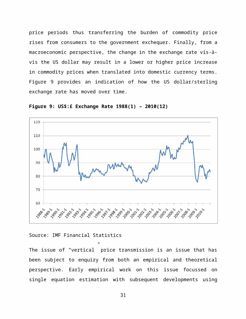
Figure 13: UK Average Earnings (seasonally adjusted) 1990(1) – 2010(12)

Source: ONS

Figure 14: Index of Dollar denominated Crude Oil Prices (Brent, light blend 38 API, fob U.K.) 1988(1) – 2010(12) (2005 = 100)

Source: IMF

33

The price transmission model is also augmented by supply and demand factors. On the

supply side, the index of average earnings is the preferred measure of labour costs and on

the demand side, the rate of UK unemployment (Figure 15). All series are available on a

monthly basis and have a 2005=100 base year. Data for the main food inflation model span

a twenty year sample, 1990(1) to 2010(12) giving 244 observations; those for the sub-

group models begin in 1996(1) since data on the subgroups are not available prior to this

date, and thus are based on samples containing 178 observations.

Preliminary Data Analysis

As previously mentioned the incorporation of the trend-like behaviour of variables forms a

central role in the modelling strategy, allowing models to incorporate information

pertinent to the long run when deriving short run forecasts. Cointegration analysis requires

that any variable that enters the equilibrium (or long run) relationship exhibits this

trending behaviour, known technically as a stochastic trend. Pre-testing each of the

variables confirms that all variables used in the analysis possess a stochastic trend and thus

can potentially play a role in both the long- and short-run parts of the model.

Figure 15: UK Unemployment Rate (%) 1988(1) – 2010(12)

Source: ONS

34

Model Estimation and Testing

The vector autoregressive (VAR) model of food prices contains seven equations, one

equation for each of the variables that form an econometric relationship with food prices,

so that there is an equation for world commodity prices, domestic producer prices, average

earnings, the unemployment rate, the $:£ exchange rate and oil prices. If necessary,

seasonal and other dummy variables also appear in the equations. This basic structure of

the VAR model is illustrated in Figure 16.

Figure 16: The variables determining food inflation in the VAR model

The modelling process adopts a ‘general-to-specific’ methodology whereby a wide range of

models are initially estimated and their forecast performance compared. Of fundamental

importance is the lag length of the VAR models, and this was found to be seven. Given that

the data are measured at a monthly frequency, this finding suggests that seven months of

the recent past are required to capture the relevant behaviour determining the level of UK

35

Seasonal and dummy variables

food prices. While models with longer lags also perform well, the large number of

statistically insignificant parameters they contain reduced estimation efficiency. As a key

objective of this study is to offer a guide to the reliability of the forecasts as well as

producing the forecasts themselves, the modelling attaches importance to the principle of

parsimony, whereby simpler models with shorter lags are preferred to more general

models containing redundant lags since, by doing so, confidence intervals around the

forecasts are reduced. To improve the efficiency of estimation and forecasting, redundant

variables have been removed in the final version of model so that all coefficients that

remain are statistically significant at conventional levels.4 Finally, the models that are

produced as a result of this process are also subjected to a battery of diagnostic checks for

model adequacy. These include tests of autocorrelation, heteroscedasticity, normality,

ARCH and functional form which, in general, passed at conventional levels of significance.5

Embedded in the basic structure of the estimated models are two cointegrating

relationships. The first represents the relationship between domestic food prices and its

determinants, namely world food commodity prices, the $:£ exchange rate, the rate of

unemployment and labour costs. As has been mentioned previously, the existence of an

equilibrium relationship involving food prices and the parameters that describe it are of

considerable conceptual and practical interest. Not only are the magnitudes of economic

significance in themselves (see the following sections) but the existence of an equilibrium

(cointegrating) relationship plays an important role in improving the reliability of forecasts

generated by the model. The second relationship represents the equilibrium between oil

prices and world food commodity prices. This is included to evaluate the effects of oil price

shocks on domestic food price inflation, a topic of significant policy interest.

While formal tests of the existence of cointegration have been applied to guide the

development of the final model, it is possible to give a flavour of the cointegration analysis

undertaken within the VAR with reference to Figure 17, which plots the log index of UK

food prices and the residuals from the two cointegrating relationship for which we find

4 The detailed specification of all final models is presented in the appendix.5 Diagnostic checking provided some evidence of non-linearity in some of the equations in the VAR. However, its precise form and extent could not be determined during a subsequent investigation, and thus we conclude that its effect is negligible.

36

evidence. Recall from the previous discussion of cointegration that it is the trending

behaviour of food prices - clearly visible from the plot - that contains the information

pertinent to the long term evolution of food prices; short-run behaviour describing

deviations around this trend. A set of variables that removes this trend can be treated as

explaining the long run behaviour of food prices and, in essence, this is what cointegration

analysis attempts to do: find a set of variables (and their regression parameters) that

remove the trend observed in the series of interest, in this case food prices. As is evident

from the two other series plotted in Figure 17 that represent deviations from their

respective equilibria - the so-called ‘cointegrating residuals’ - no trend remains.

Figure 17: Visualising Cointegration: Food Prices and the Cointegrating Residuals

from the Estimated VAR Model

1

2

3

4

5

6

7

8

9

10

50

60

70

80

90

100

110

120

130

140

logs

Inde

x 200

5=10

0

Index of Food Prices (left hand scale)

Residuals from the Food Price equilbrium (right hand scale)

Residuals from the Commodity Price - Oil Price equilbrium (right hand scale)

37

The importance of this finding lies in the fact that statistical methods can be used to

identify the economic causes of the long run behaviour of each of the equilibria i.e.

domestic retail food prices and world food commodity prices. Results also find that the

drivers to domestic retail food prices (i.e. world food prices, the $:£ exchange rate, the rate

of unemployment and labour costs) are found to be exogenous in the first equilibrium as is

oil prices to world food commodity prices in the second equilibrium. The implication of

these findings is that in the first equilibrium the causation is from the drivers to domestic

retail food prices and in the second equilibrium the causation is from oil prices to world

food commodity prices, as indeed economic intuition would suggest.

As alluded to above, in order to allow the effects of oil prices to be evaluated within the

VAR model, we specify a second cointegrating relationship between the index of world food

prices and the price of oil.6 Here too, oil was found to drive the long run behaviour of world

food prices than be driven by it, as would be expected if its principal role was to drive food

production costs through fuel and fertilizers.

The same methods have also been applied to the four sub-groups of food (bread, meat, fruit

and vegetables), with the exception that domestic producer prices alone are used owing to

the weaker links between the domestic and world market for these products. 7 In this

regard, it is also worth re-calling the recent work by Ferrucci et al. (2010) who also

emphasise the relevance of domestic producer prices rather than world market prices as

the main driver of domestic retail prices. Results from the sub-group models are broadly

similar and in most cases are superior to the overall model, a feature that most likely

reflects not only the product specificity but also the proximity of UK markets between

producer and retailer levels.

This section has outlined the data series used and the methods applied in the development

of the forecasting models for food prices and the four sub-groups. In summary, each

forecasting model is a seven equation Vector Autoregressive (VAR) model that satisfies

6 Residuals from this relation are similarly free of the strong trend that characterise the world food price index. Formal tests for cointegration are less clear-cut; however, we maintain the second cointegration relationship owing to the importance of oil in policy analysis. 7 Since these models did not contain international prices we do not include the second cointegration relation involving oil.

38

conventional diagnostic checks for model adequacy and exhibits the property of

cointegration. Key results and forecasts from these models are presented below.

3.3 Results

Long-Run Elasticities

As a prelude to the forecasting and scenario analysis, Table 3 reports long run elasticities of

UK food prices and food sub-groups with respect to the drivers.8 In the table, the figures

show the long-run or eventual effect of a 10% permanent increase in each driver on food

prices, keeping other factors held fixed. When interpreting the coefficients, it is important

to bear in mind the ceteris paribus (other factors held fixed) nature of these estimates.

Specifically, they provide estimates of the effect of a given 10% shock keeping the other

variables held constant. They do not estimate the effect of what would be observed

following a 10% shock, which necessarily reflect the net effect of the initial shock and all

the knock-on and feedback effects from the other variables in the system. We provide

estimates of these net long run effects in the following section using impulse response

analysis. Here, we report the traditional ceteris paribus elasticities. We will focus initially

on the elasticities of the Food CPI, commenting on the elasticities from the sub-groups later

on.

Results indicate that the response of retail food prices to changes in each of the drivers is

inelastic, in that a 10% shock to each driver leads to a less than 10% effect on retail food

prices. The largest elasticities are found to be with respect to world food commodity prices

and the $:£ exchange rate. As predicted by price transmission theory, world food

commodity prices are positively related to retail prices. Other drivers held fixed, a 10%

increase in agricultural prices on the world market is associated with a 6.33% increase in

food prices at the retail level. Price transmission is thus not one-for-one, reflecting the

8 Since the international markets for the sub-group products are less well defined, the drivers in price transmission are more principally domestic in nature, hence oil and world prices do not appear in these models. Note also that the oil price elasticity in the food model is mediated through commodity prices in the second cointegrating vector that is detected in the food model.

39

Table 3: The Long Run Effect of a 10% Change in the Drivers on the Prices of Food

and Food Sub-Groups

Food Bread Meat Fruit Vegetables

World food prices 6.33% --- --- --- ---

Domestic Farmgate Price

___ 3.31% 3.77% 2.51% 4.65%

Oil Prices 3.50% --- --- ---- ---

Exchange rate -5.09% -2.33% -1.00% -3.56% -4.19%

Labour costs 2.32% 5.25% 2.88% 4.44% 3.08%

Unemployment rate -1.59% --- --- --- ---

greater the volatility of world commodity markets compared to UK retail prices, as indeed

was highlighted in Section 1. The effect of oil price shocks is similarly muted in that a 10%

shock to the world price of oil, translates in to a 3.50% increase in retail food prices, other

factors held constant.

Recall that in addition to the international forces we have augmented the price

transmission model to allow for domestic supply and demand factors to impact on food

prices. We measure the non-food costs of producing food (food manufacturing costs) with

average earnings and these are also positively related to food prices, the long run effect of a

10% increase in labour costs leading to a 2.32% increase in retail food prices. We measure

shocks to domestic food demand with the rate of unemployment. As expected, the estimate

is negative and implies that, other factors held constant, a 10% increase in the rate of

unemployment leads to a 1.59% decrease in food prices.9

Results for the subgroup models yield broadly similar results in that price transmission

elasticities are positive and inelastic. Lying between 2 and 5%, they are a little lower than

the 6.3% obtained for food as a whole implying that retail prices of these products are

9 Note that like the other coefficients this is an elasticity and not a semi-elasticity so that it estimates the effect of a proportional (10%) change in the unemployment rate and not a 10 point change.

40

more stable, relative to farm-gate prices than for food as a whole. Since the farm-gate

prices are already priced in Sterling, the exchange rate merely reflects the effect of

overseas demand for these products and production costs. Our demand proxy, the rate of

unemployment did not have any discernible effect on the prices of the food sub-groups. It

should be noted that the sub-group models are estimated over a shorter sample period and

as such when aggregating the results from these sub-models we do not get equivalence

with the overall food price model results.

In summary, we find that all the elasticities are signed in accordance with intuition and are

inelastic in magnitude implying that food prices are relatively more stable than the drivers

that determine food prices.

The Effect of Shocks on Food Price Inflation

The long-run elasticities presented above indicate the responsiveness of food prices to each

of the drivers, keeping all other drivers held fixed (i.e. ceteris paribus). They are analogous

to the effects that might be observed if one were able to quantify the effect of the drivers in

some sort of controlled experiment. Useful though this is, where there are interactions

among the drivers (as is likely to be case between oil prices and the exchange rate for

instance) estimates predicated on the ceteris paribus assumption offer only a partial picture

of the likely impact of changes in the drivers.

Impulse response analysis provides a more complete picture of the effect of changes to the

drivers by relaxing the ceteris paribus assumption, and by doing so incorporates the knock-

on and feedback effects (so-called, second round effects) into the overall estimate of the

effect of changes to the drivers. For example, the effect of an exchange rate shock may

affect food prices inflation directly (via changing the relative price of imported and

exported food products) and indirectly (via its effects on oil prices). Impulse response

analysis delivers estimates of the net effect of the shock and, in this sense, it is more akin to

a ‘what if’ type of experiment, since it captures the model’s best estimate of what might

actually be observed following the shock.

41

Impulse response analysis also allows the effect of shocks of different durations to be

simulated, such as a one-off shock and a permanent shock. In the former, the shock is a one

period blip after which the driver reverts to its original level; in the latter the shock lasts

forever and thus the driver is shifted to a new level permanently. In either case, the

impulse response function shows the form and speed of the adjustment path over time

following the shock.

We present the impulse response analysis in Figures 18 and 19 to show the effect of a 10%

shock to each driver on the annualised rate of food price inflation. Each impulse response

function measures a separate experiment but are plotted together merely for convenience.

Each plots the predicted difference in the annualised rate of food inflation between the

‘with’ and ‘without’ shock scenarios. Since it is the effect on the annualised rate of inflation

that is measured on the vertical axis, the units of measurement are percentage points. The

impulse response functions in Figure 18 describe the effect on the annualised rate of food

inflation of a temporary (one-period) 10% shock in each driver for the 12 months following

the shock. 10

As can be seen, shocks to world food commodity prices and exchange rates have the largest

quantitative impact on the annualised rate of food price inflation. Furthermore, the effect is

typically largest in the month following the shock with subsequent impacts diminishing in

magnitude. For example, a one-off 10% increase in world food commodity prices is

estimated to increase the annualised rate of food inflation by almost 0.3 percentage points

(from say 3.0% to 3.3%) in the month immediately following the shock, whereas ten

months after the shock food inflation is only 0.1 percentage points higher. Lags of this sort

imply that the shocks to UK food inflation are immediate and continue to have an effect

over several months before food price inflation returns to equilibrium, supporting recent

evidence from other European countries.11 Turning to the effect of transitory exchange rate

10 The effect of larger shocks can be inferred simply by multiplying up the effect by the appropriate scalar. For example, the effect of a doubling in the level of the driver (i.e. a 100% shock) on the annualised rate of food inflation can be inferred by multiplying the impulse response functions by ten.

11 Modelling the persistence of shocks in the euro area Ferrucci, Jiménez-Rodríguez and Onorante (2010) find statistically significant effects up to 10 months after the shock.

42

Figure 18: Impact of a One-period 10% Shock to each Driver on Annualised Food

Price Inflation.

-0.3

-0.2

-0.1

0

0.1

0.2

0.3

0.4

1 2 3 4 5 6 7 8 9 10 11 12

Perc

ent

World Commodity Prices $ Oil Prices $:£ Exchange Rate Labour Costs Unemployment Rate

Months following shock

shocks, Figure 18 shows that if the $:£ exchange rate were to increase (i.e. the pound

depreciates against the $) by 10% for one month, the model predicts that annualised food

inflation would be around 0.23 percentage points lower in the following month and 0.1

percentage points lower 11 months later. The effect of oil prices is the exception to this

general pattern, suggesting that blips in oil prices have a more gradual effect in the months

following a shock, although as is evident from Figure 18, shocks of this magnitude have

only a very small impact on annualised food inflation. In all cases, the effect of these

temporary shocks eventually disappears as the shock becomes more distant.

In Figure 19, we simulate the effect of a permanent 10% increase in period 1 in each of the

drivers on the annualised rate of food inflation. In each simulation, the shock shifts the

driver in to a level that is permanently 10% higher, and as a result the effect on annualised

food inflation is far larger than in the temporary shock, building up over time and

persisting for longer. The peak impact occurs 12 months after the shock in all cases except

43

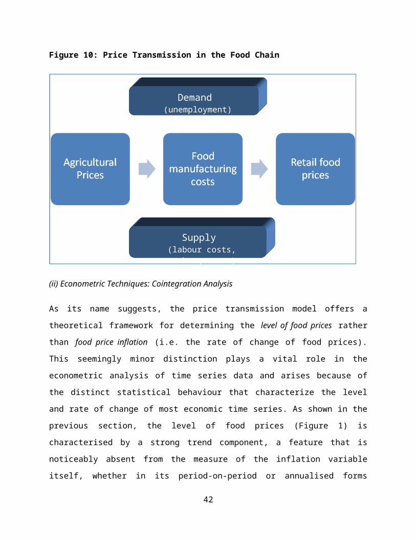
for oil price shocks, which again has a more gradual impact. As before, shocks to world food

commodity prices and exchange rates that have the greatest impact on food inflation. The

model predicts that were world commodity prices to rise 10% and remain there, food

inflation would initially increase by 0.3 percentage points (replicating the result of a

temporary shock) and steadily rise throughout the following year, peaking just under 2

percentage points higher some 12 months after the shock. With world food prices keeping

at their new higher level, food inflation remains higher for around a further year. A

permanent shift in the exchange rate induces a similar pattern albeit in mirror image, with

food inflation bottoming-out at around 1.8 percentage points lower 12 months following

the shock. Although these effects persist for a number of years, they do eventually vanish.

Figure 19: Impact of Permanent 10% Shock to Drivers on Annualised Food Price

Inflation.

-2.00

-1.50

-1.00

-0.50

0.00

0.50

1.00

1.50

2.00

1 2 3 4 5 6 7 8 9 10 11 12 13 14 15 16 17 18 19 20 21 22 23 24Perc

ent

World Food Commodity Prices $ Oil Prices $:£ Exchange Rate Labour Costs Unemployment Rate

Months following the s hock

44

The role of oil price shocks is perhaps more indirect than the other drivers. As we pointed

out earlier there is a direct relationship between oil and world food commodity prices with

the effect that oil prices feed into domestic food price inflation indirectly and more slowly.

This imperfect transmission is then further exacerbated by the fact that changes in world

food commodity prices are not fully transmitted to UK food retail price inflation. The effect

of oil is observed more clearly in the longer run as shown in Figure 19.

By simulating one-period and permanent shocks of this sort we are of course considering

polar scenarios, and intermediate cases, such as a 10% shock of 3 month duration, are

straightforward to calculate. However, by illustrating these extreme cases, it is possible to

offer an assessment of the lower and upper bounds of the likely effect of shocks of this

magnitude, with the effects of permanent shocks representing something of a worst case

scenario. For example, given that a 10% world food commodity price shock increases food

inflation by at most 2 percentage points, a 50% shock would at most increase food inflation

by 10 percentage points, with the peak impact being up to 12 months following the shock.

These findings underscore the simple but fundamental point that the longer the shock

persists the greater is the likely impact on food inflation.

45

Section 4: Forecasting and Predictions

The econometric methodology outlined in the previous section and the identification of the

main drivers of UK food prices forms the basis for the forecasting tool, the provision of

which is the primary aim of this project. Since the tool itself can be used to generate current

forecasts of food price inflation on demand, there seems little point presenting such

forecasts here. Rather, in this section of the report, we take the opportunity to present an

assessment of the model’s performance and undertake some scenario analysis. The latter is

not intended to be exhaustive but illustrates the sort of analysis that can be conducted

using the forecasting tool.

Forecast performance

In terms of overall forecasting performance, the principal way to gauge this is to estimate

the model over a shorter data period and forecast forward but within the sample period.

The forecasting ability of the model relates then to the forecasted values compared with

the actual data values as observed; the closer the prediction of the model to what was

observed, the better the forecasting performance of the model. In terms of the annualised

rate of food price inflation in the UK, the forecasting performance of the model is

highlighted in Figure 20.12 For the purposes of this exercise, the model has been estimated

over a sample that ranges from September 1990 to December 2009 and forecasted out to

December 2010. Hence it represents the forecasts that would have obtained had the model

been used to forecast food inflation in 2010, the green line represents the median predicted

forecast. To assess the performance of the model, we compare the forecasts for 2010 with

the actual inflation rate over the period. In presenting the figure, we have made use of a fan

chart (derived by Monte Carlo simulations) which represents confidence intervals within

which the predictions would be expected to lie. For example, the two outer extremes of the

fan chart represent the 99% confidence interval for the forecast, but clearly if the red actual

line was at the outer extremes of the fan chart, the lower is the accuracy of the forecasts.

12 Forecasts from the food subgroup models are presented in Appendix 4.

46

Inspection of Figure 20 suggests that the estimated model forecasts well, particularly over

short horizons, although, the more distant the forecasting period, the less precise the

forecasts become. Having forecasted food inflation well for the first four months, the model

over-predicts food inflation for most of the remainder of the period as errors in earlier

forecasts are incorporated into forecasts further out in time.

Figure 20: In-Sample Forecasting Performance of the Underlying Econometric Model.

Nevertheless, given the monthly frequency of the model this 12 month ahead forecast is

something of a long range forecast and, taken as a whole, the forecasting performance of

the model seems acceptable, the estimated model forms a strong basis for forecasting

future domestic food price inflation. It is also noteworthy that despite not hitting actual

inflation a year out, the model has predicted correctly a downturn and subsequent final

upturn, albeit as at a higher level that actually occurred.

Of course, an alternative way to address forecasting issues with the econometric model is

with reference to the fan diagrams. In essence, these avoid putting precise numbers on the

forecasts, allowing the forecaster to assess the outcomes of alternative scenarios with

47

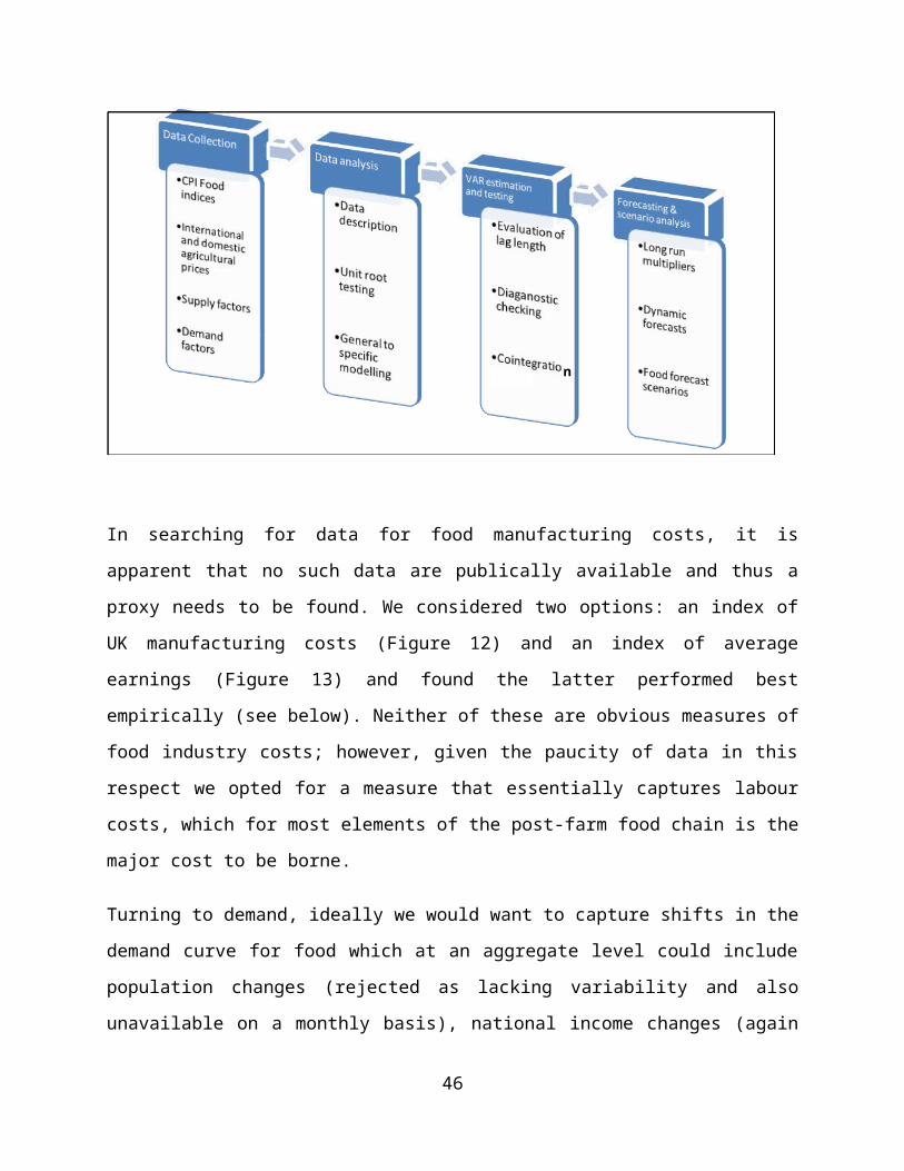
reference to intervals so that the forecaster can choose which portion of the fan chart the

results can be presented in – for example 20% or 40% around the median forecast value.

Notice that in the simulation in Figure 20, actual inflation has a tendency to lie towards the

extremities of the confidence interval for much of the forecast horizon.

Scenario Analysis

In addition to the generation of forecasts themselves, the model can also be used to

produce forecasts of UK food inflation arising from scenarios the forecast-user considers

important and interesting. This is carried out by changing a driver of domestic food prices

by a given percentage and using the model to forecast the expected impact on the

annualised rate of domestic food price inflation over a given period. While the effect of

temporary or permanent shocks can be simulated, for the purposes of this exercise we will

consider relatively large permanent shocks to world food commodity prices and the

exchange rate. Given the permanent nature of the simulated shock, the predicted response

will be something of a ‘worst case scenario’ to each of these large although plausible

shocks, since by their very nature, shocks tend to be short-lived. With these caveats in

mind, consider Figure 21 and Figure 22 which simulate what would have happened during

the 12 months of 2010 if there had been a permanent 50% increase in world food

commodity prices (Figure 21) and a 20% depreciation in the $:£ exchange rate (Figure 22)

in January 2010. For comparison, we also present the actual rate of food price inflation up

to August 2010 (the last available observation in our sample) alongside the simulations. As

can be seen from the figures, the introduction of our hypothetical shocks in January 2010

occurs during the period of food price inflation stability that had existed since the autumn

of 2009 however the tail of 2008/9 spike in food inflation is clearly visible and a useful

reference point. In January 2010, food inflation stood at 1.89%.

Referring to Figure 21 the introduction of a 50% shock to world food commodity prices in

January 2010 has only a modest effect on the rate of food inflation initially. However, by

May 2010, four months after the hypothetical shock, predicted food inflation rises to 5%

and within nine months the effect of persistently high commodity prices imparts a strong

48

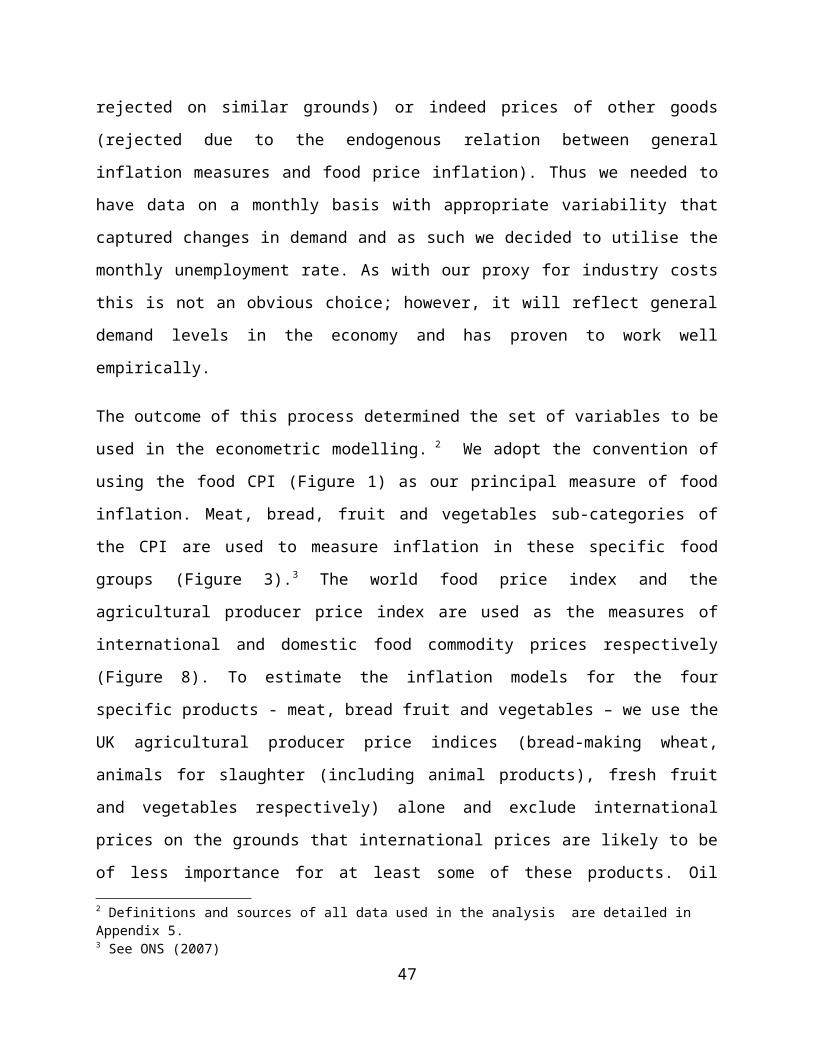
effect on domestic food inflation, which rises to around 11%, and subsequently peaks at

12% one year after the shock.

Figure 21: Simulated Food Price Inflation following a 50% Permanent shock to

World Food Prices in January 2010

The response of food price inflation to a 20% permanent exchange rate shock is shown in

Figure 22. As above, the immediate impact on food price inflation is similarly muted with

simulated inflation barely deviating from its actual path in the first three months after the

shock. The effect grows through the period with food inflation peaking at just over 6% in

September 2010.

Similar forecasts following the introduction of hypothetical shocks to the other drivers can

also be computed, although given that their impact on food price inflation is smaller than it

is for commodity prices and exchange rates, shocks need to be of a large magnitude to

generate large visible impacts.

49

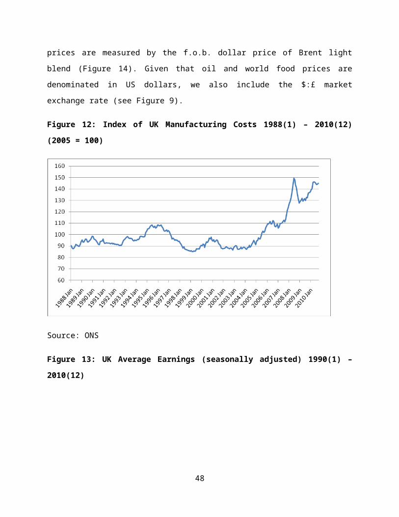
Figure 22: Simulated Food Price Inflation following a 20% Permanent Depreciation

in the $:£ Exchange Rate in January 2010

In summary, the forecasting models that have been developed allow a wide range of

scenarios to be considered in addition to the generation of food inflation forecasts

themselves. The discussion of the scenarios has also highlighted two important features of

UK food price inflation. First, the impact of the drivers on food price inflation is relatively

modest and that because of the inelastic responses large and persistent changes in the

drivers are required to cause rapid food price inflation. Of course, the fact that some of

these drivers, principally world food commodity prices, are prone to such violent swings

simply underlines the importance of the models that have been developed. Second, food

price inflation lags movement in these drivers by at least three months suggesting that, to

the extent that the size and duration of shocks are known, food price inflation is to a large

degree predictable.

50

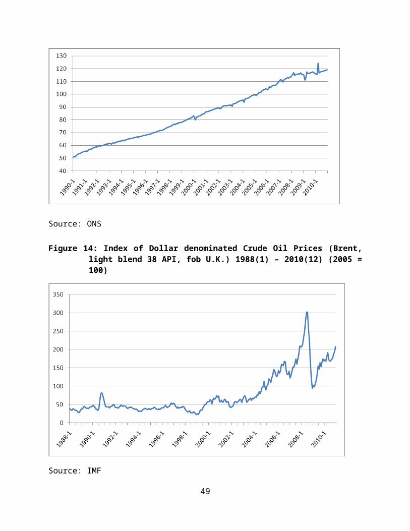
Section 5: Conclusions

This report has outlined a basis for forecasting domestic food prices in the UK. This is a

topic of considerable importance to policymakers and other stakeholder groups and an

issue that raises not inconsiderable challenges for economists. Broadly speaking, it is an

issue that has been relatively under-explored in that, while the focus on world commodity

prices has been the subject of considerable academic debate and modelling efforts, the

links between world prices and domestic price inflation has received much less attention.

In addition, in dealing with the time series properties of the commodity and food price data

(as well as that of other drivers), the econometric approach required to deal with these

issues involved employing modern econometric techniques. Only when the time series

properties of the data are fully accounted for and the vertical linkages between world and

domestic prices modelled in a consistent long-run framework, can we ensure that the

model which underlies the forecasting exercises is both theoretically consistent and

appropriate for the issues at hand.

On the basis of a vector autoregressive model we have identified the long-run drivers of

domestic food prices to be world commodity prices, the Dollar-Sterling exchange rate,

unemployment, labour costs and the price of oil. We find that food price inflation is

relatively unresponsive to changes in these drivers. The most important determinant of

food price inflation is world food prices with exchanges rates also exerting a significant

effect. This model then forms the basis for forecasting. We have shown that the in-sample

forecasting performance of the model is acceptable under any reasonable criterion. With

this, we have shown that the model can be used to forecast the outcomes of alternative

scenarios. The forecasts are presented either as point estimates or in the form of a range in

which we would forecast the expected price effects to lie. As such, the model here provides

an important tool for policymakers keen to understand the main drivers of food price

inflation in the UK and how domestic food prices will likely respond to a change in these

underlying drivers in both the short and long term.

51

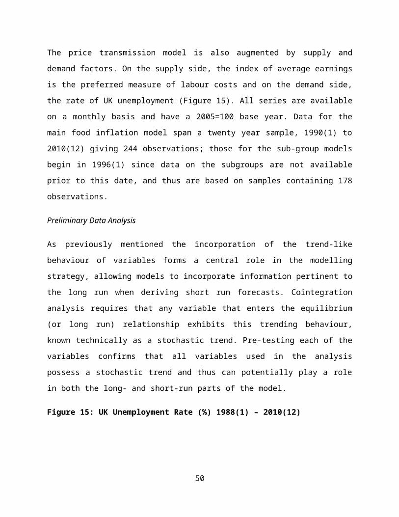
Appendix 1: References

Abbott, P., Hurt, C. and Tyner, W. (2008) “What’s Driving Food Prices.” Farm Foundation, July.

Ardeni, P.G. (1989) “Does the Law of One Price Really Hold for Commodity Prices?” American Journal of Agricultural Economics, 71: 303-328

Baffes, J. (1991) “Some Further Evidence on the Law of One Price” American Journal of Agricultural Economics, 4: 21-37

Ball, L. and N. G. Mankiw, (1994). “Asymmetric Price Adjustment and Economic Fluctuations,” Economic Journal 104:247-261.

Barrett, C. B. (2001) “Measuring Efficiency and Integration in International Agricultural Markets” Review of Agricultural Economics, 23: 19-32.

Blanchard, O. and J. Gali (2007) “The Macroeconomic Effects of Oil Price Shocks: Why are the 2000s So Different from the 1970s?” NBER Working Paper No. 13368.

Bukeviciute, L., A. Dierx and F. Ilzkovit (2009) “The Functioning of the Food Supply Chain and its Effect on Food Prices in the European Union” European Economy Occasional Papers, No. 47.

Conceicao, P. and Mendoza, R.U. (2009) “Anatomy of a Global Food Crisis” Third World Quarterly, 30(6): 1159-1182

DEFRA (2008) “Ensuring the UK’s Food Security in a Changing World” Discussion paper, London, July.

De Gregorio, J., O. Landerretche and C. Neilson (2007) “Another Pass-Through Bites the Dust: Oil Prices and Inflation” Bank of Chile Working Paper, No. 417.

FAO (2003). “Market Integration and Price Transmission in Selected Food and Cash Crop Markets of Developing Countries: Review and Applications”, by Rapsomanikis, G., Hallam, D., and P. Conforti, in Commodity Market Review 2003-2004., Commodities and Trade Division, FAO, Rome.

FAO (2009) The State of Agricultural Commodity Markets. FAO, Rome.

Ferrucci, G., R. Jiménez-Rodriquez and L. Onorante (2010) “Food Price Transmission in the Euro Area: The Role of Asymmetries and Non-Linearities” European Central Bank Working Paper, No. 1168

Fuglie, K.O. (2008) “Is a Slowdown in Agricultural Productivity Growth Contributing to the Rise in Commodity Prices?” Agricultural Economics, 39: 431-441.

52

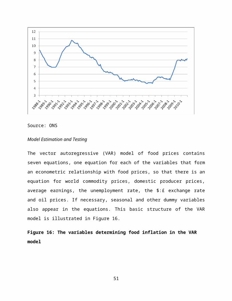
Gardner, B. (1975) 'The Farm-Retail Spread in a Competitive Industry' American Journal of Agricultural Economics, 65: 399-409.

Gilbert, C. L. (2010) “How to Understand High Food Prices”, Journal of Agricultural Economics, 61: 398-425.

Hamilton, J. (1996) “This is What Happened to the Oil Price-Macroeconomy Relationship” Journal of Monetary Economics, 38: 215-220.

Hathaway, D, (1974) “Food Prices and Inflation” Brookings Papers on Economic Activity 1, pp. 63–109

HMG (2009) The 2007/08 Agricultural Price Spikes: Causes and Policy Implications . Global Food Markets Group. HM Government, London.

International Monetary Fund (2008) “Is Inflation Back? Commodity Prices and Inflation” Chapter 3 World Economic Outlook.

Irwin. S., Sanders, D. And Merrin, R. (2009) “Devil of Angel? The Role of Speculation in the Recent Commodity Price Boom (and Bust)” Journal of Agricultural and Applied Economics 41: 377-391

Kinnucan, H.W. and O.D. Forker (1987) “Asymmetry in Farm-Retail Prices for Major Dairy Products” American Journal of Agricultural Economics, 69: 307-328.

Lloyd, T.A., McCorriston, S., Morgan, C.W. and Rayner, A.J. (2006) “Food Scares, Market Power and Price Transmission: the UK BSE Crisis”, European Review of Agricultural Economics, 33(2), 119-47.

McCorriston, S., C.W. Morgan and A.J. Rayner (1998) 'Processing Technology, Market Power and Price Transmission' Journal of Agricultural Economics, 49: 185-201.

Meyer, J. and S. von Cramon-Taubadel (2004) “Asymmetric Price Transmission: A Survey” Journal of Agricultural Economics, 55: 581-611.

Meyers, W.H. and Meyer, S. (2008) “Causes and Implications of the Food Price Surge”, World Economic Situation and Prospects 2009, UN Department for Economic and Social Affairs.

Mitchell, D. (2008) “A Note on Rising Food Prices”, World Bank Development Prospects Group, Policy Research Working Paper 4682, July.

Nakamura, E. and J. Steinsson (2008) ‘Five Facts About Prices: a Re-evaluation of Menu Cost Models’, Quarterly Journal of Economics 123: 1415-1464.

OECD (2008) “Rising Food prices: Causes and Consequences”. OECD, Paris.

53

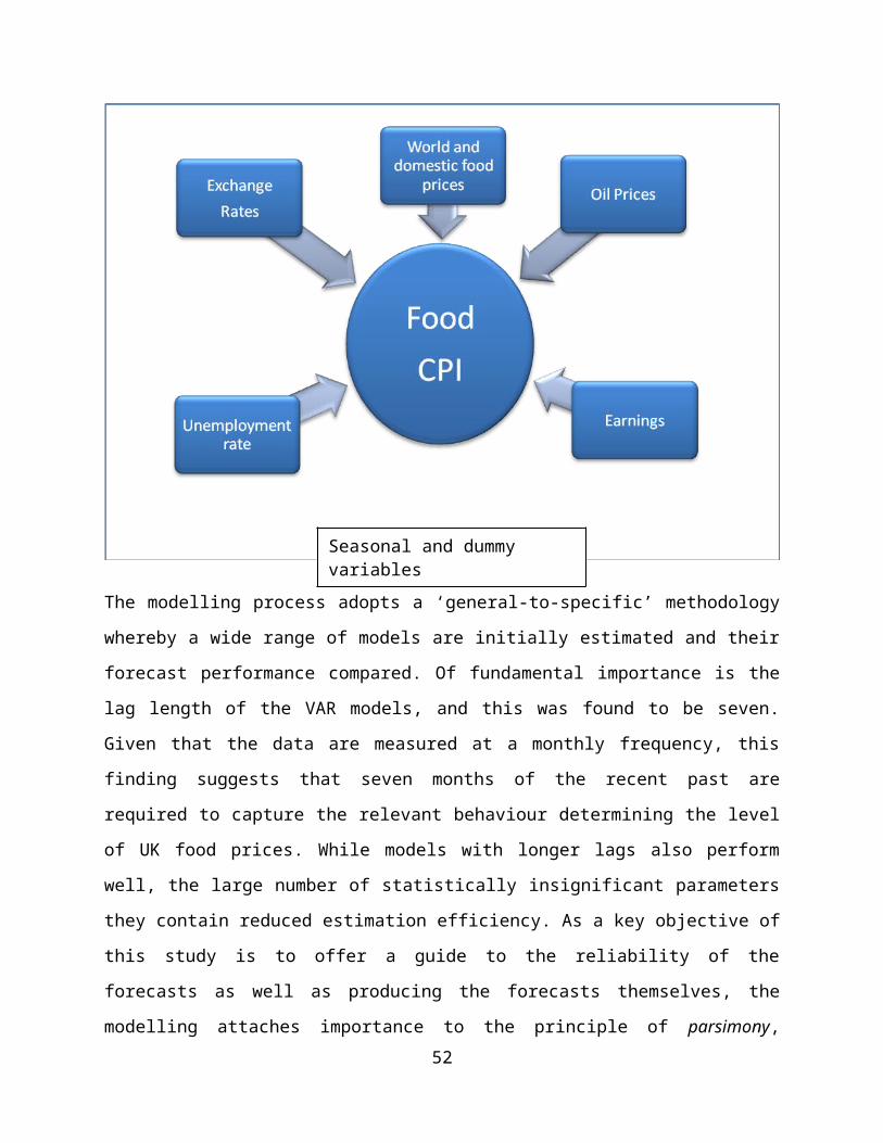
ONS (2007) Consumer Price Indices Technical Manual, Office for National Statistics, London (May)

Piesse, J. and Thirtle, C. (2009) “Three Bubbles and a Panic: An Explanatory Review of Recent Food Commodity Price Events” Food Policy, 34: 119-129.

Sánjuan, A.I. and P.J. Dawson (2003) “Price Transmission, BSE and Structural Breaks in the UK Meat Sector” European Review of Agricultural Economics, 30: 155-172.

Sarris, A. (2008) “Agricultural Commodity Markets and Trade: Price Spikes or Trends?” Presentation at “The Food Crisis of 2008: Lesson for the Future” Conference at Imperial College, 28th October

Shioji, E. and T. Uchino (2009) “Pass-Through of Oil prices to Japanese Domestic Prices” Forthcoming in T. Ito and A.K. Rose (eds.) Commodity Prices and Markets, NBER.

Sumner, D. (2009) “Recent Commodity Price Movements in Historical Perspective” American Journal of Agricultural Economics, 91(1) pp 1-7.

Trostle, R. (2008) “Global Agricultural Supply and Demand: Factors Contributing to the Recent Increase in Food Commodity Prices”, A Report from the Economic Research Service, United States Department of Agriculture, WRS-0801, July.

Vavra, P. and B.K.Goodwin (2005) “Analysis of Price Transmission Along the Food Chain” OECD Food, Agriculture and Fisheries Working Papers, No.3.

Wiggins, S. and Levy, S. (2008) “Rising Food Prices: Cause for Concern” ODI Natural Resources Briefing Paper 115, July.

Wiggins, S. and Keats, S. (2009) “Volatile World Food Prices and their Implications” ODI working paper, London, 7th September.

Wohlgenenant, M.K. (2001) “Marketing Margins: Empirical Analysis” in B.L. Gardner and G. Rausser (eds.) Handbook of Agricultural Economics, Volume 1. Elsevier, North-Holland, Amsterdam.

54

Appendix 2: Listing of the Fitted Models

Food Price Model

Data file is Food_price_forecasts.xls-----------------------------------------------------------------------System of Equations for 1: UKFCPI (Logs)2: WFPI (Logs)3: UKPPI (Logs)4: Poil (Logs)5: ER1 (Logs)6: Earn (Logs)7: UR (Logs)

Variables flagged with #LOG in Data Descriptions enter in logarithmic form.Estimation in differenced data (unit root imposed), including Type 1 regressors: Dummy_1 Month_2 Month_3 Month_4 Month_5 Month_6 Month_7 Month_8 Month_9 Month_10 Month_11 Month_12244 observations (33-276, dates 1990, Mth 9 to 2010, Mth 12)used for estimationwith 8 pre-sample observations.Estimation Method: Least Generalized VarianceVector-ARIMA(7,1,0), Linear ECM

Strong convergenceiteration time: 5.79 Log Likelihood = 5926.63 Schwarz Criterion = 5511.6 Hannan-Quinn Criterion = 5669.29 Akaike Criterion = 5775.63

Error Correlation Matrix Equation 1 Equation 2 Equation 3 Equation 4 Equation 5Equation 1 1.0000Equation 2 -0.021663 1.0000Equation 3 0.24873 0.11484 1.0000Equation 4 0.060738 0.23957 0.042608 1.0000Equation 5 -0.095299 0.32122 0.033174 0.078465 1.0000Equation 6 -0.074821 -0.015362 0.076325 0.073870 -0.024403Equation 7 0.10977 -0.069384 0.016637 0.066772 0.027382 Equation 6 Equation 7Equation 6 1.0000Equation 7 0.0053498 1.0000

Estimate Std. Err. t Ratio p-ValueEquilibrium Relation 1UKFCPI (Logs) 1 Fixed WFPI (Logs) -0.63351 0.19146 -3.309 0.001

55

ER1 (Logs) 0.50909 0.15961 3.19 0.002Earn (Logs) -0.2325 0.12115 -1.919 0.056UR (Logs) 0.15869 0.11099 1.43 0.154

Equilibrium Relation 2WFPI (Logs) 1 Fixed Poil (Logs) -0.55303 0.14219 -3.889 0poil_dum (Logs) -0.09175 0.03592 -2.554 0.011

Equation 1, for UKFCPI (Logs):[2]Intercept 0.14726 0.05199 2.832 0.005[1]Month_2 0.00186 0.00103 1.808 0.072[1]Month_3 0.00234 0.00102 2.291 0.023[1]Month_5 0.00804 0.00101 7.957 0[1]Month_6 0.00758 0.00105 7.223 0[1]Month_9 -0.00334 0.00117 -2.855 0.005[1]Month_10 -0.00558 0.00123 -4.533 0[1]Month_11 -0.00354 0.00116 -3.053 0.003ECM1 -0.04552 0.01719 -2.648 0.009AR1(1,3) 0.01498 0.01603 0.934 0.351AR1(1,7) 0.04251 0.02706 1.571 0.118AR2(1,2) -0.03341 0.01508 -2.216 0.028AR2(1,3) 0.043 0.01532 2.807 0.005AR2(1,4) -0.00773 0.00409 -1.891 0.06AR2(1,5) 0.02947 0.0164 1.797 0.074AR2(1,6) -0.04114 0.03788 -1.086 0.279AR2(1,7) 0.0294 0.02609 1.127 0.261AR3(1,1) -0.17909 0.06097 -2.937 0.004AR3(1,3) 0.07399 0.01629 4.542 0AR3(1,4) -0.0098 0.00412 -2.378 0.018AR3(1,7) 0.02642 0.02595 1.018 0.31AR4(1,2) -0.03912 0.01435 -2.726 0.007AR4(1,4) 0.0101 0.00401 2.518 0.013AR4(1,5) 0.03373 0.01647 2.048 0.042AR4(1,6) 0.15334 0.03891 3.941 0AR5(1,1) -0.12412 0.06249 -1.986 0.048AR5(1,3) 0.05141 0.0161 3.193 0.002AR5(1,5) -0.01509 0.01633 -0.924 0.357AR5(1,7) -0.04209 0.02646 -1.591 0.113AR6(1,2) 0.01954 0.01431 1.366 0.173AR6(1,4) 0.00458 0.00397 1.154 0.25AR6(1,6) 0.06702 0.03856 1.738 0.084AR6(1,7) 0.03067 0.02637 1.163 0.246AR7(1,2) -0.04272 0.01396 -3.06 0.002AR7(1,7) -0.02918 0.02634 -1.108 0.269 Sum of Squares = 0.0062 R-Squared = 0.9983 R-Bar-Squared = 0.9981 Residual SD = 0.0053 Residual Skewness = -0.0102 Residual Kurtosis = 3.0055 Jarque-Bera Test = 0.0046 {0.998}Box-Pierce (residuals): Q(5) = 5.0978 {0.404}Box-Pierce (squared residuals): Q(12) = 43.7339 {0}

Equation 2, for WFPI (Logs):[2]Intercept 0.07761 0.05555 1.397 0.164ECM2 -0.0351 0.01805 -1.944 0.053AR1(2,2) 0.40239 0.06223 6.466 0AR4(2,4) 0.02499 0.01907 1.31 0.191AR5(2,2) -0.12877 0.06135 -2.099 0.037AR5(2,4) -0.03035 0.01856 -1.635 0.103

56

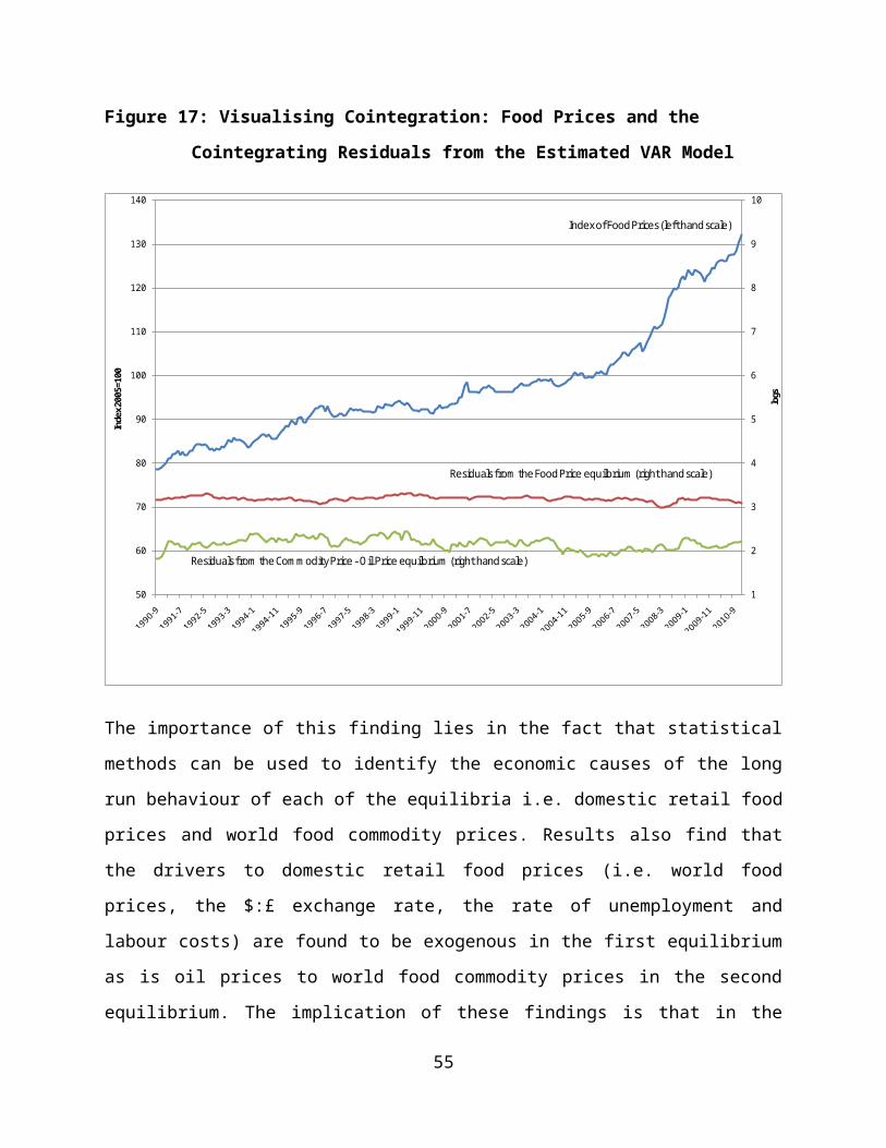
AR7(2,2) -0.10735 0.06156 -1.744 0.083 Sum of Squares = 0.1597 R-Squared = 0.9825 R-Bar-Squared = 0.9809 Residual SD = 0.0268 Residual Skewness = -0.5309 Residual Kurtosis = 6.4918 Jarque-Bera Test = 135.417 {0}Box-Pierce (residuals): Q(5) = 4.8173 {0.439}Box-Pierce (squared residuals): Q(12) = 16.5188 {0.169}

Equation 3, for UKPPI (Logs):[2]Intercept 0.00355 0.00167 2.123 0.035[1]Month_2 0.00746 0.00411 1.815 0.071[1]Month_3 0.01108 0.00409 2.709 0.007[1]Month_5 -0.00525 0.00376 -1.397 0.164[1]Month_7 -0.04031 0.00455 -8.858 0[1]Month_8 -0.01899 0.00489 -3.884 0[1]Month_9 -0.02003 0.00532 -3.764 0[1]Month_10 -0.02424 0.00556 -4.359 0[1]Month_11 -0.01116 0.00521 -2.142 0.033[1]Month_12 -0.01892 0.0045 -4.204 0AR1(3,1) 0.57586 0.23644 2.436 0.016AR1(3,2) 0.13463 0.05451 2.47 0.014AR1(3,3) -0.16517 0.0635 -2.601 0.01AR1(3,4) -0.02008 0.01582 -1.269 0.206AR1(3,7) -0.08941 0.09241 -0.968 0.334AR2(3,2) 0.06104 0.05696 1.072 0.285AR2(3,4) -0.02542 0.0166 -1.531 0.127AR3(3,3) 0.09574 0.06037 1.586 0.114AR3(3,4) -0.01675 0.01596 -1.049 0.295AR4(3,1) -0.54225 0.23354 -2.322 0.021AR5(3,3) 0.10313 0.06047 1.706 0.089AR5(3,5) -0.11036 0.05953 -1.854 0.065AR5(3,6) -0.62686 0.15624 -4.012 0AR6(3,1) -0.20783 0.22826 -0.91 0.364AR7(3,3) 0.08287 0.05954 1.392 0.165AR7(3,4) 0.0394 0.01522 2.589 0.01 Sum of Squares = 0.1025 R-Squared = 0.978 R-Bar-Squared = 0.976 Residual SD = 0.0215 Residual Skewness = -0.2966 Residual Kurtosis = 6.7349 Jarque-Bera Test = 145.396 {0}Box-Pierce (residuals): Q(5) = 12.6544 {0.027}Box-Pierce (squared residuals): Q(12) = 8.6637 {0.731}

Equation 4, for Poil (Logs):[2]Intercept 0.00384 0.00557 0.689 0.492AR1(4,2) 0.41406 0.21841 1.896 0.059AR1(4,4) 0.15337 0.06069 2.527 0.012AR2(4,2) 0.41219 0.21016 1.961 0.051AR4(4,4) -0.11707 0.06123 -1.912 0.057AR5(4,2) 0.24734 0.21485 1.151 0.251AR5(4,4) -0.06745 0.06418 -1.051 0.294AR6(4,2) 0.25432 0.22999 1.106 0.27AR6(4,4) -0.1193 0.06097 -1.957 0.052AR7(4,2) -0.24362 0.21839 -1.116 0.266 Sum of Squares = 1.6509 R-Squared = 0.9825 R-Bar-Squared = 0.9809 Residual SD = 0.0862

57

Residual Skewness = -0.0974 Residual Kurtosis = 3.0161 Jarque-Bera Test = 0.3886 {0.823}Box-Pierce (residuals): Q(5) = 12.4036 {0.03}Box-Pierce (squared residuals): Q(12) = 39.2029 {0}

Equation 5, for ER1 (Logs):[2]Intercept -0.00583 0.00216 -2.699 0.007AR1(5,2) 0.11343 0.05345 2.122 0.035AR1(5,3) -0.10311 0.05669 -1.819 0.07AR1(5,4) 0.03875 0.01506 2.573 0.011AR1(5,5) 0.2739 0.06251 4.382 0AR1(5,6) 0.30692 0.14072 2.181 0.03AR1(5,7) -0.21942 0.09642 -2.276 0.024AR2(5,5) -0.23507 0.06131 -3.834 0AR2(5,7) -0.09957 0.09682 -1.028 0.305AR3(5,1) 0.51145 0.23443 2.182 0.03AR3(5,3) -0.11777 0.0598 -1.969 0.05AR3(5,5) 0.08492 0.05832 1.456 0.147AR3(5,6) 0.49828 0.15961 3.122 0.002AR4(5,1) -0.38149 0.2179 -1.751 0.081AR4(5,4) 0.0183 0.01529 1.197 0.233AR4(5,6) 0.2601 0.1676 1.552 0.122AR5(5,5) -0.0942 0.05719 -1.647 0.101AR5(5,6) 0.29199 0.15176 1.924 0.056AR5(5,7) 0.09487 0.09663 0.982 0.327AR6(5,1) 0.25779 0.22207 1.161 0.247AR6(5,2) -0.07312 0.04975 -1.47 0.143AR6(5,4) -0.02968 0.01488 -1.995 0.047AR7(5,1) -0.4255 0.21845 -1.948 0.053AR7(5,4) -0.01438 0.01505 -0.956 0.34AR7(5,5) -0.10079 0.05625 -1.792 0.075AR7(5,6) 0.20337 0.13879 1.465 0.144AR7(5,7) 0.09297 0.09329 0.997 0.32 Sum of Squares = 0.0934 R-Squared = 0.9604 R-Bar-Squared = 0.9567 Residual SD = 0.0205 Residual Skewness = -0.5833 Residual Kurtosis = 4.9322 Jarque-Bera Test = 51.7901 {0}Box-Pierce (residuals): Q(5) = 8.7191 {0.121}Box-Pierce (squared residuals): Q(12) = 20.9653 {0.051}

Equation 6, for Earn (Logs):[2]Intercept 0.00612 0.0009 6.796 0AR1(6,2) -0.02981 0.01877 -1.588 0.114AR1(6,6) -0.56017 0.0613 -9.138 0AR2(6,5) 0.02787 0.02205 1.264 0.208AR2(6,6) -0.3472 0.06848 -5.07 0AR2(6,7) 0.05194 0.03587 1.448 0.149AR3(6,1) -0.09013 0.08927 -1.01 0.314AR3(6,4) 0.01443 0.00584 2.471 0.014AR3(6,6) -0.16301 0.07004 -2.327 0.021AR4(6,2) 0.04104 0.0201 2.042 0.042AR4(6,5) 0.03149 0.02326 1.354 0.177AR4(6,6) -0.05357 0.06214 -0.862 0.39AR4(6,7) -0.09393 0.03601 -2.608 0.01AR5(6,1) 0.19135 0.09031 2.119 0.035AR6(6,2) -0.0386 0.01937 -1.993 0.047AR6(6,4) -0.01751 0.00566 -3.094 0.002AR6(6,6) 0.07972 0.05813 1.371 0.172AR7(6,3) -0.04683 0.02318 -2.02 0.045

58

AR7(6,6) 0.1325 0.0607 2.183 0.03 Sum of Squares = 0.0138 R-Squared = 0.999 R-Bar-Squared = 0.9989 Residual SD = 0.0079 Residual Skewness = 0.3903 Residual Kurtosis = 14.418 Jarque-Bera Test = 1331.63 {0}Box-Pierce (residuals): Q(5) = 3.8686 {0.568}Box-Pierce (squared residuals): Q(12) = 20.7426 {0.054}

Equation 7, for UR (Logs):[2]Intercept -0.00333 0.00117 -2.85 0.005AR1(7,1) 0.22926 0.14735 1.556 0.121AR1(7,2) 0.0451 0.03418 1.319 0.188AR1(7,3) 0.06082 0.04025 1.511 0.132AR1(7,5) -0.09055 0.0396 -2.287 0.023AR1(7,7) 0.21051 0.06267 3.359 0.001AR2(7,1) 0.29091 0.15681 1.855 0.065AR2(7,3) -0.07879 0.04036 -1.952 0.052AR2(7,4) 0.01309 0.00973 1.345 0.18AR2(7,7) 0.11951 0.06453 1.852 0.065AR3(7,1) 0.19162 0.149 1.286 0.2AR3(7,3) -0.0888 0.03913 -2.269 0.024AR4(7,1) 0.31124 0.14878 2.092 0.038AR4(7,6) 0.10349 0.09375 1.104 0.271AR4(7,7) 0.17993 0.0616 2.921 0.004AR5(7,4) -0.01356 0.00961 -1.411 0.16AR6(7,1) 0.14524 0.14426 1.007 0.315AR6(7,4) 0.01879 0.0098 1.917 0.056AR6(7,6) 0.2132 0.09445 2.257 0.025AR7(7,2) -0.04098 0.03229 -1.269 0.206AR7(7,7) 0.14498 0.06004 2.415 0.017 Sum of Squares = 0.0379 R-Squared = 0.9977 R-Bar-Squared = 0.9975 Residual SD = 0.013 Residual Skewness = 0.3113 Residual Kurtosis = 3.6255 Jarque-Bera Test = 7.9172 {0.019}Box-Pierce (residuals): Q(5) = 8.1382 {0.149}Box-Pierce (squared residuals): Q(12) = 36.4192 {0}

59

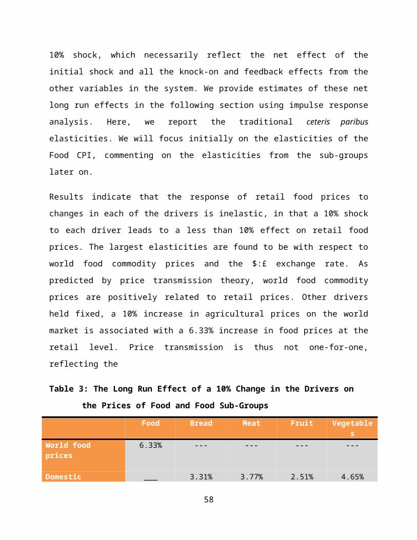
Bread Price Model

System of Equations for

1: BCPI (Logs)2: BAPI (Logs)3: ER1 (Logs)4: Earn (Logs)Variables flagged with #LOG in Data Descriptions enter in logarithmic form.Estimation in differenced data (unit root imposed), including Type 1 regressors: Dummy_1 Month_2 Month_3 Month_4 Month_5 Month_6 Month_7 Month_8 Month_9 Month_10 Month_11 Month_12173 observations (104-276, dates 1996, Mth 8 to 2010, Mth 12)used for estimationwith 7 pre-sample observations.Estimation Method: Least Generalized VarianceVector-ARIMA(6,1,0), Linear ECM

Log Likelihood = 2433.35 Schwarz Criterion = 2268.44 Hannan-Quinn Criterion = 2328.41 Akaike Criterion = 2369.35

Error Correlation Matrix Equation 1 Equation 2 Equation 3 Equation 4Equation 1 1.0000Equation 2 0.028557 1.0000Equation 3 -0.14202 0.20006 1.0000Equation 4 -0.021871 0.027011 0.0089313 1.0000

Estimate Std. Err. t Ratio p-ValueEquilibrium Relation BCPI (Logs) 1 Fixed BAPI (Logs) -0.33059 0.05789 -5.711 0ER1 (Logs) 0.23391 0.10445 2.239 0.027Earn (Logs) -0.52535 0.07378 -7.121 0

Equation 1, for BCPI (Logs):[2]Intercept 0.08937 0.04732 1.889 0.061[1]Month_2 0.00312 0.00121 2.577 0.011[1]Month_6 0.00185 0.00164 1.125 0.262[1]Month_7 0.00158 0.0017 0.928 0.355[1]Month_10 0.00146 0.00119 1.226 0.222[1]Month_11 0.00268 0.00168 1.597 0.112

60

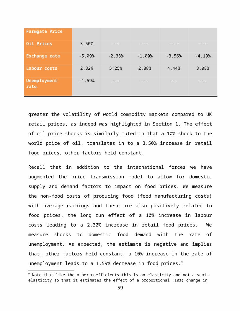
[1]Month_12 0.00653 0.00145 4.507 0ECM1 -0.05231 0.01492 -3.506 0.001AR2(1,2) 0.01074 0.00892 1.204 0.23AR2(1,4) 0.04754 0.04514 1.053 0.294AR3(1,1) 0.13975 0.08534 1.638 0.104AR3(1,4) 0.07484 0.05314 1.408 0.161AR4(1,1) -0.16867 0.08642 -1.952 0.053AR4(1,4) 0.08474 0.0778 1.089 0.278AR5(1,1) -0.12209 0.07505 -1.627 0.106AR5(1,3) -0.02134 0.0199 -1.072 0.285AR5(1,4) 0.14776 0.05604 2.637 0.009AR6(1,1) 0.09184 0.08733 1.052 0.295AR6(1,2) -0.01492 0.00908 -1.644 0.102AR6(1,4) 0.13415 0.04779 2.807 0.006 Sum of Squares = 0.0044 R-Squared = 0.9976 R-Bar-Squared = 0.9973 Residual SD = 0.0053 Residual Skewness = -0.2323 Residual Kurtosis = 3.6912 Jarque-Bera Test = 5.0005 {0.082}Box-Pierce (residuals): Q(6) = 6.2641 {0.394}Box-Pierce (squared residuals): Q(12) = 14.3076 {0.282}

Equation 2, for BAPI (Logs):[2]Intercept 0.01939 0.00841 2.306 0.022[1]Month_3 -0.02186 0.00887 -2.464 0.015[1]Month_4 -0.00964 0.00885 -1.089 0.278[1]Month_6 -0.02594 0.01119 -2.319 0.022[1]Month_8 -0.06087 0.0137 -4.443 0[1]Month_11 -0.01039 0.00655 -1.586 0.115[1]Month_12 -0.0184 0.00836 -2.201 0.029AR1(2,1) -0.81322 0.89501 -0.909 0.365AR1(2,2) 0.30546 0.07949 3.843 0AR1(2,4) -0.92013 0.42916 -2.144 0.034AR2(2,1) -0.97881 1.05309 -0.929 0.354AR2(2,2) 0.12478 0.0713 1.75 0.082AR2(2,4) -0.63509 0.48289 -1.315 0.19AR3(2,2) -0.07648 0.05226 -1.463 0.145AR3(2,4) -0.99709 0.55165 -1.807 0.073AR4(2,4) -2.06496 1.05534 -1.957 0.052AR5(2,2) 0.07994 0.07489 1.067 0.287AR5(2,3) -0.23376 0.16518 -1.415 0.159AR6(2,3) 0.2542 0.16867 1.507 0.134 Sum of Squares = 0.423 R-Squared = 0.9705 R-Bar-Squared = 0.9677 Residual SD = 0.0519 Residual Skewness = -0.5996 Residual Kurtosis = 7.2924 Jarque-Bera Test = 143.175 {0}Box-Pierce (residuals): Q(6) = 8.6578 {0.194}Box-Pierce (squared residuals): Q(12) = 22.8782 {0.029}

Equation 3, for ER1 (Logs):[2]Intercept 0.00203 0.002 1.014 0.312AR1(3,4) 0.38268 0.16481 2.322 0.022

61

AR2(3,2) 0.037 0.02748 1.347 0.18AR4(3,1) -0.65127 0.32602 -1.998 0.047AR5(3,1) -0.86132 0.38843 -2.217 0.028AR6(3,2) 0.07007 0.03032 2.311 0.022AR6(3,3) -0.14801 0.08157 -1.814 0.072AR6(3,4) -0.24158 0.13363 -1.808 0.073 Sum of Squares = 0.0699 R-Squared = 0.9605 R-Bar-Squared = 0.9567 Residual SD = 0.0211 Residual Skewness = 0.0485 Residual Kurtosis = 3.4301 Jarque-Bera Test = 1.4012 {0.496}Box-Pierce (residuals): Q(6) = 17.27 {0.008}Box-Pierce (squared residuals): Q(12) = 7.3458 {0.834}

Equation 4, for Earn (Logs):[2]Intercept 0.0097 0.00252 3.85 0AR1(4,1) -0.32136 0.15445 -2.081 0.039AR1(4,2) -0.019 0.01328 -1.431 0.155AR1(4,4) -0.59861 0.17268 -3.467 0.001AR2(4,3) 0.06357 0.03078 2.065 0.041AR2(4,4) -0.48666 0.14898 -3.267 0.001AR3(4,1) -0.19004 0.17811 -1.067 0.288AR3(4,4) -0.32769 0.14314 -2.289 0.023AR4(4,2) 0.02264 0.01007 2.249 0.026AR4(4,3) 0.06566 0.04861 1.351 0.179AR4(4,4) -0.21862 0.11767 -1.858 0.065AR5(4,2) 0.0398 0.01444 2.756 0.007AR5(4,3) -0.05356 0.03482 -1.538 0.126AR5(4,4) -0.17639 0.09119 -1.934 0.055 Sum of Squares = 0.0129 R-Squared = 0.9972 R-Bar-Squared = 0.997 Residual SD = 0.0091 Residual Skewness = 0.0377 Residual Kurtosis = 15.558 Jarque-Bera Test = 1136.82 {0}Box-Pierce (residuals): Q(6) = 3.4519 {0.75}Box-Pierce (squared residuals): Q(12) = 8.5361 {0.742}

62

Meat Price Model

System of Equations for

1: MCPI (Logs)2: MAPI (Logs)3: ER1 (Logs)4: Earn (Logs)Variables flagged with #LOG in Data Descriptions enter in logarithmic form.Estimation in differenced data (unit root imposed), including Type 1 regressors: Dummy_1 Month_2 Month_3 Month_4 Month_5 Month_6 Month_7 Month_8 Month_9 Month_10 Month_11 Month_12178 observations (99-276, dates 1996, Mth 3 to 2010, Mth 12)used for estimationwith 2 pre-sample observations.Estimation Method: Least Generalized VarianceVector-ARIMA(1,1,0), Linear ECM

Log Likelihood = 2572.89 Schwarz Criterion = 2453.71 Hannan-Quinn Criterion = 2497.21 Akaike Criterion = 2526.89

Error Correlation Matrix Equation 1 Equation 2 Equation 3 Equation 4Equation 1 1.0000Equation 2 -0.014483 1.0000Equation 3 -0.070318 -0.054501 1.0000Equation 4 -0.14652 0.18618 0.0047338 1.0000

Estimate Std. Err. t Ratio p-ValueEquilibrium Relation MCPI (Logs) 1 Fixed MAPI (Logs) -0.37712 0.03084 -12.228 0ER1 (Logs) 0.10026 0.04966 2.019 0.045Earn (Logs) -0.28813 0.0296 -9.734 0

Equation 1, for MCPI (Logs):[2]Intercept 0.36394 0.13382 2.72 0.007[1]Month_2 0.00158 0.00146 1.084 0.28[1]Month_3 0.00047 0.00338 0.138 0.89[1]Month_4 -0.00198 0.00328 -0.605 0.546[1]Month_5 0.00082 0.00366 0.225 0.822[1]Month_6 -0.00031 0.00397 -0.079 0.937

63

[1]Month_7 -0.00097 0.00409 -0.238 0.812[1]Month_8 -0.0007 0.0041 -0.171 0.865[1]Month_9 -0.00284 0.00408 -0.697 0.487[1]Month_10 -0.00381 0.00375 -1.015 0.312[1]Month_11 -0.00247 0.00353 -0.698 0.486[1]Month_12 0.00056 0.00288 0.195 0.846ECM1 -0.18071 0.04897 -3.69 0AR1(1,1) -0.00455 0.08885 -0.051 0.959AR1(1,2) -0.00409 0.0416 -0.098 0.922AR1(1,3) -0.01742 0.02737 -0.637 0.525AR1(1,4) -0.00814 0.07062 -0.115 0.908 Sum of Squares = 0.0118 R-Squared = 0.9923 R-Bar-Squared = 0.9918 Residual SD = 0.0084 Residual Skewness = 0.9636 Residual Kurtosis = 6.6007 Jarque-Bera Test = 123.706 {0}Box-Pierce (residuals): Q(11) = 16.5846 {0.121}Box-Pierce (squared residuals): Q(12) = 5.5816 {0.936}

Equation 2, for MAPI (Logs):[2]Intercept 0.00061 0.00148 0.412 0.681[1]Month_2 0.01817 0.00632 2.875 0.005[1]Month_3 0.02882 0.00874 3.298 0.001[1]Month_4 0.04262 0.00951 4.482 0[1]Month_5 0.03953 0.01035 3.82 0[1]Month_6 0.03604 0.01127 3.198 0.002[1]Month_7 0.00581 0.01203 0.483 0.63[1]Month_8 -0.00895 0.01149 -0.779 0.437[1]Month_9 -0.03065 0.01129 -2.715 0.007[1]Month_10 -0.04295 0.0105 -4.091 0[1]Month_11 -0.02667 0.00932 -2.861 0.005[1]Month_12 -0.00493 0.00609 -0.81 0.419AR1(2,1) 0.30211 0.179 1.688 0.093AR1(2,2) 0.32245 0.09031 3.57 0AR1(2,3) -0.02225 0.06036 -0.369 0.713AR1(2,4) -0.10023 0.14191 -0.706 0.481 Sum of Squares = 0.0587 R-Squared = 0.9888 R-Bar-Squared = 0.9881 Residual SD = 0.0188 Residual Skewness = -0.3944 Residual Kurtosis = 3.5495 Jarque-Bera Test = 6.8536 {0.032}Box-Pierce (residuals): Q(11) = 18.921 {0.063}Box-Pierce (squared residuals): Q(12) = 11.3225 {0.502}

Equation 3, for ER1 (Logs):[2]Intercept -0.00154 0.00179 -0.858 0.392AR1(3,1) 0.00827 0.19326 0.043 0.966AR1(3,2) 0.01698 0.07367 0.231 0.818AR1(3,3) 0.30479 0.10055 3.031 0.003AR1(3,4) 0.48353 0.12484 3.873 0 Sum of Squares = 0.0745 R-Squared = 0.9596 R-Bar-Squared = 0.9571

64

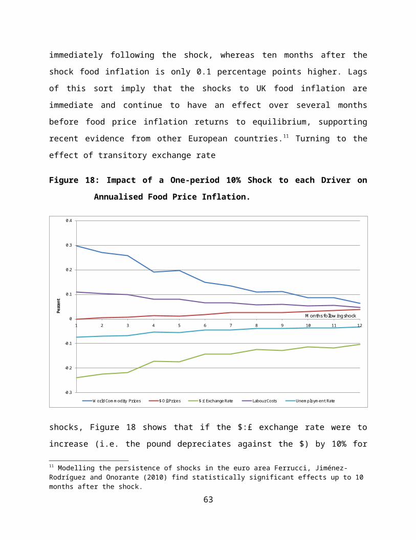
Residual SD = 0.0212 Residual Skewness = -0.2916 Residual Kurtosis = 3.8092 Jarque-Bera Test = 7.3799 {0.025}Box-Pierce (residuals): Q(11) = 8.3551 {0.681}Box-Pierce (squared residuals): Q(12) = 12.8699 {0.379}

Equation 4, for Earn (Logs):[2]Intercept 0.00424 0.00098 4.325 0AR1(4,1) 0.04107 0.09157 0.448 0.654AR1(4,2) -0.06996 0.06461 -1.083 0.28AR1(4,3) -0.01921 0.04594 -0.418 0.676AR1(4,4) -0.35013 0.19953 -1.755 0.081 Sum of Squares = 0.0169 R-Squared = 0.9967 R-Bar-Squared = 0.9965 Residual SD = 0.0101 Residual Skewness = 0.8305 Residual Kurtosis = 16.865 Jarque-Bera Test = 1446.22 {0}Box-Pierce (residuals): Q(11) = 18.6202 {0.068}Box-Pierce (squared residuals): Q(12) = 39.4032 {0}

65

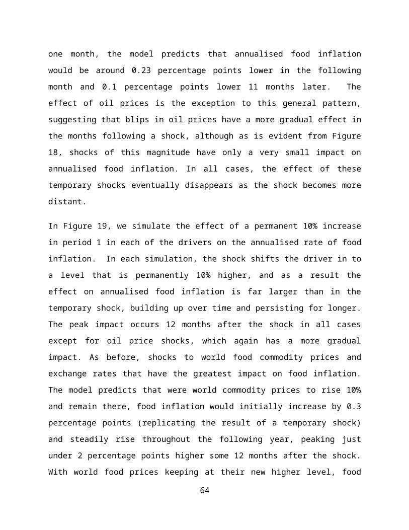
Fruit Price Model

System of Equations for

1: FCPI (Logs)2: FAPI (Logs)3: ER1 (Logs)4: Earn (Logs)Variables flagged with #LOG in Data Descriptions enter in logarithmic form.Estimation in differenced data (unit root imposed), including Type 1 regressors: Dummy_1 Month_2 Month_3 Month_4 Month_5 Month_6 Month_7 Month_8 Month_9 Month_10 Month_11 Month_12178 observations (99-276, dates 1996, Mth 3 to 2010, Mth 12)used for estimationwith 2 pre-sample observations.Estimation Method: Least Generalized VarianceVector-ARIMA(1,1,0), Linear ECM

Log Likelihood = 2125.48 Schwarz Criterion = 2006.3 Hannan-Quinn Criterion = 2049.8 Akaike Criterion = 2079.48

Error Correlation Matrix Equation 1 Equation 2 Equation 3 Equation 4Equation 1 1.0000Equation 2 0.18235 1.0000Equation 3 -0.11896 0.15550 1.0000Equation 4 0.0090371 0.028582 0.0045139 1.0000

Estimate Std. Err. t Ratio p-ValueEquilibrium Relation FCPI (Logs) 1 Fixed FAPI (Logs) -0.25061 0.07753 -3.232 0.001ER1 (Logs) 0.35543 0.08955 3.969 0Earn (Logs) -0.44423 0.06204 -7.16 0

Equation 1, for FCPI (Logs):[2]Intercept 0.64079 0.24888 2.575 0.011[1]Month_2 -0.0036 0.0058 -0.62 0.536[1]Month_3 -0.01394 0.00762 -1.829 0.069[1]Month_4 -0.01734 0.01003 -1.729 0.086[1]Month_5 0.01208 0.01333 0.906 0.366[1]Month_6 0.02445 0.01481 1.651 0.101[1]Month_7 -0.01953 0.01443 -1.354 0.178

66

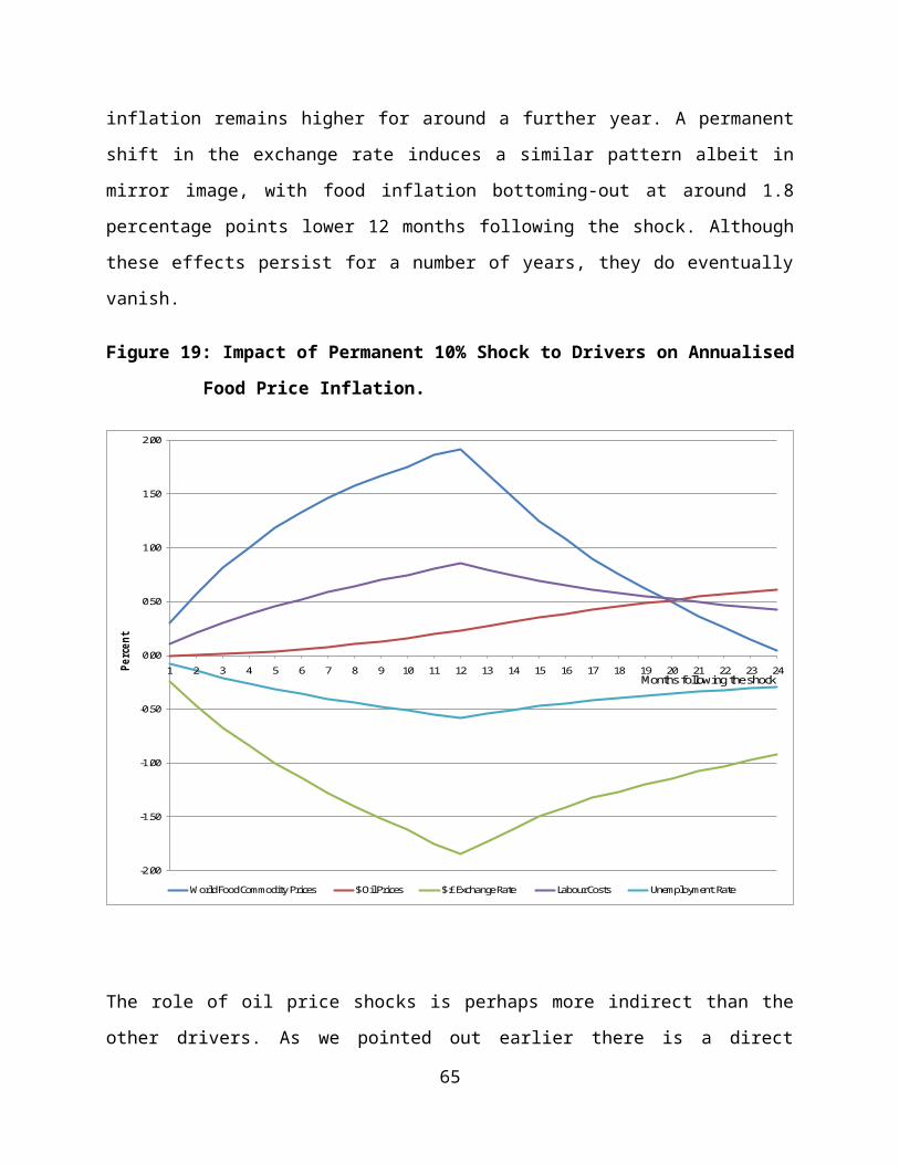
[1]Month_8 -0.01254 0.01307 -0.96 0.339[1]Month_9 -0.024 0.01257 -1.909 0.058[1]Month_10 -0.00083 0.01221 -0.068 0.946[1]Month_11 0.03052 0.0096 3.179 0.002[1]Month_12 0.04461 0.00613 7.277 0ECM1 -0.21215 0.07248 -2.927 0.004AR1(1,1) 0.01932 0.09196 0.21 0.834AR1(1,2) -0.03218 0.02217 -1.452 0.149AR1(1,3) -0.00392 0.07959 -0.049 0.961AR1(1,4) 0.1265 0.15171 0.834 0.406 Sum of Squares = 0.0754 R-Squared = 0.9537 R-Bar-Squared = 0.9507 Residual SD = 0.0213 Residual Skewness = 0.3313 Residual Kurtosis = 3.1752 Jarque-Bera Test = 3.4835 {0.175}Box-Pierce (residuals): Q(11) = 10.4417 {0.491}Box-Pierce (squared residuals): Q(12) = 8.5196 {0.743}

Equation 2, for FAPI (Logs):[2]Intercept 0.0048 0.00734 0.653 0.514[1]Month_2 0.02886 0.01828 1.579 0.116[1]Month_3 0.02269 0.02055 1.104 0.271[1]Month_4 0.03319 0.0279 1.19 0.236[1]Month_5 0.06535 0.02997 2.181 0.031[1]Month_6 -0.01583 0.044 -0.36 0.72[1]Month_7 -0.13435 0.03419 -3.93 0[1]Month_8 -0.05565 0.0306 -1.819 0.071[1]Month_9 -0.05958 0.02704 -2.203 0.029[1]Month_10 -0.02613 0.02277 -1.148 0.253[1]Month_11 -0.03985 0.01693 -2.354 0.02[1]Month_12 -0.00428 0.01498 -0.286 0.775AR1(2,1) -0.69769 0.34424 -2.027 0.044AR1(2,2) -0.41164 0.08565 -4.806 0AR1(2,3) -0.43401 0.28177 -1.54 0.125AR1(2,4) -0.53127 0.55161 -0.963 0.337 Sum of Squares = 1.4145 R-Squared = 0.698 R-Bar-Squared = 0.6789 Residual SD = 0.0922 Residual Skewness = -0.2409 Residual Kurtosis = 5.593 Jarque-Bera Test = 51.5877 {0}Box-Pierce (residuals): Q(11) = 15.8807 {0.146}Box-Pierce (squared residuals): Q(12) = 20.984 {0.051}

Equation 3, for ER1 (Logs):[2]Intercept -0.00126 0.00174 -0.722 0.472AR1(3,1) -0.09047 0.08507 -1.063 0.289AR1(3,2) 0.01144 0.01647 0.695 0.488AR1(3,3) 0.29482 0.09819 3.003 0.003AR1(3,4) 0.47056 0.12089 3.892 0 Sum of Squares = 0.0737 R-Squared = 0.96 R-Bar-Squared = 0.9575 Residual SD = 0.021

67

Residual Skewness = -0.3267 Residual Kurtosis = 3.7178 Jarque-Bera Test = 6.9881 {0.03}Box-Pierce (residuals): Q(11) = 7.4657 {0.76}Box-Pierce (squared residuals): Q(12) = 14.8722 {0.249}

Equation 4, for Earn (Logs):[2]Intercept 0.00429 0.00097 4.426 0AR1(4,1) -0.00056 0.04154 -0.013 0.989AR1(4,2) -0.00419 0.00476 -0.881 0.38AR1(4,3) -0.01534 0.04506 -0.341 0.734AR1(4,4) -0.37043 0.18772 -1.973 0.05 Sum of Squares = 0.0172 R-Squared = 0.9967 R-Bar-Squared = 0.9965 Residual SD = 0.0102 Residual Skewness = 0.9912 Residual Kurtosis = 18.5736 Jarque-Bera Test = 1827.96 {0}Box-Pierce (residuals): Q(11) = 18.4345 {0.072}Box-Pierce (squared residuals): Q(12) = 31.9046 {0.001}

68

Vegetables Price Model

System of Equations for

1: VCPI (Logs)2: VAPI (Logs)3: ER2 (Logs)4: Earn (Logs)Variables flagged with #LOG in Data Descriptions enter in logarithmic form.Estimation in differenced data (unit root imposed), including Type 1 regressors: Dummy_1 Month_2 Month_3 Month_4 Month_5 Month_6 Month_7 Month_8 Month_9 Month_10 Month_11 Month_12178 observations (99-276, dates 1996, Mth 3 to 2010, Mth 12)used for estimationwith 2 pre-sample observations.Estimation Method: Least Generalized VarianceVector-ARIMA(1,1,0), Linear ECM

Log Likelihood = 2208.08 Schwarz Criterion = 2088.9 Hannan-Quinn Criterion = 2132.4 Akaike Criterion = 2162.08

Error Correlation Matrix Equation 1 Equation 2 Equation 3 Equation 4Equation 1 1.0000Equation 2 0.38063 1.0000Equation 3 -0.18482 0.0085957 1.0000Equation 4 -0.090741 -0.13661 -0.12473 1.0000

Estimate Std. Err. t Ratio p-ValueEquilibrium Relation VCPI (Logs) 1 Fixed VAPI (Logs) -0.46538 0.10305 -4.516 0ER2 (Logs) 0.41934 0.0986 4.253 0Earn (Logs) -0.3077 0.07995 -3.849 0

Equation 1, for VCPI (Logs):[2]Intercept 0.77457 0.26616 2.91 0.004[1]Month_2 -0.00027 0.00711 -0.037 0.97[1]Month_3 0.00582 0.00916 0.635 0.526[1]Month_4 -0.009 0.01046 -0.861 0.391[1]Month_5 0.00344 0.01144 0.301 0.764[1]Month_6 -0.00736 0.01235 -0.596 0.552[1]Month_7 -0.02802 0.01272 -2.203 0.029

69

[1]Month_8 -0.03215 0.0127 -2.532 0.012[1]Month_9 -0.03652 0.012 -3.043 0.003[1]Month_10 -0.04558 0.01089 -4.186 0[1]Month_11 -0.04237 0.00925 -4.581 0[1]Month_12 -0.02454 0.00677 -3.624 0ECM1 -0.25885 0.05358 -4.831 0AR1(1,1) 0.01092 0.08191 0.133 0.894AR1(1,2) -0.00335 0.03366 -0.1 0.921AR1(1,3) -0.10005 0.13197 -0.758 0.449AR1(1,4) 0.10418 0.20517 0.508 0.612 Sum of Squares = 0.1098 R-Squared = 0.9667 R-Bar-Squared = 0.9646 Residual SD = 0.0257 Residual Skewness = 0.607 Residual Kurtosis = 4.2453 Jarque-Bera Test = 22.4332 {0}Box-Pierce (residuals): Q(11) = 8.9913 {0.623}Box-Pierce (squared residuals): Q(12) = 14.2251 {0.287}

Equation 2, for VAPI (Logs):[2]Intercept 0.0026 0.00554 0.469 0.639[1]Month_2 -0.05229 0.02005 -2.608 0.01[1]Month_3 -0.00718 0.0237 -0.303 0.762[1]Month_4 0.00923 0.02601 0.355 0.723[1]Month_5 0.00299 0.02787 0.107 0.915[1]Month_6 -0.03423 0.02908 -1.177 0.241[1]Month_7 -0.01968 0.02957 -0.665 0.507[1]Month_8 -0.05689 0.0293 -1.942 0.054[1]Month_9 -0.06458 0.02821 -2.289 0.023[1]Month_10 -0.08331 0.02622 -3.178 0.002[1]Month_11 -0.10249 0.02334 -4.391 0[1]Month_12 -0.06617 0.01908 -3.468 0.001AR1(2,1) -0.07443 0.20892 -0.356 0.722AR1(2,2) -0.13163 0.08144 -1.616 0.108AR1(2,3) -0.44371 0.34973 -1.269 0.206AR1(2,4) -0.14348 0.552 -0.26 0.795 Sum of Squares = 0.8119 R-Squared = 0.8278 R-Bar-Squared = 0.8169 Residual SD = 0.0698 Residual Skewness = 0.3815 Residual Kurtosis = 3.541 Jarque-Bera Test = 6.488 {0.039}Box-Pierce (residuals): Q(11) = 12.0991 {0.356}Box-Pierce (squared residuals): Q(12) = 4.1069 {0.981}

Equation 3, for ER2 (Logs):[2]Intercept -0.00085 0.00123 -0.69 0.491AR1(3,1) -0.02786 0.0474 -0.588 0.557AR1(3,2) 0.01056 0.01879 0.562 0.575AR1(3,3) 0.20405 0.07651 2.667 0.008AR1(3,4) 0.269 0.1138 2.364 0.019 Sum of Squares = 0.0407 R-Squared = 0.9694 R-Bar-Squared = 0.9675 Residual SD = 0.0156

70

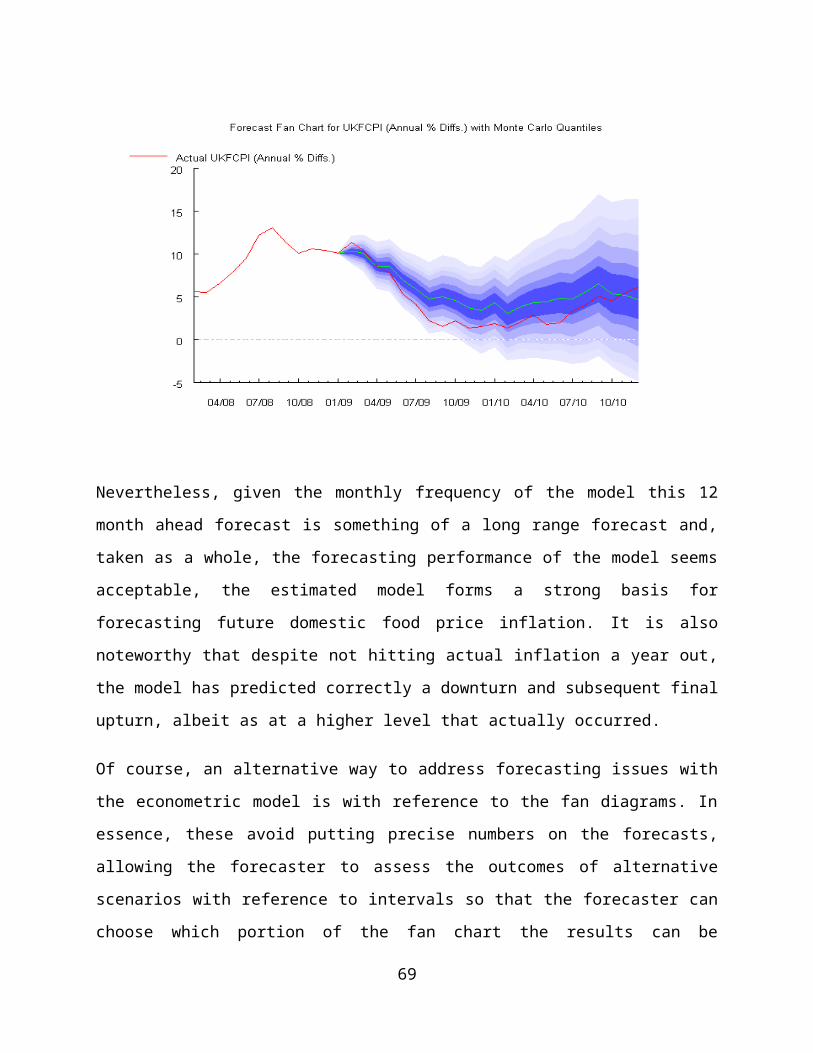
Residual Skewness = -0.4592 Residual Kurtosis = 4.9787 Jarque-Bera Test = 35.2952 {0}Box-Pierce (residuals): Q(11) = 5.1976 {0.921}Box-Pierce (squared residuals): Q(12) = 29.6261 {0.003}

Equation 4, for Earn (Logs):[2]Intercept 0.00424 0.0008 5.297 0AR1(4,1) 0.00384 0.03237 0.119 0.906AR1(4,2) 0.00267 0.01296 0.206 0.837AR1(4,3) 0.03708 0.04974 0.745 0.457AR1(4,4) -0.35846 0.07407 -4.839 0 Sum of Squares = 0.0172 R-Squared = 0.9967 R-Bar-Squared = 0.9964 Residual SD = 0.0102 Residual Skewness = 1.1473 Residual Kurtosis = 19.1493 Jarque-Bera Test = 1973.3 {0}Box-Pierce (residuals): Q(11) = 21.7787 {0.026}Box-Pierce (squared residuals): Q(12) = 31.6594 {0.002}

71

Appendix 4: Within Sample Forecasts from the Food Sub-group Models

Bread Price Model

Meat Price Model

72

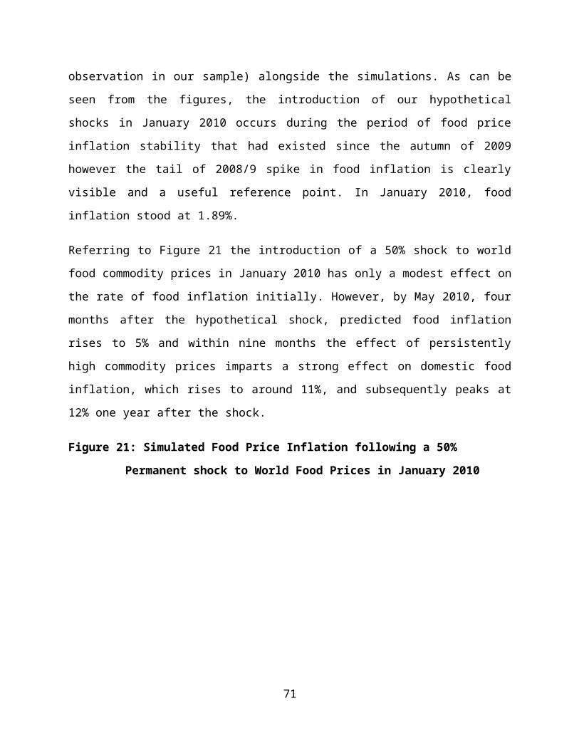
Fruit Price Model

Vegetable Price Model

73

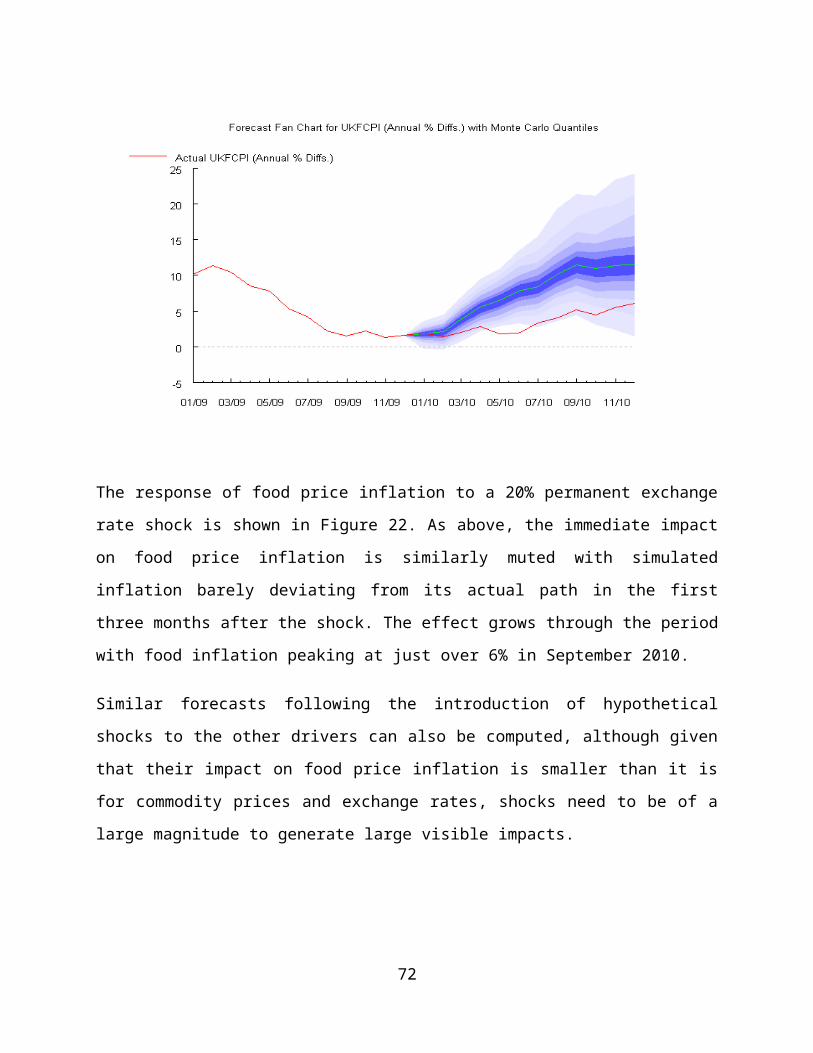
Appendix 5: Data Definitions and Sources

Variable Definition Source NotesUKCPI UK Consumer Price Index (all items). Office for National Statistics (ONS) 2005(M1)=100. Denoted D7BTUKFCPI UK Consumer Food Price Index. OECD, OECD Statistics. http://stats.oecd.org/index.aspx 2005(M1)=100UKRPI UK Retail Price Index (all items). Office for National Statistics (ONS) 2005(M1)=100. Denoted CHAW

WFPI World Food Price Index IMF Primary Commodity Prices: http://www.imf.org/external/np/res/commod/index.asp

Cereals, vegetable oils, protein meals, meats, seafood, sugar, bananas and oranges

ER1 $:£ Exchange rate IMF Financial Statistics 2005(M1)=100

ER2 Monthly average Effective Exchange Rate (Sterling)Bank of England. http://www.bankofengland.co.uk/statistics/index.htm Denoted XUMABK67. Index 2005(1)=100

UKPPI Agricultural Producer price index (UKAPPI). UK DEFRA

Data for 1988(M1)-2009(12) is 2000=100 and was re-based to 2005=100. DEFRA also provide 2005=100 series for 2005(M1)-2010(M1)

Mancost Manufacturing Input costs index. Office for National Statistics (ONS) 2005(M1)=100. Denoted: RNNK.Earn Average Earnings index for the whole economy s.a. Office for National Statistics (ONS) Denoted LMNQ. 2000=100. Re-based to 2005(M1)=100.

Poil Oil Price ; UK Brent, light blend 38 API, fob U.K.IMF Primary Commodity Prices: http://www.imf.org/external/np/res/commod/index.asp $/barrel nominal (needs to be indexed)

U Unemployed: UK (Thousands) s.a. Office for National Statistics (ONS) UK All: Aged 16 - 59/64 in Thousands. Denoted YBSHBCPI CPI for Bread and cereals, Not seasonally adjusted. Office for National Statistics (ONS) 2005(M1)=100. CPI Index 01.1.1. Denoted D7D5MCPI Meat CPI, Not seasonally adjusted. Office for National Statistics (ONS) 2005(M1)=100. CPI Index 01.1.2. Denoted D7D6.FCPI Fruit CPI, Not seasonally adjusted. Office for National Statistics (ONS) 2005(M1)=100. CPI Index 01.1.6. Denoted D7DA

VCPICPI for Vegetables including potatoes and other tuber. n.s.a. Office for National Statistics (ONS) 2005(M1)=100. CPI Index 01.1.7. Denoted D7DB

BAPI UK Producer price index for wheat DEFRA 2005 (M1) =100MAPI UK producer price index for meat DEFRA 2005 (M1) =100FAPI UK producer price index for fruit DEFRA 2005 (M1) =100VAPI UK producer price index for vegetables DEFRA 2005 (M1) =100

74