1

Differences in the Weighting and Choice of Evidence for Plausible versus

Implausible Causes

Kelly M. Goedert

Seton Hall University

Michelle R. Ellefson

University of Cambridge

Bob Rehder

New York University

In Press at JEP: LMC

Author Note

Kelly M. Goedert, Department of Psychology, Seton Hall University; Michelle R.

Ellefson, Faculty of Education, University of Cambridge; Bob Rehder, Department of

Psychology, New York University.

The authors thank Christopher Cagna, Clinton Dudley, Deepak Gera, Mengqi

Guo, Brianna Jozwiak, Klaudia Kosiak, Randall Miller, Robert Rementeria Jr., and

Rebecca Schaffner for their assistance with data collection and data entry.

Correspondence concerning this article should be addressed to Kelly M.

Goedert, Department of Psychology, Seton Hall University, 400 South Orange Ave.,

South Orange, NJ 07079. E-mail: kelly.goedert@shu.edu

2

Abstract

Individuals have difficulty changing their causal beliefs in light of contradictory evidence.

We hypothesized that this difficulty arises because people facing implausible causes

give greater consideration to causal alternatives, which, because of their use of a

positive test strategy, leads to differential weighting of contingency evidence. Across

four experiments, participants learned about plausible or implausible causes of

outcomes. Additionally, we assessed the effects of participants’ ability to think of

alternative causes of the outcomes. Participants either saw complete frequency

information (Exp. 1 and 2), or chose what information to see (Exp. 3 and 4). Consistent

with the positive test account, participants given implausible causes were more likely to

inquire about the occurrence of the outcome in the absence of the cause (Exp. 3 and 4)

than those given plausible causes. Furthermore, they gave less weight to Cells A and B

in a 2 x 2 contingency table and gave either equal or less weight to Cells C and D (Exp.

1 and 2). These effects were inconsistently modified by participants’ ability to consider

alternative causes of the outcome. The total of the observed effects are not predicted by

dominant models of normative causal inference, nor by the particular positive test

account proposed here, but they may be commensurate with a more broadly-construed

positive test account.

3

Differences in the Weighting and Choice of Evidence for Plausible versus

Implausible Causes

Across domains it is commonly observed that prior theories and beliefs influence

how people interpret evidence. For example, individuals have difficulty changing their

causal beliefs in light of contradictory data. This failure to revise beliefs has concerned

experimental psychologists (e.g., Alloy & Tabachnik, 1984; McKenzie & Mikkelsen,

2007; Taylor & Ahn, 2012) and philosophers of science (e.g., Fodor, 1984; Giere, 1994),

with much work addressing its putative normativity. Normative or not, the entrenchment

of prior beliefs is increasingly seen as a problem by science educators, with even the

brightest students holding onto their naïve conceptions about scientific phenomena

(e.g., Chinn & Brewer, 1993; Schauble, 1990; Taber, 2003; Treagust, Chitleborough, &

Mamiala, 2002). Furthermore, it is a problem for society when people maintain

erroneous causal beliefs despite repeated demonstrations to the contrary (e.g., the

belief that vaccines cause autism; Lewandowsky, Ecker, Seifert, Schwarz, & Cook,

2012).

Work on both covariation assessment and on causal inference from contingency

data has demonstrated that judgments about the relation between two events are

biased in the direction of prior expectations (e.g., Billman, Bornstein, & Richards, 1992;

Dennis & Ahn, 2001; Freedman & Smith, 1996; Fugelsang & Thompson, 2000;

Fugelsang & Thompson, 2003; López, Shanks, Almaraz, & Fernández, 1998; Marsh &

Ahn, 2006; Mutter, Strain, & Plumlee, 2007; Schulz, Bonawitz, & Griffiths, 2007; Wright

& Murphy, 1984). For example, after seeing contingency data, people judge two

variables to be more strongly related when they are linked by a plausible causal

4

mechanism (e.g., severed brake lines causing car accidents) rather than an implausible

one (e.g., flat tires causing car start failures; Fugelsang & Thompson, 2000). This effect

obtains not only for beliefs participants have prior to entering the experiment but also

those acquired as part of the experiment (e.g., Garcia-Retamero, Müller, Catena, &

Maldonado, 2009, Exp. 1; Marsh & Ahn, 2006; Taylor & Ahn, 2012). In particular, for

simple causal relations, a primacy effect is observed in the interpretation of contingency

evidence that favors participants’ initial hypotheses (Marsh & Ahn, 2006; Taylor & Ahn,

2012).

How Does Prior Belief Influence Causal Inference from Contingency Evidence?

This paper is primarily concerned with the mechanisms via which prior belief

influences causal inference from contingency data. Prior beliefs take on many forms.

One may have generic knowledge of object kinds, domain-specific knowledge about the

form of relations between causes and outcomes, or prior beliefs about whether the

causal mechanism produces its outcome deterministically versus probabilistically (e.g.,

Cheng, 1997; Griffiths, Sobel, Tenenbaum, & Gopnik, 2011; Lien & Cheng, 2000;

Novick & Cheng, 2004; see Griffiths & Tenenbaum, 2009, for a review). Our interest,

however, is in beliefs concerning the plausibility of specific causal mechanisms.

Some formal theories of rational causal inference are either silent with respect to the

role of specific causal mechanism information (ΔP; Jenkins & Ward, 1965) or

emphasize the importance of purely covariation-based causal learning because it can

occur in the absence of such information (causal power; Cheng, 1997). From a

Bayesian perspective, however, prior beliefs should influence the interpretation of new

evidence (e.g., Koslowski, 1996; McKenzie & Mikkelsen, 2007; Schulz et al., 2007).

5

According to Bayesian inference, current belief in a hypothesis is a product of prior

belief in that hypothesis and the current evidence (Pearl, 2000). Thus, prior beliefs are

expected to affect the interpretation of evidence as part of rational belief updating.

Yet, existing models of Bayesian causal learning (e.g., Griffiths & Tenenbaum, 2005;

Lu, Yuille, Liljeholm, Cheng, & Holyoak, 2008) do not explicitly address how prior

knowledge regarding the believability of a causal mechanism is integrated with

contingency evidence. The closest approximation is a model of causal inference in the

blicket detector paradigm (Griffiths et al., 2011), which accounts for prior knowledge of

the cause’s base rate and whether the causal mechanism is deterministic or

probabilistic. However, this model neither generalizes across domains nor captures the

effects of the believability of the causal mechanism. Variability in the base rate of the

causal objects is not the same as variability in the believability of a causal mechanism:

Infrequently occurring events do not necessarily imply implausible causal mechanisms

(e.g., nuclear fission causing a nuclear explosion). Similarly, both deterministic and

probabilistic relations may vary in their degree of believability.

Fugelsang and Thompson (2003) demonstrated that learners’ prior beliefs indeed

affect how new covariation evidence is interpreted, although the effect varies with the

form of those beliefs. When they established a prior expectation by manipulating the

causal mechanism’s plausibility, participants’ causal judgments varied more with new

contingency evidence for plausible as opposed to implausible mechanisms (see also

Mutter et al., 2007). In contrast, when the expectation took the form of prior covariation

information, participants’ judgments suggested that it was simply added to the new

covariation evidence to form an impression of the strength of the causal relationship.

6

To account for these data, Fugelsang and Thompson introduced a dual process

model of belief-evidence integration, which bears several similarities to the interactional

framework model of Alloy and Tabachnik (1984). This model stipulates that belief-

updating in the face of new covariation evidence occurs in two stages. The first involves

recruiting prior knowledge regarding the relation between the candidate cause and

outcome. This process, which occurs outside of conscious awareness, could yield

knowledge of a causal mechanism and of how the two events covaried in the past. In

the second stage, individuals evaluate new covariation evidence and make an

inference. Fugelsang and Thompson proposed that the weighting of covariation

information increases as a function of the plausibility of the causal mechanism.

A Positive Test Strategy Account of Plausibility Effects on Evidence Weighting

Why is this interaction observed with causal mechanism information? Going a

step beyond Fugelsang and Thompson (2003), we suggest that an implausible

mechanism leads learners to attend to different types of co-occurrence information. This

information—represented by the familiar 2 x 2 table in Figure 1—consists of the number

of cases where the candidate cause and outcome are both present (Cell A), the cause

is present and outcome is absent (B), the cause is absent and the outcome is present

(C), and both are absent (D). We hypothesized that participants faced with plausible

versus implausible causal mechanisms would weight information in these cells

differently.

Research employing cover stories with plausible or neutral causal mechanisms

demonstrates that participants do not weight the four cells equally. When judging the

effects of a putative generative cause participants generally demonstrate the cell-weight

7

inequality A > B ≥ C > D (Mandel & Lehman, 1998). This inequality is observed in

participants' explicit rankings of cell importance (Levin, Wasserman, & Kao, 1993;

Wasserman, Dorner, & Kao, 1990), and in the correlation between participants' causal

judgments and the cell frequencies (Levin et al., 1993; Mandel & Lehman, 1998; Mutter

& Plumlee, 2009). Importantly, this inequality changes for putative preventative causes

such that B is considered the most important cell (B > A > D > C; Mandel & Vartanian,

2009; see also Levin et al., 1993, Exp. 2).

These results have been interpreted as reflecting a positive test strategy (Mandel

& Vartanian, 2009). For generative causes, cells A and B (and especially A) provide

positive tests and cells C and D provide a negative one; for preventative causes, Cell B

provides the most positive test and it becomes more important than A. The primacy

effect observed when contingency information is presented trial-by-trial has also been

interpreted as reflecting a positive test strategy, in which a hypothesis established early

in learning affects the processing of subsequent trials (Marsh & Ahn, 2006). Consistent

with this idea, the interpretation of each cell depends upon participants’ prior learning

experience (Luhmann & Ahn, 2011).

Here, we extend the positive test strategy1 account to the situation of implausible

causes. Whereas Fugelsang and Thompson (2003) suggested that implausible causes

lead learners to place less weight on the data overall, we propose that it also leads to a

shift in cell weights. When faced with a plausible causal mechanism, learners’

preference for few or even single causes (e.g., Dougherty, Gettys, & Thomas, 1997;

Lombrozo, 2007) means they are likely to adopt that plausible cause as their focal

hypothesis, in which case a positive test strategy (Klayman & Ha, 1987; McKenzie,

8

2004) yields the usual cell weight inequality (Levin et al., 1993; Mandel & Lehman,

1998). But when faced with an implausible cause, learners may fail to adopt it as their

focal hypothesis and so the normal overweighting of Cells A and B will be eliminated.

Even further, an implausible cause might encourage a learner to focus on alternative

causes, in which case Cells C and D become the “positive tests.” Cell C may be of

particular importance, because a non-zero frequency in that cell confirms the action of

unobserved alternative causes (e.g., Hagmayer & Waldmann, 2007; Luhmann & Ahn,

2007; Luhmann & Ahn, 2011; Rottman, Ahn, & Luhman, 2011).

Plausibility and the Consideration of Alternative Causes

Although individuals generally prefer few or even single causes of an outcome

(Dougherty et al., 1997; Lombrozo, 2007; Lu et al., 2008; McKenzie, 1994), there are a

number of circumstances in which they do consider causes in addition to those explicitly

presented in an experiment (Cummins, 1995; Fernbach, Darlow, & Sloman, 2010;

Luhmann & Ahn, 2007; see Rottman et al., 2011, for a review). Of particular relevance

here, individuals differ in the number of alternative causes of an outcome they think of

(Dougherty et al., 1997; Hirt & Markman, 1995; Sprenger & Dougherty, 2012). Causal

scenarios also differ, with some supporting more alternative causes than others (e.g.

Cummins, 1995). For example, there are many causes of stress, but few causes of

nuclear explosions. Thus, we hypothesize that the weighting of cause absent

information (e.g., cell C) will increase not only for implausible causes but also as a

function of the number of causes that individuals consider.

9

Predictions of Extant Models

What do extant models predict with regards to the effects of plausibility on data

weighting? Recall that, in contrast to our positive test hypothesis, Fugelsang and

Thompson’s (2003) model of belief-evidence integration predicts that less weight overall

will be given to contingency evidence for implausible causal scenarios. Formal models

of rational causal inference either do not incorporate priors regarding the plausibility of a

specific causal relation (Cheng, 1997; Lu et al., 2008)2 or employ uniform priors

(Griffiths & Tenenbaum, 2005). To determine what these models would predict for

causal relations differing in plausibility, we performed a modeling exercise adding

plausibility-based priors to these models (see Appendix A for a full description of this

exercise). In brief, we employed three different priors to represent differences in the

plausibility of the causal mechanism (.9, .5, and .1 for high, moderate and low

plausibility, respectively). We calculated posterior causal strength as a weighted

average of the prior and the model-specific estimate of causal strength calculated over

randomly-generated 2 x 2 contingency data.3 To calculate cell weights, we regressed

the posterior causal strength estimates on the frequencies for cells A, B, C and D.

Figure 2 excerpts graphs from Appendix A for modified causal power and causal

support when causes are moderately common [p(C) = p(E) = .50], because these best-

illustrate the differing predictions of the two models.

Predictions of the causal strength version of Griffiths and Tenenbaum’s (2005)

causal support model are consistent with that of Fugelsang and Thompson (2003): As

plausibility decreases from .9 to .1, there is decreased weighting of the evidence from

all cells of the contingency table (Figure 2B). In contrast, the modified version of

10

Cheng’s (1997) causal power predicts differential weighting of the cells as a function of

plausibility (Figure 2A): As plausibility decreases from .9 to .1, there is increasing weight

on confirming evidence (Cells A and D) and decreasing weight on disconfirming

evidence (Cells B and C). Thus, in contrast to the positive test hypothesis, the modified

causal power model predicts that evidence disconfirming a prior expectation will be

given more weight.

Finally, while the predictions of the modified causal support and causal power

models were directionally stable across changes in the base rates, predictions of Lu et

al.’s (2008) sparse and strong (SS) priors model varied. With low base rates, those

predictions aligned more with causal power, but with high base rates, they aligned more

with causal support.

In sum, extant models predict either an across the board decrease in cell weights

for implausible causes [Fugelsang & Thompson (2003); our modification of Griffiths &

Tenebaum’s (2005) causal support; and Lu et al.’s (2008) SS priors with high base

rates] or they predict an increase in weighting of confirming evidence, with a decrease

in weighting of disconfirming evidence for implausible causes [modification of causal

power (Cheng, 1997) and Lu et al.’s (2008) SS priors with low base rates]. These

predictions differ from those of the positive test account posed here, which predicts a

decrease in the weighting of cause-present information (Cells A and B) and an increase

in the weighting of cause-absent information (Cells C and D) for implausible causes.

Overview of Current Experiments

Across four experiments we assessed how participants’ use of data varied with the

plausibility of the causal mechanism. Each experiment manipulated the plausibility of

11

causes: participants learned about either highly plausible causal relations (e.g., severed

brakes causing car accidents) or implausible ones (e.g., leather car seats causing car

accidents).

Experiments 1 and 2 tested whether plausibility affects learners’ cell weights. On

each trial, participants received complete frequency information corresponding to the

four cells of the contingency table and made a causal judgment. Experiments 3 and 4

tested whether effects of plausibility extended to participants’ choice of information.

Instead of complete frequency data, they received opportunities to select either a

cause-present case (e.g., car with severed brakes) or a cause-absent case (e.g., car

without severed brakes). Participants then saw the outcome (e.g., whether or not that

car was in an accident). After observing a limited number of cases, participants made

causal judgments. Our primary interest, however, was in participants’ choices. At the

end of Experiments 2 through 4, participants listed as many causes as they could think

of for each of the outcomes.

The positive test strategy account predicts that, relative to those given plausible

causes, participants given implausible causes would place less weight on Cells A and

B, greater weight on Cells C and D, and more frequently choose to inspect cause-

absent cases. Additionally, in Experiments 2 through 4 we tested whether participants’

weighting and choice of evidence varied with their ability to list causal alternatives.

Experiment 1

Method

Participants. Undergraduate students (N = 166; 117 female) attending either

the University of Cambridge or Seton Hall University completed the experiment in partial

12

fulfillment of a course requirement or for ₤10. They ranged in age from 18 to 35 years

(M = 20.12, SD = 2.46).

Procedure. Participants completed the experiment at a computer running E-

Prime 2.0 (Psychology Software Tools, Pittsburgh, PA). All participants learned about

the causes of skin rashes and car accidents in separate randomly-ordered blocks (cover

stories modified from Fugelsang & Thompson, 2000). Different participants received the

plausible and implausible causes (see left half of Table 1). For example, in the plausible

skin rash condition, participants imagined that they were a doctor testing whether hiking

in the woods causes skin rashes. They tested this hypothesis in 16 different doctors’

offices by observing data about whether children went hiking in the woods and whether

they experienced a skin rash. When assessing the causes of car accidents, participants

imagined that they were a police officer investigating whether severed brake lines

(plausible condition) or leather seats (implausible condition) caused car accidents for

cars in 16 different county garages. For both cover stories, participants received

complete frequency data on each of 16 randomly-ordered trials (see rows of Table 2 for

cell frequencies on each trial). For example, on a single trial, some participants saw the

following:

Dr. Gibson's Office

10 children WENT HIKING IN THE WOODS

8 of the 10 developed a skin rash.

5 children DID NOT GO HIKING IN THE WOODS

1 of the 5 developed a skin rash

13

On each trial, participants made a causal judgment between -100 and + 100 (-

100 indicating the cause completely prevents the effect, 0 indicating no effect and +100

indicating the cause completely produces the effect). We instructed participants to base

their judgment on the information from that particular garage (or doctor’s office), and to

disregard other trials.

Design and Data Analysis. We estimated participants’ cell weights by

calculating Pearson correlation coefficients between each participant's judgments

(within cover story) and each of the cell frequencies (i.e., separate correlations for cells

A, B, C, and D). We transformed the correlations into Fisher's z so that they could be

used as measures in the analyses (Mandel & Lehman, 1998; Mandel & Vartanian,

2009). Previous researchers used the absolute value of participants' observed

correlations, changing the sign on the correlations for cells B and C to negative,

because these cells are normatively considered evidence against the hypothesis that

the cause produced the effect (Mandel & Lehman, 1998; Mandel & Vartanian, 2009). In

contrast, we left the sign on participants' observed correlations unaltered when

performing analyses, because participants do not interpret the cell information in the

expected normative way (Luhmann & Ahn, 2011). For ease of interpretation, however,

we present absolute values of the mean cell weights in tables and graphs.

Prior to analysis we screened the data for multivariate outliers based on robust

estimates of Mahalanobis’ distance. The critical value for Mahalanobis’s distance with

two variables and an alpha of 0.05 is 5.992. We calculated separate estimates of

Mahalanobis’s distance for each of the cells. Cases for which Mahalanobis’s distance

exceeded 5.992 for at least one of the cells were counted as outliers and excluded from

14

the analysis. In all experiments, each participant contributed more than one case. Thus,

exclusion of individual cases did not necessarily eliminate whole participants, but we

note when it did. Across experiments, similar patterns of results emerged in the

screened and unscreened data.

We performed 2-level mixed linear model analyses (MLM), with a single random

effect (participants' random intercepts). For the cell weight analyses, we analyzed the

full factorial of the manipulated factors as fixed effects – i.e., 4 (cell: A, B, C, D) x 2

(outcome: skin rashes, car accidents) x 2 (plausibility: plausible, implausible). We

determined the optimal structure for the residual covariance matrix with preliminary

MLM analyses, using likelihood ratio tests to compare models assuming homogeneous

versus heterogeneous variances and covariances, retaining the best-fitting residual

covariance structure. We used maximum likelihood estimation because of our primary

interest in the fixed effects (Singer & Willett, 2003, p.90) and the F distribution with

between-within degrees of freedom (West, Welch, & Galecki, 2007; Rabe-Hesketh &

Skrondal, 2008, p. 111). We followed significant interactions involving the factor of

plausibility with single degree of freedom simple main effects tests (Keppel & Wickens,

2004), testing the effect of plausibility at each level of the variable with which it

interacted. Final covariance structures and results for the random effects are presented

in Appendix B.

Results

Two participants gave causal judgments outside the range of the scale and three

gave judgments of zero on all 32 trials. These five participants were removed prior to

analysis, leaving N = 161. Although the effect of sample did not reach significance, we

15

observed a qualitatively different pattern of cell-weighting among the two samples

(Cambridge/UK vs. Seton Hall/USA). Because the US sample was larger (N = 113; n =

54 for implausible and n = 55 for plausible) and because Experiments 2 through 4

employ US participants, we report the results from the US sample here and report the

results from the smaller UK sample in Appendix C.

Cell Weights. As can be seen in Figure 3, compared to those receiving plausible

causes, implausible participants gave less weight to Cells A and B but similar weight to

C and D. This impression is confirmed by the significant plausibility by cell interaction,

F(3, 761) = 10.45, p < .001. While the implausible group gave less overall weight to the

data than did the plausible group, F(1, 111) = 5.96, p = .016, the difference between the

groups only reached significance for Cells A and B [p < .001, d = 0.57 for Cell A; p

< .001, d = 0.50 for B; p = .523, d = 0.12 for C; p = .081, d = 0.29 for D].

We also observed a main effect of cell, F(3,761) = 10.45, p < .001, whose

interpretation is tempered by the interaction discussed above. No other effects

approached significance [F(3, 761) = 1.66, p = .174, on the plausibility by cell by

outcome interaction; all other Fs < 1].

Discussion

In Experiment 1 we observed that the effect of plausibility differed depending on

the cell. Having an implausible cause lowered participants’ weights for Cells A and B,

relative to having a plausible cause. While directionally this was also true for Cells C

and D, the effect was much smaller and failed to reach significance for these cells.

The results are partially consistent with Fugelsang and Thompson (2003), in that

having an implausible cause lowered reliance on the data. However, the differential

16

weighting of the cells as a function of plausibility is not predicted by Fugelsang and

Thompson (2003), nor by our modification of Griffiths and Tennebaum’s (2005) causal

support (Appendix A), both of which predict lower overall cell weights for the implausible

group. It is also not predicted by the modified causal power model, which predicts an

increase in Cells A and D and a decrease in B and C as the prior probability of the

cause decreases (Appendix A).

The results are partially consistent with our positive test account. We predicted

that relative to plausible participants, those facing implausible causes would give less

weight to Cells A and B and more weight to C and D. Consistent with this hypothesis,

we observed a reduction in the positive test strategy for the experimentally-introduced

causes among the implausible group – as observed in their reduced weights on Cells A

and B. However, we did not observe any evidence that these participants adopted an

alternative focal hypothesis, which we hypothesized would be demonstrated by them

giving more weight to Cell C in particular.

While Experiment 1 yielded partial support for a positive test account, it has

limitations. First, the objective contingencies, which varied between zero and 0.58, were

low and positive; indeed, contingency was zero on half of the 16 trials (Table 2).

Experiment 2 tested a wider range of contingencies.

Second, the standard deviations of the cell frequencies differed (i.e., looking

down the columns in Table 2, SDs ranged from 2.50 to 2.74). Differences in the

variability of cell frequencies might have produced artificial cell weight differences

because higher variability implies a higher maximum correlation with participants’

judgments. Of course, differences in variability cannot explain the differences in cell

17

weights between the plausible and implausible conditions. Nonetheless, in Experiment 2

we equated the cells’ standard deviations.

A third potential limitation was how the frequency information was presented.

Indicating how many times the outcome occurred for the cause present and cause

absent cases gave participants the Cell A and C frequencies but required them to

perform subtraction to determine the frequencies for B and D. For example, participants

told “8 of the 10 children who went hiking in the woods developed a skin rash,” needed

to subtract to determine that 2 of the 10 did not develop a skin rash. Experiment 2

addressed this issue as well.

Experiment 2

Experiment 2 investigated the effects of plausibility and the number of causes

listed on participants’ cell weighting with the aforementioned changes: (a) we explicitly

indicated the numbers corresponding to the frequency in each of the cells (avoiding the

need for subtraction), (b) a broader range of contingencies was tested, and (c) the

standard deviations of the four cells were equated (SDs = 6.68). Because equal

standard deviations entail both positive and negative contingencies, those

contingencies varied between -0.85 and 0.85 (see Table 3).

Experiment 1 tested two outcomes: car accidents and skin rashes. Although

Experiment 1 did not yield outcome effects, to better test for this possibility, and to

extend our results to additional cover stories, we performed pilot testing to identify two

additional outcomes (see Appendix D). The number of causes listed for car accidents

and stress were about the same (M = 7.01, SD = 4.06 and M = 7.07, SD = 3.70,

respectively), as were the number for plant growth and skin rashes (M = 4.33, SD =

18

1.98 and M = 4.04, SD = 2.04). Thus, Experiment 2 tested two outcomes for which

people listed more causes (stress and accidents) and two for which people listed fewer

(plant growth and skin rashes). Finally, at the end of the experiment participants listed

all the possible causes they could think of for these outcomes.

Method

Participants. Seton Hall University undergraduates (N = 125; 86 female)

participated in partial fulfillment of a course requirement (n = 62 implausible and n = 63

plausible). They ranged in age from 18 to 26 years old (M = 18.83, SD = 1.24).

Procedure. The procedure was similar to that of Experiment 1, with a few

exceptions. All participants made causal judgments on 16 trials for each of the four

outcomes in Table 1, for a total of 64 trials. When assessing the causes of plant growth,

participants imagined they were a botanist testing whether fertilizer (plausible) or being

in a blue pot (implausible) led to healthy plant growth for plants in 16 different

greenhouses. When assessing the causes of stress, participants imagined they were a

clinical psychologist testing whether having lots of school deadlines (plausible) or eating

lots of fruits and vegetables (implausible) leads to complaints of stress among students

visiting a school’s counseling center (in 16 different schools).

Order of presentation of the four outcome types was counterbalanced across

participants and trials were presented in a random order. Each row in Table 3

corresponds to one trial and these cell frequencies were explicitly indicated to

participants. For example, on a single trial, a participant may have seen the following:

Dr. Gibson's Office

10 children WENT HIKING IN THE WOODS

19

8 of the 10 developed a skin rash.

2 of the 10 did not develop a skin rash.

5 children DID NOT GO HIKING IN THE WOODS

1 of the 5 developed a skin rash.

4 of the 5 did not develop a skin rash.

After completing all four blocks of trials, participants wrote down all the possible

causes they could think of for each of the four outcomes (order counter-balanced across

participants). In all other respects, the procedure for Experiment 2 was that same as

that for Experiment 1.

Design and Data Analysis. We calculated cell weights and performed MLM

analyses as in Experiment 1, analyzing the full factorial of the manipulated variables

and the number of listed alternatives as fixed factors in the MLM – i.e., a 4 (outcome:

skin rashes, accidents, plant growth, stress) x 2 (plausibility: implausible, plausible) x 4

(cell: A, B, C, D) x number of listed alternatives.

In this and subsequent experiments we observed that the range on the number

listed alternatives often differed for the implausible and plausible groups. Because a

difference in range could alter the size of the coefficient for predicting cell weights, we

performed the analysis over the smaller range of cases. Prior to analyses we screened

for outliers as in Experiment 1.

Results

One participant from the implausible condition was excluded from the analysis for

giving causal judgments of zero on all 64 trials, leaving N = 124 (n = 61 and 63 in

implausible and plausible, respectively).

20

Number of Causes Listed. While one might suspect that participants given

implausible causes would be induced to think of more alternatives, participants in the

implausible (M = 6.74, SD = 3.77) and plausible (M = 6.89, SD = 3.81) conditions listed

a similar number of alternatives, F < 1, an effect replicating Fugelsang and Thompson

(2000, Exp. 3). However, the number of alternatives listed varied by outcome, F(3, 496)

= 33.17, p < .001. Consistent with the pilot study, participants listed more causes for car

accidents (M = 8.23, SD = 3.87) and stress (M = 8.68, SD = 4.69) than for skin rashes

(M = 5.27, SD = 2.53) and plant growth [M = 5.09, SD = 1.82; ps < .001 for Bonferroni

comparisons]. Car accidents and stress did not differ from each other (p = .893), nor

did skin rashes and plant growth (p = 1.00). Outcome and plausibility did not interact, F

< 1.

Cell Weights. There were no outliers, but the range of listed alternatives was

smaller for the implausible (2, 26) than the plausible (1, 26) group. We analyzed cases

falling within the smaller range.

As seen in Figure 4, implausible and plausible participants differently weighted

the frequency data from the cells [F(3, 1742) = 8.19, p < .001 for plausibility by cell

interaction]. However, unlike Experiment 1, implausible participants gave significantly

less weight to all cells than did plausible participants [p < .001, d = 0.48 for Cell A; p

= .032, d = 0.21 for Cell B; p < .001, d = 0.45 for Cell C; and p = .021, d = 0.21 for Cell

D]. The interaction obtained because while implausible participants gave similar weight

to all four cells, F(3,1741) = 1.49, p = .215, cell weights for plausible participants varied,

F(3, 1742) = 19.04, p < .001. They gave more weight to Cell A than B, p < .001, d =

0.56, and more weight to C than D, p < .001, d = 0.44, while the weights for A and C

21

and that for B and D did not differ (p = .117, d = 0.13 and p = .975, d = 0.03,

respectively).

As seen in Table 4, the slopes for predicting cell weights from the number of

listed alternatives varied across cells [F(3, 1742) = 2.66, p = 0.047, for the cell by listed

alternatives interaction]. Collapsed across plausibility conditions, as participants listed

more alternatives, they placed greater negative weight on disconfirming evidence – i.e.,

frequency information from Cells B and C (Figure 5). This effect reached significance for

Cell B, p = .032, but not for Cell C, p = .061.

We also observed significant main effects of plausibility, F(1, 1742) = 14.22, p

< .001 and listed alternatives, F(1, 1742) = 3.85, p = .050, whose interpretations are

tempered by the interactions described above. No other effects approached

significance, ps > .11.

Discussion

In Experiment 2, implausible participants gave less weight to the data than did

plausible participants. This result is consistent with the predictions of Fugelsang and

Thompson (2003) and of the modified causal support model (Appendix A and Figure

2b). Additionally, we observed that all participants placed greater weight on

disconfirming evidence as they listed more alternative causes. This result is consistent

with studies finding that individuals generating more alternative causes judge a focal

cause to be less likely compared to individuals generating fewer alternatives (Dougherty

et al., 1997; Hirt & Markman, 1995). It is also consistent with a positive test strategy,

broadly construed. Our version of the positive test account posited that participants

facing implausible causes – or who think of many alternatives – may not only fail to

22

adopt the experimentally-presented putative cause as their focal hypothesis, but may

instead adopt an alternative cause as their focal hypothesis. The results of Experiments

1 and 2 do not support the latter prediction. However, we did observe support for a

broadly construed version of the positive test account in which implausibility – or

thinking of many alternatives – reduces the positive test for the experimentally-

presented cause. In both experiments there was a reduction in the weighting of cause-

present information for implausible causes, and in Experiment 2 participants thinking of

more alternatives gave more weight to evidence disconfirming the experimentally-

presented focal cause.

Experiments 1 and 2 differed in how implausible participants weighted Cells C

and D (relative to plausible participants). This difference cannot be attributed to the new

cover stories, because an analysis of only the two outcomes used in Experiment 1 left

the results of Experiment 2 qualitatively unchanged. While we do not have a definitive

account for why these experiments differed, the common finding across both

experiments – a reduction in the weighting of data from Cells A and B – is predicted by

both the positive test account and Fugelsang and Thompson’s (2003) dual process

model. We next tested whether this effect generalized to an information search

paradigm.

Overview of Experiments 3 and 4

Experiments 3 and 4 assessed whether the effects of plausibility extended to

participants’ choices about what information they would like to see. While in

Experiments 1 and 2 participants received complete contingency information on every

trial, in Experiments 3 and 4 they saw a limited number of cases. On each trial,

23

participants elected to see a case where the cause was either present or absent, after

which they learned that case’s outcome. Participants chose five and nine cases to

observe in Experiments 3 and 4, respectively. We expected a positive test bias (more

“cause-present” cases chosen overall), but also an effect of plausibility such that

participants given implausible causes would select fewer cause-present cases. We also

expected that participants’ choice of cause-present cases may vary with the number of

listed alternatives.

Experiment 3

Method

Participants. Seton Hall University undergraduates (N = 109; 74 female)

participated in partial fulfillment of a course requirement (n = 55 plausible; n = 54

implausible). They ranged in age from 18 to 41 years old (M = 19.70, SD = 3.08).

Procedure. Participants learned of the causes of car accidents and skin rashes,

with plausibility of the causes manipulated between-groups (as in Experiment 1). In

contrast to previous experiments, there were only four trials, over which participants

learned about four different doctor's offices (or county garages). For each office,

participants read that there were 12 patients, six representing cause-present cases and

six cause-absent cases. However, participants could view the files of only five of these

12 patients. Each sub-trial consisted of participants making a single choice to either

view a file in which the cause was present or one in which it was absent. Figure 6A

depicts a choice screen representing a sub-trial for participants in the plausible skin

rash condition.

24

The presentation order of the cause-present and cause-absent choices was

counter-balanced between participants: Half pressed 1 to see a cause present case (as

depicted in 6A) and half pressed 2, in which case the cause-present option appeared in

the second position. After making their choice, participants saw a screen indicating the

choice they made and the outcome (see Figure 6B). This screen remained visible until

participants pressed the space bar, ending the sub-trial. After making five selections,

participants made causal judgments on the same scale as in Experiment 1. Prior to

beginning the experiment, participants received booklets to record both their choices

and the outcome, so that they would not have to rely upon their memory when making

causal judgments. After the choice and causal judgment task, participants listed all

possible causes they could think of for car accidents and skin rashes (order

counterbalanced across participants).

The objective contingency across all 12 files (of which participants only saw five)

was zero. Each trial was associated with separate matrices for the cause-present and

cause-absent choices. Within each matrix, three of the files indicated a presence of the

outcome and three did not. For any given sub-trial, an outcome was chosen from the

appropriate matrix (depending on the participant's choice) at random, without

replacement. Thus, while the objective contingency was zero, each participant observed

a different objective contingency based on that participant's choices and the random

selection of the outcome.

Design and Data Analysis. We cleaned the data by eliminating individual sub-

trials for which the participant’s response time was less than 250ms (5% of sub-trials).

We then obtained the percent of cause present choices for each trial and took the

25

average of that across each participant’s four trials. The design of the experiment was

a 2 (outcome: skin rashes, accidents) x 2 (plausibility: implausible, plausible) x 2 (option

order: cause present first, cause present second) mixed design with outcome

manipulated within-groups and plausibility and option order between-groups. We

performed 2-level MLM analyses as in Experiments 1 and 2.

Results and Discussion

We excluded two participants because they failed to make any causal judgments.

An additional three participants failed to list causes at the end of the experiment, leaving

N = 104 (n = 50 plausible; n = 54 implausible).

Number of Causes Listed. Consistent with Experiment 2, participants in the

implausible (M = 7.62, SD = 4.32) and plausible conditions (M = 7.00, SD = 2.88) listed

a similar number of causes [F(1,102) = 2.90, p = .091, d = 0.17], but they listed more

causes of car accidents (M = 8.84, SD = 4.05) than of skin rashes [M = 5.79, SD = 2.54;

F(1, 206) = 41.23, p < .001, d = 0.82]. The plausibility by outcome interaction did not

reach significance, F < 1.

Information Choice. Because we observed different ranges for the number of

listed alternatives in the plausible (2, 14) and implausible (0, 26) conditions, we

restricted the analysis to cases falling in the smaller range. No cases were identified as

multivariate outliers.

Overall, we observed a small positive test bias: On average, participants chose

the cause-present option more frequently than expected by chance (M = .528, SD =

0.10; one-sample t versus .50: t(103) = 2.04, p = .044, d = 0.24). Consistent with our

expectation, this positive test bias was smaller among implausible participants: They

26

made fewer cause-present choices (M = .517, SD = .10) than did plausible participants

[M = .539, SD = .11; F(1, 100) = 5.16, p = .025, d = 0.15, for the main effect of

plausibility]. We also observed an interaction between plausibility and the number of

listed alternatives, F(1, 91) = 6.70, p = .011, which is depicted in Figure 7. Relative to

the plausible condition, as participants in the implausible condition listed more causes,

they chose the cause-present option less often (comparing slopes to zero: b = -0.007,

SE = .005, β = -0.17, p = .162 for implausible; b = 0.004, SE = .005, β = 0.07, p = .424

for plausible).

While no other effects reached significance, ps ≥.06, there was a tendency for

participants to choose the cause present option more often when that option appeared

first (M = .57, SD = .11) versus second (M = .47 , SD = .14), F(1,100) = 3.68, p = .058.

Discussion

Relative to the plausible group, implausible participants chose the cause-present

option less often and their cause-present choices decreased as they listed more causes

of the outcomes. Although both of these effects were small (d = 0.15 for the effect of

plausibility; β = -0.17 for the implausible group’s slope), they are uniquely predicted by a

positive test account.

Experiment 4

The goal of Experiment 4 was to address limitations of Experiment 3, some of

which may have led to its small effects. First, because the potential effect of option

order may have obscured the strength of the plausibility effect, we modified the way in

which participants made their choices. Instead of pressing number keys mapped to the

top and bottom choices, they used the mouse to click a box on the left or right of the

27

computer screen (see Figure 8). Second, because Experiment 3 participants observed

only five cases before making a causal judgment, it is likely that they did not see all four

cells of the contingency table on many trials. Experiment 4 participants made nine

choices and so observed nine cases on every trial. This adjustment not only gave them

more information, it allowed us to calculate cell weights. Third, Experiment 4 tested the

four outcomes used in Experiment 2.

A final change was to the data from which participants selected cases.

Experiment 3’s cases were drawn from matrices with an equal number of cause-present

and cause-absent cases and objective contingencies of zero (if participants had seen

complete information). Experiment 4’s cases were drawn from matrices based on the

cell frequencies of a subset of the trials used in Experiment 2 (Table 3).

Method

Participants. Seton Hall University undergraduates (N = 105; 60 female)

participated in partial fulfillment of a course requirement (n = 52 implausible; n = 53

plausible). They ranged in age from 18 to 26 years old (M = 18.96, SD = 1.25).

Procedure. The procedure was very similar to that of Experiment 3 but

employed the four outcomes used in Experiment 2 (car accidents, skin rash, stress and

plant growth). Like Experiment 3, over four trials participants learned about four different

doctor's offices (or county garages, or greenhouses, or counseling offices). Each of

these four “offices” corresponded to one of the bottom four rows of Table 3. Participants

were told the total number of cause-present and cause-absent cases and were allowed

to make nine choices on each trial. Participants made their choice by clicking a box to

the left or right on the computer screen (Figure 8). The order of the cause-present and

28

cause-absent choices was counter-balanced between participants: Half clicked the box

on the left to make their cause-present choice and half the one on the right. Participants

received feedback regarding the outcome based on their choice (as in Figure 6b).

Feedback was determined by randomly drawing without replacement from matrices

constructed to match the bottom four rows of Table 3. The feedback screen remained

visible until participants pressed the space bar, ending the sub-trial. After making nine

selections, participants made causal judgments as in previous experiments. Like

Experiment 3, participants received booklets in which they recorded their choices and

the outcomes. After completing the choice task, they listed all the possible causes they

could think of for all the outcomes (order counterbalanced across participants).

Design and Data Analysis. We cleaned the data by eliminating individual sub-

trials for which a participant’s response time was less than 250ms (4.9% of sub-trials).

We then computed the percent of cause-present choices for each trial and took the

average of the participant's four trials as the primary dependent measure. The design of

the experiment was a 4 (outcome: skin rashes, accidents, plant growth, stress) x 2

(plausibility: implausible, plausible) x 2 (option order: cause present left, cause present

right) mixed design with outcome manipulated within-groups and plausibility and option

order between-groups. We again performed 2-level MLM analyses.

Although our primary dependent measure for Experiment 4 was the proportion of

cause present choices, because participants saw nine cases for each trial, we also

calculated cell weights as in Experiments 1 and 2. Note that because the exact cell

information participants received depended both on their choices and on the random

29

draw from the frequency table, each participant observed different frequencies in each

of the cells (and hence different objective contingencies).

Results

We excluded two participants because they gave causal judgments outside the

range of the scale, leaving N = 103 (n = 52 implausible; n = 51 plausible).

Number of Causes Listed. As in the previous experiments, participants in the

plausible (M = 5.68, SD = 3.14) and implausible (M = 6.21, SD = 3.29) conditions listed

similar numbers of causes, F < 1, but the number of causes they listed varied with the

outcome, F(3, 297) = 30.01, p < .001. While participants listed a similar number for car

accidents (M = 7.26, SD = 3.45) and stress (M = 7.02, SD = 3.79), p = 1.00, and for

plant growth (M = 4.94, SD = 2.05) and skin rashes (M = 4.55, SD = 2.36), p = .171, all

other pairwise comparisons among the outcomes reached significance, ps < .001. The

plausibility by outcome interaction did not reach significance, F(3, 297) = 1.22, p = .303.

Information Choice. We observed different ranges in the listed alternatives for

the plausible (0, 27) and implausible (0, 21) groups and thus, restricted the analysis to

the smaller range of alternatives. There were 8 multivariate outliers. While the exclusion

of individual cases does not necessarily involve excluding whole participants, doing so

led to the exclusion of two participants in the plausible condition, leaving N = 101 for the

choice data (n = 52 implausible; n = 49 plausible).

Consistent with Experiment 3, we observed an overall positive test bias:

Participants chose the cause-present option more often than expected by chance (M

= .554, SD = .13, one-sample t versus .50: t(100) = 4.11, p < .001, d = 0.41). The main

effect of plausibility was the only effect to approach significance, F(1,97) = 3.32, p

30

= .075, d = .19, reflecting a tendency for implausible participants to make fewer cause

present choices (M = .544, SD = .12) than plausible participants (M = .569, SD = .15).

While this effect failed to reach significance, the size of the plausibility effect here (d =

0.19) was larger than the significant effect in Experiment 3 (d = 0.15). This difference

may result from a slightly higher standard error on the effect of plausibility in Experiment

4 (SE = .087) relative to Experiment 3 (SE = .069); the significant plausibility by number

of listed alternatives interaction in Experiment 3 likely reduced the error variance in that

experiment. In Experiment 4, we did not observe an interaction between plausibility and

the number of listed alternatives, F < 1. Nor did the number of listed alternatives

independently predict the proportion of cause-present choices, F < 1. Finally, none of

the effects involving option ordering approached significance (ps > .31), which suggests

that the new procedure for making selections successfully eliminated the tendency for

option ordering to affect the choice data.

Cell Weights. As described for the choice data, we restricted the analysis to the

smaller range of alternatives. Four cases were excluded as multivariate outliers.

Furthermore, one participant in the implausible condition gave causal judgments of zero

on all trials, rendering it impossible to calculate the participant’s cell weights. These

exclusions left N = 98 for the cell weight analysis (n = 50 implausible; n = 48 plausible).

As seen in Figure 9, we observed differential weighting of the cells as a function

of plausibility [F(3, 1099) = 4.81, p = .002, for the cell by plausibility interaction].

Replicating Experiment 1, implausible participants gave less weight to Cells A and B

than did plausible participants [F(1, 1099) = 5.42, p = .020, d = 0.19, collapsing across

31

the absolute value of the means on A and B], but the groups weighted C and D similarly

[F < 1, collapsing across the absolute value of the means on C and D].

The differential cell weighting among the groups was further modified by the

number of listed alternatives [F(3, 1099) = 3.81, p = .009, for the three-way interaction].

Marginal slopes for this interaction appear in Table 5. Differences between the slopes of

the plausible and implausible groups reached significance only for Cell A. Comparing

the slopes to zero, implausible participants placed more positive weight on Cell A and

more negative weight on Cell B as they listed more alternatives (see Figure 10).

No other effects reached significance [p = .071 for the main effect of cell; p

= .059 for the plausibility by listed alternatives interaction; and all other ps ≥ .20].

Discussion

Participants in the implausible condition of Experiment 4 tended to choose the

cause-present option less often than those in the plausible condition (d = 0.19). They

also placed less weight on Cells A and B (d = 0.19) and similar weight on C and D. This

pattern of weighting and choice is consistent with that observed in the earlier

experiments. However, the modifying effect of the number of listed alternatives was not

consistent with prior experiments: Participants in the implausible group of Experiment 4

placed more weight on Cells A and B as they listed more alternatives. This effect is also

not consistent with predictions of the extant models, nor with a positive test account.

General Discussion

Our experiments addressed two questions: 1) Do participants use data differently

when faced with plausible versus implausible causal mechanisms? and 2) Are effects of

32

plausibility moderated by consideration of alternative causes? Our results suggest that

the answer to the first question is “yes,” while that for the second is more equivocal.

Does Plausibility Differentially Affect Data Use?

Yes. Across experiments, we found that participants facing implausible causes

gave less weight to cells A and B than did those facing plausible causes. This effect of

plausibility extended to participants’ choices: Relative to plausible participants,

implausible participants more frequently chose cause-absent over cause-present data

(Experiments 3 and 4). These results are consistent with the positive test hypothesis.

However, the effect of plausibility on the weighting of cells C and D was less

clear. We predicted that participants faced with an implausible cause may adopt an

alternative focal hypothesis, leading them to place more weight on Cells C and D

(relative to the plausible participants). We did not observe this predicted pattern (but see

Appendix C). In contrast to our hypothesis, implausible participants either placed less

weight (Experiment 2), or similar weight (Experiments 1 and 4) on cells C and D relative

to plausible participants. Thus, while the reduction of the Cell A and B weights for the

implausible group was consistent with the positive test account, we did not observe

evidence that these participants selected an alternative focal hypothesis, as

represented by frequency information in Cells C and D.

Moderating Effect of Considering Alternative Causes?

We observed moderating effects of the number of alternative causes participants

listed on both cell weights and on information choice. However, these effects were not

consistent across experiments. In Experiment 2, participants in both plausible and

implausible conditions placed more weight on disconfirming evidence (Cells B and C) as

33

they listed more alternative causes. In Experiment 3, participants in the implausible

condition chose to see more cause-absent information as they listed more alternative

causes. Both of these effects may be consistent with a broadly construed positive test

account. As individuals think of more alternatives, they place less weight on positive test

evidence for the experimentally-introduced cause. However, in Experiment 4, the

number of listed alternatives failed to predict the choice data, and in the cell weight data

implausible participants placed more weight on Cells A and B as they listed more

causes.

Why did we observe these inconsistent results across experiments? It is possible

that these inconsistencies resulted from limitations in our method for assessing the

consideration of alternative causes: We relied on participants’ listing of causes at the

end of the experiment to make inferences about what participants were considering

during the experiment. Because we collected information on the number of alternative

causes after-the-fact, and because this information reflects an individual difference

rather than a manipulated difference, we are left with the possibility that the listing of

alternative causes and causal judgments are related because of an additional variable

that we did not assess. A more stringent test of our hypothesis would involve creating

fake causal worlds in which the objective number of alternative causes supported by

events is manipulated.4

Indeed, we postulated that differences in the ability to think of alternatives may

stem not only from individual differences (i.e., overall, some people think of more

causes than do others; Dougherty et al., 1997; Sprenger & Dougherty, 2012), but also

from differences in the causal scenarios themselves (Cummins, 1995). That is, some

34

outcomes support more causes than others (e.g., the number of causes of a nuclear

explosion versus the number of causes of stress). We observed such a difference here:

Across experiments, participants consistently listed more causes of car accidents and

stress than of skin rashes and plant growth. Why did we fail to observe effects of the

outcomes employed in the causal scenarios? One possibility is that because of shared

variance it is not possible to observe effects of the number of alternatives outcomes

support when the number of alternatives participants can list is already entered in an

analysis.4 An additional possibility is that manipulation of the number of alternatives

supported by the outcomes was not robust enough. In Experiments 2 and 4, the

outcomes that supported “more” versus “fewer” alternatives, while statistically different

from each other, differed by an average of only two to three causes. While our pilot

testing also identified two kinds of events for which people could list even fewer

alternatives (colon cancer and chemical reactions; see Appendix D), our more pressing

interest was in investigating the moderating effects of individual differences in the

consideration of causal alternatives on plausibility. Thus, we avoided choosing

outcomes that were at the low extreme in terms of the number of causes they

supported, for which participants might be at floor when listing alternatives. Future work

will need to more systematically address how the ability of outcomes to support more

versus fewer causes affects evidence weighting.

In sum, we may have observed inconsistent moderating effects of the

consideration of alternative causes because of limitations of the method we employed

for its measurement. Future work correcting for some of these limitations is necessary

35

to clarify exactly how the consideration of alternative causes affects the choice and

weighting of data.

Implications for Theories of Causal Inference from Data

The effects of plausibility observed in the current set of experiments were clearly

inconsistent with our modification of Cheng’s (1997) causal power (Figure 2a and

Appendix A). That model predicts decreases in plausibility associated with increasing

weight on Cells A and D (confirming information) and decreasing weights on Cells B

and C (disconfirming information). In contrast, we observed decreases in plausibility to

be associated with decreasing weights on Cells A and B, and either similar

(Experiments 1 and 4) or decreased weights on Cells C and D (Experiment 2).

Both Fugelsang and Thompson (2003) and the modification of Griffiths and

Tenenbaum’s (2005) causal support (Figure 2b and Appendix A) predict a reduction in

the weighting of the data from all cells. The consistent observation across experiments

that implausible participants gave less weight to Cells A and B is partially

commensurate with these accounts. However, across experiments we observed

differential weighting of the cell frequency data among plausible and implausible

participants not predicted by these accounts. In Experiments 1 and 4, implausible

participants gave less weight to Cells A and B, and similar weight to cells C and D

relative to plausible participants. In Experiment 2, while implausible participants gave

less weight to all cells than did plausible participants, they gave equal weight to the

cells, and plausible participants weighted A > B and C > D (Figure 4).

Given that Fugelsang and Thompson (2003) and the modified causal support

predict that implausibility leads to an across the board reduction in cell weights (with no

36

differential weighting patterns for plausible and implausible causes), our results are

inconsistent with those predictions. Rather, our results may be consistent with a more

broadly construed positive test strategy account – one in which implausibility functions

primarily to reduce the positive test of the experimentally-presented cause (i.e., reduce

the weighting of cause-present information).

An additional consideration not explicitly addressed by most extant formal models

of causal learning, nor by our experiments, is the relatively rarity of the events involved

(cf. Hattori & Oaksford, 2007). Heavy weighting of Cell A information depends on the

assumption that the presence of events is rare, while their absence is quite common.

Given rare events, Cell A better-discriminates between two causal alternatives than

does Cell D (Anderson, 1990; McKenzie, 2004; McKenzie & Mikkelsen, 2007).

Consistent with this argument, participants place more weight on Cell D information for

events whose absence is rare (McKenzie & Mikkelsen, 2007). Our modeling exercise

(Appendix A) also supports the importance of the rarity assumption. When we gave the

models data generated by randomly sampling values for the frequencies in the each of

the four cells [p(C) ≈ p(E) ≈ .50], the models did not predict the cell-weight inequality

typically observed for generative causes. However, when we introduced a rarity bias on

the presence of events into the data-generation process the model predictions

approximated the cell-weight inequality and when the presence of events was common,

the models predicted heavy weighting of Cell D information (Appendix A). Across our

Experiments 1 and 2, the causes and outcomes were moderately frequent [p(C) = p(E)

= .48 in Experiment 1 and p(C) = p(E) = .50 in Experiment 2]. Thus, differences in the

relative rarity of the causes and outcomes cannot explain any of the data-weighting

37

differences we observed for Cells C and D across those experiments. Nonetheless, a

complete theory of evidence weighting will need to account for plausibility, the

consideration of alternative causes, and for the effects of the relative rarity of the causes

and their outcomes.

As a final point, our results have implications for researchers testing hypotheses

about causal reasoning from covariation data. Participants may use this data differently

with different causal scenarios affording the consideration of more or fewer alternatives.

Additionally, our data suggest that the results of laboratory experiments using fabricated

causes and outcomes (of which participants have no prior knowledge), may not

generalize well to situations in which individuals make causal inferences regarding

events for which they have prior beliefs (see also Cummins, 1995).

Conclusion

Across experiments we observed that participants use and weighting of data

varied with the plausibility of a cause’s mechanism in a manner partially consistent with

Fugelsang and Thompson’s (2003) dual process model and partially consistent with a

broadly-construed positive test account. While these effects were further modified by

participants’ ability to consider alternative causes of the outcome, the manner in which

they were modified varied across experiments. Additional factors may also influence

participants’ cell weights. Determination of precisely how these factors interact with

plausibility and consideration of alternatives awaits future systematic investigation.

38

Footnotes

1 We refrained from using the phrase confirmation bias for two reasons: 1) Confirmation

bias does not necessarily result from a positive test strategy. Rather, confirmation bias

results from a combination of factors at both test and evaluation stages of hypothesis

testing (Klayman, 1995; McKenzie, 2004; Slowiaczek, Klayman, Sherman, & Skov,

1992). 2) The phrase confirmation bias implies non-normativity, but the relative non-

normativity of seeking confirming evidence is disputed: Under certain conditions seeking

confirmation may be normative (e.g., Austerweil & Griffiths, 2011).

2 In their Appendix C, Lu et al. (2008) introduce a specific prior of zero on the strength of

background causes in the blicket detector paradigm, because participants learn that

only blickets and no other objects activate the blicket detector. Although they have

modeled a specific prior, this prior is on the strength of the background causes rather

than on the believability of the focal cause.

3 Taking a weighted average of the prior does not capture previous findings that prior

causal mechanism information interacts with new contingency evidence (Fugelsang &

Thompson, 2003). However, the weighted average reflects a Bayesian belief updating.

4 However, an additional observation suggests that we are both tapping the

consideration of alternative causes and that the number of alternatives supported by

different outcomes may be important: For all experiments we performed preliminary

analyses investigating the effects of plausibility on cells weights and information choice

excluding the number of listed alternatives – i.e., without the moderator. In Experiment

2, we observed an effect of outcome type in these analyses: Participants’ cell weights

varied with the outcome [cell by outcome interaction, F(3, 842) = 3.93, p = .008].

39

Overall, participants placed less weight on the data when the outcomes supported more

(car accidents and stress) versus fewer alternatives (skin rash and plant growth), with

this effect reaching significance for Cells B and D (ps < .04). This effect of outcome type

disappeared once the number of alternatives listed at the end of the experiment was

added to the model, consistent with the assumption that differences between the

outcomes were driven by the number of alternative causes those outcomes supported.

40

References

Alloy, L. B., & Tabachnik, N. (1984). Assessment of covariation by humans and animals:

The joint influence of prior expectations and current situational information.

Psychological Review, 91(1), 112-149. doi:10.1037/0033-295X.91.1.112

Anderson, J. R. (1990). The adaptive character of thought. Hillsdale, NJ England:

Lawrence Erlbaum Associates, Inc.

Billman, D., Bornstein, B., & Richards, J. (1992). Effects of expectancy on assessing

covariation in data: 'Prior belief' versus 'meaning.'. Organizational Behavior and

Human Decision Processes, 53(1), 74-88. doi:10.1016/0749-5978(92)90055-C

Cheng, P. W. (1997). From covariation to causation: A causal power theory.

Psychological Review, 104(2), 367-405. doi:10.1037/0033-295X.104.2.367

Chinn, C. A., & Brewer, W. F. (1993). The role of anomalous data in knowledge

acquisition: A theoretical framework and implications for science instruction. Review

of Educational Research, 63, 1-49. doi: 10.2307/1170558

Cummins, D. D. (1995). Naive theories and causal deduction. Memory & Cognition,

23(5), 646-658. doi:10.3758/BF03197265

Dennis, M. J., & Ahn, W. (2001). Primacy in causal strength judgments: The effect of

initial evidence for generative versus inhibitory relationships. Memory & Cognition,

29(1), 152-164. doi:10.3758/BF03195749

Dougherty, M. R. P., Gettys, C. F., & Thomas, R. P. (1997). The role of mental

simulation in judgments of likelihood. Organizational Behavior and Human Decision

Processes, 70(2), 135-148. doi:10.1006/obhd.1997.2700

41

Fernbach, P. M., Darlow, A., & Sloman, S. A. (2010). Neglect of alternative causes in

predictive but not diagnostic reasoning. Psychological Science, 21(3), 329-336.

doi:10.1177/0956797610361430

Fodor, J. A. (1984). Observation reconsidered. Philosophy of Science, 51, 23-43.

Freedman, E. G., & Smith, L. D. (1996). The role of data and theory in covariation

assessment: Implications for the theory-ladenness of observation. Journal of Mind

and Behavior, 17(4), 321-343.

Fugelsang, J. A., & Thompson, V. A. (2000). Strategy selection in causal reasoning:

When beliefs and covariation collide. Canadian Journal of Experimental

Psychology, 54(1), 15-32.

Fugelsang, J. A., & Thompson, V. A. (2003). A dual-process model of belief and

evidence interactions in causal reasoning. Memory & Cognition, 31(5), 800-815.

Garcia-Retamero, R., Müller, S. M., Catena, A., & Maldonado, A. (2009). The power of

causal beliefs and conflicting evidence on causal judgments and decision making.

Learning and Motivation, 40(3), 284-297. doi:10.1016/j.lmot.2009.04.001

Giere, R. N. (1994). The cognitive structure of scientific theories. Philosophy of Science,

61, 276-296.

Griffiths, T. L., Sobel, D. M., Tenenbaum, J. B., & Gopnik, A. (2011). Bayes and

blickets: Effects of knowledge on causal induction in children and adults. Cognitive

Science, 35(8), 1407-1455. doi:10.1111/j.1551-6709.2011.01203.x

Griffiths, T. L., & Tenenbaum, J. B. (2005). Structure and strength in causal induction.

Cognitive Psychology, 51(4), 334-384. doi:10.1016/j.cogpsych.2005.05.004

42

Griffiths, T. L., & Tenenbaum, J. B. (2009). Theory-based causal induction.

Psychological Review, 116(4), 661-716. doi:10.1037/a0017201

Hagmayer, Y., & Waldmann, M. R. (2007). Inferences about unobserved causes in

human contingency learning. The Quarterly Journal of Experimental Psychology,

60(3), 330-355. doi:10.1080/17470210601002470

Hattori, M., & Oaksford, M. (2007). Adaptive non-interventional heuristics for covariation

detection in causal induction: Model comparison and rational analysis. Cognitive

Science: A Multidisciplinary Journal, 31(5), 765-814.

doi:10.1080/03640210701530755

Hirt, E. R., & Markman, K. D. (1995). Multiple explanation: A consider-an-alternative

strategy for debiasing judgments. Journal of Personality and Social Psychology,

69(6), 1069-1086. doi:10.1037/0022-3514.69.6.1069

Jenkins, H. M., & Ward, W. C. (1965). Judgment of contingency between responses

and outcomes. Psychological Monographs: General and Applied, 79(1), 1-17.

doi:10.1037/h0093874

Keppel, G., & Wickens, C. D. (2004). Design and analysis: A researcher's handbook

(4th ed.). Upper Saddle River, NJ: Prentice Hall.

Klayman, J. (1995). Varieties of confirmation bias. Psychology of Learning and

Motivation, 32, 385-418.

Klayman, J., & Ha, Y. (1987). Confirmation, disconfirmation, and information in

hypothesis testing. Psychological Review, 94(2), 211-228. doi:10.1037/0033-

295X.94.2.211

43

Koslowski, B. (1996). Theory and evidence: The development of scientific reasoning.

Cambridge, MA US: The MIT Press.

Levin, I. P., Wasserman, E. A., & Kao, S. (1993). Multiple methods for examining biased

information use in contingency judgments. Organizational Behavior and Human

Decision Processes, 55(2), 228-250. doi:10.1006/obhd.1993.1032

Lewandowsky, S., Ecker, U. K. H., Seifert, C. M., Schwarz, N., & Cook, J. (2012).

Misinformation and its correction: Continued influence and successful debiasing.

Psychological Science in the Public Interest, 13(3), 106-131.

doi:10.1177/1529100612451018

Lien, Y., & Cheng, P. W. (2000). Distinguishing genuine from spurious causes: A

coherence hypothesis. Cognitive Psychology, 40(2), 87-137.

doi:10.1006/cogp.1999.0724

Lombrozo, T. (2007). Simplicity and probability in causal explanation. Cognitive

Psychology, 55(3), 232-257. doi:10.1016/j.cogpsych.2006.09.006

López, F. J., Shanks, D. R., Almaraz, J., & Fernández, P. (1998). Effects of trial order

on contingency judgments: A comparison of associative and probabilistic contrast

accounts. Journal of Experimental Psychology: Learning, Memory, and Cognition,

24(3), 672-694. doi:10.1037/0278-7393.24.3.672

Lu, H., Yuille, A. L., Liljeholm, M., Cheng, P. W., & Holyoak, K. J. (2008). Bayesian

generic priors for causal learning. Psychological Review, 115(4), 955-984.

doi:10.1037/a0013256

Luhmann, C. C., & Ahn, W. K. (2007). BUCKLE: A model of unobserved cause learning.

Psychological Review, 114(3), 657-677. doi:10.1037/0033-295X.114.3.657

44

Luhmann, C. C., & Ahn, W. (2011). Expectations and interpretations during causal

learning. Journal of Experimental Psychology: Learning, Memory, and Cognition,

37(3), 568-587. doi:10.1037/a0022970

Mandel, D. R., & Lehman, D. R. (1998). Integration of contingency information in

judgments of cause, covariation, and probability. Journal of Experimental

Psychology: General, 127(3), 269-285. doi:10.1037/0096-3445.127.3.269

Mandel, D. R., & Vartanian, O. (2009). Weighting of contingency information in causal

judgement: Evidence of hypothesis dependence and use of a positive-test strategy.

The Quarterly Journal of Experimental Psychology, 62(12), 2388-2408.

doi:10.1080/17470210902794148

Marsh, J. K., & Ahn, W. (2006). Order effects in contingency learning: The role of task

complexity. Memory & Cognition, 34(3), 568-576.

McKenzie, C. R. M. (1994). The accuracy of intuitive judgment strategies: Covariation

assessment and bayesian inference. Cognitive Psychology, 26(3), 209-239.

doi:10.1006/cogp.1994.1007

McKenzie, C. R. M. (2004). Hypothesis testing and evaluation. In D. J. Koehler, & N.

Harvey (Eds.), Blackwell handbook of judgment and decision making. (pp. 200-

219). Malden, MA: Blackwell Publishing. doi:10.1002/9780470752937.ch10

McKenzie, C. R. M., & Mikkelsen, L. A. (2007). A bayesian view of covariation

assessment. Cognitive Psychology, 54(1), 33-61.

doi:10.1016/j.cogpsych.2006.04.004

Mutter, S. A., & Plumlee, L. F. (2009). Aging and integration of contingency evidence in

causal judgment. Psychology and Aging, 24(4), 916-926. doi:10.1037/a0017547

45

Mutter, S. A., Strain, L. M., & Plumlee, L. F. (2007). The role of age and prior beliefs in

contingency judgment. Memory & Cognition, 35(5), 875-884.

Novick, L. R., & Cheng, P. W. (2004). Assessing interactive causal influence.

Psychological Review, 111(2), 455-485. doi:10.1037/0033-295X.111.2.455

Pearl, J. (2000). Causality: Models, reasoning, and inference. New York, NY US:

Cambridge University Press.  

Rabe-Hesketh, S., & Skrondal, A. (2008). Multilevel and longitudinal modeling using

stata. (2nd ed.). College Station, TX: Stata Press.

Rottman, B. M., Ahn, W., & Luhman, C. C. (2011). When and how do people reason

about unobserved causes? In P. M. Illari, F. Russo & J. Williamson (Eds.),

Causality in the sciences (pp. 150-183). Oxford, UK: Oxford University Press.

Schauble, L. (1990). Belief revision in children: The role of prior knowledge and

strategies for generating evidence. Journal of Experimental Child Psychology,

49(1), 31-57. doi:10.1016/0022-0965(90)90048-D

Schulz, L. E., Bonawitz, E. B., & Griffiths, T. L. (2007). Can being scared cause tummy

aches? Naive theories, ambiguous evidence, and preschoolers' causal inferences.

Developmental Psychology, 43(5), 1124-1139. doi:10.1037/0012-1649.43.5.1124;

10.1037/0012-1649.43.5.1124.supp

Singer, J. D., & Willett, J. B. (2003). Applied longitudinal data analysis: Modeling change

and event occurrence. New York, NY US: Oxford University Press.

Slowiaczek, L. M., Klayman, J., Sherman, S. J., & Skov, R. B. (1992). Information

selection and use in hypothesis testing: What is a good question, and what is a

good answer? Memory & Cognition, 20(4), 392-405. doi:10.3758/BF03210923

46

Sprenger, A., & Dougherty, M. R. (2012). Generating and evaluating options for

decision making: The impact of sequentially presented evidence. Journal of

Experimental Psychology: Learning, Memory, and Cognition, 38(3), 550-575.

doi:10.1037/a0026036

Taber, K. S. (2003). Mediating mental models of metals: Acknowledging the priority of

the learner's prior learning. Science Education, 87(5), 732-758.

doi:10.1002/sce.10079

Taylor, E. G., & Ahn, W. K. (2012). Causal imprinting in causal structure learning.

Cognitive Psychology, 65(3), 381-413. doi:10.1016/j.cogpsych.2012.07.001;

10.1016/j.cogpsych.2012.07.001

Treagust, D. F., Chitleborough, G., & Mamiala, T. L. (2002). Students' understanding of

the role of scientific models in learning science. International Journal of Science

Education, 24, 357-368.

Wasserman, E. A., Dorner, W. W., & Kao, S. F. (1990). Contributions of specific cell

information to judgments of interevent contingency. Journal of Experimental

Psychology: Learning, Memory, and Cognition, 16(3), 509-521. doi:10.1037/0278-

7393.16.3.509

West, B. T., Welch, K. B., & Galecki, A. T. (2007). Linear mixed models: A practical

guide using statistical software. Boca Raton, FL: Chapman & Hall/CRC.

Wright, J. C., & Murphy, G. L. (1984). The utility of theories in intuitive statistics: The

robustness of theory-based judgments. Journal of Experimental Psychology:

General, 113(2), 301-322. doi:10.1037/0096-3445.113.2.301

 

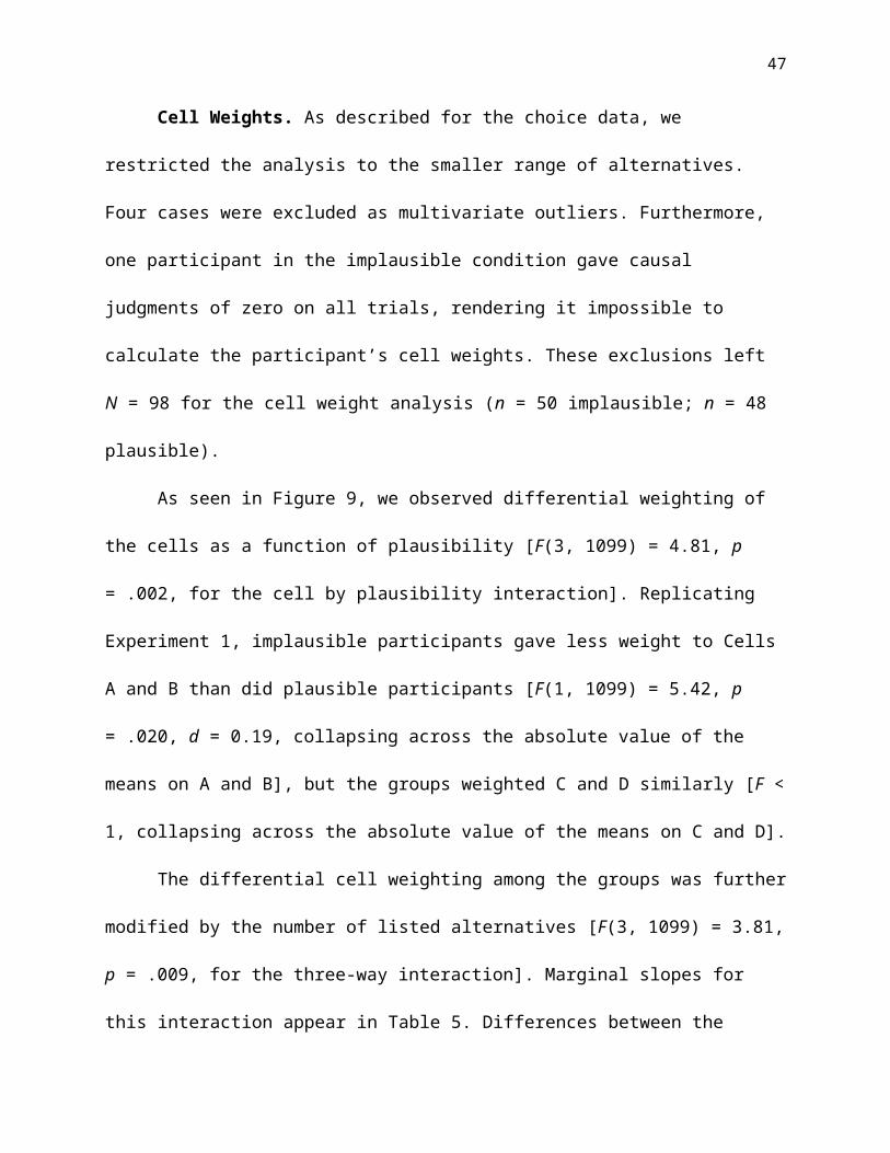
47

Table 1. Summary of the candidate causes used for the plausible and implausible

conditions for each of the four outcomes.

Condition Outcome

Skin Rash Car Accidents Plant Growth Stress

Plausible Hiking in

woods

Severed brake

lines

Adding fertilizer Having lots of

deadlines

Implausible Studying

vocabulary

Having leather

seats

Being in a blue

pot

Eating lots of

fruits & veggies

Note. Skin rash and car accident outcomes appeared in Experiments 1 and 3. All four

outcomes appeared in Experiments 2 and 4.

48

Table 2. Cell frequencies and objective contingencies for each of the trials in

Experiment 1.

Cell A Cell B Cell C Cell D phi

1 2 4 8 0.000

4 1 8 2 0.000

8 2 4 1 0.000

4 8 1 2 0.000

2 1 8 4 0.000

2 8 1 4 0.000

8 4 2 1 0.000

1 4 2 8 0.000

3 7 1 4 0.107

8 1 4 2 0.272

2 4 1 8 0.272

2 7 0 6 0.320

2 0 7 6 0.320

5 0 7 3 0.354

8 2 1 4 0.577

4 1 2 8 0.577

49

Table 3. Cell frequencies and objective contingencies for each of the trials in

Experiment 2.

A B C D phi

2 5 2 1 -0.356

1 2 5 2 -0.356

2 2 5 1 -0.356

2 5 1 2 -0.048

1 2 2 5 0.048

5 2 1 2 0.356

5 1 2 2 0.356

2 1 2 5 0.356

1 2 20 15 -0.238

15 20 2 1 -0.238

20 15 1 2 0.238

2 1 15 20 0.238

1 15 20 2 -0.847

2 20 15 1 -0.847

15 1 2 20 0.847

20 2 1 15 0.847

50

Table 4. Marginal slopes for predicting cell weights from number of alternatives listed in

Experiment 2.

Cell b β p

A 0.0040 0.06 .566

B -0.0122* -0.25* .032

C -0.0121~ -0.21~ .061

D 0.0045 0.09 .421

Note: SE on b was 0.01. p indicates test of slope against zero. * denotes significantly

from zero at p < .05; ~ at p < .10. Recall that cells B and C are normatively negatively

weighted. Thus, negative slopes on these cells indicate an increasing cell-weight as the

number of alternatives increases.

51

Table 5. Marginal slopes for predicting cell weight from number of listed alternatives as

a function of cell and plausibility of the causal mechanism in Experiment 4.

Implausible Causal

Mechanism

Plausible Causal

Mechanism

Simple Effects:

Implausible Vs.

Plausible

Cell b β b β

A 0.082* 0.23* -0.042 -0.12 p = .010

B -0.069* -0.20* -0.004 -0.01 p = .178

C -0.031 -0.09 0.041 0.16 p = .112

D 0.028 0.09 0.023 0.06 p = .898

Note: SE on b was 0.04. * denotes significantly from zero at p < .05. Recall that cells B

and C are normatively negatively weighted. Thus, negative slopes on these cells

indicate an increasing cell-weight as the number of alternatives increases.

52

Figure Captions

Figure 1. 2 x 2 Contingency Table with cell labels representing the number of times the

cause and the outcome were jointly present (Cell A), jointly absent (Cell D), or occurred

alone (Cells B and C, respectively).

Figure 2. Absolute value of cell weights based on posterior causal power resulting from

a weighted average of (A) causal power (Cheng, 1997) or (B) causal support (Griffiths &

Tenenbaum, 2005) and priors on the relation between the cause and outcome with

moderately common causes and outcomes [p(C) = p(E) = .50]. A prior of .9 indicated

high plausibility, .5 moderate plausibility, and .1 low plausibility.

Figure 3. Absolute value of the mean cell weights of Experiment 1. Error bars are ±1

SE.

Figure 4. Absolute value of mean cell weights in Experiment 2. Error bars are ±1 SE.

Figure 5. Scatterplot with regression slopes for predicting Cell B and C weights from the

number of alternatives listed in Experiment 2 (averaged over outcome and plausibility).

Note that because Cells B and C are normatively negatively weighted, increasing

negative values indicates an increase in the cell weight.

Figure 6. (A) Choice and (B) feedback screens in Experiment 3.

Figure 7. Scatterplot with regression slopes for predicting proportion of cause present

choices from the number of causes listed (averaged over outcome) for the (a)

implausible and (b) plausible conditions of Experiment 3.

Figure 8. Choice screen in Experiment 4.

Figure 9. Absolute value of mean cell weights of Experiment 4. Error bars are ±1 SE.

53

Figure 10. Regression slopes for predicting the mean cell weight of implausible

participants for Cells A and B in Experiment 4. Note, increasing negative values on Cell

B indicate an increase in weight on that cell.

54

Figure 1. 2 x 2 Contingency Table with cell labels representing the number of times the

cause and the outcome were jointly present (Cell A), jointly absent (Cell D), or occurred

alone (Cells B and C, respectively).

55

Figure 2.

A B

56

Figure 3.

57

Figure 4.

58

Figure 5.

-1

-.5

0

.5

1

Cell Weight

0 5 10 15 0 5 10 15

A Cell B B Cell C

Mean Number of Alternatives Listed

59

Figure 6.

A B

Mean Proportion of Cause Present Choices

60

Figure 7.

.2

.4

.6

.8

0 5 10 15

Mean Number of Listed Alternatives

0 5 10 15

A Implausible B Plausible

61

Figure 8

62

Figure 9.

63

Figure 10.

0

-1

1

Mean Cell Weight

0 5 10 15 0 5 10 15

A Implausible Cell A B Implausible Cell B

Mean Number of Listed Alternatives

64

Appendix A

Modeling Method and Results

Three models enhanced to represent plausible versus implausible causal

mechanisms are presented: power-PC (Cheng, 1997), causal support (Griffiths &

Tenenbaum, 2005), and sparse and strong (SS) priors (Lu et al., 2008). Each model’s

predictions were assessed by computing its measure of causal strength for 1000

randomly generated 2 x 2 contingency tables and then regressing that measure on the

tables’ cell frequencies. For each contingency table, the sample size N was first drawn

from a uniform distribution bounded by [100, 200]. Two draws of size N from a binomial

distribution with parameter p, representing the presence/absence of the cause and

effect, respectively, were then crossed to form a contingency table. A table yielding a

cause/effect correlation 0 was discarded and this process repeated until 1000 tables

were accumulated. Simulation results are reported for values of p = .1, .5, and .9,

corresponding to cases in which the cause and effect are both rare, occur with

probability ≈.5, or are both common.

Power-PC With Priors

The plausibility of the causal mechanism was rendered as a prior distribution

over causal power. Because power is a probability in the range [0-1], the prior was

represented as a beta distribution. The shape of a beta distribution is controlled by two

parameters, α and β, constrained to be positive real numbers. The mean of the prior

distribution, Beta (αprior, βprior), is αprior /(αprior + βprior), was set to either .1 (a prior belief that

causal power is low, corresponding to a causal mechanism of low plausibility), .5

65

(moderate plausibility), or .9 (high plausibility); the prior confidence in that estimate (i.e.,

how peaked the distribution is), represented by αprior + βprior, was held constant at 100.

(100 can be interpreted as the number of “prior observations.”) For each of the 1000

samples, the empirical causal power was calculated in the usual way:

pi=∆P i /(1−P(e∨ i)) where ∆ Pi=P (e∨i)−P(e∨ i) (Cheng, 1997). The parameters of a

beta distribution that characterizes the information about causal power inherent in the

sample were then derived: αempirical = piN and βempirical = (1 – pi)N, where N is the size of the

sample. The posterior distribution is given by Beta (αprior + αempirical, βprior + βempirical); the

posterior estimate of causal power was defined as the mean of the posterior. The

results of predicting the posterior causal power of the 1000 samples from the four cell

frequencies are shown in Figures 2 and A1B for the case in which the cause and effect

are both moderately common, that is p(C) p(E) .5.

As mentioned two additional runs of our simulation were conducted where C and

E were both rare (p = .1) or both common (.9). Although the weights of the cells relative

to each other changed (Cell A was most important when C and E were rare, Cell D was

most important when they were common), the effect of the prior was the same as in

Figure 2: As prior causal strength increased, Cells A and D decreased in importance

and B and C increased (compare Figure A1A – A1C).

Causal Support

Griffiths and Tenenbaum (2005) assume that causal judgments reflect learners’

beliefs in the (log of the) relative probability of two hypotheses, namely, that there is a

causal relationship between the two variables (“Graph 1”) and that there isn’t (“Graph

0”). This measure, causal support, is defined as,

66

support=log p (Graph1∨D)p (Graph0∨D)

=log p(D∨Graph1)p(D∨Graph0)

+ log p(Graph 1)p(Graph 0)

(1)

where D is the observed data. When the prior probabilities of the two hypotheses are

equal, Eq. 1 becomes,

support=log p (D∨Graph 1)p (D∨Graph 0)

(2)

where

p(D∨Graph1)=∫0

1

∫0

1

p(D∨w0 ,w1 ,Graph1) p(w0 ,w1∨Graph 1)d w0d w1

(3)

p(D∨Graph0)=∫0

1

p(D∨w0 ,Graph 0) p(w0∨Graph 0)dw0

(4)

w1 and w0 represent the strength of the candidate and alternative cause, respectively.

Griffiths and Tenenbaum make no assumptions about the causal powers in either

graph. Rather, they evaluate Eq. 3 by uniformly sampling over all possible values of w1

and w0. (Eq. 4 has an analytic solution.)

We elaborate causal support in two ways to represent plausibility. First, rather

than assuming a uniform prior on the causal power between the cause and effect

variable in Graph 1 (i.e., on w1), we make the same assumptions as we did in the

previous section, namely that the w1 prior is represented as a beta distribution with a

mean of .1, .5, or .9 (the number of “prior observations,” αprior + βprior, was to set to 10).

That is, for Graph 1 the prior over parameters becomes

67

p(w0 ,w1∨Graph 1)=p (w0∨Graph1) p (w1∨Graph1)

(5)

where p(w0∨Graph 1) is uniformly distributed and p(w1∨Graph1) is beta distributed with

parameters αprior and βprior.

For each of the 1000 data samples, Eq. 3 was evaluated by uniformly sampling

w1 and w0 a million times. For each of those samples, the prior (Eq. 5) was multiplied by

the likelihood of the data (see Griffiths & Tenenbaum, Eq. 7), to compute the posterior.

The mean of the posterior distribution that resulted was taken as the value of

p(D∨Graph1) and causal support was then computed according to Eq. 2. The 1000

values of support computed in this manner were regressed on the cell frequencies.

The results of this simulation revealed a pattern of cell weights qualitatively

similar to the prediction of Fugelsang and Thompson (2003): with decreases in

plausibility there is a decrease in cell weights for all cells (see Figure 2 and Figure A1D

to A1F). Although the same pattern of results obtained when C and E were both rare

(.1) or both common (.9), we further observed that like causal power, cell D was most

heavily weighted when C and E were common.

The second elaboration involves changing the prior probabilities of Graph 1 and

Graph 0 in Eq. 1 rather than placing a prior on w1 in Graph 1. Note that this elaboration

is based on a different sense of plausibility, one in which an “implausible” causal

mechanism is not necessarily weak but rather unlikely to exist and a “plausible” one is

not necessarily strong but rather likely to exist. In fact, this elaboration predicts no effect

of changing the prior probabilities of Graph 1 and Graph 0 on cell weights. Why it does

so is transparent from Eq. 1. Because any change to Eq. 1’s second term merely adds a

68

constant to causal support, no change to the weights is observed when it is regressed

onto the cell frequencies.

Strong and Sparse Priors (SS)

Lu et al. (2008) assume that causal strength judgments are influenced by a

“sparse and strong” (SS) prior on causal power that reflects learners’ biases that causes

are both strong and few in number. Applied to standard causal learning situations such

as those studied here, this assumption entails a prior in which C is either a strong cause

of E (and alternatives causes of E are weak or nonexistent) or C is a weak or

nonexistent cause of E (which is thus explained by strong alternative causes instead).

Although Lu et al. emphasize learning situations in which prior knowledge is absent and

so these generic priors dominate, they allow for the potential influence of prior

knowledge via specific priors. We model plausibility in this framework in the same way

as for causal power, namely, with (specific) priors in the form of a beta distribution that

reflect the prior expectation that power is weak (.1), moderate (.5), or strong (.9). (αprior +

βprior was held constant at 10.) The generic and specific priors were multiplied yielding,

p(w0 ,w1∨Graph 1)∞ (e− γw0−γ (1−w1)+e−γ (1−w0)− γw1)dbeta (w1∨α prior+1 , βprior+1)

(6)

where w1 and w0 again represent the strength of the candidate and alternative cause,

respectively, and dbeta is the Beta density function. Following Lu et al., the γ parameter,

which controls the strength of the SS priors, was set to 5. For each of the 1000 data

samples, the above prior was uniformly sampled over w1 and w0 a million times; for each

of those the posterior was computed by multiplying it with the likelihood of the data. The

69

estimate of causal strength was taken to be the mean value of w1 in the resulting

posterior distribution.

Unlike causal power and causal support, this model predicted different effects of

plausibility depending on whether C and E were rare or common. For rare events

(Figure A1G), the effects of plausibility on Cells A and B look like those of causal power

(Figure A1A): decreases in plausibility are associated with an increase in Cell A weight

and decrease in Cell B weight. When the events are common (Figure A1I), plausibility

results in decreases in weighting on most cells (more like causal support).

70

Figure Caption

Figure A1. Cell weight predictions with high (prior = .9), medium (prior = .5), and low

(prior = .1) prior plausibility of the causal relations for causal power (graphs A through

C), causal support (graphs D through F) and strong and sparse power (graphs G

through I) for rare (p = .1), moderately common (p = .5), and highly common (p = .9)

events.

71

Rarity Causal Power Causal Support Strong & SparseA D G

p = .10

B E H

p = .50

C F I

p = .90

72

Appendix B

Residual Covariance Structures and Random Effects Results

EXPERIMENT 1

Cell Weighting

Covariance Structure. Preliminary likelihood ratio tests suggested the need for

modeling different variances for the plausible and implausible conditions [ (1) =

17.40, p < .001, compared to homogeneous variance and covariance]. Variance for the

implausible and plausible groups was 0.082 and 0.122, respectively.

ICC and Random Effects. The intraclass correlation coefficient (ICC) was 0.00,

indicating little within-participant correlation among the cell weights. As to be expected

given the ICC of 0, variance attributable to the random effects of participant was =

0.00, SE = 0.002.

EXPERIMENT 2

Number of Causes Listed

Covariance Structure. The covariance structure with homogeneous variances

and zero covariance best fit the data (all ps > .81 relative to more complex structures).

ICC and Random Effects. The ICC was .46, indicating a moderate within-

participant correlation in the number of causes listed. The model yielded significant

effects of participants' random intercepts, = 5.57, SE = 0.91, Z =6.14, p < .001.

Cell Weighting

Covariance Structure. We modeled different variances for each of the four cells

in the residual covariance matrix [ (3) = 21.22, p < .001, compared to homogeneous

2

20

20

2

73

variance structure]. Variances for Cells A, B, C, and D were 0.159, 0.108, .140, and

0.105, respectively.

ICC and Random Effects. The ICC was 0.00 and variance attributable to the

random effects of participants was = 0.00, SE = 0.00.

EXPERIMENT 3

Number of Causes Listed

Covariance Structure. The likelihood ratio tests suggested the need for

modeling different variances for plausibility with covariances equal to zero [ (3) =

30.08, p < .001, compared to homogeneous variances]. Variances for the implausible

and plausible conditions were 4.50 and 1.62, respectively.

ICC and Random Effects. The ICC was .23, indicating a small to moderate

within-participant correlation in the number of causes listed. Consistent with the

moderate ICC, participants' random intercepts reached significance, = 4.61, SE =

0.99, Z = 4.64, p < .001.

Cause Present Choices

Covariance Structure. We modeled different variances for plausibility and

presentation order [ (3) = 25.17, p < .001, compared to homogeneous variance

structure]. Variance for the implausible, cause-present first condition was 0.009; for the

implausible, cause-present second it was 0.009; for the plausible, cause-present first it

was 0.005; and for the plausible, cause-present second it was 0.023.

20

2

20

2

74

ICC and Random Effects. The ICC was .26, indicating a small to moderate

within-participant correlation. The random effect of participants’ intercepts reached

significance, = 0.0024, SE = 0.0011, z = 2.71, p = .030.

EXPERIMENT 4

Number of Causes Listed

Covariance Structure. We modeled different variances for each outcome with

covariances equal to zero [ (3) = 49.37, p < .001, compared to homogeneous

variance structure]. Variances for the skin rash, car accidents, plant growth, and stress

outcomes were 1.99, 5.32, 1.14, and 6.51, respectively.

ICC and Random Effects. The ICC was .48, indicating a moderate within-

participant correlation. Consistent with the moderate ICC, participants random

intercepts reached significance, = 3.89, SE = 0.64, Z = 6.06, p < .001.

Cause Present Choices

Covariance Structure. We modeled different variances for plausibility and

option order [ (3) = 8.69, p = .034, compared to homogeneous variance structure].

Variance for the implausible, cause-present left condition was 0.011; for the implausible,

cause-present right it was 0.011; for the plausible, cause-present left it was 0.007; and

for the plausible, cause-present right it was 0.015.

ICC and Random Effects. The ICC was .34, indicating a small to moderate

within-participant correlation. The random effect of participants’ intercepts reached

significance, = 0.005, SE = 0.001, z = 4.36, p < .001.

20

2

20

2

20

75

Cell Weighting

Covariance Structure. We modeled different variances for outcome [2 (2) =

18.62, p < .001, compared to homogeneous variance structure]. Variance for skin

rashes was 0.762; for accidents it was 1.196; for plant growth it was 0.970 and for

stress it was 1.144.

ICC and Random Effects. The ICC was .00, indicating no within-participant

correlation. Accordingly, the random effect of participants’ intercepts did not reach

significance, 20 = 0.000, SE = 0.000, z = 0.22, p > .05.

76

Appendix C

Cell Weight Results for Cambridge Participants in Experiment 1

Among the 48 Cambridge participants (n = 24 each in the plausible and

implausible conditions), none were identified as outliers. As can be seen in Figure C1,

there was a tendency for implausible participants to place less weight on Cells A and B,

and more weight on Cells C and D, relative to plausible participants [F(3, 314) = 4.42, p

= .005, for the plausibility by cell interaction]. However, the difference between the

groups only reached significance for Cells A and D [p = .046, d = 0.50 for Cell A; p

= .729, d = 0.05 for Cell B; p = .236, d = 0.26 for Cell C; and p = .005, d = 0.74 for Cell

D]. This pattern of results is qualitatively different than that observed among the US

implausible participants, who when compared to the plausible group, weighted Cells A

and B less, but Cells C and D about the same. The results of the UK sample are more

commensurate with the positive test prediction introduced here. While these results

suggest potential cultural differences either in the cell weighting or in the interpretation

of the causal cover stories, it was beyond the scope of the current paper to further

investigate these.

77

Figure C1. Absolute value of the mean cell weights for the UK participants in

Experiment 1.

78

Appendix D

Cover Story Piloting

We conducted a pilot study to identify additional outcomes to be used in cover

stories for Experiments 2 and 4. Seton Hall University students (n = 102; 70 female)

received course credit for completing the study. Participants tested in the laboratory in

groups of up to four, completing the study using Survey Monkey. They were asked to

list as many possible causes as they could think of for these randomly-ordered

outcomes: (1) car accident; (2) skin rash; (3) plant growth; (4) colon cancer; (5)

chemical reaction; (6) stress; (7) fatigue; and (8) losing one’s job. Each outcome was

presented one at a time. Participants listed all the causes they could think for each by

typing their responses in the response box and then hit “submit” to continue to the next

outcome. The outcomes were selected based on conversations with our respective

research teams and solicitations on social networking sites. We hoped to identify a set

of outcomes that would vary in the number of causes they would elicit. Table D1 depicts

the number of causes participants listed for each outcome. Repeated-measures

ANOVA indicated a significant effect of outcome type, F(7,707) = 63.88, p < .001.

Results of Tukey’s HSD post-hoc are indicated with superscripts in Table D1.

Table D1. Number of causes listed in the pilot study as a function of outcome.

Outcome M SD

Stressa 7.07 3.70

Car Accidenta 7.01 4.06

Lose One's Jobb 5.76 3.08

Fatigueb,c 5.09 3.82

Plant Growingc,d 4.33 1.98

79

Skin Rashd 4.04 2.04

Colon Cancere 2.56 1.57

Chemical Reactione 2.30 1.62

Note: Superscripts indicate outcomes not significantly different via Tukey’s HSD.