ATS 515 – Advanced Topics in GIS

Student Instruction, 28 February 2012

Identifying landslide triggers and estimating inundation zones in the Monte Sano Nature Preserve

Overall Goals

Pinpoint locations most prone to slope failure in the Monte Sano Nature Preserve (Land Trust) Delineate rock fall inundation hazard zones from those areas

Specific Objectives

Perform basic surface and hydrology analyses of high resolution digital terrain model (DTM), including: Fill, Flow Direction, Flow Accumulation, Stream Link, Slope and Hillshade, among other complementary tools

Predict the locations of unstable conditions as a function of slope and upslope contributing area (simplification of SHALSTAB – shallow slope stability model – criterion).

From these locations, simulate rock avalanches to estimate inundation hazard areas using the LAHARZ software in Arc Workstation.

(time permitting) Visualize results in ArcScene.

Concepts

The term “mass movement” encapsulates pretty much any large volume of material that moves downslope under the force of gravity (Abbott 2012)

Significant landslide hazards exist in the southeastern US, particularly in areas with steep slopes along the weathering Appalachian mountains. Within Madison County, Alabama, moderate to very high susceptibility has been identified across Monte Sano (Geological Survey of Alabama 2011).

LAHARZ was originally developed to estimate lahar inundation zones along volcanic flanks (Schilling 1998). It can also be used for debris flows and rock falls. These types of mass movement all have very rapid to extremely rapid rates of movement but have different water contents (Abbott 2012).

Slope stability models can be used to identify “triggers,” or specific points more prone to causing landslides. The main factors needed to define unstable conditions include sufficiently steep slope, availability of soil or other debris, and enough water to trigger and perpetuate a flow (Montgomery and Dietrich 1994; Deitrich et al 1998)

Inundation zones can be objectively delineated given a terrain model and initial volumes. Observation of lahars, debris flows and rock avalanches have yielded relationships between volume , planimetric inundation area and cross-sectional inundation area (Iverson et al 1998)

Exercise

Part I: Identify landslide trigger cells

1. Open a new empty ArcMap project, and add the layer called ms_fill. a. What is the projection? ________________________________b. What is the horizontal resolution (include units)? _________________________c. What is the area in each cell? _______________________

2. Make a hillshade of the DEM. Name it ms_fillsh. Be sure to save this and all other outputs in the same directory as ms_fill!

3. Calculate flow direction to determine the direction from each cell to its steepest downslope neighbor (i.e., which direction the majority of water would flow across the surface). Find the tool in Spatial Analyst Tools / Hydrology / Flow Direction. Make sure to use your filled DEM as your input surface raster. Name the output flow direction raster: ms_dir:

4. Observe the output. How many values are there? _____________If your flow direction does not look like the layer below, make sure you started with the filled DEM.

5. Run flow accumulation to calculate the how many upstream cells flow into each cell. Select ms_dir as the flow direction raster, name the output ms_flac, keep the input weight raster blank, and change the output data type to Integer:

6. Change the symbology of the resulting flow accumulation layer (using Histogram Equalize stretch), drag the hillshade layer on top and change its transparency to 60%.

7. Zoom to the area shown above, and “identify” or query the values of ms_flac. These values correspond to the number of upstream cells that flow into the cell you are querying. We will use these channels to determine starting points for small landslides or rock avalanches that could turn into larger debris flows.

8. Now we will separate the cells that represent streams/small rivulets from those that do not. Open the Con tool in Spatial Analyst Tools / Conditional / Con, select ms_flac as the input conditional raster, Expression: value > 2000; Input true: 1; Input false: 0; Output raster ms_str:

9. Your result should show a grid with two values: 0 and 1. Cells with a value of 1 represent streams and small rivulets. The value 2000 was chosen based on the resolution of the DEM and the density of streams/rivulets we wanted to see. For other cases, you’ll need to play with this value to find the right threshold.

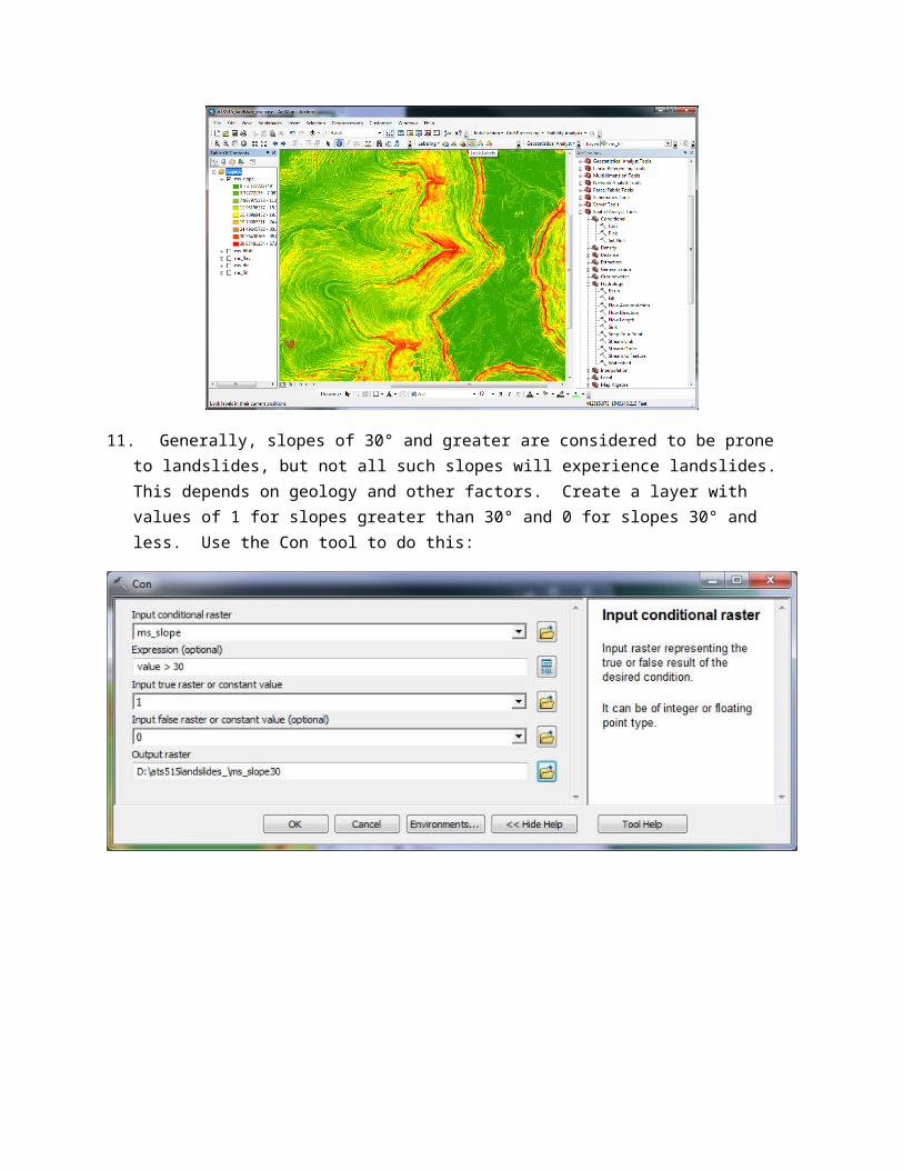
10. Next, we will analyze the slope for steepness. Calculate slope in degrees, naming the output ms_slope. Explore the values of these slopes.

11. Generally, slopes of 30° and greater are considered to be prone to landslides, but not all such slopes will experience landslides. This depends on geology and other factors. Create a layer with values of 1 for slopes greater than 30° and 0 for slopes 30° and less. Use the Con tool to do this:

12. Beyond identifying cells with slopes > 30°, we can also locate blocks of continuously steep slopes. This is important because short, steep slopes may cause small slumps that do not result in large landslides, while larger areas of steep slopes may lead to larger landslides that bulk up and travel much further with greater volumes. Using neighborhood functions, we will identify cells whose neighbors in a 10x10 radius are also steep. We will not limit this to all of the neighboring cells but instead 95% of those cells. Open the Focal Statistics Tool under Spatial Analyst Tools / Neighborhood to calculate the SUM of the values within a 10x10 neighborhood of each input cell. Fill in the fields accordingly, and name the output area10x10:

13. Open the Con tool to separate the cells with values > 95 from the rest. Name the output area095:

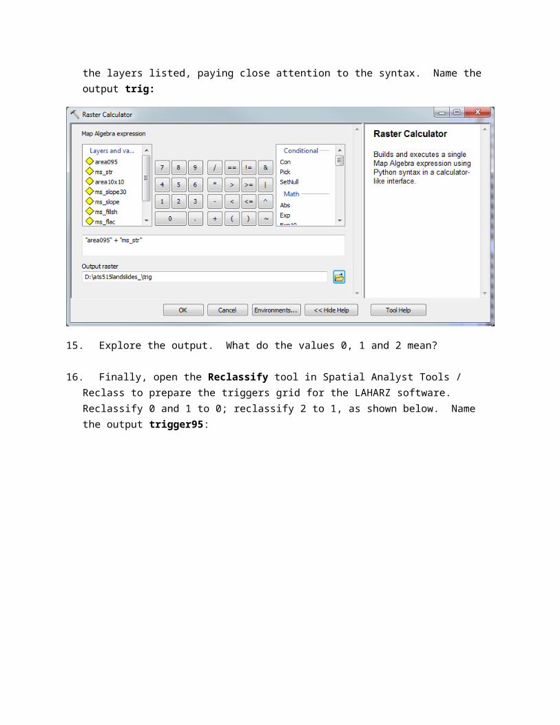
14. This results in all steep-sloped cells that are also surrounded by steep slopes. The final step to identify our landslide triggers is to select these steep-slope cells that intersect the streams or rivulets we created earlier. To do this, we can “add” the two layers area095 and ms_str together using Raster Calculator located in Spatial Analyst Tools / Map Algebra. Enter the expression using the layers listed, paying close attention to the syntax. Name the output trig:

15. Explore the output. What do the values 0, 1 and 2 mean?

16. Finally, open the Reclassify tool in Spatial Analyst Tools / Reclass to prepare the triggers grid for the LAHARZ software. Reclassify 0 and 1 to 0; reclassify 2 to 1, as shown below. Name the output trigger95:

This should result in a layer with only two values (0 and 1), where the very few cells with a value of 1 meet all of our requirements for landslide triggers. We will now continue to delineate potential inundation hazard zones from these points. Save and minimize your ArcMap window.

Part II: Estimate potential landslide inundation hazard zones

1. From the start menu, navigate to ArcInfo

Workstation and open Arc.

2. We now need to specify the working directories. From the Arc prompt, type the following:

&amlpath _______ from windows explorer, click and drag the aml_laharz_2.7 folder to bring in the complete location.

&menupath _______ same as above

w ____________ click and drag the directory with all of your spatial analysis grids you just prepared.

Example:

3. Run LAHARZ by typing: &r laharz

4. Click “Create Inundation Area”

5. Click “Rock Avalanche” and “Continue”

6. Enter msrock for the area name prefix. Type in four volumes: 1000, 3000, 10000 and 30000. Be sure to hit <Enter> after typing each volume. Click “Continue.”

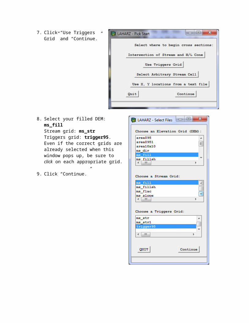
7. Click “Use Triggers Grid” and “Continue.”

8. Select your filled DEM: ms_fill Stream grid: ms_strTriggers grid: trigger95.Even if the correct grids are already selected when this window pops up, be sure to click on each appropriate grid.

9. Click “Continue.”

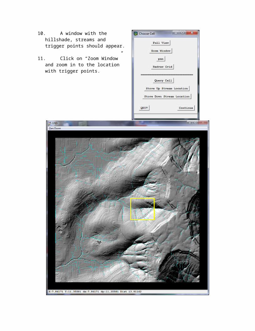
10. A window with the hillshade, streams and trigger points should appear.

11. Click on “Zoom Window” and zoom in to the location with trigger points.

12. Click on “Query Cell,” then click on one of the pink trigger cells. Check to see that the Arc window says “VALID CELL VALUE.” If it says “INVALID CELL VALUE,” click on the “Query Cell” button and try again.

13. Once you have selected a valid cell, click the “Store Up Stream Location button.”

14. Click “Full View” to return to the full extent.

15. Click “Zoom Window” and zoom to the end of a stream at the bottom half of the left edge of the grid.

16. Click on “Query Cell,” and click one of the blue cells in the stream at the left edge of the grid.

17. If the Arc window says “VALID CELL,” click the “Store Down Stream Location.” If not, try again.

18. Click “Continue” to begin calculating inundation areas. This may take a few minutes. For larger volumes and higher resolution DEMs, this could take hours.

19. When the creation of inundation zones is complete, click on the “Quit” button. Then in the Arc: prompt type “quit” and hit <Enter>.

20. Open the results in ArcMap and apply appropriate symbology. Here are results for a few different runs with hiking trails for reference.

It may be more informative to show these results from a different perspective, such as in ArcScene or Google Earth.

Consider:

1. What were our inputs for the trigger and inundation hazard zones?

2. What are the assumptions in the models we used?

3. What are the uncertainties, and how do we deal with these?

4. How can we improve these models?

Note: Part I could have also been completed in a few minutes using the following 10 Arc Workstation commands in the grid module:

Arc: gridGrid: ms_dir = flowdirection(ms_fill) Grid: ms_flac = flowaccumulation(ms_dir) Grid: ms_slope = slope(ms_fill) Grid: ms_slope30 = con(ms_slope > 30, 1, 0) Grid: area10x10 = focalsum(ms_slope30, rectangle, 10, 10) Grid: area095 = con(area10x10 > 95, 1, 0) Grid: ms_str = con(ms_flac > 2000, 1, 0) Grid: trigger95 = con(ms_str == 0, 0, con(area095 == 1, 1)) Grid: quit

Acknowledgements

This exercise was modified and reformatted from a LAHARZ tutorial written for Mt. Hood, provided by Julia Griswold, Steve Schilling and Jon Major of the USGS. My participation in the LAHARZ workshop in El Salvador in January of 2012 was funded by USAID/NASA through the SERVIR program and offered me the opportunity to learn about the software directly from the people who created it.

Digital elevation model data for Monte Sano was provided by the City of Huntsville GIS Department through Robert Griffin.

References

Abbott, P.L., 2011. Natural Disasters. 8th Ed. McGraw-Hill. 512 pp.

Dietrich, W.E., Real de Asua, R., Coyle, J., Orr, B. and M. Trso, 1998 “A validation study of the shallow slope stability model, SHALSTAB, in forested lands of Northern California.” UC Berkeley, 59 pp.

Geological Survey of Alabama, 2011. Susceptibility to Landslides in Alabama. Poster by Ebersole, S.M., Driskell, S., and A.M. Tavis.

Griswold, J.P., and R.M. Iverson, 2007. “Mobility Statistics and Automated Hazard Mapping for Debris Flows and Rock Avalanches.” USGS Scientific Investigations Report 2007-5276.

Iverson, R.M., Schilling, S.P., and J.W. Vallance, 1998. “Objective delineation of lahar-inundation hazard zones.” Geological Society of America Bulletin 110: 972-984.

Montgomery, D.R., and W.E. Dietrich, 1994. “A physically-based model for topographic control on shallow landsliding.” Water Resources Research 30: 1153-1171.

Schilling, S.P., 1998. “LAHARZ: GIS programs for automated mapping of lahar-inundation hazard zones.” USGS Open-File Report 98-638.