Embed Size (px)
Citation preview

Sociology 7704: Regression Models for Categorical DataInstructor: Natasha Sarkisian
OLS Regression Assumptions
A1. All independent variables are quantitative or dichotomous, and the dependent variable is quantitative, continuous, and unbounded. All variables are measured without error.A2. All independent variables have some variation in value (non-zero variance).A3. There is no exact linear relationship between two or more independent variables (no perfect multicollinearity).A4. At each set of values of the independent variables, the mean of the error term is zero.A5. Each independent variable is uncorrelated with the error term.A6. At each set of values of the independent variables, the variance of the error term is the same (homoscedasticity). A7. For any two observations, their error terms are not correlated (lack of autocorrelation). A8. At each set of values of the independent variables, error term is normally distributed. A9. The change in the expected value of the dependent variable associated with a unit increase in an independent variable is the same regardless of the specific values of other independent variables (additivity assumption).A10. The change in the expected value of the dependent variable associated with a unit increase in an independent variable is the same regardless of the specific values of this independent variable (linearity assumption).
A1-A7: Gauss-Markov assumptions: If these assumptions hold, the resulting regression estimates are BLUE (Best Linear Unbiased Estimates).
Unbiased: if we were to calculate that estimate over many samples, the mean of these estimates would be equal to the mean of the population (i.e., on average we are on target).
Best (also known as efficient): the standard deviation of the estimate is the smallest possible (i.e., not only are we on target on average, but we don’t deviate too far from it).
If A8-A10 also hold, the results can be used appropriately for statistical inference (i.e., significance tests, confidence intervals).
OLS Regression diagnostics and remedies
1. Multivariate NormalityOLS is not very sensitive to non-normally distributed errors but the efficiency of estimators decreases as the distribution substantially deviates from normal (especially if there are heavy tails). Further, heavily skewed distributions are problematic as they question the validity of the mean as a measure for central tendency and OLS relies on means. Therefore, we usually test for nonnormality of residuals’ distribution and if it's found, attempt to use transformations to remedy the problem.
To test normality of error terms distribution, first, we generate a variable containing residuals:. reg agekdbrn educ born sex mapres80 age
1
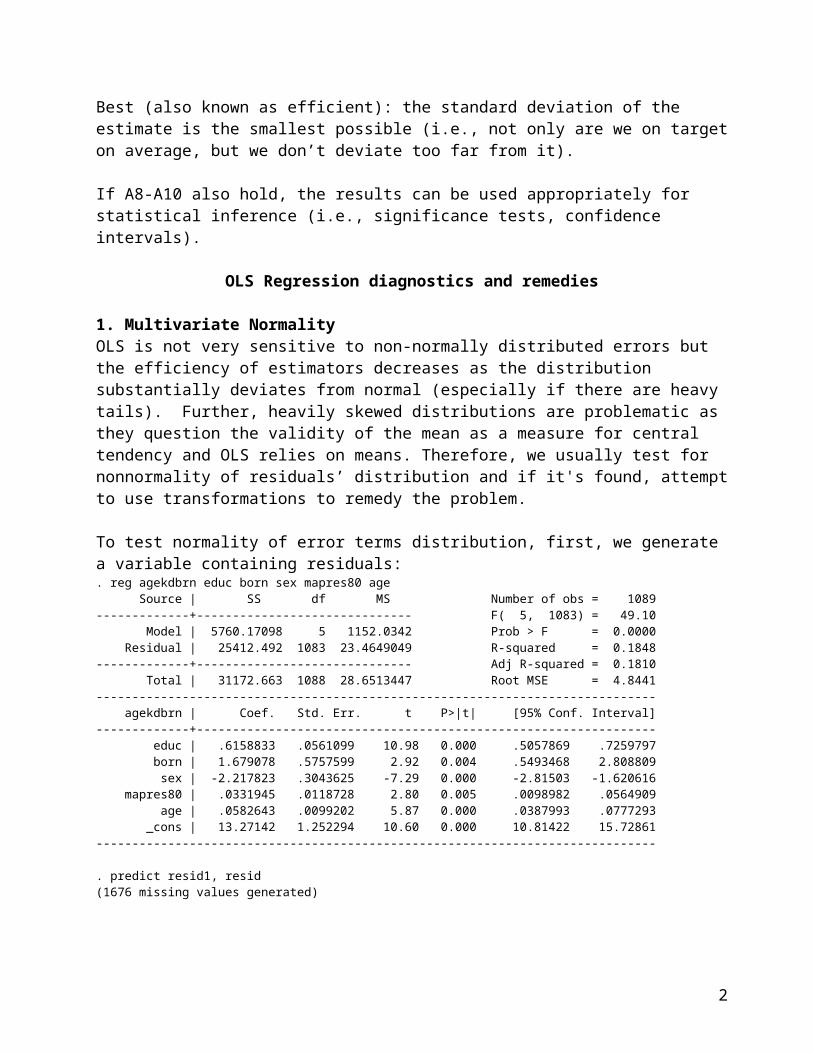
Source | SS df MS Number of obs = 1089-------------+------------------------------ F( 5, 1083) = 49.10 Model | 5760.17098 5 1152.0342 Prob > F = 0.0000 Residual | 25412.492 1083 23.4649049 R-squared = 0.1848-------------+------------------------------ Adj R-squared = 0.1810 Total | 31172.663 1088 28.6513447 Root MSE = 4.8441------------------------------------------------------------------------------ agekdbrn | Coef. Std. Err. t P>|t| [95% Conf. Interval]-------------+---------------------------------------------------------------- educ | .6158833 .0561099 10.98 0.000 .5057869 .7259797 born | 1.679078 .5757599 2.92 0.004 .5493468 2.808809 sex | -2.217823 .3043625 -7.29 0.000 -2.81503 -1.620616 mapres80 | .0331945 .0118728 2.80 0.005 .0098982 .0564909 age | .0582643 .0099202 5.87 0.000 .0387993 .0777293 _cons | 13.27142 1.252294 10.60 0.000 10.81422 15.72861------------------------------------------------------------------------------
. predict resid1, resid(1676 missing values generated)
Next, we can use any of the tools we used above to evaluate the normality of distribution for this variable. For example, we can construct the qnorm plot:. qnorm resid1
-20
-10
010
20R
esid
uals
-20 -10 0 10 20Inverse Normal
In this case, residuals deviate from normal quite substantially. We could check whether transforming the dependent variable using the transformation we identified above would help us:. quietly reg agekdbrnrr educ born sex mapres80 age. predict resid2, resid(1676 missing values generated). qnorm resid2
-.05
0.0
5.1
Res
idua
ls
-.05 0 .05Inverse Normal
2
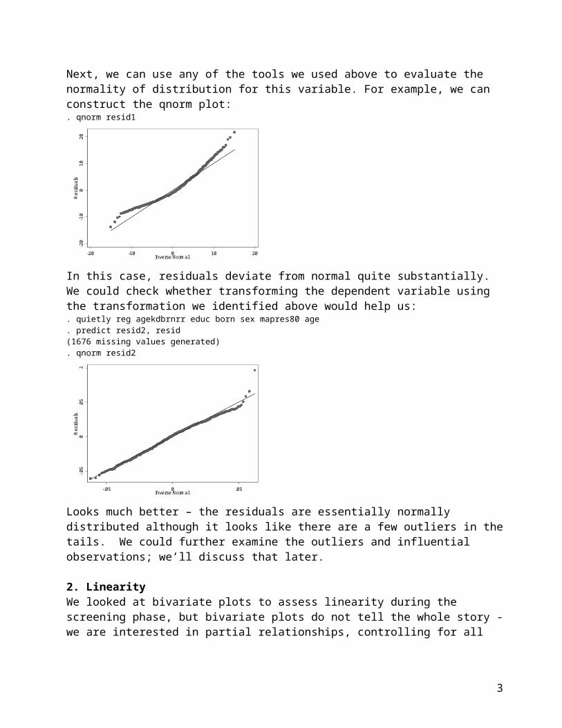
Looks much better – the residuals are essentially normally distributed although it looks like there are a few outliers in the tails. We could further examine the outliers and influential observations; we’ll discuss that later.
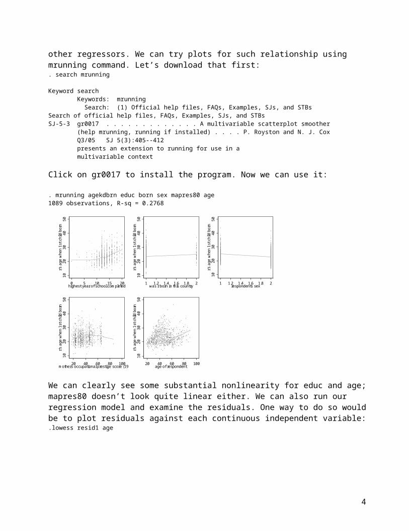
2. LinearityWe looked at bivariate plots to assess linearity during the screening phase, but bivariate plots do not tell the whole story - we are interested in partial relationships, controlling for all other regressors. We can try plots for such relationship using mrunning command. Let’s download that first:. search mrunning
Keyword search Keywords: mrunning Search: (1) Official help files, FAQs, Examples, SJs, and STBsSearch of official help files, FAQs, Examples, SJs, and STBsSJ-5-3 gr0017 . . . . . . . . . . . . . A multivariable scatterplot smoother (help mrunning, running if installed) . . . . P. Royston and N. J. Cox Q3/05 SJ 5(3):405--412 presents an extension to running for use in a multivariable context
Click on gr0017 to install the program. Now we can use it:
. mrunning agekdbrn educ born sex mapres80 age1089 observations, R-sq = 0.2768
1020
3040
50r's
age
whe
n 1s
t chi
ld b
orn
0 5 10 15 20highest year of school completed
1020
3040
50r's
age
whe
n 1s
t chi
ld b
orn
1 1.2 1.4 1.6 1.8 2was r born in this country
1020
3040
50r's
age
whe
n 1s
t chi
ld b
orn
1 1.2 1.4 1.6 1.8 2respondents sex
1020
3040
50r's
age
whe
n 1s
t chi
ld b
orn
20 40 60 80 100mothers occupational prestige score (1980)
1020
3040
50r's
age
whe
n 1s
t chi
ld b
orn
20 40 60 80 100age of respondent
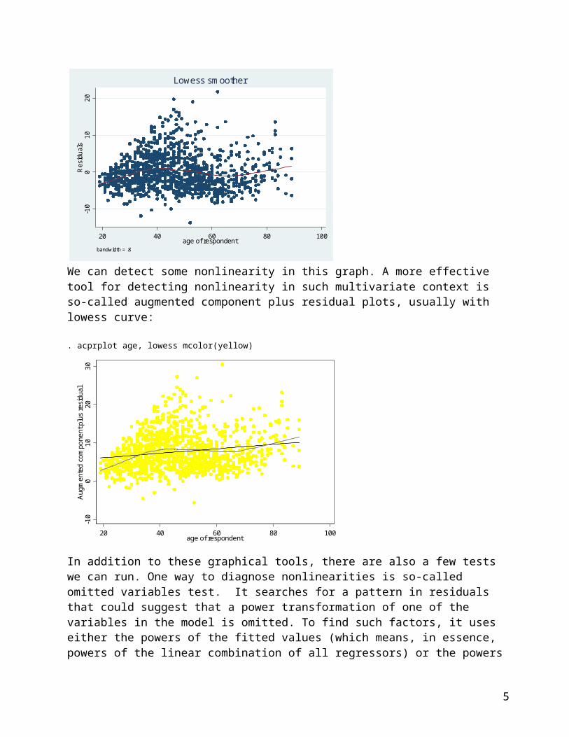
We can clearly see some substantial nonlinearity for educ and age; mapres80 doesn’t look quite linear either. We can also run our regression model and examine the residuals. One way to do so would be to plot residuals against each continuous independent variable:.lowess resid1 age
3
-10
010
20R
esid
uals
20 40 60 80 100age of respondent
bandwidth = .8
Lowess smoother
We can detect some nonlinearity in this graph. A more effective tool for detecting nonlinearity in such multivariate context is so-called augmented component plus residual plots, usually with lowess curve:
. acprplot age, lowess mcolor(yellow)
-10
010
2030
Aug
men
ted
com
pone
nt p
lus
resi
dual
20 40 60 80 100age of respondent
In addition to these graphical tools, there are also a few tests we can run. One way to diagnose nonlinearities is so-called omitted variables test. It searches for a pattern in residuals that could suggest that a power transformation of one of the variables in the model is omitted. To find such factors, it uses either the powers of the fitted values (which means, in essence, powers of the linear combination of all regressors) or the powers of individual regressors in predicting Y. If it finds a significant relationship, this suggests that we probably overlooked some nonlinear relationship.
. ovtestRamsey RESET test using powers of the fitted values of agekdbrn Ho: model has no omitted variables F(3, 1080) = 2.74 Prob > F = 0.0423
4
. ovtest, rhs(note: born dropped due to collinearity)(note: sex dropped due to collinearity)(note: born^3 dropped due to collinearity)(note: born^4 dropped due to collinearity)(note: sex^3 dropped due to collinearity)(note: sex^4 dropped due to collinearity)
Ramsey RESET test using powers of the independent variables Ho: model has no omitted variables F(11, 1074) = 14.84 Prob > F = 0.0000
Looks like we might be missing some nonlinear relationships. We will, however, also explicitly check for linearity for each independent variable. We can do so using Box-Tidwell test. First, we need to download it:
. net search boxtid(contacting http://www.stata.com)
3 packages found (Stata Journal and STB listed first)-----------------------------------------------------
sg112_1 from http://www.stata.com/stb/stb50 STB-50 sg112_1. Nonlin. reg. models with power or exp. func. of covar. / STB insert by / Patrick Royston, Imperial College School of Medicine, UK; / Gareth Ambler, Imperial College School of Medicine, UK. / Support: [email protected] and [email protected] / After installation, see
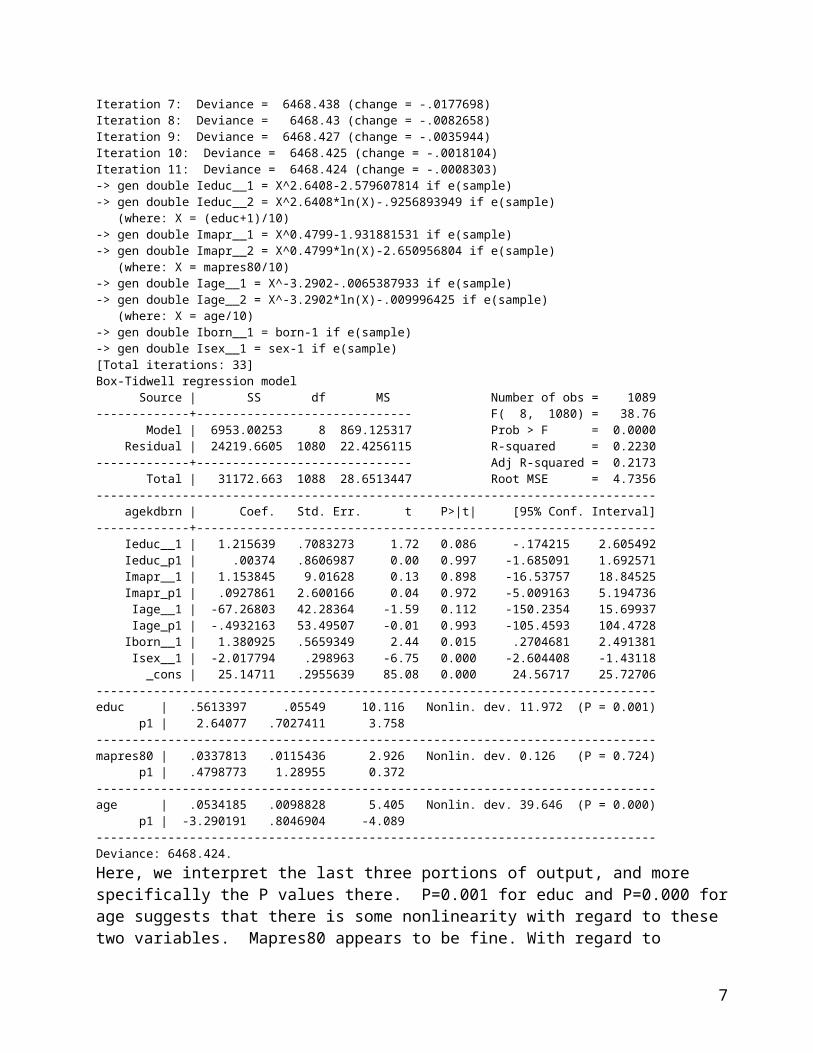
We select this first one, sg112_1, and install it. Now use it: . boxtid reg agekdbrn educ born sex mapres80 ageIteration 0: Deviance = 6483.522Iteration 1: Deviance = 6470.107 (change = -13.41466)Iteration 2: Deviance = 6469.55 (change = -.5577601)Iteration 3: Deviance = 6468.783 (change = -.7663782)Iteration 4: Deviance = 6468.6 (change = -.1832873)Iteration 5: Deviance = 6468.496 (change = -.103788)Iteration 6: Deviance = 6468.456 (change = -.0399491)Iteration 7: Deviance = 6468.438 (change = -.0177698)Iteration 8: Deviance = 6468.43 (change = -.0082658)Iteration 9: Deviance = 6468.427 (change = -.0035944)Iteration 10: Deviance = 6468.425 (change = -.0018104)Iteration 11: Deviance = 6468.424 (change = -.0008303)-> gen double Ieduc__1 = X^2.6408-2.579607814 if e(sample) -> gen double Ieduc__2 = X^2.6408*ln(X)-.9256893949 if e(sample) (where: X = (educ+1)/10)-> gen double Imapr__1 = X^0.4799-1.931881531 if e(sample) -> gen double Imapr__2 = X^0.4799*ln(X)-2.650956804 if e(sample) (where: X = mapres80/10)-> gen double Iage__1 = X^-3.2902-.0065387933 if e(sample) -> gen double Iage__2 = X^-3.2902*ln(X)-.009996425 if e(sample) (where: X = age/10)-> gen double Iborn__1 = born-1 if e(sample) -> gen double Isex__1 = sex-1 if e(sample) [Total iterations: 33]Box-Tidwell regression model Source | SS df MS Number of obs = 1089-------------+------------------------------ F( 8, 1080) = 38.76 Model | 6953.00253 8 869.125317 Prob > F = 0.0000 Residual | 24219.6605 1080 22.4256115 R-squared = 0.2230
5
-------------+------------------------------ Adj R-squared = 0.2173 Total | 31172.663 1088 28.6513447 Root MSE = 4.7356------------------------------------------------------------------------------ agekdbrn | Coef. Std. Err. t P>|t| [95% Conf. Interval]-------------+---------------------------------------------------------------- Ieduc__1 | 1.215639 .7083273 1.72 0.086 -.174215 2.605492 Ieduc_p1 | .00374 .8606987 0.00 0.997 -1.685091 1.692571 Imapr__1 | 1.153845 9.01628 0.13 0.898 -16.53757 18.84525 Imapr_p1 | .0927861 2.600166 0.04 0.972 -5.009163 5.194736 Iage__1 | -67.26803 42.28364 -1.59 0.112 -150.2354 15.69937 Iage_p1 | -.4932163 53.49507 -0.01 0.993 -105.4593 104.4728 Iborn__1 | 1.380925 .5659349 2.44 0.015 .2704681 2.491381 Isex__1 | -2.017794 .298963 -6.75 0.000 -2.604408 -1.43118 _cons | 25.14711 .2955639 85.08 0.000 24.56717 25.72706------------------------------------------------------------------------------educ | .5613397 .05549 10.116 Nonlin. dev. 11.972 (P = 0.001) p1 | 2.64077 .7027411 3.758------------------------------------------------------------------------------mapres80 | .0337813 .0115436 2.926 Nonlin. dev. 0.126 (P = 0.724) p1 | .4798773 1.28955 0.372------------------------------------------------------------------------------age | .0534185 .0098828 5.405 Nonlin. dev. 39.646 (P = 0.000) p1 | -3.290191 .8046904 -4.089------------------------------------------------------------------------------Deviance: 6468.424.Here, we interpret the last three portions of output, and more specifically the P values there. P=0.001 for educ and P=0.000 for age suggests that there is some nonlinearity with regard to these two variables. Mapres80 appears to be fine. With regard to remedies, the process here is the same as we discussed earlier when talking about bivariate linearity. Once remedies are applied, it is a good idea to retest using these multivariate screening tools.
3. Outliers, Leverage Points, and Influential Observations
A single observation that is substantially different from other observations can make a large difference in the results of regression analysis. For this reason, unusual observations (or small groups of unusual observations) should be identified and examined. There are three ways that an observation can be unusual:
Outliers: In univariate context, people often refer to observations with extreme values (unusually high or low) as outliers. But in regression models, an outlier is an observation that has unusual value of the dependent variable given its values of the independent variables – that is, the relationship between the dependent variable and the independent ones is different for an outlier than for the other data points. Graphically, an outlier is far from the pattern defined by other data points. Typically, in a regression model, an outlier has a large residual.
Leverage points: An observation with an extreme value (either very high or very low) on a single predictor variable or on a combination of predictors is called a point with high leverage. Leverage is a measure of how far a value of an independent variable deviates from the mean of that variable. In the multivariate context, leverage is a measure of each observation’s distance from the multidimensional centroid in the space formed by all the predictors. These leverage points can have an effect on the estimates of regression coefficients.
6
Influential Observations: A combination of the previous two characteristics produces influential observations. An observation is considered influential if removing the observation substantially changes the estimates of coefficients. Observations that have just one of these two characteristics (either an outlier or a high leverage point but not both) do not tend to be influential.
Thus, we want to identify outliers and leverage points, and especially those observations that are both, to assess and possibly minimize their impact on our regression model. Furthermore, outliers, even when they are not influential in terms of coefficient estimates, can unduly inflate the error variance. Their presence may also signal that our model failed to capture some important factors (i.e., indicate potential model specification problem).
In the multivariate context, to identify outliers, we want to find observations with high residuals; and to identify observations with high leverage, we can use the so-called hat-values -- these measure each observation’s distance from the multidimensional centroid in the space formed by all the regressors. We can also use various influence statistics that help us identify influential observations by combining information on outlierness and leverage.
To obtain these various statistics in Stata, we use predict command. Here are some values we can obtain using predict, with the rule-of-thumb cutoff values for statistics used in outlier diagnostics:
Predict option Result Cutoff value (n=sample size, k=parameters)
xb xb, fitted values (linear prediction); the default
stdp standard error of linear predictionresiduals residualsstdr standard error of the residualrstandard standardized residuals (residuals divided by
standard error)rstudent studentized (jackknifed) residuals, recommended
for outlier diagnostics (for each observation, the residual is divided by the standard error obtained from a model that includes a dummy variable for that specific observation)
|rstudent|> 2
lev (hat) hat values, measures of leverage (diagonal elements of hat matrix)
Hat >(2k+2)/n
*dfits DFITS, influence statistic based on studentized residuals and hat values
|DFits|>2*sqrt(k/n)
*welsch Welsch Distance, a variation on dfits |WelschD|>3*sqrt(k)cooksd Cook's distance, an influence statistic based
on dfits and indicating the distance between coefficient vectors when the jth observation is omitted
CooksD >4/n
*covratio COVRATIO, a measure of the influence of the jth observation on the variance-covariance matrix of the estimates
|CovRatio-1|>3k/n
*dfbeta(varname) DFBETA, a measure of the influence of the jth observation on each coefficient (the difference between the regression coefficient when the jth observation is included and when it is excluded, divided by the estimated standard error of the coefficient)
|DFBeta|> 2/sqrt(n)
*Note: Starred statistics are only available for the estimation sample; unstarred statistics are available both in and out of sample; type predict ... if e(sample) ... if you want them only for the estimation sample.
7
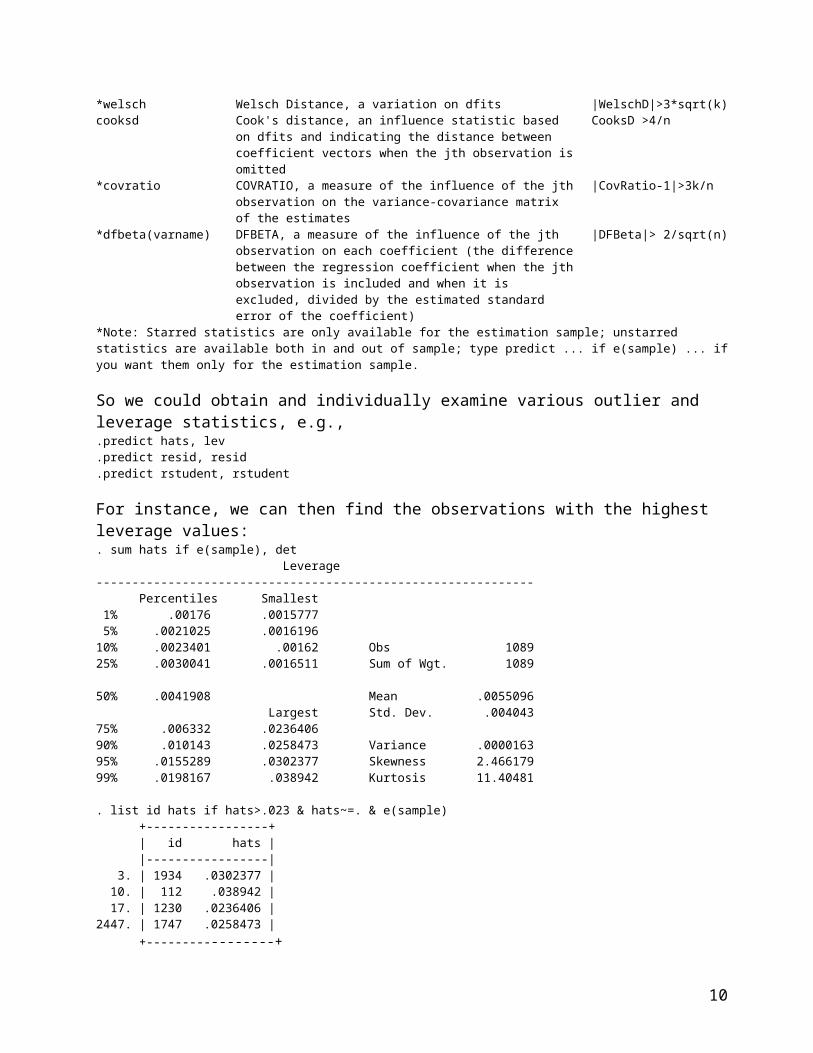
So we could obtain and individually examine various outlier and leverage statistics, e.g.,.predict hats, lev.predict resid, resid.predict rstudent, rstudent
For instance, we can then find the observations with the highest leverage values:. sum hats if e(sample), det Leverage------------------------------------------------------------- Percentiles Smallest 1% .00176 .0015777 5% .0021025 .001619610% .0023401 .00162 Obs 108925% .0030041 .0016511 Sum of Wgt. 1089
50% .0041908 Mean .0055096 Largest Std. Dev. .00404375% .006332 .023640690% .010143 .0258473 Variance .000016395% .0155289 .0302377 Skewness 2.46617999% .0198167 .038942 Kurtosis 11.40481
. list id hats if hats>.023 & hats~=. & e(sample) +-----------------+ | id hats | |-----------------| 3. | 1934 .0302377 | 10. | 112 .038942 | 17. | 1230 .0236406 |2447. | 1747 .0258473 | +-----------------+
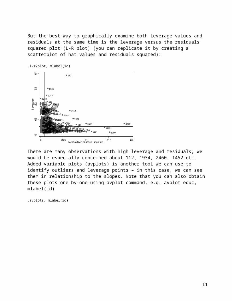
But the best way to graphically examine both leverage values and residuals at the same time is the leverage versus the residuals squared plot (L-R plot) (you can replicate it by creating a scatterplot of hat values and residuals squared):
.lvr2plot, mlabel(id)
1934
112
1711594
1230
2156
2235
68
1268
2013
459
2497850
4471699
2638
75114717941457
88815
5 2415
1018
24242196
8052125930
1152
9241982
21882069
1847
1569481266722961347
2516 2718244
2281
1928
2475740
1196
6302673783
352
1683147516152112752
569140369523871673
4602348
1906
1954
246146
970
42
22248397472073
1834
1102
2451243
2556
1395
1884
1059
823840
1164
2402127614971043
2458
246713491985
249119092462
20701356
7552727249021151271
1681258113
633610
671431
11616782250729
442
224122
514
11222681627156213362435
843 2003
2368835
2124
2461299
1448550
2175
2702553824
1684
6221344
20262275126051520391758439
393
1966280
1229
242612581961
892 9601126 11141104
8361608228
2367177220005851205
138217161353
5651542642157
2328415
2508913786
25391427101959184818411354 1977665937
936894789
1626928
2164
1622
2385402
1999
24802377117
323
2411916
2755915491909
906
709
1964
110114091004
1885
1616
2707 1402891
1200
2351
1596
9982669
50
878 1240
16
1057
976
26072238
7971751
2027 2540921365978
1165
2520
214823162700
1136
2225
2579
443
1071
2169
1566
595
17712212
63416871686
2557
1511
1117168984
7902757110696851
506
1120
15581930618 1128749
1912106326002453
1613
1284
30723881672
21711432
945
1163
23332522008
2764
1575
492
2665659
1469215527022194
2034
653
1208
1153
1552251249
1193
152812023865991526
1262152226531515
1512
221311333801157
2089
356
2719
10251140 8221846
2604
2086148240956215233062404
229
53921492052
2382
533624904
877
973
1201
2613
435
1762208820671685
1305
2036
1366243712781072991 5962054
114
2362
876 24772241
5328962159 12185672522215224321887
2763
23452725
22762542
2402488 1547
367
20061795
1971408
1478
10782580
11592446
132826332112
58784
1355
2472803261011132233
269914769502341
25722035
1186
827194824511292
17642009
26841983
213326182335
22631974
570
2639232268
1900
26371094 1426572
4045831068
20621496
972712
855
1952
23472136
281 2481166813671116 61212
358118214720251969830
138519552448 609785980
15511082232
91
1599271260527342660715
2622603
2611
8561664
1451
1142 929 15062427
468
19811679 6548101266
2187
2131177025841192
22
1720690
14252354791
1039
18452185
2752758
196
1535
844
166310862720 10341209 742861298
11212220
198
2019
809 219014302236
1100882
56
13102051
157717252239
26892167
19391242159 23955578932657
7781461
1583
11301710
19901037
297
2765
2436
640
145524131682
115449540121321880
1676416133 2505753
12231054
225
2322
25312438739
275321104072270
14582498
102
1556
1666875
5591077
509
1662104
19514861050
710
1001896796
244483
144545
938
2729
16961468
2007
2166
8161521
21652071
24921882015
1066
1996
969
406
1923
2100399
2481576987
6811997544 15401667 208
516975
26242041796
10444082262
2321
12981832
82364591
1614
268015652032
25991564
27382722
1361134
7381407
934103108016381501
508
2151204319562526
265
5111103588
770
512421
227
1546227417881967
711
23972174
2410
2205249
1316842
503
939
2641
2058
601369
400
7312350
2563 25681563
269 1357260
18289632634660
12561145
571
2704
383
7842726807
1694
1233
426
1274
1231
1530
649
543
23279
1172
18072661902
14821536
2536
1677758 1436135812462655
1567 2122663173
3111753
377
622158719 26022750619
44
1760
1618
6451559813 1220
1591151725602329
586
1946575
354
2394
1549
955 195321182533
10352302578704 11911374
576
655556
174926501724
23661370
535 18031680531
1649
675
1005
1588
1917
14945102357
2059
2065
1181
1752
128217151259
1176
2200845
372
63224421250
4622591
1761
425 1394
2353126
1972
707 1827
1217
1877
100114601882617
2414261 1500214417179401604
294
2336
994
1965326
18731585
1829499
7241169
1654 322
288
457
769
194
636244114706381630
11891586 209211822142
2339
23341390889
2440
2309264918972129
1171
1089
1188
371
1175
22641282288362
14023371631
178
241872 1824683
1838
2197138618102502
2625
18701539
2460
271027282741
25611892
857 883274
2703979
1245
16932737776
113210201541793
235
2457
682
25374272209
2285304 14921082
627
13895810221215
17898622550
686
1971
17792320
231
34113041146
538
498
17002449262321982551143
1811
657
1742
2119 18233732227
3761798
77117915821671840
890
1875
1452
1625714
1491455
6761650687
99
24392791713
22651329
1110 366
24841099
1767
2511
1194
96
1911
1747
12394319761957
24342292
264417192046
602369
480
2361501
1733
205320
6661303
1806
1420
15681096
1449
18042545284
1051
1787
1518
77725661485
21148882040
1534
20961656296
430
2338788
2022
309
1306286276914
958
2061 2060
1049
411
1088500607
96718791400 806
613
612
13
541
2485
1819669
632874361337
1056 524
1932
21401774
16591895
15271488
11611359
179110761709
5221311483
773
527
11743391428
1653 55935
8862083685 282
0.0
1.0
2.0
3.0
4Le
vera
ge
0 .005 .01 .015 .02Normalized residual squared
8

There are many observations with high leverage and residuals; we would be especially concerned about 112, 1934, 2460, 1452 etc. Added variable plots (avplots) is another tool we can use to identify outliers and leverage points – in this case, we can see them in relationship to the slopes. Note that you can also obtain these plots one by one using avplot command, e.g. avplot educ, mlabel(id)
.avplots, mlabel(id)
112
1934
1230
59417112156
2235850
681268
2013
88
794
24971699
447
2415
7511457
4592638
1471
511962196
21881347815
1834
6309302424
1152
2296
2461
2667
352
481
1982
24480578318471569924211212510182069
2516
2462
14035691683228162221242242175247523484610592458
2718
2387
2752
267313491395
695
16734601475740
19281615272725561954
1276
19092070
8393231900
1102
20731497823970211587724461884
6331682035
1795
114
198514511596
2453
1356
2133
24672402976
1575
1885
1243
747
19641355442
840
906
120821871229
835
1284
1200
2362
116
2491
9842036505951758
514
246
67
14781448
19061547270245
2382
755
222425816272490104323284211641260
2368
1305
562
591122
2086
550196625841299
2166
2233
439
16685151116
729203926226812712553
2275
9042633932435824
2270875
45
570
2729
640110441511402633404
1212
599
2755
19711422054
11281762
2765491
1681
1106
92
1562609
14082347
2164
5331113896
2448
1114
21551528
1948
2610238610688431427
11323331258
2026
22
2540
15121522208910041687280562758263716709
1558
1771
27252603
654
565
1353915
2136
105798018412426
2542
1599
2212
1515968
136523677122472876937216777821712669367258026072660
1542
659
195
2388
1622269914322034
1426
1983117
1240
2131
5321511
16781336241158521699131686
1583
2250443122610
1344
2003
16843567891431255720062147238515235961679108
252
1613435
2088
19551367120546820711551
1328
20002432827
2579
1981
1192
298
10782613929
978
1974
797
102550616169732752409972
1382
2522215725202366
120
653
1549
822
3541063
23413802185
58311571664803836
4021608
1506
2488892406
1186
4921153
2395
2354587
2665
1912
223816721469
1764
8941066
1685
14022700
1772
16262112
624
1996
251278540975
111711631430
2335
5162436634
2684
508
1274
1848
909749136
7869982377
2536
2653
960
25991552
891
2152
711
21497911455
567
2757
681
2225271
936
240412984007156426586111019928
17102481
2025
1242
25082213
2351495856
2505
15661676
1716
509
10711770
2480
950
790
809
1482451
2498
2165
14092067
253949
102
112610502734205224272008
307
416
1133
770
146123161577
6
1077
1556880
12012298301486
2763
8101354
1526
1977
84
2492
1969
240
2232855882
1425
665
1218
2560
12781961
270210941366
260526112194
1496
206211302236108618962027
1292
16632657
832159
559
1407
14582268
2600
1266923878
2531
2477
2148118945281166218461213358991
10195391193
1952
1468112091615351374
19827192322
3061476
51
2618
2263
618227620091887
1072
1165
2764
2604
23452707
1999228
57281621
25722241
1100
2753133
1614
91
2437230
1385
9691930
893
1720
1990
2704
27221559
1154
241311361760
543
2158
1262
200717511845
16822019
1034
1881159
557297
131010473915012205
1217
20152563
19651054
690
5881752159
75825911357
12231828
16387105761517262420512680
1037232112311567244422391939195631119612462726
2190
9381080844
1209
2634
11342641
15362438
2526675
1521556
742
21102043
6191946
1176
5861576241011912601316
421955407
212
1039
21511807738
112116491002720
512268914457961588
704
1546225731
2220
153020582118
54416961667
1666
217462441103426197117251923104450326619391256
753
645
1172
660
1591
136917242032963
25335715911259
1747
5751827
1500
902273823971035991694
9341358
204
23272482457
1145
719
124519971631
373
24
326
987
2351032750
682383807
2414
649
1540
2578
627
82
2439
1586
2440228521442200274123941717
1654
10821175
7762065
1089
19671953269179622741220
408
2568
2625
655842
1753
1482
6572100
1897
1700
18752227724
16041715
2460
24926632081677
1803
2611233
1735311618
5111788
227377
2602
194
1215617235063260
1436
364
2655
24491250174918112262
3991564
174281337215631565
1823
535784189223295868670711321877940
1832
2336457
2353
2623
1625
1917602
2197
1171
2442
994
1786838891169
10051194
20591370362
2119
12821394
42519721001
2357
6762882561
2650
366
638
18101389769
538
179
182915821460
2537
1110
2941386
3411873
16931882
2441
455979845
126
2292
23341630
4981329
2264
1789
2434
2309
1541022
158513042129
2649427
636
1491499
179321981188890
7141680
1761
2320
2339
1181167
462
2092
510
25501494
1976
1840
1452
22883761650
25111798
8571911
2484
2337
320274
114643
304214214327101182
22651824
883
2737
19571492
7711239
231
2209
1872
15182502
309
12813902551
1779
1051
501
371
1020888
1713
480
1879687
15392114
18061719
2022
104914066696736918702791470
205
862
2728
2703
1189
322
7771099
1838
1306
411
14851303
607
24852046
96
1534
2566541
2361
1767
43017332862644
1819
6131449276
7882338
1088
2545
1659
11612965001420206020962061914
1568
1400
669
20401804284
17871056806339
1096
13
15271656958
133721404361774
524
612
14886355
287
2083685886
13591895131
527522
19321653
1709
1076
282
1428
1791
1174
935
773
1483
-10
010
2030
e( a
gekd
brn
| X )
-15 -10 -5 0 5 10e( educ | X )
coef = .6158833, se = .05610987, t = 10.98
2591975
25608771298
50904657232821241724
14302292
595
6272236134915172624258424391461135515761004
2395
125011042071376176097621741577
9062198139527221687236611221900619
2449
415
640
1767
1583
46791
60212172083
9842665
260
11402633
27191001111724381455263
70423851631
17492498630710406739
1428
15152144
427
2689
1586
6902641
19661243
1682
14322699
148514861080516
968
2200
176223341556246
219710441896339
1559
1976
1672
2680
1512
1328771823
1681
1353268625832382
2086
2270
158819714001713233815221303404112118481627
2563
1810
1523
2092
224
2034816244
19321153
1733
23942750
150197212582302446
2185
2467
588
232726371840
282
2089134426113651662
1106
27411260
1171
1686913
2212
856
1242
1315962402
2453
13162321
1176
3582727
559
1212888
22051562
524
1885
92
4423358802726
1196769
258
562
116
1154
1407421747
1231
18342704
1274
23678301271
1491
499
156883515582142480
1625
21157122472239754424421807
12921965
17741460
2649266117161664
2505
15362133
4071685416
1063362
244427101567
14261215714
1969587
164912391672667
609
2712368
58
2566
1071
179
601347167816792725
1306
940
889
64921
2220205912591717
1099498
1492
9391770
18291582
23291676108632
843
2550
1604
645
501
783
1540
254218975502354
2166
2644
8101408
20966762623719
1982440
2537
51226001068
2350
366
617
2414439
136
211807
1476
9371841
286
1653135421401103
1957
1803
24801374
24095351266202524
373
2239265
8402233298
1213
2347426
2000
309
168
2035
2285950
25261823
8781752
225133
1819
2511533
1082
1654
909288
21572522
6817902872491
967686
1427687
1939
1758
1240
82
145881322092536
1276
1977
1526
11131793
7492561204319517952757
2621005
13864021608
707
1054
252842
1892
2477
322
1389
22819
2758561668
1547
2046
613
8961667
994
148325208271615
114
148
1663
2765341
1521
1613
436
1566
2058
87522881964515
1425
16842167930
776
55
857
809
1436
1072
15421996
685886
1677
1956311
532
213122682320
2755
9551732669
2065
84
599970
306
17091873742
892
12231591
14701157
45
212
1879517872061
1967
934998
21882553
1693
128
2026
945
326
1136557
1791
1511
15991771197
1827
15526181449
2232
240
1114
2448778
1329178
19462707
2540
22751882
2657
2110
492
2060
2516364
13578931246
2413
2603
850
1152
1500
14022700
15631182855
2155
2264
1089
2492
17791788806
1256
2165
26551494
1828
6755651282
235
159
883
2156
2114
654
695
902
1468
13041116
2502
1034
53125782580367
862
715
2653
1990
87610351409
83
936669
556281
297
1700100214924371528
27182602
4622462
2159145120671527
1056
2441
1382
5691638
2703
923
273872422271875
183225722599
204
1358
284
1948
607
1789
11302613
2164
890
2539
2551
2388
2158189523532461
2151
671310
2339
2112777
1824
9352692070
575
665
2387
653
929
2484
2194
1798
11102737
2545
9871715
21879141431789
2265
622
276
248
1218
23862610265064
978
68349
24151305
1174
2345
1506
2729
1020
758
6
11422512
2262
773
2241
96
2309
154
9608822434
500
1596
11322451
2190
1191180610310252015711
17961022
2424
19172171
105117251694
11261870
1845
938104
1659212527281585263422632475
1022196
43
9632720401208
12781101
1974198312301683
511
18461696
738
1262
1076
2460
2054
408
729
891
2341
1872
753
1912
522
21477881761
16801656634
2684
1448217513692039
2118
973
5941385
2568
2607
9282152140063815658611134
1043135920888242491478
11001128
636107718842660
8392027
2129
228
2276273420524552238
120
1551
274
1161
2119
457
1145510
1953
1172427105018771955
14886821751171926632007
296
16509151673399
275
1132508222413561847
2008
97913672490
2432208
491
1535
1096
2435
2213
24971710
63
845
307
2337
1997
1146
2032
1630
20132250
2702
1961
23511469822
58510885911402579
2022
2322
2485
1753
655
1094
23331804
279120920511930
275220091086
894
1764
1838
991
1192
1981
27531057
2136
13372625495143
194
1189
2377
6591366731
803
83659
1403
12202274
1475
126
2036
231
304
2605
78418872073177228010191037
1497
10492533
1457
9589801390
2069
567
2481
1626
380188
204010782100
2361
22961205770
572539
2411511954
1284
12992404
1720
1336624666
2618
3691169
231615461539371
245270
24261200
481
740
2235
785
612
11932488253111337961445
7866331182148660190920032357
1482
11652410
1120916882006
755570
2362
294
1811
1711
1564
19282348
794
2673
68
1163
216912291999
1569
2764
1181
1985
1622
1471924
751
1159805
9114961201
797
11021420
229196
1666
116419721018
2763
2062122
1982
383
610
4591268
460
815
26381934
12451518
174722411
1616
1549
10594432557323243624571911
571
354
2019
1575
969844
541
1370
1233508
576
430
2556
42
1394
506167092611503
1534425205
1066
2458
527
509
393
1172112
1530
5144421039
1952
1742
99
161419061186
320372
1452
16992225538118813
356
35211941618
26041175586468543
2336227377
447
1923435
-10
010
20e(
age
kdbr
n | X
)
0 .5 1e( born | X )
coef = 1.6790781, se = .57575994, t = 2.92
7101117221461411
6191577275065723271760115346
229226991432
2092
2334232926412220830249823381911233524615561627506
524
406
627
131135323501512
2034
2124913168615221662
1492
2059
587810225
1063
1355
843
559
2096
544
2212
2051354
2089
807906
976244
287
8802726
714527
393
180726492025
255015881161426
550153684210721526
1977
1136
2409
2491
8355352382
4989091521617
2704
2140198
512306
2000
32322682757
1054
1747
1575
749
5011906
400
1803
1566
889
17911494
783
742
845761213
117613888
211184119711281957
18321068827
2703
16672242225
806436
462
2354
2526
2623
1215
2110240
2232
1452
2026
1240
1458
2572998
855
115726049701182
1885
930
1389695
255325781427159685886
923
55284
27001402
2413
21562275
893
1823532
2131955
936
189715422241
2653
10352262
1034
51374
23452551
2718
1725
2516
366
21942440
5386652621892
1511
1824
320102012181262
1382
96798718702387
2264599
17982112
2285
57517712652263
6
261324922603
511
2451
929103
1056
960
156587621252512
1506654500978
1656
1789
1694
1917
562758
1278
1751
9
2545
10763772272388
46851022762336
1872
2765
607
1715
249
112
399
13292164154
2309
891
2424
2265
1974
1022
1191
2152
26631838882195313697581488729
2490
1585
274675
208
2171
522824
2250
1700556
2118
21472634
120
788
279
22271875
724
1189
1961
2702200720091997
1146
1305
2337
1175
1094
543
2129
2196
7841110401134
2032
296
2051
24341923
1659
10771887822275224971475136622741220
1535
2119958
5942013260591510883041630572
457280
1037
2460
20401337
4352533
1161
12082481
567
1086123014971057
2136
3713802175740242611652003
1299
1133
2235
1564
1482
980
1457
23572411
755
7861941546
36929419281159
2764
142091
20362673
24101471
16661496633
19851164805196
1711
1018882348162220621811
1982
26381934
176727192689
1428
24383761001161619322174125026651121690112222367399045712198844
771
123314301576
1733
12431724
1682
25572019259113491517262413444434220831303
1681
13702385
17491672
704282
239410041044969358260
196625601848232813955831687823268
427
1258
1394
1328
62
975
1104
239550261112982584856791
10594151515246727222144151860
184097220711245
1568145515624078161140263318961292
2436152396887724021460148610802200425
1485
21421678
747
171324495952632556
541
1969
1154
2680244450317161762
442710
2644430
219759623972442
1810
126024391583
1476
1271649261107126002711685155927271664211519761540
266114831770
32213162563126640417746308131365
26671099
2637940
5881491499
258
4218781653
719
1501
167
769
984645232116709
1172
2239
9391242339
121724801106
2086
640
21
602
1171
4801679
2367
6872368
1586
2185
1549
123123015341631950
921952
2457
24771212
22051039
840
108
2472712632
1436
155816841939
82
220919004397901103
1615
179
2566147041615671239
2505
2046362173426
51616771005
16041347
15821829
1625
354
17172725
25222157148
133609
2458
286
1306562
1563
994
1787253715301066
2542676
2707
4021608364618
1676707
509
1709
9452270
937
862
85712592741265519672288
24142520
178822811407
58
122314082061
2437
1819
508
252127618821186
179351516181613
9342366
2058
24461699
514
288892
15911779
1649
2602
100
2347281
6132453
15523722043
2320
13862060
17585572561
669
93525021895
533
1282
883
1274
1663442
2159
341
2511492
2233298196514091113715902
1425
1431686
773
1196118812562067896
21211742133
21492669
1873
297
2065
269
3111956
1990
8092539
14491358
204
2728
1152
1693
273826503561668
2737914
2755
2657
1742
1996
194613101599
309
21882353
24
373
1468
531
96
753
49
161418345691304
136
642481696
1654
1082
1796
12462166
1752
653
21902540
135727201527
1114
2448195
1385
197
831783672580
2339
1827
1761
1680
565890
938
2165
1828
681
112621551846
1547
201516820351500
244120702151253621671130
850776
104352
228
78918454081638102515281043
276
11011879
99
1795247567
2568
963111614001948
1964875
114
20275869287781806
2484
634
26842158
1912
7772341
326273420522610238616832462
21142224
109645
6831673
1089
20392427973
2415
19301142114584522381847188423563
2008738
1194
11325081983
1100
2088140
447
1650
1132102
1877
307
135943
2213
1551
839
135617531804636
991
2351
19552607
14486382435
1209259924322054136726601451
45514695918611171719
126
218710192579
1128
1439791051
894
176424611050
2312729
2377
6222322585
711
1192
1981
275320691596803836
1390511710539
491
612
655
17722100
2361275
261824851403
1336731
2333207314781539
1626
18811932404659
245
231679614454951078624682
1720
2296214811812051120916
2022481
19547852488666596602625
11811999
270
10492531
1169
190920061569681163924
794
7701201751
2292169
1284
57019721200
122
79727636101229
1102
383
459
2362
4601268815
-20
-10
010
20e(
age
kdbr
n | X
)
-1 -.5 0 .5e( sex | X )
coef = -2.2178232, se = .30436248, t = -7.29
19321483
322
183811361832
753
8132329243742
8621262
1233
1563
17511494
1385
2703
2728
60
26892719
1930
6121952
1725
1470
9352220
462
1436
2604
1618
773
13443641420
26551696
2572
1039
1189
176727071121
1314762241
2350189515651159510358
1733
1680
1761
1428
225
1788
1684
2262
618
2602
37722726111072
26442281174
784
17384440739914311678100
2600
2345
282
17911266
306878
1677
13942477
2438
1292687287
2720425
1787
9451615
1181511
2811370146010012263
91
1564
1096
8061870
1656
227623941846
1906
5722268
2159
2009
7711882
1043
1666
51
1999
2618
1568
279
1887
1969
1445796923
958284
991
1401019
669
22501303
1779
1709
1967
5396491165
2444842
1540
2046
22242209690119316531521223921422650
82
845269571
2764742
9161120830271019397102027
2110
2490
2019249
1796856
1020
12582502
2750810
126
2663
1354208
408
200313361716128
1492
2568
1804
1071
96
2061
1673
1977
1526
17702194206921481181539
2480
1400849502551
1681
1076807
790
1753
240
223263883
2190
855
148
914
209612212231282
9381562
610
2361
719
739271222527372059665376
100521251164
1218
1616
1475
695
210014091848
1172
2442206712432578
25392397969
1278
23271953
49
8431209
202513902665112650374014881682
747
1182
18722040
857
2060245
994
167215661847
1099
6
7152702
196124911186
1699
10941220227427342052
1824
11172427
19281592008
231
840934
64
2026
1366
307
371
2467
2605987184024021685
1054
103155211012757
755204
13582335583
928
1452
393
2451
2149248
1482294
143
1154
9402508506
2213
20151136452351
936
23161044
55716649021153909
447
7492288
27381145
297
2357
2051274
21562718
156913102682174
587
972460
998
1035
17981496
2426
823233626611018
2387
924
266716084021591
11461037
939
104
2653
892197212716237219972802062
524
1201
235316944927073042292115
205
1328
634
2684
960441471
2557
1063276325222157
247511332337
1034
1530
27001402
25202404
891
96318451774
575
527
21521256
1650
191711031122
2752
426
2481
2112
1990
2377
1912
1250
1966816
2092
25121332556
167
383
500
443439
2238
11572413
5911749
196
653
24091469215151356
7512385
2550
567894
1764
187722818152341
1506
17725351523188
13698931923
1626
596
2673704
25531884
97045962468
2275
131
468
24351025
20002007
1188
1382
7852032
1679824
2638
430
544
108
43621988272320803
836973
2058
2039
481
2533
2522083786
632116316131260356
5506601667
2235
569
2339
120
126826132488
929
2368805
1100
978
822
427
1551
1720
1683197424322140
7142579729
12762338
541
27532727380
1981
1192261
1491
499
435
6172088522
1955
1078260
1367
1152
890
20701793
16869132516
2296
1316
1527
286
15761534512421
2236
21181819
1713
198207312057891985
1403839
6132649
531
1982
258166293016271896
480
233413591807685886
797
14681449
1497
25451803
1299
212
1304269914321604
1213
276
2147
1810
731
5862034498
55961924241515
769296
514
968709162497
21515
179
538
1426
18291582
1337
16631365
2537
2144
22220023226362367
411
788
1056
1080
738712247214582657
1386
1486195455
2566
1240
9551806
2264
341
832013
937
2043
1873
2641151726242006
532
2131
1789
1693
1088
1102509
1909
6767941511
1717
154
230910041059
1719
1022
194624411687246288
585
501
2669
15851349
26802561
146115461535
2212
1395
1536
15771983
2542123914853672580
2129
1911
232111302436
154220651934
12312637
1389
1556117
14252526
1567134717581715
4161353
2414
455155824582726
666979272588023881191
1599
588
211
362
260724982660
1242
1956311369
1630638
2169
79167
2505
1512
1841145587612461522
253116761957
2089
2563
1306
320783
442
1762
2411659
565
1430
1066
1448
2171
655
21972492
1106
2188809
92
1104
1357415
182826331140
1171
1724
609
2165
2540
16381501882
140826344042205
2347
1161086533
11342395
17711113
1212
2603896461068
654
10288924851427
270
607
2448
1114
2155
1625
43
90410501528
2265
835
178
2410
2722
1948
12592511
238626101077
24842755
15591760758
263197683915861
352
2185
2119
1622406
1976
2441710
1827
1057
2136
1996
1500
11422333495980
1614
2164
2623
2302054
1128
599
2354
2415
207117427772584
491543
686
27041169215858
145785024491132298
20862233
40
1711
1668262
2196
1116
1823
457
1892
562
12292328
570594
2756301583
339
1588
23482462121515181649
633
2292
14071374
25609676571245
59
1305
1659
11611879
243950
8882114
1586
2591
195595
1176
2382
1329
24572741
1897
1945761811
309
6272434
2167
15471654
1082129898477820221175
366776
1700
18752227724
1631
1049
1089
8850810511194
2460
2440
675
228555611101217
99
373
24
975
1752
1549
602
1575
354
1478326
1965
2625400
235
640
516275856
681
1355
906
1274
265
9
682
1362270
8772536976
2453
1964
2133
2765
2124
25991885770
2446
711
8752187
452242035
1682729
1795
114
203632319711451
12081284
190015961200
2166
1230
2362
6222175
1196
2461
112
1834
1747
2366
-10
010
20e(
age
kdbr
n | X
)
-20 0 20 40e( mapres80 | X )
coef = .03319454, se = .01187284, t = 2.8
1117271971026892438112212434613491461266515779041344
168161913951153223669017672174112110018232699143224673919662750
14301627238537683010041672268
1682125812502335
212417602328246735823272498184815761687222058350151726241104
24413531328
15122402155626412329
2034258425911724704406415
747
6571562856152225601515168691323941044
2395260
2198843
877771
972
975
2667
1749
11402633
13557911678
5879681523
10632334
2263062810
2092
1292
16621298
2156
207119322212
595906
23501455229297616162089
1428
27272631260
1896816
1733
1354
21151486
40727221271559225
17621969
11617161303
596627
2491
60
42755020251080
1154
422144
147610712444880544835
271
1583205978326002338
1426
168525816642680
4042200807177013652382211146012662726
1492
44
1526
1977
2409263718401347107225571615180711362397443
840
984
9092368
844
878
649
2083
2000
105915592449
208630611062757
524
21422268201924427492480
2367
25631588571
15369302661
282
16791316
261
1540
198
1521640842
243950615662197
92
4391242
168412337142710
12121810
813224
588
1713
1054
9502239
2649
1568
712247251900
2704
108
421
969150121
2477
84
2550
2185
15581315127196951485
23212611
2096
1841970
790
64540053510689392556940
2644
2281
742
2026
1213827617
411
230123112171370
322
1939
498
2205
1976
2232
240
2725
1240
4991491
416
609
5622505
252221572354167
1803769998127618851482572
2718
2553
25161157
1436
254282
39324361103287
855
211010991586
1494
4021608
1458
117111761394
516
15672707
1631
632
6181667937
1832
133
2526
88914272275687
9454266021731911
1677
1408
515
2270
501
1676
2520923
480
27001402
2387
252197124372131
532
1774
11961604
1542
244622094621005
936
159
1717
1792653
1563
1906
1758224112451281613
1223364
1215
362
21252140503
262324132345
2453
1152
893
892147023471483
425
1407
1625
2703
2578
262
15821829
994
323
1957196721942655
1575
281
1034
1552888
665707
1788
1239
1511
21881259165370916533339
9552046
2537
24141374676
17251518100
1218
1035
1382
21592233
1182599
2566
1699
1389
2741492
20585571113
1262
2262
934
14312366850
20514091771
15912112806
857
1663715
1882
58
862
1791
19522602
2288569
6
20432133
261324582263
298
896
1834
1274
1649
18231897
1306
20672603
286
2669436
2424
1172
2149
15491425
1793
929
112541
24511787
87610399602539
654
2225987288
2492251226525512440
1506430
1668
57597817795941282297
809
1965
2755
9021892
1386
1990
2320
1819
25611256
212
2061
1599284
366
1278576
1824
23882502
2604
17512758561747
1956311
883
341
2070
5111020
49103269265764
1996
2285
2264
2457354
106617092540
1565187022761310
1114
2448
527
204
13581798
653
1972475
1468
2065
2738
88668550925116132765
36725809
686216655514
2164
1694
1385565
753
2490
1946
20601547
1682035
1952155
136
2415
1043
11861530
1696
1873891669
1126967
219083
18467292720265019742497
19172481534
2165219612301246442
16932152
135782450867938
1796
2353
1789
531
1452
2728189516832497892015
2250
681
17951752
152839921712013
510
22827372167
373
2410251828
16731847882
1101171513
1130246219641116935
1654
1082
1827
1304104
114
1948
2536161818452147
1191
2224
1449
2151
1872
120
1680
1761
2663
500
2027
75815001369
1788751953
105696
16381656
309
2339
408928
2752
2309
154
9148901961
2702
2545
18841475208
773
634
2684
1305
2009
1912
238626102039
1174
2341778
675
2441372
1329
27342052
963
2568
2118
10222634
10946072007
776
453565381142556973
8391132427
2265
135618381585
19302158274
2238352401700
4681983107620081527
2235
250819972088822
320
1887
2051
724
18752227
307
144815512213
1077
1100
113413667842435
279118820321879
1145
102
1189
326915
276
2607
1614
2351
1955738377227
99126052801535
447
2461
1089
11462069
6831451
2337
2054
2484
1488180624321400
2660845136721295727881469
1742
22741220235117
1209
2336175314971110
77718772187740522
62221142599
1037
1128
861243412082579
1132
1457
14010191650
1096
1403
1764
894
2481
567
21752119591
2962377
6361596
43272910505851086
2136
1057
1981
11926382426
3801630
457
30425338368035862073
491
2322455
2460
165951
126
1336229627535396399
1299
20031772711
17101804958
2618245543
10881165275
2333
755
1478
481
979
1711
171914313591928
1626
11332319806591471210019231193240424111175
2040
188655
7311051
23161078786
1954
37113376241390
68495
1161
26731205144579611821481564
1482
435
17201120916
11941546
2764
7851159
236123571539
612
20362488
2485
591569805
79491
194
682
751294
270
1909881985
1999
92411641018369633660
1496
24102531
1666
2006
20222348
1181
26251163
1420
666
196
1982
1169162212012062
1284
2169
1268459229570770
1049
1102
122
12001229
797
610193427632638
46018111972815
2362
383
-10
010
2030
e( a
gekd
brn
| X )
-40 -20 0 20 40e( age | X )
coef = .05826431, se = .00992019, t = 5.87
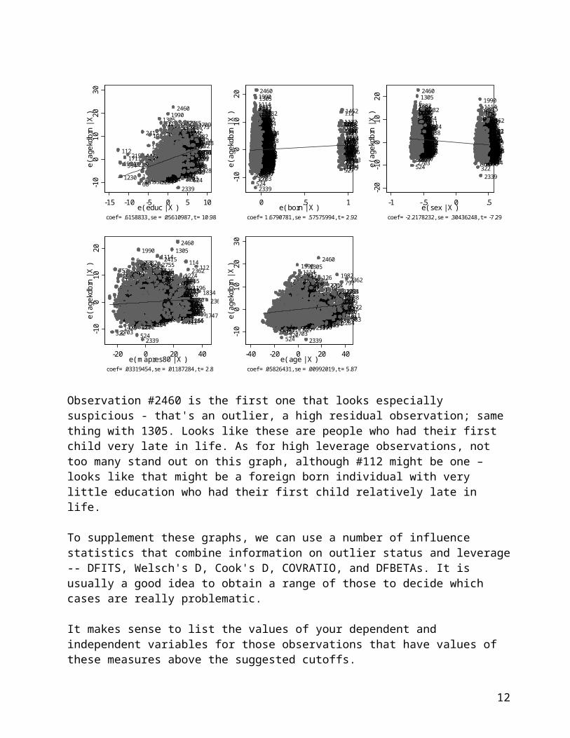
Observation #2460 is the first one that looks especially suspicious - that's an outlier, a high residual observation; same thing with 1305. Looks like these are people who had their first child very late in life. As for high leverage observations, not too many stand out on this graph, although #112 might be one – looks like that might be a foreign born individual with very little education who had their first child relatively late in life.
To supplement these graphs, we can use a number of influence statistics that combine information on outlier status and leverage -- DFITS, Welsch's D, Cook's D, COVRATIO, and DFBETAs. It is usually a good idea to obtain a range of those to decide which cases are really problematic.
It makes sense to list the values of your dependent and independent variables for those observations that have values of these measures above the suggested cutoffs.E.g., we get Cook's D (based on hat values and standardized residuals):. predict cooksd if e(sample), cooksd
9
Don’t forget to specify “if e(sample)” here – Cook’s D is available out of sample as well!NOTE: if you already generated a variable with this name (e.g. cooksd) but want to reuse the name, just use the drop command first: e.g., drop cooksd
Now we list those observations with high Cook's distance. The cutoff is 4/n so in this case, it's 4/1089=.00367309.
. sort cooksd
. list id agekdbrn educ born sex mapres80 age cooksd if cooksd>=4/1089 & cooksd~=. +--------------------------------------------------------------------+ | id agekdbrn educ born sex mapres80 age cooksd | |--------------------------------------------------------------------|1031. | 1394 30 15 no female 28 33 .0036766 |1032. | 63 19 19 yes female 34 64 .003683 |1033. | 2484 37 17 yes female 52 56 .0037003 |1034. | 1906 29 10 no male 23 39 .0037224 |1035. | 994 38 15 yes female 33 41 .003788 | |--------------------------------------------------------------------|1036. | 22 19 12 no male 44 23 .0038182 |1037. | 1402 37 12 yes male 33 42 .0038667 |1038. | 742 36 13 yes male 28 39 .0038726 |1039. | 366 37 17 yes male 66 44 .0041899 |1040. | 2265 39 17 yes male 52 55 .004212 | |--------------------------------------------------------------------|1041. | 2703 16 16 yes male 23 45 .004219 |1042. | 1284 17 12 yes female 64 76 .0043403 |1043. | 2764 35 12 yes male 23 75 .0044005 |1044. | 1114 39 12 yes female 46 46 .0044603 |1045. | 2653 38 12 yes male 32 43 .0044713 | |--------------------------------------------------------------------|1046. | 322 13 16 yes female 20 38 .0044766 |1047. | 352 16 9 no female 44 49 .0045471 |1048. | 1382 39 12 yes male 35 45 .0045595 |1049. | 1990 42 13 yes female 34 46 .0046982 |1050. | 514 16 11 no female 40 42 .0047655 | |--------------------------------------------------------------------|1051. | 1186 30 12 no female 30 44 .0049131 |1052. | 669 37 18 yes female 32 49 .005042 |1053. | 1428 17 20 yes female 32 28 .0052439 |1054. | 753 35 13 yes female 17 51 .0053052 |1055. | 797 34 12 yes female 35 83 .0054951 | |--------------------------------------------------------------------|1056. | 126 38 15 yes female 28 65 .0056446 |1057. | 1824 41 16 yes male 34 49 .0058367 |1058. | 6 40 12 yes male 29 47 .0059349 |1059. | 447 26 6 no female 23 55 .0060603 |1060. | 1549 32 14 no female 66 34 .0061423 | |--------------------------------------------------------------------|1061. | 1066 32 13 no female 47 40 .0062896 |1062. | 612 36 18 yes female 23 73 .0063017 |1063. | 508 18 14 no female 64 40 .0064009 |1064. | 1747 24 17 no male 86 36 .0065845 |1065. | 1189 39 16 yes male 23 62 .0066001 | |--------------------------------------------------------------------|1066. | 773 37 20 yes female 28 54 .0070942 |1067. | 2545 42 18 yes male 46 54 .0072636 |1068. | 1709 38 20 yes female 35 47 .0073801 |1069. | 541 35 18 no female 46 37 .0075467 |1070. | 524 16 19 yes male 42 34 .0075767 | |--------------------------------------------------------------------|1071. | 430 35 18 no female 44 38 .0075794 |
10
1072. | 1194 21 17 no female 66 60 .0079331 |1073. | 435 19 12 no male 36 67 .0079604 |1074. | 1172 33 14 no female 32 39 .0080491 |1075. | 411 21 18 no male 51 30 .0082472 | |--------------------------------------------------------------------|1076. | 1952 31 12 no female 20 40 .0083125 |1077. | 1575 34 12 no male 64 34 .0090088 |1078. | 1934 25 0 yes male 23 89 .009117 |1079. | 1711 27 2 yes male 36 69 .0093139 |1080. | 114 37 12 yes female 66 47 .0096068 | |--------------------------------------------------------------------|1081. | 2156 25 2 yes male 20 33 .0104581 |1082. | 527 22 20 no male 44 43 .0112643 |1083. | 2362 36 12 yes female 64 83 .0117106 |1084. | 1305 44 12 yes male 56 53 .0125958 |1085. | 2415 35 7 yes female 42 48 .0133718 | |--------------------------------------------------------------------|1086. | 1982 37 8 yes male 30 83 .0139673 |1087. | 1452 41 16 no male 36 47 .0191272 |1088. | 2460 50 16 yes male 64 62 .0251248 |1089. | 112 32 2 no male 63 38 .0434919 | +--------------------------------------------------------------------+That's quite a few; the largest Cook’s D belong to observations 112, 2460, and 1452. All of those stood out in graphs as well, so we want to investigate those, but first we might want to examine other indices (e.g. DFITS, COVRATIO, etc.) as well. In the end, we want to identify and further investigate those observations that are consistently problematic across a range of diagnostic tools.
E.g., we can combine the information on high leverage, high studentized residual, and Cook’s D:.scatter hats rstudent [w=cooksd] , mfc(white)
0.0
1.0
2.0
3.0
4Le
vera
ge
-4 -2 0 2 4Studentized residuals
To identify problematic observations, let's replace circles with ID numbers:. scatter hats student [w=cooksd] , mlabel(id)
11
1934
112
1711594
1230
2156
2235
68
1268
2013
459
2497 850
4471699
2638
7511471 7941457
88815
5 2415
1018
24242196
8052125930
1152
9241982
21882069
1847
1569481 266722961347
2516 2718
244
2281
1928
2475740
1196
630 2673783
352
16831475 16152112752
5691403
69523871673
4602348
1906
1954
246146
970
42
2224 8397472073
1834
1102
2451243
2556
1395
1884
1059
823840
1164
24021276
14971043
2458
24671349
198524911909
246220701356
7552727249021151271
1681258113
633610
671431
1161678 2250729
442
224 122
514
11222681627
156213362435
8432003
2368835
2124
2461299
1448550
2175
2702553824
1684
6221344
2026227512605152039 1758439
393
1966280
1229
242612581961
892960 1126 11141104
836 1608228
236717722000 5851205
138217161353
565154264 2157
2328415
2508913786
253914271019
59184818411354 1977665937
936894789
1626928
2164
1622
2385402
1999
24802377117
323
2411916
2755915 491909
906
709
1964
110114091004
1885
1616
2707 1402891
1200
2351
1596
9982669
50
878 1240
16
1057
976
26072238
797
1751
2027 2540921365 978
1165
2520
214823162700
1136
2225
2579
443
1071
2169
1566
595
17712212
6341687 1686
2557
1511
1117 168984
7902757 110696851
506
1120
15581930
618 11287491912
106326002453
1613
1284
30723881672
21711432
945
1163
23332522008
2764
1575
492
2665659
1469215527022194
2034
653
1208
1153
1552251249
1193
1528 1202386599 1526
1262152226531515
1512
22131133 3801157
2089
356
2719
10251140822 1846
2604
2086148
2409 56215233062404
229
539
21492052
2382
533624904
877
973
1201
2613
435
1762208820671685
1305
2036
1366 24371278
10729915962054
114
2362
876 24772241
532896 2159 1218567252221522432
1887
2763
23452725
22762542
2402488 1547
367
20061795
197 1408
1478
10782580
11592446
132826332112
58784
1355
24728032610 1113 2233
2699 14769502341
25722035
1186
827 194824511292
17642009
26841983
213326182335
22631974
570
2639232268
1900
263710941426572
404583 1068
20621496
972712
855
1952
23472136
28124811668 13671116 61212
358118
214720251969
8301385
19552448609785980
15511082232
91
15992712605
27342660715262
2603
2611
8561664
1451
1142929 15062427
468
19811679 6548101266
2187
213117702584
1192
22
1720690
14252354791
1039
18452185
2752758
196
1535
844
1663
10862720 10341209 742861 298
1121 2220
198
2019
809 219014302236
1100882
56
13102051
157717252239
26892167
1939 12421592395557893
2657
7781461
1583
11301710
19901037
297
2765
2436
640
1455 24131682
115449540121321
8801676 416133 2505
7531223
1054225
2322
2531 2438739
2753 21104072270
14582498
102
1556
1666875
5591077
509
1662104
19514861050
710
100 1896
7962444
83
144545
938
2729
16961468
2007
2166
8161521
21652071
2492 1882015
1066
1996
969
406
1923
2100399
2481576 987
6811997544 15401667208
516975
26242041796
10444082262
2321
12981832
82364591
1614
26801565
2032
25991564
27382722
1361134
7381407
934103108016381501
508
2151 204319562526
265
5111103 588
770
512421
227
15462274 17881967
711
23972174
2410
2205249
1316842
503
939
2641
2058
601369
400
7312350
2563 25681563
2691357260
18289632634
660
12561145
571
2704
383
7842726807
1694
1233
426
1274
1231
1530
649
543
23279
1172
18072661902
14821536
2536
1677758 143613581246
26551567 212
2663 173311
1753
377
62 2158 719 26022750619
44
1760
1618
64515598131220
15911517
25602329
586
1946575
354
2394
1549
9551953 21182533
1035230 257870411911374
576
655
556
174926501724
23661370
535 18031680531
1649
675
1005
1588
1917
14945102357
2059
2065
1181
1752
128217151259
1176
2200845
372
632 24421250
4622591
1761
425 1394
2353126
1972
707 1827
1217
1877
10011460 1882617
24142611500 21441717 940 1604
294
2336
994
1965326
18731585
1829499
7241169
1654322
288
457
769
194
636 24411470
6381630
11891586209211822142
2339
23341390889
2440
230926491897
21291171
1089
1188
371
1175
2264 1282288 362
14023371631
178
241872 1824683
1838
2197138618102502
2625
18701539
2460
271027282741
25611892
857883274
2703979
1245
16932737776
1132 10201541793
235
2457
682
25374272209
22853041492 1082
627
138958 10221215
1789862
2550686
1971
17792320
231
34113041146
538
498
17002449262321982551143
1811
657
1742
2119 18233732227
3761798
77117915821671840
890
1875
1452
1625714
1491455
6761650 687
99
2439 2791713
22651329
1110 366
24841099
1767
2511
1194
96
1911
1747
123943 19761957
24342292
26441719 2046
602369
480
2361501
1733
205 320
666
13031806
1420
15681096
1449
18042545284
1051
1787
1518
77725661485
2114 8882040
1534
20961656 296
430
2338788
2022
309
1306286276914
958
2061 2060
1049
411
1088500607
967 18791400 806
613
612
13
541
2485
1819669
63 287436
13371056524
1932
21401774
16591895
15271488
11611359
179110761709
522 1311483
773
527
11743391428
165355935
8862083 685 282
0.0
1.0
2.0
3.0
4Le
vera
ge
-4 -2 0 2 4Studentized residuals
Another set of index measures of influence, DFBETAs, focuses on one regression coefficient at a time. It is a normalized measure of the effect of each specific observation on a regression coefficient, estimated by omitting each observation and comparing the resulting coefficient to the coefficient with that observation included in the data. Positive DFBETA value indicates that an observation increases the value of the coefficient; negative value indicates a decrease in the coefficient due to that observation.
. dfbeta(1676 missing values generated) DFeduc: DFbeta(educ)(1676 missing values generated) DFborn: DFbeta(born)(1676 missing values generated) DFsex: DFbeta(sex)(1676 missing values generated) DFmapres80: DFbeta(mapres80)(1676 missing values generated) DFage: DFbeta(age)
. di 2/sqrt(1089)
.06060606
. scatter DFage DFsex DFborn DFeduc DFmapres80 id, yline(.06 -.06) mlabel(id id id id id)
12
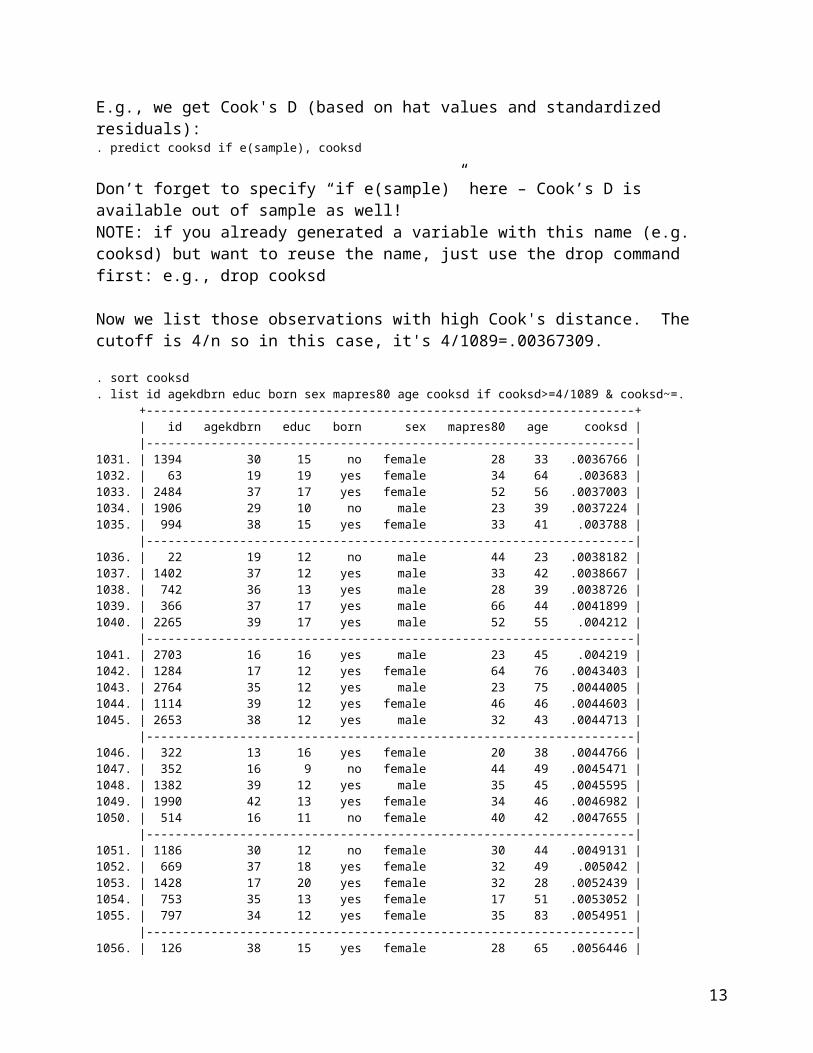
5691316212224404243
4445464950
5155565859
6062
63
646768828384
88
91
92
9699100102103104108112113114116117118120122
126
128131133136140143148154159167168173178179188194195196197198204205208211212224225227228229230
231235240
244245246248249252258260261262263265268269
270
271274275
276279280281282284286287288294296297298304306
307309311320322323326339341352354356358362364366367369371372373376377380
383
393399400402404406407408411415416421425426427430
435
436439442443447
455
457459
460
462468480481491492495498499500501503506508509510511512514515516522
524
527531532533535538539541543544550556557559562565567569570571572575576583585586587588591594595596599602607609610612
613617618619622624
627630632633634636638640645649653654655657
659660665
666
669675676681
682
683685686687690695704707709710
711712714715719724729731738739740742747749751753755
758769770771773776777778783784785786788789790791794
796
797
803805806807809810813815816822823824827830835
836839840842843844845850855856857861862875876877878880882883886888889890891892893894896902904906909913914915916923924928929930934935936937938939940945950955958960963967968969970972973
97597697897998098498799199499810011004100510181019102010221025103410351037103910431044
1049
1050105110541056105710591063106610681071107210761077107810801082108610881089109410961099
11001101
1102
110311041106111011131114111611171120112111221126112811301132113311341136114011421145114611521153115411571159
1161
116311641165
1169
11711172117411751176
1181
1182118611881189
1191119211931194
11961200
1201120512081209121212131215121712181220122312291230123112331239124012421243124512461250125612581259126012621266126812711274127612781282
1284
12921298129913031304
1305
13061310131613281329133613371344134713491353135413551356135713581359136513661367136913701374138213851386138913901394139514001402
1403140714081409
1420
14251426
1427
1428143014311432
143614451448144914511452145514571458146014611468146914701471147514761478148214831485148614881491
149214941496
14971500150115061511
15121515151715181521152215231526152715281530153415351536153915401542154615471549155115521556155815591562156315641565156615671568156915751576157715821583158515861588159115961599160416081613161416151616161816221625
16261627163016311638164916501653165416561659166216631664
1666
166716681672167316761677167816791680
16811682
168316841685168616871693169416961699170017091710
1711
17131715171617171719
172017241725173317421747174917511752175317581760176117621764
17671770177117721774177917871788178917911793179517961798180318041806180718101811
181918231824182718281829183218341838184018411845184618471848187018721873187518771879188218841885188718921895189618971900190619091911191219171923192819301932
1934
19391946194819521953195419551956195719611964196519661967196919711972197419761977
1981
1982
1983198519901996199719992000
20032006200720082009201320152019202220252026202720322034203520362039204020432046205120522054205820592060206120622065206720692070207120732083208620882089
2092
2096210021102112211421152118
2119
212421252129213121332136214021422144214721482149215121522155
2156
2157215821592164216521662167216921712174217521852187218821902194219621972198220022052209221222132220222422252227223222332235223622382239224122502262226322642265226822702274227522762281228522882292229623092316232023212322
232723282329233323342335233623372338233923412345234723482350
23512353235423572361
2362
236623672368237723822385238623872388239423952397240224042409
24102411241324142415242424262427243224342435243624372438243924402441244224442446244824492451245324572458
2460
24612462246724722475247724802481
24842485
2488249024912492249724982502250525082511251225162520252225262531253325362537253925402542254525502551255325562557256025612563256625682572257825792580258425912599260026022603260426052607261026112613261826232624262526332634263726382641264426492650265326552657266026612663266526672669267326802684268926992700270227032704270727102718
271927202722272527262727272827292734273727382741275027522753275527572758
27632764
27655
6
9131621
2224404243444546495051
55565859606263646768
82838488
91
9296
99100102103104108
112
113
114116117118120122
126128131133136
140143148
154159167168173178179188194195196197198204205208211212224225227228229230231235240
244245246248249252258260261262263265268269270271274275
276
279280281282284286
287
288294296
297298304306
307309311320322323326339341
352354356358362364
366
367369371372373376377380383
393399400402404406407408
411
415416421425426427430435
436439442443447
455457459460
462468480481491492495498499
500501503506
508509510
511512514515516
522524527
531
532
533535538539
541
543544550556557559562565567569570571572
575576583585586587588591594595596599602607
609610612613617618619622624
627
630632633634636638640645649
653
654
655657659660665666
669
675676681
682683685686687690695704707709710
711712714715719724729
731738739740
742
747749751753
755
758769770771773776777778783784785786788789790791794796
797
803805806
807809810813815816822823824827830835836839840842843844845850855856857861862875876877878880882
883886888889890
891
892893894896902904906909913914915916923924928929930934935
936
937938939940945950955958960963967968969970972973975
976
978979980984987991
994
99810011004100510181019102010221025
1034
10351037
10391043104410491050105110541056105710591063
1066106810711072107610771078108010821086108810891094
1096
109911001101110211031104110611101113
1114
111611171120112111221126112811301132113311341136114011421145
1146115211531154115711591161116311641165116911711172117411751176
1181118211861188
1189
1191
119211931194
1196120012011205120812091212121312151217
1218
1220122312291230123112331239
1240
12421243124512461250125612581259126012621266126812711274127612781282
1284
12921298129913031304
1305
1306
1310131613281329133613371344134713491353135413551356135713581359136513661367136913701374
1382
13851386
13891390139413951400
1402
14031407140814091420
14251426
142714281430143114321436
1445144814491451
1452
14551457
145814601461146814691470147114751476147814821483148514861488149114921494
1496149715001501
15061511
1512151515171518152115221523152615271528153015341535153615391540
1542
15461547154915511552155615581559156215631564156515661567156815691575
15761577158215831585158615881591159615991604160816131614161516161618162216251626162716301631163816491650165316541656165916621663166416661667166816721673167616771678167916801681168216831684168516861687169316941696169917001709
1710171117131715171617171719172017241725173317421747
1749
1751175217531758176017611762176417671770177117721774177917871788
1789
179117931795179617981803
180418061807181018111819
18231824
1827182818291832183418381840184118451846184718481870
18721873187518771879188218841885188718921895189618971900190619091911
1912
19171923192819301932193419391946194819521953
1954195519561957
1961196419651966196719691971197219741976
1977
1981
1982
19831985
199019961997199920002003
2006200720082009201320152019202220252026202720322034203520362039
204020432046205120522054205820592060206120622065206720692070207120732083208620882089
2092
2096210021102112211421152118
211921242125212921312133
2136214021422144214721482149215121522155
2156
215721582159
2164
2165
2166216721692171217421752185218721882190219421962197219822002205220922122213222022242225222722322233223522362238223922412250
226222632264
2265
226822702274
227522762281228522882292229623092316232023212322
23272328232923332334233523362337
2338
2339
23412345234723482350
2351235323542357
2361
2362
23662367236823772382238523862387
2388
2394239523972402240424092410241124132414
2415
242424262427243224342435243624372438243924402441244224442446244824492451245324572458
2460
2461246224672472247524772480248124842485248824902491
249224972498
2502
2505250825112512251625202522
25262531
2533
25362537
2539
25402542
2545
2550255125532556255725602561256325662568
2572257825792580258425912599260026022603260426052607261026112613261826232624262526332634263726382641264426492650
2653
26552657266026612663
26652667266926732680268426892699
2700
27022703
270427072710
2718
271927202722272527262727272827292734273727382741275027522753
2755275727582763
27642765569
13
1621
22
244042434445464950515556585960626364676882838488919296
99
100102103104108
112
113114116117118120122126128131133136140143148154159167168173178179
188194195196197198204
205
208211212224225
227
228229230231235240244245246248249252258260261262263265268269270271274275276279280281282284286287288294296297298304306307309311
320322323326339341
352
354
356
358362364366367369371372373376377380383
393
399400402404406407408
411
415416421425426427
430
435
436439
442
443
447
455457459460462468480481491492495498499500501503506
508
509
510511512
514
515516522524
527
531532533535538539
541
543
544550556557559562565567569570571
572575576583585586587588591594595596599602607609610612613617618619622624627630632633634636638640645649
653654655657659660665666669675676681682683685686687690695704707709710711712714715719724729731738739740
742747749751753755758769770771773776777778783784785786788789790791794796797803805806807809810813815816822823824827830835836839840842843
844
84585085585685786186287587687787888088288388688888989089189289389489690290490690991391491591692392492892993093493593693793893994094595095595896096396796896997097297397597697897998098498799199499810011004100510181019102010221025103410351037
1039
1043104410491050105110541056105710591063
1066
10681071107210761077107810801082108610881089109410961099110011011102110311041106111011131114111611171120112111221126112811301132113311341136114011421145114611521153115411571159116111631164116511691171
1172
11741175117611811182
1186
11881189119111921193
1194
1196120012011205120812091212121312151217121812201223122912301231
1233
12391240124212431245124612501256125812591260126212661268127112741276127812821284129212981299130313041305130613101316132813291336133713441347134913531354135513561357135813591365136613671369
1370137413821385138613891390
1394
13951400140214031407140814091420142514261427142814301431143214361445144814491451
1452
14551457145814601461146814691470147114751476147814821483148514861488149114921494149614971500150115061511151215151517
1518152115221523152615271528
1530
15341535153615391540154215461547
1549
1551155215561558155915621563156415651566156715681569
1575
1576157715821583158515861588159115961599160416081613
1614
16151616
1618
162216251626162716301631163816491650165316541656165916621663166416661667166816721673167616771678167916801681168216831684168516861687169316941696
16991700170917101711171317151716171717191720172417251733
1742
1747
1749175117521753175817601761176217641767177017711772177417791787178817891791179317951796179818031804180618071810181118191823182418271828182918321834183818401841184518461847184818701872
1873187518771879188218841885188718921895189618971900
1906
19091911
19121917
1923
1928193019321934193919461948
1952
19531954195519561957196119641965196619671969197119721974197619771981198219831985199019961997199920002003200620072008200920132015
2019
202220252026202720322034203520362039204020432046205120522054205820592060206120622065206720692070207120732083208620882089209220962100211021122114211521182119212421252129213121332136214021422144214721482149215121522155215621572158215921642165
21662167216921712174217521852187218821902194219621972198220022052209221222132220222422252227223222332235223622382239224122502262226322642265226822702274227522762281228522882292229623092316232023212322232723282329233323342335
2336
2337233823392341234523472348235023512353235423572361236223662367236823772382238523862387238823942395239724022404240924102411241324142415242424262427243224342435243624372438243924402441244224442446244824492451245324572458246024612462246724722475247724802481248424852488249024912492249724982502
2505250825112512251625202522252625312533253625372539254025422545255025512553
2556
2557256025612563256625682572257825792580258425912599260026022603
2604
26052607261026112613261826232624262526332634263726382641264426492650
26532655265726602661266326652667266926732680268426892699
2700270227032704270727102718271927202722272527262727272827292734273727382741275027522753275527572758276327642765569
1316212224404243444546495051
55
5658596062
63
6467
68
828384
88
9192
96
99100102103104108
112
113
114
116117118120122
126
128131133136140143148154159167168173178179
188194195196197198204
205208211212224225227228229230231235240244
245246248249252258260261262263265268269270271274275276279280281
282
284
286287288294296
297298304306307309311320
322
323326
339341352
354356358362364366367369371372373376377380383393399400402404406407408
411
415416421425426427
430
435436439442443
447
455457459460
462468480481491492495498499
500501
503506508509510511512514515516
522
524527
531532533535538539
541
543544550556557559562565567569570571572575576583585586587588591
594
595596599602607
609610
612
613
617618619622624627630632633634636638640645649653654655657659660665666
669
675676681682683685686687690695704707709710711712714715719724729731738739740742747749751
753
755758769770771
773
776777778783784785786788789790791
794
796797803805806
807809810813815816822823824827830835836839840842843844845850
855856857861862875876877878880882883
886888889890891892893894896902904906909913914915916923924928929930934935936937938939940945950955
958
960963967968969970972973975976978979980984987991
994
998100110041005101810191020102210251034103510371039104310441049105010511054105610571059106310661068107110721076107710781080108210861088
10891094
1096
109911001101110211031104110611101113
1114
1116111711201121112211261128113011321133113411361140114211451146
1152
1153115411571159
11611163116411651169117111721174
117511761181118211861188
1189
11911192119311941196
12001201120512081209121212131215121712181220122312291230123112331239124012421243124512461250125612581259126012621266126812711274127612781282128412921298129913031304
1305
1306
13101316132813291336133713441347134913531354135513561357135813591365136613671369137013741382138513861389139013941395140014021403140714081409
1420
142514261427
1428
14301431143214361445144814491451
1452
1455
1457
14581460146114681469147014711475147614781482148314851486
1488
1491
1492149414961497150015011506151115121515151715181521152215231526152715281530153415351536153915401542154615471549155115521556155815591562156315641565156615671568
1569
15751576157715821583158515861588159115961599160416081613161416151616161816221625
162616271630163116381649165016531654
1656
16591662166316641666166716681672167316761677167816791680168116821683168416851686168716931694169616991700
1709
1710
1711
17131715171617171719172017241725173317421747174917511752175317581760176117621764176717701771177217741779178717881789
179117931795179617981803
18041806180718101811
18191823
1824
1827182818291832183418381840184118451846184718481870
1872
1873
18751877187918821884
18851887189218951896189719001906
19091911191219171923192819301932
1934
193919461948195219531954195519561957196119641965196619671969197119721974197619771981
1982
198319851990199619971999200020032006200720082009201320152019202220252026202720322034203520362039
2040
2043204620512052205420582059
20602061206220652067206920702071207320832086208820892092
2096
2100211021122114211521182119
21242125
2129213121332136214021422144214721482149215121522155
2156
215721582159216421652166216721692171217421752185218721882190219421962197219822002205220922122213222022242225222722322233
2235
22362238223922412250226222632264
2265
226822702274227522762281228522882292229623092316232023212322232723282329233323342335233623372338
2339
23412345234723482350235123532354235723612362
23662367236823772382238523862387
23882394239523972402240424092410241124132414
2415
242424262427243224342435243624372438243924402441244224442446244824492451245324572458246024612462246724722475247724802481
248424852488249024912492
2497
24982502250525082511251225162520252225262531253325362537253925402542
2545
255025512553255625572560256125632566256825722578257925802584259125992600260226032604260526072610261126132618262326242625263326342637
263826412644264926502653265526572660266126632665266726692673268026842689269927002702
2703
270427072710
2718
271927202722272527262727272827292734273727382741275027522753
2755
27572758276327642765
5
6
9
131621222440424344
45
4649
50
5155565859
606263646768828384
8891
92
9699
100102103104108
112
113
114
116117118120122
126
128131133136140143148154159167168173178179188194195196197198
204205208211212
224
225227
228229230231
235240244245246248249252258260261262263265268269270271274275276279280281
282
284286287288294296297298304306307
309311320
322
323326
339341352354356358362364
366
367369371372
373
376377380383393399400402404406407408411415416421425426427430435436439442443447455457459460462468480481491492495498499500501503506
508
509510
511
512514515
516522524527531532533535538539541543544550556557559562565567569570571572575576583585586587588591594
595596599602607609610
612
613617618619622624
627630632633634636638640645649
653
654655657659660665666
669
675676
681
682
683685686687690695704707709710
711
712714715719724
729731738739740
742747749751
753
755758769770771
773
776
777778783784785786788789790791794796797803805806
807809810813815816822823824827830835836839840842843844845850855856857861862875876877878880882883886888889890891892893894896902904906909913914915916923924928929930934935
936937938939940945950955958960963967968969970972973
975976
978979980984987991
99499810011004100510181019
102010221025103410351037103910431044
1049105010511054105610571059106310661068107110721076107710781080108210861088108910941096
109911001101110211031104110611101113
1114
111611171120112111221126112811301132113311341136114011421145114611521153115411571159116111631164116511691171
117211741175
1176
1181118211861188
1189
119111921193
1194
1196
120012011205
1208120912121213121512171218
12201223122912301231123312391240124212431245124612501256125812591260
1262
126612681271
1274
127612781282
1284
12921298129913031304
1305
130613101316132813291336133713441347134913531354
1355135613571358135913651366136713691370137413821385
138613891390139413951400140214031407140814091420
142514261427
1428
143014311432
1436
144514481449145114521455145714581460146114681469147014711475
1476147814821483148514861488149114921494
1496149715001501150615111512151515171518152115221523152615271528153015341535153615391540
15421546
15471549
1551155215561558155915621563156415651566156715681569
1575
15761577158215831585
1586
1588159115961599160416081613161416151616161816221625
16261627163016311638164916501653
165416561659166216631664166616671668167216731676167716781679168016811682168316841685168616871693169416961699
17001709
1710
171117131715171617171719172017241725
17331742
1747
174917511752175317581760176117621764176717701771177217741779178717881789179117931795179617981803180418061807181018111819
1823
1824
1827182818291832
18341838184018411845184618471848187018721873187518771879
18821884188518871892189518961897
19001906190919111912191719231928193019321934193919461948
1952
1953195419551956195719611964
19651966196719691971197219741976
197719811982198319851990
199619971999200020032006200720082009201320152019202220252026202720322034
2035203620392040204320462051205220542058205920602061206220652067206920702071207320832086208820892092209621002110211221142115211821192124
21252129213121332136214021422144214721482149215121522155215621572158215921642165
2166
21672169217121742175
21852187218821902194219621972198220022052209221222132220222422252227
22322233223522362238223922412250
226222632264
226522682270227422752276228122852288229222962309231623202321232223272328232923332334233523362337233823392341234523472348235023512353235423572361
2362
2366236723682377238223852386238723882394239523972402240424092410241124132414
2415
24242426242724322434243524362437243824392440244124422444
2446
244824492451
245324572458
2460
24612462246724722475
2477248024812484248524882490249124922497249825022505250825112512251625202522252625312533
2536
25372539254025422545255025512553255625572560256125632566
256825722578257925802584259125992600
2602
2603260426052607261026112613261826232624262526332634263726382641264426492650
2653
265526572660266126632665266726692673268026842689269927002702
2703
2704270727102718
2719272027222725272627272728
2729
2734273727382741275027522753
2755
2757
275827632764
2765
-.4-.2
0.2
.4
0 1000 2000 3000respondnt id number
Dfbeta age Dfbeta sexDfbeta born Dfbeta educDfbeta mapres80
Observations 112 and 2460 seem to have influence on a number of coefficients; others seem to have effects on specific coefficients, so we need to look into those that have particularly large effects.
Remedies:Once you detected influential data points, you need to decide what to do with them. Typically, non-influential outliers and leverage points do not concern us much, although outliers do increase error variance. We also want to watch out for clusters of outliers, which may suggest an omitted variable. But influential points can have dramatic effects, and we definitely want to investigate those. Once we find them, there is no one clear-cut solution. They should not be ignored, but neither should they be automatically deleted. Typically, the presence of an influential point can mean one of the following:A. Our model is correct, the influential point can be attributed to some kind of measurement errorB. The value of the influential point is observed correctly, but our model is not correct in that it cannot model the influential point well. Possible reasons for that: (a) The relationship between the dependent and the independent variable is not linear in the interval of values that includes the influential point; (b) There is another explanatory variable that can help account for that influential point; (c) The model has heteroskedasticity problems. Unfortunately, often it is not possible to determine which one is the case. But here’s what you can do:
1. You have to investigate what makes these data points unusual —- make sure that you examine their values on all of the variables you use. This will help identify potential data entry errors or might provide other clues as to why these data points are unusual. E.g., we could check #112:
. list agekdbrn educ born sex mapres80 age if id==112 +------------------------------------------------+ | agekdbrn educ born sex mapres80 age | |------------------------------------------------| 10. | 32 2 no male 63 38 | +------------------------------------------------+
13
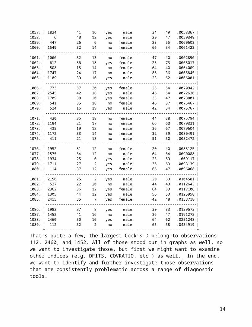
Let’s also get averages for all variables to compare:. sum agekdbrn educ born sex mapres80 age if e(sample) Variable | Obs Mean Std. Dev. Min Max-------------+-------------------------------------------------------- agekdbrn | 1089 23.66483 5.352695 11 50 educ | 1089 13.3168 2.719027 0 20 born | 1089 1.070707 .2564527 1 2 sex | 1089 1.624426 .4844932 1 2 mapres80 | 1089 39.44077 12.95284 17 86 age | 1089 46.1258 15.06822 19 89
2. If you are considering omitting unusual data, you should investigate whether omitting these data points changes the results of your regression model. Try omitting them one by one and compare the coefficients with and without them: are there large changes? Let’s check what happens if we omit #112:. reg agekdbrn educ born sex mapres80 age, beta Source | SS df MS Number of obs = 1089-------------+------------------------------ F( 5, 1083) = 49.10 Model | 5760.17098 5 1152.0342 Prob > F = 0.0000 Residual | 25412.492 1083 23.4649049 R-squared = 0.1848-------------+------------------------------ Adj R-squared = 0.1810 Total | 31172.663 1088 28.6513447 Root MSE = 4.8441------------------------------------------------------------------------------ agekdbrn | Coef. Std. Err. t P>|t| Beta-------------+---------------------------------------------------------------- educ | .6158833 .0561099 10.98 0.000 .3128524 born | 1.679078 .5757599 2.92 0.004 .0804462 sex | -2.217823 .3043625 -7.29 0.000 -.2007438 mapres80 | .0331945 .0118728 2.80 0.005 .0803266 age | .0582643 .0099202 5.87 0.000 .1640182 _cons | 13.27142 1.252294 10.60 0.000 .------------------------------------------------------------------------------. reg agekdbrn educ born sex mapres80 age if id~=112, beta Source | SS df MS Number of obs = 1088-------------+------------------------------ F( 5, 1082) = 50.04 Model | 5841.74787 5 1168.34957 Prob > F = 0.0000 Residual | 25261.3762 1082 23.3469281 R-squared = 0.1878-------------+------------------------------ Adj R-squared = 0.1841 Total | 31103.1241 1087 28.6137296 Root MSE = 4.8319------------------------------------------------------------------------------ agekdbrn | Coef. Std. Err. t P>|t| Beta-------------+---------------------------------------------------------------- educ | .63726 .0565958 11.26 0.000 .3214802 born | 1.515919 .5778803 2.62 0.009 .0722698 sex | -2.187693 .3038273 -7.20 0.000 -.1980863 mapres80 | .030491 .0118905 2.56 0.010 .0737543 age | .0583569 .0098953 5.90 0.000 .1644404 _cons | 13.20334 1.249428 10.57 0.000 .
The actual effect of that observation on the coefficients of educ, mapres80, and born are rather pretty small; for each, beta changes by about 0.01.Also, try omitting the most persistent influential points as a group and examine the effects. If there are large changes in coefficients, you might use that to justify omitting a few (but only very few) observations from the model – but you will also have to explain what is so special about these cases.
14
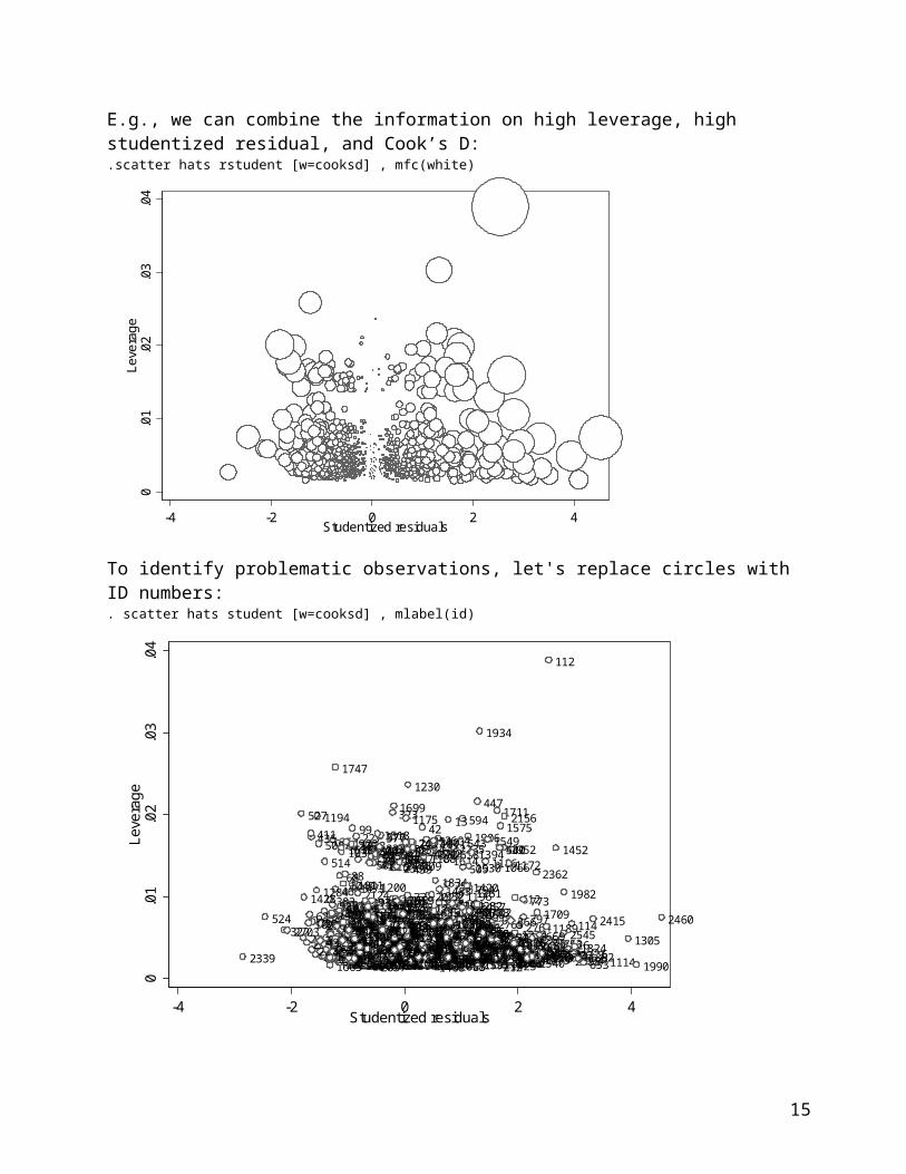
3. To reduce the incidence of high leverage points, consider transforming skewed variables and/or topcoding/bottomcoding variables to bring univariate outliers closer to the rest of the distribution (e.g. coding incomes of >$100,000 to $100,000 so that these high values do not stand out), like we did when we discussed data screening (and if that was done at that stage, it reduces the chances that problems emerge in multivariate context).
4. If unusual data come in clusters, you may have to introduce another variable to control for their unusualness, or you might want to deal with them in a separate regression model.
5. Robust regression is another option when one observes substantial problems with influential data. The Stata rreg command performs a robust regression using iteratively reweighted least squares, i.e., assigning a weight to each observation with higher weights given to better behaved observations, while extremely unusual data can have their weights set to zero so that they are not included in the analysis at all.
. rreg agekdbrn educ born sex mapres80 age, gen(wt)Robust regression Number of obs = 1089 F( 5, 1083) = 52.34 Prob > F = 0.0000------------------------------------------------------------------------------ agekdbrn | Coef. Std. Err. t P>|t| [95% Conf. Interval]-------------+---------------------------------------------------------------- educ | .6518023 .0539119 12.09 0.000 .5460186 .7575859 born | 1.792079 .5532063 3.24 0.001 .7066014 2.877556 sex | -2.012778 .29244 -6.88 0.000 -2.586591 -1.438965 mapres80 | .0275798 .0114078 2.42 0.016 .005196 .0499637 age | .0522715 .0095316 5.48 0.000 .033569 .070974 _cons | 12.34444 1.203239 10.26 0.000 9.983493 14.70538------------------------------------------------------------------------------
. sum wt, det Robust Regression Weight------------------------------------------------------------- Percentiles Smallest 1% .2138941 0 5% .5965052 .000736310% .7419349 .0035576 Obs 108925% .8782627 .0726816 Sum of Wgt. 1089
50% .9564363 Mean .9001565 Largest Std. Dev. .151333775% .988214 .999999890% .9983087 .9999999 Variance .022901995% .9996306 1 Skewness -2.92681499% .9999847 1 Kurtosis 12.98754
Comparing the robust regression results with the OLS results on the previous page, we see that even though there are a few small differences, the coefficients, standard errors, and p-values are quite similar. Despite the minor problems with influential data that we observed while doing our diagnostics, the robust regression analysis yielded quite similar results, suggesting that these problems are indeed minor. If the results of OLS and robust regression were substantially different, we would need to further investigate what problems in our OLS model caused the difference. If it is impossible to resolve such problems, then the robust regression results should be viewed as more trustworthy.
15
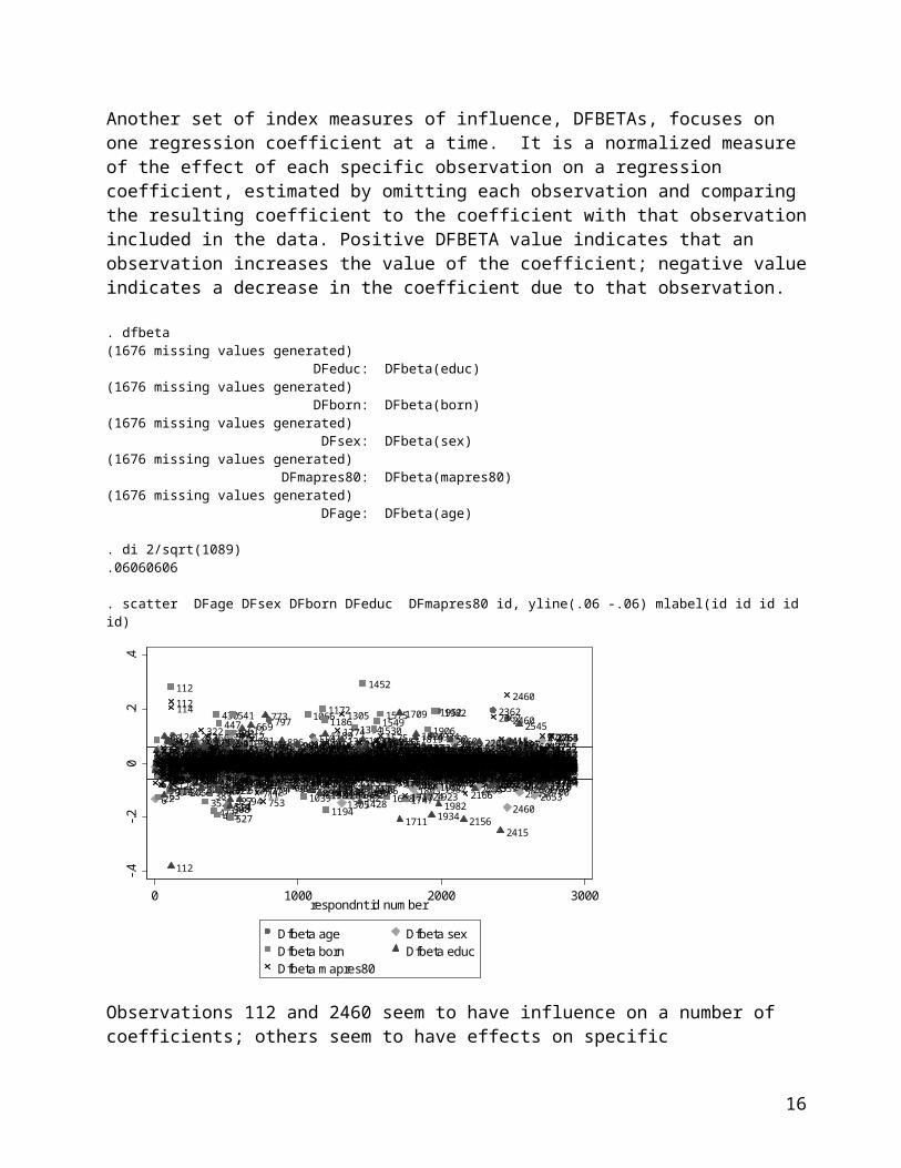
4. Additivity.
First and foremost, we should always use our theory insights to consider the need for interactions. We can have interactions between dummies (or sets of dummies), a dummy (or a set of dummies) and a continuous variable, or two continuous variables. To avoid multicollinearity problems, you should code your dummies 0/1 and mean-center those continuous variables that are involved in interaction terms.
. gen sexd=sex-1
. gen bornd=born-1(6 missing values generated)
. for var age educ mapres80: sum X \ gen Xmean=X-r(mean)-> sum age Variable | Obs Mean Std. Dev. Min Max-------------+-------------------------------------------------------- age | 2751 46.28281 17.37049 18 89-> gen agemean=age-r(mean)(14 missing values generated)
-> sum educ Variable | Obs Mean Std. Dev. Min Max-------------+-------------------------------------------------------- educ | 2753 13.36397 2.973924 0 20-> gen educmean=educ-r(mean)(12 missing values generated)
-> sum mapres80 Variable | Obs Mean Std. Dev. Min Max-------------+-------------------------------------------------------- mapres80 | 1619 40.96912 13.63189 17 86-> gen mapres80mean=mapres80-r(mean)(1146 missing values generated)
A user-written program “fitint” helps find statistically significant two-way interactions, so it can be used as a diagnostic tool.
. net search fitintClick on: fitint from http://fmwww.bc.edu/RePEc/bocode/f
. fitint reg agekdbrn bornd sexd agemean educmean mapres80mean, twoway(bornd sexd agemean educmean mapres80mean) factor(bornd sexd) Source | SS df MS Number of obs = 1089-------------+------------------------------ F( 15, 1073) = 17.65 Model | 6169.67284 15 411.311523 Prob > F = 0.0000 Residual | 25002.9902 1073 23.301948 R-squared = 0.1979-------------+------------------------------ Adj R-squared = 0.1867 Total | 31172.663 1088 28.6513447 Root MSE = 4.8272------------------------------------------------------------------------------ agekdbrn | Coef. Std. Err. t P>|t| [95% Conf. Interval]-------------+---------------------------------------------------------------- _Ibornd_1 | 1.710533 .9779923 1.75 0.081 -.2084614 3.629527 _Isexd_1 | -2.21852 .3179507 -6.98 0.000 -2.842395 -1.594644 agemean | .0587138 .0171439 3.42 0.001 .0250744 .0923532 educmean | .4551926 .0888308 5.12 0.000 .2808908 .6294943mapres80mean | .033156 .0203674 1.63 0.104 -.0068085 .0731205 _Ibornd_1 | (dropped) _Isexd_1 | (dropped)_IborXsex_~1 | .1211157 1.271076 0.10 0.924 -2.372961 2.615193
16

_Ibornd_1 | (dropped) agemean | (dropped)_IborXagem~1 | .0048469 .0568729 0.09 0.932 -.1067477 .1164415 _Ibornd_1 | (dropped) educmean | (dropped)_IborXeduc~1 | -.2922046 .210566 -1.39 0.166 -.7053724 .1209631 _Ibornd_1 | (dropped)mapres80mean | (dropped)_IborXmapr~1 | .0046759 .0414082 0.11 0.910 -.0765743 .0859261 _Isexd_1 | (dropped)_IsexXagem~1 | -.0031427 .0207363 -0.15 0.880 -.043831 .0375455 _Isexd_1 | (dropped)_IsexXeduc~1 | .391932 .1146716 3.42 0.001 .1669259 .6169381 _Isexd_1 | (dropped)_IsexXmapr~1 | -.0005186 .024932 -0.02 0.983 -.0494397 .0484024 __13_6 | -.0038885 .0038209 -1.02 0.309 -.0113858 .0036088 __14_6 | .0004487 .0008266 0.54 0.587 -.0011732 .0020706 __15_6 | .0033919 .0044236 0.77 0.443 -.005288 .0120717 _cons | 24.98069 .2579745 96.83 0.000 24.4745 25.48688------------------------------------------------------------------------------------------------------------------------------------------------------Fitting and testing any interactions and any main effects not includedin interaction terms using the ratio of the mean square error of eachterm and the residual mean square error to obtain an F ratio statistic------------------------------------------------------------------------Model summaryNumber of observations used in estimation: 1089Regression command: regressDependent variable: agekdbrnResidual MSE: 23.30degrees of freedom: 1073------------------------------------------------------------------------ Term | Mean square F ratio df1 df2 P>F-------------------+---------------------------------------------------- i.bornd*i.sexd | 0.21 0.01 1 1073 0.9241 i.bornd*agemean | 0.17 0.01 1 1073 0.9321 i.bornd*educmean | 44.87 1.93 1 1073 0.1655 i.bornd*mapres80mean| 0.30 0.01 1 1073 0.9101 i.sexd*agemean | 0.54 0.02 1 1073 0.8796 i.sexd*educmean | 272.21 11.68 1 1073 0.0007 i.sexd*mapres80mean| 0.01 0.00 1 1073 0.9834 agemean*educmean | 24.13 1.04 1 1073 0.3091 agemean*mapres80mean| 6.87 0.29 1 1073 0.5874 educmean*mapres80mean| 13.70 0.59 1 1073 0.4434------------------------------------------------------------------------It appears that when all twoway interactions are tested simultaneously, the only one that is statistically significant is sex by education. We could also check each two-way interaction separately to make sure we did not miss anything by testing all simultaneously:
. for X in var bornd sexd agemean educmean mapres80mean: for Y in var bornd sexd agemean educmean mapres80mean: fitint reg agekdbrn bornd sexd agemean educmean mapres80mean, twoway(Y X) factor(bornd sexd)[output omitted]
Note that you should always include main effect variables in addition to the interaction, because the interaction term can only be interpreted together with that main effect. Further, if you want to explore three-way interactions, the model should also include all possible two-way interactions in addition to main terms. For example:. gen bornsex=bornd*sexd(6 missing values generated)
17
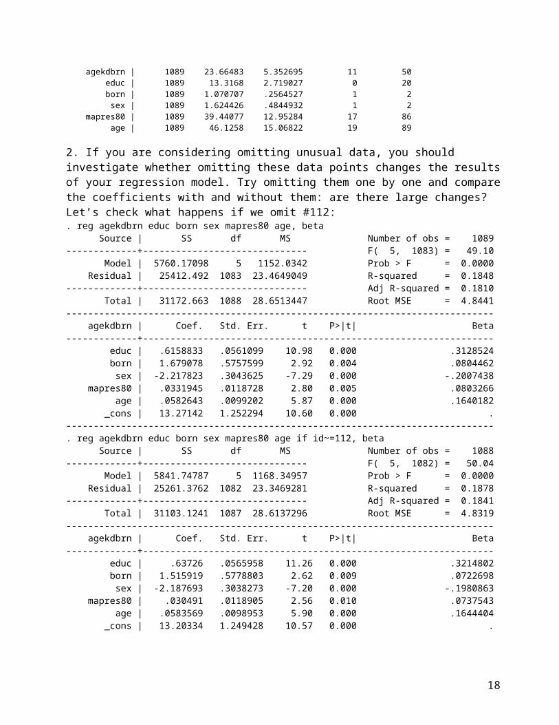
. gen borneduc=bornd*educmean(13 missing values generated). gen educsex=educmean*sexd(12 missing values generated). gen educsexborn=educmean*sexd*bornd(13 missing values generated). xi: reg agekdbrn bornd sexd agemean educmean mapres80mean bornsex borneduc educsex educsexborn Source | SS df MS Number of obs = 1089-------------+------------------------------ F( 9, 1079) = 29.48 Model | 6152.90509 9 683.656121 Prob > F = 0.0000 Residual | 25019.7579 1079 23.1879128 R-squared = 0.1974-------------+------------------------------ Adj R-squared = 0.1907 Total | 31172.663 1088 28.6513447 Root MSE = 4.8154------------------------------------------------------------------------------ agekdbrn | Coef. Std. Err. t P>|t| [95% Conf. Interval]-------------+---------------------------------------------------------------- bornd | 1.779615 .9740461 1.83 0.068 -.131624 3.690854 sexd | -2.220267 .3134215 -7.08 0.000 -2.835252 -1.605282 agemean | .0594442 .0098793 6.02 0.000 .0400593 .078829 educmean | .4461687 .0831105 5.37 0.000 .2830922 .6092451mapres80mean | .0324834 .0118427 2.74 0.006 .0092461 .0557208 bornsex | .0946345 1.204318 0.08 0.937 -2.268437 2.457706 borneduc | -.4745646 .2819971 -1.68 0.093 -1.027889 .0787601 educsex | .3621368 .1124932 3.22 0.001 .1414065 .5828671 educsexborn | .4750623 .3902632 1.22 0.224 -.2906985 1.240823 _cons | 25.00961 .2479526 100.86 0.000 24.52309 25.49614-------------+----------------------------------------------------------------
But we’ll focus on two-way interactions for now, and in order to explore how to interpret them, we’ll review 4 examples: (1) an interaction of two dichotomous variables; (2) an interaction of a dummy variable and a continuous variable; (3) an interaction of a set of dummy variables and a continuous variable; (4) an interaction of two continuous variables.
Example 1: Two dichotomous variables
. reg agekdbrn educ bornd##sexd mapres80 age Source | SS df MS Number of obs = 1089-------------+------------------------------ F( 6, 1082) = 40.91 Model | 5764.17997 6 960.696662 Prob > F = 0.0000 Residual | 25408.483 1082 23.4828863 R-squared = 0.1849-------------+------------------------------ Adj R-squared = 0.1804 Total | 31172.663 1088 28.6513447 Root MSE = 4.8459------------------------------------------------------------------------------ agekdbrn | Coef. Std. Err. t P>|t| [95% Conf. Interval]-------------+---------------------------------------------------------------- educ | .6165377 .0561537 10.98 0.000 .5063552 .7267202 1.bornd | 1.358118 .9670434 1.40 0.160 -.5393752 3.25561 1.sexd | -2.251548 .3152298 -7.14 0.000 -2.870079 -1.633017 | bornd#sexd | 1 1 | .4964787 1.201596 0.41 0.680 -1.861244 2.854201 | mapres80 | .0333659 .0118846 2.81 0.005 .0100464 .0566855 age | .0584314 .0099322 5.88 0.000 .0389428 .07792 _cons | 12.73045 .9671152 13.16 0.000 10.83281 14.62808------------------------------------------------------------------------------The interaction is not statistically significant, but let’s suppose it would be. Then we can first interpret the two main effects: the foreign born men have children 1.4 years later than the native born men, and the native born women have children 2.3 years earlier than the native born men.
18
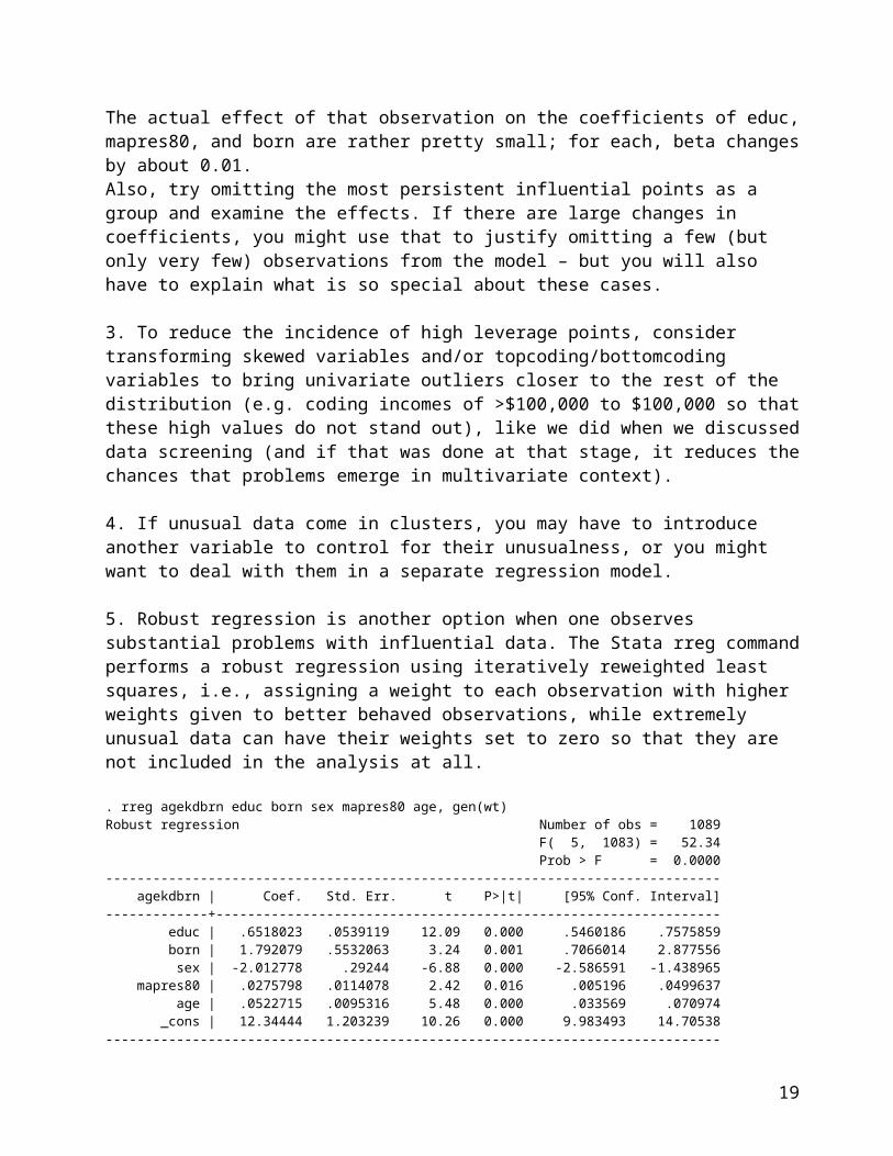
To interpret the interaction term, we need to focus on one variable as our main variable and the other will be used as a moderator. We can do it both ways.
Nativity status as the main variable:The effect of being foreign born is 1.4 for men (i.e., the foreign born men have children 1.4 years later than the native born men), but for women, it is 1.4+0.5=1.9 (that is, the foreign born women have children 1.9 years later than the native born women).
Gender as the main variable:The effect of gender is -2.3 for the native born (i.e., the native born women have children 2.3 years earlier than the native born men), but for the foreign born, it is -2.3 +.5=-1.8 (that is, the foreign born women have children 1.8 years earlier than the foreign born men).
The only time when we would use both main effects and an interaction is when we wanted to compare across gender and nativity status at the same time: that is, the foreign born women have children 0.4 of a year earlier than the native born men: 1.4-2.3+0.5=-0.4
Although it doesn’t make sense to examine an interaction of two dummy variables graphically, we can use “adjust” command to help us interpret this interaction:
. xi: qui reg agekdbrn educ i.bornd*sexd mapres80 age
. adjust educ mapres80 age if e(sample), by(sexd bornd)------------------------------------------------------------------------------- Dependent variable: agekdbrn Command: regress Variables left as is: _Ibornd_1, _IborXsexd_1 Covariates set to mean: educ = 13.316804, mapres80 = 39.440773, age = 46.125805-------------------------------------------------------------------------------------------------------------- | bornd sexd | 0 1----------+----------------- 0 | 24.9519 26.31 1 | 22.7004 24.555---------------------------- Key: Linear Prediction
These are the predicted values of agekdbrn given average values of education, age, and mother’s occupational prestige.
Example 2: A dummy variable and a continuous variable
. reg agekdbrn bornd##c.educmean sexd mapres80 age Source | SS df MS Number of obs = 1089-------------+------------------------------ F( 6, 1082) = 41.17 Model | 5793.5421 6 965.590349 Prob > F = 0.0000 Residual | 25379.1209 1082 23.4557494 R-squared = 0.1859-------------+------------------------------ Adj R-squared = 0.1813 Total | 31172.663 1088 28.6513447 Root MSE = 4.8431---------------------------------------------------------------------------------- agekdbrn | Coef. Std. Err. t P>|t| [95% Conf. Interval]-----------------+---------------------------------------------------------------- 1.bornd | 1.716336 .5764944 2.98 0.003 .585162 2.847509 educmean | .6352486 .058401 10.88 0.000 .5206565 .7498407 |
19
bornd#c.educmean | 1 | -.2323323 .194782 -1.19 0.233 -.6145255 .1498609 | sexd | -2.229199 .3044525 -7.32 0.000 -2.826583 -1.631814 mapres80 | .0334778 .0118729 2.82 0.005 .0101813 .0567743 age | .0587405 .0099263 5.92 0.000 .0392636 .0782175 _cons | 20.93833 .7498733 27.92 0.000 19.46696 22.4097----------------------------------------------------------------------------------Again, no significant interaction, but for practice, we’ll interpret the results.
Education as the main variable, nativity status as the moderator:Among the native born individuals, a one year increase in education is associated with a 0.6 of a year increase in the age of having kids. Among the foreign born individuals, a one year increase in education is associated with a (.63-.23)=0.4 of a year increase in the age of having kids.
Nativity status as the main variable, education as the moderator:Among those with average education (13.4 years), the foreign born have kids 1.7 years later than the native born. Among those with education one unit above average (14.4 years), the foreign born have kids 1.5 years later than the native born (1.7+1*(-0.2)). Among those with education one unit below average (12.4 years), the foreign born have kids 1.9 years later than the native born (1.7 + (-1*(-0.2))). We could also look at those whose education is 4 years below average (9.4 years); for them, the foreign born have kids 2.5 years later than the native born (1.7 + (-4*(-0.2))).
We could estimate this model in a different way to see separately the effects of education in the native born and the foreign born groups; that will also allow us to see if the effect is significant in each of the groups:
. gen educfb=educmean*bornd(13 missing values generated). gen educnb=educmean(12 missing values generated). replace educnb=0 if bornd==1(256 real changes made)
. reg agekdbrn bornd educfb educnb sexd mapres80 age Source | SS df MS Number of obs = 1089-------------+------------------------------ F( 6, 1082) = 41.17 Model | 5793.5421 6 965.590349 Prob > F = 0.0000 Residual | 25379.1209 1082 23.4557494 R-squared = 0.1859-------------+------------------------------ Adj R-squared = 0.1813 Total | 31172.663 1088 28.6513447 Root MSE = 4.8431------------------------------------------------------------------------------ agekdbrn | Coef. Std. Err. t P>|t| [95% Conf. Interval]-------------+---------------------------------------------------------------- bornd | 1.716336 .5764944 2.98 0.003 .585162 2.847509 educfb | .4029163 .1871522 2.15 0.032 .0356939 .7701387 educnb | .6352486 .058401 10.88 0.000 .5206565 .7498407 sexd | -2.229199 .3044525 -7.32 0.000 -2.826583 -1.631814 mapres80 | .0334778 .0118729 2.82 0.005 .0101813 .0567743 age | .0587405 .0099263 5.92 0.000 .0392636 .0782175 _cons | 20.93833 .7498733 27.92 0.000 19.46696 22.4097------------------------------------------------------------------------------
This way we can see that the effect of education is significant in both groups. Finally, we can again examine this interaction graphically. . adjust sexd mapres80 age if e(sample), gen(pred1)
20
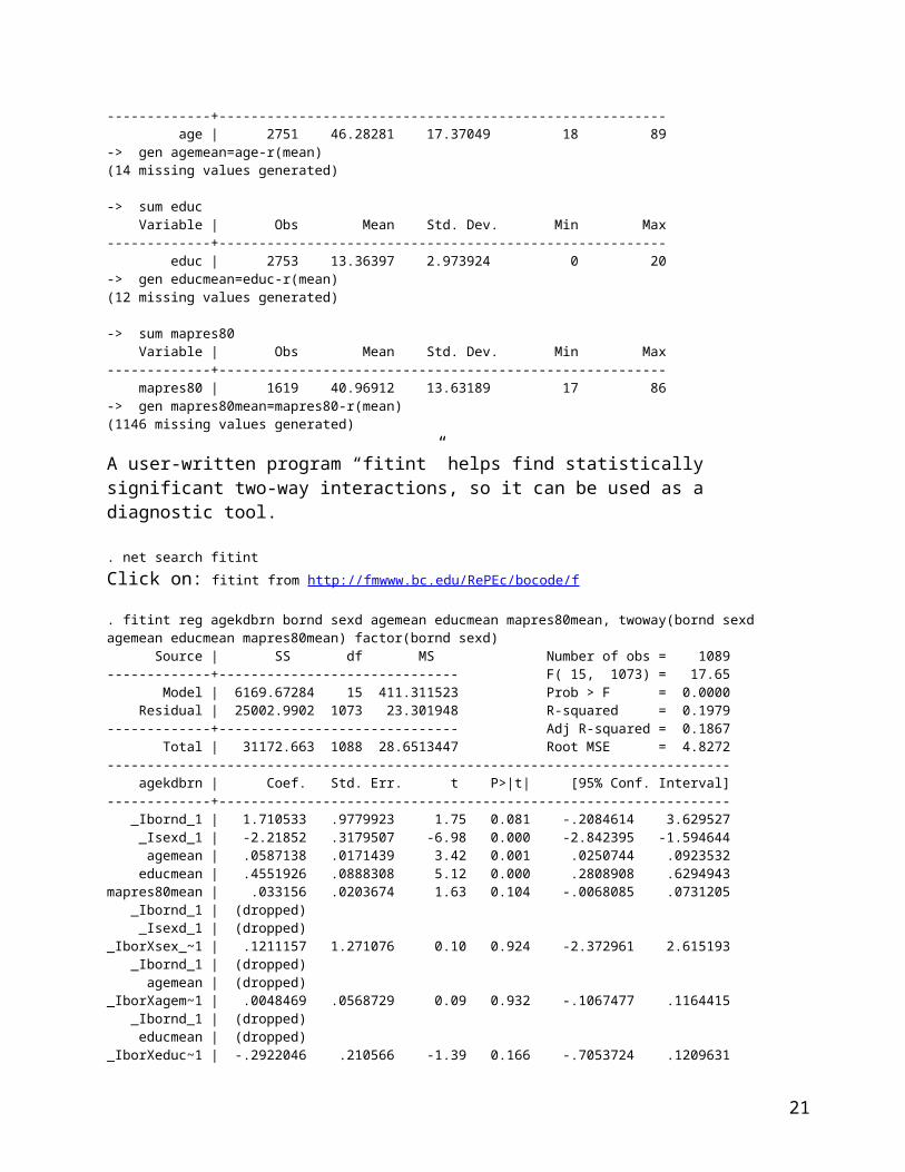
---------------------------------------------------------------------------------- Dependent variable: agekdbrn Command: regress Created variable: pred1 Variables left as is: bornd, educfb, educnb Covariates set to mean: sexd = .62442607, mapres80 = 39.440773, age = 46.125805-------------------------------------------------------------------------------------------------------- All | xb----------+----------- | 23.6648---------------------- Key: xb = Linear Prediction
. twoway (line pred1 educ if bornd==0, sort color(red) legend(label(1 "native born"))) (line pred1 educ if bornd==1, sort color(blue) legend(label(2 "foreign born")) ytitle("Respondent’s Age When 1st Child Was Born"))
1520
2530
Res
pond
ent’s
Age
Whe
n 1s
t Chi
ld W
as B
orn
0 5 10 15 20highest year of school completed
native born foreign born
Alternatively, we could split pred1 into two variables (or if needed more):.separate pred1, by(bornd)
This would generate two variables, pred10 and pred11, which we can graph:.line pred10 pred11 educ, lcolor(red blue) sort
1520
2530
0 5 10 15 20highest year of school completed
pred1, bornd == 0 pred1, bornd == 1
Example 3: A set of dummy variables and a continuous variable
21
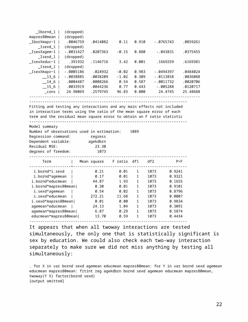
. reg agekdbrn bornd marital##c.educmean sexd mapres80 age
Source | SS df MS Number of obs = 1089-------------+------------------------------ F( 13, 1075) = 21.96 Model | 6540.34346 13 503.103343 Prob > F = 0.0000 Residual | 24632.3195 1075 22.9137856 R-squared = 0.2098-------------+------------------------------ Adj R-squared = 0.2003 Total | 31172.663 1088 28.6513447 Root MSE = 4.7868
------------------------------------------------------------------------------------ agekdbrn | Coef. Std. Err. t P>|t| [95% Conf. Interval]-------------------+---------------------------------------------------------------- bornd | 1.536577 .5729824 2.68 0.007 .4122865 2.660868 | marital | widowed | -.8946254 .626208 -1.43 0.153 -2.123354 .3341031 divorced | -.9166076 .3889825 -2.36 0.019 -1.679859 -.1533567 separated | -1.944692 .7095625 -2.74 0.006 -3.336977 -.5524077 never married | -2.55648 .5380556 -4.75 0.000 -3.612238 -1.500722 | educmean | .6467199 .0727279 8.89 0.000 .504015 .7894247 |marital#c.educmean | widowed | -.3294696 .167311 -1.97 0.049 -.6577629 -.0011764 divorced | .0213546 .151949 0.14 0.888 -.2767956 .3195049 separated | -.0935184 .2455722 -0.38 0.703 -.5753736 .3883368 never married | -.527267 .2268917 -2.32 0.020 -.9724677 -.0820662 | sexd | -2.028997 .3066702 -6.62 0.000 -2.630737 -1.427257 mapres80 | .0292701 .0118022 2.48 0.013 .0061121 .0524282 age | .0435388 .0117499 3.71 0.000 .0204835 .0665942 _cons | 22.24782 .8245124 26.98 0.000 20.62999 23.86566------------------------------------------------------------------------------------ To test whether the set of interactions is jointly significant:. mat list e(b)
e(b)[1,16] 1b. 2. 3. 4. 5. bornd marital marital marital marital maritaly1 1.5365772 0 -.8946254 -.91660762 -1.9446921 -2.5564798
1b.marital# 2.marital# 3.marital# 4.marital# 5.marital# educmean co.educmean c.educmean c.educmean c.educmean c.educmeany1 .64671988 0 -.32946962 .02135465 -.09351841 -.52726698
sexd mapres80 age _consy1 -2.0289968 .02927015 .04353882 22.247823
. test 2.marital#c.educmean 3.marital#c.educmean 4.marital#c.educmean 5.marital#c.educmean
( 1) 2.marital#c.educmean = 0 ( 2) 3.marital#c.educmean = 0 ( 3) 4.marital#c.educmean = 0 ( 4) 5.marital#c.educmean = 0
F( 4, 1075) = 2.22 Prob > F = 0.0653
We cannot reject the null hypothesis, so we conclude that jointly these interaction effects are not statistically significant (they do not add significantly to the amount of variance explained by the
22
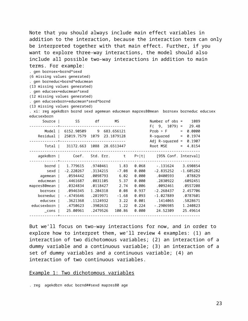
model; although it is possible that with fewer groups, the overall significance test would change). If we were to explore these interaction terms, however, we would want to get the estimates of separate slopes of education by marital status:
. tab marital, gen(mardummy) marital | status | Freq. Percent Cum.--------------+----------------------------------- married | 1,269 45.90 45.90 widowed | 247 8.93 54.83 divorced | 445 16.09 70.92 separated | 96 3.47 74.39never married | 708 25.61 100.00--------------+----------------------------------- Total | 2,765 100.00
. for num 1/5: gen educmarX=educmean*mardummyX-> gen educmar1=educmean*mardummy1(12 missing values generated)-> gen educmar2=educmean*mardummy2(12 missing values generated)-> gen educmar3=educmean*mardummy3(12 missing values generated)-> gen educmar4=educmean*mardummy4(12 missing values generated)-> gen educmar5=educmean*mardummy5(12 missing values generated)
. reg agekdbrn bornd i.marital educmar1-educmar5 sexd mapres80 age Source | SS df MS Number of obs = 1089-------------+------------------------------ F( 13, 1075) = 21.96 Model | 6540.34346 13 503.103343 Prob > F = 0.0000 Residual | 24632.3195 1075 22.9137856 R-squared = 0.2098-------------+------------------------------ Adj R-squared = 0.2003 Total | 31172.663 1088 28.6513447 Root MSE = 4.7868-------------------------------------------------------------------------------- agekdbrn | Coef. Std. Err. t P>|t| [95% Conf. Interval]---------------+---------------------------------------------------------------- bornd | 1.536577 .5729824 2.68 0.007 .4122865 2.660868 | marital | widowed | -.8946254 .626208 -1.43 0.153 -2.123354 .3341031 divorced | -.9166076 .3889825 -2.36 0.019 -1.679859 -.1533567 separated | -1.944692 .7095625 -2.74 0.006 -3.336977 -.5524077never married | -2.55648 .5380556 -4.75 0.000 -3.612238 -1.500722 | educmar1 | .6467199 .0727279 8.89 0.000 .504015 .7894247 educmar2 | .3172503 .1522423 2.08 0.037 .0185245 .615976 educmar3 | .6680745 .1348759 4.95 0.000 .4034246 .9327244 educmar4 | .5532015 .2360602 2.34 0.019 .0900105 1.016392 educmar5 | .1194529 .2155296 0.55 0.580 -.3034536 .5423594 sexd | -2.028997 .3066702 -6.62 0.000 -2.630737 -1.427257 mapres80 | .0292701 .0118022 2.48 0.013 .0061121 .0524282 age | .0435388 .0117499 3.71 0.000 .0204835 .0665942 _cons | 22.24782 .8245124 26.98 0.000 20.62999 23.86566--------------------------------------------------------------------------------It appears that education has a statistically significant effect on age of parenthood in all groups except for the never married.
23

Example 4: Two continuous variables
Both variables should be mean centered: . reg agekdbrn bornd c.educmean##c.agemean sexd mapres80 Source | SS df MS Number of obs = 1089-------------+------------------------------ F( 6, 1082) = 41.24 Model | 5801.57307 6 966.928846 Prob > F = 0.0000 Residual | 25371.0899 1082 23.4483271 R-squared = 0.1861-------------+------------------------------ Adj R-squared = 0.1816 Total | 31172.663 1088 28.6513447 Root MSE = 4.8423-------------------------------------------------------------------------------------- agekdbrn | Coef. Std. Err. t P>|t| [95% Conf. Interval]---------------------+---------------------------------------------------------------- bornd | 1.679599 .5755567 2.92 0.004 .5502651 2.808932 educmean | .6362385 .0581443 10.94 0.000 .5221503 .7503268 agemean | .054804 .0102529 5.35 0.000 .0346862 .0749219 |c.educmean#c.agemean | -.0045353 .0034131 -1.33 0.184 -.0112324 .0021618 | sexd | -2.232587 .3044578 -7.33 0.000 -2.829982 -1.635193 mapres80 | .0335181 .0118711 2.82 0.005 .010225 .0568111 _cons | 23.64786 .52946 44.66 0.000 22.60897 24.68674-------------------------------------------------------------------------------------- The interaction term is not significant. But if it were, to interpret it, we would pick one variable that’s primary and the other one will serve as the moderator variable. E.g. if education is primary:For agemean=0 (age at its mean, 46 y.o.), the effect of education is educmean coefficient, .6362385For agemean=20 (age is at mean+20, i.e. 66 y.o.), the effect of education is . di .6362385 + 20*-.0045353.5455325For agemean=-20 (age=26 y.o.), the effect of education is. di .6362385 - 20*-.0045353.7269445
We can do the same thing graphically -- focus on one of the continuous variables and then graph it at various levels of the other one. E.g., we’ll see how the effect of education varies by age: . gen educage=educmean*agemean(24 missing values generated)
. qui reg agekdbrn bornd educmean agemean eudcage sexd mapres80
. qui adjust bornd sexd mapres80 if e(sample), gen(pred2)
. twoway (line pred2 educ if age==30, sort color(red) legend(label(1 "30 years old"))) (line pred2 educ if age==40, sort color(blue) legend(label(2 "40 years old"))) (line pred2 educ if age==50, sort color(green) legend(label(3 "50 years old"))) (line pred2 educ if age==60, sort color(lime) legend(label(4 "60 years old")) ytitle("Respondent’s Age When 1st Child Was Born"))
24
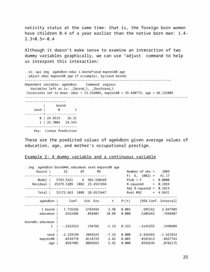
1520
2530
Res
pond
ent’s
Age
Whe
n 1s
t Chi
ld W
as B
orn
0 5 10 15 20highest year of school completed
30 years old 40 years old50 years old 60 years old
Here we can see that the higher one’s age, the later they had their first child, but the effect of education becomes a little bit smaller with age (e.g. with age, the intercept becomes larger but the slope of education becomes smaller).We could have done it other way around – graph how agekdbrn is related to age for educational levels of, say, educ=10, 12, 14, 16, and 20. There is also a user-written command that allows to automatically generate such a graph for three values – mean, mean+sd, mean-sd:
. net search sslopeClick on: sslope from http://fmwww.bc.edu/RePEc/bocode/s
. sslope agekdbrn bornd educmean sexd mapres80 agemean educage, i(educmean agemean educage) graph Source | SS df MS Number of obs = 1089-------------+------------------------------ F( 6, 1082) = 41.24 Model | 5801.57308 6 966.928846 Prob > F = 0.0000 Residual | 25371.0899 1082 23.4483271 R-squared = 0.1861-------------+------------------------------ Adj R-squared = 0.1816 Total | 31172.663 1088 28.6513447 Root MSE = 4.8423------------------------------------------------------------------------------ agekdbrn | Coef. Std. Err. t P>|t| [95% Conf. Interval]-------------+---------------------------------------------------------------- bornd | 1.679599 .5755567 2.92 0.004 .5502651 2.808932 educmean | .6362385 .0581443 10.94 0.000 .5221503 .7503268 sexd | -2.232587 .3044578 -7.33 0.000 -2.829982 -1.635193 mapres80 | .0335181 .0118711 2.82 0.005 .010225 .0568111 agemean | .054804 .0102529 5.35 0.000 .0346862 .0749219 educage | -.0045353 .0034131 -1.33 0.184 -.0112324 .0021618 _cons | 23.64786 .52946 44.66 0.000 22.60897 24.68674------------------------------------------------------------------ Simple slope of agekdbrn on educmean at agemean +/- 1sd ------------------------------------------------------------------ agemean | Coef. Std. Err. t P>|t|------------+----------------------------------------------------- High | .5678996 .066709 8.51 0.000 Mean | .6362385 .0581443 10.94 0.000 Low | .7045775 .0871861 8.08 0.000------------+-----------------------------------------------------
25

1020
3040
50ag
ekdb
rn
-15 -10 -5 0 5educmean
r's age when 1st child born agemean+1sdagemean mean agemean-1sd
Note that this gives us significance tests for the slope estimates at three levels of the moderator variable. If we reverse how we list the two main effect variables in the i() option of this command, we get:. sslope agekdbrn bornd educmean sexd mapres80 agemean educage, i(agemean educmean educage) graph------------------------------------------------------------------ Simple slope of agekdbrn on agemean at educmean +/- 1sd ------------------------------------------------------------------ educmean | Coef. Std. Err. t P>|t|------------+----------------------------------------------------- High | .0424724 .0154784 2.74 0.006 Mean | .054804 .0102529 5.35 0.000 Low | .0671357 .0119546 5.62 0.000------------+-----------------------------------------------------
1020
3040
50ag
ekdb
rn
-20 0 20 40agemean
r's age when 1st child born educmean+1sdeducmean mean educmean-1sd
Finally, let’s consider a more complicated case when we have a curvilinear relationship of age with agekdbrn and an interaction between age and education; we will right away create interaction terms to be able to use adjust command for graphs:. gen agemean2=agemean^2(14 missing values generated). gen agemean3=agemean^3(14 missing values generated). gen educage2=educmean*agemean2(24 missing values generated)
26
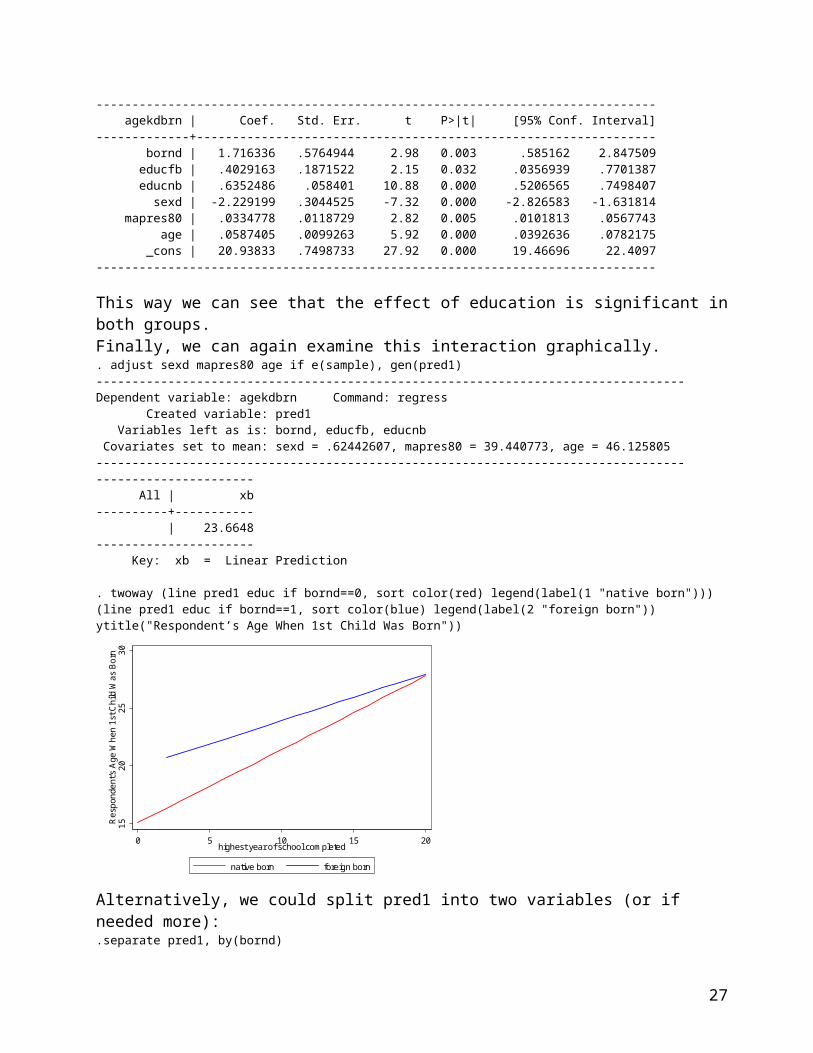
. gen educage3=educmean*agemean3(24 missing values generated). reg agekdbrn bornd sexd mapres80 educmean agemean agemean2 agemean3 educage educage2 educage3 Source | SS df MS Number of obs = 1089-------------+------------------------------ F( 10, 1078) = 35.55 Model | 7731.43912 10 773.143912 Prob > F = 0.0000 Residual | 23441.2239 1078 21.7451056 R-squared = 0.2480-------------+------------------------------ Adj R-squared = 0.2410 Total | 31172.663 1088 28.6513447 Root MSE = 4.6632------------------------------------------------------------------------------ agekdbrn | Coef. Std. Err. t P>|t| [95% Conf. Interval]-------------+---------------------------------------------------------------- bornd | 1.278985 .556004 2.30 0.022 .1880122 2.369958 sexd | -2.113086 .2941837 -7.18 0.000 -2.690323 -1.535848 mapres80 | .0355671 .0114369 3.11 0.002 .0131259 .0580082 educmean | .7185734 .0759774 9.46 0.000 .569493 .8676538 agemean | -.0445573 .0182216 -2.45 0.015 -.080311 -.0088036 agemean2 | -.0064784 .0007326 -8.84 0.000 -.0079158 -.005041 agemean3 | .0002514 .0000327 7.69 0.000 .0001873 .0003155 educage | -.0001007 .005545 -0.02 0.986 -.010981 .0107796 educage2 | -.0008988 .0003225 -2.79 0.005 -.0015315 -.0002661 educage3 | .0000198 9.75e-06 2.03 0.042 6.87e-07 .000039 _cons | 24.53094 .5244201 46.78 0.000 23.50194 25.55994------------------------------------------------------------------------------Indeed, significant interactions with the squared term and the cubed term.. qui adjust bornd sexd mapres80 if e(sample), gen(pred3). twoway (line pred3 age if educ==12, sort color(red) legend(label(1 "12 years of education"))) (line pred3 age if educ==14, sort color(blue) legend(label(2 "14 years of education"))) (line pred3 age if educ==16, sort color(green) legend(label(3 "16 years of education"))) (line pred3 age if educ==20, sort color(lime) legend(label(4 "20 years of education")) ytitle("Respondent’s Age When 1st Child Was Born"))
1520
2530
Res
pond
ent’s
Age
Whe
n 1s
t Chi
ld W
as B
orn
20 40 60 80 100age of respondent
12 years of education 14 years of education16 years of education 20 years of education
5. Multicollinearity
Our real life concern about the multicollinearity is that independent variables are highly (but not perfectly) correlated. Need to distinguish from perfect multicollinearity -- two or more independent variables are linearly related – in practice, this usually happens only if we make a mistake in including the variables; Stata will resolve this by omitting one of those variables and will tell you it did it. It can also happen when the number of variables exceeds the number of observations.
27
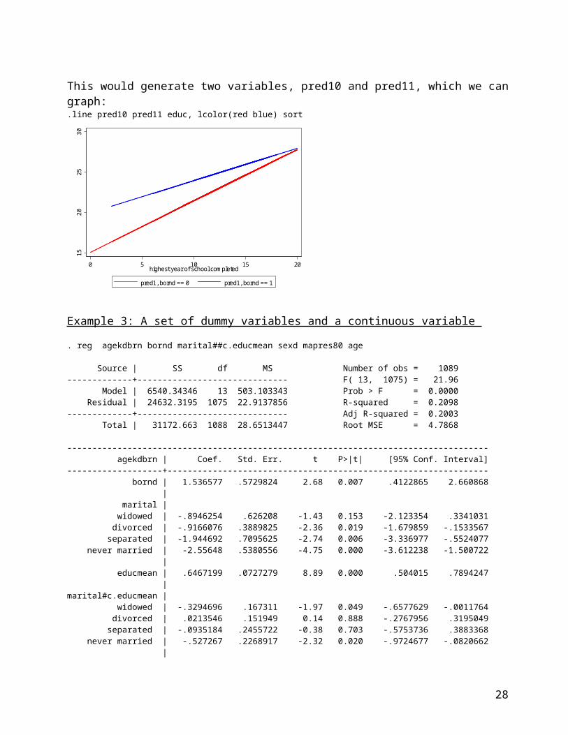
Perfect multicollinearity violates regression assumptions -- no unique solution for regression coefficients.
High, but not perfect, multicollinearity is what we most commonly deal with. High multicollinearity does not explicitly violate the regression assumptions - it is not a problem if we use regression only for prediction (and therefore are only interested in predicted values of Y our model generates). But it is a problem when we want to use regression for explanation (which is typically the case in social sciences) – in this case, we are interested in values and significance levels of regression coefficients. High degree of multicollinearity results in imprecise estimates of the unique effects of independent variables.
First, we can inspect the correlations among the variables; it allows us to see whether there are any high correlations, but does not provide a direct indication of multicollinearity:. corr educ born sex mapres80(obs=1615) | educ born sex mapres80-------------+------------------------------------ educ | 1.0000 born | 0.0182 1.0000 sex | 0.0066 0.0205 1.0000 mapres80 | 0.2861 0.0169 -0.0423 1.0000
Variance Inflation Factors are a better tool to diagnose multicollinearity problems. These indicate how much the variance of a given coefficient estimate increases because of correlations of a certain variable with the other variables in the model. E.g. VIF of 4 means that the variance is 4 times higher than it could be, and the standard error is twice as high as it could be. . reg agekdbrn educ born sex mapres80 Source | SS df MS Number of obs = 1091-------------+------------------------------ F( 4, 1086) = 51.24 Model | 4954.03533 4 1238.50883 Prob > F = 0.0000 Residual | 26251.1232 1086 24.172305 R-squared = 0.1588-------------+------------------------------ Adj R-squared = 0.1557 Total | 31205.1586 1090 28.6285858 Root MSE = 4.9165
------------------------------------------------------------------------------ agekdbrn | Coef. Std. Err. t P>|t| [95% Conf. Interval]-------------+---------------------------------------------------------------- educ | .6122718 .0569422 10.75 0.000 .5005426 .724001 born | 1.360161 .5816506 2.34 0.020 .218875 2.501447 sex | -2.37973 .3075642 -7.74 0.000 -2.983218 -1.776243 mapres80 | .0243138 .0119552 2.03 0.042 .0008558 .0477718 _cons | 16.95808 1.101139 15.40 0.000 14.79748 19.11868------------------------------------------------------------------------------. vif Variable | VIF 1/VIF -------------+---------------------- mapres80 | 1.08 0.926124 educ | 1.08 0.926562 born | 1.00 0.998366 sex | 1.00 0.999456-------------+---------------------- Mean VIF | 1.04
Different researchers advocate for different cutoff points for VIF. Some say that if any one of VIF values is larger than 4, there are some multicollinearity problems associated with that variable.
28
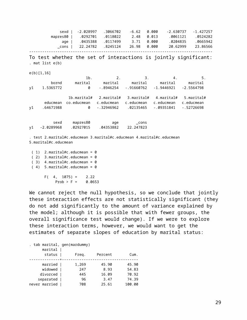
Others use cutoffs of 5 or even 10. In the example above, there are no problems with multicollinearity regardless of the cutoff we pick.
In addition, the following symptoms may indicate a multicollinearity problem: large changes in coefficients when adding or deleting variables non-significant coefficients for variables that you know are theoretically important coefficients with signs opposite of those you expected based on theory or previous results large standard errors in comparison to the coefficient size two (or more) large coefficients with opposite signs, possibly non-significant all or most coefficients are not significant even though the F-test indicates the entire
regression model is significant
Solutions for multicollinearity problems:
1. See if you could create a meaningful scale from the variables that are highly correlated, and use that scale instead of the individual variables (i.e. several variables are reconceptualized as indicators of one underlying construct). . sum mapres80 papres80 Variable | Obs Mean Std. Dev. Min Max-------------+-------------------------------------------------------- mapres80 | 1619 40.96912 13.63189 17 86 papres80 | 2165 43.47206 12.40479 17 86The variables have the same scales so we can add them: . gen prestige=mapres80+papres80(1519 missing values generated)
If the scales were different, we would first standardize each of them:
. egen papres80std = std(papres80)(600 missing values generated)
. egen mapres80std = std(mapres80)(1146 missing values generated)
. sum mapres80std papres80std Variable | Obs Mean Std. Dev. Min Max-------------+-------------------------------------------------------- mapres80std | 1619 4.12e-09 1 -1.758312 3.303348 papres80std | 2165 -8.26e-11 1 -2.134019 3.42835
. gen prestige2=mapres80std+papres80std(1519 missing values generated)
. pwcorr prestige prestige2
| prestige presti~2-------------+------------------ prestige | 1.0000 prestige2 | 0.9994 1.0000
We can now use prestige variable in subsequent OLS regressions. We might want to report a Chronbach’s alpha – it indicates the reliability of the scale. It varies between 0 and 1, with 1 being perfect. Typically, alphas above .7 are considered acceptable, although some argue that those above .5 are ok.
29
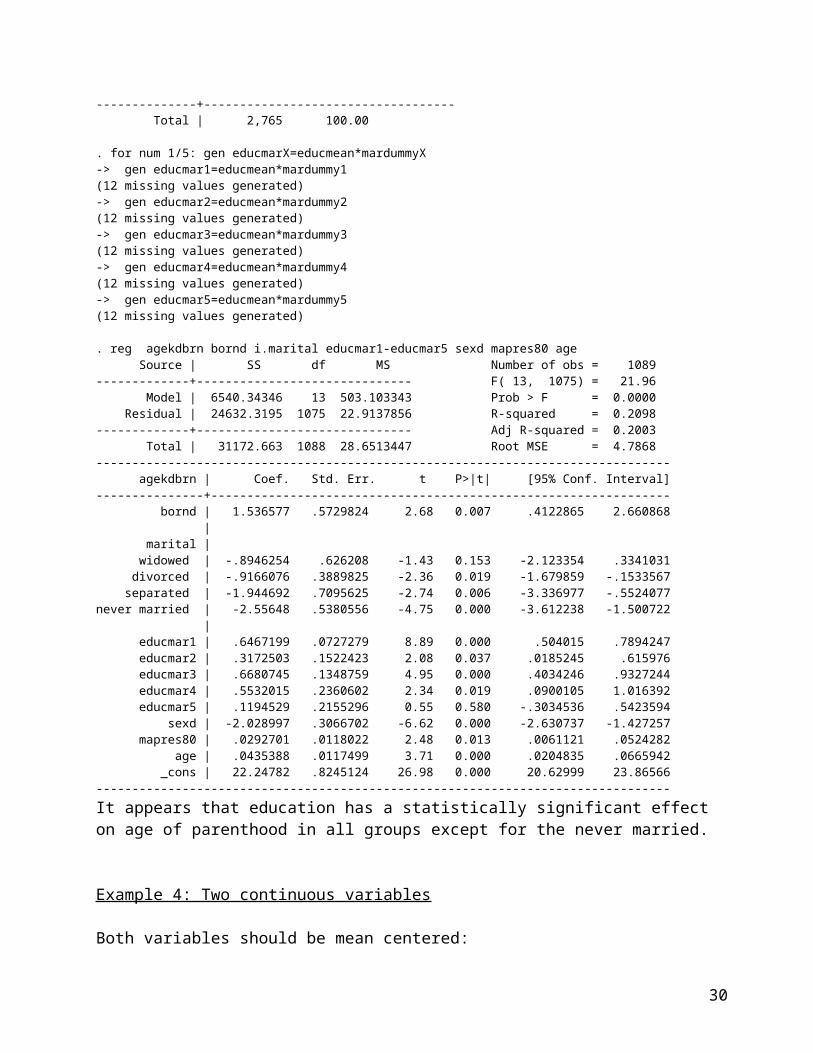
. alpha mapres80 papres80Test scale = mean(unstandardized items)Average interitem covariance: 56.39064Number of items in the scale: 2Scale reliability coefficient: 0.5036
2. Consider if all variables are necessary. Try to primarily use theoretical considerations -- automated procedures such as backward or forward stepwise regression methods (available via “sw regress” command) are potentially misleading; they capitalize on minor differences among regressors and do not result in an optimal set of regressors. If not too many variables, examine all possible subsets.
3. If using highly correlated variables is absolutely necessary for correct model specification, you can use biased estimates. The idea here is that we add a small amount of bias but increase the efficiency of the estimates for those highly correlated variables. The most common method of this type is ridge regression (see http://members.iquest.net/~softrx/ for the Stata module).
6. Heteroscedasticity
The problem of heteroscedasticity commonly refers to non-constant error variance (that’s opposite of homoscedasticity). We can examine this graphically as well as using formal tests. First, let's see if error variance changes across fitted values of our dependent variable:
. qui reg agekdbrn educ born sex mapres80 age
. rvfplot
-10
010
20R
esid
uals
15 20 25 30Fitted values
Can examine the same using a formal test:. hettestBreusch-Pagan / Cook-Weisberg test for heteroskedasticity Ho: Constant variance Variables: fitted values of agekdbrn chi2(1) = 21.44 Prob > chi2 = 0.0000
Since p<.05, we reject the null hypothesis of constant variance - the errors are heteroscedastic. Both the graph and the test indicate that the error variance is nonconsant (note the megaphone pattern).
30
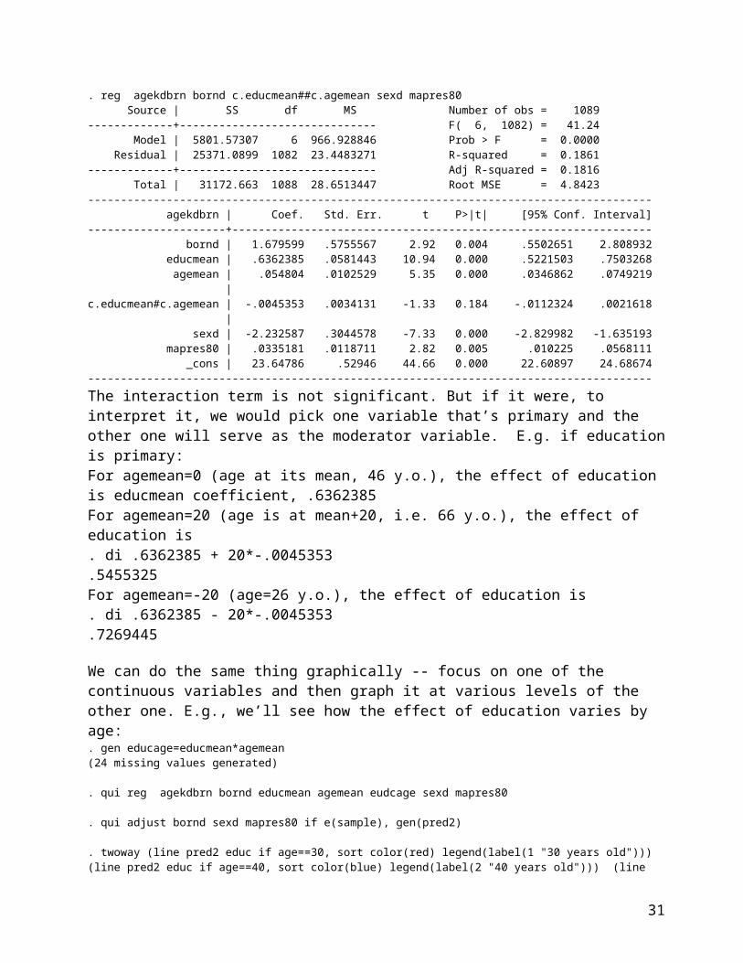
Now let's search if there is any systematic relationship between error variance and individual regressors. First, graphical examination:
. rvpplot educ
-10
010
20R
esid
uals
0 5 10 15 20highest year of school completed
.rvpplot age
-10
010
20R
esid
uals
20 40 60 80 100age of respondent
We can see the heteroscedasticity in both graphs, but it is much more severe for age. For a dummy variable, it is more difficult to examine it graphically:. rvpplot sex
-10
010
20R
esid
uals
1 1.2 1.4 1.6 1.8 2respondents sex
31
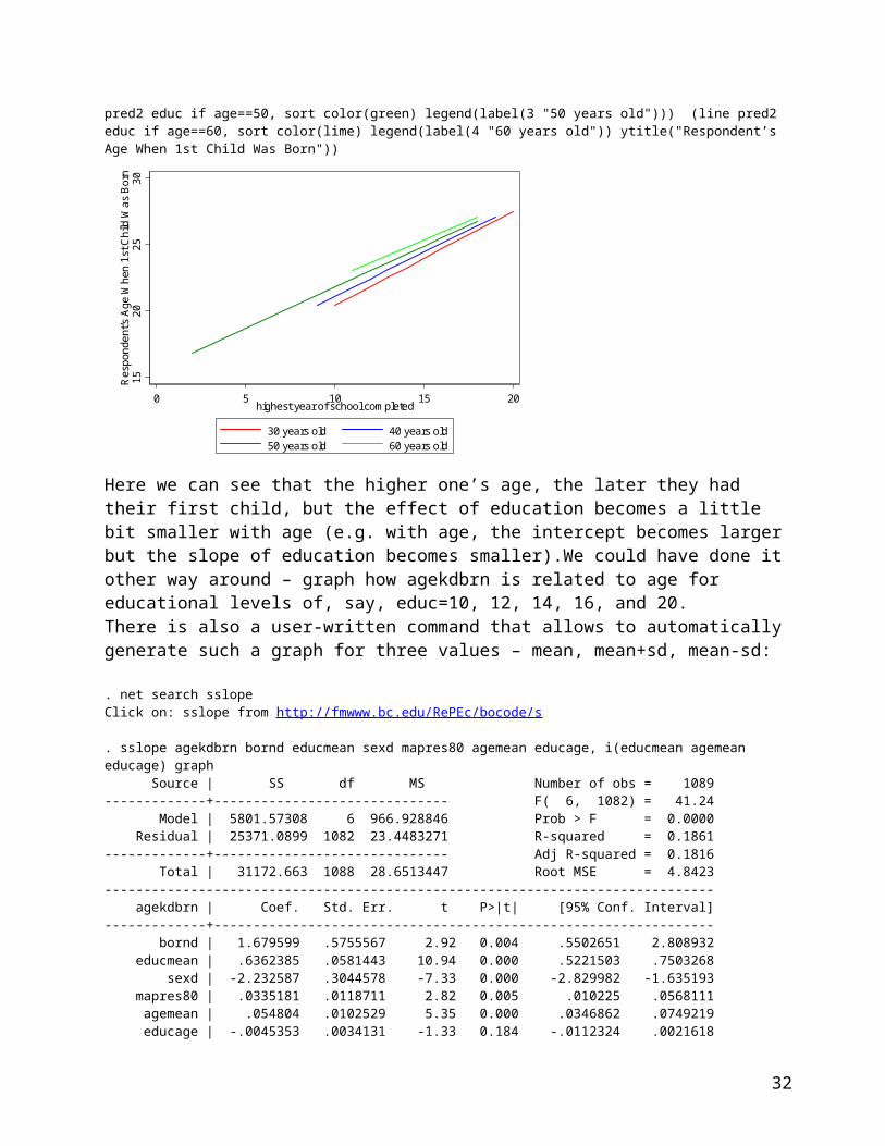
Now, let's use a formal test to examine the patterns of error variance across individual regressors:. hettest, rhs mtestBreusch-Pagan / Cook-Weisberg test for heteroskedasticity Ho: Constant variance--------------------------------------- Variable | chi2 df p -------------+------------------------- educ | 5.87 1 0.0154 # born | 0.00 1 0.9810 # sex | 9.19 1 0.0024 # mapres80 | 1.45 1 0.2279 # age | 10.26 1 0.0014 #-------------+-------------------------simultaneous | 25.78 5 0.0001--------------------------------------- # unadjusted p-values
It looks like a number of regressors are responsible for our problems.
Remedies:1. Transformations might help – it is especially important to consider the distribution of the dependent variable. As we discussed above, it is typically desirable, and can help avoid heteroscedasticity as well as non-normality problems, if the dependent variable is normally distributed. Let's examine whether the transformation we identified – reciprocal square root – would solve our heteroscedasticity problem.
. gen agekdbrnrr=1/(sqrt(agekdbrn))(810 missing values generated)
. reg agekdbrnrr educ born sex mapres80 age Source | SS df MS Number of obs = 1089-------------+------------------------------ F( 6, 1082) = 48.07 Model | .11381105 6 .018968508 Prob > F = 0.0000 Residual | .426934693 1082 .000394579 R-squared = 0.2105-------------+------------------------------ Adj R-squared = 0.2061 Total | .540745743 1088 .000497009 Root MSE = .01986------------------------------------------------------------------------------ agekdbrnrr | Coef. Std. Err. t P>|t| [95% Conf. Interval]-------------+---------------------------------------------------------------- educ | -.0024213 .0002353 -10.29 0.000 -.0028829 -.0019597 born | -.0070982 .0023638 -3.00 0.003 -.0117363 -.0024602 sex | .0095887 .0012506 7.67 0.000 .0071349 .0120425 mapres80 | -.0001494 .0000487 -3.07 0.002 -.000245 -.0000539 agemean | -.0003115 .0000434 -7.18 0.000 -.0003967 -.0002264 agemean2 | 8.86e-06 2.29e-06 3.87 0.000 4.37e-06 .0000134 _cons | .2373519 .0046505 51.04 0.000 .228227 .2464769------------------------------------------------------------------------------
. hettestBreusch-Pagan / Cook-Weisberg test for heteroskedasticity Ho: Constant variance Variables: fitted values of agekdbrnrr
chi2(1) = 0.35 Prob > chi2 = 0.5566. hettest, rhs mtest
Breusch-Pagan / Cook-Weisberg test for heteroskedasticity Ho: Constant variance
32
--------------------------------------- Variable | chi2 df p -------------+------------------------- educ | 0.63 1 0.4262 # born | 0.26 1 0.6111 # sex | 0.29 1 0.5932 # mapres80 | 0.73 1 0.3939 # age | 1.71 1 0.1911 #-------------+-------------------------simultaneous | 3.06 5 0.6900--------------------------------------- # unadjusted p-values
The heteroscedasticity problem has been solved. As I mentioned earlier, however, it is important to check that we did not introduce any nonlinearities by this transformation, and overall, transformations should be used sparsely - always consider ease of model interpretation as well. Also, sometimes when searching for a transformation to remedy heteroscedasticity, Box-Cox transformations can be very helpful, including the “transform both sides” (TBS) approach (see boxcox command).
2. Sometimes, dealing with outliers, influential observations, and nonlinearities might also help resolve heteroscedasticity problems. That is why I recommend testing with heteroscedasticity only after you’ve dealt with other problem.
3. Heteroscedasticity can also be a sign that some important factor is omitted, so you might want to rethink your model specification.
4. If nothing else works, we can obtain robust variance estimates using robust option in regress command (note that this is different from robust regression estimated by rreg!). These variance estimates do not rely on distributional assumptions and are therefore not sensitive to heteroscedasticity:
. reg agekdbrn educ born sex mapres80 age, robustLinear regression Number of obs = 1089 F( 5, 1083) = 47.74 Prob > F = 0.0000 R-squared = 0.1848 Root MSE = 4.8441------------------------------------------------------------------------------ | Robust agekdbrn | Coef. Std. Err. t P>|t| [95% Conf. Interval]-------------+---------------------------------------------------------------- educ | .6158833 .0640298 9.62 0.000 .4902467 .7415199 born | 1.679078 .5756992 2.92 0.004 .5494661 2.80869 sex | -2.217823 .3143631 -7.05 0.000 -2.834653 -1.600993 mapres80 | .0331945 .0122934 2.70 0.007 .009073 .0573161 age | .0582643 .0088246 6.60 0.000 .0409491 .0755795 _cons | 13.27142 1.239779 10.70 0.000 10.83877 15.70406------------------------------------------------------------------------------
33