Thesis Proposal

Complexity reduction in H.264/ AVC Motion Estimation using Compute Unified Device Architecture

Under guidance of

DR K R RAODEPARTMENT OF ELECTRICAL ENGINEERING

UNIVERSITY OF TEXAS AT ARLINGTON

Submitted by

TEJAS SATHE

tejas.sathe@mavs.uta.edu

List of acronyms

API: Application Programming Interface

AVC: Advanced Video Codec

CABAC: Context Based Adaptive Binary Arithmetic Coding

CPU: Central Processing Unit

CUDA: Compute Unified Device Architecture

GPGPU: General Purpose Computing on GPU

FLOPs: Floating Point Operations per second

JPEG: Joint Photographic Experts Group

MPEG: Moving Picture Experts Group

OpenMP: Open Multicore Programming

RDO: Rate Distortion Optimization

SIMD: Single Instruction Multiple Data

VLSI: Very Large Scale Integration

Objective

To reduce the motion estimation time in H.264 encoder by incorporating GPGPU technique using CUDA programming.

Introduction

Efficient digital representation of image and video signals has been the subject of

research over the last couple of decades. Growing availability of digital transmission links,

research in signal processing, VLSI technology and image compression, visual communications

and digital video coding technology are becoming more and more feasible, dramatically. A

diversity of products has been developed targeted for a wide range of emerging applications,

such as video on demand, digital TV/HDTV broadcasting, and multimedia image/video database

services.

The rapid growth of digital video coding technology has resulted in increased

commercial interest in video communications thereby arising need for international image and

video coding standards. The basis of large markets for video communication equipment and

digital video broadcasting is standardization of video coding algorithms.

MPEG-4 Part 10 or AVC (Advanced Video Coding) [5] –also called as H.264 is a

standard for video compression, and is currently one of the most commonly used formats for the

recording, compression, and distribution of high definition video. Without compromising the

image quality, an H.264 encoder can reduce the size of a digital video file by more than 80%

compared with the Motion JPEG format and as much as 50% more than with the MPEG-4 Part 2

standard. This implies much less network bandwidth and storage space are required for a video

file. Seen another way, much higher video quality can be achieved for a given bit rate.

Various electronic gadgets such as mobile phones and digital video players have adopted

H.264 [2], [5]. Service providers such as online video storage and telecommunications

companies are also beginning to adopt H.264. The standard has accelerated the adoption of

megapixel cameras since the highly efficient compression technology can reduce the large file

sizes and bit rates generated without compromising image quality.

H.264 Profiles [2]

The joint group involved in defining H.264 focused on creating a simple and clean

solution, limiting options and features to a minimum. An important aspect of the standard, as

with other video standards, is providing the capabilities in various profiles. Following sets of

capabilities are defined in H.264/AVC standard. These capabilities are referred to as

profiles (Fig.1). They target specific classes of applications.

Baseline Profile

1. Flexible macroblock order: macroblocks may not necessarily be in the raster scan

order. The map assigns macroblocks to a slice group.

2. Arbitrary slice order: the macroblock address of the first macroblock of a slice of a

picture may be smaller than the macroblock address of the first macroblock of some

other preceding slice of the same coded picture.

3. Redundant slice: this slice belongs to the redundant coded data obtained by same or

different coding rate, in comparison with previous coded data of same slice.

Main Profile

1. B slice (Bi-directionally predictive-coded slice): the coded slice by using inter-

prediction from previously decoded reference pictures, using at most two motion

vectors and reference indices to predict the sample values of each block.

2. Weighted prediction: scaling operation by applying a weighting factor to the samples

of motion-compensated prediction data in P or B slice.

3. CABAC (Context-based Adaptive Binary Arithmetic Coding) for entropy coding.

Extended Profile1. Includes all parts of Baseline Profile: flexible macroblock order, arbitrary slice order,

redundant slice2. SP slice: the specially coded slice for efficient switching between video streams,

similar to coding of a P slice.3. SI slice: the switched slice, similar to coding of an I slice.4. Data partition: the coded data is placed in separate data partitions, each partition can

be placed in different layer unit.5. B slice6. Weighted prediction

High Profiles

1. Includes all parts of Main Profile: B slice, weighted prediction, CABAC

2. Adaptive transform block size: 4x4 or 8x8 integer transform for luma samples

3. Quantization scaling matrices: different scaling according to specific frequency

associated with the transform coefficients in the quantization process to optimize the

subjective quality

Aiming at implementation of H.264 video encoder on handheld devices, in this thesis,

baseline profile is used.

Fig. 1 H.264 Profiles [9]

Encoder [2], [7]:

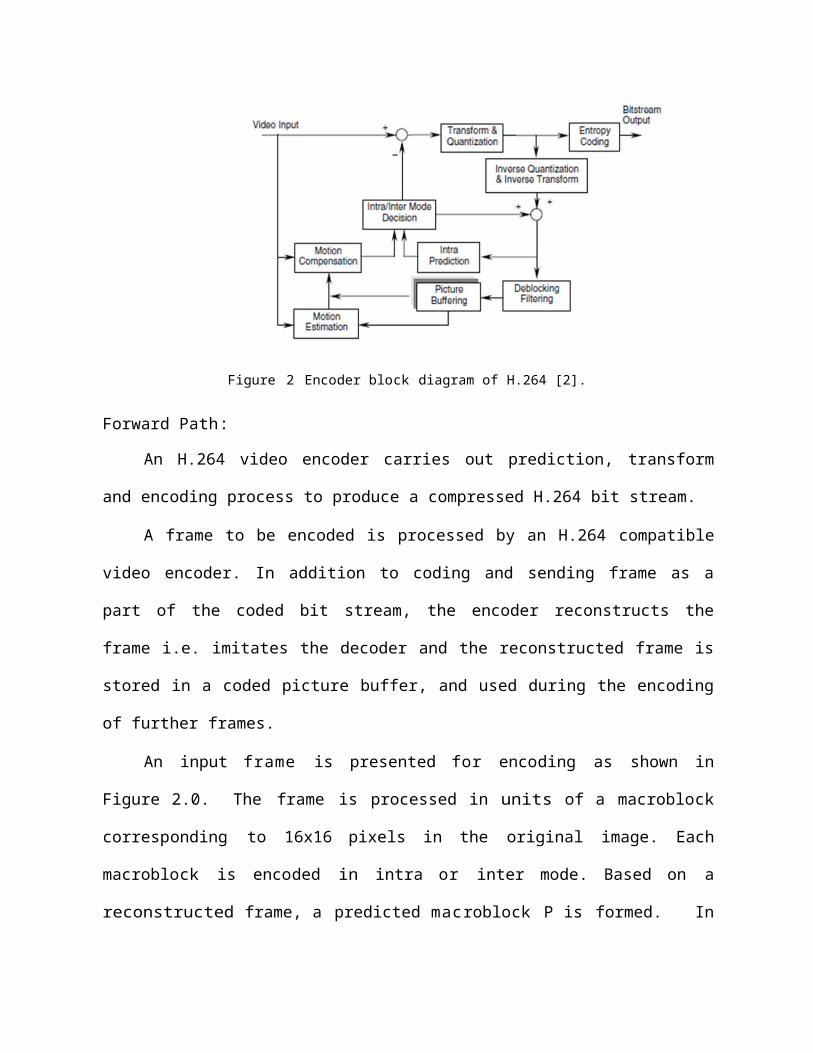
The encoder block diagram of H.264 is as shown in fig. 2

The encoder blocks can be divided into two categories:

1. Forward path

2. Reconstruction path

Figure 2 Encoder block diagram of H.264 [2].

Forward Path:

An H.264 video encoder carries out prediction, transform and encoding process to

produce a compressed H.264 bit stream.

A frame to be encoded is processed by an H.264 compatible video encoder. In addition

to coding and sending frame as a part of the coded bit stream, the encoder reconstructs the

frame i.e. imitates the decoder and the reconstructed frame is stored in a coded picture buffer,

and used during the encoding of further frames.

An input frame is presented for encoding as shown in Figure 2.0. The frame is

processed in units of a macroblock corresponding to 16x16 pixels in the original image.

Each macroblock is encoded in intra or inter mode. Based on a reconstructed frame, a

predicted macroblock P is formed. In intra mode , P is formed from samples in the

current frame that have been previously encoded, decoded and reconstructed. The

unfiltered samples are used to form P. In inter mode, P is formed by inter or motion-

compensated prediction from one or more reference frame(s). The prediction for each

macroblock may be formed from one or more past or future frames (in time order) that have

already been encoded and reconstructed.

In the encoder, the prediction macroblock P is subtracted from the current

macroblock. This produces a residual or difference macroblock. Using a block transform,

the difference macroblock is transformed and quantized to give a set of quantized transform

coefficients. These coefficients are rearranged and encoded using entropy encoder. The

entropy encoded coefficients, and the other information such as the macroblock prediction

mode, quantizer step size, motion vector information etc. required to decode the macroblock

form the compressed bitstream. This is passed to network abstraction layer (NAL) for

transmission or storage.

Reconstruction path:

In the reconstruction path, quantized macroblock coefficients are dequantized and are

re-scaled and inverse transformed to produce a difference macroblock. This is not identical

to the original difference macroblock, since quantization is a lossy process. The predicted

macroblock P is added to the difference macroblock to create a reconstructed macroblock,

a distorted version of the original macroblock. To reduce the effects of blocking distortion, a

de-blocking filter is applied and from a series of macroblocks, reconstructed reference

frame is created.

Decoder:

The decoder block diagram of H.264 is as shown in fig. 3

Figure 3 Decoder block diagram of H.264 [2].

The decoder carries out the complementary process of decoding, inverse transform and

reconstruction to produce a decoded video sequence.

The decoder receives a compressed bitstream from the NAL. The data elements are

entropy decoded and rearranged to produce a set of quantized coefficients. These are

rescaled and inverse transformed to give a difference macroblock. Using the other

information such as the macroblock prediction mode, quantizer step size, motion vector

information etc. decoded from the bit stream, the decoder creates a prediction macroblock

P, identical to the original prediction P formed in the encoder. P is added to the

difference macroblock and this result is given to the deblocking filter to create the

decoded macroblock.

The reconstruction path in the encoder ensures that both encoder and decoder use

identical reference frames to create the prediction P. If this is not the case, then the

predictions P in encoder and decoder will not be identical, leading to an increasing error or

drift between the encoder and decoder.

Intra Prediction [2], [10], [11]:

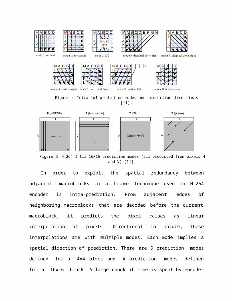
Adaptive intra directional prediction modes for (4x4) and (16x16) blocks are shown in Fig. 4 and Fig. 5

Figure 4 Intra 4x4 prediction modes and prediction directions [11].

Figure 5 H.264 Intra 16x16 prediction modes (all predicted from pixels H and V) [11].

In order to exploit the spatial redundancy between adjacent macroblocks in a frame

technique used in H.264 encoder is intra-prediction. From adjacent edges of neighboring

macroblocks that are decoded before the current macroblock, it predicts the pixel values as

linear interpolation of pixels. Directional in nature, these interpolations are with multiple

modes. Each mode implies a spatial direction of prediction. There are 9 prediction modes

defined for a 4x4 block and 4 prediction modes defined for a 16x16 block. A large

chunk of time is spent by encoder in the union of all mode evaluations, cost comparisons and

exhaustive search inside motion estimation (ME). In fact, complex and exhaustive ME

evaluation is the key to good performance achieved by H.264, but the cost is in the

encoding time.

Inter Prediction [2], [8], [10]:

There exists a lot of redundancy between successive frames, called as temporal

redundancy. The technique used in H.264 encoder to exploit the temporal redundancy is called

inter prediction. It includes motion estimation (ME) and motion compensation (MC). The

ME/ MC process performs prediction. It generates a predicted version of a macroblock, by

choosing another similarly sized rectangular array of pixels from a previously decoded

reference picture and translating the reference array to the position of the current

rectangular array. The translation from other positions of the array in the reference picture

is specified with quarter p i x e l precision.

Figure 6 Multi-frame bidirectional motion compensation in H.264 [14]

H.264/AVC supports multi-picture motion-compensated prediction [14]. That is, more

than one prior-coded picture can be used as a reference for motion-compensated prediction.

Up to 16 frames can be used as reference frames. In addition to the motion vector, the

picture reference parameters are also transmitted. Both the encoder and decoder have to

store the reference pictures used for Inter- picture prediction in a multi-picture buffer.

The decoder replicates the multi-picture buffer of the encoder, according to the reference

picture buffering type and any memory management control operations that are specified

in the bit stream. B frames use both a past and future frame as a reference. This

technique is called bidirectional prediction (Fig. 6). B frames provide most compression and

also reduce the effect of noise by averaging two frames. B frames are not used in the

baseline profile.

Figure 7 Block sizes used for motion compensation [5].

H.264 supports motion compensation block sizes ranging from 16x16 to 16x8,

8x16, 8x8, 8x4, 4x8 and 4x4 sizes as shown in Figure 7. This method of partitioning

macroblocks into motion compensated sub-blocks of varying sizes is known as tree

structured motion compensation.

Higher coding efficiency in H.264 is accomplished by a number of advanced features

incorporated in the standard. One of the new features is multi-mode selection for intra-frames

and inter-frames. Spatial redundancy in I-frames can be dramatically reduced by Intra-frame

mode selection while inter-frame mode selection significantly affects the output quality of P-/B-

frames by selecting an optimal block size with motion vectors or a mode for each macroblock.

In H.264, the coding block size is not fixed. It supports variable block sizes to minimize the

overall error.

In H.264 standard, rate distortion optimization (RDO) [14] technique is used to select the

best coding mode among all the possible modes [2]. RDO helps maximize image quality and

minimize coding bits by checking all the mode combinations for each MB exhaustively.

However, the RDO technique increases the coding complexity drastically, which makes H.264

not suitable for real-time applications.

Now a days, personal computers and video game consoles are consumer electronics

devices commonly equipped with GPUs. Recently, the progress of GPUs has caught a lot of

attention; they have changed from fixed pipelines to programmable pipelines [17]. The hardware

design of GPU also includes multiple cores, bigger memory sizes and better interconnection

networks which offer practical and acceptable solutions for speeding both graphics and non-

graphics applications. Highly parallel, GPUs are used as a coprocessor to assist the Central

Processing Unit (CPU) in computing massive data. NVIDIA developed a powerful GPU

architecture denominated Compute Unified Device Architecture (CUDA) [17], which is formed

by a single program multiple data computing device. Thus, the motion estimation algorithm

developed in the H.264/AVC encoding algorithm fits well in the GPU philosophy and offers a

new challenge for the GPUs.

Driven by the high demand for real time, high-definition 3D graphics, the programmable

Graphic Processor Unit or GPU has evolved into a highly parallel, multithreaded, many core

processor with tremendous computational horsepower and very high memory bandwidth. GPU,

which typically handles computation only for computer graphics, can be used to perform

computation in applications traditionally handled by the CPU. This technique is known as

General Purpose Computing on GPU (GPGPU). It is proposed that GPU can be used as a

general purpose computing unit for motion estimation in H.264/AVC.

The reason behind the discrepancy in floating-point capability between the CPU and the

GPU is that the GPU is specialized for compute-intensive, highly parallel computation – exactly

what graphics rendering is about – and therefore designed such that more transistors are devoted

to data processing rather than data caching and flow control.

Features of a GPU:

1. Data parallel algorithms leverage GPU attributes

2. Fine-grain SIMD parallelism

3. Low-latency floating point (FP) computation

4. Game effects (FX) physics, image processing

5. Computational engineering, matrix algebra, convolution, correlation.

Comparison between CPUs and GPUs:

3.0 GHz dual-core Pentium4: 24.6 GFLOPs

NVIDIA GeForceFX 7800: 165 GFLOPs

1066 MHz FSB Pentium Extreme Edition : 8.5 GB/s

ATI Radeon X850 XT Platinum Edition: 37.8 GB/s

CPUs: 1.4× annual growth

GPUs: 1.7×(pixels) to 2.3× (vertices) annual growth

The multicore revolution and the ever-increasing complexity of computing systems is

dramatically changing system design, analysis and programming of computing platforms [17].

Future architectures will feature hundreds to thousands of simple processors and on-chip

memories connected through a network-on-chip. Architectural simulators will remain primary

tools for design space exploration, software development and performance evaluation of these

massively parallel architectures. However, architectural simulation performance is a serious

concern, as virtual platforms and simulation technology are not able to tackle the complexity of

thousands of core future scenarios.

Many applications that process large data sets can use a data-parallel programming

model to speed up the computations [17]. In 3D rendering, large sets of pixels and vertices are

mapped to parallel threads. Similarly, image and media processing applications such as post-

processing of rendered images, video encoding and decoding, image scaling, stereo vision, and

pattern recognition can map image blocks and pixels to parallel processing threads. In fact,

many algorithms outside the field of image rendering and processing are accelerated by data-

parallel processing, from general signal processing or physics simulation to computational

finance or computational biology.

Due to the rapid growth of graphics processing unit (GPU) processing capability, using

GPU as a coprocessor to assist the central processing unit (CPU) in computing massive data

becomes essential. The CUDA enhances the programmability and flexibility for general-purpose

computation on GPU. Experimental results also show that, with the assistance of GPU, the

processing time is several times faster than that of using CPU only [16].

CUDA™: a General-Purpose Parallel Computing Architecture [17]

In November 2006, NVIDIA introduced CUDA™, a general purpose parallel computing

architecture – with a new parallel programming model and instruction set architecture.

The advent of multicore CPUs and many core GPUs means that mainstream processor

chips are now parallel systems. Furthermore, their parallelism continues to scale with Moore’s

law. The challenge is to develop application software that transparently scales its parallelism to

leverage the increasing number of processor cores, much as 3D graphics applications

transparently scale their parallelism to many core GPUs with widely varying numbers of cores.

The CUDA parallel programming model is designed to overcome this challenge while

maintaining a low learning curve for programmers familiar with standard programming

languages such as C. At its core are three key abstractions – a hierarchy of thread groups, shared

memories, and barrier synchronization – that are simply exposed to the programmer as a

minimal set of language extensions. These abstractions provide fine-grained data parallelism

and thread parallelism, nested within coarse-grained data parallelism and task parallelism. They

guide the programmer to partition the problem into coarse sub-problems that can be solved

independently in parallel by blocks of threads, and each sub-problem into finer pieces that can

be solved cooperatively in parallel by all threads within the block.

Each block of threads in a GPU can be scheduled on any of the available processor

cores, in any order, concurrently or sequentially, so that a compiled CUDA program can execute

on any number of processor cores and only the runtime system needs to know the physical

processor count.

This scalable programming model allows the CUDA architecture to span a wide market

range by simply scaling the number of processors and memory partitions: from the high-

performance enthusiast GeForce GPUs and professional Quadro and Tesla computing products

to a variety of inexpensive, mainstream GeForce GPUs. A multithreaded program is partitioned

into blocks of threads that execute independently from each other, so that a GPU with more

cores will automatically execute the program in less time than a GPU with fewer cores. Figures

8 and 9 show grid of thread blocks and hardware model.

Figure 8 Grid of thread blocks [17]

Figure 9 Hardware model [17]

Proposal

In this thesis, it is proposed that using CUDA, H.264 encoder motion estimation time complexity can be reduced to great extent.

References

1. ITU-T Rec. H.264 | ISO/IEC 14496-10: Information Technology – Coding of Audio-visual Objects, Part 10: Advanced Video Coding 2002.

2. T.Wiegand, et al, “Overview of the H.264/AVC Video Coding Standard.” IEEE Trans. Circuits and Syst. for Video Technol., Vol. 13, pp. 560-576, July 2003.

3. Z.Chen, et al, “Fast Integer Pixel and Fractional Pixel Motion Estimation for JVT.” Doc. #JVT-F017, Dec. 2002.

4. B.Hsieh, et al, “Fast Motion Estimation for H.264/MPEG-4 AVC by Using Multiple Reference Frame Skipping Criteria.” VCIP 2003, Proceedings of SPIE, Vol. 5150, pp. 1551-1560, Oct. 2003.

5. A.Puri, et al, “Video coding using the H.264/MPEG-4 AVC compression standard”, Signal Processing: Image Communication, vol.19, pp. 793-849, Oct. 2004.

6. H.264/AVC JM software: http://iphome.hhi.de/suehring/tml/

7. An overview of the H.264 encoder: www.vcodex.com

8. J. Ren, et al, “Computationally efficient mode selection in H.264/AVC video coding”, IEEE Trans. on Consumer Electronics, vol. 54, pp. 877 – 886, May 2008.

9. I. Richardson, “The H.264 advanced video compression standard” –second edition, Wiley, 2010.

10. Soon-kak Kwon, et al “Overview of H.264/MPEG-4 part 10”, J. VCIR, vol.17, pp. 186-216, April 2006.

11. J. Kim, et al “Complexity Reduction Algorithm for Intra Mode Selection in H.264/AVC Video Coding”, ACIVS 2006, LNCS 4179, pp. 454 – 465, 2006. Springer-Verlag Berlin Heidelberg, 2006.

12. YUV test video sequences : http://trace.eas.asu.edu/yuv/

13. R. Rodriguez, et al, “Accelerating H.264 Inter Prediction in a GPU by using CUDA”, Consumer Electronics (ICCE), pp. 463 – 464, 2010.

14. Ling-Jiao Pan, et al, “Fast Mode Decision Algorithms for Inter/Intra Prediction in H.264 Video Coding”, PCM 2007, LNCS 4810, pp. 158–167, 2007. Springer-Verlag Berlin Heidelberg 2007.

15. Z. Wei, et al, “Implementation of H.264 on Mobile Device”, Consumer Electronics, IEEE Trans Vol. 53, pp. 1109 – 1116, Aug. 2007.

16. Wei-Nien Chen, et al, “H.264/AVC Motion Estimation Implementation On Compute Unified Device Architecture (CUDA)” Multimedia and Expo, 2008 IEEE International Conference, pp. 697 – 700, 2008.

17. CUDA reference manual: http://developer.nvidia.com/cuda-downloads