· Web viewMatrix Much like available commercial softwares, Cemmath adopts class 'matrix' as the most valueable data structure. For concise explanation, we employ mathematical expression

[100] 211 Matrix, FastRead-Tutorial by www.msharpmath.com

[100] 211 revised on 2012.12.03 cemmath

The Simple is the Best

Matrix

Much like available commercial softwares, Cemmath adopts class 'matrix' as the most valueable data structure. For concise explanation, we employ mathematical expression for a matrix A of dimension m×n

A=(aij )=[ a11 a12 … a1n

a21 a22 ⋯ a2n

⋮ ⋮ ⋱ ⋮am1 am2 ⋯ amn

]Most operations on matrices will be described by representative element ( aij ). We presume that readers are familiar with matrix operations from mathematics.

// basic matrices// assignment by a matrix and scalar // reading/writing matrices to file// subscripts (read and write)// unary operation (read-only)// binary operations ( double or complex s, matrix A, B )// compound assignment ( double or complex s, matrix A, B )// one-dimensional treatment ( matrix A, B )// conditional operations// relational operations ( matrix A, double x, complex z )// special binary operations (int n, double or complex s, matrix A, B )// priorities of operations for matrices// index manipulating (read-only)// rows, columns and diagonals (read and write)// submatrix (read and write)// deleting elements

1


// extending matrices// superposition of operations// 'figure'-returning functions// piecewise polynomials// 'poly'-returning functions// 'matrix'-returning functions// column-first operations// 'double'-returning functions// 'tuple'-returning functions// matrix argument functions// useful dot functions for matrices// special matrices// matrix array// matrix declaration// tensor-related functions for stress analysis// geometry-returning functions// application to triangle solution

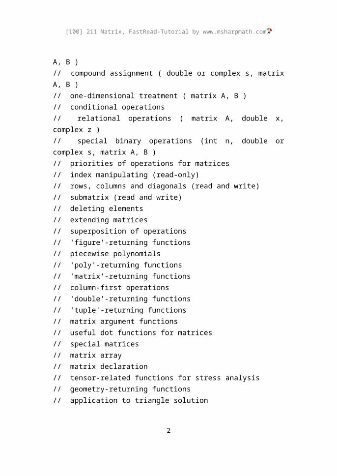
//----------------------------------------------------------------------// Basic Matrices//----------------------------------------------------------------------

// 0 x 0 matrix (can be used to declare matrix variables) []

// list of numbers or matrix inside a pair of [][ a_11, ... , a_1n; a_21, ... a_2n; ... ; a_n1,..., a_nn ]

a : b // [ a, a+1,… ] if a < b, otherwise [a,a-1,…]a : h : b // the same as (a,b).step(h)

(a,b) .step(h) // [ a, a+h, a+2h, ... ](a,b) .span(n,g=1) // [ x_1 = a, x_2, …, x_n = b ], dx_i = g dx_(i-1)(a,h) .march(n,g=1) // [ a, a+h(1),... , a+h(1+g+...+g^(n-2)) ](a,b) .logspan(n,g=1) // 10.^( (log10(a),log10(b)).span(n,g=1) )

.e_k(n) // k-th unit vector in the n-dimensional space

.I(m,n=m) // if i = j, a_ij = 1. Otherwise a_ij = 0eye(m,n=m) // .I(m,n=m) ones(m,n=m) // all-ones matrix

2


zeros(m,n=m) // all-zeros matrix.I(A) eye(A) // .I(A.m,A.n), same size with Aones(A) // ones(A.m,A.n), same size with Azeros(A) // zeros(A.m,A.n), same size with A

// 0 x 0 matrix can be used to declare a variable as a matrix#> A = []; A = []

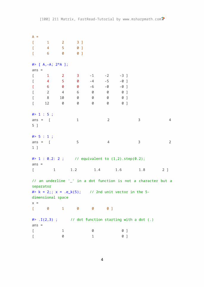
// separate rows by a semi-colon ';' and elements by a comma ','#> A = [ 1,2,3; 4,5; 6 ]; // A is changed from 0 x 0 to 3 x 3 matrixA =[ 1 2 3 ][ 4 5 0 ][ 6 0 0 ]

#> [ A,-A; 2*A ];ans =[ 1 2 3 -1 -2 -3 ][ 4 5 0 -4 -5 -0 ][ 6 0 0 -6 -0 -0 ][ 2 4 6 0 0 0 ][ 8 10 0 0 0 0 ][ 12 0 0 0 0 0 ]

#> 1 : 5 ;ans = [ 1 2 3 4 5 ]

#> 5 : 1 ;ans = [ 5 4 3 2 1 ]

#> 1 : 0.2: 2 ; // equivalent to (1,2).step(0.2);ans =[ 1 1.2 1.4 1.6 1.8 2 ]

// an underline '_' in a dot function is not a character but a separator#> k = 2;; x = .e_k(5); // 2nd unit vector in the 5-dimensional spacex =[ 0 1 0 0 0 ]

#> .I(2,3) ; // dot function starting with a dot (.)ans =[ 1 0 0 ][ 0 1 0 ]

3


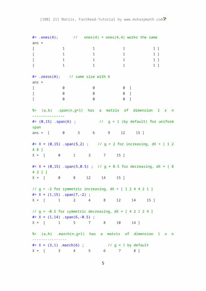
#> .ones(4); // ones(4) = ones(4,4) works the sameans =[ 1 1 1 1 ][ 1 1 1 1 ][ 1 1 1 1 ][ 1 1 1 1 ]

#> .zeros(A); // same size with Aans =[ 0 0 0 ][ 0 0 0 ][ 0 0 0 ]

%> (a,b) .span(n,g=1) has a matrix of dimension 1 x n ---------------#> (0,15) .span(6) ; // g = 1 (by default) for uniform spanans = [ 0 3 6 9 12 15 ]

#> X = (0,15) .span(5,2) ; // g = 2 for increasing, dX = [ 1 2 4 8 ]X = [ 0 1 3 7 15 ]

#> X = (0,15) .span(5,0.5) ; // g = 0.5 for decreasing, dX = [ 8 4 2 1 ]X = [ 0 8 12 14 15 ]

// g = -2 for symmetric increasing, dX = [ 1 2 4 4 2 1 ]#> X = (1,15) .span(7,-2) ; X = [ 1 2 4 8 12 14 15 ]

// g = -0.5 for symmetric decreasing, dX = [ 4 2 1 2 4 ]#> X = (1,14) .span(6,-0.5) ; X = [ 1 5 7 8 10 14 ]

%> (a,h) .march(n,g=1) has a matrix of dimension 1 x n ----------------#> X = (3,1) .march(6) ; // g = 1 by defaultX = [ 3 4 5 6 7 8 ]

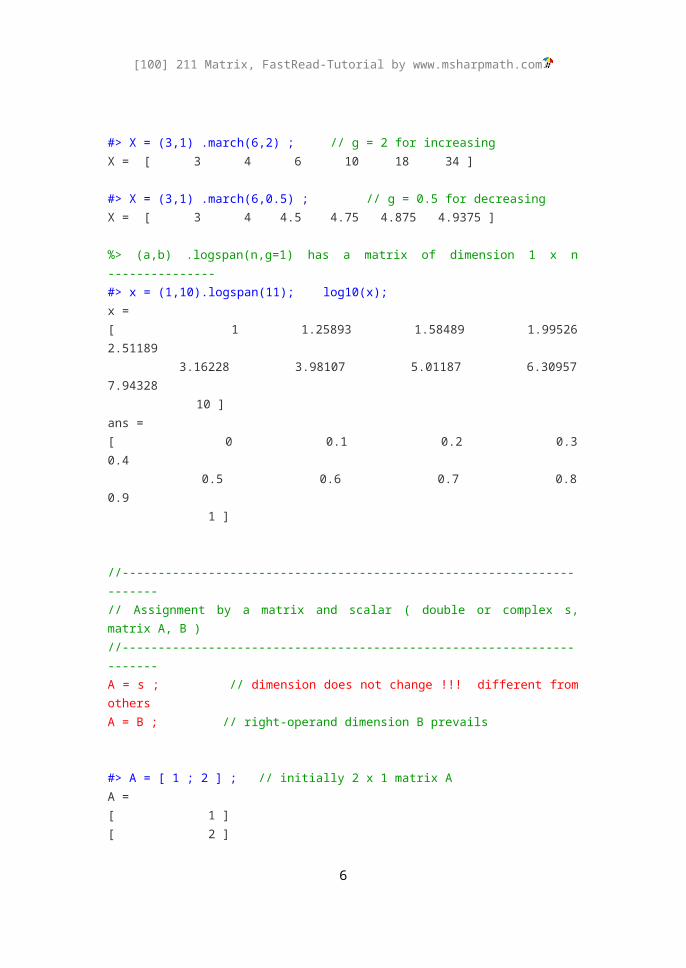
#> X = (3,1) .march(6,2) ; // g = 2 for increasingX = [ 3 4 6 10 18 34 ]

#> X = (3,1) .march(6,0.5) ; // g = 0.5 for decreasingX = [ 3 4 4.5 4.75 4.875 4.9375 ]

%> (a,b) .logspan(n,g=1) has a matrix of dimension 1 x n ---------------#> x = (1,10).logspan(11); log10(x);x =[ 1 1.25893 1.58489 1.99526 2.51189 3.16228 3.98107 5.01187 6.30957 7.94328

4


10 ]ans =[ 0 0.1 0.2 0.3 0.4

0.5 0.6 0.7 0.8 0.9 1 ]

//----------------------------------------------------------------------// Assignment by a matrix and scalar ( double or complex s, matrix A, B )//----------------------------------------------------------------------A = s ; // dimension does not change !!! different from othersA = B ; // right-operand dimension B prevails

#> A = [ 1 ; 2 ] ; // initially 2 x 1 matrix AA =[ 1 ][ 2 ]

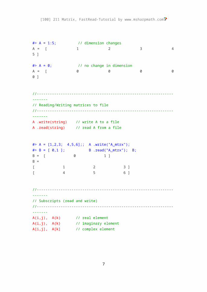
#> A = 1:5; // dimension changesA = [ 1 2 3 4 5 ]

#> A = 0; // no change in dimensionA = [ 0 0 0 0 0 ]

//----------------------------------------------------------------------// Reading/Writing matrices to file//----------------------------------------------------------------------A .write(string) // write A to a fileA .read(string) // read A from a file

#> A = [1,2,3; 4,5,6];; A .write("A_mtrx");#> B = [ 0,1 ]; B .read("A_mtrx"); B;B = [ 0 1 ]B =[ 1 2 3 ][ 4 5 6 ]

//----------------------------------------------------------------------// Subscripts (read and write)//----------------------------------------------------------------------A(i,j), A(k) // real element

5


A{i,j}, A{k} // imaginary elementA[i,j], A[k] // complex element

A=(aij )=[ a11 a12 … a1n

a21 a22 ⋯ a2n

⋮ ⋮ ⋱ ⋮am1 am2 ⋯ amn

]one-dimensional index k=i+m( j−1)

A=(ak)=[a1 am+1 … a( n−1)m+1

a2 am+2 ⋯ a( n−1)m+2

⋮ ⋮ ⋱ ⋮am a2m ⋯ amn

] , k=i+m( j−1)

These two notations can be converted by

k = A.k(i,j) // in matlab, k = sub2ind( size(A), i,j )(i,j) = A.ij(k) ; // in matlab, [i,j] = ind2sub( size(A), k )i = A.i(k) // i-th row for k-th linear indexj = A.j(k) // j-th column for k-th linear index

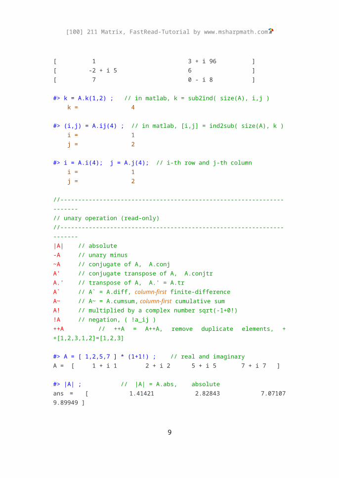
#> A = [ 1, 3-4! ; -2+5!, 6; 7, -8i ];A =[ 1 3 - i 4 ][ -2 + i 5 6 ][ 7 0 - i 8 ]

#> A(2,1); A{2,1}; A[2,1]; // access to -2+5!ans = -2ans = 5ans = -2 + 5!

#> A{4} += 100; A ; // imaginary element changedans = 96A =[ 1 3 + i 96 ][ -2 + i 5 6 ][ 7 0 - i 8 ]

#> k = A.k(1,2) ; // in matlab, k = sub2ind( size(A), i,j )

6


k = 4

#> (i,j) = A.ij(4) ; // in matlab, [i,j] = ind2sub( size(A), k ) i = 1 j = 2

#> i = A.i(4); j = A.j(4); // i-th row and j-th column i = 1 j = 2

//----------------------------------------------------------------------// unary operation (read-only)//----------------------------------------------------------------------|A| // absolute-A // unary minus~A // conjugate of A, A.conjA' // conjugate transpose of A, A.conjtrA.' // transpose of A, A.' = A.trA` // A` = A.diff, column-first finite-differenceA~ // A~ = A.cumsum, column-first cumulative sumA! // multiplied by a complex number sqrt(-1+0!)!A // negation, ( !a_ij )++A // ++A = A++A, remove duplicate elements, ++[1,2,3,1,2]=[1,2,3]

#> A = [ 1,2,5,7 ] * (1+1!) ; // real and imaginaryA = [ 1 + i 1 2 + i 2 5 + i 5 7 + i 7 ]

#> |A| ; // |A| = A.abs, absoluteans = [ 1.41421 2.82843 7.07107 9.89949 ]

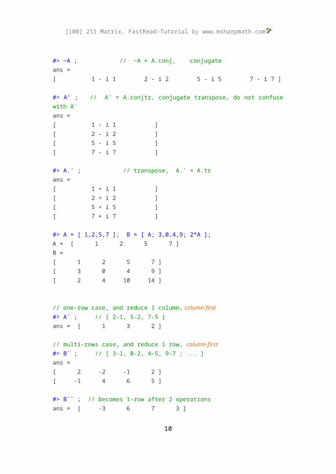
#> ~A ; // ~A = A.conj, conjugateans =[ 1 - i 1 2 - i 2 5 - i 5 7 - i 7 ]

#> A' ; // A' = A.conjtr, conjugate transpose, do not confuse with A`ans =[ 1 - i 1 ][ 2 - i 2 ][ 5 - i 5 ][ 7 - i 7 ]

#> A.' ; // transpose, A.' = A.trans =[ 1 + i 1 ][ 2 + i 2 ]

7


[ 5 + i 5 ][ 7 + i 7 ]

#> A = [ 1,2,5,7 ]; B = [ A; 3,0,4,9; 2*A ];A = [ 1 2 5 7 ]B =[ 1 2 5 7 ][ 3 0 4 9 ][ 2 4 10 14 ]

// one-row case, and reduce 1 column, column-first#> A` ; // [ 2-1, 5-2, 7-5 ]ans = [ 1 3 2 ]

// multi-rows case, and reduce 1 row, column-first#> B` ; // [ 3-1, 0-2, 4-5, 9-7 ; ... ]ans =[ 2 -2 -1 2 ][ -1 4 6 5 ]

#> B`` ; // becomes 1-row after 2 operationsans = [ -3 6 7 3 ]

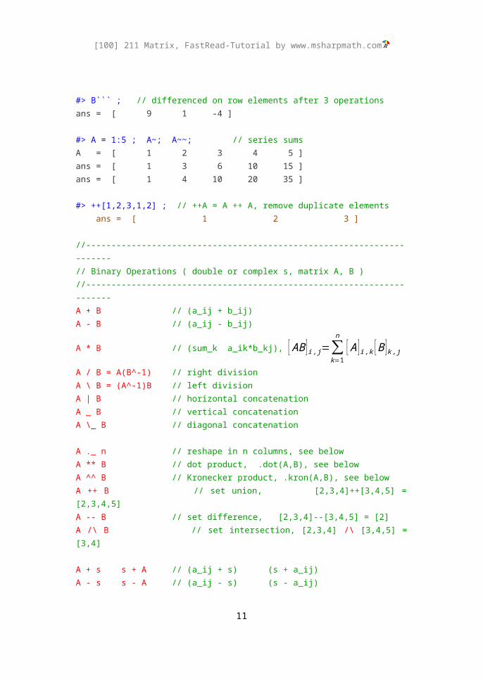
#> B``` ; // differenced on row elements after 3 operationsans = [ 9 1 -4 ]

#> A = 1:5 ; A~; A~~; // series sumsA = [ 1 2 3 4 5 ]ans = [ 1 3 6 10 15 ]ans = [ 1 4 10 20 35 ]

#> ++[1,2,3,1,2] ; // ++A = A ++ A, remove duplicate elements ans = [ 1 2 3 ]

//----------------------------------------------------------------------// Binary Operations ( double or complex s, matrix A, B )//----------------------------------------------------------------------A + B // (a_ij + b_ij)A - B // (a_ij - b_ij)

A * B // (sum_k a_ik*b_kj), [AB ]i , j=∑k=1

n

[A ]i , k [B ]k , jA / B = A(B^-1) // right divisionA \ B = (A^-1)B // left divisionA | B // horizontal concatenation

8


A _ B // vertical concatenationA \_ B // diagonal concatenation

A ._ n // reshape in n columns, see belowA ** B // dot product, .dot(A,B), see belowA ^^ B // Kronecker product, .kron(A,B), see belowA ++ B // set union, [2,3,4]++[3,4,5] = [2,3,4,5]A -- B // set difference, [2,3,4]--[3,4,5] = [2]A /\ B // set intersection, [2,3,4] /\ [3,4,5] = [3,4]

A + s s + A // (a_ij + s) (s + a_ij)A - s s - A // (a_ij - s) (s - a_ij)A * s s * A // (a_ij * s) (s * a_ij)A / s ... // (a_ij / s)... s \ A // (s \ a_ij)A ^ s ... // square matrix only

A .* B // (a_k * b_k), element-by-element operationsA ./ B // (a_k / b_k)A .\ B // (a_k \ b_k)A .^ B // (a_k ^ b_k)A .\ s // (a_k \ s)s ./ A // (s / a_k)A .^ s // (a_k ^ s)s .^ A // (s ^ a_k)

#> A = [ 1, 2, 3 ]; B = [ -4, 5, -6 ];A = [ 1 2 3 ]B = [ -4 5 -6 ]

#> A + B ;ans = [ -3 7 -3 ]

#> A - B ;ans = [ 5 -3 9 ]

#> A' * B ; // (3 x 1) * (1 x 3) = (3 x 3) dimensionans =[ -4 5 -6 ][ -8 10 -12 ][ -12 15 -18 ]

9


#> A * B' ; // (1 x 3) * (3 x 1) = (1 x 1) dimensionans = [ -12 ]

#> A * B ; // inner dimension mismatch90730: operator '*' : matrix inner dimension mismatch

#> A .* B ; // element-by-element multiplicationans = [ -4 10 -18 ]

#> A + 5 ; // constant is extended to m x n matrixans = [ 6 7 8 ]

#> 1 ./ A; // 1./A is an error, need space between 1 and dot(.)ans = [ 1 0.5 0.333333 ]

#> A = [ 1, 2, 3 ]; B = [ -4, 5 ]; A = [ 1 2 3 ] B = [ -4 5 ]

#> A | B ; // horizontal concatenation, .horzcat(A,B) ans = [ 1 2 3 -4 5 ]

#> A _ B ; // vertical concatenation, .vertcat(A,B) ans = [ 1 2 3 ] [ -4 5 0 ]

#> A \_ B ; // diagonal concatenation, .diagcat(A,B)ans = [ 1 2 3 0 0 ] [ 0 0 0 -4 5 ]

#> [ 1,2; 3,4 ] \_ [ 7-8i, 2; 5 ]; x = [ 1 2 0 0 ] [ 3 4 0 0 ] [ 0 0 7 - i 8 2 ] [ 0 0 5 0 ]

#> matrix.format("%3g");#> [2,3,4]++[3,4,5]; // A ++ B, set union ans = [ 2 3 4 5 ]

#> [2,3,4]--[3,4,5]; // A -- B, set difference ans = [ 2 ]

10


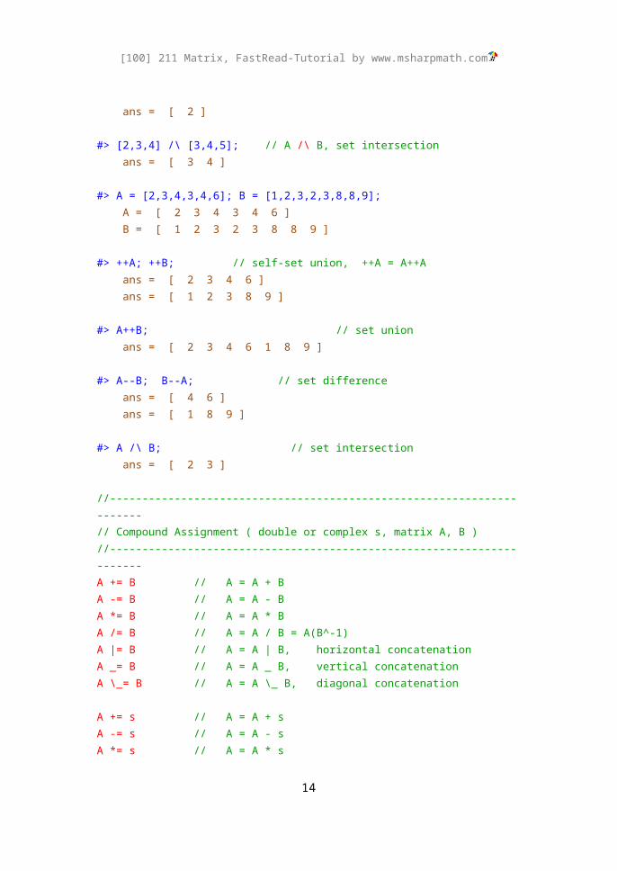
#> [2,3,4] /\ [3,4,5]; // A /\ B, set intersection ans = [ 3 4 ]

#> A = [2,3,4,3,4,6]; B = [1,2,3,2,3,8,8,9]; A = [ 2 3 4 3 4 6 ] B = [ 1 2 3 2 3 8 8 9 ]

#> ++A; ++B; // self-set union, ++A = A++A ans = [ 2 3 4 6 ] ans = [ 1 2 3 8 9 ]

#> A++B; // set union ans = [ 2 3 4 6 1 8 9 ]

#> A--B; B--A; // set difference ans = [ 4 6 ] ans = [ 1 8 9 ]

#> A /\ B; // set intersection ans = [ 2 3 ]

//----------------------------------------------------------------------// Compound Assignment ( double or complex s, matrix A, B )//----------------------------------------------------------------------A += B // A = A + BA -= B // A = A - BA *= B // A = A * BA /= B // A = A / B = A(B^-1)A |= B // A = A | B, horizontal concatenationA _= B // A = A _ B, vertical concatenationA \_= B // A = A \_ B, diagonal concatenation

A += s // A = A + sA -= s // A = A - sA *= s // A = A * sA /= s // A = A / sA ^= s // A = A ^ s

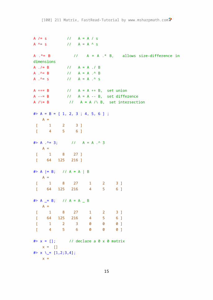
A .*= B // A = A .* B, allows size-difference in dimensionsA ./= B // A = A ./ BA .^= B // A = A .^ BA .^= s // A = A .^ s

A ++= B // A = A ++ B, set unionA --= B // A = A -- B, set differenceA /\= B // A = A /\ B, set intersection

11


#> A = B = [ 1, 2, 3 ; 4, 5, 6 ] ; A = [ 1 2 3 ] [ 4 5 6 ]

#> A .^= 3; // A = A .^ 3 A = [ 1 8 27 ] [ 64 125 216 ]

#> A |= B; // A = A | B A = [ 1 8 27 1 2 3 ] [ 64 125 216 4 5 6 ]

#> A _= B; // A = A _ B A = [ 1 8 27 1 2 3 ] [ 64 125 216 4 5 6 ] [ 1 2 3 0 0 0 ] [ 4 5 6 0 0 0 ]

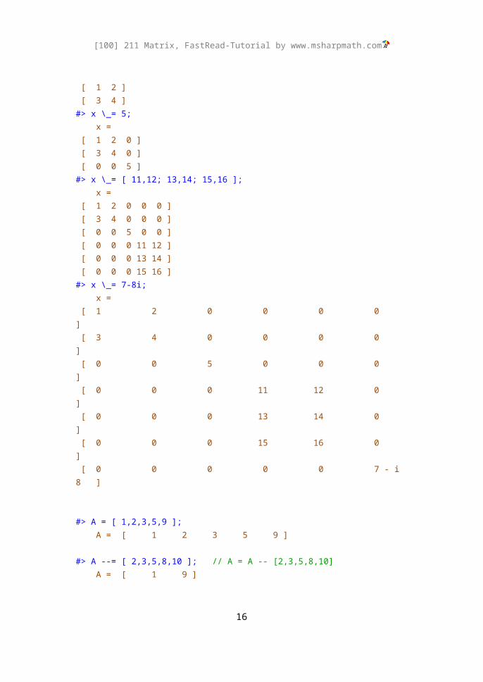
#> x = []; // declare a 0 x 0 matrix x = []#> x \_= [1,2;3,4]; x = [ 1 2 ] [ 3 4 ]#> x \_= 5; x = [ 1 2 0 ] [ 3 4 0 ] [ 0 0 5 ]#> x \_= [ 11,12; 13,14; 15,16 ]; x = [ 1 2 0 0 0 ] [ 3 4 0 0 0 ] [ 0 0 5 0 0 ] [ 0 0 0 11 12 ] [ 0 0 0 13 14 ] [ 0 0 0 15 16 ]#> x \_= 7-8i; x = [ 1 2 0 0 0 0 ] [ 3 4 0 0 0 0 ]

12


[ 0 0 5 0 0 0 ] [ 0 0 0 11 12 0 ] [ 0 0 0 13 14 0 ] [ 0 0 0 15 16 0 ] [ 0 0 0 0 0 7 - i 8 ]

#> A = [ 1,2,3,5,9 ]; A = [ 1 2 3 5 9 ]

#> A --= [ 2,3,5,8,10 ]; // A = A -- [2,3,5,8,10] A = [ 1 9 ]

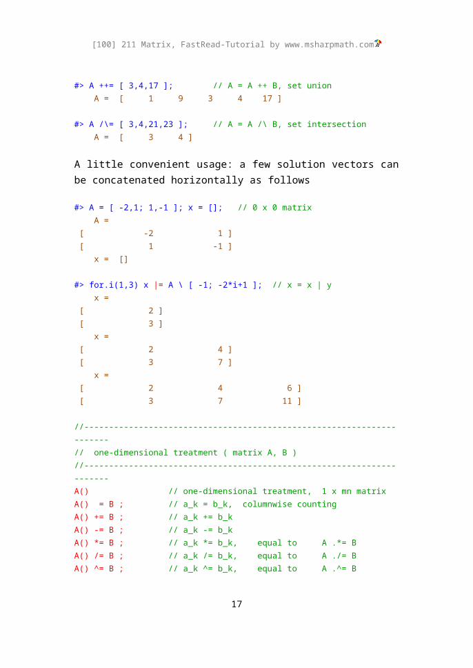
#> A ++= [ 3,4,17 ]; // A = A ++ B, set union A = [ 1 9 3 4 17 ]

#> A /\= [ 3,4,21,23 ]; // A = A /\ B, set intersection A = [ 3 4 ]

A little convenient usage: a few solution vectors can be concatenated horizontally as follows

#> A = [ -2,1; 1,-1 ]; x = []; // 0 x 0 matrix A = [ -2 1 ] [ 1 -1 ] x = []

#> for.i(1,3) x |= A \ [ -1; -2*i+1 ]; // x = x | y x = [ 2 ] [ 3 ] x = [ 2 4 ] [ 3 7 ] x = [ 2 4 6 ] [ 3 7 11 ]

//----------------------------------------------------------------------// one-dimensional treatment ( matrix A, B )//----------------------------------------------------------------------A() // one-dimensional treatment, 1 x mn matrixA() = B ; // a_k = b_k, columnwise countingA() += B ; // a_k += b_k

13


A() -= B ; // a_k -= b_kA() *= B ; // a_k *= b_k, equal to A .*= BA() /= B ; // a_k /= b_k, equal to A ./= BA() ^= B ; // a_k ^= b_k, equal to A .^= B

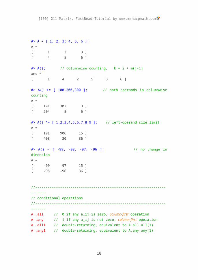
#> A = [ 1, 2, 3; 4, 5, 6 ];A =[ 1 2 3 ][ 4 5 6 ]

#> A(); // columnwise counting, k = i + m(j-1)ans =[ 1 4 2 5 3 6 ]

#> A() += [ 100,200,300 ]; // both operands in columnwise countingA =[ 101 302 3 ][ 204 5 6 ]

#> A() *= [ 1,2,3,4,5,6,7,8,9 ]; // left-operand size limitA =[ 101 906 15 ][ 408 20 36 ]

#> A() = [ -99, -98, -97, -96 ]; // no change in dimensionA =[ -99 -97 15 ][ -98 -96 36 ]

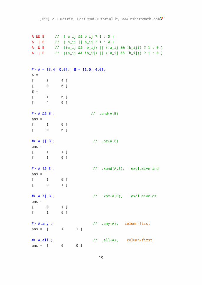
//----------------------------------------------------------------------// conditional operations//----------------------------------------------------------------------A .all // 0 if any a_ij is zero, column-first operationA .any // 1 if any a_ij is not zero, column-first operationA .all1 // double-returning, equivalent to A.all.all(1)A .any1 // double-returning, equivalent to A.any.any(1)

A && B // ( a_ij && b_ij ? 1 : 0 )A || B // ( a_ij || b_ij ? 1 : 0 )A !& B // ((a_ij && b_ij) || (!a_ij && !b_ij)) ? 1 : 0 )A !| B // ((a_ij && !b_ij) || (!a_ij && b_ij)) ? 1 : 0 )

14


#> A = [3,4; 0,0]; B = [1,0; 4,0];A =[ 3 4 ][ 0 0 ]B =[ 1 0 ][ 4 0 ]

#> A && B ; // .and(A,B)ans =[ 1 0 ][ 0 0 ]

#> A || B ; // .or(A,B)ans =[ 1 1 ][ 1 0 ]

#> A !& B ; // .xand(A,B), exclusive andans =[ 1 0 ][ 0 1 ]

#> A !| B ; // .xor(A,B), exclusive orans =[ 0 1 ][ 1 0 ]

#> A.any ; // .any(A), column-firstans = [ 1 1 ]

#> A.all ; // .all(A), column-firstans = [ 0 0 ]

#> A.any.any; A.any1 ; // .any1(A)ans = [ 1 ]ans = 1

#> A.all.all; A.all1 ; // .all1(A)ans = [ 0 ]ans = 0

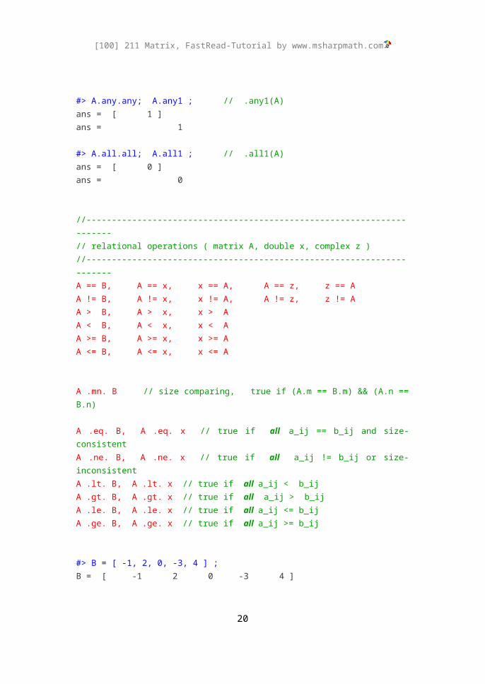
//----------------------------------------------------------------------// relational operations ( matrix A, double x, complex z )//----------------------------------------------------------------------

15


A == B, A == x, x == A, A == z, z == AA != B, A != x, x != A, A != z, z != AA > B, A > x, x > AA < B, A < x, x < AA >= B, A >= x, x >= AA <= B, A <= x, x <= A

A .mn. B // size comparing, true if (A.m == B.m) && (A.n == B.n)

A .eq. B, A .eq. x // true if all a_ij == b_ij and size-consistentA .ne. B, A .ne. x // true if all a_ij != b_ij or size-inconsistentA .lt. B, A .lt. x // true if all a_ij < b_ijA .gt. B, A .gt. x // true if all a_ij > b_ijA .le. B, A .le. x // true if all a_ij <= b_ijA .ge. B, A .ge. x // true if all a_ij >= b_ij

#> B = [ -1, 2, 0, -3, 4 ] ;B = [ -1 2 0 -3 4 ]

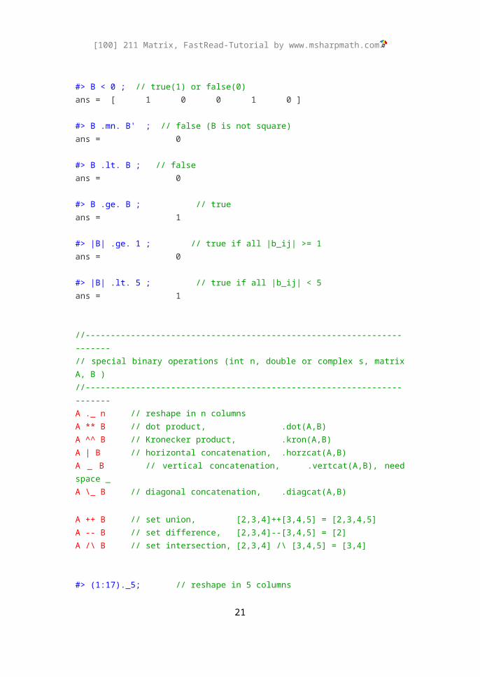
#> B < 0 ; // true(1) or false(0)ans = [ 1 0 0 1 0 ]

#> B .mn. B' ; // false (B is not square)ans = 0

#> B .lt. B ; // falseans = 0

#> B .ge. B ; // trueans = 1

#> |B| .ge. 1 ; // true if all |b_ij| >= 1ans = 0

#> |B| .lt. 5 ; // true if all |b_ij| < 5ans = 1

//----------------------------------------------------------------------// special binary operations (int n, double or complex s, matrix A, B )//----------------------------------------------------------------------A ._ n // reshape in n columnsA ** B // dot product, .dot(A,B)

16


A ^^ B // Kronecker product, .kron(A,B)A | B // horizontal concatenation, .horzcat(A,B)A _ B // vertical concatenation, .vertcat(A,B), need space _A \_ B // diagonal concatenation, .diagcat(A,B) A ++ B // set union, [2,3,4]++[3,4,5] = [2,3,4,5]A -- B // set difference, [2,3,4]--[3,4,5] = [2]A /\ B // set intersection, [2,3,4] /\ [3,4,5] = [3,4]

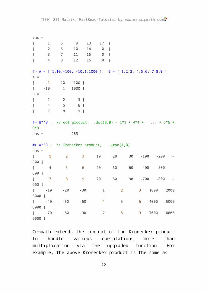
#> (1:17)._5; // reshape in 5 columnsans =[ 1 5 9 13 17 ][ 2 6 10 14 0 ][ 3 7 11 15 0 ][ 4 8 12 16 0 ]

#> A = [ 1,10,-100; -10,1,1000 ]; B = [ 1,2,3; 4,5,6; 7,8,9 ];A =[ 1 10 -100 ][ -10 1 1000 ]B =[ 1 2 3 ][ 4 5 6 ][ 7 8 9 ]

#> B**B ; // dot product, .dot(B,B) = 1*1 + 4*4 + ... + 6*6 + 9*9ans = 285

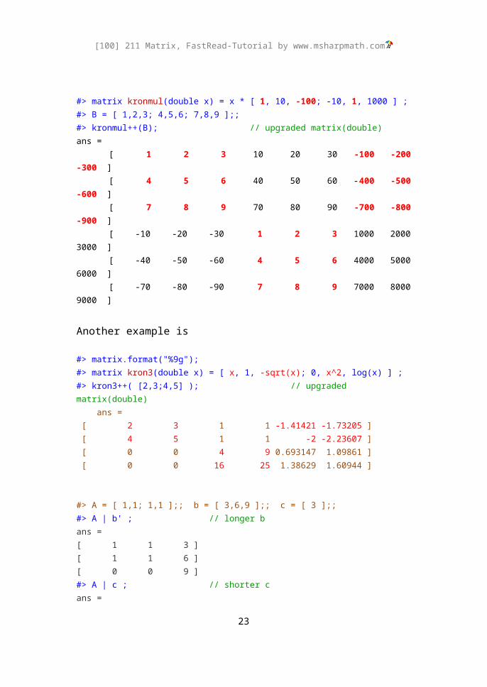
#> A^^B ; // Kronecker product, .kron(A,B)ans =[ 1 2 3 10 20 30 -100 -200 -300 ][ 4 5 6 40 50 60 -400 -500 -600 ][ 7 8 9 70 80 90 -700 -800 -900 ][ -10 -20 -30 1 2 3 1000 2000 3000 ][ -40 -50 -60 4 5 6 4000 5000 6000 ][ -70 -80 -90 7 8 9 7000 8000 9000 ]

Cemmath extends the concept of the Kronecker product to handle various operatations more than multiplication via the upgraded function. For example, the above Kronecker product is the same as

#> matrix kronmul(double x) = x * [ 1, 10, -100; -10, 1, 1000 ] ;#> B = [ 1,2,3; 4,5,6; 7,8,9 ];; #> kronmul++(B); // upgraded matrix(double)

17


ans = [ 1 2 3 10 20 30 -100 -200 -300 ] [ 4 5 6 40 50 60 -400 -500 -600 ] [ 7 8 9 70 80 90 -700 -800 -900 ] [ -10 -20 -30 1 2 3 1000 2000 3000 ] [ -40 -50 -60 4 5 6 4000 5000 6000 ] [ -70 -80 -90 7 8 9 7000 8000 9000 ]

Another example is

#> matrix.format("%9g");#> matrix kron3(double x) = [ x, 1, -sqrt(x); 0, x^2, log(x) ] ; #> kron3++( [2,3;4,5] ); // upgraded matrix(double) ans = [ 2 3 1 1 -1.41421 -1.73205 ] [ 4 5 1 1 -2 -2.23607 ] [ 0 0 4 9 0.693147 1.09861 ] [ 0 0 16 25 1.38629 1.60944 ]

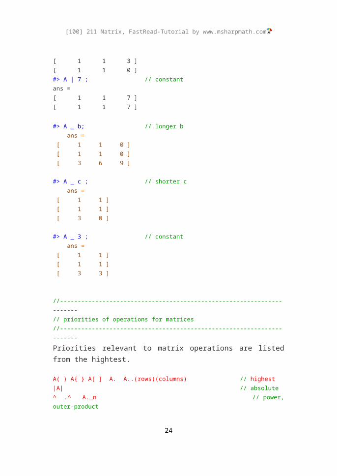
#> A = [ 1,1; 1,1 ];; b = [ 3,6,9 ];; c = [ 3 ];; #> A | b' ; // longer bans =[ 1 1 3 ][ 1 1 6 ][ 0 0 9 ]#> A | c ; // shorter cans =[ 1 1 3 ][ 1 1 0 ]#> A | 7 ; // constantans =[ 1 1 7 ][ 1 1 7 ] #> A _ b; // longer b ans = [ 1 1 0 ] [ 1 1 0 ] [ 3 6 9 ]

#> A _ c ; // shorter c ans = [ 1 1 ] [ 1 1 ]

18


[ 3 0 ]

#> A _ 3 ; // constant ans = [ 1 1 ] [ 1 1 ] [ 3 3 ]

//----------------------------------------------------------------------// priorities of operations for matrices//----------------------------------------------------------------------Priorities relevant to matrix operations are listed from the hightest.

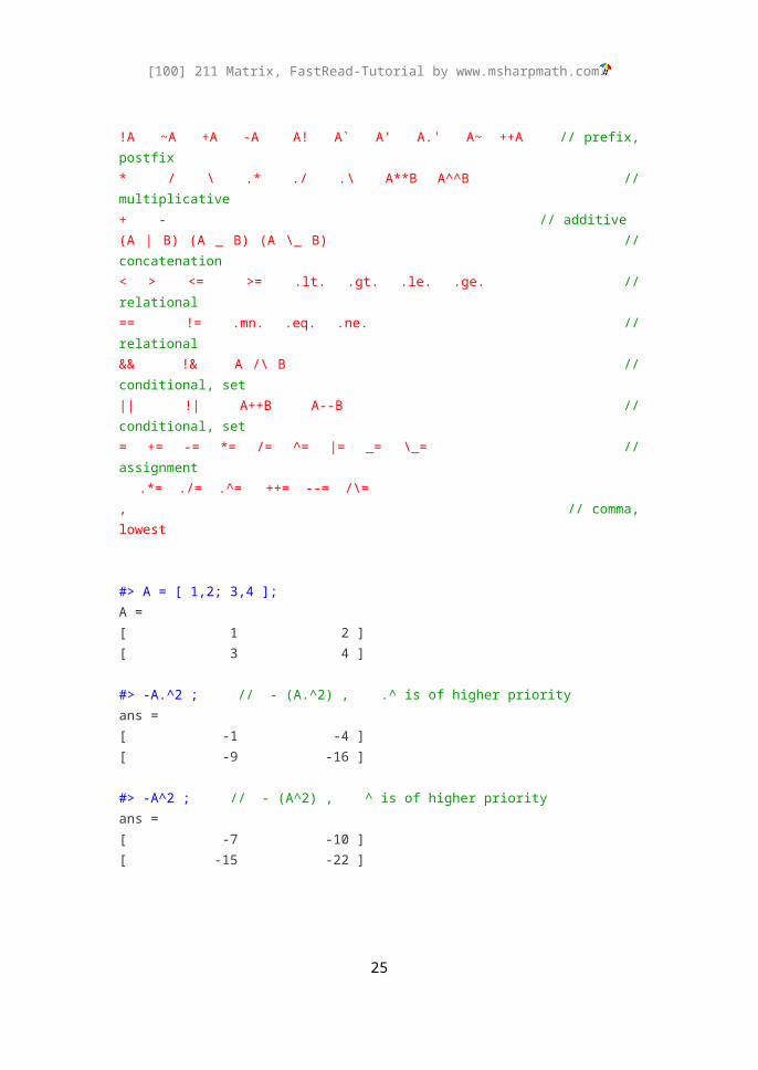
A( ) A{ } A[ ] A. A..(rows)(columns) // highest|A| // absolute^ .^ A._n // power, outer-product!A ~A +A -A A! A` A' A.' A~ ++A // prefix, postfix* / \ .* ./ .\ A**B A^^B // multiplicative+ - // additive(A | B) (A _ B) (A \_ B) // concatenation< > <= >= .lt. .gt. .le. .ge. // relational== != .mn. .eq. .ne. // relational&& !& A /\ B // conditional, set|| !| A++B A--B // conditional, set= += -= *= /= ^= |= _= \_= // assignment

.*= ./= .^= ++= --= /\=, // comma, lowest

#> A = [ 1,2; 3,4 ];A =[ 1 2 ][ 3 4 ]

#> -A.^2 ; // - (A.^2) , .^ is of higher priorityans =[ -1 -4 ][ -9 -16 ]

#> -A^2 ; // - (A^2) , ^ is of higher priorityans =[ -7 -10 ][ -15 -22 ]

19


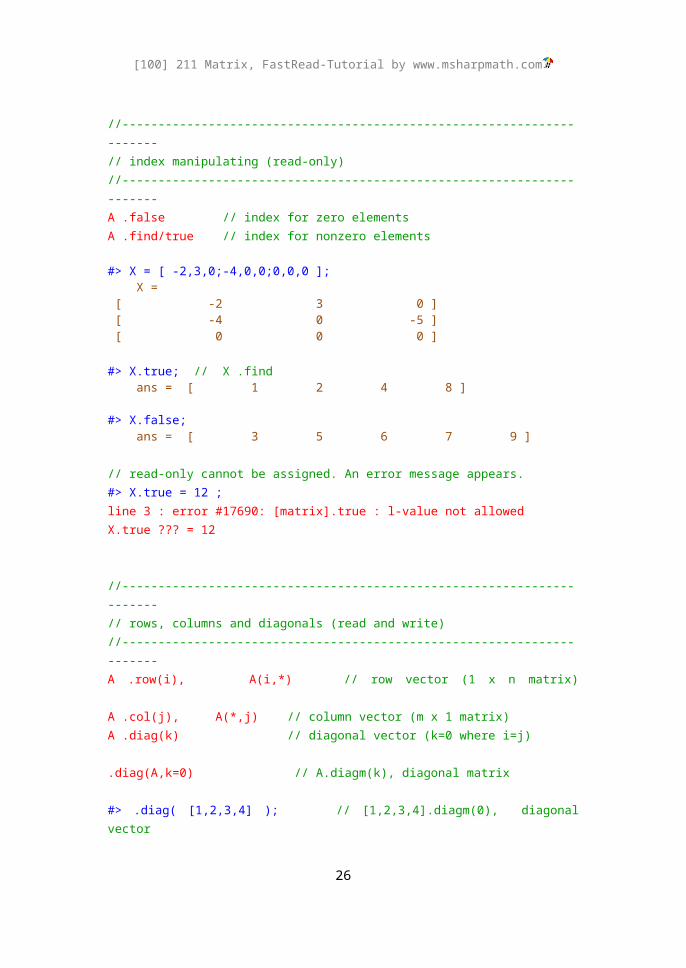
//----------------------------------------------------------------------// index manipulating (read-only)//----------------------------------------------------------------------A .false // index for zero elementsA .find/true // index for nonzero elements

#> X = [ -2,3,0;-4,0,0;0,0,0 ]; X = [ -2 3 0 ] [ -4 0 -5 ] [ 0 0 0 ]

#> X.true; // X .find ans = [ 1 2 4 8 ]

#> X.false; ans = [ 3 5 6 7 9 ]

// read-only cannot be assigned. An error message appears.#> X.true = 12 ; line 3 : error #17690: [matrix].true : l-value not allowedX.true ??? = 12

//----------------------------------------------------------------------// rows, columns and diagonals (read and write)//----------------------------------------------------------------------A .row(i), A(i,*) // row vector (1 x n matrix) A .col(j), A(*,j) // column vector (m x 1 matrix) A .diag(k) // diagonal vector (k=0 where i=j)

.diag(A,k=0) // A.diagm(k), diagonal matrix

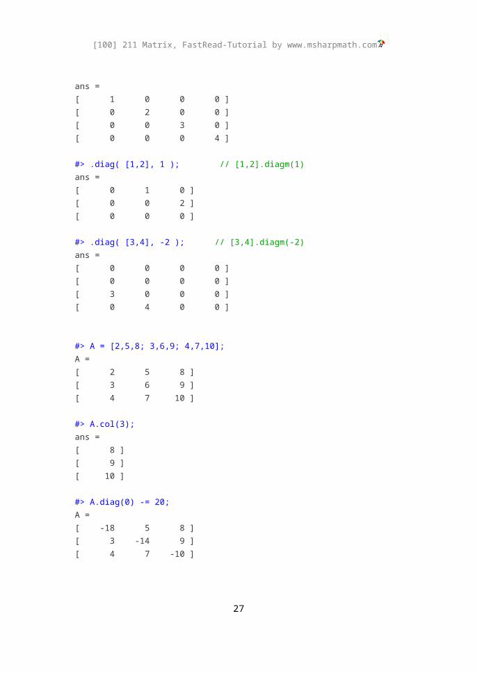
#> .diag( [1,2,3,4] ); // [1,2,3,4].diagm(0), diagonal vectorans =[ 1 0 0 0 ][ 0 2 0 0 ][ 0 0 3 0 ][ 0 0 0 4 ]

#> .diag( [1,2], 1 ); // [1,2].diagm(1)ans =[ 0 1 0 ][ 0 0 2 ][ 0 0 0 ]

20


#> .diag( [3,4], -2 ); // [3,4].diagm(-2)ans =[ 0 0 0 0 ][ 0 0 0 0 ][ 3 0 0 0 ][ 0 4 0 0 ]

#> A = [2,5,8; 3,6,9; 4,7,10];A =[ 2 5 8 ][ 3 6 9 ][ 4 7 10 ]

#> A.col(3); ans =[ 8 ][ 9 ][ 10 ]

#> A.diag(0) -= 20; A =[ -18 5 8 ][ 3 -14 9 ][ 4 7 -10 ]

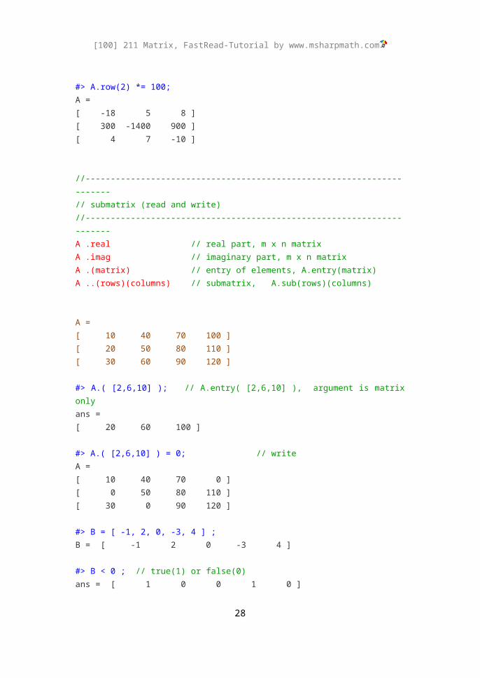
#> A.row(2) *= 100; A =[ -18 5 8 ][ 300 -1400 900 ][ 4 7 -10 ]

//----------------------------------------------------------------------// submatrix (read and write)//----------------------------------------------------------------------A .real // real part, m x n matrixA .imag // imaginary part, m x n matrixA .(matrix) // entry of elements, A.entry(matrix)A ..(rows)(columns) // submatrix, A.sub(rows)(columns)

A =[ 10 40 70 100 ][ 20 50 80 110 ][ 30 60 90 120 ]

21


#> A.( [2,6,10] ); // A.entry( [2,6,10] ), argument is matrix onlyans =[ 20 60 100 ]

#> A.( [2,6,10] ) = 0; // writeA =[ 10 40 70 0 ][ 0 50 80 110 ][ 30 0 90 120 ]

#> B = [ -1, 2, 0, -3, 4 ] ;B = [ -1 2 0 -3 4 ]

#> B < 0 ; // true(1) or false(0)ans = [ 1 0 0 1 0 ]

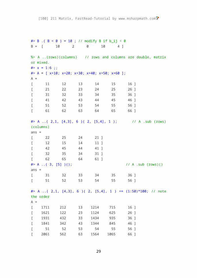
#> B .( B < 0 ) = 10 ; // modify B if b_ij < 0B = [ 10 2 0 10 4 ]

%> A ..(rows)(columns) // rows and columns are double, matrix or mixed.#> x = 1:6 ;;#> A = [ x+10; x+20; x+30; x+40; x+50; x+60 ];A =[ 11 12 13 14 15 16 ][ 21 22 23 24 25 26 ][ 31 32 33 34 35 36 ][ 41 42 43 44 45 46 ][ 51 52 53 54 55 56 ][ 61 62 63 64 65 66 ]

#> A ..( 2,1, [4,3], 6 )( 2, [5,4], 1 ); // A .sub (rows)(columns)ans =[ 22 25 24 21 ][ 12 15 14 11 ][ 42 45 44 41 ][ 32 35 34 31 ][ 62 65 64 61 ]#> A ..( 3, [5] )(); // A .sub (rows)()ans =[ 31 32 33 34 35 36 ][ 51 52 53 54 55 56 ]

#> A ..( 2,1, [4,3], 6 )( 2, [5,4], 1 ) += (1:50)*100; // note the orderA =[ 1711 212 13 1214 715 16 ]

22


[ 1621 122 23 1124 625 26 ][ 1931 432 33 1434 935 36 ][ 1841 342 43 1344 845 46 ][ 51 52 53 54 55 56 ][ 2061 562 63 1564 1065 66 ]

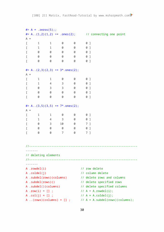
#> A = .zeros(5);;#> A..(1,2)(1,2) += .ones(2); // connecting one pointA =[ 1 1 0 0 0 ][ 1 1 0 0 0 ][ 0 0 0 0 0 ][ 0 0 0 0 0 ][ 0 0 0 0 0 ]

#> A..(2,3)(2,3) += 3*.ones(2);A =[ 1 1 0 0 0 ][ 1 4 3 0 0 ][ 0 3 3 0 0 ][ 0 0 0 0 0 ][ 0 0 0 0 0 ]

#> A..(3,5)(3,5) += 7*.ones(2);A =[ 1 1 0 0 0 ][ 1 4 3 0 0 ][ 0 3 10 0 7 ][ 0 0 0 0 0 ][ 0 0 7 0 7 ]

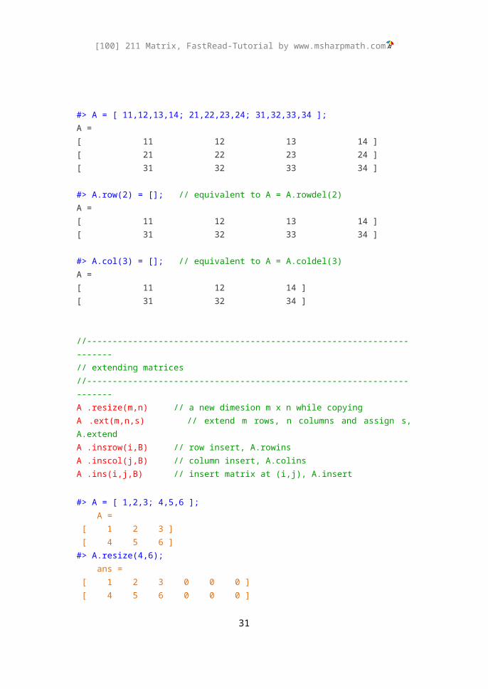
//----------------------------------------------------------------------// deleting elements//----------------------------------------------------------------------A .rowdel(i) // row deleteA .coldel(j) // column deleteA .subdel(rows)(columns) // delete rows and columnsA .subdel(rows)() // delete specified rowsA .subdel()(columns) // delete specified columnsA .row(i) = [] ; // A = A.rowdel(i);A .col(j) = [] ; // A = A.coldel(j);A ..(rows)(columns) = [] ; // A = A.subdel(rows)(columns);

23


#> A = [ 11,12,13,14; 21,22,23,24; 31,32,33,34 ];A =[ 11 12 13 14 ][ 21 22 23 24 ][ 31 32 33 34 ]

#> A.row(2) = []; // equivalent to A = A.rowdel(2)A =[ 11 12 13 14 ][ 31 32 33 34 ]

#> A.col(3) = []; // equivalent to A = A.coldel(3)A =[ 11 12 14 ][ 31 32 34 ]

//----------------------------------------------------------------------// extending matrices//----------------------------------------------------------------------A .resize(m,n) // a new dimesion m x n while copyingA .ext(m,n,s) // extend m rows, n columns and assign s, A.extend A .insrow(i,B) // row insert, A.rowinsA .inscol(j,B) // column insert, A.colinsA .ins(i,j,B) // insert matrix at (i,j), A.insert

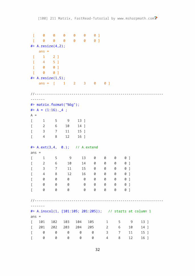
#> A = [ 1,2,3; 4,5,6 ]; A = [ 1 2 3 ] [ 4 5 6 ]#> A.resize(4,6); ans = [ 1 2 3 0 0 0 ] [ 4 5 6 0 0 0 ] [ 0 0 0 0 0 0 ] [ 0 0 0 0 0 0 ]#> A.resize(4,2); ans = [ 1 2 ] [ 4 5 ] [ 0 0 ] [ 0 0 ]#> A.resize(1,5); ans = [ 1 2 3 0 0 ]

24


//----------------------------------------------------------------------#> matrix.format("%6g");#> A = (1:16)._4 ; A =[ 1 5 9 13 ][ 2 6 10 14 ][ 3 7 11 15 ][ 4 8 12 16 ]

#> A.ext(3,4, 0.); // A.extendans =[ 1 5 9 13 0 0 0 0 ][ 2 6 10 14 0 0 0 0 ][ 3 7 11 15 0 0 0 0 ][ 4 8 12 16 0 0 0 0 ][ 0 0 0 0 0 0 0 0 ][ 0 0 0 0 0 0 0 0 ][ 0 0 0 0 0 0 0 0 ]

//----------------------------------------------------------------------#> A.inscol(1, [101:105; 201:205]); // starts at column 1ans =[ 101 102 103 104 105 1 5 9 13 ][ 201 202 203 204 205 2 6 10 14 ][ 0 0 0 0 0 3 7 11 15 ][ 0 0 0 0 0 4 8 12 16 ]

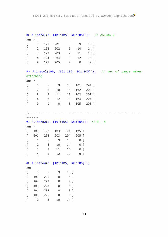
#> A.inscol(2, [101:105; 201:205]'); // column 2ans =[ 1 101 201 5 9 13 ][ 2 102 202 6 10 14 ][ 3 103 203 7 11 15 ][ 4 104 204 8 12 16 ][ 0 105 205 0 0 0 ]

#> A.inscol(100, [101:105; 201:205]'); // out of range makes attachingans =[ 1 5 9 13 101 201 ][ 2 6 10 14 102 202 ][ 3 7 11 15 103 203 ][ 4 8 12 16 104 204 ][ 0 0 0 0 105 205 ]

//----------------------------------------------------------------------#> A.insrow(1, [101:105; 201:205]); // B _ Aans =

25


[ 101 102 103 104 105 ][ 201 202 203 204 205 ][ 1 5 9 13 0 ][ 2 6 10 14 0 ][ 3 7 11 15 0 ][ 4 8 12 16 0 ]

#> A.insrow(2, [101:105; 201:205]');ans =[ 1 5 9 13 ][ 101 201 0 0 ][ 102 202 0 0 ][ 103 203 0 0 ][ 104 204 0 0 ][ 105 205 0 0 ][ 2 6 10 14 ][ 3 7 11 15 ][ 4 8 12 16 ]

#> A.insrow(100, [101:105; 201:205]'); // A _ Bans =[ 1 5 9 13 ][ 2 6 10 14 ][ 3 7 11 15 ][ 4 8 12 16 ][ 101 201 0 0 ][ 102 202 0 0 ][ 103 203 0 0 ][ 104 204 0 0 ][ 105 205 0 0 ]

//----------------------------------------------------------------------#> A.ins(1,1, [101:105; 201:205]);ans =[ 101 102 103 104 105 0 0 0 0 ][ 201 202 203 204 205 0 0 0 0 ][ 0 0 0 0 0 1 5 9 13 ][ 0 0 0 0 0 2 6 10 14 ][ 0 0 0 0 0 3 7 11 15 ][ 0 0 0 0 0 4 8 12 16 ]

#> A.ins(2,2, [101:105; 201:205]');ans =[ 1 0 0 5 9 13 ][ 0 101 201 0 0 0 ][ 0 102 202 0 0 0 ]

26


[ 0 103 203 0 0 0 ][ 0 104 204 0 0 0 ][ 0 105 205 0 0 0 ][ 2 0 0 6 10 14 ][ 3 0 0 7 11 15 ][ 4 0 0 8 12 16 ]

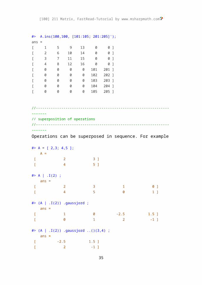
#> A.ins(100,100, [101:105; 201:205]');ans =[ 1 5 9 13 0 0 ][ 2 6 10 14 0 0 ][ 3 7 11 15 0 0 ][ 4 8 12 16 0 0 ][ 0 0 0 0 101 201 ][ 0 0 0 0 102 202 ][ 0 0 0 0 103 203 ][ 0 0 0 0 104 204 ][ 0 0 0 0 105 205 ]

//----------------------------------------------------------------------// superposition of operations//----------------------------------------------------------------------Operations can be superposed in sequence. For example

#> A = [ 2,3; 4,5 ]; A = [ 2 3 ] [ 4 5 ]

#> A | .I(2) ; ans = [ 2 3 1 0 ] [ 4 5 0 1 ]

#> (A | .I(2)) .gaussjord ; ans = [ 1 0 -2.5 1.5 ] [ 0 1 2 -1 ]

#> (A | .I(2)) .gaussjord ..()(3,4) ; ans = [ -2.5 1.5 ] [ 2 -1 ]

27


#> (A | .I(2)) .gaussjord ..()(3,4).ratio; (1/2) x [ -5 3 ] [ 4 -2 ]

//----------------------------------------------------------------------// 'figure'-Returning Functions//----------------------------------------------------------------------A .plot // plotA .splplot // plot piecewise polynomials

//----------------------------------------------------------------------// piecewise polynomials//----------------------------------------------------------------------Piecewise continuous polynomials are defined with a number of polynomials and corresponding intervals

x11≤x ≤x12 : p1 ( x )=a10+a11 x+a12 x2+…+a1n x

n+…x21≤ x≤ x22 : p2 ( x )=a20+a21 x+a22 x

2+…+a2n xn+…

⋮

xm1≤ x≤ xm2: pm ( x )=am0+am1 x+am2 x2+…+amn x

n+…

Combination of these piecewise polynomials can be expressed by the following matrix

A=[ x11 x12 a10 a11 ⋯x21 x22 a20 a21 ⋯⋮ ⋮ ⋮ ⋮ ⋮xm1 xm2 am 0 am1 ⋯ ]

This special representation by a matrix can be handled in various ways

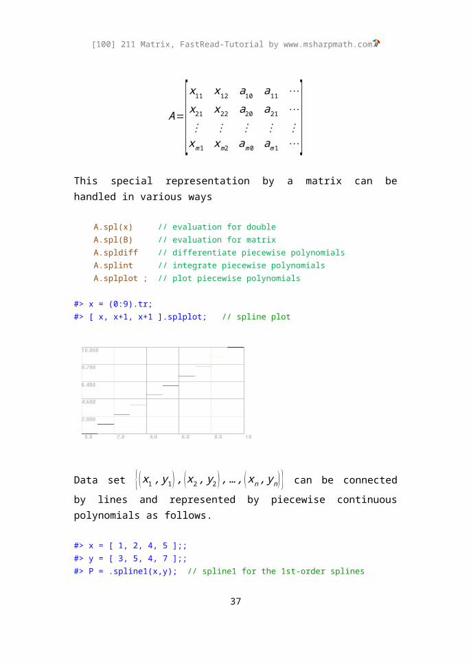
A.spl(x) // evaluation for double A.spl(B) // evaluation for matrix A.spldiff // differentiate piecewise polynomials A.splint // integrate piecewise polynomials A.splplot ; // plot piecewise polynomials

#> x = (0:9).tr;

28


#> [ x, x+1, x+1 ].splplot; // spline plot

Data set {( x1 , y1) , (x2 , y2 ) ,…, (xn, yn )} can be connected by lines and represented by piecewise continuous polynomials as follows.

#> x = [ 1, 2, 4, 5 ];; #> y = [ 3, 5, 4, 7 ];; #> P = .spline1(x,y); // spline1 for the 1st-order splines P = [ 1 2 1 2 ] [ 2 4 6 -0.5 ] [ 4 5 -8 3 ]

1≤x ≤2 : p1 ( x )=1+2 x2≤x ≤4 : p2 (x )=6−0.5x4 ≤x ≤5 : p3 ( x )=−8+3 x

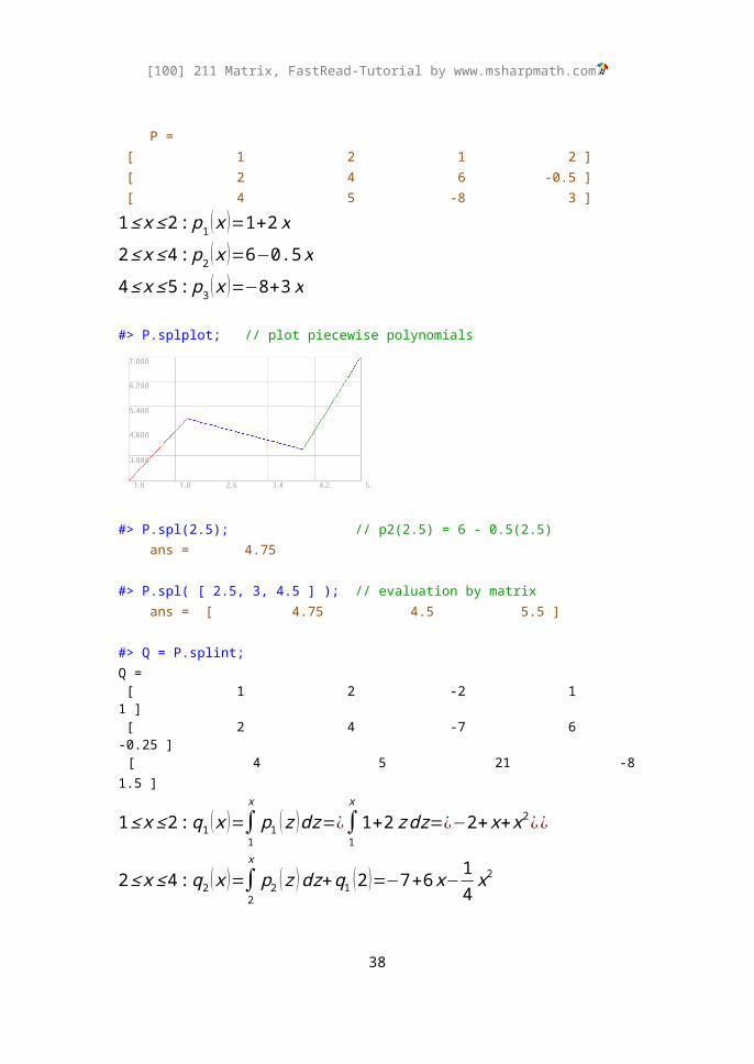
#> P.splplot; // plot piecewise polynomials

#> P.spl(2.5); // p2(2.5) = 6 - 0.5(2.5) ans = 4.75

#> P.spl( [ 2.5, 3, 4.5 ] ); // evaluation by matrix

29


ans = [ 4.75 4.5 5.5 ]

#> Q = P.splint; Q = [ 1 2 -2 1 1 ] [ 2 4 -7 6 -0.25 ] [ 4 5 21 -8 1.5 ]

1≤x ≤2 :q1 ( x )=∫1

x

p1 (z ) dz=¿∫1

x

1+2 z dz=¿−2+x+x2 ¿¿

2≤x ≤4 :q2 ( x )=∫2

x

p2 ( z )dz+q1 (2 )=−7+6 x−14x2

4 ≤x ≤5 :q3 ( x )=∫4

x

p3 ( z ) dz+q2 (4 )=21−8x+ 32x2

#> Q.spl(4.5) - Q.spl(2.5); ans = 8.9375

∫2.5

4

p2 (x )dx+∫4

4.5

p3 ( x )dx=[−7+6x−14x2]

2.5

4

+[21−8 x+32x2]

4

4.5

=8.9375

For spline interpolation using 3rd-degree polynomials, example is

#> x = [ 1, 2, 4, 5 ];; #> y = [ 3, 5, 4, 7 ];; #> P = .spline(x,y); // 1st and 2nd columns for interval P = [ 1 2 1 0.625 2.0625 -0.6875 ] [ 2 4 -10.5 17.875 -6.5625 0.75 ] [ 4 5 89.5 -57.125 12.1875 -0.8125 ]

1≤x ≤2 : p1 ( x )=1+0.625 x+2.0625 x2−0.6875 x3

2≤x ≤4 : p2 (x )=−10.5+17.875 x−6.5625 x2+0.75 x3

4 ≤x ≤5 : p3 ( x )=89.5−57.125 x+12.1875 x2−0.8125 x3

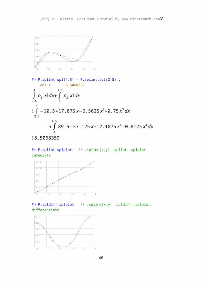
#> P.splplot; // .spline(x,y).splplot;#> [ x', y' ].plot+ ;

30


#> P.splint.spl(4.5) - P.splint.spl(2.5) ; ans = 8.5068359

∫2.5

4

p2 (x )dx+∫4

4.5

p3 ( x )dx

¿∫2.5

4

−10.5+17.875 x−6.5625 x2+0.75x3dx

+∫4

4.5

89.5−57.125 x+12.1875 x2−0.8125 x3dx

¿8.5068359

#> P.splint.splplot; // .spline(x,y) .splint .splplot; integrate

#> P.spldiff.splplot; // .spline(x,y) .spldiff .splplot; differentiate

//----------------------------------------------------------------------// 'poly'-Returning Functions

31


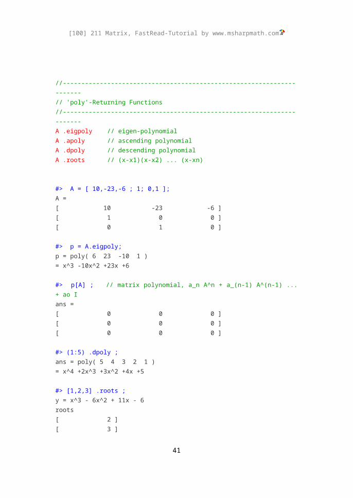
//----------------------------------------------------------------------A .eigpoly // eigen-polynomialA .apoly // ascending polynomialA .dpoly // descending polynomialA .roots // (x-x1)(x-x2) ... (x-xn)

#> A = [ 10,-23,-6 ; 1; 0,1 ];A =[ 10 -23 -6 ][ 1 0 0 ][ 0 1 0 ]

#> p = A.eigpoly;p = poly( 6 23 -10 1 )= x^3 -10x^2 +23x +6

#> p[A] ; // matrix polynomial, a_n A^n + a_(n-1) A^(n-1) ... + ao Ians =[ 0 0 0 ][ 0 0 0 ][ 0 0 0 ]

#> (1:5) .dpoly ;ans = poly( 5 4 3 2 1 )= x^4 +2x^3 +3x^2 +4x +5

#> [1,2,3] .roots ;y = x^3 - 6x^2 + 11x - 6roots[ 2 ][ 3 ][ 1 ]local maxima ( 1.42265, 0.3849 )local minima ( 2.57735, -0.3849 )inflection pt. ( 2, 0 )y-axis intersect ( 0, -6 )

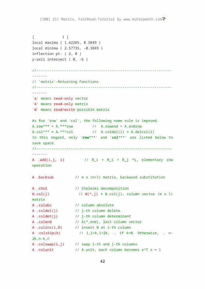
//----------------------------------------------------------------------// 'matrix'-Returning Functions//----------------------------------------------------------------------'a' means read-only vector'A' means read-only matrix'W' means read/write possible matrix

As for 'row' and 'col', the following name rule is imposed.

32


A.row*** = A.***row // A.rowend = A.endrowA.col*** = A.***col // A.coldel(i) = A.delcol(i)In this regard, only 'row***' and 'col***' are listed below to save space.//----------------------------------------------------------------------A .add(i,j, s) // R_i = R_i + R_j *s, elementary row operation

A .backsub // n x (n+1) matrix, backward substitution

A .chol // Choleski decompositionW.col(j) // W(*,j) = W.col(j), column vector (m x 1) matrixA .colabs // column absoluteA .coldel(j) // j-th column deleteA .coldet(j) // j-th column determinantA .colend // A(*,end), last column vectorA .colins(i,B) // insert B at i-th columnA .colskip(k) // 1,1+k,1+2k, .. if k>0. Otherwise, .. n-2k,n-k,nA .colswap(i,j) // swap i-th and j-th columnsA .colunit // A.unit, each column becomes x^T x = 1A .conj // ~A = A.conj, complex conjugateA .conjtr // A' = A.conjtr, conjugate transposeA .cumprod // cumulative product (column-first)A .cumsum // A~ = A.cumsum, cumulative sum (column-first)

A .decimal // deviation from closest interger A .dfact // element-by-element double factorialW.diag(k) // diagonal vector (k=0 where i=j)A .diagm(k) // .diag(A,k) for vectors, otherwise all-zero off-diagsA .diff // A` = A.diff, finite-difference (column-first)

A .eig // eigenvalues vector A .eigvec(lam) // eigenvector corresponding to lamW.entry(matrix) // entry of elements, W.(matrix)A .ext(ni,nj,s) // extend ni rows, nj columns and assign s

A .fact // element-by-element factorialA .false // index for zero elementsA .find // A.true = A.find, index for nonzero elementsA .fliplr // reverse columns, flip left-rightA .flipud // reverse rows, flip upside-downA .forsub // n x (n+1) matrix, forward substitution

A .gausselim // Gauss-elimination without pivotA .gaussjord // Gauss-Jordan elimination with pivotA .gausspivot // Gauss-elimination with pivot

33


A .hess // eigenvalue-preserving Hessenberg matrixA .high(m) // reshape in m-row matrix

W.imag // imaginary part, m x n matrixA .ins(i,j,B) // insert matrix B at (i,j)A .inv // inverse matrix

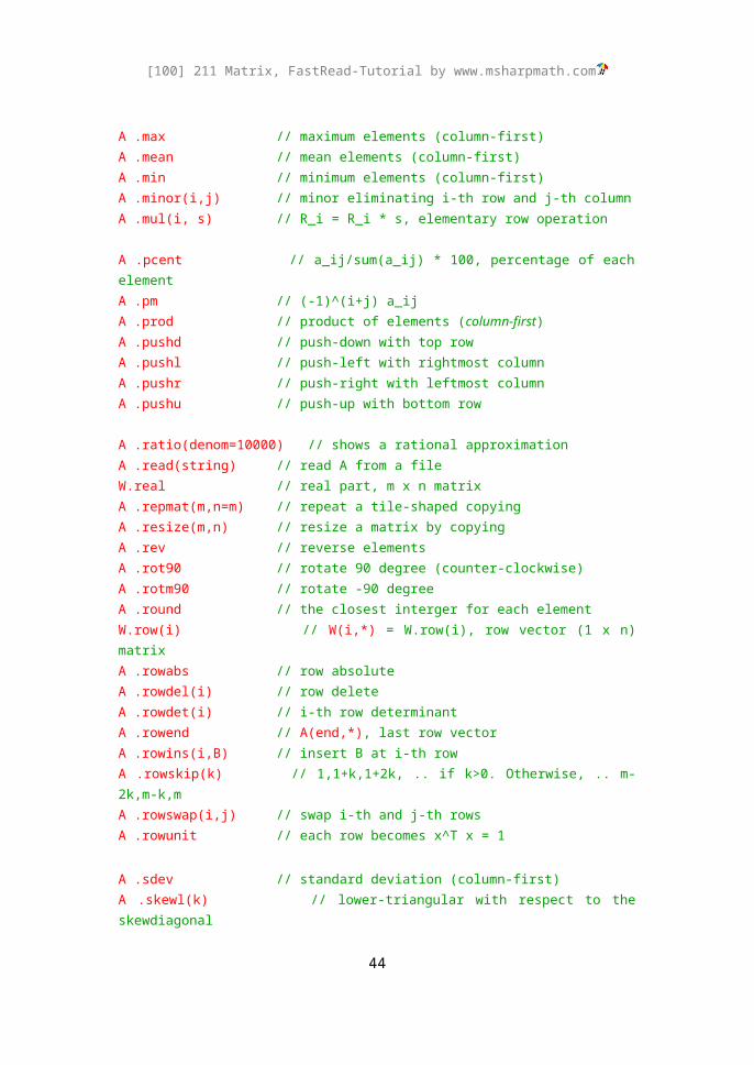
A .max // maximum elements (column-first)A .mean // mean elements (column-first)A .min // minimum elements (column-first)A .minor(i,j) // minor eliminating i-th row and j-th columnA .mul(i, s) // R_i = R_i * s, elementary row operation

A .pcent // a_ij/sum(a_ij) * 100, percentage of each elementA .pm // (-1)^(i+j) a_ijA .prod // product of elements (column-first)A .pushd // push-down with top row A .pushl // push-left with rightmost columnA .pushr // push-right with leftmost columnA .pushu // push-up with bottom row

A .ratio(denom=10000) // shows a rational approximationA .read(string) // read A from a fileW.real // real part, m x n matrixA .repmat(m,n=m) // repeat a tile-shaped copyingA .resize(m,n) // resize a matrix by copyingA .rev // reverse elementsA .rot90 // rotate 90 degree (counter-clockwise)A .rotm90 // rotate -90 degreeA .round // the closest interger for each elementW.row(i) // W(i,*) = W.row(i), row vector (1 x n) matrixA .rowabs // row absoluteA .rowdel(i) // row deleteA .rowdet(i) // i-th row determinantA .rowend // A(end,*), last row vectorA .rowins(i,B) // insert B at i-th row A .rowskip(k) // 1,1+k,1+2k, .. if k>0. Otherwise, .. m-2k,m-k,mA .rowswap(i,j) // swap i-th and j-th rowsA .rowunit // each row becomes x^T x = 1

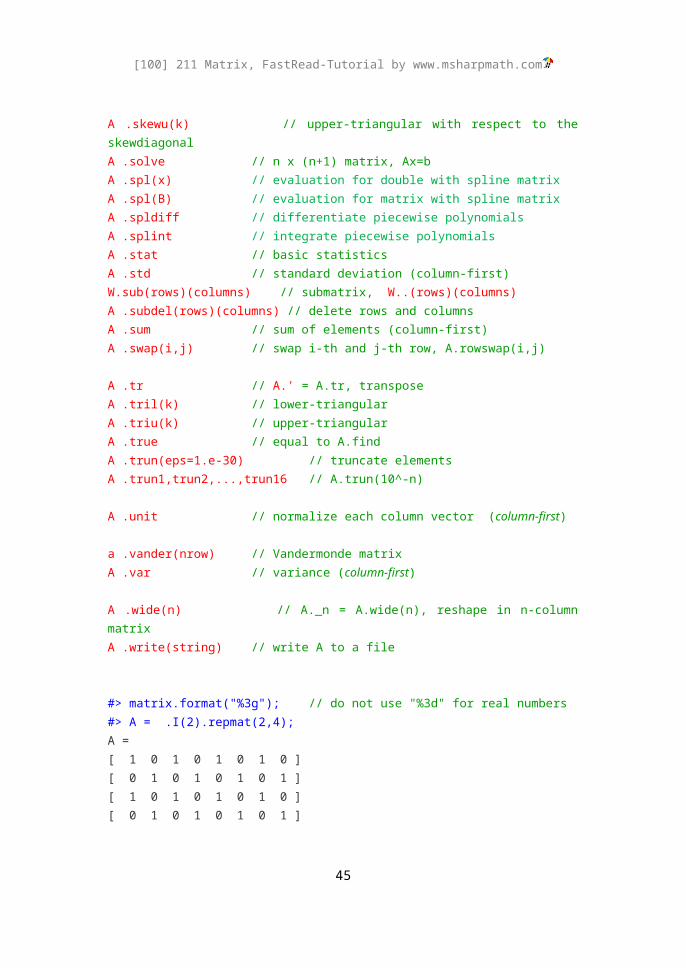
A .sdev // standard deviation (column-first)A .skewl(k) // lower-triangular with respect to the skewdiagonalA .skewu(k) // upper-triangular with respect to the skewdiagonalA .solve // n x (n+1) matrix, Ax=bA .spl(x) // evaluation for double with spline matrix

34


A .spl(B) // evaluation for matrix with spline matrixA .spldiff // differentiate piecewise polynomialsA .splint // integrate piecewise polynomialsA .stat // basic statisticsA .std // standard deviation (column-first)W.sub(rows)(columns) // submatrix, W..(rows)(columns)A .subdel(rows)(columns) // delete rows and columnsA .sum // sum of elements (column-first)A .swap(i,j) // swap i-th and j-th row, A.rowswap(i,j)

A .tr // A.' = A.tr, transposeA .tril(k) // lower-triangularA .triu(k) // upper-triangularA .true // equal to A.findA .trun(eps=1.e-30) // truncate elementsA .trun1,trun2,...,trun16 // A.trun(10^-n)

A .unit // normalize each column vector (column-first)

a .vander(nrow) // Vandermonde matrixA .var // variance (column-first)

A .wide(n) // A._n = A.wide(n), reshape in n-column matrixA .write(string) // write A to a file

#> matrix.format("%3g"); // do not use "%3d" for real numbers#> A = .I(2).repmat(2,4);A =[ 1 0 1 0 1 0 1 0 ][ 0 1 0 1 0 1 0 1 ][ 1 0 1 0 1 0 1 0 ][ 0 1 0 1 0 1 0 1 ]

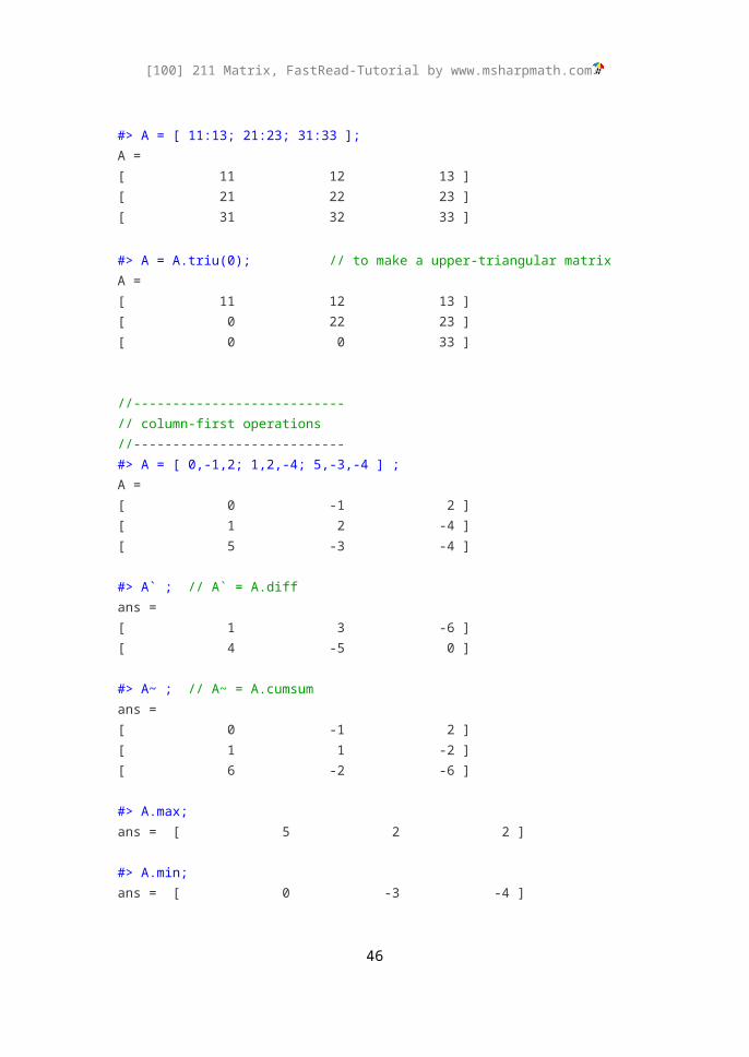
#> A = [ 11:13; 21:23; 31:33 ];A =[ 11 12 13 ][ 21 22 23 ][ 31 32 33 ]

#> A = A.triu(0); // to make a upper-triangular matrixA =[ 11 12 13 ][ 0 22 23 ][ 0 0 33 ]

35


//---------------------------// column-first operations//---------------------------#> A = [ 0,-1,2; 1,2,-4; 5,-3,-4 ] ;A =[ 0 -1 2 ][ 1 2 -4 ][ 5 -3 -4 ]

#> A` ; // A` = A.diffans =[ 1 3 -6 ][ 4 -5 0 ]

#> A~ ; // A~ = A.cumsumans =[ 0 -1 2 ][ 1 1 -2 ][ 6 -2 -6 ]

#> A.max;ans = [ 5 2 2 ]

#> A.min;ans = [ 0 -3 -4 ]

#> A.sum;ans = [ 6 -2 -6 ]

#> A.mean;ans = [ 2 -0.666667 -2 ]

#> A.sdev;ans = [ 2.16025 2.0548 2.82843 ]

#> A.std;ans = [ 2.64575 2.51661 3.4641 ]

#> A.var;ans = [ 7 6.33333 12 ]

#> A.prod;ans = [ 0 6 32 ]

36


#> A.cumprod;ans =[ 0 -1 2 ][ 0 -2 -8 ][ 0 6 32 ]

#> A .unit;ans =[ 0 -0.267261 0.333333 ][ 0.196116 0.534522 -0.666667 ][ 0.980581 -0.801784 -0.666667 ]

//----------------------------------------------------------------------// 'double'-Returning Functions//----------------------------------------------------------------------

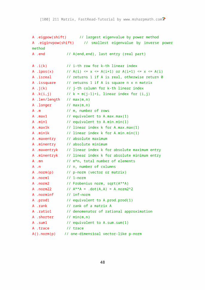
A .cond // condition number, A.norminf*A.inv.norminfA .det // determinantA .eigpow(shift) // largest eigenvalue by power methodA .eiginvpow(shift) // smallest eigenvalue by inverse power methodA .end // A(end,end), last entry (real part)

A .i(k) // i-th row for k-th linear indexA .ipos(x) // A(i) <= x <= A(i+1) or A(i+1) <= x <= A(i)A .isreal // returns 1 if A is real, otherwise return 0A .issquare // returns 1 if A is square n x n matrixA .j(k) // j-th column for k-th linear indexA .k(i,j) // k = m(j-1)+i, linear index for (i,j)A .len/length // max(m,n)A .longer // max(m,n)A .m // m, number of rowsA .max1 // equivalent to A.max.max(1)A .min1 // equivalent to A.min.min(1)A .max1k // linear index k for A.max.max(1)A .min1k // linear index k for A.min.min(1)A .maxentry // absolute maximumA .minentry // absolute minimumA .maxentryk // linear index k for absolute maximum entryA .minentryk // linear index k for absolute minimum entryA .mn // m*n, total number of elementsA .n // n, number of columnsA .norm(p) // p-norm (vector or matrix)A .norm1 // 1-normA .norm2 // Frobenius norm, sqrt(A**A)

37


A .norm22 // A**A = .dot(A,A) = A.norm2^2 A .norminf // inf-normA .prod1 // equivalent to A.prod.prod(1)A .rank // rank of a matrix AA .ratio1 // denomenator of rational approximationA .shorter // min(m,n)A .sum1 // equivalent to A.sum.sum(1)A .trace // trace A().norm(p) // one-dimensioal vector-like p-norm

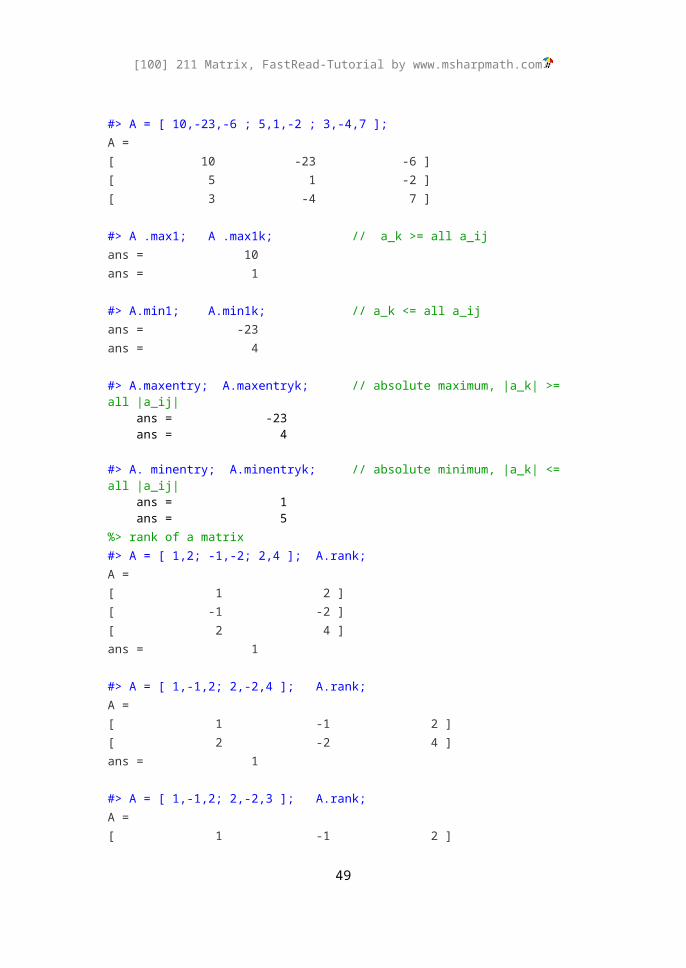
#> A = [ 10,-23,-6 ; 5,1,-2 ; 3,-4,7 ];A =[ 10 -23 -6 ][ 5 1 -2 ][ 3 -4 7 ]

#> A .max1; A .max1k; // a_k >= all a_ijans = 10ans = 1

#> A.min1; A.min1k; // a_k <= all a_ijans = -23ans = 4

#> A.maxentry; A.maxentryk; // absolute maximum, |a_k| >= all |a_ij| ans = -23 ans = 4

#> A. minentry; A.minentryk; // absolute minimum, |a_k| <= all |a_ij| ans = 1 ans = 5%> rank of a matrix#> A = [ 1,2; -1,-2; 2,4 ]; A.rank;A =[ 1 2 ][ -1 -2 ][ 2 4 ]ans = 1

#> A = [ 1,-1,2; 2,-2,4 ]; A.rank;A =[ 1 -1 2 ][ 2 -2 4 ]ans = 1

38


#> A = [ 1,-1,2; 2,-2,3 ]; A.rank;A =[ 1 -1 2 ][ 2 -2 3 ]ans = 2

//----------------------------------------------------------------------// 'tuple'-returning functions//----------------------------------------------------------------------(X,D) = A .eig // modal and spectral matrices(lam, X) = A .eigpow(shift) // largest eigenvalue by power method(lam, X) = A .eiginvpow(shift) // smallest eigenvalue by inverse power method(i,j) = A .ij(k) // k = m(j-1)+i, index (i,j) for linear index k(L,U) = A .lu // A = LU decomposition(P,L,U) = A .plu // A = PLU decomposition(Q,R) = A .qr // A = QR decomposition(m,n) = A .size // number of rows and columns

%> case of distinct real eigenvalues ------------------------#> A = [ 3,1,-1; -22,-10,32; -2,-1,3 ];A =[ 3 1 -1 ][ -22 -10 32 ][ -2 -1 3 ]

#> A .eigpoly;ans = poly( -6 1 4 1 )= x^3 +4x^2 +x -6

#> A .eig; // eigenvaluesans =[ -2 ][ -3 ][ 1 ]

#> (X,D) = A .eig;X =[ 24 25 21 ][ -138 -170 -42 ][ -18 -20 0 ]D =

39


[ -2 0 0 ][ 0 -3 0 ][ 0 0 1 ]

#> (X \ A * X) .trun10 ; // similar matrix, X^-1 A Xans =[ -2 0 0 ][ 0 -3 0 ][ 0 0 1 ]

%> case of complex eigenvalues ------------------------#> A = [ -2, 1 ; -5 ];A =[ -2 1 ][ -5 0 ]

#> A.eig; // eigenvaluesans =[ -1 - i 2 ][ -1 + i 2 ]

#> (X,D) = A.eig; // modal and spectral matricesX =[ -1 - i 2 -1 + i 2 ][ -5 -5 ]D =[ -1 - i 2 0 ][ 0 -1 + i 2 ]

//----------------------------------------------------------------------// matrix argument functions//----------------------------------------------------------------------Mathematical functions for matrix are normally carried out in an 'element-by-element' manner. In addition, functions are extended such that

sqrtm(A) from XX = Aexpm(A) = I + A + A^2/2! + A^3/3! + ....logm(A), inverse of expm

In the above, sqrtm(A) is considered to be A^0.5. In this regard, the power of a matrix A^s is extended.

40


#> A = [ 1,0.3; 0.2,1 ]; sqrt(A); X = sqrtm(A);A =[ 1 0.3 ][ 0.2 1 ]ans =[ 1 0.547723 ][ 0447214 1 ]X =[ 0.992355 0.151156 ][ 0.10077 1 ]

#> X^2 ;ans =[ 1 0.3 ][ 0.2 1 ]

#> E = expm(A); L = logm(A);ans =[ 2.80024 0.823664 ][ 0.549109 2.80024 ]ans =[ -0.0309377 0.306226 ][ 0.20415 -0.0309377 ]

#> logm(E); expm(L);ans =[ 1 0.3 ][ 0.2 1 ]ans =[ 1 0.3 ][ 0.2 1 ]

#> B = A^(1/3); B^3 ;B =[ 0.99318 0.101145 ][ 0.06743 0.99318 ]ans =[ 1 0.3 ][ 0.2 1 ]

//----------------------------------------------------------------------// useful dot functions for matrices//----------------------------------------------------------------------A ** B = .dot(A,B) // dot product

41


A ^^ B = .kron(A,B) // kronecker product A | B = .horzcat(A,B) // horizontal concatenation A _ B = .vertcat(A,B) // vertical concatenationA \_ B = .diagcat(A,B) // diagonal concatenation

.cross(A,B) // cross product

Three dot functions are applied to multiple number of arguments such that

.horzcat(A1,A2,A3, ... ) // multiple matrices are concatenated

.vertcat(A1,A2,A3, ... ) // multiple matrices are stacked vertically

.diagcat(A1,A2,A3, ... ) // multiple matrices are stacked diagonally

#> .diagcat(5,6,7,8) ; // block-diagonal blkdiag(...) in matlabans =[ 5 0 0 0 ][ 0 6 0 0 ][ 0 0 7 0 ][ 0 0 0 8 ]

#> .diagcat( [1,2;3,4], 5, [ 11,12 ] ); // block-diagonalans =[ 1 2 0 0 0 ][ 3 4 0 0 0 ][ 0 0 5 0 0 ][ 0 0 0 11 12 ]

#> .diagcat( 2*.I(2), .ones(2) ); // block-diagonalans =[ 2 0 0 0 ][ 0 2 0 0 ][ 0 0 1 1 ][ 0 0 1 1 ]

Most of the above 'dot functions' are multiply defined due to their role of operators.

//----------------------------------------------------------------------// special matrices//----------------------------------------------------------------------matrix .hilb (integer) // Hilbert matrixmatrix .hank (matrix,matrix) // hankelmatrix .toep (matrix,matrix) // toeplitzmatrix .jord (integer,double) // jordan

42


#> matrix.hank ([3,1,2,0],[0,-1,-2,-3]);ans =[ 3 1 2 0 ][ 1 2 0 -1 ][ 2 0 -1 -2 ][ 0 -1 -2 -3 ]

#> matrix.toep ([1,0,-1,-2],[1,2,4,8]);ans =[ 1 2 4 8 ][ 0 1 2 4 ][ -1 0 1 2 ][ -2 -1 0 1 ]

#> matrix.jord (4,1);ans =[ 1 1 0 0 ][ 0 1 1 0 ][ 0 0 1 1 ][ 0 0 0 1 ]

//----------------------------------------------------------------------// matrix array//----------------------------------------------------------------------An array of matrices is defined according to the following syntaxmatrix P[7],Q[21], ... ;where P and Q are the names of arrays. The dimension of an array can be a variable of type 'double'.

#> matrix.format("%3g"); n = 7;;#> matrix Ar[n];#> for.i(0,4) Ar[i] = .I(i+1);;#> Ar;Ar = matrix [7][0] = [ 1 ][1] =[ 1 0 ][ 0 1 ][2] =[ 1 0 0 ][ 0 1 0 ]

43


[ 0 0 1 ][3] =[ 1 0 0 0 ][ 0 1 0 0 ][ 0 0 1 0 ][ 0 0 0 1 ][4] =[ 1 0 0 0 0 ][ 0 1 0 0 0 ][ 0 0 1 0 0 ][ 0 0 0 1 0 ][ 0 0 0 0 1 ][5] =[ undefined ][6] =[ undefined ]

#> Ar[1];ans =[ 1 0 ][ 0 1 ]

#> Ar[4].mn ;ans = 25

#> Ar[5].mn ;ans = 0

//----------------------------------------------------------------------// matrix declaration//----------------------------------------------------------------------matrix [m,n=1] // matrix [m] is equivalent to matrix [m,1]matrix [ A ]matrix [m,n=1] .i .j ( f(i,j) ) // 1 <= i <= m, 1 <= j <= nmatrix [A] .i .j ( f(i,j) )

// 1 <= k <= m*n (column-wise index k = i + (j-1)m)matrix [m,n=1] .k ( f(k) ) matrix [A] .k ( f(k) )

#> A = matrix[3,3] .i.j( 1/(i+j-1) ); // Hilbert matrixA =[ 1 0.5 0.333333 ]

44


[ 0.5 0.333333 0.25 ][ 0.333333 0.25 0.2 ]

#> B = matrix[A] .i.j( exp(-(i+j)/5)*cos(i/3*pi) );B =[ 0.33516 0.274406 0.224664 ][ -0.274406 -0.224664 -0.18394 ][ -0.449329 -0.367879 -0.301194 ]

//----------------------------------------------------------------------// tensor-related functions for stress analysis//----------------------------------------------------------------------A .xrot(theta) // rotation around the x-axisA .yrot(theta) // rotation around the y-axisA .zrot(theta) // rotation around the z-axisA .xrotd(theta) // rotation around the x-axis (in degree)A .yrotd(theta) // rotation around the y-axis (in degree)A .zrotd(theta) // rotation around the z-axis (in degree)

σ=[ i j k ] [σ11 σ12 σ13

σ21 σ22 σ23

σ31 σ32 σ33][ ijk ] ,[ ijk ]=Q [e1

e2

e3]

σ=[e1 e2 e3 ]QT [σ11 σ 12 σ13

σ21 σ 22 σ23

σ31 σ 32 σ33]Q [e1

e2

e3]

~S=QT [ σ11 σ12 σ 13

σ 21 σ22 σ 23

σ 31 σ32 σ 33]Q

// s = ( ij+ji ), pure shear stress#> X = [ 0,1,0; 1,0,0; 0,0,0 ]; X =[ 0 1 0 ][ 1 0 0 ][ 0 0 0 ]

// snew = ( uu-vv ), tension and compression#> X.zrotd(45).trun10;

45


ans =[ 1 0 0 ][ 0 -1 0 ][ 0 0 0 ]

//----------------------------------------------------------------------// geometry-returning functions//----------------------------------------------------------------------[ x1,y1, x2,y2 ].pass ; // a line passing two points[ x1,y1, x2,y2, x3,y3 ].pass ; // a parabola passing three points[ x1,y1, x2,y2, x3,y3, x4,y4 ].pass ; // a cubic passing four points[ x1,y1, x2,y2, x3,y3 ].circle ; // a circle passing three points

#> p = [ -1,-2, 2,3 ] .pass ; // a polynomial for a linep = poly( -0.333333 1.66667 )= 1.66667x -0.333333

#> [ -1,-2, 2,3 ] .pass ; // return a line with informationy = 1.66667x - 0.333333, root = 0.2y = (1/3)*( 5x - 1 )

#> [ -1,2, 2,3, 5,7 ] .pass ; // return a parabola with informationy = 0.166667x^2 + 0.166667x + 2y = (1/6)*( x^2 + x + 12 )roots[ -0.5 - i 3.428 ][ -0.5 + i 3.428 ]vertex at ( -0.5, 1.95833 )y_minimum = 1.95833y-axis intersect ( 0, 2 )symmetry at x = -0.5directrix at y = 0.458333focus at ( -0.5, 3.45833 )

#> [ -1,2, 2,3, 5,7, 8,-1 ] .pass ; // return a cubic with informationy = -0.0925926x^3 + 0.722222x^2 - 0.111111x + 0.740741y = (1/54)*( -5x^3 + 39x^2 - 6x + 40 )roots[ 7.778 ][ 0.01102 - i 1.014 ][ 0.01102 + i 1.014 ]local minima ( 0.078096, 0.736424 )local maxima ( 5.1219, 6.67691 )

46


inflection pt. ( 2.6, 3.70667 )y-axis intersect ( 0, 0.740741 )

// return a matrix for coefficients with information#> [ 1,1, -1,2, 2,4 ] .circle ; circle(-7)(x^2+y^2) + (9)x + (39)y + (-34) = 0center = ( 0.642857, 2.78571 )radius = 1.82108ans = [ -7 9 39 -34 ]

//----------------------------------------------------------------------// application to triangle solution//----------------------------------------------------------------------// lowercase a, b, c for the sides// uppercase A, B, C for the angles[ a, b, c ] .sss // three sides[ a, b, C ] .sas // two sides and in-between angle[ b, C, A ] .asa // one side and two end-angles[ b, A, B ] .saa // one side and two angles[ a, b, A ] .ssa // two sides and one angle[ a, b, c ] .area // area of three-sides triangle

When solution exists, the final result is returned as a 3 x 3 matrix

[ a, b, c ][ A, B, C ][ S, rI, rO ]

In the above,

S is the area of a trianglerI is the radius of incirclerO is the radius of circumcircle

Several functions plot triangles.plot .sss(a, b, c); plot .ssso(a, b, c)plot .sas(a, b, C); plot .saso(a, b, C)plot .asa(b, C, A); plot .asao(b, C, A);plot .saa(b, A, B)plot .ssa(a, b, A)

47


More detailed solutions can be found by

[ a, b, c ] .ssso // three sides[ a, b, C ] .saso // two sides and in-between angle[ b, C, A ] .asao // one side and two end-angles

returns 14 x 3 matrix for triangle properties.

1. [ a, b, c ]2. [ A, B, C ]3. [ S, rI, rO ]4. [ reA, reB, reC ] // radii of 3 excircles5. [ Ax, Ay ] // coordinate of point A6. [ Bx, By ]7. [ Cx, Cy ]8. [ Ix, Iy ] // incenter I9. [ Ox, Oy ] // circumcenter O10. [ eAx, eAy ] // excenter eA opposite to A11. [ eBx, eBy ]12. [ eCx, eCy ]13. [ Hx, Hy ] // orthocenter H14. [ Gx, Gy ] // gravity center G

plot .ssso(1,2,sqrt(3));

#> [ 1,2,sqrt(3) ] .ssso; // three-sides triangle solutions[1] (a,b,c) = (1, 2, 1.73205);[2] (A,B,C) = (30, 90, 60);[3] (S,rI,rO) = (0.866025, 0.366025, 1);[4] (reA,reB,reC) = (0.633975, 2.36603, 1.36603);[5] A = ( 2, 0 );[6] B = ( 0.5, 0.866025 );

48


[7] C = ( 0, 0 );[8] I = ( 0.633975, 0.366025 );[9] O = ( 1, -1.11022e-016 );[10] eA = ( -0.366025, 0.633975 );[11] eB = ( 1.36603, -2.36603 );[12] eC = ( 2.36603, 1.36603 );[13] H = ( 0.5, 0.866025 );[14] G = ( 0.833333, 0.288675 );ans =[ 1 2 1.732 ][ 30 90 60 ][ 0.866 0.366 1 ][ 0.634 2.366 1.366 ][ 2 0 0 ][ 0.5 0.866 0 ][ 0 0 0 ][ 0.634 0.366 0 ][ 1 -1.11e-016 0 ][ -0.366 0.634 0 ][ 1.366 -2.366 0 ][ 2.366 1.366 0 ][ 0.5 0.866 0 ][ 0.8333 0.2887 0 ]//----------------------------------------------------------------------

//----------------------------------------------------------------------// end of file//----------------------------------------------------------------------

49

Documents

· Web viewMatrix Much like available commercial softwares, Cemmath adopts class 'matrix' as the most valueable data structure. For concise explanation, we employ mathematical expression