Viewing & Perspective

CSE167: Computer Graphics

Instructor: Steve Rotenberg

UCSD, Fall 2006

Homogeneous Transformations

1 0 00 1

110001

zyx

zzzyzxzz

yzyyyxyy

xzxyxxxx

z

y

x

zzzz

yyyy

xxxx

z

y

x

vvv

dvcvbvav

dvcvbvav

dvcvbvav

v

v

v

dcba

dcba

dcba

v

v

v

vMv

3D Transformations

So far, we have studied a variety of useful 3D transformations: Rotations Translations Scales Shears Reflections

These are examples of affine transformations These can all be combined into a single 4x4 matrix, with

[0 0 0 1] on the bottom row This implies 12 constants, or 12 degrees of freedom

(DOFs)

ABCD Vectors

We mentioned that the translation information is easily extracted directly from the matrix, while the rotation/scale/shear/reflection information is encoded into the upper 3x3 portion of the matrix

The 9 constants in the upper 3x3 matrix make up 3 vectors called a, b, and c

If we think of the matrix as a transformation from object space to world space, then the a vector is essentially the object’s x-axis transformed into world space, b is its y-axis in world space, and c is its z-axis in world space

d is of course the position in world space.

Example: Yaw

A spaceship is floating out in space, with a matrix W. The pilot wants to turn the ship 10 degrees to the left (yaw). Show how to modify W to achieve this.

Example: Yaw We simply rotate W around its own b vector, using the

‘arbitrary axis rotation’ matrix:

where Ra(a,θ)=

1000

0)1()1()1(

0)1()1()1(

0)1()1()1(

22

22

22

zzxzyyzx

xzyyyzyx

yzxzyxxx

acasacaasacaa

sacaaacasacaa

sacaasacaaaca

WMW

dWTbWRdWTM

.10,.. a

Spaces

So far, we’ve discussed the following spaces Object space (local space) World space (global space) Camera space

Camera Space

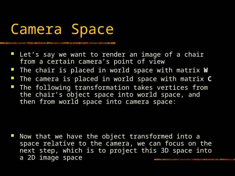
Let’s say we want to render an image of a chair from a certain camera’s point of view

The chair is placed in world space with matrix W The camera is placed in world space with matrix C The following transformation takes vertices from the chair’s object

space into world space, and then from world space into camera space:

Now that we have the object transformed into a space relative to the camera, we can focus on the next step, which is to project this 3D space into a 2D image space

vWCv 1

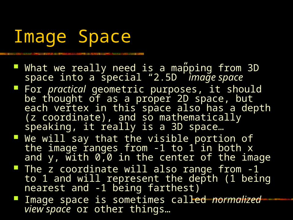
Image Space

What we really need is a mapping from 3D space into a special “2.5D” image space

For practical geometric purposes, it should be thought of as a proper 2D space, but each vertex in this space also has a depth (z coordinate), and so mathematically speaking, it really is a 3D space…

We will say that the visible portion of the image ranges from -1 to 1 in both x and y, with 0,0 in the center of the image

The z coordinate will also range from -1 to 1 and will represent the depth (1 being nearest and -1 being farthest)

Image space is sometimes called normalized view space or other things…

View Projections

So far we know how to transform objects from object space into world space and into camera space

What we need now is some sort of transformation that takes points in 3D camera space and transforms them into our 2.5D image space

We will refer to this class of transformations as view projections (or just projections)

Simple orthographic view projections can just be treated as one more affine transformation applied after the transformation into camera space

More complex perspective projections require a non-affine transformation followed by an additional division to convert from 4D homogeneous space into image space

It is also possible to do more elaborate non-linear projections to achieve fish-eye lens effects, etc., but these require significant changes to the rendering process, not only in the vertex transformation stage, and so we will not cover them…

Orthographic Projection

An orthographic projection is an affine transformation and so it preserves parallel lines

An example of an orthographic projection might be an architect’s top-down view of a house, or a car designer’s side view of a car

These are very valuable for certain applications, but are not used for generating realistic images

Orthographic Projection

1000

200

02

0

002

,,,,,

1

nearfar

nearfar

nearfar

bottomtop

bottomtop

bottomtop

leftright

leftright

leftright

farneartopbottomrightleftorthoP

vWCPv

Perspective Projection

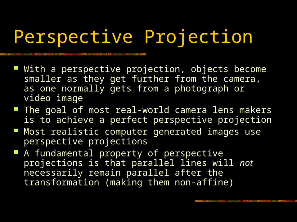
With a perspective projection, objects become smaller as they get further from the camera, as one normally gets from a photograph or video image

The goal of most real-world camera lens makers is to achieve a perfect perspective projection

Most realistic computer generated images use perspective projections

A fundamental property of perspective projections is that parallel lines will not necessarily remain parallel after the transformation (making them non-affine)

View Volume

A camera defines some sort of 3D shape in world space that represents the volume viewable by that camera

For example, a normal perspective camera with a rectangular image describes a sort of infinite pyramid in space

The tip point of the pyramid is at the camera’s origin and the pyramid projects outward in front of the camera into space

In computer graphics, we typically prevent this pyramid from being infinite by chopping it off at some distance from the camera. We refer to this as the far clipping plane

We also put a limit on the closest range of the pyramid by chopping off the tip. We refer to this as the near clipping plane

A pyramid with the tip cut off is known as a frustum. We refer to a standard perspective view volume as a view frustum

View Frustum

In a sense, we can think of this view frustrum as a distorted cube, since it has six faces, each with 4 sides

If we think of this cube as ranging from -1 to 1 in each dimension xyz, we can think of a perspective projection as a mapping from this view frustrum into a normalized view space, or image space

We need a way to represent this transformation mathematically

View Frustum

The view frustum is usually defined by a field of view (FOV) and an aspect ratio, in addition to the near and far clipping plane distances

Depending on the convention, the FOV may represent either the horizontal or vertical field of view. The most common convention is that the FOV is the entire vertical viewing angle

The aspect ratio is the x/y ratio of the final displayed image For example, if we are viewing on a TV that is 24” x 18”, the aspect

ratio would be 24/18 or 4/3 Older style TV’s have a 4/3 aspect ratio, while modern wide screen

TV’s use a 16/9 aspect. These sizes are common for computer monitors as well

Perspective Matrix

0100

200

002/tan

10

0002/tan

,,,

1)4(

farnear

farnear

farnear

farnearfov

aspect

fov

farnearaspectfovpersp

D

P

vWCPv

Perspective Matrix

If we look at the perspective matrix, we see that it doesn’t have [0 0 0 1] on the bottom row

This means that when we transform a 3D position vector [vx vy vz 1], we will not necessarily end up with a 1 in the 4th component of the result vector

Instead, we end up with a true 4D vector [vx′ vy′ vz′ vw′] The final step of perspective projection is to map this 4D

vector back into the 3D w=1 subspace:

w

z

w

y

w

xwzyx v

v

v

v

v

vvvvv

Perspective Transformations

It is important to make sure that straight lines in 3D space map to straight lines in image space

This is easy for x and y, but because of the division, it is possible to have nonlinearities in z

The perspective transformation shown in the previous slide assures a straight line mapping, but there are other perspective transformations possible that don’t preserve this

Viewports

The final transformation takes points from the -1…1 image space and maps them to an actual rectangle of pixels (device coordinates)

We can define our final device mapping from normalized view space into an actual rectangular viewport as:

The depth value is usually mapped to a 32 bit fixed point value ranging from 0 (near) to 0xffffffff (far)

1000

0100

2/02/0

2/002/

,,, 01001

01001

1010

yyyyy

xxxxx

yyxxD

Spaces

Object space (3D) World space (3D) Camera space (3D) Un-normalized view space (4D) Image space (2.5D) Device space (2.5D)

Triangle Rendering

The main stages in the traditional graphics pipeline are: Transform Lighting Clipping / Culling Scan Conversion Pixel Rendering

Transformation

In the transformation stage, vertices are transformed from their original defining object space through a series of steps into a final ‘2.5D’ device space of actual pixels

vDv

v

vWCPv

w

z

w

y

w

x

D

v

v

v

v

v

v

14

Transformation: Step 1

v: The original vertex in object space W: Matrix that transforms object into world space C: Matrix that transforms camera into world space (C-1 will transform

from world space to camera space) P: Non-affine perspective projection matrix v′: Transformed vertex in 4D un-normalized viewing space

Note: sometimes, this step is broken into two (or more) steps. This is often done so that lighting and clipping computations can be done in camera space (before applying the non-affine transformation)

vWCPv 14D

Transformation: Step 2

In the next step, we map points from 4D space into our normalized viewing space, called image space, which ranges from -1 to 1 in x, y, and z

From this point on, we will mainly think of the point as being 2D (x & y) with additional depth information (z). This is sometimes called 2.5D

w

z

w

y

w

x

v

v

v

v

v

vv

Transformation: Step 3

In the final step of the transformation stage, vertices are transformed from the normalized -1…1 image space and mapped into an actual rectangular viewport of pixels

vDv

Transformation

vDv

v

vWCPv

w

z

w

y

w

x

D

v

v

v

v

v

v

14

Matrices in GL

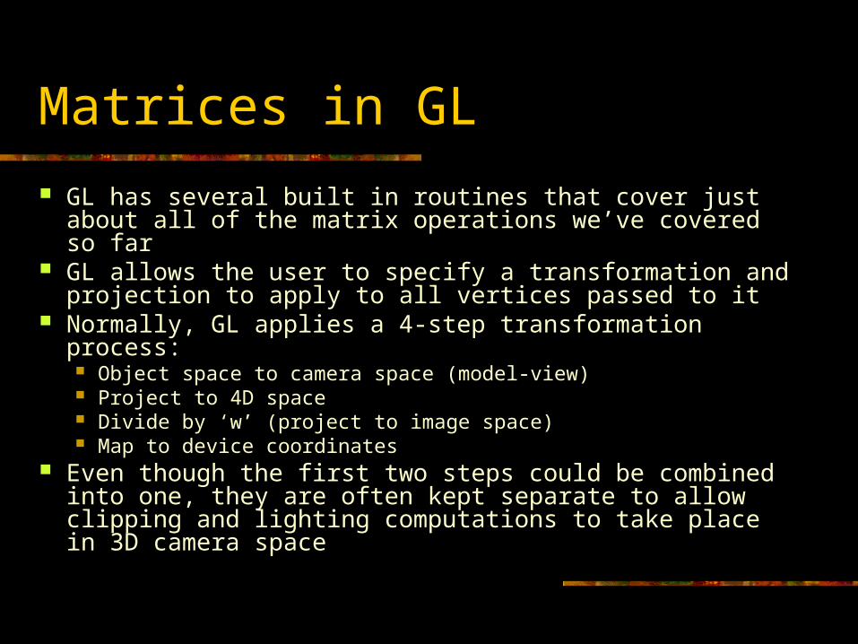
GL has several built in routines that cover just about all of the matrix operations we’ve covered so far

GL allows the user to specify a transformation and projection to apply to all vertices passed to it

Normally, GL applies a 4-step transformation process: Object space to camera space (model-view) Project to 4D space Divide by ‘w’ (project to image space) Map to device coordinates

Even though the first two steps could be combined into one, they are often kept separate to allow clipping and lighting computations to take place in 3D camera space

glMatrixMode()

The glMatrixMode() command allows you to specify which matrix you want to set

At this time, there are two different options we’d be interested in: glMatrixMode(GL_MODELVIEW) glMatrixMode(GL_PROJECTION)

The model-view matrix in GL represents the C-1·W transformation, and the projection matrix is the P matrix

vWCPv 1

glLoadMatrix()

The most direct way to set the current matrix transformation is to use glLoadMatrix() and pass in an array of 16 numbers making up the matrix

Alternately, there is a glLoadIdentity() command for quickly resetting the current matrix back to identity

glRotate(), glTranslate(), glScale()

There are several basic matrix operations that do rotations, translations, and scaling

These operations take the current matrix and modify it by applying the new transformation before the current one, effectively adding a new transformation to the right of the current one

For example, let’s say that our current model-view matrix is called M. If we call glRotate(), the new value for M will be M·R

glPushMatrix(), glPopMatrix()

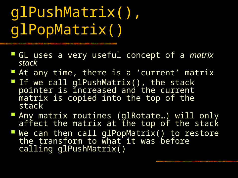
GL uses a very useful concept of a matrix stack At any time, there is a ‘current’ matrix If we call glPushMatrix(), the stack pointer is

increased and the current matrix is copied into the top of the stack

Any matrix routines (glRotate…) will only affect the matrix at the top of the stack

We can then call glPopMatrix() to restore the transform to what it was before calling glPushMatrix()

glFrustum(), gluPerspective()

GL supplies a few functions for specifying the viewing transformation

glFrustum() lets you define the perspective view volume based on actual coordinates of the frustum

glPerspective() gives a more intuitive way to set the perspective transformation by specifying the FOV, aspect, near clip and far clip distances

glOrtho() allows one to specify an orthographic viewing transformation

glLookAt()

glLookAt() implements the ‘look at’ function we covered in the previous lecture

It allows one to specify the camera’s eye point as well as a target point to look at

It also allows one to define the ‘up’ vector, which we previously just assumed would be [0 1 0] (the y-axis)

GL Matrix Example// Clear screenglClear(GL_COLOR_BUFFER_BIT,GL_DEPTH_BUFFER_BIT);

// Set up projectionglMatrixMode(GL_PROJECTION);glLoadIdentity();gluPerspective(fov,aspect,nearclip,farclip);

// Set up camera viewglMatrixMode(GL_MODELVIEW);glLoadIdentity();gluLookAt(eye.x,eye.y,eye.z,target.x,target.y,target.z,0,1,0);

// Draw all objectsfor(each object) {

glPushMatrix();glTranslatef(pos[i].x,pos[i].y,pos[i].z);glRotatef(axis[i].x,axis[i].y,axis[i].z,angle[i]);Model[i]->Draw();glPopMatrix();

}

// FinishglFlush();glSwapBuffers();

Instances

It is common in computer graphics to render several copies of some simpler shape to build up a more complex shape of entire scene

For example, we might render 100 copies of the same chair placed in different positions, with different matrices

We refer to this as object instancing, and a single chair in the above example would be referred to as an instance of the chair model

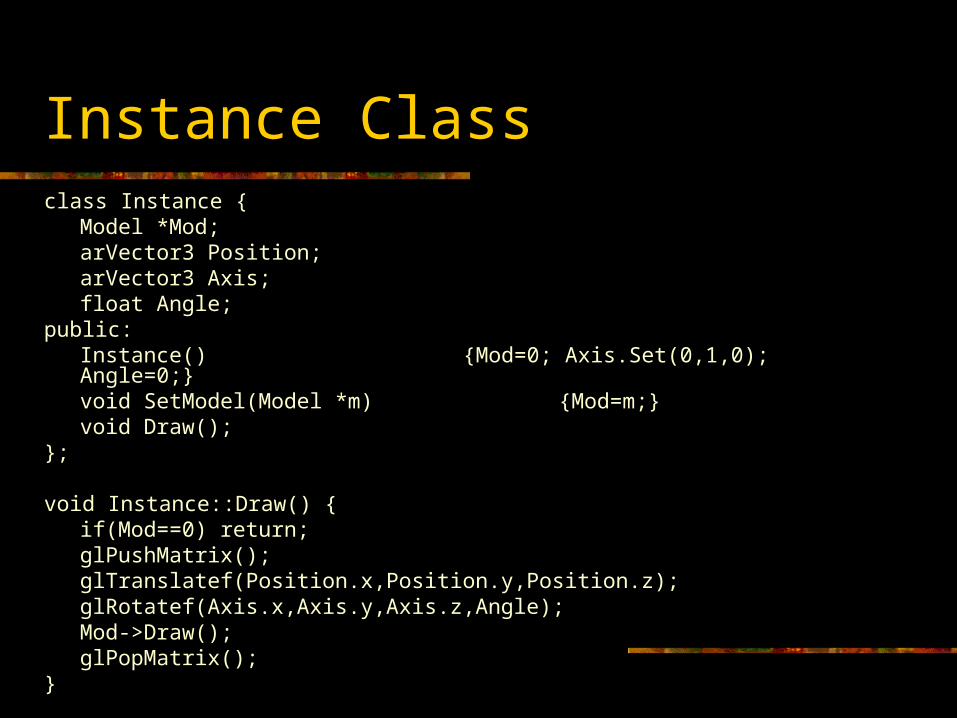
Instance Classclass Instance {

Model *Mod;arVector3 Position;arVector3 Axis;float Angle;

public:Instance() {Mod=0; Axis.Set(0,1,0); Angle=0;}void SetModel(Model *m) {Mod=m;}void Draw();

};

void Instance::Draw() {if(Mod==0) return;glPushMatrix();glTranslatef(Position.x,Position.y,Position.z);glRotatef(Axis.x,Axis.y,Axis.z,Angle);Mod->Draw();glPopMatrix();

}

Camera Class

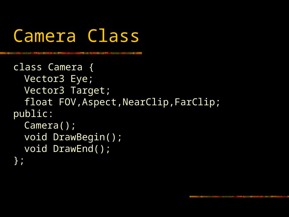
class Camera {Vector3 Eye;Vector3 Target;float FOV,Aspect,NearClip,FarClip;

public:Camera();void DrawBegin();void DrawEnd();

};