Introductionbura.brunel.ac.uk/bitstream/2438/13842/1/Fulltext.docx · Web viewFIRSTRUN – Fiscal Rules and Strategies under Externalities and Uncertainties. Funded by the Horizon

FIRSTRUN – Fiscal Rules and Strategies under Externalities and Uncertainties.Funded by the Horizon 2020 Framework Programme of the European Union.

Project ID 649261.

FIRSTRUN Deliverable 4.7

Macroprudential tools, transmission and modelling

Abstract:The purpose of this paper is twofold. First, we review the theoretical and empirical literature on macroprudential policies and tools. Second, we test empirically the effectiveness of several macroprudential policies and tools using available quarterly datasets from the IMF and BIS that cover up to 19 OECD countries during 2000-2014. Our dataset includes a more detailed set of macroprudential variables compared to the data used by other studies at the cost of narrowing the number of countries covered. In addition, our focus on OECD countries gives us access to a wider range of control variables whose omission may lead to excessively favourable results on the impact of macroprudential policies. We find evidence that macroprudential polices are effective at curbing house price and credit growth, albeit some tools are more effective than others. These include, in particular, taxes on financial institutions and strict loan-to-value and debt-to-income ratio limits.

Keywords: Macroprudential policy, house prices, credit, systemic riskJEL Classification: E58, G28

Authors:1

Oriol Carreras, NIESRE. Philip Davis, NIESR and Brunel UniversityRebecca Piggott, NIESR

Delivery date: 2016-08-31

1 Carreras, NIESR, [email protected], Davis: Visiting Fellow, NIESR and Professor of Banking and Finance, Brunel University. Emails, [email protected] and [email protected], Piggott: NIESR, [email protected]. We thank Ray Barrell, Jagjit Chadha, Simon Kirby, Dennison Noel and participants in a seminar at NIESR as well as Eugenio Cerutti for help and suggestions.

FIRSTRUN (649261)

Table of contents

1 Introduction......................................................................................................................................3

2 Taxonomies and overview of macroprudential policies.....................................................................4

2.1 Taxonomies......................................................................................................................................4

2.2 General macroprudential tools.........................................................................................................5

2.3 Housing market tools: loan-to-value limits.......................................................................................6

2.4 Other sector-specific macroprudential tools....................................................................................7

3 Literature survey on modelling the impact and transmission mechanism of macroprudential policy..8

3.1 Theoretical research papers on macroprudential policy..................................................................8

3.2 Theoretical work on macroprudential and monetary policy.............................................................9

3.3 Datasets for macroprudential research..........................................................................................11

3.4 Empirical research papers on macroprudential policy using global samples..................................14

4 Modelling the impact of macroprudential policies...........................................................................19

5 SUR estimates.................................................................................................................................32

6 Conclusions.....................................................................................................................................44

7 References......................................................................................................................................44

8 Appendix A: selected national experiences of macroprudential policies...........................................49

9 Appendix B: summary of the literature............................................................................................51

10 Appendix C: estimation of equations for spreads.........................................................................55

FIRSTRUN (649261) Deliverable 4.7 2

1 Introduction Macroprudential policy is focused on the financial system as a whole, with a view to limiting macroeconomic costs from financial distress (Crockett 2010), with risk taken as endogenous to the behaviour of the financial system. However, as noted by Galati and Moessner (2014), “analysis is still needed about the appropriate macroprudential tools, their transmission mechanism and their effect”. Theoretical models are in their infancy and empirical evidence on the effects of macroprudential tools is still scarce. Nor has a primary instrument for macroprudential policy emerged. Accordingly, in this paper we seek to address issues in the tools, transmission and modelling of macroprudential policy. The paper is structured as follows:

In Section 2, we look at general macroprudential instruments, notably capital or provisions held by institutions (either in time series or cross section) not specific to sectors they lend to. An example is the countercyclical buffer of 2.5 percentage points for banks, which rises when times are good and falls when they are bad, where the suggestion in Basel Committee (2010) is that such buffers should be calibrated to credit “gaps”.2 Dynamic provisioning across bank balance sheets also fits into this category. These are tools specifically developed to mitigate systemic risk.3 There are additional tools that may be relevant at times such as capital controls and limits on system wide currency mismatches.

We also examine specific tools targeted to sectors such as housing. These were often not originally developed with systemic risk in mind, but can be modified to target systemic risk. Whereas macroprudential surveillance focused on house prices as a key indicator is common across many countries, attempts to regulate house purchase lending were historically less widespread, but is becoming more common in the light of the sub-prime crisis (Davis, Fic and Karim (2011), CGFS (2010), Darbar and Wu (2014)).

In Section 3, we analyse the transmission of macroprudential and its effectiveness in reducing asset prices, credit growth and financial instability generally. We survey both the theoretical and empirical literature on the effectiveness of macroprudential policy. We also highlight analysis of the interaction of macroprudential and monetary policies. And we present information on the main databases of macroprudential policy. Interestingly, from the literature it is often the sector specific tools that are shown to be most effective, although this may be because of longer experience of their use.

This then forms background to our own modelling exercise which is in Section 4. We seek to estimate panel error correction models for house prices and household sector credit, before testing the additional impact of macroprudential policies. We can use appropriate sets of variables in our equations given we focus on the OECD countries that offer comprehensive datasets. We contrast such results with those typical in the literature for global samples, which include mainly economic growth, policy rates and volatility. We find that a number of policies are shown to be effective for restraining house prices and credit.

We implement a seemingly unrelated regression procedure in Section 5 to address a potential concern of weak cointegration underpinning the panel error correction regressions, particularly for house prices, in

2 Like the output gap, the credit gap measure is the distance between credit levels at time t and the long-run trend as (usually) derived using a Hodrick-Prescott filter.3 The Basel approach builds on the historically less interventionist approach of regulators and central banks in OECD countries, who have until recently taken the view that interest rates and individual bank capital regulation are all that is needed for both monetary and financial stability to be maintained.


Section 4. While a country by country approach tackles successfully the concern of lack of cointegration, it has limited scope for econometric inference as the binary nature of the datasets used in this paper become a more taxing feature. Nevertheless, we still find evidence suggesting that macroprudential policies limit house price and credit growth.

2 Taxonomies and overview of macroprudential policies

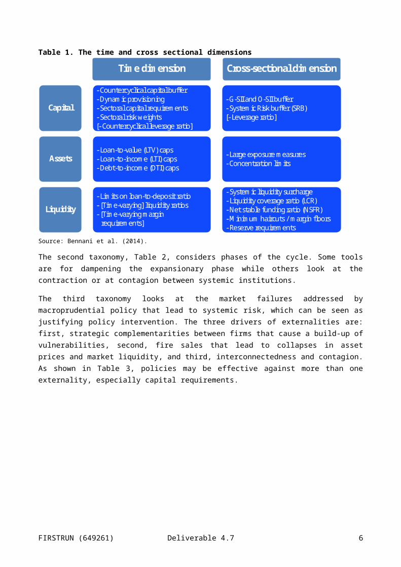
2.1 TaxonomiesGeneral versus specific is not the only possible taxonomy of macroprudential tools. There are also tools that focus on addressing the time dimension (procyclicality) versus the cross sectional dimension, within which there are tools to target capital, assets and liquidity, as shown below in Table 1.

Table 1. The time and cross sectional dimensions

Capital

Assets

Liquidity

Time dimension

- Countercyclical capital buffer- Dynamic provisioning- Sectoral capital requirements- Sectoral risk weights[- Countercyclical leverage ratio]

- Loan-to-value (LTV) caps- Loan-to-income (LTI) caps- Debt-to-income (DTI) caps

- Limits on loan-to-deposit ratio- [Time-varying] liquidity ratios- [Time-varying margin

requirements]

Cross-sectional dimension

- G-SII and O-SII buffer- Systemic Risk buffer (SRB)[- Leverage ratio]

- Large exposure measures- Concentration limits

- Systemic liquidity surcharge- Liquidity coverage ratio (LCR)- Net stable funding ratio (NSFR)- Minimum haircuts / margin floors- Reserve requirements

Source: Bennani et al. (2014).

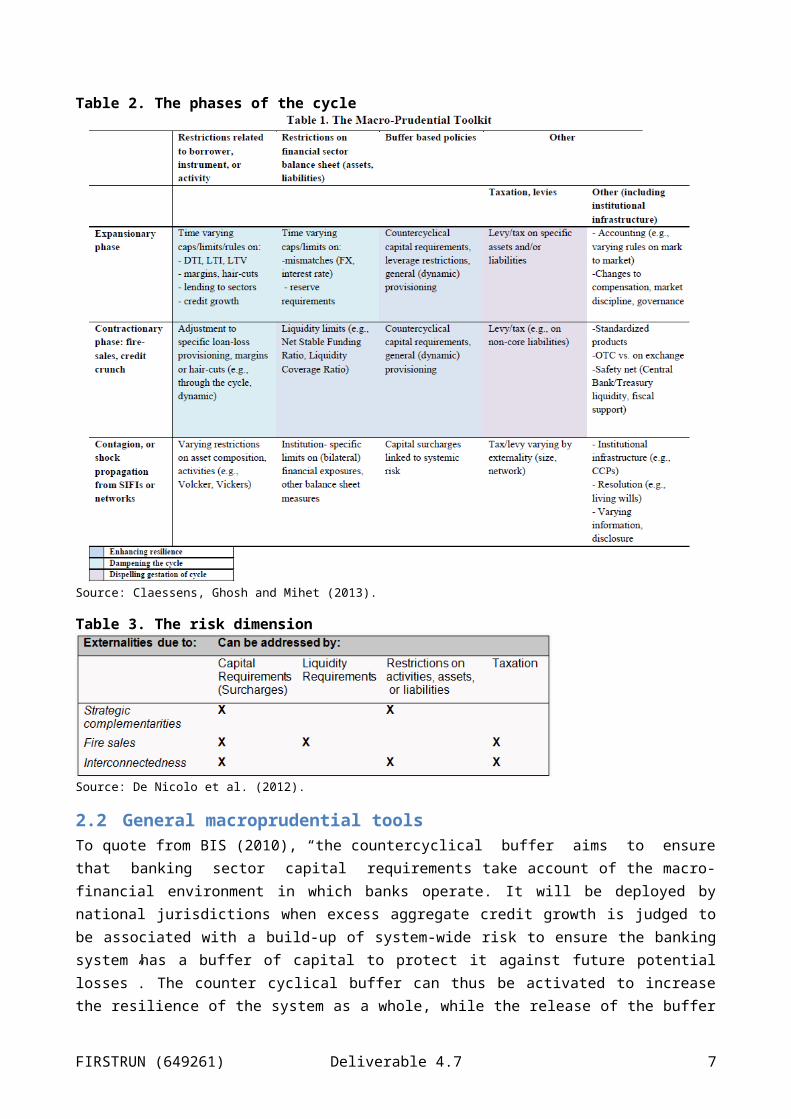
The second taxonomy, Table 2, considers phases of the cycle. Some tools are for dampening the expansionary phase while others look at the contraction or at contagion between systemic institutions.

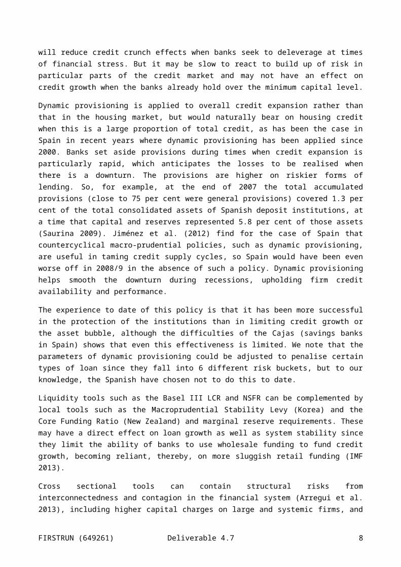
The third taxonomy looks at the market failures addressed by macroprudential policy that lead to systemic risk, which can be seen as justifying policy intervention. The three drivers of externalities are: first, strategic complementarities between firms that cause a build-up of vulnerabilities, second, fire sales that lead to collapses in asset prices and market liquidity, and third, interconnectedness and contagion. As shown in Table 3, policies may be effective against more than one externality, especially capital requirements.


Table 2. The phases of the cycle

Source: Claessens, Ghosh and Mihet (2013).

Table 3. The risk dimension

Source: De Nicolo et al. (2012).

2.2 General macroprudential toolsTo quote from BIS (2010), “the countercyclical buffer aims to ensure that banking sector capital requirements take account of the macro-financial environment in which banks operate. It will be deployed by national jurisdictions when excess aggregate credit growth is judged to be associated with a build-up of system-wide risk to ensure the banking system has a buffer of capital to protect it against future potential losses”. The counter cyclical buffer can thus be activated to increase the resilience of the system as a whole, while the release of the buffer will reduce credit crunch effects when banks seek to deleverage at times of financial stress. But it may be slow to react to build up of risk in particular parts of the credit market and may not have an effect on credit growth when the banks already hold over the minimum capital level.


Dynamic provisioning is applied to overall credit expansion rather than that in the housing market, but would naturally bear on housing credit when this is a large proportion of total credit, as has been the case in Spain in recent years where dynamic provisioning has been applied since 2000. Banks set aside provisions during times when credit expansion is particularly rapid, which anticipates the losses to be realised when there is a downturn. The provisions are higher on riskier forms of lending. So, for example, at the end of 2007 the total accumulated provisions (close to 75 per cent were general provisions) covered 1.3 per cent of the total consolidated assets of Spanish deposit institutions, at a time that capital and reserves represented 5.8 per cent of those assets (Saurina 2009). Jiménez et al. (2012) find for the case of Spain that countercyclical macro-prudential policies, such as dynamic provisioning, are useful in taming credit supply cycles, so Spain would have been even worse off in 2008/9 in the absence of such a policy. Dynamic provisioning helps smooth the downturn during recessions, upholding firm credit availability and performance.

The experience to date of this policy is that it has been more successful in the protection of the institutions than in limiting credit growth or the asset bubble, although the difficulties of the Cajas (savings banks in Spain) shows that even this effectiveness is limited. We note that the parameters of dynamic provisioning could be adjusted to penalise certain types of loan since they fall into 6 different risk buckets, but to our knowledge, the Spanish have chosen not to do this to date.

Liquidity tools such as the Basel III LCR and NSFR can be complemented by local tools such as the Macroprudential Stability Levy (Korea) and the Core Funding Ratio (New Zealand) and marginal reserve requirements. These may have a direct effect on loan growth as well as system stability since they limit the ability of banks to use wholesale funding to fund credit growth, becoming reliant, thereby, on more sluggish retail funding (IMF 2013).

Cross sectional tools can contain structural risks from interconnectedness and contagion in the financial system (Arregui et al. 2013), including higher capital charges on large and systemic firms, and tools to limit large exposures within the financial system. Payments and settlements systems can be adjusted to reduce the risk of a build-up of credit exposures within the financial system.

2.3 Housing market tools: loan-to-value limitsHistorically, use of the loan-to-value (LTV) ratio has been most common in terms of macroprudential tools for the housing market. This has been used in particular in Asian and Eastern European countries (Borio and Shim (2007), Davis, Fic and Karim (2011)). More recently they have been increasingly employed by EU countries. These limits tend to start from a typical “normal” level in the economy from a microprudential point of view, such as 80 per cent. Then they would impose a tightening beyond that of 10 or 20 percentage points. Such limits have historically tended to be chosen in economies that had a heavy exposure to financial cycles and housing markets that responded strongly to credit availability. Often fixed exchange rates would limit the use of monetary policy. LTVs might be complemented by other policies which seek to ensure prudent lending, such as limits on loan to income (these are preferred to LTV by Barrell, Kirby and Whitworth (2011)) and loan concentration, as discussed below. LTVs aim to enhance financial sector resilience and lean against build-ups of risk both at micro and macro levels. Authorities using them typically see them as both effective quantitatively and expressing a helpful signal of concern.

A risk with an LTV cap is to make the maximum level also a minimum and thus raise the LTVs on new lending. On the other hand, there is a risk that LTV limits are circumvented by strategies such as offshore borrowing, unsecured borrowing, financial engineering, falsification of asset valuation or other borrowing


from outside the regulated financial system. Such problems could in principle be avoided by simply making the portion of loans above a regulatory limit non-enforceable in the case of default (Weale 2008) – a policy that has not been tried, to our knowledge, at present.

As for other macroprudential policies, effectiveness of LTV policies is not easy to distinguish from the effects of monetary policy, confidence and income growth expectations upon changes in borrowing and house prices, although the panel econometrics reported in this paper and other studies seeks to overcome this problem. Writing at an early stage, CGFS (2010) seems to suggest that the success in generating resilience has been greater than in restraining credit expansion. In addition, it should be noted that LTV limits are not strictly countercyclical since the ratio depends on an endogenous variable (house prices). Structural features of the financial markets may also limit lending via LTVs, for example in Germany via Pfandbriefe which can only be used to securitise if they have LTVs of less than 80 per cent.

2.4 Other sector-specific macroprudential toolsLTV limits are not the only form of regulation of the terms of credit that can be applied to the housing market. Debt service/income caps have also been tried in a number of countries, notably in East Asia. Such limits require there to be sufficient information exchange between banks and/or the existence of a central credit register.

Some countries have explicitly varied capital weights to allow for concerns regarding the housing market. This enables banks to choose whether or not to lend to the sector judged to be growing too rapidly in the light of the amended cost of lending. They could react by absorbing the cost, raising more capital, and raising the cost of lending to the sector. At a macroeconomic level, it could be seen as widening the spread of mortgage loans over the deposit rate in the housing market, as the deposit margin can also be adjusted when capital requirements are raised (see Barrell et al. 2009). For example, as noted by McCauley (2009), varying capital weights was an instrument used by the Indian central bank in late 2004, raising Basel 1 weights on mortgages and other household credit given rapid economic growth. More recently Brazil and Turkey have imposed capital weights on mortgage and unsecured consumer lending (IMF 2013).

However, Acharya (2013) finds that risk weights imposed to achieve macroprudential goals can instead lead to the build-up of financial risks because risk weights on certain asset classes such as mortgages encourage the build-up of exposure to other assets that are not deemed as risky, but that can contribute to vulnerability with concentrated exposure. Such limits can be conditional on LTVs as cited by McCauley (2009), in that the Reserve Bank of Australia permitted the 50 per cent weight on mortgages to be applied only to loans with an LTV of below 70 per cent.

Implicit taxation of credit growth via reserve requirements was applied widely in the pre-liberalisation policies in countries such as the UK and France, where rapid growth in lending attracted higher reserve requirements on the funding side. In Finland in the late 1980s there was a threshold set on loan growth with lending above that level attracting higher reserve requirements. This was considered successful in restraining lending growth relative to that in Sweden (Berg 1993), although it did not prevent the occurrence of a banking crisis in Finland. Such policies are at times applied to the housing market. Banks with access to securities borrowing or foreign bank credit could avoid such restrictions if imposed on purely domestic lending growth. A response may be direct limits on growth of domestic and/or foreign currency loans.


Loan concentration limits at a sectoral level were applied in Ireland in the late 1990s, which meant that only up to 200 per cent of own-funds could be lent to a given industrial sector, while only up to 250 per cent could be lent to two sectors, which shared the economic risks of an asymmetric shock, such as property and construction. But these evidently did not prevent sufficiently large exposures to lead to economic and financial difficulties in that country. Such limits may also be applied to interbank lending.

3 Literature survey on modelling the impact and transmission mechanism of macroprudential policy

3.1 Theoretical research papers on macroprudential policyWe note there are rather few papers that have sought to look at monetary and macroprudential policy together. These are typically in stylised calibrated models rather than estimated ones (Section 3.2). And a comment from one such paper is relevant “within a standard macroeconomic framework, it is very difficult to derive a satisfactory way of modelling macroprudential objectives” (Angelini et al. 2010).

Galati and Moessner (2014) give a helpful breakdown of progress in macroprudential modelling, into three areas: banking/finance models, three-period banking or DSGE models, and infinite horizon general equilibrium models, which we follow in this paper.

Banking/finance models, in the tradition of Diamond and Dybvig (1983) highlight how financial contracts are affected by various incentive problems related to information asymmetry and commitment that can entail default. Then, there can be self-fulfilling equilibria generated by shocks, leading to systemic financial instability. They accordingly seek to explain the interaction of borrowers and lenders. For example, Perotti and Suarez (2011) look at price based and quantity based regulation of systemic externalities arising from banks’ short term funding. Accordingly, current liquidity regulation could be justified, together with a Pigovian tax on short term funding. However, such models tend to be cross section and omit the time series dimension and thus cannot be used to address procyclicality. Furthermore, they tend to be partial equilibrium and thus omit key general equilibrium effects.

Such effects are included in three period general equilibrium models of the interaction of asset prices and non-financial and financial sector systemic risk. Such models assess risk taking by heterogeneous agents in an economy vulnerable to such systemic risks. For example there may be financial amplification during booms and busts that have external effects as in Goodhart et al. (2012) and Gersbach and Rochet (2012a and b). Individual agents take decisions without allowing for the general equilibrium effects of their actions, in particular the effects of asset sales caused by excessive borrowing on asset prices. Accordingly, they generate patterns of feedback loops entailing falling asset prices, financial constraints and fire sales. Then, macroprudential tools can be shown as helpful in preventing fire sales and credit crunches, including LTV, capital requirements, liquidity coverage rations, dynamic loss provisioning and margin limits on repos by shadow banks (Goodhart et al. 2013).

Further results of interest are provided by models that focus on the functions of banks in the economy such as improving liquidity insurance, risk sharing and raising funding, which as shown by Kashyap et al. (2014) can then be used to analyse weaknesses underlying the global financial crisis, notably excessive risk taking by underfunded banks relying on short term funding and exploiting the safety net. Horvath and Wagner (2013) meanwhile show that new regulations can lead savers and banks to alter other portfolio choices.


Countercyclical regulation can worsen cross sectional risk for example, although tools to reduce cross sectional risk may reduce procyclicality.

Infinite horizon DSGE models with financial frictions build on the insights of papers such as Bernanke et al. (1999) on the financial accelerator. Such models (e.g. Goodfriend and McCallum 2007) were traditionally linear, so found it hard to deal with non-linearities implicit in systemic risk and changes in regulation. They tended to assume complete markets and that defaults either do not occur or are exogenous. And furthermore they tended to ignore endogenous leverage. So a crisis is modelled as a big negative shock that gets amplified rather than a credit boom that gets out of control (Boissay et al. 2013).

More recent models have sought to overcome these problems, with multiple equilibria, non-linearity, externalities and amplification mechanisms being more sophisticated. Hence macroprudential policies can be better assessed, although the models have to remain small due to the difficulty of the solution methods Galati and Moessner (2014). Borrowers may, for example, face occasional binding endogenous borrowing constraints in times of crisis as in Fisher’s (1933) debt deflation paradigm, linked to falling asset prices and declining net worth. See for example Benigno et al. (2013). Meanwhile models such as Brunnermeier and Sannikov (2014) look at global dynamics in continuous time models with financial frictions. The financial sector does not internalise the costs associated with excessive risks, so there is high leverage and maturity mismatch. Securitisation allows risk to be offloaded by the financial sector but raises overall risk taking. The economy has low volatility and adequate growth in steady state but the steady state is unstable due to large shocks provoking endogenous leverage and risk taking with feedback loops from the financial to the real economy. The model features a pattern of rising leverage and amplification when aggregate risk declines, as in the great moderation.

He and Krishnamurthy (2014) have developed a quantitative model to assess the different dynamics in tranquil times and times of stress. Benes et al. (2014) provide a simulation model where parameters are calibrated to the features of financial cycles.

In general, such models highlight the transmission mechanism of real and financial factors, with the combination of macroeconomic boom, credit boom and low interest rates being dangerous, with consumption smoothing and precautionary saving being key underlying factors in financial imbalances’ build-up. Model calibrations can help with understanding how macroprudential regulation can reduce the risk of crisis. State contingent taxes can also play a role, as can Pigovian taxes and an optimal mix of macroprudential policy and bailouts.

3.2 Theoretical work on macroprudential and monetary policyMost work in this area uses New Keynesian models (as for example in Gali 2009) with extensions to allow for credit market interactions. So for example Kannan et al. (2009) add, first, a household choice how much to invest in housing as well as how much to consume, second, a distinction between borrowers and lenders, and third, a lending rate modelled as a mark-up over the policy rate dependent on LTV ratios, the mark-up over funding rates, and in some simulations a macroprudential instrument. In this model there can be endogenous house price and investment booms driven by factors such as market competition or rises in house prices per se.

The general results are that strong monetary reactions to such financial accelerator effects that drive credit and asset price growth can improve macroeconomic stability compared with a simple Taylor rule. Meanwhile a counter-cyclical macroprudential tool against credit cycles (additional capital or provisioning


when credit grows in excess of a certain rate), applied in a discretionary manner, could also stabilise the economy. They note however that a rigid rule could increase macroeconomic instability; for example whereas a relaxation in lending standards (financial shock) can be well catered for by rules, this is not the case for an increase in productivity (real shock). In the latter case resisting rises in credit would be inappropriate and cause an undershooting of inflation targets.

Angeloni and Faia (2009), give a DSGE model with a competitive banking sector and the possibility of bank runs, where monetary policy is allowed to react to asset prices and leverage as well as inflation and output, and capital requirements can be pro or anti cyclical. There is a need for mildly countercyclical capital requirements and a monetary policy that reacts to asset prices or leverage as well as inflation.

Angelini et al. (2010), use a dynamic general equilibrium model of the Euro Area with extensions for a banking sector with capital, loans to households and firms, and deposits from households. Interest rates are sticky owing to banks’ market power. Risk sensitive capital requirements generate procyclicality and heterogeneous creditworthiness of agents. The macroprudential policies are capital requirements and loan to value ratios, where the latter affects only households while the former affects both firms and households.

In such a model, macroeconomic volatility can be reduced by active management of macroprudential instruments in cooperation with monetary policy but the benefits are not large. When there is a technology shock, macroprudential policy should focus on output and not loans or equity prices for the capital based rule, but loans are preferred in the case of the LTV. When there is a credit crunch shock, that destroys bank capital, both policies should focus on loan growth. Capital policy is more effective in stabilising output growth, and LTV loan/GDP ratio, suggesting a trade-off between stabilising economic activity and financial stability. Both policies operate partly by affecting the interest rate on loans, so in a cooperative game between policymakers output variability is reduced. But if there is a non-cooperative Nash equilibrium, then substantial coordination problems emerge. In other words, there is a risk of coordination failure if suitable coordinating mechanisms are not devised.

As noted by Angelini et al. (2010), a difficulty of such work is that systemic risk cannot readily be modelled, although stabilising the loans/GDP ratio and GDP growth around their steady state values could be justified by definitions of macroprudential aims such as those of the Bank of England “the stable provision of financial intermediation services to the wider economy, avoiding the boom and bust cycle in the provision of credit”. Of course, systemic risk will heighten economic volatility, and the loans/GDP ratio may be one factor underlying systemic risk.

Antipa and Matheron (2014) review potential tensions between monetary and macroprudential policies given overlapping impacts. They use a DSGE model calibrated to Euro Area data with a financial friction manifested in a collateral constraint. Macroprudential policy affects this constraint cyclically and the work entails investigation of the zero lower bound. Results include the following: macroprudential policies act as a useful complement to monetary policy during crises, by attenuating the decrease in investment and, hence, output; forward guidance is very effective at the ZLB, by providing a substantial boost to demand and reducing the costs of private deleveraging at the same time; overall, countercyclical macroprudential policies do not undo the benefits of forward guidance, but rather sustain them.

Within a macro stress testing model using data for Dutch banks, van den End (2012) studies the interaction of banks’ reactions to Basel 3 liquidity standards with extended refinancing operations and asset purchases


by the central bank as part of its unconventional monetary policy, and finds that central banks’ asset purchases have more influence on banks relative to refinancing operations due to banks’ increased bond holdings. Using panel regressions, Maddaloni and Peydro (2013) find for Euro Area banks that the impact of low monetary policy rates on the softening of lending standards is reduced by more stringent prudential policy on either bank capital or the loan-to-value ratio for mortgage loans applied in different countries.

3.3 Datasets for macroprudential researchThere are three publicly available datasets for research in this area, one from the BIS and two from the IMF, which are widely used in the research cited below, and which we employ in our own research detailed in Section 4.

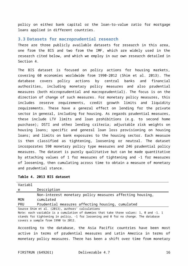
The BIS dataset is focused on policy actions for housing markets, covering 60 economies worldwide from 1990-2012 (Shim et al. 2013). The database covers policy actions by central banks and financial authorities, including monetary policy measures and also prudential measures (both microprudential and macroprudential). The focus is on the direction of change of such measures. For monetary policy measures, this includes reserve requirements, credit growth limits and liquidity requirements. These have a general effect on lending for the private sector in general, including for housing. As regards prudential measures, these include LTV limits and loan prohibitions (e.g. to second home purchase); DSTI and other lending criteria; adjustable risk weights on housing loans; specific and general loan loss provisioning on housing loans; and limits on bank exposures to the housing sector. Each measure is then classified as tightening, loosening or neutral. The dataset incorporates 590 monetary policy type measures and 246 prudential policy measures. The dataset is purely qualitative but can be made quantitative by attaching values of 1 for measures of tightening and -1 for measures of loosening, then cumulating across time to obtain a measure of monetary and prudential stance.

Table 4. 2013 BIS dataset

Variable DescriptionMON Non-interest monetary policy measures affecting housing, cumulatedPRU Prudential measures affecting housing, cumulatedSource Shim et al. (2013), authors’ calculationsNote: each variable is a cumulation of dummies that take three values: 1, 0 and -1. 1 stands for tightening in policy, -1 for loosening and 0 for no change. The database covers a sample from 1990 to 2012.

According to the database, the Asia Pacific countries have been most active in terms of prudential measures and Latin America in terms of monetary policy measures. There has been a shift over time from monetary to prudential measures as countries focused on macroprudential policy after the crisis, having earlier adjusted monetary policy towards inflation targeting.

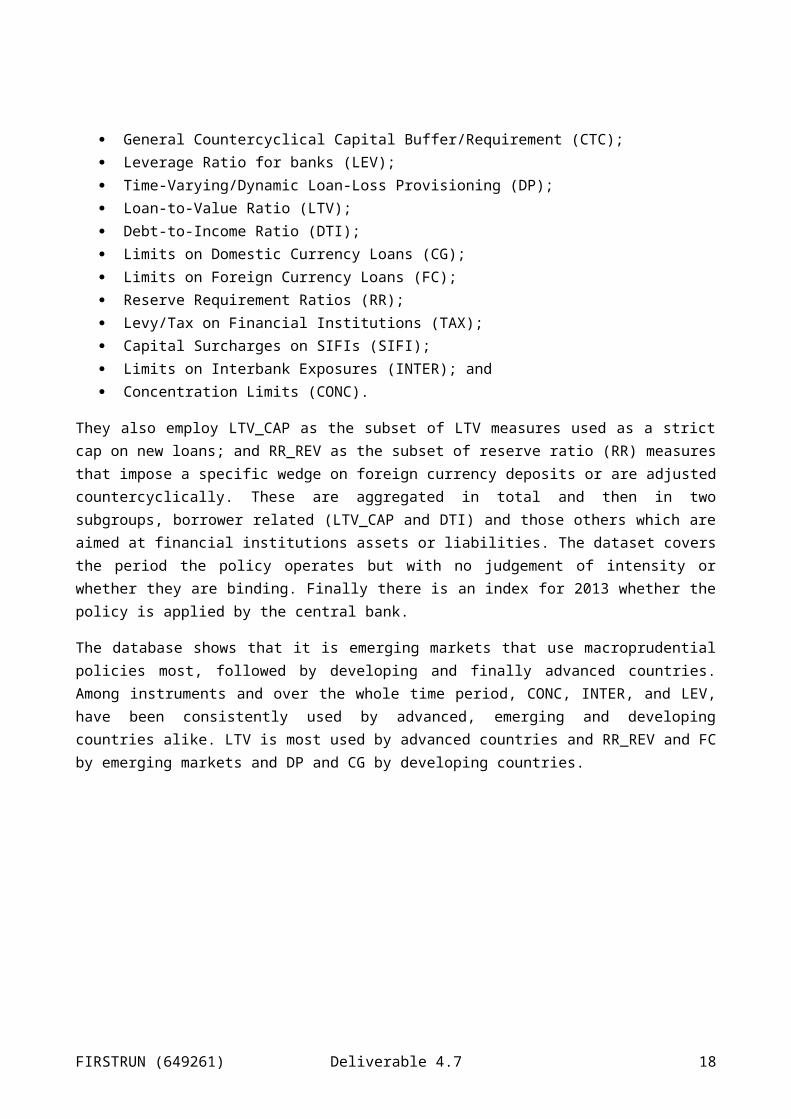
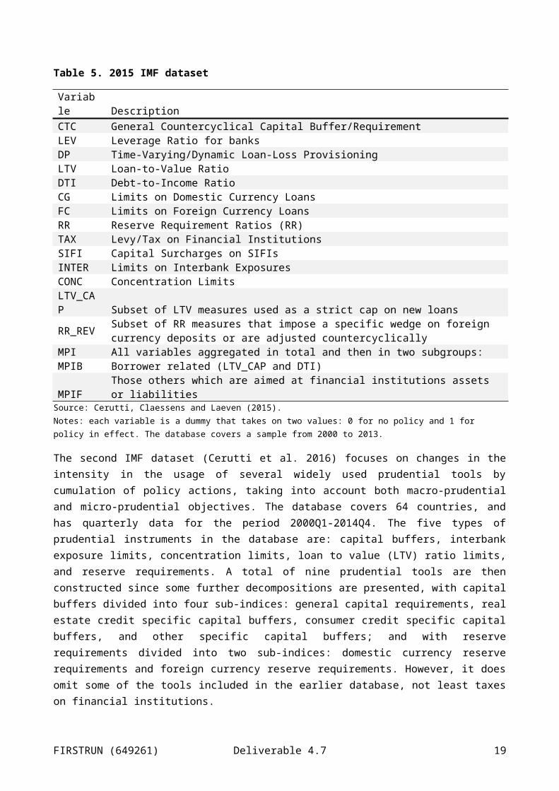
The first IMF dataset is set out in Cerutti, Claessens and Laeven (2015). It covers 119 economies over 2000-2013. It draws on the IMFs Global Macroprudential Policy Instruments (GMPI) survey. There are 12 instruments in the publicly available dataset, as follows:


General Countercyclical Capital Buffer/Requirement (CTC); Leverage Ratio for banks (LEV); Time-Varying/Dynamic Loan-Loss Provisioning (DP); Loan-to-Value Ratio (LTV); Debt-to-Income Ratio (DTI); Limits on Domestic Currency Loans (CG); Limits on Foreign Currency Loans (FC); Reserve Requirement Ratios (RR); Levy/Tax on Financial Institutions (TAX); Capital Surcharges on SIFIs (SIFI); Limits on Interbank Exposures (INTER); and Concentration Limits (CONC).

They also employ LTV_CAP as the subset of LTV measures used as a strict cap on new loans; and RR_REV as the subset of reserve ratio (RR) measures that impose a specific wedge on foreign currency deposits or are adjusted countercyclically. These are aggregated in total and then in two subgroups, borrower related (LTV_CAP and DTI) and those others which are aimed at financial institutions assets or liabilities. The dataset covers the period the policy operates but with no judgement of intensity or whether they are binding. Finally there is an index for 2013 whether the policy is applied by the central bank.

The database shows that it is emerging markets that use macroprudential policies most, followed by developing and finally advanced countries. Among instruments and over the whole time period, CONC, INTER, and LEV, have been consistently used by advanced, emerging and developing countries alike. LTV is most used by advanced countries and RR_REV and FC by emerging markets and DP and CG by developing countries.


Table 5. 2015 IMF dataset

Variable DescriptionCTC General Countercyclical Capital Buffer/RequirementLEV Leverage Ratio for banksDP Time-Varying/Dynamic Loan-Loss ProvisioningLTV Loan-to-Value RatioDTI Debt-to-Income RatioCG Limits on Domestic Currency LoansFC Limits on Foreign Currency LoansRR Reserve Requirement Ratios (RR)TAX Levy/Tax on Financial InstitutionsSIFI Capital Surcharges on SIFIsINTER Limits on Interbank ExposuresCONC Concentration LimitsLTV_CAP Subset of LTV measures used as a strict cap on new loans

RR_REV Subset of RR measures that impose a specific wedge on foreign currency deposits or are adjusted countercyclically

MPI All variables aggregated in total and then in two subgroups:MPIB Borrower related (LTV_CAP and DTI)MPIF Those others which are aimed at financial institutions assets or liabilities

Source: Cerutti, Claessens and Laeven (2015).Notes: each variable is a dummy that takes on two values: 0 for no policy and 1 for policy in effect. The database covers a sample from 2000 to 2013.

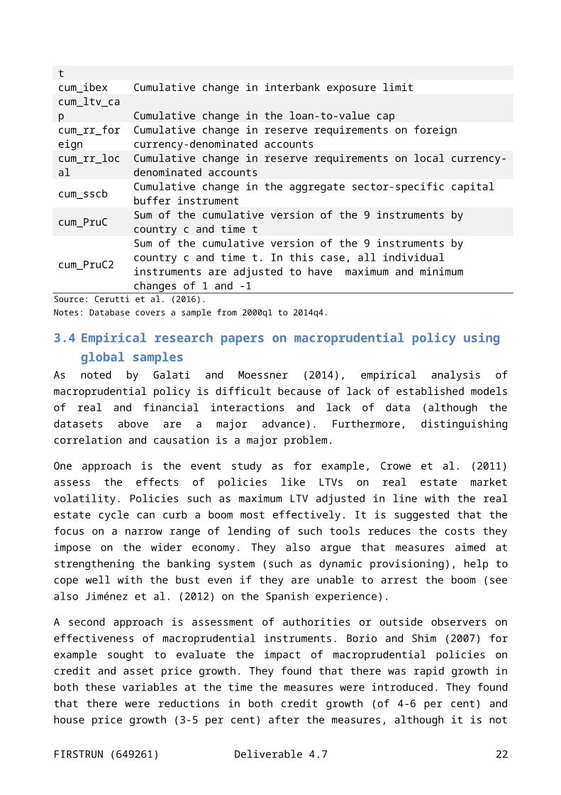
The second IMF dataset (Cerutti et al. 2016) focuses on changes in the intensity in the usage of several widely used prudential tools by cumulation of policy actions, taking into account both macro-prudential and micro-prudential objectives. The database covers 64 countries, and has quarterly data for the period 2000Q1-2014Q4. The five types of prudential instruments in the database are: capital buffers, interbank exposure limits, concentration limits, loan to value (LTV) ratio limits, and reserve requirements. A total of nine prudential tools are then constructed since some further decompositions are presented, with capital buffers divided into four sub-indices: general capital requirements, real estate credit specific capital buffers, consumer credit specific capital buffers, and other specific capital buffers; and with reserve requirements divided into two sub-indices: domestic currency reserve requirements and foreign currency reserve requirements. However, it does omit some of the tools included in the earlier database, not least taxes on financial institutions.


Table 6. 2016 IMF database

Variable DescriptionChanges in prudential instruments

sscb_res Change in sector specific capital buffer: Real estate credit. Requires banks to finance a larger fraction of these exposures with capital

sscb_cons Change in sector specific capital buffer: Consumer credit Requires banks to finance a larger fraction of these exposures with capital

sscb_oth Change in sector specific capital buffer: Other sectors. Requires banks to finance a larger fraction of these exposures with capital

cap_req Change in capital requirements. Implementation of Basel capital agreementsConcrat Change in concentration limit. Limits banks' exposures to specific borrowers or sectorsIbex Change in interbank exposure limit. Limits banks exposures to other banksltv_cap Change in the loan-to-value ratio cap. Limits on loans to residential borrowersrr_foreign Change in reserve requirements on foreign currency-denominated accountsrr_local Change in reserve requirements on local currency-denominated accountsAggregate indexes

Sscb Sum of changes in sector-specific capital buffers across the residential, consumer, and other sectors

PruC Country index by time t and country c, equal to 1 if the sum of the 9 instruments is >=1 and -1 if the sum of the instruments is <=-1, 0 otherwise

PruC2Country index by time t and country c, equal to 1 if the sum of the 9 instruments is >=1 and -1 if the sum of the instruments is <=-1, 0 otherwise. In this case, all individual instruments are adjusted to have maximum and minimum changes of 1 and -1

Cumulative indexes (relative to 2001q1)cum_sscb_res Cumulative change in sector specific capital buffer: Real estate creditcum_sscb_cons Cumulative change in sector specific capital buffer: Consumer credit

cum_sscb_oth Cumulative change in sector specific capital buffer: Other sectorscum_cap_req Cumulative change in capital requirementscum_concrat Cumulative change in concentration limitcum_ibex Cumulative change in interbank exposure limitcum_ltv_cap Cumulative change in the loan-to-value capcum_rr_foreign Cumulative change in reserve requirements on foreign currency-denominated accounts

cum_rr_local Cumulative change in reserve requirements on local currency-denominated accountscum_sscb Cumulative change in the aggregate sector-specific capital buffer instrumentcum_PruC Sum of the cumulative version of the 9 instruments by country c and time t

cum_PruC2Sum of the cumulative version of the 9 instruments by country c and time t. In this case, all individual instruments are adjusted to have maximum and minimum changes of 1 and -1

Source: Cerutti et al. (2016).Notes: Database covers a sample from 2000q1 to 2014q4.

3.4 Empirical research papers on macroprudential policy using global samplesAs noted by Galati and Moessner (2014), empirical analysis of macroprudential policy is difficult because of lack of established models of real and financial interactions and lack of data (although the datasets above are a major advance). Furthermore, distinguishing correlation and causation is a major problem.


One approach is the event study as for example, Crowe et al. (2011) assess the effects of policies like LTVs on real estate market volatility. Policies such as maximum LTV adjusted in line with the real estate cycle can curb a boom most effectively. It is suggested that the focus on a narrow range of lending of such tools reduces the costs they impose on the wider economy. They also argue that measures aimed at strengthening the banking system (such as dynamic provisioning), help to cope well with the bust even if they are unable to arrest the boom (see also Jiménez et al. (2012) on the Spanish experience).

A second approach is assessment of authorities or outside observers on effectiveness of macroprudential instruments. Borio and Shim (2007) for example sought to evaluate the impact of macroprudential policies on credit and asset price growth. They found that there was rapid growth in both these variables at the time the measures were introduced. They found that there were reductions in both credit growth (of 4-6 per cent) and house price growth (3-5 per cent) after the measures, although it is not always easy to divide the impact of such measures from that of monetary policy or economic growth and to assess what would have happened in the absence of such policies.

A third approach is of reduced form regressions, often using panel data. Here the weaknesses are that such regressions may not capture well the interaction of policy, real and financial sectors; there is little experience of macroprudential policy to assess the effect and transmission mechanism; and there is again a difficulty in isolating effects from those of monetary policy.

In an early study, Wong et al. (2011) look into the effectiveness of LTV limits in a panel of 13 countries over 1991-2010. They find that economies with LTV policy are estimated to have a lower sensitivity of mortgage delinquency ratios to property prices than those without LTV policy, taking into account other determinants of default (property prices, GDP growth, mortgage debt/GDP and interest rates), On the other hand, their model can be criticised as not being empirically robust, notably due to omitted variation in regulations.

Kuttner and Shim (2013) assess the effectiveness of nine non-interest rate policy tools, including macro-prudential measures, in stabilizing housing market prices and related lending in 57 countries over 1980-2011. They use panel regressions, with controls for the short rate and the growth in real GNI per capita. Housing credit growth is slower significantly by adjustments in the maximum debt-service-to-income (DSTI) ratio, the maximum LTV, limits on banks’ exposure to the housing sector and housing-related taxes. However, when using mean group and panel event study methods, only the DSTI ratio limit has a significant effect on housing credit growth. Furthermore, only a change in housing-related taxes significantly affects house price inflation.

Vandenbussche, Vogel, and Detragiache (2012) assess the relation between macro-prudential policies and house price inflation in Central, Eastern, and South-eastern European countries, using panel data techniques. Capital ratio requirements and non-standard liquidity measures (marginal reserve ratio on foreign funding or linked to credit growth) reduce house price inflation, according to their results.

Akinci and Olmstead-Rumsey (2015) construct an index of domestic macroprudential policies in 57 advanced and emerging economies covering 2000-2013. Effectiveness of policies in curbing bank credit and house prices is assessed using a dynamic panel data model where control variables include real GDP growth, change in nominal monetary policy rates and the VIX, a measure of the implied volatility of S&P 500 index options. Findings of the paper are that usage has become more active since the global financial crisis, in both advanced countries and EMEs; the main target is the housing market, and they are often related to bank reserve requirements, capital controls and monetary policy. Macroprudential tightening is


associated with lower bank credit growth, housing credit growth, and house price inflation and targeted policies are more effective. In EMEs capital inflow restrictions targeting the banking sector are also associated with lower credit growth, although portfolio flow restrictions are not. Without the measures, credit and asset price growth would have been much greater.

Cerutti et al. (2015) use a 2013 IMF survey (see Section 3.3) of annual macroprudential measures in 119 countries, with a panel GMM regression for macroprudential indicators with independent variables including GDP growth, the policy rate level and banking crises and country fixed effects as well as the macroprudential variables. An index summing all types of policy is correlated with lower credit growth, especially in EMEs. Borrower based policies like LTV and DSTI limits, as well as financial institutions based policies like limits on leverage and dynamic provisioning are shown to be particularly effective in reducing growth in real credit and house prices. Policies work best in the upturn but are less effective in a bust period. Macroprudential policy is weaker in more open and financially deeper economies, suggesting there is evasion cross border or in shadow banking. Countries with more cross border borrowing use macroprudential policies more.

Bruno, Shim and Shin (2015) provide a comparative assessment of the effectiveness of macro-prudential policies in 12 Asia-Pacific economies, using databases of both domestic macroprudential policies and capital flow management (CFM) policies over 2004-13, with 152 CFM measures and 177 domestic macroprudential measures. Estimation is by dynamic GMM to allow for endogeneity. They find that banking sector CFM polices and bond market CFM policies are effective in slowing down banking inflows and bond inflows, respectively and also there are spillover effects of these policies on the “other” type of inflows. Macroprudential policies tend to be introduced along with monetary tightening, and are most successful when they complement monetary policy by reinforcing monetary tightening.

Zhang and Zoli (2014) look at macroprudential and capital flow measures in 13 Asian and 33 other economies since 2000. Measures did help to limit growth in house prices, credit, equity prices and bank leverage with LTV, tax and foreign currency linked measures being most effective.

Lim et al. (2011) again using panel approaches assess links between macro-prudential policies, credit and leverage. They show some policies are effective in reducing the procyclicality of credit and leverage, notably tools such as LTV and DTI caps, ceilings on credit growth, reserve requirements, and dynamic provisioning rules.

Dell'Ariccia et al. (2012) assess the use of macro-prudential policies in diminishing credit booms and busts, both in terms of risk of a boom and its adverse effect on the economy. They find a reduction in the probability of a bad boom from such policies, in particular for those that culminate in a financial crisis, although they do not much affect the probability of adverse economic consequences. On balance, it is suggested that macro-prudential policies can reduce the risk of a bust, as well as adverse effect on the rest of the economy of financial system difficulties.

IMF (2013) assesses how changes in macroprudential policies affect financial vulnerabilities (credit growth, house prices, and portfolio capital inflows) as well as the impact on the real economy (output growth and the share of residential investment), and whether the effects of policies are more effective in the upturn or downturn. Their findings are that both time-varying capital requirements and reserve requirements affect credit growth; LTV limits and capital requirements have sizeable effects on house price rises, and that reserve requirements reduce portfolio inflows in emerging markets whose exchange rate regime is flexible.


However, only limits on LTV impact output growth, with the suggestion that this works through a reduction in investment in buildings and dwellings.

Macro stress tests can be used to assess responses of the financial system to large shocks see Drehmann (2009). For the most part, however, such studies do not allow for the potential large impact of small shocks, and omit feedback from the financial system to the macro economy (Borio and Drehmann 2009). However, Aikman et al. (2009) in their Risk Assessment Model for Systemic Institutions capture feedback effects from liquidity risk and procyclicality. Hence regulatory changes such as capital tightening can affect systemic risks. Bank of Canada work (Gauthier et al. 2012) looks at interbank spillover effects across major Canadian banks, entailing solvency, market and funding liquidity risks.

Counterfactual analysis seeks to assess what would have happened if macroprudential; policies had been applied to past events. Antipa et al. (2010) use a DSGE model of the US with a modified Taylor rule where the short rate responds to credit growth as well as inflation and authorities can influence the short term credit spread. Such a policy could have mitigated the last credit cycle and the succeeding recession. Catte et al. (2010) use the National Institute Global Econometric Model (NiGEM) for the US over 2002-7 and assume a policy was feasible that would influence spreads on mortgages4. This would again have mitigated the housing cycle. Barrell et al. (2010b) use a well-founded logit estimate of the determinants of banking crises in OECD countries (based on Barrell et al. (2010a) and were able to provide estimates of the degree of macroprudential regulatory tightening needed to reduce crisis probabilities in the subprime crisis and over earlier non-crisis periods to acceptable levels, as well as providing a useful tool for macroprudential surveillance able to predict crises sensitively without changes in specification over 1998-2008. They show that an international consensus on regulatory changes will generate “winners” and “losers” in terms of capital and liquidity adjustments, and that raising capital and liquidity standards by 3.7 percentage points across the board will reduce the annual average probability of a financial crisis to around 1 per cent. In Barrell et al. (2009) assessment is also made of costs as opposed to benefits of since higher capital and liquidity requirements induce banks to raise lending margins, hence adversely affecting the user cost of capital, investment and the capital stock.

Barrell et al. (2010b) also looked at how house prices should impact on macroprudential regulation generally. Against the background of their logit model predicting banking crises cited above, as well as arguments that credit growth should guide countercyclical provisioning, they suggest that the appropriate adjustment for procyclicality requires the country to calculate the trade-off between house prices, current account balances and regulatory variables over time. Since there is nonlinearity in a logit equation, there is not a simple rule that can be derived. Undertaking a scenario with house prices 5 percentage points higher, they showed that the regulatory adjustment is greater, as would be expected, with higher lagged house price growth, but the relationship is not one-to-one – it depends also on the other regulatory and non-regulatory variables in the model. A given growth rate of house prices is more threatening to financial stability when there is also low capital and liquidity as well as a current account deficit.

Davis, Fic and Karim (2011) again run NiGEM simulations for the Swedish economy following estimation of a house price equation for that country. Results suggest that macroprudential policies can have a distinctive impact on the economy, focused on the housing market, which could helpfully complement monetary policy at most points in the cycle. A generalised rise in capital adequacy is shown to have a quite marked impact in GDP, mainly via investment rather than consumption. However, a more focused capital adequacy

4 https://nimodel.niesr.ac.uk/


rise for mortgage lending only or an LTV policy appear to have scope to reduce house prices with less effect on the rest of the economy than other options, although it may of course be more subject than capital adequacy based policies to disintermediation. Capital adequacy for mortgage lending affects GDP more than the LTV policy since it impacts more on personal income and hence consumption. Monetary policy does of course also affect housing market variables but also has a greater effect on the wider economy, as do generalised rises in capital ratios affecting all lending.

Whatever the context, it is clear that the correct modelling of house prices and credit is crucial and is likely to receive increasing attention in the wake of the sub-prime crisis and policy developments; it is this issue we turn to in the next section. The determinants of house prices and credit may either capture directly the impact of policy, or identifies key driving variables which would otherwise bias the results of estimation – and which may in any case be indirectly affected by policy in a macroeconomic context.

Finally, micro data has been rather little used in the debate to date. Using Korean survey data, Igan and Kang (2012) find beneficial effects of LTV and DTI limits on mortgage credit growth in Korea. Gauthier et al. (2012) find that macroprudential capital requirements reduce probabilities of crises and of individual bank failures in Canada by around 25 per cent. In the UK over the period 1998-2007, Aiyar et al. (2013) find that bank-specific higher capital adequacy requirements dampened lending by individual banks (whereas tighter monetary policy did not affect the supply of lending). On the other hand, bank capital requirements were ineffective due to increased lending from the branches of foreign banks.

Claessens et al. (2014) seek to analyse the impact of macroprudential policies in limiting vulnerability of individual banks’ balance sheets. They assess 48 countries, 25 advanced and 23 EMEs, with 2820 banks and 18000 observations. They group the macro-prudential policies according to whether they are aimed at borrowers (caps on debt-to-income (DTI) and loan-to-value (LTV) ratios), banks’ assets or liabilities (limits on credit growth (CG), foreign currency credit growth (FC) and reserve requirements (RR)), policies that encourage counter-cyclical buffers (counter-cyclical capital (CTC), dynamic provisioning (DP) and profits distribution restrictions (PRD)) and a final group of miscellaneous policies (which have some overlap with the first three groups). They perform panel, GMM regressions relating these policies to changes in individual banks’ assets. They find that policies aimed at borrowers are effective in (indirectly) reducing the build-up of banking system vulnerabilities. Measures aimed at banks’ assets and liabilities are very effective, but counter-cyclical buffers as a group show less promise. The category “other” is also very effective. In upturns, all the measures except buffers reduce bank asset growth. Whereas borrower based measures are also relatively less effective, they do appear to limit "credit crunches" in contractionary periods. Between advanced countries and EMEs the main difference is the greater effectiveness of borrower based measures in advanced countries. A package of measures appears to work best in EMEs, perhaps as their financial systems are less liberalised. But no policy seems to be effective in counteracting a "credit crunch" in the downturn.

Looking briefly at national as opposed to global studies, Igan and Kang (2012) find LTV and DTI limits to moderate mortgage credit growth in Korea. And macroprudential policies targeted at real estate borrowing appear to reduce real estate cycles in Hong Kong (Wong and Hui 2010).

The existing empirical studies are summarised in Table 25 in appendix B.


4 Modelling the impact of macroprudential policiesOur starting point is that many studies cited above have sought to cover global samples, but at a cost of having a rather limited set of control variables for macroprudential. We are focusing here on OECD countries, notably in Europe, and accordingly can use a better and more precise set of controls. Our chosen target variables, in line with much of the literature, are real house prices and real household sector credit. The macroprudential instrument datasets used are the first and second IMF dataset and summary measures derived from the BIS dataset as outlined in Section 2.3.

Typical estimates for determination of house prices are in error correction format. There is first a cointegrating levels equation which forms an inverted demand function for housing but also includes a supply effect such as the stock of housing which determines the long-run price of housing (Meen (2002), Barrell and Kirby (2004, 2011) Adams and Fuss (2012), Loungini and Igan (2012), Muellbauer and Murphy (2008), Capozza et al. (2002)). This first stage equation constitutes the relationship that drives the long-run properties of the dependent variable and can be written as the following regression equation:

Y tc=X t

c βc+εtc

Where Y is a Tx1 vector containing the dependent variable in log levels, t denotes the time period, c is a country index, X is a TxN matrix of N regressors in log levels including a constant, β is an Nx1 vector of coefficients and ε is the residual term.

This first stage equation is incorporated into an expanded equation that recognises that actual house prices deviate from their fundamental values in the short-run and typically includes a set of controls in first differences to allow for these dynamics. For the error correction equation to be meaningful there has to be a cointegrating relationship between the long-run variables (the first stage regression step) and the elements capturing the short-term dynamics must be stationary. This set up allows the examination of factors that drive house price dynamics. The second stage can be written as:

∆Y tc=α c+λc (Y tc−X tc βc)+∆Z tc+ϵ tc

Where α denotes a constant, Z is a set of regressors aimed at capturing short-term deviations of the dependent variable from the long-run relationship and ϵ is the error term. The two stages may be combined, as in our work shown below, in a single stage error correction estimation. A similar approach is adopted for credit.

Variables used are as follows: log real house prices (LRPH), log real personal disposable income (LRPDI), the real long rate (LRR), log real household liabilities (LRLIABS), log real gross financial wealth (LRGW), unemployment rate (U) and log real housing capital stock (LRKH). The Im-Pesaran-Shin panel unit root tests for the main variables (not illustrated) show most variables, being trended, are I(1) thus justifying an error correction model based approach to estimation. Changes in real house prices were regressed on contemporaneous changes in explanatory variables, and lagged dependent and explanatory variables (both in levels) as well. This error-correction specification is able to deal with non-stationarity in the data, and at the same time distinguishing short- and long-run influences, and differences between cycles. The significance of the coefficients for lagged non-stationary variables (in levels) and their magnitude reveal the long-term relationship among those variables.


Following the bulk of the literature, our panel modelling started from the panel error-correction approach of Davis, Fic and Karim (2011), also employed in Armstrong and Davis (2014), with an extended house price equation including real house prices, real personal disposable income and the long term real interest rate (proxying the user cost) as well as the rate of unemployment, real gross financial wealth (as a portfolio balance effect), housing stock (lag only), household credit (lag only) and dummies for financial crises. We estimated corresponding equations for mortgage credit, viewing this as a further portfolio balance equation, albeit closely linked to housing.

We used data from 2000Q1-2015Q4 with quarterly observations for up to 18 advanced OECD countries from the NiGEM database, the short estimation period being necessitated by the short period covered by the macroprudential databases5. The countries are Australia, Belgium, Canada, Denmark, Finland, France, Germany, Greece, Ireland, Italy, Japan, Netherlands, Austria, Portugal, Sweden, Spain, the UK and the US.

We undertake panel regression that treats all countries as equally important, while the country fixed effects take account of heterogeneity, and we impose cross section weights. In each case we eliminated insignificant variables. The initial estimates are tabulated in Table 8 below. To confirm the existence of the long-term relationship, we also implement the panel cointegration test proposed by Kao (1999) among those variables with significant lagged level terms in a simple levels equation (i.e. the first step of an Engle and Granger (1987) two-step estimation). As shown in the table, the test rejects comfortably the null of no cointegration for the panel regressions on real household credit growth, while it barely rejects the null at the 10 per cent significance threshold for real house price growth.

To address the weak cointegrating relationship in real house price growth we estimate country by country error correction equations in a seemingly unrelated regression (SUR) framework. For the sake of completeness we perform the same robustness check for real household credit growth. The results are reported and discussed in Section 5.

It can be seen in Table 7 that for house prices the dynamic specification includes real personal disposable income, real long rates, unemployment and real household wealth and also the lagged difference of credit. It also includes a lagged house price variable as an “accelerator”. In the long run, the specification includes the levels of RPDI, long real rates and the housing capital stock, all with correct signs. As regards credit growth, the dynamic terms are real personal disposable income and real wealth while the long term effects arise from house prices, the stock of housing, and the level of unemployment. The crisis variable is significant for both house prices and credit. The Kao panel cointegration test is passed at the 99 per cent level for the credit equation but only 90 per cent level for the house price equation.

5 https://nimodel.niesr.ac.uk/


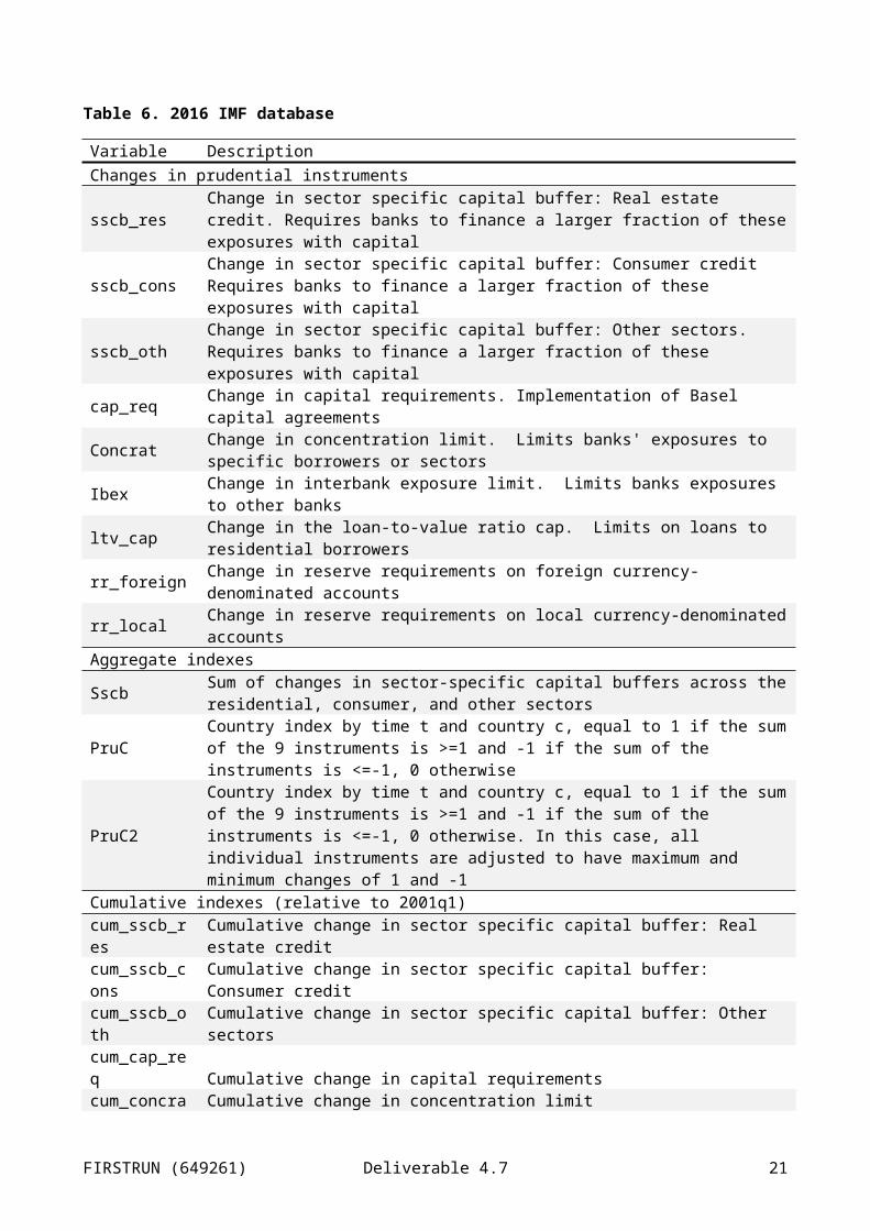
Table 7. Baseline equations (2000Q1-2015Q4)

Variable Real house price growth (DLRPH)

Real household credit growth (DLRLIABS)

C 0.185*** (2.9)

0.373*** (6.0)

DLRPDI 0.129*** (4.8)

0.108*** (4.2)

DLRR -0.0033** (2.4)

DLRPH(-1) 0.397*** (14.6)

DLRLIABS (-1) 0.097*** (3.4)

DLRLIABS (-2) 0.065*** (2.7)

DLRLIABS (-3) 0.082*** (3.5)

LRLIABS (-1) -0.019*** (6.1)

LRPH(-1) -0.0165*** (5.3)

0.025*** (6.1)

LRPDI(-1) 0.026*** (3.2)

LRR(-1) -0.0014*** (2.8)

LKH(-1) -0.035*** (4.8)

-0.021*** (3.5)

DU -0.0039*** (3.5)

U(-1) -0.0014*** (6.8)

DLRGW 0.059*** (4.2)

0.087*** (6.6)

CRISES -0.0029*** (2.7)

-0.0042*** (4.7)

R2 0.56 0.53 SE 0.015 0.012 OBS 1081 1081

KAO -1.4* (0.08)

-4.3*** (0.0)

COUNTRIES 18 18

Notes: lrph is the log real house price, lrr is the long term real rate, lrpdi is the log real personal disposable income, lrliabs is the log real household credit, lrgw is the log gross wealth, lkh is the log of the housing capital stock, u is the unemployment rate, and crises is a dummy for financial crisis taking a value of 1 when a financial crisis has occurred and 0 otherwise. Whenever a “d” appears in front of a variable it denotes the variable is in first differences. *** denotes that the coefficient is significant at the 1 per cent significance threshold, a ** denotes significance at the 5 per cent threshold and a * at the 1 per cent threshold. T-stats are reported in parenthesis below each estimated coefficient.

We tested the macroprudential variables in this framework one by one, (for variable definitions see Tables 4-5). We see in Table 8 that house prices are affected significantly by the summary variables MPI (which


aggregates all macroprudential variables) and MPIB (aggregating macroprudential variables affecting the borrower), as well as LTV, DTI, TAX (taxes on financial intermediaries) and LTV_CAP (the subset of LTV measures used as a strict cap on new loans). Credit growth is affected by MPI, MPIF (aggregating macroprudential policies which are aimed at financial institutions assets or liabilities), DTI (with the wrong sign), TAX, and INTER (limits on interbank lending).

The summary BIS variable PRU (general prudential measures affecting housing) is significant for house prices over the period since 1990, as is MON (non interest monetary measures affecting housing) for credit over the same period.

Table 8. Results with the first IMF and BIS datasets using baseline



MPI -0.002** (2.4)

-0.0016** (2.3)

MPIB -0.0023** (2.3)

0.0018 (1.5)

MPIF -0.0013 (0.9)

-0.0031*** (3.8)

LTV -0.0023* (1.7)

-0.0023 (1.3)

DTI -0.004** (2.0)

0.0043* (1.8)

FC 0.007 (0.7)

-0.0036 (1.0)

TAX -0.0039* (1.7)

-0.0074*** (4.7)

INTER 0.0006 (0.2)

-0.0045*** (2.7)

CONC -0.004 (0.6)

0.0026 (0.6)

LTV_CAP -0.0047** (2.4)

0.0024 (1.1)

MON 0.0015 (0.6)

0.0021 (0.9)

PRU -0.00010 (0.3)

0.00067 (0.8)

MON (estimated from 1990) 0.0007 (0.4)

-0.0088*** (2.5)

PRU (estimated from 1990) -0.0012* (1.7)

-0.00073 (0.9)

Notes: for variables definitions see tables 4 and 5. T-stats are reported in parenthesis below each estimated coefficient.

For European countries there are similar albeit somewhat weaker results from this specification. LTV however is not effective in house prices (although LTV_CAP remains significant), while MON is not significant for lending.


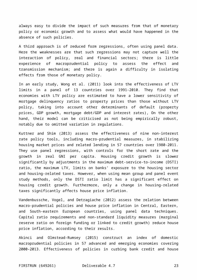
Table 9. Results with the first IMF and BIS datasets using baseline equations (Europe only)



MPI -0.0025* (1.9)

-0.0028*** (3.6)

MPIB -0.0052* (1.9)

-0.0016 (0.6)

MPIF -0.0017 (1.1)

-0.0032*** (3.7)

LTV -0.0016 (0.9)

-0.0057*** (2.8)

FC 0.0074 (0.8)

-0.0029 (0.9)

TAX -0.0049** (2.0)

-0.0072*** (4.2)

INTER 0.00008 (0.1)

-0.0046*** (2.6)

LTV_CAP -0.0074** (2.1)

-0.0026 (0.7)

MON 0.0012 (0.5)

0.0014 (0.6)

PRU -0.0008 (0.8)

0.00064 (0.6)

MON (estimated from 1990) 0.0098** (2.2)

-0.00066 (1.4)

PRU (estimated from 1990) -0.0019* (1.9)

0.00052 (0.5)


We then went on to assess how results would differ using a more simple specification that is typical of the literature. So for example in Akinci and Olmstead-Rumsey (2015), effectiveness of policies in curbing bank credit and house prices is assessed using a dynamic panel data model where control variables besides a lagged dependent variable include real GDP growth, change in nominal monetary policy rates (R3M) and the VIX volatility measure based on US share prices. This specification has the advantage of enabling developing and emerging market countries that have relatively sparse macroeconomic data to be included in the regression. In contrast our extended specification could not readily cover a wider range of countries. The simpler specification for the same 18 countries is depicted in Table 10 below. Note this is not a direct comparison with Akinci and Olmstead-Rumsey (2015) since we are using EGLS rather than GMM as in their work and also we are using different datasets of macroprudential variables. Rather, it is an exercise in assessing the impact of using a richer range of independent variables in tests of macroprudential policies in OECD countries.


Table 10. Simpler specification typical in the literature (2000Q1-2015Q4)



C 0.008*** (2.7)

0. 006** (2.1)

DLGDP(-1) 0.121*** (2.7)

0.108** (2.2)

DLGDP(-2) 0.045 (1.0)

0.139*** (2.9)

LVIX -0.0024** (2.5)

-0.0005 (0.5)

DR3M (-1) -0.0006 (0.6)

-0.0015 (1.5)

DEPENDENT (-1) 0.562*** (22.4)

0.392*** (14.6)

R2 0.454 0.353 SE 0.016 0.015 OBS 1145 1135 COUNTRIES 18 18 Notes: T-stats are reported in parenthesis below each estimated coefficient.

From Table 11 it can be seen that with this specification a significant number of macroprudential tools are shown to be effective across these major OECD countries, including MPI and MPIB for house prices and credit growth, and MPIF for credit. Also, LTV, DTI, TAX and LTV_CAP are shown to be effective for both. FC (Limits on Foreign Currency Loans) and INTER (interbank lending limits) are effective for credit also. Of the BIS variables, PRU is shown to be effective for both also, as is MON if estimated back to 1990.


Table 11. Results using simpler specification



MPI -0.0019*** (2.9)

-0.0023*** (3.7)

MPIB -0.002*** (2.9)

-0.002** (2.1)

MPIF -0.0018 (1.5)

-0.0027*** (3.2)

LTV -0.0049*** (4.2)

-0.0058*** (3.9)

DTI -0.0037** (2.3)

-0.0037* (1.9)

FC 0.0022 (0.2)

-0.0063* (1.8)

TAX -0.0042** (2.2)

-0.0048*** (3.2)

INTER -0.0004 (0.2)

-0.0035** (2.0)

CONC -0.0044 (0.7)

-0.0034 (0.7)

LTV_CAP -0.0039*** (2.7)

-0.004** (2.2)

MON 0.0033 (1.4)

0.0035 (1.3)

PRU -0.001* (1.9)_

-0.0018*** (2.6)

MON (estimated from 1990) -0.0006** (2.1)

-0.0002 (0.7)

PRU (estimated from 1990) -0.0006 (0.9)

-0.0009 (1.4)


For the EU only there are similar positive results in most cases (Table 12), albeit not for MPI or MPIB in the case of house prices, MPIB and PRU for credit or for DTI in both cases.


Table 12. Results using simpler specification (Europe only)



MPI -0.0017 (1.6)

-0.0027*** (3.4)

MPIB -0.0032 (1.2)

-0.0047 (1.6)

MPIF -0.0015 (1.2)

-0.0027*** (3.2)

LTV -0.0053*** (3.1)

-0.0078*** (3.8)

DTI -0.036 (0.5)

-0.008 (1.1)

FC 0.0026 (0.2)

-0.0063* (1.8)

TAX -0.004** (2.0)

-0.0048*** (3.2)

INTER -0.00027 (0.1)

-0.0036** (2.1)

LTV_CAP -0.0046 (1.3)

-0.0066* (1.6)

MON 0.003 (1.3)

0.0032 (1.2)

PRU -0.002* (1.8)

-0.0018 (1.4)

MON (from 1990) -0.00035 (1.0)

0.00045 (1.2)

PRU (from 1990) -0.0019 (2.0)

-0.0008 (0.7)


We went on to test the second IMF database on the extended and simple model (Table 13). We find as above that there are more significant variables with the simple than the extended model. That said, there are significant results in the extended model for cumulated concentration rules for house prices and for cumulated general prudential controls, capital requirements and interbank exposure limits as well as general prudential limits, non-cumulated capital requirements and interbank exposure limits for credit. There are also significant variables with the wrong sign in the case of reserve requirements bearing on local currencies6 and LTV limits.

For the simple model we find a great deal more significant variables for house prices such as cumulated interbank exposure limits, concentration limits, capital requirements, general prudential controls and real estate capital buffers as well as local reserve requirements with the wrong sign. For real credit, besides the above, we see an effect of real estate capital buffers as well as consumption and other buffers with the wrong sign.

6 The difficulty in getting “right signs” for reserve requirements may link to their dual role as an instrument of monetary policy and of macroprudential policy. See for example Izquerido et al. (2013) on related issues in Latin America.


Table 13. Results with second IMF database

Variables Extended specification Simpler specification House prices Real credit House prices Real credit

_SSCB_RES 0.0003 (0.1)

-0.0037 (0.8)

-0.0016 (0.3)

-0.0011 (0.2)

_SSCB_OTH 0.004 (0.2)

0.00167 (0.2)

0.0096 (0.5)

0.0062 (0.6)

_SSCB_CONS 0.0043 (0.2)

0.0016 (0.2)

0.0096 (0.5)

0.0062 (0.6)

_SSCB 0.0006 (0.1)

-0.0011 (0.4)

0.0024 (0.1)

0.0065 (0.2)

_RR_LOCAL -0.001 (0.4)

0.0073*** (3.1)

-0.0029 (1.1)

0.0064** (2.4)

_PRUC2 -0.0006 (0.4)

-0.002* (1.7)

-0.0013 (1.0)

-0.0041*** (3.1)

_PRUC -0.0006 (0.4)

-0.002* (1.7)

-0.0013 (1.0)

-0.0041*** (3.1)

_LTV_CAP 0.0039* (1.8)

0.0053** (2.4)

0.004* (1.8)

0.0045* (1.9)

_IBEX -0.00028 (0.1)

-0.0075*** (3.1)

-0.0028 (0.6)

-0.0076*** (3.0)

_CONCRAT -0.0047 (1.3)

0.0016 (0.4)

-0.026 (0.8)

-0.0042 (0.8)

_CAP_REQ -0.0004 (0.3)

-0.008*** (4.2)

-0.0012 (0.6)

-0.0097*** (4.8)

_CUM_SSCB_RES 0.0009 (0.4)

0.0001 (0.1)

-0.0058*** (3.2)

-0.011*** (6.4)

_CUM_SSCB_OTH -0.001 (0.2)

0.0024 (0.9)

0.0037 (0.8)

0.0068*** (2.6)

_CUM_SSCB_CONS -0.001 (0.2)

0.0024 (0.9)

0.0037 (0.8)

0.0068*** (2.6)

_CUM_SSCB 0.0003 (0.2)

0.0005 (0.6)

-0.0025* (1.8)

-0.0025** (2.3)

_CUM_RR_LOCAL 0.0021 (1.3)

0.0048*** (3.7)

0.0048*** (3.6)

0.0076*** (5.5)

_CUM_PRUC2 -0.0007* (1.7)

-0.0013*** (3.5)

-0.001*** (3.4)

-0.0017*** (5.1)

_CUM_PRUC -0.0007* (1.7)

-0.0013*** (3.5)

-0.001*** (3.4)

-0.0017*** (5.1)

_CUM_LTV_CAP 0.0011 (1.3)

0.0003 (0.3)

0.0049 (0.7)

0.00035 (0.4)

_CUM_IBEX -0.0009 (0.7)

-0.0031*** (3.3)

-0.0025** (2.0)

-0.0011 (1.5)

_CUM_CONCRAT -0.0019 ** (2.1)

-0.0045*** (3.4)

-0.0037*** (4.9)

-0.0072*** (5.4)

_CUM_CAP_REQ -0.0015* (1.9)

-0.003*** (3.9)

-0.0014** (2.4)

-0.0042*** (6.4)

Notes: For variable definitions see table 6. T-stats are reported in parenthesis below each estimated coefficient.


We estimated a simple panel vector error correction model with endogenous variables being log house prices, log credit, log RPDI and long real rates, one lag. Exogenous variables are dummies for crises and the macroprudential variables from the IMF and BIS databases, the latter introduced one at a time while the crisis effects are present for each estimate. As shown below, there are a number of significant effects for house prices, including the summary variables MPI and MPIF, as well as LTV and CONC (concentration limits) and (with positive signs) FC and MON (BIS variable for non-interest monetary policy measures affecting the housing market). For credit the positive results are more sparse, but include FC and TAX as significant restraints on credit growth, given the other included variables.

Table 14. Preliminary results with a panel VECM

Variable

Global Europe Real house price growth (DLRPH)


Real house price growth (DLRPH)


MPI -0.00076* (1.8)

-0.00038 (1.1)

0.0003 (0.6)

-0.0008* (1.6)

MPIB -0.0032*** (2.6)

-0.0001 (0.1)

-0.0034 (1.8)

0.00022 (0.1)

MPIF -0.0005 (1.0)

-0.0005 (1.3)

0.0012* (1.7)

-0.001* (1.8)

LTV -0.0034*** (2.7)

-0.0006 (0.6)

-0.0027 (1.6)

-0.0005 (0.4)

DTI -0.0068** (2.2)

-0.0024 (0.9)

-0.014 (1.6)

-0.0095 (1.3)

FC 0.0058 (1.5)

-0.0078** (2.3)

0.0052 (1.2)

-0.0072** (2.0)

TAX -0.0002 (0.1)

-0.0055*** (4.0)

-0.00017 (0.1)

-0.0056*** (3.7)

INTER 0.0003 (0.2)

-0.0007 (0.7)

0.002 (1.3)

-0.0017 (1.2)

CONC -0.0011 (1.0)

0.0005 (0.5)

0.0008 (0.6)

0.0004 (0.3)

LTV_CAP -0.0039** (2.3)

0.0007 (0.5)

-0.0029 (1.4)

0.0008 (0.5)

MON -0.0004 (1.4)

0.0004* (1.7)

0.00043 (1.6)

0.0011** (2.4)

PRU -0.0004 (0.6)

0.0007 (1.0)

0.00019 (0.2)

0.00032 (0.2)

MON (from 1990) 0.00036* (1.7)

0.0036 (1.0)

-0.0007** (2.1)

0.00054* (1.7)

PRU (from 1990) -0.00065 (1.0)

-0.0001 (0.1)

-0.00018 (1.2)

0.0018** (2.0)

Notes: For variable definitions see tables 4 and 5. T-stats are reported in parenthesis below each estimated coefficient.

In table 15 we show the results from adding the macroprudential variables that come from the second IMF database.


Table 15. Results with second IMF database

Variables Real house price growth (DLRPH)


_SSCB_RES 0.002 (0.3)

0.0008 (0.2)

_SSCB_OTH 0.003 (0.2)

0.008 (0.6)

_SSCB_CONS 0.003 (0.2)

0.008 (0.6)

_SSCB 0.0013 (0.3)

0.0015 (0.4)

_RR_LOCAL -0.0049 (1.4)

0.0078 (2.4)

_PRUC2 -0.0036** (2.0)

-0.0034** (2.1)

_PRUC -0.0036** (2.0)

-0.0034** (2.1)

_LTV_CAP -0.0009 (0.3)

0.005* (1.8)

_IBEX 0.0005 (0.1)

-0.01** (2.9)

_CONCRAT -0.001 (0.3)

0.0005 (0.1)

_CAP_REQ -0.0049* (1.7)

-0.012*** (4.9)

_CUM_SSCB_RES -0.0008 (0.6)

-0.003*** (2.6)

_CUM_SSCB_OTH -0.0001 (0.1)

0.0037 (1.3)

_CUM_SSCB_CONS -0.0001 (0.1)

0.0037 (1.3)

_CUM_SSCB -0.00043 (0.4)

-0.00094 (1.1)

_CUM_RR_LOCAL 0.00087 (1.0)

0.0025*** (3.4)

_CUM_PRUC2 0.00003 (0.1)

-0.0012*** (3.9)

_CUM_PRUC 0.00003 (0.1)

-0.0012*** (3.9)

_CUM_LTV_CAP 0.00007 (0.1)

0.004 (0.7)

_CUM_IBEX 0.0007 (1.2)

-0.0013** (2.3)

_CUM_CONCRAT 0.00005 (0.1)

-0.0015* (1.9)

_CUM_CAP_REQ -0.0017* (1.8)

-0.0065*** (8.0)

Notes: For variable definitions see tables 4 and 5. T-stats are reported in parenthesis below each estimated coefficient.

Finally in Table 16 we show results for European countries only with the second IMF database. These are comparable to those recorded above.


Table 16. Europe: results for macroprudential tools (second IMF database)

Variables Extended model Simple model VECM

House prices Real credit House prices Real credit House prices Real credit

_SSCB_RES 0.00046 (0.1)

-0.0039 (0.6)

-0.0034 (0.8)

-0.0047 (0.6)

0.0007 (1.0)

-0.0003 (0.1)

_SSCB 0.00046 (0.1)

-0.0039 (0.6)

-0.0034 (0.8)

-0.0047 (0.6)

0.0007 (1.0)

-0.0003 (0.1)

_RR_LOCAL -0.0008 0.9)

0.0074*** (3.2)

-0.004 (1.3)

-0.003* (1.9)

-0.0049 (1.3)

0.0082** (2.4)

_PRUC2 -0.029* (1.8)

-0.0013 (0.9)

-0.0046*** (2.8)

-0.003* (1.9)

-0.0062*** (2.8)

-0.002 (1.0)

_PRUC -0.029* (1.8)

-0.0013 (0.9)

-0.0046*** (2.8)

-0.003* (1.9)

-0.0062*** (2.8)

-0.002 (1.0)

_LTV_CAP 0.0018 (0.5)

0.0054* (1.9)

0.0026 (0.6)

0.007** (2.0)

-0.0053 (0.9)

0.0062* (1.8)

_IBEX -0.0033 (0.8)

-0.0051** (2.1)

-0.0066 (1.5)

-0.0065** (2.3)

-0.0084** (2.0)

-0.0087** (2.1)

_CONCRAT -0.004 (1.3)

0.0011 (1.3)

-0.004 (1.2)

-0.0047 (0.9)

-0.0018 (1.4)

0.00028 (0.1)

_CAP_REQ -0.0017 (0.7)

-0.007*** (3.4)

-0.0025 (1.0)

-0.008*** (3.2)

-0.0064* (1.8)

-0.012*** (3.6)

_CUM_SSCB_RES -0.0007 (0.3)

0.0005 (0.3)

-0.0065*** (3.3)

-0.015*** (7.4)

-0.0022 (1.4)

-0.0037*** (2.8)

_CUM_SSCB -0.0007 (0.3)

0.0005 (0.3)

-0.0065*** (3.3)

-0.015*** (7.4)

-0.0022 (1.4)

-0.0037*** (2.8)

_CUM_RR_LOCAL 0.0027 (1.6)

0.0041*** (3.0)

0.0048*** (3.4)

0.075*** (5.3)

0.0036*** (2.8)

0.0066*** (6.2)

_CUM_PRUC2 -0.00089* (1.9)

-0.001*** (2.9)

-0.0016*** (3.8)

-0.002*** (4.4)

-0.00001 (0.2)

-0.0013*** (3.5)

_CUM_PRUC -0.00089* (1.9)

-0.001*** (2.9)

-0.0016*** (3.8)

-0.002*** (4.4)

-0.00001 (0.2)

-0.0013*** (3.5)

_CUM_LTV_CAP 0.0012 (0.7)

0.0014 (1.0)

0.0037*** (2.6)

0.0045*** (3.1)

-0.00028 (0.3)

0.001 (1.5)

_CUM_IBEX -0.0015 (1.1)

-0.0003 (0.3)

-0.0019 (1.6)

-0.0013 (1.6)

-0.0016** (2.0)

-0.0004*** (4.7)

_CUM_CONCRAT -0.0025*** (2.6)

-0.004*** (3.2)

-0.0037*** (4.8)

-0.008*** (5.6)

-0.0005 (0.7)

-0.0015* (1.7)

_CUM_CAP_REQ -0.0007 (0.7)

-0.0034*** (3.5)

-0.002** (2.4)

-0.0049 (5.7)

-0.0025** (2.0)

-0.0078*** (7.4)

Notes: T-stats are reported in parenthesis below each estimated coefficient.

Tables 17 and 18 provide a summary of results from the Section. As can be seen, the extended estimates (with a wider range of appropriate variables) show less favourable results for macroprudential policies than the simple estimates more typical of the literature. The VECM, which also has quite a limited set of variables, is intermediate. That said, it is clear that some policies are shown as more effective than others in the 18 countries we study over 2000-2013. These include, in particular, taxes on financial institutions (TAX) and strict loan-to-value ratio limits (LTV_CAP). Limits on foreign currency lending (FC), debt-to-income ratio limits (DTI), limits on interbank exposures (INTER) and concentration limits (CONC) are also shown to be effective in some estimates. We cannot exclude that the use of these policies being quite limited and also affected by the financial crisis, further significant effects could emerge in the future.


Table 17. Summary table for macroprudential tools (first IMF and BIS databases)

Extended global

Extended Europe

Simple global

Simple Europe

VECM global

VECM Europe

Variable PH CR PH CR PH CR PH CR PH CR PH CR MPI -** -** -* -*** -*** -*** -*** -* -* MPIB -** -* -*** -** -* MPIF -*** -*** -*** -*** -* +* -* LTV -* -*** -*** -*** -*** -*** -** DTI -** +* -** -* FC -* -* -** -* -** TAX -* -*** -** -*** -** -*** -** -*** -*** -*** INTER -*** -** -** CONC -*** LTV_CAP -** -** -*** -** -* MON +** PRU -* -*** -* MON 90 -*** +** -** +** -** +* PRU 90 -* -* -** +* Notes: + denotes a positive relationship between the variables of interest, - denotes a negative relationship. Significance at the 1, 5 and 10 per cent thresholds are denoted by ***,** and * respectively.

The second IMF database highlights cumulated concentration rules (CUM_CONCRAT), general prudential controls (CUM_PRUC and PRUC2), implementation of Basel capital requirements (CUM_CAP_REQ) and interbank exposure limits (CUM_IBEX), whereas local currency reserve requirements on deposits (CUM_RR_LOCAL) appear to be often counterproductive. Capital buffers themselves (SSCB and SSCB_RES) are also supported by these estimates to some extent.


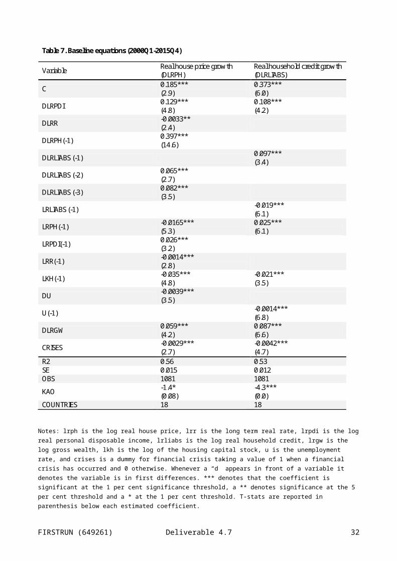
Table 18. Summary table for macroprudential variables (second IMF database)

Extended Global

Simple Global

VECM Global

Extended Europe

Simple Europe

VECM Europe

Variables PH CR PH CR PH CR PH CR PH CR PH CR _RR_LOCAL +*** +** +** +*** +** +** _RR_FOREIGN -*** _PRUC2 -* -*** -** -** -* -*** -*** -*** _PRUC -* -** -** -* -*** -*** -*** _LTV_CAP +* +** +* +* +* +* +* _IBEX -*** -*** -*** -** -** -** -** _CONCRAT -* _CAP_REQ -*** -*** -* -*** -*** -*** -* -*** _CUM_SSCB_RES -*** -*** -*** -* -*** -*** _CUM_SSCB_OTH +*** _CUM_SSCB_CONS +*** _CUM_SSCB -* -** -* -*** -*** _CUM_RR_LOCAL +*** +*** +*** +*** +*** +*** +*** +*** +** _CUM_PRUC2 -* -*** -*** -*** -*** -* -*** -*** -*** -*** _CUM_PRUC -* -*** -*** -*** -*** -* -*** -*** -*** -*** _CUM_LTV_CAP +** +*** _CUM_IBEX -*** -** -** -** -*** _CUM_CONCRAT -** -*** -*** -*** -* -*** -*** -*** -*** -* _CUM_CAP_REQ -* -*** -** -*** -* -*** -*** -*** -*** -*** Notes: + denotes a positive relationship between the variables of interest, - denotes a negative relationship. Significance at the 1, 5 and 10 per cent thresholds are denoted by ***,** and * respectively.

5 SUR estimatesAs shown in Table 7, the Kao panel cointegration test of the long-run components of the regression specification (the variables in levels) delivers a strong rejection of the null of no cointegration for real household credit growth and a weak rejection for real house prices. To address the concern that the long-run components fail to cointegrate we adopt a different strategy and estimate the long-run components on a country by country case rather than in a panel framework, thus allowing the coefficients of the long-run regressions to be different across countries.

Once the long-run relationships have been estimated we take the residuals and combine them with other short-term dynamics to produce a set of country by country regressions in error correction form using a seemingly unrelated regression (SUR) estimation procedure. Although the coefficients that result from the SUR estimates do not benefit from the panel dimension of the data, the variance-covariance of the estimates still make use of the panel dimension by allowing the possibility that the error terms of the different countries are correlated.

The main advantage of this approach is that it tackles the concern of lack of cointegration of the long-run components of the error correction equations. The drawback is a loss of data. Our macroprudential dataset is composed of dummy variables and some of the countries in our sample have variables that take the same value for the whole sample. While this variable can be included within the context of a panel regression, it can no longer be used in a SUR procedure as it would produce a singular regressor matrix.

Tables 19 and 20 report the specification of the first stage equations that we run for real house prices and real credit growth, respectively, and whether the resulting residuals are stationary or not. In all instances


the equations represent an inverted demand function that includes a supply side effect. We have tried to use the same variables for all countries although it has not always been possible. As it can be seen, in all instances we obtain that the resulting residuals reject the null hypothesis of non-stationarity according to the augmented Dickey-Fuller test.

Table 19. Log real house price, first stage: specification and test for stationarity

Countries Controls Sample period

Stationary residuals?

Australia Log real personal disposable income, long term interest rate and log housing investment

1986 onwards

***

Belgium Log real personal disposable income, long term interest rate and log housing investment

1991 onwards

**

Canada Log real personal disposable income, long term interest rate and log housing stock

1970 onwards

***

Denmark Log real personal disposable income, long term interest rate and log housing investment

1991 onwards

**

Finland Log real personal disposable income, long term interest rate and log housing investment

1993 onwards

**

France Log real consumer wage, long term interest rate and log housing investment

1971 onwards

*

Germany Log real personal disposable income and log housing stock 1985 - 2008 ***

Greece Log real personal disposable income, long term interest rate and log housing investment

2006 onwards

***

Ireland Log real personal disposable income, long term interest rate and log housing investment

1982 onwards

*

Italy Log real consumer wage, long term interest rate and log housing investment

1986 onwards

***

Japan Log real personal disposable income, long term interest rate and log housing investment

1966 onwards

*

Netherlands Log real personal disposable income, long term interest rate and log housing investment

1986 onwards

**

Norway Log real personal disposable income, long term interest rate and log housing stock

2010 onwards

*

Austria Log real personal disposable income, long term interest rate, log housing investment and crises

1971 onwards

**

Portugal Log real consumer wage, long term interest rate and log housing stock

2005 onwards

***

Sweden Log real personal disposable income, long term interest rate and log housing investment

1970 onwards

***

Spain Log real personal disposable income, long term interest rate and log housing investment

1980 onwards

**

UK Log real consumer wage, long term interest rate and log housing investment

1993 onwards

***

US Log real consumer wage, log housing investment and crises 1985 onwards

***

Notes: we have used the Augmented Dickey-Fuller test to test for stationary residuals. A *** means that the null hypothesis of non-stationarity is rejected at the 1 per cent significance level, a ** means the null is rejected at the 5 per cent level and a * at the 10 per cent level. A blank means that we cannot reject the null.


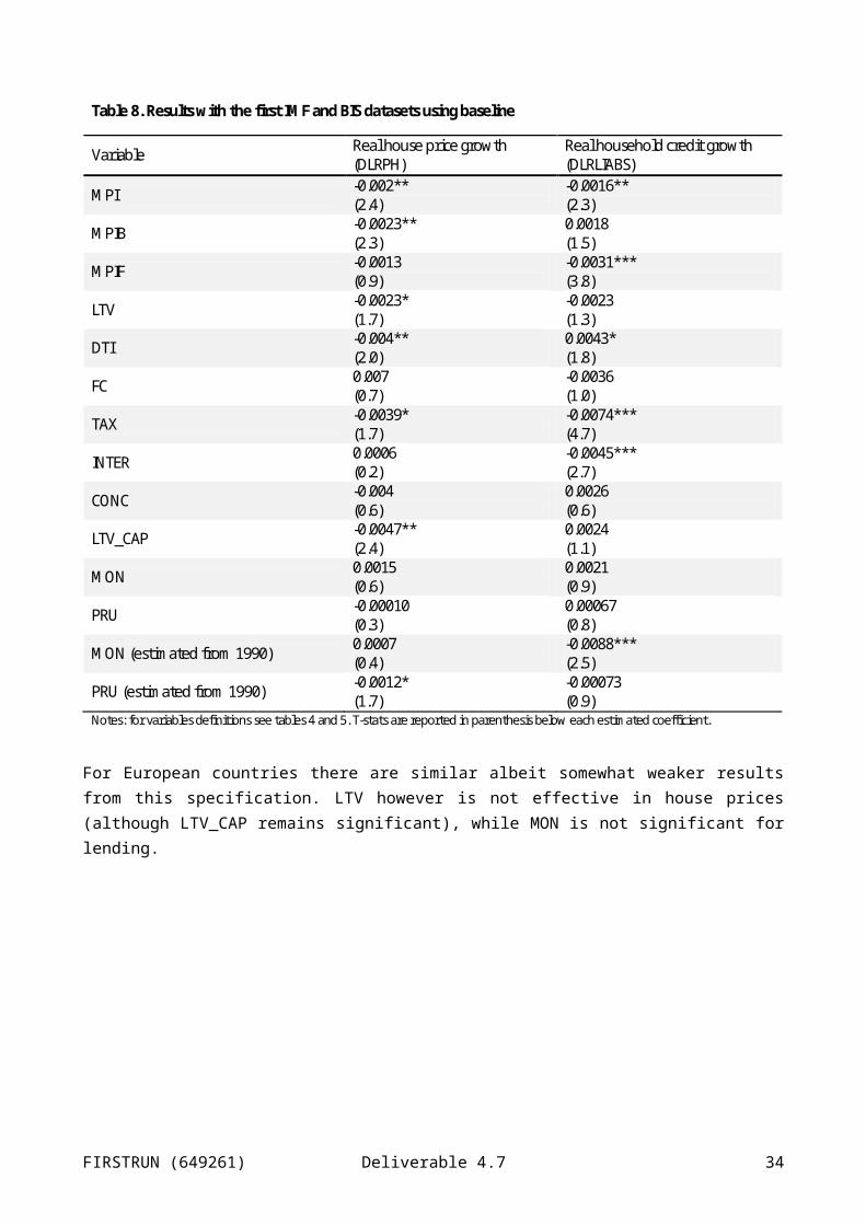
Table 20. Log real household credit, first stage: specification and test for stationarity

Countries Controls Sample period

Stationary residuals?

Australia log real house price, log housing stock, unemployment and log real disposable income

1990 onwards

**

Belgium log real house price, log housing stock, unemployment and log real disposable income 1980-2005 **

Canada log real house price, log housing stock, unemployment and log real disposable income 1990-2008 **

Denmark log real house price, log housing stock and log real disposable income 1996-2004 ***

Finland log real house price, log housing stock, unemployment and log real disposable income

2000 onwards

**

France log real house price, log housing stock, unemployment and log real disposable income

1970 onwards

***

Germany log real house price, log housing stock, unemployment and log real disposable income

2000 onwards

***

Greece log real house price, log housing stock, unemployment and log real disposable income

2000 onwards

**

Ireland log real house price, log housing stock, unemployment and log real disposable income 1970-2013 **

Italy log real house price, log housing stock, unemployment and log real consumer wage

2000 onwards

***

Japan log real house price, log housing stock, unemployment and log real disposable income

1980 onwards

**

Netherlands log real house price, log housing stock, unemployment and log real disposable income

1970 onwards

***

Norway log real house price, log housing stock and log real disposable income

2010 onwards

***

Austria log real house price, log housing stock, unemployment and log real disposable income

1970 onwards

**

Portugal log real house price, log housing stock and log real disposable income

1995 onwards

***

Sweden log real house price, log housing stock, unemployment and log real disposable income

1975 onwards

**

Spain log real house price, log housing stock, unemployment and log real disposable income

1971 onwards

**

UK log real house price, log housing stock, unemployment and log real disposable income

2010 onwards

**

US log real house price, log housing stock, unemployment and log real disposable income

2000 onwards

**

Notes: we have used the Augmented Dickey-Fuller test to test for stationary residuals. A *** means that the null hypothesis of non-stationarity is rejected at the 1 per cent significance level, a ** means the null is rejected at the 5 per cent level and a * at the 10

To account for possible short term deviations from the long-run relation we take an augmented equation that regresses real house price growth onto the residuals from the long-run relationship and a set of control variables in first differences. Results are presented in Table 21 for house price growth and Table 22 for real household credit growth. We estimate the system with a SUR procedure. The set of controls that we include in each regression is consistent with the control variables included in the panel regressions of Section 4. For some countries, such as for instance Belgium in the house price growth regressions, we have


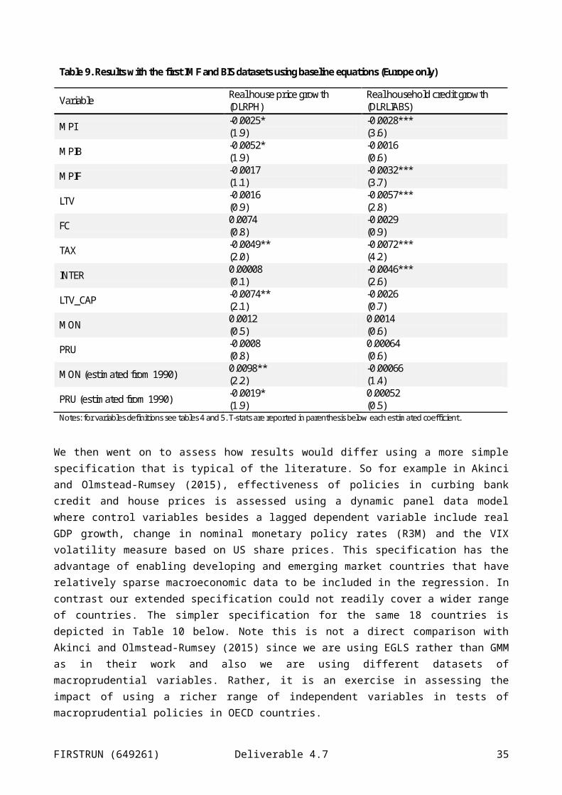
excluded some of the regressors as they turned out to be highly insignificant and reduced the adjusted R 2

statistic for that country. In addition, in some instances, such as Norway, we lacked data for some of the regressors.

From Table 21 we can see that the coefficients in front of the error correction term (the long-run relationship) are negative and significant in most instances, as expected. If there are deviations from the long-run relationship this term ensures that the dependent variable returns gradually to the long-run condition. We also obtain that house price growth depends positively on real income growth and, in most instances, negatively in the long term real interest rate.

From Table 22 we obtain again that the coefficient for the long-run relationship is negative for most countries and for those for which is not, is not statistically different than zero. Just as with house price inflation we also obtain that credit growth is positively related with income growth and negatively related with the long term real interest rate, although in several cases the latter control does not appear to be statistically different than zero.

The set of regressions presented in Table 21 and Table 22 constitute our baseline specifications upon which we add, one at a time, each of the macroprudential variables from the first IMF and BIS datasets. Given the short time span covered by the datasets, 2000Q1-2013Q4, it is often the case that some of the country macroprudential variables do not display any variation during the whole sample period. In Section 4 this was not a problem given the panel framework but in the SUR procedure this gives rise to singular matrices. In such instances we have excluded in each set of regressions all countries for which the macroprudential variable was constant. In addition, we omit the results of the regressions for which the coefficient on the macroprudential variable is not significantly different from zero for all the countries in the sample. Table 23 and Table 24 report the estimates of the effects of each macroprudential variable on real house price growth and household credit growth, respectively.

In both Table 23 and Table 24 we observe that whenever the coefficient is statistically different from zero, the effect goes, in most instances, in the expected direction: macroprudential variables reduce house price and credit growth. However, a large number of estimates are not statistically different from zero; a phenomenon that may be product of the binary nature of the underlying data.


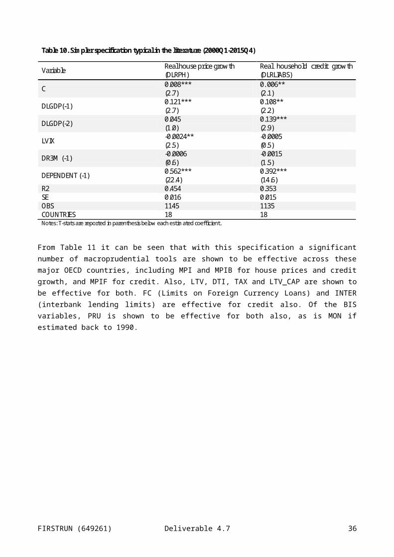
Table 21. Real house price growth, second stage: baseline equation

Australia Belgium Canada Denmark Finland France Germany Greece Ireland Italy

Constant-0.001 0.009 *** -0.002 0.000 0.004 * 0.003 ** -0.004 *** -0.01 0.002 -0.001

(0.003) (0.002) (0.001) (0.002) (0.002) (0.001) (0.001) (0.011) (0.002) (0.002)

Long run-0.081 *** -0.023 -0.050 *** -0.029 -0.241 *** -0.030 *** -0.246 *** -0.092 -0.046 ** -0.077 ***

(0.030) (0.020) (0.014) (0.027) (0.047) (0.008) (0.072) (0.172) (0.023) (0.022)

dlrph(-1)0.573 *** -0.062 0.649 *** 0.521 *** 0.398 *** 0.530 *** -0.136 0.022 0.288 *** 0.569 ***

(0.079) (0.094) (0.054) (0.067) (0.081) (0.056) (0.098) (0.186) (0.076) (0.063)

dlrr(-1)-0.006 * -0.003 -0.002 -0.006 * 0.003 -0.001 0.001 0.006 -0.006 ** 0.002

(0.003) (0.004) (0.001) (0.004) (0.004) (0.002) (0.003) (0.009) (0.003) (0.002)

dlrpdi±0.039 0.246 * 0.228 *** 0.155 ** 0.189 ** 0.087 0.292 *** 0.271 *** 0.114 0.379 ***

(0.089) (0.133) (0.053) (0.064) (0.092) (0.095) (0.099) (0.097) (0.075) (0.107)

drliabs(-1)0.175 -0.164 *** 0.003 -0.129 0.010 0.069 0.078 0.161 *** 0.154 **

(0.107) (0.025) (0.059) (0.095) (0.040) (0.102) (0.233) (0.059) (0.067)

dlrgw-0.008 -0.061 0.400 *** 0.254 *** 0.138 ** 0.000 -0.039 -0.036 0.084 0.081 *

(0.059) (0.059) (0.126) (0.047) (0.053) (0.030) (0.049) (0.029) (0.066) (0.042)

Du-0.004 -0.008 *** -0.004 -0.003 -0.009 *** 0.001 -0.019 *** -0.012 *** 0.002

(0.006) (0.002) (0.005) (0.005) (0.003) (0.004) (0.006) (0.004) (0.004)

Crisq-0.003 -0.009 ** -0.012 *** -0.006 0.010 -0.001 0.004 0.006 -0.019 *** -0.002

(0.005) (0.003) (0.003) (0.004) (0.008) (0.003) (0.007) (0.011) (0.005) (0.002)Adj. R2 0.31 0.01 0.69 0.70 0.38 0.46 0.11 0.39 0.57 0.59D-W 1.96 1.86 1.97 1.96 2.12 2.08 1.94 2.43 2.20 2.01


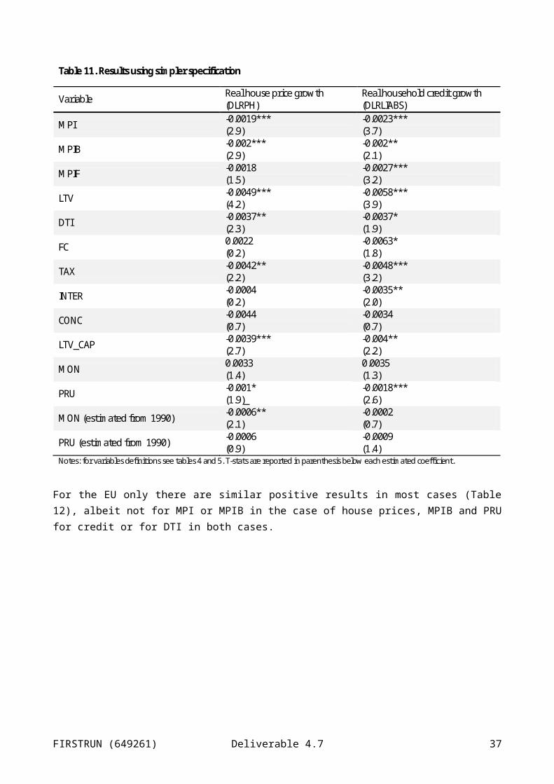
Japan Netherlands Norway Austria Portugal Sweden Spain UK US

Constant-0.002 ** 0.004 *** 0.004 0.005 ** -0.006 ** 0.001 0.004 0.002 0.003 **

(0.001) (0.002) (0.006) (0.002) (0.003) (0.002) (0.002) (0.002) (0.001)

Long run-0.01 ** -0.043 ** -0.377 ** -0.018 -0.633 *** -0.034 ** -0.038 *** -0.173 *** -0.061 ***

(0.005) (0.019) (0.187) (0.022) (0.138) (0.015) (0.013) (0.034) (0.018)

dlrph(-1)0.782 *** 0.356 *** 0.656 *** 0.003 0.317 ** 0.402 *** 0.606 *** 0.233 ** 0.354 ***(0.04) (0.104) (0.221) (0.066) (0.146) (0.065) (0.06) (0.091) (0.082)

dlrr(-1)-0.003 ** -0.004 -0.006 0.002 -0.004 -0.006 ** 0.003 0.004 -0.003

(0.001) (0.004) (0.018) (0.005) (0.006) (0.003) (0.002) (0.005) (0.002)

dlrpdi±0.201 *** 0.296 *** 0.807 *** 0.956 *** 0.008 0.428 *** 0.126 *** 0.396 *** 0.186 *(0.05) (0.073) (0.255) (0.102) (0.196) (0.076) (0.048) (0.13) (0.101)

drliabs(-1)-0.055 *** -0.018 -0.663 ** -0.032 0.09 -0.042 -0.015 0.275 * 0.113(0.02) (0.101) (0.294) (0.106) (0.1) (0.057) (0.084) (0.152) (0.074)

dlrgw0.14 *** 0.013 -0.013 0.137 0.129 *** 0.081 ** 0.11 * -0.015

(0.022) (0.01) (0.086) (0.262) (0.032) (0.033) (0.064) (0.03)

du0.004 -0.017 *** -0.029 *** 0.002 -0.008 * 0 -0.022 *** 0.002

(0.004) (0.006) (0.009) (0.004) (0.005) (0.003) (0.008) (0.003)

crisq-0.001 -0.006 0 0.005 -0.006 -0.009 ** -0.002 -0.011 ***

(0.001) (0.004) (0.006) (0.004) (0.004) (0.004) (0.004) (0.002)

Adj. R2 0.79 0.43 0.36 0.37 0.52 0.54 0.61 0.56 0.56

D-W 2.27 1.93 1.92 1.90 2.28 2.11 2.05 1.92 1.83Notes: Numbers in parenthesis are standard deviations. Long run are the residuals estimated from the first stage, dlrph is the change in log real house prices, dlrr is the change in the long term real rate, dlrpdi is the change in log real personal disposable income, dlrliabs is the change in log real household credit, dlrgw is the change in gross wealth, du is the change in unemployment rate and crisq is a crisis dummie. *** denotes that the coefficient is significant at the 1 per cent significance threshold a ** denotes significance at the 5 per cent threshold and a * denotes significance at the 10 per cent threshold. Adj. R2 denotes the adjusted R-squared statistic and D-W denotes the Durbin-Watson test for serial correlation of the residuals.±: for some countries we use dlrcwage instead, as specified in Table 19.


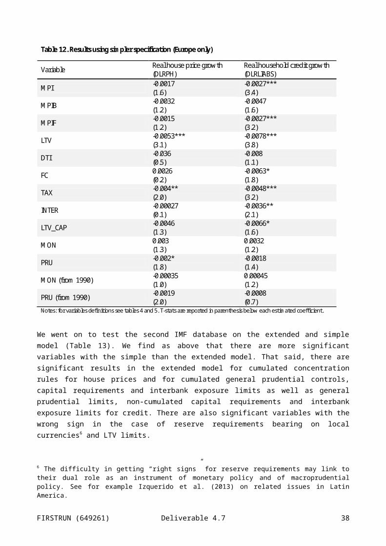
Table 22. Real household credit growth, second stage: baseline equation


Constant0.012 *** 0.005 *** 0.003 0.011 *** 0.005 ** 0.009 *** -0.001 ** 0.041 **

*-0.003 -0.007 **

(0.002)

(0.002)

(0.002)

(0.004) (0.002) (0.002)

(0.001)

(0.007) (0.004) (0.003)

Long run-0.101 *** -0.156 * -0.256 *** -0.4 ** -0.028 -0.024 -0.209 *** 0.045 -0.323 ** -1.08 ***(0.038

)(0.09) (0.073

)(0.204) (0.035) (0.021

)(0.065

)(0.078) (0.15) (0.221)

dlrliabs(-1)

0.223 *** -0.284 *** 0.302 *** -0.111 0.513 *** -0.004 0.368 *** -0.072 0.791 ***

-0.073(0.085

)(0.096

)(0.089

)(0.16) (0.086) (0.003

)(0.11) (0.139) (0.108) (0.12)

dlrr(-1)0.002 -0.007 * -0.004 * 0.005 0 0.208 0.002 -0.01 -0.002 -0.016 **

(0.002)

(0.004)

(0.002)

(0.008) (0.005) (0.193)

(0.003)

(0.006) (0.005) (0.008)

dlrpdi±0.018 0.368 ** 0.124 * 0.365 ** 0.287 *** 0.049 0.034 0.33 **

*0.217 **

*0.391 ***

(0.065)

(0.151)

(0.07) (0.157) (0.098) (0.053)

(0.072)

(0.107) (0.056) (0.141)

dlrgw0.136 *** 0.071 * 0.508 *** 0.32 *** 0.091 ** -0.004 -0.02 -0.043 0.274 **

*0.007

(0.042)

(0.037)

(0.159)

(0.099) (0.044) (0.005)

(0.049)

(0.027) (0.093) (0.071)

Crisq-0.007 * -0.421 11.272 *** 1.763 21.76 0.009 -0.001 -0.027 **

*0.001 0.009 **

(0.004)

(1) (5.11) (1.187) (23.178) (0.002)

(0.001)

(0.009) (0.005) (0.003)Adj. R2 0.18 0.21 0.22 0.36 0.34 0.0 0.07 0.50 0.75 0.49D-W 2.06 1.80 1.78 1.86 2.21 2.04 2.06 1.87 1.71 1.47


Japan Netherlands Norway Austria Portugal Sweden Spain UK US

Constant0.017 *** 0.007 *** 0.009 *** 0.003 *** 0.001 0.005 *** 0.007 *** 0 0.004 **

(0.002)

(0.002)

(0.003)

(0.001) (0.002) (0.002)

(0.002)

(0.001) (0.001)

Long run-0.209 *** -0.021 -0.892 *** -0.035 -0.015 -0.073 *** -0.034 * 0.165 -0.092 *(0.058

)(0.018

)(0.189

)(0.023) (0.024) (0.025

)(0.018

)(0.16) (0.048)

dlrliabs(-1)

0.11 0.034 0.084 -0.055 0.643 *** -0.027 0.224 *** -0.007 0.627 ***(0.078

)(0.065

)(0.128

)(0.052) (0.061) (0.059

)(0.069

)(0.121) (0.075)

dlrr(-1)0 -0.006 ** 0.005 0.004 0.004 -0.002 0 0.013 0.001

(0.003)

(0.003)

(0.01) (0.003) (0.003) (0.003)

(0.002)

(0.009) (0.003)

dlrpdi±0.202 ** 0.48 *** 0.514 *** 0.605 *** 0.46 *** 0.364 *** 0.055 0.121 * 0.01(0.09) (0.059

)(0.127

)(0.054) (0.131) (0.088

)(0.044

)(0.069) (0.085)

dlrgw0.058 -0.006 0.125 *** 0.462 *** 0.261 *** 0.132 *** 0.244 **

*0.046

(0.05) (0.011)

(0.045) (0.129) (0.037)

(0.029)

(0.04) (0.032)

Crisq-0.017 *** 0.005 0.002 -0.005 * -0.005 -0.007 ** -0.012 **

*-0.005 **

(0.003)

(0.005)

(0.003) (0.003) (0.004)

(0.003)

(0.003) (0.002)

Adj. R2 0.34 0.25 0.56 0.49 0.84 0.32 0.30 0.70 0.62D-W 2.06 1.62 1.55 2.13 1.78 1.86 2.01 1.76 2.31Notes: Numbers in parenthesis are standard deviations. Long run are the residuals estimated from the first stage, dlrliabs is the change in log real household credit, dlrr is the change in the long term real rate, dlrpdi is the change in log real personal disposable income, dlrgw is the change in gross wealth and crisq is a crisis dummie. *** denotes that the coefficient is significant at the 1 per cent significance threshold a ** denotes significance at the 5 per cent threshold and a * denotes significance at the 10 per cent threshold. Adj. R2 denotes the adjusted R-squared statistic and D-W denotes the Durbin-Watson test for serial correlation of the residuals. ±: for some countries we use dlrcwage instead, as specified in Table 20.


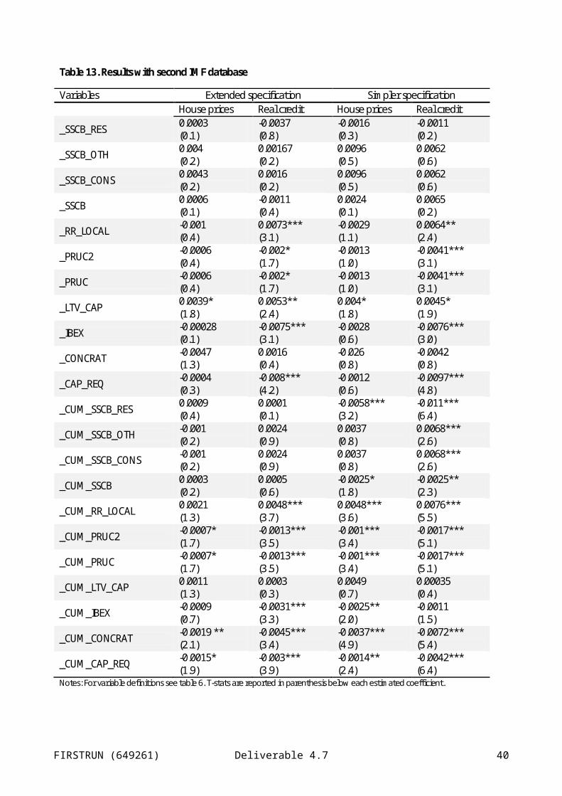
Table 23. Real house price growth: impact of macroprudential variables


MPI -0.0026 * -0.0101 0.0008(0.0014) (0.007) (0.0036)

MPIB -0.0026 *(0.0013)

MPIF -0.0099 0.0002(0.0071

)(0.0036)

LTV -0.0054 ** -0.0019 -0.0023(0.0027) (0.0047

)(0.0025

)TAX -0.0089 0.0001

(0.0072)

(0.0036)

LTV_CAP -0.0052 *(0.0027)

MON -0.0014 0.0002 0.0013 -0.0017 0.0003 0.0324 ** -0.0013 0.0000(0.0024

)(0.0005) (0.0039

)(0.0013) (0.0006) (0.016) (0.001) (0.0004

)PRU 0.0034 0.0011 0.0015 -0.0007 0.0025 -0.0002

(0.0022)

(0.0007) (0.005) (0.0039) (0.0032) (0.0044)


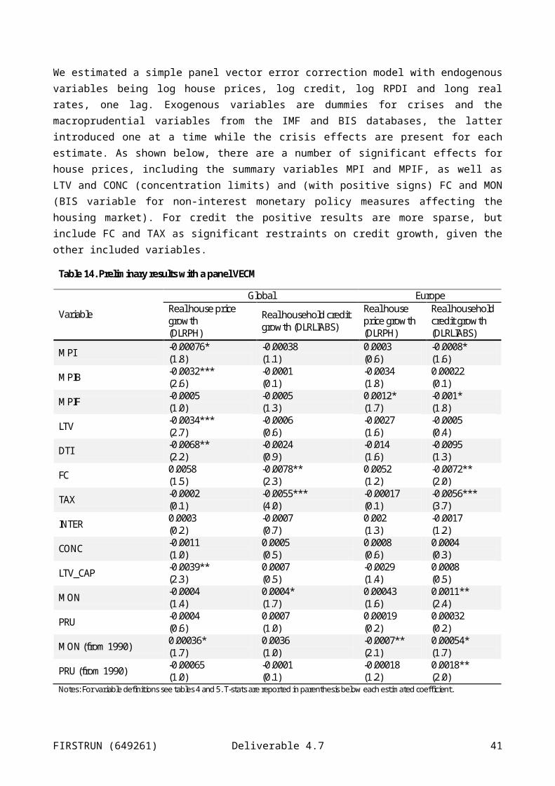
Japan Netherlands Norway Austria Portugal Sweden Spain US

MPI -0.0054 ** -0.0155 *** 0.0070 -0.0026 -0.0097 * 0.0083(0.0027

)(0.0044) (0.0048

)(0.0027

)(0.0058) (0.0056

)MPIB -0.0043 -0.0101

(0.0038)

(0.0061)

MPIF -0.0189 *** -0.0156 *** 0.0080 * -0.0028 0.0073(0.0067

)(0.0044) (0.0049

)(0.0027

)(0.0056

)LTV -0.0092 -0.0084

(0.0077)

(0.006)TAX -0.0181 *** 0.0139 -0.0010

(0.0067)

(0.01) (0.0042)

LTV_CAP -0.0086 -0.0101(0.0077

)(0.0061)

MON -0.0014 -0.0004 -0.0011 -0.0069 -0.0020 0.0005(0.0012

)(0.0033

)(0.0047

)(0.0072

)(0.0035) (0.0022

)PRU -0.0048 ** -0.0116 0.0037 * 0.0046

(0.002) (0.021) (0.0022) (0.0037)

Notes: For variable definitions see Table 4 and Table 5. Numbers in parenthesis are standard deviations. *** denotes that the coefficient is significant at the 1 per cent significance threshold a ** denotes significance at the 5 per cent threshold and a * denotes significance at the 10 per cent threshold.


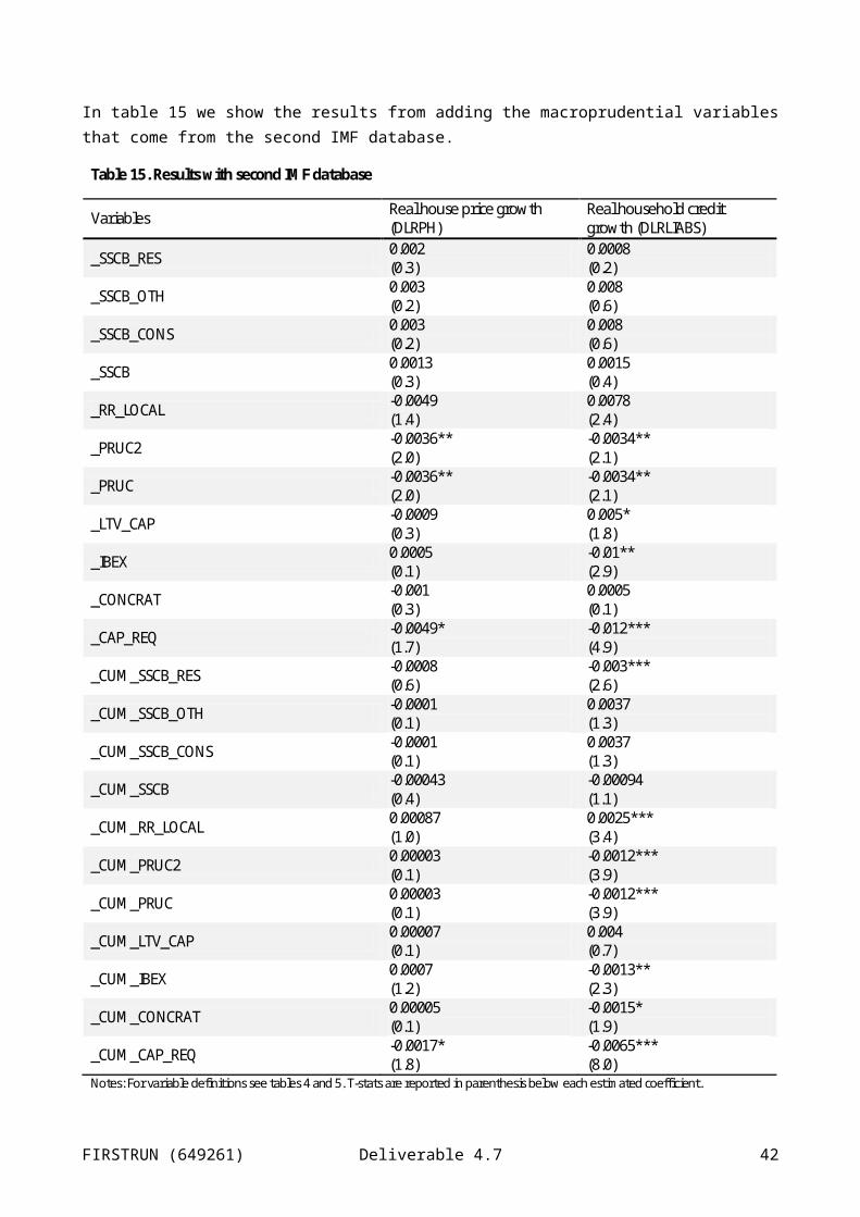
Table 24. Real household credit growth: impact of macroprudential variables

Australia Belgium Canada Denmark Finland France Germany Greece Ireland ItalyMPI 0.0022 -0.0125 ** -0.0141 ** 0.0005

(0.0014)

(0.0048)

(0.0059)

(0.0006)MPIB

MPIF -0.0122 ** -0.0138 ** 0.0006(0.0049

)(0.006) (0.0006

)LTV

TAX -0.0135 ***

-0.0148 ** 0.0004(0.0052

)(0.0065

)(0.0014

)LTV_CAP

MON 0.0021 -0.0016 ***

0.0067 -0.0028 -0.0019 0.0124 0.0000 0.0139 ***(0.0043) (0.0006

)(0.0072

)(0.0019

)(0.0034

)(0.0146

)(0.007) (0.0046

)PRU -0.0070 **

0.0019 -0.0189 -0.0053 0.0073 0.0015(0.0014

)(0.0054

)(0.0136

)(0.0046

)(0.015) (0.026)


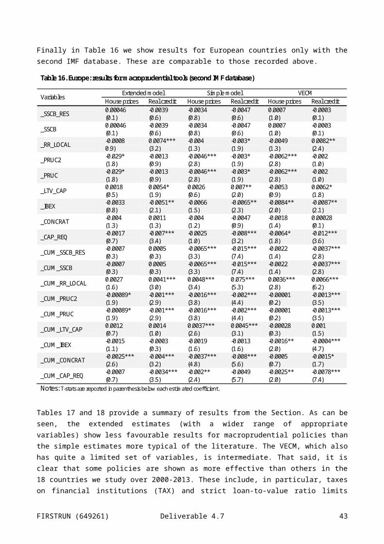
Japan Netherlands Norway Austria Portugal Sweden Spain USMPI -0.0049 -0.0043 * -0.0031 * -0.0056 ** -0.0031 -0.005

(0.0032) (0.0021)

(0.0016)

(0.0027)

(0.0043)

(0.0043)MPIB -0.0026 -0.0047

(0.0058) (0.0045)MPIF -0.0096 * -0.0044 ** -0.0031 * -0.0053 * -0.006

(0.0057) (0.0021)

(0.0016)

(0.0028)

(0.0043)LTV -0.0051 -0.0047

(0.0115) (0.0045)TAX -0.0088 -0.0077 *

*(0.0063) (0.0033)LTV_CAP -0.0034 -0.0045

(0.0115) (0.0045)MON 0.0007 0.0041 -0.0014 0.0066 ** -0.0145 **

*(0.0031) (0.0028) (0.002) (0.0032)

(0.0032)PRU -0.0050 *

*-0.0170 **

*-0.0060 ** 0.0099 **

*0.0066 **

(0.0022) (0.0055)

(0.0031)

(0.0033)

(0.003)

Notes: For variable definitions see Table 4 and Table 5. Numbers in parenthesis are standard deviations. *** denotes that the coefficient is significant at the 1 per cent significance threshold a ** denotes significance at the 5 per cent threshold and a * denotes significance at the 10 per cent threshold.


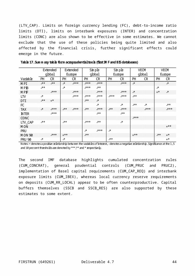
6 ConclusionsMacroprudential policy is focused on the financial system as a whole, with a view to limiting macroeconomic costs from financial distress (Crockett 2010), with risk taken as endogenous to the behaviour of the financial system. However, “analysis is still needed about the appropriate macroprudential tools, their transmission mechanism and their effect” (Galati and Moessner 2014). Theoretical models are in their infancy and empirical evidence on the effects of macroprudential tools is still scarce. Nor has a primary instrument for macroprudential policy emerged.

Accordingly, in this paper we have provided an overview of the state of the art in macroprudential tools, transmission and modelling before undertaking some testing of tools on a dataset of up to 19 OECD countries during 2000-2014, using available global databases (from the IMF and the BIS). We contend that extant empirical evidence is often unsatisfactory in the sense of omitting important control variables (for understandable reasons since these variables are simply unavailable for all but the most advanced countries), leading to excessively favourable results for the impact of macroprudential policies in OECD countries, and show the impact of this in terms of different specifications.

Nevertheless, overall, it is clear that some policies are shown as more effective than others in the up to 19 countries we study over 2000-2014. These include, in particular, taxes on financial institutions, general capital requirements and strict loan-to-value ratio limits. Limits on foreign currency lending, debt-to-income ratio limits, limits on interbank exposures and concentration limits are also shown to be effective in some estimates.

We contend that the way forward for reduced form modelling is a more sophisticated form of the baseline equations such as we include here. There could also be an assessment of the impact of macroprudential tools on a wider range of variables than credit and house prices. These could include for example spreads on loans, as shown in Appendix C. However, a potential issue is that the impact of macroprudential policies on the cost of lending is ambiguous, at least for some policies, since they may on the one hand raise bank costs, tending to widen the spread, but also reduce bank risk, tending to narrow it.

7 ReferencesAcharya, V. V. (2013), "Adapting Micro Prudential Regulation for Emerging Markets", Dealing with the Challenges of Macro Financial Linkages in Emerging Markets, 57.

Adams, Z. and Füss, R. (2012) “Disentangling the short and long-run effects of occupied stock in the rental adjustment process”. The Journal of Real Estate Finance and Economics, 44(4), 570-590.

Aikman, D., Alessandri, P., Eklund, B., Gai, P., Kapadia, S., Martin, E., Mora, N., Sterne, G. and Willison, M. (2009), "Funding Liquidity Risk in a Quantitative Model of Systemic Stability", Bank of England Working Paper 372.

Aiyar, S., Calomiris, C. W. and Wieladek, T. (2014), "Does macro-prudential regulation leak? Evidence from a UK policy experiment", Journal of Money, Credit and Banking, 46(1), pp. 181-214.

Akinci, O. and Olmstead-Rumsey, J. (2015), “How effective are macroprudential policies? An empirical investigation”, International Finance Discussion Papers 1136.


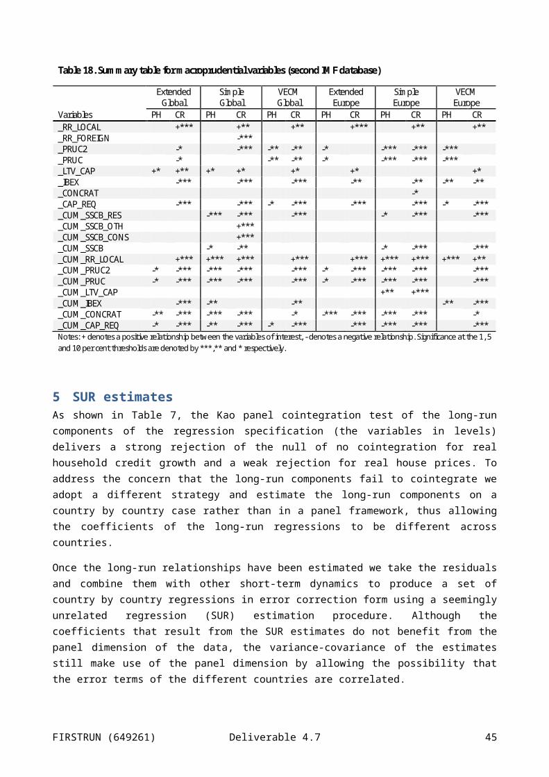
Angelini, P., Neri, S. and Panetta, F. (2010), “Grafting macroprudential policies in a macroeconomic framework; choice of optimal instruments and interaction with monetary policy”, paper presented at a conference on “Procyclicality and Financial Regulation”, Tilburg, 11-12 March 2010.

Angeloni, I. and Faia, E. (2009), “A tale of two policies, prudential regulation and monetary policy with fragile banks”, Kiel Working Paper 1569, Kiel Institute for the World Economy.

Antipa, P., Mengus, E. and Mojon, B. (2010), "Would macroprudential policy have prevented the Great Recession?", Manuscript, Banque de France.

Antipa, P. and Matheron, S. (2014), “Interactions between monetary and macroprudential policies”, Banque de France Financial Stability Review, 18, pp. 225-239.

Armstrong, A. and Davis, E. P. (2014), “Comparing housing booms and mortgage supply in the major OECD countries”, National Institute Economic Review, November, R3-R15.

Arregui, N., Beneš, J., Krznar, I. and Mitra, S. (2013), “Evaluating the net benefits of macroprudential policy: A cookbook.”, IMF Working Paper No. 13/167.

Barrell, R., Davis, E. P., Fic, T., Holland, D., Kirby, S. and Liadze, I. (2009), “Optimal regulation of bank capital and liquidity: how to calibrate new international standards” FSA Occasional Paper no. 38, October.

Barrell, R., Davis, P., Karim, D., Liadze, I., (2010a), “Bank regulation, property prices and early warning systems for banking crises in OECD countries”, Journal of Banking and Finance, 34, pp. 2255–2264.

Barrell, R., Davis, E., Karim, D. and Liadze, I. (2010b), "Calibrating macroprudential policy", NIESR Discussion Paper No. 354.

Barrell, R., Kirby, S. and Riley, R. (2004), “The current position of UK house prices”. National Institute Economic Review, (189), 57-60.

Barrell, R., Kirby, S. and Whitworth, R. (2011), “Real house prices in the UK”. National Institute Economic Review, 216(1), F62-F68.

Basel Committee (2010), “Countercyclical capital buffer proposal - consultative document”, BIS, Basel, July 2010.

Basel Committee (2011), “Basel III: A global regulatory framework for more resilient banks and banking systems”, BIS, Basel, June 2011.

Benes, J., Kumhof, M. and Laxton, D. (2014b), "Financial Crises in DSGE Models: Selected Applications of MAPMOD", IMF Working Paper WP/14/56, April.

Benigno, G., Chen, H., Otrok, C., Rebucci, A. and Young, E. (2013), "Financial Crises and Macro-Prudential Policies", Journal of International Economics, 89(2), pp. 453-470.

Bennani, T., Després, M., Dujardin, M., Duprey, T. and Kelber, A. (2014), “Macroprudential framework: key questions applied to the French case”, Banque de France Occasional papers, No. 9

Berg, S. A. (1993), “The Banking Crisis in the Scandinavian countries”, in “FIDICIA, an appraisal”, FRB Chicago Banking Conference Proceedings, 441-9.

Bernanke, B., Gertler, M. and Gilchrist, S. (1999), "The financial accelerator in a quantitative business cycle framework", Handbook of Macroeconomics 1 (1999), pp. 1341-1393.


Boissay, F., Collard, F. and Smets, F. (2013), "Booms and systemic banking crises", ECB Working Paper No. 1514.

Borio, C. and Drehmann, M. (2009), "Towards an operational framework for financial stability: ‘fuzzy’ measurement and its consequences", BIS Working Paper No. 284.

Borio, C. and Shim, I. (2007) "What can (macro-)prudential policy do to support monetary policy?", BIS Working Paper No. 242.

Bruno, V., Shim, I. and Shin, H. S. (2015), “Comparative assessment of macroprudential policies”, BIS Working Paper No. 502.

Brunnermeier, M. and Sannikov, Y. (2014), "A Macroeconomic Model with a Financial Sector", American Economic Review, 104(2), pp. 379-421.

Capozza, D. R., Hendershott, P. H., Mack, C. and Mayer, C. J. (2002), “Determinants of real house price dynamics”. National Bureau of Economic Research, No. 9262.

Catte, P., Cova, P., Pagano, P. and Visco, I. (2010), "The role of macroeconomic policies in the global crisis", Bank of Italy Occasional Papers No. 69.

Cerutti, E., Claessens, S. and Laeven, L., (2015), ”The Use and Effectiveness of Macroprudential Policies: New Evidence”, IMF Working Paper 15/61.

Cerutti, E., Correa, R., Fiorentino, E. and Segalla, E. (2016), “Changes in prudential policy instruments, a new cross country database”, IMF Working Paper 16/110.

CGFS (2010), “Macroprudential instruments and frameworks: report published by the Committee on the Global Financial System” 21 May 2010, Basel.

Claessens, S., Ghosh, S. R. and Mihet, R. (2014), “Macroprudential policies to mitigate financial system vulnerabilities”, IMF Working Paper 14/155.

Crockett, A. (2000), "Marrying the micro- and macro-prudential dimensions of financial stability", Remarks before the Eleventh International Conference of Banking Supervisors. Bank for International Settlements. Basel, 20-21 September 2000.

Crowe, C. W., Dell'Ariccia, G., Igan, D. and Rabanal, P. (2011), “How to Deal with Real Estate Booms: Lessons from Country Experiences” IMF Working Paper No. 11/91.

Darbar, S. M. and Wu, X. (2015), “Experiences with macroprudential policy, five case studies”, IMF Working Paper 15/123.

Davis, E. P., Fic, T. M. and Karim, D. (2011), “Housing Market Dynamics and Macroprudential Tools”, in “RUTH, the Riksbank’s inquiry into the risks in the Swedish housing market” pages 219-298, also Brunel Economics and Finance Working Paper 11-07.

Dell’Ariccia, G., Igan, D., Laeven, L. and Tong, H. (2012), “Policies for Macrofinancial Stability: Options to Deal with Credit Booms,” IMF Staff Discussion Note 12/06.

De Nicolò, G., Favara, G. and Ratnovski, L. (2012), “Externalities and Macroprudential Policy”, IMF Staff Discussion Note 12/05.

Diamond, D. and Dybvig, P. (1983), "Bank runs, deposit insurance, and liquidity", Journal of Political Economy, 91(3), pp. 401–419.


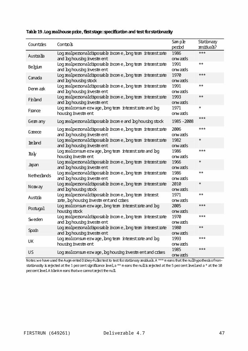
Drehmann, M. (2009), "Macroeconomic Stress Testing Banks: A Survey of Methodologies", Stress Testing the Banking System: Methodologies and Applications, ed. M. Quagliariello. Cambridge, Cambridge University Press.

Engle, R. F. and Granger, C. W. (1987), "Co-integration and error correction: representation, estimation, and testing", Econometrica: journal of the Econometric Society, 251-276.

Fisher, I. (1933), "The debt-deflation theory of great depressions", Econometrica: Journal of the Econometric Society, 337-357.

Galati, G. and Moessner. R. (2014), “What do we know about the effects of macroprudential policy?” DNB Working Paper No. 440.

Gali. J, (2009), “Monetary policy, inflation and the business cycle”, Princeton University Press.

Gauthier, C., Lehar, A. and Souissi, M. (2012), "Macroprudential capital requirements and systemic risk", Journal of Financial Intermediation, 21(4), pp. 594–618.

Gerlach, S. and Peng, W. (2005), “Bank lending and property prices in Hong Kong”, Journal of Banking and Finance, 29, pp. 461-481.

Gersbach, H. and Rochet, J. C. (2012a), "Capital Regulation and Credit Fluctuations", CEPR Discussion Paper No. 9077.

Gersbach, H. and Rochet, J. C. (2012b), "Aggregate Investment Externalities and Macroprudential Regulation", Journal of Money, Credit and Banking, 44, pp. 73-109.

Goodfriend, M. and McCallum, B. (2007), "Banking and interest rates in monetary policy analysis: a quantitative exploration", Journal of Monetary Economics, 54, pp. 1480–1507.

Goodhart, C. A. E. (2010), “Money, credit and bank behaviour: need for a new approach” National Institute Economic Review, 214.

Goodhart, C., Kashyap, A., Tsomocos, D. and Vardoulakis, A. (2012), "Financial Regulation in General Equilibrium", NBER Working Paper No. 17909.

Goodhart, C., Kashyap, A., Tsomocos, D. and Vardoulakis, A. (2013), "An Integrated Framework for Analyzing Multiple Financial Regulations", International Journal of Central Banking, 9(1), pp. 109-143.

He, Z., and Krishnamurthy, A. (2014), "A macroeconomic framework for quantifying systemic risk", NBER Working Paper 19885.

Horváth, B. and Wagner, W. (2013), "The Disturbing Interaction between Countercyclical Capital Requirements and Systemic Risk", Mimeo, Tilburg University.

Igan, D. and Loungini, P. (2012), “Global house price cycles”. IMF Working Paper WP/12/217.

Igan, D, and Kang, H. (2011), “Do Loan-to-Value and Debt-to-Income Limits Work? Evidence from Korea,” IMF Working paper 11/297.

Izquerido, A., Loo-Kung, R. and Rojas-Suarez, L. (2013), ”Macroprudential Regulations in Central America”, Center for Global Development, Working Paper No 318.

IMF (2012), “The Interaction of Monetary and Macroprudential Policies”, IMF Board Paper and Background Paper.


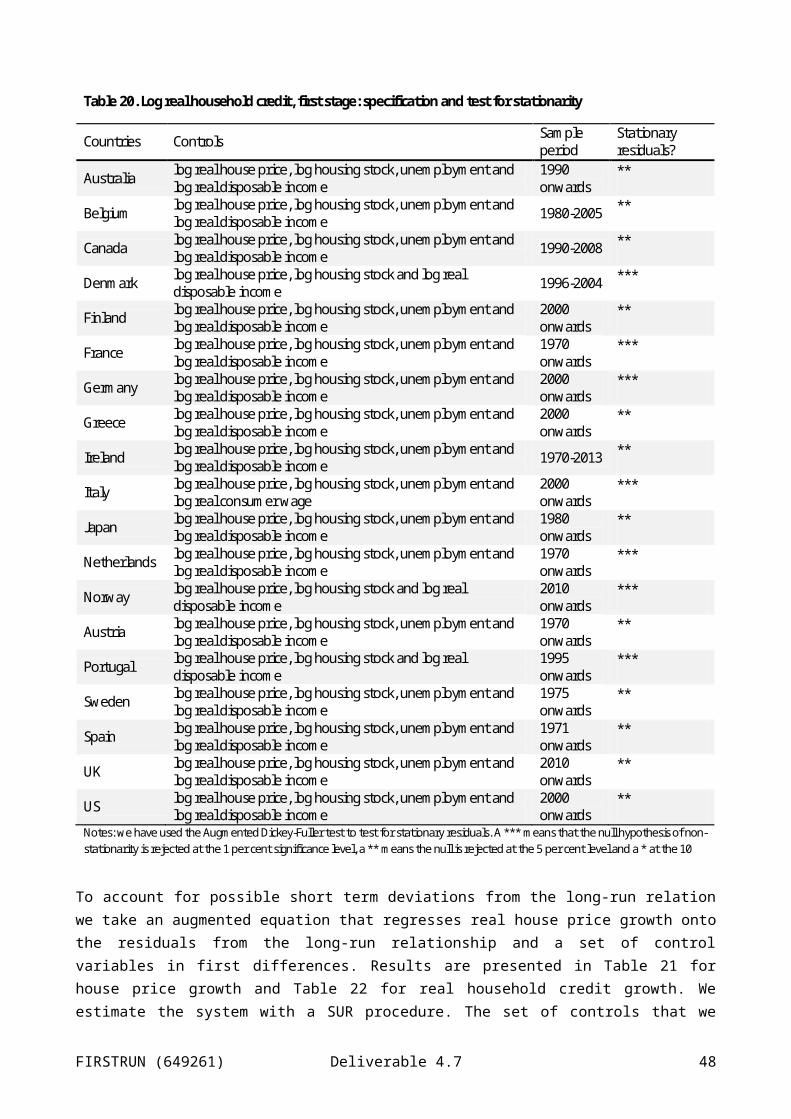
IMF (2013), “Key aspects of macroprudential policy – background paper”, IMF policy paper.

Jiménez, G., Ongena, S., Peydró, J. L., & Saurina Salas, J. (2012), “Macroprudential Policy, Countercyclical Bank Capital Buffers and Credit Supply: Evidence from the Spanish Dynamic Provisioning Experiments,” National Bank of Belgium Working Paper 231.

Kannan, P., Rabanal, P. and Scott, A. (2012), "Monetary and Macroprudential Policy Rules in a Model with House Price Booms", The B.E. Journal of Macroeconomics, 12(1).

Kao, C. (1999), “Spurious Regression and Residual-Based Tests for Cointegration in Panel Data”, Journal of Econometrics, 90, pp. 1-44.

Kashyap, A. K., Tsomocos, D.P. and Vardoulakis, A.P. (2014), "How does macroprudential regulation change bank credit supply?", NBER Working Paper No. 20165.

Kuttner, K, N., and Shim, I. (2013), “Can non-interest rate policies stabilise housing markets? Evidence from a panel of 57 economies,” BIS Working Paper No 433.

Lim, C.H., Columba, F., Costa, A., Kongsamut, P., Otani, A., Saiyid, M, Wezel, T. and Wu, X. (2011), “Macroprudential Policy: What Instruments and How to Use Them? Lessons from Country Experiences,” IMF Working Paper 11/238.

Maddaloni, A. and Peydro, J. L. (2013) "Monetary policy, macroprudential policy and banking stability: evidence from the Euro Area", International Journal of Central Banking, 9(1), p. 121-169.

McCauley, R. (2009), “Macroprudential tools in emerging markets”, Paper written for Central Bank of Nigeria‘s 50th Anniversary International Conference on "Central banking, financial system stability and growth“, session on “Rethinking regulation for financial system stability and growth”, Abuja, 4-9 May 2009.

Meen, G. (2002), “The time-series behavior of house prices: a transatlantic divide?”, Journal of housing economics, 11(1), 1-23.

Meh, C. and Moran, K. (2008), “The role of bank capital in the propagation of shocks”, Bank of Canada working paper No 2008-36.

Muellbauer, J. and Murphy, A. (2008), “Housing markets and the economy: the assessment”. Oxford review of economic policy, 24(1), 1-33.

Perotti, E. and Suarez, J. (2011), "A Pigovian Approach to Liquidity Regulation", International Journal of Central Banking, 7(4), pp. 3-41.

Saurina, J. (2009), “Dynamic provisioning, the experience of Spain”, Crisis Response Note No 7, World Bank.

Shim, I., Bogdanova, B., Shek, J. and Subelyte, A. (2013), "Database for policy actions on housing markets", BIS Quarterly Review, September, 83-95.

Vandenbussche, J., Vogel, U., and Detragiache, E. (2012), "Macroprudential Policies and Housing Prices—A New Database and Empirical Evidence for Central, Eastern, and Southeastern Europe", IMF Working Paper No. 12/303.

Van den End, J.W. (2012) "Liquidity Stress-Tester: Do Basel III and unconventional monetary policy work?", Applied Financial Economics, 22(15), pp. 1233–57.

Weale, M. (2008), “Commentary: the banking crisis and the economy”. National Institute Economic Review, 204(1), 4-8.


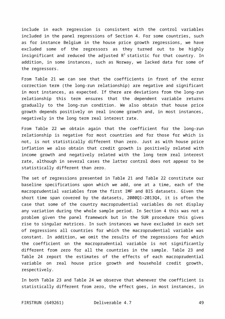
Wong, E., Fong, T., Li K., and Choi, H. (2011), "Loan-to-value ratio as a macro-prudential tool – Hong Kong’s experience and cross-country evidence", Hong Kong Monetary Authority Working Paper No.1.

Wong, E. and Hui, C.-H. (2010), “Loan-To-Value Ratio As A Macro-Prudential Tool –Hong Kong Experiences”, mimeo, Research Department, Hong Kong Monetary Authority

Woodford, M. (2010), “Financial intermediation and macroeconomic analysis”, Journal of Economic Perspectives, 24(4), pp. 21–44.

Zhang, L. and Zoli, E. (2014), “Leaning Against the Wind: Macroprudential Policy in Asia,” IMF Working Paper 14/22.

8 Appendix A: selected national experiences of macroprudential policiesHong Kong has no scope for raising interest rates due to the fixed rate vis a vis the US dollar. Accordingly, macroprudential instruments were seen as essential to prevent banking crises following property bubbles when the US interest rate was “too high” for domestic conditions in Hong Kong. There were successive decreases in the maximum loan to value ratio in the 1990-7 period, from 80-90 per cent to 60 per cent. Although the Asian crisis came after the last tightening, with a marked fall in the price of housing, the banks remained solvent given the low LTVs on their loans. This limit was complemented by a maximum limit of 40 per cent of assets to be held in the form of mortgage loans over 1994-8.

Wong and Hui (2010) comment that although property prices dropped remarkably by more than 40 per cent right after the Asian financial crisis, the subsequent delinquency ratio for mortgages in Hong Kong never exceed 1.43 per cent. They also suggest that a policy of mortgage insurance may need to be instituted to prevent excessive liquidity constraints on households and that that an effective operation of loan-to-value policy may require some discretion to adjust the maximum loan-to-value ratio.

Gerlach and Peng (2005) showed that the limits on LTVs had a detectable effect on the impact of house prices on borrowing in Hong Kong, with a 10 per cent rise in house prices having only a 1.5 per cent effect on lending compared to per4per cent before the measures. In earlier work (Gerlach and Peng 2002) they showed that there is both short-term and long-term causality running from property prices to lending but not the opposite, suggesting that the LTV limits did not restrain property prices per se.

Darbar and Wu (2015) note that in 2014 the Hong Kong banking sector faced risks again from elevated property prices, spillovers from the expected exit from low interest rates and increasing integration with China. The rise in property prices was driven by lack of housing supply and increased mortgage lending, including demand from mainland China. This followed a good performance in the global financial crisis, as banks were not exposed to securitised products, had strong internal liquidity, good risk management and low loan to deposit ratios. Macroprudential policy was tightened beginning in 2009, with particular focus on LTV and DSTI measures. There is evidence that the tightening enhanced the resilience of the banking sector and limited household leverage, although house prices recommenced their ascent in 2014, as did mortgage lending. Taxes on property transactions may have had a larger impact. In 2015 the rise in the credit to GDP ratio prompted a counter cyclical buffer, capital conservation buffer.

Darbar and Wu (2014) show that, the Netherlands, facing rising house prices and bank lending is reported to have imposed a cap on LTVs followed by gradual reductions in them, by law, with a target of 100 per cent which is still high by international standards. Meanwhile, maximum LTI limits were imposed on


mortgage loans and the tax deductibility limited. Additional capital buffers were imposed on the largest banks.

Sweden imposed an LTV limit in 2010 for the first time, of 85 per cent, followed in 2013 by a risk-weight floor of 15 per cent for mortgages, which was recently increased to 25 per cent. This is for banks that use the IRB approach to risk assessment. Mandatory amortisation schedules were imposed in 2014, with loans having to be repaid at least 2 per cent a year if the LTV is over 70 per cent and 1 per cent a year if it is over 50 per cent. LCRs were imposed early, and capital ratios are higher than Basel III requires for the largest banks. Finally a counter cyclical buffer came into force in 2015

Outside Europe, New Zealand limited the share of high LTV housing loans in 2013. Singapore, like Hong Kong, limited LTVs and DSTIs as well as having loan tenor rules, measures on auto loans and unsecured credit. The effect was to lower LTVs and lead to a reduction in house prices in 2013-14.


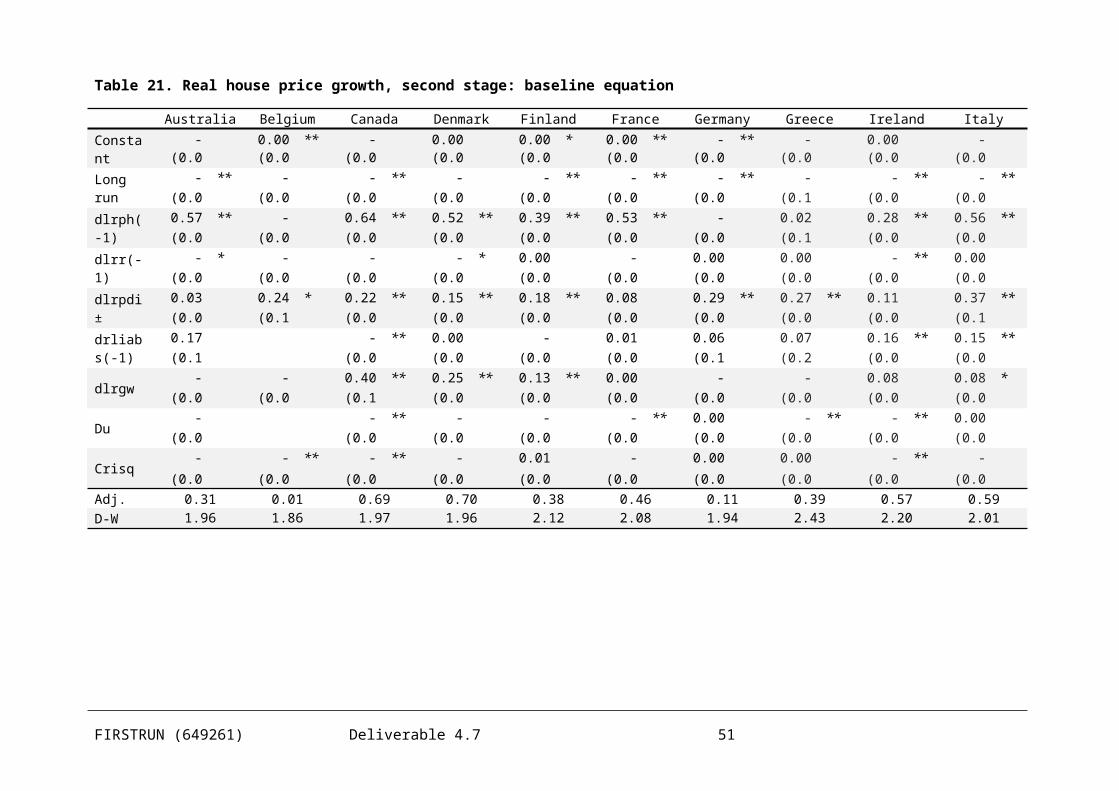
9 Appendix B: summary of the literatureTable 25.Existing empirical studies

Study Dependent MP variables Method Date of sample Key result

Crowe et al. (2011)

Real estate booms and busts

LTV, Property taxes

Time series (US regions), cross section (international), DSGE model

US 1978-2008, international 2000-7

LTV is effective for house prices

Borio and Shim (2007)

Credit and asset price growth

General dummy for MP measures

Authorities' assessment. Regression in double and single difference, controls are GDP growth, policy rate

[1988]-2006, 22 countries

MP measures effective in reducing credit and house price growth

Wong et al. (2011)

Mortgage delinquency ratios

LTV

Panel; controls include property prices, GDP growth, mortgage debt/GDP and interest rates).

1991-2010, 13 countries unbalanced panel

Economies with LTV policy are estimated to have a lower sensitivity of mortgage delinquency ratios to property prices than those without LTV policy

Kuttner and Shim (2013)

Growth in house prices and housing credit

DTI, LTV, TAXPanel regression, controls are interest rate and growth in GNI per capita

2000-12, 57 countries

DTI, LTV and TAX affect housing credit but only TAX affects house price growth

Lim et al. (2011)

Private sector credit and leverage

RR, DP, LTV, DTI, DP, CCC, FC Panel GMM regression 2000-2010,

49 countriesMP Policies can affect credit growth and leverage, especially LTV, DTI, CG, RR, DP


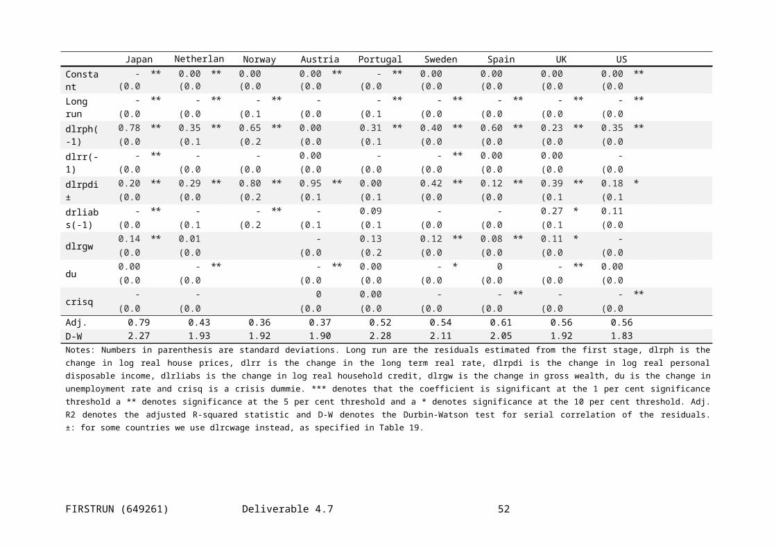
Van den Bussche et al. (2012)

House price growth CR, RR Panel regression

16 CEE countries, 2002-11

CR and RR help slow house prices


Akinci and Olmstead-Rumsey (2015)

Bank credit, housing credit and house price growth

Index of domestic MP policies

Dynamic panel, controls include VIX, GDP growth, policy rate

57 countries, 2000-13

MP are effective in curbing asset prices and credit growth, especially targeted policies on housing, and capital inflow limits in EMEs

Cerutti, Claessens and Laeven (2015)

Real credit and house price growth

Indices of MP policy overall, for borrowers and financial firms and for specific instruments

Dynamic panel, controls include GDP growth, policy rate, banking crises and country fixed effects

2000-2013, 119 countries

Policies are effective but especially in the upturn; policies are weaker in more open and financially deeper economies

Bruno, Shim and Shin (2015)

Banking and bond inflows, bank credit, total credit

Macroprudential measures and capital flow measures

Dynamic GMM panel

12 Asia-Pacific economies, 2004-13

Capital flows policies slow inflows, MP policies most effective alongside monetary policy

Zhang and Zoli (2014)

House prices, credit, equity prices and bank leverage

Index of MP and CFM measures

Event study, cross country macro panel, bank level micro panel

46 economies, 2000-2013

LTV, TAX and FC are most effective MP tools


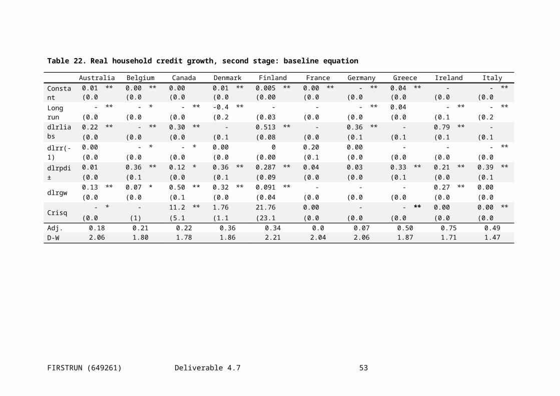
Dell'Ariccia et al. (2012)

Credit booms and busts (dummy)

Macroprudential controls Cross section 175

observationsReduction in probability of a bad boom and a bust


Aikman et al. (2009)

Systemic institutions Capital adequacy Macro stress test using

simulation model10 UK banks at end 2007

Capture feedback effects from liquidity risk and procyclicality. Hence regulatory changes such as capital tightening can affect systemic risks

Gauthier et al. (2012)

Canadian banks Capital requirements Macro stress test using

simulation model

Captures interbank spillover effects; macroprudential capital requirements reduce probabilities of crises and of individual bank failures by around 25 per cent.

Antipa et al. (2010)

US economy Policy rate

DSGE model; modified Taylor rule where the short rate responds to credit growth as well as inflation and authorities can influence the short term credit spread

Policy could have mitigated the last credit cycle and the succeeding recession.

Catte et al. (2010)

US economy Spreads on mortgages NiGEM simulations 2002-7 Mitigation of crisis

Barrell et al. (2010)

OECD countries

Capital and liquidity regulations Macro simulations 1980-2007

Estimates of the degree of macroprudential regulatory tightening needed to reduce crisis probabilities in the subprime crisis, as well as a prediction tool


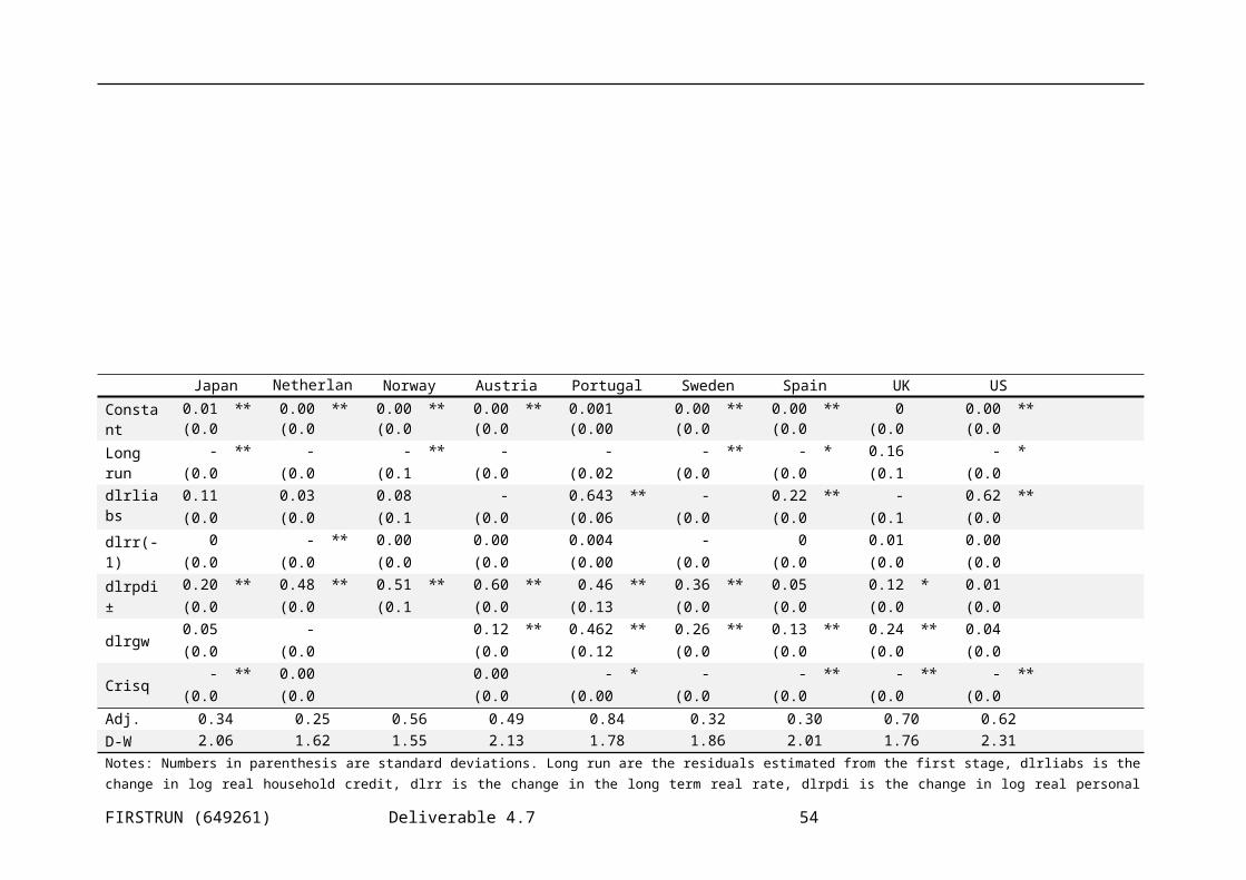
Igan and Kang (2012)

Micro data on mortgage lending in Korea

LTV and DTI limits Micro panel regression 2002-2010 Macroprudential policies have beneficial effect on mortgage credit growth in Korea


Davis, Fic and Karim (2011)

Sweden LTV, capital adequacy on housing NiGEM simulations Simulation

Distinctive effect of macroprudential policies on the economy, more focused than monetary policy or generalised increases in capital adequacy

Aiyar, Calomiris, and Wieladek (2013)

Individual UK banks

Bank-specific higher capital adequacy requirements

Micro panel regression 1998-2007

Capital requirements dampened lending by individual banks but were ineffective due to increased lending from foreign bank branches.


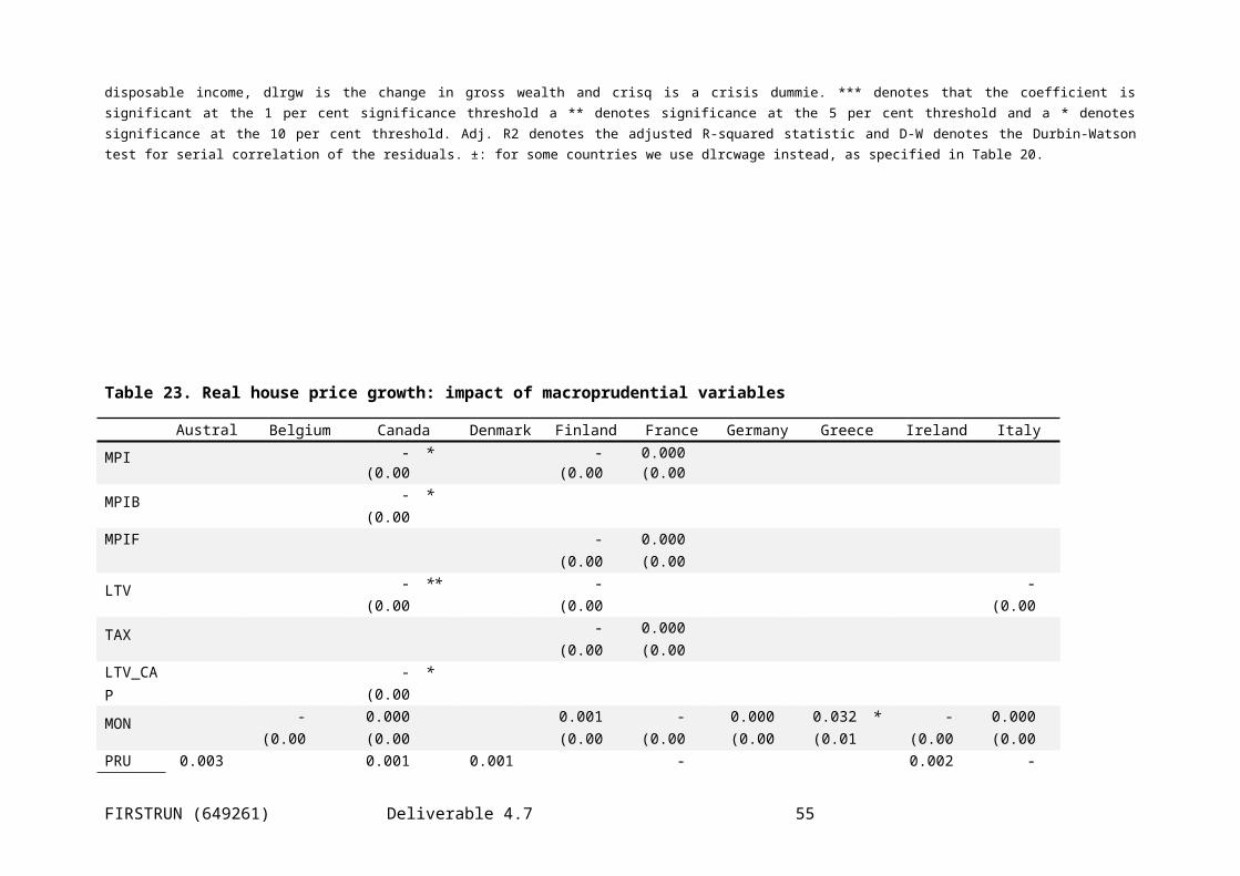
Claessens et al. (2014)

Individual global banks' balance sheets

Policies aimed at borrowers (DTI, LTV), banks' assets or liabilities (CG, FC, RR,), policies that encourage counter-cyclical buffers (CTC, DP) and profits distribution restrictions (PRD)) and miscellaneous policies

Panel GMM

2000-2010, 48 countries, 25 advanced and 23 EMEs, with 2820 banks and 18000 observations.

Policies aimed at borrowers are effective in (indirectly) reducing the build-up of banking system vulnerabilities. Measures aimed at banks' assets and liabilities are very effective, but counter-cyclical buffers do not. The category other is also very effective


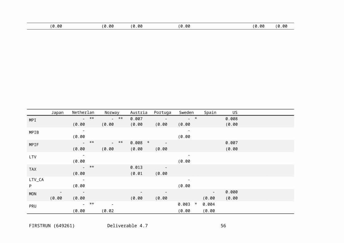
10 Appendix C: estimation of equations for spreadsIn this appendix we show results for spreads equations comparable to those for house prices and household debt. The baseline equation shows that in the long run, the spread widens with RPDI and real long rates but narrows with real gross financial wealth. In the short run there is a significant autoregression, partly offset when the real long rate rises.

Table 26. Baseline equations (2000Q1-2013Q3)

Variable Change in household spread (DLENDW)

C 0.274(0.4)

DLRPDI

DLRR -0.083***(4.1)

DLRPH(-1)

DLENDW(-1) 0.157***(16.6)

LRPDI(-1) 0.278**(2.2)

LRR(-1) 0.015*(1.9)

LRGW(-1) -0.219***(3.5)

CRISES 0.049***(2.8)

R2 0.357SE 0.2OBS 749COUNTRIES 15

Effects on the spread with the IMF variables is confined to the tax variable, a tax on banks widens the spread. The generic BIS PRU variable widens the spread in both data periods, while non-interest monetary action MON narrows it. These results are more strongly borne out for the European countries.


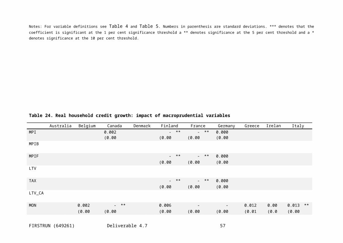
Table 27. Results with first IMF and BIS datasets using baseline equations


MPI 0.015(0.8)

MPIB -0.016(0.3)

MPIF 0.019(0.9)

LTV -0.0077(0.3)

DTI 0.019(0.9)

FC -0.0001(0.1)

TAX 0.065*(1.8)

INTER -0.02(0.5)

CONC 0.26(1.2)

LTV_CAP -0.043(0.6)

MON 0.013(0.4)

PRU 0.037**(2.5)

MON (estimated from 1990) -0.032**(2.2)

PRU (estimated from 1990) 0.036**(2.5)


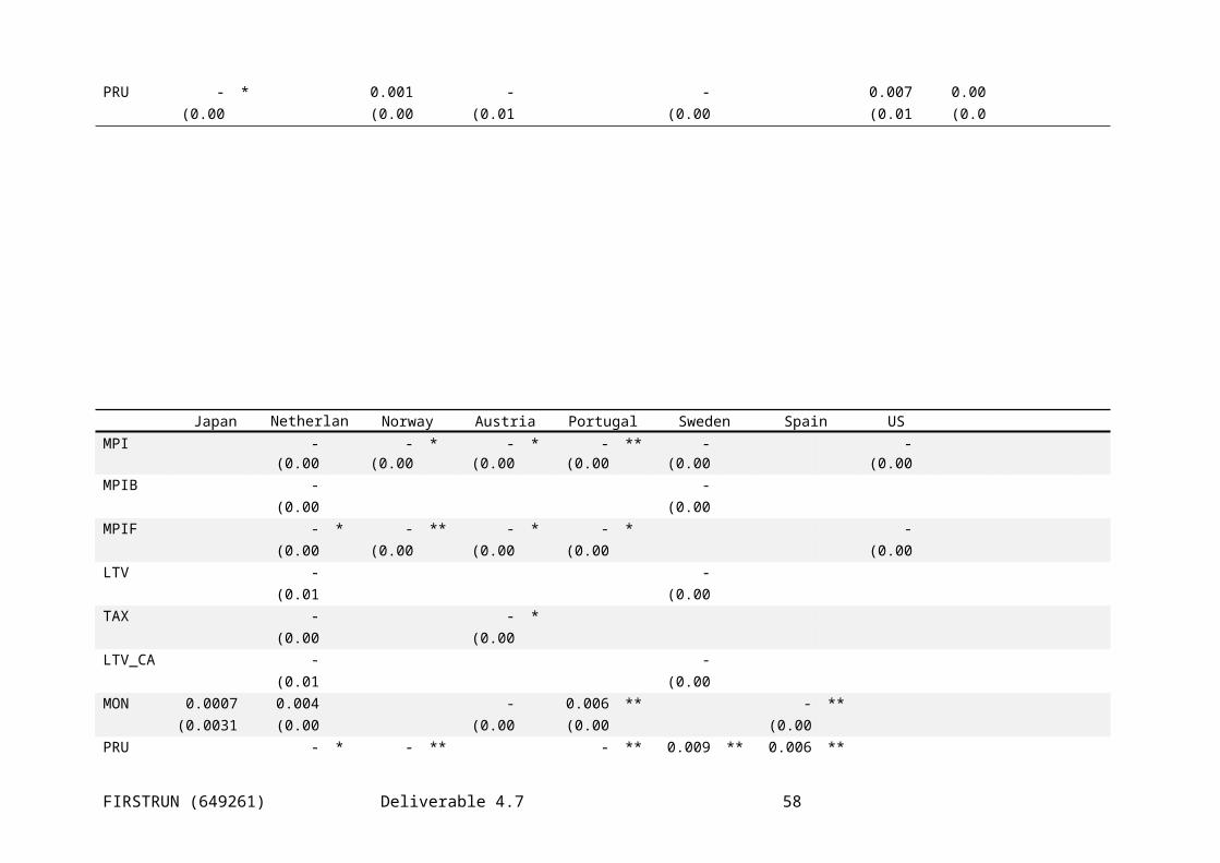
Table 28. Results with first IMF and BIS datasets using baseline equations (Europe only)


MPI 0.014(0.8)

MPIB -0.015(0.3)

MPIF 0.017(0.9)

LTV -0.007(0.3)

FC 0.0015(0.1)

TAX 0.067**(1.9)

INTER -0.02(0.5)

LTV_CAP -0.045(0.6)

MON 0.016(0.5)

PRU 0.036**(2.5)

MON (estimated from 1990) -0.036**(2.4)

PRU (estimated from 1990) 0.039**(2.7)


Documents

Introductionbura.brunel.ac.uk/bitstream/2438/13842/1/Fulltext.docx · Web viewFIRSTRUN – Fiscal Rules and Strategies under Externalities and Uncertainties. Funded by the Horizon