Public Interest Energy Research (PIER) ProgramFINAL PROJECT REPORT

Ocean Wave Climate Change and Associated Implications for Coastal Erosion Along the Southern California CoastPrepared for: California Energy Commission

Prepared by: Peter N. Adams, Douglas L. Inman, Nicholas E. Graham, Jessica L. Lovering, Adam Young, Shaun Kline

1

Acknowledgments

This report was made possible through the financial support of the California Energy Commission’s Public Interest Energy Research (PIER) Program. We gratefully acknowledge Guido Franco, Dan Cayan, Susi Moser, and Myoung-Ae Jones for their assistance and guidance throughout the duration of this project. Our collaboration with Linwood Pendleton, Philip King, Craig Mohn, D. G. Webster, and Ryan K. Vaughn on the assessment of potential economic impacts of climate change on Southern California beaches was very helpful in guiding this research. We are grateful to Bill O’Reilly, Ron Flick, and Bob Guza for their efforts on sea cliff erosion portion of this report. We thank Manu Sethi and Joseph Lovering for their help organizing much of the computer code used in numerical model development and data organization. Pat Masters provided valuable editorial comments. We thank Kraig Winters for his assistance with numerical modeling procedures, and the WHOI/USGS Joint Research groups for SWAN instruction.

Acknowledgements (from Adams Et Al., 2011 Climatic Change Ms)

This manuscript benefitted from thoughtful comments of three anonymous reviewers as well as conversations with Shaun Kline.  This research was funded by the California Energy Commission's (CEC) Public Interest Energy Research Program.  Special thanks are due to Guido Franco at the CEC, and the other guest editors of this special issue.

Acknowledgements (from Young Et Al., 2011 JGR Ms)

Wave data collection was sponsored by the California Department of Boating and Waterways, and the U.S. Army Corps of Engineers, as part of the Coastal Data Information Program (CDIP). APY received Post-Doctoral Scholar support from the California Department of Boating and Waterways Oceanography Program. The California Energy Commission PIER program provided funding for this research. We thank the Del Mar Beach Club, the Solana Beach Lifeguards, and the Jacobs family for their assistance.

2

Preface

3

Table of Contents

1. Introduction1.1. Background on Coastal Evolution Modeling1.2. Regional Setting: Southern California Bight

1.2.1. Geologic Setting1.2.2. Sedimentary Sources1.2.3. Littoral Cells1.2.4. Regional Wave Climate1.2.5. Sea Level History and Projections

2. Southern California Deep-Water Wave Climate Characterization2.1 Section Summary2.2 Section Introduction2.3 Historic Southern California Wave Climate2.4 ENSO and PDO2.5 Wave Climate Hindcast Record2.6 Statistical Analysis

2.6.1 Trend Analysis2.6.2 Population Distributions

2.7 Coastal Wave Energy Flux2.8 Section Conclusions

3.0 Effects of Climate Change on Longshore Sediment Transport Patterns in Southern California

Methods2.1. Model Overview and General Architecture2.2. Model Inputs2.2.1. Bathymetric Data2.2.2. Offshore Wave Climate2.3. Wave Transformation Modeling2.3.1. Lookup Table Development2.3.2. Wave Input Snapping2.3.3. Far Field Grid Wave Field Computation (Coarse Resolution)2.3.4. Near-field Grid Wave Field Computation (Fine Resolution)2.4. Longshore Sediment Transport Modeling2.4.1. Choosing the 5-meter Isobath2.4.2. Decimating Along the 5-meter Isobath2.4.3. Computing Coastal Trends2.4.4. Retrieving and Interpolating SWAN Output2.4.5. Calculating Angle of Incidence2.4.6. Calculating Wave Energy Flux2.4.7. Calculating Divergence of Drift2.5. Model Limitations

4

3.0 Numerical Experiments and Results3.1. Wave Direction Experiment3.1.1. Experimental Design3.1.2. Results3.1.3. Experimental Conclusions and Implications3.2. Erosional Hotspot Likelihood Experiment3.2.1. Experimental Design3.2.2. Results3.2.3. Experimental Conclusions and Implications3.3. Estimating Sea Cliff Retreat from Sea Level Rise3.3.1. Background for Calculations3.3.2. Estimates of the Effects of Sea Level Rise4.0 References

List of Figures

List of Tables

5

Abstract

Global climate change affects sea level elevation and ocean wave patterns. A significant fraction of Southern California’s population is distributed within several tens of miles from the Pacific Ocean coast. The infrastructure supporting this population will be affected by sea level rise and changes in wave energy delivery. This report presents the results of project investigating the potential effects of climate change on the physical environment of the Southern California Pacific Ocean coast. The report is organized into four sections:

1. A background section that provides information on the interconnectedness of components within the physical setting, including the geology, sedimentary sources, littoral cells, wave climate, and sea level history,

2. A study of recent trends in the deep-water wave climate adjacent to the Southern California coast and a characterization of the expected wave climate for specific conditions of global atmospheric climate (El Niño and the Pacific Decadal Oscillation, specifically),

3. A numerical modeling investigation of potential (sedimentary) coastal erosion and accretion for two sites within the Southern California bight, and an interpretation of the results in light of the aforementioned wave climate analysis,

4. A field and modeling study of the mechanics of sea cliff retreat influenced by wave processes, specifically: (1) wave-induced loading fatigue of sea cliff bedrock, and (2) abrasion-driven landsliding of cantilevered cliffs.

The results of the project indicate that due to the geologic, oceanographic, and atmospheric setting of Southern California, climate change-driven wave field alterations will have a significant effect on the distribution of sediment along the coast and the retreat of sea cliffs. In particular, the westerly wave field associated with increased intensity of El Niño storms during the warm phase of the Pacific Decadal Oscillation delivers a greater fraction of deep-water wave energy flux to the coast. These conditions are more effective at: (1) entraining and transporting sediment away from pocket beaches, (2) abrading basal notches in sea cliffs, when only a small quantity of beach sediment is present, and (3) fatiguing cliffs through cyclical wave-induced flexure. Unless accompanied by significant increases in steady terrestrial precipitation, which can provide an ample terrigenous sediment source to the coast, future El Niño wave events will remove large quantities of beach sediment to expose bedrock sea cliffs, leaving a heightened vulnerability for cliff retreat via mechanisms of abrasion, fatigue, and cantilevered block failure.

Keywords: Coastal erosion, wave climate, Southern California, sea level rise, numerical modeling.

6

Executive Summary

Background

Southern California Deep-Water Wave Climate Characterization

Effects of Climate Change on Longshore Sediment Transport Patterns

Sea Cliff Retreat Resulting from Sea Level Rise and Wave Climate Change

7

1. Background

Climate change poses a significant challenge to the future of California’s coast. Nearly 80% of the population of the state of California inhabits the narrow swath of land within 30 miles of the coast (Griggs et al. 2005). Attendant with this population distribution is the infrastructure necessary to support society, including interstate highways, electrical power generation plants, and various commerce facilities. Given the overwhelming evidence that global climate change is upon us and the recognition that eustatic sea level rise is a fundamental result of climate change, it is imperative to assess the oceanographic and geomorphic changes expected within the coastal zone, to mitigate the effects of climate change on coastal communities. Effective planning for the future of the California coast will need to draw on climate models that predict the forcing scenarios and coastal change models that predict the coast’s response.

Evaluating the causes and consequences of coastal change requires an understanding of the processes involved in coastal evolution. Waves, currents, and sediment supply are the primary controls on coastal evolution; any changes in global climate which alter the timing and magnitude of storms and/or raise global sea level will have severe consequences for beaches, coastlines, and coastal structures.

We may organize the effects of climate change on the California coastal zone into the four main categories:

1. Sea level rise and the associated landward migration of the shoreline (inundation), along the cliffed and the sandy beach portions of the coast.

2. Potential changes in littoral sediment budgets caused by a redistribution of nearshore wave energy resulting from sea level rise alone.

3. Potential changes in littoral sediment budgets caused by changes in deep-water storm patterns and intensity, resulting from warming of the ocean-atmosphere system (the main focus of this paper).

4. Potential changes to sediment supply to the littoral system from river discharge.

In this paper, we present a detailed numerical model, which calculates the locations and magnitudes of hotspots of coastal erosion as a function of changes in deep water wave fields that might accompany climate change. We then use the model to conduct a series of numerical experiments to illustrate the model’s utility in addressing questions of climate change and coastal evolution. The numerical experiments chosen address the following questions:

How do changes in deep water wave direction, a likely result of climate change, affect the pattern of erosional hotspot distribution along exposed and sheltered portions of the Southern California Bight? (Section 3.1)

8

What is the variability of potential divergence of longshore drift over a complete cycle of the Pacific Decadal Oscillation, including the effects of severe El Niño winter storms? (Section 3.2)

How will a 1-meter rise in eustatic sea level translate into sea cliff retreat at a relatively stable reach of the Southern California Bight? (Section 3.3)

The purpose of this paper is to present a numerical model and framework for exploring the effects of climate change on the Southern California coast, and to illustrate the utility of such a model through the aforementioned numerical experiments. We specifically chose different sites for each of the first two groups of calculations to show that the model was robust over a range of coastal orientations.

1.1 Background on Coastal Evolution Modeling

For many years, numerical models of coastal sedimentary processes were developed only by engineers, in studies that targeted coastal structure emplacement and the subsequent effects on cross-shore beach profiles and longshore patterns of sediment transport. With applications aimed at aiding shipping industry, these models focused on “real-time” processes with time-windows that covered seasonal to annual scales at most (Larson and Kraus 1989).

In the past 20 years, tremendous strides have been made in the field of geomorphic evolution modeling in response to long-term climate variation. Examples from such varied environments as alpine glacial valleys (MacGregor et al. 2000), terraced fluvial plains (Hancock and Anderson 2002), and tectonically active coasts (Anderson et al. 1999) provide hope that we can combine the physical processes of terrestrial sedimentary sources (rivers and sea cliffs) with nearshore oceanographic processes (waves, tides, and currents) to develop an understanding of how sedimentary coasts respond to climatic changes. Within the scope of this study, we focus on relatively short-term geomorphic changes that may occur on the decadal to century time scale.

Most recently, researchers have worked to develop so-called ”one-line” numerical models of coastal evolution, in which the assumption is made that cross-shore profile shape is constant, while shoreline position varies (Pelnard-Considere 1956). Conservation of mass is the fundamental concept employed in one-line models, wherein sediment accumulation (or depletion) within a coastal compartment results from the divergence of littoral drift (i.e., the first spatial derivative of volumetric longshore sediment transport rate). Utilizing a one-line coastal evolution model, Ashton et al. (2001) explored the concept of high-angle waves in the stability of large, coastal planform features. In a recent study by Ruggiero et al. (2006), a one-line coastal evolution model (UNIBEST) was used in conjunction with a wave transformation model (SWAN) to investigate probabilities of decadal shoreline change along the Washington coast. List et al. (2007) have explored predictions of longshore sediment transport gradients with the advanced, process-based Delft3d nearshore flow model.

9

1.2 Regional Setting: Southern California Bight

For the purposes of this study, we consider the Southern California Bight to extend from a northwestern-most boundary at Point Arguello (34.58°, -120.65°, Figure 1-1) to the U.S.-Mexico border (32.54°, -117.12°, Figure 1-1) south of San Diego. Within this region, we have also established several subregions (~10 kilometers [km] to ~100 km reaches) where coastal evolution can be modeled and studied with higher spatial resolution (Figure 1-2). Throughout this paper, we refer to these subregions as “nests,” a term borrowed from the terminology of the wave transformation model, covered in greater detail in Section 2.3. In sections 1.2.1 thru 1.2.5, we describe the geologic setting, sedimentary sources, littoral cells, regional wave climate, and sea level rise history for the Southern California Bight.

1.2.1 Geologic Setting

Tectonic processes are responsible for shaping the shallow ocean basins, continental shelf, and large-scale terrestrial landmasses adjacent to Southern California’s coast. The tectonic setting for Southern California is considered to be a collisional or active margin, which occurs where two plates impinge upon one another (Inman and Nordstrom 1971). On the active transform boundary between the Pacific and North American plates, the leading edge of the plate boundaries have been folded and fractured by transpressional plate motions. In particular, the coastal mountain ranges and local shelf basins have been constructed by crustal displacement and tectonic activity along a network of subparallel strike-slip faults, which characterize the North American plate-Pacific plate interface (Hogarth et al. 2007). In general, these motions have resulted in the highly irregular, complex bathymetry that makes up the California Borderlands (Legg 1991; Shepard and Emery 1941), decorated with the subaerially exposed Channel Islands, as well as numerous submerged seamounts and troughs, shown in Figure 1-3. This collisional margin coast is typified by a narrow, steep continental shelf (~10 km wide), deeply incised submarine canyons, and beaches backed by resistant, bedrock sea cliffs. This coastal geomorphology contrasts with the passive or trailing edge margin of the eastern United States, where sedimentary processes dominate, resulting in a broad subaerial coastal plain and a continental shelf that is wide (~50 km to 100 km) and gently sloping.

1.2.2 Sedimentary Sources

Globally, the sources of sediment to the coastal zone are dominantly fluvial. Where rivers meet the coast in Southern California, there are often local depositional basins (sedimentary deltas), which temporarily store fluvial sediment as it awaits incorporation into longshore sediment in the littoral system. The major rivers responsible for delivering sediment to the Southern California coast are the Santa Maria, the Santa Ynez, the Santa Clara, the Los Angeles, the San Gabriel, the Santa Ana River, the Santa Margarita, the San Luis Rey, and the Tijuana. Each of the aforementioned rivers drain catchments that exceed 1000 square kilometers (km2) in area (Inman and Jenkins 1999). Intermittent streams follow steep-sided canyons as they emerge from the coastal ranges, and all but a few drainages are relatively small with high gradients. It has been shown that rivers draining

10

small, mountainous, coastal catchments provide a surprisingly large fraction of littoral sediment to the nearshore zone (Milliman 1995; Milliman and Syvitski 1992), and that sediment discharge from these rivers can be significantly influenced by climatic variability (Cayan et al. 1999; Farnsworth and Milliman 2003; Warrick and Milliman 2003). With Southern California’s semiarid climate, sediment supply to the coast is limited to runoff events from winter storms, making the beaches sand limited.

1.2.3 Littoral Cells

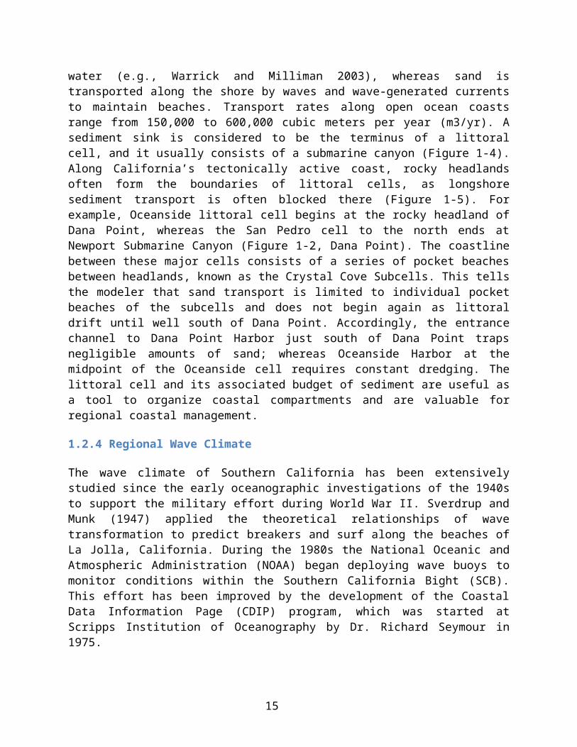
The littoral cell, shown schematically in Figure 1-4, is the coastal compartment that contains the sources, transport paths, and sinks of sediment (Inman 2005; Inman and Frautschy 1965). Sediment sources on cliffed coasts are (1) rivers, which deliver the products of terrestrial erosion, and (2) sea cliffs, which erode and retreat due to attack by waves. Fine suspended sediment is carried offshore in turbid plumes and deposited in deeper water (e.g., Warrick and Milliman 2003), whereas sand is transported along the shore by waves and wave-generated currents to maintain beaches. Transport rates along open ocean coasts range from 150,000 to 600,000 cubic meters per year (m3/yr). A sediment sink is considered to be the terminus of a littoral cell, and it usually consists of a submarine canyon (Figure 1-4). Along California’s tectonically active coast, rocky headlands often form the boundaries of littoral cells, as longshore sediment transport is often blocked there (Figure 1-5). For example, Oceanside littoral cell begins at the rocky headland of Dana Point, whereas the San Pedro cell to the north ends at Newport Submarine Canyon (Figure 1-2, Dana Point). The coastline between these major cells consists of a series of pocket beaches between headlands, known as the Crystal Cove Subcells. This tells the modeler that sand transport is limited to individual pocket beaches of the subcells and does not begin again as littoral drift until well south of Dana Point. Accordingly, the entrance channel to Dana Point Harbor just south of Dana Point traps negligible amounts of sand; whereas Oceanside Harbor at the midpoint of the Oceanside cell requires constant dredging. The littoral cell and its associated budget of sediment are useful as a tool to organize coastal compartments and are valuable for regional coastal management.

1.2.4 Regional Wave Climate

The wave climate of Southern California has been extensively studied since the early oceanographic investigations of the 1940s to support the military effort during World War II. Sverdrup and Munk (1947) applied the theoretical relationships of wave transformation to predict breakers and surf along the beaches of La Jolla, California. During the 1980s the National Oceanic and Atmospheric Administration (NOAA) began deploying wave buoys to monitor conditions within the Southern California Bight (SCB). This effort has been improved by the development of the Coastal Data Information Page (CDIP) program, which was started at Scripps Institution of Oceanography by Dr. Richard Seymour in 1975. The presence of the Channel Islands (Figures 1-1 and 1-3) significantly alters the deep-water (open ocean) wave climate to a more complicated nearshore wave field along the Southern California coast. The islands intercept waves approaching from almost any direction and the shallow water bathymetry adjacent to the islands refracts and reorients

11

wave rays to produce a complicated wave energy distribution along the coast of the Southern California mainland. Several studies have targeted the sheltering effect of the Channel Islands within the SCB and the complexity of modeling wave transformation through such a complicated bathymetry (e.g., O'Reilly 1993; O'Reilly and Guza 1993; Pawka 1983; Rogers et al. 2007). The resulting distribution of wave energy at the coast consists of dramatic longshore variability in wave energy flux and radiation stress. These factors are considered to be fundamental in generating the nearshore currents responsible for longshore sediment transport and the maintenance of sandy beaches.

Recently, Adams et al. (2008) examined a 50-year (1948–1998) numerical hindcast of deep-water, winter wave heights, periods, and directions for location 33˚N/121.5˚W, to understand the correlation of decadal-to-interannual climate variability with offshore wave fields. Their study found that El Niño-type winters during Pacific Decadal Oscillation (PDO) warm phase have significantly more energetic wave fields than those during PDO-cool phase, suggesting an interesting connection between global climate change and coastal evolution, based on patterns of storminess (Figure 1-6).

1.2.5 Sea Level History and Projections

During the Quaternary geologic period, eustatic (global) sea level has experienced wide-ranging fluctuation due in large part to climatic variability (Ruddiman 2002). Since the last glacial maximum (LGM) approximately 18–20 thousand years ago, sea level has been rising from approximately 120 meters below modern level to its present state (Figure 1-7). The details of this transgression indicate that the rate of sea level rise has not been steady. Exceptionally warm periods drive increased rates of melting of glacial ice, which provide a pulse of water to the world’s oceans, causing short-lived intervals of rapid sea level rise. Over the last five thousand years, eustatic sea level has been relatively stable or rising very slowly, save for the recent increase in sea level rise rate, estimated from tide gauge records from San Francisco, to a value of 2.2 millimeters [mm] per year (20 centimeters [cm] per century) over the last several decades (Flick et al. 2003). From a set of climate simulations for a series of different greenhouse gas emissions scenarios, Cayan et al. (2008) calculate a potential sea level rise of up to 72 cm by 2070–2099 (7.9 to 11.6 mm/yr). This estimate indicates a 3.6x to 5.3x increase in sea level rise rate. This current estimate illustrates the need to understand the potential hazards threatening the California coast due to inundation by sea level rise and changes in wave storminess due to sea level rise–induced changes in climatic circulation.

12

2. Southern California Deep-Water Wave Climate Characterization

This section of the report presents our investigation of the recent history of wave climate within the southern California bight. Some of the material contained in this section was prepared for publication in the Journal of Coastal Research in 2008 as the following:

Adams, P. N., Inman, D., & Graham, N. (2008). Southern California deep-water wave climate: Characterization and application to coastal processes. Journal of Coastal Research, 24(4), 1022–1035.

2.1 Section Summary

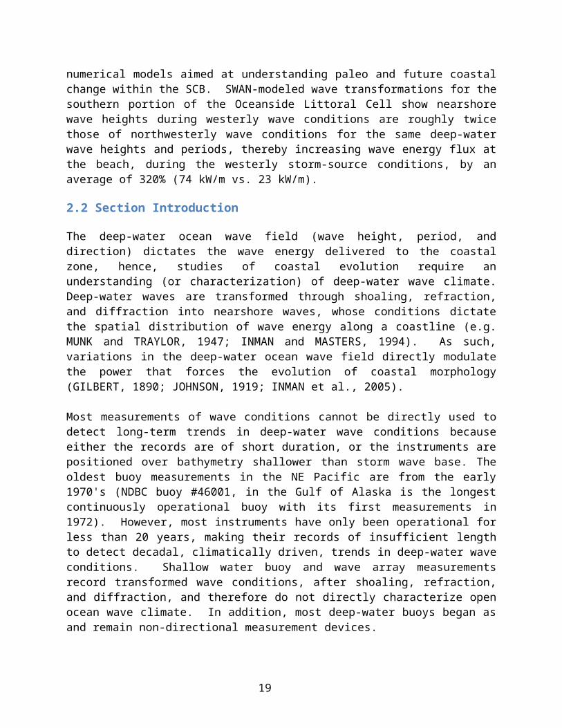
We consider the effect of decadal climate change on the historic wave climate of the Southern California Bight (SCB) using a 50-year hindcast record (1948-1998) for waves generated in the North Pacific winter. Deep-water wave height, period, and direction are examined with respect to the Southern Oscillation Index (SOI) and the Pacific Decadal Oscillation (PDO). Storms occurring during strong La Niña intervals, when the SOI is greater than 1.0, concurrent with either cool- or warm-phase of the PDO are indistinguishable in wave character. In marked contrast, wave conditions arising from storms during strong El Niño intervals, when the SOI is less than -1.0, concurrent with the PDO cool-phase (1948-1977) differ greatly from wave conditions of storms during strong El Niño intervals concurrent with the PDO warm-phase (1978-1998). Our statistical analyses characterize the deep-water winter wave climate as consistent during La Niña intervals (mean values Hs = 3.3 m, Ts = 13.0 s, = 293˚, for the highest 5% of waves), butα variable during El Niño intervals depending on PDO phase (Hs = 3.64 m, Ts = 13.8 s, =α 292˚ during the PDO cool-phase, and Hs = 4.82 m, Ts = 15.1 s, = 284˚ during the PDOα warm-phase, for the highest 5% of waves). The dominant characteristics for the different operational modes of wave climate determined in this study provide realistic inputs for numerical models aimed at understanding paleo and future coastal change within the SCB. SWAN-modeled wave transformations for the southern portion of the Oceanside Littoral Cell show nearshore wave heights during westerly wave conditions are roughly twice those of northwesterly wave conditions for the same deep-water wave heights and periods, thereby increasing wave energy flux at the beach, during the westerly storm-source conditions, by an average of 320% (74 kW/m vs. 23 kW/m).

2.2 Section Introduction

The deep-water ocean wave field (wave height, period, and direction) dictates the wave energy delivered to the coastal zone, hence, studies of coastal evolution require an understanding (or characterization) of deep-water wave climate. Deep-water waves are transformed through shoaling, refraction, and diffraction into nearshore waves, whose conditions dictate the spatial distribution of wave energy along a coastline (e.g. MUNK and TRAYLOR, 1947; INMAN and MASTERS, 1994). As such, variations in the deep-water ocean

13

wave field directly modulate the power that forces the evolution of coastal morphology (GILBERT, 1890; JOHNSON, 1919; INMAN et al., 2005).

Most measurements of wave conditions cannot be directly used to detect long-term trends in deep-water wave conditions because either the records are of short duration, or the instruments are positioned over bathymetry shallower than storm wave base. The oldest buoy measurements in the NE Pacific are from the early 1970's (NDBC buoy #46001, in the Gulf of Alaska is the longest continuously operational buoy with its first measurements in 1972). However, most instruments have only been operational for less than 20 years, making their records of insufficient length to detect decadal, climatically driven, trends in deep-water wave conditions. Shallow water buoy and wave array measurements record transformed wave conditions, after shoaling, refraction, and diffraction, and therefore do not directly characterize open ocean wave climate. In addition, most deep-water buoys began as and remain non-directional measurement devices.

To resolve this paucity in data, numerical models of ocean-atmosphere interaction have been developed to simulate wave conditions over the open ocean, given a known wind field (TOLMAN, 1999). Hindcasts from these models, have been verified through comparison to measured conditions (GRAHAM and DIAZ, 2001; WANG and SWAIL, 2001; CAIRES et al., 2004; GRAHAM, 2005). These studies show that although various wave hindcasts have a range of biases and uncertainties arising from both wave model limitiations and the wind data used to drive them, they are very useful for examining both long-term trends and particular events.

The causes and character of inter-decadal to interannual climate variability over the Pacific sector has been studied closely over the past few decades (BJERKNES, 1969; LAU, 1985; MANTUA et al., 1997). El Niño-Southern Oscillation (ENSO) tends to vary on a timescale of 2 – 7 years, and has particularly strong effects on the intensity of the winter circulation over the North Pacific. These changes tend to result in stronger storms taking more southerly tracks over the Northeast Pacific during strong El Niño years making the Southern California coast particularly sensitive to ENSO state (SEYMOUR et al., 1984; INMAN et al., 1996; SEYMOUR, 1998; GRAHAM, 2005). Wave climate, precipitation, and riverine sediment flux are strongly influenced by El Niño events (SEYMOUR et al., 1984; CAYAN et al., 1999; INMAN and JENKINS, 1999; STORLAZZI and GRIGGS, 2000; ANDREWS et al., 2004; GRAHAM, 2005; PINTER and VESTAL, 2005), and determine the supply of sediment to beaches – a variable of fundamental importance in coastal evolution. The decadal to interdecadal variability in North Pacific winter circulation also influences the Southern California climate (GRAHAM and DIAZ, 2001; GRAHAM, 2005; ALLAN and KOMAR, 2006; KNOWLES et al., 2006), which is quantified by the Pacific Decadal Oscillation (PDO) index (MANTUA et al., 1997; MANTUA and HARE, 2002).

Several teams of researchers have drawn attention to a decadal trend of increased storm intensity, wave height, and wave period affecting the U.S. Pacific coast, extending from Washington to south-central California, during the past ~25 years (early 1980's to present), that may be linked to climate change and ENSO variability (GRAHAM and DIAZ, 2001; WANG and SWAIL, 2001; ALLAN and KOMAR, 2006). They report a latitudinal

14

dependence of the magnitudes of (i) wave height and (ii) wave runup level that increase from Pt. Arguello, California to the coast of Washington. Similar results were found by STORLAZZI and WINGFIELD (2005) in their analysis of data from eight deep-water buoys during 1980-2002. BROMIRSKI et al. (2003) showed that for the central California coast, extreme winter non-tidal residual levels have been increasing since 1950, and correlate temporally to sea level pressure anomalies that are thought to be related to changes in winter storm strength and track in the northeast Pacific. In contrast, XU and NOBLE (2007) compared wind and wave data from deep-water and nearshore buoys within the Southern California Bight (SCB), and found negligible temporal trend in the data.

The SCB was selected for this study because it has a long historical record of waves and includes highly populated areas where knowledge of wave forcing is essential to the present and future of coasts and beaches. Wave hindcast and forecast procedures were first developed here by SVERDRUP and MUNK (1947) for World War II amphibious landings (e. g. INMAN, 2003). The application of wave energy flux to the nearshore areas of the SCB soon followed, including the first wave climate in the form of tables of hindcast waves for stations along the California coast (ARTHUR et al., 1947). As a consequence, an unusually long historical record of waves and associated beach response is available for the SCB as discussed below.

2.3 Historic Southern California Wave Climate

Wave climate can be defined as the set of prevailing wave conditions within a particular oceanic or coastal region over a defined time interval (INMAN and MASTERS, 1994). Most of the wave energy for the SCB is generated by mid-latitude winter cyclones (storms) in the North Pacific. Other important sources of wave energy include (a) waves generated by the prevailing northwesterly winds along the California coast during spring and summer, and (b) swells from winter storms in the Southern Hemisphere mid-latitudes which are common, though generally delivering small waves. Eastern Pacific tropical storms occasionally produce large waves in the offshore Southern California region as do local wind episodes (generally from the northwest or southeast) usually associated with passing or approaching low pressure centers (MUNK and TRAYLOR, 1947; HORRER, 1950; SEYMOUR et al., 1984; STRANGE et al., 1989; O'REILLY, 1993; INMAN et al., 1996; SEYMOUR, 1996; FLICK, 1998; SEYMOUR, 1998; STORLAZZI et al., 2000).

As a convenient, though not rigorous, way to think about the SCB wave climate, we describe six characteristic "wave types" assembled from various data sources (Figure 1 and Table 1). The concept of characteristic "wave types" associated with wave generation source and intensity was introduced by MUNK and TRAYLOR (1947) and ARTHUR et al. (1947). The six characteristic "wave types" shown in Figure 1 are based on their original concept of generation area with central values and likely ranges of open ocean wave height, period, and direction (Table 1). Here we have updated this schematic to include the more recent understanding of wave climate, particularly the occurrence of decadal ENSO cycles (e.g. MCPHADEN et al., 2006), and the extensive historic record of hindcast computations and measurements of various kinds.

15

The historic record for the SCB includes five hindcast studies of the North Pacific Ocean ranging from three years (1936 – 38) to the recent 50-year (1948 – 98) data set, analyzed herein (e.g. ARTHUR et al., 1947; NATIONAL_MARINE_CONSULTANTS, 1960; MARINE_ADVISERS, 1961; METEOROLOGY_INTERNATIONAL_INC., 1977; GRAHAM and DIAZ, 2001). In addition, NOAA buoys in the eastern North Pacific have provided continuous wave measurements during the past 30 years (e.g. INMAN and JENKINS, 2005a; ALLAN and KOMAR, 2006). Also, nearshore wave measurements range from systematic visual estimates along beaches (e.g. SHEPARD and INMAN, 1951) to energy-frequency spectra from nearshore wave arrays (e.g. PAWKA et al., 1976) and a multi-station long-term series of measurements in the SCB known as the Coastal Data Information Program (CDIP) (SEYMOUR et al., 1985). References most applicable to the six characteristic "wave types" are listed in the footnotes in Table 1.

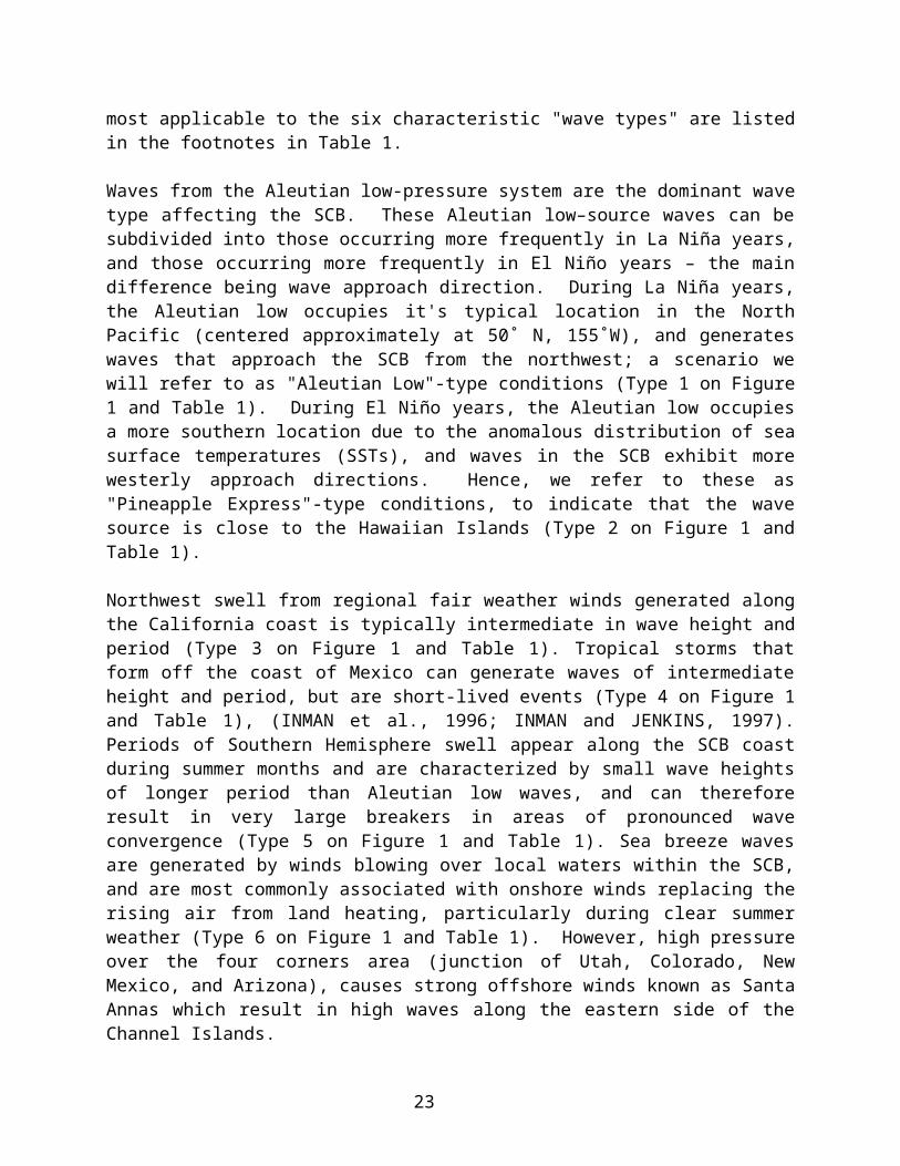
Waves from the Aleutian low-pressure system are the dominant wave type affecting the SCB. These Aleutian low–source waves can be subdivided into those occurring more frequently in La Niña years, and those occurring more frequently in El Niño years – the main difference being wave approach direction. During La Niña years, the Aleutian low occupies it's typical location in the North Pacific (centered approximately at 50˚ N, 155˚W), and generates waves that approach the SCB from the northwest; a scenario we will refer to as "Aleutian Low"-type conditions (Type 1 on Figure 1 and Table 1). During El Niño years, the Aleutian low occupies a more southern location due to the anomalous distribution of sea surface temperatures (SSTs), and waves in the SCB exhibit more westerly approach directions. Hence, we refer to these as "Pineapple Express"-type conditions, to indicate that the wave source is close to the Hawaiian Islands (Type 2 on Figure 1 and Table 1).

Northwest swell from regional fair weather winds generated along the California coast is typically intermediate in wave height and period (Type 3 on Figure 1 and Table 1). Tropical storms that form off the coast of Mexico can generate waves of intermediate height and period, but are short-lived events (Type 4 on Figure 1 and Table 1), (INMAN et al., 1996; INMAN and JENKINS, 1997). Periods of Southern Hemisphere swell appear along the SCB coast during summer months and are characterized by small wave heights of longer period than Aleutian low waves, and can therefore result in very large breakers in areas of pronounced wave convergence (Type 5 on Figure 1 and Table 1). Sea breeze waves are generated by winds blowing over local waters within the SCB, and are most commonly associated with onshore winds replacing the rising air from land heating, particularly during clear summer weather (Type 6 on Figure 1 and Table 1). However, high pressure over the four corners area (junction of Utah, Colorado, New Mexico, and Arizona), causes strong offshore winds known as Santa Annas which result in high waves along the eastern side of the Channel Islands.

The effect of sheltering on frequency-directional spectra has been studied in detail from wave-directional arrays off Torrey Pines Beach in the SCB, and in comparison with synthetic aperture radar (SAR) mounted on aircraft (PAWKA et al., 1976; PAWKA et al., 1980; PAWKA, 1983; PAWKA et al., 1983, 1984). Two examples of sheltering effects include Point Conception, at the northern end of the SCB, which blocks waves that approach from directions north of 315˚, and San Clemente Island, which causes a deep

16

trough in the directional spectrum at Torrey Pines Beach, with a northern peak associated with the window between San Clemente and San Miguel-Santa Rosa Islands, and a southern peak due to wave refraction over Cortez and Tanner Banks. In general, the SCB coastal/island geometry can be described by three fundamental factors: (i) the regional trend of the coastline within the SCB is NW-SE, (ii) Point Conception blocks northwesterly waves, and (iii) the Channel Islands and complex bathymetry of the California Borderlands complicate swell patterns through refraction, diffraction, and sheltering. These factors favor waves with westerly approaches to deliver the bulk of coastal wave energy. We note, however, that because of the aforementioned complexities of SCB bathymetry, the precise spatial distribution of wave energy along the SCB coast is highly dependant on deep-water wave direction.

2.4 ENSO and PDO

The coupled ocean-atmosphere instability known as the El Niño Southern Oscillation (ENSO) produces El Niño episodes when SSTs in the eastern and central equatorial Pacific Ocean warm above the climatological mean by 1-3 ˚C (with respect to seasonal averages). Such episodes tend to reoccur on time scales of 2 – 7 years. The changes in sea surface temperatures (SSTs) alter patterns of convective precipitation in the tropical Pacific, which in turn causes changes in the winter circulation patterns over the North Pacific, resulting in a tendency for stronger storms to track farther south and east than usual (BJERKNES, 1969; LAU, 1985).

Not surprisingly, there is a general tendency for larger waves from westerly approaches to affect Southern California waters in El Niño years – a tendency that is particularly apparent during strong El Niño episodes, when eastern tropical Pacific SSTs are much warmer than normal, as occurred during the winters of 1982-83 and 1997-98 (GRAHAM, 2003). During El Niño years, it is common to see a negative sea level pressure anomaly in the North Pacific centered at approximately 40˚N, 160˚W, which has the effect of shifting storm tracks to the south and east, strengthening wave activity within the SCB. Additionally, there is a tendency for increased precipitation in Southern California during strong El Niño years (particularly noticeable during individual strong El Niño events), a factor which alters typical patterns of riverine sediment delivery to the littoral system (CAYAN et al., 1999; INMAN and JENKINS, 1999).

In contrast to El Niño episodes, La Niña episodes are periods when SSTs in the eastern tropical Pacific are well below average. Such episodes tend to occur during some years between El Niño episodes, and drive an atmospheric response that is roughly opposite, yet somewhat less systematic, to that observed during El Niño episodes (HOERLING and TING, 1994). During La Niña years, the storm track tends to shift northward, and does not extend to the east over the sub-tropical latitudes of the Northeast Pacific. Although storm intensity may be high during La Niña years, the northwesterly wave approach is blocked by the coastal salient at Point Conception, which provides protection to the SCB coast from large wave attack.

17

El Niño activity can be quantified by several different indicies, based on temperature or atmospheric pressure anomalies in the equatorial Pacific. One widely used index is the NINO3 SST index which is the area-averaged SST anomaly over the region from 150˚W – 90˚W longitude and 5˚N – 5˚S latitude (see KAPLAN et al. (1998) for a reconstruction of equatorial SSTs). In this paper we use the Southern Oscillation index (SOI), the historically longest index (WALKER, 1928), computed as the normalized sea level pressure difference between Tahiti and Darwin, Australia (Figure 2a).

Climatic variability observed in the North Pacific has been referred to as the Pacific Decadal Oscillation (PDO, Figure 2b) or Pacific Decadal Variability (MANTUA et al., 1997). The PDO refers to the observed low-frequency variability (on the order of 20-50 years) in the strength of winter circulation over the North Pacific. The characteristic pattern of changes (or tendencies) with winter North Pacific circulation associated with PDO are essentially the same as those associated with El Niño / La Niña variability. Over the past century, it is clear that PDO variability mimics a smoothed expression of changes in the frequency and intensity of El Niño / La Niña episodes.

PDO is a useful index of changes in the intensity of the winter circulation over the North Pacific, and thus the tendencies for changes in winter cyclone tracks and strength. The original (and most frequently used) measure of PDO is the time series of SSTs averaged over the central North Pacific (as expressed by their first principal component). This PDO index provides a natural proxy for integrated storm activity over the North Pacific, as there is a strong correlation between PDO and winter wave climate indices in the North Pacific (MANTUA et al., 1997). Positive values of the PDO index (PDO warm phase) reflect periods when North Pacific sea surface temperature anomalies are positive. When winter cyclones are strong, frequent, and relatively south of their normal track during the PDO warm-phase in the Eastern Pacific, they produce cool SSTs over the central Pacific Ocean and produce large waves with approach directions favorable to deliver more wave energy to the SCB than usual. When winter cyclones are weaker, less frequent, and tracking further north, SSTs are warmer and swells delivered to the SCB tend to be smaller with more northwesterly approach directions. In this paper, we use the SST-based PDO index as originally defined by MANTUA et al. (1997), (Figure 2b).

The wind fields responsible for wave generation in the North Pacific have a characteristic variability that correlates with PDO phase. During periods of PDO warm-phase (when PDO index is positive), mid-latitude wind fields generally witness a westerly intensification, in accordance with observed mean sea level pressure changes (Graham and Diaz, 2001). El Niño intervals exhibit similar wind fields to those of the PDO warm phase, though the individual storm events are generally short-lived (several days or less).

2.5 Wave Climate Hindcast Record

In what follows, we investigate the correlations between ENSO/PDO and regional wave climate in the SCB (Figure 3), by applying simple statistical procedures to the results from a numerical hindcast of deep-water winter wave conditions. In doing so, we reprise elements of previous work (GRAHAM, 2005), adding some new analyses and providing

18

results from a high-resolution regional wave model. We attempt to address two principal questions: (1) What are the characteristic wave conditions in deep water off Southern California produced during various ENSO and PDO climatic states? (2) How do changes in ENSO and PDO climatic states correlate to deep-water and nearshore wave climate of the SCB?

The wave data set used in this study comes from the numerical hindcast for the 50-year period 1948-1998 described in GRAHAM and DIAZ (2001) and GRAHAM (2003). The wind forcing for the wave data comes from the NCEP-NCAR reanalysis project (KALNAY et al., 1996; KISTLER et al., 2001). This data set represents the last full cycle of decadal climate change (full PDO cycle, Figure 2b). The hindcast domain is the North Pacific Ocean (20°N - 60°N, 150°W - 110°W) with a spatial resolution of 1˚ latitude x 1.5˚ longitude. Data were produced for winter months (DJFM), with 3 hourly spectra recorded in 20 frequency bins (covering the wave period range of ~ 4.5 s – 26 s), and 5 degree directional resolution grouped in 72 bins. The summary outputs used in this paper, calculated from wave energy in the spectral bins, are (1) significant wave height (Hs) in deep water, (2) peak (spectrally-dominant) wave period of the significant wave height (Ts), and (3) peak (spectrally-dominant) wave direction ( ), for the reference deep-water location 33°N, 121.5°Wα (Figure 3); a hindcast node in the model domain. This location was chosen for its position west (oceanward) of the Channel Islands in the SCB. This location has the advantage of representing an open ocean wave climate signal, not subject to island sheltering, shoaling, and the complex refraction and diffraction patterns within the SCB, discussed by PAWKA (1983), PAWKA et al. (1984), and O'REILLY and GUZA (1993).

GRAHAM (2005) made a comparison of the 50-year hindcast record with measurements, where available, from NOAA buoys. Generally, good agreement was found although there was a slight low bias off Southern California for hindcast wave heights from the northwest associated with (i) underestimates of northwesterly coastal winds in the NCEP-NCAR reanalysis, and (ii) coarse resolution of coastal geometry. Treating the 50-year hindcast record as a time series, GRAHAM (2005) used empirical orthogonal functions to show that wave height and wave energy incident to the coast increase over the 50-year period.

2.6 Statistical Analysis

2.6.1 Trend Analysis

Temporal trends in the wave height, period, and direction time series are difficult to detect by simple inspection (e.g. Figure 4a). Following the work of HURST (1951), we use a cumulative residual analysis to find intervals in the time series that depart significantly from mean values. In a cumulative residual analysis, the mean of the time series is subtracted from each observation to obtain a time series of residuals (departures from the mean). The residuals are then cumulatively summed and plotted as a separate time series. Positive slopes on a cumulative residual time series indicate intervals where the variable of interest is consistently above the mean value and negative slopes correspond to intervals below the mean (e.g. Figure 4b).

19

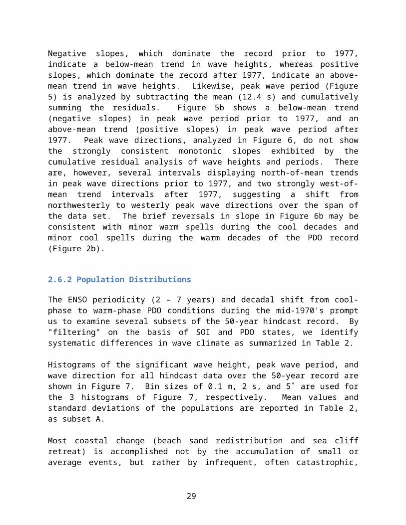
Significant wave heights are plotted as mean monthly values and mean annual values in Figure 4a. The residuals, computed by subtracting the mean (1.67 m) from the data set, are cumulatively summed to obtain the cumulative residual plot shown in Figure 4b for mean monthly and mean annual significant wave height. Negative slopes, which dominate the record prior to 1977, indicate a below-mean trend in wave heights, whereas positive slopes, which dominate the record after 1977, indicate an above-mean trend in wave heights. Likewise, peak wave period (Figure 5) is analyzed by subtracting the mean (12.4 s) and cumulatively summing the residuals. Figure 5b shows a below-mean trend (negative slopes) in peak wave period prior to 1977, and an above-mean trend (positive slopes) in peak wave period after 1977. Peak wave directions, analyzed in Figure 6, do not show the strongly consistent monotonic slopes exhibited by the cumulative residual analysis of wave heights and periods. There are, however, several intervals displaying north-of-mean trends in peak wave directions prior to 1977, and two strongly west-of-mean trend intervals after 1977, suggesting a shift from northwesterly to westerly peak wave directions over the span of the data set. The brief reversals in slope in Figure 6b may be consistent with minor warm spells during the cool decades and minor cool spells during the warm decades of the PDO record (Figure 2b).

2.6.2 Population Distributions

The ENSO periodicity (2 – 7 years) and decadal shift from cool-phase to warm-phase PDO conditions during the mid-1970's prompt us to examine several subsets of the 50-year hindcast record. By "filtering" on the basis of SOI and PDO states, we identify systematic differences in wave climate as summarized in Table 2.

Histograms of the significant wave height, peak wave period, and wave direction for all hindcast data over the 50-year record are shown in Figure 7. Bin sizes of 0.1 m, 2 s, and 5˚ are used for the 3 histograms of Figure 7, respectively. Mean values and standard deviations of the populations are reported in Table 2, as subset A.

Most coastal change (beach sand redistribution and sea cliff retreat) is accomplished not by the accumulation of small or average events, but rather by infrequent, often catastrophic, extreme events. Because wave energy flux governs most coastal processes and energy flux is proportional to the square of the wave height, we chose to analyze the characteristics of the highest 5% (95th percentile and above) of waves in the numerical hindcast data set. We find that the highest 5% of waves account for 23% of the total wave energy in the hindcast record, thereby making it a useful statistic in determining the characteristics of waves of geomorphic consequence. Histograms of significant wave height, peak wave period, and peak wave direction of the highest 5% of waves in the 50-year hindcast data set are shown in Figure 8, with mean values and standard deviations of the populations reported in Table 2, as subset B.

As expected, the population of highest 5% of waves (Table 2, subset B and Figure 8) is markedly different in its mean characteristics as compared to the entire population of hindcast data. Mean significant wave height is more than double that of the entire

20

population (Hs,5% = 3.98 m vs. Hs,all = 1.68 m), mean peak wave period is greater by 14% (Ts,5% = 14.1 s vs. Ts,all = 12.4 s), and wave direction is more westerly by 7˚ ( 5% = 289˚α vs. all = 296˚), reflecting the importance of El Niño storm waves in the highest 5% record.α

As stated earlier, sources responsible for generating waves associated with El Niño storm events differ from those that generate La Niña storm waves. We apply simple statistical procedures to filter the hindcast data based upon SOI values and report the results in Table 2 (subsets C, D). The population distributions of wave characteristics for all SOI negative (El Niño) data (subset D) show only slightly larger wave heights as compared to all SOI positive (La Niña) data (subset C), whereas wave characteristics of the highest 5% (95th percentile) of SOI negative (El Niño) data (subset F) show substantially higher, longer-period, and more westerly waves, as compared to the highest 5% (95th percentile) of waves during SOI positive (La Niña) climatic conditions (subset E). The same analysis is performed for SOI strongly positive or negative (defined herein to be >+1.0 or <-1.0, respectively) conditions, to gain an understanding of the distribution of wave characteristics during periods of intense La Niña or El Niño conditions. The analyses suggest that intense El Niño conditions yield storm waves that are higher and of longer period than storm waves generated by La Niña conditions (Table 2, subsets G, H, I, and J). In general, population distributions for the three wave variables analyzed tend to separate into two characteristic wave types based on ENSO state, as shown in the histograms of the highest 5% of waves occurring during strong La Niña and El Niño periods, in Figure 9.

Examination of the cumulative residual analyses in Figure 4b, Figure 5b, and Figure 6b, suggests that trend changes in the three major variables coincide with the climatic regime change from PDO cool-phase to PDO warm-phase in 1977 (Figure 2b). We analyze population distributions of all observations of significant wave height, peak wave period, and peak wave direction, as separated by PDO state (Table 2, subsets K and L). In general, waves occurring during the PDO warm-phase (1978-1998) are higher, of longer period, and come from a more westerly direction than waves occurring during the PDO cool-phase (1948-1977).

Convolving the SOI and PDO associations, we present the population distributions for the highest 5% of waves occurring during strongly La Niña conditions (SOI > +1.0) during the PDO cool-phase (1948-1977) and PDO warm-phase (1978-1998) in Figure 10. The population distributions in Figure 10 show that there is little difference in the wave conditions when comparing La Niñas occurring during PDO cool-phase (1948-1977) and La Niñas occurring during the subsequent PDO warm-phase (1978-1998) (Table 2, subsets O and P). In other words, La Niña wave events (highest 5%) appear to be consistent in character and uncorrelated to the state of the Pacific Decadal Oscillation. However, the same is not true for El Niño storm conditions. We perform a similar analysis on the highest 5% of waves occurring during strongly El Niño conditions (SOI < -1.0) for the PDO cool-phase (1948-1977) and PDO warm-phase (1978-1998) and present the results in Figure 11. PDO warm-phase El Niño waves, are higher, of longer period, and approach from a more westerly orientation than those of the PDO cool-phase (Table 2, subsets Q and R). These conditions favor greater energy flux to the coast because (1) wave energy density

21

increases as the square of wave height, and (2) a more direct angle of wave approach increases the energy flux to the coast.

The observed difference in El Niño wave character with respect to PDO state, brings up an intriguing question – Does PDO serve as an index for El Niño severity? Given that there is not, as yet, a clearly defined mechanism other than ENSO related SST distribution to explain PDO behavior, we suspect that the answer to this question is no. However, we are prompted to analyze our data in light of this question. Figure 12 shows the 99th, 95th, and 50th percentile monthly averaged wave heights plotted as a function of SOI for two separate populations – PDO cool-phase (1948-1977, left columns), and PDO warm-phase (1978-1998, right columns). Comparison of the trends of the best-fit linear regressions on the SOI data shows stronger dependence (more-negative trend) of wave height during PDO warm-phase as compared to PDO cool-phase. An alternate explanation of this observation, however, is that more individual El Niño storm events occurred per month during PDO warm-phase, increasing monthly percentile values of significant wave height.

Regardless of the reason, the above statistical analysis suggests that the deep-water wave climate within the SCB during the latter 20 years of the hindcast (1978-1998, PDO warm-phase) was characterized by larger, longer-period waves from more westerly directions. This may be due to the related increased frequency of El Niño events, or an increased intensity of El Niño wave conditions, or a combination of both.

2.7 Coastal Wave Energy Flux

The question of actual wave energy delivered to the Southern California coast is addressed by SWAN simulations of wave transformation from deep to shallow water using typical storm wave conditions for "Aleutian Low" (La Niña) and "Pineapple Express" (El Niño) events, respectively, as deep-water input conditions. SWAN is a third generation spectral wave transformation model that has been developed (BOOIJ et al., 1999; RIS et al., 1999) and validated in numerous recent studies (BENTLEY et al., 2002; ROGERS et al., 2003; KEEN et al., 2004; SIGNELL et al., 2005; ZIJLEMA and VAN DER WESTHUYSEN, 2005).

Figure 13 shows calculated wave heights within the SCB from two SWAN simulations. Figure 13a uses typical deep-water wave conditions that characterize an "Aleutian Low" (northwesterly) source as model input (Hs = 5 m, Ts = 15 s, = 305˚), whereas Figure 13bα uses typical deep-water wave conditions that characterize a "Pineapple Express" (westerly) source as model input (Hs = 5 m, Ts = 15 s, = 270˚). Both sets of inputα conditions assume a JONSWAP frequency spectrum (HASSELMANN et al., 1976), and 15˚ spread in the directional spectrum. The wave height maps, in Figure 13, show the profound sheltering effect of Point Conception and the Channel Islands, examined by PAWKA et al. (1984), O'REILLY (1993) and O'REILLY and GUZA (1993), and identify specific regions within the SCB that are well protected during both simulations. The spatial distributions of sheltering effects differ markedly for the two simulations, illustrating the strong dependence of coastal wave conditions on wave direction. The magnitudes of coastal wave heights show that more energy reaches coastal regions under conditions of "Pineapple Express" than under "Aleutian Lows".

22

To better understand differences in coastal wave energy at a finer scale, we conducted nested SWAN simulations for the two sets of input conditions described above, at higher spatial resolution, on the Torrey Pines subcell region of the Oceanside Littoral Cell. Figure 14a,b show the bathymetry (from the NGDC 3 arc-second coastal relief model data set) to a depth of 300 m for the Torrey Pines subcell, and color maps of nearshore significant wave heights calculated by SWAN for "Aleutian Low" and "Pineapple Express" conditions, respectively. It is noteworthy that a consistent spatial pattern of nearshore wave height persists in both "Aleutian Low" and "Pineapple Express" simulations. Within the region of alongshore positions 63 km to 72 km, wave heights are relatively large as compared to the adjacent regions both to the north and to the south. This appears to be a result of narrow windows that open to allow waves to pass between different pairs of the Channel Island, depending on deep-water wave direction. Figure 15a shows the alongshore variability in wave height at the 5-meter bathymetric contour for the "Aleutian Low" and "Pineapple Express" conditions, respectively. On average, "Pineapple Express" nearshore wave heights are 2.9 m, whereas "Aleutian Low" nearshore wave heights are 1.5 m. Examining the longshore pattern of nearshore wave heights, it is evident that over the northern portion of the region shown (positions 33 – 60 km), "Pineapple Express" nearshore wave heights are more than twice those of the "Aleutian Low", whereas in the southern portion of the Torrey Pines subcell region (longshore positions 65 – 90 km), "Pineapple Express" nearshore wave heights are roughly 1.5 times those of the "Aleutian Low". Figure 15b shows the alongshore variability in nearshore wave direction. For both "Aleutian Low" and "Pineapple Express" conditions, wave directions vary in tandem alongshore, suggesting that the bulk of wave refraction occurs outside the nearshore zone in both simulations. Figure 15c shows the alongshore variability in wave energy flux (wave power), computed from the wave height output at the 5-meter bathymetric contour. On average, "Aleutian Low" nearshore wave energy fluxes are 23 kW/m, whereas "Pineapple Express" nearshore wave energy fluxes are 74 kW/m. The mean difference in wave energy flux between "Aleutian Low" and "Pineapple Express" conditions is approximately 51 kW/meter shoreline (i.e. "Pineapple Express" energy flux is ~320% of "Aleutian Low" energy flux).

Coastal processes are driven by the magnitudes and directions of wave energy flux, whose value is proportional to the square of the wave height. El Niño storm waves during PDO warm-phase intervals deliver the most energy to the coast. If the angle of wave approach is sufficiently high, these conditions may result in rapid rates of sediment transport within the littoral cells. Where there is a prolonged negative divergence of littoral drift (INMAN and DOLAN, 1989), we expect to see a systematic decrease in beach sediment with time, resulting in exposure of the coastal bedrock (platforms and sea cliffs) to wave attack. When this occurs, the natural protection of the beach is gone, and the only defense available to sea cliffs is their inherent lithologic strength, which depends on rock type. Much of the developed, heavily-populated, cliffed coast of California is composed of weakly-consolidated sedimentary rock, underscoring the potentially catastrophic consequences of prolonged exposure to westerly storm waves.

23

2.8 Section Conclusions

Recent modeling studies investigating large-scale coastal response to nearshore wave conditions show promise of improving our understanding of coastal geomorphic evolution (ASHTON et al., 2001; VALVO et al., 2006). The quantitative understanding of the characteristic wave conditions developed here, may be particularly useful in investigating Holocene evolution of the SCB. Paleoclimate records, such as the one inferred to document flood-dominated sedimentation in Laguna Pallcacocha in Equador, may contain signals of El Niño dominated periods, during which similar wave conditions may have been likely (RODBELL et al., 1999; MOY et al., 2002). An assemblage of radiocarbon dates of Pismo clam shells, compiled by MASTERS (2006), indicates that sandy beaches of southern California were sensitive to ENSO climate during the Holocene. Combining wave transformation modeling (Figure 13-Figure 15) with recent sea level history and climate proxy records may provide insight on the locations of past coastal erosion rates within the SCB. Likewise, the combination of wave modeling, our current understanding of ENSO/PDO climatic cyclicity, and projections of future sea level rise are expected to provide valuable estimates on the location and magnitude of future coastal erosion.

In this paper, we perform a series of simple statistical analyses on a 50-year numerical hindcast record of deep-water wave heights in the Southern California coastal ocean. Our results suggest that characteristics of El Niño storm waves, the most geomorphically significant wave type to the southern California coast, have increased, with El Niño storm waves during the PDO warm-phase being higher, of longer period, and approaching from a more westerly direction than El Niño storm waves occurring during the PDO cool-phase. Characteristics of the highest 5% of La Niña storm waves appear to maintain consistent conditions irrespective of PDO climatic state. The characteristic wave conditions derived from the statistical analysis presented in this paper should provide valuable input conditions needed by numerical models investigating paleo and future geomorphic evolution of the southern California coast.

24

3. Effects of Climate Change on Longshore Sediment Transport Patterns in Southern California

This section of the report presents our investigation into the possible effects that climate change, and changes in wave direction in particular, might have on how nearshore sediment is transported alongshore within the southern California bight. The numerical model that combines wave transformation with longshore sediment transport, which was constructed for this project, is described in detail in this section. Work resulting from the material contained in this section was published in Climatic Change in 2011 as the following:

Adams, P. N., Inman, D. L., & Lovering, J. L. (2011). Effects of climate change and wave direction on longshore sediment transport patterns in Southern California. Climatic Change, 109(S1), 211–228. doi:10.1007/s10584-011-0317-0

In addition, the numerical model developed for this project, and described below, was used in a collaborative, yet separate, CEC-funded study to investigate the economic impacts of the physical environmental changes of Southern California’s beaches, associated with climate change. Portions of that study were also published in Climatic Change in 2011 as the following:

Pendleton, L., King, P., Mohn, C., Webster, D. G., Vaughn, R., & Adams, P. N. (2011). Estimating the potential economic impacts of climate change on Southern California beaches. Climatic Change, 109(S1), 277–298. doi:10.1007/s10584-011-0309-0

3.1 Section Summary

Changes in deep-water wave climate drive coastal morphologic change according to unique shoaling transformation patterns of waves over local shelf bathymetry. The Southern California Bight has a particularly complex shelf configuration, of tectonic origin, which poses a challenge to predictions of wave driven, morphologic coastal change. Northward shifts in cyclonic activity in the central Pacific Ocean, which may arise due to global climate change, will significantly alter the heights, periods, and directions of waves approaching the California coasts. In this paper, we present the results of a series of numerical experiments that explore the sensitivity of longshore sediment transport patterns to changes in deep water wave direction, for several wave height and period scenarios. We outline a numerical modeling procedure, which links a spectral wave transformation model (SWAN) with a calculation of gradients in potential longshore sediment transport rate (CGEM), to project magnitudes of potential coastal erosion and accretion, under proscribed deep water wave conditions. The sediment transport model employs two significant assumptions: (1) quantity of sediment movement is calculated for the transport-limited case, as opposed to supply-limited case, and (2) nearshore wave conditions used to evaluate transport are calculated at the 5-meter isobath, as opposed to the wave break

25

point. To illustrate the sensitivity of the sedimentary system to changes in deep-water wave direction, we apply this modeling procedure to two sites that represent two different coastal exposures and bathymetric configurations. The Santa Barbara site, oriented with a roughly west-to-east trending coastline, provides an example where the behavior of the coastal erosional/accretional character is exacerbated by deep-water wave climate intensification. Where sheltered, an increase in wave height enhances accretion, and where exposed, increases in wave height and period enhance erosion. In contrast, all simulations run for the Torrey Pines site, oriented with a north-to-south trending coastline, resulted in erosion, the magnitude of which was strongly influenced by wave height and less so by wave period. At both sites, the absolute value of coastal accretion or erosion strongly increases with a shift from northwesterly to westerly waves. These results provide some examples of the potential outcomes, which may result from increases in cyclonic activity, El Niño frequency, or other changes in ocean storminess that may accompany global climate change.

3.2 Section Introduction

In California, 80% of the state's residents live within 30 miles of the coast (Griggs et al., 2005). To mitigate the effects of climate change on coastal communities, it is necessary to assess the oceanographic and geomorphic changes expected within the coastal zone. Effective planning for the future of the California coast will need to draw on climate models that predict the forcing scenarios and coastal change models that predict the coast's response.

Coastal landforms exhibit dynamic equilibrium by adjusting their morphology in response to changes in sea level, sediment supply, and ocean wave climate. Global climate change exerts varying degrees of influence on each of these factors. Proxy records indicate that wave climate has influenced coastal sedimentary accretion throughout the Holocene (Masters, 2006) and, although the causative links between climate change and severe storms are not reconciled in the scientific literature (Emanuel, 2005; Emanuel et al., 2008), it is well-accepted that changes in ocean wave climate (i.e. locations, frequency, and severity of open ocean storms) will bring about changes in the locations and magnitudes of coastal erosion and accretion in the future (Slott et al., 2006). Numerous studies indicate that changes in ocean wave climate are detectable (Gulev and Hasse, 1999; Aumann et al., 2008; Komar and Allan, 2008; Wang et al., 2009), but translating these open ocean changes to nearshore erosional driving forces is complex, and requires an understanding of the interactions between wave fields and the bathymetry of the continental shelf. Along the southern California coast, from Pt. Conception to the U.S./Mexico border, the situation is further complicated by the intricate shelf bathymetry and the presence of the Channel Islands, which prominently interfere with incoming wave field (Shepard and Emery, 1941).

In this paper we investigate potential effects of changes in ocean wave climate (wave height, period, and direction) on the magnitudes of coastal erosion and accretion at two, physiographically different sites within the Southern California Bight (SCB). We consider the physical setting of this location, describe our mathematical modeling approach, and present the results of a series of numerical experiments that explore a range of wave

26

climates. Lastly, we discuss the implications of the modeled coastal behavior in light of some possible scenarios of global climate change.

3.3 Geomorphic and Oceanographic Setting

For the purposes of this study, we consider the SCB to extend from a northwestern boundary at Point Arguello (34.58˚ N, 120.65˚ W, Fig. 1) to the U.S.-Mexico border (32.54˚ N, 117.12˚ W, Fig. 1) south of San Diego. Tectonic processes along this active margin, between the Pacific and North American plates, are responsible for shaping the shallow ocean basins, continental shelf, and large-scale terrestrial landmasses (Christiansen and Yeats, 1992). The edges of the plates on either side of the boundary have been folded and fractured by transpressional plate motions, creating the high relief terrestrial landscape, pocket beaches backed by resistant bedrock sea cliffs, narrow continental shelf, deeply incised submarine canyons, and irregularly shaped submarine basins that are characteristic of a collisional coasts, as classified by (Inman and Nordstrom, 1971). In particular, the coastal mountain ranges and local shelf basins have been constructed by crustal displacement along a network of subparallel strike-slip faults, which characterize the plate interface (Hogarth et al., 2007). In general, these motions have resulted in the highly irregular, complex bathymetry that makes up the California Borderlands (Legg, 1991), that feature the Channel Islands, as well as numerous submerged seamounts and troughs (Fig. 1).

The wave climate of Southern California has been extensively studied since the pioneering investigations that applied the theoretical relationships of wave transformation to predict breakers and surf along the beaches of La Jolla, California (Munk and Traylor, 1947; Sverdrup and Munk, 1947). Buoys maintained by the National Oceanic and Atmospheric Administration (NOAA) have greatly assisted understanding of deep-water wave conditions within the SCB (O’Reilly et al., 1996). Monitoring efforts continued to be improved through the development of the Coastal Data Information Page (CDIP) program, Scripps Institution of Oceanography, which provides modeled forecasts at a number of locations. Within the SCB, the presence of the Channel Islands (Fig. 1) significantly alters the deep-water (open ocean) wave climate to a more complicated nearshore wave field along the Southern California coast. The islands intercept waves approaching from almost any direction and the shallow water bathymetry adjacent to the islands refracts and reorients wave rays to produce a complicated wave energy distribution along the coast of the Southern California mainland. Several studies have targeted the sheltering effect of the Channel Islands within the SCB and the complexity of modeling wave transformation through such a complicated bathymetry (Pawka et al., 1984; O’Reilly and Guza, 1993; Rogers et al., 2007). It has also been documented that wave reflection off sheer cliff faces in the Channel Islands can be a very important process in the alteration of wave energy along the mainland coast (O’Reilly et al., 1999). The resulting distribution of wave energy at the coast consists of dramatic longshore variability in wave energy flux and radiation stress. These factors are considered to be fundamental in generating the nearshore currents responsible for longshore sediment transport and the maintenance of sandy beaches. Some studies highlight evidence for changing storminess and wave climate in the northeast Pacific Ocean (Bromirski et al., 2003; 2005). Recently, (Adams et al., 2008) examined a 50-

27

year numerical hindcast of deep-water, winter wave climate in the bight, to understand the correlation of decadal-to-interannual climate variability with offshore wave fields. Their study found that El Niño winters during Pacific Decadal Oscillation (PDO) warm phase have significantly more energetic wave fields than those during PDO-cool phase, suggesting an interesting connection between global climate change and coastal evolution, based on patterns of storminess.

3.4 Preface to Modeling Methods

In this project, the primary method to study potential coastal evolution in Southern California resulting from climate change is numerical modeling. Models of natural systems are valuable to geomorphologists and engineers through two techniques: (1) if the processes governing the system are definable by mathematical relationships, a numerical model can be used as a predictive tool to identify likely behavior of the system under proscribed conditions, and (2) if the interactions among interrelated geomorphic processes are well-understood, numerical models can be used to explore parameter space through experiments to better quantify how changes in an independent variable (e.g., wave direction) can influence the behavior of a dependent variable (e.g., coastal erosion or accretion.)

To provide insight on how climate change might affect the Southern California coast within the next century, we utilized both of the aforementioned techniques. First, we conducted a series of controlled numerical experiments to examine the effects of wave direction on the magnitude and location of hotspots of coastal erosion within a 10-km reach of the Santa Barbara coast (the Goleta subcell). Second, we calculated annual (winter) values for the spatial distribution of potential divergence of longshore drift along the coasts of Los Angeles County (between Point Dume and Palos Verdes Point, ~ 70 km), for the deep-water wave climate hindcast of the years 1948–1998. Third and lastly, we used geometrical considerations and a conservative estimate of sea level rise for the next century to show how sea cliffs along a relatively stable coastline may respond to climate change. This last calculation represents conditions likely from a rough, yet conservative, estimate of one effect of global climate change on volumetric increase in water storage in the Earth’s oceans.

What follows in this section (2.1–2.5) is an overview presentation of the model architecture and detailed descriptions of model components. In subsection 2.1, we begin the description of methodology by showing a diagram that illustrates how model components interact. Then, in subsection 2.2, we review the basic inputs and outputs of the model, and provide some resources for obtaining critical bathymetric and wave climate inputs. In subsection 2.3, we explain how the complicated, spectral wave transformation portion of the modeling (SWAN) is conducted and simplified by using an output lookup table to establish wider model applicability. In subsection 2.4, we cover the detailed modules of the longshore sediment transport modeling, herein named the Coastal Geomorphic Evolution Model (CGEM), which provides the essence of sedimentary coastal evolution modeling on the spatial scale targeted in this study (10s to 100s of kilometers of coastline). Lastly, in

28

subsection 2.5, we highlight the cautionary limitations of the coastal evolution model and comment on the range of applicability for proper model use.

3.5 Model Overview and General Architecture

The numerical model employed to evaluate potential coastal change consists of two components: (1) a spectral wave transformation model, known as SWAN (Booij et al., 1999), that calculates shoaling and refraction of a proscribed deep water wave field over a defined bathymetric grid, and reports coastal wave conditions, and (2) an empirically-derived longshore sediment transport formulation, referred to herein as CGEM (Coastal Geomorphic Erosion Model), that utilizes the coastal wave conditions derived by the wave transformation model to compute divergence of volumetric transport rates of nearshore sediment, also known as divergence of drift (Inman, 1987; Inman and Jenkins, 2003). This divergence of drift is the difference between downdrift and updrift volumetric transport rates (sediment outflow minus sediment inflow), and represents the volume of sedimentary erosion or accretion at a coastal compartment over the model time step. The interaction between the two components of the model is shown schematically in Figure 2.

By proscribing a deep-water wave field (consisting of wave heights, periods, and directions) and digital bathymetry (topography of the ocean floor), SWAN calculates the patterns of refraction, diffraction, and redistribution of wave energy as waves move from the open ocean across the complicated bathymetry of the Southern California Bight (Figure 1-3) to the nearshore locations demarcated by the map-view location of the 5-meter isobath (bathymetric contour). At the location of the 5-meter isobath, CGEM uses the information on nearshore wave conditions, computed by SWAN, to calculate angle of incidence, longshore component of wave energy flux, and longshore sediment transport potential (assuming a transport-limited scenario) along the entire reach of the portion of coast being analyzed. Detailed explanations of each component and the individual modules of CGEM are discussed in subsection 2.4.

Two significant assumptions, and one model limitation, are invoked to simplify calculations. First, wave transformation is calculated to the fixed 5-meter isobath, which is usually seaward of the wave break point. Although the sediment transport model calls for wave conditions at the break point, wave breaking proceeds over a breaker zone, that can be several tens of meters wide, depending on the slope of the beach. Through several tests of the SWAN wave model, we have determined that, under vigorous deep water wave conditions (i.e. Hs=4-5 meters and T=14 s), wave breaking initiates over a depth of 9-10 meters with the percentage of wave breaking increasing shoreward. We consider the mean water depth within this breaker zone (4.5-5 m) to be a reasonable representative value to use for breakpoint conditions in our modeling procedure. Second, the longshore sediment transport formulation assumes a transport-limited case, as opposed to a supply-limited case. The transport-limited assumption results in the calculation of potential divergence of drift, which would reflect the case of an inexhaustible supply of nearshore sediment. If terrestrial sediment supply to the coast is limited, from decreased riverine inputs for example, this assumption may be challenged. Lastly, the two components of the model are

29

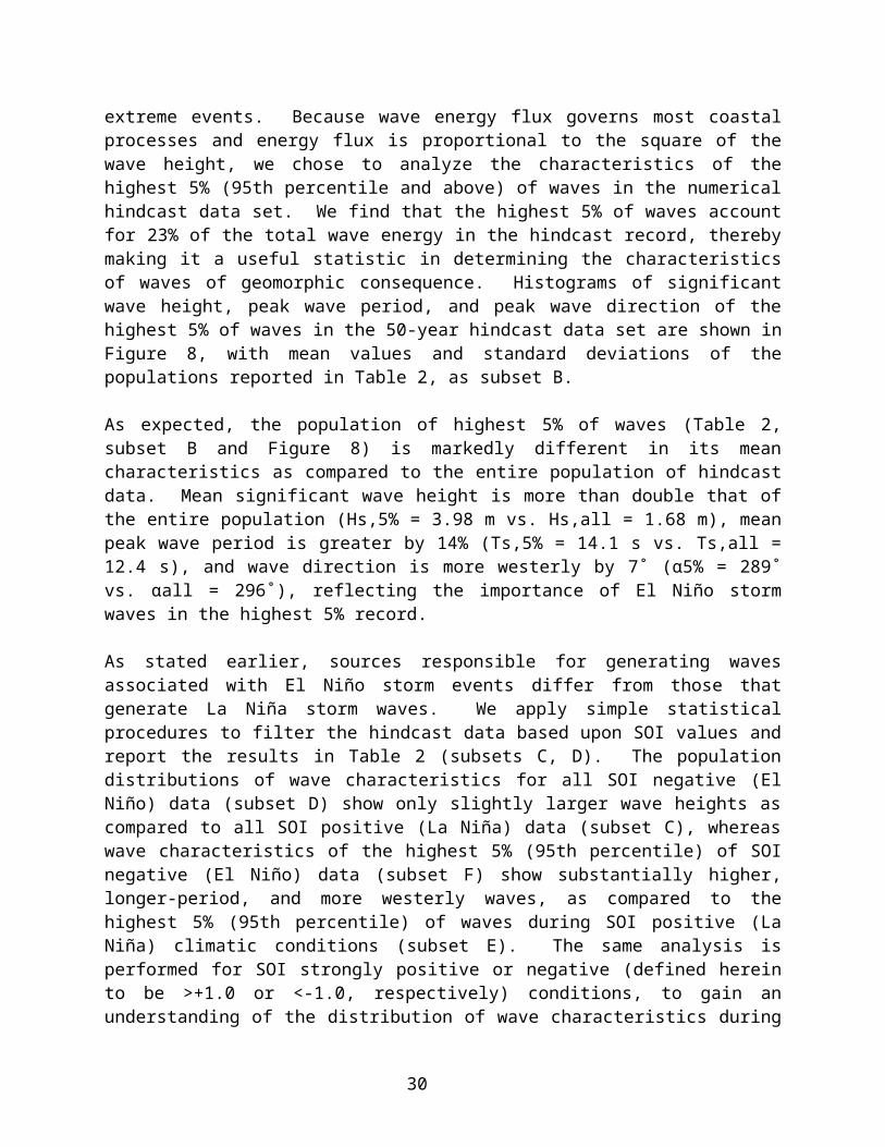
not yet backward coupled, meaning that nearshore bathymetry is not updated after a calculation of divergence of drift is conducted. Hence, the model should not be run over a time series of changing wave conditions to simulate the evolutionary behavior of a coast. In this paper, we present the results of instantaneous scenarios of divergence of drift for individual sets of deep-water wave conditions.

3.6 Model Inputs

The coastal evolution model, which consists of the wave transformation portion (SWAN) and the longshore sediment transport portion (CGEM), requires only two general inputs: bathymetry and offshore (deep-water) wave conditions. In subsections 2.2.1 and 2.2.2, we describe the details, requirements, and formats of these two general inputs.

3.6.1 Bathymetric Data

Ocean bathymetry (i.e., underwater topography) exhibits a strong control on the direction and rate of wave energy translation. Linear Airy wave theory, used when wave height is much smaller than wavelength and water depth, predicts that wave orbital motions interact to a depth of approximately half the wavelength (Komar 1998). When the water depth is shallower than half the wavelength, interaction of wave orbitals with the sea floor causes shoaling transformation and refraction of waves. Therefore, the spatial pattern of nearshore wave energy depends strongly on the distribution of seafloor elevation. A review of some studies that investigated how bathymetric changes influence shoreline change by altering shoaling and refraction patterns is provided by (Bender and Dean, 2003).

Bathymetric data are required for SWAN model simulations of wave transformation. Although, SWAN can accept bathymetric data in many formats, we chose to use a grid of bathymetry of the Southern California Bight sea floor with a spatial resolution of 3 arc-seconds (~93 meters latitudinal spacing, ~77 meters longitudinal spacing), ranging from 32˚ to 35˚ north latitude and -121˚ to -117˚ longitude (3600 by 4800 = 1.728e6 grid cells).

Bathymetric data used in this study were obtained from the National Geophysical Data Center (NGDC–NOAA) 3 arc-second U.S. coastal relief model grid database. This database provides coverage of nearshore, shelf, and proximal deep ocean bathymetry for the coterminous U.S. coastline, including Hawaii and Puerto Rico.

By using a grid-based bathymetry, changing sea level is a trivial matter performed simply by adding a scalar value to each element of water depths in the bathymetric matrix. This is further simplified by the seamless coverage of the database from offshore to onshore terrain.

3.6.2 Offshore Wave Climate

To proscribe wave climate for the SWAN module, information on wave height, period, and direction for the wave field must be provided. For wave height, some representation of the

30

central tendency must be provided; in all of our simulations, we provide significant wave height, which is defined as the average of the height of the largest one-third of the waves as measured over a specific time interval. For wave period, we provide a spectrally dominant, “peak” period and assume a Joint North Sea Wave Project (JONSWAP) distribution of frequency for the remainder of the spectrum (Hasselmann et al. 1973). For the wave direction, we provide a spectrally dominant wave direction and a “spread angle” whose cosine is calculated to account for the remainder of energy distribution within the directional spectrum.

To provide an instantaneous snapshot of the wave field in the region, a stationary SWAN run is conducted using the three specific wave climate variables, as described above. The output result is the complete stationary wave field (values of height and direction) at each grid point within the model domain. According to Airy wave theory, the wave period is not expected to change, but values may differ from the mean, dominant period, as the JONSWAP distribution is used as an input.

The wave data set used in this study comes from the numerical hindcast for the 50-year period 1948–1998 described in Graham and Diaz (2001) and Graham (2003). The wind forcing for the wave data comes from the NCEP-NCAR reanalysis project (Kalnay et al. 1996; Kistler et al. 2001). This data set represents the last full cycle of decadal climate change (full PDO cycle). The hindcast domain is the North Pacific Ocean (20˚N–60˚N, 150˚W–110˚W) with a spatial resolution of 1˚ latitude x 1.5˚ longitude. Data were produced for winter months (DJFM), with 3 hourly spectra recorded in 20 frequency bins (covering the wave period range of ~ 4.5 s–26 s), and 5 degree directional resolution grouped in 72 bins. The summary outputs used in this study, calculated from wave energy in the spectral bins, are (1) significant wave height (Hs) in deep water, (2) peak (spectrally dominant) wave period of the significant wave height (Ts), and (3) peak (spectrally dominant) wave direction (), for the reference deep-water location 33˚N, 121.5˚W; a hindcast node in the model domain. This location was chosen for its position west (oceanward) of the Channel Islands in the SCB. This location has the advantage of representing an open ocean wave climate signal, not subject to island sheltering, shoaling, and the complex refraction and diffraction patterns within the SCB, discussed by Pawka (1983), Pawka et al. (1984), and O’Reilly and Guza (1993).

For current wave time series data available for numerous sites along the U.S. coast, the reader is referred to the NOAA National Buoy Data Center (NDBC) website:

www.ndbc.noaa.gov/ and the Coastal Data Information Page (CDIP): http://cdip.ucsd.edu/.

3.7 Wave Transformation Modeling

SWAN, short for Simulating WAves Nearshore, is a 3rd generation, finite-difference, wave model that operates on the principle of a wave action balance (energy density divided by relative frequency) (Holthuijsen et al., 1993; Booij et al., 1999). In the absence of wind forcing, this model requires only two general inputs to perform a computation of the wave field throughout a region - bathymetry and deep-water wave conditions.

31

Although SWAN is written in FORTRAN, as part of this project we have written a series of MATLAB .m-files to write the required input files for SWAN (.swn files) and execute both the main grid and nested grid calculations of wave transformation.

By “main grid” calculations, we refer to the coarsely spaced (30 arc-second) initial pass SWAN computation (in stationary mode), which solves for the complete 4˚ x 3˚ grid field of wave conditions over the entire Southern California Bight. This results in a 480 x 360 matrix of wave heights, periods, and directions, wherein each value represents the conditions for a ~0.75 km2 area of sea-surface. Once the main grid (coarse) wave conditions have been computed, these values are used as boundary conditions at the oceanic edges of the nested grid locations. The relationship of grid sizes and spacing for main grid and nests are shown in Figure 2-2.

Smaller, high resolution grids (3 arc-sec), referred to herein as “nests”, were used to evaluate local wave conditions on a finer spatial scale. These nests each occupy areas within the domain of the main (coarse) grid (Fig. 3), resulting in each cell of output representing wave conditions over a 0.0072 km2 area of sea surface.

At the western and southern margins of the coarse grid, deep-water wave conditions are proscribed as boundary conditions, consisting of significant wave height, peak period with a JONSWAP frequency distribution (Hasselmann et al., 1973), and peak direction with a cosine square spread of 15 degrees. The wave field is computed from the grid boundaries over the input bathymetry to the coast. Example results from a SWAN run for the coarse grid are provided in Figure 3. From the SWAN output of the coarse grid, the boundary conditions for the individual nests were obtained (examples provided in Figures 4 and 5). Because the goal of the investigation was to examine "snapshots" of longshore distribution of erosion/accretion patterns resulting from various deep-water wave scenarios, all SWAN runs conducted in this study were performed in stationary mode. Temporally evolving wave fields, such as those produced during a storm were not examined, thereby avoiding the problem of swell arrival timing often associated with stationary runs (Rogers et al., 2007).

The wave transformation modeling was conducted on a 3-node (6 processor) Linux cluster at the University of Florida Geomorphology Lab, where we were able to take advantage of parallel processing computations. As an example to demonstrate the advantage of parallel processing for the wave transformation modeling, we provide the following comparison. A typical SWAN run for the entire Southern California Bight including separate runs for three nested subsections is executed in approximately 21 minutes on an Apple Mac Pro (2.8 GHz, Quad-Core Intel Xeon Processor) in single processor mode. The same simulation requires only 3 minutes to complete on our Linux cluster, resulting in a ~700% increase in computational efficiency.

3.7.1 Lookup Table Development

We reasoned that the most effective way to simulate long time series of wave transformation within the Southern California Bight was to develop a three-dimensional

32

lookup table of deep-water conditions for wave height, wave period, and wave direction. This method was introduced by Ruggiero et al. (2006) and proved to be an efficient technique for simulating long-term shoreline change. By doing so, any triplet of wave conditions could be approximated by the closest values for which a SWAN simulation had already been conducted. For example, if the deep water wave conditions were: Hs= 2.1 m, Tp=12.7s, and Dd=292˚, the closest triplet of conditions would be Hs=2.0m, Tp=13.0s, and Dd=290˚. This technique significantly speeds analyses, as each triplet of wave conditions can be ”looked-up” to its nearest proxy triplet—an operation that takes a fraction of a second of computer execution time, as opposed to re-running SWAN for the specific set of conditions, which would take approximately 2–3 minutes of computation time (or ~21 minutes when not employing parallel processing.)

We define the interval spacing for the three offshore wave climate variables in the lookup table by examining the joint distributions of the three offshore wave climate variables from the numerical hindcast for the 50-year period 1948–1998 described in Graham and Diaz (2001) and Graham (2003), described in Section 2.2.2, above. These joint distributions are shown in Figures 2-3, 2-4, and 2-5. The complete set of SWAN runs for the lookup tables, at two separate sea level conditions—(a) modern day sea level, and (b) + 1 meter above modern day sea level—are illustrated graphically in Figures 2-6 and 2-7. These figures show the unique deep-water wave input conditions (Hs, Tp, and Dd) used for each SWAN run, whose numbers are identified on the horizontal axis. Over a three-month period (May–July, 2008) 7,392 SWAN main grid runs and 36,960 nested grid runs were executed to generate these lookup tables, whose permutations span the following range of conditions:

Deep-water significant wave height (Hs) varies from 0.5 to 5.5 m, with an interval spacing of 0.5 m (11 conditions).

Deep-water peak wave period (Tp) varies from 9 to 20 seconds, with an interval spacing of 1 s (12 conditions).

Deep-water dominant wave direction (Dd) varies from 220 to 355 degrees, with an interval spacing of 5 degrees (28 conditions).

The product of each variables’ number of conditions (11*12*28) is the total number of permutations of wave triplets. The total number of SWAN main grid runs executed for the current sea level state was 3,696. For each main grid wave triplet condition, five nested grids were executed, resulting in 18,480 nested grid runs. Then all of the described offshore wave triplet inputs were re-run at a +1 meter sea level condition, resulting in a grand total of 44,352 SWAN model runs of wave transformation.

3.7.2 Wave Input Snapping

Utilizing a proxy wave climate and evenly spaced conditions of wave height, period, and direction in the aforementioned lookup tables requires that slight approximations will be made when attempting to simulate historical wave conditions. However, these approximation errors are most egregious, by percent of actual value, for low values of wave height and period. Fortunately, at these low values, longshore sediment transport is minimal. We expect few, if any, computation errors to arise from the “approximated” wave

33

input time series, when compared to the “actual” time series. Figure 2-8 shows an example of the hindcast wave time series and its synthesized approximation through use of the SWAN lookup table.

3.7.3 Far Field Grid Wave Field Computation (Coarse Resolution)

Figure 2-9 provides examples of the SWAN computation for the entire Southern California Bight wave field, under various wave height and period conditions for a northwesterly wave direction. These simulations are run at the coarse resolution of 30 arc-seconds, or approximately 1 km grid spacing. Notice the prominent sheltering effects of the Channel Islands. Also apparent in these simulations is the profound effect of wave period on refraction (wave steering in shallow water); a point that will be revisited during analysis of the numerical experiment results later in this paper.

3.7.4 Near-field Grid Wave Field Computation (Fine Resolution)

Figure 2-10 provides examples of the SWAN computation for the Santa Barbara nested grid within the northern portion of the Southern California Bight wave field. These simulations are run at a fine resolution of 3 arc-seconds, or approximately 90-meter grid spacing. As in the case of the main grid above, arrows on the diagram illustrate wave ray direction, which further underscores the effect of wave period on the steering of wave rays due to refraction in shallow water.

3.8 Longshore Sediment Transport Modeling

The final output from the SWAN component of the coastal evolution model is a complete oceanic grid of significant wave heights and directions (Hs and D, respectively) at each “wet node” within the model domain. In accordance with the physics of wave transformation, wave period does not change throughout the computational grid. The task of the CGEM component of the coastal evolution model is to convert the modeled wave field into the alongshore distribution of regions of sedimentary erosion and accretion, i.e., the locations and magnitudes of erosional “hotspots.” In subsections 2.4.1–2.4.8 below, we provide the details of these calculations and illustrate the numerical steps necessary to go from a nearshore wave field to a calculation of coastal erosion potential. For the sake of continuity, we will develop an example case calculation of coastal erosion potential for an instantaneous set of wave conditions.

We note that the specific form of the equation for longshore sediment transport used herein is just one of several possible options that have been developed by researchers in recent years. Various other formulations of longshore sediment transport are available and can easily be substituted into our CGEM modular-based model. Examples of the range of longshore sediment transport formulations include Inman and Bagnold (1963), Komar and Inman (1970), the CERC (Coastal Engineering Research Center) equation (Rosati et al. 2002), Kamphuis et al. (1986), Kamphuis (1991), and Bayram et al. (2007). We chose the Komar and Inman (1970) sediment transport formulation, later updated by White and

34

Inman (1989), as it was developed from direct measurements along the California coast, thereby appropriately accounting for the regional wave climate and sedimentary character of the region considered in this study.

3.8.1 Choosing the 5-meter Isobath

The first step is to select a consistent location at which to query the SWAN modeled wave field. Ideally, this selection should be based on the point of wave breaking, when the shoaling wave releases its energy by breaking and converts the broken wave energy to nearshore currents. However, the depth at which wave breaking occurs is dynamic, being highly dependent on the wave steepness, which has both wave height and period dependence (Kaminsky and Kraus 1993). Typical ranges for breaking depths are 8 to 2 meter water depth, as calculated by the relationship provided in Komar and Gaughan (1972). To avoid this complication, we select the 5-meter isobath as the location at which we query the SWAN results and discuss this model limitation in Section 2.5 below.

In the CGEM model, this is done by numerical routines, which apply MATLAB’s contouring algorithm to each of the bathymetric nests (SntBrb, SntMnc, SnPdro, DanaPt, and TorPns) to locate the map view coordinates of the 5-meter isobath. The uncorrected 5-meter isobath locations must then be quality-checked by the user, to remove closed contours in the nearshore, and distant “anchor points” that MATLAB establishes to reference the reported contour position locations. Some degree of correction must be conducted for each specific nest, as shown in the examples provided in Figures 2-11 and 2-12.

3.8.2 Decimating Along the 5-meter Isobath

After the corrected, 5-meter isobath is chosen for each nest, a consistent spacing along the isobath must be calculated, so as to have an even alongshore distribution of modeled nearshore wave conditions. For the numerical experiments presented herein, we selected a decimation spacing of 100 meters, yielding 586, 695, 357, 574, and 406 along-isobath model output positions for nests SntBrb, SntMnc, SnPdro, DanaPt, and TorPns, respectively. An example of the isobath decimation is provided for nest TorPns in Figure 2-13.

3.8.3 Computing Coastal Trends

An accurate measurement of the orientation of the coastline is necessary for the computation of angle of incidence ()—the difference between nearshore wave direction and coast normal direction, which is a fundamental variable in the calculation of both the radiation stress (Sxy) and the longshore component of wave energy flux (Pl), also known as the stress-flux factor. Detailed computation of coastal trends for the decimated 5-meter isobaths in each of the nested grids was performed by the following procedure:

Starting at the northwest-most portion of the isobath, window 10 adjacent, decimated model output positions as a subset (~1 km).

Fit a linear regression orientation line to the subset, using the widest range spatial orientation (latitude or longitude) as the independent variable. This ensures that

35

shorelines with a more north-south trend are fit with longitude as the independent variable and that shorelines with a more east-west trend are fit with latitudes as the independent variable.

Record the direction of the normal to the fitted trendline (90˚ clockwise from trend) as the shore-normal value for the midpoint location of the subset.

Slide the window downcoast (toward the southeast) by one model output position and repeat the steps above.

Stepwise regression and correction calculations are provided in Figure 2-14. Shore normal orientations for two nested grids are plotted on maps in Figure 2-15.

3.8.4 Retrieving and Interpolating SWAN Output

The task of obtaining model output at the decimated model output positions is performed by simply conducting a two-dimensional linear interpolation of the SWAN nested grid results for wave height and direction. After retrieval, the alongshore wave heights and directions are smoothed with a 1-km moving average window.

3.8.5 Calculating Angle of Incidence

A major control on longshore sediment rate is the longshore component of wave energy flux. The angle of incidence is of primary importance in the calculation of longshore sediment transport, as will be further discussed in subsection 2.4.7. If wave rays approach the beach at an angle perfectly orthogonal to the trend of the coast, the longshore component of wave energy flux is zero, and there is no net longshore current to drive longshore sediment transport. If wave rays approach the beach at an oblique angle (somewhere between orthogonal and parallel), there is a component of wave energy flux parallel to the shoreline, which drives longshore sediment transport.

The calculation of angle of incidence in the CGEM model is quite straightforward and proceeds as follows: Assuming a north-south trending coastline with land to the east and sea to the west, the angle of incidence is the difference between the nearshore wave direction (azimuth) and the coast normal (azimuth). Two scenarios are described below. In scenario A, nearshore waves approach from the northwest (D~300˚) and the coast normal is approximately due east, referenced by the direction from which the vector originates (N~270˚), making the angle of incidence () equal to approximately +30˚. Longshore currents generated for scenario A would be directed southward. In scenario B, nearshore waves approach from the slightly south of west (D~265˚) and the coast normal is approximately due east, as in scenario A (N~270˚), making the angle of incidence () equal to approximately -5˚. Longshore currents generated for scenario B would be directed northward, with decidedly less magnitude.

3.8.6 Calculating Wave Energy Flux

Wave energy flux P, which has dimensions of [mass•length/time3] and units of [Watts/meter of shoreline], is calculated through the relationship

36

P=ECn=18ρw gH

2Cn

where E is wave energy density, which has dimensions of [mass/time2] and units of [joules/meter2], C is nearshore wave celerity, which is depth controlled and has dimensions of [length/time] and units of [meters/second], n is ratio of group to individual wave speed (~1 in shallow water) and is dimensionless, is the density of seawater [1024 kg/m3], g is gravitational acceleration [9.81 m/s2], and H is nearshore wave height, which has dimensions of [length] and units of [meters], as computed by the SWAN portion of the model and interpolated along the decimated 5-meter isobath.

The longshore component of wave energy flux, Pl, is calculated by simply multiplying the wave energy flux, P, by the trigonometric functions that provide the component parallel to shore

Pl=Psin α cosα

where the sine and cosine terms result from the tensor transformation of the onshore flux of longshore directed momentum that is embedded in Pl (Longuet-Higgins and Stewart 1964). Procedure for calculation of angle of incidence, , is described in Section 2.4.5., above. Example stepwise calculations of wave energy flux for the SntMnc grid are shown in Figure 2-16.

3.8.7 Calculating Divergence of Drift

The formulation of longshore sediment transport calculation used in the CGEM model comes from the sediment-transport theories of Bagnold (1963), Inman and Bagnold (1963), and Komar and Inman (1970). These theories utilize the concept of immersed-weight sediment transport rate (Il) to account for density of sediment grains,

I l=KPl

where Kl represents a dimensionless coefficient of proportionality, as defined by Komar and Inman (1970), and is set to a value of 0.8 for all of the numerical experiments described below. Immersed-weight transport rate is converted to volumetric transport rate through the relationship

37

Ql=I l

( ρs−ρw )gNo

where s and w are densities of quartz sediment (2650 kg/m3) and seawater (1024 kg/m3), respectively, g is the gravitational acceleration constant (9.81 m/s2), and No is the volume concentration of solid grains, set to 0.6, for all numerical experiments described below.

The calculation of the volumetric rate of longshore sediment transport yields a rather noisy result. To obtain a more reasonable estimate of local trends in longshore sediment transport, we smooth the calculations of longshore transport with a 1-km moving average window (Figure 2 17).

The last remaining step to obtain volumetric estimates of gradients in longshore transport (also known as the divergence of drift) is to perform a discretized differential of volumetric rate of longshore sediment transport with respect to alongshore position.

Ñ⋅Ql=¶Ql¶ x

This quantity is, effectively, the calculated change in sediment volume over the longshore reach dx, during the time interval that these wave conditions are applied. Herein, we adopt the sign convention that divergence is defined as the net difference between sediment inflow and sediment outflow, making positive divergence of drift (where inflow exceeds outflow) result in accretion at a site, whereas negative divergence of drift (where outflow exceeds inflow) results in erosion. The longshore pattern of divergence of drift is therefore out of phase with longshore sediment transport, as expected. At longshore positions where transport is increasing at the greatest rate (positively sloping inflection points), divergence of drift is at a local minimum; where transport is decreasing at the greatest rate (negatively sloping inflection points), divergence of drift is at a local maximum; where transport is at a local minimum or maximum, divergence of drift should be zero.

3.9 Model Limitations

The use of a three-dimensional lookup table to approximate time series of wave conditions presents the drawback that precise conditions are not used as inputs for deep-water wave conditions in the SWAN wave transformation calculations. Although this is an approximation, we have set the interval spacing for wave heights, periods, and directions in the lookup table sufficiently small that we expect inaccuracies arising from the imprecision of inputs to be minimal.

We acknowledge the assumption that the 5-meter isobath is representative of nearshore wave conditions should be taken into account appropriately. Under conditions of milder wave fields, wave breaking will be landward of the 5-meter isobath, and for similar

38

considerations, wave breaking under conditions of highly energetic wave fields will be seaward of the 5-meter isobath location. However, for most wave fields the break point will be landward of the 5 meter isobath, and in these cases, we can rely on the conservation of wave energy flux to protect our assumption.

It should be noted that the calculations of divergence of drift, described in Section 2.4.7, are potential divergence of drift, assuming that we have a transport-limited longshore drift scenario, meaning that we are calculating the total amount of longshore transport of sediment if an unlimited supply was available. This is not likely the case for much of the Southern California coast, as river-damming and the arid environment tends to make the littoral system supply-limited in many places. Where the wave energy demands on sediment transport exceed the supply, bedrock platforms will be exposed and erosion of sea cliffs will proceed with greater efficiency.

3.10 Numerical Experiments

Given the wide range of possible numerical investigations suitable for a modeling study of the influence of climate change on coastal evolution, we designed and conducted two separate scientific investigations that employ the modeling procedure described above, for several study sites within the Southern California Bight (Sections 3.1 and 3.2).

The first investigation examined the effect of wave direction on magnitude and location of longshore sediment transport and drift divergence along the eastern portion of the Santa Barbara County coast and along the San Diego County coast. The second investigation is a probabilistic evaluation of likelihood for erosional hotspot development along the coast of Los Angeles and Orange Counties given the known frequency of El Niño winters and Pacific Decadal Oscillation over the past half-century.

The specific study sites, selected for the various numerical experiments, represent distinct orientations with respect to the Pacific Ocean: (1) east-west trending, south-facing coast (the eastern reach of Santa Barbara County coast – ”SntBrb”), (2) cuspate shaped with smoothly varying orientation from south-to-west facing coast (the Santa Monica Bay and Orange County coasts – ”SntMnc,” “SnPdro,” and ”DanaPt”), and (3) north-south trending, west-facing coast (the central San Diego County coast – ”TorPns”). Locations and close-up views of these sites are provided in Figures 1-1 and 1-2.

3.10.1 Wave Direction Experiment

To provide insight on how climate change-driven alteration of deep water wave conditions might affect the magnitude of erosion and accretion along the Southern California coast, we conducted a series of controlled numerical experiments at two physiographically-distinct, reaches of the Southern California coast, which we refer to as the Santa Barbara (SntBrb nest) and Torrey Pines (TorPns nest) sites. The goal of these experiments is to test the hypothesis that deep water wave direction exhibits critical control on the longshore sediment transport patterns at coastal sites within the bathymetrically complex SCB. Each

39

of the locations chosen witness unique swell patterns resulting largely from their relative orientations with respect to the deep water wave field of the North Pacific Ocean, each site's local shelf bathymetry, and the blocking patterns that the Channel Islands provide to each site (Fig. 3). The two sites represent end member coastal orientations within the Bight; the SntBrb nest exhibits a west-to-east general shoreline orientation, whereas the TorPns nest exhibits a north-to-south general shoreline orientation. For each experiment, we conducted 104 SWAN-CGEM simulations that vary deep water wave direction from 260˚ to 320˚ in 5˚ intervals for four pairs of wave height period scenarios: (1) H=2 m, T=12 s, (2) H=2 m, T=16 s, (3) H=4 m, T=12 s, (4) H=4 m, T=16 s. These ranges span the distributions of deep water wave conditions documented for the SCB by Adams et al. (2008).

3.10.1.1 Site 1 - Santa Barbara

The western end of Goleta Beach, adjacent the UCSB campus in southeastern Santa Barbara county, California, has been the site of regular nourishment due to chronic sand loss and the community desire to maintain a recreational beach. The site has witnessed profound changes in beach width, morphology, and sediment volume over the past 30 years with anecdotal photo histories documenting wide, well-vegetated, sandy beaches in the 1970's, which were fully inundated during the El Niño winters of 1982-83 and 1997-98 (Sylvester, 2010). Waves entering the Santa Barbara channel, as swell, have been modeled by (Guza et al., 2001), and are regularly forecasted by the Coastal Data Information Program, CDIP.

3.10.1.1.1 SWAN Transformed Wave Field

SWAN output from a moderate, westerly swell (H=2 m, T=12 s, = 270˚) is shown in Figure 4. The wave height distribution pattern for the entire SCB (Fig. 4A) illustrates the blocking effect of the Channel Islands. Fig. 4B shows the decrease (by more than half) in wave height as waves enter shallow water. Fig. 4C shows the significant amount of refraction that occurs as waves approach the nearshore and the significant sheltering experienced by the Goleta Beach site, herein referred to as SB-2 (blue star), as compared to the exposed site SB-1 (red star) located immediately west of Goleta Point, 1 km from SB-2.

3.10.1.1.2 CGEM Results

It is instructional to observe the results of two CGEM simulations plotted along shore in the vicinity of SB-1 and SB-2. Figure 6 shows the strong influence exerted by wave direction at the Santa Barbara site. Output from two SWAN simulations are passed to CGEM to examine longshore patterns of potential sediment transport rate and divergence of drift. For each SWAN simulation, deep water wave height and period are set to 4.0 m and 16 s, but the deep water wave direction is 320˚ (northwesterly) in case A, representative typical La Niña storm wave conditions, as opposed to 270˚ (westerly) in case B, representative of El Niño storm wave conditions, during which time the jet stream occupies a more southern position than usual due to the anomalous atmospheric pressure distribution (Storlazzi and Griggs, 2000). Comparison of the two deep water input cases is as follows. Along the 5-meter isobath, the significant wave height for Case A (northwesterly) is very small (<0.5

40

m), in comparison to deep water inputs conditions (Hsig=4 m), everywhere along the 5 km reach. For Case B, the wave heights are substantially higher, approximately 2 meters everywhere along the reach. The angle of incidence varies for both Case A and Case B, but in the same pattern, developing a sizable longshore component of wave energy flux. The longshore sediment transport rates vary in much the same manner as wave heights for the two cases, with appreciable transport in Case B, and negligible transport in Case A. The potential divergence of drift pattern for Case B shows loss of sediment (erosion) at SB-1 (red star) and gain of sediment (accretion) at SB-2 (blue star). Potential divergence of drift is negligible along the length of the 5 km reach for Case A.

3.10.1.1.3 SntBrb Experiment

The 104 SWAN-CGEM simulations which were run for the SntBrb experiment produced divergence of drift patterns which are reported for SB-1 and SB-2 in Figure 7. This compendium of experiment results illustrates that the exposed SB-1 site experiences increasing erosion as wave conditions become more westerly. This is in contrast to the sheltered SB-2 site, which becomes more accretionary as wave direction becomes more westerly. Increasing deep-water wave height causes enhancement of erosional or accretional behavior at both SB-1 and SB-2, depending on the site tendency under milder conditions. Increasing wave period causes enhanced erosion at SB-1, but causes decreased accretion at SB-2.

3.10.1.2 Site 2 - Torrey Pines

Torrey Pines beach, located approximately 7 km north of Scripps Pier in La Jolla, California, has been the site of many scientific inquiries in the field of coastal processes (Thornton and Guza, 1983; Seymour et al., 2005; Yates et al., 2009). The relatively straight, north-south trending reach resides within the Oceanside littoral cell and owes any longshore variation in wave energy flux to the blocking effects of the Channel Islands, rather than to complexities of nearshore bathymetry, save for the areas around the Scripps and La Jolla submarine canyons in the southern portion of the TorPns nest.

3.10.1.2.1 SWAN Transformed Wave Field

As for the Santa Barbara site discussed above, we show the behavior of the Torrey Pines site to a SWAN simulation for a moderate, westerly swell (H=2 m, T=12 s, = 270˚) in Figure 5. The demonstrable change in wave height visible around 33.05˚ north latitude in Figure 5B is a result of waves penetrating through a window between Santa Catalina and San Clemente Islands during periods of westerly swell. The general shore-normal orientation of the wave field (for input conditions shown) promotes nearshore wave height increase as a result of shoaling in the absence of refraction.

41

3.10.1.2.2 CGEM Results

Comparative examples of CGEM simulations from the TorPns nest for Cases A and B (described above in Section 4.1.2) are given in Figure 8. Just as for the SntBrb nest, the significant wave height for Case A along the 5-meter isobath in the vicinity of Torrey Pines sites TP-1 and TP-2 is very small (<1.0 m). However, in the TorPns nest, this may be due to blockage of waves by the Channel Islands rather than to severe refraction as in the SntBrb nest. Angles of incidence for both case A and B at TorPns are small, approximately less than +/- 5˚. For case B, between kilometer markers 23 and 25.7, angle of incidence is negative which results in northward-directed longshore sediment transport pattern in this region, as opposed to the southward directed transport elsewhere in the nest. For case A, divergence of drift pattern is negligible everywhere within the 5 km span surrounding TP-1 and TP-2, whereas for case B, a strongly negative potential divergence of drift (erosion) emerges at Torrey Pines Beach, near TP-1 and TP2.

3.10.1.2.3 TorPns Experiment

As for the SntBrb nest discussed in Section 4.1.3, the 104 SWAN-CGEM simulations, which were run for the TorPns experiment produced divergence of drift patterns which are reported for TP-1 and TP-2 in Figure 9. All simulations run for the Torrey Pines site resulted in erosion. At TP-1, the peak in magnitude of potential divergence of drift occurs when waves are just north of westerly (275˚ - 290˚). Increases in wave period slightly increased erosion for 2 meter waves, and shifted the peak direction for maximum erosion for 4 meter waves, at TP-1. At TP-2, wave height has a profound influence; doubling of the deep water wave height causes potential divergence of drift to approximately triple across the directional range. Increasing wave period, however, had negligible effect at site TP2.

3.10.2 Erosional Hotspot Likelihood Experiment

The second set of experiments targets a probabilistic evaluation of likelihood for erosional hotspot development along the coast of Santa Monica Bay, given the known frequency of El Niño winters and Pacific Decadal Oscillation over the past half-century. Using the aforementioned numerical hindcast of Graham and Diaz (2001) for deep-water winter wave heights, periods, and directions for the period 1948–1998, we use the SWAN-CGEM model to calculate estimates of annual potential beach volume change for 14 specific beaches within the Santa Monica Bay region. Results from this experiment will give a modeled history of locations of erosional hotspots for the years 1948–1997. We selected these beaches on the basis of their utility for the coastal economics study by Pendleton et al. (2008), sponsored by the California Energy Commission’s Public Interest Energy Research (PIER) Program. The names and locations of the beaches are provided on the maps in Figure 3-5 and in Table 3-2.

42

3.10.2.1 Experimental Design

The development of the lookup table, discussed in Section 2.3.1, enables us to write numerical codes, which loop through a time series of deep-water wave conditions; identify the closest modeled triplet of wave heights, periods, and directions; and extract the SWAN wave transformations for a selected bathymetry within the Southern California Bight. The heights, periods, and directions used in this experiment are three-hourly hindcasts for winter waves (December through March) of 1948–1998, at the deep-water site (33˚N, 122˚W) as provided by Graham and Diaz (2001) and analyzed by Adams et al. (2008). This time series of wave conditions was run through the SWAN-CGEM routines for the bathymetric nest “SntMnc,” and longshore distributions of annual potential beach volume change were calculated for the 14 beaches identified in Table 3-2. These results were used in an economic model of beach use presented by Pendleton et al. (2008), for a complementary PIER study.

3.10.2.2 Results

Model results of the 50-year analyses of patterns of potential winter erosion/accretion along the Santa Monica Bay beaches are provided in Figures 3-6, 3-7, 3-8, 3-9, and 3-10. Annual rates of potential volumetric accretion were as high as ~800 cubic meters per meter (m3/m) (Hermosa), and annual rates of potential volumetric erosion were as high as -2,500 m3/m (Torrance). Most beaches exhibited regions of consistent accretion and regions of consistent erosion. In all cases, annual potential volumetric beach change was most severe during the El Niño winter of 1982–1983, shown as a green line in Figures 3-6 through 3-10.

Figure 3-11 illustrates the daily divergence of drift calculated for one beach over the course of two winters: a strong La Niña winter (1973–1974) and a strong El Niño winter (1982–1983). The temporal pattern of divergence of drift during the strong El Niño winter reveals much more frequent large-scale erosional events in the erosional portion of the beach (between 54.5–56 km from Point Dume). It is notable, but perhaps purely coincidental, that the difference in timing of erosional events, when comparing the La Niña and El Niño winters, illustrates that the bulk of severe, damaging storms occur later in the winter season during El Niño winters.

3.10.2.3 Experimental Conclusions and Implications

From the erosional hotspot likelihood experiments, the following conclusions can be drawn:

For the beaches of the ”SntMnc” coastal nest, the following beaches are considered to be chronically erosional: PointDume, WillRogers, Dockweiler, and Torrance. Only two beaches, DanBlocker and LasTunas, are considered to be continuously accretional. And the remaining eight beaches (Malibu, Topanga, SantaMonica, Venice, ElSegundo, Manhattan, Hermosa, and Redondo) are mixed in their trend of sedimentary health, exhibiting both erosional and accretional reaches. A valuable check on the modeling performed during this

43

experiment would be a comparison of these results with beach nourishment statistics for beaches of Los Angeles County.

In every beach examined, the 1982–1983 El Niño winter yielded the most dramatic potential beach volume changes, irrespective of whether those changes were erosional or accretional. This conclusion points to an important implication that highlights a consistent, recurring theme in geomorphology and Earth science; namely, that the “extreme,” relatively infrequent, events dominate landscape change. This is not a new conclusion, as numerous studies have referenced the dramatic coastal changes witnessed during El Niño winters, but the experiments conducted during this project bolster the general consensus of the geomorphological community.

Lastly, it should be noted that numerous studies have shown that beaches “recover” after an erosional event (lasting one to several days) over a time period of days to weeks. Often, the accretionary pattern associated with a recovery appears as a mirror-image of the spatial pattern of erosion the beach experiences during the storm event (e.g., List et al. 2006). Though the causes and mechanics of the recovery are not well understood, this behavior implies that a dynamic equilibrium of beach morphology exists in tune with a characteristic wave climate for a coastal region.

3.11 Summary and Implications of Longshore Sediment Transport Modeling

A numerical modeling procedure for assessing the patterns of littoral sediment transport in Southern California has been presented. The procedure combines a spectral wave transformation model with a calculation of gradients (divergence) in longshore sediment transport rates, assuming transport-limited conditions. To illustrate some specific coastal impacts resulting from climate change, we have applied this procedure to two physically-distinct sites within the SCB. We conducted a sensitivity analysis at the two study sites, whereby effects of variability in deep water wave direction were explored for four wave height / wave period combinations.

This study demonstrates that the longshore sediment transport patterns in the littoral zone, and therefore the locations of erosional hotspots, along the Southern California coast are extremely sensitive to deep water wave direction. We speculate that this sensitivity is due to two principle reasons: (1) the severe refraction required by northwesterly waves in order to be incident upon south facing coasts (e.g. SntBrb nest), which could also be considered a sheltering effect of Pt. Arguello, and (2) the sheltering effects of the Channel Islands (blocking of incoming swells and additional refraction of grazing waves) on west facing coasts (TorPns nest). Observations of wave interruption by islands were made decades ago by Arthur (1951).

Although the cross-shore transport of sediment in the littoral zone is not specifically addressed in these numerical experiments, we acknowledge its potential importance during large wave events. Long-period swells, often associated with large wave events, will increase refraction, which increases the cross-shore component of wave energy flux. Associated high wave set-up can promotes off-shore transport and the temporary storage

44

of littoral sediment in offshore bars. Despite the fact that cross-shore transport can be strong during events, the associated “erosion” is often temporary, as recovery proceeds relatively rapidly after a large wave event via onshore transport of bar sediment.

It is noteworthy that the Santa Barbara wave direction experiment illustrated how the divergence of drift at a site exposed to the open ocean (SB-1) experiences enhancement of erosion as the wave field intensifies (increased wave heights and periods), whereas the divergence of drift at a site locally sheltered by a headland (SB-2) experiences enhancement of accretion as the deep water wave heights are increased. The fact that the sheltered site experienced slight decreases in accretion for increased wave periods may be due to the higher degree of refraction that the longer period swells undergo before reaching the coast.

The Torrey Pines experiment reveals interesting behavior regarding the direction of longshore transport and erosion. As shown in Figure 8, for a westerly wave field of strong intensity (Hs = 4 m, T = 16 s, a = 270˚), the angle of incidence between position markers 23-25.75 km is negative, but changes to positive between position markers 25.75-28 km. The result of this change in angle of incidence is a change in direction of longshore transport from northward to southward. However, divergence of drift is negative for this set of deep water wave conditions at both TP-1, where transport direction is northward, and TP-2, where transport direction is southward. This persistence of erosional character at this site, irrespective of transport direction, suggests that continental shelf bathymetry may exert a unique control on nearshore wave fields at this site.

It is observed that at both SB-1 (SntBrb nest) and TP-2 (TorPns nest), negative divergence of drift (erosion) appears to operate under all deep water conditions simulated. This brings up two questions: (1) Why does the coast at SB-1 protrude seaward relative to the coast at SB-2, if the SB-1 shoreline is retreating under all simulated conditions? (2) Why does the Torrey Pines coastline maintain a relatively straight appearance if the shoreline at TP-2 is consistently retreating more rapidly than the shoreline at TP-1? Several explanations are offered to address these discrepancies and we suspect the answer is a combination of these. First, as mentioned above, the erosion/accretion portion of the CGEM model assumes transport-limited conditions, meaning that deficiencies in sediment supply are not considered to play a role in coastal landform evolution. If sediment supply is limited at these sites, then the model may overestimate the magnitude of divergence of drift. Second, the model only considers the movement of sediment alongshore at these coastal sites and does not address the rocky cliffs that back the beaches along much of the Southern California coast. During high wave conditions when sediment supply is limited, it is quite likely that beach sand is temporarily stored offshore in bars and waves directly impact the bedrock cliffs, whose retreat is not governed by Equation (4) above. To simulate shoreline retreat of an exposed cliffed coast, bare bedrock cutting processes must be adequately modeled. Neither of these caveats, however, changes the fact that the gradients in potential longshore sediment transport patterns are highly sensitive to deep water wave conditions, and particularly, to wave direction.

45

These results have implications regarding climate change, longshore sediment transport patterns, and the distribution of hotspots of coastal erosion within the SCB. Our numerical simulations illustrate a dramatic increase in absolute value of divergence of drift as wave climate approaches westerly deep water wave directions. It has been documented that during El Niño winters, waves entering the Southern California Bight tend to be more westerly than during non El Niño winters (Adams et al., 2008). Therefore, model results presented herein are consistent with the observations of severe coastal change in California during the El Niño winters of 1982-83, and 1997-98 (Storlazzi et al., 2000). Recent research investigating tropical cyclonic behavior during the early Pliocene (5-3 ma) reveals a feedback that may serve to increase hurricane frequency and intensity in the central Pacific during warmer intervals (Fedorov et al., 2010). This is relevant to Earth’s current climate trend because the early Pliocene is considered a possible analogue to modern greenhouse conditions. Federov et al. (2010) provide results of numerical simulations of tropical cyclone tracks in early Pliocene climate, which illustrate a dramatic poleward shift in sustained hurricane strength within the eastern Pacific Ocean. This pattern results in increased westerly storminess, implying that warmer climates will cause the SCB to witness greater absolute values of divergence of drift. In other words, a more volatile coastline, exhibiting higher magnitude erosion and accretion, might be expected as a result of increased frequency of strong westerly waves.

46

4. Sea Cliff Retreat Resulting From Sea Level Rise and Wave Climate Change

This section of the report presents our investigation into the question of how sea cliff retreat can be expected to occur as a result of the combined effects of an elevated eustatic sea level and an intensification of wave conditions, driven by global climate change. Herein, we present: (1) a discussion of the estimates of cliff retreat due to sea level rise alone, (2) a numerical model of sea cliff retreat resulting from the combined processes of sediment abrasion and cantilevered block failure, and (3) results from a field investigation of sea cliff mechanical process-response to the southern California wave climate. A peer-reviewed journal publication was produced from field studies conducted to help with the derivation of this model, included herein as Section 4.3. A detailed summary and interpretation of the field investigation were published in the following journal article:

Young, A. P., Adams, P. N., O'Reilly, W. C., Flick, R. E., & Guza, R. T. (2011). Coastal cliff ground motions from local ocean swell and infragravity waves in southern California. Journal of Geophysical Research, 116(C9). doi:10.1029/2011JC007175.

4.1 Estimate of Cliff Retreat Due to Sea Level Rise

Sea level rise is one of the major concerns associated with climate change. In addition to the effects of flooding/coastal inundation, there is a concern that changing water levels effectively changes the nearshore bathymetry, which may have a significant effect on the distribution of coastal wave energy alongshore. Naturally, the coastal landscape will adjust to this new distribution of wave energy by seeking a new dynamic equilibrium; accomplished by eroding some portions of shoreline and accreting others. In this section, we explore the effect of a +1 meter rise in sea level on the natural position of sea cliff, along a well-studied, stable portion of the central coast of San Diego county between 32.8˚ and 33.15˚ N latitude, identified above as the ”TorPns” coastal nest. This +1 meter rise in sea level is within the range predicted by some recent sea level rise studies for the next century, but is not based on an exact greenhouse gas emission scenario.

4.1.1 Background for Sea Level Rise Calculations

Sea level rise along coasts with sea cliffs and rock platforms always involves cliff erosion and a landward extension of the rock platform. In cases where sea cliff erosion rate cannot keep pace with sea level rise, as is often the case for cliff faces of plutonic rock, lava flows and engineered cement walls, sea level may rise against a nearly vertical sea cliff, eventually resulting in a plunging cliff coast. However, coasts with sea cliffs and platforms of more easily eroded sedimentary material usually begin to erode and adjust to the rising sea level, as shown by the many studies of submerged and emerged terraces along the California coast. Depending on the dominant process responsible for sea cliff erosion, platform and sea cliff cutting proceed most effectively when a full, protective beach cover is

47

not present. The absence of equilibrium beaches precludes the application of concepts such as the divergence of the drift and hot spot analysis. Modeling this situation requires the occasional activation of sea cliff and platform cutting modules, which is the next step in our modeling effort. However we do have a well-established understanding of the processes involved in terracing by wave action during sea level rise. This understanding leads to geometric relations that can be applied to cliff erosion and platform cutting that can be predicted from sea level rise as discussed in the following.

We select a section of coastline that is stable and has a known history of stability for millennia, such as the Torrey Pines block between La Jolla and Solana Beach in the Oceanside littoral cell. The Torrey Pines subcell from the head of Scripps Submarine Canyon to Solana Beach contains some of the most stable coastline in southern California, with a small uniform uplift rate of 0.13 mm/yr established over the past 1,525 ka by the elevation/age relationship of emergent marine terraces (Legg and Kennedy, 1979; Kennedy and Tan, 2008). However, the stability ends abruptly along the Rose Canyon fault that passes through La Jolla to the south and extends offshore to the west (e.g., Hogarth et al., 2007).

4.1.2 Estimates of the Effects of Sea Level Rise

We select the Torrey Pines subcell to illustrate the procedure for calculating the potential effect of sea level rise on the sea cliff and platform, noting that the small land uplift rate of 0.13 mm/yr is negligible in comparison to the existing sea level rise of about 3 mm/yr and the present estimated rise of about 1.4 m by the end of the century. Also, the sea cliffs and platforms consist of Eocene sedimentary formations of differing resistances to erosion (Inman et al. 2005a).

Seismic studies of the bottom and subbottom profiles show that the continental shelf off the Torrey Pines block consists of terraces cut into mostly Tertiary sediments representing stillstands of the various past sea levels. These submerged terraces supplement the emerged terraces now observed on land. In many cases the sea cliffs of the emerged terraces are steeper, representing the cliff face slope when cut before recession. However those for the submerged terraces are less steep, representing passage of the rising sea level. In both cases, the platform slopes are gentle and reflect the original wave-cut platform. Although the rate of sea level rise may enter as a factor in the slope relation for platform slopes, the major factor appears to be the erodibility of the rock formation (e.g., Inman et al. 2005b; Sunamura 1992).

In the following discussion we define the platform as the sub-horizontal bedrock surface attached to, and extending seaward (X) from the existing sea cliff base. The platform slopes at angle from the plane defined by present mean sea level (MSL). The relation is shownβ schematically in Figure 4-1 for present sea level, with a landward position to accommodate future sea level rise (SLR’) and sea cliff erosion (SCE’). The slope of the present platform is given by the relation

tan = h/X

48

while that for the future platform (') may be slightly greater or less.

For purposes of comparison, we assume that the composition of the future sea cliff and platform remain the same as the present so that to a first approximation, 'is equal to . Future wave forcing may increase as a result of climate change, while future rates of sea level rise will certainly increase. Since the slope of the platform is likely to decrease with increasing wave intensity and increase with increasing rate of sea level rise, the two effects may partially cancel one another.

Analysis of the platform slopes for the six seismic profiles of platforms measured along the Torrey Pines subcell show that the slopes adjacent to the sea cliffs range from about 1.0%β to 2.9%, with a median value of about 2.1%. A slope of 2.1% suggests that a sea level rise of 1 meter could result in a sea cliff retreat of about 47 m, while an estimated sea level rise of 1.4 m by 2100 AD will cause a cliff retreat of 67 m. The present sea cliff retreat rate of about 5 cm/yr (Young and Ashford 2006) would result in a retreat of 4.5 m by 2100 AD. This suggests we can expect coastal cliff erosion to increase by factors of 10 to 15 times the present rate.

The calculation presented above is based largely on simple extrapolation, which sheds no light on the mechanical processes at work in the sea cliff geomorphic system. The following section presents a process-driven numerical model that can be linked with the longshore sediment transport model presented in Section 3 of this report, in order to provide estimates of cliff retreat rates for a range of sediment supply and wave climate scenarios that may accompany climate change.

4.2 Numerical Modeling of Cliff Retreat Due to Changing Wave Climate

The numerical modeling presented in this portion of the report reveals the temporal heterogeneity, which inherently exists in the process of sea cliff retreat. This erosion style, that of “fits and starts” owes its origin to the feedbacks associated with abrasion by sediment, cantilevered cliff failure, and comminution of failed cliff material.

4.2.1 Introduction

Rocky and cliffed coast retreat is episodic with failures often linked to individual storm or seismic events (Komar and Shih, 1993; Benumof et al., 2000; Hapke and Richmond, 2002). Correspondingly, climate and tectonic activity have been suggested as the major drivers of long-term rocky coast evolution (Emery and Kuhn, 1982). Multiple marine and subaerial factors have also been recognized as important to cliff erosion, such as waves (Wilcock et al., 1998; Ruggiero et al., 2001; Adams et al., 2002; 2005), groundwater flow (Lawrence, 1994; Pierre and Lahousse, 2006), beach geometry (Sallenger et al., 2002; Trenhaile, 2004), cliff lithology (Sunamura, 1992; Collins and Sitar, 2008), mechanical and chemical weathering (Sunamura, 1992; Porter and Trenhaile, 2007), and rainfall (Young et al., 2009). Sea level oscillations are also important to rocky coast evolution over longer time

49

scales (>100 k.y.), yet their precise control on erosion rates are not straight-forward and, at times, contradictory (Ashton et al., 2011).

These characteristics coalesce to form a simplified concept of consolidated sea cliff retreat: during elevated sea levels (i.e. storms, high tides) waves impact the base of the cliffs, which may be weakened through weathering, fatigue, or rainfall, and exert both hydraulic forces (e.g. wave quarrying, water hammer, air compression) as well as mechanical abrasion if sediment particles are available. These forces lead to progressive undercutting (notch development) until the upper cliff fails. Seismic activity and/or sea level fluctuations are notably important for varying the horizontal plane on which the waves act. In the case of shore platform submergence, wave energy may not be attenuated as efficiently, causing greater erosion at the cliff face. Conversely, uplift can prevent (likely temporarily) waves from accessing the cliff face. These concepts – minus detailed attention to mechanical abrasion – have been adopted by modelers to explore long-term shore platform development (e.g. Trenhaile, 2000) as well as mesoscale cliff erosion (e.g. Walkden and Hall, 2005); because of the longer temporal scales of these works, failure criteria were not incorporated.

Sunamura (1982a, 1992) showed in laboratory tests that cliffs and adjacent beaches can have internal feedbacks. The amount and configuration of beach material can enhance wave efficacy by providing abrasive agents (positive feedback) or by preventing waves from breaking near the cliff toe when a robust beach above mean sea level is present (negative feedback). The system is further complicated by the introduction of debris material after a failure, which waves must first comminute before resuming cliff undercutting. Additionally, a portion of the talus may provide suitable beach material that augments the platform beach. Limber et al. (2011) have applied these concepts to a numerical model that explore the long-term evolution and equilibrium of rocky coasts. In this study, we use a numerical model to explore the plausibility of internal sediment, failure, and comminution feedbacks as a driver of temporally (and spatially) episodic cliff evolution – even in the absence of major storm or seismic events.

4.2.2 Background

Rocky coasts are cliffed shores composed of consolidated materials ranging from hard rock (e.g. granite, basalt) to soft glacial deposits (Trenhaile, 1987; Sunamura, 1992). Unlike beaches that experience accretion and erosion vacillations, rocky coast evolution is a one-way progression of retreat (Sunamura, 1992; Davidson-Arnott, 2010). Assailing efficacy originates from subaerial weathering and mechanical wave erosion (Trenhaile, 1987; Sunamura, 1992). The relative magnitude of these erosive forces to the resistance of the cliff material – the sole opposing force – controls rocky coast development (Sunamura, 1992).

4.2.2.1 Wave Action

Wave action, both hydraulic and mechanical, is the dominant erosional mechanism in most rocky coast environments (Trenhaile, 1987; Sunamura, 1992; Trenhaile and Kanyaya,

50

2007). Hydraulic efficacy derives from the impact pressures delivered by breaking waves, including high shock pressures from encircled air pockets and/or water hammer pressures from vertical wave fronts (Trenhaile, 1987). Additionally, breaking waves compress air into cliff joint and fault crevices; as the waves recede, the air expands – sometimes explosively. This stress causes the apertures to grow and, eventually, the rock to fragment (Sunamura, 1992). Wave quarrying then dislodges and removes these pieces (Stephenson and Kirk, 2000; Trenhaile and Kanyaya, 2007).

Early attempts to quantify wave quarrying focused on wave pressures that depended on the breaker form – plunging, spilling, or surging (Trenhaile, 1987; Wilcock et al., 1998). Mano and Suzuki (1999), following the methodology set forth by Sunamura (1992), centered on the wave energy flux at the breaking point since wave energy is the source of all wave erosive work. Trenhaile’s (2000) platform development model used a surf force calculated from wave height, frictional loses, and tidal duration.

4.2.2.2 Mechanical Wave Abrasion

Wave orbitals entrain dislodged rock fragments produced by wave quarrying as well as unconsolidated platform cover (i.e. sand, gravel). Oscillatory wave motion repeatedly grinds these particles against the exposed cliff face and platform, transforming them into abrading agents. Impact stresses increase with the mass and velocity of the abrading particles (Sunamura, 1992). More energetic waves entrain larger-grained sediments (as determined by Shield’s parameter) and transport smaller particles more readily. Abrasion is usually limited to the intertidal zone, which includes the upper platform and, in some instances, the cliff toe (Sunamura, 1992; Trenhaile, 2000; Walkden and Hall, 2005). Platform abrasional downwearing rates of up to 1.8 mm/yr have been documented. Like wave quarrying, wave abrasive action can remove weak, weathered material (Blanco-Chao et al., 2007).

Certain rock coasts yield ineffective abrasive particles and/or prove unaccommodating to sediment accumulation and, hence, experience little abrasive erosion (Blanco-Chao et al, 2007). For other systems, however, the location and volume of sediment accumulation controls its abrasive potential. Sediment accumulation additionally affects weathering rates (Ashton and Murray, 2001; Valvo et al, 2005). The two distinct limitations for platform beach construction are the platform gradient and sediment availability (Trenhaile, 2004). Sediment supply comes from three main sources: rivers, gullies, and cliffs. Young and Ashford (2006) determined that sea cliffs are the predominant source (>50%); still, river supply is not insignificant, especially adjacent to deltas (Jenkins and Inman, 2003).

4.2.2.3 Cliff Resistance

As the only factor opposing weathering and wave-induced erosive processes, the resistance of the cliff and platform material is crucial to how rocky coasts evolve (Sunamura, 1992). There is little agreement, however in which of the various lithologic properties should be identified as the most critical. Most studies and models use the cohesive strength of the cliff material, sometimes modified by a weathering coefficient (Sunamura, 1992; Wilcock et

51

al, 1998; Stephenson and Kirk, 2000). Others have used the Young’s Modulus, arguing that fractures relate to strain (Mano and Suzuki, 1999). Adams et al (2005) determined that rock parcels experience cyclical flexing as much as 109 times while proceeding (relatively) seaward – before ever being impacted by a wave. This flexing reduces rock strength and aids in erosion (Adams et al, 2005).

4.2.2.4 Cliff Failure

Wave quarrying and abrasive forces form a notch at the toe of lithified cliffs; this notch will grow until failure. Young and Ashford (2008) established tensile and shear failure criteria for a cantilevered block, an analog for cliff material overhanging a wave-formed notch. The ‘block’ falls and forms a talus cone at the cliff foot when either failure criterion is reached. Debris pieces must first be eroded before additional cliff face erosion occurs. A portion of the talus material may be incorporated into the platform beach; the rest is carried away in suspension (Walkden and Hall, 2005).

4.2.2.5 Existing Numerical Models

Trenhaile (2000) presented a shore platform development (over ~105 years) model that incorporated wave quarrying processes encapsulated in a surf force; a minimum surf force needed for erosion, a function of rock resistance, was included to disregard weak waves. Succeeding studies updated the model to include simplified tectonics and weathering, as well as Holocene sea level changes, but neither failure criterion nor specific abrasional effects have yet been applied (Trenhaile, 2004; Trenhaile, 2008; Trenhaile, 2009). Walkden and Hall (2005) developed the Soft Cliff And Platform Erosion (SCAPE) model to investigate “mesoscale” (1-100 year) rocky coast evolution. Erosion was defined as a ratio of wave height and period to cliff resistance, modified by functions for tidal levels and the vertical erosive profile. A failure criterion was not included, as collapse was assumed to occur at proscribed time increments.

4.2.3 Methods

Our quasi-1D numerical model is a set of interrelated MATLAB functions that aims to capture the processes of notch development, collapse, and subsequent debris comminution. A schematic of the model is shown in Figure 4-2, which illustrates coupling and feedbacks associated with the various model components, each of which are described below.

4.2.3.1 Shore Platform and Cliff Bathymetry

The model calculates erosion on a cross-shore profile of a vertical cliff face and fronting shore platform. Bluff height, platform width, and platform slope are initialized variables. The initial shore platform is composed of two segments consisting of independent widths and slopes, consistent with studies from of rocky coasts of California and English coasts (Bradley and Griggs, 1976; Young and Ashford, 2006; Lim et al., 2010). The landward portion of the platform tends to be narrower and steeper than the seaward segment along

52

the California coast (Bradley and Griggs, 1976). Along the English coast, the landward portion of the platform can be very steep, and a true seaward segment of the platform may be absent (Lim et al, 2010).

4.2.3.2 Maximum Notch Erosion

The controlling equation for notch development (i.e. maximum cliff erosion within one failure event) was originally proposed by Sunamura (1992) and relates sea cliff retreat (x, m) to the ratio of assailing wave potential (FW, N·m-2) to cliff resistance (FR, N·m-2):

∂x∂t

= κ ln [FW

FR ] (1)

FW = Eρg HTOE

(2)

FR = ISC

(3)

where is a corrective constant (m/yr), Hκ TOE is the wave height at the cliff toe (m), SC is the compressive strength of the consolidated cliff material (Pa), and E and I are dimensionless coefficients representing abrasive beach sediment and weathering-induced weakening, respectively (Sunamura, 1992). Cliff retreat occurs only when FW exceeds FR. Substitution of Equations (2) and (3) into Equation (1) yields:

∂x∂t

= κ [Γ + ln(ρgHTOE

SC )] (4)

where Γ= ln (EI ). Physically, is a ratio of efficiency to induration. At a particular locationΓ

with essentially steady wave climate and homogeneous cliff composition, variability in Γ must be responsible for temporally variable retreat rates. Figure 4-3 is a graphical

representation of Equation (4), showing a plot of HTOE versus average retreat rate (∂x∂t ) for

an assumed SC of 5.0 MPa and the corresponding contours of . The retreat (x) calculatedΓ from Equation (4) is applied to the maximum notch erosion (xMAX) during that interval.

4.2.3.3 Erosive efficiency

Sunamura (1982a, 1992) found in laboratory studies that the coefficient E is a function of

the beach elevation (hd ) relative to mean sea level, as shown in Figure 4-4, where h is the

beach elevation (m) and d is instantaneous water level (m). There are three distinct operational zones on Figure 4-4 that depend on the relative beach elevation: the tools

53

effect zone (hd < 1.0), the cover effect zone (1.0 <

hd < 3.0), and the complete coverage zone

(hd > 3.0). When no beach is present (

hd = 0.0), waves still exert hydraulic forces that cause

erosion (E > 0). In the tools effect zone, as the beach approaches the instantaneous water level on the cliff face, abrasive tools (i.e. mobilized beach sediments) are available to the orbital motions of incoming breaking waves, enhancing their erosive efficacy. This effect is optimized when the platform beach is at the elevation of instantaneous water level on the cliff face (Sunamura, 1982a). As the beach continues to grow – reaching beyond the instantaneous water level on the cliff face – the system enters the cover effect zone of the E curve. Within the cover effect zone, the beach becomes a growing buffer to wave attack, absorbing the energy of breaking waves and preventing waves from accessing to the cliff toe except during extreme storm events and/or spring high tides. Once the beach has grown to its maximum configuration, complete coverage is achieved. At this point, sandy beach processes dominate. Since the waves cannot access the sea cliff, no abrasion-driven erosion occurs there. This transformation can be approximated when the relative beach elevation is greater than 3.0, since the total swash elevation can be approximated as twice the wave-induced set-up (Komar, 1998).

4.2.3.4 Beach Configuration

The beach configuration is calculated at each time step through an empirical expression presented by Sunamura (1989):

tanα =0.12

(HB

g0.5 D0.5 T )0.5

(5)

where is the beach slope (º), D is the sediment grain size (m), and T is the wave periodα (s). Trenhaile (2004) incorporated this equation into a numerical model of rocky platform development and, as in the Trenhaile (2004) study, we assumed the beach occupies the most shoreward stable position that the platform gradient and sediment volume allow. One restriction dictates that the sediment volume cannot exceed that of the maximum beach configuration, which is controlled by the beach slope and maximum beach height (hMAX, m). This height is a function of tidal range and wave climate (Trenhaile, 2004), and is defined as

hMAX =12

TR + 0.36g1/2S HS1/2 TD (6)

Where TR is the spring tidal range (m), S is the mean beach or platform slope (m/m), HS is the typical significant wave height (m), and TD is the dominant wave period (s) associated with HS. The second term on the right hand side of Equation (6) was presented by Holman and Sallenger (1985) as the total elevation reached by the swash above the tidal level.

54

Hence, hMAX represents the highest elevation the swash reaches during spring tides and, therefore, the maximum possible beach height.

4.2.3.5 Wave Energy Dissipation

Incoming wave energy is dissipated according to the deep-water wave conditions, which set the diameters and depths of oscillatory orbital motion motion, and platform geometry, which controls the nearshore water depth (Komar, 1998). Since Equation (4) requires the wave height at the cliff face, the exact pattern of wave energy dissipation is not of prime importance. Rather, we focus primarily on whether the incoming wave breaks, and if so, whether the associated run-up reaches the cliff face. The model uses the breaking criteria derived by Komar and Gaughan (1972):

HB = 0.39 g15 (T H0

2 )25 (7)

where HB is the breaking wave height (m), H0 is the deep-water wave height (m). The breaking wave height is related to the breaking depth, hB (m), by a dimensionless constant, γB = HB/hB. This constant has been the subject of numerous studies that have generally offered values between 0.42 and 1.30 (Thornton and Guza, 1983; Dally et al., 1985; Komar, 1998). We have chosen to set γB = 1.0, both for simplicity and central location in the range of accepted values.

Once a wave breaks, water motion continues as swash beyond the instantaneous water line. The model uses the following relationship for calculating the vertical extent of run-up (RV, m):

RV = 0.18 g12 S H0

2 T . (8)

At depth hB, the wave has a height HB = hB·γB, whereas at an elevation RV, the wave bore has a height of zero. HTOE can be determined through linear interpolation. If the cliff toe is submerged so that the incoming wave does not break, then HTOE = HB. Wave set-up, which is equal in magnitude to the vertical run-up, increases the instantaneous sea level, and, thus the vertical plane on which the abrasion acts (Komar, 1998; Sunamura, 1992). The water level is adjusted at each time step to account for wave set-up.

4.2.3.6 Failure Criteria

Equation (4) is applied at each time step to determine the maximum notching depth (xMAX) at the vertical location on the cliff face (zMAX) that corresponds to instantaneous water level, which itself is a function of mean sea level, tidal range, and wave setup (Trenhaile, 2000; Walkden and Hall, 2005; Collins and Sitar, 2008). The erosion profile diminishes smoothly above and below ZMAX on the cliff face, generating a notch. The erosion profile uses an

55

exponential decay for erosion depth on the cliff face, for all vertical points above and below the vertical location of maximum notch depth(i):

∂x i =exp (-(|z i -zMAX|zEFF

2 )) ∙∂ xMAX (9)

where ∂x i is the retreat at the point (m), z i is the elevation of the point in the same reference frame of zMAX(m), and zEFF is an ‘effective zone’ of erosion (m) that controls the height of notch formation, which the model approximates as equivalent to HTOE (Sunamura, 1992). We aim to model naturally-observable, realistic notches, although their actual shape is inconsequential to the longer-term (i.e. centuries, millennia) evolution of the platform-cliff system, which is controlled by xMAX.

The model uses the simplified cantilevered tensile ( ) and shear ( ) failure criteriaσ τ presented by Young and Ashford (2008). The former is a function of average overhang height (HCLIFF) and both are a function of average notch depth (N):

σMAX=± 3 N2 γCLIFF

HCLIFF(10)

τMAX = 3N γCLIFF

2(11)

where γCLIFF is the unit weight of the cliff material. An example plot of N at failure against HCLIFF is shown in Figure 4. The graph illustrates that taller cliffs collapse due to shear failure, while shorter cliffs fail in tension. Each failure mode results in a near-vertical failure plane that connects the back of the notch to the top of the cliff.

4.2.3.7 Comminution and Debris Inclusion

Irrespective of failure mode (tensile vs. shear), failures result in a cliff ‘block’ falling into a debris heap at the base of the toe and platform. Collapsed material has been included as weakened cliff material, simulating how debris provides an obstacle that waves must remove before resuming abrasive action on the cliff face. Debris is not modeled physically; instead, the total erosion (the sum of all ∂x i) on the cliff face would have experienced without the debris present is calculated and then multiplied by a factor (10) that accounts for the debris’ weakened strength (Walkden and Hall, 2005). This process continues at each time step until the debris volume is reduced to zero. Some fraction of the talus cone is assumed to yield suitable beach sediment. The percentage of talus sediment larger than the littoral cutoff diameter can range from 0% up to 80% (Trenhaile, 2000; Walkden and Hall, 2005; Young and Ashford, 2006, and references therein). Our model assumes 60% of debris material is suitable beach material, a typical value for the central and southern California coast (Young and Ashford, 2006). Cliff failures serve as the major sediment source to most platform beaches, contributing at least half of the sediment input (Runyan and Griggs, 2003; Young and Ashford, 2006).

56

4.2.3.8 Sediment Budget

Our model assumes 50% of beach sediment is produced by cliff failures, whereas the remainder is provided to the system from terrestrial sources (gullies and rivers). Hence, sediment inputs are strongly-influenced by long-term cliff erosion rates. A steady input from gullies and rivers (with some random variation to account for small scale climatic fluctuations) is assumed, while the input from cliff failures will temporally vary with failures and subsequent comminution. In the model, the nearshore system begins in quasi-equilibrium, a valid assumption if the initial beach height is above the instantaneous water level (Limber et al, 2011), the cover effect region in Figure 2. Therefore, sediment losses equal the inputs determined from the long-term cliff erosion rates. Beach reconfiguration accommodates changes to 1) platform morphology or 2) sediment inputs driven by enhanced or diminished cliff erosion. This reconfiguration alters the erosive efficiency (E) – either positively or negatively – of the incoming waves.

4.2.3.9 Description of Numerical Experiments

Two starting platform profiles typical of the modern California (scenario A) and English (scenario B) coasts were used, as described in Table 1. We prescribed an initial beach width in each scenario that was used to find the initial beach volume. Long-term retreat rates (Table 1) were used to determine the sediment input and outputs with an assumed homogeneous sediment size (D50) typical to each location. To determine how the expected abrasional feedbacks differ with varying deep-water wave climates, a range of deep-water significant wave heights (with T=15s) that encompasses normal-to-winter-storm conditions on both coasts were used as inputs. On the California coast, winter significant wave heights up to ~10 m are typical (Benumof et al, 2000), whereas on the English North Sea coast, seasonal waves range from ~1.0 up to 5.0 m (Woolf et al., 2002). Equation (4) was used with annual time steps, assuming most erosion occurs during intense wave activity and elevated surge levels associated with seasonal storm events, which occur when the background water level is at MSL. Young and Ashford’s (2008) maximum tensile (60 MPa) and shear (90 MPa) strengths obtained from the southern California coast were used as the failure criteria for both scenarios. Processes affecting induration (I) were ignored in these simulations to isolate the changes in erosive efficiency (E) associated with sediment, failure, and comminution feedbacks. Likewise, sea level rise or tectonic uplift were not incorporated in these model runs.

4.2.4 Results

4.2.5 Conclusions

57

4.3 Field Observations of Sea Cliff Ground Motion From Ocean Waves

In this section of the report, ground motions atop a southern California, USA coastal cliff are compared with water level fluctuations observed at the cliff base, and with ground motions observed 10 km inland. At high tide, cliff top ground motions in three frequency bands were generated locally by ocean waves at the cliff base: (1) high frequency (>0.3 Hz) "shaking" caused by waves impacting the cliff, and (2) gravitational loading-induced "swaying" at the frequency of the incident sea swell waves (0.05 - 0.1 Hz) and (3) slow “swaying" at infragravity frequencies (0.006 - 0.05 Hz). At high tide, at infragravity and incident sea swell wave frequencies, cliff top vertical ground displacement and cliff base water level fluctuations are coherent and oscillate in phase (with occasional deviation at sea swell frequencies), and spectral levels at the cliff top are much higher than at the inland seismometer. In contrast, at 'double-frequencies' (0.1-0.3 Hz) spectral levels of vertical motions are nearly identical inland and at the cliff top, consistent with a common (distant or spatially distributed) source. At low tide, when ocean waves did not reach the cliff base, power levels of vertical ground motions at the cliff top decreased to inland levels at incident wave frequencies and higher, and only infragravity-band motions were noticeably forced by local ocean waves.

4.3.1 Introduction to Field Study

Ocean wave pressure fluctuations on the seafloor drive ground motions at frequencies of the incoming sea swell (0.05 - 0.1 Hz, "single-frequency"), at twice the sea swell frequency ("double-frequency"), and at lower infragravity frequencies (here 0.006 - 0.05 Hz) [Longuet-Higgins, 1950; Haubrich et al., 1963; Haubrich and McCamy, 1969; Kibblewhite and Wu, 1991; Webb, 2007; and many others]. The seafloor ground motions couple into seismic waves that propagate long distances. Shorter period ground shaking from wave impacts [Adams et al., 2002], and longer period coastal ground translation and/or tilt from gravitational loading of ocean tides [Farrell, 1972; Agnew, 1997] and tsunamis [Yuan et al., 2005] are also observed. Ocean related ground motions over a wide frequency band have been recorded on the deep ocean bottom [e.g. Dolenc et al., 2005; 2007], shallow water ocean bottom [e.g. Webb et al., 2010], at the coast [e.g. Agnew and Berger, 1978], and at large distances inland [e.g. Bromirski, 2001].

Considered noise in many seismic studies, ocean generated ground motions are useful in studies of wave hindcasting [Tillotson and Komar, 1997; Bromirski et al., 1999], ice shelf processes [MacAyeal et al., 2006; 2009; Cathles et al., 2009; Bromirski et al., 2010], tsunamis [Yuan et al., 2005], earth hum [Rhie and Romanowicz, 2004; 2006; Webb, 2007; Dolenc et al., 2008], crustal structure [Crawford et al., 1991], and coastal cliff geomorphology [Adams et al., 2002; 2005]. Observations of ocean-generated seismic waves at their origin are rare, and their generation and transmission mechanics are not well understood. Here, observations of seismic and ocean waves at a southern California coastal cliff, and nearby inland seismic data, are used to explore locally and nonlocally ocean generated cliff ground motion for various frequency bands.

58

4.3.2 Background to the Field Study

Coastal cliff top residents often report ground shaking by storm waves, but quantitative observations are relatively scarce. Adams et al. [2002] showed that the high frequency (1-25 Hz) wave-induced cliff shaking at a central California cliff, fronted by a gently sloping submerged shore platform, depended on offshore wave conditions, shelf bathymetry, and tides. Adams et al. [2005] showed that high frequency shaking from wave impacts is accompanied by cliff “sway” at the incoming sea swell frequency. Cliff sway is downward and seaward as waves approach the cliff, and decreases in amplitude inland from the cliff edge. Adams et al. [2005] suggest that cyclic flexing at sea-swell frequencies may reduce the material strength of coastal cliffs through strain induced fatigue.

Pentney [2010] observed ground motion in the 0.125-100 Hz range at the top and base of a New Zealand cliff fronted by an elevated shore platform. Similar to previous studies, cliff top ground motions increased with increasing incident wave height, decreased with distance inland, and were tidally modulated. However, in contrast with Adams et al. [2002; 2005], Pentney [2010] found that during large wave events, cliff top ground motion was lowest at high tide and greatest at mid-low tide, suggesting the cliff top motion was enhanced by wave energy dissipated at the seaward edge of the elevated shore platform. Dissimilar ground motions at the cliff base and top suggested the cliff structure influenced ground response.

Recently, Lim et al. [2011] investigated microseismic “events” associated with wave impacts at a cliff in North Yorkshire, UK fronted by an extensive shore platform with varying structure. Distinct water elevations were associated with an elevated cliff response, suggesting a local topographic (for example, platform morphology) and/or structural influence similar to Pentney [2010]. Wind direction was also found to correspond with the seismic cliff response. Cliff erosion during the study period suggested a possible lag time or threshold response when compared with elevated numbers of seismic events, but more research is needed. Other seismic studies of coastal cliffs [Amitrano et al., 2005; Senfaute et al., 2009] primarily focused on non-ocean related signals including high frequency (40 Hz – 10 kHz) seismic precursory patterns of cliff cracking and failures. The present study provides the first observations of cliff motion at infragravity frequencies. Additionally, cliff ground motions are compared with in situ measurements of cliff base water levels, and with a seismometer located 10 km inland.

4.3.3 Study Site

4.3.3.1 Cliff SettingThe studied 24 m high cliff, located in northern Del Mar, California, USA, consists of three geologic units (Figure 1). The lower unit is the Del Mar Formation, an Eocene sedimentary deposit composed of sandy claystone interbedded with coarse-grained sandstone, overlain conformably by Torrey Sandstone, a massive coarse-grained and well cemented Eocene sandstone [Kennedy, 1975]. Together, these two units form the lower near-vertical portion of the cliff, while the upper cliff section sloping at 35–50° consists of weakly cemented, fine-grained sandy Pleistocene terrace deposits. The contact between the Del Mar and Torrey

59

Sandstone Formations decreases in elevation towards the north and terminates abruptly at a fault immediately north of the instrumentation setup. The cliff is fronted by a narrow sand (and occasionally cobble) beach, which is often flooded during high tides. The underlying shore platform is gently sloping and relatively smooth near the shoreline, but becomes somewhat irregular offshore forming several nearshore reef structures.

4.3.3.2 Oceanographic Setting

The cliffs are exposed to waves generated by local winds and distant storms in both hemispheres. During winter, swell from the North Pacific and Gulf of Alaska is most energetic, whereas swell from the South Pacific dominates in summer. Waves reaching southern California cliffs undergo a complex transformation, and “shadows” of the Channel Islands create strong along-shore variations in wave height [e.g. Pawka, 1983]. The seasonal cycle in the Del Mar region has maximum wave energy in winter. The tide range is about 2 m [http://tidesandcurrents.noaa.gov].

4.3.4 Methods

4.3.4.1 Cliff Base Water Elevations

A Parosceintific pressure sensor (model# 245A-102), sampling at 8 Hz from 28 January 2010 to 2 April 2010, was located on the shore platform (1.01 m, datum-NAVD88) approximately 4 m shoreward of the cliff base (Figure 1). Atmospheric pressure was removed from the record using linearly interpolated 6 minute data measured about 12 km south on a pier. Pressure sensor readings were corrected for a 3 second clock drift and converted to hydrostatic elevation relative to NAVD88.

4.3.4.2 Seismometers

Ground motions were measured at 100 Hz with a Nanometrics Compact Trillium broadband velocity seismometer from 20 February 2010 to 2 April 2010 near the cliff top edge (23.5 m, NAVD88), 26 m shoreward of the pressure sensor (Figure 1). The seismometer response has -3 dB corners at 0.0083 and 108 Hz. The raw velocity data was phase and magnitude corrected in the frequency domain according to the instrument response curve for frequencies above 0.006 Hz (lower frequencies are not investigated in this study). An ANZA network seismometer [http://eqinfo.ucsd.edu/deployments/ anza/index.php], located 14 km inland and 18 km southeast of the cliff site in Camp Elliot (CPE, Figure 1), was also analyzed.

Broadband seismometers are sensitive to ground tilt that maps part of the vertical gravitational acceleration onto the horizontal components, resulting in apparent long period ground motions [Rodgers, 1968]. Tilt effects increase with increasing period, and can contribute significantly to horizontal accelerations at infragravity frequencies [Webb and Crawford, 1999; Crawford and Webb, 2000]. Tilt effects on the vertical component are generally considered negligible [Graizer, 2006]. However a small component of the longest period vertical signals during high tides could be caused by tilt.

60

Integration of the vertical and horizontal velocity output yields time series of vertical ground displacement, and "apparent horizontal displacement" (where the relative contributions of displacement and tilt are unknown), respectively. Cross-shore and along-shore apparent displacement time series were obtained by rotating (counterclockwise 14 degrees) the horizontal channels (E-W and N-S) into the approximate local shoreline orientation. The cross-shore sign convention is that positive apparent displacement corresponds to onshore displacement and landward tilt.

Seismic and cliff base water levels, divided into one hour records, were processed with standard Fourier spectral and cross-spectral methods [Jenkins and Watts, 1968]. Hours containing significant ground motion from earthquakes, post installation settlement, or local noise were removed manually.

4.3.4.3 Incident (10 m depth) Wave Height

A wave buoy network [CDIP, http://cdip.ucsd.edu] was used to estimate hourly significant wave height at virtual buoys or “Monitored and Prediction” points (MOPS) seaward of the study area in 10 m depth at 100 m intervals along-shore. The effects of complex bathymetry in the southern California Bight, and of varying beach orientation and wave exposure, were simulated with a spectral refraction wave model initialized with offshore buoy data [O'Reilly and Guza, 1991, 1993, 1998]. Incident significant wave height (10 m depth) was estimated as the mean of the five closest MOP locations.

4.3.5 ObservationsTide level and incident wave height (Figures 2a, b) influenced water levels at the cliff base (Figures 2c, d), and ground motions at the cliff top (Figure 2e-g). Cliff top ground displacements and cliff base wave heights were maximum in early March when energetic incident waves and spring high tides coincided. Cliff base water level fluctuations are correlated with all 3 components of (apparent) cliff top ground displacement (Figure 2). The cross-shore component of apparent ground displacement was consistently larger than along-shore and vertical components.

Time series of cliff top ground displacement, band-passed into three broad frequency bands, (high frequency shaking, combined single and double frequency incident waves, and infragravity), are shown at a typical high tide with moderate waves (31 March 2010 UTC) in Figure 3a-c, respectively. Displacements (both apparent horizontal and vertical) are larger in the infragravity band than in the sea-swell and shaking bands, and vertical are smaller than apparent horizontal displacements. At the cliff base, water level fluctuations in the infragravity and incident bands are both significant and have similar amplitudes (Figures 3d, e). High frequency shaking (>0.3 Hz) occurs at high tide (Figure 3a), when broken (or near breaking) sea-swell wave crests directly impact the cliff, as observed previously. At low tide (not shown), waves do not reach the cliff base (the subaerial beach is usually between about 35-50 m wide), wave-cliff impact spikes in the shaking time series are absent, and energy levels in all bands are much reduced.

61

At high tide, cliff base water levels are coherent with cliff top vertical ground motions in the infragravity (0.006 -0.05 Hz) and single frequency (0.05 -0.1 Hz) bands (Figure 4d). Cliff top ground displacements in these bands, and in the shaking band (>0.3 Hz), are usually at least several times larger than 10 km inland (Figure 4b). In contrast, the magnitudes of vertical displacements at 'double-frequencies' (0.1- 0.2 Hz) are nearly identical at the cliff top and inland seismometers, consistent with a common (distant or spatially distributed) source. The approximately 180 deg phase difference between cliff top vertical displacements and cliff base water levels in the infragravity band indicates that peak cliff base water levels coincide with maximum downward cliff top translation. Phase differences sometimes diverge from 180 deg approximately linearly with frequency, with differences as large as 45 degrees at 0.08 Hz (Figure 4e). These phase differences may be caused by the approximately 1 sec travel time between the pressure gauge and the cliff base, and by synchronization errors between the pressure gauge and seismometer. At low tide (Figure 4a), when ocean waves did not reach the cliff base, power levels of vertical ground motions at the cliff top decreased to approximately inland levels at incident wave frequencies and higher, and only infragravity-band motions were noticeably locally forced by ocean waves.

The five weeks of observations (Figure 5a and 6) consistently show the features illustrated with the case example (Figures 4). Double-frequency vertical ground motions always are dominated by non-local sources, with approximately equal (and highly correlated, r2 = 0.96) spectral levels at the coastal cliff and inland site (Figure 6c)). Double frequency cliff top ground motions and cliff base water levels are never coherent (Figure 5a). In contrast, cliff top infragravity ground motions are always dominated by local sources, with spectral levels above inland sites (Figure 6e). When the cliff base sensor is submerged at high tide, coherence with cliff base water level fluctuations is high (Figure 5a). Single-frequency motions are locally-forced at high tide (when cliff top and cliff base are coherent, Figure 5a), and remotely forced at low tide (when cliff top and inland power levels are similar, Figure 6d).

Horizontal (apparent) ground displacement observed at the cliff edge are elevated above inland levels at all frequencies, including double- and shaking-frequencies (Figure 7). Time series of mean power averaged over the double frequency band, (a non-local transient ground motion) is consistently about four times larger at the cliff site than inland. The relatively large cross-shore signal (Figure 2) may result from ground tilt, topographic amplification [Ashford and Sitar, 1997a, 1997b], internal cliff structure, and the unbounded free cliff face. Ground tilt is likely a significant part of the horizontal signal at infragravity frequencies. At high tide, the phase between cliff top (apparent) horizontal displacement and cliff base water elevation indicates that horizontal motion is seaward during wave approach and landward as waves recede, consistent with previous studies [Adams et al., 2005].

4.3.6 Discussion

4.3.6.1 General ObservationsObservations of high frequency shaking and sea swell-induced sway are consistent with previous studies [Adams et al., 2002, 2005; Pentney, 2010; Lim et al., 2011]. Our results also confirm the local generation of low frequency ground motions driven by ocean infragravity

62

waves. At the studied cliff, high frequency cliff shaking appears to be generated by direct wave-cliff interaction, while low frequency cliff sway is generated by water level changes in the nearshore. These results demonstrate a link between ocean infragravity waves at the coast and local cliff motion at earth “hum” frequencies, however it is unknown if these motions couple significantly into propagating earth “hum” seismic waves.

Cliff motion was tidally modulated with relatively more cliff motion during elevated tidal levels. This is consistent with observations at a cliff site with similar shore platform characteristics [Adams et al, 2005], but differs from sites with dissimilar platforms [Pentney, 2010; Lim et al., 2011], suggesting that platform elevation and geometry influences ocean energy delivery to the cliffs.

4.3.6.2 Coastal Loading – Flexing

Cliff sway magnitudes decreased with tide levels, suggesting the cross-shore location of gravitational load influences the magnitude of cliff top ground motion and transmission of ocean energy to the cliffs. The sway signal occurs continuously as individual ocean waves load and unload the shore platform and consists of downward and seaward translation, and seaward tilt (Figure 8) during wave loading, and vice-versa during wave unloading. The observed cliff sway signal is generally similar to other observations of coastal loading and/or tilt related to ocean tides [Farrell, 1972; Agnew, 1997] and tsumanis [Yuan et al., 2005; Nawa et al., 2007], and low frequency seafloor deformation [Webb and Crawford, 1999, 2010].

Ocean-related cliff motion decreases with distance from the cliff edge [Adams et al., 2005; Pentney, 2010] and only far field ocean-related “noise” (single, double frequency microseisms, and earth hum frequencies) was recorded at inland site CPE. The horizontal decay of cliff motion is thought to cause cliff weakening through strain-related fatigue processes [Adams et al., 2005]. The relatively large magnitude of low frequency vertical cliff motion suggests vertical (or potentially shear) strain could be a significant source of unrecognized coastal flexing, strain, and cliff weakening. The horizontal components are affected by ground tilt, and additional research is necessary to determine the significance of cliff fatigue from long period strain.

During high tide, cross-shore cliff displacement and cliff base water levels are coherent over a wide range of frequencies. The squared cliff transfer function, the ratio of cliff top ground motion spectra to cliff base water fluctuation spectra, increases at low frequency (Figure 5b). The frequency-dependence of the transfer function could be caused by differences in the relationship between wave height and total gravitational load (wavelength probably also affects loading), local site effects [Pedersen et al, 1994], natural cliff period excitation, or topographic seismic wave amplification [Ashford and Sitar, 1997a; 1997b; Bouckovala and Papadimitriou, 2005]. More research is needed to assess generation and transmission of these ocean-driven ground motions.

63

4.3.7 Summary of Field Study

Ocean-wave generated ground motions were observed at the edge of a southern California coastal cliff. At high tide, sea swell waves impacting the cliff caused high frequency shaking. Sea swell and infragravity wave runup over the shore platform caused continuous cliff top swaying that is coherent with cliff base water levels. At low tide, when ocean waves did not reach the cliff base, power levels of vertical ground motions at the cliff top decreased to approximately inland levels at incident wave frequencies and higher, and only infragravity-band motions (0.006-0.05 Hz) were noticeably forced by local ocean waves. At all tide stages, spectra levels of vertical motions at 'double-frequencies' (0.1-0.3 Hz) were nearly identical at the cliff top and inland sites, consistent with a common (distant or spatially distributed) source.

64

ReferencesAdams, P.N., Imnan, D.L., and Graham, N.E. 2008. "Southern California deep-water wave climate: Characterization and application to coastal processes." Journal of Coastal Research 24: 1022–1035.

Anderson, R.S., Densmore, A.L., and Ellis, M.A. 1999. "The generation and degradation of marine terraces." Basin Research 11: 7–19.

Ashton, A., Murray, A.B., and Arnault, O. 2001. "Formation of coastline features by large-scale instabilities induced by high-angle waves." Nature 414: 296–300.

Bagnold, R.A. 1963. Beach and Nearshore Processes - Part 1, Mechanics of marine sedimentation, in Hill, M.N., ed., The sea - ideas and observations on progress in the study of the sea, Volume 3: New York and London, John Wiley and Sons, p. 507–528.

Bayram, A., Larson, M., and Hanson, H. 2007. "A new formula for the total longshore sediment transport rate." Coastal Engineering 54: 700–710.

Booij, N., Ris, R.C., and Holthuijsen, L.H. 1999. "A third-generation wave model for coastal regions - 1. Model description and validation." Journal of Geophysical Research-Oceans." 104: 7649–7666.

Cayan, D.R., Bromirski, P.D., Hayhoe, K., Tyree, M., Dettinger, M.D., and Flick, R.E. 2008. "Climate change projections of sea level extremes along the California coast." Climatic Change 87: S57–S73.

Cayan, D.R., Redmond, K.T., and Riddle, L.G. 1999. "ENSO and hydrologic extremes in the western United States." Journal of Climate 12: 2881–2893.

Farnsworth, K.L., and Milliman, J.D. 2003. "Effects of climatic and anthropogenic change on small mountainous rivers: The Salinas River example." Global and Planetary Change 39: 53–64.

Flick, R.E., Murray, J.F., and Ewing, L.C. 2003. "Trends in United States tidal datum statistics and tide range." Journal of Waterway Port Coastal and Ocean Engineering-ASCE 129: 155–164.

Graham, N.E. 2003. Variability in the wave climate of the North Pacific: Links to inter-annual and inter-decadal variability. Oceans 2003 Conference: San Diego, Marine Technology Society, p. 969–972.

Graham, N.E., and Diaz, H.F. 2001. "Evidence for intensification of North Pacific winter cyclones since 1948." Bulletin of the American Meteorological Society 82: 1869–1893.

Griggs, G.B., Patsch, K.B., and Savoy, L.E. 2005. Living with the Changing California Coast. University of California Press. 540 pp.

65

Hancock, G.S., and Anderson, R.S. 2002. "Numerical modeling of fluvial strath-terrace formation in response to oscillating climate." Geological Society of America Bulletin 114: 1131–1142.

Hasselmann, K., Barnett, T.P., Bouws, E., Carlson, H., Cartwright, D.E., Enke, K., Ewing, J.A., Gienapp, H., Hasselmann, D.E., Kruseman, P., Meerburg, A., Mller, P., Olbers, D.J., Richter, K., Sell, W., and Walden, H. 1973. "Measurements of wind-wave growth and swell decay during the Joint North Sea Wave Project (JONSWAP)." Ergnzungsheft zur Deutschen Hydrographischen Zeitschrift Reihe 8: 95.

Hogarth, L.J., Babcock, J., Driscoll, N.W., Le Dantec, N., Haas, J.K., Inman, D.L., and Masters, P.M. 2007. "Long-term tectonic control on Holocene shelf sedimentation offshore La Jolla, California." Geology 35: 275–278.

Inman, D.L. 2005. Littoral Cells, in Schwartz, M., ed., Encyclopedia of Coastal Science: Dordrecht, Netherlands, Springer.

Inman, D.L., and Bagnold, R.A. 1963. Beach and Nearshore Processes - Part II. Littoral Processes, in Hill, M.N., ed., The sea - ideas and observations on progress in the study of the sea, Volume 3: New York and London, John Wiley and Sons. 529–553.

Inman, D.L., and Frautschy, J.D. 1965. Littoral Processes and the Development of Shorelines. Santa Barbara Specialty Conference on Coastal Engineering, A.S.C.E.

Inman, D.L., and Jenkins, S.A. 1999. Climate change and the episodicity of sediment flux of small California rivers. Journal of Geology 107: 251–270.

Inman, D.L., Masters, P.M., Adams, P.N., and Hogarth, L.J. 2005a. Facing the Coastal Challenge: Past, Present, and Future Erosion and Position of the Southern California Coast (Final Report). Kavli Institute.

Inman, D.L., Masters, P.M., and Jenkins, S.A. 2005b. Facing the Coastal Challenge: Modeling Coastal Erosion in Southern California, in Magoon, O.T., ed., California and the World Ocean, Reston, Virginia, A.S.C.E., p. 1431.

Inman, D.L., and Nordstrom, C.E. 1971. "Tectonic and Morphologic Classification of Coasts." Journal of Geology 79: 1–21.

Kalnay, E., Kanamitsu, M., Kistler, R., Collins, W., Deaven, D., Gandin, L., Iredell, M., Saha, S., White, G., Woollen, J., Zhu, Y., Chelliah, M., Ebisuzaki, W., Higgins, W., Janowiak, J., Mo, K.C., Ropelewski, C., Wang, J., Leetmaa, A., Reynolds, R., Jenne, R., and Joseph, D. 1996. "The NCEP/NCAR 40-year reanalysis project." Bulletin of the American Meteorological Society 77: 437–471.

Kaminsky, G.M., and Kraus, N.C. 1993. Evaluation of depth-limited wave breaking criteria, Proceedings of 2nd International Symposium on Ocean Wave Measurement and Analysis, Waves 93: New York, ASCE. 180–193.

66

Kamphuis, J.W. 1991. "Alongshore Sediment Transport Rate." Journal of Waterway Port Coastal and Ocean Engineering-ASCE 117: 624–640.

Kamphuis, J.W., Davies, M.H., Nairn, R.B., and Sayao, O.J. 1986. "Calculation of Littoral Sand Transport Rate." Coastal Engineering 10: 1–21.

Kennedy, M.P., and Tan, S.S. 2008. Geologic Map of the San Diego 30’ x 60’ Quadrangle, California, California Department of Conservation, California Geological Survey, p. 21 pp., 2 plates.

Kistler, R., Kalnay, E., Collins, W., Saha, S., White, G., Woollen, J., Chelliah, M., Ebisuzaki, W., Kanamitsu, M., Kousky, V., van den Dool, H., Jenne, R., and Fiorino, M. 2001. "The NCEP-NCAR 50-year reanalysis: Monthly means CD-ROM and documentation." Bulletin of the American Meteorological Society 82: 247–267.

Komar, P.D. 1998. Beach Processes and Sedimentation. Prentice-Hall, Inc. 544 pp.

Komar, P.D., and Gaughan, M.K. 1972. Airy Wave Theory and Breaker Height Prediction, Proceedings of the 13th Coastal Engineering Conference, Amer. Soc. Civil Engrs. 405–418.

Komar, P.D., and Inman, D.L. 1970. "Longshore Sand Transport on Beaches." Journal of Geophysical Research 75: 5914–5927.

Larson, M., and Kraus, N.C. 1989. SBEACH: Numerical model for simulating storm-induced beach change; Report 1, Empirical foundation and model development. Vicksburg, Mississippi, U.S. Army Engineer Waterways Experiment Station, Coastal Engineering Research Center.

Legg, M.R. 1991. Developments in understanding the tectonic evolution of the California Continental Borderland, in Osborne, R.H., ed., From Shoreline to Abyss: Contributions in Marine Geology in Honor of Francis Parker Shepard. Tulsa, Okla., Society for Sedimentary Geology. 291–312.

Legg, M.R., and Kennedy, M.P., 1979, Faulting off- shore San Diego and northern Baja, California, in Abbott, P.L., and Elliott, W.J., eds., Earth- quakes and other perils, San Diego region: San Diego, California, San Diego Association of Geologists, p. 29–46.

List, J.H., Farris, A.S., and Sullivan, C. 2006. "Reversing storm hotspots on sandy beaches: Spatial and temporal characteristics." Marine Geology 226: 261–279.

List, J.H., Hanes, D.M., and Ruggiero, P. 2007. Predicting longshore gradients in longshore transport: Comparing the CERC formula to Delft3D, Proceed. 30th International Conference on Coastal Engineering: San Diego, California, World Scientific. 3370–3380.

Longuet-Higgins, M.S., and Stewart, R.W. 1964. Radiation stresses in water waves; a physical discussion, with applications: Deep-Sea Research, v. 11. 529–562.

MacGregor, K.R., Anderson, R.S., Anderson, S.P., and Waddington, E.D. 2000. "Numerical simulations of glacial-valley longitudinal profile evolution." Geology 28: 1031–1034.

67

Milliman, J.D. 1995. "Sediment discharge to the ocean from small mountainous rivers: The New Guinea example." Geo-Marine Letters 15: 127–133.

Milliman, J.D., and Syvitski, J.P.M. 1992. "Geomorphic Tectonic Control of Sediment Discharge to the Ocean — The Importance of Small Mountainous Rivers." Journal of Geology 100: 525–544.

O'Reilly, W.C. 1993. "The southern California wave climate: effects of islands and bathymetry." Shore & Beach 61: 14–19.

O'Reilly, W.C., and Guza, R.T. 1993. "A Comparison of 2 Spectral Wave Models in the Southern California Bight." Coastal Engineering 19: 263–282.

Pawka, S.S. 1983. "Island Shadows in Wave Directional Spectra." Journal of Geophysical Research-Oceans and Atmospheres 88: 2579–2591.

Pawka, S.S., Inman, D.L., and Guza, R.T. 1984. "Island Sheltering of Surface Gravity-Waves - Model and Experiment." Continental Shelf Research 3: 35–53.

Pelnard-Considere, R. 1956. Essai de theorie de l’evolution des forms de ravage en plage de sable et de galets: 4me Journees de l’Hydraulique, Les Energies de la Mer, v. Question III, p. 289–298.

Rogers, W.E., Kaihatu, J.M., Hsu, L., Jensen, R.E., Dykes, J.D., and Holland, K.T. 2007. "Forecasting and hindcasting waves with the SWAN model in the Southern California Bight." Coastal Engineering 54: 1–15.

Rosati, J.D., Walton, T.L., and Bodge, K. 2002. Longshore Sediment Transport, in King, D., ed., Coastal Engineering Manual, Part III, Coastal Sediment Processes Chapter 2-3, Volume Engineer Manual 1110-2-1100: Washington, D.C., U.S. Army Corps of Engineers.

Ruddiman, W.F. 2002. Earth's climate: Past and future. W. H. Freeman and Company.

Ruggiero, P., List, J., Hanes, D.M., and Eshleman, J. 2006. Probabilistic Shoreline Change Modeling, 30th International Conference on Coastal Engineering: San Diego, California. American Society of Civil Engineers.

Shepard, F.P., and Emery, K.O. 1941. Submarine Topography off the California Coast: Canyons and Tectonic Interpretation. Geological Society of America Special Paper No. 31, p. 171 pp.

Sunamura, T., 1992. Geomorphology of Rocky Coasts. Chichester, Wiley and Sons, 302 p.

Sverdrup, H.U., and Munk, W.H. 1947. Wind, Sea, and Swell: Theory of Relations for Forecasting. U.S. Navy Dept., Hydrographic Office, H.O. Pub. No. 601, p. 1–44.

Warrick, J.A., and Milliman, J.D. 2003. "Hyperpycnal sediment discharge from semiarid southern California rivers: Implications for coastal sediment budgets." Geology 31: 781–784.

68

White, T.E., and Inman, D.L. 1989. Measuring longshore transport with tracers, in Seymour, R.J., ed., Nearshore Sediment Transport. New York: Plenum. 287–312.

Young, A.P., and Ashford, S.A.. 2006. "Application of airborne LIDAR for seacliff volumetric change and beach-sediment budget contributions." Journal of Coastal Research 22: 307–318.

Refs from 2008 JCR paper:

Refs from 2011 Climatic Change paper:

Refs from Shaun’s JGR manuscript:

Adams, P. N., R. S. Anderson, and J. Revenaugh (2002), Microseismic measurement of wave-energy delivery to a rocky coast, Geology, 30, 895-898.

Adams, P. N., C. D. Storlazzi, and R. S. Anderson (2005), Neashore wave-induced cyclical flexing of sea cliffs, Journal of Geophysical Research, 110, F02002, doi:10.1029/2004JF000217.

Ashton, A., A. B. Murray, and O. Arnault (2001), Formation of coastline features by large-scale instabilities induced by high-angle waves, Nature, 414, 196-300.

Ashton, A. D., M. J. A. Walkden, and M. E. Dickson (2011), Equilibrium responses of cliffed coasts to changes in the rate of sea level rise, Marine Geology, 284(1-4), 217-229.

Benumof, B. T., C. D. Storlazzi, R. J. Seymour, and G. B. Griggs (2000), The relationship between incident wave energy and seacliff erosion rates: San Diego County, California, Journal of Coastal Research, 16(4), 1162-1178.

Blanco-Chao, R., A. Pérez-Alberti, A. S. Trenhaile, M. Costa-Casais, and M. Valcárcel-Díaz (2007), Shore platform abrasion in a para-periglacial environment, Galicia, northwestern Spain, Geomorphology, 83, 136-151.

Collins, B. D., and N. Sitar (2008), Processes of coastal bluff erosion in weakly lithified sands, Pacifica, California, USA, Geomorphology, 97, 483-501.

Davidson-Arnott, R. (2010), Introduction to Coastal Processes and Geomorphology, 442pp., University Press, Cambridge, U.K.

Komar, P. D., and S. M. Shih (1993), Cliff erosion along the Oregon coast: a tectonic sea level imprint plus local controls by beach processes, Journal of Coastal Research, 9, 747-765.

Komar, P. D. (1998), Beach Processes and Sedimentation, 544 pp., Prentice Hall, Upper Saddle River, N.J.

69

Lawrence, P. L. (1994), Natural hazards of shoreline bluff erosion: a case study of Horizon View, Lake Huron, Geomorphology, 10, 65-81.

Limber, P. W., and A. B. Murray (2011), Beach and sea-cliff dynamics as a driver of long-term rocky coastline evolution and stability, Geology, doi:10.1130/G32315.1.

Hapke, C., and B. Richmond (2002), The impact of climatic and seismic events on the short-term evolution of seacliffs based on 3-D mapping: northern Monterey Bay, California, Marine Geology, 187, 259-278.

Pierre, G., and P. Lahousse (2006), The role of groundwater in cliff instability: an example at Cape Blanc-Nez (Pas-de-Calais, France), Earth Surface Processes and Landforms, 31(1), 31-45.

Porter, N. J. and A. S. Trenhaile (2007), Short-term rock surface expansion and contraction in the intertidal zone, Earth Surface Processes and Landforms, 32, 1379-1397.

Ruggiero, P., P. D. Komar, W. G. McDougal, J. J. Marra, and R. A. Beach (2001), Wace runup, extreme water levels and erosion of properties backing beaches, Journal of Coastal Research, 17, 409-419.

Sallenger Jr., A. H., W. Krabill, J. Brock, R. Swift, S. Manizade, and H. Stockdon (2002), Seacliff erosion as a function of beach changes and extreme wave runup during the 1997-1998 El Niño, Marine Geology, 187, 279-297.

Stephenson, W. J. and R. M. Kirk (2001), Surface swelling of coastal bedrock on inter-tidal shore platforms, Kaikoura Peninsula, South Island, New Zealand, Geomorphology, 41, 5-21.

Sunamura, T. (1982a), A wave tank experiment on the erosional mechanism at a cliff base, Earth Surface Processes Landforms, 7, 333-343.

Sunamura, T. (1992), Geomorphology of Rocky Coasts, John Wiley and Sons, New York, NY, 302 pp.

Trenhaile, A. S. (1987), Geomorphology of Rock Coasts, 384 pp., Clarendon, Oxford, U. K.

Trenhaile, A. S. (2000), Modeling the development of wave-cut shore platforms, Marine Geology, 166, 163-178.

Trenhaile, A. S. (2002), Rock coasts, with particular emphasis on shore platforms, Geomorphology, 48, 7-22.

Trenhaile, A. S. (2002), Modeling the development of marine terraces on tectonically mobile rock coasts, Marine Geology, 185, 341-361.

Trenhaile, A. S. (2004), Modeling the accumulation and dynamics of beaches on shore platforms, Marine Geology, 206, 55-72.

70

Trenhaile, A. S., and J. I. Kanyaya (2007), The role of wave erosion on sloping and horizontal shore platforms in macro- and mesotidal environments, Journal of Coastal Research, 23(2), 298-309.

Trenhaile, A. S. (2008), Modeling the role of weathering in shore platform development, Geomorphology, 94, 24-39.

Valvo, L. M., A. B. Murray, and A. Ashton (2006), How does underlying geology affect coastline change? An initial modeling investigation, Journal of Geophysical Research, 111, F02025, doi:10.1029/2005JF000340.

Walkden, M. J. A. and J. W. Hall (2005), A predictive Mesoscale model of the erosion and profile development of soft rock shore, Coastal Engineering, 52, 535-563.

Walkden, M. J. A. and M. Dickson (2008), Equilibrium erosion of soft rock shores with a shallow or absent beach under increased sea level rise, Marine Geology, 251, 75-84.

Wilcock, P. R., D. S. Miller, R. H. Shea, R. T. Kerkin (1998), Frequency of effective wave activity and the recession of coastal bluffs: Calvert Cliffs, Maryland, Journal of Coastal Research, 14, 256-268.

Young, A. P. and S. A. Ashford (2006), Application of airborne LIDAR for seacliff volumetric change and beach-sediment budget contributions, Journal of Coastal Research, 22(2), 307-318.

Young, A. P. and S. A. Ashford (2008), Instability investigation of cantilevered sea cliffs, Earth Surface Processes and Landforms, 33, 1661-1677.

Young, A. P., R. T. Guza, R. E. Flick, W. C. O’Reilly, R. Gutierrez (2009), Rain, waves, and short-term evolution of composite seacliffs in southern California, Marine Geology, 267, 1-7.

Refs from Young et al., 2011 JGR paper:

Adams, P. N., R. S. Anderson, and J. Revenaugh (2002), Microseismic measurement of wave-energy delivery to a rocky coast, Geology, 30(10), 895-898.

Adams, P. N., C. D. Storlazzi, and R. S. Anderson (2005), Nearshore wave-induced cyclical flexing of sea cliffs, J Geophys Res-Earth, 110(F02002), doi: 10.1029/2004JF000217.

Agnew, D. C. (1997), NLOADF: A program for computing ocean-tide loading, J Geophys Res-Sol Ea, 102(B3), 5109-5110, doi: 10.1029/96JB03458

Agnew, D. C., and J. Berger (1978), Vertical seismic noise at very low-frequencies, J Geophys Res, 83(B11), 5420-5424, doi: 10.1029/JB083iB11p05420.

Amitrano, D., J. R. Grasso, and G. Senfaute (2005), Seismic precursory patterns before a cliff collapse and critical point phenomena, Geophys Res Lett, 32(8), doi: 10.1029/2004GL022270.

71

Ashford, S. A., and N. Sitar (1997), Analysis of topographic amplification of inclined shear waves in a steep coastal bluff, B Seismol Soc Am, 87(3), 692-700.

Ashford, S. A., N. Sitar, J. Lysmer, and N. Deng (1997), Topographic effects on the seismic response of steep slopes, B Seismol Soc Am, 87(3), 701-709.

Bouckovalas, G. D., and A. G. Papadimitriou (2005), Numerical evaluation of slope topography effects on seismic ground motion, Soil Dyn Earthq Eng, 25, 547-558.

Bromirski, P. D. (2001), Vibrations from the "perfect storm", Geochem Geophy Geosy, 2, doi: 10.1029/2000GC000119.

Bromirski, P. D., R. E. Flick, and N. Graham (1999), Ocean wave height determined from inland seismometer data: implications for investigating wave climate changes in the NE Pacific, J Geophys Res-Oceans, 104(C9), 20753-20766, doi: 10.1029/1999JC900156.

Bromirski, P. D., O. V. Sergienko, and D. R. MacAyeal (2010), Transoceanic infragravity waves impacting Antarctic ice shelves, Geophys Res Lett, 37(L02502), doi: 10.1029/2009GL041488.

Cathles, L. M., E. A. Okal, and D. R. MacAyeal (2009), Seismic observations of sea swell on the floating Ross Ice Shelf, Antarctica, J Geophys Res-Earth, 114(F02015), doi: 10.1029/2007JF000934.

Crawford, W. C., and S. C. Webb (2000), Identifying and removing tilt noise from low-frequency (< 0.1 Hz) seafloor vertical seismic data, B Seismol Soc Am, 90(4), 952-963.

Crawford, W. C., S. C. Webb, and J. A. Hildebrand (1991), Seafloor compliance observed by long-period pressure and displacement measurements, J Geophys Res, 96(B10), 16151-16160, doi: 10.1029/91JB01577.

Dolenc, D., B. Romanowicz, P. McGill, and W. Wilcock (2008), Observations of infragravity waves at the ocean-bottom broadband seismic stations Endeavour (KEBB) and Explorer (KXBB), Geochem Geophy Geosy, 9(5), doi: 10.1029/2008GC001942.

Dolenc, D., B. Romanowicz, D. Stakes, P. McGill, and D. Neuhauser (2005), Observations of infragravity waves at the Monterey ocean bottom broadband station (MOBB), Geochem Geophy Geosy, 6(9), doi: 10.1029/2005GC000988.

Dolenc, D., B. Romanowicz, R. Uhrhammer, P. McGill, D. Neuhauser, and D. Stakes (2007), Identifying and removing noise from the Monterey ocean bottom broadband seismic station (MOBB) data, Geochem Geophy Geosy, 8(2), doi: 10.1029/2006GC001403.

Farrell, W. E. (1972), Deformation of earth by surface loads, Rev Geophys Space Ge, 10(3), 761-797.

Graizer, V. (2006), Tilts in strong ground motion, B Seismol Soc Am, 96(6), 2090-2102.

Haubrich, R. A., and K. McCamy (1969), Microseisms - Coastal and Pelagic Sources, Rev Geophys, 7(3), 539-571.

72

Haubrich, R. A., W. H. Munk, and F. E. Snodgrass (1963), Comparative spectra of microseisms and swell, B Seismol Soc Am, 53(1), 27-37.

Jenkins, G. M., and D. G. Watts (1968), Spectral Analysis and Its Applications, Holden-Day.

Kennedy, M. P. (1975), Geology of the San Diego metropolitan area, western area, California Division of Mines and Geology Bulletin vol. 200.

Kibblewhite, A. C., and C. Y. Wu (1991), The theoretical description of wave-wave interactions as a noise source in the ocean, J Acoust Soc Am, 89(5), 2241-2252.

Lim, M., N. J. Rosser, D. N. Petley, and M. Keen (2011), Quantifying the controls and influence of tide and wave impacts on coastal rock cliff erosion, J Coastal Res, 27(1), 46-56.

Longuet-Higgins, M. S. (1950), A theory of the origin of microseisms, Philos. Trans. R. Soc. London, 243(857), 1-35.

MacAyeal, D. R., E. A. Okal, R. C. Aster, and J. N. Bassis (2009), Seismic observations of glaciogenic ocean waves (micro-tsunamis) on icebergs and ice shelves, J Glaciol, 55(190), 193-206.

MacAyeal, D. R., et al. (2006), Transoceanic wave propagation links iceberg calving margins of Antarctica with storms in tropics and Northern Hemisphere, Geophys Res Lett, 33(L17502), doi: 10.1029/2006GL027235.

Nawa, K., N. Suda, K. Satake, Y. Fujii, T. Sato, K. Doi, M. Kanao, and K. Shibuya (2007), Loading and gravitational effects of the 2004 Indian Ocean tsunami at Syowa Station, Antarctica, B Seismol Soc Am, 97(1), S271-S278.

O’Reilly, W. C., and R. T. Guza (1991), Comparison of spectral refraction and refraction-diffraction save models, J Waterw Port C-Asce, 117(3), 199-215.

O'Reilly, W. C., and R. T. Guza (1993), A comparison of two spectral wave models in the southern California Bight, Coastal Eng, 19, 263-282.

O'Reilly, W. C., and R. T. Guza (1998), Assimilating coastal wave observations in regional swell predictions. Part I: Inverse methods, J Phys Oceanogr, 28(4), 679-691.

Pawka, S. S. (1983), Island shadows in wave directional spectra. J Geophys Res, 88(C4), 2579–2591.Pedersen, H., B. Lebrun, D. Hatzfeld, M. Campillo, and P. Y. Bard (1994), Ground-motion amplitude across ridges, B Seismol Soc Am, 84(6), 1786-1800.

Pentney, R. (2010), Seismic measurements of wave energy delivery to a rocky coastline: Okakari Point, Auckland, New Zealand, unpublished masters thesis, Univeristy of Auckland, New Zealand.

Rhie, J., and B. Romanowicz (2004), Excitation of Earth's continuous free oscillations by atmosphere-ocean-seafloor coupling, Nature, 431(7008), 552-556.

73

Rhie, J., and B. Romanowicz (2006), A study of the relation between ocean storms and the Earth's hum, Geochem Geophy Geosy, 7(10), doi: 10.1029/2006GC001274.

Rodgers, P. W. (1968), Response of horizontal pendulum seismometer to rayleigh and love waves tilt and free oscillations of Earth, B Seismol Soc Am, 58(5), 1384-1406.

Senfaute, G., A. Duperret, and J. A. Lawrence (2009), Micro-seismic precursory cracks prior to rock-fall on coastal chalk cliffs: a case study at Mesnil-Val, Normandie, NW France, Nat Hazard Earth Sys, 9, 1625-1641.

Tillotson, K., and P. D. Komar (1997), The wave climate of the Pacific Northwest (Oregon and Washington): A comparison of data sources, J Coastal Res, 13(2), 440-452.

Webb, S. C. (2007), The Earth's 'hum' is driven by ocean waves over the continental shelves, Nature, 445, 754-756.

Webb, S. C., and W. C. Crawford (1999), Long-period seafloor seismology and deformation under ocean waves, B Seismol Soc Am, 89(6), 1535-1542.

Webb, S. C., and W. C. Crawford (2010), Shallow-water broadband OBS seismology, B Seismol Soc Am, 100(4), 1770-1778.

Yuan, X., R. Kind, and H. A. Pedersen (2005), Seismic monitoring of the Indian Ocean tsunami, Geophys Res Lett, 32(L15308), doi: 10.1029/2005GL023464.

74