Analysis of Financial Performance of U.S. Hog Farms Using a DuPont Expansion: Is there a Future for Independent Hog Producers?

Richard Nehring1, Jeffrey Gillespie2, Charlie Hallahan1, Michael Harris, Ken Erickson, Kelvin Leibold, and Ken Stalder 3

Selected Paper prepared for presentation at the Southern Agricultural Economics Association Annual Meeting, Orlando, FL, February 2-5, 2013

Key Words: Hogs, performance measures, DuPont, contract, independent

January 11, 2013

Richard Nehring, Charlie Hallahan, Michael Harris, and Ken Erickson are Agricultural Economists with the Resource and Rural Economics Division, USDA-Economic Research Service. Jeffrey Gillespie is Martin D. Woodin Endowed Professor in the Department of Agricultural Economics and Agribusiness, Louisiana State University Agricultural Center; Kelvin Leibold is Farm and Ag Business Management Specialist at Iowa State University, and Ken Stalder is Professor and Extension Swine Specialist at Iowa State University E-mail: rnehring@ers.usda.gov , jgillespie@agcenter.lsu.edu , jharRIS@ers.usda.gov, Erickson, Ken - ERS <ERICKSON@ers.usda.gov> kleibold@iastate.edu , stalder@iastate.edu expressed are the authors and should not be attributed to the Economic Research Service or USDA.

1

Analysis of Financial Performance of U.S. Hog Farms Using a DuPont Expansion: Is there a Future for Independent Hog Producers? 1

US swine production has undergone significant structural change in the last two decades,

reflecting increasing size and specialization (Key and McBride; Key). In particular, the

widespread use of contracting has enabled individual producers to grow by specializing in a

single phase of production. Once dominated by small operations that practiced crop and hog

farming along with other livestock enterprises, the industry has increasingly concentrated among

large operations in most regions that produce hogs on several different sites (especially in North

Carolina). Large operations that specialize in a single phase of production have replaced farrow

to finish operations. The effects of these changes have extended beyond the industry, with

concentration of large hog facilities raising environmental risks and negatively impacting urban

areas, precipitating concerns about the integrity of rural communities in depopulating areas and

about animal welfare. Until recently, rapid increases in scale of production have been consistent

with a sharp increase in the share of production occurring on contractee operations rather than

independent operations, raising the question about the long-term profitability and sustainability

of independent operations. Population estimates of hog production conducted in 2009 indicate

that only about 30 percent of production (on a whole farm basis) now occurs on independent hog

operations.

Objectives: We explore 1) economic and technical trends in contractee and independent hog

production during 2008 through 2011; 2) estimate assets/debt (inverse solvency), profitability,

and asset turnover (efficiency) to calculate return on owner's equity (ROE) in the hog sector by

organizational structure and by region; and 3) condition the estimates of profitability and

1 The views expressed are the authors and should not be attributed to the Economic Research Service or USDA.

2

efficiency of measures climatic stress on hogs—a temperature humidity index capturing the

thermal environment by county and region.

Data and Background

Data Sources and Methods: This study uses data from the 2008-2011 Agricultural and

Resource Management Survey (ARMS) Phase III, conducted by the USDA’s National

Agricultural Statistics Service and Economic Research Service. For 2008-2011, this dataset

provides 9,576 usable responses, including 7,159 independent hog operations and 2,417

contractee operations; we sort on hog production greater than zero (the ARMS variable “hogs”,

or value of production of hogs) to identify hog producers and on “chogs” (the ARMS variable

used to identify the value of production of contract hogs) to identify contractee production. For

the 2009 Cost of Production (COP) ARMs version for 19 states we identify 1,283 observations,

including 549 independent operations and 734 contractee operations. The ARMS collects

information on farm size, type and structure; income and expenses; production practices; and

farm and household characteristics, resulting in a rich database (allowing such sorting by type of

production) for economic analysis of the hog sector. Because this design-based survey uses

stratified sampling, weights or expansion factors are included for each observation to extend

results to the hog farm population of the largest U.S. hog states, representing 90% of U.S. hog

production in 2009. To add more information on hog production in the remaining 48 states and

to incorporate information on changes in economic conditions over time we included ARMS

phase III data for 2008 through 2011. We compare our DuPont results on this data with that

based only on the population estimates for 2009. We use PRISM data from 1990 to 2000 to

calculate monthly temperature humidity indices (following St-Pierre, Cobanov, and Schnitkey, J

Dairy Science 2002), and monthly heat stress indices at the county level. More precisely we

3

consider monthly growth rates on these climatic measures over 21 years as potential drivers of

profitability and efficiency.

We use farm-level data from the USDA's Agricultural Resource Management Survey (ARMS)

and the DuPont Expansion method to decompose return on equity (ROE) into three components:

profit margin, asset turnover, and assets-to-equity. This allows us to analyze the relative

importance of these three key indicators of financial performance using drivers (such as size of

operation, location, demographic factors, diversification into crop/livestock enterprises, off-farm

income, climatic indices and production system (whether independent or not). Specifically, we

estimate, using SAS, three reduced-form equations, one for each of these three components, thus

achieving robust estimates; given the survey design.

Background:

Over the past two decades, the number of hog farms fell by close to 70 percent from about

250,000 farms in 1992 to about 70,000 farms in 2010. Meanwhile hog inventory increased

from about 60 million to 65 million head. In 2009 more than 60 percent of inventory was in

operations of more than 5,000 head, compared to just over 50 percent in 2004 (Ag Statistics)

(Also, see Key and McBride forthcoming for more details). Operations producing under

contract grew from 3 percent of operations in 1992 to 28 percent in 2004, and close to 50

percent in 2009, and accounted for close to 70 percent of production (sales) in 2009. The rapid

growth in hog operations along the east coast of the United States during 1992-98 slowed in

subsequent years mostly because North Carolina place a moratorium on expanded hog

production in the state. Robust growth in hog production is now centered in Iowa, Minnesota

and several Western States. More recently it is estimated that close to 30 percent of operations

4

in Iowa and Minnesota are independent hog producers compared to less than 10 percent in

North Carolina.

Analysis of the economics of contractee versus independent hog production is dated, relying

on data from 2004 and earlier years. We have examined the economics of independent versus

contractee hog production using 2008-11 ARMS phase III data and 2009 COP ARMS data. We

are not aware of any economic analysis using such current data. This is particularly important

since economic changes have occurred in this market since 2004. Currently, for example the

hog/corn ratio price stands at only 9.7, a relatively low number compared to ratios of 12 plus

required for profitability. For hog production, climate change or regional differences in

climate could affect the costs and returns of production in four main ways: 1) by altering the

price and availability of feed crops; 2) by affecting the location and productivity of cropland;

3) by changing the distribution of livestock parasites and pathogens; and 4) by altering the

thermal environment of animals and thereby affecting animal health, reproduction, and the

efficiency by which livestock convert feed into retained products, that is meat.  This paper

evaluates the potential economic implications of climate change and regional differences in

climate acting through mechanisms 1), 2) and 4), focusing on concentrated U.S. hog

operations.

From Appendix Table 3, we see that the hog production in the Corn Belt is most important,

representing over 40 percent of the total value of production (using a whole farm analysis and

hence, including crop production), with Appalachia, the Lake states, and the Northern Plains

accounting for about 10 percent each. (These percentages correspond reasonably well to the

population estimates proportion of production represented by the ARMS 2009 COP data shown

in Appendix Table 2. Hence, we argue that our DuPont analysis on the phase III data fairly

5

captures financial performance in the major production regions over 2008-2011.) Hog inventory

numbers per farm are highest in Appalachia at nearly 5,000 hogs per farm, followed by about

3,000 in the Corn Belt, and close to 2,000 in the Lake States and Northern plains. Off-farm

income relative to total income is notably lower in the Corn Belt, Lake states, and Northern

plains compared to other regions. Traditional financial measures of return on assets and

household returns also indicate higher returns in these hog growing regions compared to other

regions.

Methods and Model

The DuPont Corporation (one of the first conglomerates) developed an approach for

evaluating the potential of firms which is often called DuPont analysis. The DuPont approach is

used along with financial statements of firms to look at important areas of financial performance.

The most important of these measures is return on owner’s equity. The approach is not only

useful in corporate finance but also in analyzing farm business performance. Collins (1985)

introduced a slight variation of the DuPont formulation which has become popular in agricultural

finance. The DuPont enjoys wide use by farm businesses, extension personnel, and universities

to evaluate farm performance. The basic DuPont identity of return on equity decomposes return

on equity into earnings, asset turnover, and leveraging decisions;

Return on equity = operating profit margin x asset turnover x leverage.

The DuPont model as presented by Mishra, Moss, and Erickson (2009) is used to analyze

the relationship between the rate of return on equity, asset efficiency, profitability, and solvency,

as shown in (1):

6

(1) RE

=

S−CS

∗S

A∗A

E

where R is agricultural sales S less production costs C, E is agricultural equity, and A is the value

of agricultural assets. Using the DuPont model, return on equity ( RE ) is measured as the product

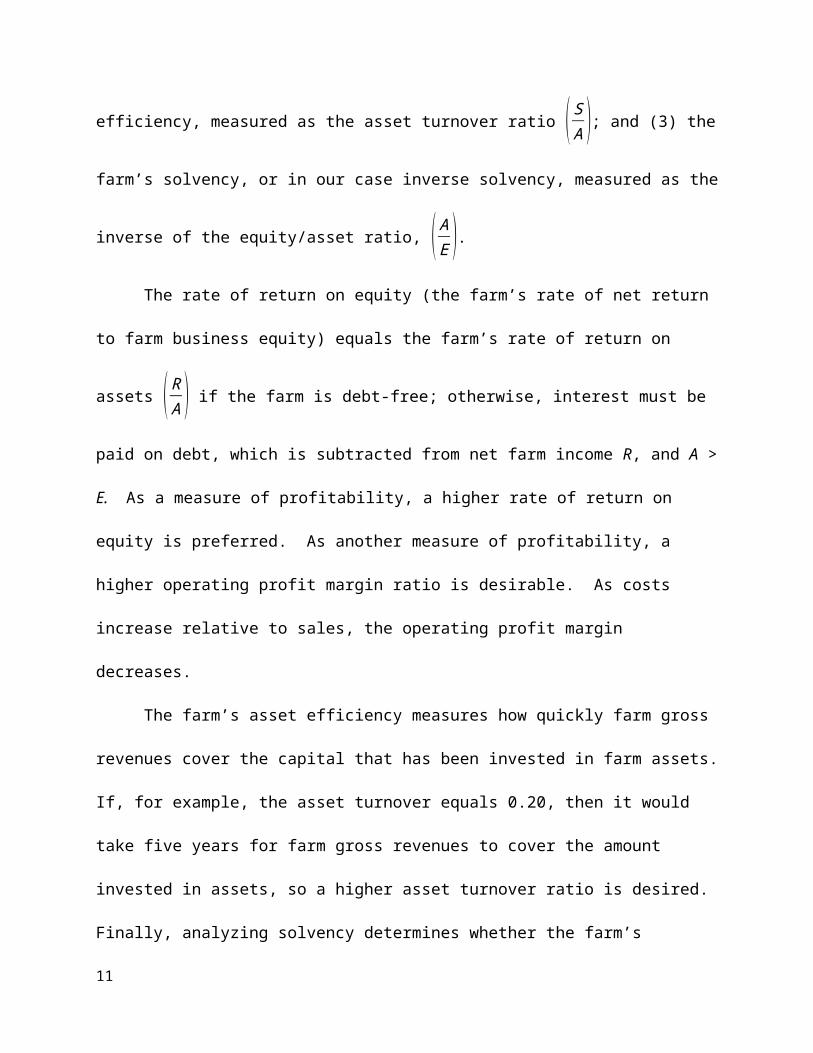
of (1) the farm’s profitability, measured by the operating profit margin ratio( RS ); (2) the farm’s

asset efficiency, measured as the asset turnover ratio ( SA ); and (3) the farm’s solvency, or in our

case inverse solvency, measured as the inverse of the equity/asset ratio, ( AE ).

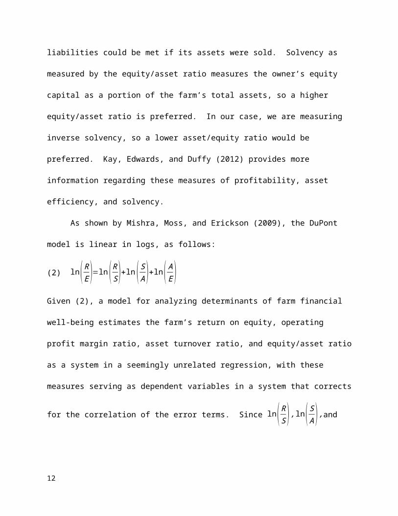
The rate of return on equity (the farm’s rate of net return to farm business equity) equals

the farm’s rate of return on assets ( RA ) if the farm is debt-free; otherwise, interest must be paid

on debt, which is subtracted from net farm income R, and A > E. As a measure of profitability, a

higher rate of return on equity is preferred. As another measure of profitability, a higher

operating profit margin ratio is desirable. As costs increase relative to sales, the operating profit

margin decreases.

The farm’s asset efficiency measures how quickly farm gross revenues cover the capital

that has been invested in farm assets. If, for example, the asset turnover equals 0.20, then it

would take five years for farm gross revenues to cover the amount invested in assets, so a higher

asset turnover ratio is desired. Finally, analyzing solvency determines whether the farm’s

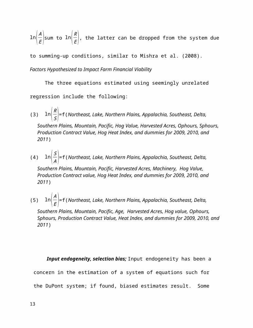
liabilities could be met if its assets were sold. Solvency as measured by the equity/asset ratio

measures the owner’s equity capital as a portion of the farm’s total assets, so a higher

equity/asset ratio is preferred. In our case, we are measuring inverse solvency, so a lower

7

asset/equity ratio would be preferred. Kay, Edwards, and Duffy (2012) provides more

information regarding these measures of profitability, asset efficiency, and solvency.

As shown by Mishra, Moss, and Erickson (2009), the DuPont model is linear in logs, as

follows:

(2) ln (RE )=ln (R

S )+ln( SA )+ ln( A

E )Given (2), a model for analyzing determinants of farm financial well-being estimates the farm’s

return on equity, operating profit margin ratio, asset turnover ratio, and equity/asset ratio as a

system in a seemingly unrelated regression, with these measures serving as dependent variables

in a system that corrects for the correlation of the error terms. Since ln ( RS ) , ln( S

A ) ,and ln ( AE )

sum to ln ( RE ), the latter can be dropped from the system due to summing-up conditions, similar

to Mishra et al. (2008).

Factors Hypothesized to Impact Farm Financial Viability

The three equations estimated using seemingly unrelated regression include the

following:

(3) ln (RS )=f(Northeast, Lake, Northern Plains, Appalachia, Southeast, Delta, Southern Plains,

Mountain, Pacific, Hog Value, Harvested Acres, Ophours, Sphours, Production Contract Value, Hog Heat Index, and dummies for 2009, 2010, and 2011)

(4) ln ( SA )=f(Northeast, Lake, Northern Plains, Appalachia, Southeast, Delta, Southern Plains,

Mountain, Pacific, Harvested Acres, Machinery, Hog Value, Production Contract value, Hog Heat Index, and dummies for 2009, 2010, and 2011)

(5) ln ( AE )=f(Northeast, Lake, Northern Plains, Appalachia, Southeast, Delta, Southern Plains,

Mountain, Pacific, Age, Harvested Acres, Hog value, Ophours, Sphours, Production Contract Value, Heat Index, and dummies for 2009, 2010, and 2011)

8

Input endogeneity, selection bias; Input endogeneity has been a concern in the

estimation of a system of equations such for the DuPont system; if found, biased estimates

result. Some studies have used instrumental variables to correct the problem, while others

have argued either that (1) it was not problematic in their studies because random

disturbances in production processes resulted in proportional changes in the use of all inputs

(Coelli and Perelman 2000, Rodriguez-Alvarez 2007) or (2) no good instrumental variables

existed, thus endogeneity was not accounted for (Fleming and Lien 2010). We estimate

instruments for each of the off farm labor inputs. The Hausman test was used to test for

endogeneity. Since endogeneity was found, the predicted values are used as instruments in

the SUR.

In addition to endogeneity concerns associated with SUR inputs, selection bias may be

of concern. Since contractee producers self-select into contracts, they may have been more

or less productive than independent hog farmers regardless of whether or not they had opted

to produce hogs using a production contract. We correct for selection bias in our SUR

estimates. Examining the dairy sector Mayen et al. (2010) corrected for organic dairy

selection bias by using propensity score matching, while McBride and Greene (2009)

corrected for it by estimating the inverse Mills ratio in a first-stage probit equation and

including it in a second-stage profit equation. Our probit selection equation predicts the

probability of production contract hog production (in the Phase III data). The inverse Mills

ratio was significant in the profitability and efficiency equations in the SUR, suggesting

selection bias. Thus, it was included in the SUR as a correction for contract selection bias.

9

Using ARMS Data to Estimate a SUR

Since complex stratified sampling is used with ARMS, inferences regarding variable

means for regions are conducted using weighted observations. As discussed by Banerjee et

al. (2010), the ARMS is a multiphase, non-random survey, so classical statistical methods

may yield naïve standard errors, causing them to be invalid. Each observation represents a

number of similar farms based upon farm size and land use, which allows for a survey

expansion factor or survey weight, effectively the inverse of the probability that the surveyed

farm would be selected for the survey. As such, USDA-NASS has an in-house jackknifing

procedure that it recommends when analyzing ARMS data (Cohen et al. 1988; Dubman

2000; Kott 2005), which allows for valid inferences to the population. Thus, econometric

estimation of SUR models presents unique challenges when using ARMS data. We use the

jackknife replicate weights in SAS to obtain adjusted standard errors. A property of the

delete-a-group jackknife procedure is that it is robust to unspecified heteroscedasticity.

The USDA version of the delete-a-group jackknife ARMS survey design divides the

sample into 30 nearly equal and mutually exclusive parts. Thirty estimates of the statistic

(replicates) are created. One of the 30 parts is eliminated in turn for each replicate estimate

with replacement. The replicate and the full sample estimates are placed into the jackknife

formula:

(2) Standard Error (β) = ¿¿

where β is the full sample vector of coefficients from the SUR program results using the

replicated data for the “base” run. βk is one of the 30 vectors of regression coefficients for

each of the jackknife samples. The t-statistics for each coefficient are computed by dividing

the “base” run vector of coefficients by the vector of standard errors of the coefficients.

10

Model Results

Results of the probit model explaining grouping in production contracts and independent

operations are shown in the table below. These results are used to compute the inverse-Mills

ratios in the SUR estimates. The model is significant and correctly predicts 36 percent of those

farms that are production contract operations and of those hog operations that are independent

more than 97% are correctly predicted. We achieve good results in the sense that more than

half of the coefficients of the probit model are significant and the covariate is good at

distinguishing contractees from independent operations.

The SUR model was estimated using the DuPont inverse solvency, profitability, and

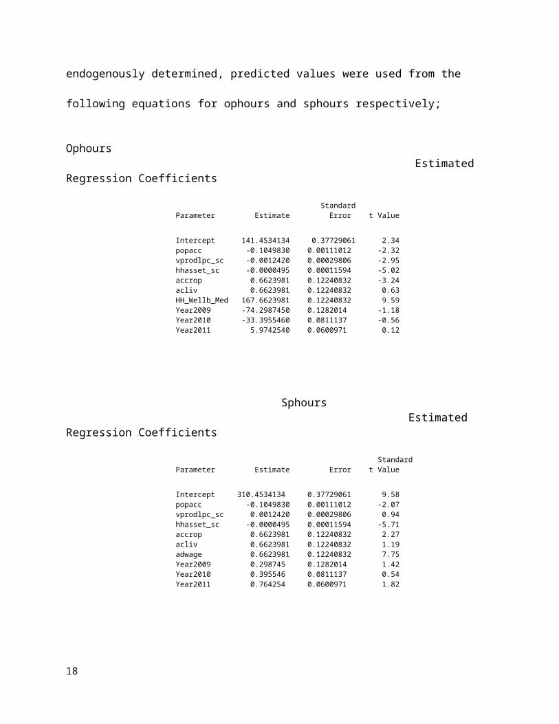
efficiency equations as defined above. The results are reported below. Because ophours and

sphours used in the inverse solvency equation are likely endogenously determined, predicted

values were used from the following equations for ophours and sphours respectively;

Ophours Estimated Regression Coefficients Standard Parameter Estimate Error t Value Intercept 141.4534134 0.37729061 2.34 popacc -0.1049830 0.00111012 -2.32 vprodlpc_sc -0.0012420 0.00029806 -2.95 hhasset_sc -0.0000495 0.00011594 -5.02 accrop 0.6623981 0.12240832 -3.24 acliv 0.6623981 0.12240832 0.63 HH_Wellb_Med 167.6623981 0.12240832 9.59 Year2009 -74.2987450 0.1282014 -1.18 Year2010 -33.3955460 0.0811137 -0.56 Year2011 5.9742540 0.0600971 0.12

Sphours Estimated Regression Coefficients Standard Parameter Estimate Error t Value Intercept 310.4534134 0.37729061 9.58 popacc -0.1049830 0.00111012 -2.07

11

vprodlpc_sc 0.0012420 0.00029806 0.94 hhasset_sc -0.0000495 0.00011594 -5.71 accrop 0.6623981 0.12240832 2.27 acliv 0.6623981 0.12240832 1.19 adwage 0.6623981 0.12240832 7.75 Year2009 0.298745 0.1282014 1.42 Year2010 0.395546 0.0811137 0.54 Year2011 0.764254 0.0600971 1.82

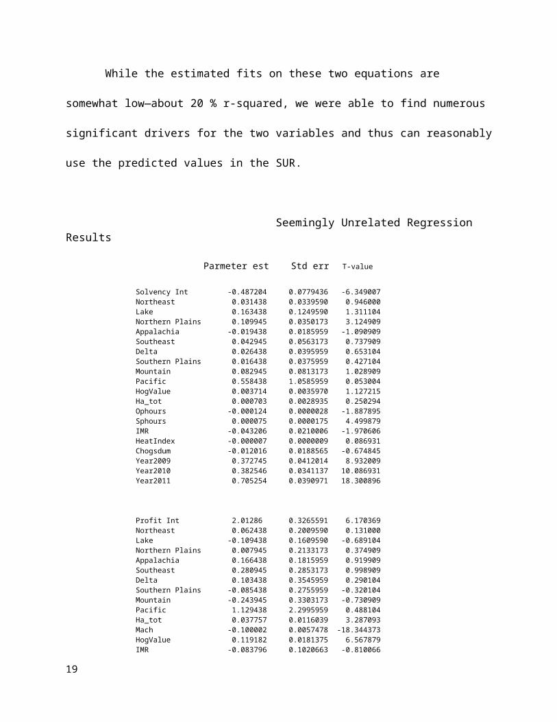
While the estimated fits on these two equations are somewhat low—about 20 % r-squared,

we were able to find numerous significant drivers for the two variables and thus can reasonably

use the predicted values in the SUR.

Seemingly Unrelated Regression Results Parmeter est Std err T-value Solvency Int -0.487204 0.0779436 -6.349007 Northeast 0.031438 0.0339590 0.946000 Lake 0.163438 0.1249590 1.311104 Northern Plains 0.109945 0.0350173 3.124909 Appalachia -0.019438 0.0185959 -1.090909 Southeast 0.042945 0.0563173 0.737909 Delta 0.026438 0.0395959 0.653104 Southern Plains 0.016438 0.0375959 0.427104 Mountain 0.082945 0.0813173 1.028909 Pacific 0.558438 1.0585959 0.053004 HogValue 0.003714 0.0035970 1.127215 Ha_tot 0.000703 0.0028935 0.250294 Ophours -0.000124 0.0000028 -1.887895 Sphours 0.000075 0.0000175 4.499879 IMR -0.043206 0.0210006 -1.970606 HeatIndex -0.000007 0.0000009 0.086931 Chogsdum -0.012016 0.0188565 -0.674845 Year2009 0.372745 0.0412014 8.932009 Year2010 0.382546 0.0341137 10.086931 Year2011 0.705254 0.0390971 18.300896 Profit Int 2.01286 0.3265591 6.170369 Northeast 0.062438 0.2009590 0.131000 Lake -0.109438 0.1609590 -0.689104 Northern Plains 0.007945 0.2133173 0.374909 Appalachia 0.166438 0.1815959 0.919909 Southeast 0.280945 0.2853173 0.998909 Delta 0.103438 0.3545959 0.290104 Southern Plains -0.085438 0.2755959 -0.320104 Mountain -0.243945 0.3303173 -0.730909 Pacific 1.129438 2.2995959 0.488104 Ha_tot 0.037757 0.0116039 3.287093 Mach -0.100002 0.0057478 -18.344373 HogValue 0.119182 0.0181375 6.567879 IMR -0.083796 0.1020663 -0.810066 Heat -0.000226 0.0000565 -2.528845 Chogsdum -0.237016 0.1418565 -1.683845 Popacc 0.000282 0.0001175 2.197879 Year2009 -0.043745 0.1290014 0.332009

12

Year2010 0.195546 0.1441137 1.346931 Year2011 0.441254 0.1269971 3.470896 Seemingly Unrelated Regression Results (Continued)

Efficiency Int -0.820451 0.4491188 -1.829731 Northeast 0.041438 0.1299590 0.319000 Lake -0.014238 0.1239590 -0.114104 Northern Plains 0.182945 0.1073173 1.694909 Appalachia -0.180438 0.1005959 -1.810909 Southeast -0.213945 0.2143173 -0.990909 Delta 0.117938 0.1275959 0.928104 Southern Plains -0.186438 0.1785959 -1.040104 Mountain -0.074945 0.1763173 -0.428909 Pacific 0.086438 0.6835959 0.124104 Age -0.734495 0.0983863 -7.432004 Ha_tot 0.017495 0.0053863 3.029004 Hogsvalue 0.220913 0.0165401 13.328873 Ophours -0.000129 0.0000163 -0.822866 Sphours -0.000087 0.0000727 -1.240772 IMR -0.016943 0.0711834 -0.237861 HeatIndex -0.000074 0.0000595 -1.406968 Chogsdum 0.292038 0.0919395 3.196968 Year2009 -0.391745 0.1122014 -3.482009 Year2010 -0.395546 0.0841137 -4.696931 Year2011 -0.728254 0.0700971 -10.030896

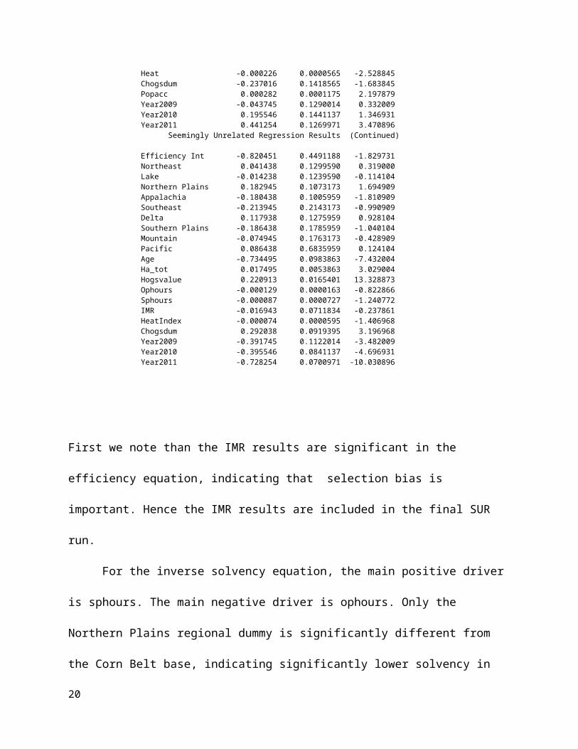
First we note than the IMR results are significant in the efficiency equation, indicating that

selection bias is important. Hence the IMR results are included in the final SUR run.

For the inverse solvency equation, the main positive driver is sphours. The main negative

driver is ophours. Only the Northern Plains regional dummy is significantly different from the

Corn Belt base, indicating significantly lower solvency in the Northern Plains compared to the

Corn Belt. All of the time dummies are significant indicating lower solvency over time.

For the profitability equation we find that the main positive drivers are acres harvested,

contract production, and value of hogs. The main negative drivers are machinery, a dummy for

Chogs=0, the hog heat index. Only the Southern Plains regional dummy is significantly different

from the Corn Belt base, indicating significantly lower profitability in the Southern Plains

compared to the Corn Belt. Only the 2011 time dummy is significant, indicating higher

profitability over time. The negative sign on chogsdum and its marginal significance indicates

that independent operations as a group tend to reduce profitability.

13

For the efficiency equation we find that the main positive drivers are acres harvested, value of

hogs, and a dummy for CHogs=0. The main negative drivers are age and the hog heat index.

The Northern Plains, Appalachia, Southeast, and Southern Plains regional dummies are

significantly different from the Corn Belt base, indicating large regional variation in efficiency.

All of the time dummies are significant and negative, indicating lower efficiency over time. The

positive sign on chogsdum and its significance indicates that independent operations as a group

boost efficiency.

Conclusions:

Based on the 2008-11 ARMS phase III data contractee hog operations in Iowa/Minnesota

and the Northern Plains, exhibited returns on equity of 9.7 and 9.2 percent, respectively, as

shown in Appendix Table 1, significantly higher than equity returns calculated for all other

contractee and independent regional groupings. The main drivers for this performance appear to

be high volume hog production (with inventories averaging close to 3,000 hogs per farm—see

Key and McBride 2013 on scale economies) coupled with relatively high corn yields (consistent

with high value land with little urban influence), and limited reliance on off-farm labor. Thus,

contractee groups showed the highest returns on equity. Some independent producers, however,

appear to be competitive. Among the important producing regions shown in Appendix Table 1,

for example, independent producers in Iowa/Minnesota exhibited competitive returns on equity

of 7.5 percent, followed by independent producers in the Southeast with 6.9 percent returns. In

contrast, return on equity was only 5.4 percent among contractee producers in Appalachia.

Looking at traditional financial measures, we find differences in returns on farm assets or

household assets between independent and contractee hog producers, generally, but not always

favoring contractee operations in the Phase III analysis. In particular, we find that traditional

14

household financial returns among independents in Iowa/Minnesota-and the Northern Plains are

competitive with contractee returns in Appalachia. And return on equity derived from the

DuPont measures in these groupings are competitive with return on equity among Appalachia

contractee producers.

It is useful to compare these Phase III results to those for the population estimates in 2009.

First, we see that contractees show higher returns on assets and household returns as shown in

Appendix Table 2. Among the DuPont measures shown in Appendix 2 we find that contractees

are less efficient than independents, have the same solvency, but higher profitability, and higher

returns on equity. But comparing contractees in the East, including North Carolina, with

independent producers in the West, we find no difference in household returns. Among the

DuPont measures, we find that contractees in the East have significantly lower solvency and

efficiency ratios (as reflected in the positive coefficient on chogsdum in the SUR efficiency

results) and higher profitability (as reflected in the negative coefficient on the chogsdum in the

SUR profitability results) compared with independent operations in the West. And, they have

comparable returns on equity compared with independents in the West. In summary these Phase

III and COP results indicate that some independent hog producers remain competitive,

suggesting the rate of sharp decline in independent hog production that took place between 1992

and 2004 may have slowed. In future research we will sort on DuPont results more thoroughly to

account for differences in organizational arrangement—whether farrowing or not---as production

contracts tend to be much more prevalent on finish operations.

References

Collins, Robert A., “Expected Utility, Debt-Equity Structure, and Risk Balancing,” American Journal of Agricultural Economics, volume 3, number 3, August 1985, pp. 627-29.

15

Gillespie, J., and A. Mishra. “Off-farm Employment and Reasons for Entering Farming as Determinants of Production Enterprise Selection in U.S. Agriculture.” Australian Journal of Agricultural and Resource Economics 55,3(2011):411-428.

Key, Nigel and McBride, W.D., “Trends and Developments in U.S. Hog Production 1992 to 2009: Technology, Reorganization, and Productivity Growth. ” Economic Research Report No. __, USDA-Economic Research Service, Forthcoming 2013.

Key, Nigel and McBride, W.D., “The Changing Economics of U.S. Hog Productions.” Economic Research Report No. 52, USDA-Economic Research Service, December 2007.

Key, Nigel “Production Contracts and Farm Business Growth and Survival.” Journal of Agricultural and Applied Economics Forthcoming.

Mishra, A.K., J.M. Harris, K. Erickson, and C. Hallahan. “What Drives Agricultural Profitability in the U.S.: Application of the DuPont Expansion Method.” Selected paper presented at the annual meetings of the American Agricultural Economics Association, July 27-29, 2008, Orlando, FL.

Mishra, A.K., C.B. Moss, and K.W. Erickson. “Regional Differences in Agricultural Profitability, Government Payments, and Farmland Values: Implications of DuPont Expansion.” Agricultural Finance Review 69,1(2009):49-66.

PRISM Group. 2008. Gridded climate data time series for the conterminous United States, 1895-2008. Oregon State University. http://prism.oregonstate.edu.

U.S. Department of Agricultural, National Agricultural Statistics Service. Agricultural Statistics, 2005. U.S. Government Printing Office, Washington, DC, 2005.

U.S. Department of Agricultural, National Agricultural Statistics Service. Agricultural Statistics, 2009. U.S. Government Printing Office, Washington, DC, 2009.

U.S. Department of Agricultural, National Agricultural Statistics Service. Agricultural Statistics, 2010. U.S. Government Printing Office, Washington, DC, 2010.

16

Figure 1: Heat Index for Hogs

17

0102030405060708090

Northeast

LakeStates

CornBelt

NorthPlains

App Southeast

Delta SouthPlains

Moutain Pacific

contractslvstk prod

Red: Contracts Blue; livestock prod

Source; Phase III ARMS 2008-2011 and COP ARMs 2009

Percent of production

Chart 1: Production Contracts as percent of Production by Region; over 50 percent in Regions accounting for 72

percent of hog production

18

Source: Prism and GIS/ERS calculations

1. Appendix table 1 Economic and Technical Data: Means and Statistics by Independent Compared to Contractee Operations

in all States 2008-2011

Item App

Ind

App

Cont

CB

Ind

CB

Cont

IAMN

Ind

IAMN

Cont

NP

Ind

NP

Cont

SE

Ind

SE

Cont

West

Ind

Number of Observations

936 909 1,776 509 819 695 820 105 1,503 199 1,305

Percent of Farms

20.0 0.9 18.5 1.1 5.4 2.2 5.5 0.4 26.0 0.2 19.9

Value of Production (%)**

5.0 10.5 10.2 9.3 10.4 23.8 10.7 3.0 8.2 1.6 7.3

Hogs per farm

23 5,362 145 2,218 641 3,921 390 2,646 350 2,467 21

Acres op 97 421 155 572 344 682 1,345 704 550 489 592

Popacc

(urbanization)

307 214 188 120 71 54 46 40 137 53 172

Corn yield (bu/ac)

125 106 155 65 169 175 141 164 98 158 167

Land price ($/acre)

2,833 2,511 2,483 2,573 2,943 3,441 680 2,264 894 849 843

19

17

Item App

Ind

App

Cont

CB

Ind

CB

Cont

IAMN

Ind

IAMN

Cont

NP

Ind

NP

Cont

SE

Ind

SE

Cont

West

Ind

Off-farm income (%)

71.1 6.2 34.6 5.3 9.3 5.0 15.7 4.2 61.0 3.4 57.8

Return on Assets (%)

1.1 5.7 3.2 6.6 8.2 9.8 5.1 9.8 0.7 10.0 1.7

Household return (%)

6.5 5.1 6.8 7.3 8.9 9.5 6.3 11.8 5.7 7.9 4.7

Solvency 78.0 86.1 82.2 91.0 87.3 94.9 86.7 94.0 79.2 82.8 80.2

Profitability 8.5 24.8 14.2 19.1 20.7 27.0 17.7 22.3 8.1 25.7 13.9

Efficiency 13.8 25.2 24.1 37.1 41.3 38.0 29.0 44.1 10.8 39.8 12.6

Return on Equity

0.9 5.4 2.8 6.4 7.5 9.7 4.5 9.2 6.9 8.5 1.4

** Percent of production on hogs only for production contract is 40 percent.

Source: 2008-2011 ARMS Phase III.

20

Appendix table 2 Economic and Technical Data: Means and Statistics by Independent Compared to Contractee Operations in all States 2009

Item All

Independent

All

Contract

West

Independent

West

Contract

East

Independent

East

Contract

Number of Observations

549 737 443 408 106 329

Percent of Farms

49 51 44 42 5 10

Value of Production (%)

28 72 27.5 55.1 1.0 16.5

Hogs per farm

1,476 3,571 1,577 3,202 519 5,124

Acres op 747 582 794 631 303 372

Popacc

(urbanization)

111 83 99 66 223 152

Corn yield (bu/ac)

173 177 174 180 142 115

21 17

Land price ($/acre)

1,499 1,863 1,440 1,866 2,961 1,851

Item All

Independent

All

Contract

West

Independent

West

Contract

East

Independent

East

Contract

Off-farm income (%)

2.8 2.9 2.7 2.7 7.0 4.2

Return on Assets (%)

3.7 9.6 3.8 10.3 2.2 6.3

Household return (%)

4.7 8.1 4.8 8.8 3.2 4.8

Solvency 87.9 88.6 88.8 90.6 76.5 80.5

Profitability 8.7 25.0 8.6 25.3 11.5 23.3

Efficiency 42.6 38.4 44.3 40.8 18.9 27.2

Return on Equity

3.0 8.4 3.1 9.4 1.7 5.1

Source: 2009 ARMS COP.

22

Appendix table 3 Economic and Technical Data: Means and Statistics by Region in all states 2008-2011 and 2009

Item NorthEast

LakeStates

CCorn Belt

NNNorthPlains

App Southeast

Delta SouthPlains

Mount Pacific

Prod cont (%) of prod

49.0 64.0 71.0 26.0 88.0 26.0 27.0 29.0 12.0 0.0

Number of Observations

428 1,112 2,687 925 1,417 505 430 767 527 783

Percent of Farms

8.9 8.1 18.1 5.9 12.2 7.1 4.0 15.6 11.0 9.2

Value of Production (%)

3.6 12.0 41.0 13.6 11.6 2.4 3.1 3.9 5.8 3.0

Value of Production (%) 2009

1.5 14.8 52.6 11.0 14.9 ---- 0.6 3.0 --- ---

Hogs per farm 2009

1,562 2,119 2,725 2,212 4,955 --- 999 2,016 ---- -----

Acres op 96 226 291 1,362 122 95 154 868 967 206

Popacc 505 134 147 44 171 163 94 137 75 206

Land price ($/acre)

3,447 2,299 3,005 729 2,487 2,435 1,452 793 574 2,277

23

Item NorthEast

LakeStates

CCorn Belt

NNNorthPlains

App Southeast

Delta SouthPlains

Mount Pacific

Off farm income (%)

55.3 15.7 16.3 13.2 60.8 59.8 43.0 63.4 50.9 58.9

Corn yield (bu/arac)

133 165 168 144 100 107 122 85 164 199

Solvency 82.2 85.6 87.6 87.3 76.9 74.2 75.8 81.3 79.4 81.8

Profitability 14.4 20.9 20.4 19.1 9.6 5.0 25.1 2.7 12.4 13.3

Efficiency 16.3 39.1 31.6 30.6 15.1 13.3 30.0 7.8 14.9 11.3

Return on Equity

1.9 7.0 5.6 5.1 1.1 0.5 5.7 0.2 1.5 1.2

Source: 2008-2011 ARMS Phase III.

24