Note: This chapter was totally reviewed. This is a first draft, as preliminary information. Another more advanced draft is expected to be provided by the time of the CIMO Guide Editorial Board meeting (13-15 Nov. 2013).

RADAR MEASUREMENTS

REVISION 2P

9.1 GENERAL

This chapter is a basic discussion of meteorological weather radars. It places particular emphasis on the technical and operational characteristics that must be considered when planning, developing and operating individual radars and radar networks in support of Meteorological and Hydrological Services. This is related to the use and applica -tion of weather radar data. Radars used for vertical wind profiling are discussed in Part II, Chapter 5.

9.1.1 The Weather Radar

Meteorological radars are primarily designed for detecting precipitation and associated phenomena. However, other objects such as insects, birds, planes, sand and dust, ground clutter and even fluctuations in the refractive index in the atmosphere generated by local variations in temperature or humidity can be detected by the weather radar.

This chapter deals with radars in common operational or near-operational use around the world. The meteorological radars having characteristics best suited for atmospheric observation and investigation transmit electromagnetic pulses in the 3–10 GHz frequency range (10–3 cm wavelength, respectively). Primarily, they are designed for detect-ing and mapping areas of precipitation, measuring their intensity and motion, and their type. Birds, insects ant the turbulent fluctuations can also produce using wind information with Doppler radar. Their intensity patterns can re -veal the location of atmospheric boundaries that are indicative of areas of low level convergence where thunder -storms may initiate or develop.

Higher frequencies (35 and 94 GHz) are used to detect smaller hydrometeors, such as cloud, fog, drizzle, snow and light precipitation are becoming prevalent in the research community. These frequencies are generally not used in operational forecasting for precipitation detection or general weather surveillance because of excessive attenuation of the radar signal by the intervening medium and their relatively short range, particularly, in Doppler mode.

At lower frequencies (915-1440Mhz, ~400-440 Mhz and ~50MHz), radars are capable of detecting variations in the refractive index of clear air, and they are used for wind profiling. Although they may detect precipitation, their scan -ning capabilities are limited by the size and type of the antenna that generally point in the vertical.

The returned signal from the transmitted pulse encountering any target, called an echo, has an amplitude, a phase and a polarization. Most operational radars worldwide are still limited to analysis of the amplitude feature that is re -lated to the size distribution and numbers of particles in the (pulse) volume illuminated by the radar beam. The am -plitude is used to determine the reflectivity factor (Z) to estimate the mass of precipitation per unit volume or the in-tensity of precipitation through the use of empirical relations. A primary application is thus to detect, map and esti -mate the precipitation at ground level instantaneously, nearly continuously and over large areas.

Doppler radars have the capability of determining the phase difference between the transmitted and received pulse and is a measure of the mean radial velocity of the particles. This is the reflectivity weighted average of the radial components of the displacement velocities of the hydrometeors within the pulse volume. The Doppler spectrum width is a measurement of the spatial variability of the Doppler velocities and provides a measure of the wind shear and turbulence. Virtually all currently commercially available weather radars have Doppler capability. An important feature of Doppler is the ability to filter out echoes due to ground targets in the signal processing.

The current generation of radars have polarization capability. Operationally, pulses are transmitted simultaneously with horizontal and vertical polarizations. In the past, the pulses were transmitted in sequence but required a high power polarization switch that was prone to failure. Two receivers (physical or virtual) are used to measure the hori -zontal and vertical components of the returned signal. The main benefits are improved data quality through the abil -ity to identify characteristics of the target (birds, bugs, precipitation and its type, clutter). For forecast applica=tions, the dual-polarization capability can identify hail and the rain-snow boundary. In addition, high precipitation rates af -fect the horizontal and vertical phase of the transmitted and received pulses. This can be exploited for precipitation estimation even with partially blocked beams or uncalibrated power calibration.

Weather radars do not operate in isolation. Given current telecommunication capabilities, data are exchanged re-sulting in networks of weather radar and extend its use from local application (e.g. severe weather warnings and

nowcasting) to regional (e.g. data assimilation, precipitation estimation) and global application (e.g. climate change detection).

Modern weather radars should have characteristics optimized to produce the best data for operational requirements. They are the most complex of all the weather sensors used in operations and require special training and extensive knowledge of the instrument. The location of the radar is critical to meet the surveillance and detection require-ments. There are a variety of configuration options to set up the radar. Components should be adequately installed and monitored for degradation and failure. Hence, a maintenance and support program is needed to keep this in -strument useful.

9.1.2 Radar characteristics, terms and units

The meteorological applications govern the selection of the characteristics of the radar. (Tables 9.1, 9.2 and 9.3).

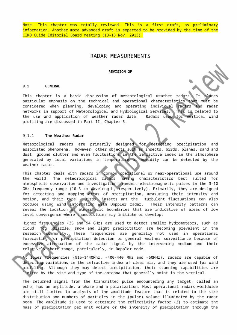
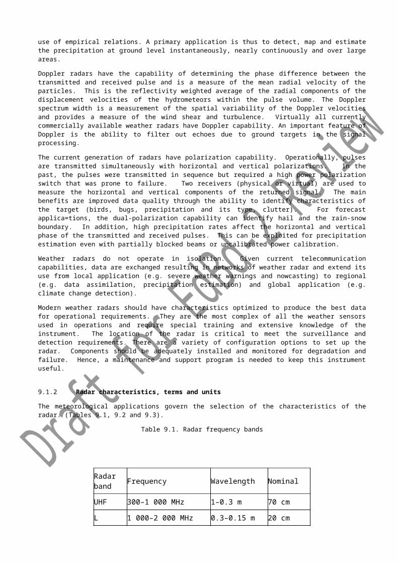
Table 9.1. Radar frequency bands

Radar band Frequency Wavelength Nominal

UHF 300–1 000 MHz 1–0.3 m 70 cm

L 1 000–2 000 MHz 0.3–0.15 m 20 cm

Sa 2 000–4 000 MHz 15–7.5 cm 10 cm

Ca 4 000–8 000 MHz 7.5–3.75 cm 5 cm

Xa 8 000–12 500 MHz 3.75–2.4 cm 3 cm

Ku 12.5–18 GHz 2.4–1.66 cm 1.50 cm

K 18–26.5 GHz 1.66–1.13 cm 1.25 cm

Ka 26.5–40 GHz 1.13–0.75 cm 0.86 cm

W 94 GHz 0.30 cm 0.30 cm

a Most common weather radar bands.

Table 9.2. Some meteorological radar parameters and units

Symbol Parameter Units

Ze Equivalent or effective radar reflectivity mm6 m–3 or dBZ

Vr Mean radial velocity m s–1

σv Spectrum width m s–1

Zdr Differential reflectivity dB

CDR Circular depolarization ratio dB

LDR Linear depolarization ratio dB

kdp Propagation phase Degree km–1

ρ Correlation coefficient

Table 9.3. Physical radar parameters and units

Symbol Parameter Units

9.1.3 Radar accuracy requirements

Quantitative use of the radar data in end-user applications rely on the accuracy and precision of the radar observa -tions. Appropriately installed, calibrated and maintained modern radars are relatively stable and do not produce sig-nificant measurement errors. Radar is probably the most complex of weather sensors used operationally and main-tenance anc calibration of the radar is still a considerable challenge and requires highly qualified personnel. Mea-surement bias still exists and requires engineering and scientific experience and expertise to monitor, diagnose and mitigate.

External physical factors, such as ground clutter effects, anomalous propagation, attenuation and propagation ef -fects, beam effects, target composition, particularly with variations and changes in the vertical, rain rate-reflectivity relationship inadequacies and the meteorological situation, create artifacts in the data that must be removed or tak -ing into account for use in quantitative applications.

By considering only errors attributable to the radar system, the measurable radar parameters can be determined with an acceptable accuracy (Table 9.4).

Table 9.4. Accuracy requirements

Parameter

Definition

Acceptable accuracy a

Azimuth angle

0.1˚

γ

Elevation angle

0.1˚

Vr

Mean Doppler velocity

0.5 m s–1

Z

Reflectivity factor

0.5 dBZ

σv

Doppler spectrum width

0.5 m s–1

Zdr

Kdp

LDR

a These figures are relative to a normal Gaussian spectrum with a standard deviation smaller than 4 m–1. Velocity accuracy deteriorates when the

spectrum width grows, while reflectivity accuracy improves.

9.2 RADAR PRINCIPLES

9.2.1 Pulse Radars

The principles of radar and the observation of weather phenomena were established in the 1940s. Since that time, great strides have been made in improving equipment, signal and data processing and its interpretation. The inter -ested reader should consult some of the relevant texts for greater detail. Good references include Skolnik (1970) for engineering and equipment aspects; Battan (1981) for meteorological phenomena and applications; Atlas (1964; 1990), Sauvageot (1982) and WMO (1985) for a general review; Rinehart (1991???) for a meteorologists perspec -tive; Doviak and Zrnic (1993) for Doppler radar principles and applications, Bringi and Chandrasekar (???) and Meis-chner (???) for dual-polarization. Considerable insight on radar quality, maintenance, hardware monitoring and cali -bration can be gleaned from the RADCAL 2000 workshop (ref.), RADCAL 2013 (???) and the RADMON 2012 (??) workshops. A brief summary of the principles follows.

Meteorological radars used in operational networks are pulsed radars. Frequency modulated – continuous wave (FMCW) radars use modulated frequency (usually linear) within a very long pulse to determine range. High resolution can be achieved but has limited range and so not used for operational use. Electromagnetic waves at fixed preferred frequencies are transmitted from a directional antenna into the atmosphere in a rapid succession of short pulses. The pulse length and range processing determines the range resolution of the radar data. Leading edge operational radars are being deployed with low power transmitters (Solid State, Traveling Wave Tubes) that use a technique called pulse compression that use a combination of long pulses, frequency modulation and advanced signal processing to achieve high range resolution and high sensitivity that rival traditional pulse systems. Phased array antennae are an emerging technology that form the beam by electronic phase shifting. They have the ability to point to different locations in an agile and non-sequential fashion. However, they all use a directional beam that can resolve targets in range.

Fig. 9.1 shows a directional radar antenna emitting a pulsed-shaped beam of electromagnetic energy over the Earth’s curved surface and illuminating a portion of a meteorological target. Many of the physical limitations and constraints of the observation technique are immediately apparent from the figure. For example, there is a limit to the minimum altitude that can be observed at far ranges due to the curvature of the Earth.

A parabolic reflector in the antenna system concentrates the electromagnetic energy in a conical-shaped beam that is highly directional. The width of the beam increases with range, for example, a nominal 1° beam spreads to 0.9, 1.7 and 3.5 km at ranges of 50, 100, and 200 km, respectively.

The short bursts of electromagnetic energy are absorbed and scattered by meteorological and non-meteorological targets encountered. Some of the scattered energy is reflected back to the radar antenna and receiver. Since the electromagnetic wave travels with the speed of light (that is, 2.99 × 108 m s–1), by measuring the time between the transmission of the pulse and its return, the range of the target is determined. Between the transmission of succes -sive pulses, the receiver listens for any return of the wave. The return signal from the target is commonly referred to as the radar echo. The time between pulses determines the maximum unambiguous range of the radar. Echoes can still be received from echoes beyond this maximum range and are known as multiple trip echoes.

The strength of the signal reflected back to the radar receiver is a function of the concentration, size and water phase of the echoes that make up the target. The power return, Pr, therefore provides a measure of the characteris-tics of the target and is, but not uniquely, related to a precipitation rate depending on the form of precipitation. The “radar range equation” relates the power-return from the target to the radar characteristics and parameters of the tar-get (see below).

The power measurements are determined by the total power backscattered by the target within a volume being sam-pled at any one instant — the pulse volume (i.e. sample volume). The pulse volume dimensions (which determines the resolution of the radar) are dependent on the radar pulse length in space (h) and the antenna beam widths in the vertical (b) and the horizontal (θb). The beam width, and therefore the pulse volume, increases with range. Since the power that arrives back at the radar is involved in a two-way path, the pulse-volume length is only one half pulse length in space (h/2) and is invariant with range. The location of the pulse volume in space is determined by the po-sition of the antenna in azimuth, the elevation, the range to the target and also by the non-linear propagation path of the radar beam away from the radar. The range (r) is determined by the time required for the pulse to travel to the target and to be reflected back to the radar.

Particles within the pulse volume are continuously shuffling relative to one another. This results in phase effects in the scattered signal and in intensity fluctuations about the mean target intensity. Little significance can be attached to a single echo intensity measurement from a weather target. At least 25 to 30 pulses must be integrated to obtain a reasonable estimation of mean intensity (Smith, 1995). This was formerly carried out an electronic integrator circuit

but is now done in a digital signal processor. Further averaging of pulses in range, azimuth and time is often con -ducted to increase the sampling size and accuracy of the estimate. It follows that the space resolution is coarser. An important difference with non-meteorological radars is that the weather radar processing and the interpretation of the data is designed to detect the backscatter from a distributed target and not from a point target (such as a airplane). This requires processing for quantitative measurements (not just detection) and a different range dependency of the return power.

Doppler radars have circuitry to measure the phase shift difference from successive pulses from the same radar pulse volume. The frequency shift within a pulse volume, which is the true Doppler shift, is not possible to be mea-sured using current technology. The phase shift is proportional of the radar wavelength and therefore distance in the time between pulses. This is the Doppler velocity.

Dual-polarization radar can be of several types. The polarization can be circular and though there have been very excellent research radars with this feature, it is not generally used in weather operations. Linear dual-polarization can sent pulses at horizontal and vertical polarization in alternating or simultaneous fashion. In the former case, a fast high power switch (switches every pulse) is required that has proved to be problematic and so few exist in oper-ations. The simultaneous transmission and receive transmits (commonly known as STAR mode) essentially trans -mits at a 45o angle and the signal is received at horizontal and vertical polarizations. This has proved to be the solu -tion for operations as the high power high failure fast switch is avoided. There are variations to these various meth-ods of creating the dual-polarization signal. The major advantage of the alternating dual-polarization mode is that it can measure the cross-polarization backscatter of the target (Linear Depolarization Ratio - LDR) and this is very useful for bright band detection. The major disadvantage of the STAR mode is the loss of LDR (there is cross-polar -ization already in the transmitted pulse) and the loss of 3dB of sensitivity (due to power splitting). The loss of LDR is partially compensated with use of other dual-polarization parameters.

9.2.2 PROPAGATION RADAR SIGNALS

Electromagnetic waves propagate in straight lines, in a homogeneous medium, at the speed of light. However, the atmosphere is vertically stratified and the rays change direction depending on the changes in the refractive index (or temperature and moisture). When the waves encounter precipitation and clouds, part of the energy is absorbed and a part is scattered in all directions or back to the radar site.

The amount of bending of electromagnetic waves can be predicted by using the vertical profile of temperature and moisture (Bean and Dutton, 1966). Under normal atmospheric conditions, the waves travel in a curve bending slightly earthward. In the standard propagation model, the beam propagates in a prescribed fashion. If the Earth is assumed to a have a radius of four thirds (4/3) of its actual radius, the beam propagates in a straight line. This is most often used but some radars (mountain top) use a five fourths (5/4) model (Fig. 9.x). The height about the radar is given by the following equation:

h = [ r2 + (kea) 2 + 2rkea sin e]1/2 - kea

where h is height above the radar antenna, r is the range along the beam, a is the Earth’s radius, e is the elevation angle above the horizon and kea is the effective Earth’s radius.

The ray path can bend either upwards (sub-refraction) or more earthward (super-refraction). In either case, the alti-tude of the beam will be in error using the standard atmosphere assumption. This is known as anomalous propaga -tion (AP or ANAPROP). From a direct precipitation measurement standpoint, the greatest problem occurs under su -per-refractive or “ducting” conditions. The ray can bend sufficiently to strike the Earth and cause ground echoes not normally encountered. The phenomenon occurs when the index of refraction decreases rapidly with height, for ex -ample, an increase in temperature and a decrease in moisture with height. These echoes must be dealt with in pro -ducing a precipitation map. In the sub-refraction situation, where the beam doesn’t beam as much as normally or bends in the upward direction, it is not evident that this situation is occurring. In actual practice, the vertical profile of the index of refraction is not measured and so the precise location of the beam is known.

Some “clear air” echoes are due to turbulent inhomogeneities in the refractive index. This is found in areas of turbu -lence, in layers of enhanced stability, wind shear cells, or strong inversions. These echoes usually occur in patterns, mostly recognizable, but must be eliminated as precipitation fields (Gossard and Strauch, 1983).

9.2.3 Attenuation in the atmosphere

Microwaves are subject to attenuation owing to atmospheric gases, clouds and precipitation by absorption and scat -tering.

Attenuation by gases

Gases attenuate microwaves in the 3–10 cm bands. Absorption by atmospheric gases is due mainly to water vapour and oxygen molecules. Attenuation by water vapour is directly proportional to the pressure and absolute humidity and increases almost linearly with decreasing temperature. The concentration of oxygen, to altitudes of 20 km, is rel -atively uniform. Attenuation is also proportional to the square of the pressure.

Attenuation by gases varies slightly with the climate and the season. It is significant at weather radar wavelengths over the longer ranges and can amount to 2 to 3 dB at the longer wavelengths and 3 to 4 dB at the shorter wave -lengths, over a range of 200 km. Compensation can be quite easily accomplished automatically.

Attenuation by hydrometeors

Attenuation by hydrometeors can result from both absorption and scattering. It is the most significant source of atten-uation. It is dependent on the shape, size, number and composition of the particles. This dependence has made it very difficult to overcome in any quantitative way using radar observations alone. Progress in dual polarization techniques have shown great promise in compensating for attenuation and the situation is rapidly changing.

Attenuation is dependent on wavelength. At 10 cm wavelengths, the attenuation exists but is rather small, while at 3 cm it is quite significant. At 5 cm, the attenuation may be acceptable for many climates, particularly in the high mid-latitudes. Wavelengths below 5 cm are not recommended for good precipitation measurement except for short-range applications (Table 9.5). Total attenuation of the signal can occur at 3 and 5 cm. Interestingly, with dual polarization techniques, the smaller wavelengths are more sensitive to attenuation and so these techniques are ef-fective starting at lower precipitation rates.

Table 9.5. One-way attenuation relationships

Wavelength (cm)

Relation (dB km–1)

10

0.000 343 R0.97

5

0.00 18 R1.05

3.2

0.01 R1.21

After Burrows and Attwood (1949). One-way specific attenuations at 18˚C. R is in units of mm hr–1.

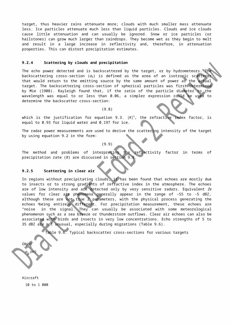
For precipitation estimates by radar, some general statements can be made with regard to the magnitude of attenua-tion. Attenuation is dependent on the water mass of the target, thus heavier rains attenuate more; clouds with much smaller mass attenuate less. Ice particles attenuate much less than liquid particles. Clouds and ice clouds cause lit -tle attenuation and can usually be ignored. Snow or ice particles (or hailstones) can grow much larger than rain -drops. They become wet as they begin to melt and result in a large increase in reflectivity and, therefore, in attenua -tion properties. This can distort precipitation estimates.

9.2.4 Scattering by clouds and precipitation

The echo power detected and is backscattered by the target, or by hydrometeors. The backscattering cross -section (σb) is defined as the area of an isotropic scatterer that would return to the emitting source by the same amount of power as the actual target. The backscattering cross-section of spherical particles was first determined by Mie (1908). Rayleigh found that, if the ratio of the particle diameter to the wavelength was equal to or less than 0.06, a

simpler expression could be used to determine the backscatter cross-section:

(9.8)

which is the justification for equation 9.3. |K|2, the refractive index factor, is equal to 0.93 for liquid water and 0.197 for ice.

The radar power measurements are used to derive the scattering intensity of the target by using equation 9.2 in the form:

(9.9)

The method and problems of interpreting the reflectivity factor in terms of precipitation rate (R) are discussed in sec-tion 9.9.

9.2.5 Scattering in clear air

In regions without precipitating clouds, it has been found that echoes are mostly due to insects or to strong gradients of refractive index in the atmosphere. The echoes are of low intensity and are detected only by very sensitive radars. Equivalent Ze values for clear air phenomena generally appear in the range of –55 to -5 dBZ, although these are not true Z parameters, with the physical process generating the echoes being entirely different. For precipitation mea-surement, these echoes are “noise” in the signal. They can usually be associated with some meteorological phe -nomenon such as a sea breeze or thunderstorm outflows. Clear air echoes can also be associated with birds and in -sects in very low concentrations. Echo strengths of 5 to 35 dBZ are not unusual, especially during migrations (Table 9.6).

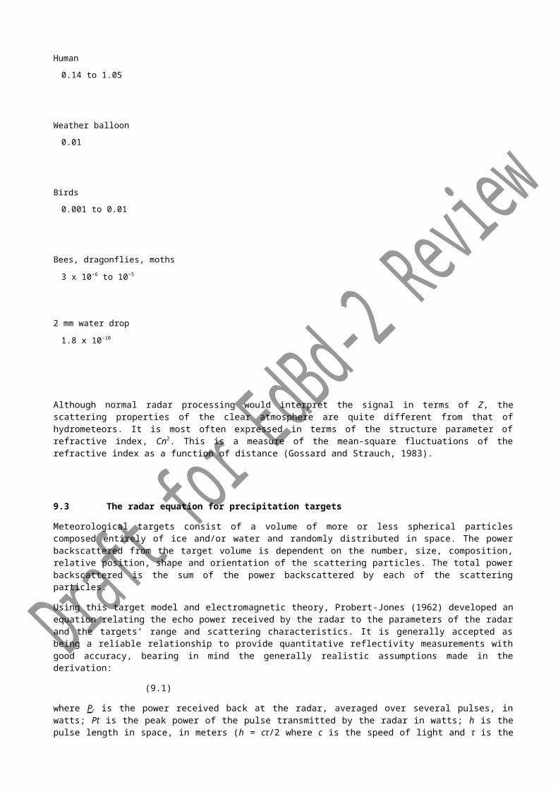
Table 9.6. Typical backscatter cross-sections for various targets

Object

σb (m2)

Aircraft

10 to 1 000

Human

0.14 to 1.05

Weather balloon

0.01

Birds

0.001 to 0.01

Bees, dragonflies, moths

3 x 10–6 to 10–5

2 mm water drop

1.8 x 10–10

Although normal radar processing would interpret the signal in terms of Z, the scattering properties of the clear atmosphere are quite different from that of hydrometeors. It is most often expressed in terms of the structure parameter of refractive index, Cn2. This is a measure of the mean-square fluctuations of the refractive index as a function of distance (Gossard and Strauch, 1983).

9.3 The radar equation for precipitation targets

Meteorological targets consist of a volume of more or less spherical particles composed entirely of ice and/or water and randomly distributed in space. The power backscattered from the target volume is dependent on the number, size, composition, relative position, shape and orientation of the scattering particles. The total power backscattered is the sum of the power backscattered by each of the scattering particles.

Using this target model and electromagnetic theory, Probert-Jones (1962) developed an equation relating the echo power received by the radar to the parameters of the radar and the targets’ range and scattering characteristics. It is generally accepted as being a reliable relationship to provide quantitative reflectivity measurements with good accuracy, bearing in mind the generally realistic assumptions made in the derivation:

(9.1)

where Pr is the power received back at the radar, averaged over several pulses, in watts; Pt is the peak power of the pulse transmitted by the radar in watts; h is the pulse length in space, in meters (h = cτ/2 where c is the speed of light and τ is the pulse duration); G is the gain of the antenna over an isotropic radiator; θb and b are the horizontal and vertical beam widths, respectively, of the antenna radiation pattern at the –3 dB level of one-way transmission, in radians; λ is the wavelength of the transmitted wave, in meters; |K|2 is the refractive index factor of the target; r is the slant range from the radar to the target, in meters; and Z is the radar reflectivity factor (usually taken as the equivalent reflectivity factor Ze when the target characteristics are not well known), in mm6 m–3.

The second term in the equation contains the radar parameters, and the third term the parameters depend on the range and characteristics of the target. The radar parameters, are relatively fixed, and, if the transmitter is operated and maintained at a constant output (as it should be), the equation can be simplified to:

(9.2)

where C is the radar constant.

There are a number of basic assumptions inherent in the development of the equation which have varying impor -tance in the application and interpretation of the results. Although they are reasonably realistic, the conditions are not always met exactly and, under particular conditions, will affect the measurements (Aoyagi and Kodaira, 1995). These assumptions are summarized as follows:(a) The scattering precipitation particles in the target volume are homogeneous dielectric spheres whose

diameters are small compared to the wavelength, that is D < 0.06 λ for strict application of Rayleigh scattering approximations;

(b) The pulse volume is completely filled with randomly scattered precipitation particles;(c) The reflectivity factor Z is uniform throughout the sampled pulse volume and constant during the sampling in-

terval;(d) The particles are all water drops or all ice particles, that is, all particles have the same refractive index factor |

K|2 and the power scattering by the particles is isotropic;(e) Multiple scattering (among particles) is negligible;(f) There is no attenuation in the intervening medium between the radar and the target volume;(g) The incident and backscattered waves are linearly co-polarized;(h) The main lobe of the antenna radiation pattern is Gaussian in shape;(i) The antenna is a parabolic reflector type of circular cross-section;(j) The gain of the antenna is known or can be calculated with sufficient accuracy;(k) The contribution of the side lobes to the received power is negligible;(l) Blockage of the transmitted signal by ground clutter in the beam is negligible;(m) The peak power transmitted (Pt) is the actual power transmitted at the antenna, that is, all wave guide losses,

and so on, and attenuation in the radar dome, are considered;(n) The average power measured (Pr) is averaged over a sufficient number of pulses or independent samples to

be representative of the average over the target pulse volume.

This simplified expression relates the echo power measured by the radar to the radar reflectivity factor Z, and related

to the rainfall rate. These factors and their relationship are crucial for interpreting the intensity of the target and esti -mating precipitation amounts from radar measurements. Despite the many assumptions, the expression provides a reasonable estimate of the target mass. This estimate can be improved by further consideration of factors in the as -sumptions.

9.4 Basic weather radar

The basic weather radar consists of the following:(a) A transmitter to produce power at microwave frequency and a modulator creates the pulses and pulse rates;(b) An antenna to focus the transmitted microwaves into a narrow beam and receive the returning power;(c) A receiver to detect, amplify and convert the microwave signal into a low frequency signal;(d) A processor to extract the desired information from the received signal; (e) A system to process the data and a system to visualize the information in an intelligible form.

Other components that maximize the radar capability are:(a) A processor to produce supplementary displays; (b) A recording system to archive the data for training, study and records.

A basic weather radar may be non-coherent (e.g. magnetron or power amplifier type transmitter), that is, the phase of successive transmitted pulses is random. Doppler measurements can be made if the phase of the transmitted pulse is measured and the signal processed with reference to this phase. This is known as a coherent-on-receive Doppler radar. A coherent on transmit radar (e.g. kystron, solid state or oscillator-amplifier type transmitter) trans -mits the same phase. Powers transmitted by a weather radar are typically several hundreds of kilowatts to a mega watt of peak power concentrated in a pulse of a microsecond in width, whereas the average power is typically a few hundred watts, equivalent to a typical light bulb. Current systems use computers for radar control, digital signal pro -cessing, recording, product displays and archiving.

9.4.1 Reflectivity

The power backscattered from a typical radar is of the order of 10–8 to 10–15 W, covering a range of about 70 dB from the strongest to weakest targets detectable. Compared to the transmit power, this is over 20 orders of magnitude smaller. To measure the weakest and strongest signals simultaneously, receivers with large dynamic ranges (> 90 dB) are required. In the past, logarithmic receivers were and are still used. However, modern operational radars with linear receivers with 90 dB dynamic range (and other sophisticated features) are commonly available (Heiss, McGrew and Sirmans, 1990; Keeler, Hwang and Loew, 1995).

Many pulses must be averaged in the processor to provide the required precision. This can be integrated in differ -ent ways, currently usually in a digital form, and must account for the receiver transfer function (namely, linear or log-arithmic). In practice, for a typical system, the signal at the antenna is received, amplified, averaged over many pulses, corrected for receiver transfer, and converted to a reflectivity factor Z using the radar constant (see equation 9.x, the radar equation).

The reflectivity factor is the most important parameter for radar interpretation. The factor derives from the Rayleigh scattering model and is defined theoretically as the sum of particle (drops) diameters to the sixth power in the sam-ple volume:

Z = ∑ vol N(D) D6 (9.3)

where the unit of Z is mm6 m–3. In many cases, the numbers of particles, composition and shape are not known and an equivalent or effective reflectivity factor Ze is defined. For example, snow and ice particles must refer to an equivalent Ze which represents Z, assuming the backscattering particles were all spherical drops.

Rainfall rate is given by

R = ∑ vol N(D) VT ρπ(D/6)3 (9.4)

However, N(D) is not known and empirical relationships are developed between Z and R are developed. The most famous relationship

being that commonly known as the Marshall-Palmer relationship. Note that it was published in Marshall-Gunn (1952).

Z = 200 R 1.6 (9.5)

In order to cover the range of values, a common practice is to work in a logarithmic scale or dBZ units which are nu-merically defined as dBZe = 10 log10 Ze.

Volumetric observations of the atmosphere are normally made by scanning the antenna at a fixed elevation angle and subsequently incrementing the elevation angle in steps at each revolution. An important consideration is the res-olution of the targets. Parabolic reflector antennas are used to focus the waves into a pencil shaped or gaussian shaped beam. Larger reflectors create narrower beams, greater resolution and sensitivity at increasing costs. The

beam width, often defined by the half power points is one half that at the axis, is dependent on the wavelength, and may be approximated by:

(9.4)

where the units of θe are degrees; and d is the antenna diameter in the same units as λ. Good weather radars have beam widths of 0.5 to 1°.

The useful range of weather radars is dependent on the application and nature of the weather. Depending on the time interval between pulses (characterized by the pulse repetition frequency, say 300 s-1), the maximum unambigu-ous range of the radar can be hundreds of kilometers (e.g., 500km). However, given the beam propagation and the curvature of the Earth, the beam and therefore the pulse volume is high and big (e.g., ?? km and ?? wide). The beam may overshoot the weather, the pulse volume may not be filled and the sensitivity of the radar may not be suf -ficient to measure the precipitation intensity accurately. However, if echoes are observed, they will indicate very in -tense and hazardous thunderstorms or weather. Typical weather radars operate with a maximum range of the order of 250 km. A beam at an elevation of 0.5° is at a height of 4?? km above the Earth’s surface and the beam width is of the order of 1.5 km or greater.

For good quantitative precipitation measurements, a 1o beam width radar has an effective range of about 80 km. The smaller beam width of the radar, the greater the effective range (e.g. 0.65o has an effective range of about 120 km). At longer ranges, the data must be extrapolated to the ground. The beam spreads and under-filling results in under reporting of the precipitation intensity. This is weather regime dependent and the results discussed are for mid latitudes.

9.4.2 Doppler radar

The development of Doppler weather radars and their introduction to weather surveillance provide a new dimension to the observations (Heiss, McGrew and Sirmans, 1990). Doppler radar provides a measure of the targets’ velocity along a radial from the radar. So it provides a measurement of the velocity component of the wind in the direction ei -ther towards or away from the radar. A further advantage of the Doppler technique is the greater effective sensitivity to low reflectivity targets near the radar noise level when the velocity field can be distinguished in a noisy Z field.

The typical speeds of meteorological targets is typically less than 50 m/s, except in the case of tornadoes. As dis -cussed earlier, pulse to pulse phase changes are used to estimate the Doppler velocity. If the phase changes by more than ±180°, the velocity estimate is ambiguous. In order to unambiguously and accurately measure the Doppler velocity of meteorological targets, the pulse repetition frequency must high (smaller time interval between pulses) such that the maximum unambiguous range is reduced from a typical reflectivity only radar. At higher speeds, additional processing steps are required to retrieve the correct velocity. The maximum unambiguous Doppler velocity depends on the radar wavelength (l), and the PRF and can be expressed as:

(9.5)

The maximum unambiguous range can be expressed as:

(9.6)

Thus, Vmax and rmax are related by the equation:

(9.7)

These relationships show the limits imposed by the selection of the wavelength and PRF (see Fig. 9.??) . A high PRF is desirable to increase the unambiguous velocity; a low PRF is desirable to increase the radar range. Unfortu-nately, these limits fall within the desired measurement space of a weather radar and compromises in the radar op-erating conditions are required. This is known as the Doppler dilemma and further discussed in the signal and data processing section of this chapter. The maximum unambiguous velocity or range is often referred to as the Nyquist velocity or range.

One of the significant consequences of the high pulse repetition frequencies is that there are often still detectable echoes beyond the maximum unambiguous range. These echoes are referred to being as second (or multiple) trip echoes since they are received from pulses transmitted previously. If the targets are strong enough, the power of these targets can still be received by the radar and without some advanced processing (see signal and data pro -cessing section below), they will be located incorrectly in the first trip since the radar can not determine whether the echo was a result of the current or previous pulse and the timing or range of the echo is based on the most recent transmitted pulse.

Some Doppler radars are fully coherent; their transmitters are oscillators and generate the same phase from pulse to pulse. These coherent radars typically employ klystrons, solid state or similar transmitters. In terms of determining the phase of the echo, the radar can not (without advanced processing) separate neither the range nor the velocity of the echo. So both the reflectivity and the Doppler will be confounded.

For coherent on receive Doppler radars such as the case with a magnetron amplifier transmitter, the phase from pulse to pulse is random. In this kind of radar, the phase of the transmit pulse is measured and the phase of the echo is referenced to it. Since, the radar processes the phase with respect to the most recent transmitted pulse, the series of phases from the second trip echo (a number of pulses are needed to estimate radar parameters ade -quately, see below) also appear to the radar and so the mean Doppler from the second trip echo is random and ap -pears as white noise from a phase perspective. In terms of power (or equivalently, reflectivity, the second or multi -ple trip echo still appears as recognizable power. With a dynamic estimation of the power of the noise from a phase perspective, this power can be subtracted from the power to produce a cleaner estimate of the first trip power. The mean Doppler velocity is estimated in a higher noise environment.

Because the frequency shift of the returned pulse is measured by comparing the phases of the transmitted and re -ceived pulses, the phase of the transmitted pulses must be known. In a non-coherent radar, the phase at the begin-ning of successive pulses is random and unknown, so to use such a system for Doppler measurements; the phase of each tranmitted pulse must be measured and the received phase must be processed relative to the transmitted phase. This is known as a coherent-on-receive Doppler radar. With co-axial magnetrons, digital technology and fine phase noise tuning, this can approach the fidelity of the coherent radars described in the next paragraph.

Both reflectivity factor and velocity data are extracted from the Doppler radar system. The target is typically a large number of hydrometeors (rain drops, snow flakes, ice pellets, hail, etc.) of all shapes and sizes and moving at differ -ent speeds due to the turbulent motion within the volume and due to their fall speeds. The velocity field is therefore a spectrum of velocities — the Doppler spectrum (Figure 9.2).

The width of the Doppler spectrum is a factor many factors including the number of pulses, shear, turbulence, parti-cle sorting, rotation rate, etc. Quantitative use of spectrum width is still a challenge.

Two systems of different complexity are used to process the Doppler parameters. The simpler pulse pair processing (PP) system uses the comparison of successive pulses in the time domain to extract mean velocity and spectrum width. The second and more complex system uses a fast Fourier transform (FFT) processor to produce a full spec -trum of velocities in each sample volume. The PPP system is faster, less computationally intensive and better at low signal-to-noise ratios, but has poorer clutter rejection characteristics than the FFT system. Modern systems try to use the best of both approaches by removing clutter using FFT techniques and subsequently use PPP to determine the radial velocity and spectral width.

9.4.3 Polarization Parameters

There are several basic radar techniques in current usage. One system transmits a circularly polarized wave, and the co-polar and orthogonal polarization powers are measured. Another system alternately transmits pulses with hor-izontal then vertical polarization utilizing a high-power switch. The complexities of unravelling of microphysical char -acteristics is still a challenge and manufacturing a circular polarization systems can be more costly. The latter sys-tem is generally preferred since meteorological information retrieval is less calculation intensive and conventional radars can be converted to dual-polarization more easily. Except is a few situations, the high power switch has proved to be problematic and the STAR system is common in operational radars.

The polarization technique is based on micro-differences in the scattering particles. Spherical raindrops become elliptically shaped with the major axis in the horizontal plane when falling freely in the atmosphere. The oblateness of the drop is related to drop size. The power backscattered from an oblate spheroid is larger for a horizontally polarized wave than for a vertically polarized wave assuming Rayleigh scattering due purely to geometry. This is also true for other targets such as insects, birds and ground clutter.

Table 9.x describe the most common polarization diversity parameters. The differential reflectivity, called ZDR, is defined as 10 times the logarithm of the ratio of the horizontally polarized reflectivity ZH and the vertically polarized reflectivity ZV. Comparisons of the equivalent reflectivity factor Ze and the differential reflectivity ZDR suggest that the target may be separated as being hail, rain, drizzle or snow (Seliga and Bringi, 1976).

As an electromagnetic wave propagates through a medium with oblate particles, the phase of the incident beam is altered due to attenuation differences in the vertical and horizontal. The effect on the vertical and horizontal phase components depends on the oblateness and is embodied in a integral parameter termed the differential phase (??) and if an appropriate range derivative can be compute, the specific differential phase (KDP) can be estimated. For heavy rainfall measurements, KDP has certain advantages (Zrnic and Ryzhkov, 1995). English and others (1991) demonstrated that the use of KDP for rainfall estimation is much better than Z for rainfall rates greater than about 20 mm hr–1 at the S-band. Since this is a phase measurement and can be localized to the range bin, this parameter can be used to overcome issues of power calibration and partial beam blockage. With greater attenuation, the effec -tiveness of this technique increases at lower reflectivities or precipitation rates.

The correlation of the vertical and horizontal data series provides a statistical measure that describes the symmetry of the hydrometeors. It should be noted that this is a statistical measure and so rain and snow, though on an individ-ual particle basis appear to have quite different correlations, actually have high correlation in the statistical sense. Bebbington (1992) designed a parameter for a circularly polarized radar, termed the degree of polarization, which

was insensitive to propagation effects. This parameter is similar to linear correlation for linearly polarized radars and appears to have value in target discrimination. For example, extremely low values are indicative of scatterers that are randomly oriented such as those caused by airborne grass or ground clutter (Holt and others, 1993).

Another significant benefit of a dual polarization radar is the “self-consistency” calibration potential. Using an empiri-cal relationship between Z and Kdp, the radar power can be calibration.

Zhh

Zvv

ZDR

Kdp or φdp

ρhv

Zhv or Zvh

Ldr

9.5 Signal and Data Processing

9.5.1 The Doppler spectrum

Conceptually, the radar detects an electromagnetic wave returned from the target. This wave is a result of all the scatterers in the radar volume. Mathematically, a wave is characterized by an amplitude and phase or equivalently in complex numbers as the real or imaginary parts of a phasor. This is also called the in-phase or quadrature (I,Q) signal. The wave is measured several times and the results is a time series of I,Q samples. If a Fourier Transform is applied to the data, then the magnitude of the Fourier Transform coefficients constitute the Doppler Spectrum. The Doppler Spectrum is a representation of the auto-correlation of the I,Q time series (Weiner-Khinchine,???) in frequency space. The more time samples, the finer the resolution in the frequency domain. Processing in time do -main is entirely equivalent to that in the frequency domain. Fig. 9.x shows a typical Doppler spectrum and is use -ful to characterize the various aspects of the information within a single radar volume. The noise level (integrated over the entire spectrum) represents the minimum signal level or minimum detected signal of this range bin. The peak at zero frequency or zero velocity is the contribution of stationary echoes or ground clutter. The broader peak is due to the weather target. Note that the peak at zero velocity is broadened by the antenna motion, phase stability of the radar system and the number of samples. The faster the antenna rotation and/or fewer the samples and/or the poorer the phase stability, the broader the peak around zero. The width of the ground clutter spectrum is gen-

erally smaller than the width of the weather spectrum and can, in most cases, be used to separate the ground from the weather echo. The area under the weather echo and above the noise level is the power of the weather echo. The area under the ground clutter spectrum is the power due to ground clutter.

9.5.2 Power Parameter Estimation

The hydrometers are distributed within the pulse volume and shuffle relative to each other and produce a fluctuating signal. Averaging is required to reduce the variance of the measurements to within acceptable uncertainty. Generally, 30 independent pulses are required to estimate reflectivity. This implies that the pulses need to be sampled at time intervals greater than the de-correlation time of the pulse volume, sampled in different locations in range or using some other technique (frequency shuffling).

Operationally, this is done in various ways depending on the application and processing philosophy. The antenna could slowly scan and the reflectivity could be estimated within one degree of azimuth and within one pulse volume, or it could rotate more quickly and range averaging is employed in the signal or data processor. Additionally, poorer data quality could be acceptable and data smoothing is applied at a latter stage.

9.5.3 Ground clutter and Point Targets

Clutter can be the result of a variety of targets, including buildings, hills, mountains, aircraft and chaff, to name just a few. Good radar siting is the first line of defense against ground clutter effects. However, clutter is always present to some extent since the sides of the main beam and the side lobes, which are at great angles from the main beam, in -teract with the nearby terrain. The intensity of ground clutter is inversely proportional to wavelength (Skolnik, 1970), whereas backscatter from rain is inversely proportional to the fourth power of wavelength. Therefore, shorter wave-length radars are less affected by ground clutter. Echoes due to ground clutter are not desirable for precipitation esti -mation. However, clutter echo can be used for humidity measurements and clear air echoes can be used for wind estimation and for convective initiation. Point targets, like aircraft, can be eliminated, if they are isolated, by remov -ing echoes that occupy a single radar resolution volume. Weather targets are distributed over several radar resolu -tion volumes. The point targets can be eliminated during the data-processsing phase. Point targets, like aircraft echoes, embedded within precipitation echoes may not be eliminated with this technique depending on relative strength.

To remove ground clutter, a conceptually attractive idea is to use clutter maps. The patterns of radar echoes in non-precipitating conditions are used to generate a clutter map that is subtracted from the radar pattern collected in pre -cipitating conditions. The problem with this technique is that the pattern of ground clutter changes over time. These changes are primarily due to changes in meteorological conditions; a prime example is anomalous propagation echoes that last several hours and then disappear. Micro-changes to the environment cause small fluctuations in the pattern of ground echoes which confound the use of clutter maps. Adaptive techniques (Joss and Lee, 1993) attempt to determine dynamically the clutter pattern to account for the short-term fluctuations, but they are not good enough to be used exclusively.

Doppler processing techniques attempt to remove the clutter from the weather echo from a signal-processing per-spective. The basic assumption is that the clutter echo is narrow in spectral width and that the clutter is stationary. However, to meet these first criteria, a sufficient number of pulses must be acquired and processed in order to have sufficient spectral resolution to resolve the weather from the clutter echo. A relatively large Nyquist interval is also needed so that the weather echo can be resolved. The spectral width of ground clutter and weather echo is gener -ally much less than 1–2 m s–1 and greater than 1–2 m s–1, respectively. Therefore, Nyquist intervals of about 8 m s–1

are needed. Clutter is generally stationary and is identified as a narrow spike at zero velocity in the spectral repre -sentation (Figure 9.2). The spike has finite width because the ground echo targets, such as swaying trees, have some associated motions.

Time domain processing to remove the zero velocity component of a finite sequence is done with a high pass digital filter. A width and depth of the digital filter to match the clutter must be assumed for the whole scanning domain and mismatches are inevitable as the clutter varies (Zrnic and Hamidi, 1981). Adaptive spectral (Fourier transform) pro-cessing identifies the ground clutter echo and heuristically determines the clutter echo and removes the ground clut-ter power from the total power thereby separating ground clutter from the weather echoes even if they are over -lapped (Passarelli and others, 1981; Crozier and others, 1991). When the weather echo is narrow (as in light snow

situations), it can be difficult to separate the weather from the clutter echo when the mean Doppler velocity is near zero and too much weather echo can be removed. Improvements to the clutter echo identification include better techniques to identify the clutter echo (GMAP) and techniques to use texture of the data (variance of the reflectivity) associated with clutter before applying the clutter filters (Hubbert and Dixon ???). Systems without Doppler could employ these texture techniques to remove ground clutter and anomalous propagation.

An alternative approach, called microclutter removal, takes advantage of the observation that structures contributing to ground clutter are very small in scale (less than, for example, 100 m). Range sampling is carried out at a very fine resolution (less than 100 m) and clutter is identified using reflectivity and Doppler signal processing. Range averag-ing (to a final resolution of 1 km) is performed with clutter-free range bins. The philosophy is to detect and ignore range bins with clutter, rather than to correct for the clutter (Joss and Lee, 1993; Lee, Della Bruna and Joss, 1995). This is radically different from the previously discussed techniques and it remains to be seen whether the technique will be effective in all situations, in particular in anomalous propagation situations where the clutter is widespread.

Polarization radars can also identify clutter as ground clutter has a different horizontal versus vertical structure. In addition, other kinds of clutter targets can be identified. Table 9.x shows how various clutter targets are identified us -ing the polarization data and fuzzy logic.

Clutter can be reduced by careful site selection (see section 9.7). Radars used for long-range surveillance, such as for tropical cyclones or in a widely scattered network, are usually placed on hilltops to extend the useful range, and are therefore likely to see many clutter echoes. A simple suppression technique is to scan automatically at several elevations, and to discard the data at the shorter ranges from the lower elevations, where most of the clutter exists. By processing the radar data into CAPPI products, low elevation data is rejected automatically at short ranges.

9.5.4 The Doppler Dilemma

The Nyquist interval and sampling govern the quality of the Doppler velocity estimates. The Nyquist interval (+- 180 o) must be sufficiently large to span the spectrum of the weather echo. Typically, the weather echo usually has a 4-6 m/s width and so the Nyquist interval must be at least twice as wide. The tails of the spectrum may be aliased but if the signal is strong, the mean velocity can still be estimated.

In order, to provide a statistically stable velocity estimate about 20 samples are required. These samples need to be correlated so need to be made quickly. Note that this is fewer than reflectivity and in theory, it is possible to recover velocity at lower signal to noise ratios (weaker signal strength) than reflectivity and in a shorter period of time.To detect returns at various ranges from the radar, the echoes sampled periodically, usually about every 1 µs, to ob-tain information about every 150 m in range. This sampling can continue until it is time to transmit the next pulse (at about every 1 ms). A sample point in time (corresponding to a distance from the radar) is called a range gate. The interval between transmit pulses governs the maximum unambiguous range. The wavelength combined with the transmit interval governs the maximum unambiguous velocity. For weather radar wavelengths and weather scenar-ios, these maxima are in conflict and this is called the Doppler Dilemma as increasing one results in reducing the other. This is shown in Fig. 9.?.

So, a fundamental problem with the use of any pulse Doppler radar is the removal of ambiguity in Doppler mean ve -locity estimates, that is, velocity folding or aliasing. Common techniques to de-alias the velocities include dual PRF techniques (Joe and May, 2003; Crozier and others, 1991; Doviak and Zrnic, 1993) or continuity techniques (Eilts and Smith, 1990). In the former, radial velocity estimates are collected at two different PRFs with different maximum unambiguous velocities and are combined to yield a new estimate of the radial velocity with an extended unambigu-ous velocity. For example, a C band radar using PRFs of 1  200 and 900 Hz has nominal unambiguous velocities of 16 and 12 m s–1, respectively (Fig. 9.x). The amount of aliasing can be deduced from the difference between the two velocity estimates to de-alias the velocity to an extended Nyquist velocity range of ±48 m s–1 (Figure 9.3). Combina-tions of PRF ratios commonly in use are 5:4, 4:3 or 3:2. While, the maximum unambiguous velocity of 16 ms-1 is commonly used, though it is not a strict requirement. Lower velocities would result in larger maximum ranges.

Continuity techniques rely on having sufficient echo to discern that there are aliased velocities and correcting them by assuming velocity continuity (no discontinuities of greater than 2Vmax). Fold numbers are determined started at the zero line and whenever a discontinuity of a Nyquist interval is encountered, the fold number is increased or de -creased and the Nyquist interval is added or subtracted.

The second fundamental problem is the range limitation imposed by the use of high PRFs (greater than about 1  000 Hz). Echoes beyond the maximum range will be aliased back into the primary range. For radars with coherent trans -mitters (e.g, klystron, solid state, etc systems), the echoes will appear within the primary range. For coherent -on-re-

ceive systems, the second trip echoes will appear as noise (Joe, and Passarelli and Siggia, 1995; Passarelli and others 1981). For the latter system, the noise is a result of the randomly transmitted phases, Processing can be done with respect to the current pulse for the first trip echo and the previous pulse for the second trip echo. This is called random phase processing. This is effective if the sensitivity of the radar is low so that the second trip echo can be detected above noise and if the phase stability is low so that the phase can be detected above the noise level. Fig. 9.x shows an example where the second trip is and is not recovered. For coherent transmitters, a pseudo-random sequence can be generated. Better still, is to modulate the phase in a known way to precisely sepa-rate the first from the second trip. Sachinanada and Zrnic (???) developed this technique for klystron systems. An earlier technique uses a surveillance scan with low PRF to determine the location of the reflectivity echo. Then when overlapping echoes are encountered in the shorter range Doppler mode, the echo power and velocity is as -signed to the location with the greater power (not reflectivity). This works if the power is significantly different (>5 dB).

9.5.5 Applications of Doppler Velocity Measurements <dup>

Doppler velocities are radial velocities and a family of true velocities can create the same radial velocity. Hence, ra -dial velocities alone are ambiguous and require simplifying assumptions to interpret. Even so, a great deal of wind information can be determined in real time from a single Doppler radar. It should be noted that the interpretation of radial velocity estimates from a single radar is not always unambiguous. On typical colour displays, velocities be -tween ± Vmax are generally assigned warm/cool colours to indicate away/toward motions. However, this is not al -ways the case and care should be taken. Velocities extending beyond the Nyquist (unambiguous or extended) veloc-ity enter the scale of colours at the opposite end. This process may be repeated if the velocities are aliased more than one Nyquist interval.

Doppler radar can be used to derive vertical profiles of synoptic scale horizontal winds. When the radar’s antenna is tilted above the horizontal, increasing range implies increasing height. A profile of wind with height can be obtained by sinusoidal curve-fitting to the observed data (termed velocity azimuth display (VAD) after Lhermitte and Atlas, 1961) if the wind is assumed to be relatively uniform or linear over the area of the scan. The winds at zero radial ve -locity bins are perpendicular to the radar beam axis. The colour display may be used to easily interpret VAD data ob -tained from large-scale precipitation systems. Typical elevated conical scan patterns in widespread precipitation re-veal an S-shaped zero radial velocity contour as the mean wind veers with height (Wood and Brown, 1986). On other occasions, closed contours representing jets are evident. See Fig 9.x for a sample of synoptic and mesoscale Doppler wind fields.

If uniformity can be assumed, then divergence estimates can also be obtained by employing the VAD technique by fitting a curve with a constant term to the equation. This technique cannot be accurately applied during periods of convective precipitation around the radar as the uniformity assumption is not satisfied. Doppler radars have successfully obtained VAD wind profiles and divergence estimates in the optically clear boundary layer during all but the coldest months, up to heights of 3 to 5 km above ground level. The VAD technique seems well suited for winds from precipitation systems associated with extratropical and tropical cyclones. In the radar’s clear-air mode, a time series of measurements of divergence and derived vertical velocity is particularly useful in nowcasting the probability of deep convection.

In the case of convection, small scale wind features are due to divergence, convergence and rotation as observed in gust fronts, downbursts, mesocyclones, etc. These appear as small anomalies of kilometer to tens of kilometer in scale embedded in mean flows of hundred kilometer scales. Making assumptions about the flow, combining with conceptual models and understanding of the thunderstorm or mesoscale convective system wind flows, colour dis -plays of single-Doppler radial velocity patterns can aid in the real-time interpretation and diagnosis of thunderstorm severity (Burgess and Lemon, 1990). Lemon (1978) listed the features and diagnostic procedure to identify severe thunderstorms (see Table 9.x). Particularly confounding the interpretation of radial velocity fields when there are mesoscale flows on the scale of 40 to 100 km and three-dimensional, as in mountainous complex terrain regimes.

Since the mid-1970s, experiments have been made for measuring three-dimensional wind fields using multiple Doppler arrays. Measurements taken at a given location inside a precipitation area may be combined, by using a proper geometrical transformation, in order to obtain the three wind components. Such estimations are also possible with only two radars, using the continuity equation. Kinematic analysis of a wind field is described in Browning and Wexler (1968). However, for accurate velocity estimation, the radars must be relatively close together (40-80km) and the target area is in two lobes perpendicular to the radar baselines. Operationally, it is unusual to find radars sit -uated so closely. An exception is in the Hong Kong, China.

9.5 SOURCES OF ERROR

Errors in the radar data need to be viewed within the context of the application. Precipitation estimation has often been the objective and stringent data quality procedures need to be applied to remove and correct for the artifacts. Data assimilation in numerical weather prediction models is also an application that requires that re-quires different kind of quality control. In the latter, it is sufficient to indicate that the data is bad and estima-

tion of the quantitative value is not required there. Many of the issues of poor quality radar data is due to the external environment and not of the radar itself. It should be noted that these quantitative applications of weather radar are still in development whereas the qualitative use of radar data for understanding and severe storm detection is mature and by which radar networks are totally justified.

The radar equation is developed with many assumptions. Whenever these assumptions are not satisfied, the re-flectivity may be considered to be in error. For example, if the target is not uniform, or completely filled or is mixed, the equation is not appropriate. Also, if the parameters in the equation such as antenna gain, waveguide loss, pulse length are incorrect then the radar constant will be in error and result in systematic biases in the conversion from power to reflectivity.

In the following, various sources of error are discussed with respect to qualitative and quantitative applications. They are schematically illustrated in Fig. 9.x. Radar beam filling

In many cases, and especially at long ranges from the radar, the pulse width is large and the pulse volume is not completely filled with homogeneous precipitation - it can be partially filled. This is particularly true with shallow weather systems (< 1km in height, as in lake effect snow storms) where the beam completely overshoots the precip-itation and no precipitation echoes can be seen beyond 50 km. At long ranges, the pulse volume is very large and considerable smoothing naturally occurs as the radar beam is convolved with the target. In this situation, the beam is also very high above the Earth's surface and does not quantitatively reflect the surface precipitation very well. With taller systems (say 15 km), the radar will be able to detect these systems at long range (>250 km) and has consider -able value to the forecaster as these systems will be very intense. In general, for quantitative use the radar mea-surements may be quantitatively useful for ranges of less than about 80 km for a 1o beam width radar and about 110 km for a 0.65o beam width radar without additional adjustments to the data. See Fig 9.x

Non-uniformity of the vertical distribution of precipitation

Related to radar beam filling is the non-uniformity of the precipitation intensity as a function of height. The first pa-rameter of interest when taking radar measurements is usually precipitation at ground level. As with horizontal vari -ability, the vertical variability or profile plays a significant role in the estimation of surface precipitation. Because of the effects of beam width, beam tilting and the Earth’s curvature, radar measurements of precipitation at long ranges or equivalently in height are lower than at the surface. Fig. 9.x illustrates how theoretical profiles degrade with range due to smoothing with bigger beam widths of elevated data. Adjustments for this effect is now implemented opera -tionally. The magnitude of the correction can be observed in the previous figure. In the ideal, the radar to gauge ratio relationship would ideally be flat out to all ranges. So the vertical profile of reflectivity adjustment is of the order of 20 dB at 200 km for the case of winter precipitation in Finland, illustrated in that figure.

Attenuation by intervening precipitation

Attenuation by rain may be significant, especially at the shorter radar wavelengths (5 and 3 cm). Attenuation by snow, although less than for rain, may be significant over long path lengths for short wavelength radars. Contrary to common thought, the attenuation at S band radar exists and it is often assumed to be non-existent however it is present but more difficult to identify. Dual-polarization techniques use the specific differential phase (Kdp) parameter is independent of attenuation and more effective at the shorter wavelengths. Kdp is a noisy parameter and the tech -niques are still be refined.

Beam blocking

Depending on the radar installation, the radar beam may be partly or completely occulted by the topography or ob -stacles located between the radar and the target. This results in underestimations of reflectivity and, hence, of rain -fall rate. The Kdp is a local parameter, it is a measure of the differential attenuation within a radar volume, and so it is independent of beam blocking. In the case of narrow blockage, data interpolation may be sufficient for quantita -tive application. For qualitative usage, beam blockage is a nuisance that the analyst can overcome. When the beam is totally blocked, vertical adjustments using the profile of reflectivity may be used to a degree of success.

Attenuation due to a wet radome

Most radar antennas are protected from wind and rain by a radome, usually made of fibreglass. The radome is engi -neered to cause little loss in the radiated energy. For instance, the two-way loss due to this device can be easily kept to less than 1 dB at the C band, under normal conditions. However, under intense rainfall, the surface of the radome can become coated with a thin film of water or ice, resulting in a strong azimuth dependent attenuation.

Combined with precipitation attenuation and at short wavelengths, the radar echoes may be totally suppressed. While this may seem to be a disastrous situation, pragmatically, it occurs for a limited time (10's of minutes) and for qualitative use, warnings will likely already have been issued. For data assimilation, dual-polarization data (Kdp) will

be available that indicate that severe attenuation has occurred and data beyond will be unusable. For hydrological applications that operate on time scales of hours or days, short term loss of data for flood forecasting is not signifi -cant. Depending on the weather regime, flash flooding may be affected.

Electromagnetic interference

Electromagnetic interference from other radars or devices, such as Radio Local Area Networks, are becoming in -creasingly significant and requires substantial diligence to protect. Interference among adjacent radars is mitigated through the use of slightly different frequencies (but still in the same band) with appropriate filters on the transmitter and receiver. There may be occasional interference from airborne and ground based C band radars using the same frequency.

In WRC 2003, the C Band frequencies were opened up to the telecommunication industry on a secondary non-inter -fering non-licensed basis to be shared with the meteorological community. In order to be non-interfering, the RLAN devices are supposed to implement Diversity Frequency Selection (DFS) which are designed to vacate a C Band channel if a weather radar is detected. However, the agreed algorithm and in general it's implementation is inade-quate if it is implemented at all. Fig. 9.x shows some examples of this interference for sources at different range. Also, if nearby, the interference can affect the three-dimensional radar data While it can be mitigated using dynamic Doppler noise estimation (the RLAN appears as noise in the Doppler spectrum), the radar sensitivity is compromised and this affects the ability to retrieve light precipitation and second trip echoes. Interference also occurs at S Band due to wireless 4G technology and also other S Band radars (air traffic control). Extreme diligence is needed as these systems will be deployed massively and on a non-licensed basis where violations will be difficult to enforce. Cooperation and collaboration is expected, required and encouraged. The WMO has prepared guidelines or state -ments on spectrum sharing with these new newtechnologies.

Ground clutter

The contamination of rain echoes by ground clutter may cause very large errors in precipitation and wind estimation. Most modern radar antenna have standard side lobe performance that is difficult to improve as it is a geometric is -sue. Side lobes can be improved or moved to different angular locations but moving the feed horn away from the fo -cal point but this results in poorer antenna gain or beam width. The primary method to minimize ground clutter is a good choice of radar location. Ideally, the radar should be located in a slight depression or there should be trees to absorb and scatter the side lobes without blocking the main lobe. Signal and data suppression techniques have been extensively discussed.

Anomalous propagation

Anomalous propagation distorts the radar beam path and has the effect of increasing ground clutter by refracting the beam towards the ground. It may also cause the radar to detect storms located far beyond the usual range, making errors in their range determination because of range aliasing. Anomalous propagation is frequent in some regions, when the atmosphere is subject to strong decreases in humidity and/or increases in temperature with height. Clutter returns owing to anomalous propagation may be very misleading to untrained human observers . These echoes are eliminated in the same manner as ground clutter.

It should be noted that in general the location of the beam is not known (Joe, 1999) since the atmospheric profile of the index of profile is an idealization. Data Assimilation of radar volume data with the typical number of elevation angles (10-24) is problematic since the NWP models now typically have 50-80 model levels. The lack of knowledge of the beam location and the mis-match in number of radar data to model levels precludes its use for data assimila -tion beyond about 100km.

Antenna accuracy

The antenna position may be known within 0.1° with a well-engineered system. However, positioning errors may arise due tilted antenna platform or instability in the feedback loop or mechanism due to wear and tear. This is par -ticularly important at low elevation angles as ???

Electronics stability

Modern electronic systems are subject to small variations with time and have significantly improved since the early days of weather radar where receiver calibrations needed to be done daily. A well-engineered built in test equip-ment monitoring system, which will keep the variations of the electronics within less than 1 dB, or activate an alarm when a fault is detected will keep the radar stable for months.

Variations in the Z-R relationship

To convert reflectivity to precipitation rate, various empirical relationships between Z and R are invoked. The most famous and most frequent relationship used in operational radars is that of Marshall-Palmer (actually reported in Marshall-Gunn, 1952). The uncertainty of this relationship was reported to be a factor of two and it also applies to snow. Reflectivity is a function of the drop size distribution (DSD) and different DSD's can produce the same Z. Hence, a variety of Z-R relationships have been formulated for different precipitation types - convective, stratiform

and snow with varying degrees of success (see Fig 9.x). With dual-polarization radar, techniques have now been developed using the Kdp parameters. It remains to be seen whether vertical profile adjustment can rival the Kdp technique in partially blocked situations.

Radial Velocity

The velocities measured by the Doppler radar are in the radial direction only which can cause ambiguities. Auto-mated interpretation is still an active area of research but interpretations are possible in certain situations – large scale synoptic flows and small scale convective flows – with knowledgeable and well trained analysts.

The velocities are reflectivity weighted estimates or the precipitation/target motion. If the radial components of the vertical motions are negligible (e.g., low elevation angles), they can represent the precipitation motion which can of -ten be interpreted a wind. However, care should be taken to not interpret the velocity as motion of the precipitation echo or system, itself. For example, in the example of a lenticular flow over a mountain peak, the echo motion (as indicated by reflectivity) may be stationary but the precipitation particles move through the feature and the echo will have non-zero Doppler.

Insects and birds may bias the velocity of the radial velocities. In general, these are relatively small (Wilson et al, 199x) if they are not migrating. Ground clutter can also bias the radial velocities towards zero velocity (underesti -mation) if not enough of the ground echo is removed.

If the wind within a radar volume is not uniform and highly sheared, inaccurate estimates of the radial velocity will re -sult. Consider the extreme case of a tornado that is totally or partially encompassed by radar volume. In the former case, a mean radial velocity of zero with very high spectral width is expected. In the latter case a non-zero velocity may be expected if the Nyquist velocity is sufficiently high. If the Nyquist is relatively small, the mean velocity may be aliased several times and any velocity may be produced. In addition, the weather spectrum may also be aliased, confounding retrieval of both the mean velocity and its spectral width. Dual-PRF techniques also fail in this instant as the uniformity assumption of the two dual-PRF estimates is violated (Joe and May, 2003) ???.

Side lobe Contamination

When strong reflectivity gradients are present as in the case of thunderstorms with large wet hail, the side lobes can produce an echo while the main lobe is pointing at a significantly low or no reflectivity target. The side lobes are typi -cally 25 dB or more lower (one way or 50 dB two way) than the main beam. So if the side lobe is pointing at a tar-get that is 60dBZ in strength as in the case of wet hail and the main beam is pointing at a target that is 10 dBZ or lower, the radar will report an echo with reflectivity, radial velocity and dual-polarization characteristics assuming that the power originated in the main beam. The reflectivity will be low but this can lead to unusual echoes aligned along an arc at constant range where an echo is not expected. It is not evident within the thunderstorm area itself as the reflectivity will be dominated by the echo in the main lobe. It can also be evident in the vertical and result in falsely high echo tops that has been called the "hail spike" and can be used to qualitatively diagnose hail in a thunderstorm (see Fig. 9.x). This type of echo could also occur in the weak echo region which abuts to the hail curtain of a thun-derstorm which can confound the interpretation of rotation signatures indicative of the presence of a mesocyclone.

Multiple Scattering

The radar beam may be reflected multiple times due to the propagation conditions (see Fig 9.x). It may also be multiply scattered within a highly reflective thunderstorm (wet hail) and with a wet underlying surface and back to the radar. This has been called three body scattering and it results in an elongated echo in range beyond the strong re -flectivity core (Zrnic et al, xxx). At S Band radars, this is used as a hail signature and this signature is called the "hail flare" to distinguish it from the side lobe hail signature (Lemon ???). Multiple scattering is more prevalent as the wavelength decreases and the signature could occur in heavy rain at C or X Band.

Dual-Polarization Parameters

Dual-polarization adds another level of complexity since more parameters are measured and must therefore be cali -brated. The transmitters and receivers should be matched or have known characteristics so that the data is matched. Differences or ratios of powers are measured and so relative performance is important. However, self-con -sistency can aid in the calibration and maintenance of dual-polarization parameters. The theoretical relationship be -tween Kdp and Z, Zdr can be used to calibrate Z. In this procedure, Kdp is measured (or equivalently, φdp, the path in-tegrated value of Kdp), then it is computed using Z and Zdr. Z is then adjust for bias till the measurements and theory match. This requires good Zdr measurements (ratios of Zvv/Zhh). Zdr can be checked by pointing the antenna straight up in light precipitation or drizzle situations where there are round particles to check that the result is zero.

Second/Multiple Trip Echo

With the high PRF's used in Doppler radars, multiple trip echoes may occur. This has already been discussed ear-lier and the differences between coherent on transmit from coherent on receive radars were highlighted. Fig. 9.x show example of second trip echoes in reflectivity and radial velocity for a coherent on receive radar. In a coherent

on transmit radar, the second trip echo algorithm paints the overlapping echoes as "range folded".

Wind Turbines

An increasing issue is the proliferation of wind turbines and its impact on weather radar. Wind turbines are a source of natural power and sited in remote windy areas. These targets appear in the ground echo (and hence at the lower beams) but the turbine blades provide a moving target and hence generate a varying Doppler signature and so diffi -cult to remove. In addition, the turbines are deployed in clusters of 100 or more creating wind farms and so signifi -cant areas will be affected. Clutter maps may be one technique to remove the echoes. However, this removes the weather echo as well and therefore will require other mitigation strategies to in-fill the missing data. These may in-clude interpolation from the sides or from above or with the use of gap filling data sources. As wind farms are prolif -erating, on-going modification or adaptive strategies need to be developed to be able to maintain the data quality for weather applications. If the wind turbines are situated very near the radar, they can pose an obstruction to the radar beam not only in the lower beams but in the higher elevation beams through direct blockage but due also to multi-path. The WMO (and other NHMS’) has developed guidelines regarding their deployment.

9.6 OPTIMIZING RADAR CHARACTERISTICS

9.6.1 Selecting a radar

A radar is a highly effective observation system. However, the application, the climatology, the local environment (blockage) and the network design determine the effectiveness of any particular radar or radar system. The adage that everything about radar is a trade off is abundantly evident as no single radar can be designed to be the most ef -fective for all applications. Characteristics can be selected to maximize the proficiency to best suit one or more appli -cations, such as tornado detection or for snow squall detection. Compromises are made to meet the many user re -quirements. Many of the characteristics are interdependent with respect to performance and, hence, the need for op-timization in reaching a suitable specification. Cost is a significant consideration. Much of the interdependence can be visualized by reference to the radar range equation. A brief note on some of the important factors follows.

An important consideration is the radar network design and the application. Networks of X Band radars are being proposed for a variety of local applications where the range requirement is of the order of 50 km or less. and where low level coverage is critical - as in low level snow squall, tornado detection, microburst detection, complex terrain (mountainous), urban hydrology and perhaps wind turbine mitigation. The original intention of these networks were for adaptive sensing of the atmosphere for multiple applications. This is accomplished in conjunction with phased array that have pointing agility and can scan in a cooperative fashion (McLaughlin et al, ????). An innovation of this technology is the low infrastructure requirements of the phased array antenna that can be mounted on a side of a building or on an existing tower.

9.6.2 Wavelength and Beam Width

The larger the wavelength, the greater the cost of the radar system, particularly antenna costs for comparable beam widths (i.e. resolution). This is due both to an increase in the amount of material and to the difficulty in meeting toler -ances over a greater size. Within the bands of weather radar interest (S, C and X), the sensitivity of the radar or its ability to detect a target is strongly dependent on the wavelength. However, this dependence is pragmatically miti -gated by transmit power. It is also significantly related to antenna size which impacts gain, beam width and beam filling. Smaller wavelength radars (35 GHZ and 94GHz) are becoming available for specialized application such as fog or cloud detection or used from space based platforms for cloud or precipitation measurements (TRMM, GPM, CloudSat, EarthCARE).

Considerations of Doppler range within a radar network greatly impacts on the wavelength chosen. For the same Nyquist velocity, an S Band will have twice the Nyquist range compared to a C Band radar and hence have a signifi -cant impact on unambiguous coverage. This may be mitigated with velocity and range extension techniques dis -cussed earlier.

9.6.3 Attenuation

Radar rays are attenuated most significantly in rain, less in snow and ice, and even less in clouds and atmospheric gases. In broad terms, attenuation at the S band is relatively small. The S band radar, despite its cost, is essential for penetrating the very high reflectivities in mid-latitude and subtropical severe storms with wet hail. X-band radars can be subject to severe attenuation over short distances

The great disadvantage is that smaller wavelengths have much larger attenuation. It remains to be seen whether the dual-polarization Kdp techniques can compensate for the attenuation until total attenuation occurs (which is very infrequent) and whether ignoring attenuation at S Band is justified. If Kdp techniques prove to be superior for precip -itation estimation than reflectivity techniques, the smaller wavelength are more sensitive to attenuation and so may

be more effective.

The shorter the wavelength, the greater the attenuation. The radar signal may be totally lost at C and X Band, par -ticularly, if the radome is wet. While this may seem disastrous, the key question is whether the lost of signal (typi -cally for tens of minutes for propagating storms) results in actual missed severe storm warnings or missed flash flooding. Experience indicates that warnings will have usually been already issued and the loss of one or two data points for hydrological purpose is not a devastating situation.

9.6.4 Transmitters and Transmit Power

Target detectability is directly related to the peak power output of the radar pulse. However, there are practical limits to the amount of power output that is dictated by power tube technology. Unlimited increases in power are not the most effective means of increasing the target detectability. For example, doubling the power only increases the sys-tem sensitivity by 3 dB. Technically, the maximum possible power output increases with wavelength and pulse width. Improvements in sapling, receiver sensitivity, antenna gain, pulse width or choice of wavelength may be better means of increasing detection capability.

Magnetrons and klystrons are common power sources. Magnetrons cost less but are power amplifiers and so they are less stable in frequency. Many Doppler radars today are based on magnetrons and with co-axial magnetrons and digital technology, the phase noise of a magnetron based radar can be comparable to that of a klystron system. At normal operating wavelengths, conventional radars should detect rainfall intensities of the order of 0.1 mm h–1 at 200 km and have peak power outputs of the order of 250 kW, 1000kW or greater in the C band and S band, respec -tively.

Solid state transmitters have recently been deployed operationally. They have the promise of reduced maintenance with the high reliability of solid state technology. Solid state transmitters are typically low power and require multiple long pulse lengths and pulse compression to attain the required sensitivities. They are a combination of pulse and FM-CW radars. Range side lobes are an issue with pulse compression modulation schemes and it remains to be seen whether they are significant in the weather application.

9.6.5 Pulse length

The pulse length determines the target resolving power of the radar in range. The range resolution or the ability of the radar to distinguish between two discrete targets is proportional to the half pulse length in space. For most klystrons and magnetrons, the maximum ratio of pulse width to PRF is about 0.001. Common pulse lengths are in the range of 0.3 to 4 µs. A pulse length of 2 µs has a resolving power of 300 m, and a pulse of 0.5 µs can resolve 75 m.

Assuming that the pulse volume is filled with target, doubling the pulse length increases the radar sensitivity by 6 dB with receiver-matched filtering, while decreasing the resolution; decreasing the pulse length decreases the sensitivity while increasing the resolution. Shorter pulse lengths allow more independent samples of the target to be acquired in range and the potential for increased accuracy of estimate.

9.6.6 Pulse repetition frequency

The PRF should be as high as practical to obtain the maximum number of target measurements per unit time. A pri-mary limitation of the PRF is the unwanted detection of second trip echoes. Most reflectivity-only radars have unam -biguous ranges beyond the useful range of weather observation by the radar. An important limit on weather target useful range is the substantial height of the beam above the Earth even at ranges of 250 km.

For Doppler radar systems, high PRFs are used to increase the Doppler unambiguous velocity measurement limit. This results in the Doppler dilemma where maximum range and maxim velocity trade off against each other. The PRF factor is not a significant cost consideration but has a strong bearing on system performance. Briefly, high PRFs are desirable to increase the number of samples measured, to increase the maximum unambiguous velocity that can be measured, and to allow higher permissible scan rates. Low PRFs are desirable to increase the maximum unambiguous range that can be measured, and to provide a lower duty cycle.

9.6.7 The Antenna Sub-System

Weather radars normally use a horn fed antenna with a parabolic reflector to produce a focused narrow conical beam. Three important considerations are the beam width (angular resolution), the antenna gain and side lobes. For common weather radars, the size of the antenna increases with wavelength and with the narrowness of the beam re-quired. A common target for weather radar antenna beam width is 1o, though there is inherently nothing special about this number.

Phased array antenna technology are being explored in research and are now commercially available at X Band at an affordable price. These antennae consist of phase controllable radiating elements that form the beam. Adapt -

able target specific or dependent scan strategies can be developed such that rapid scan or high quality data require -ments can be simultaneously satisfied in theory but this is still to be demonstrated in operations. Ground clutter re -jection may be superior as these system do not scan but essentially momentarily stare at each radial and so the beam smearing of the ground clutter echo does not occur.

Antenna Size and Beam width

Weather radars normally have beam widths in the range of 0.5 to 2.0°. For a 0.5 and 1.0° beam at a C band wave -length, the antenna reflector diameter is 7.1 and 3.6 m, respectively; at S band it is 14.3 and 7.2 m. The cost of the antenna system and pedestal increases much more than linearly with reflector size. There is also an engineering and cost limit. The tower must also be appropriately chosen to support the weight of the antenna.

The desirability of having a narrow beam to maximize the resolution and enhance the possibility of having the beam filled with target is particularly critical for the longer ranges. For a 0.5° beam, the azimuthal (and vertical) cross -beam width at 50, 100 and 200 km range is 0.4, 0.9 and 1.7 km, respectively. For a 1.0° beam, the widths are 0.9, 1.7 and 3.5 km. Even with these relatively narrow beams, the beam width at the longer ranges is substantially large.

The gain of the antenna is also inversely proportional to the beam width and thus, the narrower beams also enhance system sensitivity by a factor equal to differential gain. The estimates of reflectivity and precipitation require a nomi -nal minimal number of target hits to provide an acceptable measurement accuracy. The beam must thus have a rea -sonable dwell time on the target in a rotating scanning mode of operation. Thus, there are limits to the antenna rota -tion speed. Scanning cycles cannot be decreased without consequences. For meaningful measurements of distrib -uted targets, the particles must have sufficient time to change their position before an independent estimate can be made. Systems generally scan at the speed range of about 0.5 to 6 rpm.

Most single polarization weather radars are linearly polarized with the direction of the electric field vector transmitted being either horizontal and sometimes vertical. Reasons for favoring horizontal polarization include: (a) sea and ground echoes are generally less with horizontal; (b) lesser side lobes in the horizontal provide more accurate mea -surements in the vertical; and (c) greater backscatter from rain due to the falling drop ellipticity. However, at low ele -vation angles, better reflection of horizontally polarized waves from plane ground surfaces may produce an un-wanted range-dependent effect.

Most if not all operational dual-polarization radar employed the STAR or slant 45 mode of transmission. This elimi -nates the need for a high power, high failure polarization switch.

Illumination

Side lobes are an inherent property of any antenna. Side lobes also include the sides of the main lobe. The beam width is usually defined as the half power points of the main beam and there is power at angular distances away from the main beam. A major contributor to the side lobes is the feed horn and the struts supporting the feed horn. Side lobes may be mitigated by over-illuminating the dish, however, this results in a broader beam and less sensitiv -ity.

In summary, a narrow beam width affects system sensitivity, detectability, horizontal and vertical resolution, effective range and measurement accuracy. The drawback of small beam width is mainly cost. For these reasons, the small -est affordable beam width has proven to improve greatly the utility of the radar (Crozier and others, 1991).

9.6.8 Typical weather radar characteristics

The characteristics of typical radars used in general weather applications are given in Table 9.7.

Table 9.7. Specifications of typical meteorological radars

Type

Z only

Doppler

Z only

Doppler

Micro-Doppler

Band

C

C

S

S

C

Frequency (GHz)

5.6

5.6

3.0

2.8

5.6

Wavelength (cm)

5.33

5.33

10.0

10.7

5.4

Peak power (kw)

250

250

500

1 000

250

Pulse length

(s)

2.0

0.5, 2.0

0.25, 4.0

1.57, 4.5

1.1

PRF (Hz)

250–300

250–

1 200

200–800

300–

1 400

235–

2 000

Receiver

Log

Log/Lin

Log

Log/Lin

Log/Lin

MDS (dBm)

–105

–105

–110

–113

–106

Antenna diameter (m)

3.7

6.2

3.7

8.6

7.6

Beamwidth (°)

1.1

0.6

1.8

1.0

0.5

Gain (dB)

44

48

38.5

45

51

Polarization

H

H

H

H

H

Rotation rate (rpm)

6

1–6

3

6

5

As discussed, the radar characteristics and parameters are interdependent. The technical limits on the radar compo -nents and the availability of manufactured components are important considerations in the design of radar systems.

The Z only radars are the conventional non-coherent pulsed radars that have been in use for decades and are still very useful. The Doppler radars are de rigeur and add a new dimension to the observations. They provide estimates of radial velocity. Specialized Doppler radars have been developed for better detection of small -scale microbursts and tornadoes over very limited areas, such as for air-terminal protection. Dual-polarization radars are deployed and applications for data quality, target classification and quantitative precipitation estimation are finding their way into operations – including hydrology, NWP, climate change studies.

9.6.9 Radar Performance

Minimum Detectable Signal

The minimum detectable signal is a performance measure of the aggregate of the transmit power, antenna size, beam width or gain, pulse length, wavelength and other factors. This is often described in power units or system noise temperature. However, for a radar analyst, reflectivity at a fixed range provides a more intuitive measure of the performance of a radar. In modern radar usage, where clear air echoes, light precipitation detection and second trip retrieval are highly desirable, the greater the sensitivity, the higher the performance of the radar. Table 9.x shows some MDS of typical high performance radars.

Phase Stability

Phase stability or phase jitter is a measure of the average change if phase from pulse to pulse. Some radar test software can provide this measurement using an acoustic delay line or from external targets. The advantage of the latter is that it tests the stability at different ranges or time delays and the entire processing change. Good phase stability results in better velocity estimation, ground clutter rejection and better second trip retrieval with magnetron systems.

Cross-polar correlation and ZDR

A measure of the quality of a dual-polarization radar is the cross-polar correlation (rhoHV). If the radar is pointed at light rain or drizzle that are generally uniformly round, the correlation should be very close to 1.0. Good radars re -port values typically of 0.999 or better. THis indicates that the dual-polarization is very good and well configured.

If vertical sans are performed during stratiform conditions, the ZDR values should be 0 and have no azimuthal de-pendence.

9.7 RADAR INSTALLATION

9.7.1 Optimum site selection

Optimum site selection for installing a weather radar is dependent on the intended use. When there is a definite zone that requires storm warnings, the best compromise is usually to locate the equipment at a distance of between 20 and 50 km from the area of interest, and generally upwind of it according to the main storm track. It is recommended that the radar be installed slightly away from the main storm track in order to avoid measurement problems when the storms pass over the radar. At the same time, this should lead to good resolution over the area of interest and permit better advance warning of the coming storms (Leone and others, 1989).

In the case of a radar network intended primarily for synoptic applications, radars at mid -latitudes should be located at a distance of approximately 150 to 200 km from each another. The distance may be increased at latitudes closer to the Equator, if the radar echoes of interest frequently reach high altitudes. In all cases, narrow-beam radars will yield the best accuracy for precipitation measurements.

The adequacy and availability of digital elevation data sets such as GTOPO30, SRTM30 and SRTM3 have resulted in software applications to help select a site. The basic product is a radar horizon plot where the elevation angle of the horizon, taking into account atmospheric beam propagation, is plotted against radar azimuth angle. The data sets can not take into account local blockage due to trees, buildings or towers. Fig ??

The choice of radar site is influenced by many economic and technical factors as follows:(a) The existence of roads for reaching the radar;(b) The availability of power and telecommunication links. It is frequently necessary to add commercially available

lightning protection devices;(c) The cost of land;(d) The proximity to a monitoring and maintenance facility;(e) Beam blockage obstacles must be avoided. No obstacle should be present at an angle greater than a half

beamwidth above the horizon, or with a horizontal width greater than a half beamwidth;(f) Ground clutter must be avoided as much as possible. For a radar to be used for applications at relatively short

range, it is sometimes possible to find, after a careful site inspection and examination of detailed topographic maps, a relatively flat area in a shallow depression, the edges of which would serve as a natural clutter fence for the antenna pattern sidelobes with minimum blockage of the main beam. In all cases, the site survey should include a camera and optical theodolite check for potential obstacles. In certain cases, it is useful to employ a mobile radar system for confirming the suitability of the site. On some modern radars, software and hardware are available to greatly suppress ground clutter with minimum rejection of weather echoes (Heiss, McGrew and Sirmans, 1990);

(g) When the radar is required for long-range surveillance, as may be the case for tropical cyclones or other appli-cations on the coast, it will usually be placed on a hill-top. It will see a great deal of clutter, which may not be so important at long ranges (see section 9.2.6 for clutter suppression);

(h) Every survey on potential sites should include a careful check for electromagnetic interference, in order to avoid as much as possible interference with other communication systems such as television, microwave links or other radars. There should also be confirmation that microwave radiation does not constitute a health haz -ard to populations living near the proposed radar site (Skolnik, 1970; Leone and others, 1989).

9.7.2 Data Exchange, Networking, Database and Processing

Advancements in telecommunications and computer technology allow the transmission of radar data from a large number of sites to a central site for processing and visualization with common computer systems. Given current in -ternet, cell phone and even satellite data rates and costs, global data exchange of at least a limited but useful and usable radar data is conceivable - though the details of telecommunication networks needs to be investigated. It should be kept in mind that radars are often located at remote sites where advanced telecommunication systems are not available or the initial capital investments are needed to minimize operating and maintenance costs.

In some countries, multiple radar networks exist to address different applications – weather, aviation hazards at air-ports, hydrological resource management, air traffic control and even customs and immigration. Data exchange is conceivable given the caveat that the applications are very specific resulting in very specific data collection method-ologies and perhaps even technologies. In some locales, this is operational but it requires substantial effort to inte-grate and interpret.

The WMO has existing standards for a few radar products. Anticipating the need for radar data for regional and global numerical weather prediction, the WMO has initiated a WMO Radar Data Exchange project to define stan-dards for raw radar data (ref ). In addition, a WMO Radar Database has been created that attempts to provide basic metadata information abut radars and radar networks on a global basis. (ref)

The exchange of radar products for generating multi-radar composite or mosaics products that are generally are in-tended to represent surface precipitation over a vast area for long range weather surveillance (Fig. 0.x). This is common with-in countries but among countries as well. The OPERA (Operational European Radar) consortium is a centralized networking and processing multi-national model. The BALTRAD consortium is another model of network-ing and processing to handle heterogenous networks that is open source with a peer to peer data exchange and pro-cessing software concept that allows individual members to receive or send data, configure and process the soft -ware as they choose. A particular challenge is the compositing of heterogeneous radars consisting of products de-

rived from different geographical projection, spatial and temporal resolution and processing. This has lead to the concept of exchanging the polar raw radar data to mitigate these issues. However, depending on the radar and the configuration, various processing has already been applied to the raw data to different degrees. These issues also apply to radar data exchange within a country as radars may be of different generations.

In terms of processing, there are many choices these days. Each manufacturer provides their own radar data pro-cessing and visualization systems usually with various features, such as networking capability included or for li -cense. There are also systems such as TITAN which is a very popular and freely available software that is used in many research and several meteorological services (ref). It initially started as a tool for weather modification activi -ties but has evolved to be multi-purpose. There are many some very sophisticated commercial systems that are radar system independent and specialize in advance severe weather applications such as WDSS II (ref). The latter is also offered "as is" by the U.S. NWS (ref). One could build a radar system up using tools provided by BALRAD, NASA Radar Software Library (ref). One could potentially negotiate or collaborate with an NHMS or an government agency for their system (e.g., STEPS, CARDS, Autonowcaster, VDRAS)

Functionality vary from very basic decoders, to those generating basic products, to those with sophisticated data quality or automated severe storm detection and classification capability. Some are turn-key with support from the supplier and many are "take as is". Which system to adopt should be based not only on the functionality, but like the radar hardware, but on the application but most importantly the available scientific and technical support and mainte -nance capacity.

9.8 CALIBRATION AND MAINTENANCE

Radar is arguably the most complex of instruments that a meteorological service or service provider must service and maintain. It requires a very high level of training and skill development. Maintaining is critical to keeping the radar operating and calibration is critical to the quality of the data. Both should follow the manufacturer’s prescribed procedures. The following is an outline.

9.8.1 Maintenance

Modern radars, if properly installed and operated, should not be subject to frequent failures. Some manufacturers claim that their radars have a mean time between failures (MTBF) of the order of a year. However, these claims are often optimistic and the realization of the MTBF requires scheduled preventive maintenance. A routine maintenance plan and sufficient technical staff are necessary in order to minimize repair time.

It should be noted that factors external to the radar can result in data not reaching the users. These include failures or poor quality of the main power, there may be too spikes or fluctuations in the power. The power grid may fail due to lightning or other reasons. Telecommunications may fail. Air conditioning systems may fail and result in the shutdown of sensitive electronic systems.

Preventive maintenance should include at least a quarterly check of all radar parts subject to wear, such as gears, motors, fans and infrastructures. The results of the checks should be written in a radar logbook by local maintenance staff and, when appropriate, sent to the central maintenance facility. When there are many radars, there might be a centralized logistic supply and a repair workshop. The latter receives failed parts from the radars, repairs them and passes them on to logistics for storage as stock parts, to be used as needed in the field. Basic record keeping is a must.

For corrective maintenance, the Service should be sufficiently equipped with the following:(a) Spare parts for all of the most sensitive and long lead item components, such as tubes, solid state compo -

nents, boards, chassis, motors, gears, power supplies, and so forth. Experience shows that it is desirable to have 30 per cent of the initial radar investment in critical spare parts on the site. If there are many radars, this percentage may be lowered to about 20 per cent, with a suitable distribution between central and local mainte -nance;

(b) Test equipment, including the calibration equipment mentioned above. Typically, this would amount to approxi -mately 15 per cent of the radar value;

(c) Well-trained personnel capable of identifying problems and making repairs rapidly and efficiently is critical.

Competent maintenance organization should result in radar availability 96 per cent of the time on a yearly basis, with standard equipment. Better performances are possible at a higher cost.

Recommended minimum equipment for calibration and maintenance includes the following:(a) Microwave signal generator;(b) Microwave power meter;(c) MHz oscilloscope;(d) Microwave frequency meter;(e) Standard gain horns;(f) Intermediate frequency signal generator;

(g) Microwave components, including loads, couplers, attenuators, connectors, cables, adapters, and so on;(h) Versatile microwave spectrum analyser at the central facility;(i) Standard electrical and mechanical tools and equipment.

9.8.2 Calibration

Ideally, the complete calibration of reflectivity uses an external target of known radar reflectivity factor, such as a metal-coated sphere. The concept is to check if the antenna and wave guides have their nominal characteristics. However, this method is very rarely used because of the practical difficulties in flying a sphere and multiple ground reflections and the time and skill required (Brunkow 2000).

A standard procedure is to use the sun as a calibration source for power and pointing accuracy. The sun is a mi -crowave source and appears as a disk of about 0.5o degree (Tapping 2000). However, by maximizing the power, greater precision can be achieved. Beam propagation effects may affect low elevation angles and so higher angles are often used for solar calibration. Repeated measurements will statistically improve the precision of the results. It should be noted that antenna elevation pointing accuracy and precision may be a functional of angle and so a vari -ety of angles should be measured.

Routine electronic calibration generally ignores the antenna but includes the wave guide and transmitter receiver system. Typically, the following actions are prescribed:(a) Measurement of emitted power and waveform in the proper frequency band;(b) Verification of transmitted frequency and frequency spectrum, out of band power should be filtered;(c) Injection of a known microwave signal before the receiver stage, in order to check if the levels of reflectivity in-

dicated by the radar are correctly related to the power of the input;(d) Measurement of the signal to noise ratio, which should be within the nominal range according to radar specifi -

cations.

If any of these calibration checks indicate any changes or biases, corrective adjustments need to be made.

Doppler calibration includes: the verification and adjustment of phase stability using fixed targets or artificial signals; the scaling of the real and imaginary parts of the complex video; and the testing of the signal processor with known artificially generated signals.

Leveling and elevation are best checked by tracking the position of the sun in receive -only mode and by using avail-able sun location information; otherwise mechanical levels on the antenna are needed. The presence or absence of echoes from fixed ground targets may also serve as a crude check of azimuthal antenna pointing and transmitter or receiver performance.

Although modern radars are usually equipped with very stable electronic components, calibrations must be per-formed often enough to guarantee the reliability and accuracy of the data. Calibration must be carried out either by qualified personnel, or by automatic techniques such as online diagnostic and test equipment. In the first case, which requires manpower, calibration should optimally be conducted at lease every six months. Emerging systems may be designed to perform this automatically. Simple comparative checks on echo strength and location can be made fre -quently, using two or more overlapping radars viewing an appropriate target (Zhang and Howard ???).

Data techniques such as reflectivity accumulations, probability distributions of reflectivity as a function of range for the minimum detectable signal and TR (transmit-receive) cell monitoring, checking read back and command eleva-tion angles can be used to monitor the health of the radar. Biases in radial velocity accumulations may reveal clut -ter filtering issues – generally under-filtering which results in biases in radial velocity towards zero (RADMON 2010).

Dual polarization radars require two receivers that must be matched. Tolerances for all the components need to be tighter since small values are measured. Then, self-consistency and bird bath scans for Z dr nulling can be used to check this. Self-consistency ??? refers to computing Z from Kdp using an empirical relationship. If the radar is pointed vertically (the antenna dish appears like a bird bath) in stratiform rain conditions, the ZDR should be zero and adjustments are needed if it is not. Monitoring the maximum reported rhoHV will provide a check on the overall system performance - good radars should report 0.99 or better.

An innovative technique is the use of the TRMM or GPM space borne radar for the calibration of ground based weather radars. It is a single and stable downward looking instrument that overflies the ground based weather radars. Comparisons of echo top height, at a fixed and moderately low sensitivity where attenuation is not signifi -catn, are used as the success metric for consistency in cross-radar calibration (Morales ???).

9.9 Overview of Meteorological applications

Radar observations have been found most useful for the following: (a) Surveillance of synoptic and mesoscale weather systems; (b) Severe weather detection, tracking and warning including severe wind hazard detection

(c) Nowcasting (d) Estimation of precipitation intensity, echo classification. (e) Wind Profiling and Wind Mapping (f) Initiation of numerical weather prediction models (g) Humidity estimation

The radar characteristics of any one radar will not be ideal for all applications. There are trade-offs with every selec -tion criteria. So, every radar is a compromise but equally, every radar is useful for some purpose. The selection cri -teria of a radar system are usually optimized to meet several applications, but they can also be specified to best meet a specific application of major importance. Important is consideration of networking approaches where multiple radars are used. Coverage requirements for long range detection, effective range limits for quantitative applications, low level sensing are considerations for the network design. The choices of wavelength, beam width, pulse length, and pulse repetition frequencies (PRFs) have particular consequences. Users should therefore carefully consider the applications, the climatology and the network design before determining the radar specifications.

General Weather Surveillance

Radars can provide a nearly continuous monitoring of weather related to synoptic and mesoscale storms over a large area (say a range of 220 km, area 125 000 km2) if unimpeded by buildings, hills or mountains, etc. Generally, only a single low level sweep of the radar scanning at approximately 10-30 minutes is required. Owing to the Earth’s curvature and the propagation of the radar beam, the maximum practical range for weather observation is about 250 to 350 km as the radar will over shoot the weather are longer ranges. While radars have sufficient sensitivity to de -tect to farther ranges, the limit of modern radars is due to the beam height location. A radar with a 1 o beam width an-tenna pointed at 0.5o elevation angle above the horizon is approximately 10 km above the Earth’s surface at a range of 350km. In addition, the beam width at that range is about 7 km wide. Shorter storms would not be detected or dis-torted in its representation. So storm must substantial in size (but not impossible) to detect at that range and prag-matically, scans of even 500 km and more are operationally used particularly at the edges of radar networks. If echoes are detected, then the forecaster will be provided with substantial information of a large and intense storm. Satellites and lightning networks may provide information on the clouds and the electric activity that produce or is as-sociated with the precipitation. Exchange of radar data to create a radar network is de rigeur and mandatory to cre-ate mosaic products for the surveillance application.

Another surveillance application is the detection of shallow weather (< 1km) such as lake effect snow squalls, drizzle or even dust storms. Narrower beam widths provide better resolution and greater effectiveness at longer ranges as they can scan a lower elevation angles without additional ground clutter effects, can provide a filled beam to longer ranges and have greater sensitivity due to greater gain. Networks of low maintenance, low infrastructure and low cost X Band radars are emerging which can fill this low level scanning gap of large S and C band radars.

Severe weather detection and warning

A radar is the only realistic means of monitoring severe weather over a wide area (hundreds of kilometers of range) due to the temporal resolution (minute), spatial resolution (kilometers) and detected weather elements (reflectivity from precipitation). Radar echo intensities, area and patterns are used to identify areas of severe weather, including thunderstorms with probable hail and damaging winds. Doppler radars can identify and provide a measurement of intense winds associated with gust fronts, downbursts and tornadoes to add an additional dimension (Lemon ???). Dual-polarization radars have the capability to separate echoes due to different types of scatterers and can deter -mine hail, from heavy rain and rain from snow (Schurr ???). The nominal range of coverage of a single radar is about 250 km, which is sufficient for local short-range forecasting of about 1-2 hours lead time and warning and radar networks extend the coverage and lead time (Germann ???) . Effective warnings require effective interpreta -tion performed by alert and well-trained personnel.

Technique for Thunderstorm Warning by Radar

The technique for the use of radar for provision of warnings is attributed to Lemon (1978) which outlined the reflectiv-ity features to identify for the provision of severe thunderstorm warnings that include tornado, strong wind, heavy rain, flash flooding and hail. Since then, Doppler and dual-polarization features as well as additional reflectivity fea -tures have been added to the list of criteria. Fig 9.x lists and provides an example of the severe weather features (Lemon, Burgess and Brown, 1978). These features include strong reflectivities aloft, high echo tops, weak echo re -gions aloft indicative of strong updrafts, strong low level reflectivity gradients and low level hook patterns. The tem -poral and three dimensional spatial relationship is important to diagnose the life cycle phase of the storm for antici -pating its evolution and hence for its warnings. This is a challenging problem and not every thunderstorm produces weather reaching the severity threshold for warnings (see Table 9.x). The original technique, that is still used today, was applied by examining various radar products and interrogating the data in various ways.

The application of Doppler radar to real-time detection and tracking of severe thunderstorms began in the early 1970s. Donaldson (1970) was probably the first to identify a vortex flow feature in a severe thunderstorm. Quasi-op-erational experiments have demonstrated that a very high percentage of these single-Doppler vortex signatures are accompanied by damaging hail, strong straight wind or tornadoes (Ray and others, 1980; JDOP, 1979). This vortex

is known as a mesocyclone, which is a vertical column of rising rotating air typically 2 to 10 km in diameter. The mesocyclone signature is a small anomalous Doppler velocity pattern and is first observed in the mid -levels of a storm that descends to cloud base and may be coincident with the presence of severe weather (Markowitz ???; Burgess, 1976; Burgess and Lemon, 1990). This behavior has led to improved severe storm and tornado warning lead times, of 20 min or longer, during quasi-operational experiments in Oklahoma (JDOP, 1979). During experi-ments in Oklahoma, roughly 50 per cent of all mesocyclones produced verified tornadoes; also, all storms with vio -lent tornadoes formed in environments with strong shear and possessed strong mesocyclones (Burgess and Lemon, 1990).

A tornado is approximately 200-500 m in diameter and this is often at the resolution of the radar data and so difficult to consistently detect. When it is detected, it is observed as a large difference in radial velocity in adjacent radar data volumes and it is called the the tornado vortex signature (TVS) and this is embedded embedded within the mesocyclone (Fig. (.x). In some cases, the TVS has been detected aloft nearly half an hour or more before a tor -nado touched the ground. Several years of experience with TVS have demonstrated its great utility for determining tornado location, usually within ±1 km. It is estimated that 50 to 70 per cent of the tornadoes east of the Rocky Mountain high plains in the United States can be detected (Brown and Lemon, 1976). Large Doppler spectrum widths (second moment) have been identified with tornado location. However, large values of spectrum width have also been well correlated with large values during storm turbulence.

Divergence calculated from the radial velocity data appears to be a good measure of the total divergence. Estima -tions of storm-summit radial divergence match those of the echo-top height, which is an updraft strength indicator. (Fig. 9.x). Quasi-operational Doppler experiments have shown that an increase in divergence magnitude is likely to be the earliest indicator that a storm is becoming severe. Moreover, large divergence values near the storm top were found to be a useful hail indicator. Low-level divergence signatures of downbursts have been routinely made with terminal Doppler weather radars for the protection of aircraft during take off and landing. These radars are specially built for limited area surveillance and repeated rapid scanning of the air space around the airport terminals. The mi -croburst has a life cycle of between 10 to 20 min, which requires specialized radar systems for effective detection (Fig. 9.x). In this application, the radar-computer system automatically provides warnings to the air-traffic control tower (Michelson, Schrader and Wieler, 1990).

The best method for measuring winds inside precipitation is the multiple Doppler method, which has been deployed since the mid-1970s for scientific research field programmes of limited duration. However, real-time operational use of dual- or triple-Doppler analyses is not anticipated because of the need of relatively closely spaced radars (~40km). An exception may be the limited area requirements of airports, where network of X Bands may be useful (CASA reference ???; Wurman, Randall and Burghart, 1995; CASA reference ???).

Many techniques have been proposed for identifying hail with 10 cm conventional radar, such as the presence of 50 dBZ echo at 3 or 8 km heights (Dennis, Schock and Koscielski, 1970; Lemon, Burgess and Brown, 1978). However, verification studies have not yet been reported for other parts of the world. Federer and others (1978) found that the height of the 45 dBZ contour must exceed the height of the zero degree level by more than 1.4 km for hail to be likely. An extension of this method has been verified at the Royal Netherlands Meteorological Institute and is being used operationally (Holleman, and others, 2000; Holleman, 2001). A different approach towards improved hail detec-tion involves the application of dual-wavelength radars – usually X and S bands (Eccles and Atlas, 1973). The physics of what the radar sees at these various wavelengths is crucial for understanding the strengths and limita -tions of these techniques (hydrometeor cross-section changes or intensity distribution). Empirical but limited studies have shown the ability to predict hail size (Joe et al, ???; Witt et al, ???). Studies of polarization diversity show some promise of improved hail detection and heavy rainfall estimation based upon differential reflectivity (ZDR) as mea-sured by a dual-polarization Doppler radar (Seliga and Bringi, 1976).

Doppler radars are particularly useful for monitoring tropical cyclones and providing data on their eye, eyewall and spiral-band dynamic evolution, as well as the location and intensity of hurricane-force winds (Ruggiero and Donald-son, 1987; Baynton, 1979).

Recent advances include the automated detection and classification of thunderstorms through advanced processing techniques (Johnston et al, ???; Joe et al, ???). Thunderstorms evolve on a temporal scale of minutes and precipi-tation initiates aloft. So, radar features both aloft and near the surface are used for identification of severe weather. Hence, the radar should scan in multiple elevation angles with a cycle time of the order of 5 minutes.

Nowcasting

A strict definition of nowcasting is that it is a prediction in the 0-2 hour time scale and traditionally, it refers to auto -mated linear extrapolation of the current situation as revealed by observations. The original nowcasting system was based on doing a cross-correlation analysis of two radar images for the echo motion (Bellon and Austin, ????). The radar images or products where Constant Altitude Plan Position Indicator products at a resolution of 2km out to a range of 240km. The motion analysis was done in nine sectors of the image and used to extrapolate the echoes up to 90 minutes into the future. Points were identified for the nowcasts and a meteogram was created that indicated the most likely and probable values (Fig. 9.x). This illustrates that specificity characteristic of nowcasts; that is pre-cise in time, space and weather element. The skill of this nowcast is very high for the first 20-30 minutes and it is used as a "call to action" or warning service. No evolution is assumed.

Using continental composite of radar data and by using a scaling approach to filter out the high frequency or small scale reflectivity patterns, nowcasts of the large scale patterns have skill out to 6 or more hours that exceed the skill of the numerical weather prediction models at this time. This is compared to the 2 to 3 hours for the smaller scales. However, the skill levels are not capable of providing the precision for "call to action" type warning services.

Doppler radar studies of the role of boundary layer convergence lines in new thunderstorm formations support earlier satellite cloud-arc studies. There are indications that mesoscale boundary-layer convergence lines (including intersecting gust fronts from prior convection) play a major role in determining where and when storms will form. Wilson and Schreiber (1986) have documented and explained several cases of tornado genesis by non-precipitation induced wind shear lines, as observed by Doppler radar (Mueller and Carbone, 1987).

An important nowcasting application is the analysis of the radar fields for the initiation of convection. Recent scien-tific studies have shown that air mass thunderstorms, which were previously thought to be random and unpre-dictable, actually form on small scale atmospheric boundaries (Wilson ???). These boundaries can be detect in both the reflectivity and radial velocity fields in the clear air echoes as line features or convergence lines. The source of the clear air echoes can be turbulent fluctuations or insects. Polarization radar studies indicate that insects are the primary source of these radar returns.

Using these scientific findings, substantial effort has been expended to improve and extend the high skill level to the first six hours which extends into the definition of the very short range forecasts (0-12 hours). Extensions to the tra-ditional nowcasting systems include the prediction of convective initiation and dissipation, modeling the life cycle of thunderstorms, using numerical weather prediction models in the analysis (Wilson et al, ???; Crook and Sun, ???). Not only is the radar data extrapolated but associated model fields such as temperature and humidity (Crook and Sun, ???; Sun ???). Increasing the cycle time (rapid update to 1 hour or better), reducing the spin up and improving the physics of high resolution models are improvements that are anticipated. Another emerging nowcasting applica-tion is the development of ensemble precipitation nowcasts where the the small scales are both filtered and re-cre -ated using a family of statistically consistent estimates (ref ???).

Precipitation estimation

Radars have a long history in estimating the distribution, the intensity and thereby the amount of precipitation with a good resolution in time and space. Most studies have been associated with rainfall, but snow measurements can also be taken with appropriate allowances for target composition. The retrieval of precipitation intensity is mainly based on empirical relationships from the returned power or reflectivity (Marshall-Palmer, 1948; Marshall and Gunn, 1952; Brandes ???). Dual-polarization radars use additional information based on the shift in the phase of the atten-uated propagating wave and in the differential scatter due to the large non-spherical particles. Comprehensive hail studies are rare due to difficulty in gathering ground truth information. Readers should consult reviews by Joss and Waldvogel (1990), and Smith (1990) for a comprehensive discussion of the problems and pitfalls, and the effective -ness and accuracy. Emerging radar processing systems are able to remove ground clutter (including anomalous propagation) in a variety of ways, mitigate the vertical profile of reflectivity problem and adjustment with gauges or distrometers in quasi-realtime. Fig 9.x shows a simplified processing chain,

The Vertical Profile of Reflectivity

At long ranges, errors caused by the inability to observe the precipitation close to the ground and beam -filling are usually dominant. Because of growth or evaporation of precipitation, air motion and change of phase (ice and water in the melting layer, or bright band), highly variable vertical reflectivity profiles are observed, both within a given storm and from storm to storm. In convective rainfall, experience shows that there is less difficulty with the vertical profile problem. However, in stratiform rain or snow, the vertical profile becomes more important. With increasing range, the beam becomes wider and higher above the ground. Therefore, the differences between estimates of rain-fall by radar and the rain measured at the ground also increase. Reflectivity usually decreases with height; therefore, rain is underestimated by radar for stratiform or snow conditions. At long ranges, for low-level storms, and especially when low antenna elevations are blocked by obstacles such as mountains, the underestimate may be severe. This type of error often tends to dominate all others. This is easily overlooked when observing storms at close ranges only, or when analysing storms that are all located at roughly the same range. The effective range for quantitative precipitation estimation is about 80 km for a 1o beam width radar and longer for smaller beam width radars (120km for 0.65o beam width radar) without adjustment.

No one method of compensating for the effects of the vertical reflectivity profile in real time is widely accepted. How-ever, three compensation methods can be identified:(a) Range-dependent correction: The effect of the vertical profile is associated with the combination of increasing

height of the beam axis and spreading of the beam with range. Consequently, a climatological mean range -de-pendent factor can be applied to obtain a first-order correction. Different factors may be appropriate for differ-ent storm categories, for example, convective versus stratiform;

(b) Spatially-varying adjustment: In situations where the precipitation characteristics vary systematically over the surveillance area, or where the radar coverage is non-uniform because of topography or local obstructions, corrections varying with both azimuth and range may be useful. If sufficient background information is avail -able, mean adjustment factors can be incorporated in suitable look-up tables. Otherwise, the corrections have to be deduced from the reflectivity data themselves or from comparisons with gauge data;

(c) Full vertical profiles: The vertical profiles in storms vary with location and time, and the lowest level visible to the radar usually varies because of irregularities in the radar horizon. Consequently, a point-by-point correction process using a representative vertical profile for each zone of concern may be needed to obtain the best re -sults. Representative profiles can be obtained from the radar volume scan data themselves, from climatological summaries, or from storm models. This is the most complex approach but can be implemented with modern data systems (Joss and Lee, 1993).

Improvements in digital radar data-processing and real-time integration with gauge networks have led to the devel-opment of new quantitative, radar-based products for hydro-meteorological applications. A number of European countries and Japan are using such radar products with numerical models for operational flood forecasting and con -trol (Sempere-Torres, ???; Cluckie and Owens, 1987). The synthesis of radar data with rain gauge data provides a powerful nowcasting product for monitoring rainfall. “Radar-AMeDAS Precipitation Analysis” is one of the products provided in Japan (Makihara, 2000). Echo intensity obtained from a radar network is converted into precipitation rate using a Ze-R relationship, and 1 h precipitation amount is estimated from the precipitation rate. The estimated amounts are then calibrated using raingauge precipitation amounts to provide a map of 1 h precipitation amount with high accuracy.

The Z-R relation

In ideal conditions (close to the radar, no artifacts), precipitation is usually estimated by using the Z-R relation:

Z = A Rb (9.10)

where A and b are constants. The relationship is not unique and very many empirical relations have been developed for various climates or localities and storm types. Nominal and typical values for the index and exponent are A = 200, b = 1.60 (Marshall and Palmer, 1948; Marshall and Gunn, 1952). This can be applied to an accuracy of a factor of two for both rain and snow. The equation is developed under a number of assumptions that may not always be com-pletely valid. Nevertheless, history and experience have shown that the relationship in most instances provides a good estimate of precipitation at the ground unless there are obvious anomalies (Fig. 9.x). There are some generali -ties that can be stated. At 5 and 10 cm wavelengths, the Rayleigh approximation is valid for most practical purposes unless hailstones are present (Z > 57 dBZ is often taken as the boundary between rain and hail). Large concentra-tions of ice mixed with liquid can cause anomalies, particularly near the melting level. By taking into account the re -fractive index factor for ice (i.e., |K|2 = 0.208) and by choosing an appropriate relation between the reflectivity factor and precipitation rate (Ze against R), precipitation amounts can be estimated reasonably well in snow conditions (the value of 0.208, instead of 0.197 for ice, accounts for the change in particle diameter for water and ice particles of equal mass). However, snowfall gauge measurements are problematic and there are few comprehensive studies of radar-snowfall relationships.

The rainfall rate (R) is a product of the mass content and the fall velocity in a radar volume. It is roughly proportional to the fourth power of the particle diameters. Therefore, there is no unique relationship between radar reflectivity and the precipitation rate since the relationship depends on the particle size distribution. Thus, the natural variability in drop-size distributions is an important source of uncertainty in radar precipitation measurements when other factors are taken into account.

Empirical Z-R relations and the variations from storm to storm and within individual storms have been the subject of many studies over the past forty years, particularly for storm event studies. A Z-R relation can be obtained by calcu-lating values of Z and R from measured drop-size distributions produced by an instrument known as a disdrometer. An alternative is to compare Z measured aloft by the radar (in which case it is called the “equivalent radar reflectivity factor” and labelled Ze) with R measured at the ground. The latter approach attempts to reflect any differences be-tween the precipitation aloft and that which reaches the ground. It may also include errors in the radar calibration, so that the result is not strictly a Z-R relationship. Distrometers are now being deployed in operational networks for de-termining the Z-R relationship for climatology, for storm studies and real-time adjustment and are very sensitive and can detect very light precipitation.

The possibility of accounting for part of the variability of the Z-R relation by stratifying storms according to rain type (such as convective, non-cellular, orographic) has received a good deal of attention. No great improvements have been achieved and questions remain as to the practicality of applying this technique on an operational basis. Al -though variations in the drop-size distribution are certainly important, their relative importance is frequently overem-phasized. After some averaging over time and/or space, the errors associated with these variations will rarely ex -ceed a factor of two in rain rate. They are the main sources of the variations in well -defined experiments at near ranges.

Gauge Adjustment

There is general agreement that comparisons with gauges should be made routinely, as a check on radar perfor-mance, and that appropriate adjustments should be made if a radar bias is clearly indicated. However, this needs to

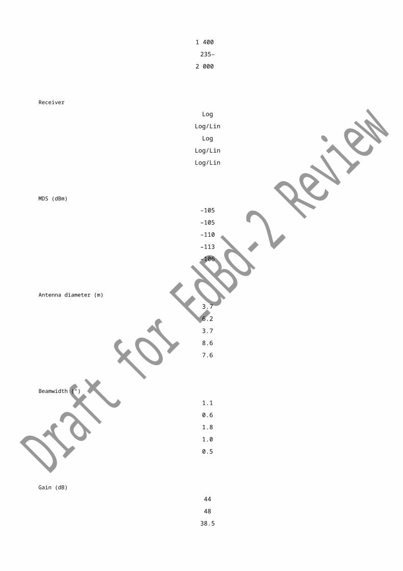
be done judiciously as tuning the adjustment for one situation may create problems in other situations. In situations where radar estimates are far from the mark due to radar calibration or other problems, such adjustments can bring about significant improvements.

Ground level precipitation estimates from radar systems are made for areas of typically 1-4 km 2 spatial resolution, successively for 5–15 minute periods using low elevation (elevation angles of <1o) plan position indicator (PPI) scans, constant altitude PPI (CAPPI) synthetic products or even more sophisticated products. The radar estimates have been found to compare with spot precipitation gauge measurements within a factor of two. The gauge samples an extremely small area (100 cm2, 200 cm2), while the radar integrates over a volume, on a much larger scale (1-4 k m2). This difference accounts for a considerable amount of the discrepancy. There are indications that the gauge ac-curacy may, for some purposes, be far inferior to what is commonly assumed, especially if the estimates come from a relatively small number of rain gauges (Neff, 1977). An important consideration is the success metric. Seasonal averages may be acceptable is some applications and a single Z-R relationship may be sufficient. However, for flash flood warnings, real-time adjustments may be required.

However, the adjustments do not automatically ensure improvements in radar estimates, and sometimes the ad -justed estimates are poorer than the original ones. This is especially true for convective rainfall where the vertical ex-tent of echo mitigates the difficulties associated with the vertical profile, and the gauge data are suspect because of unrepresentative sampling. Also, the spatial decorrelation distance may be small, and the gauge-radar comparison becomes increasingly inaccurate with distance from the gauge. A general guideline is that the adjustments will pro-duce consistent improvements only when the systematic differences (that is, the bias) between the gauge and radar rainfall estimates are larger than the standard deviation of the random scatter of the gauge versus radar compar -isons. This guideline makes it possible to judge whether gauge data should be used to make adjustments and leads to the idea that the available data should be tested before any adjustment is actually applied. Various methods for accomplishing this have been explored, but at this time there is no widely accepted approach.

Dual-Polarization Precipitation Techniques

Various techniques for using polarization diversity radar to improve rainfall measurements have been proposed. In particular, it has been suggested that the difference between reflectivities measured at horizontal and vertical polar-ization (ZDR) can provide useful information about drop-size distributions (Seliga and Bringi, 1976). An alternate method is to use KDP that depends on large oblate spheroids distorting the shape of the transmitted wave. The methods depends on the hydrodynamic distortions of the shapes of large raindrops, with more intense rainfalls with larger drops giving stronger polarization signatures – both in power and differential phase. There is still considerable research on whether this technique has promise for operational use for precipitation measurement (English and oth-ers, 1991). At long wavelengths, the rainrate threshold where Kdp techniques are effective are higher (for example, at S Band, it is about 20 mm/h and a X Band it is about 4 mm/h).

At close ranges (with high spatial resolution), polarization diversity radars may give valuable information about pre -cipitation particle distributions and other parameters pertinent to cloud physics. At longer ranges, it is impossible to be sure that the radar beam is filled with a homogeneous distribution of hydrometeors. Consequently, the empirical relationship of the polarimetric signature to the drop-size distribution increases uncertainty. Of course, knowing more about Z-R will help, but, even if multi-parameter techniques worked perfectly well, the error caused by Z-R could be reduced only from 33 to 17 per cent, as shown by Ulbrich and Atlas (1984). For short -range hydrological applica-tions, the corrections for other biases (already discussed) are usually much greater, perhaps by an order of magni -tude or more.

Wind Estimation/Wind Mapping

A Doppler radar measures only the radial (direction in which the radar is pointing) component of the wind. Retrieval of the missing tangential component requires spatial assumptions of the wind pattern. A single Doppler measure -ment at a single point can not be unambiguously interpreted.

On the large scale, if there is wide spread precipitation and it is assumed that the wind at a constant altitude is uni -form or linear over the radar domain, then a plot of the radial velocity with azimuth will show a sinusoid. The magni-tude and the azimuth of the largest radial velocity observed will indicate the speed and the direction of the wind. The plot and the technique is called the Velocity-Azimuth Display (VAD). With a radar scanning at constant elevation an-gle, the farther the range, the higher in altitude is the data. By applying the VAD technique to data at increasing range (increasing height), a wind profile can be derived. There are various variations on the technique where sparse data can be assumed. Note that non-precipitating or clear air echoes have great value in this application.

At smaller scales, the radial velocities are used to identify hazardous wind features of thunderstorms. Assumptions such as rotating, divergent or convergent flows, and various permutations and combinations, are assumed at scales of a few to tens of kilometers. These distinctive patterns have been used very successfully to identify mesocyclones, downbursts and gust fronts that produce hazardous winds. Tornadoes are generally too small to be observed di -rectly except very near the radar due to spatial resolution mis-matches.

Assimilation of radial velocities into small scale models are performed in research to retrieve the full wind field but the has not reached operational status.

Rain/snow/hail discrimination and other target classification

With conventional or reflectivity-only radars, the pattern and intensity of the echo was used to roughly estimate the nature of the target. In summer, reflectivities less than about 12 dBZ were considered to be non-precipitating echoes, light rain was up to about 30 dBZ and heavy rain up to about 50 dBZ or so. Reflectivities above 57 dBZ was considered to be hail. Snow is not generally separable with these kind of radars in the horizontal. In the vertical, the bright band (a region of enhanced reflectivity due to wet large snow aggregates) delineated snow aloft from rain below.

Airplanes were identified as isolated point anomalies and ground echoes were identified as stationary or permanent echoes at short range around the radar. The reflectivities of airplanes and ground echoes can vary greatly because small changes is aspect angle result in substantial changes in backscatter.

Doppler radars can identify non-moving targets such as ground clutter and anomalous propagation echoes even in the presence weather. These ground targets can be effectively filtered out in signal processing to produce “cor -rected (for ground clutter) reflectivity”. Most if not all modern radars have Doppler and have this capability. Before Doppler radars, a variety of techniques were used to remove ground clutter including: (i) use of CAPPI, (ii) use of ground clutter maps, (iii) use of the statistical fluctuation of the reflectivity statistics.

Dual-polarization radars characterize the target using reflectivity information from orthogonal channels, their cross-polar signal and changes in propagation phase. Surface temperature and humidity and soundings from numerical weather prediction models are also used. Fuzzy logic techniques use independent estimates from a variety dual-po -larization parameters to classify the echo type into a variety of categories including: ground clutter, rain, snow, hail, biological and even big and small drops.

Initiation and numerical weather prediction models

A variety of radar data and products are used for data assimilation in some numerical weather prediction centers. Not all models use the same products. Precipitation is a derived parameter in numerical weather prediction models and so it is difficult to directly assimilate precipitation or reflectivity fields. Wind are direct model variables and radial velocities may be assimilated with less contrivance. These include VAD wind profiles, composited radar derived surface precipitation fields in global models and in some cases, three dimensional reflectivity and radial velocity fields for local area or small scale models in polar coordinates . Lopez (20?) has demonstrated the value of assimi-lating the U.S. “Stage IV” surface precipitation product on the weather in Europe and Asia. These and other applica-tions (typhoon tracking) are prime drivers for the global weather radar data exchange initiative.

Humidity Estimation

An emerging innovation is the retrieval of humidity from beam propagation differences of echoes from the om-nipresent ground targets. This innovation is counter intuitive to the siting of weather radars since they are sited to minimize ground clutter. Index of refraction fluctuations cause beam propagation path length changes which can be detected as changes in the phase of the signal or the Doppler shift. By comparing the shift in dry versus moist con-ditions and accounting for range ambiguities, the path length change can be estimated and then related to the index of refraction change using Snell’s law. The index of refraction is dependent on temperature, pressure and humidity but primarily on the latter and hence the humidity can be retrieved very near the radar. Several research radars have this capability and some operational systems (in France and U.K.) are prototyping this for operational deploy-ment.

Radar Volume Scan Strategy

Most modern radars automatically perform a volume scan consisting of a number of full azimuth rotations of the an-tenna at several elevation angles. This is called the “scan strategy” and there are a variety of strategies for different purposes.

Long range scans of 500 km or more (that result in limited Nyquist velocity) are needed for long range surveillance. Rapid update of the order of 5 minutes is required to capture the evolving morphology of the convective thunder -storm. In aviation downburst applications, even shorter cycle times are required (TDWR ref). Research radars scan limited areas or sectors with one minute or less cycle times (Wurman ???). Slow low level scans with long pulse lengths are needed to maximize the capture of clear air echoes. Slow scanning will optimize the Doppler filtering of ground echoes. Multiple PRF techniques require the assumption of uniformity of radial velocity and can be imple -mented on a ray by ray or scan by scan basis.

Scans as low as possible are needed for precipitation estimates or to optimize the detection of low level weather. A geometric sequence of elevation angles are required to generate optimal Constant Altitude Plan Position Indicator or echo top products (Marshall and Ballantyne, 1978). The emerging and futuristic X Band phased array radar net -works such as that of the Co-operative Adaptive Sensing of the Atmosphere (CASA) project or the Multi-Purpose Ar-ray Radar (MPAR) revolutionize the scan strategy concept as the electronic scanning can adapt to the weather or

application (ref) or weaknesses may be mitigated with data from neighboring radars.

The trade-off is the quality of the data. For example, slow scans for high spectral resolution for ground clutter mitiga -tion or low data variance preclude scan strategies with very many elevation angles and hence result in poor vertical resolution. Data quality is a nebulous concept as it qualitatively refers to trade-offs in timeliness or temporal resolu -tion (cycle time), spatial resolution (azimuth, range, elevation), data bias (e.g. velocity or reflectivity bias) and data variance. This is difficult to objectively optimize as the success metrics are quite diverse and setting the number of elevation angle sequence is not an exact science.

Of prime consideration is the nature of the weather and the location that requires the coverage. For example, the scan sequence for a radar located in a valley used for local and short range application will or can be quite different from a radar that is used for long range surveillance for land falling hurricanes (Joe et al, 2013).

While it is attractive conceptually to set the elevation angles changes equal to the beam width, however due to the stratified nature of the precipitation (snow, bright band, rain profiles) and the wind profile, small changes in the eleva-tion angle of even of 0.1o degrees can produce significant views of the data (Fig. 9.x, Marshall and Ballantyne, 1978).

Raw polar data are stored in a three (range, azimuth, elevation) or multiple (radar parameter) dimensional array, commonly called the “volume scan”. This serves as the data source for further data processing and archiving. There can be several versions of raw data due to different data quality processing.

9.10 Meteorological products

The radar data can be processed to provide a variety of meteorological products to support various applications. The quality of the products that can be generated by a weather radar depend on the type of radar, its signal processing characteristics, and the associated radar control and data analysis/production system. By means of application soft -ware, a wide variety of meteorological products is generated and displayed as images on a high-resolution colour display monitor or sent as meta-products (e.g. a CAPPI product in raw reflectivity units) to a data visualization sys-tem.

These products include grids of raw or derived radar parameters, vertical wind profiles, location and characteristics of analyzed thunderstorm cells, their historical tracks and nowcasts etc. Grid or pixel values and conversion to x-y coordinates are computed using various two and three-dimensional interpolation techniques to grids with different geographical projections. For radar networks, the latter is an important considerations whereas with single radar im-agery, all the projections are very close.

For a typical Doppler weather radar, the displayed variables are reflectivity, radial velocity, radial velocity and spec-trum width, precipitation rate or accumulation. For dual-polarization radars, typical display variables are differential reflecitivity (Zdr), correlation (rhohv), differential phase (phidp), precipitation rate and particle classification.

The following is a list of common products generated:(a) The plan position indicator: A polar format display of a variable, obtained from a single full antenna rotation at

one selected elevation. It is the classic radar display, used primarily for weather surveillance; This is the most basic of products. Note that it is made at constant elevation angle and so increasing range means that the data is taken at increasing height. Any parameter is displayed in this format.

(b) The constant altitude plan position indicator (CAPPI): A horizontal cross-section display of a variable (usually reflectivity or rainrate) at a specified altitude, produced by interpolation from the volume data. It is used for sur -veillance and for identification of severe storms. It is also useful for monitoring the weather at specific flight lev -els for air traffic applications. One of the rationales for the CAPPI is that by judicious selection of the altitude, a near-clutter free product can be produced in the absence of the Doppler zero velocity notch filter.

(c) The pseudo range height indicator: A display of a variable obtained from a volume scan where the data from the same azimuth are extracted and collated to provide vertical information on the structure of the weather. Classically, this was done with a antenna doing a physical vertical sweep, typically from 0 to 90°, at one az-imuth. Manual intervention was required to select the azimuth and when to do the scan. The advantage of the classic technique is the density of information is much higher. Typically, very fine elevation angle changes (~ 0.1o) can be used. The quality of the pseudo RHI technique depends on the scan strategy but it has the great advantage of flexibility. It is used for identifying severe storms, hail and the bright band;

(d) Vertical cross-section: A display of a variable above a user-defined surface vector (not necessarily through the radar). It is produced by interpolation from the volume data; This is an interactive product and has largely re-placed the RHI product.

(e) The column maximum: A display, in plan, of the maximum value of a variable (usually reflectivity) above each point of the area being observed; This is useful to identify the maximum reflectivity in a storm to assess its severity or to estimate the maximum precipitation that could be expected to fall from a storm. In some cases, due to radar siting issues, where the low levels can not be observed (mountainous terrain), this was used to estimate surface precipitation. Sometimes, there is a minimum altitude threshold to the data, so that the high reflectivities in the bright band does not overly influence the use of this product.

(g) Vertically integrated liquid: An indicator of the intensity of severe storms. It can be displayed, in plan, for any specified layer of the atmosphere. As this is dominated by the highest reflectivities, this is very similar to the

maximum reflectivity product in pattern but in different units.

(f) Echo tops: A display, in plan, of the height of the highest occurrence of a selectable reflectivity contour, ob-tained by searching in the volume data. It is an indicator of the strength of the updraft and therefore a indicator of severe weather and hail;

(h) Often the reflectivity products are converted to precipitation products by an empirical relationship between Z and R. There are many relationships published but remarkably the original proposed relationship by Marshall and Palmer is still widely used. Dual polarization radar has extended and improved the estimation of precipita -tion particularly at high precipitation rates. These precipitation products are aggregated into accumulation products of varying time duration. ???

(h) Modern computing system have significant processing capabilities. Techniques or algorithms have been devel-oped to search the 3 dimensional data to locale and quantify the characteristics of contiguous areas of high re-flectivity which are related to severe weather thunderstorms for the analyst (Fig. 9.x).

Product Description ProductDescription

Precipitation Product Cell Identification

Accumulation Product Cell Tracking/Nowcast

Basin Product Severity

Cross-correlation/nowcast reflectivity or precipitation Mesocyclone

Target Classification Downburst

Precipitation Type Downdraft

Hail Probability Bounded Weak Echo Region

Hail Size Storm Classification Identification and Tracking

Mosaic Cross-section

Velocity Azimuth Display

In addition to these standard or basic displays, other products can be generated to meet the particular requirements of users for purposes such as hydrology, nowcasting (see section 9.10) or aviation:(a) Precipitation-accumulation: An estimate of the precipitation accumulated over time at each point in the area ob-

served;

(b) Precipitation sub-catchment totals: Area-integrated accumulated precipitation;(c) Velocity azimuth display (VAD): An estimate of the vertical profile of wind above the radar. It is computed from

a single antenna rotation at a fixed elevation angle; Velocity volume processing, which uses three-dimensional volume data;

(d) Storm tracking: A product from complex software to determine the tracks of storm cells and to predict future lo-cations of storm centroids;

(e) Wind shear: An estimate of the radial and tangential wind shear at a height specified by the user;(f) Divergence profile: An estimation of divergence from the radial velocity data from which divergence profile is

obtained given some assumptions;(g) Mesocyclone: A product from sophisticated pattern recognition software that identifies rotation signatures

within the three-dimensional base velocity data that are on the scale of the parent mesocyclonic circulation of-ten associated with tornadoes;Tornadic vortex signature: A product from sophisticated pattern recognition soft -ware that identifies gate-to-gate shear signatures within the three-dimensional base velocity data that are on the scale of tornadic vortex circulations.

For a dual-polarization radar, there are various PPI products of the basic parameters (ZDR, RPHOhv, …). However, particle classification is the primary product for the end user – the forecaster. This product leads to a hail identifica-tion and rain-snow precipitation type product. Other advantages of the radar, such as data quality, are encom -passed by improvements in the accuracy of the existing products.

In addition, network processing results in a radar mosaic. Consideration for radar products are (i) projections are used for visualization of the data. (ii) For areas of overlapping radar coverage, various algorithms are used – either nearest radar, maximum value or one based on a sophisticated estimation of data quality. In the situation where the overlap is significant, a neighboring radar may fill the void in the "cone of silence". Two dimensional winds may con -ceivably be retrieved using dual-doppler concepts however, the overlap areas are not generally extensive and the errors may not be acceptable since the radars are so far apart.

Clear air echoes are persistent echoes around the radar that are attributable to the presence of insects or fluctua-tions in the index of refraction (Bragg scattering). Studies have indicated that these echoes are predominantly due to insects. These echoes have great value for analysis of convective initiation and wind estimation in non-precipitat-ing conditions and hence for data assimilation but need to be filtered for quantitive precipitation estimation.

9.11 Summary

Weather radar is arguably the most complex weather instrument used for operational applications. Compared to other meteorological sensor, it is still a rapidly changing technology. The latest technology is dual-polarization and networks of X Band phased array and other larger phased array antenna technology. Pulse compression solid state radars are now being deployed in several countries. Scientific expertise and expert advice is needed to optimally procure and configure a radar and a radar network. Decisions regarding procurement or operation of a weather radar or a radar network should be predicated on the ability to support and maintain a radar.

The use of weather radar has been justified for qualitative applications such as weather surveillance, the issuance of weather warnings, nowcasting and scientific understanding. It has been used by a human analyst who can over-come the artifacts in the data. Significant advances in the use of the weather radar data include advanced nowcast -ing techniques that take advantage of the ability of the radar to see clear air echoes, to be assimilated in numerical weather prediction data assimilation and modeling systems and even in the retrieval of humidity fields from ground echoes.

There are many adjustments needed to the data to remove the physical artifacts, to reduce the uncertainty in the data for quantitative precipitation estimates and to remove the bias or calibrate the radar data. The breakthrough development and robustness of the Simultaneous Transmission And Receive dual-polarization technology has al-lowed for its operational deployment which addresses these issues.

REFERENCES AND FURTHER READING

Ahnert, P.R., M. Hudlow, E. Johnson, D. Greene and M. Dias, 1983: Proposed on-site processing system for NEXRAD. Preprints of the Twenty-first Conference on Radar Meteorology (Edmonton, Canada), American Mete-orological Society, Boston, pp. 378–385.

Aoyagi, J., 1983: A study on the MTI weather radar system for rejecting ground clutter. Papers in Meteorology and Geophysics, Volume 33,

Number 4, pp. 187–243.

Aoyagi, J. and N. Kodaira, 1995: The reflection mechanism of radar rain echoes. Preprints of the Twenty-seventh Conference on Radar Meteorology (Vail, Colorado), American Meteorological Society, Boston, pp. 246–248.

Atlas, D., 1964: Advances in radar meteorology. Advances in Geophysics (H.E. Landsberg and J. Van Meighem, eds.), Volume 10, Academic Press, New York, pp. 317–479.Atlas, D. (ed.), 1990: Radar in Meteorology. American Meteorological Society, Boston.Atlas, D., R.C. Scrivastava and R.S. Sekhon, 1973: Doppler radar characteristics of precipitation at vertical inci -

dence. Reviews of Geophysics and Space Physics, Volume 11, Number 1, pp. 1–35.Battan, L.J., 1981: Radar Observation of the Atmosphere. University of Chicago Press, Chicago.Baynton, H.W., 1979: The case for Doppler radars along our hurricane affected coasts. Bulletin of the American Me-

teorological Society, Volume 60, pp. 1014–1023.Bean, B.R. and E.J. Dutton, 1966: Radio Meteorology. Washington DC, U.S. Government Printing Office.Bebbington, D.H.O., 1992: Degree of Polarization as a Radar Parameter and its Susceptibility to Coherent Propaga -

tion Effects. Preprints from URSI Commission F Symposium on Wave Propagation and Remote Sensing (Ravenscar, United Kingdom) pp. 431–436.

Bringi, V.N. and A. Hendry, 1990: Technology of polarization diversity radars for meteorology. In: Radar in Meteorol-ogy (D. Atlas, ed.) American Meteorological Society, Boston, pp. 153–190.

Browning, K.A. and R. Wexler, 1968: The determination of kinetic properties of a wind field using Doppler radar. Journal of Applied Meteorology, Volume 7, pp. 105–113.

Brown, R.A. and L.R. Lemon, 1976: Single Doppler radar vortex recognition: Part II – Tornadic vortex signatures. Preprints of the Seventeenth Conference on Radar Meteorology (Seattle, Washington), American Meteorological Society, Boston, pp. 104–109.

Browning, K.A. and C.G. Collier, 1982: An integrated radar-satellite nowcasting system in the United Kingdom. In: Nowcasting (K.A. Browning, ed.). Academic Press, London, pp. 47–61.

Browning, K.A., C.G. Collier, P.R. Larke, P. Menmuir, G.A. Monk and R.G. Owens, 1982: On the forecasting of frontal rain using a weather radar network. Monthly Weather Review, Volume 110, pp. 534–552.

Burgess, D.W., 1976: Single Doppler radar vortex recognition: Part I – Mesocyclone signatures. Preprints of the Sev-enteenth Conference on Radar Meteorology, (Seattle, Washington), American Meteorological Society, Boston, pp. 97–103.

Burgess, D.W. and L.R. Lemon, 1990: Severe thunderstorm detection by radar. In Radar in Meteorology (D. Atlas, ed.). American Meteorological Society, Boston, pp. 619–647.

Burrows, C.R. and S.S. Attwood, 1949: Radio Wave Propagation. Academic Press, New York.Byers, H.R., 1948: The use of radar in determining the amount of rain falling over a small area. Transactions of the

American Geophysical Union, pp. 187–196.Cluckie, I.D. and M.E. Owens, 1987: Real-time Rainfall Run-off Models and Use of Weather Radar Information. In:

Weather Radar and Flood Forecasting (V.K. Collinge and C. Kirby, eds). John Wiley and Sons, New York.Collier, C.G., 1989: Applications of Weather Radar Systems: A Guide to Uses of Radar Data in Meteorology and Hy-

drology. John Wiley and Sons, Chichester, England.Commission of the European Communities, 1990: Une revue du programme ARAMIS (J.L. Cheze). Seminar on Cost Project 73: Weather Radar Networking (Brussels, 5–8 September 1989), pp. 80–85.Crozier, C.L., P. Joe, J. Scott, H. Herscovitch and T. Nichols, 1991: The King City operational Doppler radar: Development, all-season applications and forecasting. At-

mosphere-Ocean, Volume, 29, pp. 479–516.Dennis, A.S., C.A. Schock, and A. Koscielski, 1970: Characteristics of hailstorms of western South Dakota. Journal

of Applied Meteorology, Volume 9, pp. 127–135.Dexter, P.E., M.L. Heron and J.F. Ward, 1982: Remote sensing of the sea-air interface using HF radars. Australian

Meteorological Magazine, Volume 30, pp. 31–41.Donaldson, R.J., Jr., 1970: Vortex signature recognition by a Doppler radar. Journal of Applied Meteorology, Volume

9, pp. 661–670.Doneaud, A.A., S. Ionescu-Niscov, D.L. Priegnitz and P.L. Smith, 1984: The area-time integral as an indicator for

convective rain volumes. Journal of Climate and Applied Meteorology, Volume 23, pp. 555–561.Doneaud, A.A., J.R. Miller Jr., L.R. Johnson, T.H. Vonder Haar and P. Laybe, 1987: The area-time integral technique to estimate convective rain volumes over ar-

eas applied to satellite data: A preliminary investigation. Journal of Climate and Applied Meteorology, Volume 26,

pp. 156–169.Doviak, R.J. and D.S. Zrnic, 1993: Doppler Radar and Weather Observations. Second edition, Academic Press, San

Diego.Eccles, P.J. and D. Atlas, 1973: A dual-wavelength radar hail detector. Journal of Applied Meteorology, Volume 12,

pp. 847–854.Eilts, M.D. and S.D. Smith, 1990: Efficient dealiasing of Doppler velocities using local environment constraints. Jour-

nal of Atmospheric and Oceanic Techonology, Volume 7, pp. 118–128.English, M.E., B. Kochtubajda, F.D. Barlow, A.R. Holt and R. McGuiness, 1991: Radar measurement of rainfall by differential propagation phase: A pilot experi -

ment. Atmosphere-Ocean, Volume 29, pp. 357–380.Federer, B., A. Waldvogel, W. Schmid, F. Hampel, E. Rosini, D. Vento and P. Admirat, 1978: Grossversuch IV: Design of a randomized hail suppression experiment us-

ing the Soviet method. Pure and Applied Geophysics, 117, pp. 548–571.Gossard, E.E. and R.G. Strauch, 1983: Radar Observations of Clear Air and Clouds. Elsevier Scientific Publication,

Amsterdam.Harlan, J.A. and T.M. Georges, 1994: An empirical relation between ocean-surface wind direction and the Bragg line

ratio of HF radar sea echo spectra. Journal of Geophysical Research, Volume 99, C4, pp. 7971–7978.Heiss, W.H., D.L. McGrew, and D. Sirmans, 1990: NEXRAD: Next generation weather radar (WSR-88D). Microwave

Journal, Volume 33, Number 1, pp. 79–98.Holleman, I., 2001: Hail Detection Using Single-polarization Radar. Scientific Report, Royal Netherlands Meteorolog-

ical Institute (KNMI) WR-2001-01, De Bilt.Holleman, I., H.R.A. Wessels, J.R.A. Onvlee and S.J.M. Barlag, 2000: Development of a hail-detection product. Physics and Chemistry of the Earth, Part B, 25, pp.

1293–1297.Holt, A.R., M. Chandra, and S.J. Wood, 1995: Polarisation diversity radar observations of storms at C-Band. Pre-

prints of the Twenty-seventh Conference on Radar Meteorology (Vail, Colorado), American Meteorological Soci-ety, Boston,

pp. 188–189.Holt, A.R., P.I. Joe, R. McGuinness and E. Torlaschi, 1993: Some examples of the use of degree of polarization in

interpreting weather radar data. Proceedings of the Twenty-sixth International Conference on Radar Meteorol-ogy, American Meteorological Society, pp. 748–750.

Joe, P., R.E. Passarelli and A.D. Siggia, 1995: Second trip unfolding by phase diversity processing. Preprints of the Twenty-seventh Conference on Radar Meteorology (Vail, Colorado), American Meteorological Society, Boston, pp. 770–772.

Joint Doppler Operational Project, 1979: Final Report on the Joint Doppler Operational Project. NOAA Technical Memorandum, ERL NSSL-86, Norman, Oklahoma, National Severe Storms Laboratory.

Joss, J. and A. Waldvogel, 1990: Precipitation measurement and hydrology. In: Radar in Meteorology (D. Atlas, ed.), American Meteorological Society, Boston, pp. 577–606.

Joss, J. and R.W. Lee, 1993: Scan strategy, clutter suppression calibration and vertical profile corrections. Preprints of the Twenty-sixth Conference on Radar Meteorology (Norman, Oklahoma), American Meteorological Society, Boston, pp. 390–392.

Keeler, R.J., C.A. Hwang and E. Loew, 1995: Pulse compression weather radar waveforms. Preprints of the Twenty-seventh Conference on Radar Meteorology (Vail, Colorado), American Meteorological Society, Boston, pp. 767–769.

Keenan, T.D. and S.J. Anderson, 1987: Some examples of surface wind field analysis based on Jindalee skywave radar data. Australian Meteorological Magazine, 35, pp. 153–161.

Leber, G.W., C.J. Merrit, and J.P. Robertson, 1961: WSR-57 Analysis of Heavy Rains. Preprints of the Ninth Weather Radar Conference, American Meteorological Society, Boston, pp. 102–105.

Lee, R., G. Della Bruna and J. Joss, 1995: Intensity of ground clutter and of echoes of anomalous propagation and its elimination. Preprints of the Twenty-seventh Conference on Radar Meteorology (Vail, Colorado), American Meteorological Society, Boston, pp. 651–652.

Lemon, L.R., D.W. Burgess and R.A. Brown, 1978: Tornadic storm airflow and morphology derived from single-Doppler radar measurements. Monthly Weather Review, Volume 106,

pp. 48–61.Leone, D.A., R.M. Endlich, J. Petriceks, R.T.H. Collis and J.R. Porter, 1989: Meteorological considerations used in

planning the NEXRAD network. Bulletin of the American Meteorological Society, Volume, 70, pp. 4–13.Lhermitte, R. and D. Atlas, 1961: Precipitation motion by pulse Doppler radar. Preprints of the Ninth Weather Radar

Conference, American Meteorological Society, Boston, pp. 218–233.Makihara, Y., 2000: Algorithms for precipitation nowcasting focused on detailed analysis using radar and raingauge

data. Technical Report of the Meteorological Research Institute, JMA, 39, pp. 63–111.Marshall, J.S. and K.L.S. Gunn, 1952: Measurement of snow parameters by radar. Journal of Meteorology, Volume

9, pp. 322–327.Marshall, J.S. and W.M. Palmer, 1948: The distribution of raindrops with size. Journal of Meteorology, Volume 5, pp.

165–166.Melnikov, V., D.S. Zrnic, R.J. Dovink and J.K. Carter, 2002: Status of the dual polarization upgrade on the NOAA’s

research and development WSR-88D. Preprints of the Eighteenth International Conference on Interactive Infor-mation Processing Systems (Orlando, Florida), American Meteorological Society, Boston, pp. 124–126.

Michelson, M., W.W. Schrader and J.G. Wilson, 1990: Terminal Doppler weather radar. Microwave Journal, Volume 33, Number 2,

pp. 139–148.Mie, G., 1908: Beiträge zur Optik träber Medien, speziell kolloidaler Metalläsungen. Annalen der Physik, 25, pp.

377–445.Mueller, C.K. and R.E. Carbone, 1987: Dynamics of a thunderstorm outflow. Journal of the Atmospheric Sciences,

Volume 44, pp. 1879–1898.Mueller, E.A., S.A. Rutledge, V.N. Bringi, D. Brunkow, P.C. Kennedy, K. Pattison, R. Bowie and V. Chandrasekar, 1995: CSU-CHILL radar upgrades. Preprints of the Twenty-seventh Conference on Radar Meteo-

rology (Vail, Colorado), American Meteorological Society, Boston, pp. 703–706.Neff, E.L., 1977: How much rain does a rain gauge gage? Journal of Hydrology, Volume 35, pp. 213–220.Passarelli, R.E., Jr., P. Romanik, S.G. Geotis and A.D. Siggia, 1981: Ground clutter rejection in the frequency domain. Preprints of the Twentieth Conference on Radar

Meteorology (Boston, Massachusetts), American Meteorological Society, Boston, pp. 295–300.Probert-Jones, J.R., 1962: The radar equation in meteorology. Quarterly Journal of the Royal Meteorological Soci-

ety, Volume 88, pp. 485–495.Ray, P.S., C.L. Ziegler, W. Bumgarner and R.J. Serafin, 1980: Single- and multiple-Doppler radar observations of

tornadic storms. Monthly Weather Review, Volume 108, pp. 1607–1625.Rinehart, R.E., 1991: Radar for Meteorologists. Grand Forks, North Dakota, University of North Dakota, Department

of Atmopheric Sciences.Ruggiero, F.H. and R.J. Donaldson, Jr., 1987: Wind field derivatives: A new diagnostic tool for analysis of hurricanes

by a single Doppler radar. Preprints of the Seventeenth Conference on Hurricanes and Tropical Meteorology (Miami, Florida), American Meteorological Society, Boston, pp. 178–181.

Sauvageot, H., 1982: Radarmétéorologie. Eyrolles, Paris.Sauvageot, H., 1994: Rainfall measurement by radar: A review. Atmospheric Research, Volume 35, pp. 27–54.Seliga, T.A. and V.N. Bringi, 1976: Potential use of radar differential reflectivity measurements at orthogonal polar -

izations for measuring precipitation. Journal of Applied Meteorology, Volume 15, pp. 69–76.Shearman, E.D. R., 1983: Radio science and oceanography. Radio Science, Volume 18, Number 3, pp. 299–320.Skolnik, M.I. (ed.), 1970: Radar Handbook. McGraw-Hill, New York.Smith, P.L., 1990: Precipitation measurement and hydrology: Panel report. In: Radar in Meteorology. (D. Atlas, ed.),

American Meteorological Society, Boston, pp. 607–618.Smith, P.L., 1995: Dwell time considerations for weather radars. Preprints of the Twenty-seventh Conference on

Radar Meteorology (Vail, Colorado), American Meteorological Society, Boston, pp. 760–762.Strauch, R.G., 1981: Comparison of meteorological Doppler radars with magnetron and klystron transmitters. Pre-

prints of the Twentieth Conference on Radar Meteorology (Boston, Massachusetts), American Meteorological Society, Boston,

pp. 211–214.Ulbrich, C.W. and D. Atlas, 1984: Assessment of the contribution of differential polarization to improve rainfall mea-

surements. Radio Science, Volume 19, Number 1, pp. 49–57.Wilson, J.W. and W.E. Schreiber, 1986: Initiation of convective storms at radar-observed boundary-layer conver-

gence lines. Monthly Weather Review, Volume 114, pp. 2516–2536.Wood, V.T. and R.A. Brown, 1986: Single Doppler velocity signature interpretation of nondivergent environmental

winds. Journal of Atmospheric and Oceanic Technology, Volume 3, pp. 114–128.World Meteorological Organization, 1985: Use of Radar in Meteorology (G.A. Clift). Technical Note No. 181,

WMO-No. 625, Geneva.Wurman, J., M. Randall and C. Burghart, 1995: Real-time vector winds from a bistatic Doppler radar network. Pre-

prints of the Twenty-seventh Conference on Radar Meteorology (Vail, Colorado), American Meteorological Soci-ety, Boston,

pp. 725–728.Zrnic, D.S. and S. Hamidi, 1981: Considerations for the Design of Ground Clutter Cancelers for Weather Radar . Re-

port DOT/FAA/RD-81/72, NTIS, pp. 77.Zrnic, D.S. and A.V. Ryzhkov, 1995: Advantages of rain measurements using specific differential phase. Preprints of

the Twenty-seventh Conference on Radar Meteorology (Vail, Colorado), American Meteorological Society, pp. 35–37.