View-Dependent Simplification Of Arbitrary Polygonal Environments David Luebke, Carl Erikson

Department of Computer Science University of North Carolina at Chapel Hill

1. ABSTRACT Hierarchical dynamic simplification (HDS) is a new approach to the problem of simplifying arbitrary polygonal environments. HDS operates dynamically, retessellating the scene continuously as the user’s viewing position shifts, and adaptively, processing the entire database without first decomposing the environment into individual objects. The resulting system allows real-time display of very complex polygonal CAD models consisting of thousands of parts and hundreds of thousands of polygons. HDS supports various preprocessing algorithms and various run-time criteria, providing a general framework for dynamic view-dependent simplification.

Briefly, HDS works by clustering vertices together in a hierarchical fashion. The simplification process continuously queries this hierarchy to generate a scene containing only those polygons that are important from the current viewpoint. When the volume of space associated with a vertex cluster occupies less than a user-specified amount of the screen, all vertices within that cluster are collapsed together and degenerate polygons filtered out. HDS maintains an active list of visible polygons for rendering. Since frame-to-frame movements typically involve small changes in viewpoint, and therefore modify the active list by only a few polygons, the method takes advantage of temporal coherence for greater speed.

CR Categories: I.3.5 [Computer Graphics]: Computational Geometry and Object Modeling - surfaces and object representations.

Additional Keywords: polygonal simplification, level of detail, view dependent rendering.

2. INTRODUCTION

2.1 Polygons In Computer Graphics Polygonal models currently dominate the field of interactive three-dimensional computer graphics. This is largely because their mathematical simplicity allows rapid rendering of polygonal datasets, which in turn has led to widely available polygon-rendering hardware. Moreover, polygons serve as a sort of lowest common denominator for computer models, since almost any model representation (spline, implicit-surface, volumetric) can be converted with arbitrary accuracy to a polygonal mesh.

In many cases the complexity of such models exceeds the capability of graphics hardware to render them interactively. Three approaches are used to alleviate this problem:

• Augmenting the raw polygonal data to convey more visual detail per polygon. Gouraud shading and texture mapping fall into this category.

• Using information about the model to cull away large portions which are occluded from the current viewpoint. The visibility processing approach of Teller and Sequin is an excellent example [Teller 91].

• Polygonal simplification methods simplify the polygonal geometry of small or distant objects to reduce the rendering cost without a significant loss in the visual content of the scene. HDS is one such method.

2.2 Polygonal Simplification Polygonal simplification is at once a very current and a very old topic in computer graphics. As early as 1976, James Clark described the benefits of representing objects within a scene at several resolutions, and flight simulators have long used hand-crafted multi-resolution models of airplanes to guarantee a constant frame rate [Clark 76, Cosman 81]. Recent years have seen a flurry of research into generating such multi-resolution representations of objects automatically by simplifying the polygonal geometry of the object. This paper presents a new approach which simplifies the geometry of entire scenes dynamically, adjusting the simplification as the user moves around.

2.3 Motivation The algorithm presented in this paper was conceived for very complex hand-crafted CAD databases, a class of models for which existing simplification methods are often inadequate. Real-world CAD models are often topologically unsound (i.e., non-manifold), and may entail a great deal of clean-up effort before many simplification algorithms can be applied. Sometimes such models even come in “polygon-soup” formats which do not differentiate individual objects, but instead describe the entire scene as an unorganized list of polygons. No existing algorithm deals elegantly with such models.

Even when the model format delineates objects, simplifying complex CAD datasets with current schemes can involve many man-hours. To begin with, physically large objects must be subdivided. Consider a model of a ship, for example: the hull of the ship should be divided into several sections, or the end furthest from the user will be tessellated as finely as the nearby hull. In addition, physically small objects may need to be combined, especially for drastic simplification. The diesel engine of that ship might consist of ten thousand small parts; a roughly engine-shaped block makes a better approximation than ten thousand tetrahedra. Finally, each simplification must be inspected for visual fidelity to the original object, and an appropriate switching threshold selected. This can be the most time-consuming step in the simplification of a complicated model with thousands of parts, but few existing techniques address automating the process.1

These considerations led to a new approach with three primary goals. First, the algorithm should be very general, making as few assumptions as possible about the input model. The algorithm must therefore deal robustly with degenerate and non-manifold models. Second, the algorithm should be completely automatic, able to simplify even a polygon-soup 1 Notable exceptions include work by Cohen et al, and by Shirley and

Maciel [Cohen 96, Maciel 95].

model without human intervention. This implies that the algorithm must simplify the entire scene adaptively rather than relying on simplifying objects within the scene. Third, the algorithm should be dynamically adjustable, supplying the system with a fine-grained interactive “dial” for trading off performance and fidelity. This final requirement implies that the algorithm must operate at least partially at run time.

2.4 Hierarchical Dynamic Simplification Hierarchical dynamic simplification has some novel features. Rather than representing the scene as a collection of objects, each at several levels of detail, the entire model comprises a single large data structure. This is the vertex tree, a hierarchy of vertices which is queried dynamically to generate a simplified scene. The vertex tree contains information only about the vertices and triangles of the model; manifold topology is not required and need not be preserved. Each node in the vertex tree contains one or more vertices; HDS operates by collapsing all of the vertices within a node together to a single representative vertex. Triangles whose corners have been collapsed together become redundant and can be eliminated, decreasing the total polygon count. Likewise, a node may be expanded by splitting its representative vertex into the representative vertices of the node’s children. Triangles filtered out when the node was collapsed become visible again when the node is expanded, increasing the polygon count.

The entire system is dynamic; nodes to be collapsed or expanded are continuously chosen based on their projected size. The screenspace extent of each node is monitored: as the viewpoint shifts, certain nodes in the vertex tree will fall below the size threshold. These nodes will be folded into their parent nodes and the now-redundant triangles removed from the display list. Other nodes will increase in apparent size to the user and will be unfolded into their constituent child nodes, introducing new vertices and new triangles into the display list. The user selects the screenspace size threshold and may adjust it during the course of a viewing session for interactive control over the degree of simplification. Nodes will be folded and unfolded each frame, so efficient methods for finding, adding, and removing the affected triangles are crucial.

3. STRUCTURES AND METHODS

3.1 Active Triangle List The purpose of the active triangle list is to take advantage of temporal coherence. Frames in an interactive viewing session typically exhibit only incremental shifts in viewpoint, so the set of visible triangles remains largely constant. The active triangle list in its simplest form is just a sequence of those visible triangles. Expanding a node appends some triangles to the active triangle list; collapsing the node removes them. The active list is maintained in the current implementation as a doubly-linked list of triangle structures, each with the following basic structure:

struct Tri {

Node * corners[3]; Node * proxies[3]; Tri *prev, *next; };

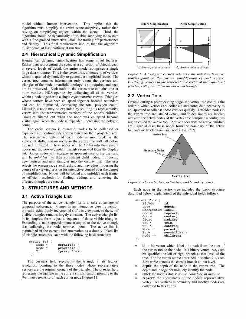
The corners field represents the triangle at its highest resolution, pointing to the three nodes whose representative vertices are the original corners of the triangle. The proxies field represents the triangle in the current simplification, pointing to the first active ancestor of each corner node [Figure 1].

Before Simplification After Simplification

(b) Arrows point at proxies(a) Arrows point at corners Figure 1: A triangle’s corners reference the initial vertices; its proxies point to the current simplification of each corner. Clustering vertices to the representative vertex of their quadrant (circled) collapses all but the darkened triangle.

3.2 Vertex Tree Created during a preprocessing stage, the vertex tree controls the order in which vertices are collapsed and stores data necessary to collapse and uncollapse these vertices quickly. Unfolded nodes in the vertex tree are labeled active, and folded nodes are labeled inactive; the active nodes of the vertex tree comprise a contiguous region called the active tree. Active nodes with no active children are a special case; these nodes form the boundary of the active tree and are labeled boundary nodes[Figure 2].

Boundary Nodes

Active Tree

Vertex Tree Figure 2: The vertex tree, active tree, and boundary nodes.

Each node in the vertex tree includes the basic structure described below (explanations of the individual fields follow):

struct Node { BitVec id; Byte depth; NodeStatus label; Coord repvert; Coord center; float radius; Tri * tris; Tri * subtris; Node * parent; Byte numchildren; Node ** children; }; • id: a bit vector which labels the path from the root of

the vertex tree to the node. In a binary vertex tree, each bit specifies the left or right branch at that level of the tree. For the vertex octree described in section 7.1, each 3-bit triple denotes the correct branch at that level.

• depth: the depth of the node in the vertex tree. The depth and id together uniquely identify the node.

• label: the node’s status: active, boundary, or inactive. • repvert: the coordinates of the node’s representative

vertex. All vertices in boundary and inactive nodes are collapsed to this vertex.

• center, radius: the center and radius of a bounding sphere containing all vertices in this node.

• tris: a list of triangles with exactly one corner in the node. These are the triangles whose corners must be adjusted when the node is folded or unfolded.

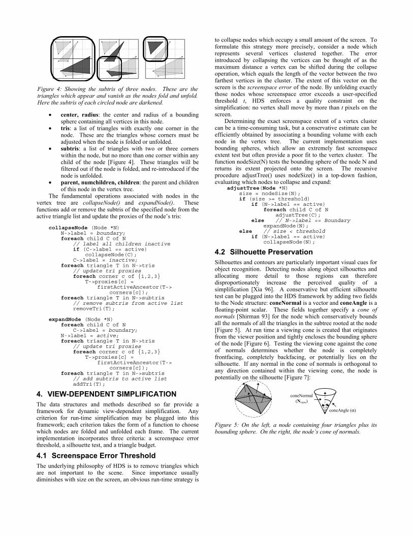
• subtris: a list of triangles with two or three corners within the node, but no more than one corner within any child of the node [Figure 4]. These triangles will be filtered out if the node is folded, and re-introduced if the node is unfolded.

• parent, numchildren, children: the parent and children of this node in the vertex tree.

The fundamental operations associated with nodes in the vertex tree are collapseNode() and expandNode(). These functions add or remove the subtris of the specified node from the active triangle list and update the proxies of the node’s tris:

collapseNode (Node *N) N->label = boundary; foreach child C of N

// label all children inactive if (C->label == active) collapseNode(C); C->label = inactive; foreach triangle T in N->tris

// update tri proxies foreach corner c of {1,2,3} T->proxies[c] = firstActiveAncestor(T-> corners[c]); foreach triangle T in N->subtris

// remove subtris from active list removeTri(T); expandNode (Node *N) foreach child C of N C->label = boundary; N->label = active; foreach triangle T in N->tris

// update tri proxies foreach corner c of {1,2,3} T->proxies[c] = firstActiveAncestor(T-> corners[c]); foreach triangle T in N->subtris

// add subtris to active list addTri(T);

4. VIEW-DEPENDENT SIMPLIFICATION The data structures and methods described so far provide a framework for dynamic view-dependent simplification. Any criterion for run-time simplification may be plugged into this framework; each criterion takes the form of a function to choose which nodes are folded and unfolded each frame. The current implementation incorporates three criteria: a screenspace error threshold, a silhouette test, and a triangle budget.

4.1 Screenspace Error Threshold The underlying philosophy of HDS is to remove triangles which are not important to the scene. Since importance usually diminishes with size on the screen, an obvious run-time strategy is

to collapse nodes which occupy a small amount of the screen. To formulate this strategy more precisely, consider a node which represents several vertices clustered together. The error introduced by collapsing the vertices can be thought of as the maximum distance a vertex can be shifted during the collapse operation, which equals the length of the vector between the two farthest vertices in the cluster. The extent of this vector on the screen is the screenspace error of the node. By unfolding exactly those nodes whose screenspace error exceeds a user-specified threshold t, HDS enforces a quality constraint on the simplification: no vertex shall move by more than t pixels on the screen.

Determining the exact screenspace extent of a vertex cluster can be a time-consuming task, but a conservative estimate can be efficiently obtained by associating a bounding volume with each node in the vertex tree. The current implementation uses bounding spheres, which allow an extremely fast screenspace extent test but often provide a poor fit to the vertex cluster. The function nodeSize(N) tests the bounding sphere of the node N and returns its extent projected onto the screen. The recursive procedure adjustTree() uses nodeSize() in a top-down fashion, evaluating which nodes to collapse and expand:

adjustTree(Node *N) size = nodeSize(N); if (size >= threshold) if (N->label == active) foreach child C of N adjustTree(C); else // N->label == Boundary expandNode(N); else // size < threshold if (N->label == active) collapseNode(N);

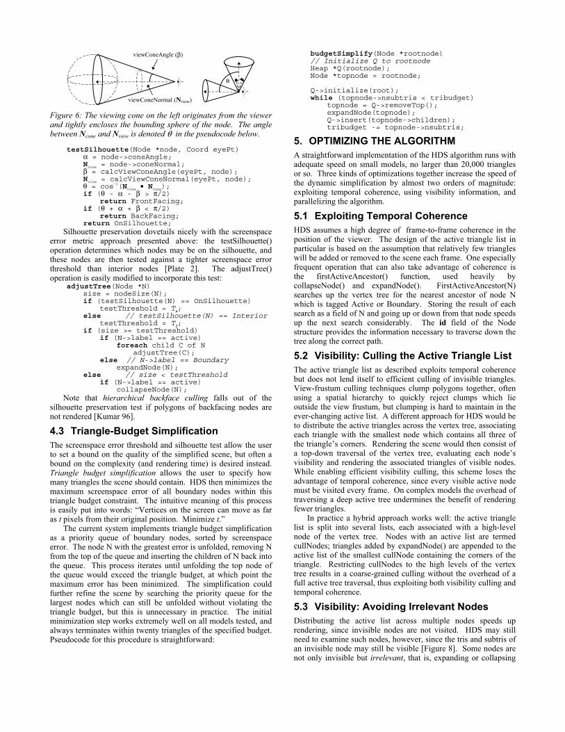
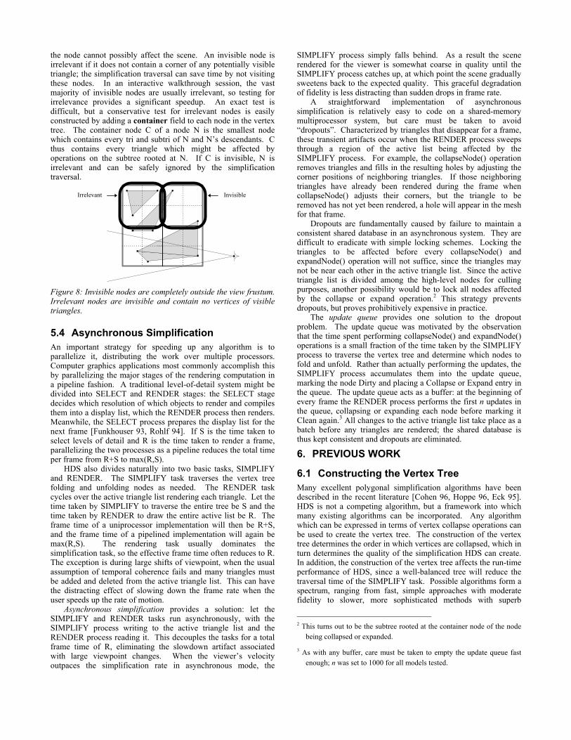
4.2 Silhouette Preservation Silhouettes and contours are particularly important visual cues for object recognition. Detecting nodes along object silhouettes and allocating more detail to those regions can therefore disproportionately increase the perceived quality of a simplification [Xia 96]. A conservative but efficient silhouette test can be plugged into the HDS framework by adding two fields to the Node structure: coneNormal is a vector and coneAngle is a floating-point scalar. These fields together specify a cone of normals [Shirman 93] for the node which conservatively bounds all the normals of all the triangles in the subtree rooted at the node [Figure 5]. At run time a viewing cone is created that originates from the viewer position and tightly encloses the bounding sphere of the node [Figure 6]. Testing the viewing cone against the cone of normals determines whether the node is completely frontfacing, completely backfacing, or potentially lies on the silhouette. If any normal in the cone of normals is orthogonal to any direction contained within the viewing cone, the node is potentially on the silhouette [Figure 7]:

coneNormal(Nview)

coneAngle (α)

Figure 5: On the left, a node containing four triangles plus its bounding sphere. On the right, the node’s cone of normals.

Figure 4: Showing the subtris of three nodes. These are the triangles which appear and vanish as the nodes fold and unfold. Here the subtris of each circled node are darkened.

viewConeNormal (Nview)

viewConeAngle (β)

θ

Figure 6: The viewing cone on the left originates from the viewer and tightly encloses the bounding sphere of the node. The angle between Ncone and Nview is denoted θ in the pseudocode below.

testSilhouette(Node *node, Coord eyePt) α = node->coneAngle; Ncone = node->coneNormal;

β = calcViewConeAngle(eyePt, node); Nview = calcViewConeNormal(eyePt, node); θ = cos-1(Nview • Ncone);

if (θ - α - β > π/2) return FrontFacing; if (θ + α + β < π/2) return BackFacing; return OnSilhouette;

Silhouette preservation dovetails nicely with the screenspace error metric approach presented above: the testSilhouette() operation determines which nodes may be on the silhouette, and these nodes are then tested against a tighter screenspace error threshold than interior nodes [Plate 2]. The adjustTree() operation is easily modified to incorporate this test:

adjustTree(Node *N) size = nodeSize(N); if (testSilhouette(N) == OnSilhouette) testThreshold = Ts; else // testSilhouette(N) == Interior testThreshold = TI; if (size >= testThreshold) if (N->label == active) foreach child C of N adjustTree(C); else // N->label == Boundary expandNode(N); else // size < testThreshold if (N->label == active) collapseNode(N);

Note that hierarchical backface culling falls out of the silhouette preservation test if polygons of backfacing nodes are not rendered [Kumar 96].

4.3 Triangle-Budget Simplification The screenspace error threshold and silhouette test allow the user to set a bound on the quality of the simplified scene, but often a bound on the complexity (and rendering time) is desired instead. Triangle budget simplification allows the user to specify how many triangles the scene should contain. HDS then minimizes the maximum screenspace error of all boundary nodes within this triangle budget constraint. The intuitive meaning of this process is easily put into words: “Vertices on the screen can move as far as t pixels from their original position. Minimize t.”

The current system implements triangle budget simplification as a priority queue of boundary nodes, sorted by screenspace error. The node N with the greatest error is unfolded, removing N from the top of the queue and inserting the children of N back into the queue. This process iterates until unfolding the top node of the queue would exceed the triangle budget, at which point the maximum error has been minimized. The simplification could further refine the scene by searching the priority queue for the largest nodes which can still be unfolded without violating the triangle budget, but this is unnecessary in practice. The initial minimization step works extremely well on all models tested, and always terminates within twenty triangles of the specified budget. Pseudocode for this procedure is straightforward:

budgetSimplify(Node *rootnode) // Initialize Q to rootnode Heap *Q(rootnode); Node *topnode = rootnode; Q->initialize(root); while (topnode->nsubtris < tribudget) topnode = Q->removeTop(); expandNode(topnode); Q->insert(topnode->children); tribudget -= topnode->nsubtris;

5. OPTIMIZING THE ALGORITHM A straightforward implementation of the HDS algorithm runs with adequate speed on small models, no larger than 20,000 triangles or so. Three kinds of optimizations together increase the speed of the dynamic simplification by almost two orders of magnitude: exploiting temporal coherence, using visibility information, and parallelizing the algorithm.

5.1 Exploiting Temporal Coherence HDS assumes a high degree of frame-to-frame coherence in the position of the viewer. The design of the active triangle list in particular is based on the assumption that relatively few triangles will be added or removed to the scene each frame. One especially frequent operation that can also take advantage of coherence is the firstActiveAncestor() function, used heavily by collapseNode() and expandNode(). FirstActiveAncestor(N) searches up the vertex tree for the nearest ancestor of node N which is tagged Active or Boundary. Storing the result of each search as a field of N and going up or down from that node speeds up the next search considerably. The id field of the Node structure provides the information necessary to traverse down the tree along the correct path.

5.2 Visibility: Culling the Active Triangle List The active triangle list as described exploits temporal coherence but does not lend itself to efficient culling of invisible triangles. View-frustum culling techniques clump polygons together, often using a spatial hierarchy to quickly reject clumps which lie outside the view frustum, but clumping is hard to maintain in the ever-changing active list. A different approach for HDS would be to distribute the active triangles across the vertex tree, associating each triangle with the smallest node which contains all three of the triangle’s corners. Rendering the scene would then consist of a top-down traversal of the vertex tree, evaluating each node’s visibility and rendering the associated triangles of visible nodes. While enabling efficient visibility culling, this scheme loses the advantage of temporal coherence, since every visible active node must be visited every frame. On complex models the overhead of traversing a deep active tree undermines the benefit of rendering fewer triangles.

In practice a hybrid approach works well: the active triangle list is split into several lists, each associated with a high-level node of the vertex tree. Nodes with an active list are termed cullNodes; triangles added by expandNode() are appended to the active list of the smallest cullNode containing the corners of the triangle. Restricting cullNodes to the high levels of the vertex tree results in a coarse-grained culling without the overhead of a full active tree traversal, thus exploiting both visibility culling and temporal coherence.

5.3 Visibility: Avoiding Irrelevant Nodes Distributing the active list across multiple nodes speeds up rendering, since invisible nodes are not visited. HDS may still need to examine such nodes, however, since the tris and subtris of an invisible node may still be visible [Figure 8]. Some nodes are not only invisible but irrelevant, that is, expanding or collapsing

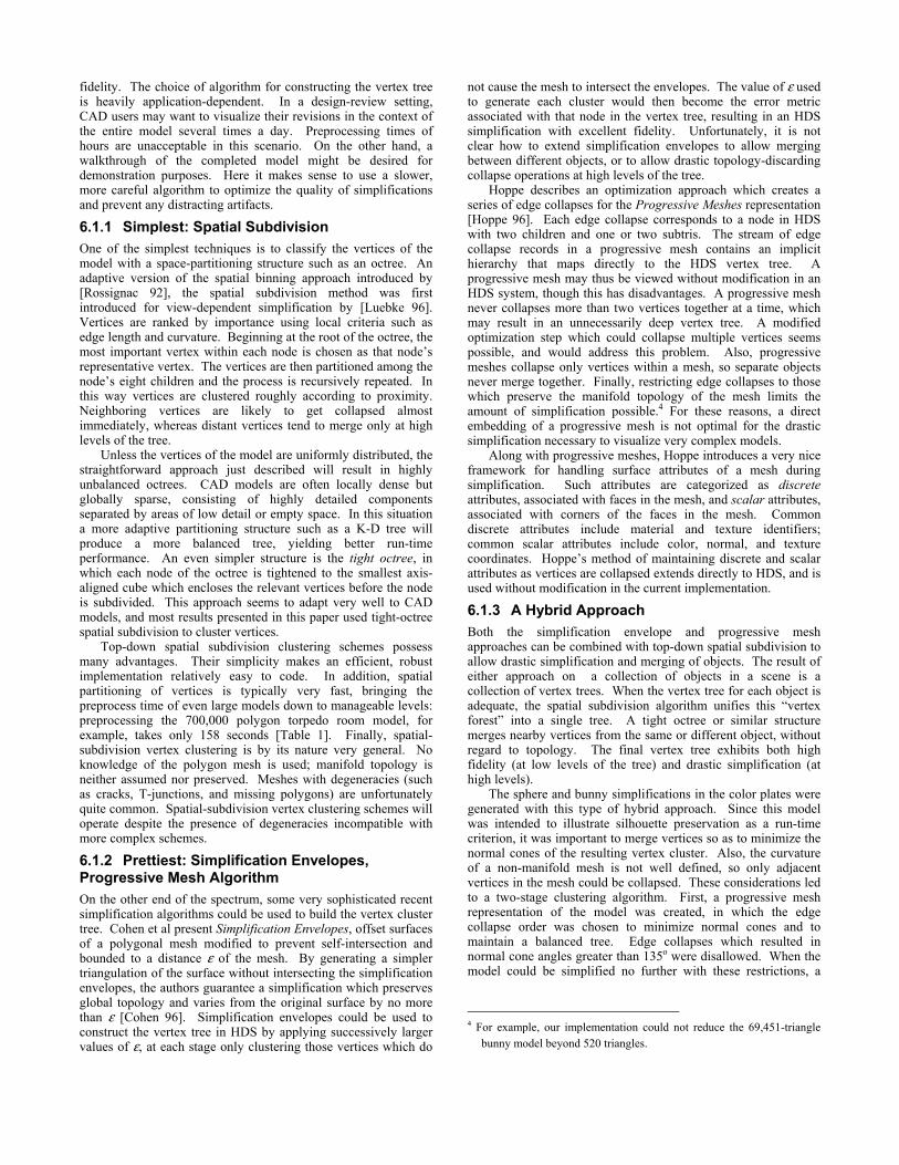
the node cannot possibly affect the scene. An invisible node is irrelevant if it does not contain a corner of any potentially visible triangle; the simplification traversal can save time by not visiting these nodes. In an interactive walkthrough session, the vast majority of invisible nodes are usually irrelevant, so testing for irrelevance provides a significant speedup. An exact test is difficult, but a conservative test for irrelevant nodes is easily constructed by adding a container field to each node in the vertex tree. The container node C of a node N is the smallest node which contains every tri and subtri of N and N’s descendants. C thus contains every triangle which might be affected by operations on the subtree rooted at N. If C is invisible, N is irrelevant and can be safely ignored by the simplification traversal.

Irrelevant Invisible

Figure 8: Invisible nodes are completely outside the view frustum. Irrelevant nodes are invisible and contain no vertices of visible triangles.

5.4 Asynchronous Simplification An important strategy for speeding up any algorithm is to parallelize it, distributing the work over multiple processors. Computer graphics applications most commonly accomplish this by parallelizing the major stages of the rendering computation in a pipeline fashion. A traditional level-of-detail system might be divided into SELECT and RENDER stages: the SELECT stage decides which resolution of which objects to render and compiles them into a display list, which the RENDER process then renders. Meanwhile, the SELECT process prepares the display list for the next frame [Funkhouser 93, Rohlf 94]. If S is the time taken to select levels of detail and R is the time taken to render a frame, parallelizing the two processes as a pipeline reduces the total time per frame from R+S to max(R,S).

HDS also divides naturally into two basic tasks, SIMPLIFY and RENDER. The SIMPLIFY task traverses the vertex tree folding and unfolding nodes as needed. The RENDER task cycles over the active triangle list rendering each triangle. Let the time taken by SIMPLIFY to traverse the entire tree be S and the time taken by RENDER to draw the entire active list be R. The frame time of a uniprocessor implementation will then be R+S, and the frame time of a pipelined implementation will again be max(R,S). The rendering task usually dominates the simplification task, so the effective frame time often reduces to R. The exception is during large shifts of viewpoint, when the usual assumption of temporal coherence fails and many triangles must be added and deleted from the active triangle list. This can have the distracting effect of slowing down the frame rate when the user speeds up the rate of motion.

Asynchronous simplification provides a solution: let the SIMPLIFY and RENDER tasks run asynchronously, with the SIMPLIFY process writing to the active triangle list and the RENDER process reading it. This decouples the tasks for a total frame time of R, eliminating the slowdown artifact associated with large viewpoint changes. When the viewer’s velocity outpaces the simplification rate in asynchronous mode, the

SIMPLIFY process simply falls behind. As a result the scene rendered for the viewer is somewhat coarse in quality until the SIMPLIFY process catches up, at which point the scene gradually sweetens back to the expected quality. This graceful degradation of fidelity is less distracting than sudden drops in frame rate.

A straightforward implementation of asynchronous simplification is relatively easy to code on a shared-memory multiprocessor system, but care must be taken to avoid “dropouts”. Characterized by triangles that disappear for a frame, these transient artifacts occur when the RENDER process sweeps through a region of the active list being affected by the SIMPLIFY process. For example, the collapseNode() operation removes triangles and fills in the resulting holes by adjusting the corner positions of neighboring triangles. If those neighboring triangles have already been rendered during the frame when collapseNode() adjusts their corners, but the triangle to be removed has not yet been rendered, a hole will appear in the mesh for that frame.

Dropouts are fundamentally caused by failure to maintain a consistent shared database in an asynchronous system. They are difficult to eradicate with simple locking schemes. Locking the triangles to be affected before every collapseNode() and expandNode() operation will not suffice, since the triangles may not be near each other in the active triangle list. Since the active triangle list is divided among the high-level nodes for culling purposes, another possibility would be to lock all nodes affected by the collapse or expand operation.2 This strategy prevents dropouts, but proves prohibitively expensive in practice.

The update queue provides one solution to the dropout problem. The update queue was motivated by the observation that the time spent performing collapseNode() and expandNode() operations is a small fraction of the time taken by the SIMPLIFY process to traverse the vertex tree and determine which nodes to fold and unfold. Rather than actually performing the updates, the SIMPLIFY process accumulates them into the update queue, marking the node Dirty and placing a Collapse or Expand entry in the queue. The update queue acts as a buffer: at the beginning of every frame the RENDER process performs the first n updates in the queue, collapsing or expanding each node before marking it Clean again.3 All changes to the active triangle list take place as a batch before any triangles are rendered; the shared database is thus kept consistent and dropouts are eliminated.

6. PREVIOUS WORK

6.1 Constructing the Vertex Tree Many excellent polygonal simplification algorithms have been described in the recent literature [Cohen 96, Hoppe 96, Eck 95]. HDS is not a competing algorithm, but a framework into which many existing algorithms can be incorporated. Any algorithm which can be expressed in terms of vertex collapse operations can be used to create the vertex tree. The construction of the vertex tree determines the order in which vertices are collapsed, which in turn determines the quality of the simplification HDS can create. In addition, the construction of the vertex tree affects the run-time performance of HDS, since a well-balanced tree will reduce the traversal time of the SIMPLIFY task. Possible algorithms form a spectrum, ranging from fast, simple approaches with moderate fidelity to slower, more sophisticated methods with superb

2 This turns out to be the subtree rooted at the container node of the node

being collapsed or expanded.

3 As with any buffer, care must be taken to empty the update queue fast enough; n was set to 1000 for all models tested.

fidelity. The choice of algorithm for constructing the vertex tree is heavily application-dependent. In a design-review setting, CAD users may want to visualize their revisions in the context of the entire model several times a day. Preprocessing times of hours are unacceptable in this scenario. On the other hand, a walkthrough of the completed model might be desired for demonstration purposes. Here it makes sense to use a slower, more careful algorithm to optimize the quality of simplifications and prevent any distracting artifacts.

6.1.1 Simplest: Spatial Subdivision One of the simplest techniques is to classify the vertices of the model with a space-partitioning structure such as an octree. An adaptive version of the spatial binning approach introduced by [Rossignac 92], the spatial subdivision method was first introduced for view-dependent simplification by [Luebke 96]. Vertices are ranked by importance using local criteria such as edge length and curvature. Beginning at the root of the octree, the most important vertex within each node is chosen as that node’s representative vertex. The vertices are then partitioned among the node’s eight children and the process is recursively repeated. In this way vertices are clustered roughly according to proximity. Neighboring vertices are likely to get collapsed almost immediately, whereas distant vertices tend to merge only at high levels of the tree.

Unless the vertices of the model are uniformly distributed, the straightforward approach just described will result in highly unbalanced octrees. CAD models are often locally dense but globally sparse, consisting of highly detailed components separated by areas of low detail or empty space. In this situation a more adaptive partitioning structure such as a K-D tree will produce a more balanced tree, yielding better run-time performance. An even simpler structure is the tight octree, in which each node of the octree is tightened to the smallest axis-aligned cube which encloses the relevant vertices before the node is subdivided. This approach seems to adapt very well to CAD models, and most results presented in this paper used tight-octree spatial subdivision to cluster vertices.

Top-down spatial subdivision clustering schemes possess many advantages. Their simplicity makes an efficient, robust implementation relatively easy to code. In addition, spatial partitioning of vertices is typically very fast, bringing the preprocess time of even large models down to manageable levels: preprocessing the 700,000 polygon torpedo room model, for example, takes only 158 seconds [Table 1]. Finally, spatial-subdivision vertex clustering is by its nature very general. No knowledge of the polygon mesh is used; manifold topology is neither assumed nor preserved. Meshes with degeneracies (such as cracks, T-junctions, and missing polygons) are unfortunately quite common. Spatial-subdivision vertex clustering schemes will operate despite the presence of degeneracies incompatible with more complex schemes.

6.1.2 Prettiest: Simplification Envelopes, Progressive Mesh Algorithm On the other end of the spectrum, some very sophisticated recent simplification algorithms could be used to build the vertex cluster tree. Cohen et al present Simplification Envelopes, offset surfaces of a polygonal mesh modified to prevent self-intersection and bounded to a distance ε of the mesh. By generating a simpler triangulation of the surface without intersecting the simplification envelopes, the authors guarantee a simplification which preserves global topology and varies from the original surface by no more than ε [Cohen 96]. Simplification envelopes could be used to construct the vertex tree in HDS by applying successively larger values of ε, at each stage only clustering those vertices which do

not cause the mesh to intersect the envelopes. The value of ε used to generate each cluster would then become the error metric associated with that node in the vertex tree, resulting in an HDS simplification with excellent fidelity. Unfortunately, it is not clear how to extend simplification envelopes to allow merging between different objects, or to allow drastic topology-discarding collapse operations at high levels of the tree.

Hoppe describes an optimization approach which creates a series of edge collapses for the Progressive Meshes representation [Hoppe 96]. Each edge collapse corresponds to a node in HDS with two children and one or two subtris. The stream of edge collapse records in a progressive mesh contains an implicit hierarchy that maps directly to the HDS vertex tree. A progressive mesh may thus be viewed without modification in an HDS system, though this has disadvantages. A progressive mesh never collapses more than two vertices together at a time, which may result in an unnecessarily deep vertex tree. A modified optimization step which could collapse multiple vertices seems possible, and would address this problem. Also, progressive meshes collapse only vertices within a mesh, so separate objects never merge together. Finally, restricting edge collapses to those which preserve the manifold topology of the mesh limits the amount of simplification possible.4 For these reasons, a direct embedding of a progressive mesh is not optimal for the drastic simplification necessary to visualize very complex models.

Along with progressive meshes, Hoppe introduces a very nice framework for handling surface attributes of a mesh during simplification. Such attributes are categorized as discrete attributes, associated with faces in the mesh, and scalar attributes, associated with corners of the faces in the mesh. Common discrete attributes include material and texture identifiers; common scalar attributes include color, normal, and texture coordinates. Hoppe’s method of maintaining discrete and scalar attributes as vertices are collapsed extends directly to HDS, and is used without modification in the current implementation.

6.1.3 A Hybrid Approach Both the simplification envelope and progressive mesh approaches can be combined with top-down spatial subdivision to allow drastic simplification and merging of objects. The result of either approach on a collection of objects in a scene is a collection of vertex trees. When the vertex tree for each object is adequate, the spatial subdivision algorithm unifies this “vertex forest” into a single tree. A tight octree or similar structure merges nearby vertices from the same or different object, without regard to topology. The final vertex tree exhibits both high fidelity (at low levels of the tree) and drastic simplification (at high levels).

The sphere and bunny simplifications in the color plates were generated with this type of hybrid approach. Since this model was intended to illustrate silhouette preservation as a run-time criterion, it was important to merge vertices so as to minimize the normal cones of the resulting vertex cluster. Also, the curvature of a non-manifold mesh is not well defined, so only adjacent vertices in the mesh could be collapsed. These considerations led to a two-stage clustering algorithm. First, a progressive mesh representation of the model was created, in which the edge collapse order was chosen to minimize normal cones and to maintain a balanced tree. Edge collapses which resulted in normal cone angles greater than 135o were disallowed. When the model could be simplified no further with these restrictions, a

4 For example, our implementation could not reduce the 69,451-triangle

bunny model beyond 520 triangles.

tight octree was applied to the remaining vertex clusters to produce a single HDS vertex tree.

6.2 Other Related Work Xia and Varshney use merge trees to perform view-dependent simplifications of triangular models in real-time [Xia 96]. A merge tree is similar to a progressive mesh, created off-line and consisting of a hierarchy of edge collapses. Selective refinement is applied based on viewing direction, lighting, and visibility. Xia and Varshney update an active list of vertices and triangles, using frame-to-frame coherence to achieve real-time performance. In addition, extra information is stored at each node of the merge tree to specify dependencies between edge collapse operations. These dependencies are used to eliminate folding artifacts during the visualization of the model, but also constrain the tessellation to change gradually between areas of high simplification and areas of low simplification. This restriction limits the degree of drastic simplification possible with a merge tree, as does the inability of merge trees to combine vertices from different objects. Xia and Varshney also assume manifold models, which together with the limited simplification available makes their approach less appropriate for large-scale CAD databases.

The error bounds described in Section 4 provide a useful indicator of the simplification fidelity, but screenspace error and silhouette preservation are only two of the many criteria that determine the view-dependent perceptual importance of a region of a scene. Ohshima et al. [Ohshima 96] investigate a gaze-directed system which allocates geometric detail to objects according to their calculated visual acuity. Objects in the center of vision have a higher visual acuity than objects in the periphery and are thus drawn at a higher level of detail. Similarly, stationary objects are assigned a higher visual acuity than rapidly moving objects, and objects at the depth of the user’s binocular fusion are assigned a higher visual acuity than objects closer or farther than the distance at which the user’s eyes currently converge. These techniques show promise for further reducing the polygon count of a scene in immersive rendering situations, and could be integrated into the HDS framework as additional run-time simplification criteria.

7. RESULTS HDS has been implemented and tested on a Silicon Graphics Onyx system with InfiniteReality graphics.

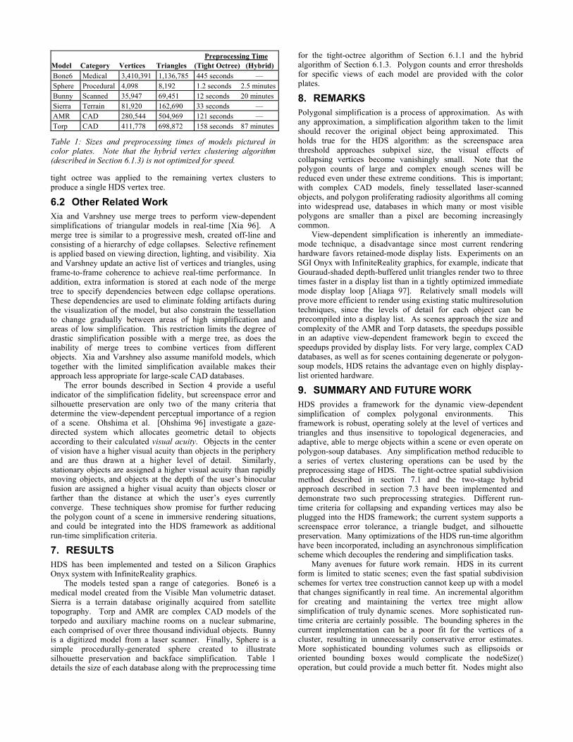
The models tested span a range of categories. Bone6 is a medical model created from the Visible Man volumetric dataset. Sierra is a terrain database originally acquired from satellite topography. Torp and AMR are complex CAD models of the torpedo and auxiliary machine rooms on a nuclear submarine, each comprised of over three thousand individual objects. Bunny is a digitized model from a laser scanner. Finally, Sphere is a simple procedurally-generated sphere created to illustrate silhouette preservation and backface simplification. Table 1 details the size of each database along with the preprocessing time

for the tight-octree algorithm of Section 6.1.1 and the hybrid algorithm of Section 6.1.3. Polygon counts and error thresholds for specific views of each model are provided with the color plates.

8. REMARKS Polygonal simplification is a process of approximation. As with any approximation, a simplification algorithm taken to the limit should recover the original object being approximated. This holds true for the HDS algorithm: as the screenspace area threshold approaches subpixel size, the visual effects of collapsing vertices become vanishingly small. Note that the polygon counts of large and complex enough scenes will be reduced even under these extreme conditions. This is important; with complex CAD models, finely tessellated laser-scanned objects, and polygon proliferating radiosity algorithms all coming into widespread use, databases in which many or most visible polygons are smaller than a pixel are becoming increasingly common.

View-dependent simplification is inherently an immediate-mode technique, a disadvantage since most current rendering hardware favors retained-mode display lists. Experiments on an SGI Onyx with InfiniteReality graphics, for example, indicate that Gouraud-shaded depth-buffered unlit triangles render two to three times faster in a display list than in a tightly optimized immediate mode display loop [Aliaga 97]. Relatively small models will prove more efficient to render using existing static multiresolution techniques, since the levels of detail for each object can be precompiled into a display list. As scenes approach the size and complexity of the AMR and Torp datasets, the speedups possible in an adaptive view-dependent framework begin to exceed the speedups provided by display lists. For very large, complex CAD databases, as well as for scenes containing degenerate or polygon-soup models, HDS retains the advantage even on highly display-list oriented hardware.

9. SUMMARY AND FUTURE WORK HDS provides a framework for the dynamic view-dependent simplification of complex polygonal environments. This framework is robust, operating solely at the level of vertices and triangles and thus insensitive to topological degeneracies, and adaptive, able to merge objects within a scene or even operate on polygon-soup databases. Any simplification method reducible to a series of vertex clustering operations can be used by the preprocessing stage of HDS. The tight-octree spatial subdivision method described in section 7.1 and the two-stage hybrid approach described in section 7.3 have been implemented and demonstrate two such preprocessing strategies. Different run-time criteria for collapsing and expanding vertices may also be plugged into the HDS framework; the current system supports a screenspace error tolerance, a triangle budget, and silhouette preservation. Many optimizations of the HDS run-time algorithm have been incorporated, including an asynchronous simplification scheme which decouples the rendering and simplification tasks.

Many avenues for future work remain. HDS in its current form is limited to static scenes; even the fast spatial subdivision schemes for vertex tree construction cannot keep up with a model that changes significantly in real time. An incremental algorithm for creating and maintaining the vertex tree might allow simplification of truly dynamic scenes. More sophisticated run-time criteria are certainly possible. The bounding spheres in the current implementation can be a poor fit for the vertices of a cluster, resulting in unnecessarily conservative error estimates. More sophisticated bounding volumes such as ellipsoids or oriented bounding boxes would complicate the nodeSize() operation, but could provide a much better fit. Nodes might also

Model

Category

Vertices

Triangles

Preprocessing Time (Tight Octree) (Hybrid)

Bone6 Medical 3,410,391 1,136,785 445 seconds — Sphere Procedural 4,098 8,192 1.2 seconds 2.5 minutes Bunny Scanned 35,947 69,451 12 seconds 20 minutes Sierra Terrain 81,920 162,690 33 seconds — AMR CAD 280,544 504,969 121 seconds — Torp CAD 411,778 698,872 158 seconds 87 minutes

Table 1: Sizes and preprocessing times of models pictured in color plates. Note that the hybrid vertex clustering algorithm (described in Section 6.1.3) is not optimized for speed.

be unfolded to devote more detail to regions containing specular highlights in the manner of [Cho 96] and [Xia 96], or to perceptually important regions using the gaze-directed heuristics described in [Oshima 96].

10. ACKNOWLEDGMENTS Special thanks to Fred Brooks, Greg Turk, and Dinesh Manocha for their invaluable guidance and support throughout this project. Funding for this work was provided by DARPA Contract DABT63-93-C-0048, and Lockheed Missile and Space Co., Inc. Additional funding was provided by National Center for Research Resources Grant NIH/NCCR P4RR02170-13. David Luebke is supported by an IBM Cooperative Fellowship; Carl Erikson is supported by an NSF Graduate Fellowship.

11. REFERENCES [Aliaga 97] Aliaga, Daniel. “SGI Performance Tips” (Talk). For more information see: http://www.cs.unc.edu/~aliaga/IR-perf.html.

[Cho 96] Cho, Y., U. Neumann, J. Woo. “Improved Specular Highlights with Adaptive Shading”, Computer Graphics International 96, June, 1996.

[Clark 76] Clark, James H. “Hierarchical Geometric Models for Visible Surface Algorithms,” Communications of the ACM, Vol 19, No 10, pp 547-554.

[Cohen 96] Cohen, J., A. Varshney, D. Manocha, G. Turk, H. Weber, P. Agarwal, F. Brooks, W. Wright. “Simplification Envelopes”, Computer Graphics, Vol 30 (SIGGRAPH 96).

[Cosman 81] Cosman, M., and R. Schumacker. “System Strategies to Optimize CIG Image Content”. Proceedings Image II Conference (Scotsdale, Arizona), 1981.

[Eck 95] Eck, M., T. DeRose, T. Duchamp, H. Hoppe, M. Lounsbery, W. Stuetzle. “Multiresolution Analysis of Arbitrary Meshes”, Computer Graphics, Vol 29 (SIGGRAPH 95).

[Funkhouser 93] Funkhouser, Thomas, and Carlo Sequin. “Adaptive Display Algorithm for Interactive Frame Rates During Visualization of Complex Virtual Environments”. Computer Graphics, Vol 27 (SIGGRAPH 93).

[Hoppe 96] Hoppe, Hugues. “Progressive Meshes”, Computer Graphics, Vol 30 (SIGGRAPH 96).

[Kaufman 95] Taosong He, L. Hong, A. Kaufman, A. Varshney, and S. Wang. “Voxel-Based Object Simplification”. Proceedings Visualization 95, IEEE Computer Society Press (Atlanta, GA), 1995, pp. 296-303.

[Kumar 96] Kumar, Subodh, D. Manocha, W. Garrett, M. Lin. “Hierarchical Backface Computation”. Proc. Of 7th Eurographics Workshop on Rendering, 1996.

[Maciel 95] Maciel, Paulo, and Shirley, Peter. “Visual Navigation of Large Environments Using Textured Clusters”, Proceedings 1995 SIGGRAPH Symposium on Interactive 3D Graphics (Monterey, CA), 1995, pp. 95-102.

[Luebke 96] Luebke, David. “Hierarchical Structures for Dynamic Polygonal Simplification”. University of North Carolina Department of Computer Science Tech Report #TR96-006, January, 1996.

[Oshima 96] Ohshima, Toshikazu, H. Yamamoto, H. Tamura. “Gaze-Directed Adaptive Rendering for Interacting with Virtual Space.” Proc. of IEEE 1996 Virtual Reality Annual Intnl. Symposium. (1996), pp 103-110.

[Rohlf 94] Rohlf, John and James Helman. “IRIS Performer: A High Performance Multiprocessing Toolkit for Real-Time 3D Graphics”, Computer Graphics, Vol 28 (SIGGRAPH 94).

[Rossignac 92] Rossignac, Jarek, and Paul Borrel. “Multi-Resolution 3D Approximations for Rendering Complex Scenes”, pp. 455-465 in Geometric Modeling in Computer Graphics, Springer-Verlag, Eds. B. Falcidieno and T.L. Kunii, Genova, Italy, 6/28/93-7/2/93. Also published as IBM Research Report RC17697 (77951) 2/19/92.

[Schroeder 92] Schroeder, William, Jonathan Zarge and William Lorenson, “Decimation of Triangle Meshes”, Computer Graphics, Vol 26 (SIGGRAPH 92)

[Shirman 93] Shirman, L., and Abi-Ezzi, S. “The Cone of Normals Technique for Fast Processing of Curved Patches”, Computer Graphics Forum (Proc. Eurographics ‘93) Vol 12, No 3, (1993), pp 261-272.

[Teller 91] Teller, Seth, and Carlo Sequin. “Visibility Preprocessing for Interactive Walkthroughs”, Computer Graphics, Vol 25 (SIGGRAPH 91).

[Turk 92] Turk, Greg. “Re-tiling Polygonal Surfaces”, Computer Graphics, Vol 26 (SIGGRAPH 92).

[Varshney 94] Varshney, Amitabh. “Hierarchical Geometry Approximations”, Ph.D. Thesis, University of North Carolina Department of Computer Science Tech Report TR-050

[Xia 96] Xia, Julie and Amitabh Varshney. “Dynamic View-Dependent Simplification for Polygonal Models”, Visualization 96.

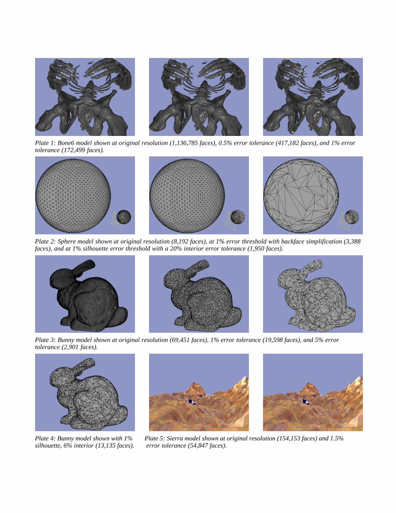
Plate 1: Bone6 model shown at original resolution (1,136,785 faces), 0.5% error tolerance (417,182 faces), and 1% errortolerance (172,499 faces).

Plate 2: Sphere model shown at original resolution (8,192 faces), at 1% error threshold with backface simplification (3,388faces), and at 1% silhouette error threshold with a 20% interior error tolerance (1,950 faces).

Plate 3: Bunny model shown at original resolution (69,451 faces), 1% error tolerance (19,598 faces), and 5% errortolerance (2,901 faces).

Plate 4: Bunny model shown with 1% Plate 5: Sierra model shown at original resolution (154,153 faces) and 1.5%silhouette, 6% interior (13,135 faces). error tolerance (54,847 faces).

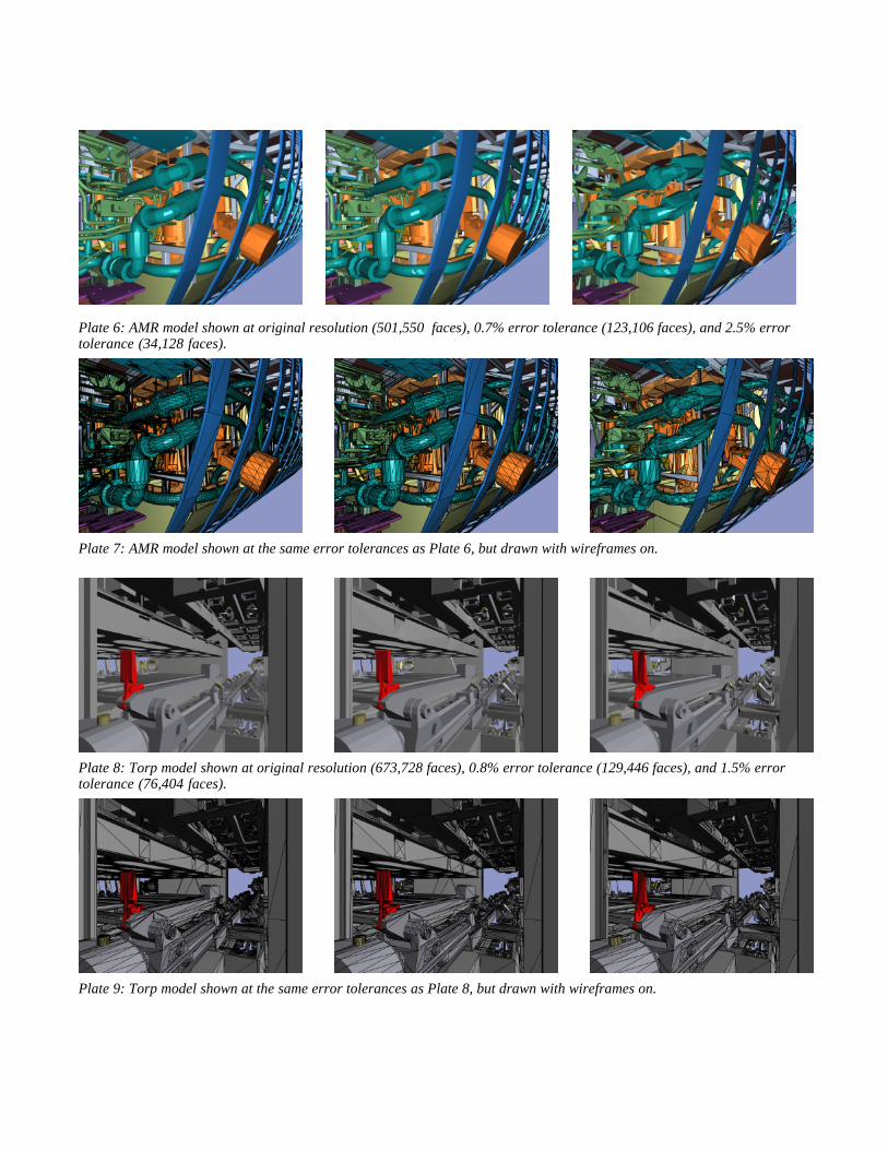
Plate 6: AMR model shown at original resolution (501,550 faces), 0.7% error tolerance (123,106 faces), and 2.5% errortolerance (34,128 faces).

Plate 7: AMR model shown at the same error tolerances as Plate 6, but drawn with wireframes on.

Plate 8: Torp model shown at original resolution (673,728 faces), 0.8% error tolerance (129,446 faces), and 1.5% errortolerance (76,404 faces).

Plate 9: Torp model shown at the same error tolerances as Plate 8, but drawn with wireframes on.