Embed Size (px)
Citation preview

VIEW COHERENCE ACCELERATION
FOR RAY TRACED ANIMATION
by
Philip Glen Gage
B.S., University of Colorado at Colorado Springs, 1983
A thesis submitted to the Graduate Faculty of the
University of Colorado at Colorado Springs
in partial fulfillment of the
requirements for the degree of
Master of Science
Department of Computer Science
2002

ii
This thesis for the Master of Science degree by
Philip Glen Gage
has been approved for the
Department of Computer Science
by
____________________________________Sudhanshu K. Semwal, Chair
____________________________________Marijke F. Augusteijn
____________________________________C. H. Edward Chow
__________Date

iii
Gage, Philip Glen (M.S., Computer Science)
View Coherence Acceleration for Ray Traced Animation
Thesis directed by Professor Sudhanshu K. Semwal
Ray tracing generates realistic images but is computationally intensive,
especially for animation. Many techniques have been developed to accelerate ray
tracing, including exploitation of temporal coherence between successive frames to
accelerate animation. This thesis extends earlier work on ray traced animation to add
efficient pan and zoom from a fixed viewpoint and other capabilities. A generalized
ray tracing method that integrates an object animation acceleration technique by
David Jevans with the new pan and zoom algorithms is presented, providing
accelerated object animation and field of view changes by maximizing reuse of
previous frame data. The algorithms were implemented in Java for both animation
and virtual reality interaction and results are presented showing an order of magnitude
performance improvement for typical pan and zoom operations.

iv
CONTENTS
CHAPTER
INTRODUCTION......................................................................................................1
PREVIOUS WORK.................................................................................................4
Ray Tracing........................................................................................................5
Geometry.......................................................................................................6
Shading..........................................................................................................8
Aliasing.........................................................................................................9
Extending ray tracing limitations................................................................10
Acceleration.....................................................................................................11
Bounding volumes......................................................................................12
Spatial subdivision......................................................................................13
Other techniques.........................................................................................16
Animation........................................................................................................18
Image Space versus Object Space...............................................................18
Object Space Temporal Coherence (OSTC)...............................................20
Interaction........................................................................................................22
DESIGN...................................................................................................................24
New Pan Animation (Panimation) Algorithm.................................................25
Standard viewing projection.......................................................................26

v
Cylindrical viewing projection....................................................................28
New Zoom Ray Sample Viewport (RSVP) Algorithm....................................32
Viewports....................................................................................................33
Integrating the Algorithms...............................................................................35
Algorithm Summary...................................................................................36
Integrating OSTC and RSVP......................................................................37
Integrating Panimation and RSVP..............................................................37
Integrating OSTC and Panimation..............................................................40
IMPLEMENTATION............................................................................................41
Development Process.......................................................................................41
Java..............................................................................................................41
Ray Tracer...................................................................................................42
Uniform Spatial Subdivision Grid..............................................................43
Temporal Coherence Animation Acceleration............................................44
Pan and Zoom.............................................................................................45
Java Classes.....................................................................................................45
The Panimation camera...............................................................................46
The Ray Sample Viewport (RSVP)............................................................50
Lights, Cameras, Action!............................................................................51
RESULTS................................................................................................................54
Animation....................................................................................................54
Virtual reality..............................................................................................58
FUTURE WORK....................................................................................................60

vi
Autopan and Autozoom..............................................................................60
View projections.........................................................................................62
Command language.....................................................................................62
Interaction...................................................................................................63
Compression................................................................................................63
Postprocessing.............................................................................................64
Testing.........................................................................................................64
Cached image blocks...................................................................................64
Spatial subdivision......................................................................................65
Generalized acceleration.............................................................................66
CONCLUSION.......................................................................................................68
BIBLIOGRAPHY...................................................................................................69
APPENDIX A. PROGRAMMER’S REFERENCE...........................................74
Operation.....................................................................................................74
Examples.....................................................................................................75

vii
TABLES
Table
Table 1. Animation Acceleration Algorithms.............................................................25
Table 2. Class Names and Descriptions......................................................................53
Table 3. Acceleration Results.....................................................................................55

viii
FIGURES
Figure
Figure 1. Example Ray Traced Image..........................................................................5
Figure 2. Ray Tracing Geometry..................................................................................7
Figure 3. Whitted Ray Tracing Shading Equation........................................................9
Figure 4. Uniform Spatial Subdivision Grid...............................................................13
Figure 5. Moving Object Shadow and Reflection......................................................19
Figure 6. Object Space Temporal Coherence.............................................................21
Figure 7. Pan by Image Shift and Retrace..................................................................26
Figure 8. Standard View Projection............................................................................27
Figure 9. Spherical View Projection...........................................................................28
Figure 10. Cylindrical Equirectangular View Projection...........................................29
Figure 11. Standard and Cylindrical Projections........................................................31
Figure 12. Zoom 2:1 Mapping....................................................................................32
Figure 13. Example Viewports...................................................................................34
Figure 14. Cylindrical Projection and Inverse............................................................37
Figure 15. Integrated Panimation and RSVP Algorithms...........................................38
Figure 16. Correcting Cylindrical Distortion..............................................................39
Figure 17. Class Hierarchy.........................................................................................46
Figure 18. Camera panImage Method........................................................................48

ix
Figure 19. Camera panImage Geometry.....................................................................48
Figure 20. Render Area Pseudocode...........................................................................49
Figure 21. Camera Render Pseudocode......................................................................50
Figure 22. Viewport Render Pseudocode...................................................................51
Figure 23. World Data Structure.................................................................................52
Figure 24. World Animate Pseudocode......................................................................52
Figure 25. Simultaneous Pan and Animation Image..................................................56
Figure 26. Camera and Viewport Images...................................................................57
Figure 27. Interactive Camera and Viewport Windows.............................................59
Figure 28. Viewport Autopan and Autozoom.............................................................60
Figure 29. View Frustrum Grid..................................................................................66

CHAPTER I
INTRODUCTION
Computer graphics is widely used in applications including advertising, art,
video games, data visualization, and recently, full-length motion pictures. Advances
in realistic rendering make it difficult to determine whether some images are real or
computer-generated. In a few years, computer-generated images may be almost
indistinguishable from reality.
Ray tracing is an elegant computer graphics technique that produces realistic
images, but runs slowly due to the extensive calculations required. Newer, faster
computers and better algorithms support more complex image generation. Even low-
end PCs are now capable of rendering not only single images, but long animations
composed of thousands of images, called frames. Users push the limits towards
greater scene complexity and realism, so there is always a need for more speed and
improved ray tracing acceleration schemes.
The two main research areas in computer graphics are realism and speed.
There is a tradeoff between the two, but careful optimization can improve efficiency
while retaining realism. The focus of this thesis is accelerating the ray tracing
animation process without sacrificing image quality.

2
Ray tracing can be used to generate animation sequences by rendering each
frame separately, but there are opportunities for performance improvement. Many
acceleration methods have been used to speed up ray tracing of still images, including
bounding volumes, spatial subdivision and ray coherence. Temporal coherence can
be used to accelerate ray traced interaction and animation by reusing data from one
frame to the next.
Jevans [JEVA92] presents an elegant method for accelerating ray traced
animation using object space temporal coherence (called OSTC here) to track the
image areas that need to be updated for each frame. This OSTC method and similar
approaches handle moving objects well, but require a static field of view. The
purpose of this thesis is to study such methods for accelerating ray tracing using
frame coherence, and to extend these techniques to allow useful dynamic camera
view transformations, including panning and zooming, from a fixed viewpoint.
Unfortunately, these acceleration methods do not allow the viewpoint to move
through the scene without a full image redraw, but the camera field of view can be
changed with fast partial image redraw.
If these pan and zoom changes are gradual, as they usually are, then most of
the image data from each frame can be reused in the next frame, redrawing only the
minimum screen area necessary as new parts of the scene come into view. Thus,
slow pan and zoom effects can be added to animations with only a slight increase in
execution time. In most previous approaches, performing pan or zoom requires
redrawing the entire image, greatly increasing execution time and interfering with
some acceleration schemes, including OSTC. The new pan and zoom algorithms

3
developed in this thesis allow pan and zoom to be used efficiently where in earlier
approaches such camera view changes might have been avoided.
The new algorithms can be used separately or combined with other algorithms
such as OSTC. The OSTC technique and the new algorithms operate similarly,
retracing only changed screen areas by reusing previous frame data for unchanged
areas. Object animation is accelerated by OSTC and camera view changes are
accelerated by the new pan and zoom algorithms. The combined system allows
simultaneous object animation, pan, zoom and other effects while updating only
changed areas of the screen. For sequences involving limited animation, pan or
zoom, only a small fraction of the pixels for each successive frame may need to be
ray traced, greatly reducing execution time.
The new algorithms were tested and verified by implementing a ray tracer in
Java similar to OSTC and extending the ray tracer to accelerate pan and zoom both
for animation and virtual reality (VR) interaction. Results indicate an order of
magnitude improvement in execution time for typical pan and zoom operations.
Chapter II describes the history and theory of ray tracing and animation
acceleration. Chapter III explains the rationale and design of the new pan and zoom
algorithms. Chapter IV discusses the Java implementation details. Chapter V
presents performance results and example images. Chapter VI contains ideas for
possible future work. Chapter VII is the final summary and conclusion.

CHAPTER II
PREVIOUS WORK
Rendering is the process of image synthesis, typically the projection of 3D
virtual models onto 2D images. Early graphics systems displayed wire-frame
renderings of 3D polygonal scenes, in which the edges of all polygons are drawn as
lines. However, such images show lines on the back sides of objects which should be
hidden. To produce more realistic images other rendering algorithms were
developed, including back-face removal, depth-sorting, area-subdivision, scan-line, z-
buffer and ray tracing methods [FOLE96].
An important issue in rendering is visible surface determination, also called
hidden surface elimination. The color of each image pixel is determined by the
closest opaque object in the view direction for the pixel. Finding the closest surface
implies a sorting process, which can be handled in many ways according to two
general strategies. Image-precision algorithms, such as ray tracing, find the closest
surface for each pixel, while object-precision algorithms find the visible pixels for
each object [FOLE96]. Typical graphics systems use an object-precision, pipelined
z-buffer method, which is fast but has limited shading capabilities in comparison to
ray tracing. Theoretically, ray tracing may someday become as fast as the z-buffer
method [WALD01].

5
Ray Tracing
Ray tracing is an elegant rendering algorithm that provides great versatility
and realism. The paths of light rays are traced mathematically to determine the color
of each image pixel. Shadows, reflection, refraction and other interesting optical
effects are easily supported. Reflection and refraction are handled recursively,
producing a tree of rays that contribute to the color of each pixel. Ray casting usually
refers to nonrecursive ray tracing without reflection or refraction, although some
authors treat the terms as synonymous. Figure 1 shows a ray traced image rendered
by the Java code developed for this thesis.
Figure 1. Example Ray Traced Image
Ray tracing has been used in art and optics for centuries [GLAS89]. In 1637
Descartes used ray tracing to explain how the shape of a rainbow is caused by light
refraction in raindrops. Artists used rays to develop perspective drawing techniques.
Rays were traced on paper to model the paths of light rays through systems with

6
lenses, mirrors and prisms. Computers are now used instead of paper to model the
design of telescopes and other optical instruments.
Appel [APPE68] was the first to use ray tracing for computer graphics, for
shading and shadows. He used a limited ray tracing technique to produce
architectural diagrams on a pen plotter. Whitted [WHIT80] was the first to describe
the complete ray tracing algorithm, combining earlier separate techniques for visible
surface determination, shadows, reflection and refraction in a single elegant method.
His paper forms the foundation of modern ray tracing and suggested many ideas later
pursued by other investigators.
Geometry
Some mathematical terminology is necessary to understand ray tracing. The
3D coordinate system has X, Y and Z axes perpendicular to each other. Each point
has an (x,y,z) location in this coordinate system. A vector has (x,y,z) coordinates that
represent a direction. The length of a vector is called its magnitude, and unit vectors
are normalized to a magnitude of one. A surface normal vector represents the
direction perpendicular to a surface at a given point. Two vector multiplication
operators are defined, the dot product and cross product. The dot product of two unit
vectors is the cosine of the angle between them. The cross product of two unit
vectors gives a vector perpendicular to both. A ray has an origin point and a direction
vector.
Figure 2 shows an example of ray tracing geometry. A fixed point is chosen
for the center of projection, called the eye or camera. A view direction vector points

7
in the direction the camera is looking. An imaginary image plane perpendicular to
the view vector represents the image pixels. Primary rays are traced from the camera
through the center of each pixel in the image plane into the 3D scene. This
arrangement defines the viewing projection that determines how 3D locations are
projected onto the 2D image plane. The process is backwards from actual photon
motion, but saves time by tracing only rays that contribute to the image.
Eye
Image Plane
Pixel
Normal
Reflection Ray
Transmission Ray
Light Sources
Object
Shadow Rays
IntersectionPoint
Figure 2. Ray Tracing Geometry
Each primary ray is algebraically tested for intersection with objects in the
scene, the closest intersection is the object visible at that pixel. Once the closest
intersection point is found, secondary rays, called illumination or shadow rays, are

8
traced to each light source. If a shadow ray intersects any object closer than the light
source, the object intersection point is in shadow with respect to that light, otherwise
the light intensity is included in the shading calculation. If the object is reflective or
transmissive (refractive), additional secondary rays for reflection or refraction are
traced recursively and included in the shading.
Shading
Shading is performed by accumulating the total light intensity at the
intersection point and combining with the object color at the point to obtain the pixel
color. Several illumination models have been developed with varying levels of
realism [FOLE96]. The Lambert cosine law defines the intensity coefficient as the
cosine of the angle between the surface normal and the light source direction, which
can be computed using the vector dot product. The Gouraud shading model
interpolates polygon vertex colors, while the Phong model interpolates vertex
normals and adds a specular exponent.
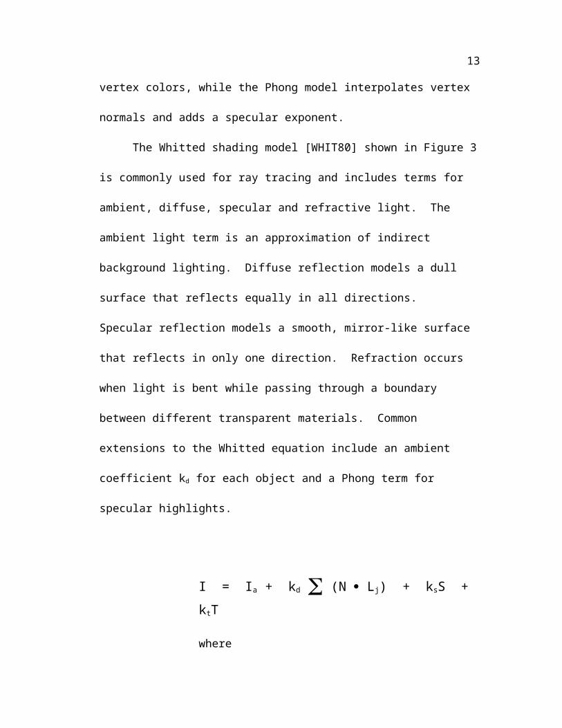
The Whitted shading model [WHIT80] shown in Figure 3 is commonly used
for ray tracing and includes terms for ambient, diffuse, specular and refractive light.
The ambient light term is an approximation of indirect background lighting. Diffuse
reflection models a dull surface that reflects equally in all directions. Specular
reflection models a smooth, mirror-like surface that reflects in only one direction.
Refraction occurs when light is bent while passing through a boundary between
different transparent materials. Common extensions to the Whitted equation include
an ambient coefficient kd for each object and a Phong term for specular highlights.

9
I = Ia + kd (N Lj) + ksS + ktT
whereI = total reflected intensityIa = ambient light intensitykd = diffuse reflection coefficientN = surface normal vectorLj = direction of jth light sourceks = specular reflection coefficientS = reflected light intensitykt = transmission coefficientT = transmitted light intensity
Figure 3. Whitted Ray Tracing Shading Equation
Aliasing
Aliasing is an undesirable phenomenon caused by digital undersampling of an
analog signal which causes high frequencies to alias as lower frequencies. Pixels are
digital samples of continuous shapes and show spatial aliasing defects such as jagged
edges, called “jaggies”. Animation frames are digital samples over time and have
temporal aliasing artifacts such as rotating wheels appearing to spin backwards.
Antialiasing methods sample the signal at higher frequencies to reduce
aliasing errors. The ray tracing approach for antialiasing is to fire several primary
rays through each pixel and average the results. Distributing several rays across the
area of a pixel may hit multiple objects that partially cover the pixel, resulting in a
blended color that more closely approximates the correct value. Whitted [WHIT80]

10
describes adaptive supersampling, a technique that shoots more rays in areas of
varying color to reduce aliasing errors caused by undersampling.
Extending ray tracing limitations
Cook [COOK84] extended the antialiasing technique to distributed ray
tracing. His terminology is unfortunate, since it suggests distributed processes across
a computer network but really refers to rays distributed in space or time. The method
is usually called distribution (or stochastic) ray tracing now to avoid confusion. It
extends supersampling to produce several useful effects, including motion blur,
penumbra (soft shadows), gloss (blurred reflection), translucency (blurred refraction)
and depth of field (blurred focus). Parameters such as angle, location and time are
varied, or “jittered,” for each ray and several rays are averaged together for each
pixel.
The popular early 1980s ray traced images of reflective spheres on
checkerboards represented a startling jump in realism compared to earlier techniques.
However, ray traced images tend to look “too real,” with sharp shadows and
reflections. Distribution ray tracing helps make more realistic images, with real-
world blur and fuzziness.
The use of infinitesimally thin rays is another weakness of ray tracing and
does not model the real world well. Antialiasing and distribution ray tracing reduce
this problem by using several rays statistically instead of just one sample. Another
approach is the use of generalized rays, bundles of rays or wider rays, including

11
beam, cone and pencil tracing [GLAS89]. Monte Carlo ray tracing and path tracing
[JENS01] have also been used to distribute rays statistically.
With Whitted’s recursive algorithm, supersampled antialiasing and Cook’s
distribution algorithm, ray tracing is a powerful rendering method. However,
traditional ray tracing does not handle some optical phenomena, such as global
illumination (interreflectance) and caustics [WATT92]. Global illumination refers to
light bouncing around the scene, such as color “bleeding” onto nearby objects, and
gives soft, realistic lighting to a scene. Caustics are irregular bands of light reflected
off specular surfaces or distorted refraction such as sunlight through water. These
effects cannot be modeled by traditional means of tracing rays backwards, but require
forward tracing.
Several methods, including bidirectional ray tracing [ARVO86], radiosity
[WATT92] and photon mapping [JENS01] have been used to extend ray tracing to
include such effects. Ray traced images look impressive but do not model light as
accurately as radiosity by not accounting for some illumination effects, such as
caustics. Hybrid methods that combine ray tracing with global illumination modeling
hold the promise of greater realism in the future, but are currently too complex and
slow for wide use.
Acceleration
Ray tracing is slow since a typical image may require tracing millions of light
vectors. The majority of time in a ray tracer is spent intersecting rays with objects.
In an often-quoted statistic, Whitted [WHIT80] estimates that ray-object intersection

12
tests may take over 95% of execution time for complex scenes. The traditional brute-
force approach tests every ray with every object for possible intersections.
Many techniques have been developed to speed up ray tracing [GLAS89,
SHIR00], some of these involve complex algorithms and data structures. Most
acceleration schemes reduce the number of intersection tests by skipping cases where
it can be determined that the ray cannot intersect the object. Arvo and Kirk
[GLAS80] divide ray tracing acceleration methods into faster/fewer intersections,
fewer rays and generalized rays. Custom hardware and parallel processing [PARK99,
REIN00] have also been used and ray tracing is easy to parallelize, unlike some
algorithms.
Bounding volumes
The bounding volume technique was described by Whitted in his classic paper
[WHIT80]. A bounding volume is a simple shape, usually a sphere or box, that
encloses a more complex object to provide a faster intersection test. If the ray does
not intersect the bounding volume, the intersection tests against the objects in the
volume can be skipped. This can save significant time for complex algebraic surfaces
or composite objects composed of many smaller objects.
Even greater savings are provided by bounding volume hierarchies, which
group sets of bounding volumes and objects inside larger bounding volumes. Each
ray is tested for intersection with the outermost volumes. Only if the ray hits the
volume is it tested against inner volumes and objects recursively.

13
Spatial subdivision
Another approach is spatial subdivision, which partitions the scene into a grid
of volumes called voxels. The voxels may be uniform or nonuniform size. Figure 4
illustrates a uniform spatial subdivision grid. Each voxel has a list of the objects that
are contained in it or intersect it. An object may intersect one or many voxels. Rays
are propagated along their paths from voxel to voxel, checking for intersections with
the object list in each voxel. This restricts the object intersection tests to only objects
near the ray’s path. Also, the voxels are checked in nearest to farthest order, which
can further speed rendering of complex scenes with many densely clustered objects.
When an object intersection is found, it must be ignored if it is not in the current
voxel to avoid missing possible closer intersections with other objects. If a valid
intersection is found, the remaining objects in that voxel must still be checked in case
there is a closer intersection in that voxel.
Eye
Image Plane
Grid around Scene
Rays
Figure 4. Uniform Spatial Subdivision Grid

14
Glassner [GLAS84] used the octree structure for ray tracing spatial
subdivision. The scene volume is recursively divided into 8 sub-volumes called
octants until there are less than a maximum number of objects intersecting each
voxel. This results in a nonuniform subdivision that has smaller voxels in areas with
more objects. He notes that spatial subdivision always saves time unless grid
traversal is very slow.
Fujimoto [FUJI86] compares uniform and octree spatial subdivision in a
hybrid method called Accelerated Ray-Tracing System (ARTS). A 3D digital
differential analyzer (3DDDA) traversal algorithm is defined to propagate rays
through voxels, based on Bresenham’s famous 2D line generator. The approach is
rather complex and later papers simplify the uniform subdivision traversal.
Amanatides and Woo [AMAN87] compare bounding volume and spatial
subdivision methods. Bounding volumes take less memory, while spatial subdivision
has easier grid traversal. Unlike the Fujimoto 3DDDA, their traversal has no required
dominant axis that is always incremented. They note that to check if an intersection
is inside the current voxel, the ray distance can be used instead of checking the six
voxel walls.
Cleary and Wyvill [CLEA88] describe a similar traversal method, claiming
that uniform spatial subdivision is typically faster than nonuniform adaptive
subdivision and only a few hundred voxels are usually needed. They note that
polygon intersection tests can be limited to edges inside the voxel.
Jevans and Wyvill [JEVA89] recursively subdivide voxels into a hierarchy of
nested grids. The algorithm is parameterized to act as octree, uniform or adaptive.

15
They use the Cleary [CLEA88] voxel traversal with a more compact XYZ array
notation, and a 1D voxel array instead of 3D for faster indexing performance.
Reinhard [REIN00] presents two useful ideas for spatial subdivision. If an
object moves outside the grid, it can be wrapped to a larger logical grid size to avoid
rebuilding the whole grid. The locations of such objects are wrapped to fall within a
voxel and tagged as wrapped. A larger logical grid space is traversed by wrapped
rays using the original grid as a hash table to store objects outside the grid. He also
describes an octree-style structure that allows objects at any level, not just leaf nodes.
This provides fast insertion and deletion of large objects at higher level nodes. The
leaf nodes are traversed and parent nodes are searched up the tree and tagged with the
ray ID.
Glassner [GLAS89] uses a space-time approach that considers moving 3D
objects as static 4D objects intersected by 4D rays. A hybrid bounding volume and
spatial subdivision method is used. Motion blur is easily handled by varying the ray
start times.
Several authors [AMAN87, SEMW87, CLEA88, JEVA89] note the
“mailbox” or ray ID technique. Multiple intersection tests of a ray with the same
object can be avoided by saving the ray ID from each intersection in each object and
checking this ID before intersection. If the ray ID matches, the ray has already been
intersected with the object in an earlier voxel and the saved intersection data can be
used.
Semwal [SEMW87] describes a spatial subdivision method called the Slicing
Extent Technique (SET). Axis-aligned planes, or slices, are used to bound each

16
object. The intersection of slices creates rectangles, or cells, on each slice. Each 2D
cell has a list of associated objects, and each object is associated with at least 6 cells
that surround it. During ray traversal the object list of each encountered cell is tested
for possible intersections. A large number of objects may create too many cells to
handle effectively. To avoid SET limitations, the Modified SET (MSET) method was
developed [LOGA89]. MSET uses a uniform spatial grid that supports a large
number of objects and allows easy traversal by incrementing through evenly-spaced
slices. Each cell has “up” and “down” lists for objects on either side of the cell.
Unlike most grid methods, 2D cells are used instead of 3D voxels. A benefit is that
no duplicate ray-object intersection tests are performed because each object is
assigned only to cells on six slices surrounding the object.
Other techniques
Directional techniques [GLAS89] such as light buffers, ray coherence, ray
classification and proximity clouds make use of direction during the preprocessing
voxel build. They use a directional cube with six faces that may be subdivided. Each
face has a list of objects which lie in that face’s direction, allowing rays to be checked
for intersection with smaller lists of objects based on the ray’s direction. The ray
classification method [ARVO87] uses 5D representations of rays and bounding
volumes, extending space subdivision to include ray direction. The 5D rays (origin
and two direction angles) are compared with 5D partitions to retrieve presorted lists
of candidate objects for intersection tests.
17
Coherence refers to local similarity, or smooth, gradual change in space or
time. Nearby things tend to have similar properties, which provides opportunities for
acceleration. There are dozens of names for various types of coherence, but they all
involve spatiotemporal locality. Spatial coherence refers to 3D object space, while
image coherence follows from this because the same objects are projected onto 2D
image space. Ray coherence provides acceleration by processing generalized bundles
of rays together and includes methods such as beam, cone and pencil tracing
[GLAS89]. Temporal coherence uses spatial or image similarities between adjacent
animation frames in the time domain. Memory coherence [PHAR97, WALD01] is a
recent development that is not based on scene geometry, but reorganizes algorithms
and data structures to improve CPU instruction pipelining and memory cache
performance for modern computer architecture. This thesis focuses on image space
view coherence, using temporal coherence for field of view changes from a fixed
camera location.
Reprojection [ADEL95, WALD01] is an object space view coherence method
using image-based rendering (IBR) that allows pixels to be reused after camera
location changes. The previous frame pixels are projected onto the new view plane
using 3D geometry. This requires the pixel Z depth or distance to be saved during ray
tracing so the 3D transform to the new viewpoint can be performed, along with other
data such as surface normal and diffuse color. Intersection tests are performed to
detect possible intervening objects, if none, the reused pixel is reshaded as needed for
reflection and refraction. Due to geometric inaccuracy, this method can lead to image
errors but Adelson [ADEL95] describes how exact sub-pixel accuracy can be

18
maintained and all types of animation change can be handled. Light source changes
are problematic and the method requires a large amount of memory.
Animation
Animation gives a feeling of realism and life to still images by adding motion.
The human eye sees the appearance of continuous motion when a series of images are
shown in rapid succession at around 20 frames per second or faster. To produce
animation, the attributes of some of the objects in the scene are changed slightly from
frame to frame. These attributes include position, rotation, size, shape, color, texture
and other features. In addition, the position and color of light sources and the camera
field of view may be changed between frames.
Typically, most of the pixels in a frame are the same as in the previous frame,
with changes localized to a few areas where objects are moving, and the shadows and
reflections of these moving objects. Simple ray tracers regenerate the entire image
for each frame, ignoring the potential acceleration benefits of frame coherence. Much
time could be saved by reusing the unchanged pixels or saved rays from the previous
frame and ray tracing only the changed pixels. Animations can be generated much
faster by fully rendering only the first frame and then only the pixels that are different
in each successive frame.
Image Space versus Object Space
Consider a single moving 3D object from one frame to the next, shown in
Figure 5. It is easy to determine the old and new locations of the object on the image

19
and redraw these pixels. However, it is difficult to determine which pixels are
affected by the object’s shadow, reflection and refraction.
Figure 5. Moving Object Shadow and Reflection
To handle these problems, two types of animation acceleration algorithms
have been developed, image space coherence and object space coherence. Image
space algorithms render some frames and interpolate in-between frames, but may
cause image errors. Object space algorithms track 3D changes and project these to
image pixels needing redraw, and generally do not cause image errors.
Chapman [CHAP90] presents an image space method similar to 2D morphing
for accelerating ray traced animation using temporal coherence. Ray tracing is
performed in 4D space-time, rendering a pixel across time in multiple frames. Every
n-th frame is rendered, where n is based on the maximum frequency at which pixels
are expected to change. For pixels that vary in color between these frames a binary
search is performed in the time domain to find the frame in which the color change
occurred. Once the pixel color is found for a range of frames, it is copied to the
corresponding pixel in all in-between frames. This scheme is simple and handles all

20
types of image change, but rapidly moving objects may be rendered incorrectly due to
aliasing if the value of n is set too large.
Murakami [MURA90] uses object space coherence with a static view to
accelerate ray tracing by redrawing only the changed parts of the image. The ray tree
for each pixel is saved, along with additional intersection data. A list of traversed
voxels is saved for each ray so that only rays passing through changed voxels are
updated. Changed pixels are detected by checking whether any ray in the tree passed
through a changed voxel. If so, the pixel is reshaded, reusing much of the previous
ray tree data. Applications involving animation, interaction and parallel processing
are discussed. The method is complex and requires a large amount of memory.
Object Space Temporal Coherence (OSTC)
Jevans [JEVA92] describes a simpler object space method using spatial
subdivision and temporal coherence to accelerate animations with a static camera
view. The data structure works backwards from the Murakami approach, each voxel
keeps track of rays that traversed through it. The mapping between changed pixels
and changed voxels can be done in different ways. Jevans uses a spatial subdivision
grid in which each voxel has an associated 16x16 bitmap that represents the 256
corresponding sections of the image plane, independent of image resolution.
Each ray is tagged with the image area index of its origin. The bit
corresponding to the image area is set in each traversed voxel’s bitmap as the ray
moves through the scene. Each voxel then contains a bitmap of which screen areas
are dependent on rays passing through the voxel. These voxel bitmaps are populated

21
when the first frame is fully traced, and updated for changes on subsequent frames.
Both primary and secondary rays are included in the bitmap, so the technique
correctly handles shadows, reflection and refraction. When the scene changes, the
bitmaps of changed voxels are checked to determine which image areas are affected
and only those areas are recomputed. This can greatly accelerate image generation,
since only the rays for image areas in which changes have occurred need to be
recalculated. This OSTC technique is shown in Figure 6.
Eye
Spatial Subdivision Voxel Grid
Rays
Image Areas
0 0
1
11
0
0
0
0 0
0
0
0
0
0
0
Rays setimage areabit in eachtraversedvoxel bitmap
Figure 6. Object Space Temporal Coherence
The Jevans method handles object animation well and can handle light source
animation also, but less efficiently since changing a light typically affects most of the
image. If a light is moved or changes color, only the image areas that are in shadow

22
from both the old and new light location will not be retraced. He suggests keeping
the shadow rays in a separate bit set in each voxel to improve light animation
performance.
Jevans allows no camera motion in his algorithm and presents an analysis
showing the high percentage of static camera shots in an example set of animations.
Improving this static camera limitation is the major motivation of this thesis.
Interaction
The fast ray tracing capabilities needed for animation can also be used for
interactive scene changes to a previously rendered image. Either a human operator or
an algorithm (e.g., a simulator or video game) can drive the interaction. Potential
uses include scene editing, virtual reality, video games and simulators.
Sequin [SEQU89] describes a ray tracing method that allows light source and
object surface colors to be changed and rendered interactively. For each pixel, a
parameterized expression that includes light intensities and surface properties
contributing to the pixel’s color is saved during the initial ray tracing. Then the user
can interactively modify light and surface colors with the results displayed in a few
seconds by reevaluating the expressions. This method does not allow motion or other
geometry changes in the scene.
Briere [BRIE96] presents a more advanced approach that allows both color
and geometry changes, but requires more complex data structures and algorithms.
Saved ray trees and color trees are used to retrace changed parts of an image after

23
interactive update. The ray trees save visibility data to accelerate geometry changes,
while the color trees save shading data for light source changes.
Parker [PARK99] discusses interactive ray tracing using multiprocessing with
60 parallel processors, allowing the user to move the camera viewpoint while
rendering fairly complex scenes with interactive frame update rates. Such fast
hardware schemes are beyond the scope of this thesis, which concentrates on software
acceleration methods for single processor systems.

CHAPTER III
DESIGN
This section explains the design philosophy for the new pan and zoom
algorithms. Image space acceleration algorithms, such as Chapman [CHAP90],
handle object animation but are limited by 2D interpolation, require a static camera
and may cause image errors. Object space algorithms such as the Murakami
[MURA90] and Jevans [JEVA92] methods accelerate light and object animation, but
require a static camera. The reprojection method [ADEL95, WALD01] handles
camera motion but is complex, requires a large amount of saved data and may cause
image errors.
Reprojection could be simplified to support only pan and zoom without
allowing the camera to move through the scene. However, this would be a trivial
simplification of a well-established, more general method. This thesis pursues a new
and completely different approach to accelerating pan and zoom.
Table 1 shows a rough categorization of animation acceleration algorithms
with the two approaches: image and object space, and the three types of change: light,
object and view. Image space algorithms tend to be simpler but less accurate. This
classification is not precise or complete, but is intended to show that there is a lack of
image space view acceleration algorithms. This thesis explores new algorithms to fill
this apparent gap in animation acceleration techniques.

25
Image Space Object SpaceLights Saved light and surface
parameters [SEQU89]Saved ray trees [BRIE96]
Objects Frame interpolation [CHAP90]
Temporal coherence [MURA90, JEVA92]
View Pixel reprojection [ADEL95, WALD01]
Table 1. Animation Acceleration Algorithms
There seems to be a need for a simple image space method to support field of
view changes without retracing the entire image. There is much coherence during
slow view changes such as pan and zoom. These slight changes cannot be handled by
most animation acceleration algorithms, which require exact alignment between
frames to determine differences. This suggests that new image space techniques
might be effective to handle field of view changes separately, and could be added to
any ray tracer and animation acceleration scheme.
New Pan Animation (Panimation) Algorithm
The obvious way to reuse previous frame data and accelerate pan is to shift
the image and redraw only the newly exposed area. For example, to pan right, the
image could be shifted left by the appropriate amount and the newly visible area at
the right could be ray traced. Typically, the new area scrolling into view is a small
fraction of the image and only a few rows or columns of pixels need to be traced. In
this way, slow pan can be performed with little increase in execution time.

26
Figure 7 shows the new shift and retrace technique, called the Panimation
algorithm. Simultaneous horizontal and vertical pan can be performed by shifting the
image once diagonally. Care should be taken that the newly exposed corner where
the new horizontal and vertical areas overlap is not updated twice but only once.
Figure 7. Pan by Image Shift and Retrace
Standard viewing projection
Unfortunately, this pan by shift idea fails with the standard viewing projection
used in ray tracing because the view angle varies per pixel. The standard view
projection geometry is shown simplified to 2D in Figure 8. The advantage of this
projection is that straight lines in the scene appear straight in the image [EBER01].

27
The flat rectangular view plane causes pixels near the edge of the image to cover less
angular area than pixels near the center, causing objects near the edge to appear
squashed if a wide field of view is used. This is a common problem in film
photography with wide angle lenses also, since the film is the same kind of flat
rectangular view plane used in ray tracing.
Eye
Image plane with equally spaced pixels
Unequal angles
Figure 8. Standard View Projection
Because the image plane grid is evenly spaced, rays from the eye make
increasingly smaller angles near the edge. Since a pixel near an image edge
represents a smaller view angle, it is equivalent to a higher resolution than near the
image center. This means that pixels cannot be shifted away from center toward an
edge, or lower resolution data would be used to replace higher resolution data,

28
causing image degradation. This greatly complicates using pixel shift to accelerate
pan with a standard view projection. This is a major problem with the Panimation
approach, and probably the reason it has apparently not been used before. The
problem can be avoided if the viewing projection uses equal angular area per pixel
across the field of view. To allow panning, pixels must cover an equal angle in both
directions, implying a spherical projection with equal angle pixels in both azimuth
and elevation as shown simplified to 2D in Figure 9.
Equal anglesEye
Image plane with unequally spaced pixels
Figure 9. Spherical View Projection
Cylindrical viewing projection
Similar projections are widely used for geographic world maps [PAET90],
and several were studied for this application. A spherical surface like the world or the

29
imaginary “celestial sphere” seen by an observer cannot be mapped to a flat surface
without distortion. The type of distortion varies depending on the projection used.
The Cylindrical Equirectangular projection [MUSG92] shown in Figure 10
was selected as a suitable technique. The eye is at the center of a virtual sphere
enclosed in a cylinder. This is a trivial map projection of spherical latitude/longitude
points onto an infinite height cylinder of Earth radius centered along the north/south
pole axis and tangent at the equator. The cylinder is unrolled to form a flat
rectangular map that can include the entire earth surface or a smaller area. Since the
cylinder is tangent to the earth sphere, the tan function can be used to compute
coordinates along both axes up to 180 degrees. Using the sin and cos functions to
compute points around the equator extends the horizontal field of view to 360
degrees. This projection has singularities at the north and south poles so the
displayed latitude cannot quite reach the –90 or 90 degree values.
Eye
Object
ProjectedPoint
Longitude (azimuth)
Latitude (elevation)
90
-90-180 180
World Map(panoramic view)
45
0
-45
-90 0 90
Unroll Cylinder
North
South
Figure 10. Cylindrical Equirectangular View Projection

30
Using this cylindrical projection or a similar equal-angle method allows pan to
be emulated by image shift, since each pixel represents an equal area of the viewing
sphere centered at the observer. Latitude and longitude correspond to the elevation
and azimuth of the camera view ray. Moving a window on this virtual world map is
equivalent to pan, and resizing the window is zoom, since each pixel represents an
equal view angle. Vertical lines remain vertical in the image, like longitude lines
projected on the cylinder. But other lines may appear curved if a wide field of view is
used, in extreme cases following strange transcendental shapes [GLAE99].
A benefit is that the cylindrical projection allows a full 360 degrees azimuth
by 180 degrees elevation panorama view of the entire scene, while the standard
projection is limited to less than 180 degrees and has severe edge distortion at angles
much less than this. Angles greater than 360 degrees horizontal or 180 degrees
vertical produce a repeating periodic pattern.
This type of projection has some curvilinear distortion if a wide field of view
is used, but is similar to the standard viewing projection for a narrow field of view,
around 30 degrees or less. However, this may mean putting the eye point further
away from the scene, like a telescope or telephoto lens. This may cause problems
with objects blocking the view. The cylindrical distortion can be corrected as
explained later in this thesis (see section on Integration). Figure 11 compares the
standard and cylindrical projections with narrow 30 degree and wide 100 degree
fields of view. Both projections have noticeable distortion at wide angles, but the
type of distortion is different.

31
a) Standard Projection 30 Angle b) Standard Projection 100 Angle
c) Cylindrical Projection 30 Angle d) Cylindrical Projection 100 Angle
Figure 11. Standard and Cylindrical Projections
As the eye recedes an infinite distance from the image plane, both the
cylindrical and standard projections approach the same orthographic projection with
parallel rays. This indicates that the difference between the cylindrical and standard
projections is indeed reduced by narrowing the view angle, which can be confirmed
visually. The orthographic projection has equal-area pixels that work with the
Panimation algorithm, but gives no perspective effect for depth. Objects appear the
same size regardless of distance. This looks odd for typical ray tracing scenes, but is

32
useful in some application areas, such as computer-aided design (CAD) and data
visualization.
New Zoom Ray Sample Viewport (RSVP) Algorithm
The Panimation algorithm does not support accelerated zoom, although
zooming by an integer multiple n:1 or 1:n can be performed while reusing 1/n2 of the
pixels. If the zoom factor is 2 then ¼ of the pixels can be reused by mapping one
pixel to a 2x2 block in the other image. Figure 12 shows a simple example of this 2:1
mapping with a 16x16 pixel image. A single pixel can be used from each 2x2 block
(the upper left pixel in this example) or the four pixels could be averaged.
Figure 12. Zoom 2:1 Mapping
Zoomed out to wide angle Zoomed in to narrow angle
0 1 2 3
4 5 6 7
8 9 10 11
12 13 14 15
0 1 2 3
4 5 6 7
8 9 10 11
12 13 14 15

33
It would be useful to find a better zoom algorithm to allow smooth zoom at
any factor while reusing the maximum number of previous frame pixels and retracing
the minimum number of pixels for each frame. This is the same philosophy used in
developing the Panimation algorithm.
Consider zooming out to a slightly wider field of view. This could be
accomplished by rescaling the image smaller towards the center and ray tracing only
the new pixels around the edges of the image. However, after a few frames the scaled
image data would begin to degrade due to sampling and aliasing errors. Also, the
process is not reversible to zoom back in, because the original higher resolution
image data has not been preserved.
A better approach for zooming out is to draw the new pixels around the edges
of the image at the same resolution as the original image and resample the whole area
down to a lower resolution for each frame. This avoids degradation by performing a
single resampling of a higher resolution image to a lower resolution image for each
frame. The process is reversible, the view can be zoomed in until the original image
resolution is reached without ray tracing any new pixels in this case. This implies
that a frame buffer larger than the final image size is needed. This approach is called
the Ray Sample Viewport (RSVP) algorithm.
Viewports
The smaller image is a viewport onto a portion of the larger, and could be
considered another eye point and view plane as a second level of view projection, or
merely a 2D transform. The viewport algorithm itself allows any view projection to

34
be used, standard, cylindrical or other. As the viewport grows larger, not all pixels in
the parent camera frame buffer need to be ray traced since only some will be sampled,
assuming one sample per pixel and no color interpolation or antialiasing. This means
that full ray tracing of the entire larger frame buffer can be disabled with the viewport
requesting that individual scattered pixels be ray traced on demand as needed. The
number of traced pixels required is the smaller viewport size or less, not the larger
frame buffer size.
Pixel tracing on demand means that each pixel in the camera frame buffer
must be tagged whether it is current or needs to be retraced. Rather than allocate
more storage for these tags, a special null color value can be defined and used to
indicate invalid pixels. When temporal coherence or panning causes a screen region
to be marked as changed due to object movement or pan operations, the region is
overwritten with the null color. When a viewport samples a null color pixel, it is ray
traced. If the whole image ever needs to be updated, all null color pixels can be
retraced. Figure 13 shows a buffer with such viewports, which can be positioned,
rotated and warped as needed.
Ray Traced Camera Frame Buffer
Viewports
Viewport shapecan be rectangular or warped
Viewportscan overlap and be rotated
Figure 13. Example Viewports

35
Other useful effects are supported by the RSVP method. Rotate, scale, shear
and more unusual changes can be produced by simple 2D transforms. Any pattern of
pixels in the camera frame buffer can be resampled into the viewport image. This
could allow special effects normally done during postprocessing to be performed at
run time.
Multiple viewports can be attached to a single camera, each requesting a
different set of pixels from the same camera frame buffer. Some of these pixels may
already have been rendered by a previous overlapping viewport, so the camera frame
buffer acts as a pixel cache for all viewports on the camera. This can accelerate pan,
zoom and other transforms within the frame buffer view area. Thus, there may only
be a slight performance penalty for multiple overlapping viewports. Viewports can
be switched to different cameras as desired, or can sample multiple cameras
simultaneously for fade and multi-view effects.
Although the RSVP technique allows unlimited 2D image space transforms,
the range of motion is somewhat limited by the image buffer size. Pixels sampled off
the buffer edge could be set to black, or ray traced but not saved in the camera buffer
with a loss in caching efficiency. This suggests that the Panimation and RSVP
algorithms could be combined together for complementary functionality.
Integrating the Algorithms
Three main algorithms are used in this thesis, the Jevans OSTC animation
acceleration method [JEVA92], the new Panimation algorithm and the new RSVP
algorithm. These are different algorithms that may be used separately or together in

36
any combination and are easily added to most ray tracers. Each performs a different
type of acceleration, but they operate similarly and work well when integrated
together. A combined approach allows each algorithm to handle deficiencies in the
other algorithms and produces a more robust approach without many of the
weaknesses of the individual algorithms.
Algorithm Summary
The OSTC algorithm [JEVA92] tracks object (and possibly light) changes
during animation and uses a rectangular grid on the image to determine which areas
need retracing. Object animation is unlimited but a static camera must be used with
no panning or zooming.
The Panimation algorithm developed in this thesis accelerates panning by
shifting the previous image and ray tracing only the new area. This requires a
cylindrical equal-angle view projection that allows panoramic views but has curved
distortion at wide angles. Unlimited range of pan and zoom is supported with pan
greatly accelerated, but zoom can only be accelerated slightly by using an n:1 zoom
ratio and reusing 1/n2 pixels.
The Ray Sample Viewport (RSVP) algorithm developed in this thesis uses a
viewport to sample pixels from a ray traced buffer according to any 2D image
transform. RSVP accelerates pan, zoom, rotate and other effects but the range of
motion should be limited to the sample buffer area. If pixels are sampled off the
buffer area, they can be set to a default color such as black, causing an image defect,
or ray traced but not saved for reuse, causing potential decrease in acceleration.

37
Integrating OSTC and RSVP
Integrating the OSTC and RSVP algorithms is trivial. Instead of ray tracing
the OSTC updated image areas, they are erased to the null color. When a viewport
samples a null pixel, it is ray traced at that time.
Integrating Panimation and RSVP
Integrating the new Panimation and RSVP algorithms is similar, new areas
exposed by panning are drawn in the null color. The cylindrical projection must be
used to support accelerated pan, which introduces the cylindrical distortion problem.
An interesting benefit of integrating these two algorithms is that a viewport transform
can be used to undo the curved distortion of the cylindrical projection needed for
Panimation. Since the tan function is used for the cylindrical projection, the arctan
(or atan2) function can be used for the inverse transform, restoring the standard
projection appearance. This fixes a major problem with the Panimation algorithm.
Figure 14 shows the cylindrical projection geometry and equations. This integrated
Panimation/RSVP approach is shown in Figure 15.
Cylindrical Projection
x = sin(a)y = tan(e)z = cos(a)
Inverse Cylindrical Projection
a = arctan(x/z)e = arctan(y)
X
Y
Z
(x,y,z) (x,y,z)
a
e
a = azimuthe = elevation
Rectangular
Cylindrical
Figure 14. Cylindrical Projection and Inverse

38
Eye
Cylindrical EquidistantView Projection
Ray Traced PanimationImage Buffer with
Cylindrical Distortion
Ray SampleViewport(RSVP) without
Cylindrical Distortion
Transforms forpan, zoom, rotate,inverse cylindrical
& other effectsaccelerated bypixel caching
Pan accelerated by image shift,zoom 2:1 with1/4 pixel reuse
Panoramic WorldView Plane
Objects
Figure 15. Integrated Panimation and RSVP Algorithms
Panimation provides fast large-scale pan but causes unwanted curvilinear
distortion. Adding RSVP provides fast small-scale pan, zoom and other effects.
When a RSVP transform is used to correct the cylindrical distortion, the integrated
method gives accelerated pan, zoom and other features without the unwanted
distortion.
Figure 16 shows an image with the cylindrical distortion and the warped set of
viewport sample pixels that generated the resulting standard projection image with
the cylindrical distortion removed. The upper image is less distinct because only the

39
sampled pixels were ray traced. The straight lines in the checkerboard grid have been
restored in the corrected image, but the spheres exhibit stretching away from the
image center due to the wide 100 degree field of view. All view projections have
distortion of some kind, in this case cylindrical distortion has been traded for
rectangular distortion, which is more familiar and acceptable.
a.) 640x480 camera image sampled pixels
b.) 320x200 viewport image from sampled pixels
Figure 16. Correcting Cylindrical Distortion

40
Integrating OSTC and Panimation
To integrate the OSTC and new Panimation algorithms, rectangular image
areas invalidated by either algorithm are set to the null color. The pan is done first to
avoid wasting time by updating areas already scrolled off the image. To make the
temporal coherence bits refer to the same scene areas after pan, the cumulative pan
offset in pixels is saved and used to offset the bit areas.
The bit correspondence must be wrapped as the image is panned, so that bits
that represented areas now scrolled off the image are reused for new areas that scroll
onto the opposite side. An extra row and column of bits is allocated to handle partial
areas on both sides of the image. When a row or column is wrapped and reused, the
corresponding bits are cleared in all voxels to start collecting new data. After a
complete image buffer redraw, all bits are cleared in all voxels to start over.

CHAPTER IV
IMPLEMENTATION
The code developed for this thesis does not have robust error checking, full
OO encapsulation with get/set methods, extensive optimization or other
nonessentials. The intent is clarity and simplicity for testing new animation
acceleration algorithms. Not all features of a typical ray tracer are supported, but
could be added in the future as necessary.
Only a single ray per pixel is used, no pixel color interpolation, antialiasing or
distribution ray tracing is performed. Images may be sampled from higher to lower
resolution, but not vice-versa. The goal is generation of the same image produced by
full ray tracing while maximizing the reuse of previous frame pixels.
Development Process
Java
Java is a new object-oriented (OO) programming language that was selected
for the implementation. It supports classes, packages, multithreading, exception
handling, automatic garbage collection and many other features [ARNO98].
Libraries are provided for a wide range of functionality, including graphics. Java is
portable and runs on a bytecode interpreter instead of being compiled to native
machine code. The original Java interpreter seemed slow for number-crunching

42
applications like ray tracing, but newer just-in-time (JIT) compilers allow Java to run
almost as fast as compiled languages.
Java classes encapsulate methods (code) and fields (data). A Java object is an
instance of a class, not the same as a 3D object. Inheritance allows classes to be
extended to new subclasses. Polymorphism means that subclass objects can be mixed
and the appropriate subclass methods are called at run time.
Java was selected for this thesis because of its OO features, graphic libraries
and portability. Both Java 1.2 and 1.3 running on a PC were used. There are two
graphics libraries, the Abstract Windowing Toolkit (AWT) and Swing. The AWT
was used because of its simplicity and because it supports applets running in web
pages.
The OO features of Java provided good design flexibility and allowed
extension of the software architecture beyond its original scope. Java proved to be a
good language for ray tracing development, its extensive libraries and simple object
referencing model reduced development time compared to other candidate languages
such as C++. Java array element references were natural for leaving unused voxels
null until accessed. Java’s lack of pointers made for fast development and readable
code. The OO flexibility allowed easy implementation of multiple cameras and
viewports, capabilities not originally planned.
Ray Tracer
The core of the ray tracer used in this thesis came from a C++ ray tracer and
3D morphing program that was written by me for the Topics in Computer Graphics

43
course in Spring semester 1999. The code is based loosely on an example C ray
tracer by Paul Heckbert from one of the course texts [GLAS89]. The core ray tracer
was rewritten in Java and extended to test and demonstrate the thesis acceleration
algorithms. The original C++ ray tracer contains approximately 500 lines of code, the
expanded Java code for this thesis has approximately 1500 lines of code.
Only simple objects are supported, planes, polygons and spheres. Two view
projections were tested, standard and cylindrical. Output is written to TGA files, in a
simple 24-bit uncompressed RGB format. Animation is handled by writing a separate
TGA file for each frame. A viewer program was written that loads a set of TGA files
into memory and flips through them in rapid succession. An interactive version of
the ray tracer was also written, allowing real-time VR-style interaction and proving
very handy for testing.
Uniform Spatial Subdivision Grid
A uniform spatial subdivision method was chosen, rather than nonuniform.
The uniform approach is simpler and works better for animation, since moving
objects may require adaptively updating a nonuniform scheme. Cleary [CLEA88]
suggests that uniform subdivision may be near optimal in general.
Three spatial subdivision algorithms were considered for implementation,
Fujimoto [FU86], Amantides and Woo [AMAN87], and Cleary [CLEA88]. The
Fujimoto ARTS 3DDDA algorithm is the oldest and is a little more complicated and
less efficient than the newer versions. Jevans [JEVA89] presents a simple variation
of the Cleary algorithm and this was chosen for implementation.

44
In the thesis implementation, the user must define the spatial region and voxel
dimensions of the grid. Automatic sizing based on the range of object locations
would be easy but is not used for simplicity and to allow objects to move outside the
initial scene volume during animation.
A getExtent method is provided by each object to return a bounding box
around the object’s current location. This is used to add the object to all the voxels
the box overlaps [SHIR00]. This may add the object to some voxels it does not
actually occupy and reduce efficiency, but it is difficult to determine exactly which
voxels are intersected. To prevent these extra voxels from slowing performance
excessively, the ray ID check described earlier is used to reuse intersection test results
for the same ray and object.
Temporal Coherence Animation Acceleration
The OSTC method [JEVA92] was implemented with a uniform spatial
subdivision grid rather than the adaptive nonuniform grid used by Jevans. It was
extended to support multiple cameras by putting a temporal coherence bitmap grid in
each camera, rather than one bitmap in each voxel of the single spatial grid. All these
grids are dimensioned the same size and correspond to the same spatial region. This
duplicates the 3D array overhead, but empty voxels are not allocated until used in
both the spatial grid and the camera bitmap grids. Also, more voxels are allocated in
the bitmap grid because empty spatial voxels with no objects may still need the
temporal bitmap to track traversing rays. Thus, separating the grids avoids allocation
of empty spatial grid voxels just for the temporal bitmap. The java.util.Bitset class is

45
used for the OSTC bitmap in each voxel. A changed flag was added to each voxel to
indicate when an object in the voxel had been changed.
Pan and Zoom
Finally, the Panimation and RSVP algorithms were implemented and tested
separately, then integrated with the OSTC code. The integration required some fairly
complex code for panning to handle wrapping the image areas represented by OSTC
bits.
Java Classes
The FrameBuffer class handles images and pixel manipulation. Each camera
has a framebuffer for image storage that acts like the film in a real camera and
captures an image. Methods are provided to set and get pixel colors, to read and write
TGA files and to return a java.awt.Image object for display. Gamma correction
[FOLE96] is not performed but could be added easily.
Figure 17 shows the class hierarchy for 3D scene objects. Inheritance is used
for the AbstractObject class and subclasses. This is the major use of inheritance in
the system. Possible inheritance was considered for classes Color, Point, Vector and
Ray, but they were finally made separate classes. AbstractObject is at the top of the
hierarchy and defines abstract getExtent and intersect methods provided by each
object. The default animate method does nothing but can be overridden to produce
animation by moving or changing the object. The getColor method uses a simple 3D
texture map for surfaces to provide surface textures like the checkerboard.

46
AbstractObjectgetExtentintersectanimate
AbstractPlane
BoundedPlane
Polygon
BoundedBox Sphere
Figure 17. Class Hierarchy
The Light class implemented for this thesis contains a color and direction
vector for each light source, assuming a directional source at an infinite distance with
no distance attenuation. The direction vector could be changed to a point to allow
point light sources in the scene. If the voxels are marked changed when objects or
lights change, the OSTC method will provide acceleration for light animation. Since
most of the image pixels will be affected by light animation, little speed would be
gained and this was not tested.
The Panimation camera
The AbstractCamera class handles the image buffer and controls the ray
tracing using the Panimation algorithm. This class is extended by StandardCamera
and CylindricalCamera to define the view projections. Additional view projections
can be defined by extending the AbstractCamera class.

47
The camera class originally handled only the view projection, but became
more critical, smarter and bigger than expected, handling incremental ray tracing, fast
pan and zoom, and temporal coherence bitmaps. The view projection code could be
split off into a separate Lens class, allowing different projections at run time. Much
of the ray tracing code was pulled into the camera as acceleration code was added.
The typical main ray tracing loop to render all pixels was moved to the camera and
modified to render rectangular blocks of pixels on demand.
Each camera has an OSTC bitset to track object animation changes. The pan
method sets the view azimuth and elevation angles in degrees, which differs from the
usual “look” vector used in ray tracing but is convenient for pan and zoom testing.
The zoom method sets the horizontal field of view angle in degrees. The vertical
field of view angle is computed from the horizontal, assuming square pixels (aspect
ratio could be added easily). The translate method moves the camera location and
forces a complete image redraw since this is not accelerated.
Multiple cameras can be used, for example, two could be used for stereo or
three could be used for computer-aided design (CAD) top, side and front views.
Cameras can be idle but track both pan and animation changes for fast reactivation,
allowing switching between multiple viewpoints with little execution time overhead.
A camera can be sampled by one or more viewports whether it is active or idle.
Figure 18 shows the code for the camera panImage method, which
implements the Panimation algorithm. Figure 19 shows the image geometry for this
pan algorithm. The framebuffer image is shifted by the specified number of x and y
pixels. Then the horizontal and vertical rectangles brought into view are rendered by

48
calling renderArea (x,y,width,height) with the coordinates of the upper left corner and
size of the rectangle.
void panImage (int xshift, int yshift) { framebuffer.shift(xshift,yshift); if (xshift > 0) { renderArea (0,0,xshift,height); if (yshift > 0) renderArea (xshift,0,width-xshift,yshift); else renderArea (xshift,height+yshift,width-xshift,-yshift); } else { renderArea (width+xshift,0,-xshift,height); if (yshift > 0) renderArea (0,0,width+xshift,yshift); else renderArea (0,height+yshift,width+xshift,-yshift); } }
Figure 18. Camera panImage Method
NewFrame
OldFrame
PanDirection
ShiftDirection
framebuffer.shift(shift and
reuse pixels)
renderArea (ray trace for vertical pan)
renderArea(ray trace
forhorizpan)
yshift
xshift
(pixels scrolled off image are lost)
Figure 19. Camera panImage Geometry

49
Figure 20 shows the pseudocode for the renderArea(x,y,width,height) method,
which either ray traces the area or sets it to the null color if the camera is idle. It also
sets the OSTC screen area ID to be saved in bitmaps as the rays are traced. This
routine is the main interface to the ray tracer instead of the typical “for every pixel”
loop.
For each camera pixel in rectangular areaIf camera is idle
Erase pixel to null color in camera framebufferElse
Get view projection ray from eye through pixelTag ray with temporal coherence screen area indexTrace ray to get color, set screen area bits in voxelsSet pixel color in camera framebuffer
Figure 20. Render Area Pseudocode
Figure 21 shows the pseudocode for the camera render method that updates
the image using both the Panimation and OSTC algorithms. If the whole image is
obsolete, it is rendered, otherwise the Panimation and OSTC algorithms perform a
faster partial image update. Finally, the image is saved to a TGA file or displayed on
the screen.
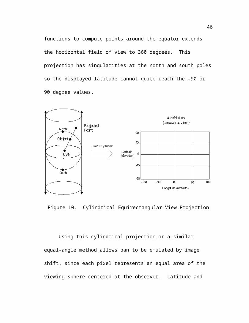
50
If this is the first frame or the camera location changedRender whole framebuffer
ElseIf camera panned, shift image and render new areasGet changed screen area bits from changed voxelsClear all bits for the changed screen areas Render the changed screen areas
Save or display camera framebuffer
Figure 21. Camera Render Pseudocode
The Ray Sample Viewport (RSVP)
The Viewport class implements the RSVP algorithm and contains a
framebuffer, but does not directly perform ray tracing. Pixels from a camera
framebuffer are sampled according to the current viewport transform. This sampling
may cause the camera to trace a requested pixel if it is not current.
Basic 2D transforms [FOLE96] are used to sample pixels from a camera
framebuffer. Any 2D transform may be applied, rotation, scaling and translation are
implemented, while shearing, warping and other effects could be added easily. One
such transform fixes the equal-area projection distortion and restores the standard
view appearance. Methods are defined to set the rotate, scale and translate factors,
which are applied in that order. For each viewport pixel, the camera pixel for the
current set of transforms is sampled, and ray traced if the null color, then copied to
the viewport pixel.

51
Figure 22 shows the pseudocode for the viewport render method that updates
the image using the RSVP algorithm. This also shows how automatic pan and zoom
could be performed if the viewport moves off the camera area, although these features
were not fully implemented (see autopan and autozoom description later in Chapter
VII).
If viewport zoomed beyond camera size range Zoom camera by factor of 2, reuse 1/4 pixels
For each viewport pixelTransform to camera pixel coordinates and sampleIf pixel off edge, pan camera to include pixelIf pixel is erased to null color, ray trace pixelSet pixel color in viewport framebufferSave or display viewport framebuffer
Figure 22. Viewport Render Pseudocode
Lights, Cameras, Action!
The top class, World, contains the entire scene and contains references to
other classes as show in Figure 23. It uses java.util.Vector to maintain lists of lights,
objects, cameras and viewports. This predefined Vector class handles dynamic arrays
and is not the same as the ray tracing Vector3 class that was written to handle
mathematical vectors for ray tracing. Each entity has an animate(frame) method that
is called once per frame to update the entity to its state at the current frame number
time. Methods are provided to add and delete each type of entity. Objects are added
to the appropriate voxels in a uniform spatial subdivision grid and their voxel
locations are updated during animation.

52
World
Grid Light AbstractObject
AbstractCamera
Viewport
Voxel FrameBuffer
FrameBuffer
TemporalBitmap
Light AbstractObject
AbstractCamera
Viewport
Voxel
Figure 23. World Data Structure
The World animate method is called repeatedly by the user program to render
each frame. Figure 24 shows the pseudocode for this process. It calls the animate
method for each light and object to move them to their location and state for the
current frame. Then each camera is animated to update its pan and zoom state, and
the camera image is rendered. Finally, each viewport is animated to update its
transform state, and the viewport image is rendered by sampling a camera image.
Boolean flags are used to determine what types of changes occurred and perform the
most efficient update. Additional flags allow acceleration options to be turned on and
off for testing.
Animate lights, update changed voxelsAnimate objects, update changed voxelsAnimate cameras, update imagesAnimate viewports, update imagesClear all voxel changed flags
Figure 24. World Animate Pseudocode

53
Table 2 shows the names and descriptions of all the classes developed for this
thesis.
Name DescriptionAbstractCamera View projection and ray tracing accelerationAbstractObject Root of hierarchy for 3D objectsAbstractPlane Unbounded planeBoundedPlane Bounded plane with extentBox Axis-aligned hexahedral parallelopipedCheckerMaterial Checkerboard texture mapColor RGB colorConstants Global constantsCylindricalCamera Cylindrical equirectangular view projection for PanimationExtent Bounding box extentFrameBuffer Image buffer for rendering and TGA filesGrid Uniform spatial subdivisionInteract Interactive virtual reality test programInteractWorld Scene data for virtual reality test programIntersection Data for ray-object intersectionLight Light sourceMaterial Surface color, properties and 3D texture mappingPoint 3D locationPolygon Concave or convex polygon with any number of pointsRay Ray with origin point and direction vectorRayTrace Core ray tracer methodsRing Planar ring with inner and outer radiiShow Program to view a TGA fileShowMovie Program to animate a set of TGA filesSphere 3D sphereStandardCamera Standard ray tracing view projectionStatistics Maintains counts and timing for resultsTemporalBitmap Temporal coherence animation acceleration bit setTest Test program for resultsVector3 3D vector class, named differently than java.util.VectorViewport Ray Sample Viewport (RSVP)Voxel Uniform spatial subdivision grid cellVoxelIndex Uniform spatial subdivision 3D indexWorld Top class for entire scene
Table 2. Class Names and Descriptions

CHAPTER V
RESULTS
Animation
Several animation programs were written with hard-coded scenes. These
programs loop for several frames, calling the object, camera and viewport animate
methods and writing a TGA file for each frame. These animate methods are designed
to be overriden by user-defined subclasses to allow each entity to change its state for
the current frame. This mechanism is simple and flexible for testing.
The Test program generates a sequence of animation frame TGA files and
provides Boolean flags to control animation and acceleration features. Table 3 shows
results from a 1.1 GHz PC with 256 MB of memory and Java 1.3.1. The sequences
are 1, 10 and 100 frames at 320x200 resolution. The spatial grid is 15x15x10 voxels,
the vertical dimension is smaller. The OSTC method uses 16x16 screen regions with
256 bits in each bitset, the same as Jevans [JEVA92]. The scene contains a
checkerboard ground plane, 12 polygons, 19 spheres and 2 light sources. A
cylindrical camera is used with field of view 100 degrees.
The table shows that panning 3.6 degrees per frame was accelerated using
Panimation by about a factor of 10. Zooming by a 2:1 ratio was accelerated using
RSVP by about a factor of 10. Animation of a small bouncing ball in this scene was
accelerated using OSTC by about a factor of 2. Simultaneous pan, zoom and

55
animation caused complex view changes and was accelerated by about a factor of 2.
Unlike most earlier approaches, these techniques can be used to accelerate pan, zoom
and animation simultaneously. The resulting 100 frame animation sequences were
converted to animated GIF files and are available for review. These results are very
encouraging and indicate that even greater performance can be achieved for slower
pan and zoom or longer animation sequences.
Traditional Algorithm Accelerated AlgorithmType of Operation
Number of Frames
Number of Rays
Execution Time (sec)
Number of Rays
Execution Time (sec)
Pan 1 64000 1.2 64000 1.110 640000 9.4 83800 1.7100 6400000 69.6 281800 6.9
Zoom 1 64000 1.3 63922 1.810 640000 12.1 154616 4.4100 6400000 120.8 165957 18.9
Animate 1 64000 1.1 64000 1.510 640000 9.8 222160 5.8100 6400000 96.2 1633360 43.6
Pan, Zoom and Animate
1 64000 1.3 63922 2.010 640000 11.5 221384 6.4100 6400000 71.3 880475 31.8
Table 3. Acceleration Results
Figure 25 shows a test image where the black areas are rectangles erased to
the null color by pan and object animation. The narrow black strips at the top and
right are caused by the camera panning slightly up and right, shifting the image down
and left. The irregular black area at the bottom center of the image is caused by
OSTC screen areas invalidated by a small moving object in that area. Only the black

56
areas need to be ray traced, the majority of the image is reused from the previous
frame, showing the potential for image space acceleration even with simultaneous pan
and object animation. The field of view angle is wider than usual at 100 degrees and
shows the cylindrical distortion of the square checkerboard.
Figure 25. Simultaneous Pan and Animation Image
Figure 26 shows a camera image and two smaller viewport images extracted
from the camera image. In the camera image, only the pixels sampled by the
viewports were ray traced, the black areas are null pixels not traced. This
demonstrates how a large camera buffer traces rays as needed, with many pixels
shared between the two viewports and traced only once. The rotated viewport

57
illustrates how scattered pixels may be sampled and has one corner slightly off the
camera image. This missing corner shows a case where autopan could have panned
the camera slightly and prevented the image defect.
a.) 640x480 camera image with sampled pixels
b.) 320x200 sampled zoom viewport c.) 320x200 zoom and rotate viewport
Figure 26. Camera and Viewport Images

58
Virtual reality
An interactive test program was written to provide virtual reality style
interaction. Figure 27 shows the interactive test program windows, with a camera
image and control buttons on the left and a viewport image and buttons on the right.
Buttons are provided to control panning, zooming and other effects, to control
acceleration options and to select a standard or cylindrical projection for the viewport.
The viewport in the figure is set to standard to correct the cylindrical distortion and
has been zoomed to show the hourglass shape resulting from sampling a rectangular
cylindrical image. Normally, the viewport would not be zoomed this way and would
have a complete image with no black edge, similar to Figure 16.
In addition to the square checkerboard ground plane shown, a checkerboard-
textured circular disk was also tested, providing a flat horizon with the cylindrical
projection. The camera supports accelerated pan using the Panimation algorithm,
while the viewport provides accelerated pan, zoom and rotate using the RSVP
algorithm. The user can move the viewpoint through the scene, although the entire
image must be ray traced. The resulting interaction is similar to virtual reality and
panoramic image systems, allowing the user to scan around the scene and zoom in on
details. Unlike panoramic bitmapped images, zooming with this method shows exact
detail using ray tracing. The viewport allows very fast pan, zoom and rotate on the
camera image using the RSVP algorithm with little or no additional ray tracing. This
program demonstrates the major features of the algorithms presented in this thesis.
The interaction program is valuable for testing, provides good demonstrations and is
fun to use.

59
Figure 27. Interactive Camera and Viewport Windows

CHAPTER VII
FUTURE WORK
This thesis has focused on acceleration, but many other features could be
added. Realism could be improved by interpolating sampled pixel colors,
antialiasing, distribution ray tracing and improved texture mapping. Not all the
possible features mentioned earlier are fully implemented. Although these
acceleration techniques are intended for ray tracing, some of them could be applied to
other rendering methods, such as z-buffer or scan-line.
Autopan and Autozoom
When a viewport hits a buffer edge or size limit, it can trigger an autopan
(automatic pan) or autozoom (automatic zoom) event, as shown in Figure 28.
Autozoom could double or halve the buffer scale and reuse ¼ of the pixels as
described earlier. Careful alignment of primary rays or supersampling can reduce
visible “popping” when the scale is changed by a factor of two.
Ray Traced Camera Frame Buffer
Viewports
Viewporttoo smallor largecan causeautozoom
Viewportoff edgecan causeautopan
Figure 28. Viewport Autopan and Autozoom

61
Autopan could use many different strategies, such as moving the minimum or
maximum amount, recentering the viewport or moving the four viewport corners onto
the buffer. The application could set the general strategy for each scene, for example,
if a large pan is planned, the autopan scroll amount could be the maximum amount.
If one viewport causes a pan or zoom, any other viewports must account for the
camera change. Multiple viewports complicate autopan and autozoom, perhaps not
all viewports should be allowed this capability.
Autopan or autozoom could cause “thrashing,” similar to operating system
paging problems. Thrashing may occur if a viewport or set of viewports continues to
sample pixels off the frame buffer, causing the camera to be automatically panned or
zoomed back and forth inefficiently. This can be reduced by zooming out to the
largest field of view for the current viewports, allocating a larger frame buffer, and
other techniques. The order that multiple viewports on the same buffer are processed
could also be ordered to process nearby viewports together for more coherence.
The screen x,y order of ray tracing pixels does not matter much for the camera
or ray tracing in general, but a localized pixel rendering order for the viewports can
reduce thrashing. To avoid repeated buffer panning back and forth, the viewport
pixel scan order could be localized rather than sweeping across the whole area for
each scan line. The viewport area could be divided into a checkerboard grid with
each grid square traversed separately. Perhaps another pixel traversal method like the
quadtree algorithm might be effective.
To avoid thrashing with warped viewports, such as the inverse cylindrical
mapping, a set of smaller buffers could be allocated instead of a single large buffer.

62
The arrangement of allocated buffer blocks would adapt to any well-behaved
sampling pattern, reducing memory usage and thrashing. A least recently used (LRU)
or similar scheme could be used to select blocks for reuse.
By requesting that pixels be ray traced as needed, and automatically panning
or zooming the parent camera, the viewport does much more than simple image
postprocessing. It is a dynamic part of the ray tracing that controls the camera during
the animation and acts as an extended camera at a higher level of abstraction.
View projections
Other view projections that give equal area per pixel could be used instead of
the cylindrical equirectangular projection. The simple orthographic projection with
parallel rays has no depth perspective but is useful in fields such as CAD and data
visualization. Fisheye projections [GLAE99] map equal angles from the center of
view to concentric circles, giving a circular panorama image instead of rectangular.
The radial symmetry of fisheye projections might not be suited to rectangular pixels
though. Bourgoin [BOUR99] describes a “bowlic” projection that maps the image
area to a sphere surrounding the scene with view rays pointing to the sphere center.
This gives an unusual perspective that shows the scene from every direction
simultaneously, outside-in instead of the usual inside-out spherical projection.
Command language
An input scene definition file format could be defined for ease of use. Java
code proved adequate and flexible for hard-coded initial test cases, but text command
files might be preferred by some people, especially non-programmers. However,

63
these formats tend to limit flexibility unless full expression parsing and control
structures are provided, in effect creating a new programming language and returning
to the same situation. Many useful techniques, such as object-oriented inheritance
and polymorphism, would be difficult to implement in a command language.
Interaction
The interactive test program could be enhanced for virtual reality, interactive
scene editing and other applications. It could easily be changed to an applet running
in a web page. Progressive rendering [GHAN99] can be used to accelerate an
interactive application by first ray tracing and displaying a low resolution image, then
tracing and displaying the in-between pixels in increasing detail. This provides a
quick preview of the whole image while rendering continues. The scheme could
work well with the 2:1 zoom technique mentioned before, reusing ¼ of the previous
pixels.
Compression
Data compression could be added by saving the shift offset and redrawn
rectangles for each frame instead of the whole image. This is a form of delta
compression, where only the differences between frames are saved. The entire first
frame image could be written to a file, followed by shift commands and retraced
blocks for each successive frame. The decoder program can load the first frame and
play back the differences, reusing previous frame data the same as the acceleration
scheme does. Yoon [YOON00] combined ray tracing and data compression in a
similar way using reprojection. The Motion Picture Experts Group (MPEG) video

64
format performs compression similarly using differences between frames and motion
compensation for moving objects [GHAN99].
Postprocessing
A program could be written to read and average a set of TGA files into a
single TGA file. Antialiasing and distribution ray tracing could then be performed by
jittering rays differently in each frame. The final average image could have motion
blur, depth of field and other blur effects. This could be extended to a sliding window
that averages small sets of adjacent frames over an entire animation.
Testing
A more rigorous test suite could be used to check performance. Haines
[HAIN87] produced the Standard Procedural Database (SPD) test cases for ray traced
still images. He defined a simple Neutral File Format (NFF) for the scenes. The test
cases are fairly simple and not too typical of real scenes, containing hundreds of
objects to test acceleration schemes. Lext [LEXT01] extended this idea to a
Benchmark for Animated Ray Tracing (BART), a set of three animation scenes. The
scenes are complex and large to stress animation systems and are fairly typical of
modern animation cases.
Cached image blocks
Instead of the Panimation camera image buffer, viewports could sample
smaller blocks of pixels that are dynamically allocated as needed. This could
eliminate any duplicate pixels across cameras and adapt to warped viewport sampling

65
patterns. It could also simplify processing of OSTC bits by avoiding wrapping.
Zoom presents the problem of blocks at different resolutions, which could be handled
as a quadtree for greater pixel reuse. Hierarchical multiresolution encoding could be
used for efficiency with a range of resolutions [GHAN99].
Spatial subdivision
Other spatial subdivision methods could be tried, including adaptive, octree
and BSP tree [GLAS89]. A camera-centered view frustrum grid [MOLL99] as
shown in Figure 29 could provide some advantages. This aligns 2D image space and
3D object space nicely, the voxel grid projects to a 2D grid similar to the OSTC
screen areas. Primary ray traversal is simplified to incrementing an index along one
axis of the voxel array. Distant voxels are larger, providing a better object
distribution and combining advantages of uniform and non uniform grids. However,
initialization and secondary ray traversal are somewhat more complicated, and the
grid is view dependent.
Figure 29. View Frustrum Grid
Eye
View Frustrum Grid

66
Generalized acceleration
Saved ray trees [BRIE96] or saved shading parameters [SEQU89] could be
used for faster image update after light source changes. This would be especially
useful for interactive scene editing, allowing light color and location changes, and
object color and texture changes with very fast response time. The OSTC method can
accelerate light changes, but not as efficiently.
Reprojection [ADEL95] could be used to accelerate camera location changes,
which is the one animation category not accelerated by the techniques in this thesis.
This technique exploits another form of view coherence and works effectively for
small changes. The OSTC bits would probably have to be cleared to start over, since
all rays will differ.
A combination of the techniques in this thesis with reprojection (and possibly
saved ray trees and/or saved shading parameters) would be able to accelerate all types
of animation change. This suggests that it may be possible to develop a standard
animation acceleration approach that unifies earlier separate algorithms in the same
way that Whitted [WHIT80] defined the standard ray tracing algorithm. This would
be a major advance, but there may not be a universal acceleration solution for many
years.
CHAPTER VI
CONCLUSION
This thesis has presented the history and theory of ray tracing and animation
acceleration. The static camera limitation of Jevans [JEVA92] and other earlier work
was noted and the lack of an image space view acceleration algorithm was identified.
New image space algorithms were developed to accelerate pan, zoom and other
effects from a fixed viewpoint. Fast pan is performed using image shifting with an
equal-angle view projection. Fast zoom and other effects are performed using a
sampling viewport and 2D transforms.
A Java ray tracer was implemented to test the new algorithms both for
animation and interaction. An object space temporal coherence animation
acceleration method based on the Jevans [JEVA92] technique was also implemented
and integrated with the new algorithms. The resulting system supports ray traced
animation with acceleration for both object changes and camera field of view
changes. A generalized animation methodology was developed that could be
extended to include reprojection, saved ray trees and other accelerations.
The timing results show performance gains of an order of magnitude for the
new pan and zoom algorithms. This work has been successful, personally rewarding,
and has many applications and possibilities for future work. Possible uses include
animation, interactive scene editing, virtual reality, video games, simulations,
computer-aided design and 3D data visualization.

BIBLIOGRAPHY
[ADEL95] Adelson, S., Hodges, L., “Generating Exact Ray Traced Animation
Frames by Reprojection,” IEEE CG&A, May 1995, pp. 43-52
[AMAN87] Amantides, J., “Realism in Computer Graphics,” IEEE Computer
Graphics & Applications, January 1987, pp.44-56
[AMAN87] Amantides, J., Woo, A., “A Fast Voxel Traversal Algorithm for Ray
Tracing,” Proceedings of Eurographics, 1987, pp. 3-10
[APPE68] Appel, A., “Some Techniques for Shading Machine Renderings of
Solids,” Proceedings of AFIPS JSCC, 1968, Vol. 32, pp. 37-45
[ARNO98] Arnold, K., Gosling, J., The Java Programming Language, Addison-
Wesley, 1998
[ARVO86] Arvo, J., “Backward Ray Tracing,” SIGGRAPH 86 Developments in Ray
Tracing Course Notes, Vol. 12, August 1986
[ARVO87] Arvo, J., Kirk, D., “Fast Ray Tracing by Ray Classification,” Computer
Graphics, July 1987, Vol. 21, No. 4, pp. 55-64
[BOUR99] Bourgoin, V., Farenc, N., Roelens, M., “Creating Special Effects by Ray-
Tracing with Non Classical Perspectives,” ligwww.epfl.ch/~nathalie, 1999
[BRIE96] Briere, N., Poulin, P., “Hierarchical View-dependent Structures for
Interactive Scene Manipulation,” Computer Graphics Proceedings, 1996,
pp. 83-90
69
[CHAP90] Chapman, J., Calvert, T., “Exploiting Temporal Coherence in Ray
Tracing,” Proceedings of Graphics Interface 90, 1990, pp. 196-204
[CLEA88] Cleary, J., Wyvill, G., “Analysis of an Algorithm for Fast Ray Tracing
Using Uniform Space Subdivision,” The Visual Computer, July 1988,
Vol. 4, pp. 65-83
[COOK84] Cook, R., Porter, T., Carpenter, L., “Distributed Ray Tracing,” Computer
Graphics, July 1984, Vol. 18, No. 3, pp. 137-144
[EBER01] Eberly, D., 3D Game Engine Design, Morgan Kaufmann Publishers, 2001
[FOLE96] Foley, J., Van Dam, A., Feiner, S., Hughes, J., Computer Graphics
Principles and Practice, Addison-Wesley, 1996
[FUJI86] Fujimoto, A., Tanaka, T., Iwata, K., “ARTS: Accelerated Ray Tracing
System,” IEEE Computer Graphics & Applications, Apr 1986, pp. 16-26
[GHAN99] Ghanbari, M., Video Coding, The Institution of Electrical Engineers, 1999
[GLAE99] Glaeser, G., Groller, E., “Fast Generation of Curved Perspectives for
Ultra-Wide-Angle Lenses in VR Applications,” The Visual Computer,
July 1999
[GLAS84] Glassner, A., “Space Subdivision for Fast Ray Tracing,” IEEE Computer
Graphics & Applications, Oct 1984, Vol. 4, No. 10, pp. 15-22
[GLAS88] Glassner, A., “Spacetime Ray Tracing for Animation,” IEEE Computer
Graphics & Applications, March 1988, Vol. 8, No. 2, pp. 60-70
[GLAS89] Glassner, A., An Introduction to Ray Tracing, Academic Press, 1989
[HAIN87] Haines, E., “A Proposal for Standard Graphic Environments IEEE
Computer Graphics & Applications, Nov 1987, Vol. 7, No. 11, pp. 3-5

70
[JENS01] Jensen, H., Realistic Image Synthesis Using Photon Mapping, A. K. Peters,
2001
[JEVA89] Jevans, D., “Adaptive Voxel Subdivision for Ray Tracing,” Proceedings of
Graphics Interface 89, 1989, pp. 164-172
[JEVA92] Jevans, D., “Object Space Temporal Coherence for Ray Tracing,”
Proceedings of Graphics Interface 92, May 1992, pp. 176-183
[LEXT01] Lext, J., Assarsson, U., Moller, T., “BART: A Benchmark for Animated
Ray Tracing,” IEEE Computer Graphics & Applications, March 2001,
Vol. 21, No. 2, pp. 22-31
[LOGA89] Logan, J., “The Modified Slicing Extent Technique for Space Subdivision
While Ray Tracing,“ MS thesis, University of Colorado at Colorado
Springs, 1989
[MOLL99] Moller, T., Haines, E., Real-Time Rendering, A K Peters, Ltd, 1999
[MURA90] Murakami, K., Hirota, K., “Incremental Ray Tracing,” Proceedings of
Eurographics Workshop on Photosimulation, June 1990, pp. 15-29
[MUSG92] Musgrave, K., “A Panoramic Virtual Screen for Ray Tracing,” Graphic
Gems III, Academic Press, 1992, pp. 288-294
[OROU98] O’Rourke, M., Principles of Three-Dimensional Computer Animation,
WW Norton & Co, 1998
[PAET90] Paeth, A., “Digital Cartography for Computer Graphics,” Graphic Gems,
Academic Press, 1990, pp. 307-325
[PARK99] Parker, S., et al, “Interactive Ray Tracing,” Symposium on Interactive 3D
Computer Graphics, Apr 1999

71
[PHAR97] Pharr, M., et al, “Rendering Complex Scenes with Memory Coherent Ray
Tracing,” Proceedings of SIGGRAPH 97, 1997
[REIN00] Reinhard, E., Smits, B., Hansen, C., “Dynamic Acceleration Structures for
Interactive Ray Tracing,” Proceedings of Eurographics Workshop on
Rendering, June 2000
[SEMW87] Semwal, S., “The Slicing Extent Technique for Fast Ray Tracing,“ PhD
dissertation, University of Central Florida, Orlando, 1987
[SEQU89] Sequin, C., Smyrl, E., “Parameterized Ray Tracing, “Computer Graphics,
July 1989, Vol. 23, No. 3, pp. 307-314
[SHIR00] Shirley, P., Realistic Ray Tracing, A K Peters, Ltd, 2000
[WALD01] Wald, I., Slusallek, P., Benthin, C., Wagner, M., “Interactive Rendering
with Coherent Ray Tracing,” Proceedings of Eurographics, 2001
[WATT92] Watt, A., Watt, M., Advanced Animation and Rendering Techniques,
Addison-Wesley, 1992
[WHIT80] Whitted, T., “An Improved Illumination Model for Shaded Display,”
Communications of the ACM, June 1980, Vol. 23, No. 6, pp. 343-349
[YOON00] Yoon, T., Neumann, U., “IBRAC: Image-Based Rendering Acceleration
and Compression,” http://graphics.usc.edu/cgit/pdf/papers/hp.pdf

APPENDIX A. PROGRAMMER’S REFERENCE
This is the Read_Me.txt file for the Gage thesis. This code is a Java ray tracer used to study animation acceleration. It was tested with Java 1.3.1 and should be portable.
This code was written by Philip Gage in partial fulfillment of the requirements for the degree of Master of Science, Department of Computer Science. This work was performed at the University of Colorado in Colorado Springs under the direction of Dr S. Semwal from Jan 2000 to May 2002. Refer to the thesis paper "View Coherence Acceleration for Ray Traced Animation " by Philip Gage, 2002, for more information.
Operation
To compile and run the animation test program, enter:javac Test.javajava Test
To compile and run the animation viewer program (with optional delay in integer msec) to display TGA files from Test, enter:
javac ShowMovie.javajava ShowMovie [delay]
To compile and run the image viewer program (with optional filename, default “frame0.tga”) to display a TGA file, enter:
javac Show.javajava Show [filename.tga]
To compile and run the interactive test program, enter:javac Interact.javajava Interact

73
Examples
For coding examples, refer to the Example*.java and Movie*.java program files.The simple Example3.java file is shown below.
public class Example3 {
/** Main program for example */ public static void main (String[] argv) {
// Define and populate scene World world = new World();
// Define a light source world.add(new Light ( new Vector3 (-100.0, -100.0, -50.0), // XYZ direction new Color (1.0, 1.0, 1.0))); // RGB color
// Define a red sphere object on Z axis world.add(new Sphere ( new Point (0.0, 0.0, 500.0), // XYZ center 100.0, // radius new Color (1.0, 0.0, 0.0))); // RGB color
// Define a 320x200 camera, default view (0,0,1) along Z axis world.add (new CylindricalCamera (world, 320, 200));
// Perform ray tracing and write frame0.tga world.animate (); }
}


![Experimental Optics - ASPoptics... · 2021. 1. 17. · coherence area, [2]. Temporal coherence characterizes the ability of a wave to interfere with a copy of itself delayed by a](https://img.pdfslide.us/doc/110x75/60bf93c5f1310212c775167d/experimental-optics-asp-optics-2021-1-17-coherence-area-2-temporal.jpg)