Vibrations of Single Degree of Freedom Systemslibvolume3.xyz/.../forcedvibrationsofsingledegreefreedo… · · 2014-05-28Vibrations of Single Degree of Freedom Systems CEE 541

Vibrations of Single Degree of Freedom SystemsCEE 541. Structural Dynamics

Department of Civil and Environmental EngineeringDuke University

Henri P. GavinFall, 2014

This document describes the free and forced response of single degree offreedom (SDOF) systems. A single degree of freedom system is a spring-mass-damper system in which the spring has no damping or mass, the mass has nostiffness or damping, the damper has no stiffness or mass. Furthermore, themass is allowed to move in only one direction. The horizontal vibrations of asingle-story building can be conveniently modeled as a single degree of freedomsystem. In part 1 of this document we examine some useful trigonometricidentities. In part 2 of this document we determine how damped SDOFsystems vibrate freely after being released from an initial displacement withsome initial velocity. In part 3 of this document we determine how dampedSDOF systems respond to a persistent sinusoidal forcing.

Consider the structural system shown in Figure 1, where:f(t) = external excitation forcex(t) = displacement of the center of mass of the moving objectm = mass of the moving object, fI = d

dt(mx(t)) = mx(t)c = linear viscous damping coefficient, fD = cx(t)k = linear elastic stiffness coefficient, fS = kx(t)

m

k, c

x(t)f(t)

c

k

x(t)

m f(t)

Figure 1. The proto-typical single degree of freedom oscillator.

2 CEE 541. Structural Dynamics – Duke University – Fall 2014 – H.P. Gavin

The kinetic energy T (x, x), the potential energy, V (x), and the externalforcing and dissipative forces, p(x, x), are

T (x, x) = 12mx(t)2 (1)

V (x) = 12kx(t)2 (2)

p(x, x) = cx(t)− f(t) (3)

The general form of the differential equations describing a SDOF oscillatorfollows directly from Lagrange’s equation,

d

dt

∂T (x, x)∂x

− ∂T (x, x)∂x

+ ∂V (x)∂x

+ p(x, x) = 0 , (4)

or from simply balancing the forces on the mass,∑F = 0 : fI + fD + fS = f(t) . (5)

Either way,

mx(t) + cx(t) + kx(t) = f(t), x(0) = do, x(0) = vo (6)

where the initial displacement is do, and the initial velocity is vo.

The solution to equation (6) is the sum of a homogeneous part (freeresponse) and a particular part (forced response). This document describesfree responses of all types and forced responses to simple-harmonic forcing.

1 Trigonometric and Exponential Forms for Oscillations

We expect the free vibrational response of lightly damped systems todecay over time. Note that damping may be introduced into a structurethrough diverse mechanisms, including linear viscous damping, nonlinear vis-cous damping, visco-elastic damping, friction damping, and plastic deforma-tion. All but linear viscous damping are somewhat complicated to analyzewith closed-form expressions, so we will restrict our attention to linear vis-cous damping, in which the damping force fD is proportional to the velocity,fD = cx.

CC BY-NC-ND H.P. Gavin

http://creativecommons.org/licenses/by-nc-nd/3.0/

Vibrations of Single Degree of Freedom Systems 3

1.1 Constant Amplitude

In general a constant-amplitude oscillation, x(t), of frequency ω can bedescribed by sinusoidal functions. These sinusoidal functions may be equiva-lently written in terms of complex exponentials e±iωt with complex coefficients,X = A + iB and X∗ = A − iB. The complex constant X∗ is the complexconjugate of X.

x(t) = a cos(ωt) + b sin(ωt) (7)= X eiωt +X∗ e−iωt (8)

Proof:

X eiωt +X∗ e−iωt = (A+ iB) (cos(ωt) + i sin(ωt)) +(A− iB) (cos(ωt)− i sin(ωt)) (9)

= A cos(ωt) + iA sin(ωt) + iB cos(ωt)−B sin(ωt) +A cos(ωt)− iA sin(ωt)− iB cos(ωt)−B sin(ωt) (10)

= 2A cos(ωt)− 2B sin(ωt) (11)= a cos(ωt) + b sin(ωt) (12)

Comparing these forms, we see that a = 2A and b = −2B. Note that all ofthe above expressions are exactly equivalent. Equation (7), is exactly the sameas equation (8). Equation (7) is easier to interpret as describing a sinusoidaloscillation, however equation (8) is much easier to work with, mathematically.We will endeavor to use both forms in this document, just to emphasize howthe two forms are one and the same.

Equations (7) and (8) describe a sinusoidal oscillation with a constantamplitude. The amplitude, X, of the oscillation x(t) can be found by addingthe magnitudes of the complex amplitudes X and X∗, or by solving x(t) = 0for t, and substituting into equation (7). Either way, the amplitude of theoscillation is

X = |X|+ |X∗| = 2|X| =√a2 + b2 , (13)




-6

-4

-2

0

2

4

6

0 2 4 6 8 10

response, x(t)

time, t, sec

period, T

am

plit

ude, |X|

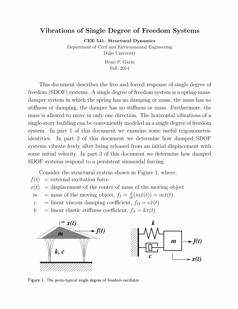
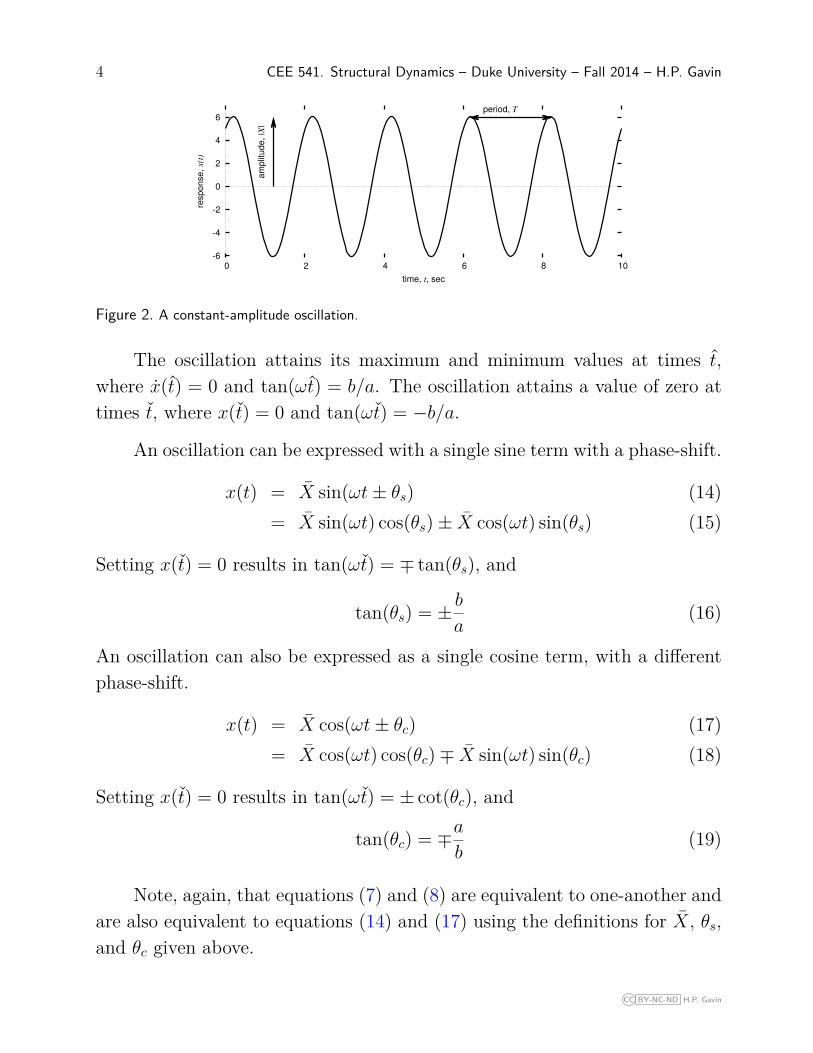
Figure 2. A constant-amplitude oscillation.

The oscillation attains its maximum and minimum values at times t,where x(t) = 0 and tan(ωt) = b/a. The oscillation attains a value of zero attimes t, where x(t) = 0 and tan(ωt) = −b/a.

An oscillation can be expressed with a single sine term with a phase-shift.

x(t) = X sin(ωt± θs) (14)= X sin(ωt) cos(θs)± X cos(ωt) sin(θs) (15)

Setting x(t) = 0 results in tan(ωt) = ∓ tan(θs), and

tan(θs) = ± ba

(16)

An oscillation can also be expressed as a single cosine term, with a differentphase-shift.

x(t) = X cos(ωt± θc) (17)= X cos(ωt) cos(θc)∓ X sin(ωt) sin(θc) (18)

Setting x(t) = 0 results in tan(ωt) = ± cot(θc), and

tan(θc) = ∓ab

(19)

Note, again, that equations (7) and (8) are equivalent to one-another andare also equivalent to equations (14) and (17) using the definitions for X, θs,and θc given above.




1.2 Decaying Amplitude

To describe an oscillation which decays with time, we can multiply theexpression for a constant amplitude oscillation by a positive-valued functionwhich decays with time. Here we will use a real exponential, eσt, where σ < 0.Multiplying equations (7) through (8) by eσt,

x(t) = eσt(a cos(ωt) + b sin(ωt)) (20)= eσt(Xeiωt +X∗e−iωt) (21)= Xe(σ+iω)t +X∗e(σ−iω)t (22)= Xeλt +X∗eλ

∗t (23)

Again, note that all of the above equations are exactly equivalent. The expo-nent λ is complex, λ = σ + iω and λ∗ = σ − iω. If σ is negative, then theseequations describe an oscillation with exponentially decreasing amplitudes.Note that in equation (20) the unknown constants are σ, ω, a, and b. An-gular frequencies, ω, have units of radians per second. Circular frequencies,f = ω/(2π) have units of cycles per second, or Hertz. Periods, T = 2π/ω,have units of seconds.

In the next section we will find that for an un-forced vibration, σ andω are determined from the mass, damping, and stiffness of the system. Wewill see that the constant a equals the initial displacement do, but that theconstant b depends on the initial displacement and velocity, as well mass,damping, and stiffness.

-6

-4

-2

0

2

4

6

0 2 4 6 8 10

response,

x(t

)

time, t, sec

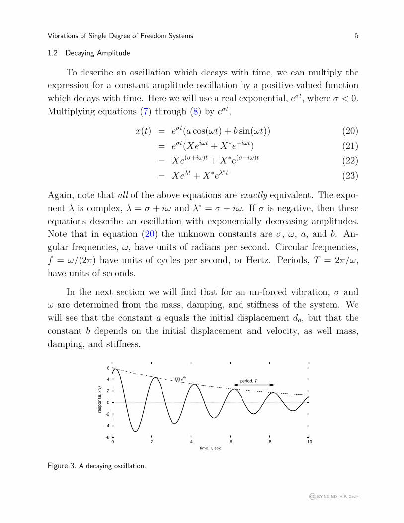
period, T|X| eσt

Figure 3. A decaying oscillation.




2 Free response of systems with mass, stiffness and damping

Using equation (23) to describe the free response of a single degree offreedom system, we will set f(t) = 0 and will substitute x(t) = Xeλt intoequation (6).

mx(t) + cx(t) + kx(t) = 0 , x(0) = do , x(0) = vo , (24)mλ2Xeλt + cλXeλt + kXeλt = 0 , (25)

(mλ2 + cλ+ k)Xeλt = 0 , (26)

Note that m, c, k, λ and X do not depend on time. For equation (26) to betrue for all time,

(mλ2 + cλ+ k)X = 0 . (27)

Equation (27) is trivially satisfied if X = 0. The non-trivial solution is mλ2 +cλ+ k = 0. This is a quadratic equation in λ which has the roots,

λ1,2 = − c

2m ±√√√√( c

2m

)2− k

m. (28)

The solution to a homogeneous second order ordinary differential equationrequires two independent initial conditions: an initial displacement and aninitial velocity. These two independent initial conditions are used to determinethe coefficients, X and X∗ (or A and B, or a and b) of the two linearlyindependent solutions corresponding to λ1 and λ2.

The amount of damping, c, qualitatively affects the quadratic roots, λ1,2,and the free response solutions.

• Case 1 c = 0 “undamped”If the system has no damping, c = 0, and

λ1,2 = ±i√k/m = ±iωn . (29)

This is called the natural frequency of the system. Undamped systemsoscillate freely at their natural frequency, ωn. The solution in this caseis

x(t) = Xeiωnt +X∗e−iωnt = a cosωnt+ b sinωnt , (30)




which is a real-valued function. The amplitudes depend on the initialdisplacement, do, and the initial velocity, vo.

• Case 2 c = cc “critically damped”If (c/(2m))2 = k/m, or, equivalently, if c = 2

√mk, then the discriminant

of equation (28) is zero, This special value of damping is called the criticaldamping rate, cc,

cc = 2√mk . (31)

The ratio of the actual damping rate to the critical damping rate is calledthe damping ratio, ζ.

ζ = c

cc. (32)

The two roots of the quadratic equation are real and are repeated at

λ1 = λ2 = −c/(2m) = −cc/(2m) = −2√mk/(2m) = −ωn , (33)

and the two basic solutions are equal to each other, eλ1t = eλ2t. In orderto admit solutions for arbitrary initial displacements and velocities, thesolution in this case is

x(t) = x1 e−ωnt + x2 t e

−ωnt . (34)

where the real constants x1 and x2 are determined from the initial dis-placement, do, and the initial velocity, vo. Details regarding this specialcase are in the next section.

• Case 3 c > cc “over-damped”If the damping is greater than the critical damping, then the roots, λ1

and λ2 are distinct and real. If the system is over-damped it will notoscillate freely. The solution is

x(t) = x1 eλ1t + x2 e

λ2t , (35)

which can also be expressed using hyperbolic sine and hyperbolic cosinefunctions. The real constants x1 and x2 are determined from the initialdisplacement, do, and the initial velocity, vo.




• Case 4 0 < c < cc “under-damped”If the damping rate is positive, but less than the critical damping rate, thesystem will oscillate freely from some initial displacement and velocity.The roots are complex conjugates, λ1 = λ∗2, and the solution is

x(t) = X eλt +X∗ eλ∗t , (36)

where the complex amplitude depends on the initial displacement, do,and the initial velocity, vo.

We can re-write the dynamic equations of motion using the new dynamicvariables for natural frequency, ωn, and damping ratio, ζ. Note that

c

m= c

√k√k

1√m√m

= c√k√m

√k√m

= 2 c

2√km

√√√√ k

m= 2ζωn. (37)

mx(t) + cx(t) + kx(t) = f(t), (38)

x(t) + c

mx(t) + k

mx(t) = 1

mf(t), (39)

x(t) + 2ζωn x(t) + ω2n x(t) = 1

mf(t), (40)

The expression for the roots λ1,2, can also be written in terms of ωn and ζ.

λ1,2 = − c

2m ±√√√√( c

2m

)2− k

m, (41)

= −ζωn ±√

(ζωn)2 − ω2n , (42)

= −ζωn ± ωn√ζ2 − 1 . (43)

Some useful facts about the roots λ1 and λ2 are:




• λ1 + λ2 = −2ζωn

• λ1 − λ2 = 2 ωn√ζ2 − 1

• ω2n = 1

4(λ1 + λ2)2 − 14(λ1 − λ2)2

• ωn =√λ1λ2

• ζ = −(λ1 + λ2)/(2ωn)

ω

Im

−ω

d

dλ

λ1

2x

x

−ζωn

nω

Re σ = λ

ω = λ

2.1 Free response of critically-damped systems

The solution to a homogeneous second order ordinary differential equa-tion requires two independent initial conditions: an initial displacement andan initial velocity. These two initial conditions are used to determine thecoefficients of the two linearly independent solutions corresponding to λ1 andλ2. If λ1 = λ2, then the solutions eλ1t and eλ2t are not independent. In fact,they are identical. In such a case, a new trial solution can be determined asfollows. Assume a new solution of the form

x(t) = u(t)x1eλ1t , (44)

x(t) = u(t)x1eλ1t + u(t)λ1x1e

λ1t , (45)x(t) = u(t)x1e

λ1t + 2u(t)λ1x1eλ1t + u(t)λ2

1x1eλ1t (46)

substitute these expressions into

x(t) + 2ζωnx(t) + ω2nx(t) = 0 ,

collect terms, and divide by x1eλ1t, to get

u(t) + (2ζωn + 2(−ωn))u(t) = 0

which is a first order ordinary differential equation for u(t). The solution ofthis ordinary differential equation is

u(t) = C ,




from which the new trial solution is found.

u(t) = x2 t

So, using the trial solution x(t) = x1eλt + x2te

λt, and incorporating initialconditions x(0) = do and x(0) = vo, the free response of a critically-dampedsystem is:

x(t) = do e−ωnt + (vo + ωndo) t e−ωnt . (47)

2.2 Free response of underdamped systems

If the system is under-damped, then ζ < 1,√ζ2 − 1 is imaginary, and

λ1,2 = −ζωn ± iωn√|ζ2 − 1| = σ ± iω. (48)

The frequency ωn√|ζ2 − 1| is called the damped natural frequency, ωd,

ωd = ωn√|ζ2 − 1| . (49)

It is the frequency at which under-damped SDOF systems oscillate freely,With these new dynamic variables (ζ, ωn, and ωd) we can re-write the solutionto the damped free response,

x(t) = e−ζωnt(a cosωdt+ b sinωdt), (50)= Xeλt +X∗eλ

∗t. (51)

Now we can solve for X, (or, equivalently, A and B) in terms of the initialconditions. At the initial point in time, t = 0, the position of the mass isx(0) = do and the velocity of the mass is x(0) = vo.

x(0) = do = Xeλ·0 +X∗eλ∗·0 (52)

= X +X∗ (53)= (A+ iB) + (A− iB) = 2A = a. (54)

x(0) = vo = λXeλ·0 + λ∗X∗eλ∗·0, (55)

= λX + λ∗X∗, (56)= (σ + iωd)(A+ iB) + (σ − iωd)(A− iB), (57)= σA+ iωdA+ iσB − ωdB +

σA− iωdA− iσB − ωdB, (58)= 2σA− 2ωB (59)= −ζωn do − 2 ωd B, (60)




from which we can solve for B or b.

B = − vo + ζωndo2ωd

(61)

b = vo + ζωndoωd

(62)

Putting this all together, the free response of an underdamped system to anarbitrary initial condition, x(0) = do, x(0) = vo is

x(t) = e−ζωnt(do cosωdt+ vo + ζωndo

ωdsinωdt

). (63)

-6

-4

-2

0

2

4

6

0 2 4 6 8 10

response,

x(t

)

time, t, sec

damped natural period, Td

|X| e-ζ ω

n t

do

vo

Figure 4. Free response of an under-damped oscillator to an initial displacement and velocity.

2.3 Free response of over-damped systems

If the system is over-damped, then ζ > 1, and√ζ2 − 1 is real, and the

roots are both real and negative

λ1,2 = −ζωn ± ωn√ζ2 − 1 = σ ± ωd. (64)

Substituting the initial conditions x(0) = do and x(0) = vo into thesolution (equation (35)), and solving for the coefficients results in

x1 = vo + do(ζωn + ωd)2ωd

, (65)

x2 = do − x1 . (66)




Substituting the hyperbolic sine and hyperbolic cosine expressions for theexponentials results in

x(t) = e−ζωnt(do coshωdt+ vo + ζωndo

ωdsinhωdt

). (67)

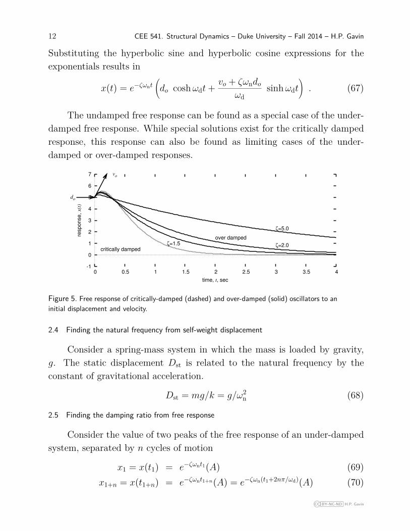
The undamped free response can be found as a special case of the under-damped free response. While special solutions exist for the critically dampedresponse, this response can also be found as limiting cases of the under-damped or over-damped responses.

-1

0

1

2

3

4

5

6

7

0 0.5 1 1.5 2 2.5 3 3.5 4

response, x(t)

time, t, sec

do

vo

critically damped

over dampedζ=1.5 ζ=2.0

ζ=5.0

Figure 5. Free response of critically-damped (dashed) and over-damped (solid) oscillators to aninitial displacement and velocity.

2.4 Finding the natural frequency from self-weight displacement

Consider a spring-mass system in which the mass is loaded by gravity,g. The static displacement Dst is related to the natural frequency by theconstant of gravitational acceleration.

Dst = mg/k = g/ω2n (68)

2.5 Finding the damping ratio from free response

Consider the value of two peaks of the free response of an under-dampedsystem, separated by n cycles of motion

x1 = x(t1) = e−ζωnt1(A) (69)x1+n = x(t1+n) = e−ζωnt1+n(A) = e−ζωn(t1+2nπ/ωd)(A) (70)




The ratio of these amplitudes is

x1

x1+n= e−ζωnt1

e−ζωn(t1+2nπ/ωd) = e−ζωnt1

e−ζωnt1e−2nπζωn/ωd= e2nπζ/

√1−ζ2

, (71)

which is independent of ωn and ωd. Defining the log decrement δ(ζ) asln(x1/x1+n)/n,

δ(ζ) = 2πζ√1− ζ2 (72)

and, inversely,ζ(δ) = δ√

4π2 + δ2 ≈δ

2π (73)

where the approximation is accurate to within 3% for ζ < 0.2 and is accurateto within 1.5% for ζ < 0.1.

2.6 Summary

To review, some of the important expressions relating to the free responseof a single degree of freedom oscillator are:

mx(t) + cx(t) + kx(t) = 0 , x(0) = do, x(0) = vo

x(t) + 2ζωnx(t) + ω2nx(t) = 0 , x(0) = do, x(0) = vo

ωn =√√√√ k

m

ζ = c

cc= c

2√mk

ωd = ωn√|ζ2 − 1|

δ = 1n

ln(x1

x1+n

)

ζ(δ) = δ√4π2 + δ2 ≈

δ

2π




3 Response of systems with mass, stiffness, and damping to sinusoidal forcing

When subject to simple harmonic forcing with a forcing frequency ω,dynamic systems initially respond with a combination of a transient responseat a frequency ωd and a steady-state response at a frequency ω. The transientresponse at frequency ωd decays with time, leaving the steady state responseat a frequency equal to the forcing frequency, ω. This section examines threeways of applying forcing: forcing applied directly to the mass, inertial forcingapplied through motion of the base, and forcing from a rotating eccentricmass.

3.1 Direct Force Excitation

If the SDOF system is dynamically forced with a sinusoidal forcing func-tion, then f(t) = F cos(ωt), where ω is the frequency of the forcing, in radiansper second. If f(t) is persistent, then after several cycles the system will re-spond only at the frequency of the external forcing, ω. Let’s suppose thatthis steady-state response is described by the function

x(t) = a cosωt+ b sinωt, (74)

thenx(t) = ω(−a sinωt+ b cosωt), (75)

andx(t) = ω2(−a cosωt− b sinωt). (76)

Substituting this trial solution into equation (6), we obtain

mω2 (−a cosωt− b sinωt) +cω (−a sinωt+ b cosωt) +k (a cosωt+ b sinωt) = F cosωt. (77)

Equating the sine terms and the cosine terms

(−mω2a+ cωb+ ka) cosωt = F cosωt (78)(−mω2b− cωa+ kb) sinωt = 0, (79)




which is a set of two equations for the two unknown constants, a and b, k −mω2 cω

−cω k −mω2

ab

= F

0

, (80)

for which the solution is

a(ω) = cω

(k −mω2)2 + (cω)2 F (81)

b(ω) = k −mω2

(k −mω2)2 + (cω)2 F . (82)

The forced vibration solution (equation (74)) may be written

x(t) = a(ω) cosωt+ b(ω) sinωt = X(ω) cos(ωt+ θc). (83)

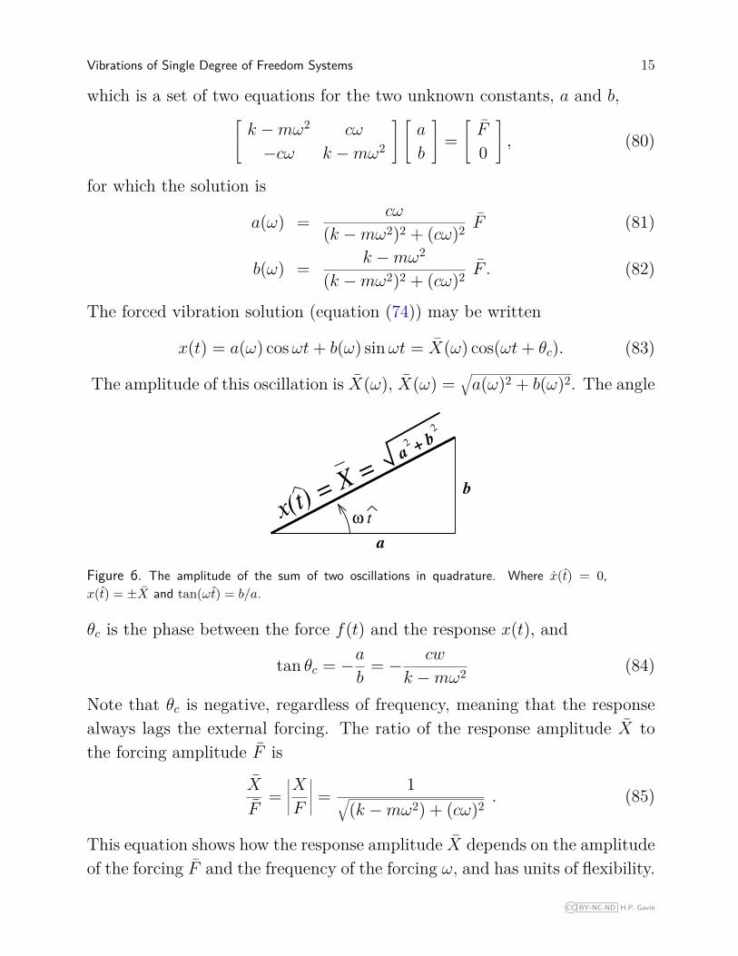
The amplitude of this oscillation is X(ω), X(ω) =√a(ω)2 + b(ω)2. The angle

ω tx(t) = X =

a + b

2

2

a

b

Figure 6. The amplitude of the sum of two oscillations in quadrature. Where x(t) = 0,x(t) = ±X and tan(ωt) = b/a.

θc is the phase between the force f(t) and the response x(t), and

tan θc = −ab

= − cw

k −mω2 (84)

Note that θc is negative, regardless of frequency, meaning that the responsealways lags the external forcing. The ratio of the response amplitude X tothe forcing amplitude F is

X

F=∣∣∣∣∣XF

∣∣∣∣∣ = 1√(k −mω2) + (cω)2

. (85)

This equation shows how the response amplitude X depends on the amplitudeof the forcing F and the frequency of the forcing ω, and has units of flexibility.




Let’s re-derive this expression using complex exponential notation! Theequations of motion are

mx(t) + cx(t) + kx(t) = F cosωt = Feiωt + Fe−iωt . (86)

In a solution of the form, x(t) = Xeiωt + X∗e−iωt, the coefficient X corre-sponds to the positive exponents (positive frequencies), and X∗ correspondsto negative exponents (negative frequencies). Positive exponent coefficientsand negative exponent coefficients are independent and may be found sepa-rately. Considering the positive exponent solution, the forcing is expressed asFeiωt and the partial solution Xeiωt is substituted into the forced equationsof motion, resulting in

(−mω2 + ciω + k) X eiωt = F eiωt , (87)

from whichX

F= 1

(k −mω2) + i(cω) , (88)

which is complex-valued. This complex function has a magnitude∣∣∣∣∣XF∣∣∣∣∣ = 1√

(k −mω2)2 + (cω)2, (89)

the same as equation (85) but derived using eiωt in just three simple lines.

Equation (88) may be written in terms of the dynamic variables, ωn andζ. Dividing the numerator and the denominator of equation (85) by k, andnoting that F/k is a static displacement, xst, we obtain

X

F= 1/k(

1− mk ω

2)

+ i(ckω

) , (90)

X = F/k(1−

(ωωn

)2)+ i

(2ζ ω

ωn

) , (91)

X

xst= 1

(1− Ω2) + i (2ζΩ) , (92)

X

xst= 1√

(1− Ω2)2 + (2ζΩ)2 , (93)




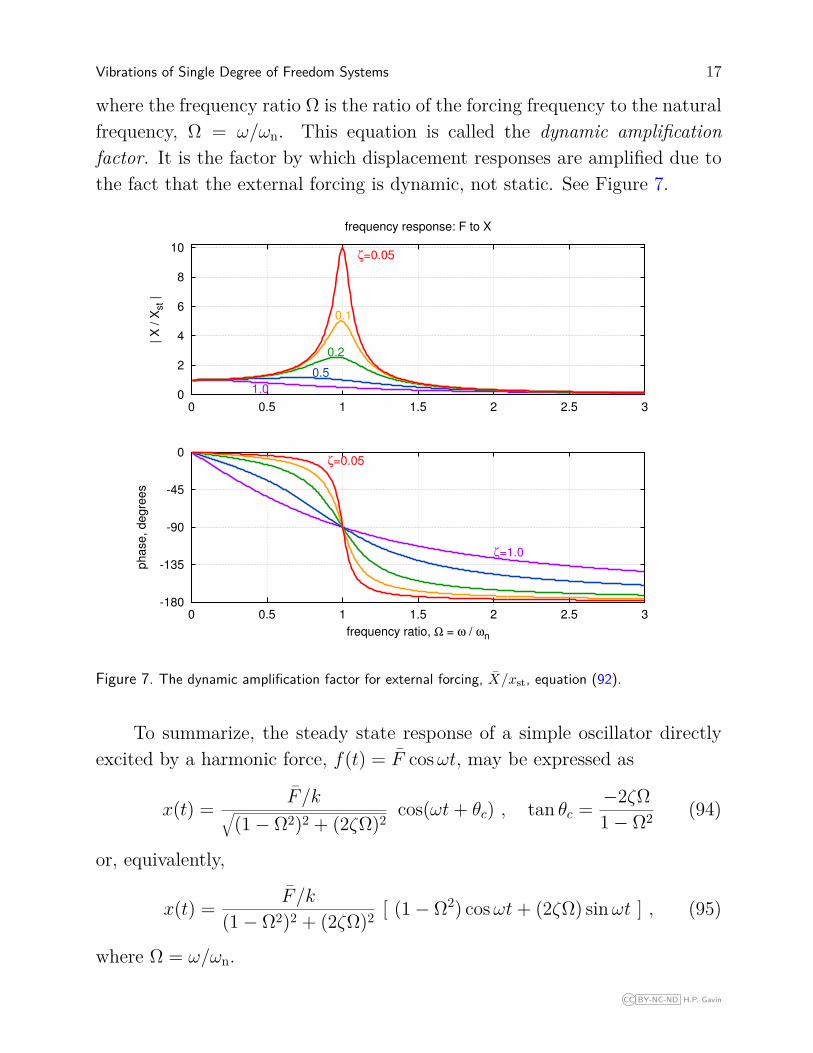
where the frequency ratio Ω is the ratio of the forcing frequency to the naturalfrequency, Ω = ω/ωn. This equation is called the dynamic amplificationfactor. It is the factor by which displacement responses are amplified due tothe fact that the external forcing is dynamic, not static. See Figure 7.

-180

-135

-90

-45

0

0 0.5 1 1.5 2 2.5 3

ph

ase

, d

eg

ree

s

frequency ratio, Ω = ω / ωn

ζ=0.05

ζ=1.0

0

2

4

6

8

10

0 0.5 1 1.5 2 2.5 3

| X

/ X

st |

frequency response: F to X

ζ=0.05

0.1

0.2

0.5

1.0

Figure 7. The dynamic amplification factor for external forcing, X/xst, equation (92).

To summarize, the steady state response of a simple oscillator directlyexcited by a harmonic force, f(t) = F cosωt, may be expressed as

x(t) = F /k√(1− Ω2)2 + (2ζΩ)2

cos(ωt+ θc) , tan θc = −2ζΩ1− Ω2 (94)

or, equivalently,

x(t) = F /k

(1− Ω2)2 + (2ζΩ)2 [ (1− Ω2) cosωt+ (2ζΩ) sinωt ] , (95)

where Ω = ω/ωn.




3.2 Support Acceleration Excitation

When the dynamic loads are caused by motion of the supports (or theground, as in an earthquake) the forcing on the structure is the inertial forceresisting the ground acceleration, which equals the mass of the structure timesthe ground acceleration, f(t) = −mz(t).

m

k, cc

k

m

x(t)

z(t) z(t) x(t)

Figure 8. The proto-typical SDOF oscillator subjected to base motions, z(t)

m ( x(t) + z(t) ) + cx(t) + kx(t) = 0 (96)mx(t) + cx(t) + kx(t) = −mz(t) (97)

x(t) + 2ζωnx(t) + ω2nx(t) = −z(t) (98)

Note that equation (98) is independent of mass. Systems of different massesbut with the same natural frequency and damping ratio have the same be-havior and respond in exactly the same way to the same support motion.

If the ground displacements are sinusoidal z(t) = Z cosωt, then theground accelerations are z(t) = −Zω2 cosωt, and f(t) = mZω2 cosωt. Usingthe complex exponential formulation, we can find the steady state responseas a function of the frequency of the ground motion, ω.

mx(t) + cx(t) + kx(t) = mZω2 cosωt = mZω2eiωt +mZω2e−iωt (99)

The steady-state response can be expressed as the sum of independent com-plex exponentials, x(t) = Xeiωt + X∗e−iωt. The positive exponent parts areindependent of the negative exponent parts and can be analyzed separately.




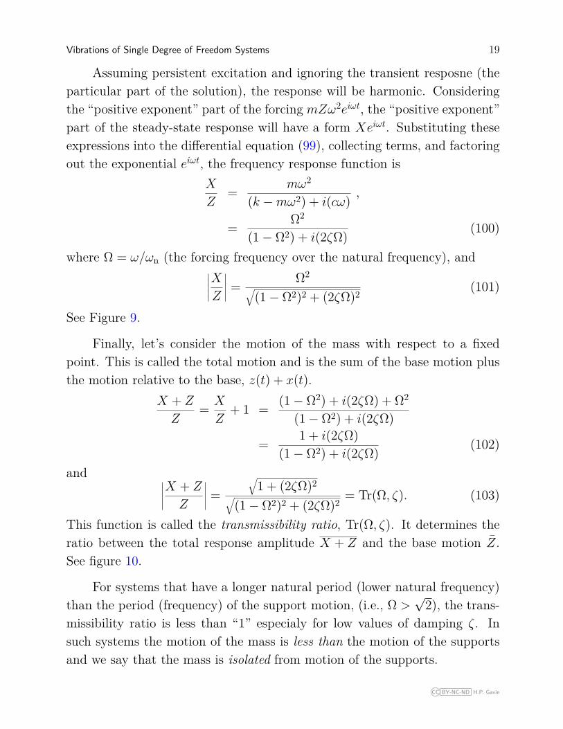
Assuming persistent excitation and ignoring the transient resposne (theparticular part of the solution), the response will be harmonic. Consideringthe “positive exponent” part of the forcing mZω2eiωt, the “positive exponent”part of the steady-state response will have a form Xeiωt. Substituting theseexpressions into the differential equation (99), collecting terms, and factoringout the exponential eiωt, the frequency response function is

X

Z= mω2

(k −mω2) + i(cω) ,

= Ω2

(1− Ω2) + i(2ζΩ) (100)

where Ω = ω/ωn (the forcing frequency over the natural frequency), and∣∣∣∣∣XZ∣∣∣∣∣ = Ω2√

(1− Ω2)2 + (2ζΩ)2(101)

See Figure 9.

Finally, let’s consider the motion of the mass with respect to a fixedpoint. This is called the total motion and is the sum of the base motion plusthe motion relative to the base, z(t) + x(t).

X + Z

Z= X

Z+ 1 = (1− Ω2) + i(2ζΩ) + Ω2

(1− Ω2) + i(2ζΩ)

= 1 + i(2ζΩ)(1− Ω2) + i(2ζΩ) (102)

and ∣∣∣∣∣X + Z

Z

∣∣∣∣∣ =√

1 + (2ζΩ)2√(1− Ω2)2 + (2ζΩ)2

= Tr(Ω, ζ). (103)

This function is called the transmissibility ratio, Tr(Ω, ζ). It determines theratio between the total response amplitude X + Z and the base motion Z.See figure 10.

For systems that have a longer natural period (lower natural frequency)than the period (frequency) of the support motion, (i.e., Ω >

√2), the trans-

missibility ratio is less than “1” especialy for low values of damping ζ. Insuch systems the motion of the mass is less than the motion of the supportsand we say that the mass is isolated from motion of the supports.




-180

-135

-90

-45

0

0 0.5 1 1.5 2 2.5 3

ph

ase

, d

eg

ree

s


ζ=0.05

ζ=1.0

0

2

4

6

8

10

0 0.5 1 1.5 2 2.5 3

| X /

Z |

frequency response: Z to X

ζ=0.05

0.1

0.2

0.5

1.0

Figure 9. The dynamic amplification factor for base-excitation, X/Z, equation (100).

-180

-135

-90

-45

0

0 0.5 1 1.5 2 2.5 3

ph

ase

, d

eg

ree

s


ζ=0.05

ζ=1.0

0

2

4

6

8

10

0 0.5 1 1.5 2 2.5 3

| (X

+Z

) /

Z |

transmissibility: Z to (X+Z)

ζ=0.05

0.1

0.2

0.5ζ=1.0

Figure 10. The transmissibility ratio |(X + Z)/Z| = Tr(Ω, ζ), equation (102).




3.3 Eccentric-Mass Excitation

Another type of sinusoidal forcing which is important to machine vibra-tion arises from the rotation of an eccentric mass. Consider the system shownin Figure 11 in which a mass µm is attached to the primary mass m via a rigidlink of length r and rotates at an angular velocity ω. In this single degree offreedom analysis, the motion of the primary mass is constrained to lie alongthe x coordinate and the forcing of interest is the x-component of the reactivecentrifugal force. This component is µmrω2 cos(ωt) where the angle ωt is thecounter-clockwise angle from the x coordinate. The equation of motion with

m

k, c

x(t)

c

k

x(t)

m

µm

ω

ω

r

Figure 11. The proto-typical SDOF oscillator subjected to eccentric-mass excitation.

this forcing ismx(t) + cx(t) + kx(t) = µmrω2 cos(ωt) (104)

This expression is simply analogous to equation (86) in which F = µ m r ω2.With a few substitutions, the frequency response function is found to be

X

r= µ Ω2

(1− Ω2) + i (2ζΩ) , (105)

which is completely analogous to equation (100). The plot of the frequencyresponse function of equation (105) is simply proportional to the functionplotted in Figure 9. The magnitude of the dynamic force transmitted betweena machine supported on dampened springs and the base, |fT|, is related tothe transmissibility ratio.

|fT|kr

= µΩ2 Tr(Ω, ζ) (106)




Unlike the transmissibility ratio asymptotically approaches “0” with increas-ing Ω, the vibratory force transmitted from eccentric mass excitation is “0”when Ω = 0 but increase with Ω for Ω >

√2. This increasing effect is signifi-

cant for ζ > 0.2, as shown in Figure 12.

-180

-135

-90

-45

0

0 0.5 1 1.5 2 2.5 3

ph

ase

, d

eg

ree

s


ζ=0.05

ζ=1.0

0

2

4

6

8

10

0 0.5 1 1.5 2 2.5 3

Ω2 | (

X+

Z)

/ Z

|

transmission: Ω2(Z to (X+Z))

ζ=0.05

0.1

0.20.5

ζ=1.0

Figure 12. The transmission ratio Ω2Tr(Ω, ζ), equation (106).

3.4 Finding the damping from the peak of the frequency response function

For lightly damped systems, the frequency ratio of the resonant peak,the amplification of the resonant peak, and the width of the resonant peakare functions to of the damping ratio only. Consider two frequency ratiosΩ1 and Ω2 such that |H(Ω1, ζ)|2 = |H(Ω2, ζ)|2 = |H|2peak/2 where |H(Ω, ζ)|is one of the frequency response functions described in earlier sections. Thefrequency ratio corresponding to the peak of these functions Ωpeak, and thevalue of the peak of these functions, |H|2peak are given in Table 1. Note thatthe peak coordinate depends only upon the damping ratio, ζ.




Since Ω22 − Ω2

1 = (Ω2 − Ω1)(Ω2 + Ω1) and since Ω2 + Ω1 ≈ 2,

ζ ≈ Ω2 − Ω1

2 (107)

which is called the “half-power bandwidth” formula for damping. For thefirst, second, and fourth frequency response functions listed in Table 1 theapproximation is accurate to within 5% for ζ < 0.20 and is accurate to within1% for ζ < 0.10.

Table 1. Peak coordinates for various frequency response functions.

H(Ω, ζ) Ωpeak |H|2peak Ω22 − Ω2

1

1(1−Ω2)+i(2ζΩ)

√1− 2ζ2 1

4ζ2(1−ζ2) 4ζ√

1− ζ2

iΩ(1−Ω2)+i(2ζΩ) 1 1

4ζ2 4ζ√

1 + ζ2

Ω2(1−Ω2)+i(2ζΩ)

1√1−2ζ2

14ζ2(1−ζ2)

4ζ√

1−ζ2

1−8ζ2(1−ζ2)

1+i(2ζΩ)(1−Ω2)+i(2ζΩ)

((1+8ζ2)1/2−1)1/2

2ζ8ζ4

8ζ4−4ζ2−1+√

1+8ζ2 ouch.




4 Vibration Sensors

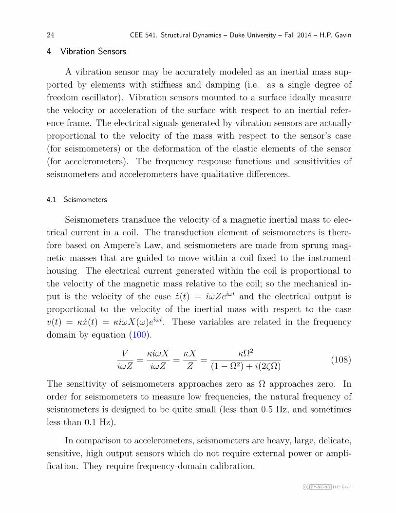
A vibration sensor may be accurately modeled as an inertial mass sup-ported by elements with stiffness and damping (i.e. as a single degree offreedom oscillator). Vibration sensors mounted to a surface ideally measurethe velocity or acceleration of the surface with respect to an inertial refer-ence frame. The electrical signals generated by vibration sensors are actuallyproportional to the velocity of the mass with respect to the sensor’s case(for seismometers) or the deformation of the elastic elements of the sensor(for accelerometers). The frequency response functions and sensitivities ofseismometers and accelerometers have qualitative differences.

4.1 Seismometers

Seismometers transduce the velocity of a magnetic inertial mass to elec-trical current in a coil. The transduction element of seismometers is there-fore based on Ampere’s Law, and seismometers are made from sprung mag-netic masses that are guided to move within a coil fixed to the instrumenthousing. The electrical current generated within the coil is proportional tothe velocity of the magnetic mass relative to the coil; so the mechanical in-put is the velocity of the case z(t) = iωZeiωt and the electrical output isproportional to the velocity of the inertial mass with respect to the casev(t) = κx(t) = κiωX(ω)eiωt. These variables are related in the frequencydomain by equation (100).

V

iωZ= κiωX

iωZ= κX

Z= κΩ2

(1− Ω2) + i(2ζΩ) (108)

The sensitivity of seismometers approaches zero as Ω approaches zero. Inorder for seismometers to measure low frequencies, the natural frequency ofseismometers is designed to be quite small (less than 0.5 Hz, and sometimesless than 0.1 Hz).

In comparison to accelerometers, seismometers are heavy, large, delicate,sensitive, high output sensors which do not require external power or ampli-fication. They require frequency-domain calibration.




4.2 Accelerometers

Accelerometers transduce the deformation of inertially-loaded elastic el-ements within the sensor to an electrical charge, a voltage, or a current.Accelerometers may be designed with many types of transduction elements,including piezo-electric materials, strain-gages, variable capacitance compo-nents, and feed-back stabilization.

In all cases, the mechanical input to the accelerometer is the accelerationof the case z(t) = −ω2Zeiωt, the electrical output is proportional to thedeformation of the spring v(t) = κx(t) = κXeiωt, and these variables arerelated in the frequency domain by

V

−ω2Z= −κ/ω2

n(1− Ω2) + i(2ζΩ) (109)

So the sensitivity of an accelerometer increases with decreasing natural fre-quency.

Piezo-electric accelerometers have natural frequencies in the range of1 kHz to 20 kHz and damping ratios in the range of 0.5% to 1.0%. Be-cause of electrical coupling considerations and the sensitivity of peizo-electricaccelerometers to low-frequency temperature transients, the sensitivity andsignal-to-noise ratio of piezo-electric accelerometers below 1 Hz can be quitepoor.

Micro-machined electro-mechanical silicon (MEMS) accelerometers aremonolithic with their signal-conditioning micro-circuitry. They typically havenatural frequencies in the 100 Hz to 500 Hz range and are accurate down tofrequencies of 0 Hz (constant acceleration, e.g., gravity). These sensors aredamped to a level of about 70% of critical damping.

Force-balance accelerometers utilize feedback circuitry to magneticallystabilize an inertial mass. The force required to stabilize the mass is directlyproportional to the acceleration of the sensor. Such sensors can be made tomeasure accelerations in the µg range down to frequencies of 0 Hz, and havenatural frequencies on the order of 100 Hz, also with damping of about 70%of critical damping.




Accelerometers are typically light, small, and rugged but require electricalpower, amplification, and signal conditioning.

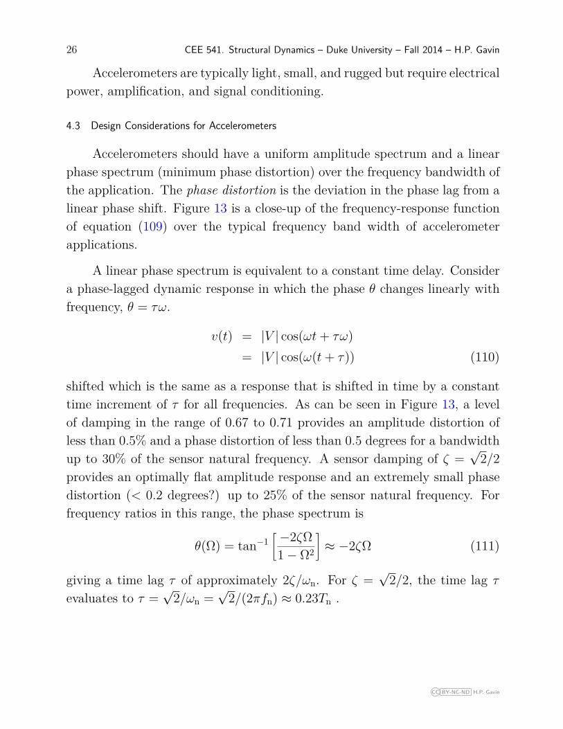
4.3 Design Considerations for Accelerometers

Accelerometers should have a uniform amplitude spectrum and a linearphase spectrum (minimum phase distortion) over the frequency bandwidth ofthe application. The phase distortion is the deviation in the phase lag from alinear phase shift. Figure 13 is a close-up of the frequency-response functionof equation (109) over the typical frequency band width of accelerometerapplications.

A linear phase spectrum is equivalent to a constant time delay. Considera phase-lagged dynamic response in which the phase θ changes linearly withfrequency, θ = τω.

v(t) = |V | cos(ωt+ τω)= |V | cos(ω(t+ τ)) (110)

shifted which is the same as a response that is shifted in time by a constanttime increment of τ for all frequencies. As can be seen in Figure 13, a levelof damping in the range of 0.67 to 0.71 provides an amplitude distortion ofless than 0.5% and a phase distortion of less than 0.5 degrees for a bandwidthup to 30% of the sensor natural frequency. A sensor damping of ζ =

√2/2

provides an optimally flat amplitude response and an extremely small phasedistortion (< 0.2 degrees?) up to 25% of the sensor natural frequency. Forfrequency ratios in this range, the phase spectrum is

θ(Ω) = tan−1[ −2ζΩ1− Ω2

]≈ −2ζΩ (111)

giving a time lag τ of approximately 2ζ/ωn. For ζ =√

2/2, the time lag τ

evaluates to τ =√

2/ωn =√

2/(2πfn) ≈ 0.23Tn .




-1

-0.5

0

0.5

1

0 0.1 0.2 0.3 0.4 0.5

phase d

isto

rtio

n, degre

es


ζ = 0.650ζ = 0.675ζ = 0.707

0.985

0.99

0.995

1

1.005

1.01

1.015

0 0.1 0.2 0.3 0.4 0.5

| X

/ (

ω2 Z

) |

Accelerometer Sensitivity (ω2 Z to X)

ζ = 0.650ζ = 0.675ζ = 0.707

Figure 13. Accelerometer frequency response functions

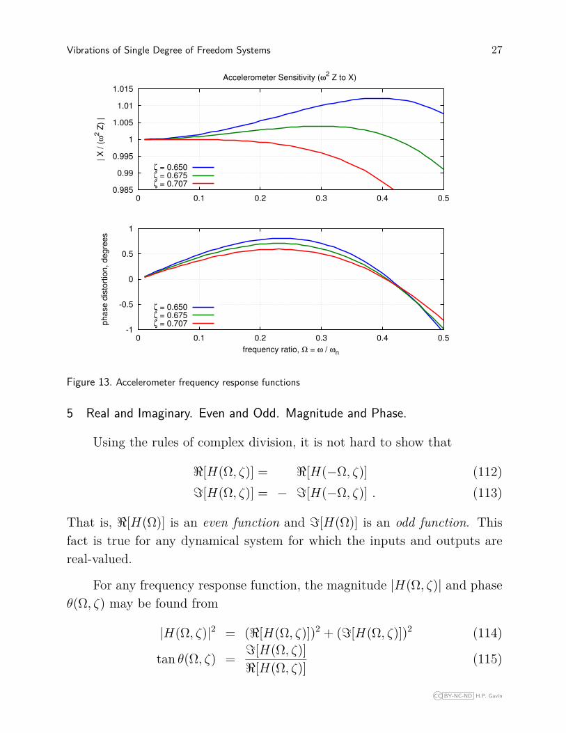
5 Real and Imaginary. Even and Odd. Magnitude and Phase.

Using the rules of complex division, it is not hard to show that

<[H(Ω, ζ)] = <[H(−Ω, ζ)] (112)=[H(Ω, ζ)] = − =[H(−Ω, ζ)] . (113)

That is, <[H(Ω)] is an even function and =[H(Ω)] is an odd function. Thisfact is true for any dynamical system for which the inputs and outputs arereal-valued.

For any frequency response function, the magnitude |H(Ω, ζ)| and phaseθ(Ω, ζ) may be found from

|H(Ω, ζ)|2 = (<[H(Ω, ζ)])2 + (=[H(Ω, ζ)])2 (114)

tan θ(Ω, ζ) = =[H(Ω, ζ)]<[H(Ω, ζ)] (115)




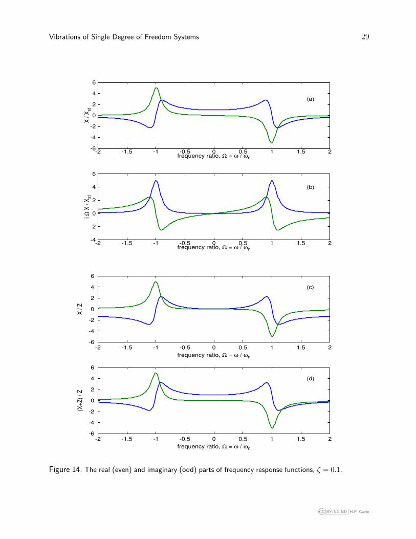
Expressions for the magnitude of various frequency response functionsare given by equations (92), (101), and (102). The magnitude and phase lagof these functions are plotted in Figures 7, 9, and 10. Real and imaginaryparts of H(Ω, ζ) are plotted in Figure 14. Note the following:

• The real and imaginary parts are even and odd, respectively.

• The real part of X/xst (force to response displacement) is zero at Ω = 1.The phase at Ω = 1 is 90 degrees.

• The real part of X/Z (support motion to response motion) is zero atΩ = 1. The phase at Ω = 1 is 90 degrees.

• The imaginary part of iΩX/xst (force to response velocity) is zero atΩ = 1. The phase at Ω = 1 is 90 degrees.

• The real part of iΩX/xst (force to response velocity) is maximum atΩ = 1.

• The real part of iΩX/xst (force to response velocity) is positive for allvalues of Ω.




-4

-2

0

2

4

6

-2 -1.5 -1 -0.5 0 0.5 1 1.5 2

i Ω X

/ X

st


(b)

-6

-4

-2

0

2

4

6

-2 -1.5 -1 -0.5 0 0.5 1 1.5 2

X /

Xst


(a)

-6

-4

-2

0

2

4

6

-2 -1.5 -1 -0.5 0 0.5 1 1.5 2

(X+

Z)

/ Z


(d)

-6

-4

-2

0

2

4

6

-2 -1.5 -1 -0.5 0 0.5 1 1.5 2

X /

Z


(c)

Figure 14. The real (even) and imaginary (odd) parts of frequency response functions, ζ = 0.1.



Documents

Vibrations of Single Degree of Freedom Systemslibvolume3.xyz/.../forcedvibrationsofsingledegreefreedo… · · 2014-05-28Vibrations of Single Degree of Freedom Systems CEE 541