Embed Size (px)
Citation preview
Nonlinear Dyn (2011) 65:109–129DOI 10.1007/s11071-010-9878-0
O R I G I NA L PA P E R
Vibrational self-alignment of a rigid object exploitingfriction
B.G.B. Hunnekens · R.H.B. Fey · A. Shukla ·H. Nijmeijer
Received: 7 April 2010 / Accepted: 22 October 2010 / Published online: 6 November 2010© The Author(s) 2010. This article is published with open access at Springerlink.com
Abstract In this paper, one-dimensional self-align-ment of a rigid object via stick-slip vibrations is stud-ied. The object is situated on a table, which has a pre-scribed periodic motion. Friction is exploited as themechanism to move the object in a desired directionand to stop and self-align the mass at a desired endposition with the smallest possible positioning error.In the modeling and analysis of the system, theory ofdiscontinuous dynamical systems is used. Analytic so-lutions can be derived for a model based on Coulombfriction and an intuitively chosen table accelerationprofile, which allows for a classification of differentpossible types of motion. Local stability and conver-gence is proven for the solutions of the system, if aconstant Coulomb friction coefficient is used. Next,near the desired end position, the Coulomb frictioncoefficient is increased (e.g. by changing the rough-ness of the table surface) in order to stop the object. Inthe transition region from low friction to high frictioncoefficient, it is shown that, under certain conditions,accumulation of the object to a unique end position
B.G.B. Hunnekens · R.H.B. Fey (�) · H. NijmeijerDepartment of Mechanical Engineering, EindhovenUniversity of Technology, P.O. Box 513, 5600 MBEindhoven, The Netherlandse-mail: [email protected]
A. ShuklaDepartment of Mechanical and ManufacturingEngineering, Miami University, EGB 56 Oxford, OH45056, USA
occurs. This behavior can be studied analytically anda mapping is given for subsequent stick positions.
Keywords Self-alignment · Friction · Stick-slipvibrations · Accumulation position · Positioning
1 Introduction
Accurate positioning of objects is very important in in-dustrial applications, e.g. in printer heads, CD-players,pick-and-place machines, welding robots, etc. Usu-ally, the positioning and tracking problem is tackledusing closed-loop control using feedback to asymptot-ically stabilize the error dynamics. In this paper, theself-aligning positioning problem will be addressed.A rigid object is placed on a table which will besubmitted to a periodic motion profile. Friction-basedstick-slip vibrations will be used as a mechanism bywhich the rigid object (in this paper also referred toas: the mass) will move in a desired direction. By lo-cally increasing the friction the mass will self-align ata desired end position.
Some (simplified) friction models for dynamics andcontrol applications have been studied e.g. in [1]. Anextensive treatment of friction modeling can be foundin [2]. In literature, the dry-friction oscillator withCoulomb friction has received much attention. In thissystem, a mass experiencing Coulomb friction is con-nected to the world by a spring and a viscous damper,while an external periodic force acts on the mass, see
110 B.G.B. Hunnekens et al.
[6, 13], and [21]. As early as 1930, Den Hartog gavethe exact solution of a single degree of freedom har-monic oscillator with dry friction [6]. Cases where thestatic and dynamical friction coefficients are not equalto each other have been studied in [20]. Also, describ-ing function approaches have been used to analyze thebehavior of this type of system, see e.g. [7]. In [8], themethod of averaging is used to analyze high-frequencyvibration-induced movements of a mass between twolayers of different friction, while in [23] the methodof direct separation of motion (see [3]) is used to cal-culate equilibrium speeds (including zero speed) of amass on a table vibrating at high frequency. In [24],analytical approximations for stick-slip vibration am-plitudes are derived for the classical mass-on-moving-belt system. For the same system, in [10], bifurcationsare studied, which are non-standard due to the discon-tinuous behavior of the dry friction force. In [5], thebifurcations associated with the appearance of stick-slip vibrations are studied using a state variable fric-tion law for a mass on a fixed horizontal surface, mov-ing under the influence of a horizontal force trans-mitted by a linear spring whose other end is movingwith constant velocity. A method of calculating ex-act analytic solutions for parts of the oscillation cy-cles, which are ‘stitched’ together, has been used in[4]; vibration-induced motions of a mass on a frictionplane are studied, and optimal parameter values, forwhich maximum mean velocity is reached, have beendetermined.
Self-alignment of microparts is studied in [19],where the self-alignment is achieved using liquidsurface tension. In [9], resonant magnetic micro-agents are used to move micro-robots using mag-netic fields and vision-feedback for positioning ap-plications. Modeling and closed-loop control of a2-DOF micro-positioning device, using stick-slip mo-tion based on piezoelectric materials, is treated in [17].The work in [18] studies the use of a planar manipula-tor to position multiple objects on a vibrating surfaceusing the frictional forces along with feedback control.
An important motivation for using self-alignmentcompared to conventional closed-loop control is to re-duce cost by eliminating the need for feedback con-trol equipment. Possible practical applications couldinclude parts feeding, automated assembly, or inspec-tion of parts. To the best knowledge of the authors,there is no literature available in which friction is ex-ploited to move a mass in a desired direction and in
which a mass self-aligns using friction, which moti-vates this study.
The paper is structured as follows. In Sect. 2, thetwo major objectives of this paper will be discussed.The focus in Sect. 3 will be on the dynamical model.The stopping regime will be discussed in detail. Thetable trajectory design will be studied in Sect. 4. InSect. 5, the classification of different types of motionwill be introduced. Local stability and convergence ofsolutions will be proven in Sect. 6. The positioningaccuracy obtained, when the mass stops, will be inves-tigated in Sect. 7. Finally, in Sect. 8, conclusions andsome recommendations for future work will be given.
2 Problem formulation
The basic objective of this paper is to design a self-positioning method, in which friction is used to movea mass on a table in a desired direction, using dry fric-tion and periodic motion of the table. For the table,a suitable periodic motion profile must be designedthat achieves this as fast as possible, given some actua-tor constraints. Furthermore, the mass needs to be po-sitioned/stopped at a desired end position accurately.Summarizing, the two main objectives of this researchare:
– Design a periodic table displacement signal y(t )
such that the mass travels to a desired end locationxd in the smallest possible process time Tp , whereTp = min(W ) and W ∈ {t ≥ 0|x(t ) = xd}.
– Minimize the positioning error |�xd | of the end po-sition of the mass; in other words, minimize theinterval [xd − �xd, xd + �xd ], in which the massstops.
In this paper, the ∼ above a quantity means thatthe quantity is in SI units, whereas for dimensionlessquantities the ∼ will be omitted.
3 Modeling the system dynamics
3.1 Dynamical model
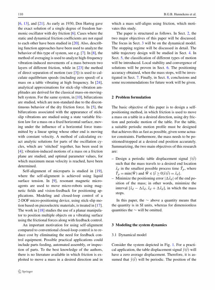
Consider the system depicted in Fig. 1. For a practi-cal application, the table displacement signal y(t ) willhave a zero average displacement. Therefore, it is as-sumed that y(t ) will be periodic. The position of the
Vibrational self-alignment of a rigid object exploiting friction 111
Fig. 1 Schematic of thesystem
mass relative to the table is denoted by x(t ). Note thatan arbitrary position on the table can be chosen as theorigin of x(t ). Between the table and the mass m, aCoulomb friction force Ff with friction coefficient μ
exists, which mathematically can be described as fol-lows (see e.g. [11]):
Ff ∈ μmg Sign( ˙x) (1)
where g is the acceleration due to gravity, and Sign( ˙x)
is the set-valued sign function, defined by:
Sign( ˙x) =
⎧⎪⎨
⎪⎩
{1} if ˙x > 0
[−1,1] if ˙x = 0
{−1} if ˙x < 0
(2)
Note that in case the mass sticks to the table (so˙x = 0), the friction force can take values in the range[−μmg,μmg]. This allows the mass to stick to the ta-ble as long as the external force acting on the massis small enough. Using Newton’s second law it isstraightforward to derive the equation of motion forthe mass:
−Ff = m( ¨x + ¨y)
(3)
If the relative velocity of the mass is zero ( ˙x = 0)and the external force acting on the mass is smallenough (i.e. |m ¨y| < μmg), the friction force will bal-ance this external force (−Ff = m ¨y) resulting in¨x = 0, i.e. in sticking of the mass. If the externalforce is larger than the maximum friction force (i.e.|m ¨y| > μmg), the mass will start to slip, resulting in˙x �= 0 and Ff = μmg Sign( ˙x).
3.2 Dimensionless dynamical model
The equation of motion derived in the previous sec-tion will be made dimensionless to obtain a modelwhich incorporates a minimum number of parameters.
A characteristic length scale L and a characteristictime scale T need to be introduced. The dimensionlesslength scales x and y and dimensionless time scale t
are defined in the following way:
x = x/L, y = y/L, t = t/T (4)
Also, a dimensionless differential operator is de-
fined as ′ = d/dt . If we choose T =√
L/μg, theequation of motion (3) can be written in dimension-less form as:
−Ff = x′′ + y′′ (5)
where Ff = Ff /μmg ∈ Sign(x′), using (1). Note that(5) can now be written as:
−Sign(x′) � x′′ + y′′ (6)
The dimensionless condition for sticking of themass (x′ = 0) now reduces to |y′′| < 1.
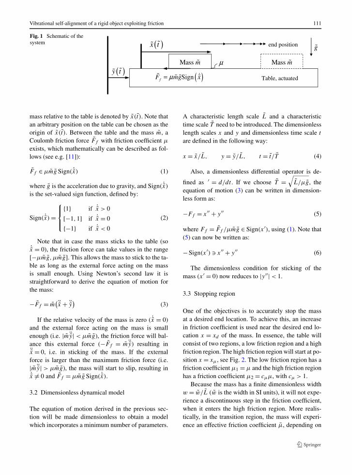
3.3 Stopping region
One of the objectives is to accurately stop the massat a desired end location. To achieve this, an increasein friction coefficient is used near the desired end lo-cation x = xd of the mass. In essence, the table willconsist of two regions, a low friction region and a highfriction region. The high friction region will start at po-sition x = xμ, see Fig. 2. The low friction region has afriction coefficient μ1 = μ and the high friction regionhas a friction coefficient μ2 = cμμ, with cμ > 1.
Because the mass has a finite dimensionless widthw = w/L (w is the width in SI units), it will not expe-rience a discontinuous step in the friction coefficient,when it enters the high friction region. More realis-tically, in the transition region, the mass will experi-ence an effective friction coefficient μ, depending on
112 B.G.B. Hunnekens et al.
Fig. 2 Schematic of thetable with two regions, oneregion with low frictioncoefficient μ1 and anotherregion with high frictioncoefficient μ2
the distribution of the weight of the mass over the lowfriction region and the high friction region:
μ(z) = w − z
wμ1 + z
wμ2 = w + (cμ − 1)z
wμ (7)
where z is the portion of the mass on the high fric-tion region, see Fig. 2. Note that z is bounded by0 ≤ z ≤ w. This constraint can conveniently be for-mulated using a min-max formulation:
z = min(max(x − xμ,0),w) (8)
The friction coefficient μ that the mass experi-ences, thus depends on the position x of the mass. Notethat in the transition region, using (7) and (8), the fric-tion coefficient can be written as follows:
μ(x) = μ
(
1 + cμ − 1
w(x − xμ)
)
if xμ ≤ x ≤ xμ + w (9)
In all simulation results presented throughout thispaper, it is assumed that the mass does not tip over, i.e.it is assumed that the mass will remain in full contactwith the table, so that the equation of motion (6) re-mains valid. In general, this will be valid for an objectthe height of which is relatively small with respect toits width w.
4 Table trajectory design
The design of the table motion profile will be dis-cussed in this section. First, in Sect. 4.1, a simulationmethod called the time-stepping method will be dis-cussed. In Sect. 4.2, an example of a stick-slip mo-tion of the mass, calculated using the time-stepping
method, will be shown. An objective function will beintroduced in Sect. 4.3, which is used in Sect. 4.4 todesign a suitable table excitation signal.
4.1 Simulation method
The system under study exhibits dry friction, whichmakes it a nonlinear system with unilateral con-straints [12]. There are different methods that can beused to simulate these kind of systems. Time-steppingis an efficient method for numerically solving theequations describing the dynamics of systems withunilateral constraints. A thorough mathematical de-scription of time-stepping method can be found in[11] and [22]. In contrast to, for example, event-driventechniques, in time-stepping it is not necessary to de-tect every event (e.g. a stick-slip transition). The so-lution is computed using fixed time-steps forward intime. The time-stepping method of Moreau [14] isused as the integration routine in this paper. A fixed-point iteration is carried out to solve for the unknownvelocity in the system at every time-step. This veloc-ity is used to estimate the position at the end of thetime-step.
4.2 Example of stick-slip motion
An example of a simulated response using time-stepping is shown in Fig. 3. Note that the time-stepping routine does not explicitly solve for the ac-celeration x′′(t) of the mass. A periodic excitationsignal consisting of a sequence of second order poly-nomials was initially used for the table displacementsignal y(t). Intuitively, the table should move slowlyin the desired direction dragging the mass along, andfast in the opposite direction, resulting in slipping of
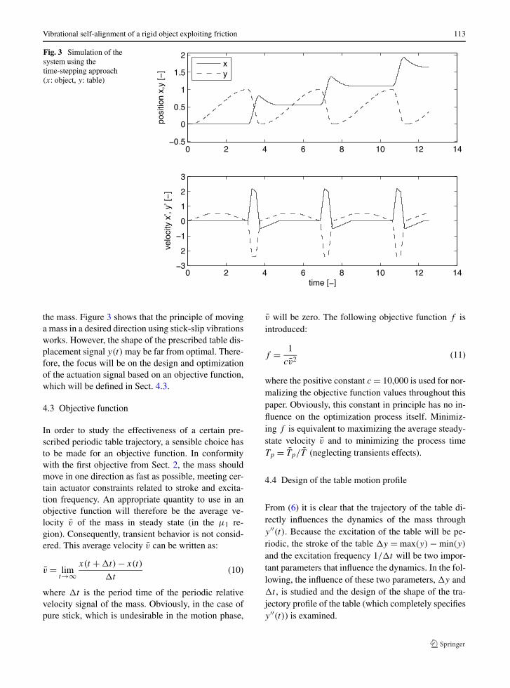
Vibrational self-alignment of a rigid object exploiting friction 113
Fig. 3 Simulation of thesystem using thetime-stepping approach(x: object, y: table)
the mass. Figure 3 shows that the principle of movinga mass in a desired direction using stick-slip vibrationsworks. However, the shape of the prescribed table dis-placement signal y(t) may be far from optimal. There-fore, the focus will be on the design and optimizationof the actuation signal based on an objective function,which will be defined in Sect. 4.3.
4.3 Objective function
In order to study the effectiveness of a certain pre-scribed periodic table trajectory, a sensible choice hasto be made for an objective function. In conformitywith the first objective from Sect. 2, the mass shouldmove in one direction as fast as possible, meeting cer-tain actuator constraints related to stroke and excita-tion frequency. An appropriate quantity to use in anobjective function will therefore be the average ve-locity v of the mass in steady state (in the μ1 re-gion). Consequently, transient behavior is not consid-ered. This average velocity v can be written as:
v = limt→∞
x(t + �t) − x(t)
�t(10)
where �t is the period time of the periodic relativevelocity signal of the mass. Obviously, in the case ofpure stick, which is undesirable in the motion phase,
v will be zero. The following objective function f isintroduced:
f = 1
cv2(11)
where the positive constant c = 10,000 is used for nor-malizing the objective function values throughout thispaper. Obviously, this constant in principle has no in-fluence on the optimization process itself. Minimiz-ing f is equivalent to maximizing the average steady-state velocity v and to minimizing the process timeTp = Tp/T (neglecting transients effects).
4.4 Design of the table motion profile
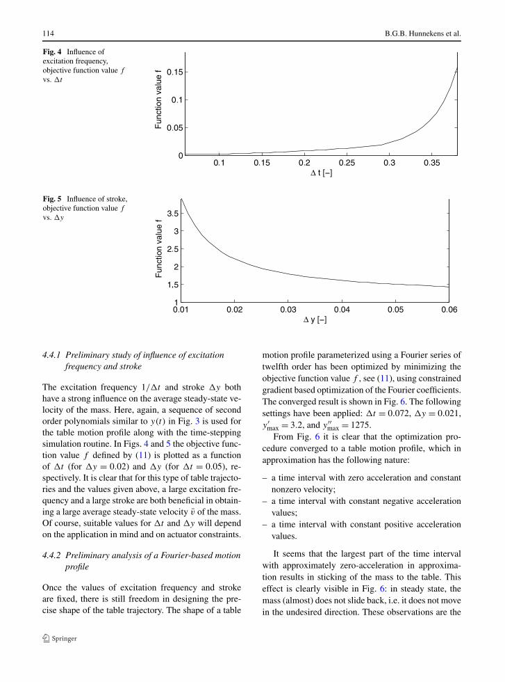
From (6) it is clear that the trajectory of the table di-rectly influences the dynamics of the mass throughy′′(t). Because the excitation of the table will be pe-riodic, the stroke of the table �y = max(y) − min(y)
and the excitation frequency 1/�t will be two impor-tant parameters that influence the dynamics. In the fol-lowing, the influence of these two parameters, �y and�t , is studied and the design of the shape of the tra-jectory profile of the table (which completely specifiesy′′(t)) is examined.
114 B.G.B. Hunnekens et al.
Fig. 4 Influence ofexcitation frequency,objective function value f
vs. �t
Fig. 5 Influence of stroke,objective function value f
vs. �y
4.4.1 Preliminary study of influence of excitationfrequency and stroke
The excitation frequency 1/�t and stroke �y bothhave a strong influence on the average steady-state ve-locity of the mass. Here, again, a sequence of secondorder polynomials similar to y(t) in Fig. 3 is used forthe table motion profile along with the time-steppingsimulation routine. In Figs. 4 and 5 the objective func-tion value f defined by (11) is plotted as a functionof �t (for �y = 0.02) and �y (for �t = 0.05), re-spectively. It is clear that for this type of table trajecto-ries and the values given above, a large excitation fre-quency and a large stroke are both beneficial in obtain-ing a large average steady-state velocity v of the mass.Of course, suitable values for �t and �y will dependon the application in mind and on actuator constraints.
4.4.2 Preliminary analysis of a Fourier-based motionprofile
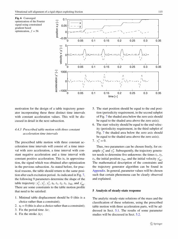
Once the values of excitation frequency and strokeare fixed, there is still freedom in designing the pre-cise shape of the table trajectory. The shape of a table
motion profile parameterized using a Fourier series oftwelfth order has been optimized by minimizing theobjective function value f , see (11), using constrainedgradient based optimization of the Fourier coefficients.The converged result is shown in Fig. 6. The followingsettings have been applied: �t = 0.072, �y = 0.021,y′
max = 3.2, and y′′max = 1275.
From Fig. 6 it is clear that the optimization pro-cedure converged to a table motion profile, which inapproximation has the following nature:
– a time interval with zero acceleration and constantnonzero velocity;
– a time interval with constant negative accelerationvalues;
– a time interval with constant positive accelerationvalues.
It seems that the largest part of the time intervalwith approximately zero-acceleration in approxima-tion results in sticking of the mass to the table. Thiseffect is clearly visible in Fig. 6: in steady state, themass (almost) does not slide back, i.e. it does not movein the undesired direction. These observations are the
Vibrational self-alignment of a rigid object exploiting friction 115
Fig. 6 Convergedoptimization of the Fouriersignal using constrainedgradient basedoptimization, f = 56
motivation for the design of a table trajectory gener-ator incorporating these three distinct time intervalswith constant acceleration values. This will be dis-cussed in detail in the next subsection.
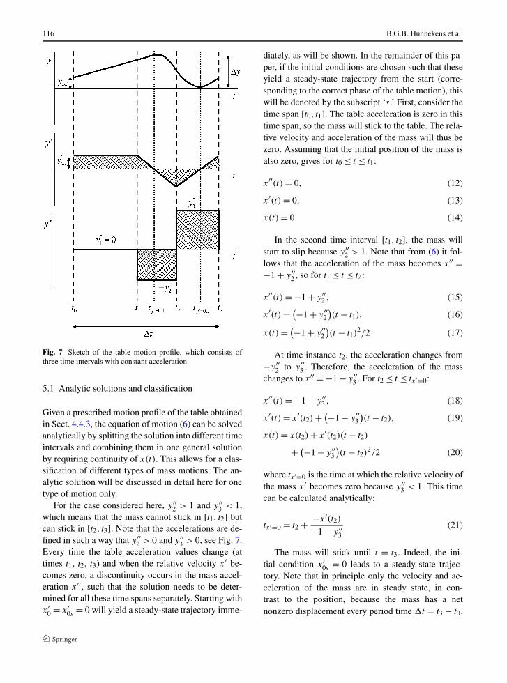
4.4.3 Prescribed table motion with three constantacceleration time intervals
The prescribed table motion with three constant ac-celeration time intervals will consist of: a time inter-val with zero acceleration, a time interval with con-stant negative acceleration and a time interval withconstant positive acceleration. This is, in approxima-tion, the signal which was obtained after optimizationin the previous subsection. As stated before, for prac-tical reasons, the table should return to the same posi-tion after each excitation period. As indicated in Fig. 7,the following 9 parameters determine the shape of thetable trajectory: y′′
1 , y′′2 , y′′
3 , t0, t1, t2, t3, yini, and y′ini.
There are some constraints to the table motion profilethat need to be satisfied:
1. Minimal table displacement should be 0 (this is achoice rather than a constraint);
2. t0 = 0 (this is also a choice rather than a constraint);3. Fix the period time �t ;4. Fix the stroke �y;
5. The start position should be equal to the end posi-tion (periodicity requirement, in the second subplotof Fig. 7 the shaded area below the zero axis shouldbe equal to the shaded area above the zero axis);
6. The start velocity should be equal to the end veloc-ity (periodicity requirement, in the third subplot ofFig. 7 the shaded area below the zero axis shouldbe equal to the shaded area above the zero axis);
7. y′′1 = 0.
Thus, two parameters can be chosen freely, for ex-ample y′′
2 and y′′3 . Subsequently, the trajectory genera-
tor needs to determine five unknowns: the times t1, t2,t3, the initial position yini, and the initial velocity y′
ini.The mathematical description of the constraints andthe trajectory generator algorithm can be found inAppendix. In general, parameter values will be chosensuch that certain phenomena can be clearly observedand explained.
5 Analysis of steady-state response
The analytic steady-state solutions of the mass and theclassification of these solutions, using the prescribedtable motion with three acceleration parts, will be ad-dressed in Sect. 5.1. The results of some parameterstudies will be discussed in Sect. 5.2.
116 B.G.B. Hunnekens et al.
Fig. 7 Sketch of the table motion profile, which consists ofthree time intervals with constant acceleration
5.1 Analytic solutions and classification
Given a prescribed motion profile of the table obtainedin Sect. 4.4.3, the equation of motion (6) can be solvedanalytically by splitting the solution into different timeintervals and combining them in one general solutionby requiring continuity of x(t). This allows for a clas-sification of different types of mass motions. The an-alytic solution will be discussed in detail here for onetype of motion only.
For the case considered here, y′′2 > 1 and y′′
3 < 1,which means that the mass cannot stick in [t1, t2] butcan stick in [t2, t3]. Note that the accelerations are de-fined in such a way that y′′
2 > 0 and y′′3 > 0, see Fig. 7.
Every time the table acceleration values change (attimes t1, t2, t3) and when the relative velocity x′ be-comes zero, a discontinuity occurs in the mass accel-eration x′′, such that the solution needs to be deter-mined for all these time spans separately. Starting withx′
0 = x′0s = 0 will yield a steady-state trajectory imme-
diately, as will be shown. In the remainder of this pa-per, if the initial conditions are chosen such that theseyield a steady-state trajectory from the start (corre-sponding to the correct phase of the table motion), thiswill be denoted by the subscript ‘s.’ First, consider thetime span [t0, t1]. The table acceleration is zero in thistime span, so the mass will stick to the table. The rela-tive velocity and acceleration of the mass will thus bezero. Assuming that the initial position of the mass isalso zero, gives for t0 ≤ t ≤ t1:
x′′(t) = 0, (12)
x′(t) = 0, (13)
x(t) = 0 (14)
In the second time interval [t1, t2], the mass willstart to slip because y′′
2 > 1. Note that from (6) it fol-lows that the acceleration of the mass becomes x′′ =−1 + y′′
2 , so for t1 ≤ t ≤ t2:
x′′(t) = −1 + y′′2 , (15)
x′(t) = (−1 + y′′2
)(t − t1), (16)
x(t) = (−1 + y′′2
)(t − t1)
2/2 (17)
At time instance t2, the acceleration changes from−y′′
2 to y′′3 . Therefore, the acceleration of the mass
changes to x′′ = −1 − y′′3 . For t2 ≤ t ≤ tx′=0:
x′′(t) = −1 − y′′3 , (18)
x′(t) = x′(t2) + (−1 − y′′3
)(t − t2), (19)
x(t) = x(t2) + x′(t2)(t − t2)
+ (−1 − y′′3
)(t − t2)
2/2 (20)
where tx′=0 is the time at which the relative velocity ofthe mass x′ becomes zero because y′′
3 < 1. This timecan be calculated analytically:
tx′=0 = t2 + −x′(t2)−1 − y′′
3(21)
The mass will stick until t = t3. Indeed, the ini-tial condition x′
0s = 0 leads to a steady-state trajec-tory. Note that in principle only the velocity and ac-celeration of the mass are in steady state, in con-trast to the position, because the mass has a netnonzero displacement every period time �t = t3 − t0.
Vibrational self-alignment of a rigid object exploiting friction 117
For tx′=0 ≤ t ≤ t3:
x′′(t) = 0, (22)
x′(t) = 0, (23)
x(t) = x(tx′=0) (24)
Simulations and solving different cases analyticallypoint out that in the μ1 region 5 different types ofsteady-state responses can occur, depending on themagnitudes of y′′
2 and y′′3 , see Table 1.
Note that the analytic solution for case 1 has beenderived above. For cases 1–4, the period of the relativevelocity response is equal to the excitation period �t .
The analytic solutions of cases 2–5 can be derivedin an equivalent manner as was done above for thecase 1 type of motion. Determination of the result-ing case can be done a priori by following the flow
Table 1 Table showing possible types of steady-state responses
Case Description (Un)desirable?
1 Stick-slip with Desirable
x′(t) ≥ 0,∀t
2 Stick-slip with Undesirable
x′(t) ≤ 0,∀t
3 General stick-slip Acceptable if v > 0
4 Slip-slip Acceptable if v > 0
5 Pure stick Only desirable
(no relative motion) in stopping region
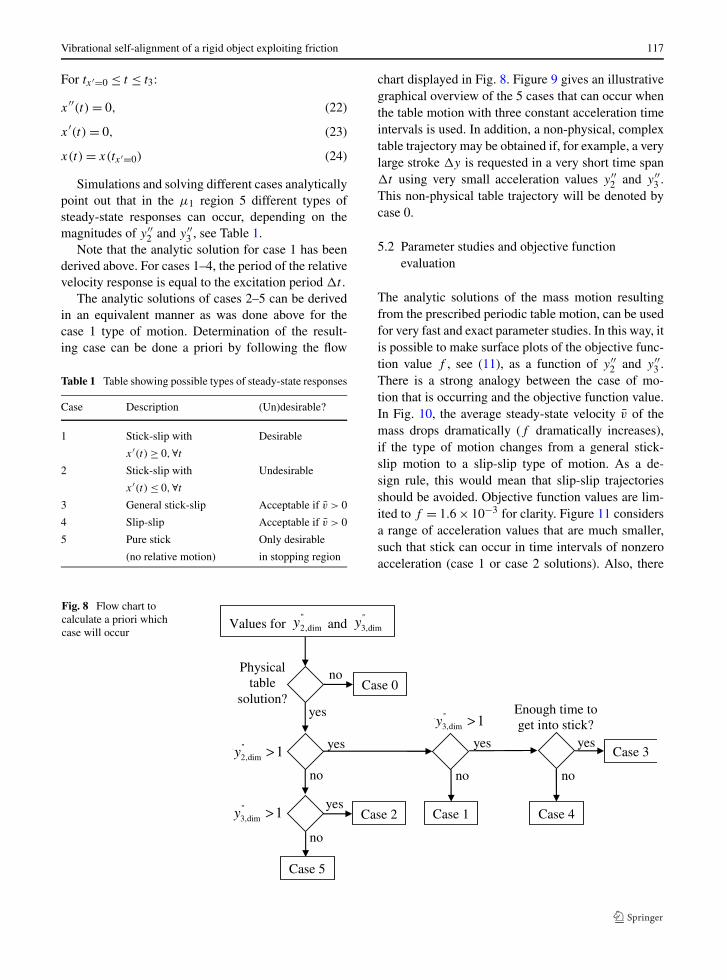
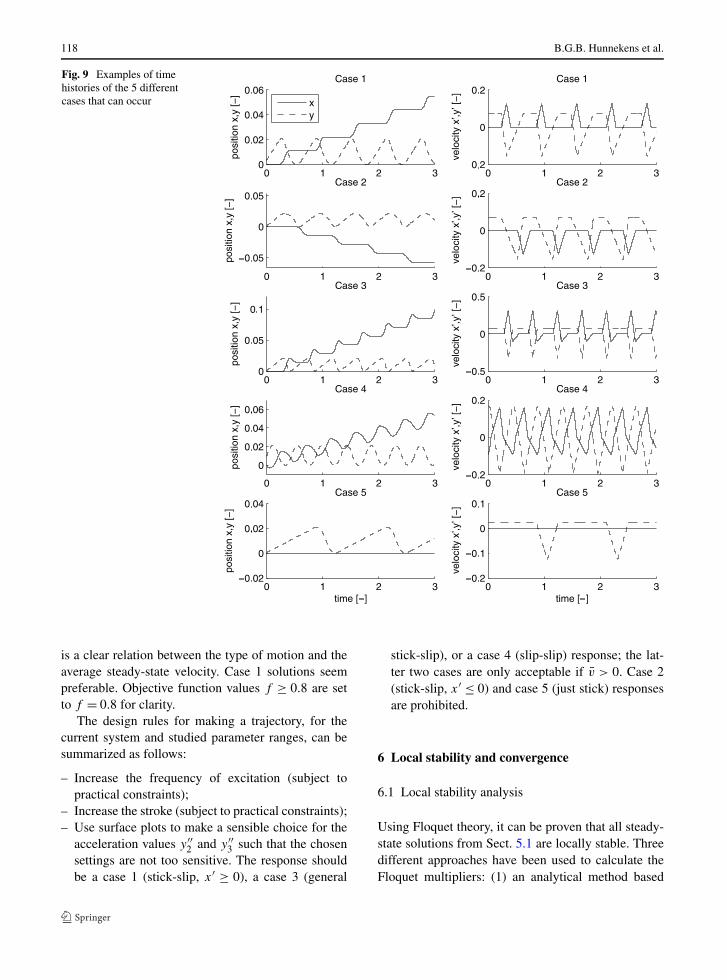
chart displayed in Fig. 8. Figure 9 gives an illustrativegraphical overview of the 5 cases that can occur whenthe table motion with three constant acceleration timeintervals is used. In addition, a non-physical, complextable trajectory may be obtained if, for example, a verylarge stroke �y is requested in a very short time span�t using very small acceleration values y′′
2 and y′′3 .
This non-physical table trajectory will be denoted bycase 0.
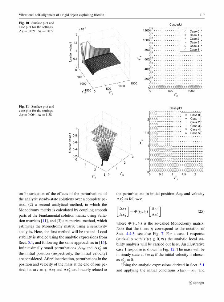
5.2 Parameter studies and objective functionevaluation
The analytic solutions of the mass motion resultingfrom the prescribed periodic table motion, can be usedfor very fast and exact parameter studies. In this way, itis possible to make surface plots of the objective func-tion value f , see (11), as a function of y′′
2 and y′′3 .
There is a strong analogy between the case of mo-tion that is occurring and the objective function value.In Fig. 10, the average steady-state velocity v of themass drops dramatically (f dramatically increases),if the type of motion changes from a general stick-slip motion to a slip-slip type of motion. As a de-sign rule, this would mean that slip-slip trajectoriesshould be avoided. Objective function values are lim-ited to f = 1.6 × 10⁻³ for clarity. Figure 11 considersa range of acceleration values that are much smaller,such that stick can occur in time intervals of nonzeroacceleration (case 1 or case 2 solutions). Also, there
Fig. 8 Flow chart tocalculate a priori whichcase will occur
118 B.G.B. Hunnekens et al.
Fig. 9 Examples of timehistories of the 5 differentcases that can occur
is a clear relation between the type of motion and theaverage steady-state velocity. Case 1 solutions seempreferable. Objective function values f ≥ 0.8 are setto f = 0.8 for clarity.
The design rules for making a trajectory, for thecurrent system and studied parameter ranges, can besummarized as follows:
– Increase the frequency of excitation (subject topractical constraints);
– Increase the stroke (subject to practical constraints);– Use surface plots to make a sensible choice for the
acceleration values y′′2 and y′′
3 such that the chosensettings are not too sensitive. The response shouldbe a case 1 (stick-slip, x′ ≥ 0), a case 3 (general
stick-slip), or a case 4 (slip-slip) response; the lat-ter two cases are only acceptable if v > 0. Case 2(stick-slip, x′ ≤ 0) and case 5 (just stick) responsesare prohibited.
6 Local stability and convergence
6.1 Local stability analysis
Using Floquet theory, it can be proven that all steady-state solutions from Sect. 5.1 are locally stable. Threedifferent approaches have been used to calculate theFloquet multipliers: (1) an analytical method based
Vibrational self-alignment of a rigid object exploiting friction 119
Fig. 10 Surface plot andcase plot for the settings�y = 0.021, �t = 0.072
Fig. 11 Surface plot andcase plot for the settings�y = 0.064, �t = 1.38
on linearization of the effects of the perturbations ofthe analytic steady-state solutions over a complete pe-riod, (2) a second analytical method, in which theMonodromy matrix is calculated by coupling smoothparts of the Fundamental solution matrix using Salta-tion matrices [11], and (3) a numerical method, whichestimates the Monodromy matrix using a sensitivityanalysis. Here, the first method will be treated. Localstability is studied using the analytic expressions fromSect. 5.1, and following the same approach as in [15].Infinitesimally small perturbations �x0 and �x′
0 onthe initial position (respectively, the initial velocity)are considered. After linearization, perturbations in theposition and velocity of the mass at the end of one pe-riod, i.e. at t = t3, �x3 and �x′
3, are linearly related to
the perturbations in initial position �x0 and velocity�x′
0 as follows:
[�x3
�x′3
]
= Φ(t3, t0)
[�x0
�x′0
]
(25)
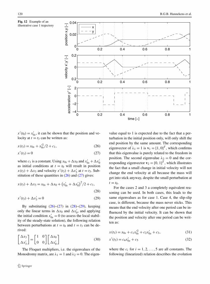
where Φ(t3, t0) is the so-called Monodromy matrix.Note that the times ti correspond to the notation ofSect. 4.4.3; see also Fig. 7. For a case 1 response(stick-slip with x′(t) ≥ 0,∀t) the analytic local sta-bility analysis will be carried out here. An illustrativecase 1 response is shown in Fig. 12. The mass will bein steady state at t = t0 if the initial velocity is chosenas x′
0s = 0.Using the analytic expressions derived in Sect. 5.1
and applying the initial conditions x(t0) = x0s and
120 B.G.B. Hunnekens et al.
Fig. 12 Example of anillustrative case 1 trajectory
x′(t0) = x′0s , it can be shown that the position and ve-
locity at t = t3 can be written as:
x(t3) = x0s + x′20s/2 + c1, (26)
x′(t3) = 0 (27)
where c1 is a constant. Using x0s +�x0 and x′0s +�x′
0as initial conditions at t = t0 will result in positionx(t3) + �x3 and velocity x′(t3) + �x′
3 at t = t3. Sub-stitution of these quantities in (26) and (27) gives:
x(t3) + �x3 = x0s + �x0 + (x′
0s + �x′0
)2/2 + c1,
(28)
x′(t3) + �x′3 = 0 (29)
By substituting (26)–(27) in (28)–(29), keepingonly the linear terms in �x0 and �x′
0, and applyingthe initial condition x′
0s = 0 (to assess the local stabil-ity of the steady-state solution), the following relationbetween perturbations at t = t0 and t = t3 can be de-rived:[
�x3
�x′3
]
=[
1 0
0 0
][�x0
�x′0
]
(30)
The Floquet multipliers, i.e. the eigenvalues of theMonodromy matrix, are λ1 = 1 and λ2 = 0. The eigen-
value equal to 1 is expected due to the fact that a per-turbation in the initial position only, will only shift theend position by the same amount. The correspondingeigenvector of λ1 = 1 is v1 = [1,0]T , which confirmsthat this eigenvalue is purely related to the freedom inposition. The second eigenvalue λ2 = 0 and the cor-responding eigenvector v2 = [0,1]T , which illustratesthe fact that a small change in initial velocity will notchange the end velocity at all because the mass willget into stick anyway, despite the small perturbation att = t0.
For the cases 2 and 3 a completely equivalent rea-soning can be used. In both cases, this leads to thesame eigenvalues as for case 1. Case 4, the slip-slipcase, is different, because the mass never sticks. Thismeans that the end velocity after one period can be in-fluenced by the initial velocity. It can be shown thatthe position and velocity after one period can be writ-ten as:
x(t3) = x0s + c1x′20s + c2x
′0s + c3, (31)
x′(t3) = c4x′0s + c5 (32)
where the ci for i = 1,2, . . . ,5 are all constants. Thefollowing (linearized) relation describes the evolution
Vibrational self-alignment of a rigid object exploiting friction 121
of small perturbations �x0, �x′0 on the initial condi-
tions:[
�x3
�x′3
]
=[
1 2c1x′0s + c2
0 c4
][�x0
�x′0
]
(33)
The Floquet multipliers can be shown to be λ1 = 1,which again represents the freedom in position, andλ2 = c4 = ((y′′
2 − 1)(y′′3 − 1))/((y′′
2 + 1)(y′′3 + 1)).
Note that this eigenvalue is always positive andsmaller than 1 (so within the unit circle) becausey′′i > 1 for i = 2,3 in the slip-slip case.
The local stability analysis presented in this sec-tion has shown that, besides the fact that the responsecan be shifted in position, the remaining dynamics areall locally asymptotically stable. The analysis usingSaltation matrices to compute the Monodromy matrixgives identical results. The method using numerical es-timation using a sensitivity analysis gives a good ap-proximation of the exact analytical results.
6.2 Convergence
In this subsection, convergence of the relative veloc-ity solutions x′ will be proven, which also proves thatthe solution converges to a unique velocity solutionin steady state, independent of the initial conditions.The (dimensionless) relative velocity is here denotedby v = x′. In terms of the relative velocity, the dynam-ics is described by (see (6)):
v′ ∈ −Sign(v) − y′′(t) (34)
Now consider two trajectories, v1(t, t0, v10) andv2(t, t0, v20), with different initial conditions v10 andv20 at t = t0, and consider the following Lyapunovfunction:
V (v1, v2) = (v1 − v2)2
2(35)
The time derivative of this Lyapunov function alongsolutions of the system can be written as follows [16]:
V ′(v1, v2) = (v1 − v2)(v′
1 − v′2
)
∈ −(v1 − v2)(Sign(v1) − Sign(v2)) (36)
≤ 0
If v1 and v2 are both positive or both negative, thenV ′ = 0. Therefore, V ′ is only negative semi-definite
and convergence is not proven yet. Let v1 ∈ Sign(v1)
and v2 ∈ Sign(v2), see (2). Now, it can be shown thatif v1 = v2 and v1(tA) �= v2(tA) at a certain time t = tA(otherwise convergence has already occurred), therewill always be a time tB > tA, for which v1 �= v2, re-sulting in further decrease of V . Consider the situationin which v1 = v2. For both trajectories the accelera-tion v′
i will be equal, see (34). Both trajectories willeventually reach zero velocity vi = 0. To see this, con-sider (34). The excitation signal y′′(t) is periodic andover a single period �t it has an average accelerationequal to zero, such that its net effect on the velocityx′ of the mass over one period time �t is zero. Thisis shown by integrating (34) over one period time �t ,for v �= 0:
v(t + �t) − v(t) = −∫ t+�t
t
(Sign(v) + y′′(t)
)dt
= −∫ t+�t
t
Sign(v) dt (37)
The term −Sign(v) will force the relative veloc-ity of the mass to v = 0, which will occur at somepoint in time. After the trajectory reaches v = 0, themass can stick or slip, depending on the value of theacceleration y′′ of the table. At the moment, one ofthe trajectories reaches v = 0, v1 �= v2, and V ′ < 0,which means that v1 and v2 will approach each other.This will last until a point in time is reached at whichv1 = v2 again, and the whole process will repeat it-self. Eventually, for cases 1–3 solutions, in finite timea point will be reached at which v1 = v2 = 0. Fromthis time onwards, both velocity signals are fully con-verged, i.e. are equal to each other. In case of a case4 solution, the mass will never stick, and v1 = v2 = 0will be reached in the limit t → ∞.
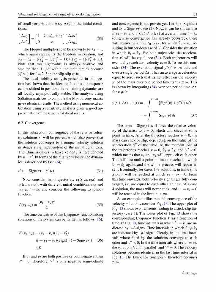
As an example to illustrate this convergence of thevelocity solutions, consider Fig. 13. The upper plot ofFig. 13 shows two transients leading to a stick-slip tra-jectory (case 1). The lower plot of Fig. 13 shows thecorresponding Lyapunov function V as a function oftime. In Fig. 13, time intervals in which v1 = v2 are in-dicated by ‘=’-signs. Time intervals in which v1 �= v2
are indicated by ‘ �=’-signs. Clearly, in the time inter-vals where v1 �= v2, the solutions converge to eachother and V ′ < 0. In the time intervals where v1 = v2,the solutions ‘run in parallel’ and V ′ = 0. The velocitysolutions become identical in the last time interval inFig. 13. The Lyapunov function V therefore becomeszero.
122 B.G.B. Hunnekens et al.
Fig. 13 Illustration ofconvergence of velocitysolutions
Summarizing, although the time derivative of theLyapunov function is only negative semi-definite, ithas been shown that in the time intervals in whichV ′ = 0 the solutions evolve in such a way that alwaysa time interval in which V ′ < 0 will be reached. Thisproves that the two solutions v1 and v2 will convergeto each other. Therefore, the steady-state solution interms of velocity is unique and is independent of theinitial velocity of the mass. In other words, dependingon the system parameters, different types of steady-state motion occur as discussed in Sect. 5.1. However,each steady-state solution is unique. There are no co-existing steady-state solutions.
7 Positioning accuracy in the stopping phase
For stopping and accurate positioning of the mass, anincreased friction coefficient μ2, as described earlierin Sect. 3.3, is used. Depending on the weight dis-tribution of the mass over the two table regions withtwo different Coulomb friction coefficients μ1 and μ2,the effective friction coefficient μ experienced by themass can be calculated using (9). Due to the existenceof a low friction and a high friction region, the system
dynamics in the friction transition region, see (5) and(9), is given by:
−(
1 + cμ − 1
w(x − xμ)
)
Sign(x′) � x′′ + y′′ (38)
As long as y′′i < 1 + ((cμ − 1)(x − xμ)/w) for i =
2,3, the mass will be able to stick in the high frictionregion.
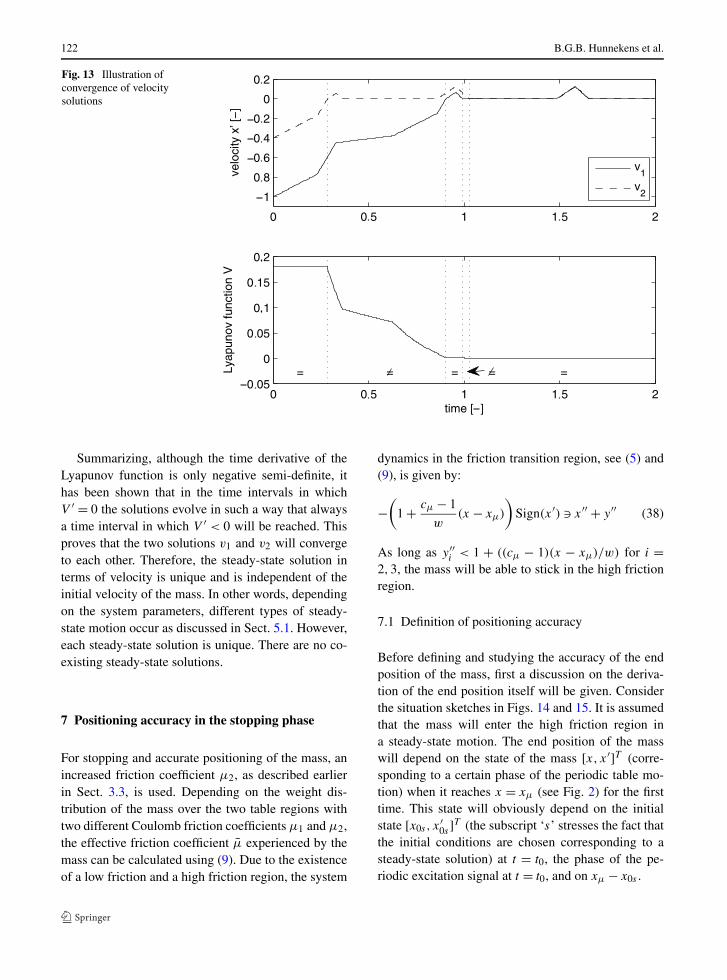
7.1 Definition of positioning accuracy
Before defining and studying the accuracy of the endposition of the mass, first a discussion on the deriva-tion of the end position itself will be given. Considerthe situation sketches in Figs. 14 and 15. It is assumedthat the mass will enter the high friction region ina steady-state motion. The end position of the masswill depend on the state of the mass [x, x′]T (corre-sponding to a certain phase of the periodic table mo-tion) when it reaches x = xμ (see Fig. 2) for the firsttime. This state will obviously depend on the initialstate [x0s , x
′0s]T (the subscript ‘s’ stresses the fact that
the initial conditions are chosen corresponding to asteady-state solution) at t = t0, the phase of the pe-riodic excitation signal at t = t0, and on xμ − x0s .
Vibrational self-alignment of a rigid object exploiting friction 123
Fig. 14 Situation sketch of when the mass is stopped
Fig. 15 Region of end positions where the mass can stop
The position where the mass stops, is defined byxμ + �xovershoot. The effective displacement in thelow friction region, during one excitation period insteady state, can be written as v�t (v is the averagevelocity during one excitation period). The maximumdisplacement in one period is defined as �x. To in-clude all possible ways of entering the high frictionregion in steady state, define xμ = �x and vary theinitial positions corresponding to steady-state x0s inthe range −v�t ≤ x0s ≤ 0. Corresponding initial ve-locities x′
0s are used to assure steady-state motion fromthe start. Now, collecting all overshoots �xovershoot ∈[�xovershoot,min, �xovershoot,max] for all initial con-ditions corresponding to steady-state responses, willprovide a range of the possible end positions of themass. The positioning error is now defined as:
�xd = �xovershoot,max − �xovershoot,min
2(39)
The desired end position can now be defined asxd = xμ + �xovershoot,min + �xd , see Fig. 15.
7.2 Results
The positioning accuracy will, next to system prop-erties, obviously depend on the prescribed table mo-tion. In Sect. 5, the stroke and frequency of the ta-ble were fixed and the accelerations y′′
2 and y′′3 were
varied. For different combinations of y′′2 and y′′
3 , thepositioning error is calculated and stored. In this sec-tion and in Sect. 7.3, the stroke and the excitation pe-riod of the table are set to respectively �y = 0.084and �t = 1. The dimensionless width is chosen tobe w = 0.05. It is assumed that cμ = 2.5 such thatthe friction coefficient in the high friction region isμ2 = 2.5μ. Hence, the interesting region of acceler-ations is limited to y′′
i < 1 + (cμ − 1)(x − xμ)/w, soto accelerations y′′
i < 2.5 (enabling the mass to per-manently stick to the table). Remarkably, as will beshown below, a design space for y′′
2 and y′′3 can be
identified where the positioning error is �xd = 0.Consider the following two table acceleration set-
tings: (y′′2 , y′′
3 ) = (2.3,1.3) and (y′′2 , y′′
3 ) = (1.8,1.1).In Fig. 16, the two corresponding phase portraits areshown. For each setting, two responses correspond-ing to two different initial conditions are shown. Thetwo dashed vertical lines respectively indicate the po-sitions, where the high friction region is starting (xμ),and from where it is possible for the mass to perma-nently stick to the table (xstick,min). The position onthe table, from where the mass is able to permanentlystick to the table, is determined by the following con-dition:
max(y′′i ) = 1 + cμ − 1
w(x − xμ) (40)
Using this condition, the position xstick,min can be cal-culated to be:
xstick,min = xμ + wmax(y′′
i ) − 1
cμ − 1(41)
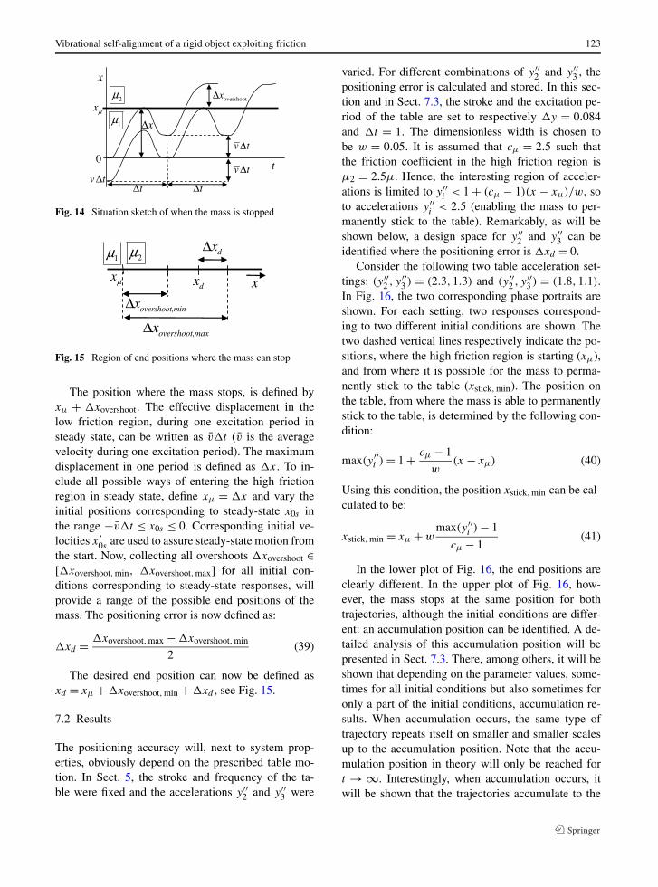
In the lower plot of Fig. 16, the end positions areclearly different. In the upper plot of Fig. 16, how-ever, the mass stops at the same position for bothtrajectories, although the initial conditions are differ-ent: an accumulation position can be identified. A de-tailed analysis of this accumulation position will bepresented in Sect. 7.3. There, among others, it will beshown that depending on the parameter values, some-times for all initial conditions but also sometimes foronly a part of the initial conditions, accumulation re-sults. When accumulation occurs, the same type oftrajectory repeats itself on smaller and smaller scalesup to the accumulation position. Note that the accu-mulation position in theory will only be reached fort → ∞. Interestingly, when accumulation occurs, itwill be shown that the trajectories accumulate to the
124 B.G.B. Hunnekens et al.
Fig. 16 Phase portraits oftwo different settings whenstopping the mass
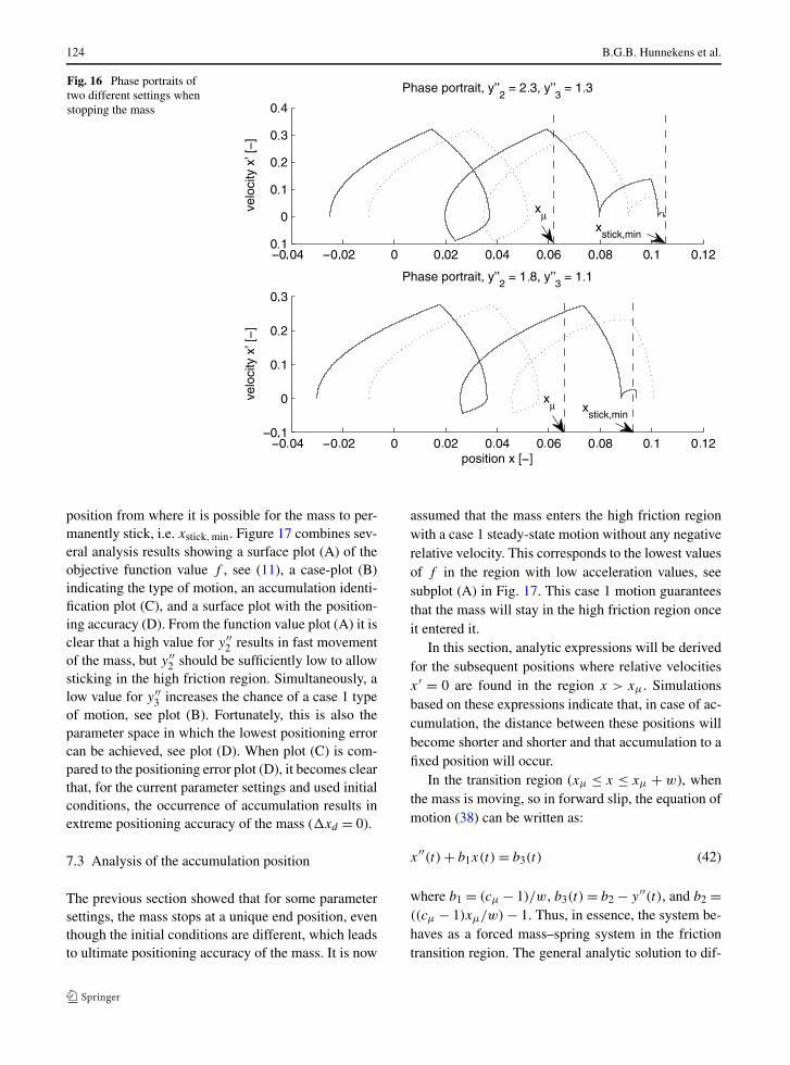
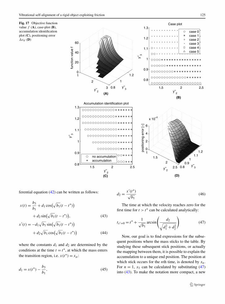
position from where it is possible for the mass to per-manently stick, i.e. xstick,min. Figure 17 combines sev-eral analysis results showing a surface plot (A) of theobjective function value f , see (11), a case-plot (B)indicating the type of motion, an accumulation identi-fication plot (C), and a surface plot with the position-ing accuracy (D). From the function value plot (A) it isclear that a high value for y′′
2 results in fast movementof the mass, but y′′
2 should be sufficiently low to allowsticking in the high friction region. Simultaneously, alow value for y′′
3 increases the chance of a case 1 typeof motion, see plot (B). Fortunately, this is also theparameter space in which the lowest positioning errorcan be achieved, see plot (D). When plot (C) is com-pared to the positioning error plot (D), it becomes clearthat, for the current parameter settings and used initialconditions, the occurrence of accumulation results inextreme positioning accuracy of the mass (�xd = 0).
7.3 Analysis of the accumulation position
The previous section showed that for some parametersettings, the mass stops at a unique end position, eventhough the initial conditions are different, which leadsto ultimate positioning accuracy of the mass. It is now
assumed that the mass enters the high friction regionwith a case 1 steady-state motion without any negativerelative velocity. This corresponds to the lowest valuesof f in the region with low acceleration values, seesubplot (A) in Fig. 17. This case 1 motion guaranteesthat the mass will stay in the high friction region onceit entered it.
In this section, analytic expressions will be derivedfor the subsequent positions where relative velocitiesx′ = 0 are found in the region x > xμ. Simulationsbased on these expressions indicate that, in case of ac-cumulation, the distance between these positions willbecome shorter and shorter and that accumulation to afixed position will occur.
In the transition region (xμ ≤ x ≤ xμ + w), whenthe mass is moving, so in forward slip, the equation ofmotion (38) can be written as:
x′′(t) + b1x(t) = b3(t) (42)
where b1 = (cμ − 1)/w, b3(t) = b2 − y′′(t), and b2 =((cμ − 1)xμ/w) − 1. Thus, in essence, the system be-haves as a forced mass–spring system in the frictiontransition region. The general analytic solution to dif-
Vibrational self-alignment of a rigid object exploiting friction 125
Fig. 17 Objective functionvalue f (A), case-plot (B),accumulation identificationplot (C), positioning error�xd (D)
ferential equation (42) can be written as follows:
x(t) = b3
b1+ d1 cos
(√b1(t − t∗)
)
+ d2 sin(√
b1(t − t∗)), (43)
x′(t) = −d1
√b1 sin
(√b1(t − t∗)
)
+ d2
√b1 cos
(√b1(t − t∗)
)(44)
where the constants d1 and d2 are determined by theconditions at the time t = t∗, at which the mass entersthe transition region, i.e. x(t∗) = xμ:
d1 = x(t∗) − b3
b1, (45)
d2 = x′(t∗)√b1
(46)
The time at which the velocity reaches zero for thefirst time for t > t∗ can be calculated analytically:
tx′=0 = t∗ + 1√b1
arcsin
(d2
√
d21 + d2
2
)
(47)
Now, our goal is to find expressions for the subse-quent positions where the mass sticks to the table. Bystudying these subsequent stick positions, or actuallythe mapping between them, it is possible to explain theaccumulation to a unique end position. The position atwhich stick occurs for the nth time, is denoted by xn.For n = 1, x1 can be calculated by substituting (47)into (43). To make the notation more compact, a new
126 B.G.B. Hunnekens et al.
time scale τ is introduced, which is zero at the mo-ment when the mass gets out of the first stick phasein the transition region. The mass will stick at the y′′
3part of the trajectory. The mass therefore starts to slipat τ = 0 when the acceleration changes from y′′
1 = 0to −y′′
2 . The following values apply at τ = 0:
b3,1 = b2 + y′′2 , (48)
d1,1 = xn − b3,1
b1, (49)
d2,1 = 0√b1
= 0 (50)
Note that b1 and b2 are constant in the transition re-gion. The first part of the analytic solution for 0 ≤ τ ≤t2 − t1 can therefore be written as follows:
x(τ) = b3,1
b1+ d1,1 cos
(√b1τ
), (51)
x′(τ ) = −d1,1
√b1 sin
(√b1τ
)(52)
At τ = t2 − t1, the acceleration changes from −y′′2
to y′′3 . At τ = t2 − t1, the following values apply:
b3,2 = b2 − y′′3 , (53)
d1,2 = x(t2 − t1) − b3,1
b1, (54)
d2,2 = x′(t2 − t1)√b1
(55)
which yields the following analytic solution for timeinterval t2 − t1 ≤ τ ≤ τx′=0, where τx′=0 is the time atwhich the relative velocity x′ becomes zero again:
x(τ) = b3,2
b1+ d1,2 cos
(√b1(τ − (t2 − t1))
)
+ d2,2 sin(√
b1(τ − (t2 − t1)))
(56)
x′(τ ) = −d1,2
√b1 sin
(√b1(τ − (t2 − t1))
)
+ d2,2
√b1 cos
(√b1(τ − (t2 − t1))
)(57)
Using (47), the mass gets into stick in the transitionregion for the second time, at time:
τx′=0 = (t2 − t1) + 1√b1
arcsin
(d2,2
√d2
1,2 + d22,2
)
(58)
The displacement at τx′=0 will be denoted byxn+1 = x(τx′=0). After algebraic manipulation the fol-lowing mapping between subsequent positions xn andxn+1 can be found:
xn+1 = b2 − y′′3
b1
+{(
y′′2 + y′′
3
b1+
(
xn − b2 + y′′2
b1
)
× cos(√
b1(t2 − t1)))2
+((
xn − b2 + y′′2
b1
)
sin(√
b1(t2 − t1)))2
} 12
(59)
The fixed point of this mapping can be calculated:
xn = xn+1 = b2 + y′′2
b1= xstick,min (60)
Recall that b1 = (cμ − 1)/w and b2 = (cμ − 1)xμ/
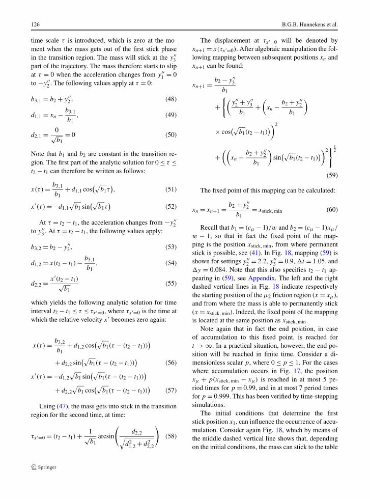
w − 1, so that in fact the fixed point of the map-ping is the position xstick,min, from where permanentstick is possible, see (41). In Fig. 18, mapping (59) isshown for settings y′′
2 = 2.2, y′′3 = 0.9, �t = 1.05, and
�y = 0.084. Note that this also specifies t2 − t1 ap-pearing in (59), see Appendix. The left and the rightdashed vertical lines in Fig. 18 indicate respectivelythe starting position of the μ2 friction region (x = xμ),and from where the mass is able to permanently stick(x = xstick,min). Indeed, the fixed point of the mappingis located at the same position as xstick,min.
Note again that in fact the end position, in caseof accumulation to this fixed point, is reached fort → ∞. In a practical situation, however, the end po-sition will be reached in finite time. Consider a di-mensionless scalar p, where 0 ≤ p ≤ 1. For the caseswhere accumulation occurs in Fig. 17, the positionxμ + p(xstick,min − xμ) is reached in at most 5 pe-riod times for p = 0.99, and in at most 7 period timesfor p = 0.999. This has been verified by time-steppingsimulations.
The initial conditions that determine the firststick position x1, can influence the occurrence of accu-mulation. Consider again Fig. 18, which by means ofthe middle dashed vertical line shows that, dependingon the initial conditions, the mass can stick to the table
Vibrational self-alignment of a rigid object exploiting friction 127
Fig. 18 Depending on theinitial conditions,accumulation to a fixed endposition is possible
at a position x > xstick,min, or can exhibit the accumu-lating behavior and end up at x = xstick,min. Note thataccumulation to an end position will always occur ifxn+1(xμ) < xstick,min, and is then independent of theinitial conditions.
8 Conclusions and recommendations
In this paper, one-dimensional self-alignment of amass via stick-slip vibrations has been studied. Us-ing a suitable periodic table trajectory, it is possibleto move the mass into a desired direction and using anincrease in the friction coefficient it is possible to stopthe mass at a certain end position.
The first objective of this paper has been to designa trajectory for the table, such that the mass moves toa desired end position in the least possible amount oftime, given some table motion constraints. The designof a table motion profile, consisting of three time in-tervals with different constant accelerations has beendiscussed. For the mass, analytic steady-state solutionshave been derived, and a classification of the types ofsteady-state responses of the mass has been given.
Using Floquet theory for discontinuous systems,the local stability of the solutions has been proven.Due to the freedom in position, one Floquet multiplierwill always be equal to one. Furthermore, using a Lya-punov analysis, convergence of the velocity response
has been proven. In other words, different velocity so-lutions will converge to each other, independent of theinitial velocities. This convergence implies uniquenessof the velocity response of the mass.
The second objective of this paper has been tostop the mass at a desired end position with the bestpossible positioning accuracy. For certain parametersettings, an interesting phenomenon is observed inthe transition region from low friction to high fric-tion, namely accumulation of the mass position to aunique end position. This accumulation behavior ben-efits the positioning accuracy in an ultimate manner. Inessence, the system behaves as a forced mass–springsystem in this region, which allows for an analyticalstudy of the accumulation behavior. Subsequent stick-positions have been related to each other resulting ina discrete mapping. It is shown that the fixed point ofthis mapping is exactly the position from where per-manent stick becomes possible. Under certain condi-tions, accumulation will always occur, independent ofthe initial conditions.
Recommendations for future research are: (1) ex-perimental verification of the analyzed behavior;(2) analysis of models with resembling, but more re-alistic, table motion profiles, i.e. finite values for thejerk should be introduced at times when the table ac-celeration values change; (3) use of enhanced frictionmodels; (4) extension to two-dimensional models de-
128 B.G.B. Hunnekens et al.
scribing general planar motion of the mass; and (5)extension to self-alignment of multiple masses.
Open Access This article is distributed under the terms of theCreative Commons Attribution Noncommercial License whichpermits any noncommercial use, distribution, and reproductionin any medium, provided the original author(s) and source arecredited.
Appendix: Details of the prescribed table motiongeneration using three acceleration parts
In order to calculate a table trajectory that satisfies the7 constraints formulated in Sect. 4.4.3, it is necessaryto find explicit expressions for the following 5 vari-ables: t1, t2, t3, yini, and y′
ini. Note that the followingtwo variables are already explicitly known: y′′
1 = 0 andt0 = 0. It is therefore only needed to solve 5 constraintequations, which can be derived from the constraintsformulated in Sect. 4.4.3. Using Fig. 7 the following5 equations can be derived:
1. yini = 1
2y′′
3 (t3 − ty′=0,2)2 (61)
2. t3 − t0 = �t (62)
3.1
2y′′
2 (t2 − ty′=0,1)2 + 1
2y′′
3 (ty′=0,2 − t2)2 = �y (63)
4.
y′ini(t1 − t0) + 1
2y′′
2 (ty′=0,1 − t1)2
+ 1
2y′′
3 (t3 − ty′=0,2)2
= 1
2y′′
2 (t2 − ty′=0,1)2 + 1
2y′′
3 (ty′=0,2 − t2)2
(64)
5. y′′3 (t3 − t2) = y′′
2 (t2 − t1) (65)
For convenience, in these equations two additionalunknowns are introduced, namely ty′=0,1 and ty′=0,2,which are the times at which the velocity y′ of the ta-ble becomes zero. Therefore, to solve the set of equa-tions, two additional equations are needed, which de-fine these two additional unknowns:
6. y′ini − y′′
2 (ty′=0,1 − t1) = 0 (66)7. y′
ini − y′′3 (t3 − ty′=0,2) = 0 (67)
Now 7 equations are available in the 7 unknownst1, t2, t3, yini, y′
ini, ty′=0,1, and ty′=0,2. This set of equa-tions is solved by the symbolic toolbox of Matlab. The
explicit solutions are not given here because the ex-pressions are too long to display.
Please note that actually there is a second case thatneeds to be considered. If the initial velocity y′
ini ap-pears to be smaller than 0, then the previously dis-cussed mathematical description of the constraints isnot valid anymore. However, a completely equivalentreasoning as for the case y′
ini > 0 can be followed.Therefore, the second case is not discussed in detailhere. Moreover, note that it is possible that no physi-cal solutions exist for the above specified equations if,for example, a large displacement �y is demanded ina short amount of time �t , using small accelerationvalues y′′
2 and y′′3 . In that case the solutions of some
variables will be complex valued, lacking a physicalinterpretation.
Acknowledgements This work was supported in part by agrant from Miami University’s School of Engineering and Ap-plied Sciences for International collaborations.
References
1. Armstrong-Hélouvry, B., Dupont, P., Canudas De Wit, C.:A survey of models, analysis tools and compensation meth-ods for the control of machines with friction. Automatica30(7), 1083–1138 (1994)
2. Berger, E.J.: Friction modeling for dynamic system simu-lation. Appl. Mech. Rev. 55(6), 535–577 (2002)
3. Blekhman, I.I.: Vibrational Mechanics—Nonlinear Dy-namic Effects, General Approach, Applications. World Sci-entific, Singapore (2000)
4. Chernous’ko, F.L.: Analysis and optimization of the motionof a body controlled by means of a movable internal mass.PMM J. Appl. Math. Mech. 70, 819–842 (2006)
5. Dankowicz, H., Normark, A.B.: On the origin and bifur-cations of stick-slip oscillations. Physica D 136, 280–302(2000)
6. Den Hartog, J.P.: Forced vibrations with combinedCoulomb and viscous damping. ASME J. Appl. Mech. 53,107–115 (1930)
7. Duarte, F.B., Machado, J.T.: Fractional describing functionof systems with Coulomb friction. Nonlinear Dyn. 56, 381–387 (2009)
8. Fidlin, A., Thomsen, J.J.: Predicting vibration-induced dis-placement for a resonant friction slider. Eur. J. Mech. Solids20, 807–831 (2001)
9. Frutiger, D.R., Vollmers, K., Kratochvil, B., Nelson, B.J.:Small, fast, and under control: wireless resonant magneticmicro-agents. Exp. Robot. 54, 169–178 (2009)
10. Galvanetto, U., Bishop, S.R.: Dynamics of a simpledamped oscillator undergoing stick-slip vibrations. Mecca-nica 34, 337–347 (1999)
11. Leine, R.I., Nijmeijer, H.: Dynamics and Bifurcationsof Non-Smooth Mechanical Systems. LNACM, vol. 18.Springer, Berlin (2004)
Vibrational self-alignment of a rigid object exploiting friction 129
12. Leine, R.I., van de Wouw, N.: Stability and Convergence ofMechanical Systems with Unilateral Constraints. LNACM,vol. 36. Springer, Berlin, Heidelberg, New-York (2008)
13. Luo, A.C.J., Gegg, B.C.: Stick and non-stick periodic mo-tions in periodically forced oscillators with dry friction.J. Sound Vib. 291, 132–168 (2006)
14. Moreau, J.J.: Unilateral contacts and dry friction in finitefreedom dynamics. Non-Smooth Mech. Appl., 302 (1988)
15. Natsiavas, S.: Stability of piecewise linear oscillators withviscous and dry friction damping. J. Sound Vib. 217(3),507–522 (1998)
16. Pogromsky, A.Yu., Heemels, W.P.M.H., Nijmeijer, H.: Onsolution concepts and well-posedness of linear relay sys-tems. Automatica 39, 2139–2147 (2003)
17. Rakotondrabe, M., Haddab, Y., Lutz, P.: Development,modeling, and control of a micro-/nanopositioning 2-dofstick-slip device. IEEE/ASME Trans. Mechatron. 14(6),733–745 (2009)
18. Reznik, D.S., Canny, J.F., Alldrin, N.: Leaving on a planejet. In: IEEE International Conference on Intelligent Robotsand Systems, Maui, HI, pp. 202–207, October (2001)
19. Sato, K., Ito, K., Hata, S., Shimokohbe, A.: Self-alignmentof microparts using liquid surface tension—behavior of mi-cropart and alignment characteristics. Precis. Eng. 27, 42–50 (2003)
20. Shaw, S.W.: On the dynamical response of a system withdry friction. J. Sound Vib. 108(2), 302–325 (1986)
21. Stein, G.J., Zahoransky, R.: On dry friction modelling andsimulation in kinematically excited oscillatory systems.J. Sound Vib. 311, 74–96 (2008)
22. Studer, C.: Numerics of Unilateral Contacts and Friction—Modeling and Numerical Time Integration in Non-SmoothDynamics. LNACM, vol. 47. Springer, Berlin, Heidelberg(2009)
23. Thomsen, J.J.: Some general effects of strong high-frequency excitation: stiffening, biasing, and smoothening.J. Sound Vib. 253, 807–831 (2002)
24. Thomsen, J.J., Fidlin, A.: Analytical approximations forstick-slip vibration amplitudes. Int. J. Non-Linear Mech.38, 389–403 (2003)