Viability of Weather Index Insurance

in Managing Drought Risk in Australia

Prepared by Adeyinka, A.A., Krishnamurti, C., Maraseni, T and

Chantarat, S.

Presented to the Actuaries Institute

Actuaries Summit

20-21 May 2013

Sydney

This paper has been prepared for Actuaries Institute 2013 Actuaries Summit.

The Institute Council wishes it to be understood that opinions put forward herein are not necessarily those of

the Institute and the Council is not responsible for those opinions.

< Adeyinka, A.A., Krishnamurti, C., Maraseni, T. Chantarat, S >

The Institute will ensure that all reproductions of the paper

acknowledge the Author/s as the author/s, and include the above

copyright statement.

Institute of Actuaries of Australia

ABN 69 000 423 656

Level 7, 4 Martin Place, Sydney NSW Australia 2000

t +61 (0) 2 9233 3466 f +61 (0) 2 9233 3446

e actuaries@actuaries.asn.au w www.actuaries.asn.au

ii

Abstract

In this paper, we look into the risk management strategies adopted by

farmers to manage revenue shortfall resulting from drought-induced

yield losses. We survey literature on traditional indemnity–based

insurance and weather index insurance. Some challenges facing the

indemnity-based insurance were discussed and the prospects of

resolving these challenges by using an index based risk transfer product

called weather index insurance was analysed. The particular weather

variable of interest was rainfall. Basis risk and methodological

challenges were recognized as some of the major challenges to the

uptake of weather index insurance. We showed the relationship

between yield and cumulative precipitation indices using regression

analyses. The hedging efficiency of the product was analysed using

the Mean Root Square Loss (MRSL) and Conditional Tail Expectation

(CTE) while the systemic nature of the risk was captured with Loss

Ratios. We concluded that a strong relationship between the rainfall

index and yield does not necessarily lead to high hedging efficiency

and other variables would have to be taken into consideration in order

to make the design of weather index insurance more robust. We found

that the MRSL is more resistant to strike levels of the contracts than the

CTE. The results from the Loss Ratio Analysis showed that spatial and

temporal pooling of insurance contracts reduce the risk to the insurer.

Keywords: Weather index insurance, hedging efficiency, burns analysis,

conditional tail expectations, mean root square loss, loss ratio, quantile

regression analysis, drought.

Please, refer to these abbreviations for quick reference although they

are explicit within the text CSPI - Cumulative Standardized Precipitation Index PReg – Panel Data Regression Analysis

CTE – Conditional Tail Expectation QLD - Queensland

CV – Coefficient of Variation QReg – Quantile Regression

FE – Fixed Effect RE – Random Effect

LR – Loss Ratio SD – Standard Deviation

MRSL – Mean Root Square Loss SPI – Standardized Precipitation Index

OReg – Ordinary Least Square Regression WA – Western Australia

iii

Table of contents page

1. Introduction............................................................................................. 1

2. Weather and Climate Risk Management in Australian Agriculture. 2

3. Weather Index Insurance versus Traditional Insurance ........................5

4. Legal Treatment of Weather Derivatives and Insurance.....................6

5. Weather Index Insurance and Climate Change .................................8

6. Global Experience in the use of Weather Index Insurance ................9

7. Methodological framework...................................................................10

8. Summary of Results.................................................................................14

9. Discussion.................................................................................................26

10. Conclusions and Recommendations...................................................28

References ...................................................................................................29

Appendices ..................................................................................................35

NOTE: Neither the authors nor the institute of actuary of Australia would

indemnify any individual or entity should any part of this report be used

to inform any decision that warrants indemnification.

1

1. 1 Introduction

The insurance system is getting over stretched given the frequency and intensity of

extreme weather events in recent years (Keenan & Cleugh 2011; Parry et al. 2007).

Although, extreme weather events like drought affect most sectors in the economy at

least indirectly, some sectors are more vulnerable than others. The agricultural sector

is among those sectors most vulnerable because rainfall deficit has grave implications

on dry land crop yields and livestock grazing (Bardsley, Abey & Davenport 1984;

Chantarat et al. 2007; Ghiulnara & Viegas 2010; Kimura & Antón 2011). Previous

efforts to insure against the covariate nature of drought risk have been considered

inefficient (Miranda & Glauber 1997).

Recently, Kimura and Antón (2011) recommended the exploration of insurance

markets to manage drought risk in Australia. This suggestion by Kimura and Antón

(2011) is in tandem with that of Bardsley (1986) that the viability of rainfall insurance

is contingent on the relationship between yield losses and the index used as proxy for

payout for the insurance contracts and the behaviour of a portfolio of the contracts

when aggregated over time and space. The case of weather index insurance is

different from certain existing insurance contracts like household fire insurance in that

drought risk is usually systemic and therefore less diversifiable.

Literature on the use of weather index insurance as a means of hedging climate related

risk is growing, but there has been a focus on temperature related risks in the energy

industry without much consideration given to rainfall insurance as a means of hedging

shortfalls in agricultural productions (Bokusheva 2011; Sharma & Vashishtha 2007;

Vedenov & Barnett 2004; Yang, Brockett & Wen 2009). Researchers have related

crop yields to weather indices but concluded that there is need for an in-depth analysis

of crop and region specific studies (Bardsley, Abey & Davenport 1984; Turvey 2001;

Vedenov and Barnett 2004). This region-specific analysis of rainfall insurance

focusing on wheat was conducted by Bardsley, Abey and Davenport (1984) for some

shires in New South Wales (NSW) in Australia, however, the data used was from

1945 to 1969 and interstate risk pooling was not modelled. Although the authors

agreed that pooling risk beyond NSW will lower the risk to the insurer. Given that the

data covered only a 25 year period and the climatic realities observed within the

period may be different from what obtains at the moment in light of climate change,

there is need for a re-examination of the topic with a longer and more recent data.

The conclusions in Bardsley (1986) suggest that weather index insurance is a possible

tool for managing drought risk but Binswanger-Mkhize (2012) is of the view that

there is too much hype about weather index insurance. The major challenge facing the

prospects of weather hedging in the agricultural sector is the empirical estimation of

2

necessary parameters involved including prices and the dependence structure of the

risk among others (Jewson & Brix 2005).

The general objective of this study was to determine the viability of weather index

insurance. More specifically, we determined the relationship between weather index

and yield. Also, the hedging efficiency of weather index insurance was determined

and finally, we determined the extent to which a portfolio of weather index insurance

is diversifiable. We discussed the literature surrounding weather index insurance and

the methodology adopted after which the analysis follows the sequence of the specific

objectives. The paper ended with discussion of the findings and conclusion.

2. Weather and Climate Risk Management in Australian Agriculture

The Australian agricultural system is susceptible to extreme weather particularly

drought risk that has become an integral part of the system. This has lead to a

paradigmatic shift in the perception of drought as a disaster to a risk that requires self-

sufficiency on the part of the farmer as stated in the Australian Drought Policy (Kokic

et al. 2007; Lindesay 2005; Wilhite 2005). Consequently, there is a re-assessment of

the role of weather index insurance in the context of agricultural risk management

particularly in Australia given its susceptibility to drought. This susceptibility and the

consequent paradigm shift have lead to a re-examination of the role of weather index

insurance in Australian agriculture as noted in Kimura and Anton (2011) although the

debate on its viability remains inconclusive as observed in the work of Quiggin

(1994):

While the debate did not reach a settled conclusion, there was a consensus

that a rainfall insurance scheme would not have a major impact in the

absence of some subsidy at least on administrative costs. On the other hand, if

subsidies were to be paid to farmers suffering from adverse climatic

conditions, rainfall insurance would be one of the most cost-effective

alternatives. (p. 123).

Nevertheless, Quiggin (1986) are of the view that we can achieve reduction in the cost

of risk if government’s policies do not deter the design of insurance schemes.

Similarly, Zeuli and Skees (2005) opined that some benefits may be possible with

weather index insurance and that as little as the benefits may be, it could mean much

to farmers who are exposed and have no other cover.

Weather risk, like every other risk, involves the probability and intensity of loss

(Bodie & Merton 1998; Cuevas 2011). The economists’ position is that risk is the

variance in the outcome that results from an action. This economist’s view is implied

in Adam Smith’s perception of insurance as a trade that gives security to individuals

3

in that these individuals could trade their risks for a portion of their utility (Zweifel &

Eisen 2012, p. v). This trade is primarily a trade-off between the expectation of the

outcome and its variance (Hayman & Cox 2005, p. 119). The etymological history of

risk emphasises choice and opportunities rather than loss and fate and the ability to

manage variability remains a major source of entrepreneurial competitiveness

(Bernstein 1996). Managing risks therefore involves making choices among a range

of competing alternatives through adequate consideration of costs and benefits

(Harwood et al 1999). There are several sources of risk in agriculture including

drought and given that weather could no longer be treated as a force majeure, hedging

it has become an issue of paramount importance (Kimura & Antón 2011).

Enterprise diversification, crop insurance and government welfare supports are among

alternatives that have been traditionally available to farmers to manage revenue

fluctuations resulting from the impacts of exogenous variables on yield (Harwood et

al. 1999). There are three layers of risk as noted in OECD work on risk management

in agriculture (OECD 2011). The first layer is normal risk which is frequent but not

too damaging. At the intermediate layer is the marketable risk which is more frequent

but more damaging but not to a catastrophic extent. The third layer is catastrophic risk

which is least frequent but most destructive. Generally, enterprise diversification is

useful in managing the first layer of risk in that though the probability of occurrence

of risk at this level is high; its impact is very low. At the second layer, the frequency

of the risk is lower than the first but has a higher impact while the third layer has the

lowest frequency but maximum impact because of its systemic nature. The second

layer could be readily managed using market-based instruments to promote self-

reliance. This layer of risk coincides with the level of risk that farmers are willing to

insure unlike events that have low probability with more disastrous consequences

which are hardly given considerations in risk planning (Wright & Hewitt 1994).

Given the covariate nature of drought risk at the extreme tail, drought may be

uninsurable in the domestic market and governments have often acted as risk bearer

of last resort (O’Meagher 2005; Quiggin, Karagiannis & Stanton 1994). Reinsurance

has been suggested as an alternative to manage the covariance of drought risk at the

extreme tail in that pooling the risk in a larger portfolio of risk makes it bearable for

the reinsurer unlike a local insurance firm (Chantarat 2009). The reinsurer has the

capacity to pool the risk over space and risk pooling over time could also provide

additional diversification opportunities (Hoeppe & Gurenko 2006). This alternative

makes response swift and takes the declaration of exceptional circumstances beyond

political advocacy that has characterised government response in Australia and other

parts of the world (Kimura & Antón 2011).

Besides drought relief, governments have traditionally used multi-peril crop insurance

to manage drought risk but the work of Wright and Hewitt (1994) described the

objective function of multi-peril crop insurance and its basic assumptions as untenable

4

(p. 85). They noted that the main reason for the failure of all-risk insurance was that it

is based on a theoretical model that overstates its potential value. Drought relief is one

method the government uses to assist farmers and is not without its own criticism as

well (Meuwissen, Van Asseldonk & Huirne 2008). The major argument is that

drought assistance is subjective and politicised besides the equity issues it raises

(Kimura & Antón 2011). Drought is considered as a part of agricultural endeavours

especially in a country like Australia and government intervention has been left to

exceptional circumstances the declaration of which is flawed (Keenan & Cleugh

2011; Kimura & Antón 2011; Meuwissen, Van Asseldonk & Huirne 2008; Quiggin

1994). The work of (Botterill & Wilhite 2005) shows that farmers are expected to

manage the first and second layer of drought risk but they are yet to be empowered

with the necessary mechanism to manage the second layer. The third layer of risk has

been called an exceptional circumstance but its benchmarking as a once in 20 to 25

year event is questionable given recent trends in the frequency of drought (Kimura &

Antón 2011). The once in 20 year drought corresponds to the Bureau of

Meteorology’s 5th

percentile rainfall (BoM 2012). Since the multi-peril crop insurance

is highly cost prohibitive given its loss ratios (Quiggin 1994; Wright & Hewitt 1994)

and governments’ efforts are subjective, Index Based Risk Transfer Products

(IBRTPs) have been considered as useful alternatives to managing agricultural

production risks (Kimura & Antón 2011). A particular type of IBRTP is weather

index insurance, an agro-insurance to prevent risk avoidance on the part of farmers.

Recent experiences have shown that without significant subsidies, the agro-insurance

market will be thin (Smith & Glauber 2012). However, Skees and Collier (2012)

found that premium subsidies can undermine the essence of weather market. Helping

farmers to manage their risks curtails risk avoidance that could culminate in the

redeployment of factors of production invested in agriculture. Hence, the government

of Australia has taken several initiatives to assist farmers but these initiatives are not

without their accompanying inefficiencies particularly slow response, politicization

and inequity (Kimura & Anton 2011).

Generally, public agencies tend to be associated with inefficiencies and a private

alternative is often considered as the solution which unfortunately is not always the

case (Niskanen 1971). Subsidizing the contracts and outsourcing it to private firms

could lead to rent seeking behaviours, besides, Smith and Glauber (1971) are of the

view that insurance subsidy is a form of wealth transfer to farmers. This wealth

transfer is an incentive for farmers to make sub-optimal decisions as few farmers are

willing to pay the full price of insurance. Therefore, if individuals expect

compensation, in whatever form, from government to offset natural disaster losses,

they will take on additional risks. If producers do not bear the consequences of risky

decisions, they will continue to do the things that expose them to the risk.

5

3. Weather Index Insurance and Traditional Indemnity-Based Insurance

Two major types of insurance products exist namely; traditional indemnity-based

insurance and index–based insurance. Under the traditional category are the named

peril, multiple peril and mutual insurance products. The index-based products include

yield and weather insurance. The payouts from traditional indemnity-based insurance

products are based on the actual losses farmers experienced whereas some proxies are

used as the basis for payouts under the index based products (Turvey 2001; Chantarat

2009).

The most commonly cited advantages of index-based insurance are that it prevents

moral hazards and adverse selections. Moral hazard is any behaviour of the insured

that makes him not to protect himself against losses in anticipation of indemnity

payment. Since, weather index insurance is based on exogenous variables beyond the

control of both counterparties to the insurance contracts the asymmetric information

leading to the problem of moral hazard plaguing the traditional indemnity insurance

will be resolved. The cost of monitoring moral hazards increases the cost of

traditional insurance. It is expected that index-based proxies like precipitation and

temperature would eliminate this cost thereby making weather index insurance

cheaper. However, the problem of basis risk reduces this cost benefit (Yang, Brockett

& Wen 2009).

Basis risk could be geographic or structural. Geographic basis risk creates a gap

between the station where the weather readings are made and the farm land insured.

Structural basis risk refers to creating weather index insurance that is not suited for

the particular crop. Using the currently traded precipitation derivatives used by the

energy industry will create structural basis risk for farmers in that the product is not

suitable for them. If the farm is located in Clifton, about 150 kilometres west of

Brisbane (Clifton 2012), then, there will be geographic basis risk if the weather

station in Brisbane is used for precipitation reading. To resolve the problem of basis

risk, the contracts may have to be localized thereby reducing the expected cost

savings of weather index insurance.

Adverse selection is also said to be characteristic of the traditional indemnity

insurance (Ahsan, Ali & Kurian 1982; Just, Calvin & Quiggin 1999). This is because

those who are the most affected by the peril of interest will tend to take the insurance

thereby creating a pool of risky contracts. Since the trade of insurance is supposed to

divide among a great many that loss which could ruin an individual (Adams Smith in

Zweifel & Eisen 2012, p.v), adverse selection makes this impossible as only those

individuals who are risky are in the insurer’s pool. If farmers are able to predict the

weather to a reasonable extent, then, adverse selection could still be possible with

weather index insurance in that farmers would only take cover in those years when

they are most at risk. Similarly, some locations could be at risk of droughts than the

6

others (Agnew 2011; Hicks 2011). The implication is that farmers who are farming in

locations at risk of drought will take drought insurance thereby creating a risky

portfolio of insurance contracts. The adverse selection resulting from this

geographical diversity could be aggravated if the pricing of the contracts does not

reflect the relative susceptibility of these locations to drought. Hence, if location A is

at higher risk than B, then the pricing should reflect this relative risk for the insured to

feel fairly treated. Hence the need for pareto-efficiency in the pricing of weather index

insurance contracts.

Since the insurance market operates like the capital market in that it enhances the

production capacity of farmers, it is better than non-market alternatives to managing

their risk exposures (Quiggin & Chambers 2004). The availability of these insurance

options raises some questions. These questions include; what insurance products are

most suitable to cater to the needs of primary producers and what are the legal

implications of these options?

4. Legal Treatment of Weather Derivatives and Insurance

Weather hedges could be purchased as derivatives or insurance and they have certain

similarities and differences (Raspe 2002; Skees & Collier 2012). In terms of

similarities, weather insurance and derivatives require the forfeiture of a premium to

be entitled to receive payouts should a contingent event occur. There are regulatory,

tax and accounting standard differences between the two products as noted by (Raspe

2002). The insurance market is highly regulated while derivatives are excluded from

too much regulatory scrutiny as long as it conforms to certain conditions (Raspe

2002).

In Kelly and Ball (1991), insurance contract was defined in the context of Australia

and it was noted that three essential requirements are needed for a contract to be an

insurance contract. The first is premium and benefit, the second being uncertainty of

the event and finally an interest besides that created by the insurance contract itself.

The premium paid obligates the insurer to confer value on the insured should the

fortuitous event occur as noted in Raspe (2002). Kelly and Ball (1991) argued that

these three requirements are also present in other contracts like warranties and

acknowledged the difficulties involved in defining insurance contract. Kimball-

Stanley (2008) identified two basic theories in articulating the difference between

insurance contracts and other contracts; they are legal interest test and the factual

expectancy test. Kelly and Ball (1991) recommended an approach that focuses on the

intention of the parties as being helpful. In particular, the intention of the assured who

has more information peculiar to the risk, to transfer possible losses to the insurer

confers on him (the assured) a duty of care in the form of disclosure of necessary

information. The duty of care by both parties in the risk assessment remains a major

distinguishing factor between insurance and other contracts.

7

Translating this definition into the context of weather hedging, we can say that since

meteorological information is publicly available, there is no private information to

disclose by the assured and the insurer has limited opportunities to engage in

malpractices. Premiums and benefits are evidently part of the contracts but the

uncertainty is not on whether or not drought will occur, rather, when it will occur.

Given recent advances in meteorological sciences, it may be possible to predict

occurrence of droughts to a reasonable degree of confidence. The implication is that

although weather information is publicly available, farmers may have enough

information to decide on when to purchase a cover in such a way to maximize their

own benefits at the expense of the insurer. The consequent adverse selection will lead

to weak temporal risk pooling as farmers will not take insurance in years they are

least likely to be drought stricken. Also, those in less drought prone areas will not take

insurance. The implication is that as insurers tend to factor in this form of adverse

selection into their pricing, the price of insurance will be driven upwards.

Following the thoughts of Raspe (2002, p. 225), ‘An entity executing a weather

derivative trade does not need to show an insurable interest. This interest is a major

distinguishing characteristic between insurance contract and a wager. An insurance

contract definition based on Section 1101(a)(1) of New York’s Insurance Laws given

in Raspe (2002, p. 226) is as follows:

[A]ny agreement or other transaction whereby one party, the “insurer”, is obligated

to confer benefit of pecuniary value upon another party, the “insured” or

“beneficiary”, dependent upon the happening of a fortuitous event in which the

insured or beneficiary has, or is expected to have at the time of such happening, a

material interest which will be adversely affected by the happening of such event.

The insured imposes the obligation to the insurer through the premium paid and the

occurrence of weather event remains one of the most fortuitous of all and therefore

helps to contain moral hazard which is typical of the traditional indemnity-based

insurance that requires proof of losses. However, the relationship between yield losses

and the weather index on which payout is based is not in absolute tandem with the

payout. This disparity results from structural and geographical basis risk characteristic

of weather index insurance. Hence, there could be years when there are losses without

payouts and years with payouts but no losses. At best, should all the years of payouts

match with years when losses are experienced, the payouts may not be commensurate

with the losses.

In essence, value is conferred on the insurer on the basis of the weather index but the

material insurable interest is the observed yield which translates into utility in the

form of revenue. The case of weather index insurance is similar to the amphibious

nature of preferred stock that stands between equity and debt with its unique legal

standards.

8

Recent studies seem to implicitly suggest that the structure of insurance contracts

follow the same structure as that of derivatives without any proof of loss but an

insurable interest exists (Chantarat 2009; Kapphan, Calanca & Holzkaemper 2012). It

seems that the function of weather index insurance may not be different from weather

derivatives but they require a well-articulated legal distinction to prevent abuse of the

classification and regulatory frameworks guiding derivatives and insurance. Failure to

regulate the products may create new risks (Kimball-Stanley 2008). Some authors

(Chantarat 2009; Kapphan 2012) in their reports interchangeably used insurance and

derivatives because of the functional convergence between the two products.

The possible mismatch in the payout and yield loss suggests that weather index

insurance may not completely satisfy the conditions of insurance like the traditional

indemnity-based insurance. Hence, in defining what constitutes insurance, there is

need to differentiate between indemnity-based insurance and index-based insurance.

A major similarity between the two insurance types is that they both require insurable

interests but there is no need for proof of loss in the case of index-based insurance.

The index-based insurance is also different from weather derivatives in that

derivatives do not necessarily require an insurable interest.

Skees and Collier (2012) noted that weather hedges could be purchased as over-the-

counter weather index products which are tailored to individual needs of the clientele

or as actively traded standardized exchange traded derivatives. Given the nature of the

response of different crops in different regions to weather variables, exchange traded

weather derivatives may not be practical in the context of agriculture because the

patronage for standardized contracts will be limited. Vortex (2012) effectively

summarized these differences in terms of eligibility to purchase the hedging product,

accounting treatment, liquidity, flexibility and regulatory control.

5. Weather Index Insurance and Climate Change

It is a well-established fact that weather variability is the major source of yield

fluctuations (Dai, Trenberth & Qian 2004; Kapphan, Calanca & Holzkaemper 2012)

and that weather variability will be exacerbated by Climate Change with a consequent

effect on yield (Keenan & Cleugh 2011). The old saying that; ‘however big floods get,

there will always be a bigger one coming ...’, is therefore true in relation to climate

change and drought (President’s water Comm. in Gumbel (1958). However, Kapphan,

Calanca and Holzkaemper (2011, p. 33) concluded that increase in weather risk,

particularly exacerbated by climate change, generates a huge potential for the

insurance industry. They showed that when hedging with contracts adjusted for future

climate scenarios, benefits almost triple for the insured while profits increase by

240% for the insurer. The implication is that weather index insurance would become

more profitable for both counterparties if it is updated to capture latest weather

9

information. In the study, it was further noted that insurers could suffer losses if future

contracts do not capture changes in weather distributions over the coming years.

Skees and Collier (2012) noted that the price of weather hedging will increase as

climate change increases weather risk. Consequently, the capacity of those at risk

could be impeded by the exorbitant prices that could prohibit the insured from taking

the insurance leading to insufficient demand. The low demand could have resulted in

economy of scale for the insurer offering the product. They noted that the price of the

insurance will increase for three reasons namely; increases in pure risk, the potential

size of losses and ambiguity of the risk. The link between climate change and the

price of weather insurance is due to the fact that the pricing is of the contract is done

using Historical Burns Analysis. Burns analysis involves the use of historical data to

estimate the fair premium of insurance. Hence, as there is a change in the data trend,

there will be a corresponding shift in the statistical parameters used in the estimation

of the prices. This model assumes that the insurer’s profit over the years is zero as the

premium is assumed to cover all indemnities only (Chantarat 2009; Jewson & Brix

2005; Kapphan, Calanca & Holzkaemper 2011).

6. Global Experience in the use of Weather Index Insurance

Weather index insurance has been successfully used in some countries while it is been

pilot tested in others and further researches are being undertaken in this area

(Gurenko 2006; Sharma & Vashishtha 2007). The case of Mongolia was emphasized

by Skees (2008) as a model for Low Income Countries (LICs). The Mongolian case is

a typical example of how index insurance could be used to hedge livestock losses.

The drought and harsh winter in the early 2000s in Mongolia lead to losses of about a

third of the country’s cattle. The disaster was financed through a loan agreement with

the World Bank to finance a tranche of index–based livestock insurance. In Honduras,

the use of weather index insurance has been found to be effective among smallholder

farmers (Nieto et al. 2012). The study by Bardsley, Abey and Davenport (1984)

focused on European agriculture. In the study, it was noted that perception of risk by

scientists and farmers are not necessarily in congruence and that a theoretically

promising risk management instrument may not necessarily work well for farmers.

This divergence in risk perception could partly explain the friction in the uptake of

weather index insurance by farmers. The study concluded that risk perception varies

considerably across EU member states. Another important conclusion of the study

was that risk management solutions need to be ‘tailor-made’ to cater to the diversity

in risk perception and exposure among the EU states.

10

7. Methodological framework

7.1: Data and data processing: The rainfall data used is based on the available data

from the Bureau of Meteorology of Australia (BoM 2012) and the yield data from the

Department of Primary Industry and Fisheries (Potgieter, Hammer & Doherty 2012).

The actual yield data is not available for a sufficiently reasonable period of time so

the simulated data was used. Although the simulated yield data is available from 1900

till 2011, the precipitation data is not sufficiently available over the same period in

many shires. Hence, a 40–year period was used from 1971 till 2010. There were

missing data in this period as well but experts were of the view that such missing data

are better taken as zero readings rather than using average values to substitute the

missing data.

There are different types of indices that could be used in the design of weather index

insurance (Chantarat et al. 2012; Dai, Trenberth & Qian 2004; Kapphan, Calanca &

Holzkaemper 2011; Turvey 2001). However, the Standardized Precipitation Index

(SPI) was used because it is relatively simplistic in comparison to the likes of Palmer

Drought Severity Index, Reconaissance Drought Index and others. The SPI is

calculated using the standardized values of rainfall. The season was divided into

dekads (ten day periods) and the SPI for each dekad was summed up to form the

Cumulative SPI (CSPI) which was used for benchmarking. The benchmarking was

done at percentile levels. For example, the 5th

percentile benchmark will imply that

the contracts will pay out twice in the 40–year period, the 10th percentile pays out

four years with the lowest SPI in the period while the 30th percentile pays out 12

years of the 40 years. The analysis was done with equal weightage of the dekads in

the season and then with optimized weightage. However, the emphasis was on the

optimized weightage because the optimized weights lead to a stronger relationship

between yield and the index. The equal weighting implies that each 10–day period in

the season equally influences crop yield whereas the optimized weightage implies that

some dekads have more impact than the others. The GRG nonlinear algorithm in

Microsoft Excel package was used to allocate weights that maximize the yield-index

relationship. In all cases the relationship was stronger when weights were optimized.

The commencement of the season for Queensland shires is around 1st of June while it

is approximately 1st of April in Western Australia, depending on the shire. The

periods covered by the contracts were from sowing to the commencement of maturity

over an approximately 180–day period from the commencement of the season. The

rainfall (in millimetres) was accumulated in dekads. We assumed a soil maximum

water retention capacity of 60mm for all the shires. This is because rainfall above this

amount may not contribute to plant growth (Stoppa & Hess 2003).

11

The following optimization problem was adopted to obtain the weights for the dekads:

Where ri* is the actual rainfall in period i, and CAPi is the amount of rainfall in the

particular dekad or period i above which additional rainfall will not increase wheat

yield.

Where n is the total number of 10-day periods in the growing season which in our

case is 18 ten-day periods, ωi, is the weight assigned to the period i of the growing

season, rit is the effective rainfall in period i of year t and = Cumulative

Standardized Precipitation Index for each year (t),

The weights, ωi, were chosen to maximize the sample correlation between the rainfall

index and yield based on the yield data from 1971 to 2010.

_ _2010

1971

1/2 1/2_ _

2010 20102 2

1971 1971

( )( )max ( , )

( ) ( )

;0 ,

t t

i

t t

cz cz z ztcz

cz cz z zt t

i i

R R Y Ycorr R Y

R R Y Y

Subject to the constraint

Where: Yt is the yield in year t, = average yield. These values vary from shire to

shire across both states.

7.2: Payout procedure: The contract design follows a put option design as described

in Turvey (2001), however, we follow the indemnity structure in Stoppa and Hess

(2003) for simplicity. The rainfall index derivative based on the Cumulative

Standardized Precipitation Index ( ) must be below an alpha (5th

, 10th and 30

th)

percentile threshold ( ) for payout to occur. The payment was designed to be

proportional to the extent to which the index is below the threshold. The value of

is the sum of the values obtained by multiplying the rainfall index in each period (i) of

a particular year (t) by the specific weight (ωi) assigned to the period i.

*max ,i i ir r CAP

t

n

cz i itiR r

12

0 if   

*

t

t

t

cz

cz

cz

R T

Indemnity LiabilityT RifR T

T

Where: tczR Cumulative Standardized Precipitation Index for each year t ;

percentile threshold,T th th th 5 , 10 and 30 percentiles 

The liability is the insurable interest or the value of a hectare of wheat which was

estimated using the average yield and the average monetary value of wheat. The price

is assumed to be the same for all shires because the national export price was used but

average yield differs from shire to shire. Hence, we are analysing the effect of

weather index insurance on the revenue of a representative wheat farmer in each shire

who took the average national price of $183.71 per hectare of wheat harvested (ABS

2012) over the 40-year period. Since the price is constant across the shires over the

period under consideration, our analyses basically focus on the effect of weather

derivatives or insurance on the hedgibility of the representative farmer’s revenue

resulting from the stochastic nature of wheat yield.

7.3: Data Analyses:

7.3.1: Objective 1: To determine the relationship between the weather index and

yield.

To achieve the first objective, the Ordinary Least Square Regression (OReg) was

adopted in an attempt to find the relationship between the weather index and yield.

However, since the OReg assumes uniform slope across the yield-index continuum,

the Quantile Regression (QReg) was utilized to study the strength of the relationship

at different quantiles on the continuum (Adeyinka & Kaino 2012; Koenker 2005) The

PReg (Panel Regression) analysis was used to determine the effect of location on the

analysis. In essence, we sought to know whether or not different indices are required

for different locations (Panel effect) (Chantarat 2009).

7.3.2: Objective 2: To determine the hedging efficiency of weather index insurance

The Standard Deviation (SD) may not be an appropriate measure of risk since we are

interested in the downside risk. Value at Risk (VaR) also has its short coming because

it is considered incoherent and does not satisfy the required axioms of an appropriate

risk measure (Acerbi & Tasche 2001). Therefore, the Conditional Tail Expectation

(CTE) and Mean Root Square Loss (MRSL), otherwise called Root Mean Square

Loss (RMSL), were used to measure the hedging efficiency of the insurance at

different strike levels (Vedenov & Barnett 2004). The CTE analysis in this study is

13

measured at the 5th, 10th and 30th percentiles. That is, we analyse the expected

revenue in the worst 2, 4 and 12 years in the 40–year period. The purpose of this

analysis is to know whether or not insurance will increase the revenue of farmers in

the worst two years of rainfall, the worst four years of rainfall and the worst 12 years

of rainfall in the 40-year period. If the contract is efficient, then, the utility of the

farmer, measured in terms of revenue, should increase in years when droughts are

experienced.

The Mean Root Square Loss (MRSL) is another measure of risk and is appropriate in

this context because the minimization of the semi-variance rather than the full

variance is of relevance since farmers are mainly interested in managing their

downside losses (Vedenov & Barnett 2004). Given the different contracts (5th, 10th

and 30th percentile contracts), the MRSL was calculated in an attempt to observe the

extent to which the downside risk is minimized. Hence, if the MRSL reduces with

insurance, then the contract is efficient at that strike level or contract.

The revenue without contract is given by: It = pYt and with contract is: Itα = pYt + β - θ

Where; It = revenue at time t without insurance, p= wheat price, Itα = revenue at time t

with alpha percentile level of insurance, Yt = yield at time t, βαt = insurance payout for

that level of insurance in that year and θα = the yearly premium for that level of

insurance and is constant throughout the years in question so it is written as θ, MRSL

is the Mean Root Square Loss without insurance and MRSLα is the Mean Root

Square Loss with an alpha level of insurance. These values differ by location but a

location subscript is not included in the formula for simplicity.

2

1

1MRSL [max( ,0)]

T

t

t

pY IT

2

1

1MRSL [max( ,0)]

T

t

t

pY IT

7.3.3: Objective 3: To determine the diversifiability of a portfolio of weather index

insurance

The Loss Ratio (Lt) is the ratio of the indemnity paid to premiums collected. Pooling

the premiums and indemnities across different shires and over time helps to examine

the spatial and temporal covariate structure of the risk. The Lt is calculated as follows:

14

lt

lt

l Lt

l L

LP

and when pooled over time, it becomes;

lt

lt

t l Lt

t l L

LP

П=Indemnities, P = Premium, L=locations (18 shires, 8 from Queensland and 10

from Western Australia), τ=time (the pooling was based on 1, 2, 5 and 10 years).

If Lt is lower than 1 (Lt<1) , it indicates that the premium collected is more than the

indemnities paid and therefore the insurer makes a profit, when it is 1 (Lt = 1), it

implies a breakeven in that the indemnities paid is exactly equal to the premium and

when it is above 1 (Lt >1), it means that the insurer experienced a loss for that period

in that indemnities paid is more than the premium collected (See Chantarat2009 pp.

108 – 110).

8. Summary of Results

8.1: Descriptive statistics

Seasonal capped rainfall (in millimetres –mm) was higher in Western Australia (WA)

than in Queensland (QLD) with Boddington having as much as 430.80mm of rainfall

and Kondinin with 179.19mm. In Queensland, Clifton experienced an average of

266.69mm of rainfall and the lowest was in Balonne with 183.30mm. The standard

deviations (SDs) and Coefficients of Variation (CV) were higher in Queensland than

in Western Australia. The CV is the ratio of the standard deviation to the mean. The

standard deviation and CV for yield show the same trend implying that farmers

assume more risk per unit of production in Queensland than in Western Australia. In

terms of skewness in the distribution of rainfall, Ravensthorpe is the most negatively

skewed with a value of -1.33 while Katanning with 0.85 skewness is the most

positively skewed. This implies that Ravensthorpe obtains frequent modest rainfall

and few droughts but Katanning experiences more frequent mild rainfall deficits but

few flooding. Positive skewness in yield is highest for Booringa with the value of 1.43

and negative skewness for Katanning was -3.14 to be the most negatively skewed

location in terms of yield. It could be intuitively concluded that a portfolio of weather

index insurance would be more volatile in Western Australia than in Queensland

given the skewness of the data although Queensland farmers tend to bear more risk

per unit of wheat production as shown by the yield coefficient of variation.

15

The pricing of the insurance contract was done using the actuarial burns analysis to

reflect the historical nature of the risk. The Black-Scholes pricing model was

inappropriate because the underlying index is not traded. It was noted that the pricing

of the products rises with strike levels (See Appendix 1). For example, Balonne was

4.67%, 5.55% and 15.90% at the 5th, 10

th and 30

th percentiles respectively. Boyup

Brook was the cheapest for the 10th and 30

th percentile contracts in terms of the

percentage of the insurable interest paid as premium (3.44% and 6.83% respectively).

However, both CTE and MRSL revealed that the Boyup Brook contract hedged

revenue losses at all percentile strikes whereas more expensive contracts did not

necessarily provide any hedging advantage. The 5th

percentile strike paid as much as

4.73% of the insurable interest as premium annually in Millmerran to be the second

most expensive for this strike level without adding value to the revenue of the farmer

under both MRSL and CTE. It seems that the actuarial burns analysis does not capture

the relative efficiency of the contracts.

Table 0.1: Descriptive Statistics of yield and 60mm cap dekadal rainfall for all locations

Rainfall Yield

Station

numbers

Queensland Mean

(mm)

SD CV Skewness Mean

(t/ha)

SD CV Skewness

048020 Balonne 183.30 81.80 0.45 0.09 1.18 0.49 0.42 -0.54

043060 Booringa 202.10 84.25 0.42 0.61 1.29 0.59 0.46 1.43

043043 Bendemere 225.69 96.39 0.43 0.31 1.59 0.56 0.35 0.21

043093 Bungil 205.93 82.54 0.40 0.66 1.67 0.65 0.39 0.40

035070 Taroom 218.48 96.02 0.44 -0.03 1.27 0.56 0.44 -0.32

052020 Waggamba 198.91 83.82 0.42 0.42 1.41 0.51 0.36 -0.12

041018 Clifton 266.69 86.98 0.33 -0.17 2.66 0.44 0.17 -0.72

041069 Millmerran 252.74 89.00 0.35 0.18 2.24 0.36 0.16 -0.42

Western Australia

009575 Boddington 430.80 82.21 0.19 0.1 2.70 0.25 0.09 -3.03

009504 Boyup Brook 388.95 72.40 0.19 0.14 3.04 0.47 0.15 -3.13

010526 Broomehill 203.37 51.05 0.25 0.45 2.83 0.40 0.14 -2.77

010006 Bruce Rock 182.22 50.93 0.28 0.13 1.97 0.27 0.14 -1.33

010536 Corrigin 235.63 50.80 0.22 0.36 2.08 0.30 0.14 -0.94

010579 Katanning 294.92 63.58 0.22 0.85 2.74 0.32 0.12 -3.14

010513 Kondinin 179.19 52.32 0.29 0.72 2.09 0.21 0.10 -0.24

010121 Tammin 229.66 60.64 0.26 0.54 2.53 0.22 0.09 -1.47

010626 Pingelly 267.46 59.06 0.22 0.59 2.46 0.07 0.03 -0.77

010019 Ravensthorpe 235.35 61.02 0.26 -1.33 2.25 0.12 0.05 0.64

*CV=Coefficient of variation; mm = millimetres; (t/ha) = tonnes per hectare; SD = Standard deviation

16

8.2: Objective 1: Relationship between weather index and yield

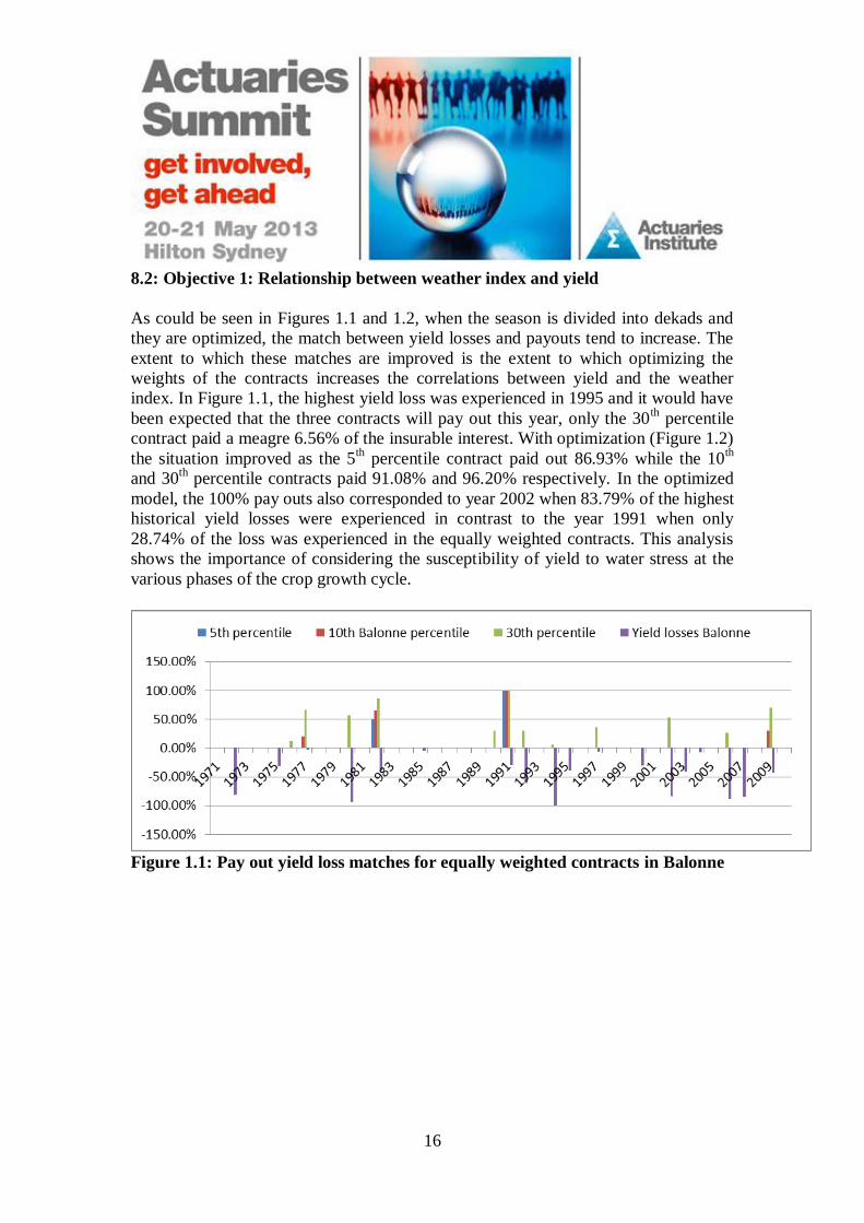
As could be seen in Figures 1.1 and 1.2, when the season is divided into dekads and

they are optimized, the match between yield losses and payouts tend to increase. The

extent to which these matches are improved is the extent to which optimizing the

weights of the contracts increases the correlations between yield and the weather

index. In Figure 1.1, the highest yield loss was experienced in 1995 and it would have

been expected that the three contracts will pay out this year, only the 30th percentile

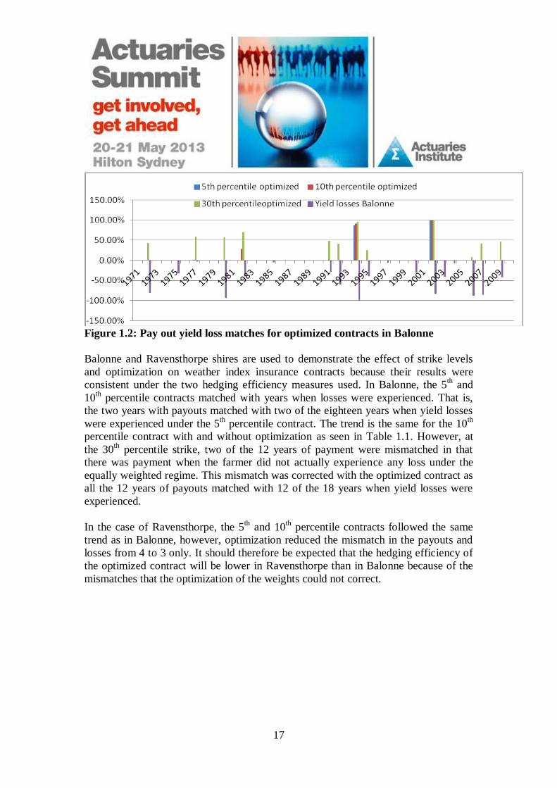
contract paid a meagre 6.56% of the insurable interest. With optimization (Figure 1.2)

the situation improved as the 5th percentile contract paid out 86.93% while the 10

th

and 30th

percentile contracts paid 91.08% and 96.20% respectively. In the optimized

model, the 100% pay outs also corresponded to year 2002 when 83.79% of the highest

historical yield losses were experienced in contrast to the year 1991 when only

28.74% of the loss was experienced in the equally weighted contracts. This analysis

shows the importance of considering the susceptibility of yield to water stress at the

various phases of the crop growth cycle.

Figure 1.1: Pay out yield loss matches for equally weighted contracts in Balonne

17

Figure 1.2: Pay out yield loss matches for optimized contracts in Balonne

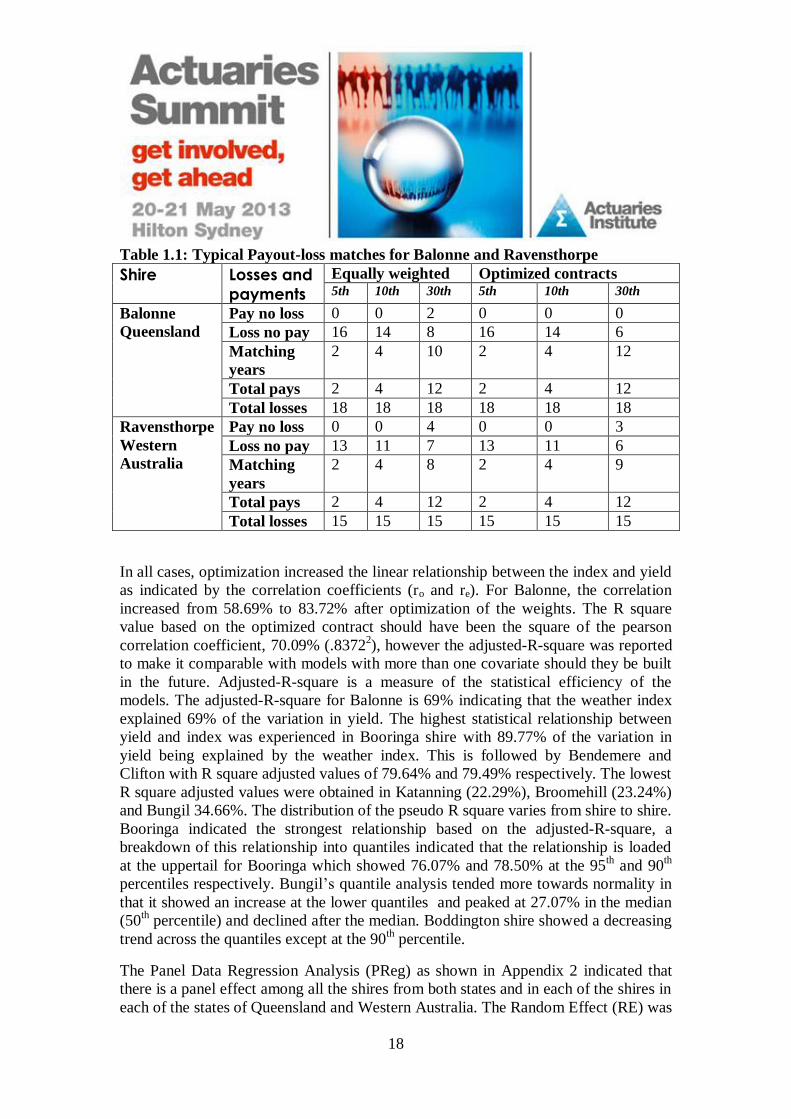
Balonne and Ravensthorpe shires are used to demonstrate the effect of strike levels

and optimization on weather index insurance contracts because their results were

consistent under the two hedging efficiency measures used. In Balonne, the 5th and

10th percentile contracts matched with years when losses were experienced. That is,

the two years with payouts matched with two of the eighteen years when yield losses

were experienced under the 5th percentile contract. The trend is the same for the 10

th

percentile contract with and without optimization as seen in Table 1.1. However, at

the 30th percentile strike, two of the 12 years of payment were mismatched in that

there was payment when the farmer did not actually experience any loss under the

equally weighted regime. This mismatch was corrected with the optimized contract as

all the 12 years of payouts matched with 12 of the 18 years when yield losses were

experienced.

In the case of Ravensthorpe, the 5th and 10

th percentile contracts followed the same

trend as in Balonne, however, optimization reduced the mismatch in the payouts and

losses from 4 to 3 only. It should therefore be expected that the hedging efficiency of

the optimized contract will be lower in Ravensthorpe than in Balonne because of the

mismatches that the optimization of the weights could not correct.

18

Table 1.1: Typical Payout-loss matches for Balonne and Ravensthorpe

Shire Losses and

payments

Equally weighted Optimized contracts 5th 10th 30th 5th 10th 30th

Balonne

Queensland

Pay no loss 0 0 2 0 0 0

Loss no pay 16 14 8 16 14 6

Matching

years

2 4 10 2 4 12

Total pays 2 4 12 2 4 12

Total losses 18 18 18 18 18 18

Ravensthorpe

Western

Australia

Pay no loss 0 0 4 0 0 3

Loss no pay 13 11 7 13 11 6

Matching

years

2 4 8 2 4 9

Total pays 2 4 12 2 4 12

Total losses 15 15 15 15 15 15

In all cases, optimization increased the linear relationship between the index and yield

as indicated by the correlation coefficients (ro and re). For Balonne, the correlation

increased from 58.69% to 83.72% after optimization of the weights. The R square

value based on the optimized contract should have been the square of the pearson

correlation coefficient, 70.09% (.83722), however the adjusted-R-square was reported

to make it comparable with models with more than one covariate should they be built

in the future. Adjusted-R-square is a measure of the statistical efficiency of the

models. The adjusted-R-square for Balonne is 69% indicating that the weather index

explained 69% of the variation in yield. The highest statistical relationship between

yield and index was experienced in Booringa shire with 89.77% of the variation in

yield being explained by the weather index. This is followed by Bendemere and

Clifton with R square adjusted values of 79.64% and 79.49% respectively. The lowest

R square adjusted values were obtained in Katanning (22.29%), Broomehill (23.24%)

and Bungil 34.66%. The distribution of the pseudo R square varies from shire to shire.

Booringa indicated the strongest relationship based on the adjusted-R-square, a

breakdown of this relationship into quantiles indicated that the relationship is loaded

at the uppertail for Booringa which showed 76.07% and 78.50% at the 95th

and 90th

percentiles respectively. Bungil’s quantile analysis tended more towards normality in

that it showed an increase at the lower quantiles and peaked at 27.07% in the median

(50th percentile) and declined after the median. Boddington shire showed a decreasing

trend across the quantiles except at the 90th percentile.

The Panel Data Regression Analysis (PReg) as shown in Appendix 2 indicated that

there is a panel effect among all the shires from both states and in each of the shires in

each of the states of Queensland and Western Australia. The Random Effect (RE) was

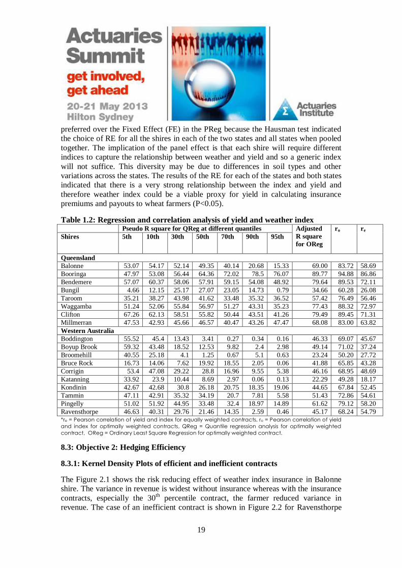
19

preferred over the Fixed Effect (FE) in the PReg because the Hausman test indicated

the choice of RE for all the shires in each of the two states and all states when pooled

together. The implication of the panel effect is that each shire will require different

indices to capture the relationship between weather and yield and so a generic index

will not suffice. This diversity may be due to differences in soil types and other

variations across the states. The results of the RE for each of the states and both states

indicated that there is a very strong relationship between the index and yield and

therefore weather index could be a viable proxy for yield in calculating insurance

premiums and payouts to wheat farmers (P<0.05).

Table 1.2: Regression and correlation analysis of yield and weather index Pseudo R square for QReg at different quantiles Adjusted

R square

for OReg

ro re

Shires 5th 10th 30th 50th 70th 90th 95th

Queensland

Balonne 53.07 54.17 52.14 49.35 40.14 20.68 15.33 69.00 83.72 58.69

Booringa 47.97 53.08 56.44 64.36 72.02 78.5 76.07 89.77 94.88 86.86

Bendemere 57.07 60.37 58.06 57.91 59.15 54.08 48.92 79.64 89.53 72.11

Bungil 4.66 12.15 25.17 27.07 23.05 14.73 0.79 34.66 60.28 26.08

Taroom 35.21 38.27 43.98 41.62 33.48 35.32 36.52 57.42 76.49 56.46

Waggamba 51.24 52.06 55.84 56.97 51.27 43.31 35.23 77.43 88.32 72.97

Clifton 67.26 62.13 58.51 55.82 50.44 43.51 41.26 79.49 89.45 71.31

Millmerran 47.53 42.93 45.66 46.57 40.47 43.26 47.47 68.08 83.00 63.82

Western Australia

Boddington 55.52 45.4 13.43 3.41 0.27 0.34 0.16 46.33 69.07 45.67

Boyup Brook 59.32 43.48 18.52 12.53 9.82 2.4 2.98 49.14 71.02 37.24

Broomehill 40.55 25.18 4.1 1.25 0.67 5.1 0.63 23.24 50.20 27.72

Bruce Rock 16.73 14.06 7.62 19.92 18.55 2.05 0.06 41.88 65.85 43.28

Corrigin 53.4 47.08 29.22 28.8 16.96 9.55 5.38 46.16 68.95 48.69

Katanning 33.92 23.9 10.44 8.69 2.97 0.06 0.13 22.29 49.28 18.17

Kondinin 42.67 42.68 30.8 26.18 20.75 18.35 19.06 44.65 67.84 52.45

Tammin 47.11 42.91 35.32 34.19 20.7 7.81 5.58 51.43 72.86 54.61

Pingelly 51.02 51.92 44.95 33.48 32.4 18.97 14.89 61.62 79.12 58.20

Ravensthorpe 46.63 40.31 29.76 21.46 14.35 2.59 0.46 45.17 68.24 54.79 *re = Pearson correlation of yield and index for equally weighted contracts, ro = Pearson correlation of yield

and index for optimally weighted contracts, QReg = Quantile regression analysis for optimally weighted

contract, OReg = Ordinary Least Square Regression for optimally weighted contract.

8.3: Objective 2: Hedging Efficiency

8.3.1: Kernel Density Plots of efficient and inefficient contracts

The Figure 2.1 shows the risk reducing effect of weather index insurance in Balonne

shire. The variance in revenue is widest without insurance whereas with the insurance

contracts, especially the 30th

percentile contract, the farmer reduced variance in

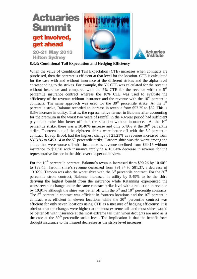
revenue. The case of an inefficient contract is shown in Figure 2.2 for Ravensthorpe

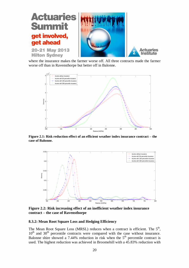
20

where the insurance makes the farmer worse off. All three contracts made the farmer

worse off than in Ravensthorpe but better off in Balonne.

-200 -100 0 100 200 300 400 5000

1

2

3

4

5

6x 10

-3

Revenue (AUD/ha)

Density

Income without insurance

Income with 5th percentile insurance

Income with 10th percentile insurance

Income with 30th percentile insurance

Figure 2.1: Risk reduction effect of an efficient weather index insurance contract – the

case of Balonne.

300 350 400 450 500 550 600 650 700 750 8000

0.005

0.01

0.015

0.02

0.025

Revenue (AUD/ha)

Density

Income without insurance

Income with 5th percentile insurance

Income with 10th percentile insurance

Income with 30th percentile insurance

Figure 2.2: Risk increasing effect of an inefficient weather index insurance

contract – the case of Ravensthorpe

8.3.2: Mean Root Square Loss and Hedging Efficiency

The Mean Root Square Loss (MRSL) reduces when a contract is efficient. The 5th,

10th and 30

th percentile contracts were compared with the case without insurance.

Balonne shire showed a 7.44% reduction in risk when the 5th

percentile contract is

used. The highest reduction was achieved in Broomehill with a 45.83% reduction with

21

the 5th percentile insurance contract. Pingelly shire’s risk increased by 75.08% to be

the worst with the 5th

percentile contract. Only twelve of the 18 shires showed

evidence of risk reductions when MRSL is used as a measure of hedging efficiency at

the 5th percentile. For the 10

th percentile contracts, Broomehill as in the 5

th percentile

contract, has the highest risk reduction with the contract. The risk in Broomehill

reduced by 49.05%. Pingelly shire also has the highest increment in risk under the

10th percentile contract as in the 5

th percentile with an increase of 92.95%. For the 30

th

percentile contract, Pingelly remains the shire with the highest increment in risk of

253.42% but Boyup Brook reduced the semi-variance by 55.33% to be the shire with

the highest risk reduction at the 30th percentile. Twelve of the shires showed risk

reduction with the 5th and 30

th percentile insurance contracts while risks were reduced

for thirteen shires using the 10th percentile contracts.

Table 2.1: Mean Root Square Loss Analyses

Shires by

states

Without

contract

Strikes in percentiles

5th 10th 30th With

contract

($)

Chang

es (%)

With

contract

($)

Changes

(%)

With

contract($)

Changes (%)

QLD

Balonne 68.80 63.68 -7.44 63.46 -7.76 47.94 -30.32

Booringa 57.22 57.63 0.72 59.59 4.14 56 -2.13

Bendemere 69.61 65.69 -5.63 64.84 -6.85 58.21 -16.38

Bungil 76.76 74.39 -3.09 74.09 -3.48 78.8 2.66

Taroom 76.16 78.43 2.98 80.61 5.84 71.86 -5.65

Waggamba 66.39 62.84 -5.35 63.47 -4.40 55.25 -16.78

Clifton 61.78 56.59 -8.40 55.83 -9.63 48.96 -20.75

Millmerran 49.48 49.44 -0.08 48.61 -1.76 47.09 -4.83

WA

Boddington 42.97 32.53 -24.30 25.56 -40.52 29.43 -31.51

Boyup Brook

78.68 45.52 -42.15 43.27 -45.01 35.15 -55.33

Broomehill 65.5 35.48 -45.83 33.37 -49.05 53.95 -17.63

Bruce

Rock

40.37 33.86 -16.13 30.92 -23.41 33.54 -16.92

Corrigin 42.83 39.77 -7.14 40.06 -6.47 45.65 6.58

Katanning 51.34 32.18 -37.32 35.62 -30.62 64.11 24.87

Kondinin 27.8 30.53 9.82 30.15 8.45 32.43 16.65

Tammin 33.72 35.8 6.17 32.2 -4.51 33.09 -1.87

Pingelly 9.79 17.14 75.08 18.89 92.95 34.6 253.42

Ravensthor

pe

17.76 19.21 8.16 24.4 37.39 46.16 159.91

22

8.3.3: Conditional Tail Expectation and Hedging Efficiency

When the value of Conditional Tail Expectation (CTE) increases when contracts are

purchased, then the contract is efficient at that level for the location. CTE is calculated

for the case with and without insurance at the different strikes and the alpha level

corresponding to the strikes. For example, the 5% CTE was calculated for the revenue

without insurance and compared with the 5% CTE for the revenue with the 5th

percentile insurance contract whereas the 10% CTE was used to evaluate the

efficiency of the revenue without insurance and the revenue with the 10th percentile

contracts. The same approach was used for the 30th percentile strike. At the 5

th

percentile strike, Balonne recorded an increase in revenue from $57.25 to $62. This is

8.3% increase in utility. That is, the representative farmer in Balonne after accounting

for the premium in the worst two years of rainfall in the 40-year period had sufficient

payout to make him better off than the situation without insurance. At the 10th

percentile strike, there was a 10.40% increase and only 5.49% at the 30th percentile

strike. Fourteen out of the eighteen shires were better off with the 5th

percentile

contract. Boyup Brook had the highest change of 21.21% as revenue increased from

$373.86 to $453.14 at the 5th percentile strike. Taroom shire was the worst among the

shires that were worse off with insurance as revenue declined from $60.15 without

insurance to $50.50 with insurance implying a 16.04% decrease in revenue for the

representative farmer in the shire over the period in view.

For the 10th percentile contract, Balonne’s revenue increased from $90.26 by 10.40%

to $99.65. Taroom shire’s revenue decreased from $91.34 to $81.37, a decrease of

10.92%. Taroom was also the worst shire with the 5th percentile contract. For the 30

th

percentile strike contract, Balonne increased in utility by 5.49% to be the shire

deriving the highest benefit from the insurance while Katanning experienced the

worst revenue change under the same contract strike level with a reduction in revenue

by 10.91% although the shire was better off with the 5th

and 10th

percentile contracts.

The 5th

percentile contract was efficient in fourteen locations and the 10th

percentile

contract was efficient in eleven locations while the 30th

percentile contract was

efficient for only seven locations using CTE as a measure of hedging efficiency. It is

obvious that the changes were highest at the most extreme tails and most shires would

be better off with insurance at the most extreme tail than when droughts are mild as is

the case at the 30th

percentile strike level. The implication is that the benefit from

drought insurance to the insured decreases as the strike level increases.

23

Table 2.2: Conditional Tail Expectations Analysis of Queensland and Western

Australian shires. 5% strike 10% strike 30% strike

Shires

Without

contract

($)

With

contract

($)

Change

(%)

Without

contract

($)

With

contract

($)

Change

(%)

Without

contract

($)

With

contract

($)

Change

(%)

QLD

Balonne 57.25 62 8.30 90.26 99.65 10.40 183.47 193.54 5.49

Booringa 118.83 121.79 2.49 136.65 134.35 -1.68 186.07 187.48 0.76

Bendemere 129.48 145.06 12.03 165.97 179.15 7.94 247.33 256.68 3.78

Bungil 145.17 151.79 4.56 170.06 172.45 1.41 252.22 260.41 3.25

Taroom 60.15 50.5 -16.04 91.34 81.37 -10.92 193 194.11 0.58

Waggamba 114.05 120.52 5.67 141.07 145.43 3.09 220.43 230.39 4.52

Clifton 342.88 350.63 2.26 376.54 385.95 2.50 459.14 452.44 -1.46

Millmerran 300.89 279.19 -7.21 325.45 322.85 -0.80 385.44 380.94 -1.17

WA

Boddington 390.91 415.88 6.39 438.58 459.53 4.78 488.62 465.15 -4.80

Boyup Brook 373.86 453.14 21.21 456.75 497.07 8.83 537.23 537.56 0.06

Broomehill 364.3 432.68 18.77 431.78 461.61 6.91 501.46 464.7 -7.33

Bruce Rock 257.9 280.1 8.61 293.83 306.74 4.39 345.72 333.73 -3.47

Corrigin 274.25 291.02 6.11 309.12 314.22 1.65 362.55 343.67 -5.21

Katanning 388.88 427.52 9.94 433.16 440.06 1.59 490.32 436.84 -10.91

Kondinin 318.56 319.11 0.17 334.23 330.37 -1.15 368.07 357.24 -2.94

Tammin 382.56 383.29 0.19 411.15 410.93 -0.05 452.88 436.18 -3.69

Pingelly 428.35 418.06 -2.40 433.53 417.43 -3.71 447.39 408.7 -8.65

Ravensthorpe 370.11 368.12 -0.54 382.6 376.76 -1.53 406.96 367.92 -9.59

8.4: Objective 3: Diversification

8.4.1: The effect of temporal risk pooling on a portfolio of weather index insurance contracts

For the 5

th percentile contract in Table 3.1, the probability of a high profit was highest

for a single year and two year pooling but this is also associated with high probability

of loss. The lowest probability of loss ratio being less than 0.5 occurs when risk is

pooled over ten years (19%). This decline from 73% for a single year pooling to only

19% for a ten-year pool is the cost of having no loss ratio greater than 3 for the ten

year risk pooling. This trend persisted across the other strike levels. In addition, an

increase in strike levels further tempered the risk in that the probability of extreme

values decreases as movements are made to higher strike levels across the various

years of pooling. This climaxed in zero probabilities for loss ratios less than 0.5 and

greater than 3 for the 30th

percentile strikes for ten years of risk pooling. Hence, one

could conclude that temporal risk pooling, particularly at higher strike levels reduces

systemic risk to the insurer. This analysis confirms the intuition that drought risks are

most systemic at the tail in that extreme drought will affect several locations

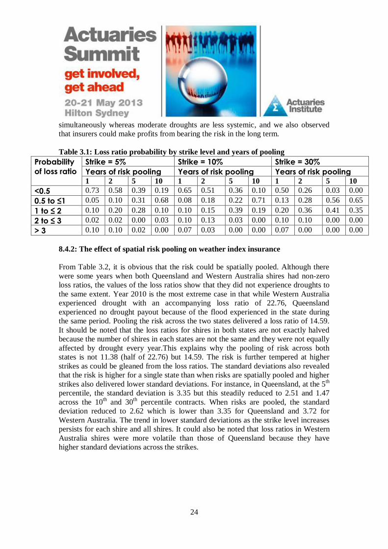
24

simultaneously whereas moderate droughts are less systemic, and we also observed

that insurers could make profits from bearing the risk in the long term.

Table 3.1: Loss ratio probability by strike level and years of pooling

Probability

of loss ratio

Strike = 5% Strike = 10% Strike = 30%

Years of risk pooling Years of risk pooling Years of risk pooling 1 2 5 10 1 2 5 10 1 2 5 10

<0.5 0.73 0.58 0.39 0.19 0.65 0.51 0.36 0.10 0.50 0.26 0.03 0.00

0.5 to ≤1 0.05 0.10 0.31 0.68 0.08 0.18 0.22 0.71 0.13 0.28 0.56 0.65

1 to ≤ 2 0.10 0.20 0.28 0.10 0.10 0.15 0.39 0.19 0.20 0.36 0.41 0.35

2 to ≤ 3 0.02 0.02 0.00 0.03 0.10 0.13 0.03 0.00 0.10 0.10 0.00 0.00

> 3 0.10 0.10 0.02 0.00 0.07 0.03 0.00 0.00 0.07 0.00 0.00 0.00

8.4.2: The effect of spatial risk pooling on weather index insurance

From Table 3.2, it is obvious that the risk could be spatially pooled. Although there

were some years when both Queensland and Western Australia shires had non-zero

loss ratios, the values of the loss ratios show that they did not experience droughts to

the same extent. Year 2010 is the most extreme case in that while Western Australia

experienced drought with an accompanying loss ratio of 22.76, Queensland

experienced no drought payout because of the flood experienced in the state during

the same period. Pooling the risk across the two states delivered a loss ratio of 14.59.

It should be noted that the loss ratios for shires in both states are not exactly halved

because the number of shires in each states are not the same and they were not equally

affected by drought every year.This explains why the pooling of risk across both

states is not 11.38 (half of 22.76) but 14.59. The risk is further tempered at higher

strikes as could be gleaned from the loss ratios. The standard deviations also revealed

that the risk is higher for a single state than when risks are spatially pooled and higher

strikes also delivered lower standard deviations. For instance, in Queensland, at the 5th

percentile, the standard deviation is 3.35 but this steadily reduced to 2.51 and 1.47

across the 10th and 30

th percentile contracts. When risks are pooled, the standard

deviation reduced to 2.62 which is lower than 3.35 for Queensland and 3.72 for

Western Australia. The trend in lower standard deviations as the strike level increases

persists for each shire and all shires. It could also be noted that loss ratios in Western

Australia shires were more volatile than those of Queensland because they have

higher standard deviations across the strikes.

25

Table 3.2: Estimated Annual Loss Ratios at different strike levels

Year Strike = 5% Strike = 10% Strike = 30% QLD WA All QLD WA All QLD WA All

1971 0.00 0.00 0.00 0.00 0.00 0.00 0.00 0.16 0.09

1972 1.21 0.00 0.43 1.11 0.80 0.92 2.48 1.92 2.15

1973 0.00 0.00 0.00 0.00 0.00 0.00 0.00 0.00 0.00

1974 0.00 0.00 0.00 1.38 0.00 0.55 0.64 0.00 0.26

1975 0.00 0.00 0.00 0.00 0.00 0.00 0.56 0.00 0.23

1976 0.00 0.00 0.00 0.00 0.00 0.00 0.00 0.24 0.14

1977 8.58 0.00 3.08 7.33 0.03 2.94 5.18 0.57 2.44

1978 0.00 0.00 0.00 0.00 0.00 0.00 0.00 0.33 0.20

1979 0.00 0.00 0.00 0.55 0.00 0.22 0.53 0.83 0.71

1980 0.00 6.13 3.93 0.21 5.75 3.54 2.50 3.66 3.19

1981 0.00 0.19 0.12 0.00 0.79 0.48 0.00 1.21 0.72

1982 3.44 1.07 1.92 4.97 0.84 2.49 2.80 1.19 1.85

1983 0.00 0.00 0.00 0.00 0.00 0.00 0.00 0.41 0.24

1984 0.00 0.00 0.00 0.00 0.00 0.00 0.00 0.03 0.02

1985 0.00 0.00 0.00 0.00 0.14 0.08 0.00 1.84 1.09

1986 0.00 0.00 0.00 0.00 0.00 0.00 0.30 0.20 0.24

1987 0.00 3.08 1.98 0.00 2.40 1.44 0.07 2.02 1.23

1988 0.00 0.00 0.00 0.00 0.00 0.00 0.00 0.25 0.15

1989 0.00 0.00 0.00 0.00 0.00 0.00 0.39 0.35 0.36

1990 0.00 0.00 0.00 0.00 0.19 0.11 0.41 0.99 0.75

1991 0.09 0.00 0.03 3.99 0.00 1.59 3.65 0.07 1.52

1992 0.00 0.00 0.00 0.25 0.00 0.10 2.24 0.00 0.91

1993 0.00 0.00 0.00 0.04 0.00 0.02 0.86 0.00 0.35

1994 19.30 0.42 7.20 12.98 1.21 5.91 5.82 2.58 3.89

1995 0.00 0.00 0.00 0.00 0.00 0.00 0.78 0.00 0.31

1996 0.00 0.00 0.00 0.00 0.00 0.00 0.00 0.36 0.21

1997 0.00 0.00 0.00 0.00 0.00 0.00 0.00 0.82 0.49

1998 0.00 0.00 0.00 0.00 0.00 0.00 0.00 0.15 0.09

1999 0.00 0.00 0.00 0.00 0.00 0.00 0.07 0.00 0.03

2000 0.00 1.70 1.09 0.00 2.80 1.68 0.91 3.66 2.54

2001 0.00 2.96 1.90 0.00 4.59 2.76 0.00 2.55 1.52

2002 2.37 0.00 0.85 3.63 1.19 2.17 2.67 1.75 2.12

2003 0.00 0.00 0.00 0.00 0.00 0.00 0.42 0.00 0.17

2004 1.67 0.00 0.60 1.50 0.00 0.60 1.09 0.95 1.01

2005 0.00 0.00 0.00 0.00 0.00 0.00 0.00 0.01 0.01

2006 3.35 1.68 2.28 2.06 1.37 1.65 1.69 1.95 1.85

2007 0.00 0.00 0.00 0.00 0.03 0.02 0.88 0.50 0.66

2008 0.00 0.00 0.00 0.00 0.07 0.04 0.00 0.60 0.36

2009 0.00 0.00 0.00 0.00 0.00 0.00 3.04 0.15 1.33

2010 0.00 22.76 14.59 0.00 17.80 10.70 0.00 7.69 4.57

Mean 1.00 1.00 1.00 1.00 1.00 1.00 1.00 1.00 1.00

SD 3.35 3.72 2.62 2.51 3.00 2.03 1.47 1.48

1.12

26

9. Discussion

Capturing the relative exposure of crops to risk at their different phenological stages

is necessary to improve the relationship between yield and weather index as earlier

noted in the work of Stoppa and Hess (2003). This could be achieved through

optimization and expert weighting. We have used only the optimized model in this

study. It was thought that hedging efficiency should result from the alteration of the

distribution of the statistical efficiency across the quantiles on the yield–index

relationship continuum as shown in the ordinary least square regression and quantile

regression analyses. However, Vedenov and Barnett (2004) have shown that a strong

statistical relationship between yield and index does not guarantee efficiency as we

have also noted in this study. One could have insinuated that when the relationship is

stronger at the lower tail there will be higher efficiency. This is true as in the cases of

Balonne and Bendemere with higher relationships at the 5th, 10

th and 30

th percentiles

than their corresponding upper tail quantiles but the cases of Pingelly and

Ravensthorpe contradicted this possible conclusion. More complex multi-trigger

indices may have to be designed to capture the relationship required for significant

improvements in hedging efficiency. The other variables may include soil moisture

and temperature.

Furthermore, the pricing of weather index insurance contract does not capture the

relative efficiency of the contracts. The most expensive contracts are not necessarily

the most efficient and the cheapest contracts are not necessarily the least efficient. It

seems that the actuarial burns analysis does not capture the relative efficiency of the

contracts. This finding alludes to previous conclusions that data availability and

methodological issues are among the bottlenecks hindering the proliferation of

weather index insurance (Vedenov & Barnett 2004; Jewson & Brix 2005).

In addition, our panel data analysis for each of the two states and the two states,

combined, indicated that there was a panel effect. The implication is that weather

indices would have to be designed to capture geographical diversity in order to

capture differences like soil types. This study concurs with the recommendation by

scholars like Vedenov and Barnett (2004) on the localization of weather index

contracts. Unfortunately, the localization of the contract will erode the cost savings

anticipated from the use of weather index insurance. This is because the insurer will

not be able to take advantage of economy of scale in the design of the product.

Another major finding of our study is that drought risk to the insurer is inversely

proportional to strike levels, years of pooling and spatial pooling. These findings are

in congruence with those of Chantarat (2009). Bardsley, Abey and Davenport (1984)

implied that risk pooling could make weather index insurance more viable in

Australia as we have equally noted. We further observed that the reduction in risk to

the insurer’s portfolio arising from increase in contract strike comes at the cost of

27

reduced benefits to the insured. The analyses obviously captured the year 2010 flood

and drought in Queensland and Western Australia respectively in that there was a

very heavy payout in Western Australia but none in Queensland (Agnew 2011; Hicks

2011).

Hedging efficiency depends on the risk measures used particularly at the higher

strikes. Although, the MRSL (Mean Root Square Loss) reduced the semi-variance in

revenue, it does not always lead to higher revenues in years when droughts are

experienced. However, the risk measures are more congruent at the extreme tail. For

instance, MRSL indicated efficiency for 12 shires, only one of them contradicted the

results from the CTE (Conditional Tail Expectation) at the 5th percentile strike. At the

10th percentile strike, there were 13 shires benefiting from the contract based on

MRSL but the CTE missed two of them. In the case of the 12 shires MRSL flagged as

deriving value from the 30th

percentile contracts, 6 of them were not captured by

CTE. The incongruence in the efficiency measures increased with the strike levels.

Generally, it seems that the MRSL does not respond to strike leves like the CTE. The

number of locations flagging efficiency reduced with the strke level under the CTE

efficiency test whereas there seems to be a relative consistency of hedging efficiency

across locations with the MRSL. The findings of Vedenov and Barnett (2004) are

similar to ours in that they used three efficiency measures and the efficiency results

were found to be closely related but not perfectly the same.

Our study therefore suggests that insurers will be more comfortable bearing modest

risk over the long term than the most extreme risks over the short term. To bear the

extreme tail risk like the 5th

percentile contracts, reinsurance cost may have to be

factored into the pricing of the contract making it more expensive for farmers. It is

however reasonable to expect that the Australian community may still be better off

insuring the risk of drought than following the current pattern of risk management as

noted in Quiggin and Chambers (2004) . It is also expected that experience, over time,

will prove the worth of the insurance as insured farmers weather the storms of

droughts unlike their uninsured counterparts. The effect of the insurance could also be

tempered as farmers pass on part of the cost to consumers. This implies that the

society at large bears the cost of the insurance and therefore the problem of equity or

politicization of drought response would not arise. This arrangement should be more

equitable in that the proportion of the insurance an individual pays indirectly by

buying the product is the extent to which the individual has consumed the product

whereas, spending public tax payers fund to bail out farmers translates into an

assumption that everyone consumes the product to an equal extent. The equity debate

and politicization of drought response remain major considerations in the current

Australian Drought Policy (Kimura & Anton 2011).

28

10. Conclusions and recommendations

The pricing of weather index insurance contracts would have to be localized thereby

reducing the cost reduction benefits anticipated from its usage. Also, the use of

actuarial burns analysis for the pricing appears to be pareto-inefficient in that it does

not reflect the relative exposure of the locations to risk and hedging efficiency. We

also noted that statistical efficiency does not proportionately translate into hedging

efficiency. The insurer could temper the risk of a portfolio of weather index insurance

contract by spatially and temporally pooling the risks. Higher strike contracts are

more diversifiable than the lower strike contracts that correspond to the very extreme

tail events and could require reinsurance. The insurer interested in weather index

insurance could only look forward to profit in the long run.

We recommend that researchers and practitioners investigate further into the

methodological frameworks appropriate for the pricing of weather index insurance

contracts and measurement of its efficiency. In addition, appropriate legal frameworks

are required to enhance appropriate use of the products.

29

References

ABS 2012, Australian Bureau of Statistics, <http://www.abs.gov.au/>

Acerbi, C & Tasche, D 2001, 'Expected Shortfall: a natural coherent alternative to

Value at Risk'.

Adeyinka, A & Kaino, L 2012, 'Quantile Analysis of the Mathematics

Achievement - Attitude Relationship by Gender ', European Journal of Social

Sciences, vol. 34, no. 3, pp. 452-60

Agnew, PFA 2011, Flood horror and tragedy, Agnew P & F Association Inc,

Brisbane.

Ahsan, SM, Ali, AAG & Kurian, NJ 1982, 'Toward a theory of agricultural

insurance', American Journal of Agricultural Economics, vol. 64, no. 3, pp. 510-

29.

Bardsley, P 1986, 'A note on the viability of rainfall insurance—reply', Australian

Journal of Agricultural and Resource Economics, vol. 30, no. 1, pp. 70-5.

Bardsley, P, Abey, A & Davenport, SV 1984, 'The economics of insuring crops

against drought', Australian Journal of Agricultural and Resource Economics, vol.

28, no. 1, pp. 1-14.

Bernstein, P 1996, Against the Gods: The Remarkable Story of Risk, John Wiley

and Sons.

Binswanger-Mkhize, HP 2012, 'Is there too much hype about index-based

agricultural insurance?', Journal of Development Studies, vol. 48, no. 2, p. 14.

Bodie, Z & Merton, RC 1998, Finance, Prentice Hall, Upper Saddle River NJ.

Bokusheva, R 2011, 'Measuring dependence in joint distributions of yield and

weather variables', Agricultural Finance Review, vol. 71, no. 1, pp. 120-41.

BoM, 2012, Rainfall deficiencies Retrieved 22nd December 2012, from <http://www.bom.gov.au/climate/drought/#tabs=4>

Botterill, LC & Wilhite, DA 2005, From disaster response to risk management:

Australia's National Drought Policy, vol. 22, Springer.

30

Chantarat, S 2009, 'Pro-poor risk management: essays on the economics of index-

based risk transfer products', Cornell University Faculty of the Graduate School.

Chantarat, S, Barrett, CB, Mude, AG & Turvey, CG 2007, 'Using weather index

insurance to improve drought response for famine prevention', American Journal

of Agricultural Economics, vol. 89, no. 5, pp. 1262-8.

Chantarat, S, Mude, AG, Barrett, CB & Carter, MR 2012, 'Designing Index-Based

Livestock Insurance for Managing Asset Risk in Northern Kenya', Journal of Risk

and Insurance, vol. Early view before inclusion in an issue.

Clifton, 2012 <http://en.wikipedia.org/wiki/Clifton,Queensland>

Cuevas, SC 2011, 'Climate change, vulnerability, and risk linkages', International

Journal of Climate Change Strategies and Management, vol. 3, no. 1, pp. 29-60.

Dai, A, Trenberth, KE & Qian, T 2004, 'A global dataset of palmer drought

severity index for 1870-2002: relationship with soil moisture and effects of

surface warming', American Meteorological Society, p. 13.

Ghiulnara, A & Viegas, C 2010, 'Introduction of weather-derivative concepts:

perspectives for Portugal', Journal of Risk Finance, The, vol. 11, no. 1, pp. 9-19.

Gumbel, EJ 1958, Statistics of extremes, Columbia University Press, New York.

Gurenko, EN 2006, Climate change and insurance: Disaster risk financing in

developing countries, vol. 6, Earthscan/James & James.

Harwood, JL, Heifner, R, Coble, K, Perry, J & Somwaru, A 1999, Managing risk

in farming: concepts, research, and analysis, US Department of Agriculture,

Economic Research Service.

Hayman, P & Cox, P 2005, 'Drought risk as a negotiated construct', in LC

Botterill & DA Wilhite (eds), From disaster response to risk management :

Australia's National Drought Policy, Springer Netherlands, vol. 22.

Hicks, P 2011, Budget 2010–11: Rural affairs, Parliament of Australia, viewed

10th May,

<http://www.aph.gov.au/About_Parliament/Parliamentary_Departments/Parliame

ntary_Library/pubs/rp/BudgetReview201011/DroughtMeasures>.

Hoeppe, P & Gurenko, EN 2006, 'Scientific and economic rationales for

innovative climate insurance solutions', Climate Policy, vol. 6, no. 6, pp. 607-20.

31

Jewson, S & Brix, A 2005, Weather derivative valuation: the meteorological,

statistical, financial and mathematical foundations, Cambridge University Press.

Just, RE, Calvin, L & Quiggin, J 1999, 'Adverse selection in crop insurance:

Actuarial and asymmetric information incentives', American Journal of

Agricultural Economics, vol. 81, no. 4, pp. 834-49.

Kapphan, I 2012, Weather risk management in the light of climate change using

financial derivatives, a PhD dissertation submitted to Eidgenössische Technische

Hochschule (ETH) , Zurich.

Kapphan, I, Calanca, P & Holzkaemper, A 2011, Climate Change, Weather

Insurance Design and Hedging Effectiveness, Working Paper 17, Institute for

Environmental Decisions (IED), Zurich, volume 37 document 2.

Kapphan, I, Calanca, P & Holzkaemper, A 2012, 'Climate Change, Weather

Insurance Design and Hedging Effectiveness', The Geneva Papers on Risk and

Insurance-Issues and Practice, vol. 37, no. April, p. 286.

Keenan, T & Cleugh, H 2011, Climate science update: a report to the 2011

Garnaut Review, Centre for Australian Weather and Climate Research.

Kelly, DSL & Ball, ML 1991, Principles of Insurance Law in Australia and New

Zealand, Butterworths.

Kimball-Stanley, A 2008, 'Insurance and Credit Default Swaps: Should Like

Things Be Treated Alike', Conn. Ins. LJ, vol. 15, p. 241.

Kimura, S & Antón, J 2011, Risk management in agriculture in Australia, OECD

Publishing.

Koenker, R 2005, Quantile Regresssion, Wiley Online Library.

Kokic, P, Nelson, R, Meinke, H, Potgieter, A & Carter, J 2007, 'From rainfall to

farm incomes—transforming advice for Australian drought policy. I.

Development and testing of a bioeconomic modelling system', Crop and Pasture

Science, vol. 58, no. 10, pp. 993-1003.

Lindesay, JA 2005, ' Climate and Drought in the Subtropics - The Australian

Example', in LC Botterill & DA Wilhite (eds), From Disaster Response to Risk

Management : Australia's National Drought Policy, Springer, Netherlands, vol.

22.

32

Meuwissen, MPM, Van Asseldonk, MAPM & Huirne, RBM 2008, Income

Stabilisation in European Agriculture: Design and Economic Impact of Risk

Management Tools, Wageningen Academic Pub.

Miranda, MJ & Glauber, JW 1997, 'Systemic risk, reinsurance, and the failure of

crop insurance markets', American Journal of Agricultural Economics, vol. 79, no.

1, pp. 206-15.

Nieto, JD, Fisher, M, Cook, S, Läderach, P & Lundy, M 2012, 'Weather Indices

for Designing Micro-Insurance Products for Small-Holder Farmers in the Tropics',

PloS one, vol. 7, no. 6, June e38281.

Niskanen, WA 1971, Bureaucracy and representative government, Aldine

Atherton, Chicago.

OECD 2011, Risk management in agriculture: What role for government?

Published by Organization for Economic Co-operation and Development retrieved

from; <http://www.oecd.org/tad/agricultural-policies/49003833.pdf>

O’Meagher, B 2005, 'Policy for agricultural drought in Australia: an economic

perspective', in LC Botterill & DA Wilhite (eds), From disaster response to risk

management : Australia's National Drought Policy, Springer, Netherlands, vol.

22.

Parry, ML, Canziani, OF, Palutikof, JP, van der Linden, PJ & Hanson, CE 2007,

IPCC, 2007: climate change 2007: impacts, adaptation and vulnerability.

Contribution of working group II to the fourth assessment report of the

intergovernmental panel on climate change, Cambridge University Press,

Cambridge.

Potgieter, A B, Hammer, GL & Doherty, A 2011, Oz-Wheat: A regional scale

crop yield simulation model for Australian wheat, Queensland Department of

Primary Industries and Fisheries, Brisbane.

Quiggin, J 1994, 'The optimal design of crop insurance', in DL Hueth & WH

Furtan (eds), Economics of agricultural crop insurance: theory and evidence,

Kluwer Academic Publishers, Boston.

Quiggin, J & Chambers, RG 2004, 'Drought policy: a graphical analysis', The

Australian Journal of Agricultural and Resource Economics, vol. 48, no. 2, p. 27.

Quiggin, J, Karagiannis, G & Stanton, J 1994, 'Crop insurance and crop

production: An empirical study of moral hazard and adverse selection', in DL

33

Hueth & H Furman (eds), Economics of agricultural crop insurance: theory and

evidence Springer, vol. 4.

Quiggin, JC 1986, 'A note on the viability of rainfall insurance', Australian

Journal of Agricultural and Resource Economics, vol. 30, no. 1, pp. 63-9.

Raspe, A 2002, 'Legal and regulatory issues', in E Banks (ed.), Weather Risk

Management: Markets, Products, and Applications, Palgrave, New York.

Sharma, AK & Vashishtha, A 2007, 'Weather derivatives: risk-hedging prospects

for agriculture and power sectors in India', Journal of Risk Finance, vol. 8, no. 2,

pp. 112 - 32

Skees, JR & Collier, B 2012, 'The roles of weather insurance and the carbon

market', in D Köhn (ed.), Greening the Financial Sector: How to Mainstream

Environmental Finance in Developing Countries, Springer, Berlin Heidelberg.

Smith, VH & Glauber, JW 2012, 'Agricultural Insurance in Developed Countries:

Where Have We Been and Where Are We Going?', Applied Economic

Perspectives and Policy.

Stoppa, A & Hess, U 2003, 'Design and use of weather derivatives in agricultural

policies: the case of rainfall index insurance in Morocco', in the proceedings of

International Conference on Agricultural policy reform and the WTO: where are

we heading? Capri, Italy, June 23 - 26.

Turvey, C 2001, 'Weather insurance and specific event risks in agriculture',

Review of Agricultural Economics, vol. 23, no. 2, pp. 333- 51.

Vedenov, DV & Barnett, BJ 2004, 'Efficiency of Weather Derivatives as Primary

Crop Insurance Instruments', Journal of Agricultural and Resource Economics,

vol. 29, no. 3, pp. 387-403.

Vortex 2012, Vortex insurance agency,

<http://www.vortexinsuranceagency.com/AboutUs/InsuranceOrDerivative.aspx >.

Wilhite, DA 2005, 'Drought policy and preparedness: the Australian experience in

an international context', in LC Botterill & DA Wilhite (eds), From disaster

response to risk management : Australia's National Drought Policy, Springer,

Netherlands, vol. 22.

34

Wright, BD & Hewitt, JA (eds) 1994, All-risk crop insurance: lessons from theory

and experience, in Economics of Agricultural Crop Insurance, Kluwer Academic

Publishers, Norwell MA.

Yang, CC, Brockett, PL & Wen, MN 2009, ‘Basis risk and hedging efficiency of

weather derivatives’, The Journal of Risk Finance, vol. 10, no. 5, pp. 517-316.

Yang, CC, Li, LS & Wen, MM 2010, 'Weather risk hedging in the European

markets and international investment diversification', The Geneva Risk and

Insurance Review, vol. 36, no. 1, pp. 74-94.

Zeuli, KA & Skees, JR 2005, 'Rainfall insurance: A promising tool for drought

management', Water Resources Development, vol. 21, no. 4, pp. 663-75.

Zweifel, P & Eisen, R 2012, Insurance Economics, Springerverlag Berlin

Heidelberg.

35

Appendices

Appendix 1: Pricing of optimized insurance contracts in percentage

States and

shires

Strike levels in

percentiles

States and

shires

Strike levels in percentiles

5th

5th

10th

30th WA

5th

10th

30th QLD

Balonne 4.67 5.55 15.90 Boddington 2.84 4.32 9.11

Booringa 4.07 5.20 14.71 Boyup Brook 3.19 3.44 6.84

Bendemere 4.45 5.07 15.00 Broomehill 4.83 5.22 14.35

Bungil 3.40 4.56 13.00 Bruce Rock 3.84 5.34 11.23

Taroom 3.79 6.76 17.69 Corrigin 3.84 5.49 15.43

Waggamba 2.71 6.16 16.57 Katanning 3.92 7.45 16.37

Clifton 3.23 6.97 14.63 Kondinin 3.82 5.32 8.98

Millmerran 4.73 5.15 11.11 Tammin 3.16 4.66 9.78

Pingelly 2.51 5.26 11.11

Ravensthorp

e

2.68 4.56 13.18

Appendix 2: The results of the random model for the shires in all and each state.

Locations Y Coefficient Standard

error

Z P>\z\ 95%Confidence

Interval limits

R-Square Wald Chi Prob Chi

Lower Upper

All shires p 2.12 0.07 29.30 0.00 1.98 2.26 0.0000 858.68 0.00

0.0000

0.5446

Constant 1.03-09 0.02 0.00 1.00 -0.05 0.05

QLD

shires

P 2.10 0.08 26.43 0.00 1.94 2.26 0.0000 698.56 0.00

0.0000 constant 1.51-09 0.03 0.00 1.00 -0.06 0.06 0.6872

WA shires p 2.10 0.08 26.43 0.00 1.94 2.26 0.0000 698.56 0.00

0.0000 constant 1.51-09 0.03 0.00 1.00 -0.06 0.06 0.6872