Embed Size (px)
Citation preview

VI. Economics ofBrown Shale Gas Production
VI. Economics ofBrown Shale Gas Production
There are three principal areas of uncertainty inevaluating the commercial potential of naturalgas production from the Devonian shales. Thesebasic uncertainties are:
. economic
● technological, and
● geologic.
The economic uncertainties involve primarilyexpected well head prices and the tax treatmentof income from natural gas production, buteconomic uncertainty also intersects technologi-cal uncertainty. The areas of intersection involvepossible progress in drilling technology and theeffects of stimulation techniques on production.The principal geologic uncertainty involves theBrown shale resource base, i.e., how much of theBrown shale is a high-quality, gas-productiveresource, how much is medium quality, and howmuch is low quality? As natural gas prices in-crease to reflect the value of this resource moreclosely, it is reasonable to expect that relativelylarge amounts of shale gas might becomeeconomically attractive. What is not now ade-quately known, and can only be determined fromactual drilling and production experience over awide geographic area, is the quantity of high-,medium-, and low-quality areas of Brown shale. ’
The approach used here is to deal witheconomic uncertainty by considering a range ofwellhead prices and tax treatments. These rangesof price and tax cases are used to evaluate theafter-tax net-present values (ATNPV—Currentworth of a flow of income after taxes); of gaswells dri l led into the Brown shale in threegeographic localities in the Appalachian Basin.The drilling costs, dry-hole experience, and pro-
I See the section titled [xtent of the Economically Pro-ducible Area for rationale used to estimate the quantity ofcommercially productive Brown shale In the AppalachianBasin,
duction profile information used in the ATNPVcalculations are the actual data for each of thethree Iocalities,2 and each locality is evaluatedseparately. J The three were chosen as examplesof high-, medium-, and lower-quality resourcesfor which adequate data were available on aconsistent basis to support ATNPV calculationsunder alternative assumptions concerning theprice and tax determinants of economic incen-tives. It must be realized that these threelocalities are situated in a small area of the Ap-palachian Basin which is known to be gas pro-ductive. Therefore, the terms high-quality,medium-quality, and low-quality resource arerelative to each other only, and production datafrom these three localities cannot be extrapolateddirectly to the entire 163,000-square-mileextent ofthe Appalachian Basin.
Production data from 490 shale wells in thegas-productive area of the Appalachian Basinwere used to estimate the potential productionfrom other areas of the Appalachian Basin whereshale gas production might be economicallyfeasible. This part of the analysis is the point ofmost crucial interest and the weakest link in theoverall analysis, Until substantially more drillinghas been done over a wide area, the amount ofthe Brown shale resource with economic poten-tial will not be known with any more confidencethan the judgmentally plausible estimates used in
zThe after. tax net-present value (A TNPV) calculations
were made with the aid of a computer ized rout inedeveloped by Drs, Robert Kalter and Wallace Tyner. ThisATNPV calculation routine is described in Wallace E, Tyner
and Robert ]. Kalter, “A Simulation Model for ResourcePolicy Evaluation, ” Cornell Agricultural Economics StaffPaper No. 76-35, November 1976.
3These ind iv Idual local i t ies a r e n o t h o m o g e n e o u s I n
terms of either the quality of the resource base or thestimulation technique used. As a result, seven types ofBrown shale gas production in the Appalachian Basin are ac-tually evaluated on an ATNPV basis.
45
46 • Ch. VI—Economics of Brown Shale Gas Production
this analysis. q The assumptions used here are ex-plicit, and are subject to sensitivity variation andrevision as more actual drilling results becomeavailable.
The general result of the analysis is relativelyoptimistic:
● if 10 percent of the total Appalachian Basinshale is as attractive as the higher qualityresources examined here;5
● if there” is no improvement in drilling tech-nology or stimulation techniques; and
. if current tax treatment of income fromnatural gas production continues; then,
Price, Tax, and Other
In recent years, wellhead gas prices have in-creased substantially and the tax treatment of in-come from gas production has become lessgenerous. In this analysis, four alternative pricesfor prospective Brown shale gas and four taxcases are considered, The basic price and taxassumptions are firmly rooted in the current factsof interstate and intrastate gas markets and inter-nal Revenue Service (IRS) treatment of incomefrom gas production. The additional price alter-natives and tax cases are designed to cover abroader range of possibilities for enhancedeconomic incentives and to test the sensitivity ofthe ATNPV of shale gas potential to suchpossibilities.
4There are approximately 1 0 , 0 0 0 wells producing gasfrom the Brown shale. But data for many of these wells arenot readily available, a large fraction of the wells are in arelatively small area, and for many wells production fromthe Brown shale is commingled with production from otherzones. It is possible that careful screening and analysis ofthese data would s igni f icant ly improve our currentknowledge of the Brown shale resource, but such an effortwas beyond the scope of this assessment.
sThe rationale for considering 10 percent of the Ap-
palachian Basin as higher-quality resources is presented inthe section of this report titled, Extenf of the EconomicallyProducible Area.
● at wellhead prices for natural gas in the$2.00 to $3.00 per Mcf range, it is notunreasonable to conclude that the Brownshale of the Appalachian Basin may have aproduction potential in the neighborhoodof 1 trillion cubic feet (Tcf) per year for aconsiderable future period.
Such a level of production would require asubstantial effort (69,000 wells), but the addi-tional supply is not inconsequential in the con-text of the current and prospective U.S. naturalgas situation. One trillion cubic feet (Tcf) per yearof Brown shale gas would be equivalent to about5 percent of current U.S. production.
Economic Assumptions
Price Assumptions
The four alternative assumed prices are:
. $1.42 per Mcf,
. $2.00 per Mcf,
. $2.50 per Mcf, and
. $3.00 per Mcf.
The current Federal Power Commission (FPC)wellhead ceiling price for sales of natural gas ininterstate commerce is $1.42 per Mcf.6 This priceis subject to a 1 -cent escalation every 3months. It also contains a provision for an up-ward proportional adjustment if the gas sold con-tains more than 1,000 Btu’s per cubic foot.7 Muchof the gas from the Devonian shale of the Ap-palachian Plateaus has a substantially greater Btucontent than the FPC standard upon which the$1.42 per Mcf new-gas ceiling rate is based—it isnot uncommon for gas from Brown shale to havea Btu content as high as 1,350 Btu’s per cubicfoot. In addition, although a considerable part ofthe area of Brown shale potential, particularly inWest Virginia, is served by interstate pipelinessubject to FPC ceiling price regulation, much
6Federal power commission, opinion No. 7’70-A, P. 181 ~
Tlbid, pp. 186-187.

Ch. VI—Economics of Brown Shale Gas Production ● 47
prospective shale gas may be sold in intrastatecommerce. prices in intrastate markets aretypically higher than those in interstate markets.8
For these two reasons —Btu adjustment and in-trastate market sales—the current $1.42 Mcf ceil-ing price may be considered a lower-limit basecase on wellhead prices, which will be a determi-nant of the economic feasibility of Brown shaleproduction.9 In addition, there are the prospectsof higher FPC ceilings for new gas or of congres-sional deregulation of new gas sales. Both ofthese later possibilities support treatment of$1.42 per Mcf as a lower limit base case.
The weighted average price per Mcf for na-tional natural gas sales in intrastate commerce fornew contracts signed in the second quarter of1976 was $1.60 per Mcf. Many contracts were inthe neighborhood of $2.25 per Mcf. Prices in thisrange can be considered the leading edge of theintrastate gas market. Intrastate sales of gas fromBrown shale in Ohio and Kentucky have broughtprices of over $2.00 per Mcf, The recent trends ofboth interstate and intrastate wellhead priceshave been upward. Current shortages suggestthese trends will continue. Leasing, drilling, andwell-completion decisions on the basis of priceexpectations of $2.00 per Mcf or more for Brownshale gas in various areas are therefore not anunreasonable assumption. The second alternativeprice is $2,00 per Mcf.
The third and fourth alternative prices are$2.50 and $3.00 per Mcf. The prices of alterna-tive fuels such as fuel oil, propane, syntheticnatural gas (SNG), or liquefied natural gas (LNG)are either at or substantially above these valueson a Btu basis. Use of prices in this range is
Ssee Federal Power Commission form 45 data.
qwellhead prices also reflect unit transportation c05ts to
end-use markets. Unit transportation costs are a decreasingfunction of the volume of shipments. Shale gas output perproducing area may sometimes be small enough thatrelatively high unit transportation costs have an adverseeffect on the wellhead netback from end-use markets. Forthe purposes of the analysis here, we assume that the high-quality Btu characteristics of Brown shale, its proximity tomajor markets, the possibility of intrastate sales, the form ofpipeline and distribution company regulation, and the costof alternative supplies all operate to make the !$1 ,42 per Mcfvalue a lower-limit base case.
therefore appropriate in the ATNPV calculationsin order to test the potential sensitivity of naturalgas production from the Brown shale to substan-tially enhanced economic incentives. It must beemphasized, however, that these values are notprice projections or forecasts. For the purposes ofthe calculations reported herein, they are merelyelements of the sensitivity analysis.
All prices are specified in constant 1976 dol-lars. In each of the ATNPV calculations reportedbelow, if a price of $1.42 per Mcf (or $2.00,$2.50, or $3.00) is specified that price is assumedto hold in constant 1976 dollars for the life ofproduction. Dr i l l ing, wel l -complet ion, andoperating costs are also specified in constant1976 dollars. These cost components are dis-cussed in more detail in the section on cost andtechnological considerations.
Tax Assumptions
Four cases for the tax treatment of incomefrom gas production are considered in theATNPV calculations reported below. These are:
●
●
●
●
zero percentage depletion allowance andno investment tax credit;
22-percent depletion allowance and no in-vestment tax credit;
zero percentage depletion allowance and a10-percent investment tax credit; and,
22-percent depletion allowance and a 10-percent investment tax credit.
The assumption of zero percentage depletionallowance and no investment tax credit isconsistent with the current treatment of incomefrom natural gas production for producers withaverage daily output in excess of 2,000 barrels ofoil or 12 MMcf of natural gas. Relative to typicallease output for Devonian shale production,these are large amounts of natural gas. But mostU.S. oil and natural gas output is produced by thevery large number of operators (whether corpora-tions, partnerships, or sole proprietorships, etc.)with production above these cutoff levels. Ifeconomic incentives are sufficient to makeBrown shale prospects an attractive investmentopportunity, and if the Brown shale resource is
48 • Ch. VI—Economics of Brown Shale Gas Production
extensive enough to allow significant volumes ofproduction, then this tax treatment is relevant formany potential Brown shale operators. Togetherwith the $1.42 per Mcf price assumption, this taxtreatment defines the lower-limit base case con-sidered here.
The 22-percent depletion allowance and zeroinvestment tax credit is the tax treatment rele-vant to many, perhaps most, current Brown shaleoperators. The small-producer exemption phasesdown, on an allowable output basis over theperiod 1976-80, to 1,000 barrels of oil or 6million cubic feet of gas per day. Beginning in1981, the applicable percentage depletionallowance rate begins to decrease on a phasedbasis from 22 percent until it reaches 15 percentin 1983. However, a 22-percent depletionallowance rate for production not in excess of1,000 barrels of oil per day or 6 million cubic feetof natural gas per day will be allowed for produc-tion which results from enhanced or tertiaryrecovery. Because of the following reasons:
●
●
●
eligibility of small Brown shale operators for22-percent depletion allowance until 1981,
importance of the early years’ receipts in thenet present value calculations, and
possible classification of Brown shale opera-tions as tertiary or enhanced recovery pro-duction;
the second tax case is a relevant component ofthe sens i t iv i ty analys is for the economicfeasibility of Brown shale gas supplies.10
The third tax case considered puts the taxtreatment of income from gas production onmore of an equal footing with the tax treatmentof other nonextractive investment opportunitiesin the U.S. economy. In this third case, percent-age depletion is set at zero and an investment taxcredit of 10 percent is assumed.
lc)Con5ideratlon of this tax case is not an implicit recom-
mendation for differential tax treatment by size or status ofoperator. Rather, it is simply a recognition of the current lawand the fact that different categories of operators focus theiractivities in different areas and on different types ofprospects.
The fourth tax case is a liberalized tax treat-ment of income from gas production. Percentagedepletion is assumed at 22 percent and a 10-per-cent investment tax credit is allowed.
In all four tax cases considered, no change isassumed in the tax treatment for expensing of in-tangible drilling costs.
State income and severance taxes are assumedto be equivalent to an average State income taxof 12 percent. Actual income and severance taxrates in the Appalachian Basin States in which in-creased Brown shale production may become afactor are typically Iower.11 However, experiencein Gulf Coast and Southwestern States, whereseverance taxes have been converted from a unittotosit
an ad valorem basis, suggests that it is prudentuse conservative State tax rates for the sen-vity analysis reported below,
Other Economic Assumptions
The ATNPV calculations are also sensitive to anumber of other factors. These include:
●
●
●
●
●
the discount rate;
the lag between initial investment costs andthe commencement of sales;
the time profile of production;
the amount of recoverable reserves per unitof investment cost; and
operating costs.
The discount rate used in the ATNPV calcula-tions reported below is 10 percent in real termsafter taxes. (“Real terms” means in constant dol-lars adjusted for inflation.) Many individualentrepreneurs and corporate decision makers nowrequire rates-of-return for project evaluationwhich are substantially in excess of 10 percent,but these higher rates are expressed in current
I IThe highest marginal rate for corporate income tax is
5.8 percent in Kentucky, 8 percent in Ohio, and 6 percent inWest Virginia. Ad valorem and severance taxes for theseStates are approximately 2,2 percent for Kentucky, 2.6 per-cent for Ohio, and 10 percent for West Virginia of typicalgross revenues expected for a Brown shale well.
dollar terms and include an inflationary adjust-ment. In addition, there is often substantial proc-ess or outcome risk associated with the projectsin question.12 There is considerable evidence thatthe petroleum industry has been willing to com-mit substantial investment funds on an ongoingbasis in situations in which the realized rate-of-return was in the neighborhood of 10 percentafter taxes.13 For this reason, and also because thelower-limit base case overstates the after taxcosts of smaller operators, a 1 O-percent after-taxdiscount factor is used.
There is commonly awhen initial investment
lag between the timeexpenses are incurred
I ~See, for example, Enhanced Oil Recovery, the NationalPetroleum Council, Washington, D. C., pp. 19-62, 1976.
I ~There have been a number of s tudies of the rate of
return to offshore activity. These studies indicate that ingeneral, oil companies have earned rates of return inoffshore activity which are consistent with effective com-petition. These studies include: T.D. Barrow, “Economics ofOffshore Development, ” Explora(lon and Ecortorn/cs 0/ t h ePetroleum Induslry, Bender, New York, N. Y., 1967; “PostAppraisal of Recent Sales, ” op. cit., Vol. 7, pp. 69-89;Walter J. Mead, estimates contained In Nossaman, Waters,Scott, Kreuger, and Rlordan, “Study of Outer ContinentalShelf Lands of the United States, ” Public Land Law Commis-sion, U.S. Department of Commerce/National Bureau ofStandards, pp. 5 2 1 - 5 2 7 , r e v i s e d 1 9 6 9 ; “ T h e R o l e o fPetroleum and Natural Gas From the Outer Continental
Shelf in the National Supply of Petroleum and Natural Gas, ”U.S. Department of the Interior, Bureau of Land Manage-ment, Technical Bulletin No. 5, May, 1970; L.K. Weaver, H.F.Pierce, and C.J. Jirik, “Offshore Petroleum Studies: Composi-tion of the Offshore U.S. Petroleum Industry and EstimatedCosts of Producing Petroleum in the Gulf of Mexico, ” U.S.Department of the Interior, Bureau of Mines, InformationCircular 8557, Washington, D. C., 1972; “Rates of Return onthe OCS,” U.S. Department of the Interior, Office of theOCS Program Coordinat ion, May 7, 1975; Jessee W.Markham, “The Competitive Effects of Joint Bidding by Oil
Companies for Offshore Lease Sales, ” op. cit.; and E.W.Erickson and R.M. Spann, “An Analysis of the CompetitiveEffects of Joint Ventures In the Bidding for Tracts in OCSOffshore Lease Sales, ” in hearings before the Special Sub-committee on Integrated Oil Operations of the Senate Com-mittee on Integrated Oil Operations of the Senate Commit-tee on the Interior and Insular Affairs, Market Performanceand Competirlon in the p e t r o l e u m Industry, W a s h i n g t o n ,DC,, pp. 1691-1745, 1974. The best interpretation of thesestudies is that there IS a substantial body of evidence whichunanimously supports the conclusion that in oftshore ac-tivity 011 companies have not, in general, earned rates ofreturn In excess of the competitive normal level,
Ch. VI—Economics of Brown Shale Gas Production • 49
and actual production commences. In manycases, for example offshore production, this lagmay be measured in years. In proven onshoreareas connecting a well to a pipeline networkwhere no unusual drilling, well-completion, orproduction problems arise, the lag may berelatively short. There are instances in which thelag between the time when an Appalachian Basinwell to the Brown shale is spudded in and thestart of production has been as short as 1 week.The critical determinants of the lag between ini-tial investment and the commencement of therevenues (if any) which justify the commitmentof the funds are:
●
●
●
●
the distance from an existing pipeline;
the expected volume of production for thearea;
the ease or difficulty of acquiring pipelineright of way; and
the costs per well of pipeline construction.
Existing Brown shale production has generallybeen developed in areas close to an - existingpipeline network. Under these circumstances,lags between the initial investment costs and therealization of production revenues have beenrelatively short-on the order of a few weeks. On
a prospective basis, the average lag may be ex-pected to increase. But if Brown shale develop-ment taps a significant resource base, thepipeline network will follow it and the lag can beexpected to close. In the ATNPV calculationsreported below, the average lag assumed bet-ween the initial investment expenditure and therealization of production revenues is 1 year. Thisis considerably greater than current experience,but is not inconsistent with a prudent approachto possible future lags.
One of the most critical factors concerningBrown shale gas is the time profile of production.A typical shale reservoir is relatively small andhas a very stretched-out production profile. Flowrates are currently being accelerated by artificialstimulation through hydrofracturing or shootingthe well bore with explosives. But even under thebest circumstances, a relatively small fraction of
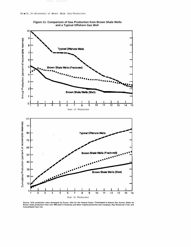
total recoverable reserves is produced in theearlier years of the life of the reservoir. [n figure11, the production profile of a typical offshore
50 ● Ch. VI—Economics of Brown Shale Gas Production
Figure 11. Comparison of Gas Production from Brown Shale Wellsand a Typical Offshore Gas Well
Year of Production
100 ‘
90 -
Year of Production
Source. OCS production rates developed by Exxon, USA for the Federal Power Commtswon’s Natural Gas Survey. Rates forBrown shale production from over 200 wells in Kentucky and West Vlrglnla (Columbla Gas Company, Ray Resources Corp, andConsolidated Gas Co).

Ch. Vi—Economics of Brown Shale Gas Product/on . 51
natural gas well is compared with those of two tion profile has a weaker positive effect upon thetypical Brown shale wells. In the first 15 years of ATNPV of the prospect. This production profile,production, only 38 to 54 percent of total together with the relatively small volume ofrecoverable shale gas reserves are produced, but reserves per unit of investment cost, has been theabout 85 percent of the reserves in the offshore principal reason that, until recently, Brown shalereservoir are produced. Production which is gas production has been economically sub-weighted toward the later years in the produc- marginal.
Cost and Technological Characteristics of
Brown Shale Production in Three Localities
Production data have been obtained from shot wells. These figures are the averages of ac-three gas-productive locations in the A p - tual production data for 13 wells in this field forpalachian Basin, These localities, in descending the 15-year period.order of general investment attractiveness, areCottageville, W.Va. (high quality); Clendenin,
In the medium-quality shale, data were availa-
W.Va. (medium quality); and Perry County, Ky.ble for both shot and hydrofractured wells, but
(lower quality). The quality designations reflectonly for 5 years. The rest of the profiles were ex-trapolated using production decline curves for
geologic and economic characteristics of eachBrown shale wells developed for the region.14
region and are not intended to reflect anydifferences in the actual Btu content of the lqBagnall and RYan, “The Geology, Reserves and Produc -natural gas in the fields. The 15-year production
tion Characteristics of the Devonian Shale in Southwesternprofiles are given in table 4. In the high-qual i ty West Virginia,” figure 11, Devonian Shale-Production andarea, production data were available only from Potentia/, ERDA, 1976.
Table 4Production Statistics of Natural Gas From Brown Shale in Three Localities
(Mcf Per Year)
Locales: High Quality Medium Quality Lower Quality
Good Bad
Stimulation: Shot Frac * Shot Frac Shot Frac Shot
Year-1 . . . . . . . . . . . . . . . . . . . . . . .23: : : : : : : : : : : : : : : : : : : : : : :4. .., . . . . . . . . . . . . . . . . . .5. ....., . . . . . . . . . . . . . . . .
36,31829,49023,88320,07117,43915,98014,87913,46412,77212,49811,66111,30411,13110,842
9,766
17,98920,22717,97818,57017,00016,00015,00014,50013,80013,50012,70012,20011,70011,30010,800
17,85816,05312,34211,00110,0009,0008,2007,5007,0006,5006,1005,8005,5005,2005,000
21,25020,85020,60017,70018,35017,29017,00016,30015,60015,00014,50013,80013,30012,80012,300
18,75015,88013,60011,4801-1,17011,08010,000
9,3008,7008,2007,8007,5007,2007,0006,800
11,40010,900
9,2009,6008,3007,5006,9006,3005,8005,0504,7504,5004,2504,0503,850
6,8005,0005,6005,1005,4005,3005,0004,9504,9004,8004,7004,6004,5504,4504,400
Source: Production and cost data on Brown shale operations are “Hydrofracturlng IS commonly referred to as “frac, ” which WIIIaverages from over 200 wells In Kentucky and West Vlrglnla (Co- be used as an abbreviation in tables In this report,Iumbla Gas Co., Ray Resources Corp., and Consolidated Gas).

52 . Ch. VI—Economics of Brown Shale Gas Production
Because of great, variability in the productionfrom the wells in the lower-quality location, thewells were separated into two groups-good andbad-based solely on their production rates.Shot and hydrofractured wells fell into bothgroups. Fifty-nine percent of the wells in thislocality fell into the good group, while the re-maining 41 percent were in the bad group. Onemight be misled by looking only at the goodgroups in this locality for comparison with thehigh- and medium-quality locality, because oneassumes a risk of having a bad well in this locality41 percent of the time. So, while one can get agood well from the lower-quality locality, the in--
vestment potential on average is less attractivethan in the other localities.
In judging the investment potential of thelocalities, there is concern regarding the costsassociated with the production: the initial costsfor drilling and stimulating the wells, the annualoperating costs, and the indirect cost from therisk of drilling a “dry hole. ” Table 5 shows theaverage of the direct initial costs for drilling and
Table 5Direct investment Costs for Producing
Wells in Brown Shale
(Dollars in thousands, 1976 constant)
Locality
High Quality . . . . . . .
Medium Quality . . . .
Lower Quality . . . . . . .
StimulationTechnique
Shot
FracShot
Frac
Shot
Locality
High Quality. . . . . . . . . .
Medium Quality . . . . . .
Lower Quality . . . . . . . .
Average Cost
In tan- Tan-gible gible
$ 80.5 $23.9
121.7 38.798.9 20.8
1 1 5 . 9 4 0 . 0
9 4 . 3 2 7 . 4
Total
$104.4
160.4119.7
155.9121.7
stimulating wells in the localities. The differencesin drilling costs reflect differences in depth of thewells in the various portions of the AppalachianBasin and in the drilling costs per foot, which area function of the geologic and topographiccharacteristics of the localities. Detailed costfigures are presented in tables 13 through 17 atthe end of this chapter.
Drilling costs in the lower-quality locality weretaken to be about $10 per foot, whereas theywere about $9 per foot in the other localities. It isrecognized that in some other areas these costsmay be as low as $6.50 per foot, but these areasare readily accessible and have easily workedgeologic formations. In light of the potential fortechnological advances in the drilling process, alow estimate is given in table 6, approximatelyreflecting a 10-percent reduction in actual drillingcosts .15 The effect of lower drilling costs or ofcheaper stimulation techniques on the invest-ment decision in the localities can be examinedby comparing the reduction in average and lowestimates with the ATNPV for the differentscenarios as displayed in tables 8 through 11.
The effect of progress in drilling technology orof improvement in stimulation procedures, whichreduces the initial investment cost per unit ofreserves, will be to extend the economicallyfeasible portion of the Devonian shale resource.A 10-percent decrease in real drilling costs, suchas that assumed for purposes of example in table6, would make some of the prospects in tables 8
I jsee, for exarrrple, Franklin M. Fisher, “Technological
C h a n g e a n d t h e D r i l l i n g C o s t - D e p t h R e l a t i o n s h i p ,1960 -66,” in E.W. Erickson and L. Waverman, editors, TheEnergy Question, Vol. 2, North America, University of Toron-to, 1974.
Table 6Effect of Reduction in Initial Investment Cost
(Dollars in thousands, 1976 constant)
StimulationTechnique
Change in ATNPVas a Result of
Average Cost Low Estimate Reduced Costs*
Shot $104.4 $ 90.4 +$6.5
FracShot
Frac
Shot
158.4 137,4 + 9 , 6119.7 102.6 + 7 . 8
155.9 144.3 + 5 . 3120.5 110.8 + 4 . 4
● The only change In tax effect considered IS In the first-year writeoff of lntanglble~.
Ch. VI—Economics of Bown Shale Gas Prodcution . 53
through 11, which have small negative ATNPVvalues, economically attractive.16
The average costs are separated into intangibleand tangible items because of the impact of thedifferent tax treatment as to expensing andcapitalizing these costs. The intangible costswere set to include a management fee of about15 percent and a contingency fee of 6 percent.While these figures may be high for some opera-tors at some locations, they are typical of currentcharges and are representative of anticipatedcosts if an extensive effort to develop the Brownshale should occur.
The annual operating costs are set at $1,800per well. While some operators may use a sub-stantially cheaper well-tending service, this figureprovides a cushion for expenses resulting fromequipment repair.
An additional cost to be considered is thatassociated with the risk of a “dry hole. ” This riskis difficult to assess because of the difficulty indetermining which wells are in fact “dry holes.”Of course, the clearest case is the hole whichproduces no natural gas at all. The problem ariseswhen there is some gas but the flow is not suffi-
I b s e n - l e of the wells w i th negat ive ATNPV values in ta-
bles 8-11 would nevertheless be producers because drillingcosts are already committed and the returns on incrementalout-of-pocket completion, stimulation and production costsare adequate to induce production. But these wells wouldnot return 10 percent after taxes on total Investment.
cient to make the well profitable based on itsown operations. The decision to continue thefinal casing of the well would be based on theadditional cost of finishing the well rather thanthe amount already invested. However, it is com-plicated not only by the uncertainty of the priceto be received for the gas but also by its useful-ness to the investors as a tax shelter for other in-come. In addition, under syndication, not only domarginal tax rates vary among investors andoperators, but which costs are sunk and whichare incremental may be different to investors andoperators. Hence, wel ls which would beeconomically unattractive on a total basis may bebrought into production for personal financialreasons of a key decisionmaker. This effect mayalso work in the opposite direction. Since it isalmost impossible to determine the impact ofthese incentives on the number of “dry holes, ”and some external incentives are likely to con-tinue to affect the “produce or plug” decision,the number of dry holes is taken to be thosewhich presently are not in actual productionregardless of the basis for the decision.
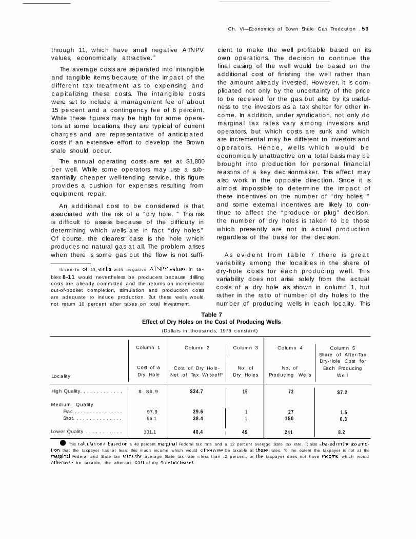
As evident f rom table 7 there is greatvariability among the localities in the share ofdry-hole costs for each producing well. Thisvariability does not arise solely from the actualcosts of a dry hole as shown in column 1, butrather in the ratio of number of dry holes to thenumber of producing wells in each locality. This
Table 7Effect of Dry Holes on the Cost of Producing Wells
(Dollars in thousands, 1976 constant)
Column 1
Cost of a
Locality Dry Hole
High Quality. . . . . . . . . . . . . $ 8 6 . 9
Medium QualityFrac . . . . . . . . . . . . . . . . 97.9Shot. . . . . . . . . . . . . . . 96.1
Lower Quality . . . . . . . . . . . 101.1
Column 2 I Column 3
ICost of Dry Hole- No. of
Net of Tax Writeoff* Dry Holes
$34.7 15
29.6 138.4 1
40.4 I 49
Column 4 Column 5Share of After-TaxDry-Hole Cost for
No, of Each ProducingProducing Wells Well
72 $7.2
27 1.5150 0.3
241 8.2
● This cal[ ulatlon I\ ba~ed on a 48 percent marginal Federal tax rate and a 12 percent average State tax rate. It also IS bawd on the assump-
tion that the taxpayer has at least this much income which would otherwise be taxable at the~e rates. To the extent the taxpayer is not at themarginal Federal and State tax rates, the average State tax rate IS less than 12 percent, or the taxpayer does not have Income which wouldotherwls~’ be taxable, the after-tax co~t of dry holes Increases
—.
54 . Ch. VI—Economics of Brown Shale Gas Production
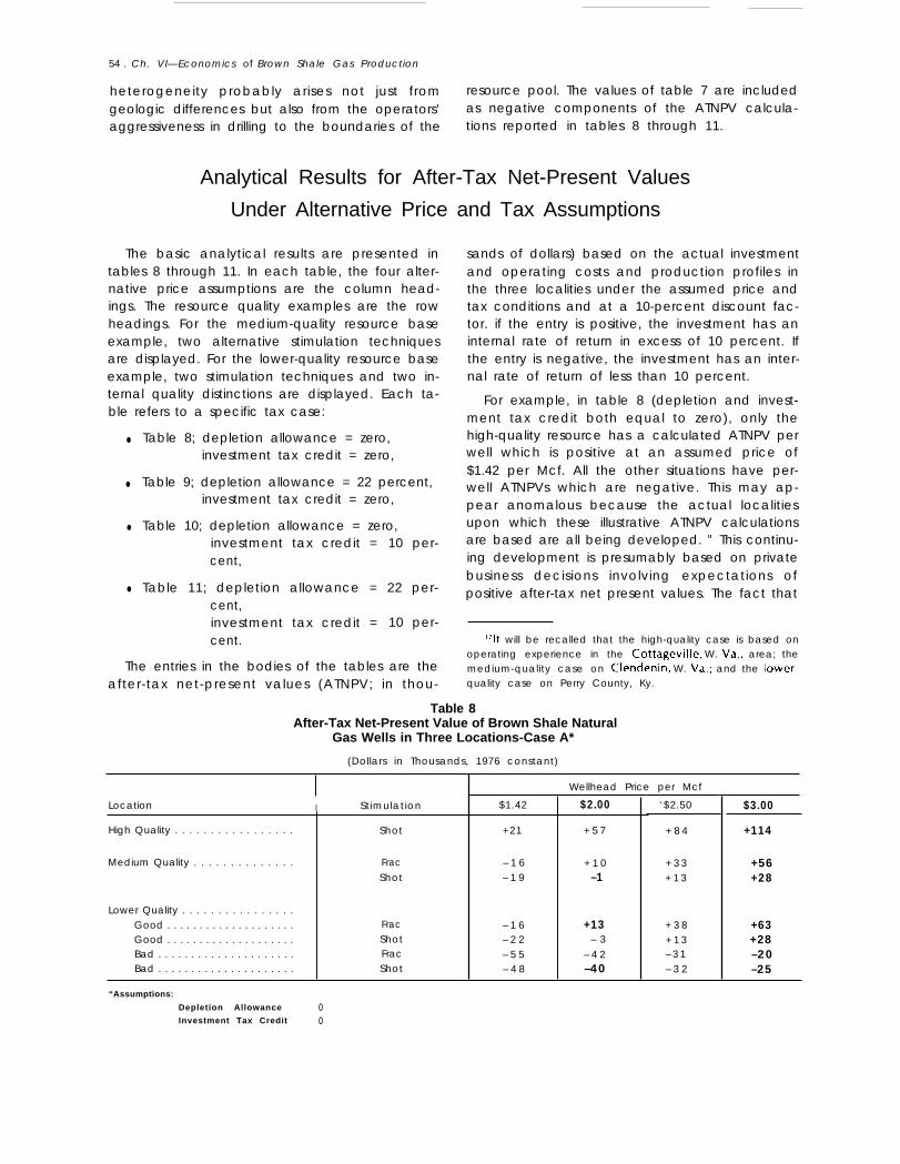
heterogeneity probably arises not just from resource pool. The values of table 7 are includedgeologic differences but also from the operators’ as negative components of the ATNPV calcula-aggressiveness in drilling to the boundaries of the tions reported in tables 8 through 11.
Analytical Results for After-Tax Net-Present Values
Under Alternative Price and Tax Assumptions
The basic analytical results are presented intables 8 through 11. In each table, the four alter-native price assumptions are the column head-ings. The resource quality examples are the rowheadings. For the medium-quality resource baseexample, two alternative stimulation techniquesare displayed. For the lower-quality resource baseexample, two stimulation techniques and two in-ternal quality distinctions are displayed. Each ta-ble refers to a specific tax case:
● Table 8; depletion allowance = zero,investment tax credit = zero,
● Table 9; depletion allowance = 22 percent,investment tax credit = zero,
● Table 10; depletion allowance = zero,investment tax credit = 10 per-cent,
● Table 11; depletion allowance = 22 per-cent,investment tax credit = 10 per-cent.
The entries in the bodies of the tables are theafter-tax net-present values (ATNPV; in thou-
sands of dollars) based on the actual investmentand operating costs and production profiles inthe three localities under the assumed price andtax conditions and at a 10-percent discount fac-tor. if the entry is positive, the investment has aninternal rate of return in excess of 10 percent. Ifthe entry is negative, the investment has an inter-nal rate of return of less than 10 percent.
For example, in table 8 (depletion and invest-ment tax credit both equal to zero), only thehigh-quality resource has a calculated ATNPV perwell which is positive at an assumed price of$1.42 per Mcf. All the other situations have per-well ATNPVs which are negative. This may ap-pear anomalous because the actual localitiesupon which these illustrative ATNPV calculationsare based are all being developed. ” This continu-ing development is presumably based on privatebusiness decisions involving expectations ofpositive after-tax net present values. The fact that
1“It will be recalled that the high-quality case is based onoperating experience in the Cottageville, W. Va., area; themedium-quality case on Clendenin, W. Va.; and the lower-quality case on Perry County, Ky.
Table 8After-Tax Net-Present Value of Brown Shale Natural
Gas Wells in Three Locations-Case A*
(Dollars in Thousands, 1976 constant)
Location I Stimulation
High Quality . . . . . . . . . . . . . . . . .
Medium Quality . . . . . . . . . . . . . .
Lower Quality . . . . . . . . . . . . . . . .Good . . . . . . . . . . . . . . . . . . . .Good . . . . . . . . . . . . . . . . . . . .Bad . . . . . . . . . . . . . . . . . . . . .Bad . . . . . . . . . . . . . . . . . . . . .
Shot
Frac
Shot
FracShotFracShot
$1.42
+21
– 1 6– 1 9
– 1 6– 2 2– 5 5– 4 8
Wellhead Price per Mcf
$2.00
+ 5 7
+ 1 0–1
+13– 3
– 4 2–40
‘$2.50
+ 8 4
+ 3 3+ 1 3
+ 3 8+ 1 3– 3 1– 3 2
$3.00
+114
+56+28
+63+28–20–25
“Assumptions:
Depletion Allowance oInvestment Tax Credit o

Ch. VI—Economics of Brown Shale Gas Production . 55
Table 9After-Tax Net-Present Value of Brown Shale Natural Gas Wells in Three Locations-Case B*
(Dollars in Thousands, 1976 constant)
Location
High Quality . . . . . . . . . . . . . . . . .
Medium Quality . . . . . . . . . . . .
Lower Quality
Good . . . . . . . . . . . . . . . . . . . .Good . . . . . . . . . . . . . . . . . . . .Bad . . . . . . . . . . . . . . . . . . . . .Bad . . . . . . . . . . . . . . . . . . . . .
Stimulation
Shot
FracShot
Frac
ShotFracShot
$1.42
+43
+1–8
+2– l o–50–45
Wellhead Price per Mcf
$2.00 I $2.50
+86
+34+14
+ 3 9+ 1 4–31–33
+ 1 2 3
+63+33
+70+35–17–23
$.3.00
+160
+91+51
+102+52–3
–13
● Asumptlons:
Depletion Allowance 220/0Investment Tax Credit o
Table 10After-Tax Net-Present Value of Brown Shale Natural Gas Wells in Three Locations-Case C*
(Dollars in Thousands, 1976 constant)
Locations I Stimulation
High Quality . . . . . . . . .“. . . . . . . .
Medium Quality . . . . . . . . . . . . . .
Lower QualityGood. . . . . . . . . . . . . . . . . . . .Good . . . . . . . . . . . . . . . . . . .Bad ., . . . . . . . . . . . . . . . . . . .Bad , . . . . . . . . . . . . . . . . . . . .
Shot
FracShot
FracShotFracShot
$1.42
+23 “
– 1 3– 1 7
– 1 3–20–52–46
Wellhead Price per Mcf
$2.00
+ 5 7
+ 1 3o
+16– 1– 3 9– 3 8
$2.50 I $3.00
+ 8 6 + 1 1 6
+ 3 6 + 5 9+ 1 5 +30
+41 +66+15 +32–28 –17–30 –23
“Assumption:
Depletion Allowance oInvestment Tax Credit 10“/0

56 . Ch. VI—Economics of Brown Shale Gas Production
Table 11After-Tax Net-Present Value of Brown Shale Natural Gas’ Wells in Three Locations-Case D*
(Dollars in Thousands, 1976 constant)
Location
High Quality ... . . . . . . . . . . . . .
Medium Quality . . . . . . . . . . . . . .
Lower QualityGood . . . . . . . . . . . . . . . . . . .Good . . . . . . . . . . . . . . . . . . . .Bad . . . . . . . . . . . . . . . . . . . . .Bad . . . . . . . . . . . . . . . . . . . .
● Assumption:
Stimulation
Shot
FracShot
FracShotFracShot
Depletion Allowance 220/0Investment Tax Credit 10“/0
the lower-limit base case has negative ATNPVSfor most situations is attributable to a number offactors:
●
●
●
●
●
there is no Btu adjustment in the assumedprices;
some of the gas is sold in intrastate marketsat higher prices;
the assumed tax treatment is more severethan that actually experienced by manyoperators;
the assumptions concerning investment andoperating costs and well Iives weregenerally slightly tilted in the direction ofadverse results; and
the poorer situations in the lower-qualityresource area are legitimate losers. “ “
The lower-limit base case for $1.42 per Mcf intable 8 reflects the conservative nature of theassumptions on which the ATNPV calculationsare based in all the price and tax cases analyzed.
The particular ATNPV figures reported intables 8 through 11 are all of interest,18 but what
Iqf economic incentives are such that there is substantial
Devonian shale development under conditions of positive
ATNPV per well, it can be expected that royalty payments,lease bonuses, and lease rentals will absorb the major por-tion of the difference between prospective expected
wellhead prices and costs.
$1 .42
+45
+4–6
+6–8
–46–43
Wellhead Price per Mcf
$2.00
+37
+37+16
+42+16–28–31
$2.50
+ 1 2 5
+ 6 6+ 3 4
+ 7 4+ 3 7– 1 3–21
$3.00
+162
+94+53
+105+58+1
–11
is of special interest is the general pattern ofresults. As the wellhead price of gas increasesfrom $1.42 per Mcf to $2.00 per Mcf, it becomeseconomically feasible to produce shale gas fromsome of the medium- and lower-quality sites ofthe gas-productive area. The price change of$1.42 per Mcf to $2.00 per Mcf appears to have agreater ef fect on making shale locat ionseconomically feasible than does the change from$2.00 to $2.50 per Mcf, or a change from $2.50to $3.00 per Mcf.
For example, in table 8, under the most severetax assumptions, at an assumed price of $2.00 perMcf, the pattern of ATNPV results is such that thehigh-quality resource area is a prime candidatefor development, the medium-quality resourcearea is marginally attractive, and the best situa-t ion in the lower-qual i ty resource area iseconomically rewarding. At $2.50 per Mcf, bothsituations in the medium-quality area becomeeconomically attractive and the good locations inthe lower-quality area have a positive ATNPV.Because the areal extent of each of these gas-productive quality areas is not known, the actualimpact on potential production cannot be deter-mined.
It is instructive to compare table 8 with table11. Table 8 is the most severe tax case examined.Table 11 is the most liberal (in terms of the
Ch. VI—Economics of Brown Shale Gas Production . 57
generosity with which income from gas produc-tion is treated) tax case examined. At $2.00 perMcf, two additional situations achieve positiveATNPV values in table 11 which did not achievepositive ATNPV values in table 8. These are shotwells in the medium-quality resource area andshot wells in the good area in the lower-qualityresource area. Note that the liberal tax treatmentdoes not increase the area of potential gas pro-duction, but does make shot wells economicallyfeasible in the medium- and lower-quality goodareas. A well head price of $2.50 per Mcf does notincrease the potentially productive area of theshale resource but it does increase the value ofthe wells and, like the $2.00 price, makes shotwells economically feasible. A wellhead price of$3.00 per Mcf under the most liberal tax treat-
ment makes shale gas production from all threelocalities in the gas-productive area economicallyfeasible.
A comparison of data in table 8 with that in ta-ble 9 shows that a 10-percent investment taxcredit would have little positive impact on shalegas development. However, a comparison of datain table 8 with that in table 10 shows the positiveimpact of a 22-percent depletion allowance. At$1.42 per Mcf, in addition to increasing the valueof wells in the high-quality locations, a 22-per-cent depletion allowance makes hydrofracturedwells in the medium- and lower-quality goodareas economically feasible. Basically, the 22-per-cent depletion allowance has about the samepositive effect as a $.50 per Mcf increase inwellhead price.
Extent of the Economically Producible
As indicated in an earlier section, estimates ofthe natural gas in the Brown shale are subject togreat variability. The question involves not onlythe total resource present but also the portionthat can be economically produced. Until theBrown shale resource of the Appalachian Basin ismore fully characterized, there will continue tobe great uncertainty in any attempt to estimatethe extent of the Appalachian Basin which mightsustain commercial development of shale gasproduction.
The ATNPV analyses indicate that under manyof the price and tax scenarios, drilling for andproducing shale gas from localities in the knownshale gas productive area is economically feasi-ble. However, it is unrealistic to assume that thecurrent gas-productive area is representative ofthe whole Appalachian Basin. A number ofgeneral observations about resource deposits arerelevant. First, the distribution of resourcedeposits in nature tend to be highly skewed, i.e.,there are fewer very high-quality resourcedeposits than medium-quality deposits, andfewer medium-quality deposits than low-quality
deposits.19, 20 Second,
Area
the better-quality resourcestend to be developed first.21 There being nostrong evidence to the contrary, OTA assumesthat these principles apply to gas-bearing shalesof the Appalachian Basin.
In a marginal resource base such as the Brownshale, the definition of “better-quality resource”includes, as a determinant, location relative toexisting production and pipelines. Until recently,the Brown shale have not been a primary target ofdrilling except in the Big Sandy area. The currentareas of shale development were initially
IYJ.W. McKie, “Market Structure and Uncertainty In Oiland Gas Exploration, ” Quarterly )ourna/ of Econom/cs, Vol.74, pp. 543-571, November, 1960.
20G. Kaufman, “Statistical Declslon and Related Tech-niques in Oi l and Gas Explorat ion, ’ Prent ice Hal l ,Englewood Cliffs, N. J., 1973, and J. Altchlson and J,A, C.Brown, “The Lognormal Distribution, ” Cambridge universityPress, New York, N. Y., 1957.
ZIC. Kaufman, Y. Bulcer, and D. Kryt. “A Probabilistic
Model of Oil and Gas Discovery, ” Studies In CeOIOgy, VOI.1, American Association of Petroleum Geologists, TUIM,Okla, pp. 113-142, 1975.

.58 . Ch. VI—Economics of Brown Shale Gas Production
byproducts of other activity. While it might ap-pear that this fact would blunt the operation ofthe principle that the better prospects are drilledfirst, this is not the case. Even if the initialknowledge of Brown shale prospects wasdeveloped as a byproduct of other activity, thebetter Brown shale prospects (byproducts or not)are developed first. “Better” here, however, in-volves a strong element of location relative to ex-isting pipelines. This is particularly true forhistorical wellhead price levels. Evidence of thisis that much of the Brown shale production inWest Virginia is served by existing interstatepipelines.
All of this suggests that there may be otherareas which are geologically as promising as thethree localities examined here. These other areas,although more remote relative to existingpipelines, may become economically feasible atthe $2.00 to $3.00 per Mcf price levels examinedin the sensitivity analysis reported herein.
There might be a temptation to extrapolate theproduction results from the three sample loca-tions in the currently productive, area directly tothe entire Appalachian Basin. Results of such anextrapolation are not likely to be valid primarilybecause:
● the existing wells are not located randomlyin the Appalachian Basin, but rather areclustered in a known producing area;
● the gas-productive area sampled (98.6square miles) is less than 0.06 percent of the163,000-square-mile Appalachian Basin;
● the 490 sample wells are but a very small (5percent) portion of the 10,000 producingwells in the Appalachian Basin, and do notrepresent a random sample; and
● average production data from producingwells are biased because dry holes andplugged and abandoned wells are not in-cluded in the “average production. ”
OTA assumed that the production potential inthe currently producing area is much higher thanis characteristic of the Appalachian Basin as awhole.
Based on the following information, OTA esti-mates that about 10 percent of the 163,000-square-mile extent of the Appalachian Basinmight be of high enough quality to produce shalegas economically at a price of $2.00 to $3.00 perMcf.
1.
2.
3.
Production History. —The wells which havea potential of producing more than 240 to300 Mcf of shale gas over a 15- to 20-yearperiod tend to be clustered in a few loca-tions in the Appalachian Basin. This type ofdistribution of commercially productivewells indicates that not all of the Ap-palachian Basin is composed of the sameresource quality. No doubt additional loca-tions exist which have commercial poten-tial, but it is unlikely that these areas willcomprise a significant portion of the163,000-square-mile extent of the Ap-palachian Basin.
Shale Depth. —The Brown shale outcrops atthe surface in central Ohio and is 12,000feet below the surface in northeastern Penn-sylvania. Because drilling and stimulationcosts increase with depth, commercial pro-duction of shale gas in the volumes encoun-tered in the best wells to date is generallylimited to depths less than 5,000 feet. Aconsiderable extent of the Brown shale ofthe Appalachian Basin is deeper than 5,000feet and is therefore unlikely to sustain com-mercial shale gas production under theeconomic conditions and technology con-sidered in this assessment.
Shale Thickness. —The total thickness of thegas-productive Brown shale sequence in theDevonian rocks varies from less than 100feet to more than 1,000 feet across the Ap-palachian Basin (figure 3). It is not generallyeconomical to stimulate Brown shale layerswhich are less than 100 feet in thicknessunless multiple layers in one well can betreated. The Brown shale resource in a sig-nificant portion of the Appalachian Basinconsists of thin layers of Brown shale whichmay not be amenable to modern hydrofrac-ture techniques.

Ch. VI—Economics of Brown Shale Gas Production ● 59
4 Fractures.—The fracture system (number, 5length, openness, and direction of fracturesor joints) in the Brown shale is not uniformacross the Appalachian Basin. The much-fractured areas of the Brown shale tend tobe more gas-productive than the less-frac-tured areas. Extensive areas of the Ap-palachian Basin have limited fracturesystems and therefore are potentially poorerareas for shale gas production even withmodern stimulation techniques than themuch-fractured areas.
Dril l ing Exper ience. -Dr i l l ing and pro-duction records of independent operators inthe Appalachian Basin have reflected vastareas where shale gas product ion i suneconomic unless new stimulation tech-niques can more than double shale gas pro-duction rates without significant increasesin cost. Poor shale gas production ex-perience over extensive areas probably is aresult of a combination of the circumstancesoutlined above.
An Estimate of Readily Recoverable
The Appalachian Basin has an areal extent ofabout 163,000 square miles. If 10 percent of thisarea is of high enough quality to be economicallyattractive for shale gas production at prices of
$2.00 to $3.00 per Mcf, it provides a potentialproduction area of 16,300 square miles. (Thepresent gas-productive area is less than 5 percentof the 163,000-square-mile area. ) With a spacingof 150 acres per well, this area would support ap-proximately 69,000 wells. Production data pre-sented in table 4 show that wells economicallyfeasible at $2.00 per Mcf will produce approx-imately 240 million cubic feet of shale gas perwell over a 15-year period, and about 290 millioncubic feet per well over 20 years.22 Readi lyrecoverable reserves were determined bymultiplying the number of potential wells by theaverage production per well as follows:
15-year readily recoverable reserve69,000 wells x 240 MMcf/well = 16.6 Tcf
20-year readily recoverable reserve69,000 wells x 290 MMcf/well = 20.0 Tcf
If the entire undeveloped gas-productive areawere a medium-quality resource and all wellswere shot treated, the 15-year readily recovera-ble reserve would be 9 Tcf; use of hydrofractur-ing rather than shot treatment would increase this
z~ln a Slmllar analysis for a smaller producing area, IJlti -
mate recoverable reserves were used at levels ot 300, 350,
and 400 MMcf per well, P. J, Brown, “Energy From Shale—ALittle Used Natural Resource. ” Natural Gas From Unconven-tional Geo/og/c Sources, National Academy of Sciences,J 976.
figure to 15 Tcf.reserves would
Reserves
The 20-year readily recoverableapproximate 11 and 19 Tcf,
respectively. If 10 percent of the 163,000-square-mile (1 6,300 square miles) gas-productive areawere all high-quality resource and all wells wereshot treated, the readily recoverable reservewould be about 17 Tcf over a 15-year period andabout 20 Tcf over a 20-year period. Assumingthat hydrofracturing results in a 50-percent in-crease in shale gas production (as is suggested byproduction data in table 4), 69,000 hydrofrac-tured wells on high-quality Brown shale sitesmight produce 26 Tcf of gas over a 15-yearperiod, and approximately 30 Tcf over a 20-yearperiod.
It is highly unlikely that all of the undevelopedgas-productive Brown shale resource will be highquality, and also unlikely that all of it will bemedium or low quality. For this reason, a 15 to 25Tct estimate of readily recoverable shale gasreserves appears justified until the Brown shaleresource base is more thoroughly characterized.This range clearly indicates that the Brown shaledo in fact have a potential for making a significantcontribution to the U.S. natural gas supply.
Because of the great uncertainty in the qualitydistribution of the shale resource, no attempt wasmade to undertake price elasticity studies in thisassessment. The impact of a specific price changeon shale gas production will be impossible toassess accurately until extensive resource charac-terization studies are completed, This will requirea large amount of drilling throughout the region.

60 • Ch VI—Economics of Brown Shale Gas Production
Some estimates of the total amount of gas-in-place in the Brown shale range in the hundreds ofTcf. 23 However, such estimates of the resourcebase should be distinguished from estimates ofreadily recoverable reserves, which represent thefraction of the total resource whose recovery isfeasible under reasonable assumptions about
costs, taxes, and geologic formations. OTA’s 15to 25 Tcf estimate of readily recoverable reservesis consistent with a total resource estimate ofhundreds of Tcf because of the fact that underpresent technology the average shale wellrecovers only 3 to 8 percent of the calculated gasin place .24
General Observations and Findings
it appears that under plausible economic,geologic, and technological assumptions, theBrown shale of the Appalachian Basin contain asmuch as 15 to 25 Tcf of readily25 recoverablenatural gas. This reserve would be producible inthe first 15 to 20 years of the production profileof typical reservoirs. Because one of the charac-teristics of Brown shale gas production is a slowflow rate over a very long period of time, ulti-mate recoverable reserves over the life of pro-duction would be greater. This 15 to 25 Tcf esti-mate critically depends on the price and costassumptions used, the total extent of the Brownshale resource, and the distributions of resourcequality.
The price assumptions ($2.00 to $3.00 perMcf) realistically reflect the current opportunityvalue of additions to the U.S. natural gas supplyand are consistent with general market condi-tions for both interstate and intrastate sales. Esti-mates of drilling, well completion, stimulation,and production costs are based on actual operat-ing experience.
The estimate of 15 to 25 Tcf of readilyrecoverable reserves is based on the assumptionthat about 10 percent of the 163,000-square-mileAppalachian Basin has Brown shale of highenough quality to permit the production of shalegas economically at prices of $2.00 to $3.00 perMcf.
~ ~~a~ura/ Gas From Unconventional Geologic Sources, p.
113, National Academy of Sciences, 1976.
~qlbid., p, 86.
Z5’’Readily recoverable reserves” is not a category in
either the American Gas Association or United StatesGeological Survey nomenclature. In the present context,“readily recoverable reserves” are resources which can beconverted to proved reserves and actually produced in a 15-to 20-year time frame.
From table 12 one sees the important role thatthe Brown shale could play in national natural gassupply, If annual production were at 1.0 Tcf,26 theregion would match some of the larger gas-pro-ducing States and make up almost 5 percent ofcurrent national production.
Table 12Estimated Gross Production of Natural Gasof the five Largest Producing States, 1976
I Gross ProductionState (Tcf/annum)
Texas ., ., . . . . . . . . . . . . . .Louisiana . . . . . . . . . . . . . . .Oklahoma . . . . . . . . . . . . . .New Mexico . . . . . . . . . . . .Kansas . . . . . . . . . . . . . . . . .
Total U.S. . . . . . . . . . .
7.77.11.81.20.8
20.9
Source: Gas Facts 1976, American Gas Association (1977), p. 24.
T h e e s t i m a t e s p r e s e n t e d in th is report arebased on the analysis of 490 producing wells inthree gas-productive localities. These 490 wellswere drilled by a large number of operators withdifferent financial situations and technicalcapabilities. There are some data available from asmaller number of wells drilled by a single opera-tor.27 If these single-operator data are, in fact,representative of the potential of the Brown shaleof the Appalachian Plateaus, this resource might
~bThe 1.() Tcf is a central estimate based on the 15 to 25
Tcf range; therefore, one should keep in mind the variabilityassociated with the point estimate.
~TK.1. Brooks, R.M. Forrest, and W.1. Morse, 1974. “Gas
Reserves in the Devoniain Shale in the Appalachian Basinthe Operating Territory of the Columbia Gas System. ”
(Mimeographed Report in the files of Columbia Gas SystemService Corporation, Columbus, Ohio.)

Ch. VI—Economics of Brown Shale Gas Production ● 61
account for more than 1.0 Tcf per year of addi-tional U.S. supply in the next 20 years. This largerproduction could result from either or both (1)greater average productivity per well, or (2) alarger resource base which would permit agreater number of wells of average productivity.However, even under an optimal combination ofcircumstances (1 5-percent higher average pro-duction per well and a 50-percent increase in theareal extent of the quality shale resource), onlyabout 30 to 35 Tcf of readily recoverable reserveswould be producible over 15 to 20 years. For thereasons cited previously, however, OTA con-siders such an optimal combination to beunlikely.
The 1.0 Tcf figure is a judgmental estimatebased on the facts that: (1) much potential shalegas production is likelyarea without immediatenections, and (2) a largequired to generate I S
recoverable reserves.
to spread over a wideaccess to pipeline con-amount of drilling is re-to 25 Tcf of readily
Based on production data from the threelocalities analyzed, creation of 15 to 25 Tcf ofreadily recoverable reserves will require drilling69,000 wells. In 1975, 38,498 wells were drilledin the United States.28 If drilling 69,000 wells withthe Appalachian Basin Brown shale as the targetpay zone were spread over 20 years, this numberof new wells would average 3,450 wells per year.This drilling alone would represent a 9-percent in-crease in drilling activity over the total U.S. 1976level. The U.S. drilling industry has shown con-s iderable abi l i ty to respond to increasedeconomic incentives. Between 1971 and 1975,total wells drilled increased by 45 percent (9 per-cent per year), from 26,532 to 38,498. Between197I and 1975, total rotary-drilling rigs in opera-tion increased by 70 percent (15 percent peryear), from 976 to 1,660. Because Brown shaleproduction is relatively well-intensive, andbecause it is likely to be scattered over extensiveareas, it is prudent to assume that shale gasdevelopment will proceed at a gradual pace,possibly spreading the required drilling effortover 15 to 20 years.
~~Dri I I i ng stati s t i e s a r e f r o m t h e 0// a n d Gas /ourna/,
Review and Forecast Issues, 1972 and 1976, pp. 91 and 114.
The fact that potential shale gas production islikely to be scattered over extensive areas con-tributes to a relatively slow pace of developmentbecause of the requirement that natural gas beshipped by pipelines. This suggests that theeconomically feasible expansion of the gas-pipeline network required to serve new shaledevelopment and production will be on an incre-mental basis. This in turn suggests that locationrelative to potential pipeline connections (in ad-dition to geologic promise) will continue to beanimportant determinant of the economic qualityof shale drilling prospects. As a result, gradualdevelopment is a prudent assumption.
The magnitude of the required drilling effortdoes, however, have an important aspect. Thedrilling of 3,450 wells per year in the AppalachianBasin would be a significant addition to total U.S.drilling activity. There has been an impressiverecord of technological progress in the U.S. drill-ing industry.29 This progress has been associatedwith deeper target horizons in the gulf coast andthe Southwest. It is possible that a drilling effortof the magnitude required to develop Brownshale gas resources would sufficiently focus theattention of the drilling industry so that substan-tial technological progress in reducing shale drill-ing costs and improved deliverability wouldresult. A comparison of table 6 with tables 8through 11 indicates the potential of suchprogress to extend the margin of economicfeasibility for Brown shale development. Thepossibility of improved drilling and completiontechnology is not included in the 15 to 25 Tcfestimate.
The comparison of table 6 with tables 8through 11 is relevant to any technological ad-vance which improves the ratio of productivecapacity to investment cost, All Brown shale gasproduction is artif icially stimulated througheither hydrofracturing or shooting.30 An improve-ment in stimulation technology would have aneffect similar to that of an improvement in drill-ing technology. The possibility of an improve-ment in stimulation technology is not included inthe 15 to 25 Tcf estimate.
%ee FM. Fisher, o p c It.IO It i s n o t e w o r t h y t h a t hydrofracturlng i t s e l f w a s
developed in response to the post World War II Increase inU.S. crude oil prices,
62 . Ch. VI—Economics of Brown Shale Gas Production
If improvements in drilling or stimulation tech-nology are developed by drilling or well-servicecontractors who can patent the techniques, it ispossible that the socially optimal amount ofeffort to develop such technology wil l beforthcoming. But it is likely that much drilling,well stimulation, and production will be done byoperators who do not have a very large share oftotal shale production. In addition, many techni-cal improvements may not be readily patentable.Under these circumstances, the Congress maywish to consider the desirability of some publiclysupported research and development activitydirected toward improvements in shale drillingand stimulation technology.
The possible effect of either (1) dramaticallyimproved technology, or (2) improvements ineconomic incentives beyond those examinedhere, must be considered with caution. This isbecause of the likelihood that the developmenteffort which such possibilities would encouragewould be working against an increasinglymarginal resource base. If economic incentiveswere to be twice as good as those associatedwith current tax treatment and wellhead prices of$2.00 to $3.00 per Mcf; or, alternatively, if drill-ing and stimulation technology were to improveso that these operations cost only half as much asthey do now, it is unlikely that twice as great aquantity of reserves would become economicallyfeasible. This is because the additional develop-ment efforts which such economic or technologi-cal improvements would induce would be press-ing further and further into the margin of poorerand poorer sites and geologic prospects. In addi-tion, because poorer resource quality in theBrown shale is very much associated with slowerflow rates per unit of ultimately recoverablereserves, the contribution to yearly output wouldbe apt to increase relatively less than the increasein reserves. For example, on a purely illustrativebasis, if a doubling of economic incentives ortechnical productivity were to result in a 50-per-
cent increase in ultimate recovery, average out-put in the first 20 years might increase by only 25percent.
The 15 to 25 Tcf of readily recoverablereserves and approximately 1.0 Tcf of yearly pro-duction reported here are based on the followingassumptions:
●
●
●
●
●
It is
no significant changes in real drilling, wellstimulation, or production costs;
the economic and production charac-teristics of the three localities analyzedrepresent the more promising sources ofnatural gas from the Brown shale;
wellhead prices for natural gas in the $2.00to $3.00 per Mcf range;
continuation of current tax treatment of in-come from natural gas production; and
approximately 10 percent of total now un-developed Appalachian Basin Brown shaleresource is of high enough quality to permitcommercial development.
a well-known axiom that there is no sureproof of gas or oil production potential otherthan the drillbit. It is possible that all of theundrilled resource potential of the Devonianshale has economic and production charac-teristics similar to those of the bad situations inthe lower-quality resource area. In this case, therewould be no incremental Brown shale gas pro-duction which would be economically feasible,at wellhead prices in the range of $2.00 to $2.50per Mcf. This appears unl ikely, given thegeographic dispersion of Brown shale resources.There appears to be no practical way short ofcreating the economic incentives necessary to in-duce an extensive drilling effort, to ascertainwhether the Appalachian Basin shale might ac-tually contribute more, or less, than 5 percent ofthe total U.S. natural gas supply.

Table 13Typical Well Costs (1976 Constant Dollars)
High-Quality Brown Shale Well
Cottageville Area, Jackson County, W.Va.
Total Depth-4,300 feet
Completion Method-Shooting 450 feet of Gross Pay Section
Intangible Costs:Title work . . . . . . . . . . . . . . . . . . .Stake Iocation. . . . . . . . . . . . . . . .Drilling permit & bond . . . . . . . . .Other legal expenses. ... . . . . . .Right-of-way expenses. . . . . . . . . .Road & location costs . . . . . . .Hauling (all except cement) . . . . .Well logs (open hole) . . . . . . . . . .Centralizers & float equipment . .Cementing surface & conductor .Shooting 450 feet . . . . . . . . . . . .Geologic & engineering service . .Drilling 4,200 feet @ $8/ft . . . . . .Rig charges . . . . . . . . . . . . . . . . . . .Install 2,000 feet flow line . . . . . .Reclaim road & location ., . . . . . .
S u b t o t a l . . . .
Contingency (6% of intangibles) .Management overhead (1 50/0 total
well costs excluding contingen-cy) . . . . . . . . . . . . . . . . . .
Total Intangibles ., . . . . . .Tangible Costs:Conductor casing:
30 feet of 13“@$l4.45/ft . .500 feet of 9-5/8 ’’@$9 .36/ft, .2,500 feet of 7“@$5.96/ft. . . .
Christmas tree. . . . . . . . . . . . . . .Valves & fittings. . . . . . . . . . . . . . .2,000’ of 2-3/8” flow line
@$.91/ft. . . . . . . . . . . . . . . . . . .Total Tangibles . . . . . . . . . .
Total Well Costs . . . . . . . .
ProducingWell
$ 300300350200100
2,0003,5003,0001,8003,5005,0002,800
34,4002,6001,7302,000
63,580
3,815
13,11580,510
4304,700
14,9001,0001,000
1,82023,850
$104,360
DryHole
$ 300300350200—
2,0003,5003,0001,8003,500
—1,400
34,400——
2,00052,750
3,165
10,91766,832
4304,700
14,900——
—20,030
186,862
Ch VI—Economics of Brown Shale Gas Producation • 63
Table 14Typical Well Costs (1976 Constant Dollars)
Medium-Quality Brown Shale Well
Blue Creek Area, Kanawha Co., W.Va.
Total Depth-500 feetCompletion Method-Hydrofracture (1,000 bbl)
Intangible Costs:Title work . . . . . . . . . . . . . . ., . .
Stake location. . . . . . . . . . . . . . . . .
Well permit & bond . . . . . . . . . . .Other legal expenses. , . . . . . . . . .Right-of-way expenses, . . . . . . . . .Road & location costs . . . . . . . . .Hauling (all except cement &
4-1/2” casing) . . . . . . . . . . .Hauling 4-1 /2” casing & line . . . .Well logs (open hole) . . . . . . . . . .Centralizers & float equipment . .Cementing conductor & surface .Cementing 4-1 /2” casing . . . . . .Hydrofrac-1,000 bbl, 60,000# sd,
75,000 cu. ft. nitrogen . . . . . . . .Perforate & CBL log . . . . . . . . . . .Tool and equipment rental . . . . . .Frac tank rental (5 x 250-
bbl@$l50/tank) . . . . . . . . . . . . . .Pump or haul water @
40/bbl x 1,000 . . . . . . . . . . . . . . . .
Completion rig 140 hrs@ $55/hr .Geologic & engineering service . .Drilling 5,000 feet @ $9/ft . . . . . .Rig charges . . . . . . . . . . . . . . . . . . .Install 2,000 feet flow line . . . . . .Reclaim road & location . . . . . . .
Subtotal . . . . . . . . . . . . . .
Contingency (6°/0 of intangibles) .Management overhead (1 50/0 of
total well costs excluding con-tingencies) . . . . . . . . . . . . . . . . .
Total Intangibles . . . . . . . . .
Tangible Costs:Conductor casing:
30 feet of 13“ @ $14.45/ft, . .500 feet of 9-5/8” @ $9.36/ft2,000 feet of 7“ @ $5.96/ft . .
Production casing: 5000 feet of4-1 /2” @ $3.12/ft . . . . .
Christmas tree. . . . . . . . . . . . . . . . .Valves & fittings. . . . . . . . . . . . . . .2,000 feet of 2-3/8” flow line
@$.91/’ft . . . . . . . . . . . . . . . . . . . .Separator & tank ., . . . . . . . .Valves & fittings, drips . . . . . . . .
Total Tangibles . . . . . . . . .
Total L ine & Wel l Costs
ProducingWell
$ 300350350200100
4,000
3,500520
3,2001,8003,5003,300
9,020,2,000
500
750
4007,7003,000
45,0002,6001,7302,000
95,820
5,749
20,176121,745
4304,700
11,900
15,6001,0001,000
1,8202,000
23538,685
$160,430
DryHole
$ 300350350200
—4,000
3,500—
3,2001,800.3,500
—
———
—
——
50045,000
——
2,00064,700
3,882
12,26080,842
4304,700
11,900
———
———
17,030
97,872
64 Ž Ch. VI—Economics of Brown Shale Gas Production
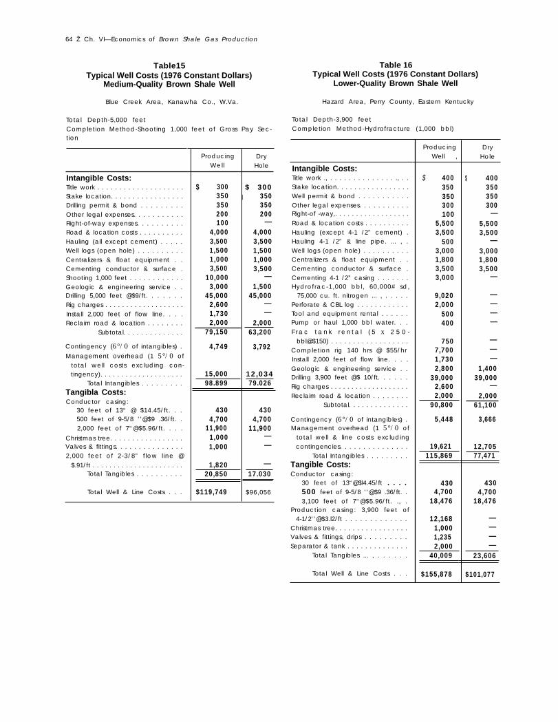
Table15Typical Well Costs (1976 Constant Dollars)
Medium-Quality Brown Shale Well
Blue Creek Area, Kanawha Co., W.Va.
Total Depth-5,000 feetCompletion Method-Shooting 1,000 feet of Gross Pay Sec-
Table 16Typical Well Costs (1976 Constant Dollars)
Lower-Quality Brown Shale Well
Hazard Area, Perry County, Eastern Kentucky
Total Depth-3,900 feetCompletion Method-Hydrofracture (1,000 bbl)
tion
Intangible Costs:Title work . . . . . . . . . . . . . . . . . . . .Stake location. . . . . . . . . . . . . . . . .Drilling permit & bond . . . . . . . . .Other legal expenses. . . . . . . . . . .Right-of-way expenses. . . . . . . . . .Road & location costs . . . . . . . . . .Hauling (all except cement) . . . . .Well logs (open hole) . . . . . . . . . .Centralizers & float equipment . .Cementing conductor & surface .Shooting 1,000 feet . . . . . . . . . . . .Geologic & engineering service . .Drilling 5,000 feet @$9/ft. . . . . . .Rig charges . . . . . . . . . . . . . . . . . . .Install 2,000 feet of flow line. . . .Reclaim road & location . . . . . . . .
Subtotal. . . . . . . . . . . . . .
Contingency (6°/0 of intangibles) .
Management overhead (1 5°/0 oftotal well costs excluding con-tingency). . . . . . . . . . . . . . . . . . . .
Total Intangibles . . . . . . . . .
Tangibla Costs:Conductor casing:
30 feet of 13“ @ $14.45/ft. . .500 feet of 9-5/8 ’’@$9 .36/ft. .2,000 feet of 7“@$5.96/ft. . . .
Christmas tree. . . . . . . . . . . . . . . . .Valves & fittings. . . . . . . . . . . . . . .2,000 feet of 2-3/8” flow line @
$.91/ft . . . . . . . . . . . . . . . . . . . . . .Total Tangibles . . . . . . . . . .
Total Well & Line Costs . . .
ProducingWell
$ 300350 I350200100
4,0003,5001,5001,0003,500
10,0003,000
45,0002,6001,7302,000
79,150
4,749
15,00098.899
4304,700
11,9001,0001,000
1,82020,850
$119,749
DryHole
$ 300350350200—
4,0003,5001,5001,0003,500
—1,500
45,000——
2,00063,200
3,792
12,03479.026
4304,700
11,900——
—17.030
$96,056
Intangible Costs:Title work ., . . . . . . . . . . . . . . ., . .Stake location. . . . . . . . . . . . . . . . .Well permit & bond . . . . . . . . . . .Other legal expenses. . . . . . . . . . .Right-of -way,. . . . . . . . . . . . . . . . . .
Road & location costs . . . . . . . . . .Hauling (except 4-1 /2” cement) .Hauling 4-1 /2” & line pipe. ... , .Well logs (open hole) . . . . . . . . . .Centralizers & float equipment . .Cementing conductor & surface .Cementing 4-1 /2” casing . . . . . . .Hydrofrac-1,000 bbl, 60,000# sd,
75,000 cu. ft. nitrogen ... , . . . . .Perforate & CBL log . . . . . . . . . . . .Tool and equipment rental . . . . . .Pump or haul 1,000 bbl water. . .
F r a c t a n k r e n t a l ( 5 x 2 5 0 -bbl@$150) . . . . . . . . . . . . . . . . . .
Completion rig 140 hrs @ $55/hrInstall 2,000 feet of flow line. . . .
Geologic & engineering service . .Drilling 3,900 feet @$ 10/ft. . . . . .Rig charges . . . . . . . . . . . . . . . . . . .Reclaim road & location . . . . . . . .
Subtotal. . . . . . . . . . . . . .
Contingency (6°/0 of intangibles) .Management overhead (1 5°/0 of
total well & line costs excludingcontingencies. . . . . . . . . . . . . . .
Total Intangibles . . . . . . . . .Tangible Costs:Conductor casing:
30 feet of 13“@$l4.45/ft . . . .500 feet of 9-5/8 ’’@$9 .36/ft. .3,100 feet of 7“@$5.96/ft. ., .
Production casing: 3,900 feet of4-1/2’’@$3.l2/ft . . . . . . . . . . . . .
Christmas tree. . . . . . . . . . . . . . . . .Valves & fittings, drips . . . . . . . . .Separator & tank . . . . . . . . . . . . . .
Total Tangibles ... , . . . . . .
Total Well & Line Costs . . .
ProducingWell ,
$ 400350350300100
5,5003,500
5003,0001,8003,5003,000
9,0202,000
500400
7507,7001,7302,800
39,0002,6002,000
90,800
5,448
19,621115,869
4304,700
18,476
12,1681,0001,2352,000
40,009
$155,878
DryHole
$ 400350350300—
5,5003,500
—3,0001,8003,500
—
————
———
1,40039,000
—2,000
61,100
3,666
12,70577,471
4304,700
18,476
————
23,606
$101,077
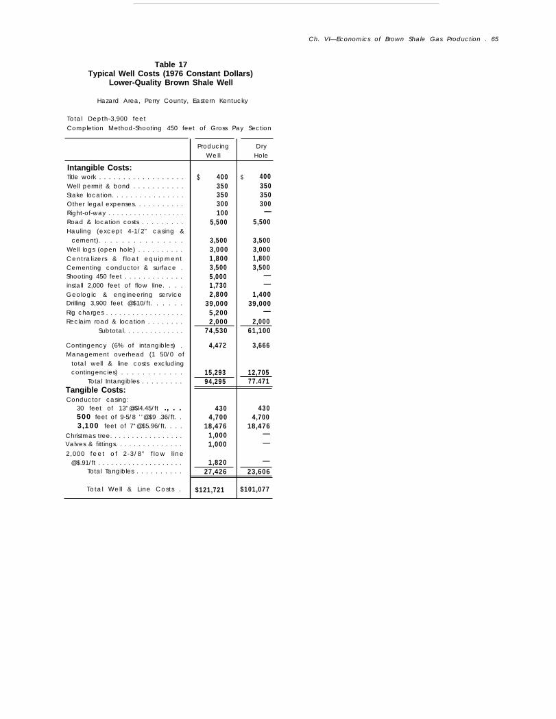
Ch. VI—Economics of Brown Shale Gas Production . 65
Table 17Typical Well Costs (1976 Constant Dollars)
Lower-Quality Brown Shale Well
Hazard Area, Perry County, Eastern Kentucky
Total Depth-3,900 feet
Completion Method-Shooting 450 feet of Gross Pay Section
Intangible Costs:Title work . . . . . . . . . . . . . . . . . .Well permit & bond . . . . . . . . . . .Stake location. . . . . . . . . . . . . . . .Other legal expenses. . . . . . . . . . .Right-of-way . . . . . . . . . . . . . . . . . .Road & location costs . . . . . . . . .Hauling (except 4-1/2” casing &
cement). . . . . . . . . . . . . . .Well logs (open hole) . . . . . . . . . .Centralizers & float equipmentCementing conductor & surface .Shooting 450 feet . . . . . . . . . . . . .install 2,000 feet of flow line. . . .Geologic & engineering serviceDrilling 3,900 feet @$10/ft. . . . . .
Rig charges . . . . . . . . . . . . . . . . . .Reclaim road & location . . . . . . . .
Subtotal. . . . . . . . . . . . . .
Contingency (6% of intangibles) .Management overhead (1 50/0 of
total well & line costs excludingcontingencies) . . . . . . . . . . . .
Total Intangibles . . . . . . . . .Tangible Costs:Conductor casing:
30 feet of 13“@$l4.45/ft ., . .500 feet of 9-5/8 ’’@$9 .36/ft. .3,100 feet of 7“@$5.96/ft. . . .
Christmas tree. . . . . . . . . . . . . . . . .Valves & fittings. . . . . . . . . . . . . . .
2,000 feet of 2-3/8” f low l ine@$.91/ft . . . . . . . . . . . . . . . . . . . .
Total Tangibles . . . . . . . . . .
Total Well & Line Costs .
ProducingWell
$ 400350350300100
5,500
3,5003,0001,8003,5005,0001,7302,800
39,0005,2002,000
74,530
4,472
15,29394,295
4304,700
18,4761,0001,000
1,82027,426
$121,721
DryHole
$ 400350350300—
5,500
3,5003,0001,8003,500
——
1,40039,000
—2,000
61,100
3,666
12,70577.471
4304,700
18,476——
—23,606
$101,077