VHE Emission from TeV J2032+4130

and Iterative Deconvolution in

Ground Based Gamma-ray

Astronomy

Gary E. Kenny B.Sc.

Thesis submitted to the National University of Ireland, Galway

for the award of Ph.D in the

Department of Physics

Supervisor: Dr. M. Lang

Co-Supervisor: Dr. G. Gillanders

September 2007

For Helena & Hannah Beth

Abstract

This thesis describes an investigation of Very High Energy (VHE) γ-ray

emission from the unidentified γ-ray source TeV J2032+4130. The analysis

was based on archival data from the 1989-1990 observing seasons obtained

using the Whipple 10-metre imaging atmospheric Cherenkov telescope in

southern Arizona. Fifty hours of data were analysed using the standard

Supercuts criteria, a set of optimised energy dependent parameter cuts, and

the application of the multivariate Kernel analysis method. On the basis

of detailed simulations of the detector, the VHE flux of TeV J2032+4130,

above 1 TeV, was determined to be (1.3 ±0.4 ±0.5) × 10−8 m−2s−1. This

corresponds to ∼ 6.2% of the flux of the Crab Nebula and suggests the source

is steady over a decade long interval.

An investigation into the effect of iteratively deconvolving the telescope

point spread function from atmospheric Cherenkov images was also carried

out. The Richardson - Lucy algorithm was used along with the measured

point spread function of the instrument to sharpen images in an attempt to

enhance our ability to discriminate against background Cosmic ray events.

The improvement in signal using this method was not statistically significant.

Also reported is the development of a semi-automated alignment system for

aligning the mirror facets of the telescopes of the new VERITAS array.

Contents

Key to Abbreviations xix

Acknowledgements xx

1 A Brief History of γ-ray Astrophysics and Thesis Overview 1

1.1 Introduction . . . . . . . . . . . . . . . . . . . . . . . . . . . . 1

1.2 Early Balloon and Space-based Experiments . . . . . . . . . . 3

1.3 Advances in Ground-Based Techniques . . . . . . . . . . . . . 4

1.4 Modern Satellite γ-ray Astronomy . . . . . . . . . . . . . . . . 5

1.4.1 The Compton Gamma Ray Observatory . . . . . . . . 5

1.4.2 Next Generation Satellite Experiments . . . . . . . . . 6

1.5 Thesis Overview . . . . . . . . . . . . . . . . . . . . . . . . . . 9

1.6 Contributory Summary . . . . . . . . . . . . . . . . . . . . . . 11

2 Ground-Based γ-ray Astronomy & the Imaging Atmospheric

Cherenkov Technique 13

2.1 Introduction . . . . . . . . . . . . . . . . . . . . . . . . . . . . 13

2.2 The High Energy Universe . . . . . . . . . . . . . . . . . . . . 14

2.3 Astrophysical Production Mechanisms of TeV γ-rays. . . . . . 17

2.3.1 Acceleration of Charged particles . . . . . . . . . . . . 18

2.3.2 Particle Decay . . . . . . . . . . . . . . . . . . . . . . . 24

i

2.4 The Imaging Atmospheric Cherenkov Technique . . . . . . . . 24

2.5 Cherenkov Radiation . . . . . . . . . . . . . . . . . . . . . . . 26

2.5.1 Introduction . . . . . . . . . . . . . . . . . . . . . . . . 26

2.5.2 Cherenkov radiation production . . . . . . . . . . . . . 27

2.6 Extensive Air Showers . . . . . . . . . . . . . . . . . . . . . . 29

2.6.1 Electromagnetic Air Showers . . . . . . . . . . . . . . . 29

2.6.2 Hadronic Air Showers . . . . . . . . . . . . . . . . . . 31

2.7 Discrimination between hadronic and γ-ray initiated EAS . . . 34

2.7.1 Detecting Cherenkov Radiation . . . . . . . . . . . . . 38

3 The Whipple 10 m Telescope 41

3.1 Introduction . . . . . . . . . . . . . . . . . . . . . . . . . . . . 41

3.1.1 Davies-Cotton Reflector Design . . . . . . . . . . . . . 42

3.2 Camera . . . . . . . . . . . . . . . . . . . . . . . . . . . . . . 45

3.2.1 Camera development . . . . . . . . . . . . . . . . . . . 49

3.3 Data Acquisition System . . . . . . . . . . . . . . . . . . . . . 50

3.3.1 Amplification . . . . . . . . . . . . . . . . . . . . . . . 50

3.3.2 Multiplicity Trigger . . . . . . . . . . . . . . . . . . . . 53

3.3.3 Pattern Selection Trigger . . . . . . . . . . . . . . . . . 53

3.3.4 Pedestal Trigger . . . . . . . . . . . . . . . . . . . . . . 55

3.3.5 Data Read out and Recording . . . . . . . . . . . . . . 56

3.4 Data Analysis Techniques . . . . . . . . . . . . . . . . . . . . 57

3.4.1 Data Calibration . . . . . . . . . . . . . . . . . . . . . 57

3.4.2 Standard Image Analysis (Supercuts) . . . . . . . . . . 60

3.4.3 Kernel Analysis . . . . . . . . . . . . . . . . . . . . . . 62

3.5 Observations and Operation . . . . . . . . . . . . . . . . . . . 66

3.6 Monitoring . . . . . . . . . . . . . . . . . . . . . . . . . . . . . 70

3.6.1 Timing . . . . . . . . . . . . . . . . . . . . . . . . . . . 70

ii

3.6.2 Tracking . . . . . . . . . . . . . . . . . . . . . . . . . . 71

3.6.3 Nitrogen Lamp . . . . . . . . . . . . . . . . . . . . . . 72

3.6.4 High Voltage System . . . . . . . . . . . . . . . . . . . 72

3.6.5 Current Monitor . . . . . . . . . . . . . . . . . . . . . 72

3.6.6 Weather Monitoring . . . . . . . . . . . . . . . . . . . 73

4 VHE γ-ray Sources and Ground Based Detectors 75

4.1 VHE γ-ray Sources . . . . . . . . . . . . . . . . . . . . . . . . 75

4.1.1 Supernova Remnants . . . . . . . . . . . . . . . . . . . 76

4.1.2 Other SNR Detections . . . . . . . . . . . . . . . . . . 86

4.1.3 Unidentified sources . . . . . . . . . . . . . . . . . . . 90

4.1.4 Dark Accelerators . . . . . . . . . . . . . . . . . . . . . 93

4.1.5 Other Sources of TeV γ-rays . . . . . . . . . . . . . . . 94

4.2 Major Imaging Atmospheric Cherenkov Experiments . . . . . 97

4.2.1 HESS . . . . . . . . . . . . . . . . . . . . . . . . . . . 98

4.2.2 The VERITAS Collaboration . . . . . . . . . . . . . . 99

4.2.3 MAGIC . . . . . . . . . . . . . . . . . . . . . . . . . . 101

4.2.4 CANGAROO-III . . . . . . . . . . . . . . . . . . . . . 102

4.3 The Milagro Detector . . . . . . . . . . . . . . . . . . . . . . . 103

4.4 Summary . . . . . . . . . . . . . . . . . . . . . . . . . . . . . 104

5 VERITAS Reflector Alignment and Point Spread Function.106

5.1 Introduction . . . . . . . . . . . . . . . . . . . . . . . . . . . . 106

5.2 Point Spread Function . . . . . . . . . . . . . . . . . . . . . . 109

5.3 Optical Alignment . . . . . . . . . . . . . . . . . . . . . . . . 112

5.3.1 Manual Alignment Procedure . . . . . . . . . . . . . . 115

5.3.2 Semi-Automated Alignment System . . . . . . . . . . . 117

5.3.3 System description . . . . . . . . . . . . . . . . . . . . 118

iii

5.3.4 Calibration . . . . . . . . . . . . . . . . . . . . . . . . 119

5.3.5 Semi-automated Alignment Procedure . . . . . . . . . 120

5.4 Results . . . . . . . . . . . . . . . . . . . . . . . . . . . . . . . 121

5.4.1 PSF of the VERITAS telescopes . . . . . . . . . . . . . 121

5.5 Bias Alignment . . . . . . . . . . . . . . . . . . . . . . . . . . 123

6 Iterative Deconvolution of Whipple Cherenkov Data 126

6.1 Introduction . . . . . . . . . . . . . . . . . . . . . . . . . . . . 126

6.2 Richardson - Lucy algorithm . . . . . . . . . . . . . . . . . . . 127

6.3 Algorithm Development . . . . . . . . . . . . . . . . . . . . . 131

6.3.1 Testing the algorithm . . . . . . . . . . . . . . . . . . . 134

6.4 Observations and Analysis . . . . . . . . . . . . . . . . . . . . 138

6.4.1 Picture and Boundary thresholds . . . . . . . . . . . . 140

6.4.2 Cut Optimisation . . . . . . . . . . . . . . . . . . . . . 142

6.5 Results . . . . . . . . . . . . . . . . . . . . . . . . . . . . . . . 143

6.6 Conclusions . . . . . . . . . . . . . . . . . . . . . . . . . . . . 144

7 Reanalysis of archival data of the unidentified TeV source

TeV J2032+4130 148

7.1 Introduction . . . . . . . . . . . . . . . . . . . . . . . . . . . . 148

7.2 Observations . . . . . . . . . . . . . . . . . . . . . . . . . . . . 149

7.3 Supercuts Optimisation . . . . . . . . . . . . . . . . . . . . . . 152

7.3.1 Background . . . . . . . . . . . . . . . . . . . . . . . . 152

7.3.2 Optimisation Method and Results . . . . . . . . . . . . 156

7.4 Energy-Dependent Cuts . . . . . . . . . . . . . . . . . . . . . 157

7.4.1 Energy-Dependent Cuts Results . . . . . . . . . . . . . 163

7.4.2 Gamma-Ray Simulations . . . . . . . . . . . . . . . . . 165

iv

7.4.3 Simulations for off-axis sensitivity of the 109 PMT

Whipple Camera . . . . . . . . . . . . . . . . . . . . . 167

7.5 The Kernel Analysis Method . . . . . . . . . . . . . . . . . . 174

7.6 Kernel Results . . . . . . . . . . . . . . . . . . . . . . . . . . . 175

7.6.1 Pre-Selection . . . . . . . . . . . . . . . . . . . . . . . 175

7.6.2 Kernel Cut Optimisation . . . . . . . . . . . . . . . . . 175

7.7 Energy Threshold and Flux Calculation . . . . . . . . . . . . . 178

8 Discussion 185

8.1 Summary of Work . . . . . . . . . . . . . . . . . . . . . . . . 185

8.2 Flux Determination of TeV J2032+4130 . . . . . . . . . . . . 187

8.3 Science Discussion . . . . . . . . . . . . . . . . . . . . . . . . 188

8.4 Conclusions . . . . . . . . . . . . . . . . . . . . . . . . . . . . 200

8.5 Future Possibilities in Ground Based γ-ray Astronomy . . . . 203

A Hillas parameters 207

B Publications List 210

C Data files used 224

References 242

v

List of Figures

1.1 Catalogue of sources detected by EGRET during its lifetime

including unidentified sources, pulsars, AGN and low confi-

dence identifications with AGN. Figure from Fegan (2003). . 7

1.2 The Gamma-ray Large Area Space Telescope (GLAST). The

top section of the spacecraft contains the LAT instrument and

the lower section contains the GBM. See text for more details.

Figure from NASA (education and public outreach). . . . . . . 8

2.1 A representation of synchrotron radiation production. As the

electron spirals along a magnetic field line, a cone of syn-

chrotron radiation is emitted at a tangent to the electron’s

trajectory. . . . . . . . . . . . . . . . . . . . . . . . . . . . . . 19

2.2 Frequency distribution of synchrotron electrons showing the

characteristic peak emission near 0.29νc where νc is the critical

frequency as defined in Equation 2.1 . . . . . . . . . . . . . . 21

2.3 A representation of Inverse-Compton Scattering. . . . . . . . . 22

2.4 The Crab Nebula supernova remnant observed with the Hub-

ble Space Telescope. Figure courtesy of the Hubble Heritage

Team (heritage.stsci.edu). . . . . . . . . . . . . . . . . . . . . 26

vi

2.5 Left: Cherenkov radiation wavefront production. Right: The

cone shape trajectory of the charged particle. Note the Cherenkov

angle is the apex angle. . . . . . . . . . . . . . . . . . . . . . . 27

2.6 Gamma-ray shower development. . . . . . . . . . . . . . . . . 30

2.7 Hadronic shower development. . . . . . . . . . . . . . . . . . . 33

2.8 A simple model of Cherenkov radiation produced by γ-rays

and hadrons. The diagram illustrates some of the differences

between hadron-induced showers and γ-ray induced showers.

The shaded region represents the maximum extent of a γ-ray

induced shower while the dashed box the maximum extent of

a hadron-induced shower. Also shown is the altitude where

shower maximum occurs (Hillas, 1996). . . . . . . . . . . . . . 35

2.9 An illustration of the longitudinal development of a simu-

lated 1 TeV γ-ray initiated shower (left) and a 1 TeV proton-

initiated shower (right) (Rodgers, 1997). . . . . . . . . . . . . 37

2.10 Various methods of cosmic and γ-ray detection used in γ-

ray astronomy (Schroedter, 2004). . . . . . . . . . . . . . . . . 39

3.1 The Whipple 10 m γ-ray telescope. . . . . . . . . . . . . . . . 41

3.2 The Davies-Cotton reflector design: a spherical dish with ra-

dius of curvature half that of its individual mirror facets. Also

shown schematically is the plate-scale factor (ε/δ) and the

alignment point which is twice the focal length of the reflector. 44

3.3 Average mirror reflectivities, before and after re-coating. Fig-

ure from the VERITAS collaboration. Note here that uncer-

tainties for this data were unavailable. . . . . . . . . . . . . . 45

vii

3.4 A schematic of the Whipple 10 m γ-ray telescope, showing

the tessellated mirror facets, camera mounting, and optical

support structure. Figure from the VERITAS collaboration. . 46

3.5 The Whipple High Resolution Camera showing the 379 inner

PMTs. The outer rings of the larger PMTs that are no longer

used are also shown here. . . . . . . . . . . . . . . . . . . . . . 48

3.6 The evolution of Whipple 10 m camera with the angular ex-

tent shown in degrees. PMTs contributing to the trigger (see

section 3.7.3) are shown in red. The 109 camera used to collect

the archived TeV J2032+4130 data is seen at the top right.

Figure courtesy of Schroedter (2004) . . . . . . . . . . . . . . 49

3.7 Schematic representation of the data acquisition system for the

490 PMT camera. PST refers to the pattern selection trigger

as described in Section 3.3.3 and CFDs refer to the constant

fraction discriminators. . . . . . . . . . . . . . . . . . . . . . . 51

3.8 Bias curves of trigger rate vs. Constant fraction discriminator

threshold for Multiplicity and Pattern Triggers. . . . . . . . . 54

3.9 Examples of the four main types of events that can trigger the

camera during an observation run. Top left, a γ-ray image;

top right, a cosmic ray image; bottom left, sky noise trigger;

bottom right, part of a muon ring image. Taken from Dunlea

(2001) . . . . . . . . . . . . . . . . . . . . . . . . . . . . . . . 58

3.10 The Hillas parameters. . . . . . . . . . . . . . . . . . . . . . . 60

4.1 Distribution of TeV sources in galactic coordinates. Taken

from http://www.mppmu.mpg.de/ rwagner/sources Septem-

ber 20th 2007. . . . . . . . . . . . . . . . . . . . . . . . . . . . 76

viii

4.2 The spectral energy distribution of the nonthermal emission

from the Crab Nebula. The solid curve represents the syn-

chrotron radiation and the dashed curve corresponds to the

inverse Compton component of the radiation. The nonther-

mal synchrotron radiation extends from radio (R), through

optical (O), soft and hard X-ray region and into the lower en-

ergy γ-ray region. The second peak that extends to ∼ 50 TeV

is consistent with inverse Compton scattering of relativistic

electrons on lower-energy background photons. Figure taken

from Aharonian & Atoyan (1998b). . . . . . . . . . . . . . . . 79

4.3 First-order Fermi acceleration by the shock wave of a super-

nova remnant. Figure taken from Dunlea (2001). . . . . . . . . 81

4.4 Schematic of the revised polar cap model by Daugherty &

Harding (1994). They suggest the origin of the double peaked

light curve from a single rotator can be explained if the ob-

server is located at an angle ξ to the rotation axis. The ob-

servers will observe a light-curve with two emission peaks from

a polar cap hollow cone of emission. The two peaks occur when

the edges of the cone pass through the observers field of view.

Figure courtesy of Kildea (2002) . . . . . . . . . . . . . . . . . 84

4.5 Emission regions as predicted by the polar cap and outer

gap models. The thick lines on the outer gap area represent

the vacuum gaps following the last closed magnetic field lines

within the light cylinder. The dotted lines indicate the null

surfaces separating oppositely charged regions of the magne-

tosphere. Figure courtesy of Kildea (2002). . . . . . . . . . . . 86

ix

4.6 A sky map indicating the extent of the 2004 HESS survey of

the galactic plane. The colours represent the range in sig-

nificance values detected in the different regions of the Milky

Way galactic plane. The extent of the survey was from galac-

tic longitude -30° to +30° and latitude -3° to +3°. Figure from

Aharonian et al. (2005a). . . . . . . . . . . . . . . . . . . . . . 89

4.7 A TEV sky map illustrating the crowded region of sky contain-

ing the source HESS J1616-508 taken from Aharonian et al.

(2006f). . . . . . . . . . . . . . . . . . . . . . . . . . . . . . . 92

4.8 A Hubble Space Telescope image of the giant radio galaxy M87

clearly showing the plasma jet emanating from its core. Figure

courtesy of the Hubble Heritage Team (heritage.stsci.edu). . . 95

4.9 A schematic of the original seven telescope VERITAS array.

The locations of the telescopes of the VERITAS-4 sub array

are also shown. . . . . . . . . . . . . . . . . . . . . . . . . . . 101

5.1 An aerial photo of the VERITAS array as currently located at

Basecamp. . . . . . . . . . . . . . . . . . . . . . . . . . . . . . 107

5.2 Mirror reflectivity as a function of wavelength for light nor-

mally incident to the mirror surface. . . . . . . . . . . . . . . 108

5.3 Vector plot representation of the size and direction of the

movement of the mirror facets of the Whipple 10 m when

the telescope pointing is changed in elevation from 0° to 30°.Figure courtesy of Schroedter (2004). . . . . . . . . . . . . . . 110

5.4 Vector plot representation of the size and direction of the

movement of the mirror facets of the Whipple 10 m when

the telescope pointing is changed in elevation from 0° to 90°.Figure courtesy of Schroedter (2004)). . . . . . . . . . . . . . 111

x

5.5 A picture of an individual mirror facet mount clearly showing

the mounting bolts for the mirror facets. . . . . . . . . . . . . 113

5.6 Ray tracing diagram of the mirror layout required for correct

alignment. . . . . . . . . . . . . . . . . . . . . . . . . . . . . . 114

5.7 A schematic of the manual alignment system. The section at

the top right is a representation of how the laser would appear

on an aligned and missaligned mirror facet. . . . . . . . . . . . 116

5.8 A schematic of the semi-automated alignment system as used

on the VERITAS telescopes. Note here that the alignment

instrument as shown here is drawn to a scale different than

the telescope. . . . . . . . . . . . . . . . . . . . . . . . . . . . 119

5.9 A picture of semi-automated alignment system system taken

from above. . . . . . . . . . . . . . . . . . . . . . . . . . . . . 120

5.10 Image of a star as seen at the focal point of T1 of the VERITAS

array. Superimposed is a ring representing the size of a single

PMT. . . . . . . . . . . . . . . . . . . . . . . . . . . . . . . . 122

5.11 Results of a recent PSF measurement of the first 12m telescope

of the new VERITAS array. The plot shows the PSF as a

function of increasing elevation and illustrates the degradation

of the PSF as the elevation of telescope is increased. . . . . . . 123

5.12 Optical PSF images from T1 of the VERITAS array show-

ing the different levels of degradation, as elevation increases,

emphasising the importance of the bias alignment procedure.

The circle illustrates the 0.15° PMT size. . . . . . . . . . . . . 124

xi

5.13 PSF measurements for T1 of the VERITAS array, as a function

of elevation, before and after bias alignment. The reduction

in the measured FWHM at higher elevations is quite clear.

Normal observing is carried out over the elevation range 40° -

80°. . . . . . . . . . . . . . . . . . . . . . . . . . . . . . . . . . 125

6.1 A simulated test image showing camera pixel values before

convolution. . . . . . . . . . . . . . . . . . . . . . . . . . . . . 131

6.2 The mapped camera pixels padded with zero pixels . . . . . . 132

6.3 PSF used to test deconvolution algorithm. FWHM is 0.125°.Note here that the PSF has been shifted in the same manner

as the camera pixels in Figure 6.2 to ensure correct convolution.132

6.4 Camera pixel values after convolution . . . . . . . . . . . . . . 133

6.5 Camera pixel values after deconvolution - 20 iterations . . . . 134

6.6 Camera with noise added before (top) and after (bottom) de-

convolution . . . . . . . . . . . . . . . . . . . . . . . . . . . . 136

6.7 Camera with image and noise (no negative values) before (top)

and after (bottom) deconvolution . . . . . . . . . . . . . . . . 137

6.8 Candidate γ-ray images before (top) & after deconvolution

(bottom) . . . . . . . . . . . . . . . . . . . . . . . . . . . . . . 141

6.9 Contour plots of significance levels before (top) and after de-

convolution (bottom) showing how the picture and boundary

threshold values were obtained. . . . . . . . . . . . . . . . . . 145

7.1 A schematic of the arrangement of the older 109 pixel Whipple

10 m camera with a total field of view of 3.5°. . . . . . . . . . 150

xii

7.2 Sky map of the Cygnus X-3 region of sky showing the peak

in significance at the HEGRA position (marked with an ×) of

TeV J2032+4130. Cygnus is at the centre of the sky map and

is marked with a +. Taken from Lang et al. (2004) . . . . . . 151

7.3 Length distribution of 1 TeV simulated γ-rays from a centered

source and from a source with a 1°offset position in the field

of view. . . . . . . . . . . . . . . . . . . . . . . . . . . . . . . 154

7.4 Distance distributions for a database of 1 TeV simulated γ-

rays with a 1°offset position in the field of view. . . . . . . . . 155

7.5 Length versus ln(size) distribution of simulated γ-rays with a

1°offset position in the field of view. The lines are representa-

tive of the upper and lower bounds of the energy-dependent

cuts applied to the dataset The upper line is given by the equa-

tion 0.07ln(size)+0.074 and the lower line is 0.06ln(size)-0.192. 159

7.6 Width versus ln(size) distribution of simulated γ-rays with a

1°offset position in the field of view. The lines are representa-

tive of the upper and lower bounds of the energy-dependent

cuts applied to the dataset The upper line is given by the equa-

tion 0.03ln(size)+0.062 and the lower line is 0.03ln(size)-0.089. 160

7.7 A schematic representation of the Cherenkov light produced in

an air shower. Also shown are the Hillas parameters including

a definition of the disp parameter. Taken from Lessard et al.

(2001) . . . . . . . . . . . . . . . . . . . . . . . . . . . . . . . 161

7.8 ln(ξ parameter) versus ln(max1 + max2 ) distribution of sim-

ulated γ-rays with a 1°offset position in the field of view. The

upper line is given by the equation 0.15ln(max1 + max2 )+0.82

and the lower line is 0.15ln(max1 + max2 )-1.82. . . . . . . . . 163

xiii

7.9 Size distributions of real and simulated events showing the

matching peak number of events in the corresponding size

bin after the reflectivity degradation factor in the simulations

package has been changed to 0.54. . . . . . . . . . . . . . . . . 170

7.10 Length distributions (top) and width distributions (bottom) of

real and simulated events showing the matching peak number

of events in the corresponding length and width bins after the

reflectivity degradation factor in the simulations package has

been changed to 0.54. . . . . . . . . . . . . . . . . . . . . . . . 171

7.11 Distance distributions (top) and alpha distributions (bottom)

distributions of real and simulated events showing a good

match between real and simulated events after the reflectiv-

ity degradation factor in the simulations package has been

changed to 0.54. . . . . . . . . . . . . . . . . . . . . . . . . . . 172

7.12 Energy distributions of the simulated events showing the num-

ber of triggered events peaking at an energy of ∼ 900 GeV. . . 173

7.13 The Kernel analysis procedure for ON/OFF data. . . . . . . . 174

7.14 Optimisation of the Kernel cut on off-axis Crab Nebula data

yielded a maximum significance of 4.94σ with a Kernel cut of

4.0 . . . . . . . . . . . . . . . . . . . . . . . . . . . . . . . . . 176

7.15 Collection area for γ-ray simulations generated for the 1989/1990

camera configuration. . . . . . . . . . . . . . . . . . . . . . . . 179

7.16 Differential response curve derived using simulations describ-

ing the response of the Whipple 10 m telescope to a source

with a Crab Nebula like spectrum. The peak response energy

is found to occur at approximately 900 GeV. . . . . . . . . . . 180

xiv

8.1 On the left a radio sky map of the Cygnus region. The blue

oval is representative of the Whipple VHE γ-ray hot-spot and

the red circle represents the extended region containing the

HEGRA emission. On the right is a close up of the dual-lobed

non-thermal radio source located within the Whipple hotspot.

2 represent the locations of the CHANDRA point-like X-ray

sources and I represent 2MASS infrared point sources. Figure

courtesy of Butt et al. (2006a). . . . . . . . . . . . . . . . . . 199

8.2 A VHE sky map of excess counts of the Cygnus region from ob-

servations taken with the Whipple 10 m imaging atmospheric

Cherenkov telescope. Overlayed are the positions of various

other astrophysical objects of note in this region. The centre

circle is the source location of TeV J2032+4130 as reported

by the HEGRA group. Also shown is the GeV γ-ray EGRET

source 3EG J2033+4118 as well as the extent of the Cygnus

OB association. Taken from Konopelko et al. (2007). . . . . . 201

xv

List of Tables

1.1 A summary of space-based gamma-ray detectors stating the

region of the spectrum each was/is sensitive to. . . . . . . . . 9

2.1 Subdivisions of the γ-ray spectrum, the labels used to differ-

entiate between energy bands and the corresponding detection

methods. Adapted from Weekes (1988) . . . . . . . . . . . . . 16

2.2 Summary of the main differences between γ-ray showers and

hadron showers . . . . . . . . . . . . . . . . . . . . . . . . . . 36

3.1 General dimensions and attributes of the Whipple reflector. . . 47

3.2 The Hillas Parameters. ∗ Denotes the original six Hillas pa-

rameters. . . . . . . . . . . . . . . . . . . . . . . . . . . . . . . 61

3.3 The most recent values used as the standard Supercuts selec-

tion criteria for the Whipple 10 m imaging atmospheric tele-

scope that candidate γ-ray events are expected to pass. . . . . 63

4.1 A summary of known Supernova Remnant and pulsar wind

nebula TeV Sources. Known microquasars are also listed.

(Correct up to November 2007.) . . . . . . . . . . . . . . . . . 87

xvi

4.2 A summary of current unidentified sources and possible coun-

terparts (where there is a possible association). Included in

this table are six new unidentified objects as reported by Ko-

sack et al. (2007) at the 30th International Cosmic Ray Con-

ference. . . . . . . . . . . . . . . . . . . . . . . . . . . . . . . 91

4.3 A summary of known Active Galactic Nuclei VHE sources to

date. . . . . . . . . . . . . . . . . . . . . . . . . . . . . . . . . 96

4.4 Operational imaging atmospheric Cherenkov telescope systems,

their location, approximate energy threshold and when each

saw first light. . . . . . . . . . . . . . . . . . . . . . . . . . . . 105

5.1 Results of a recent PSF measurement of T1 of the VERITAS

array. . . . . . . . . . . . . . . . . . . . . . . . . . . . . . . . . 121

5.2 The Point Spread Function for off-axis images taken at typical

observation elevations of ∼ 65°. . . . . . . . . . . . . . . . . . 122

6.1 Selected data file identification numbers of the Crab pairs used

to test deconvolution algorithm . . . . . . . . . . . . . . . . . 138

6.2 Standard analysis results from the selected Crab data set using

standard Supercuts on non-deconvolved data and deconvolved

data. The FWHM of the PSF used to deconvolve was 0.13° . . 139

6.3 Results after deconvolving the selected Crab data with various

FWHM values for the PSF . . . . . . . . . . . . . . . . . . . . 143

6.4 Optimum cut values for deconvolved data. . . . . . . . . . . . 146

6.5 Optimum cut values for non-deconvolved data. . . . . . . . . . 146

7.1 Breakdown of the dataset of TeV 2032+4130 used in this work.150

7.2 Original Supercuts selection criteria used to analyse the Cygnus

dataset. . . . . . . . . . . . . . . . . . . . . . . . . . . . . . . 153

xvii

7.3 Optimised cuts after optimisation on a small dataset of off-axis

Crab Nebula data. . . . . . . . . . . . . . . . . . . . . . . . . 157

7.4 Summary of significance results obtained using Supercuts and

the optimisation of Supercuts as described in the text. . . . . . 158

7.5 Summary of the rate (γ min−1) values obtained using standard

Supercuts and optimised Supercuts. . . . . . . . . . . . . . . . 158

7.6 Summary of significance results obtained using the energy-

dependent cuts technique described in this work. . . . . . . . . 165

7.7 Summary of the rate (γ min−1) values obtained using standard

Supercuts. . . . . . . . . . . . . . . . . . . . . . . . . . . . . . 165

7.8 Summary of the technical information required for the modi-

fication of the 379 PMT camera to the 109 PMT camera. . . . 167

7.9 Summary of significance results obtained using the Kernel

analysis technique. . . . . . . . . . . . . . . . . . . . . . . . . 177

7.10 Summary of the rate (γ min−1) values obtained using the Ker-

nel analysis technique. . . . . . . . . . . . . . . . . . . . . . . 178

C.1 ON/OFF data used in the in the iterative deconvolution anal-

ysis of the Crab Nebula Cherenkov images. . . . . . . . . . . . 224

C.2 ON/OFF on-axis Crab Nebula data files. . . . . . . . . . . . . 225

C.3 ON/OFF off-axis Crab Nebula data files. . . . . . . . . . . . . 226

C.4 ON/OFF TeV J2032+4130 data files (continued on next page).227

C.5 ON/OFF TeV J2032+4130 data files (continued on next page).228

C.6 ON/OFF TeV J2032+4130 data files. . . . . . . . . . . . . . . 229

xviii

Key to Abbreviations

VHE Very High Energy

EAS Extensive Air Showers

BL Lacs BL Lacertae type AGN

AGN Active Galactic Nuclei

Mrk Markarian

UV Ultra Violet

IACT Imaging Atmospheric Cherenkov Telescope

PMT Photomultiplier Tube

AC Alternating Current

DC Direct Current

ADCs Analogue to Digital Converters

PST Pattern Selection Trigger

DAQC Data Aquisition Computer

RMS Root Mean Squared

pe Photoelectrons

FWHM Full Width Half Maximum

PSF Point Spread Function

SAAS Semi-Automated Alignmnet System

xix

Acknowledgements

During the past five years a large number of people have contributed in some

way to the realisation of this thesis. Everyone at the Physics Department in

NUI Galway deserve many thanks, especially my supervisors Dr Mark Lang

and Dr Gary Gillanders, whose support and advice was always greatly helpful

as was the advice I received from Dr Pat Moriarty in GMIT, and Tess Mahony

who was always there to help in matters of adminstration. I am also grateful

to Dr Trevor Weekes and the other members of the VERITAS collaboration

for making all my visits to Tucson rewarding. I also would like to thank

the Irish Council for Research in Science Engineering and Technology for

granting me a scholarship to undertake this research.

I must also mention the friendship and help of many others; particularly

Christian Kelly, Stephan Lautram, Carol Maron and Mark Galligan from

my days as an undergraduate physics student in GMIT; Kieran Forde, He-

lena Hession, Drs Phelan and Foley, Andrew Cronin, John Toner, Brendan

Sheehan, Caoilfhionn Lane from the Galway Physics Society; Andrew and

Victor in GMIT; Lorcan, Conor, Davy and Al, my best men; Sam, Jessie,

Jo, Jim, John, Mick, Tommy, Pat and Gareth, my colleagues in GMIT who

were a great support in the latter days of the writing of this thesis; Tim and

Nancy Roe who were instrumental in me developing an interest in physics;

My parents, Brian and Jean and the rest of my family and Mark Rahman;

xx

Acknowledgements xxi

My wifes parents, Benny and Eithne and all her family.

Most importantly, I would like to thank my wife, Helena. Without her

love, support and words of encouragement, I would not have made it this far.

To her and our baby girl Hannah Beth, I dedicate this thesis.

Chapter 1

A Brief History of γ-ray

Astrophysics and Thesis

Overview

1.1 Introduction

It is only in recent years that the γ-ray window on the Universe has begun to

be opened to astrophysical exploration and study. The most energetic range

of the electromagnetic spectrum is comprised of γ-radiation and hence it is

this region that can provide us with information regarding the most energetic

and violent regions of the Universe. In 1912, using an instrument carried high

into the Earth’s atmosphere by a balloon, Victor Hess made the discovery

that the Earth is continuously being bombarded by high-energy particles

that have since come to be known as cosmic rays (Hess, 1912). Some of these

particles can have energies as high as 3.2×1020 eV (Bird et al., 1995). Cosmic

rays are comprised mostly (∼ 90%) of protons. However, a proportion of

cosmic rays is composed of helium nuclei (alpha particles) and other heavier

1.1 Introduction 2

nuclei (∼9%) and the remainder are electrons (∼1%). The origin of very

high energy cosmic rays is a question that has dogged astronomers since their

discovery and still continues to pose as one of the major mysteries of modern

astrophysics. The cause of this mystery lies with the nature of the cosmic

ray itself. Since a cosmic ray is a charged particle, its path through space

can be modified if it traverses magnetic fields that pervade space. When

the cosmic ray finally impinges on our atmosphere there is no way of telling

where the particle accelerator that created it is located. However the Pierre

Auger Observatory have recently reported a correlation between the arrival

directions of twenty seven cosmic rays of energy greater than 6 × 1019 eV

and the positions of several active galactic nuclei (Abraham et al., 2007).

A possible solution to the problem of the unknown accelerator is the

determination of the location of cosmic accelerators by indirect methods. A

by-product of cosmic ray production is a γ-ray photon by means of π0 decay

or inverse Compton scattering. As they are neutral particles, the trajectory

of γ-rays will be unaffected by magnetic fields. Hence, γ-rays arrive at the

Earth’s atmosphere with an indication of their origin and provide a possible

means for the identification of cosmic ray sources. This realisation led to the

creation of the field of γ-ray astronomy. As well as the continued quest to

determine the origin of cosmic rays, γ-ray astronomy has itself created many

new areas of research, including searches for dark matter and primordial

black holes.

1.2 Early Balloon and Space-based Experiments 3

1.2 Early Balloon and Space-based Experi-

ments

Initial attempts at γ-ray astronomy were performed with balloon experiments

high in the atmosphere from the 1940s onwards and with satellite space-based

experiments from the 1960s onward. These early balloon experiments were

limited due to the difficulty in separating High Energy (HE) photons, coming

from relatively weak γ-ray sources, from the huge background of secondary

charged particles in the atmosphere. As a result, these balloon experiments

were unable to identify isolated sources. The first detections of γ-rays from

space were made by Explorer XI in 1961 (Kraushaar et al., 1965) and by

OSO-III in 1968 (Kraushaar et al., 1972).

When NASA launched the HE γ-ray satellite, Small Astronomy Satellite

(SAS-II), in 1972, it represented a major step forward for γ-ray astronomy

(Fichtel, 1973). It comprised of a set of spark chambers providing energy and

direction estimates for photons of energy > 30 MeV. SAS-II detected several

isolated γ-ray sources including the Crab and Vela pulsars, and Cygnus X-3

(Fichtel et al., 1975; Hartman et al., 1979). However the instrument only had

an angular resolution of ∼ 2, which resulted in difficulty in identification of

the detections with known sources. Generally the association of the excesses

with sources was done using a timing analysis.

The successor to SAS-II was the European Space Agency satellite, COS-

B. Launched in 1975, data from COS-B provided the first HE source cata-

logue and accurate maps of the Milky Way in HE γ-rays (Swanenburg et al.,

1981). The catalogue contained 25 sources, mostly on the Galactic plane. A

review of the achievements of the COS-B experiment can be found in Bennett

(1990).

1.3 Advances in Ground-Based Techniques 4

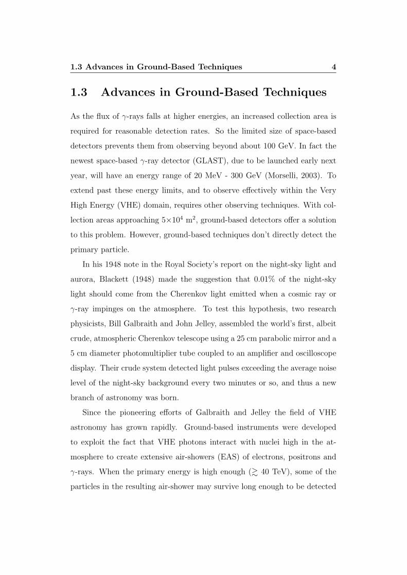
1.3 Advances in Ground-Based Techniques

As the flux of γ-rays falls at higher energies, an increased collection area is

required for reasonable detection rates. So the limited size of space-based

detectors prevents them from observing beyond about 100 GeV. In fact the

newest space-based γ-ray detector (GLAST), due to be launched early next

year, will have an energy range of 20 MeV - 300 GeV (Morselli, 2003). To

extend past these energy limits, and to observe effectively within the Very

High Energy (VHE) domain, requires other observing techniques. With col-

lection areas approaching 5×104 m2, ground-based detectors offer a solution

to this problem. However, ground-based techniques don’t directly detect the

primary particle.

In his 1948 note in the Royal Society’s report on the night-sky light and

aurora, Blackett (1948) made the suggestion that 0.01% of the night-sky

light should come from the Cherenkov light emitted when a cosmic ray or

γ-ray impinges on the atmosphere. To test this hypothesis, two research

physicists, Bill Galbraith and John Jelley, assembled the world’s first, albeit

crude, atmospheric Cherenkov telescope using a 25 cm parabolic mirror and a

5 cm diameter photomultiplier tube coupled to an amplifier and oscilloscope

display. Their crude system detected light pulses exceeding the average noise

level of the night-sky background every two minutes or so, and thus a new

branch of astronomy was born.

Since the pioneering efforts of Galbraith and Jelley the field of VHE

astronomy has grown rapidly. Ground-based instruments were developed

to exploit the fact that VHE photons interact with nuclei high in the at-

mosphere to create extensive air-showers (EAS) of electrons, positrons and

γ-rays. When the primary energy is high enough (& 40 TeV), some of the

particles in the resulting air-shower may survive long enough to be detected

1.4 Modern Satellite γ-ray Astronomy 5

at mountain level. In this case, arrays of particle detectors spread out over

a large area at high-altitude sites, can detect the secondary particles of the

EAS. With detectors located at very high altitudes it is possible to detect

secondary particles from primaries with energies & 4 - 5 TeV. At lower en-

ergies (100 GeV - 10 TeV) Cherenkov light emitted from the EAS in the

atmosphere can be detected at ground level by an optical reflector, resem-

bling the dish of a radio telescope, and a light detector consisting of an array

of photomultiplier tubes that optically image the Cherenkov photons. This is

known as the Imaging Atmospheric Cherenkov Technique and was proposed

by Weekes & Turver (1977) and pioneered at the Fred Lawrence Whipple

Observatory in southern Arizona. A full description of this technique and

the various ground-based experiments is given later in this thesis. In 1989

the first statistically significant detection of a VHE source was reported. The

Crab Nebula was detected at a 9σ confidence level using the Whipple 10 m

imaging atmospheric Cherenkov telescope (Weekes et al., 1989).

1.4 Modern Satellite γ-ray Astronomy

1.4.1 The Compton Gamma Ray Observatory

The field of space-based detection of HE photons progressed further with the

operation of NASA’s Compton Gamma Ray Observatory (CGRO) between

1991-2000. CGRO consisted of four separate instruments and covered the

energy range 30 keV to 30 GeV: OSSE (60 keV - 10 MeV), COMPTEL (800

keV - 30 MeV), BATSE (30 keV - 1.9 MeV) and EGRET (20 MeV to 30 GeV).

The Energetic Gamma Ray Experiment Telescope (EGRET) on board was

the largest γ-ray space-based detector operated to date. During its lifetime

EGRET had a huge impact on the field of high-energy astronomy, providing

1.4 Modern Satellite γ-ray Astronomy 6

numerous new sources for target observation lists for VHE astronomy.

EGRET

EGRET was of most interest to the VHE γ-ray community and during its

lifetime EGRET detected more than 70 Active Galactic Nuclei (AGN) and

seven pulsars (Mukherjee et al., 1997; Hartman et al., 1999). EGRET also

detected six Gamma Ray Bursts (GRBs) in the HE band. In addition to

these, the EGRET experiment also detected approximately 170 HE sources

not associated with any object known at other energies. Figure 1.1 illustrates

the catalogue of sources detected by the EGRET instrument. Many of these

unidentified objects populate the galactic equator and hence may be galactic

in nature. A detailed description of the EGRET instrument can be found in

Kanbach et al. (1988).

1.4.2 Next Generation Satellite Experiments

INTEGRAL

The INTEGRAL detector was launched in 2002 (Winkler et al., 2003) and

consists of four instruments: a γ-ray spectrometer (20 keV - 8 MeV), an

imager (15 keV - 10 MeV), an X-ray monitor (3 - 35 keV) and an optical

monitor. The combination of these four instruments means that INTEGRAL

can observe sources simultaneously in optical, X-ray and γ-ray bands, with

high spectral and spatial resolution, making it perfectly suited to observe

Gamma Ray Bursts (GRBs) over multiple wavelengths.

1.4 Modern Satellite γ-ray Astronomy 7

+180 −180

+90

−90

Unidentified AGN Low Conf. AGNLMC Pulsar Solar Flare

Figure 1.1: Catalogue of sources detected by EGRET during its lifetimeincluding unidentified sources, pulsars, AGN and low confidenceidentifications with AGN. Figure from Fegan (2003).

Swift

Swift was launched into a low-Earth orbit on November 20, 2004. The main

objective of its mission is the rapid response to GRB detections, recording

and reporting their locations and determining if there is also an afterglow

signal in the X-ray, ultraviolet (UV) and optical bands (Barthelmy et al.,

2001). Swift has three main co-aligned instruments onboard, the Burst Alert

Telescope (BAT), an X-ray telescope (XRT), and an UV/Optical telescope

(UVOT). BAT is a coded-aperture γ-ray imager with a wide field-of-view

that can produce arcminute GRB positions onboard within 10 seconds. The

spacecraft can execute rapid autonomous slews that point the X-ray and UV

telescopes at the BAT position in typically ∼ 50 s to provide critical afterglow

data.

1.4 Modern Satellite γ-ray Astronomy 8

GLAST

The Gamma-ray Large Area Space Telescope (GLAST), shown in Figure

1.2 (Mattox et al., 1996; Morselli, 2003) is scheduled to be launched in

2008. GLAST is the natural successor to EGRET as its instruments are

based on the same basic principles of operation. However, GLAST employs

new technologies in the hope of improving the performance of the detector.

GLAST will operate two instruments, the Large Area Telescope (LAT) and

the GLAST Burst Monitor (GBM). The LAT is an imaging γ-ray detector

sensitive to photons in the energy range 20 MeV to 300 GeV while the GBM

is designed to detect bursts of photons with energy from 5 keV to 25 MeV.

Figure 1.2: The Gamma-ray Large Area Space Telescope (GLAST). Thetop section of the spacecraft contains the LAT instrument andthe lower section contains the GBM. See text for more details.Figure from NASA (education and public outreach).

The LAT instrument is composed of alternate sheets of high-Z absorber

interlaced with silicon strip detectors for tracking motion of electron-positron

pairs. This aids in determining arrival direction of the incoming photon.

The silicon strip detectors are inexpensive, lightweight, and can offer a long

lifetime, since no consumable materials are used in their operation (such as

gas, which would be consumed in a spark chamber). An upper strip detector

1.5 Thesis Overview 9

acts as a charged-particle anti-coincidence shield, and energy measurements

are provided by a segmented CsI calorimeter located beneath the layered

strip detector. Table 1.1 summarises the various space-based detectors used

to collect data from High Energy astrophysical sources.

AGILE

AGILE is a 350 kg satellite dedicated to high-energy astrophysics funded and

managed by the Italian Space Agency (ASI) (Mereghetti et al., 2000). Its

main goal is the simultaneous detection of X-ray and γ-ray radiation in the

energy bands 15-60 keV and 30 MeV - 50 GeV with optimal imaging and

timing. AGILE was successfully launched on April 23, 2007 and is currently

in its science performance verification phase.

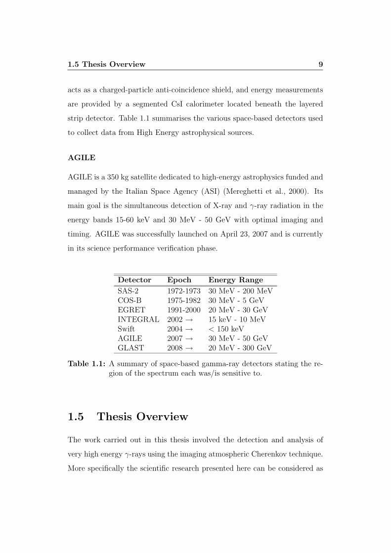
Detector Epoch Energy Range

SAS-2 1972-1973 30 MeV - 200 MeVCOS-B 1975-1982 30 MeV - 5 GeVEGRET 1991-2000 20 MeV - 30 GeVINTEGRAL 2002 → 15 keV - 10 MeVSwift 2004 → < 150 keVAGILE 2007 → 30 MeV - 50 GeVGLAST 2008 → 20 MeV - 300 GeV

Table 1.1: A summary of space-based gamma-ray detectors stating the re-gion of the spectrum each was/is sensitive to.

1.5 Thesis Overview

The work carried out in this thesis involved the detection and analysis of

very high energy γ-rays using the imaging atmospheric Cherenkov technique.

More specifically the scientific research presented here can be considered as

1.5 Thesis Overview 10

two separate sections. The first part describes work carried out on improv-

ing the optical performance of the 10 - 12 m class of imaging atmospheric

Cherenkov telescope using an innovative mirror alignment system and the

iterative deconvolution of Cherenkov images. The second part is the descrip-

tion of an in-depth reanalysis of archival data from the unidentified source

TeV J2032+4130. The reanalysis of this data led to a clearer flux determi-

nation for the 1989/1990 period of activity than was previously known.

In the sequence of this report, Chapter 2 explains the main production

mechanisms of very high energy γ-rays. Chapter 2 also describes the imag-

ing atmospheric Cherenkov technique. Chapter 3 details the specifics of

detecting γ-rays using the Whipple 10 m telescope. Chapter 4 details the

astrophysics of γ-ray emission from several relevant types of astrophysical

object and describes the main ground-based experiments that are used to

detect the electromagnetic air shower induced by very high energy photons.

Chapter 5 discusses the operational and design details of the mirror align-

ment system developed for use on the telescopes of the VERITAS array and

presents results of recent point spread function measurements carried out by

the collaboration.

The remaining work, described in Chapters 6, 7 and 8, was carried out

solely by the author. The attempted iterative deconvolution of Cherenkov

images is presented in Chapter 6 and details the work involved in developing

the Richardson-Lucy algorithm to iteratively deconvolve Cherenkov images

and presents the results of applying such image processing to Cherenkov im-

ages. Chapter 7 discusses the reanalysis of archival data from the unidenti-

fied source TeV J2032+4130 in which several analysis methods were applied

in an attempt to improve the detected signal in the data set. Following

from this, the differential and integral γ-ray fluxes were determined and pre-

1.6 Contributory Summary 11

sented. The final chapter discusses the results of the flux determination of

TeV J2032+4130. Chapter 8 also includes a discussion on possible γ-ray

production methods in light of the γ-ray flux results and recent results from

X-ray and radio observations. Due to the rapidly expanding catalogue of

VHE γ-ray sources in the field of ground-based γ-ray astronomy, informa-

tion regarding various sources and experiments can be considered current up

to the 25th of September 2007.

1.6 Contributory Summary

The work described in this thesis was carried out as part of a large interna-

tional collaborative project. The main contributions made by the author to

the collaboration are detailed here. The construction of the VERITAS align-

ment instrument (as described in Chapter 4) was carried out during the first

half of 2003 at NUI, Galway. Subsequent to its construction, the alignment

system was then shipped to southern Arizona in June of 2003 to the location

of the VERITAS array and tested on site.

Throughout the course of the project, several trips to the Fred Lawrence

Whipple Observatory in southern Arizona were made for the purposes of

astrophysical observations with the Whipple 10 m imaging Cherenkov tele-

scope. During these trips, valuable hands-on experience was obtained with

regard to the observational techniques being used. In addition to learning

about the observational techniques employed in ground based γ-ray astron-

omy, there were other areas where experience was gained. These included

point spread function measurements, mirror alignment surveys, mirror align-

ment as well as having to attend to unforseen electronic, mechanical and

tracking problems that arose during the course of observation runs. During

1.6 Contributory Summary 12

a visit to the VERITAS site, a contribution was made to the construction of

the first telescope (T1) of the VERITAS array. This contribution involved

the assembly and mounting of the individual mirror mounts of T1.

On the basis of the above contributions to the VERITAS and Whipple

programmes during the course of this Ph.D project, the author is listed as

lead author on a 29th International Cosmic Ray Conference presentation pa-

per, a co-author on 13 VERITAS Collaboration scientific publications and

co-author on the VERITAS Collaboration presentation papers of 28th and

29th International Cosmic Ray Conferences. The topics of these papers var-

ied from technical descriptions of the Whipple 10 m telescope and the VER-

ITAS array, mirror alignments of the VERITAS array, progress reports on

the VERITAS array to results from observational studies of various galactic

and extragalactic objects of interest. These observations included multi-

wavelength studies of Mrk 421, spectral studies of 1ES 1959+650, a survey

of EGRET unidentified sources using the Whipple 10 m telescope, a search

for emission from radio quasars, and observations of M87, Starburst Galax-

ies, H1426+428, TeV J2032+4130, 1ES 2344+514 and a search for primordial

black holes amongst others. A detailed list of all associated publications is

given in Appendix A.

Chapter 2

Ground-Based

γ-ray Astronomy & the

Imaging Atmospheric

Cherenkov Technique

2.1 Introduction

Following the first tentative detections of high energy photons in the 1960s

(Clark et al., 1968; Kraushaar et al., 1965), γ-ray astronomy was slow to gain

acceptance in the wider astronomical community. However, in the last fifteen

years, ground-based techniques of detecting Very High Energy (VHE) pho-

tons have evolved to the point where ground-based γ-ray astronomy is now

developing rapidly as bigger and better Cherenkov telescopes come online.

Because of these new array systems the VHE universe is rapidly becoming a

more charted region.

Modern experiments like VERITAS and HESS take new strides into this

2.2 The High Energy Universe 14

area of astronomy. In particular, results from the HESS Collaboration are

breaking new ground in making detections of astrophysical objects that ap-

pear to shine only in γ-rays as well as new detections of more traditional VHE

γ-ray sources like supernova remnants and active galactic nuclei. As such,

the catalogue of very high energy sources is rapidly expanding. This chapter

will cover the different astrophysical processes that lead to γ-ray emission

and will describe the different types of sources and possible production mod-

els that were studied during the course of this project. Descriptions of the

main ground-based γ-ray experiments that are of relevance to this work are

also given.

2.2 The High Energy Universe

Our universe is an area of contrasting activity. There are vast regions of

absolute inactivity and then there are isolated regions of unimaginable vio-

lence that lead to the emission of immense amounts of energy. Evidence of

this violence comes in the form of cosmic rays whose energy per particle can

range from 107 eV to beyond 1020 eV. It is clear that these particles must

originate in the most energetic environments in the universe such as super-

novae, active galactic nuclei (AGN) and gamma-ray bursts (GRBs). These

cosmic particle accelerators provide us with great natural laboratories that

cannot be duplicated on Earth.

Since their discovery by Hess (1912), the nature and origin of cosmic

rays has been a central focus of high energy astrophysics. As mentioned in

Chapter 1, there is an inherent inability to determine the point of origin of

charged VHE cosmic rays as they arrive at the Earth. They appear from

random directions carrying little information regarding their source and ori-

2.2 The High Energy Universe 15

gin. Since photons are uncharged, they retain directional information and

hence provide us with information regarding the point of origin.

Of the electromagnetic radiation that can be detected on Earth, it is

the photons of the highest energy that are of interest to γ-ray astronomy.

It is these photons that provide us with direct evidence of the locations of

the very high energy galactic and extra-galactic processes in the Universe.

Since VHE γ-rays are neutral, they can only be produced by secondary in-

teractions involving other charged particles, for example the collision of a

hadronic beam with matter that produces secondary pions which then de-

cay into γ-rays (Mannheim, 1993; Romero et al., 2003). VHE γ-rays may

also be produced via a leptonic process, for example emission due to the Syn-

chrotron Self-Compton (SSC) model in which lower energy photons produced

via synchrotron emission from relativistic electrons that are then up-scattered

to very high energies by their parent electrons (Blumenthal & Gould, 1970;

Maraschi et al., 1992; Atoyan & Aharonian, 1999; Bosch-Ramon et al., 2006).

The presence of VHE γ-rays in regions of our galaxy and beyond, suggests

areas of particle acceleration to energies of an order of magnitude greater

than that of the γ-rays themselves.

Before experiments could provide direct detections of these VHE pho-

tons, work by Feenberg & Primakoff (1948), Hayakawa (1952), and Morrison

(1958) advocated the potential importance of γ-ray astronomy as a method

of studying high-energy astrophysical processes directly. Since these early

theoretical studies, there have been technological advances that have pro-

vided a means of detecting these VHE photons. Recent developments have

seen many advances in both ground-based and satellite-borne γ-ray detec-

tion, leading to a revolution in the field and moving it from a little understood

curiosity to a mainstream branch of astronomy.

2.2 The High Energy Universe 16

Classification Energy Range Detection Technique

Low Energy (LE) 0.1 - 10 MeV Scintillator(Satellite)

Medium Energy (ME) 10 - 30 MeV Compton Telescope(Satellite)

High Energy (HE) 30 MeV - 0.1 TeV Spark Chamber(Satellite)

Very High Energy (VHE) 0.1 TeV - 100 TeV Ground-based:Cherenkov Telescope(Mountain/Sea Level)

Ultra High Energy (UHE) 0.1 PeV - 100 PeV Ground-based:Air Shower Array

(Mountain)Extremely High Energy (EHE) > 100 PeV Ground-based:

Fluorescence detector(Sea Level)

Table 2.1: Subdivisions of the γ-ray spectrum, the labels used to differ-entiate between energy bands and the corresponding detectionmethods. Adapted from Weekes (1988)

The γ-ray energy domain is the most extensive of the electromagnetic

spectrum, spanning at least fifteen decades in energy. Weekes (2003) defines

the γ-ray as a generic term used to describe photons of energy from about

500 keV to > 100 EeV. This range is as large as the rest of the observed

spectrum combined and a variety of detector technologies is required to span

it. Therefore, it is convenient to introduce several subdivisions, taking into

account the specific scientific objectives and detection methods relevant to

different energy bands. Generally, observational γ-ray astronomy can be

divided into five bands, defined by Weekes (1988) as: Low Energy (LE),

Medium Energy (ME), High Energy (HE), Very High Energy (VHE) and

2.3 Astrophysical Production Mechanisms of TeV γ-rays. 17

Ultra High Energy (UHE). These conventional subdivisions are shown in

Table 2.1 along with their corresponding energy ranges in eV.

While low to high energy γ-rays are observed by satellite or balloon-

borne detectors, the highest energy γ-ray regimes (VHE and UHE) are best

detected using ground-based instruments. It is the VHE range which is

investigated in this thesis.

2.3 Astrophysical Production Mechanisms of

TeV γ-rays.

Electromagnetic radiation can be considered to be thermal or non-thermal in

origin. Thermal radiation, or blackbody radiation, is emitted from a hot body

such as a star. The emission spectrum is a function of the temperature of the

hot body. Total intensity of the emitted radiation is directly proportional

to the temperature of the star raised to the fourth power, i.e., I ∝ T4. For

hot stars with surface temperatures of around 104 Kelvin, the peak thermal

emission occurs at an energy less than 1 keV. Since the spectra of sources

of VHE γ-rays can have peak energies greater than 107 eV, it is clear that

γ-rays are a form of non-thermal radiation. The production of non-thermal

radiation is due to the acceleration of charged particles and, in order to

explain the origin of galactic γ-rays, an understanding of the acceleration

mechanisms involved is required. The following section outlines the principal

processes responsible for the production of γ-ray photons. These processes

can generally be divided into several groups, each of which is briefly discussed.

2.3 Astrophysical Production Mechanisms of TeV γ-rays. 18

2.3.1 Acceleration of Charged particles

There are several processes (Hillier, 1984; Aharonian, 2004) that can accel-

erate charged particles and, hence, result in the emission of electromagnetic

radiation. With regard to the astrophysical objects studied in this work,

the leading γ-ray production models specific to these sources are discussed

in detail later in this chapter. The main production mechanisms resulting

in non-thermal γ-ray emission via particle acceleration are briefly described

here.

Synchrotron Radiation

The simplest form of accelerated motion of a charged particle in a magnetic

field is due to non-relativistic gyration around the field line. Emission due to

this acceleration is known as cyclotron radiation. When observed, circularly

polarised or linearly polarised waves are detected radiating from the charged

particle. The polarisation depends on the orientation of the observer relative

to the magnetic field direction.

Cyclotron radiation will change to synchrotron radiation when the speed

of the charged particle moving in the magnetic field approaches the speed of

light. To achieve production of synchrotron radiation at γ-ray energies, ultra-

relativistic electrons must be moving in extremely strong magnetic fields, see

Figure 2.1. If the electron is traveling relativistically with a Lorentz factor γ,

the emission is beamed tangentially in a narrow cone of half angle ∼ 1/γ di-

rected along the instantaneous direction of motion.1 A continuous spectrum

of polarised radiation results since there is a large population of relativistic

electrons each emitting at different frequencies. The overall spectrum of the

1The Lorentz factor γ = 1√1−β2

where β = u/c with the particle velocity u and speed

of light c.

2.3 Astrophysical Production Mechanisms of TeV γ-rays. 19

Figure 2.1: A representation of synchrotron radiation production. As theelectron spirals along a magnetic field line, a cone of syn-chrotron radiation is emitted at a tangent to the electron’strajectory.

emission consists of the sum of a large number of harmonics of the basic

cyclotron emission. The spectrum has a peak, with maximum emission at

νc, where νc is the critical frequency:

νc =γ2eB

2πme

3

2sinθ (2.1)

where B is the magnetic field strength perpendicular to the direction of

motion and θ is the pitch angle between the particle trajectory and the

direction of the magnetic field. While emitting synchrotron radiation an

electron will cool as its energy is depleted. The rate of this cooling is given

by:

dEe

dt= 10−14B2γ2 (2.2)

2.3 Astrophysical Production Mechanisms of TeV γ-rays. 20

The electron will lose half its energy by synchrotron emission in a time t

given by:

t =5

γB2(2.3)

An electron population radiating in an astrophysical environment will

typically have a power-law spectrum:

dNe

dEe

∝ E−pe (2.4)

and the resulting synchrotron radiation will have a spectral energy distribu-

tion Fν ∝ να where

α =1− p

2(2.5)

The study of the synchrotron spectrum can provide much insight into

the particle population within a cosmic accelerator. It can be noted that

higher-energy electrons radiate more rapidly and thus lose energy faster. The

depletion of the higher energy electrons would lead to a steeper power-law

synchrotron spectrum above the critical frequency (νc) which is dependent

on the magnetic field

A source emitting high-energy radiation with a power-law spectrum and

with a high degree of polarisation would generally indicate that synchrotron

acceleration is present. To produce γ-rays directly by synchrotron radiation,

either the electrons must be very highly relativistic, or a very intense mag-

netic field is required. The observation of a synchrotron component can also

indicate the presence of relativistic electrons which may provide a target field

for photons and generate γ-rays by the inverse-Compton mechanism.

2.3 Astrophysical Production Mechanisms of TeV γ-rays. 21

Figure 2.2: Frequency distribution of synchrotron electrons showing thecharacteristic peak emission near 0.29νc where νc is the crit-ical frequency as defined in Equation 2.1

Inverse-Compton Scattering

When a high energy electron collides with a lower energy photon there is

a transfer of energy from the electron to the photon (Figure 2.3). This in-

teraction is of considerable importance in astrophysical environments where

the density of low-energy photons is high and where there is a supply of

relativistic electrons. The process known as the synchrotron self-Compton

process occurs when low energy synchrotron photons gain energy from the

same population of electrons from which they originate. The synchrotron

self-Compton production mechanism is assumed to be the main VHE γ-

ray production mechanism that results in VHE emission from supernova

remnants (Cowsik & Sarkar, 1980; Allen et al., 1997) and possibly active

galactic nuclei (Krawczynski et al., 2002; Wilson, 2001). Calculated syn-

chrotron self-Compton spectra provide a good fit to the observed spectrum

from the Crab Nebula (de Jager et al., 1996).

2.3 Astrophysical Production Mechanisms of TeV γ-rays. 22

SynchrotronX−ray

TeV γ

Synchrotron e−

Figure 2.3: A representation of Inverse-Compton Scattering.

In the collision between a relativistic electron with energy Ee = γmec2

and a photon of energy ε = hν, the scattered photon energy in the laboratory

system, averaged over all angles of incidence and scattering, is ≈ 43γ2ε. This

process can turn a radio photon into a γ-ray photon. The low-energy photons

may belong to the cosmic background radiation (T = 2.7 K), which has an

energy density of 0.4× 10−13 J.m−3. Alternatively, as mentioned above, the

low-energy photons may be the synchrotron photons emitted by the energetic

electron population itself.

The energy transferred to the photon depends on the cross-section and on

the scattering angle at which the electron and photon meet. For a maximum

energy transfer (Emax), the particles must meet head-on, reversing the photon

direction in the collision, while a minimum energy (Emin) will be transferred

when the scattering angle is 90.

The probability of the electron-photon interaction, i.e. the cross-section,

is given by the Klein-Nishina formula:

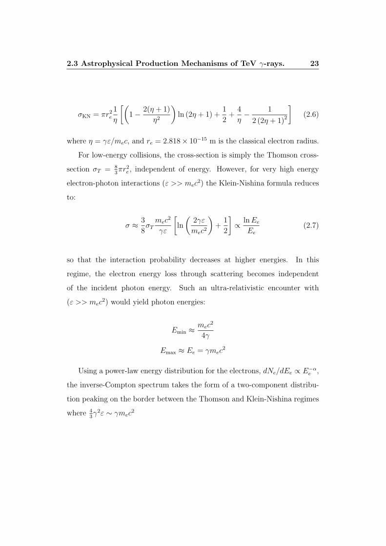
2.3 Astrophysical Production Mechanisms of TeV γ-rays. 23

σKN = πr2e

1

η

[(1− 2(η + 1)

η2

)ln (2η + 1) +

1

2+

4

η− 1

2 (2η + 1)2

](2.6)

where η = γε/mec, and re = 2.818× 10−15 m is the classical electron radius.

For low-energy collisions, the cross-section is simply the Thomson cross-

section σT = 83πr2

e , independent of energy. However, for very high energy

electron-photon interactions (ε >> mec2) the Klein-Nishina formula reduces

to:

σ ≈ 3

8σT

mec2

γε

[ln

(2γε

mec2

)+

1

2

]∝ ln Ee

Ee

(2.7)

so that the interaction probability decreases at higher energies. In this

regime, the electron energy loss through scattering becomes independent

of the incident photon energy. Such an ultra-relativistic encounter with

(ε >> mec2) would yield photon energies:

Emin ≈ mec2

4γ

Emax ≈ Ee = γmec2

Using a power-law energy distribution for the electrons, dNe/dEe ∝ E−αe ,

the inverse-Compton spectrum takes the form of a two-component distribu-

tion peaking on the border between the Thomson and Klein-Nishina regimes

where 43γ2ε ∼ γmec

2

2.4 The Imaging Atmospheric Cherenkov Technique 24

2.3.2 Particle Decay

When a particle decays, a γ-ray may be produced. An example of such a

process is the decay of a neutral pion.

π0 → 2γ

Pions are created during strong interaction events. These events could be

the collisions of cosmic rays with the nuclei of interstellar gas clouds. For

example a common interaction of a cosmic ray proton is a collision with

stationary hydrogen gas, producing excited states that lead to the emission

of π mesons. The most common interaction has the form:

p + p → N + N + π+ + π− + π0

where N is a proton or neutron. The neutral pion (π0) is unstable and decays

rapidly (with a half-life ∼ 10−16 s) into two photons. The energy distribution

peaks at half the rest mass of the pion∼ 70 MeV. This peak is the characteris-

tic feature of p-p interactions and the signature of hadrons as the progenitors

in γ-ray sources. Pions that decay while traveling at relativistic velocities

may produce VHE or UHE γ-rays. The decay of subatomic particles is also

an important factor in the development of electromagnetic cascades in the

atmosphere. There is also the possibility that VHE γ-rays may be created

by the annihilation of dark matter.

2.4 The Imaging Atmospheric Cherenkov Tech-

nique

The key element to the success of ground-based γ-ray astronomy in detecting

very high energy (VHE) photons in the 50GeV to 50TeV range lies with the

2.4 The Imaging Atmospheric Cherenkov Technique 25

imaging atmospheric Cherenkov technique. This chapter will describe the

imaging atmospheric Cherenkov technique, its associated instruments, and

analysis methods, as pioneered by the Whipple collaboration.

An atmospheric Cherenkov telescope is very different to an optical tele-

scope, and superficially it has the appearance of a radio telescope. Since the

atmosphere is opaque to high-energy photons, the atmospheric Cherenkov

telescope doesn’t physically detect the γ-ray photon but instead detects its

interactions with nuclei high up in the earth’s atmosphere. These interactions

lead to showers of secondary particles that can be detected at ground level

by means of the imaging atmospheric Cherenkov technique and telescope.

The result of the shower of secondary particles in the atmosphere is a

brief, faint flash of Cherenkov light emitted in the ultraviolet/visible range.

The atmospheric Cherenkov telescope then detects this faint light and recon-

structs the energy and direction of the original VHE photon that produced

the air shower. Unlike space-based γ-ray detectors whose collection areas

can be restrictive in size, the imaging atmospheric Cherenkov technique uses

the Earth’s atmosphere as its detector. An atmospheric Cherenkov telescope

with a physical aperture of ∼ 10 m can have an effective collection area of ∼5 x 104 m2.

The first statistically significant detection of VHE γ-ray emission was re-

ported by the Whipple Collaboration in 1989 using the imaging atmospheric

Cherenkov technique (Weekes et al., 1989). The source under study at the

time was the much observed Crab Nebula supernova remnant (Figure 2.4).

2.5 Cherenkov Radiation 26

Figure 2.4: The Crab Nebula supernova remnant observed with the HubbleSpace Telescope. Figure courtesy of the Hubble Heritage Team(heritage.stsci.edu).

2.5 Cherenkov Radiation

2.5.1 Introduction

Cherenkov radiation is electromagnetic radiation emitted when a charged

particle passes through a transparent medium at a speed greater than the

speed of light in that medium. It is named after the Russian scientist Pavel

Alekseyevich Cherenkov who won the 1958 Nobel Prize after his intensive

studies of this phenomenon (Cherenkov et al., 1958). The speed of light

in a vacuum is a universal constant (c), however the speed of light in a

material can be significantly less than c. When cosmic rays, traveling close

to c enter the Earth’s atmosphere (the medium) at a speed greater than the

phase velocity of light in that medium, the result is a very brief flash of light.

2.5 Cherenkov Radiation 27

A common analogy to use here is that of the sonic boom of a supersonic

aircraft. The sound waves created by the aircraft do not move fast enough to

get out of the way of the aircraft. This results in the waves stacking up and

a shock front is formed. Similarly, superluminal charged particles generate

photonic shock waves as they travel through the Earth’s atmosphere that

manifest themselves as a very brief flash of light towards the blue end of the

spectrum. For a detailed description on the characteristics and production of

Cherenkov radiation see Jelley & Porter (1963). The following gives a brief

outline of the production of Cherenkov radiation.

2.5.2 Cherenkov radiation production

When a charged particle passes through a dielectric medium, it polarises the

atoms close to where it passes. Once it has passed, the atoms can then relax

back to their initial state and in doing so emit a brief pulse of electromagnetic

radiation. When these pulses are emitted coherently, Cherenkov radiation

Figure 2.5: Left: Cherenkov radiation wavefront production. Right: Thecone shape trajectory of the charged particle. Note theCherenkov angle is the apex angle.

results. For the pulses to be in phase, the particle must travel through the

2.5 Cherenkov Radiation 28

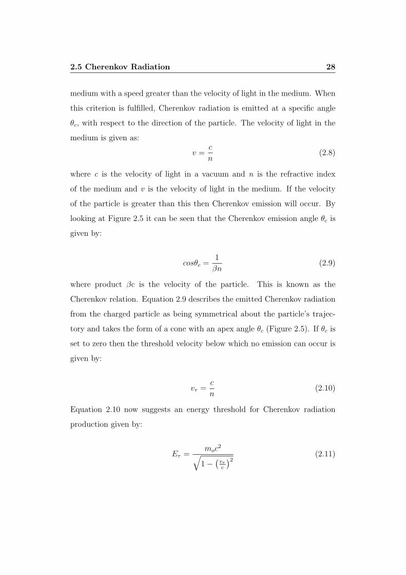
medium with a speed greater than the velocity of light in the medium. When

this criterion is fulfilled, Cherenkov radiation is emitted at a specific angle

θc, with respect to the direction of the particle. The velocity of light in the

medium is given as:

v =c

n(2.8)

where c is the velocity of light in a vacuum and n is the refractive index

of the medium and v is the velocity of light in the medium. If the velocity

of the particle is greater than this then Cherenkov emission will occur. By

looking at Figure 2.5 it can be seen that the Cherenkov emission angle θc is

given by:

cosθc =1

βn(2.9)

where product βc is the velocity of the particle. This is known as the

Cherenkov relation. Equation 2.9 describes the emitted Cherenkov radiation

from the charged particle as being symmetrical about the particle’s trajec-

tory and takes the form of a cone with an apex angle θc (Figure 2.5). If θc is

set to zero then the threshold velocity below which no emission can occur is

given by:

vτ =c

n(2.10)

Equation 2.10 now suggests an energy threshold for Cherenkov radiation

production given by:

Eτ =moc

2

√1− (

vτ

c

)2(2.11)

2.6 Extensive Air Showers 29

For an electron moving through the atmosphere (refractive index 1.00029 at

sea level) the energy threshold is ∼ 21 MeV. When the particle moves with a

velocity of vp/c → 1, (at very high relativistic velocities) the maximum angle

of Cherenkov emission is given by:

θmax = cos−1

(1

n

)(2.12)

The Cherenkov angle is 1.3° at sea level and decreases with altitude. The

energy thresholds for Cherenkov radiation production for muons and protons

are 4.4 GeV and 39 GeV respectively. Since there are higher populations

of electrons in an extensive air showers, it is generally expected that they

contribute to the majority of Cherenkov light in extensive air showers.

2.6 Extensive Air Showers

When a VHE photon or cosmic ray impinges on the top of the atmosphere, a

cascade of secondary particles is initiated. Providing the energy of secondary

particles in the shower is greater than Eτ from Equation 2.11, Cherenkov

light will be generated. The resulting shower can contain ∼ 105 secondary

particles. At ground level these showers can cover an area of approximately

105 m2 and are known as Extensive Air Showers (EAS).

2.6.1 Electromagnetic Air Showers

γ-ray initiated EAS are produced when a VHE photon interacts or passes

close to the nucleus of an atom in the atmosphere and produces a relativistic

electron/positron pair:

γ → e+e−

2.6 Extensive Air Showers 30

For the ultra-relativistic case of an air shower, the radiation length2 for pair-

production is 37.7 g cm−2. This means that a γ-ray induced shower is ini-

tiated near the top of the atmosphere (total depth of the atmosphere is ∼1000 g cm−2). Figure 2.6 shows the processes involved in a γ-ray induced

EAS.

Figure 2.6: Gamma-ray shower development.

The first pair-produced secondary electrons (electron/positron) only travel

a short distance before interacting with other nuclei to produce two new

high-energy γ-rays. This process repeats, producing more secondary elec-

trons and γ-rays. The shower will grow exponentially until ionisation losses

are approximately equal to radiation losses. At this point, for a 100 GeV

2The mean distance a particle will travel before interacting with another particle.

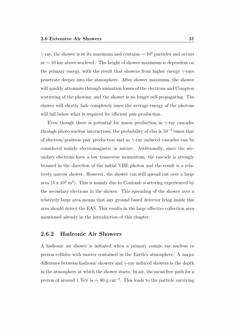
2.6 Extensive Air Showers 31

γ-ray, the shower is at its maximum and contains ∼ 102 particles and occurs

at ∼ 10 km above sea level . The height of shower maximum is dependent on

the primary energy, with the result that showers from higher energy γ-rays

penetrate deeper into the atmosphere. After shower maximum, the shower

will quickly attenuate through ionisation losses of the electrons and Compton

scattering of the photons, and the shower is no longer self-propagating. The

shower will shortly fade completely since the average energy of the photons

will fall below what is required for efficient pair production.

Even though there is potential for muon production in γ-ray cascades

through photo-nuclear interactions, the probability of this is 10−4 times that

of electron/positron pair production and so γ-ray induced cascades can be

considered mainly electromagnetic in nature. Additionally, since the sec-

ondary electrons have a low transverse momentum, the cascade is strongly

beamed in the direction of the initial VHE photon and the result is a rela-

tively narrow shower. However, the shower can still spread out over a large

area (3 x 104 m2). This is mainly due to Coulomb scattering experienced by

the secondary electrons in the shower. This spreading of the shower over a

relatively large area means that any ground based detector lying inside this

area should detect the EAS. This results in the large effective collection area

mentioned already in the introduction of this chapter.

2.6.2 Hadronic Air Showers

A hadronic air shower is initiated when a primary cosmic ray nucleus or

proton collides with matter contained in the Earth’s atmosphere. A major

difference between hadronic showers and γ-ray induced showers is the depth

in the atmosphere at which the shower starts. In air, the mean free path for a

proton of around 1 TeV is ∼ 80 g cm−2. This leads to the particle surviving

2.6 Extensive Air Showers 32

to a greater atmospheric depth a than for a γ-ray which has a mean free

path of 37 g cm−2. The implication is that for a γ-ray induced shower and

a hadron induced shower of the same energy, there is normally a greater

number of particles reaching detector level from the hadronic shower. The

collisions between the cosmic ray and atmospheric matter cause the primary

hadron to lose much of its initial energy by producing nucleons and pions

and other secondary particles, all of which are beamed in the direction of

the primary particle. The neutral pions decay into photons and the charged

pions decay into muons via the following decay mechanisms:

π0 → 2γ

π+ → µ+ + νµ

π− → µ− + νµ

The muons are weakly interacting and do not contribute any further to

the shower development, but can themselves initiate smaller electromagnetic

cascades that do contribute. However, since relativistic muons have relatively

long lifetimes, they can sometimes remain in the shower until they reach

ground level. If the trajectory of a local muon is parallel to the optic axis

then, depending on its distance from the optic axis, local muons can produce

Cherenkov images similar to showers initiated by low energy (< 200 GeV)

γ-rays. The image generated by the local muon in the camera may appear

as a full ring or, a partial ring. This can have a detrimental effect when

trying to distinguish between γ-ray induced showers and hadronic showers,

especially with single ground-based detectors.

Other secondary nucleons and charged pions will continue to multiply

in successive generations until each particle’s energy drops below ∼ 1 GeV

(energy required for multiple pion production). The γ-rays produced by

2.6 Extensive Air Showers 33

the decay of the π0 pair produce to create smaller electromagnetic cascades,

which are self regenerating and so are the dominating element in hadronic air

showers. Once the shower maximum is reached, the electrons and positrons

will lose most of their energy through ionisation losses. Figure 2.7 illustrates

a simplistic graphical representation of a hadronic shower cascade.

Figure 2.7: Hadronic shower development.

A major difference between hadronic showers and γ-ray showers is that

the hadronic showers tend to be less compact and more random in shape

and orientation than γ-ray showers. This is due to larger fluctuations and

large opening angles of the pion interactions resulting in larger transverse

momentum being given to particles during the shower development. This

is an important consideration in that it gives ground-based detectors the

2.7 Discrimination between hadronic and γ-ray initiated EAS 34

potential for discrimination between hadronic showers and γ-ray showers.

2.7 Discrimination between hadronic and γ-

ray initiated EAS

To discriminate between cosmic rays and γ-rays, an atmospheric Cherenkov

telescope must have a dedicated data acquisition system to record and iden-

tify the EAS it detects. The main task of discrimination between the two

types of showers is carried out off-line after the observations have been com-

pleted.

As discussed previously, the nature of the primary particle in an air shower

governs the air shower’s development through the atmosphere, resulting in

several differences between hadronic showers and γ-ray showers. It is these

subtle differences that are exploited when discriminating between showers

initiated by hadrons and showers initiated by γ-rays. For instance, a γ-ray

is undeflected by galactic and inter-stellar magnetic fields and travels in a

straight line from its origin. In other words, the γ-ray initiated shower will be

aligned in the direction of the source. This is an advantage when compared

with cosmic rays, whose arrival directions have been altered by galactic and

interstellar magnetic fields and appear isotropically across the sky.

Early computer simulations were performed by Hillas (1985) to investi-

gate the differences between γ-ray and cosmic ray initiated EAS. The re-

sults of these simulations suggested that discrimination should be possible

by analysing the Cherenkov images on the basis of their shape and orienta-

tion as they appear on the Cherenkov imaging detector. Further descriptions

of simulations of the EAS induced by cosmic rays and γ-rays can be found

in Kertzman & Sembroski (1994) and Mohanty (1995). This section will

2.7 Discrimination between hadronic and γ-ray initiated EAS 35

γin −ray showers

1 TeV −rayγ

Mt. Hopkins

Sea Level0100m 100m

Main emissionregion of light

Main emissionregion of light

for a proton shower

1 TeV proton

km

6

5

13

12

11

4

3

1

10

9

8

2

7

21m

70m

8.1 km

Figure 2.8: A simple model of Cherenkov radiation produced by γ-raysand hadrons. The diagram illustrates some of the differencesbetween hadron-induced showers and γ-ray induced showers.The shaded region represents the maximum extent of a γ-rayinduced shower while the dashed box the maximum extent ofa hadron-induced shower. Also shown is the altitude whereshower maximum occurs (Hillas, 1996).

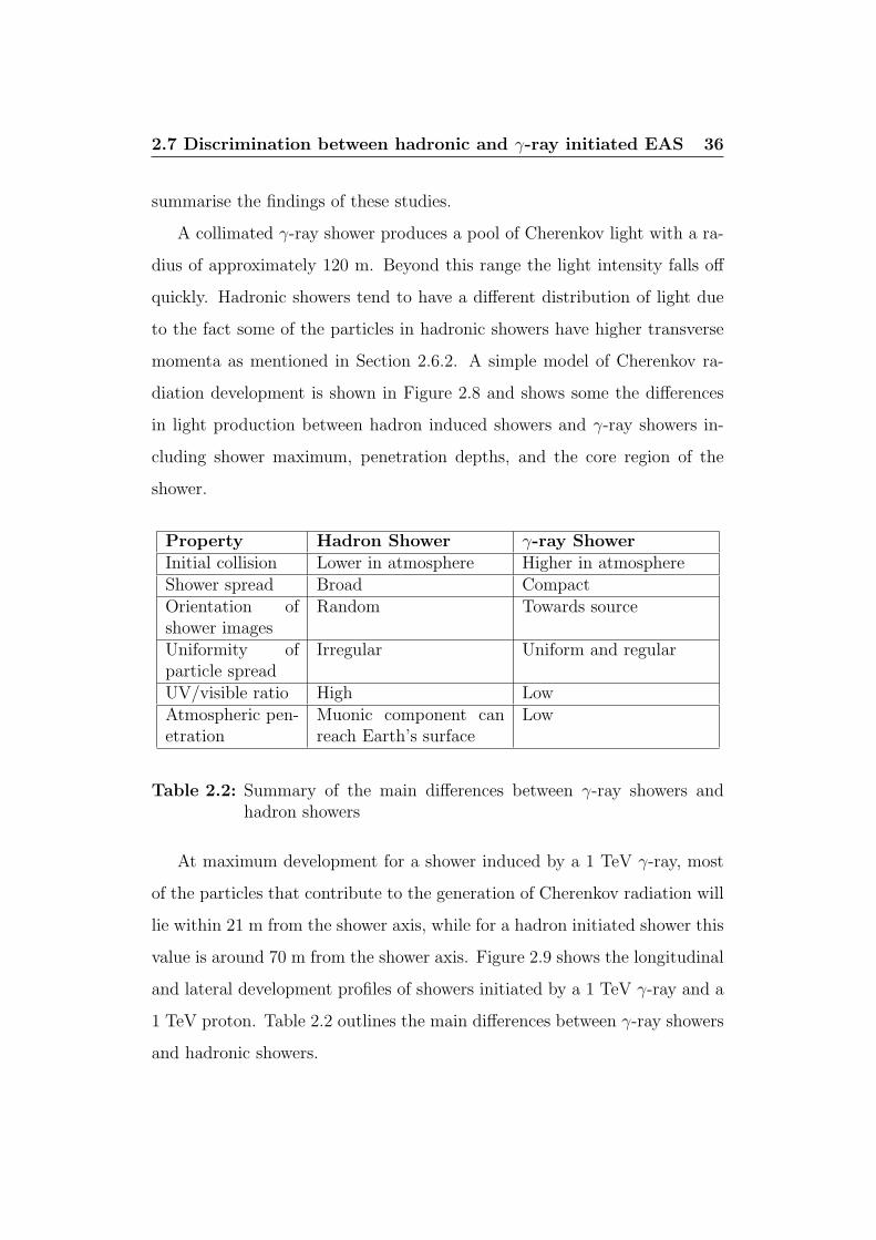
2.7 Discrimination between hadronic and γ-ray initiated EAS 36

summarise the findings of these studies.

A collimated γ-ray shower produces a pool of Cherenkov light with a ra-

dius of approximately 120 m. Beyond this range the light intensity falls off

quickly. Hadronic showers tend to have a different distribution of light due

to the fact some of the particles in hadronic showers have higher transverse

momenta as mentioned in Section 2.6.2. A simple model of Cherenkov ra-

diation development is shown in Figure 2.8 and shows some the differences

in light production between hadron induced showers and γ-ray showers in-

cluding shower maximum, penetration depths, and the core region of the

shower.

Property Hadron Shower γ-ray ShowerInitial collision Lower in atmosphere Higher in atmosphereShower spread Broad CompactOrientation ofshower images

Random Towards source

Uniformity ofparticle spread

Irregular Uniform and regular

UV/visible ratio High LowAtmospheric pen-etration

Muonic component canreach Earth’s surface

Low

Table 2.2: Summary of the main differences between γ-ray showers andhadron showers

At maximum development for a shower induced by a 1 TeV γ-ray, most

of the particles that contribute to the generation of Cherenkov radiation will

lie within 21 m from the shower axis, while for a hadron initiated shower this

value is around 70 m from the shower axis. Figure 2.9 shows the longitudinal

and lateral development profiles of showers initiated by a 1 TeV γ-ray and a

1 TeV proton. Table 2.2 outlines the main differences between γ-ray showers

and hadronic showers.

2.7 Discrimination between hadronic and γ-ray initiated EAS 37

(a) γ-ray (b) Cosmic ray

2.9: An illustration of the longitudinal development of a simulated 1 TeV γ-ray initiated shower (left) and a 1 TeV proton-initiated shower (right)(Rodgers, 1997).

2.7 Discrimination between hadronic and γ-ray initiated EAS 38

2.7.1 Detecting Cherenkov Radiation

There are several methods that can be employed to detect the EAS caused

by high-energy particles impacting with nuclei in the Earth’s atmosphere.

Figure 2.10 illustrates the main detection methods used in γ-ray astronomy.

For the imaging atmospheric Cherenkov technique the basic requirements

are, a light collector, a fast detector (photo-multiplier tube (PMT) array),

a data acquisition system to record the Cherenkov flashes, and software to

analyse the images. The main task of the atmospheric Cherenkov telescope

is the need to be able to differentiate a typical Cherenkov flash from a 1 TeV

γ-ray induced shower, that lasts for ∼ 5 ns and yields about 100 photons m−2,

from the dominant night sky flux of ∼ 1012 photons m−2s−1sr−1 between 330

and 450 nm. If the field of view of the telescope is matched to the angular

extent of the Cherenkov flash (∼ 1°), then only 1 or 2 optical photons m−2

are detected from the night-sky in 5 ns. Thus, using a suitable detector with

fast integration times, the Cherenkov flash can be easily detected above the

night-sky background.

This means that the night-sky background is one of the main factors in

determining the energy threshold for an atmospheric Cherenkov telescope

system (Cawley & Weekes, 1995). For a simple detector comprising of a

single photomultiplier tube situated at the focus of a reflecting dish, and

assuming the noise is Poissonion, the signal to noise ratio is given by:

S

N=

∫ λ2

λ1C(λ)ε(λ)Adλ√∫ λ2

λ1B(λ)ε(λ)ΩtAdλ

=

∫ λ2

λ1

C(λ)

√ε(λ)A

B(λ)tΩdλ (2.13)

where

C(λ) is the Cherenkov photon flux

2.7 Discrimination between hadronic and γ-ray initiated EAS 39

Figure 2.10: Various methods of cosmic and γ-ray detection used in γ-ray astronomy (Schroedter, 2004).

2.7 Discrimination between hadronic and γ-ray initiated EAS 40

B(λ) is the background light flux

ε(λ) is the quantum efficiency of the PMT

Ω is the solid angle

t is the integration time (must be ≥ the length of the Cherenkov flash)

A is the mirror area

λ1 and λ2 specify the wavelength range over which the PMTs are re-

sponsive.

So the smallest detectable Cherenkov flash is inversely proportional to the

signal to noise ratio giving a expression for the energy threshold (E t) of the

detector as:

Et ∝ 1

C(λ)

√B(λ)tΩ

ε(λ)A(2.14)

By making the detector as large as possible, and matching the integration

time to the duration of the Cherenkov flash, the minimum-energy threshold

can be obtained. The minimum energy air shower detectable can be opti-

mised further by maximising the quantum efficiency of the PMTs used. By

having these parameters optimised, the atmospheric Cherenkov telescope will

detect Cherenkov flashes above night-sky background.

Chapter 3

The Whipple 10 m Telescope

3.1 Introduction

This chapter describes the operation of the Whipple 10 m telescope operated

and maintained by the VERITAS Collaboration in Southern Arizona. The

Figure 3.1: The Whipple 10 m γ-ray telescope.

3.1 Introduction 42

Whipple 10 m telescope (Figure 3.1) is located at the Fred Lawrence Whipple

Observatory on Mt. Hopkins in South East Arizona (longitude 110°53.1’W,

latitude 31°41.3’N, and 2320 m above sea level). The dry desert climate and

clear skies in Southern Arizona are ideal for ground-based γ-ray astronomy.

The Whipple 10 m reflector was built in 1969 (Weekes et al., 1972) and its

primary function is the search for sources of VHE γ-rays. Since its imaging

systems were installed in 1982, it has been in continual use and was the most

effective and active instrument in the field of ground-based γ-ray astronomy

during the 90s. However a series of newer instruments have recently super-

seded it in terms of sensitivity and reliability (Hofmann et al., 2000; Weekes

et al., 2002).

The telescope can be considered the sum of two components: the reflector

and the detector or camera. Although the detector has undergone many

changes and modifications in an attempt to enhance the sensitivity of the

instrument (Fegan et al., 1983; Cawley et al., 1990; Finley et al., 2001), the

reflector is much as it was when it was first constructed.

3.1.1 Davies-Cotton Reflector Design

The reflector design is based on the Quartermaster solar-collector design

as proposed by Davies & Cotton (1957) and was first used for astronomical

purposes by Hanbury-Brown (1966). In the Davies-Cotton design the optical

support structure (OSS) or dish section of a light collecting instrument is

spherical in shape and has a radius of curvature exactly half that of the

individual mirror facets that make up its tessellated structure. Cherenkov

light is collected by the reflecting dish and focused to a detector located at

the focal point of the reflector. The main advantages of the Davies-Cotton

design include the fact that all facet mirrors are identical, the structure is

3.1 Introduction 43

rigid, off-axis aberrations are reduced and the facet alignment procedure is

relatively straight forward. With regard the off-axis properties, the Davies-

Cotton design is considered superior to that of a parabolic reflector (Lewis,

1990).

The design does however have a disadvantage in that it is not isochronous.

Due to its spherical shape, parallel rays of light from a source reach the outer

mirror facets first and, as a result, reach the focal plane before rays reflected

from the inner portion of the reflector. This causes a temporal broadening

of the optical signal detected by the PMT camera on the order of ∼ 6 ns,

requiring a longer integration time. This has the effect of reducing the signal

to noise ratio. Nevertheless, this reduction is negligible in comparison to the

noise contributions of the electronics when the signal is processed later in the

data acquisition systems. A further downside of this temporal aberration is

that the temporal properties of the Cherenkov light pulse cannot be investi-

gated. Even though the an-isochronous characteristics of the Davies-Cotton

design are an undesired attribute, it does not constitute a serious constraint

to the detection of VHE γ-rays with the Whipple 10 m telescope.

The Whipple 10 m optical reflector consists of 248 identical hexagonal

mirror facets which are mounted on the optical support structure. Each

mirror facet has a radius of curvature of 14.6 m. The facets are arranged

in a hexagonal pattern of nine concentric rings, covering a spherical dish of

radius of curvature 7.3 m and an opening diameter of 10 m. The focal plane

is located at the centre of curvature of the dish, resulting in an f/0.7 system.

The mirrors can be manually aligned by placing an alignment instrument on

the optic axis at a position twice the dish radius of curvature from the tele-

scope. This is known as the alignment point. A discussion of the alignment

procedure will be given in Chapter 4. Figure 3.2 shows a ray-trace of a beam

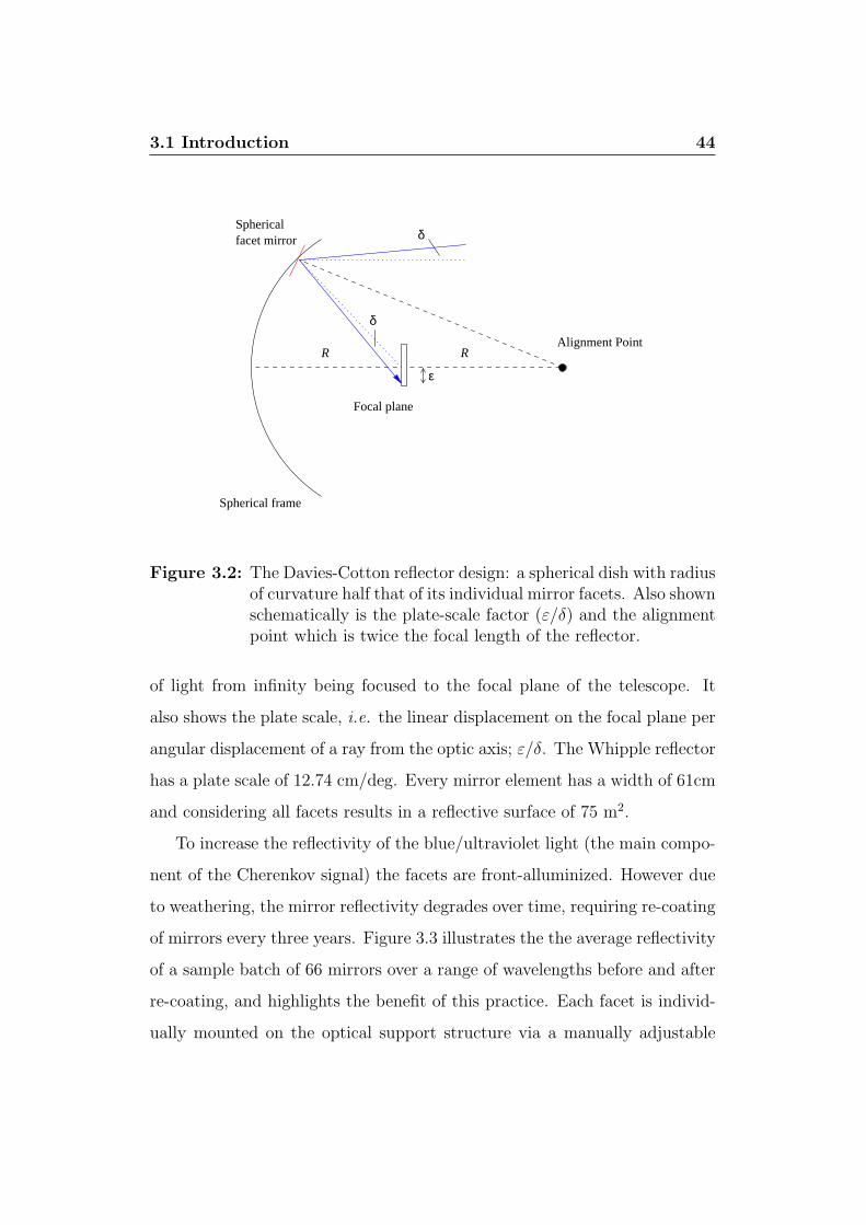
3.1 Introduction 44

Sphericalfacet mirror

Alignment PointR R

Focal plane

ε

δ

δ

Spherical frame

Figure 3.2: The Davies-Cotton reflector design: a spherical dish with radiusof curvature half that of its individual mirror facets. Also shownschematically is the plate-scale factor (ε/δ) and the alignmentpoint which is twice the focal length of the reflector.

of light from infinity being focused to the focal plane of the telescope. It

also shows the plate scale, i.e. the linear displacement on the focal plane per

angular displacement of a ray from the optic axis; ε/δ. The Whipple reflector

has a plate scale of 12.74 cm/deg. Every mirror element has a width of 61cm

and considering all facets results in a reflective surface of 75 m2.

To increase the reflectivity of the blue/ultraviolet light (the main compo-

nent of the Cherenkov signal) the facets are front-alluminized. However due

to weathering, the mirror reflectivity degrades over time, requiring re-coating

of mirrors every three years. Figure 3.3 illustrates the the average reflectivity

of a sample batch of 66 mirrors over a range of wavelengths before and after

re-coating, and highlights the benefit of this practice. Each facet is individ-

ually mounted on the optical support structure via a manually adjustable

3.2 Camera 45

300 350 400 450 500 550 600 650 70060

65

70

75

80

85

90

95

Wavelength (nm)

Ref

lect

ivity

(%

)

Newly coatedOld coating

Figure 3.3: Average mirror reflectivities, before and after re-coating. Fig-ure from the VERITAS collaboration. Note here that uncer-tainties for this data were unavailable.

tripod mount to allow for alignment. A focus box containing the camera

elements is located in the focal plane of the structure and is supported by

quadrapod arms and can be seen in Figure 3.4 which shows a schematic

drawing of the telescope and its main components. Table 3.1 summarises the

general dimensions and attributes of the Whipple 10 m telescope.

3.2 Camera

The function of the reflector is to reflect the Cherenkov light produced in the

air shower to the focal plane where a closely packed array of photomultiplier

tubes (PMTs) is located, herein known as the PMT camera. A picture of

3.2 Camera 46

Figure 3.4: A schematic of the Whipple 10 m γ-ray telescope, showing thetessellated mirror facets, camera mounting, and optical supportstructure. Figure from the VERITAS collaboration.

3.2 Camera 47

Attribute ValueOpening Diameter 10 mFocal Length 7.3 mRadius of curvature of Dish 7.3 mRadius of curvature of Facet-Mirror 14.6 mNo. of Facet-Mirrors 248Reflecting Surface Area 75 m2

Plate-Scale 12.74 cm/degMount Alt/AzimuthAlignment Point 14.6 m

Table 3.1: General dimensions and attributes of the Whipple reflector.

the PMT camera is shown in Figure 3.5. The camera currently consists of

an array of 379 fast response, high quantum efficiency (∼ 20%), PMT pixels.

Each are 12.6 mm Hamamatsu H3165 PMTs and each individual tube has a

field-of-view of 0.116°. This combination of PMTs results in a total field-of-

view of 2.8°. As mentioned, the PMT response must be fast since the width

of the Cherenkov pulse is ∼ 6ns. Also the spectral response should match

the peak of the Cherenkov spectrum in the blue to ultraviolet region. This

helps to reduce the amount of unwanted night-sky background light whose

peak is closer to the red end of the spectrum.

To further aid in the light collecting efficiency of the PMTs, light-guides,

or light cones, are placed over the inner tubes in an effort to regain photons

that might be lost due to the dead space in between the hexagonal spacing

of the PMTs. The light cones are designed to accept only the light reflected

by the telescopes mirrors. This too reduces noise from extraneous light. A

full outline of the fabrication of the light cones can be found in Hillas (1997)

and Krennrich et al. (2001).

3.2 Camera 48

Figure 3.5: The Whipple High Resolution Camera showing the 379 innerPMTs. The outer rings of the larger PMTs that are no longerused are also shown here.

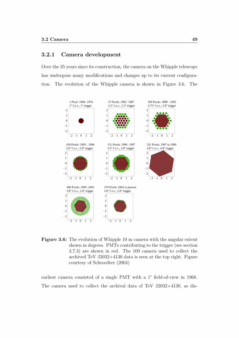
3.2 Camera 49

3.2.1 Camera development

Over the 35 years since its construction, the camera on the Whipple telescope

has undergone many modifications and changes up to its current configura-

tion. The evolution of the Whipple camera is shown in Figure 3.6. The

-2 -1 0 1 2

-2

-1

0

1

2

490 Pixels: 1999-20033.8° f.o.v., 2.6° trigger

-2 -1 0 1 2

-2

-1

0

1

2

379 Pixels: 2003 to present2.8° f.o.v., 2.6° trigger

-2 -1 0 1 2

-2

-1

0

1

2

109 Pixels: 1993- 19963.0° f.o.v., 2.8° trigger

-2 -1 0 1 2

-2

-1

0

1

2

151 Pixels: 1996-19973.5° f.o.v., 2.8° trigger

-2 -1 0 1 2

-2

-1

0

1

2

331 Pixels: 1997 to 19994.8° f.o.v., 4.8° trigger

-2 -1 0 1 2

-2

-1

0

1

2

1 Pixel: 1968-19761° f.o.v., 1° trigger

-2 -1 0 1 2

-2

-1

0

1

2

37 Pixels: 1982-19873.3° f.o.v., 2.3° trigger

-2 -1 0 1 2

-2

-1

0

1

2

109 Pixels: 1988- 19933.75° f.o.v., 2.8° trigger

Figure 3.6: The evolution of Whipple 10 m camera with the angular extentshown in degrees. PMTs contributing to the trigger (see section3.7.3) are shown in red. The 109 camera used to collect thearchived TeV J2032+4130 data is seen at the top right. Figurecourtesy of Schroedter (2004)

earliest camera consisted of a single PMT with a 1° field-of-view in 1968.

The camera used to collect the archival data of TeV J2032+4130, as dis-

3.3 Data Acquisition System 50

cussed in Chapter 6, was the 109 PMT camera used between 1988 and 1993.

This older camera consisted of an array of PMTs similar in design to the 379

PMT camera with several subtle differences. The older array consisted of 91

inner PMTs of diameter 29 mm, arranged in five concentric rings centered

on a central tube surrounded by a single ring of 18 tubes of diameter 50

mm, resulting in a total field-of-view of 3.75°. A detailed description of the

109 PMT camera can be found in Cawley et al. (1990). The current camera

configuration with a total of 490 pixels was initially installed in the autumn

of 1999 and was operated with 379 pixels from 2003 onwards.

3.3 Data Acquisition System

Signals from the PMT array are processed by the data acquisition system

built using the fast electronic CAMAC bus system of crates and modules

(Rose et al., 1995). A schematic of the system used is shown in Figure

3.7. Using this system, instructions and data are passed to a crate housing

several programmable electronic devices. Crate controllers manage the flow

of information by Ethernet to the work crates and the data acquisition system

computer. This computer passes instructions to the data acquisition system

devices through the crate controllers and receives data from the analogue to

digital converters (ADCs) and other equipment by means of a CAMAC data

buffer known as a list processor.

3.3.1 Amplification

The signals are transferred from the inner 379 PMTs to the pre-amplifiers

of the data acquisition system via RG58 coaxial cable. The amplifiers used

for the PMTs are LeCroy 612A amplifiers with a gain factor of ten. Of the

3.3 Data Acquisition System 51

ADCs

List

Proc

Tim

CFDs

PST

Adder

Mult.

Trigger

Gate

Generator

GPS

Clock

Gate Width

Discrim

Amplifer

Current

Monitor

Fibre optic

Coupler

Camera

CAMAC

BUS

Scal

Delay Cable

Pedestal

Trigger

Ethernet

Crate

Controller

DAQ

Computer

Scalers

Timing

Figure 3.7: Schematic representation of the data acquisition system for the490 PMT camera. PST refers to the pattern selection triggeras described in Section 3.3.3 and CFDs refer to the constantfraction discriminators.

3.3 Data Acquisition System 52

379 channels, 311 are used in the trigger system. The outer most PMTs are

not part of the trigger system as Cherenkov images on the outer edge of the

camera can be truncated. There are three outputs from each amplifier.

One output is AC coupled to the ADCs, but with a delay incorporated

via a length of coaxial cable to allow time for the trigger decision to be

made.

The signal from each inner PMT is passed through a constant fraction

discriminator.

The final output is coupled to the current monitor. See Section 3.6.5.

LeCroy 3420 constant fraction discriminators (CFDs) are used to determine

whether a PMT has fired. If the signal from a PMT rises above a preset

threshold, the discriminator will output a pulse of preset amplitude and du-

ration. The timing of the leading edge of the output signal is determined

using a constant fraction of the input signal, resulting in a more accurate

synchronisation of signal and trigger pulse than a standard fixed value dis-

criminator. The constant fraction discriminators have three outputs. One

set is fed into the single rate scalers. The single rate scalers count the number

of times individual tubes have fired. This information is used to monitor any

problems with specific tubes. The scalers are only read during a pedestal

event, see Section 3.3.4. The remaining constant fraction discriminator out-

puts are to the pattern selection trigger (PST) and to an adder which sums

the signals and outputs a pulse (proportional to the number of PMTs that

fired) directly to the multiplicity trigger.

3.3 Data Acquisition System 53

3.3.2 Multiplicity Trigger

The multiplicity trigger determines if the required number of tubes have fired

in order for data to be recorded. The required number of tubes is called the

multiplicity of the system. Generally the Whipple camera uses a three-fold

trigger. This trigger helps keep the amount of accidental triggers due to

background light down and provides a low time-jitter signal to initiate signal

integration by the ADCs.

3.3.3 Pattern Selection Trigger

The pattern selection trigger was developed to further reduce the number

of background events triggering the camera (Bradbury & Rose, 2002). The

pattern selection trigger uses the location of signals output from the constant

fraction discriminators to determine if the trigger is background related. As

described in 3.3.2, the multiplicity trigger operates when any three tubes are

above the preset threshold. The pattern selection trigger will only trigger if

the three tubes (assuming three-fold multiplicity) that triggered the multi-

plicity trigger are adjacent. This trigger system further reduces the chance

of background light triggering the camera. This in turn allows the system to

operate at a lower constant fraction discriminator threshold while at the same

time maintaining a reasonable trigger rate. Figure 3.8 shows an example of a

bias curve during the 2000 observing season. A bias curve is a plot of trigger

rate versus constant fraction discriminator threshold for the multiplicity trig-

ger and the pattern selection trigger and is used to determine the constant

fraction discriminators threshold for each season. In the example shown the

threshold was found to be 36 mV. As seen, the trigger rate increases from

a high constant fraction discriminator threshold to a low constant fraction

3.3 Data Acquisition System 54

20 30 40 50 60 70 8010

0

101

102

103

104

105

106

107

CFD Threshold (mV)

Trig

ger

Rat

e (H

z)

3−Fold Multiplicity3−Fold Pattern

2000 Season CFD Level36 mV

Figure 3.8: Bias curves of trigger rate vs. Constant fraction discriminatorthreshold for Multiplicity and Pattern Triggers.

3.3 Data Acquisition System 55

discriminator threshold. At high values the trigger rate is dominated by cos-

mic rays. As the threshold gets lower, the trigger rate increases rapidly. At

these lower values the trigger rate is dominated by random fluctuations in

the night sky. The constant fraction discriminator trigger is chosen to be

as low as possible without being in the regime dominated by the night sky

background. It can also be seen from the diagram how a lower threshold

level can be attained by using a pattern selection triggering system.

3.3.4 Pedestal Trigger

Since the PMT signals are AC coupled before they reach the ADCs, the effects

of the average night sky background current as well as other dark currents

are removed. However, positive and negative fluctuations from the average

current can occur in the 25 ns ADC integration time. These fluctuations must

be measured in order to characterise the background noise in the system.

This is achieved by injecting a constant “pedestal” current into the ADCs

along with the signal from the PMTs. The main requirement here is that

the size of the current is set so that the majority of the negative night sky

fluctuations will still result in a positive ADC signal when integrated over

the gate. The pedestal current level is usually set to produce a level of ∼ 20

digital counts which corresponds to the ADC output for zero input. When

the data are analysed the level of these pedestals must be determined and

then removed from the data leaving only the night sky fluctuations and any

Cherenkov signals.

To do this a pedestal event is artificially triggered by means of a global

positioning satellite (GPS) clock once every second and is tagged by the

data acquisition system to distinguish it from real events. It is assumed

that all the recorded ADC counts in these triggered images are due solely

3.3 Data Acquisition System 56

to night sky noise. By recording each pedestal event over the duration of a

28 minute run, the mean amplitude of the injected pedestal for each channel

can be calculated. The RMS deviation from the mean is also calculated and

is called the “pedestal variance” (“pedvar”). This value is representative of

the size of the average sky fluctuation for each channel.

From the pedvar values the median is found. Each PMT’s pedvar is then

compared with the median value and if found to be too large (> 1.5 times

median value), then it is assumed that the tube had a star or bright region

of the sky in its field of view during the observation run. In this case the

analysis software ignores this channel so it does not influence the outcome of

the analysis result. Similarly, if the pedvar of a channel is found to be too

low (< 0.6 times median value), it is also disabled by in the analysis routines

as the tube may actually have been switched off or not functioning properly.

3.3.5 Data Read out and Recording

If all the trigger requirements are met, the signal is sent into the gate gen-

erator, which in turn outputs a negative square pulse to the ADCs via a

discriminator. The ADCs are LeCroy 10 bit 2249 modules. Even though

Cherenkov pulses are about 5 ns in duration, the width of the square pulse

is set to ∼ 25 ns. This allows for dispersion of the signal introduced by

the electronics. The PMT signal is integrated over the duration of the gate

signal.

After signal integration the data is transferred via the CAMAC bus to

the list processor. The list processor is essentially a data buffer between the

CAMAC crates and the data acquisition computer. This buffer also stores

timing and scaler information until the data acquisition computer is ready

to receive the data. The data acquisition computer operates under VMS and

3.4 Data Analysis Techniques 57

controls each observation run. The final task of the of the data acquisition

computer is to record all data, including tracking, timing and monitoring

information, to the hard drive. These data are then archived for off-line

analysis at a later date.

3.4 Data Analysis Techniques

Previous sections have detailed the physics behind EAS, the instruments used

to detect the Cherenkov flash caused by EAS, and the observational methods

used as part of the imaging atmospheric Cherenkov technique. Once the

events, that have triggered the camera, have been recorded and stored by

the data acquisation system it is then the task of the analysis routines to

identify and differentiate the γ-ray events from the large number of hadronic

events. This section describes the remaining element used in the imaging

atmospheric Cherenkov technique; analysis and identification of Cherenkov

images.

3.4.1 Data Calibration

Before the data can be analysed they must be prepared for analysis via the

following steps:

Pedestal Subtraction: the removal of the positive offset added to the

ADC outputs as described in Section 3.3.4.

Flat Fielding: Since each PMT has a slightly different gain, it is nec-

essary to scale the signals recorded in each tube accordingly so PMTs

with larger gains do not distort the final analysed image. This is done

using the nitrogen lamp as discussed in Section 3.6.3.

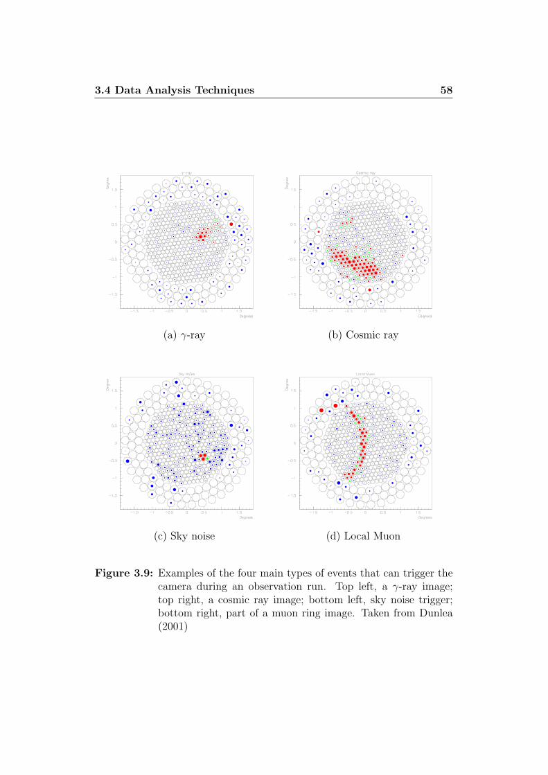
3.4 Data Analysis Techniques 58

(a) γ-ray (b) Cosmic ray

(c) Sky noise (d) Local Muon

Figure 3.9: Examples of the four main types of events that can trigger thecamera during an observation run. Top left, a γ-ray image;top right, a cosmic ray image; bottom left, sky noise trigger;bottom right, part of a muon ring image. Taken from Dunlea(2001)

3.4 Data Analysis Techniques 59

Noise padding. During the course of an observation run the sky bright-

ness of the ON (the source being observed) or OFF (the control ob-

servation) region (see Section 3.5) can vary significantly. This means

pedestal deviations can differ accordingly and can introduce a bias, dis-

torting the results of the analysis procedure. To rectify this problem

the noise levels must be equalised in the ON and the OFF runs. To

do this artificial noise is added to the data from the darker of the two

sky regions.

Finally, before parameterisation, the images must be cleaned. Once

the above processes are complete, what is left is an image of the signal

due to the Cherenkov flash and noise due to the night sky background.

Hence, before analysis, the night sky background element of the signal

must be removed as best as possible. This is achieved by the follow-

ing method of applying picture and boundary thresholds. Picture and

boundary thresholds are what define the boundaries of the image and

are defined as :

– The picture threshold is defined as the multiple of the RMS pedestal

deviation which the tube must exceed to be part of the picture.

– The boundary threshold is defined as the multiple which tubes

adjacent to the picture must exceed to be part of the boundary.

Picture and boundary thresholds are optimised and set at 4.25σ

and 2.25σ respectively (Punch et al., 1991).

This project utilised two different analysis techniques in an attempt to

correctly identify the Cherenkov flash induced by a high energy γ-ray photon;

Supercuts and Kernel analysis. Both of these techniques are very successful

in rejecting nearly 100% of noise events while retaining over 50% of genuine

3.4 Data Analysis Techniques 60

Width

Length

Centre of field of view

α

Azwidth

Distance

Miss

Figure 3.10: The Hillas parameters.

γ-rays (Fegan, 1997; Moriarty & Samuelson, 2000). The Supercuts technique

was used in conjunction with the deconvolution of Cherenkov images while

a Kernel analysis was performed on archival Whipple data for the first time.

3.4.2 Standard Image Analysis (Supercuts)

The standard analysis software used by the VERITAS Collaboration, known

as Supercuts, uses moment fitting routines to fit an ellipse to the recorded

Cherenkov images. Generally, a Cherenkov image from a γ-ray induced air

shower will appear as an elliptical image pointing towards the centre of the

field of view of the PMT array. Figure 3.9(a) shows a typical, uncleaned,

Cherenkov image from a γ-ray induced air shower. Figure 3.9 (b), (c) and (d)

illustrate typical hadronic events, noise events and a single muon event. It is

these events shown in Figure 3.9 (b),(c) and (d), that contribute to over 99%

of events recorded by imaging atmospheric Cherenkov telescopes. From the

diagram the subtle differences between each of the events can clearly be seen.

Hillas (1985) derived a moment fitting procedure to try and exploit these

3.4 Data Analysis Techniques 61

Length∗ The RMS spread of light along themajor axis of the ellipse (longitudi-nal development of the shower).

Width∗ The RMS spread of light along theminor axis of the ellipse (lateral de-velopment of the shower).

Azwidth∗ The RMS Spread of light perpendic-ular to the line connecting the imagecentroid with the centre of the fieldof view; a measure of the shape andorientation of the image.

Miss∗ The perpendicular distance betweenthe major axis of the image and thecentre of the field of view.

Distance∗ The distance between the centroid ofthe image and the centre of the fieldof view.

Alpha The angle between the major axis ofthe ellipse and a line joining the cen-troid of the ellipse to the centre ofthe field of view.

Frac3 ∗ Fraction of the total light in theimage contained in the three high-est tubes; used to eliminate eventscaused by sky noise and particlesphysically passing through the cam-era.

Size The total number of digital countsin all of the tubes; a number propor-tional to the energy of the primaryparticle.

Asymmetry A measure of how symmetric the im-age is.

Max1, Max2 &Max3

The signals in the highest threetubes.

Length/Size A measure of the compactness of theimage in relation to its total lightcontent; helps to eliminate back-ground due to local muons.

Table 3.2: The Hillas Parameters. ∗ Denotes the original six Hillas param-eters.

3.4 Data Analysis Techniques 62

differences and in turn provide a means to differentiate between unwanted

noise events and true γ-ray induced events.

Knowing that images produced by γ-ray induced showers, from sources lo-

cated at the centre of the field of view, resemble compact ellipsoids with their

major axes pointing towards the centre of the field of view, Hillas defined a

set of six parameters to describe the shape and orientation of a Cherenkov

image (illustrated in Figure 3.10). Table 3.2 defines the original set of Hillas

parameters and additional parameters introduced to increase the γ-ray se-

lection efficiency. A full description of the moment fitting technique can be

found in Reynolds et al. (1993).

By choosing an appropriate range of selection cuts to each of the pa-

rameters listed in Table 3.2, it is possible to reject over 98% of the cosmic

ray background whilst keeping ∼ 60% of the γ-ray events. Since they were

first developed, the Hillas parameters have evolved to adapt to a changing

instrument.

A variant of the original Hillas parameters, Supercuts has since become

the most successful selection mechanism used by the VERITAS Collabora-

tion. Having been optimised using observations of the Crab Nebula (Punch

et al., 1991), the VERITAS Collaboration has since used Supercuts in the

discovery of several new sources (Horan et al., 2002; Holder et al., 2003).

The Supercuts selection criteria as used by the VERITAS Collaboration are

listed in Table 3.3.

3.4.3 Kernel Analysis

In addition to the standard Supercuts analysis technique, the Kernel multi-

variate analysis technique was applied to a portion of the work in this project

as will be discussed in Chapter 6. Supercuts essentially classifies events, each

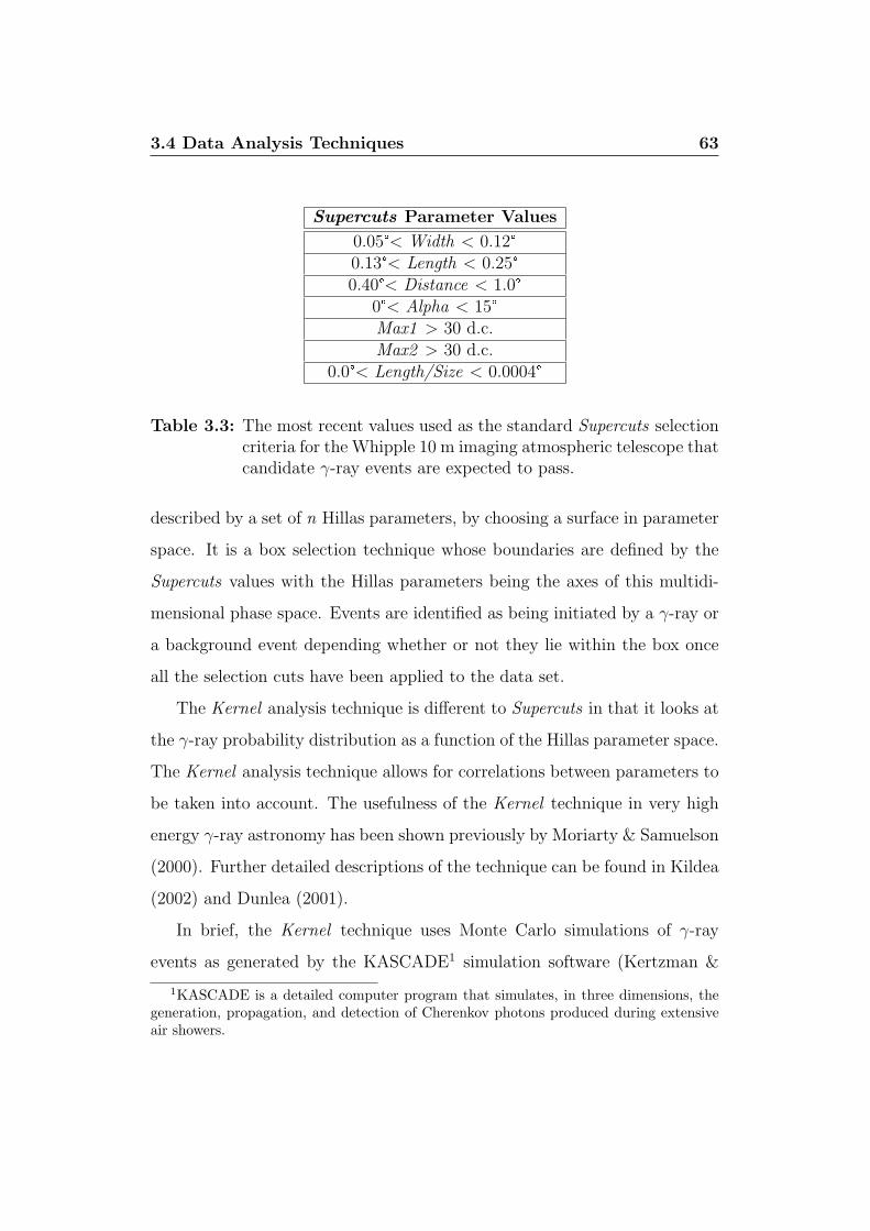
3.4 Data Analysis Techniques 63

Supercuts Parameter Values

0.05°< Width < 0.12°0.13°< Length < 0.25°0.40°< Distance < 1.0°

0°< Alpha < 15°Max1 > 30 d.c.Max2 > 30 d.c.

0.0°< Length/Size < 0.0004°

Table 3.3: The most recent values used as the standard Supercuts selectioncriteria for the Whipple 10 m imaging atmospheric telescope thatcandidate γ-ray events are expected to pass.

described by a set of n Hillas parameters, by choosing a surface in parameter

space. It is a box selection technique whose boundaries are defined by the

Supercuts values with the Hillas parameters being the axes of this multidi-

mensional phase space. Events are identified as being initiated by a γ-ray or

a background event depending whether or not they lie within the box once

all the selection cuts have been applied to the data set.

The Kernel analysis technique is different to Supercuts in that it looks at

the γ-ray probability distribution as a function of the Hillas parameter space.

The Kernel analysis technique allows for correlations between parameters to

be taken into account. The usefulness of the Kernel technique in very high

energy γ-ray astronomy has been shown previously by Moriarty & Samuelson

(2000). Further detailed descriptions of the technique can be found in Kildea

(2002) and Dunlea (2001).

In brief, the Kernel technique uses Monte Carlo simulations of γ-ray

events as generated by the KASCADE1 simulation software (Kertzman &

1KASCADE is a detailed computer program that simulates, in three dimensions, thegeneration, propagation, and detection of Cherenkov photons produced during extensiveair showers.

3.4 Data Analysis Techniques 64

Sembroski, 1994) along with real background events to define a probability

surface where events on one side of the surface have a high probability of

being γ-rays and events on the other side are predominantly background

events. For a point p in parameter space this surface is calculated using the

log-likelihood function:

log (R(p)) = log

(fγ(p)

fb(p)

)(3.1)

where fγ(p) is the γ-ray probability distribution as a function of location, p, in

Hillas parameter space and fb(p) is the corresponding background probability

distribution function. That is, f γ(p) is the likelihood the real data event

being analysed corresponds to a γ-ray and f b(p) is the likelihood it is a

background event. The calculation of these distributions is the key to the

Kernel analysis technique (Dunlea et al., 2001). log(R(p)) gives an indication

as to the identity of each event in a data set. A suitable log(R(p)), or cut

value, may be chosen such that any real events with a score lower than this

are rejected and assumed to be background events.

Since γ-ray events and background events populate this parameter space

in a complex way, it is not possible to describe their probability density dis-

tribution analytically in terms of a simple function, although attempts have

been made Samuelson (1999). The simplest probability density estimator is

a histogram. However a histogram in this instance is not ideal since each

cell has a fixed width, and a limited range, as well as cell boundary discon-

tinuities (Hand, 1982). In an attempt to remove these problems, the Kernel

convolves each data point with a point-spread function and sums the results,

producing a smooth, continuous approximation to the probability distribu-

tion. The basic Kernel estimator is found using a set of N γ simulations and

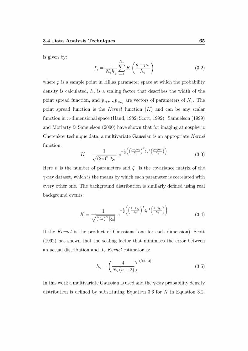
3.4 Data Analysis Techniques 65

is given by:

fγ =1

Nγhnγ

Nγ∑i=1

K

(p− pγi

hγ

)(3.2)

where p is a sample point in Hillas parameter space at which the probability

density is calculated, hγ is a scaling factor that describes the width of the

point spread function, and pγ1 ,...,pγNγare vectors of parameters of Nγ. The

point spread function is the Kernel function (K ) and can be any scalar

function in n-dimensional space (Hand, 1982; Scott, 1992). Samuelson (1999)

and Moriarty & Samuelson (2000) have shown that for imaging atmospheric

Cherenkov technique data, a multivariate Gaussian is an appropriate Kernel

function:

K =1√

(2π)n |ξγ|e− 1

2

((p−pγi

hγ

)Tξ−1γ

(p−pγi

hγ

))

(3.3)

Here n is the number of parameters and ξγ is the covariance matrix of the

γ-ray dataset, which is the means by which each parameter is correlated with

every other one. The background distribution is similarly defined using real

background events:

K =1√

(2π)n |ξb|e− 1

2

((p−pbi

hb

)T

ξ−1b

(p−pbi

hb

))

(3.4)

If the Kernel is the product of Gaussians (one for each dimension), Scott

(1992) has shown that the scaling factor that minimises the error between

an actual distribution and its Kernel estimator is:

hγ =

(4

Nγ (n + 2)

)1/(n+4)

(3.5)

In this work a multivariate Gaussian is used and the γ-ray probability density

distribution is defined by substituting Equation 3.3 for K in Equation 3.2.

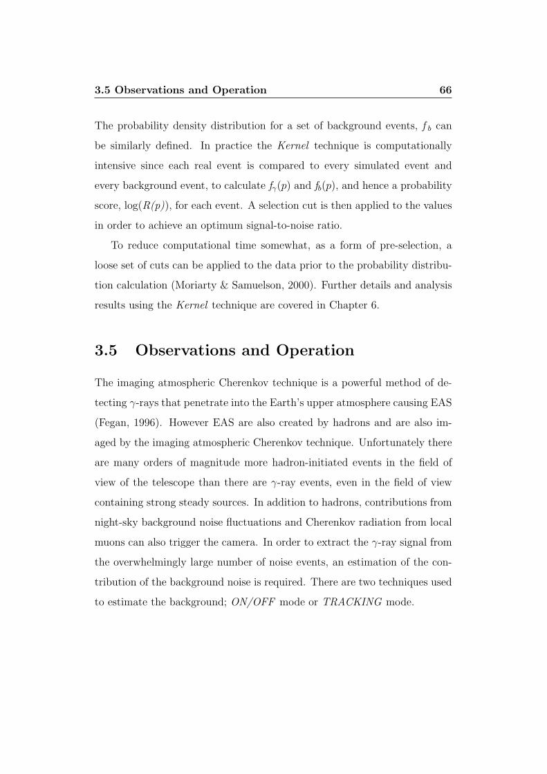
3.5 Observations and Operation 66

The probability density distribution for a set of background events, f b can

be similarly defined. In practice the Kernel technique is computationally

intensive since each real event is compared to every simulated event and

every background event, to calculate fγ(p) and fb(p), and hence a probability

score, log(R(p)), for each event. A selection cut is then applied to the values

in order to achieve an optimum signal-to-noise ratio.

To reduce computational time somewhat, as a form of pre-selection, a

loose set of cuts can be applied to the data prior to the probability distribu-

tion calculation (Moriarty & Samuelson, 2000). Further details and analysis

results using the Kernel technique are covered in Chapter 6.

3.5 Observations and Operation

The imaging atmospheric Cherenkov technique is a powerful method of de-

tecting γ-rays that penetrate into the Earth’s upper atmosphere causing EAS

(Fegan, 1996). However EAS are also created by hadrons and are also im-

aged by the imaging atmospheric Cherenkov technique. Unfortunately there

are many orders of magnitude more hadron-initiated events in the field of

view of the telescope than there are γ-ray events, even in the field of view

containing strong steady sources. In addition to hadrons, contributions from

night-sky background noise fluctuations and Cherenkov radiation from local

muons can also trigger the camera. In order to extract the γ-ray signal from

the overwhelmingly large number of noise events, an estimation of the con-

tribution of the background noise is required. There are two techniques used

to estimate the background; ON/OFF mode or TRACKING mode.

3.5 Observations and Operation 67

ON/OFF

In ON/OFF mode a putative source of VHE γ-rays is first observed for 28

minutes. This is the ON run and is followed by another 28 minute run

with the telescope position offset by 30 minutes in right ascension from the

ON -source position. This is the OFF run or a region of sky with no VHE

γ-ray signal. Together the ON/OFF runs are called pairs. The OFF run can

then be used as an estimate of the background in the ON run. Assuming a

Poissonian noise distribution, the significance2, σ, of the excess ON -source

γ-ray events above the background of OFF -source events can be calculated

using the Li & Ma (1983) method

σ =ON −OFF√ON + OFF

(3.6)

where ON is the number of events that pass the γ-ray selection criteria in

the ON -source run and OFF is the number passing in the OFF -source run.

A signal of 5σ of more, along with an equivalent result from an independent

group, is considered as a source detection (Weekes, 1999). The corresponding

γ-ray rate and its error, expressed in γ-ray events per minute, is calculated

using

Rate =ON −OFF

time±√

ON + OFF

time(3.7)

where time is the total time spent ON -source. The ON/OFF mode of ob-

servations has been in use now for many years and is accepted as an effective

method for use with the imaging atmospheric Cherenkov technique. It does

2The ratio of the signal to its standard deviation

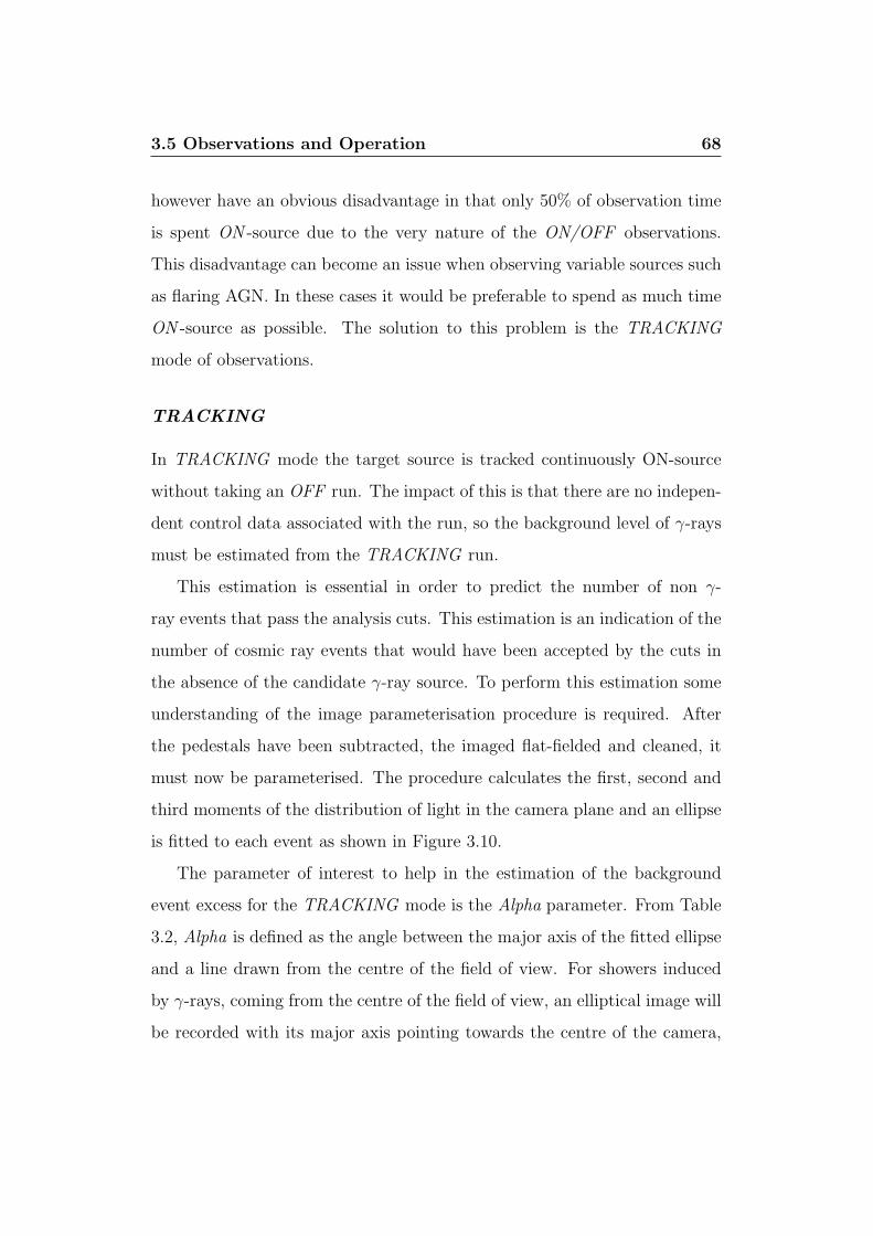
3.5 Observations and Operation 68

however have an obvious disadvantage in that only 50% of observation time

is spent ON -source due to the very nature of the ON/OFF observations.

This disadvantage can become an issue when observing variable sources such

as flaring AGN. In these cases it would be preferable to spend as much time

ON -source as possible. The solution to this problem is the TRACKING

mode of observations.

TRACKING

In TRACKING mode the target source is tracked continuously ON-source

without taking an OFF run. The impact of this is that there are no indepen-

dent control data associated with the run, so the background level of γ-rays

must be estimated from the TRACKING run.

This estimation is essential in order to predict the number of non γ-

ray events that pass the analysis cuts. This estimation is an indication of the

number of cosmic ray events that would have been accepted by the cuts in

the absence of the candidate γ-ray source. To perform this estimation some

understanding of the image parameterisation procedure is required. After

the pedestals have been subtracted, the imaged flat-fielded and cleaned, it

must now be parameterised. The procedure calculates the first, second and

third moments of the distribution of light in the camera plane and an ellipse

is fitted to each event as shown in Figure 3.10.

The parameter of interest to help in the estimation of the background

event excess for the TRACKING mode is the Alpha parameter. From Table

3.2, Alpha is defined as the angle between the major axis of the fitted ellipse

and a line drawn from the centre of the field of view. For showers induced

by γ-rays, coming from the centre of the field of view, an elliptical image will

be recorded with its major axis pointing towards the centre of the camera,

3.5 Observations and Operation 69

i.e. a small value of Alpha. For each run the number of Alpha values can be

binned according to their value and a histogram can be plotted. The “Alpha

plot” for a positive source will generally have a large excess with small values

of the Alpha parameter.

With TRACKING runs, the background level of γ-ray like events in the

field of view can be estimated by using a pool of OFF runs known as “dark-

field data” and the shape of the resulting Alpha plot is characterised. To do

this, a large database of darkfield data is analysed and an approximately flat

Alpha plot is obtained, as expected when no γ-rays are present.

In reality this Alpha plot isn’t completely flat and any fluctuations seen

are due to the finite size of the pixels and truncation effects due to events

being imaged at the edge of the field of view. In particular, events with an

Alpha value > 65° are sensitive to truncation effects and hence are not used

in the determination of the level of background. Generally the Alpha plot is

flat up 65°.As mentioned, γ-ray events from a source located at the centre of the field

of view will tend to have lower values of Alpha, i.e. < 20°, so the distribution

above 20° is assumed not to be associated with any γ-ray source. With

these Alpha limits in mind, the range of Alpha values between 20° and 65°is representative of the background level of γ-ray like events in the field of

view. Using darkfield data, a ratio is calculated to scale the number of events

between 20° and 65° to the number that pass the standard Alpha cut in the

darkfield data. This ratio is the “tracking ratio” (ρ) and is then used to scale

the 20°and 65°region for the TRACKING run, to estimate the background

level of events passing all cuts. The tracking ratio is calculated as follows:

ρ±∆ρ =Nsource

Ncontrol

±√

Ncontrol

N2source

+N2

control

N3source

(3.8)

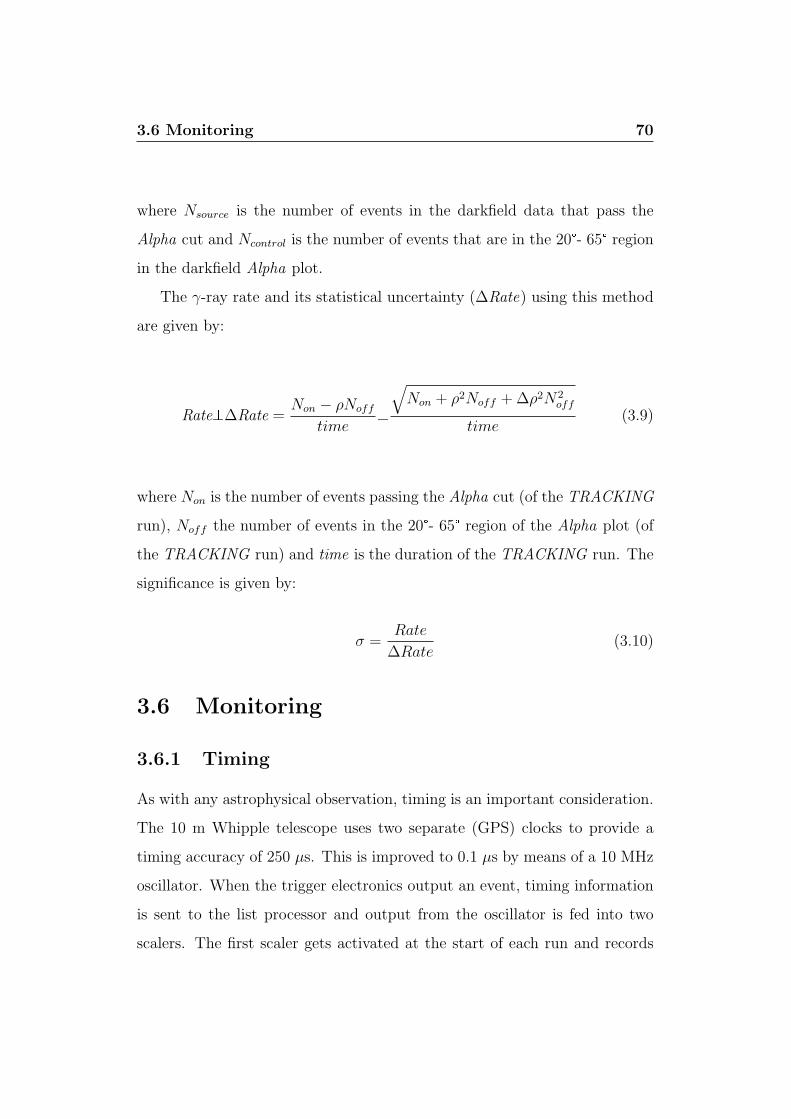
3.6 Monitoring 70

where Nsource is the number of events in the darkfield data that pass the

Alpha cut and Ncontrol is the number of events that are in the 20°- 65° region

in the darkfield Alpha plot.

The γ-ray rate and its statistical uncertainty (∆Rate) using this method

are given by:

Rate±∆Rate =Non − ρNoff

time±

√Non + ρ2Noff + ∆ρ2N2

off

time(3.9)

where Non is the number of events passing the Alpha cut (of the TRACKING

run), Noff the number of events in the 20°- 65° region of the Alpha plot (of

the TRACKING run) and time is the duration of the TRACKING run. The

significance is given by:

σ =Rate

∆Rate(3.10)

3.6 Monitoring

3.6.1 Timing

As with any astrophysical observation, timing is an important consideration.

The 10 m Whipple telescope uses two separate (GPS) clocks to provide a

timing accuracy of 250 µs. This is improved to 0.1 µs by means of a 10 MHz

oscillator. When the trigger electronics output an event, timing information

is sent to the list processor and output from the oscillator is fed into two

scalers. The first scaler gets activated at the start of each run and records

3.6 Monitoring 71

the elapsed time. The second scaler is also activated at the start of the run.

However it only operates when the trigger gate is open, and thus provides a

measure of the live time of the system.

3.6.2 Tracking

The Whipple 10 m telescope has an Alt-Azimuth mount. Each axis is driven

independently by a variable speed motor with a resolution of 0.01°. The

mount has a slew rate of 1° per second and has an azimuth range of 270°in both east and west directions and an elevation range of 0° to 90°. The

pointing of the telescope is controlled by a computer located in the control

room. The equatorial coordinates of a given source are stored in a database

and an integrated software algorithm constantly calculates the altitude and

azimuth of the source by reference to local sidereal time. Sidereal time is

obtained from a remote Network Time Server. This enables the telescope to

continuously track the source in the sky.

As a safety measure, there are limit switches to prevent the telescope

from moving beyond its range, both in elevation and azimuth. There is a

software limit that, when reached, instructs the drive controllers to stop. In

the case of a software failure, there are also hardware limit switches installed

on the telescope mount that will stop the drive motors.

Tracking accuracy is normally checked several times during a nights ob-

servation by lining up the telescope with a guide star. This is known as a

“pointing check”. Once the telescope has centered the guide star, the cur-

rents in the inner seven PMTs are monitored. If the pointing is accurate then

the central PMT will have the largest current reading, while the remaining

six PMTs will have some overflow of excess current.

3.6 Monitoring 72

3.6.3 Nitrogen Lamp

A blue nitrogen arc lamp, used to calibrate the PMT camera, is located at

the centre of the telescope dish. At the beginning of every night the lamp is

activated and pulses at high frequency, providing uniform illumination across

the camera. The data acquisation system starts this “nitrogen run” which

lasts for one minute. During this time the camera is triggered by a large

number of artificial events, which in turn are used to calculate the gain of

each tube relative to the average gain. These gains are then applied later

in the analysis of the data in a process known as “flat fielding”, where each

PMT output is scaled by the appropriate gain value.

3.6.4 High Voltage System

In order for the PMT camera to operate, a high voltage system is required

to power each PMT. Three LeCroy high voltage (HV) modules supply the

required HV to all PMTs. The HV modules are located on the telescope

counterweights and are operated remotely, via Ethernet, from the control

room. Here a computer monitors the voltage settings on each tube and can,

if required, shut down individual PMTs. Individual PMT HV settings can

also be adjusted by using the camera-related software in the control room.

3.6.5 Current Monitor

As well as monitoring the HV applied to the PMT, the anode current of

each PMT is also measured and monitored in parallel with the main data

acquisition. After the amplification stage, the PMT signals are sent to the

current monitor. The ADCs in the current monitor have an integration time

much greater than the ADCs in the data acquisition system allowing the

3.6 Monitoring 73

presence of steady back ground light to be seen. This is particularly useful

for detecting stars that may be in the field of view during a data run.

Information on PMT currents is sent to the HV control program via a

serial link and a colour coded graphical display detailing tube current status,

as well as HV information, is output to a screen. If there is a problem with

any of these systems the telescope operator is alerted and can act accord-

ingly. The tube current display is particularly useful for indicating when a

star enters the field-of-view. The observer can then temporally disable any

affected tubes thus avoiding damage from excess current.

3.6.6 Weather Monitoring

As with most other types of astronomy, good weather conditions are of the

utmost importance to γ-ray astronomy. With this in mind, there are several

weather monitoring tools available to measure observing conditions during

the course of a night’s observations. Each night the atmospheric conditions

are recorded in the observer log sheet with conditions rated as A,B or C, cor-

responding to very good, fair, or poor weather conditions. During 2001/2002,

a weather station and far-infrared (FIR) pyrometer were installed and tested

on the 10 m site. The weather station measured temperature, wind speed

and humidity. The pyrometer gave a further indication of sky clarity by

measuring the night-sky temperature. Clouds passing within the FOV pro-

duce an increase in the reported pyrometer temperature. This temperature

increase is proportional to the height, thickness and water content of the

cloud. With no cloud present, the temperature decreases to the quiescent

level, which is almost entirely dependent upon the water vapour content in

the atmosphere above the detector (Dowdall, 2003). The weather station

and FIR pyrometer have since been installed at base camp for use with the

3.6 Monitoring 74

VERITAS array. Currently, weather information is obtained from a weather

station at the nearby 60” optical telescope and from satellite information

available from several weather internet sites.

A further tool for monitoring sky conditions, albeit a crude one, is an

optical camera. An Electrim EDC1000L Charged-Coupled Device (CCD),

coupled with a 25mm f/0.85 Fujinon lens is mounted on the telescope next

to the focus box, with its optic axis close to and parallel to the optic axis of

the reflector. This camera has several other uses too. It can also be used as

an independent check of telescope pointing and also gives a further warning

of any bright stars in the field of view. The camera has a field of view of

8°, and, depending on exposure time, images captured are displayed in the

control room and are updated every ten to twenty seconds.

Chapter 4

VHE γ-ray Sources and

Ground Based Detectors

4.1 VHE γ-ray Sources

At present no complete sky survey exists at TeV energies, although progress

in this area is being made. A map of the known sources including the most

recent detections in this energy regime is represented in Figure 4.1. The list of

known sources has more than doubled since the newer imaging atmospheric

Cherenkov instruments have come on line. It is expected that the list of

sources in the northern hemisphere will grow further when VERITAS starts

to return scientific results in the coming months along with the expanding

HESS catalogue of sources in the southern skies. Of the sources detected,

each source is classified as belonging to a particular type or class, due to the

nature of the emission from the object. Therefore, a variety of production

models have been published that describe the different types of γ-ray emis-

sion from these objects. This range of sources include galactic sources such

as supernova remnants (SNRs), and the related pulsar wind nebulae (PWN)

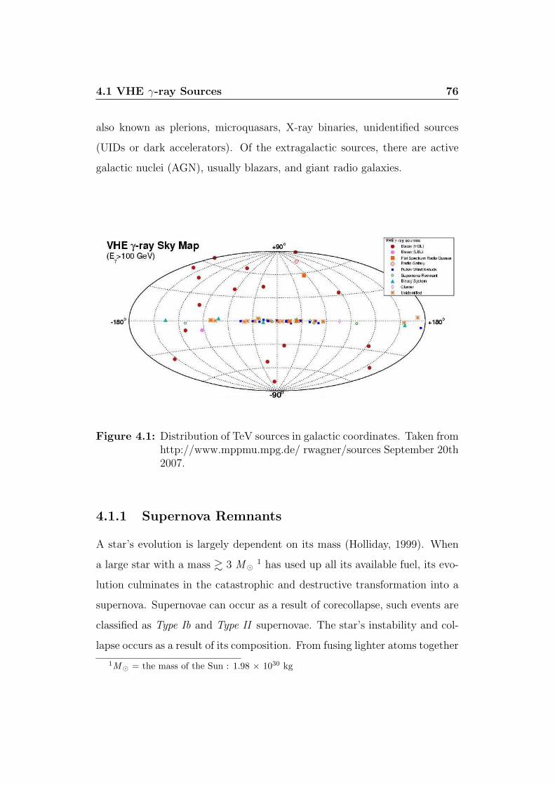
4.1 VHE γ-ray Sources 76

also known as plerions, microquasars, X-ray binaries, unidentified sources

(UIDs or dark accelerators). Of the extragalactic sources, there are active

galactic nuclei (AGN), usually blazars, and giant radio galaxies.

Figure 4.1: Distribution of TeV sources in galactic coordinates. Taken fromhttp://www.mppmu.mpg.de/ rwagner/sources September 20th2007.

4.1.1 Supernova Remnants

A star’s evolution is largely dependent on its mass (Holliday, 1999). When

a large star with a mass & 3 M¯ 1 has used up all its available fuel, its evo-

lution culminates in the catastrophic and destructive transformation into a

supernova. Supernovae can occur as a result of corecollapse, such events are

classified as Type Ib and Type II supernovae. The star’s instability and col-

lapse occurs as a result of its composition. From fusing lighter atoms together

1M¯ = the mass of the Sun : 1.98 × 1030 kg

4.1 VHE γ-ray Sources 77

for millions of years the star has created an ever-increasing amount of heavier

atoms. This process, while releasing nuclear energy in a very efficient man-

ner, is ultimately reliant upon the stars quantity of lighter elements. Once

this supply is exhausted the stars huge mass can no longer be supported by

the dwindling release of nuclear energy. The star succumbs to its own gravity

and so contracts. Eventually the core is no longer stable against inverse beta

decay. This results in the rapid removal of electrons from the electron gas

causing the core to collapse. Tremendous shock waves are generated and the

energy released, a large fraction of which is in the form of neutrinos, causes

the outside layers of the star to be ejected violently away from the core into

space. Approximately 1044 J is transferred as kinetic energy to the rapidly

moving ejecta.

Supernovae can also occur from binary star systems containing a white

dwarf and a red giant. Such Type Ia events arise from the white dwarf accret-

ing material from the companion. The dwarf’s mass and subsequent internal

pressure increase until reaching a critical density (1.4 M¯) resulting in the

uncontrollable fusion of its carbon and oxygen. The thermonuclear explosion

of the entire white dwarf releases Iron and other heavier elements into the

interstellar medium. A type Ia supernova is recognised by the absence of

hydrogen and the presence of elements such as silicon and sulfur in its spec-

trum. Since all Type Ia events are of similar magnitude they can be used as

precise ‘standard candles’ to measure the distances to their host galaxies.

Supernova explosions have durations of the order of seconds, and are only

expected to occur around once every 20 years in our galaxy. The gaseous

cloud, composed from the constituents of the former star is termed a Su-

pernova Remnant (SNR). If there remains a core of the original star, it can

continue to be quite active. If conditions are right the immediate aftermath

4.1 VHE γ-ray Sources 78

of a supernova may result in a rapidly rotating, highly magnetised, sphere

of neutrons known as a pulsar, and the supernova remnant or the remaining

nebula. (Note, not all supernovae result in the creation of a neutron star.

For example, the supernova remnant Cassiopeia A has no known associated

neutron star or pulsar.) The supernova remnant is enclosed by an expanding

shock wave that consists of ejected stellar material expanding from the ex-

plosion, and the interstellar material it sweeps up and accelerates along the

way..

There are two main types of SNR: a shell-type SNR (spherical shell) and

a plerion that has a filled centre containing a pulsar (Weiler, 1978). It is also

possible that the SNR has both a shell and plerionic component. The most

famous and most studied SNR is the Crab Nebula. It is a plerion in which the

high-energy electrons emit synchrotron radiation from radio energies to X-ray

energies, and the production of VHE γ-rays via inverse Compton scattering.

Salvati (1973) suggests that the filled interior is constantly replenished by

the conversion of the energy outflow from the pulsar into magnetic energy

and relativistic particles. As electrons are being continually injected into

the nebula, from the pulsar, and then travel through the inner magnetic

field, radio to X-ray synchrotron radiation is emitted. Inverse Compton

scattering of the synchrotron electrons on the ambient photons generates the

TeV emission (Blumenthal & Gould, 1970). Figure 4.2 from Aharonian &

Atoyan (1998b)shows the spectral energy distribution of the Crab Nebula

and two peaks can be seen that are representative of both types of emission.

VHE γ-ray emission from the Crab Nebula was first reported the 9σ level

after 60 hours of observations by the Whipple Observatory between 1987 and

1988 (Weekes et al., 1989). The Crab Nebula has since become the standard

candle for VHE astronomy (in the northern hemisphere) due to its continuous

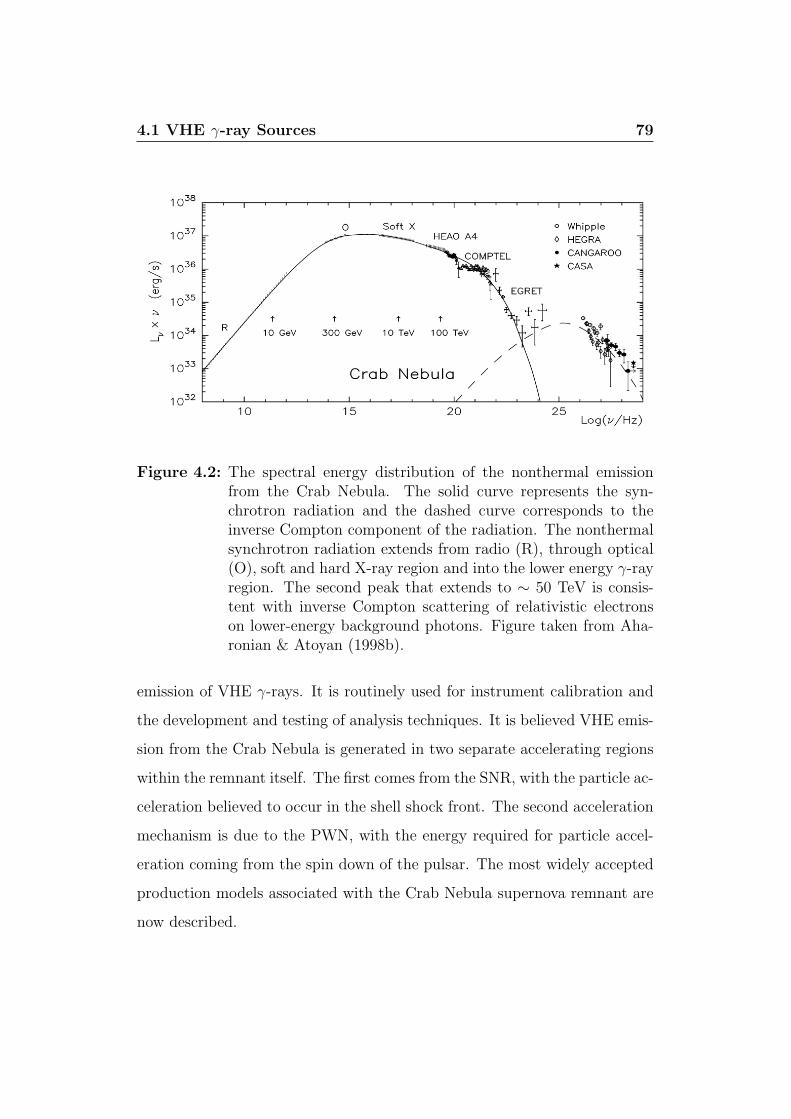
4.1 VHE γ-ray Sources 79

Figure 4.2: The spectral energy distribution of the nonthermal emissionfrom the Crab Nebula. The solid curve represents the syn-chrotron radiation and the dashed curve corresponds to theinverse Compton component of the radiation. The nonthermalsynchrotron radiation extends from radio (R), through optical(O), soft and hard X-ray region and into the lower energy γ-rayregion. The second peak that extends to ∼ 50 TeV is consis-tent with inverse Compton scattering of relativistic electronson lower-energy background photons. Figure taken from Aha-ronian & Atoyan (1998b).

emission of VHE γ-rays. It is routinely used for instrument calibration and

the development and testing of analysis techniques. It is believed VHE emis-

sion from the Crab Nebula is generated in two separate accelerating regions

within the remnant itself. The first comes from the SNR, with the particle ac-

celeration believed to occur in the shell shock front. The second acceleration

mechanism is due to the PWN, with the energy required for particle accel-

eration coming from the spin down of the pulsar. The most widely accepted

production models associated with the Crab Nebula supernova remnant are

now described.

4.1 VHE γ-ray Sources 80

SNR - acceleration in the Shell Shock Front

Cosmic rays are most likely accelerated by SNRs in the shock waves (Section

4.1.1) created by the initial supernova explosion (Bell, 1978; Drury et al.,

1994). These shock waves can last for thousands of years after the supernova

occurs. After the explosion, the shock waves propagate into interstellar space

and can be seen as the expanding shells of gas and debris of SNRs. Fermi ac-

celeration, also known as diffusive shock acceleration, is the acceleration that

charged particles undergo when reflected by a magnetic mirror. First-order

Fermi (Fermi-I) acceleration is thought to be the main mechanism by which

charged particles gain energy beyond the thermal energy in astrophysical

shock waves (Ellison et al., 1990; Reynolds & Ellison, 1992). Shock waves

can have magnetic inhomogeneities both preceding and following them. If a

charged particle traveling through the shock wave (upstream) encounters a

moving change in the magnetic field, it can be reflected back (downstream)

through the shock at an increased velocity. If a similar process occurs in

the opposite direction, the particle will again be accelerated and gain energy.

Figure 4.3 illustrates this mechanism of shock acceleration.

This type of acceleration is a possible candidate model that could be used

to explain shock acceleration of hadrons up to energies 100 TeV (Jones et al.,

1998). Fermi acceleration occurs with

dE

dt∝ νE (4.1)

where E is the energy of the particle being accelerated and ν is the velocity

of the upstream region of the shock relative to the downstream region. As

the shock wave moves out into interstellar space it gathers mass. If typical

interstellar density is 1 proton cm−3, then it will take ∼ 103 years for 10

4.1 VHE γ-ray Sources 81

ShockedRegion

CoreRemnant

FrontShock

Acceleratedparticle

ParticleSwept-up

Expanding

Figure 4.3: First-order Fermi acceleration by the shock wave of a supernovaremnant. Figure taken from Dunlea (2001).

M¯ of material moving at 5000 km s−1 to gather its own mass of interstellar

material (Gaisser, 1990). This period of time is when the shock is thought to

be most efficient at accelerating particles and is known as the Sedov Phase

and can last until the shock is up to 104 to ∼ 105 years old. High-energy

protons accelerated to very high energies in the shock region would interact

with nuclei in the Crab Nebula to create secondary particles, including π0

particles, which then decay creating VHE γ-rays.

Pulsar Emission Models

It is thought that pulsed emission from pulsars comes from the slowing of a

spinning neutron star as it loses angular momentum. Developing ideas first

proposed by Pacini (1967) and Gold (1968), Goldreich & Julian (1969) have

shown that, for a spinning neutron star in a vacuum, huge surface electric

4.1 VHE γ-ray Sources 82

fields (as big as 6 × 1010 V m−1) would exist parallel to the magnetic field

lines, thus ejecting charged particles from the surface of the star, resulting

in the formation of a co-rotating plasma called the magnetosphere. They

defined different regions around the rotating neutron star with the main

region known as the light-cylinder. The light cylinder is a boundary region

surrounding the neutron star with a radius of RL = c/ω where ω is the

angular velocity of the pulsar and c is the speed of light. However, such a

co-rotating plasma is not possible since, for certain regions of the plasma, the

light-cylinder would be forced to move faster than the speed of light. The

field lines become open at the point where ωR becomes equal to c. It is at

this point that particles can be ejected from the magnetosphere. Charges

cannot always be easily replenished from the surface of the neutron star.

Hence, the out-flow of particles from the system can, in certain regions of

the magnetosphere, lead to a reduction in the charge density. These regions

are just above the surface of the neutron star at the pole (the polar cap)

and along the edge of the closed magnetosphere near to the light cylinder

(the outer gap). The result here is that in these regions, the electric field is

not constrained by the plasma to be perpendicular to the magnetic field and

particle acceleration can occur. Since there are two regions where emission

can occur, there are two main types of pulsar models. The polar cap model

and the outer gap model. Both are consistent with observed emission.

Polar Cap Model of γ-ray Emission

Polar cap models describing γ-ray emission from pulsars were first proposed

by Sturrock (1971) and Ruderman & Sutherland (1975) who built upon the

work of Goldreich & Julian (1969). In his work, Sturrock predicted the

presence of a strong electrical potential perpendicular to the polar cap that

4.1 VHE γ-ray Sources 83

is strong enough to liberate charged particles from the surface and accelerate

them along magnetic field lines. Ruderman and Sutherland proposed the

existence of a vacuum gap and a potential drop of around 1012 V above the

poles where the particles are accelerated to high energies. There have since

been improved models of high-energy emission proposed by Harding (1981)

and Daugherty & Harding (1982) that have become the basis of subsequent

polar cap models.

In these models, particles from the neutron star surface are accelerated in

vacuum gaps above the magnetic polar regions of the rotating neutron star.

It is possible for the particles to emit radiation by either of two mechanisms.

Daugherty & Harding (1996) suggest that electrons emit curvature radiation

as they travel along magnetic field lines. Curvature radiation occurs when

an electron is moving in a strong magnetic field (∼ 1012 G) and, due to

damping by synchrotron radiation, is constrained to follow the magnetic field

lines closely in such a way that the curvature of the magnetic field line itself

causes the electron to radiate. The energy of the emitted radiation depends

on the energy of the electron, the magnetic field strength and the curvature

of the magnetic field line. Hence, the energy spectrum is similar to that

of synchrotron radiation. Since the photons must cross neighbouring highly

magnetised field lines, they are likely to pair produce into electron-positron

pairs (Sturrock, 1971). These pair-produced particles then emit curvature

or synchrotron radiation of their own there by creating a pair production

cascade which may explain radio frequency emission from this type of source.

The second mechanism describes electrons from the same polar regions

upscattering thermal photons via magnetic Compton scattering (Sturner &

Dermer, 1994). The electron energy requirements of this model are of several

hundred GeV whereas the curvature model requires energies of several TeV.

4.1 VHE γ-ray Sources 84

In both models, however, observed emission is limited to several GeV due to

pair production of γ-rays . This important fact is consistent with the absence

of any observed VHE pulsed emission. The early models had assumed a dou-

Polar CapEmission Cone

Hollow

Double peakedLightcurve

αB

Observerζ

ω

Figure 4.4: Schematic of the revised polar cap model by Daugherty & Hard-ing (1994). They suggest the origin of the double peaked lightcurve from a single rotator can be explained if the observer islocated at an angle ξ to the rotation axis. The observers willobserve a light-curve with two emission peaks from a polar caphollow cone of emission. The two peaks occur when the edgesof the cone pass through the observers field of view. Figurecourtesy of Kildea (2002)

ble pole emission region in an attempt to explain the observed pulsing effect

of the emission. These models were later modified (Daugherty & Harding,

1994) to include emission from a hollow cone around a single pole as seen in

Figure 4.4.

4.1 VHE γ-ray Sources 85

The Outer Gap Model of γ-ray Emission

Outer gap models provide an alternative model for high energy pulsar emis-

sion. The models were developed by Cheng et al. (1986a,b) and later re-

worked by other researchers (Romani, 1996; Hirotani, 2001). The models

suggest that a region of null surfaces exist along which there is no net charge

and which separates regions of positive and negative charge within the mag-

netosphere. The outer gap model predicts γ-ray production in vacuum gaps

of the outer magnetosphere. Since the magnetic field is weaker in the outer

magnetosphere, high energy photons undergo less magnetic pair-production

attenuation, resulting in the possibility of TeV emission. Romani (1996)

predicts a TeV flux of around 1% of that of GeV energies which new exper-

iments, like HESS, VERITAS and GLAST may detect. The vacuum gaps

can occur between an open magnetic field line and the null charged surface

of the charge separated magnetosphere. Acceleration models predict that

electron-positron pairs are created in these gaps and then accelerated by the

large electric field. γ-rays can be created by curvature radiation or by inverse

Compton scattering. Like the polar cap models, early outer gap models were

bipolar and were later adapted to include double-peaked emission from a

single pole.

Both models have predicted energy spectra consistent with those observed

by the EGRET experiment (Romani & Yadigaroglu, 1995). The main differ-

ence between the models however is the energy at which emission is cut off.

In general, outer gap models predict a steeper γ-ray spectrum with a cut-off

in the region of 10-100 GeV whereas polar cap models predict a cut-off of

several GeV. However this energy region has been poorly observed to date.

A schematic of the geometries of both the polar cap model and the outer gap

model is shown in Figure 4.5.

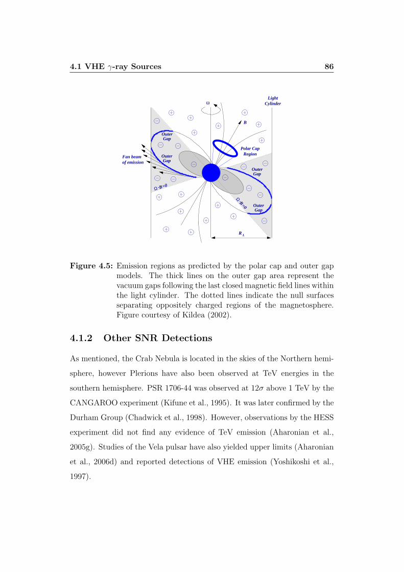
4.1 VHE γ-ray Sources 86

Polar CapRegion

LightCylinder

of emissionFan beam

B=0Ω .

OuterGap

OuterGap

OuterGap

OuterGap

ω

R L

B

B=0

Ω .

Figure 4.5: Emission regions as predicted by the polar cap and outer gapmodels. The thick lines on the outer gap area represent thevacuum gaps following the last closed magnetic field lines withinthe light cylinder. The dotted lines indicate the null surfacesseparating oppositely charged regions of the magnetosphere.Figure courtesy of Kildea (2002).

4.1.2 Other SNR Detections

As mentioned, the Crab Nebula is located in the skies of the Northern hemi-

sphere, however Plerions have also been observed at TeV energies in the

southern hemisphere. PSR 1706-44 was observed at 12σ above 1 TeV by the

CANGAROO experiment (Kifune et al., 1995). It was later confirmed by the

Durham Group (Chadwick et al., 1998). However, observations by the HESS

experiment did not find any evidence of TeV emission (Aharonian et al.,

2005g). Studies of the Vela pulsar have also yielded upper limits (Aharonian

et al., 2006d) and reported detections of VHE emission (Yoshikoshi et al.,

1997).

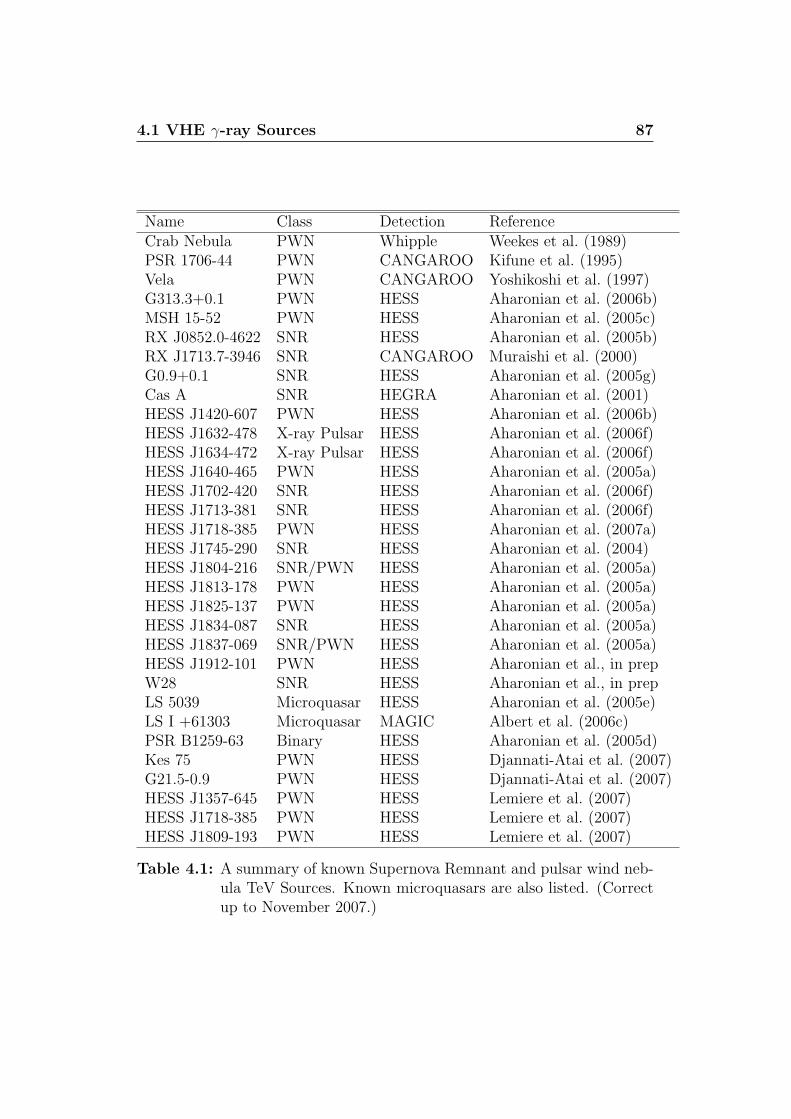
4.1 VHE γ-ray Sources 87

Name Class Detection ReferenceCrab Nebula PWN Whipple Weekes et al. (1989)PSR 1706-44 PWN CANGAROO Kifune et al. (1995)Vela PWN CANGAROO Yoshikoshi et al. (1997)G313.3+0.1 PWN HESS Aharonian et al. (2006b)MSH 15-52 PWN HESS Aharonian et al. (2005c)RX J0852.0-4622 SNR HESS Aharonian et al. (2005b)RX J1713.7-3946 SNR CANGAROO Muraishi et al. (2000)G0.9+0.1 SNR HESS Aharonian et al. (2005g)Cas A SNR HEGRA Aharonian et al. (2001)HESS J1420-607 PWN HESS Aharonian et al. (2006b)HESS J1632-478 X-ray Pulsar HESS Aharonian et al. (2006f)HESS J1634-472 X-ray Pulsar HESS Aharonian et al. (2006f)HESS J1640-465 PWN HESS Aharonian et al. (2005a)HESS J1702-420 SNR HESS Aharonian et al. (2006f)HESS J1713-381 SNR HESS Aharonian et al. (2006f)HESS J1718-385 PWN HESS Aharonian et al. (2007a)HESS J1745-290 SNR HESS Aharonian et al. (2004)HESS J1804-216 SNR/PWN HESS Aharonian et al. (2005a)HESS J1813-178 PWN HESS Aharonian et al. (2005a)HESS J1825-137 PWN HESS Aharonian et al. (2005a)HESS J1834-087 SNR HESS Aharonian et al. (2005a)HESS J1837-069 SNR/PWN HESS Aharonian et al. (2005a)HESS J1912-101 PWN HESS Aharonian et al., in prepW28 SNR HESS Aharonian et al., in prepLS 5039 Microquasar HESS Aharonian et al. (2005e)LS I +61303 Microquasar MAGIC Albert et al. (2006c)PSR B1259-63 Binary HESS Aharonian et al. (2005d)Kes 75 PWN HESS Djannati-Atai et al. (2007)G21.5-0.9 PWN HESS Djannati-Atai et al. (2007)HESS J1357-645 PWN HESS Lemiere et al. (2007)HESS J1718-385 PWN HESS Lemiere et al. (2007)HESS J1809-193 PWN HESS Lemiere et al. (2007)

Table 4.1: A summary of known Supernova Remnant and pulsar wind neb-ula TeV Sources. Known microquasars are also listed. (Correctup to November 2007.)

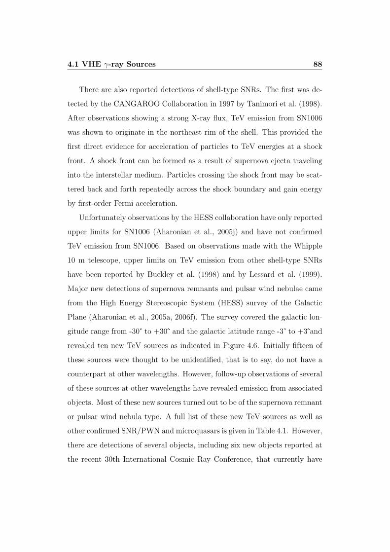
4.1 VHE γ-ray Sources 88

There are also reported detections of shell-type SNRs. The first was de-

tected by the CANGAROO Collaboration in 1997 by Tanimori et al. (1998).

After observations showing a strong X-ray flux, TeV emission from SN1006

was shown to originate in the northeast rim of the shell. This provided the

first direct evidence for acceleration of particles to TeV energies at a shock

front. A shock front can be formed as a result of supernova ejecta traveling

into the interstellar medium. Particles crossing the shock front may be scat-

tered back and forth repeatedly across the shock boundary and gain energy

by first-order Fermi acceleration.

Unfortunately observations by the HESS collaboration have only reported

upper limits for SN1006 (Aharonian et al., 2005j) and have not confirmed

TeV emission from SN1006. Based on observations made with the Whipple

10 m telescope, upper limits on TeV emission from other shell-type SNRs

have been reported by Buckley et al. (1998) and by Lessard et al. (1999).

Major new detections of supernova remnants and pulsar wind nebulae came

from the High Energy Stereoscopic System (HESS) survey of the Galactic

Plane (Aharonian et al., 2005a, 2006f). The survey covered the galactic lon-

gitude range from -30° to +30° and the galactic latitude range -3° to +3°and

revealed ten new TeV sources as indicated in Figure 4.6. Initially fifteen of

these sources were thought to be unidentified, that is to say, do not have a

counterpart at other wavelengths. However, follow-up observations of several

of these sources at other wavelengths have revealed emission from associated

objects. Most of these new sources turned out to be of the supernova remnant

or pulsar wind nebula type. A full list of these new TeV sources as well as

other confirmed SNR/PWN and microquasars is given in Table 4.1. However,

there are detections of several objects, including six new objects reported at

the recent 30th International Cosmic Ray Conference, that currently have

4.1 VHE γ-ray Sources 89

Figure 4.6: A sky map indicating the extent of the 2004 HESS survey of thegalactic plane. The colours represent the range in significancevalues detected in the different regions of the Milky Way galac-tic plane. The extent of the survey was from galactic longitude-30° to +30° and latitude -3° to +3°. Figure from Aharonianet al. (2005a).

4.1 VHE γ-ray Sources 90

no counterparts at other wavelengths.

4.1.3 Unidentified sources

During its operational lifetime, the EGRET (Energetic Gamma-Ray Experi-

ment Telescope) aboard NASA’s Compton Gamma-Ray Observatory (CGRO)

detected over 200 unidentified sources of γ-ray emission. This accounts for

approximately two thirds of the total number of sources seen by this instru-

ment. As these objects have not been identified with any known astrophysical

objects, their origin remains a mystery. The poor angular resolution of the

EGRET instrument is more than likely the reason these objects are uniden-

tified. However, it is possible that some of these objects do constitute a new

class of astrophysical object that emit only in γ-rays and are also referred

to as dark accelerators. A major key to the identification of many of these

unidentified sources will be the successor to EGRET, GLAST (Gamma-ray

Large Area Space Telescope), and new low-energy threshold ground-based

detectors.

With regard to unidentified sources detected at TeV energies, the first

discovery was TeV J2032+4130. This object was discovered serendipitously

by the Crimean Astrophysical Observatory during observations of Cygnus X-

3 (Neshpor et al., 1995). During independent observations of the Cygnus X-3

region, the High Energy Gamma Ray Astronomy (HEGRA) group detected

TeV J2032+4130 while observing a separate object (Aharonian et al., 2002).

TeV J2032+4130 currently has no known counterpart at other wavelengths.

It has been suggested that the VHE γ-ray emission from TeV J2032+4130

may be associated with the strong OB stellar association of the Cygnus re-

gion (Aharonian et al., 2002). It is possible that the stellar winds of the hot

young stars in the OB association of Cygnus OB2 are the source of the accel-

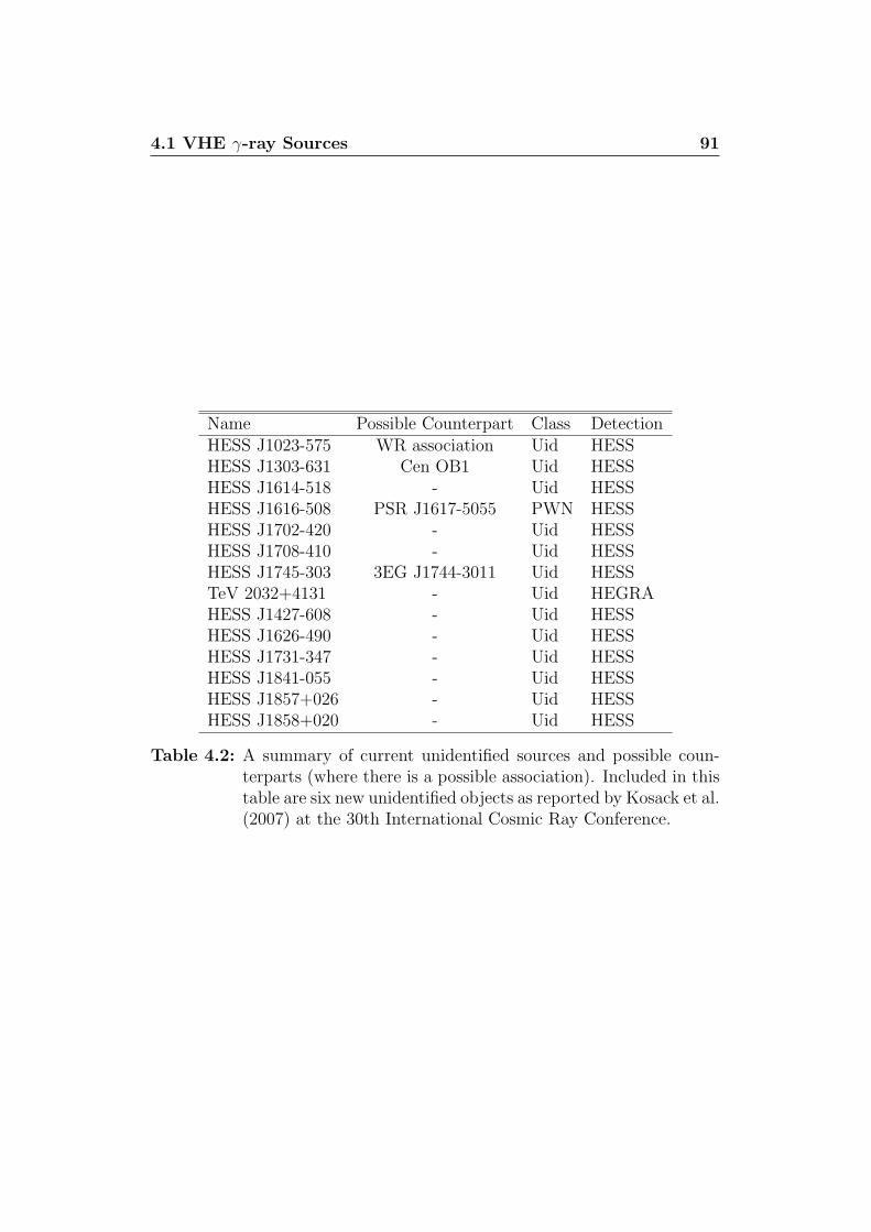
4.1 VHE γ-ray Sources 91

Name Possible Counterpart Class DetectionHESS J1023-575 WR association Uid HESSHESS J1303-631 Cen OB1 Uid HESSHESS J1614-518 - Uid HESSHESS J1616-508 PSR J1617-5055 PWN HESSHESS J1702-420 - Uid HESSHESS J1708-410 - Uid HESSHESS J1745-303 3EG J1744-3011 Uid HESSTeV 2032+4131 - Uid HEGRAHESS J1427-608 - Uid HESSHESS J1626-490 - Uid HESSHESS J1731-347 - Uid HESSHESS J1841-055 - Uid HESSHESS J1857+026 - Uid HESSHESS J1858+020 - Uid HESS

Table 4.2: A summary of current unidentified sources and possible coun-terparts (where there is a possible association). Included in thistable are six new unidentified objects as reported by Kosack et al.(2007) at the 30th International Cosmic Ray Conference.

4.1 VHE γ-ray Sources 92

erating component of the hadrons of the cosmic radiation that results in the

production of γ-rays. HESS J1616-508, a recently reported dark accelerator,

is similar to TeV J2032+4130 in that it lies in a region of sky containing sev-

eral other astrophysical objects of interest. However, it is likely that HESS

J1616-508 is powered by the pulsar wind nebula PSR J1617-5055. Figure 4.7

shows a sky map containing the source HESS J1616-508.

Figure 4.7: A TEV sky map illustrating the crowded region of sky contain-ing the source HESS J1616-508 taken from Aharonian et al.(2006f).

Another source was discovered by HESS in the same manner as TeV

J2032+4130. During observations of the binary pulsar PSR B1259-63, the

4.1 VHE γ-ray Sources 93

new object, HESS J1303-631, was detected in the same field of view (Aharo-

nian et al., 2005h; Beilicke et al., 2005b,a). HESS J1303-631 was discovered

approximately 0.6° north of PSR B1259-63 and, like TeV J2032+4130, is

close to an association of OB stars, namely Cen OB 1 (Hartkopf et al., 1999;

Aharonian et al., 2005h). More observations, including multi-wavelength

observations, of these sources are required to try and clarify their origin,

as happened in the case of many of the initial unidentified sources. Multi-

wavelength observations will help confirm or reject, the possible counterparts

associated with some of the objects. Table 4.2 lists the current catalogue of

unidentified VHE sources. Note here that a possible counterpart is given in

some cases. If a counterpart is not confirmed, it is possible that the uniden-

tified sources mentioned above represent a new form of previously unknown

dark TeV γ-ray emitter or “dark accelerator”. Very recently, during the 30th

International Cosmic Ray Conference, the HESS collaboration announced

the detection of a further six unidentified VHE γ-ray sources (Kosack et al.,

2007).

4.1.4 Dark Accelerators

The term dark accelerator has come to be associated with VHE sources that

appear to have no detectable signal at other wavelengths. Dark accelerators

are the newest classification designated to some of the most recent and as

yet unidentified sources of VHE γ-rays. These sources tend to have low

galactic latitudes, with only a few arcmin of angular size, and hence they

are believed to be galactic in origin. As mentioned, they appear to have no

known counterparts at other wavelengths and may show variability in TeV

γ-rays. There have been several proposals suggested for the origin of VHE

photons from these objects. The main production models regarding dark

4.1 VHE γ-ray Sources 94

accelerators are discussed in Chapter 7 along with a discussion on the results

of the analysis performed on TeV J2032+4130 as part of this project.

4.1.5 Other Sources of TeV γ-rays

There are many other important sources of VHE γ-rays in the universe, some

of which are briefly mentioned here.

Active Galactic Nuclei

Active Galactic Nuclei (AGN) is the collective term used to refer to quasars,

blazars, Seyfert galaxies, and radio galaxies. AGN are the most powerful

sources of luminosity in the universe. The activities of these galaxies comes

from an energy source located at its centre. A characteristic of AGN is the

observed variability of their brightness. In fact emission from AGN can be

variable on time scales of months to years and in some cases the variability

can have time scales of days and hours. The variability of VHE γ-ray emis-

sion provides information regarding the size of the object emitting the radi-

ation and leads to the conclusion that the immense energy emanating from

AGN comes from a relatively small volume. The central sources of energy

of AGN are thought to be powered by supermassive black holes which draw

surrounding matter into a rotating accretion disk. The accreted matter then

loses angular momentum through turbulent forces. Thermal emission from

the accretion disk peaks at UV/X-ray wavelengths. Beyond the accretion

disk lies a region, commonly regarded as torus shaped, which absorbs visible

and UV light along some lines of sight. Along the axis of rotation of the

accretion disk, jets of energetic particles stream perpendicularly away from

the plane of the host galaxy.

These jets of relativistic particles and plasma outflows are thought to be

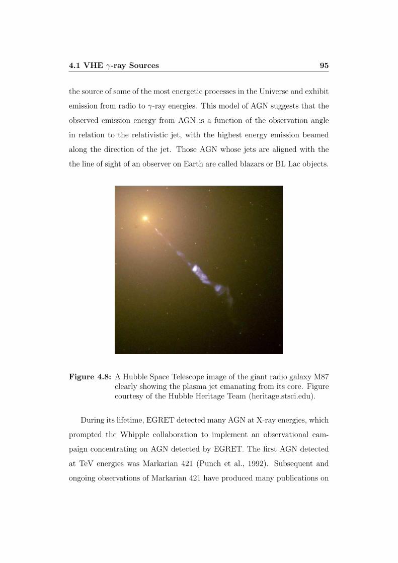
4.1 VHE γ-ray Sources 95

the source of some of the most energetic processes in the Universe and exhibit

emission from radio to γ-ray energies. This model of AGN suggests that the

observed emission energy from AGN is a function of the observation angle

in relation to the relativistic jet, with the highest energy emission beamed

along the direction of the jet. Those AGN whose jets are aligned with the

the line of sight of an observer on Earth are called blazars or BL Lac objects.

Figure 4.8: A Hubble Space Telescope image of the giant radio galaxy M87clearly showing the plasma jet emanating from its core. Figurecourtesy of the Hubble Heritage Team (heritage.stsci.edu).

During its lifetime, EGRET detected many AGN at X-ray energies, which

prompted the Whipple collaboration to implement an observational cam-

paign concentrating on AGN detected by EGRET. The first AGN detected

at TeV energies was Markarian 421 (Punch et al., 1992). Subsequent and

ongoing observations of Markarian 421 have produced many publications on

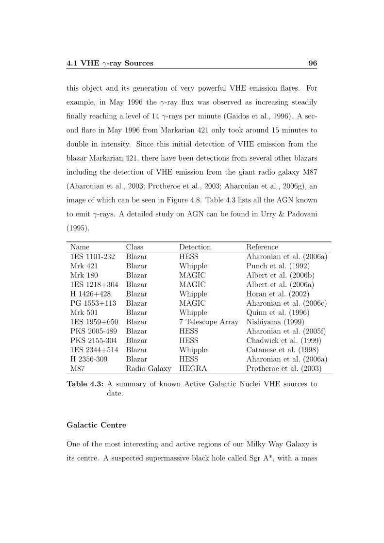
4.1 VHE γ-ray Sources 96

this object and its generation of very powerful VHE emission flares. For

example, in May 1996 the γ-ray flux was observed as increasing steadily

finally reaching a level of 14 γ-rays per minute (Gaidos et al., 1996). A sec-

ond flare in May 1996 from Markarian 421 only took around 15 minutes to

double in intensity. Since this initial detection of VHE emission from the

blazar Markarian 421, there have been detections from several other blazars

including the detection of VHE emission from the giant radio galaxy M87

(Aharonian et al., 2003; Protheroe et al., 2003; Aharonian et al., 2006g), an

image of which can be seen in Figure 4.8. Table 4.3 lists all the AGN known

to emit γ-rays. A detailed study on AGN can be found in Urry & Padovani

(1995).

Name Class Detection Reference1ES 1101-232 Blazar HESS Aharonian et al. (2006a)Mrk 421 Blazar Whipple Punch et al. (1992)Mrk 180 Blazar MAGIC Albert et al. (2006b)1ES 1218+304 Blazar MAGIC Albert et al. (2006a)H 1426+428 Blazar Whipple Horan et al. (2002)PG 1553+113 Blazar MAGIC Aharonian et al. (2006c)Mrk 501 Blazar Whipple Quinn et al. (1996)1ES 1959+650 Blazar 7 Telescope Array Nishiyama (1999)PKS 2005-489 Blazar HESS Aharonian et al. (2005f)PKS 2155-304 Blazar HESS Chadwick et al. (1999)1ES 2344+514 Blazar Whipple Catanese et al. (1998)H 2356-309 Blazar HESS Aharonian et al. (2006a)M87 Radio Galaxy HEGRA Protheroe et al. (2003)

Table 4.3: A summary of known Active Galactic Nuclei VHE sources todate.

Galactic Centre

One of the most interesting and active regions of our Milky Way Galaxy is

its centre. A suspected supermassive black hole called Sgr A*, with a mass

4.2 Major Imaging Atmospheric Cherenkov Experiments 97

of 2.6 × 106 M¯, is believed to be located at the galactic centre (Genzel &

Townes, 1987; Schodel et al., 2002; Atoyan & Dermer, 2004). The Chandra

X-ray Observatory recently revealed the presence of several compact objects

surrounding the black hole (Baganoff et al., 2003). The X-ray variability of

these objects suggests that they can be identified as neutron stars or black

holes. The galactic centre was detected by the Whipple 10 m telescope in

2004 (Kosack et al., 2004) and by two other experiments that year (Aharonian

et al., 2004; Tsuchiya, 2004). The HESS collaboration have recently reported

the detection of γ-ray emission from the source HESS J1745-290 located 0.1°from the galactic centre (Aharonian et al., 2006e). However, as there is a high

density of candidate objects emitting non-thermal radiation from within the

source region, the nature of the emission from HESS J1745-290 is at present

unclear.

4.2 Major Imaging Atmospheric Cherenkov

Experiments

Ground-based γ-ray detectors are unique in astronomy as they do not in-

teract directly with the primary photon. Imaging atmospheric Cherenkov

telescopes detect the extensive air shower induced by the primary particle

(with energy between 100 GeV and 50 TeV), after it collides with nuclei

in the Earth’s atmosphere. Since the first theoretical prediction (Morrison,

1958), the practical techniques of ground-based γ-ray detection have had to

deal with several natural limits:

Since the Earth’s atmosphere is opaque to VHE photons, even at moun-

tain altitudes, the primary photon will interact electromagnetically

with the nuclei in the atmosphere. The thicker the atmosphere the

4.2 Major Imaging Atmospheric Cherenkov Experiments 98

more interaction there will be and hence the energy of the primary

will be dissipated more rapidly. Due to this atmospheric absorption

it is necessary to locate γ-ray detectors either above the atmosphere

onboard satellites or balloons, or to use indirect methods to detect

γ-rays from the ground.

The flux of VHE γ-rays from astrophysical sources is low and decreases

rapidly with increasing energy.

At very high energies the cosmic ray flux is much higher than the γ-ray

flux. Hence the need for cosmic ray rejection techniques is essential in

VHE γ-ray astronomy.

There have been several innovative experiments developed since the 1960s

that have attempted to address these problems. These experiments have

evolved into several international collaborations, in both the northern and

southern hemispheres, that have led to many major discoveries in this young

area of astronomy. Imaging atmospheric Cherenkov telescopes have become

the most sensitive instruments used for the detection of VHE γ-rays. The four

main experiments that are either in development, or are currently making

valuable contributions to VHE astronomy, are described below.

4.2.1 HESS

Located in Namibia, the HESS Collaboration operates the major imaging

atmospheric Cherenkov experiment in the southern hemisphere. It has been

in operation as Phase-I since 2003, and is the leader in the field of ground-

based γ-ray astronomy. The HESS array is comprised of four 12 m telescopes

arranged in a square configuration with each side 120 m. Each reflector

is based on the Davies-Cotton design (Hermann, 1997) with a focal plane

4.2 Major Imaging Atmospheric Cherenkov Experiments 99

camera consisting of 960 pixels. The array was completed in 2003 and the

HESS Collaboration has reported many new discoveries of VHE γ-ray sources

since it was comissioned. To date the HESS catalogue contains 35 sources.

Several of these objects were discovered in the central part of our galaxy, two

of which are reported as dark accelerators (Aharonian et al., 2005a). The

HESS collaboration has also reported a detection of the Crab Nebula at 21σ

in 4.7 hours (Hinton, 2004). In Phase-II of HESS, it is planned to add a fifth

large diameter telescope at the centre of the current array, increasing the

angular resolution, energy range, and sensitivity of the instrument further.

4.2.2 The VERITAS Collaboration

The VERITAS (Very Energetic Radiation Imaging Telescope Array System)

Collaboration is the successor to what was known as the Whipple Collabora-

tion. It is led by the Smithsonian Astrophysical Observatory and currently

consists of scientists from academic institutions in the United States of Amer-

ica, the United Kingdom, Canada and Ireland. The main objective of the

group is the search for, and study of, galactic and extra-galactic sources of

Very High Energy γ-rays. The collaboration operates and maintains a 10

m imaging atmospheric Cherenkov telescope at the Fred Lawrence Whipple

Observatory on Mount Hopkins, in Southern Arizona. The Whipple 10 m

imaging atmospheric Cherenkov telescope was the first ground-based instru-

ment that successfully used the Cherenkov Imaging Technique to detect VHE

γ-rays at ground level (Weekes et al., 1989).

The current generation of imaging atmospheric Cherenkov experiments

consists of arrays of several reflectors and the VERITAS Collaboration is

now operating an array of four twelve-metre reflectors (Kieda, 2007; Weekes,

2007). Results from early observations were reported at the 30th Interna-

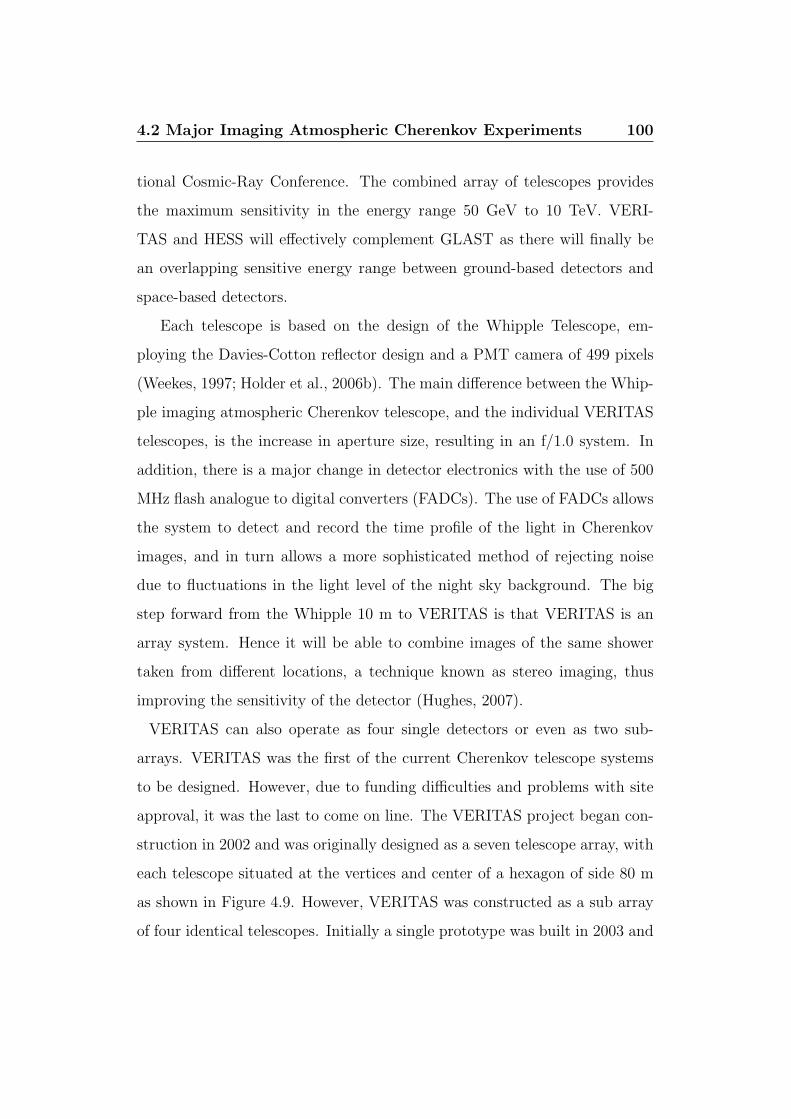
4.2 Major Imaging Atmospheric Cherenkov Experiments 100

tional Cosmic-Ray Conference. The combined array of telescopes provides

the maximum sensitivity in the energy range 50 GeV to 10 TeV. VERI-

TAS and HESS will effectively complement GLAST as there will finally be

an overlapping sensitive energy range between ground-based detectors and

space-based detectors.

Each telescope is based on the design of the Whipple Telescope, em-

ploying the Davies-Cotton reflector design and a PMT camera of 499 pixels

(Weekes, 1997; Holder et al., 2006b). The main difference between the Whip-

ple imaging atmospheric Cherenkov telescope, and the individual VERITAS

telescopes, is the increase in aperture size, resulting in an f/1.0 system. In

addition, there is a major change in detector electronics with the use of 500

MHz flash analogue to digital converters (FADCs). The use of FADCs allows

the system to detect and record the time profile of the light in Cherenkov

images, and in turn allows a more sophisticated method of rejecting noise

due to fluctuations in the light level of the night sky background. The big

step forward from the Whipple 10 m to VERITAS is that VERITAS is an

array system. Hence it will be able to combine images of the same shower

taken from different locations, a technique known as stereo imaging, thus

improving the sensitivity of the detector (Hughes, 2007).

VERITAS can also operate as four single detectors or even as two sub-

arrays. VERITAS was the first of the current Cherenkov telescope systems

to be designed. However, due to funding difficulties and problems with site

approval, it was the last to come on line. The VERITAS project began con-

struction in 2002 and was originally designed as a seven telescope array, with

each telescope situated at the vertices and center of a hexagon of side 80 m

as shown in Figure 4.9. However, VERITAS was constructed as a sub array

of four identical telescopes. Initially a single prototype was built in 2003 and

4.2 Major Imaging Atmospheric Cherenkov Experiments 101

Figure 4.9: A schematic of the original seven telescope VERITAS array.The locations of the telescopes of the VERITAS-4 sub arrayare also shown.

operated in engineering mode for several months in order to test and develop

custom-made hardware and software (Holder et al., 2006a). The second stage

of development saw the construction of three more identical telescopes at the

base camp of the Fred Lawrence Whipple Observatory. VERITAS is expected

to substantially increase the catalogue of very high energy γ-ray sources in

the northern hemisphere and greatly improve measurements of established

sources. Holder et al. (2006b) provides a current report of the VERITAS

project. In addition to the new array system, the VERITAS Collaboration

continues to operate the Whipple 10 m telescope for deep observations of

AGN and supernova targets.

4.2.3 MAGIC

The MAGIC Collaboration is composed of research institutions from Italy,

Germany and Spain, with the telescope located at an altitude of 2200 m

4.2 Major Imaging Atmospheric Cherenkov Experiments 102

in La Palma, Spain (Cortina et al., 2005). MAGIC differs from the other

current imaging atmospheric Cherenkov instruments in that it is comprised

of only one reflector. The reflector is 17 m in diameter and is supported by

a light weight carbon-fibre frame. The camera is constructed from advanced

hemispherical PMTs and utilises a 300 MHz flash analog-to-digital-converter

system similar to the VERITAS system. MAGIC has detected the Crab

Nebula at the 16σ level in just over one hour (Wagner et al., 2005) and

detected Mrk 421 at 29σ in 277 minutes (Albert et al., 2007a). MAGIC has

a low-energy threshold between 20 GeV and 30 GeV (Fonseca, 1999; Flix

et al., 2004) and, due to its light weight frame, has a rapid slew time making

it ideal to respond quickly to γ-ray burst alerts. The MAGIC Collaboration

are currently building a second telescope, MAGIC-II (Baixeras et al., 2005),

on the same site on La Palma, at 85m distance from MAGIC while the

collaboration continues to study galactic and extragalactic sources (Albert

et al., 2007b).

4.2.4 CANGAROO-III

CANGAROO-III is a second imaging atmospheric Cherenkov telescope col-

laboration located in the southern hemisphere (Enomoto et al., 2002, 2006).

It is operated by the Australian-Japanese CANGAROO group. Originally

it was an array-type system with four telescopes arranged in a square. The

spacing between the sides of the square array of telescopes is 100 m. However,

one of the telescopes has since been retired and the array is now comprised

of three telescopes. CANGAROO differs from HESS and VERITAS in that

a parabolic mirror is used in the optical design. The focal plane camera is

composed of 427 pixels.

4.3 The Milagro Detector 103

4.3 The Milagro Detector

The previous sections detail the main experiments that use the imaging at-

mospheric Cherenkov technique. However, Milagro is an experiment based

on a different detection technique that has a relevance to the detection of

unidentified sources of VHE γ-rays. The Milagro γ-ray detector (Smith,

2005) is located in the Jemez Mountains of northern New Mexico (35.9.° N,

106.7. ° W) at an altitude of 2630 m above sea level. It is a water Cherenkov

air-shower detector and is comprised of a 5000 m2 pond surrounded by 175

outrigger tanks totaling an area of 40 000 m2. The main tank contains 6

million gallons of water and has two layers of PMTs. The first layer is used

to detect the Cherenkov light from the relativistic particles produced by the

interaction of γ-rays and particles in the atmosphere and is placed under

4 radiation lengths of water. The second layer of PMTs is used to help in

background rejection of cosmic rays which tend to have a more penetrating

component. This second layer of PMTs is placed under 16 radiation lengths

of water. The overall system results in Milagro having an energy threshold

of around 250 GeV. However, compared to imaging atmospheric Cherenkov

telescopes, Milagro has a higher energy threshold with the median energy of

detected events about 20 TeV. It also has a reduced angular resolution of

about 1°.A major advantage of this kind of detector over Cherenkov telescopes

is the fact that they can operate continuously with the result that a large

portion of the sky can be monitored. Milagro detected the Crab Nebula

and the AGN Mrk 421 during a galactic plane survey (Atkins et al., 2004).

The Milagro experiment recently reported the detection of two objects, C1

and C2, in the Cygnus region of the sky with no known counterparts at

other wavelengths (Abdo et al., 2007). Also reported was the detection of a

4.4 Summary 104

source consistent with the reported location of TeV J2032+4130. The source

MGRO J2031+41 was observed in an area with the largest concentration of

molecular and atomic gas in the Cygnus region. The authors also reported

that the spatial extent of MGRO J2031+41 is much larger than the extent

of TeV J2032+4130 and leads to the conclusion that there is another source,

or sources, contributing to the Milagro detection.

4.4 Summary

Apart from the main collaborations described above, there are also other

imaging atmospheric Cherenkov telescopes operational today. These include

CACTUS, PACT, STACEE, TACTIC and Whipple. A full list of the main

operational imaging atmospheric Cherenkov telescope experiments is shown

in Table 4.4. CACTUS, PACT and STACEE are wavefront sampling tele-

scopes that detect the Cherenkov radiation at many different locations on

the ground using large mirror arrays. With this wide range of instruments,

with improved sensitivities and lower thresholds, now devoted to VHE γ-

ray astronomy, it is expected that many more sources of VHE γ-ray emission

will be detected over the course of their lifetime and will thus expand the

catalogue of VHE sources further. As the experiments are located in both

the northern and southern hemispheres, a complete map of the very high

energy universe can finally be constructed. When the next generation of

space-based detectors are operational their energy ranges will overlap those

of the new ground-based experiments. This will result in a crucial gap in the

electromagnetic spectrum finally being accessible for study. Coverage of the

VHE spectrum will also be improved by the next generation of ground-based

telescopes (e.g. MAGIC II and HESS II).

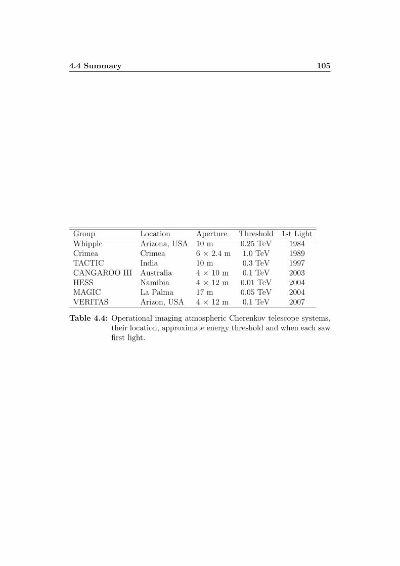
4.4 Summary 105

Group Location Aperture Threshold 1st LightWhipple Arizona, USA 10 m 0.25 TeV 1984Crimea Crimea 6 × 2.4 m 1.0 TeV 1989TACTIC India 10 m 0.3 TeV 1997CANGAROO III Australia 4 × 10 m 0.1 TeV 2003HESS Namibia 4 × 12 m 0.01 TeV 2004MAGIC La Palma 17 m 0.05 TeV 2004VERITAS Arizon, USA 4 × 12 m 0.1 TeV 2007

Table 4.4: Operational imaging atmospheric Cherenkov telescope systems,their location, approximate energy threshold and when each sawfirst light.

Chapter 5

VERITAS Reflector Alignment

and Point Spread Function.

5.1 Introduction

The previous chapter detailed the Imaging Atmospheric Cherenkov Tech-

nique and its associated instrumentation. At the outset of this project, VER-

ITAS, the current generation of atmospheric Cherenkov telescopes located in

the Northern Hemisphere, was beginning to come on-line. The VERITAS

Collaboration has recently completed and are currently operating a four-

telescope array system in Southern Arizona as the successor to the Whipple

10 m atmospheric Cherenkov telescope (Figure 5.1).

The four VERITAS telescopes are based on the Whipple 10 m design.

Each telescope has an aperture of 12 m and focal length of 12 m, resulting in

an f/1 system, thus reducing the optical aberrations of the telescope. Each

telescope has a 499 pixel camera with a field of view of 3.5° and consists

of ∼ 350 mirror facets. It is anticipated that an energy threshold of ∼ 100

GeV will be achieved when all four telescopes have been fully optimised and

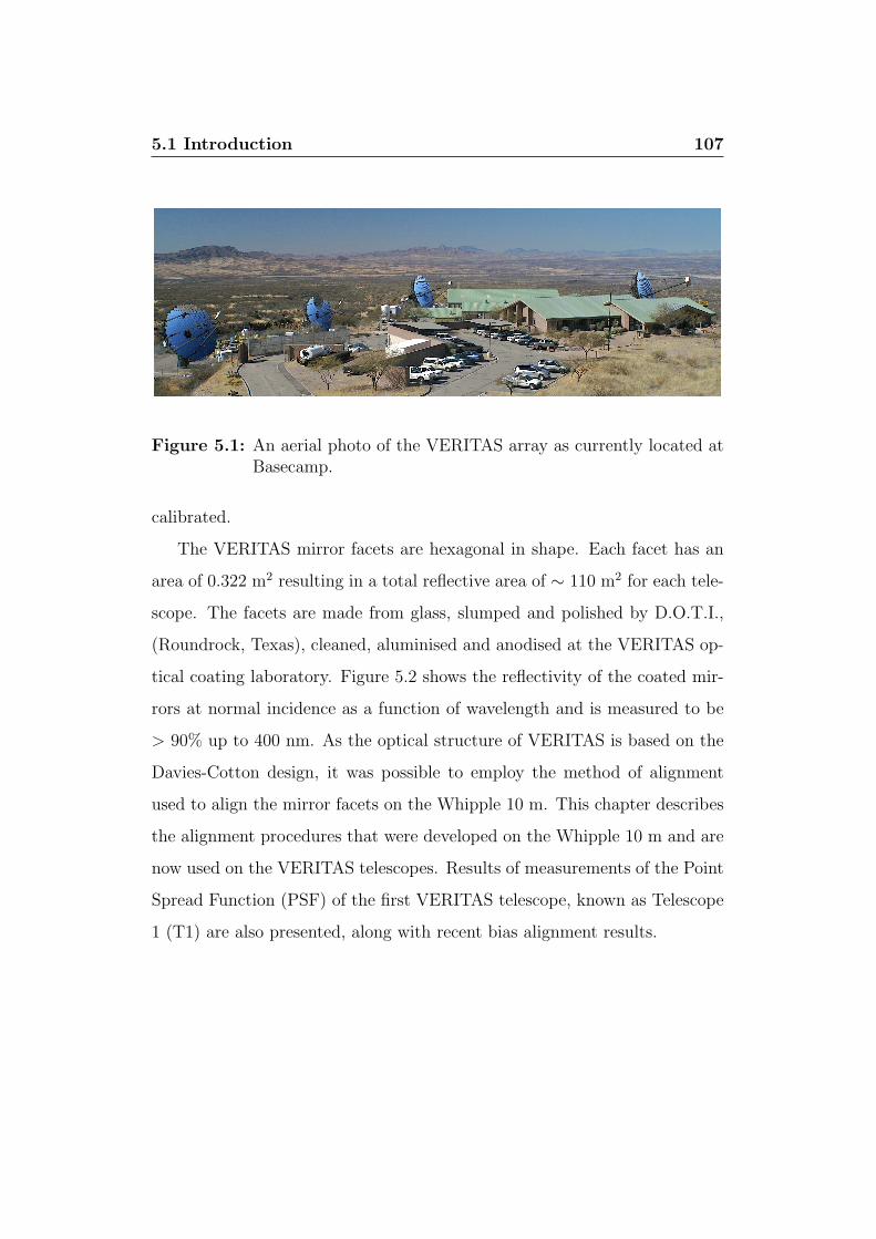
5.1 Introduction 107

Figure 5.1: An aerial photo of the VERITAS array as currently located atBasecamp.

calibrated.

The VERITAS mirror facets are hexagonal in shape. Each facet has an

area of 0.322 m2 resulting in a total reflective area of ∼ 110 m2 for each tele-

scope. The facets are made from glass, slumped and polished by D.O.T.I.,

(Roundrock, Texas), cleaned, aluminised and anodised at the VERITAS op-

tical coating laboratory. Figure 5.2 shows the reflectivity of the coated mir-

rors at normal incidence as a function of wavelength and is measured to be

> 90% up to 400 nm. As the optical structure of VERITAS is based on the

Davies-Cotton design, it was possible to employ the method of alignment

used to align the mirror facets on the Whipple 10 m. This chapter describes

the alignment procedures that were developed on the Whipple 10 m and are

now used on the VERITAS telescopes. Results of measurements of the Point

Spread Function (PSF) of the first VERITAS telescope, known as Telescope

1 (T1) are also presented, along with recent bias alignment results.

5.1 Introduction 108

Figure 5.2: Mirror reflectivity as a function of wavelength for light normallyincident to the mirror surface.

5.2 Point Spread Function 109

5.2 Point Spread Function

All optical systems suffer to some extent from aberrations. The image of a

point source such as a star acts as a good measure of the degree of degradation

caused by aberrations. When an optical system images a point source, the

image of this source will not be a point. The optical system will introduce a

certain amount of blur in the resulting image and thus distorts our view of

the object being observed. This degradation can be represented by means of

a Point Spread Function (PSF).

Mirror alignment is performed on the mirror facets of the VERITAS tele-

scopes (and the Whipple 10 m) with the aim of producing as small a PSF

as possible. However the PSF will always have some intrinsic width due to

optical aberrations that are associated with the Davies-Cotton reflector de-

sign. For on-axis images the main aberrations are spherical, coma and most

significantly astigmatism. With off-axis images coma becomes the dominant

aberration (Lewis, 1990). PSF measurement involves the imaging of a bright

star on the focal plane of the camera. A CCD camera mounted in the centre

of the reflector is used to record the optical image of the star that is seen

on a target screen covering the PMT camera. Star images are captured at

several elevations and the Full Width at Half Maximum (FWHM) of the PSF

is then calculated using the skycat image processing programme and is used

as a measure of the degree of alignment of the facets.

The PSF’s of the VERITAS reflectors are measured regularly throughout

the observing season to look for signs of misalignment of the mirror facets.

Depending on the amount of degradation, a realignment of some or all of the

mirror facets may be required. Following PSF measurements of the Whipple

10 m taken during 2001/2002 observing season it was noted that the FWHM

of the PSF grew significantly with increasing elevation Kildea (2002). The

5.2 Point Spread Function 110

Facet Tilt When Telescope Moves From0° to 30° Elevation

x = no measurement

Scale

0.1°

x

x x

x x x

x x x

x

x

Figure 5.3: Vector plot representation of the size and direction of the move-ment of the mirror facets of the Whipple 10 m when the tele-scope pointing is changed in elevation from 0° to 30°. Figurecourtesy of Schroedter (2004).

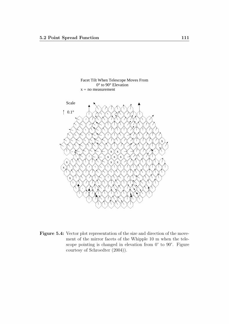
5.2 Point Spread Function 111

Facet Tilt When Telescope Moves From0° to 90° Elevation

x = no measurement

Scale

0.1°

x

x x

x x x

x x x

x

x

Figure 5.4: Vector plot representation of the size and direction of the move-ment of the mirror facets of the Whipple 10 m when the tele-scope pointing is changed in elevation from 0° to 90°. Figurecourtesy of Schroedter (2004)).

5.3 Optical Alignment 112

conclusions drawn from these measurements suggested that when the optical

support structure, quadrapod arms, and PMT camera increased in elevation

the change in the weight distribution caused the mirrors to change position

slightly.

Since the optical support structure is not completely rigid, the steel struc-

ture will bend and twist in a complex way due to the relative change of di-

rection of the force of gravity on each section of the optical support structure

as the telescope’s elevation changes. Since the mirrors are attached to the

optical support structure via a triangular mount, which itself is connected to

two separate optical support structure beams, it is reasonable to assume that

they will move slightly due to sagging of the optical support structure and

hence get misaligned at higher elevations. Figures 5.3 and 5.4 show vectors

on each facet representing the measured size and direction of the movement

(relative to the optical support structure) of the mirrors with increasing el-

evation. In an effort to reverse this misalignment a bias alignment method

was derived to improve the optical qualities of the Whipple reflector.

5.3 Optical Alignment

For the Davies-Cotton reflector design to be used as an effective light collec-

tor, each of its individual mirror elements must be correctly aligned. Every

facet is required to reflect an incoming beam of light that is parallel to the

optic axis to a point in the center of the focal plane. A beam of light whose

incoming angle is offset slightly with respect to the optic axis will be dis-

placed in proportion to the plate-scale factor (Section 3.1.1). To facilitate

alignment, each facet is attached to the optical support structure using three

adjustable bolts, arranged at the corners of a triangular mount (Figure 5.5).

5.3 Optical Alignment 113

When correctly aligned, the normal vector at the centre of each facet will be

Figure 5.5: A picture of an individual mirror facet mount clearly showingthe mounting bolts for the mirror facets.

aligned to a point on the optic axis twice the focal length1 of the telescope,

away from the centre of the telescope, and the instrument will form an image

at the focal plane. Figure 5.6 illustrates why this is the case; the centre of

the facet (A), the centre of the image plane (B), and the 2f point on the optic

axis (C ), form an isosceles triangle since the angles x, y & z are equal. The

alignment procedure consists of placing a laser at the 2f point, or alignment

point, on the optic axis and adjusting the pointing of each of the 350 facets

so that they retro-reflect as shown in Figure 5.6.

1Twice the focal length is 24 m for the VERITAS telescopes and 14.6 m for the Whipple10 m telescope.

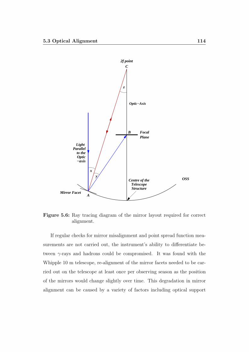
5.3 Optical Alignment 114

z

x

yCentre of the

TelescopeStructure

2f point

Light Parallel

to theOptic−axis

B

C

OSS

A

Optic−Axis

Mirror Facet

FocalPlane

Figure 5.6: Ray tracing diagram of the mirror layout required for correctalignment.

If regular checks for mirror misalignment and point spread function mea-

surements are not carried out, the instrument’s ability to differentiate be-

tween γ-rays and hadrons could be compromised. It was found with the

Whipple 10 m telescope, re-alignment of the mirror facets needed to be car-

ried out on the telescope at least once per observing season as the position

of the mirrors would change slightly over time. This degradation in mirror

alignment can be caused by a variety of factors including optical support

5.3 Optical Alignment 115

structure flexure, mirror mount stability, and on rare occasions, due to ex-

treme weather conditions at the Mount Hopkins site. However initial checks

of mirror alignment on T1 suggest that alignment is holding for longer peri-

ods than with the Whipple 10 m telescope. For example it was found that

with the Whipple 10 m telescope, realignment was required at least once

every season, where as with T1, no realignment was required after its initial

alignment.

5.3.1 Manual Alignment Procedure

The manual or standard alignment procedure is undertaken while the tele-

scope is located in the “home” position and was developed as a means to

align the mirror facets of the Whipple 10 m telescope. The home position

has the optic axis of the telescope lying horizontally and pointing towards the

alignment point. The manual alignment system consists of a diverging laser

beam, located at the alignment point, which is directed onto the target facet

via a beam splitter. The beam is spread out to cover as much of the mirror

as possible. This ensures any imperfections in the surface of the mirror are

averaged out. The return beam can then be viewed on a screen (see Figure

5.7).

The telescope must be accurately positioned such that the mechanical

axis is aligned with its 2f point. The operator then manually aims the in-

strument at the target facet and views the reflected image on the screen. If

the mirror is correctly aligned the image will be in the centre of the screen.

Otherwise appropriate instructions are given to a second person located near

the target facet, who then adjusts the mounting bolts until the reflected

image is centered. This process is then repeated for each mirror facet. The

entire procedure can take a crew of ∼ 6 people up to eight hours to complete.

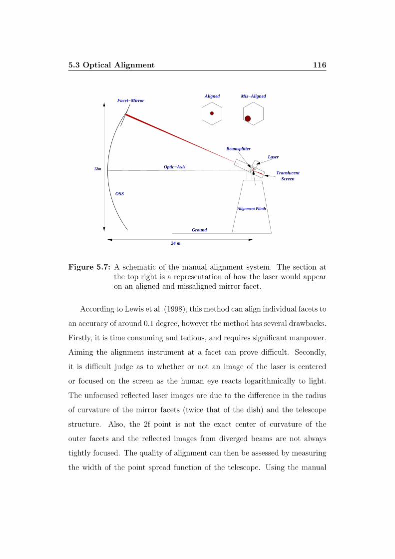
5.3 Optical Alignment 116

TranslucentScreen

OSS

Ground

Laser

Beamsplitter

Mis−AlignedAlignedFacet−Mirror

Optic−Axis

24 m

Alignment Plinth

12m

Figure 5.7: A schematic of the manual alignment system. The section atthe top right is a representation of how the laser would appearon an aligned and missaligned mirror facet.

According to Lewis et al. (1998), this method can align individual facets to

an accuracy of around 0.1 degree, however the method has several drawbacks.

Firstly, it is time consuming and tedious, and requires significant manpower.

Aiming the alignment instrument at a facet can prove difficult. Secondly,

it is difficult judge as to whether or not an image of the laser is centered

or focused on the screen as the human eye reacts logarithmically to light.

The unfocused reflected laser images are due to the difference in the radius

of curvature of the mirror facets (twice that of the dish) and the telescope

structure. Also, the 2f point is not the exact center of curvature of the

outer facets and the reflected images from diverged beams are not always

tightly focused. The quality of alignment can then be assessed by measuring

the width of the point spread function of the telescope. Using the manual

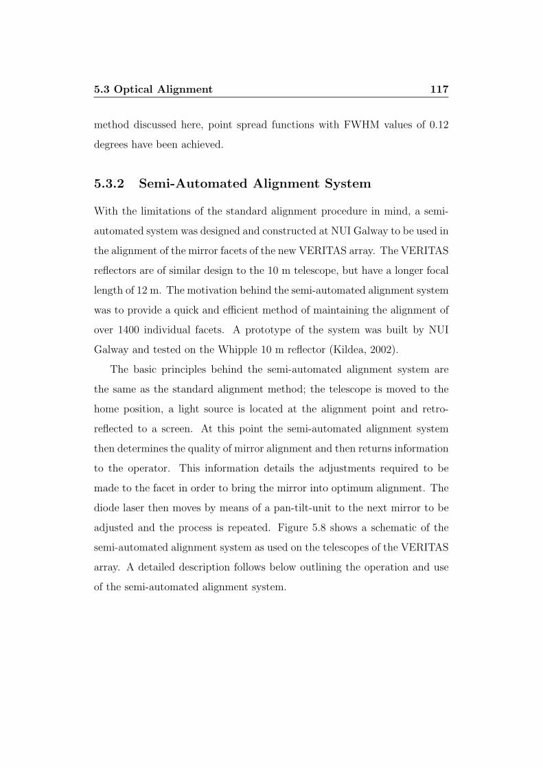
5.3 Optical Alignment 117

method discussed here, point spread functions with FWHM values of 0.12

degrees have been achieved.

5.3.2 Semi-Automated Alignment System

With the limitations of the standard alignment procedure in mind, a semi-

automated system was designed and constructed at NUI Galway to be used in

the alignment of the mirror facets of the new VERITAS array. The VERITAS

reflectors are of similar design to the 10 m telescope, but have a longer focal

length of 12 m. The motivation behind the semi-automated alignment system

was to provide a quick and efficient method of maintaining the alignment of

over 1400 individual facets. A prototype of the system was built by NUI

Galway and tested on the Whipple 10 m reflector (Kildea, 2002).

The basic principles behind the semi-automated alignment system are

the same as the standard alignment method; the telescope is moved to the

home position, a light source is located at the alignment point and retro-

reflected to a screen. At this point the semi-automated alignment system

then determines the quality of mirror alignment and then returns information

to the operator. This information details the adjustments required to be

made to the facet in order to bring the mirror into optimum alignment. The

diode laser then moves by means of a pan-tilt-unit to the next mirror to be

adjusted and the process is repeated. Figure 5.8 shows a schematic of the

semi-automated alignment system as used on the telescopes of the VERITAS

array. A detailed description follows below outlining the operation and use

of the semi-automated alignment system.

5.3 Optical Alignment 118

5.3.3 System description

This system consists of a diode laser and 5 cm cubed double prism beam

splitter mounted on a pan-tilt-unit. The pan-tilt-unit (PTU) is basically

a small motorised alt-azimuth device. It has the provision for mounting a

diode laser to it to enable it to point in a specific direction, i.e. either in

elevation or azimuthal directions. The pan-tilt-unit is mounted (along with

a screen and CCD camera) on a 60 cm x 30 cm optical table as seen in

Figure 5.9. The pan-tilt-unit is a Model 46-70NR from Directed Perceptions

Inc. and the CCD is a model ST-5C from the Santa-Barbara Imaging Group.

Software for both devices was developed at NUI Galway and is written in the

C programming language. A dedicated laptop computer operating under the

Red Hat 9 Linux operating system accompanies the alignment system. The

software controls the pan and tilt angles of the pan-tilt-unit to point the laser

beam in any required direction and, when instructed, the CCD camera will

record any resulting image on the screen and calculate the image centroid.

The optical table is positioned on a concrete plinth such that the beam

splitter is located at the alignment point of the telescope. The mechanical

axis of the telescope must be aligned with the instrument. The positioning

of the the mechanical axis of the telescope can be confirmed by use of fixed

alignment co-ordinates 2 and the use of reference points on the telescope

structure. When the telescope is at the alignment co-ordinates, the 2f point

of the telescope matches the location of the alignment system. The align-

ment point is initially found by mounting a laser at the centre of the optical

support structure while the centre PMT or PMT number 1 is removed from

the camera to allow the laser to shine through the camera housing. This

determines the azimuth and elevation coordinates of the 2f point. The 2f

2Alignment co-ordinates for the VERITAS T1: 359.87°Azimuth and 1.62°in elevation.

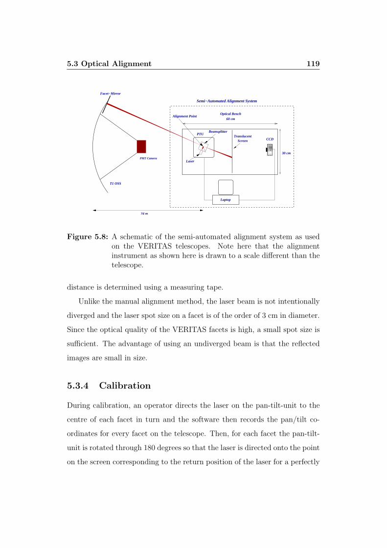
5.3 Optical Alignment 119

TranslucentScreen

Alignment Point

T1 OSS

24 m

Laptop

Laser

Facet−Mirror

PTUBeamsplitter

CCD

PMT Camera

Optical Bench

Semi−Automated Alignment System

60 cm

30 cm

Figure 5.8: A schematic of the semi-automated alignment system as usedon the VERITAS telescopes. Note here that the alignmentinstrument as shown here is drawn to a scale different than thetelescope.

distance is determined using a measuring tape.

Unlike the manual alignment method, the laser beam is not intentionally

diverged and the laser spot size on a facet is of the order of 3 cm in diameter.

Since the optical quality of the VERITAS facets is high, a small spot size is

sufficient. The advantage of using an undiverged beam is that the reflected

images are small in size.

5.3.4 Calibration

During calibration, an operator directs the laser on the pan-tilt-unit to the

centre of each facet in turn and the software then records the pan/tilt co-

ordinates for every facet on the telescope. Then, for each facet the pan-tilt-

unit is rotated through 180 degrees so that the laser is directed onto the point

on the screen corresponding to the return position of the laser for a perfectly

5.3 Optical Alignment 120

Figure 5.9: A picture of semi-automated alignment system system takenfrom above.

aligned mirror. The CCD pixel coordinates of this location are then recorded

by the software, resulting in a process where the precise positioning of the

CCD camera is not important. It also eliminates the complications associated

with distortion produced by the short focal length lens of the CCD. If there

is any movement of any of the system components (pan-tilt-unit, screen,

camera) the calibration must be repeated.

5.3.5 Semi-automated Alignment Procedure

When the system selects a facet for alignment, the pan-tilt-unit points the

laser at the centre of the facet and compares the position of the reflected spot

with the ideal position as determined during the CCD calibration process.

The software then calculates the amount of adjustment required of two of the

5.4 Results 121

three bolts holding that facet to bring the reflected spot to the ideal position.

Instructions are relayed to an assistant located near the facet who must adjust

the bolts manually. Thus the system can be considered a semi-automated

system. Using this semi-automated system an alignment of all 350 facets

can now be completed in ∼ four hours by two people. This is a significant

improvement in terms of manpower and time requirements compared with

the manual method.

5.4 Results

5.4.1 PSF of the VERITAS telescopes

Recently the final telescopes of the VERITAS array were aligned using a

modified version of the original semi-automated alignment system, built at

NUI Galway. After analysis of several CCD images of Polaris, at an elevation

of 31° the FWHM of the PSF of T1 was found to be ∼ 0.08°±5% (Holder

et al., 2006b). Early measurements of the PSFs of T1 of the VERITAS array,

at various elevations, are listed in Table 5.1.

Elevation /° FWHM /°31.0 0.07639.5 0.08051.0 0.09260.5 0.09872.0 0.145

Table 5.1: Results of a recent PSF measurement of T1 of the VERITASarray.

As the VERITAS array has only recently seen first light the task of fully

aligning all the mirror facets of the four telescopes has only recently been

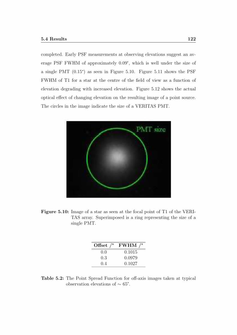
5.4 Results 122

completed. Early PSF measurements at observing elevations suggest an av-

erage PSF FWHM of approximately 0.09°, which is well under the size of

a single PMT (0.15°) as seen in Figure 5.10. Figure 5.11 shows the PSF

FWHM of T1 for a star at the centre of the field of view as a function of

elevation degrading with increased elevation. Figure 5.12 shows the actual

optical effect of changing elevation on the resulting image of a point source.

The circles in the image indicate the size of a VERITAS PMT.

Figure 5.10: Image of a star as seen at the focal point of T1 of the VERI-TAS array. Superimposed is a ring representing the size of asingle PMT.

Offset /° FWHM /°0.0 0.10150.3 0.09790.4 0.1027

Table 5.2: The Point Spread Function for off-axis images taken at typicalobservation elevations of ∼ 65°.

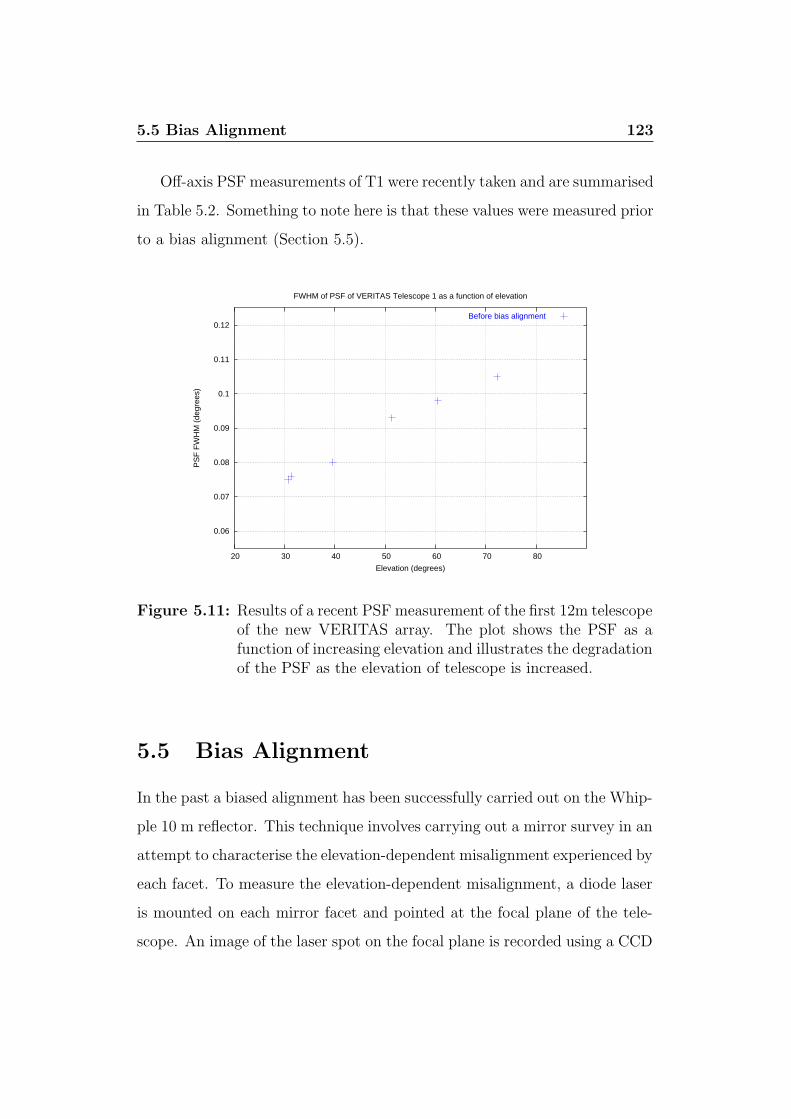
5.5 Bias Alignment 123

Off-axis PSF measurements of T1 were recently taken and are summarised

in Table 5.2. Something to note here is that these values were measured prior

to a bias alignment (Section 5.5).

0.06

0.07

0.08

0.09

0.1

0.11

0.12

20 30 40 50 60 70 80

PS

F F

WH

M (

degr

ees)

Elevation (degrees)

FWHM of PSF of VERITAS Telescope 1 as a function of elevation

Before bias alignment

Figure 5.11: Results of a recent PSF measurement of the first 12m telescopeof the new VERITAS array. The plot shows the PSF as afunction of increasing elevation and illustrates the degradationof the PSF as the elevation of telescope is increased.

5.5 Bias Alignment

In the past a biased alignment has been successfully carried out on the Whip-

ple 10 m reflector. This technique involves carrying out a mirror survey in an

attempt to characterise the elevation-dependent misalignment experienced by

each facet. To measure the elevation-dependent misalignment, a diode laser

is mounted on each mirror facet and pointed at the focal plane of the tele-

scope. An image of the laser spot on the focal plane is recorded using a CCD

5.5 Bias Alignment 124

Figure 5.12: Optical PSF images from T1 of the VERITAS array show-ing the different levels of degradation, as elevation increases,emphasising the importance of the bias alignment procedure.The circle illustrates the 0.15° PMT size.

mounted at the center of the reflector at zero degrees elevation and then at

typical observing elevations (65°). This gives a direct measurement of the

amount each mirror moved during the transition between the home position

(where alignment is carried out) and average observing elevations.

With this information now at hand, modifications can then be made to

the semi-automated alignment system control software that will result in

the alignment system instructing the persons carrying out the alignment to

deliberately misalign the facets while in the home position in such a way that

they self-align as the telescope moves into normal observing positions. This

method is known as “bias alignment” and was successfully carried out on

the Whipple 10 m reflector during the 2001/2002 observing season and was

recently carried out on T1, T2 and T3 of the VERITAS array. Figure 5.13

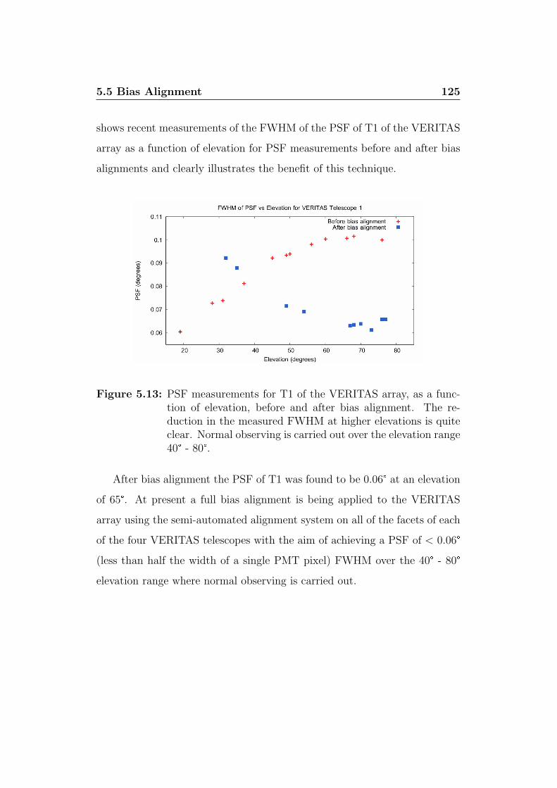
5.5 Bias Alignment 125

shows recent measurements of the FWHM of the PSF of T1 of the VERITAS

array as a function of elevation for PSF measurements before and after bias

alignments and clearly illustrates the benefit of this technique.

Figure 5.13: PSF measurements for T1 of the VERITAS array, as a func-tion of elevation, before and after bias alignment. The re-duction in the measured FWHM at higher elevations is quiteclear. Normal observing is carried out over the elevation range40° - 80°.

After bias alignment the PSF of T1 was found to be 0.06° at an elevation

of 65°. At present a full bias alignment is being applied to the VERITAS

array using the semi-automated alignment system on all of the facets of each

of the four VERITAS telescopes with the aim of achieving a PSF of < 0.06°(less than half the width of a single PMT pixel) FWHM over the 40° - 80°elevation range where normal observing is carried out.

Chapter 6

Iterative Deconvolution of

Whipple Cherenkov Data

6.1 Introduction

Deconvolution is a mathematical technique used in image restoration to re-

verse the effects of convolution on recorded data. The concept of decon-

volution is widely used in the techniques of signal processing and image

processing, particularly in the area of optical astronomy. When an optical

telescope collects an image of a star or galaxy, the light recorded by the in-

strument has been changed by a finite amount, most significantly by slight

imperfections or abberations in the optics of the telescope itself. This is

the process of convolution as mentioned above. For optical instruments the

amount by which the image has been manipulated or convolved, can be cal-

culated by measuring the impulse response, or point spread function (PSF),

of the telescope. The ultimate goal of the deconvolution process is to extract

the original un-degraded image, using knowledge of the PSF and the blurred

image.

6.2 Richardson - Lucy algorithm 127

Since deconvolution is a mathematical operation, many methods have

been developed for use in image restoration projects. However, each method

comes with its own list of advantages and disadvantages. For example,

Fourier-transform methods are successful, but are only so when noise lev-

els in the degraded image are moderate or small (Harris, 1966)(McGlamery,

1966). One of the more popular methods, particularly in optical astron-

omy and medical physics, is known as the Richardson - Lucy algorithm. It

was developed in the early 1970’s independently by Richardson and Lucy

(Richardson, 1972)(Lucy, 1974) and is derived from Bayes’ theorem. Today

it remains a popular method of deconvolution due to its ability to produce

reconstructed images of good quality even in the presence of high noise levels.

This project was the first attempt to apply a deconvolution algorithm of any

kind to imaging atmospheric Cherenkov images in attempt to enhance the

γ-ray signal in Cherenkov data.

6.2 Richardson - Lucy algorithm

The Richardson - Lucy method of deconvolution is an iterative method of

restoring degraded images. The Richardson - Lucy method of deconvolu-

tion has been popular in optical astronomy for many years, and has been

the favored method of image restoration for early degraded Hubble Space

Telescope images (Ricort et al., 1993). The method was developed from

Bayes’ theorem and as such considers images, PSFs, and degraded images,

as probability-frequency functions, and then applies Bayes’ theorem. Because

it relates conditional probabilities, the algorithm takes into account statis-

tical fluctuations in the signal and therefore has the ability to reconstruct

noisy images. Considering this, the Richardson - Lucy algorithm was chosen

6.2 Richardson - Lucy algorithm 128

as the preferred method to apply to Cherenkov images as these images can

contain Poisson fluctuations in the Cherenkov signal, night-sky background

fluctuations and electronic noise fluctuations. Since a major goal of γ-ray

astronomy is the attainment of as high a signal to noise ratio as possible,

this project was deemed worthy in its attempt to improve the signal to noise

ratio of the Whipple telescope. Bayes’ Theorem is a mathematical theorem

based on the definition of conditional probabilities. Conditional probability

is defined as:

P (B|A) =P (A ∩B)

P (A), (6.1)

where P (B|A) is the probability of observing the event B given the fact that

A has occurred, P (A ∩ B) is the probability that both A and B occur, and

P (A) is the probability of B in the first place. Rearranging 6.1 we get:

P (A ∩B) = P (B|A)P (A) = P (A|B)P (B); (6.2)

Rearranging again gives us the formal definition of Bayes’ theorem:

P (B|A) =P (A|B)P (B)

P (A)(6.3)

For our purposes we can assume that a blurred image H can be described by

H=W ∗S, where S is the PSF of the instrument, W is the original image and

∗ signifies the mathematical procedure of convolution. Our task here is to

extract the original image W using what we know of the blurred image and

the PSF. Here we use Bayes’ theorem to express the conditional probability

of an event at Wi given an event at Hk,

P (Wi|Hk) =P (Hk|Wi)P (Wi)∑

j

P (Hk|Wj)P (Wj); (6.4)

6.2 Richardson - Lucy algorithm 129

i = 1, I, j = 1, J, k = 1, K,

The subscripts used here indicate the location of, and value in, the associated

array, for example, Wi refers to the W array value at the ith location in the

array. Hk is an arbitrary cell of H.

By taking all the Hk and their dependence on Wi in accordance with S,

and since P (Wi|Hk) = P (Wi ∩Hk)/P (Hk) (from Equation 6.1), then

P (Wi) =∑

k

P (Wi ∩Hk) =∑

k

P (Wi|Hk)P (Hk) (6.5)

By substituting Equation 6.4 in Equation 6.5 gives

P (Wi) =∑

k

P (Hk|Wi)P (Wi)P (Hk)∑j

P (Hk|Wj)P (Wj)(6.6)

Note that in the right side of this equation, P(Wi), is the desired solution.

Since we don’t know this when starting the deconvolution process, a com-

mon practice (McGlamery & Gray, 1963) is to use an estimate of the P(Wi)

function to obtain, from Equation 6.4, an approximation of P (Wi|Hk). Thus

Equation 6.6 becomes

Pr+1(Wi) = Pr(Wi)∑

k

P (Hk|Wi)P (Hk)∑j

P (Hk|Wj)Pr(Wj)(6.7)

r = 0, 1, 2, . . ..

Equation 6.7 can now be reworked into a more usable form by taking the em-

pirical probability of Wi, i.e. P (Wi) = Wi/W , P (Hk) = Hk/H = Hk/W , and

as the restoration process is conservative, W=H. In addition, P (Hk|Wi) =

6.2 Richardson - Lucy algorithm 130

P (Si,k) = Si,k/S. For a single dimension, Equation 6.7 now becomes

Wi,r+1 = Wi,r

∑

k

Si,kHk∑j

Sj,kWj,r

(6.8)

At this point equation 6.8 can be used to explain the restorative process.

The denominator here is Hk for the current estimate of W. If the Hk estimate

is too big then Hk/Hkestimate < 1. Therefore all of Wi will be adjusted by

this amount as well as being scaled by S.

Equation 6.8 can now be expanded into a two dimensional form, and due

to the finite size of the arrays can be written as:

Wi,j,r+1 = Wi,j,r

e∑m=i

f∑n=j

Hm,nSm−i+1,n−j+1

b∑p=a

d∑q=c

Wq,p,rSm−p+1,n−q+1

, 1 (6.9)

This results in a two dimensional deconvolution iterative process that can

then be applied to Whipple Cherenkov data. This equation was developed

as a algorithmic function/subroutine and written in the C programming lan-

guage. The subroutine was then integrated into the standard analysis soft-

ware prior to the application of the picture and boundary thresholds and

1wherea = (1,m−K + 1)max; b = (m, I)min;

c = (1,n− L + 1)max; d = (n, J)min;

e = i + K− 1; f = j + L− 1;

i = 1, I; j = 1, J r = 0, 1, 2, . . ..

K,L are dimensions of Sk,l and I,J are dimensions of Wi,j

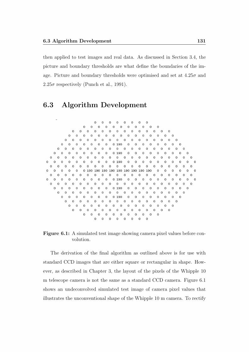
6.3 Algorithm Development 131

then applied to test images and real data. As discussed in Section 3.4, the

picture and boundary thresholds are what define the boundaries of the im-

age. Picture and boundary thresholds were optimised and set at 4.25σ and

2.25σ respectively (Punch et al., 1991).

6.3 Algorithm Development

Figure 6.1: A simulated test image showing camera pixel values before con-volution.

The derivation of the final algorithm as outlined above is for use with

standard CCD images that are either square or rectangular in shape. How-

ever, as described in Chapter 3, the layout of the pixels of the Whipple 10

m telescope camera is not the same as a standard CCD camera. Figure 6.1

shows an undeconvolved simulated test image of camera pixel values that

illustrates the unconventional shape of the Whipple 10 m camera. To rectify

6.3 Algorithm Development 132

the non-rectangular shape of the camera, raw data were mapped into a rect-

angular grid shape and the edges of the hexagonal PMT camera were padded

out with zeros. This padded camera can be seen in Figure 6.2. To test the al-

Figure 6.2: The mapped camera pixels padded with zero pixels

gorithm, a series of simulated images were created and then convolved with

a Gaussian PSF based on the average measured full width half maximum

(FWHM) of the telescope PSF, which was found to be 0.125° (Figure 6.3).

The PSF here is not symmetrical in order for it to be compatible with the

Figure 6.3: PSF used to test deconvolution algorithm. FWHM is 0.125°.Note here that the PSF has been shifted in the same manner asthe camera pixels in Figure 6.2 to ensure correct convolution.

6.3 Algorithm Development 133

shape and pixel layout of the 10 m camera. The convolved image is shown

in Figure 6.4. The effects of convolution can clearly be seen here. Looking

at the blurred or convolved image we can see that the most affected pixels

are those closest to the main non-distorted image pixels. The total amount

of light in the camera remains constant but has been spread out to an extent

as determined by the PSF. The basic shape of the cross of numbers can still

be recognised but it is now much wider. The light in the image has been

spread out, and the role of the Richardson - Lucy algorithm is now to undo

this spreading of light in the image.

Figure 6.4: Camera pixel values after convolution

6.3 Algorithm Development 134

6.3.1 Testing the algorithm

After applying the Richardson - Lucy algorithm to the simulated image and

iterating 20 times, the resulting image is shown in Figure 6.5. The recon-

structed image is clearly much closer to the original image with a small

difference in the worst affected pixel compared to the original values. Any

further iterations of the algorithm on the image did not improve upon the

image as shown.

Figure 6.5: Camera pixel values after deconvolution - 20 iterations

At this point, as can be seen from the images the algorithm was success-

fully deconvolving distinctive patterns on the camera. However, these initial

images did not have any noise added and in reality Cherenkov images are far

from noiseless. To match noise levels in real Cherenkov images, a Gaussian

distribution of random numbers with a standard deviation of 2 was generated

to simulate noise. This noise was added to the convolved images, see Figure

6.3 Algorithm Development 135

6.6 (top), and the deconvolution algorithm was again applied to the simu-

lated data. Figure 6.6 (bottom) shows the effect of applying 20 iterations to

the noisy image.

Looking at the deconvolved noisy image a hot spot of high pixel values,

both positive and negative, has appeared in the top right quadrant of the

camera. Several other large pixel values have also appeared in random regions

of the camera. It was found that this effect was caused by very small negative

values, due to noise fluctuations, that were appearing in the denominator in

Equation 6.9 resulting in large negative values. These random fluctuations

would change from iteration to iteration and appear in random regions of

the camera. For example the large pixel values seen in Figure 6.6 (bottom

image) did not appear in the subsequent iterated image, however a different

hot spot had appeared in a separate part of the camera. To remedy this, just

before the point of applying the algorithm, any negative pixel values were

removed from the image, i.e. they were zeroed out of the image as can be

seen in Figure: 6.7 (top image).

The effect of removing these negative values can be seen in Figure 6.7

(bottom image). Here the random large pixel values are no longer appearing

in the deconvolved images, and the algorithm is performing satisfactorily as

it did before the addition of the random noise.

Further tests show that the algorithm can successfully restore convolved

simulated images close to their original un-degraded form even in the presence

of non-negative random noise. However this condition is only true provided

the blurring component or PSF used to blur the images is known accurately.

For these tests the FWHM value used was 0.125°.

6.3 Algorithm Development 136

Figure 6.6: Camera with noise added before (top) and after (bottom) de-convolution

6.3 Algorithm Development 137

Figure 6.7: Camera with image and noise (no negative values) before (top)and after (bottom) deconvolution

6.4 Observations and Analysis 138

6.4 Observations and Analysis

To test the deconvolution process on real Cherenkov data, a group of 10

ON/OFF Crab nebula pairs were chosen from the 2003/2004 observing sea-

son. These data files are listed in Table 6.1. The selection was chosen as a

PSF measurement had been taken close to the time the data were collected.

The measured FWHM of the PSF varied between 0.12° and 0.14° depending

on the corresponding telescope elevation of between 60° and 80°.

Date ON run id no. OFF run id no.031022 25505 25506031023 25526 25527031120 25738 25739031120 25740 25741031121 25759 25760031121 25761 25762031121 25763 25764031122 25781 25782031122 25783 25784031124 25828 25829

Table 6.1: Selected data file identification numbers of the Crab pairs usedto test deconvolution algorithm

For comparison purposes the data were analysed using the standard Su-

percuts analysis software. The deconvolution algorithm was then incorpo-

rated into the analysis software at the stage before the application of picture

and boundary thresholds as mentioned earlier. Prior to the deconvolution

of the images, the normal analysis procedures were carried out on the data

(including software padding) up to the point of zeroing any negative pixels.

Negative pixels were zeroed in order to avoid errors arising from a small

negative denominator in Equation 6.9. Once all negative pixels have been

6.4 Observations and Analysis 139

eliminated from the image, the deconvolution algorithm was applied to each

image and iterated a number of times. It was found the images converged

after about 14 iterations (i.e. the maximum number of iterations applied to

the images after which the algorithm had no further effect on the image).

The initial impact of the algorithm was the extended length of time the

deconvolution analysis procedure took. This could be as long as 50 to 60

minutes (on a 2 GHz Pentium machine) per ON/OFF run as compared with

the 1 to 2 minutes per ON/OFF run for normal analysis. Once the 14 itera-

tions were completed normal picture and boundary thresholds were applied

to the resulting image, i.e. non-image pixels were zeroed. From this point on

the data were analysed as normal, and the standard Supercuts (Punch et al.,

1991) method of selecting γ-rays were applied.

Not-deconvolved Deconvolved

12.36 σ 9.88 σ

Table 6.2: Standard analysis results from the selected Crab data set usingstandard Supercuts on non-deconvolved data and deconvolveddata. The FWHM of the PSF used to deconvolve was 0.13°

The initial results from this analysis using the standard Supercuts values

showed a reduction in the significance as compared to standard analysis pro-

cedures. Table 6.2 shows the significance found using the standard Super-

cuts and picture and boundary threshold values of 4.25 and 2.25 on non-

deconvolved and deconvolved data. It was expected that a reoptimisation of

the cut values would be required to gain the most out of the image restoration

process. However, upon examination of the camera events before and after

deconvolution, it became apparent that deconvolving the images produces

6.4 Observations and Analysis 140

small islands of signal that were passing the standard picture and boundary

thresholds, see Figure 6.8

6.4.1 Picture and Boundary thresholds

By studying and comparing deconvolved and non-deconvolved images it is

clear that the deconvolution algorithm has by its nature increased the amount

of light in the central region of the image. In other words it has sharpened

the image by gathering part of the image that was previously excluded from

further analysis, by the picture and boundary thresholds, and is now includ-

ing it. The result of this effect is to increase the value of the size parameter of

the image significantly. A further effect of the deconvolution was to increase

the signal, in the same manner, in singular or small groupings or islands of

pixels in the camera (Figure 6.8).

When the signal in these island pixels is sufficient to pass the picture and

boundary thresholds, they are included as image pixels and as such they cause

a candidate γ-ray to be rejected later in the analysis when the parameter

cuts are applied. There is the possibility that the island signals may be an

indication of local muonic components and could provide a means to improve

hadronic/γ discrimination. The presence of the island signals prompted a

full re-optimisation of the picture and boundary threshold levels along with

a re-optimisation of the parameter cuts using the test data mentioned above.

Due to the length of time it takes to deconvolve one data run, it was deemed

impractical to perform a standard picture and boundary optimisation. The

standard method requires that for each picture and boundary value the events

are parameterised once. For this work each picture and boundary value

parameterised dataset would require deconvolving.

This involved modifying the standard analysis code to save the decon-

6.4 Observations and Analysis 141

Figure 6.8: Candidate γ-ray images before (top) & after deconvolution(bottom)

6.4 Observations and Analysis 142

volved Cherenkov images for subsequent input to the optimisation stage.

Then a full range of picture and boundary values was applied to the de-

convolved data and a parameterised data file for each picture and boundary

value then returned. Cut values were then optimised on each of these pa-

rameterised data files.

6.4.2 Cut Optimisation

The standard method of cut optimisation involves varying a single cut value

over a suitable range while all other cuts are held at a predetermined set of

values. Normally the variation in significance, as the upper and lower bounds

of each parameter cut are changed, is plotted. The plots are then used to find

the optimum cut values, i.e. those values for which the statistical significance

of the excess is highest. To test cut values obtained from an optimisation,

the process is repeated on an independent set of data.

In this experiment a different approach to cut optimisation was carried

out. The method involved optimising values for the cuts on length, width,

alpha, length/size and on max 1 and max 2. The cuts were optimised by

producing a five dimensional (one dimension per parameter) distribution of

all the events to be optimised for the ON and OFF data i.e. all events in the

ON and OFF data were binned in five dimensional parameter spaces. The

bin sizes were 0.01° for length and width, 1 ° for alpha, 0.00001° for length/size

and 10 for max 1 and 2. Each distribution was then integrated along each

axis creating a distribution that had a value for the number of events that

passed each particular bin. The significance could then be determined for

each bin using the ON and OFF distributions using the Li & Ma (1983)

method.

The bin containing the peak significance was chosen as the optimised cut

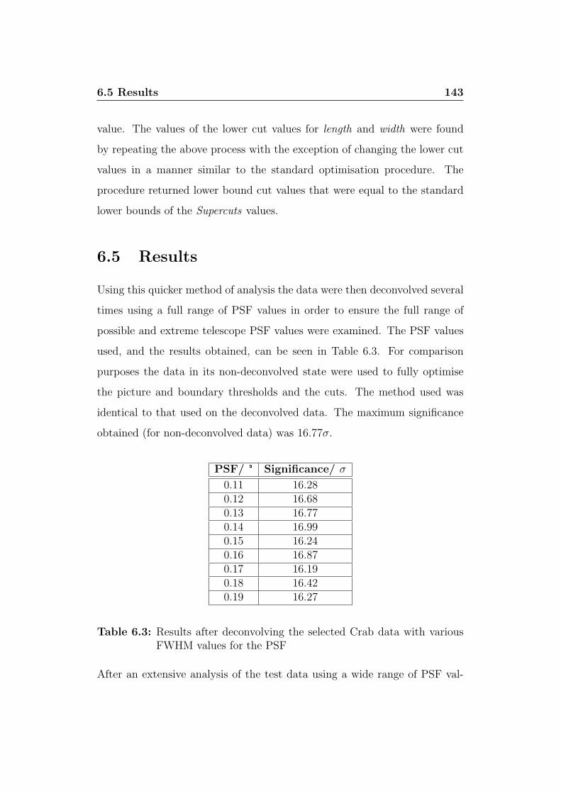
6.5 Results 143

value. The values of the lower cut values for length and width were found

by repeating the above process with the exception of changing the lower cut

values in a manner similar to the standard optimisation procedure. The

procedure returned lower bound cut values that were equal to the standard

lower bounds of the Supercuts values.

6.5 Results

Using this quicker method of analysis the data were then deconvolved several

times using a full range of PSF values in order to ensure the full range of

possible and extreme telescope PSF values were examined. The PSF values

used, and the results obtained, can be seen in Table 6.3. For comparison

purposes the data in its non-deconvolved state were used to fully optimise

the picture and boundary thresholds and the cuts. The method used was

identical to that used on the deconvolved data. The maximum significance

obtained (for non-deconvolved data) was 16.77σ.

PSF/ ° Significance/ σ

0.11 16.280.12 16.680.13 16.770.14 16.990.15 16.240.16 16.870.17 16.190.18 16.420.19 16.27

Table 6.3: Results after deconvolving the selected Crab data with variousFWHM values for the PSF

After an extensive analysis of the test data using a wide range of PSF val-

6.6 Conclusions 144

ues, the deconvolution process proves to be of no benefit with regard to

increasing the significance of the analysis results. For each PSF value, a full

re-optimisation of the picture and boundary levels and parameter cuts was

carried out in order to find the maximum significance. The results of the

optimisation procedures is shown in the form of a contour plot in Figure

6.9. The figure shows contour levels of significance values for various picture

and boundary values for un-deconvolved data (top) and deconvolved data

(bottom). The resulting effect of the deconvolution is to shift the peak in

significance to higher picture and boundary levels. However the peak sig-

nificance of the deconvolved data is not significantly increased compared to

un-deconvolved data. The FWHM value of the PSF used in the plot shown

was 0.14°.Finally, the original cuts and optimised cuts were applied to an inde-

pendent data set for comparison purposes. Using Supercuts a maximum

significance of 10.23σ was found. After applying the optimised cuts to the

un-deconvolved independent data set the significance dropped to 8.71σ, a

reduction of 15% from the Supercuts value. The independent data set was

then deconvolved using the same procedures outlined above. Subsequent to

deconvolution of the independent data set, a significance was 9.41σ returned,

a reduction of 8%.

6.6 Conclusions

The peak signal seen from the independent data set before deconvolution was

10.23σ with picture and boundary thresholds set at 5.00 and 3.00 respectively.

After deconvolution a peak signal of 9.41σ (an 8% decrease) with picture and

boundary thresholds set at 7.00 and 3.50 was found. As mentioned previously

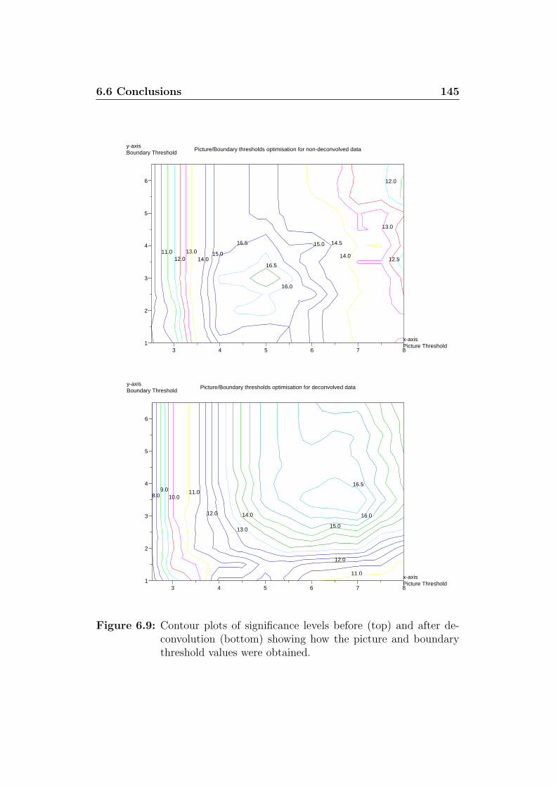
6.6 Conclusions 145

3 4 5 6 7 81

2

3

4

5

6

Picture/Boundary thresholds optimisation for non-deconvolved data

x-axisPicture Threshold

y-axisBoundary Threshold

11.0

12.0

12.0 12.5

13.0

13.014.0

14.0

14.515.0

15.0

15.5

16.0

16.5

3 4 5 6 7 81

2

3

4

5

6

Picture/Boundary thresholds optimisation for deconvolved data

x-axisPicture Threshold

y-axisBoundary Threshold

8.09.0

10.0

11.0

11.0

12.0

12.0

13.0

13.5

14.0

15.0

15.0

16.0

16.5

Figure 6.9: Contour plots of significance levels before (top) and after de-convolution (bottom) showing how the picture and boundarythreshold values were obtained.

6.6 Conclusions 146

the deconvolution process is increasing the amount of light in groupings of

pixels resulting in the necessary re-optimisation of the picture and boundary

thresholds. The effect of this can be seen in the contour plots. In effect

the size of each Cherenkov image has been increased by an amount so as to

require raising the picture and boundary threshold levels by 65% and 55%

respectively. The cut values used to achieve the obtained significance values

are shown in Tables 6.4 and 6.5. Using the optimum cut values found from

optimising the non-deconvolved data with the standard analysis software

gave a significance of 8.71σ.

Cut Value

Length < 0.20°Width < 0.08°Alpha < 9°

Length/size < 0.00032°Max 1 & 2 > 100

Picture 7.00Boundary 3.50

Table 6.4: Optimum cut values for deconvolved data.

Cut Value

Length < 0.22°Width < 0.09°Alpha < 11°

Length/size < 0.00031°Max 1 & 2 > 60

Picture 5.00Boundary 3.00

Table 6.5: Optimum cut values for non-deconvolved data.

It must be made clear that this increase in the size of the image is caused

6.6 Conclusions 147

by the sharpening of the image and the extra light required for this increase

was previously being zeroed out as it was spread across several pixels. In

other words, part of the image signal that was perviously omitted as it was

not high enough to pass the picture and boundary thresholds is now being

included to the final stages of the analysis. Further investigation to deter-

mine the significance of the increase in the average value of the size image

parameter, with respect to the energy of the primary particle, has not been

carried out here.

Something of note here is that optimising the picture and boundary levels

with non-deconvolved data resulted in a peak in significance with the picture

and boundary levels at 5.00 and 3.00. This is an increase of 18% and 33% on

the current picture and boundary level settings used in a standard Supercuts

analysis, and could prompt a need to look at new picture and boundary levels

in the analysis of archived data. The original threshold values were derived

in 1991 (Punch et al., 1991) and have been used with the standard analysis

since then.

The work described here has demonstrated that the iterative deconvolu-

tion of the point spread function from Cherenkov images does not enhance the

sensitivity of the atmospheric Cherenkov imaging technique. It was hoped

that by deconvolving the Cherenkov images in the data set, candidate images

would be sharpened up to the degree that true γ-ray events that were being

rejected by Supercuts would, subsequent to deconvolution, pass the selection

criteria. It was also hoped that non-γ-ray event images would also be sharp-

ened thus revealing detail that would allow enhanced discrimination between

γ-ray events, hadronic events and other noise events.

Chapter 7

Reanalysis of archival data of

the unidentified TeV source

TeV J2032+4130

7.1 Introduction

The unidentified TeV source TeV J2032+4130, located in the Cygnus region,

has been confirmed as a source of very high energy γ-rays (Aharonian et al.,

2005a; Lang et al., 2004). Since its serendipitous discovery by the HEGRA

group in 2002 (Aharonian et al., 2002), TeV J2032+4130 has been the subject

of on-going study. Observations of Cygnus X-3 were taken with the Whip-

ple 10 m imaging atmospheric Cherenkov telescope during the 1989/1990

observing season searching for a γ-ray signal from this crowded region of

sky. However, no γ-ray emission of any kind was detected from Cygnus X-3

(O’Flaherty et al., 1992) and the data were consigned to the archives. At

the time of the original analysis, only a point source analysis at the centre of

the field of view was carried out as this was the standard analysis technique

7.2 Observations 149

at that time.

Following the unexpected detection of TeV J2032+4130 by the HEGRA

group, Lang et al. (2004) carried out an analysis of the Cygnus dataset

over the entire field of view of the telescope. This technique, known as a

two-dimensional analysis (Lessard et al., 2001), yielded a 3.3σ excess at the

position of the source detected by HEGRA and was reported by the authors,

thus TeV J2032+4130 was confirmed as a TeV γ-ray emitter. The levels of

interest in this object motivated a further reanalysis of the archival dataset

here with the aim of improving the significance of the detected signal and

refining the estimated flux levels of this TeV source for the epoch 1989/1990.

This chapter details the methods used in this attempt at increasing the signal

to noise ratio, details the determination of the differential and integral flux

values and presents the results obtained.

7.2 Observations

During the 1988-1990 epoch, observations of Cygnus X-3 were carried out in

the ON/OFF mode. However there were slight differences in the length of

the observation runs as well differences in the PMT camera configuration to

that of the camera configuration used for the analysis described in Chapter

5. For observations of this source a right ascension position that is more

distant than normal, is required for a suitable dark region of sky for the OFF

run and thus avoid a bright region of sky. Subsequently, due to the extended

right ascension position, the length of the observations is altered. In this case

the ON/OFF mode tracked the object for 38 minutes (the ON run), then

over the next 2 minutes the telescope was slewed to a position 40 minutes

later in right ascension and this “dark” region of the sky was tracked for 38

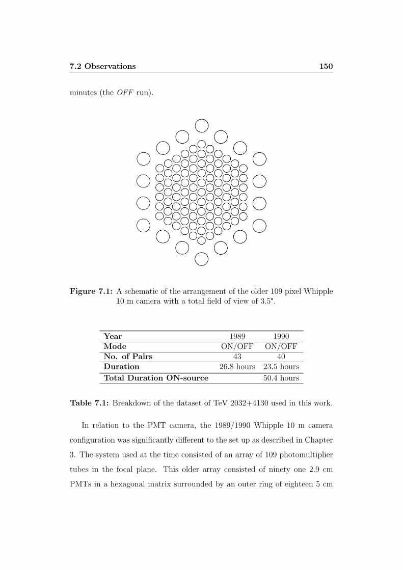
7.2 Observations 150

minutes (the OFF run).

Figure 7.1: A schematic of the arrangement of the older 109 pixel Whipple10 m camera with a total field of view of 3.5°.

Year 1989 1990Mode ON/OFF ON/OFFNo. of Pairs 43 40Duration 26.8 hours 23.5 hours

Total Duration ON-source 50.4 hours

Table 7.1: Breakdown of the dataset of TeV 2032+4130 used in this work.

In relation to the PMT camera, the 1989/1990 Whipple 10 m camera

configuration was significantly different to the set up as described in Chapter

3. The system used at the time consisted of an array of 109 photomultiplier

tubes in the focal plane. This older array consisted of ninety one 2.9 cm

PMTs in a hexagonal matrix surrounded by an outer ring of eighteen 5 cm

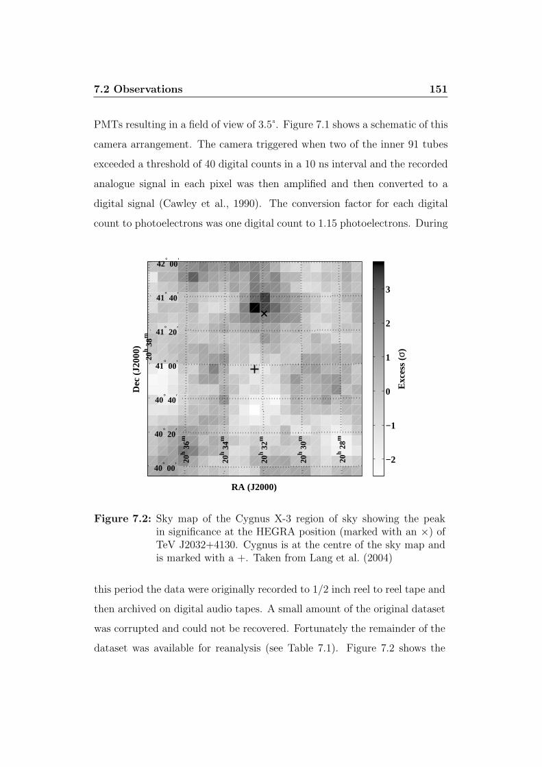
7.2 Observations 151

PMTs resulting in a field of view of 3.5°. Figure 7.1 shows a schematic of this

camera arrangement. The camera triggered when two of the inner 91 tubes

exceeded a threshold of 40 digital counts in a 10 ns interval and the recorded

analogue signal in each pixel was then amplified and then converted to a

digital signal (Cawley et al., 1990). The conversion factor for each digital

count to photoelectrons was one digital count to 1.15 photoelectrons. During

RA (J2000)

Dec

(J2

000)

20h 2

8m

20h 3

0m

20h 3

2m

20h 3

4m

20h 3

6m

20h 3

8m

40° 00′

40° 20′

40° 40′

41° 00′

41° 20′

41° 40′

42° 00′

Exc

ess

(σ)

−2

−1

0

1

2

3

Figure 7.2: Sky map of the Cygnus X-3 region of sky showing the peakin significance at the HEGRA position (marked with an ×) ofTeV J2032+4130. Cygnus is at the centre of the sky map andis marked with a +. Taken from Lang et al. (2004)

this period the data were originally recorded to 1/2 inch reel to reel tape and

then archived on digital audio tapes. A small amount of the original dataset

was corrupted and could not be recovered. Fortunately the remainder of the

dataset was available for reanalysis (see Table 7.1). Figure 7.2 shows the

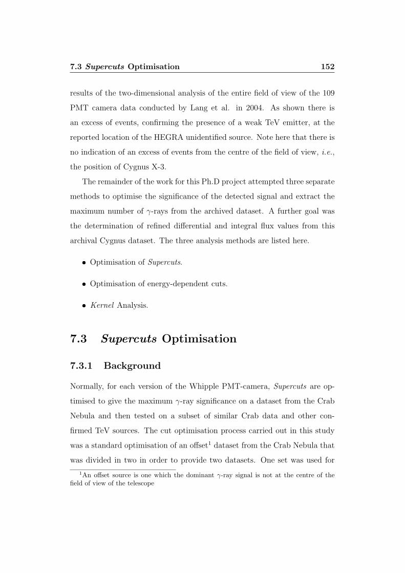
7.3 Supercuts Optimisation 152

results of the two-dimensional analysis of the entire field of view of the 109

PMT camera data conducted by Lang et al. in 2004. As shown there is

an excess of events, confirming the presence of a weak TeV emitter, at the

reported location of the HEGRA unidentified source. Note here that there is

no indication of an excess of events from the centre of the field of view, i.e.,

the position of Cygnus X-3.

The remainder of the work for this Ph.D project attempted three separate

methods to optimise the significance of the detected signal and extract the

maximum number of γ-rays from the archived dataset. A further goal was

the determination of refined differential and integral flux values from this

archival Cygnus dataset. The three analysis methods are listed here.

Optimisation of Supercuts.

Optimisation of energy-dependent cuts.

Kernel Analysis.

7.3 Supercuts Optimisation

7.3.1 Background

Normally, for each version of the Whipple PMT-camera, Supercuts are op-

timised to give the maximum γ-ray significance on a dataset from the Crab

Nebula and then tested on a subset of similar Crab data and other con-

firmed TeV sources. The cut optimisation process carried out in this study

was a standard optimisation of an offset1 dataset from the Crab Nebula that

was divided in two in order to provide two datasets. One set was used for

1An offset source is one which the dominant γ-ray signal is not at the centre of thefield of view of the telescope

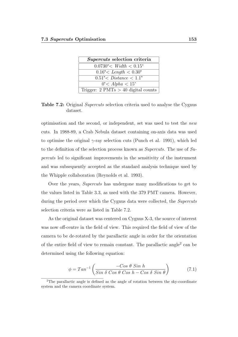
7.3 Supercuts Optimisation 153

Supercuts selection criteria

0.0730°< Width < 0.15°0.16°< Length < 0.30°0.51°< Distance < 1.1°

0°< Alpha < 15°Trigger: 2 PMTs > 40 digital counts

Table 7.2: Original Supercuts selection criteria used to analyse the Cygnusdataset.

optimisation and the second, or independent, set was used to test the new

cuts. In 1988-89, a Crab Nebula dataset containing on-axis data was used

to optimise the original γ-ray selection cuts (Punch et al. 1991), which led

to the definition of the selection process known as Supercuts. The use of Su-

percuts led to significant improvements in the sensitivity of the instrument

and was subsequently accepted as the standard analysis technique used by

the Whipple collaboration (Reynolds et al. 1993).

Over the years, Supercuts has undergone many modifications to get to

the values listed in Table 3.3, as used with the 379 PMT camera. However,

during the period over which the Cygnus data were collected, the Supercuts

selection criteria were as listed in Table 7.2.

As the original dataset was centered on Cygnus X-3, the source of interest

was now off-centre in the field of view. This required the field of view of the

camera to be de-rotated by the parallactic angle in order for the orientation

of the entire field of view to remain constant. The parallactic angle2 can be

determined using the following equation:

φ = Tan−1

( −Cos θ Sin h

Sin δ Cos θ Cos h− Cos δ Sin θ

)(7.1)

2The parallactic angle is defined as the angle of rotation between the sky-coordinatesystem and the camera coordinate system.

7.3 Supercuts Optimisation 154

where φ is the parallactic angle, θ is the latitude of the Whipple 10 m tele-

scope, δ is the declination coordinates of the source being observed and h is

the hour angle of the source. After a two-dimensional analysis of the Cygnus

dataset, Lang et al. (2004) reported an excess with a significance of 3.3σ

at the reported HEGRA position. At that time no attempt was made to

optimise the selection criteria. Fortunately, during the same epoch, a series

of off-axis observations were made on the Crab Nebula. During these ob-

Figure 7.3: Length distribution of 1 TeV simulated γ-rays from a centeredsource and from a source with a 1° offset position in the fieldof view.

servations the position of the Crab Nebula was deliberately offset from the

centre of the field of view by 1° in order to determine the off-axis efficiency

of the telescope. This Crab dataset, like the Cygnus dataset, was archived

7.3 Supercuts Optimisation 155

as binary files on magnetic tapes. The entire 109-pixel camera database was

transferred to digital audio tape during the 1990’s. It was from these tapes

that the archived data were retrieved in 2004. Unfortunately there was only

0 0.2 0.4 0.6 0.8 1 1.2 1.4 1.60

50

100

150

200

250

Distance (deg)

Num

ber

of e

vent

s

Figure 7.4: Distance distributions for a database of 1 TeV simulated γ-rayswith a 1° offset position in the field of view.

a limited amount of Crab offset data retrievable from the digital audio tapes.

In total, 13 pairs ( ∼ 5 hrs) of 1° offset data were obtained from the archives.

Although not an ideal amount of data to attempt a cut optimisation, it

was deemed to be a worth-while task as, if successful, it would result in an

improvement of the significance of the detection.

A further motivation for re-optimisation of Supercuts for an offset source

was the effect the actual distance of the source, from the centre of the field of

7.3 Supercuts Optimisation 156

view, had on some of the image parameters. In particular length values can

be ∼ 25% longer for offset sources. Figure 7.3 shows the length distributions

of simulated 1 TeV showers for an on-axis source and a source offset by 1°from the centre of the field of view. The difference in the length distribution

for on-axis and offset source can be clearly seen. A similar effect is seen when

the width parameter distributions are examined. However the effect is not

as pronounced as for length. The distance parameter is also altered with an

off-axis source but will be discussed at a later stage.

7.3.2 Optimisation Method and Results

The optimisation method used in this piece of work was the single parameter

variation method, where a particular parameter is set to an initial starting

value and then adjusted over a reasonable range in order to search for the

optimum value for that parameter. This initial optimum value is the first best

estimate value and then replaces the initial starting value. The procedure is

then repeated for each individual parameter. The whole procedure is then

repeated to find the next best estimate, which then replaces the previous

best estimate. This operation is then continued until each new best estimate

value converges on its optimised values.

Upon concluding the optimisation procedure, it was found that the op-

timum values converged to values close to the original Supercuts. However,

when these new optimised cuts were applied to the independent dataset a

reduction in significance was observed. This suggests that the original cuts

were correctly optimised to begin with. The optimisation procedure was car-

ried out initially on data with the signal from the Crab Nebula centred in

the field of view. It was then applied to Crab data offset by 1° in the field

of view and a final attempt was also made to optimise the cuts using the

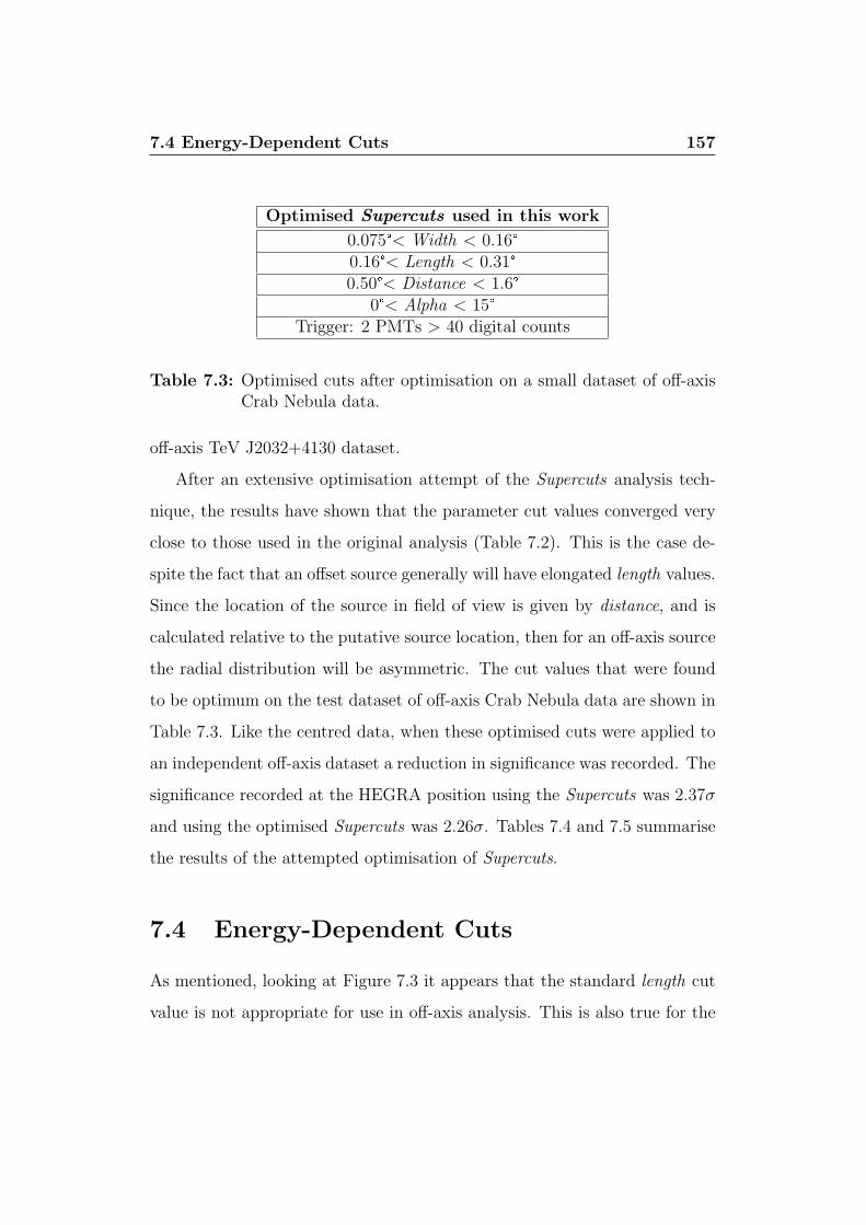
7.4 Energy-Dependent Cuts 157

Optimised Supercuts used in this work

0.075°< Width < 0.16°0.16°< Length < 0.31°0.50°< Distance < 1.6°

0°< Alpha < 15°Trigger: 2 PMTs > 40 digital counts

Table 7.3: Optimised cuts after optimisation on a small dataset of off-axisCrab Nebula data.

off-axis TeV J2032+4130 dataset.

After an extensive optimisation attempt of the Supercuts analysis tech-

nique, the results have shown that the parameter cut values converged very

close to those used in the original analysis (Table 7.2). This is the case de-

spite the fact that an offset source generally will have elongated length values.

Since the location of the source in field of view is given by distance, and is

calculated relative to the putative source location, then for an off-axis source

the radial distribution will be asymmetric. The cut values that were found

to be optimum on the test dataset of off-axis Crab Nebula data are shown in

Table 7.3. Like the centred data, when these optimised cuts were applied to

an independent off-axis dataset a reduction in significance was recorded. The

significance recorded at the HEGRA position using the Supercuts was 2.37σ

and using the optimised Supercuts was 2.26σ. Tables 7.4 and 7.5 summarise

the results of the attempted optimisation of Supercuts.

7.4 Energy-Dependent Cuts

As mentioned, looking at Figure 7.3 it appears that the standard length cut

value is not appropriate for use in off-axis analysis. This is also true for the

7.4 Energy-Dependent Cuts 158

Standard Supercuts Significance ResultsSource Crab On-axis Crab Off-axis TeV J2032

Test data 11.84σ 4.19σ —–Independent data 10.79σ 3.08σ —–

All data —– —– 3.98σ

Optimised Supercuts Significance ResultsSource Crab On-axis Crab Off-axis TeV J2032

Test data 12.74σ 4.38σ —–Independent data 8.37σ 3.07σ —–

All data —– —– 3.89σ

Table 7.4: Summary of significance results obtained using Supercuts andthe optimisation of Supercuts as described in the text.

Standard Supercuts Rate ResultsSource Crab On-axis Crab Off-axis TeV J2032

Test data 0.85±0.07 0.28±0.06 —–Independent data 0.73±0.07 0.23±0.07 —–

All data —– —– 0.08±0.02

Optimised Supercuts Rate ResultsSource Crab On-axis Crab Off-axis TeV J2032

Test data 0.31±0.07 0.31±0.07 —–Independent data 0.50±0.06 0.22±0.07 —–

All data —– —– 0.04±0.02

Table 7.5: Summary of the rate (γ min−1) values obtained using standardSupercuts and optimised Supercuts.

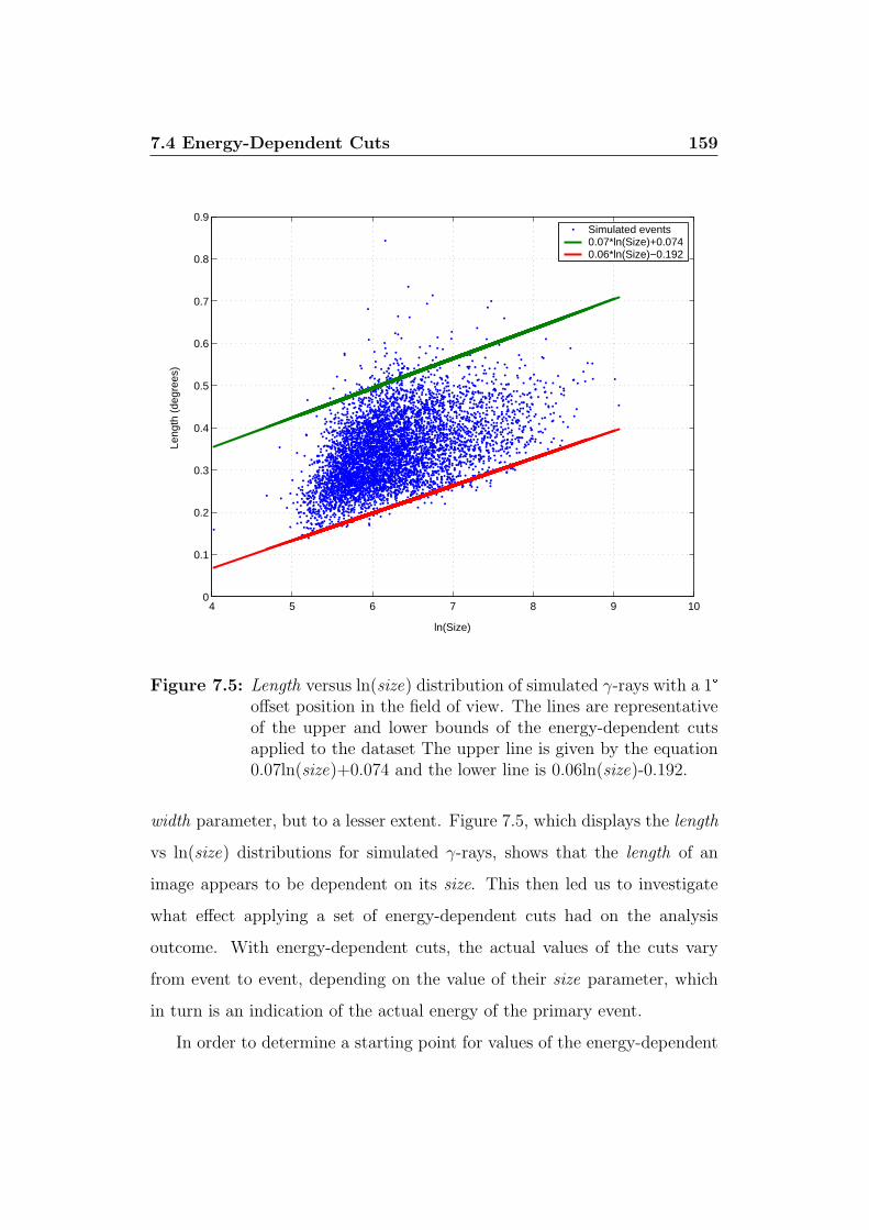
7.4 Energy-Dependent Cuts 159

4 5 6 7 8 9 100

0.1

0.2

0.3

0.4

0.5

0.6

0.7

0.8

0.9

ln(Size)

Leng

th (

degr

ees)

Simulated events0.07*ln(Size)+0.0740.06*ln(Size)−0.192

Figure 7.5: Length versus ln(size) distribution of simulated γ-rays with a 1°offset position in the field of view. The lines are representativeof the upper and lower bounds of the energy-dependent cutsapplied to the dataset The upper line is given by the equation0.07ln(size)+0.074 and the lower line is 0.06ln(size)-0.192.

width parameter, but to a lesser extent. Figure 7.5, which displays the length

vs ln(size) distributions for simulated γ-rays, shows that the length of an

image appears to be dependent on its size. This then led us to investigate

what effect applying a set of energy-dependent cuts had on the analysis

outcome. With energy-dependent cuts, the actual values of the cuts vary

from event to event, depending on the value of their size parameter, which

in turn is an indication of the actual energy of the primary event.

In order to determine a starting point for values of the energy-dependent

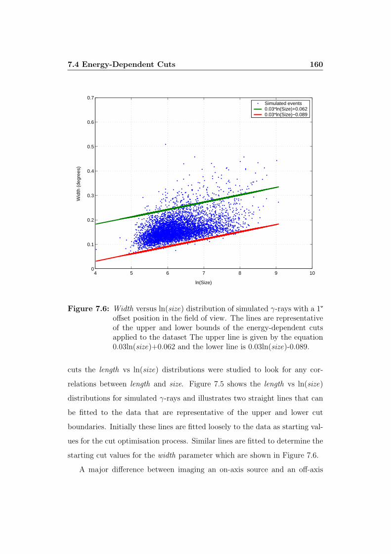
7.4 Energy-Dependent Cuts 160

4 5 6 7 8 9 100

0.1

0.2

0.3

0.4

0.5

0.6

0.7

ln(Size)

Wid

th (

degr

ees)

Simulated events0.03*ln(Size)+0.0620.03*ln(Size)−0.089

Figure 7.6: Width versus ln(size) distribution of simulated γ-rays with a 1°offset position in the field of view. The lines are representativeof the upper and lower bounds of the energy-dependent cutsapplied to the dataset The upper line is given by the equation0.03ln(size)+0.062 and the lower line is 0.03ln(size)-0.089.

cuts the length vs ln(size) distributions were studied to look for any cor-

relations between length and size. Figure 7.5 shows the length vs ln(size)

distributions for simulated γ-rays and illustrates two straight lines that can

be fitted to the data that are representative of the upper and lower cut

boundaries. Initially these lines are fitted loosely to the data as starting val-

ues for the cut optimisation process. Similar lines are fitted to determine the

starting cut values for the width parameter which are shown in Figure 7.6.

A major difference between imaging an on-axis source and an off-axis

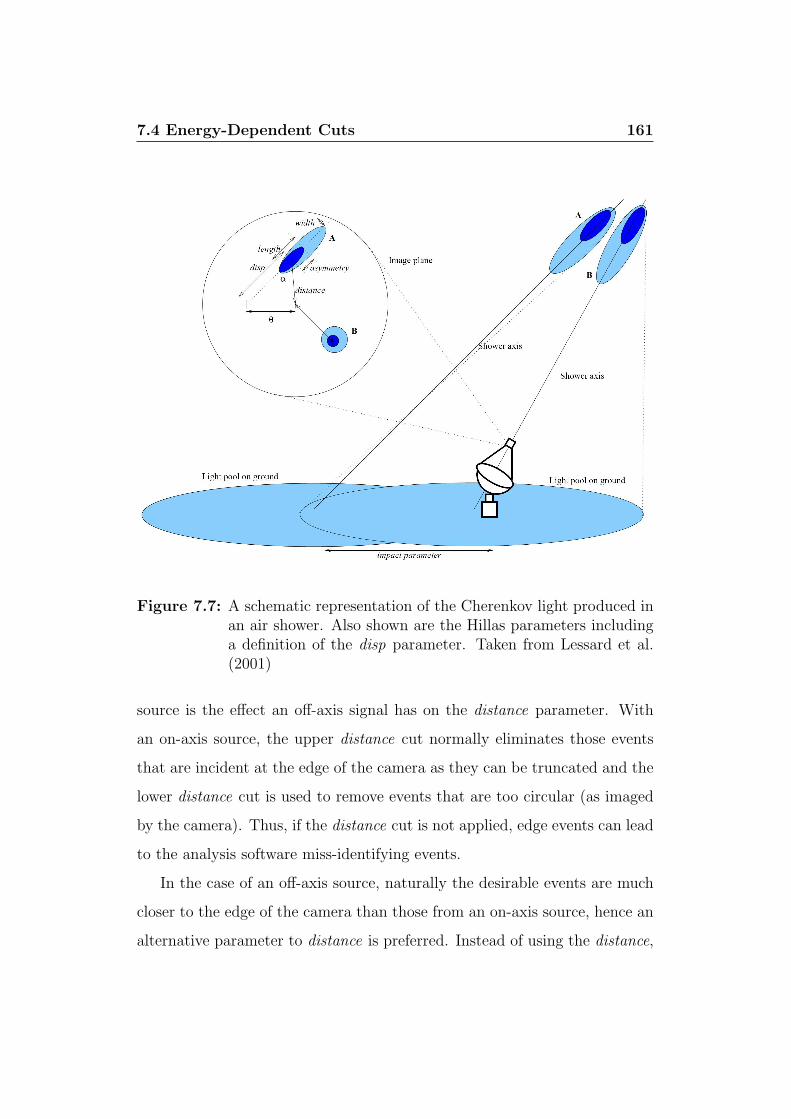
7.4 Energy-Dependent Cuts 161

Figure 7.7: A schematic representation of the Cherenkov light produced inan air shower. Also shown are the Hillas parameters includinga definition of the disp parameter. Taken from Lessard et al.(2001)

source is the effect an off-axis signal has on the distance parameter. With

an on-axis source, the upper distance cut normally eliminates those events

that are incident at the edge of the camera as they can be truncated and the

lower distance cut is used to remove events that are too circular (as imaged

by the camera). Thus, if the distance cut is not applied, edge events can lead

to the analysis software miss-identifying events.

In the case of an off-axis source, naturally the desirable events are much

closer to the edge of the camera than those from an on-axis source, hence an

alternative parameter to distance is preferred. Instead of using the distance,

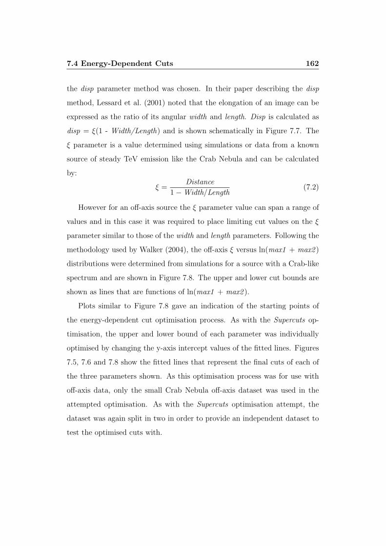
7.4 Energy-Dependent Cuts 162

the disp parameter method was chosen. In their paper describing the disp

method, Lessard et al. (2001) noted that the elongation of an image can be

expressed as the ratio of its angular width and length. Disp is calculated as

disp = ξ(1 - Width/Length) and is shown schematically in Figure 7.7. The

ξ parameter is a value determined using simulations or data from a known

source of steady TeV emission like the Crab Nebula and can be calculated

by:

ξ =Distance

1−Width/Length(7.2)

However for an off-axis source the ξ parameter value can span a range of

values and in this case it was required to place limiting cut values on the ξ

parameter similar to those of the width and length parameters. Following the

methodology used by Walker (2004), the off-axis ξ versus ln(max1 + max2 )

distributions were determined from simulations for a source with a Crab-like

spectrum and are shown in Figure 7.8. The upper and lower cut bounds are

shown as lines that are functions of ln(max1 + max2 ).

Plots similar to Figure 7.8 gave an indication of the starting points of

the energy-dependent cut optimisation process. As with the Supercuts op-

timisation, the upper and lower bound of each parameter was individually

optimised by changing the y-axis intercept values of the fitted lines. Figures

7.5, 7.6 and 7.8 show the fitted lines that represent the final cuts of each of

the three parameters shown. As this optimisation process was for use with

off-axis data, only the small Crab Nebula off-axis dataset was used in the

attempted optimisation. As with the Supercuts optimisation attempt, the

dataset was again split in two in order to provide an independent dataset to

test the optimised cuts with.

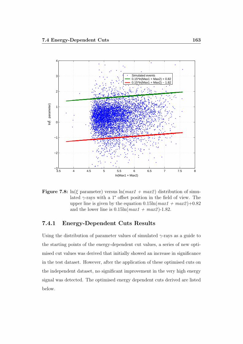
7.4 Energy-Dependent Cuts 163

3.5 4 4.5 5 5.5 6 6.5 7 7.5 8−3

−2

−1

0

1

2

3

4

ln(Max1 + Max2)

ln(

pa

ram

eter

)

Simulated events0.15*ln(Max1 + Max2) + 0.820.15*ln(Max1 + Max2) − 1.82

ξ

Figure 7.8: ln(ξ parameter) versus ln(max1 + max2 ) distribution of simu-lated γ-rays with a 1° offset position in the field of view. Theupper line is given by the equation 0.15ln(max1 + max2 )+0.82and the lower line is 0.15ln(max1 + max2 )-1.82.

7.4.1 Energy-Dependent Cuts Results

Using the distribution of parameter values of simulated γ-rays as a guide to

the starting points of the energy-dependent cut values, a series of new opti-

mised cut values was derived that initially showed an increase in significance

in the test dataset. However, after the application of these optimised cuts on

the independent dataset, no significant improvement in the very high energy

signal was detected. The optimised energy dependent cuts derived are listed

below.

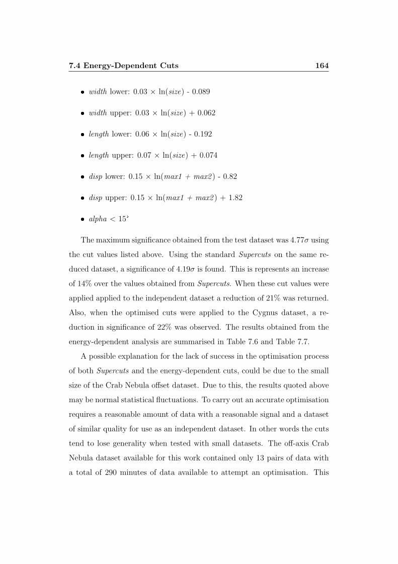
7.4 Energy-Dependent Cuts 164

width lower: 0.03 × ln(size) - 0.089

width upper: 0.03 × ln(size) + 0.062

length lower: 0.06 × ln(size) - 0.192

length upper: 0.07 × ln(size) + 0.074

disp lower: 0.15 × ln(max1 + max2 ) - 0.82

disp upper: 0.15 × ln(max1 + max2 ) + 1.82

alpha < 15°

The maximum significance obtained from the test dataset was 4.77σ using

the cut values listed above. Using the standard Supercuts on the same re-

duced dataset, a significance of 4.19σ is found. This is represents an increase

of 14% over the values obtained from Supercuts. When these cut values were

applied applied to the independent dataset a reduction of 21% was returned.

Also, when the optimised cuts were applied to the Cygnus dataset, a re-

duction in significance of 22% was observed. The results obtained from the

energy-dependent analysis are summarised in Table 7.6 and Table 7.7.

A possible explanation for the lack of success in the optimisation process

of both Supercuts and the energy-dependent cuts, could be due to the small

size of the Crab Nebula offset dataset. Due to this, the results quoted above

may be normal statistical fluctuations. To carry out an accurate optimisation

requires a reasonable amount of data with a reasonable signal and a dataset

of similar quality for use as an independent dataset. In other words the cuts

tend to lose generality when tested with small datasets. The off-axis Crab

Nebula dataset available for this work contained only 13 pairs of data with

a total of 290 minutes of data available to attempt an optimisation. This

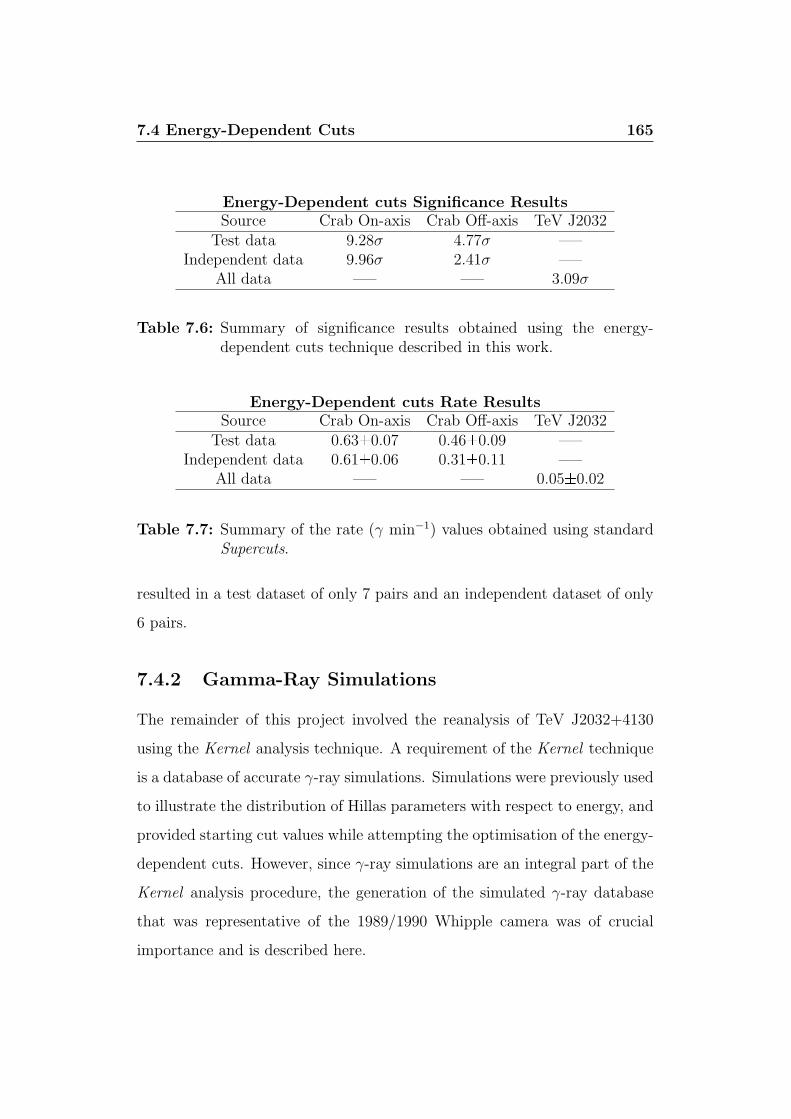
7.4 Energy-Dependent Cuts 165

Energy-Dependent cuts Significance ResultsSource Crab On-axis Crab Off-axis TeV J2032

Test data 9.28σ 4.77σ —–Independent data 9.96σ 2.41σ —–

All data —– —– 3.09σ

Table 7.6: Summary of significance results obtained using the energy-dependent cuts technique described in this work.

Energy-Dependent cuts Rate ResultsSource Crab On-axis Crab Off-axis TeV J2032

Test data 0.63±0.07 0.46±0.09 —–Independent data 0.61±0.06 0.31±0.11 —–

All data —– —– 0.05±0.02

Table 7.7: Summary of the rate (γ min−1) values obtained using standardSupercuts.

resulted in a test dataset of only 7 pairs and an independent dataset of only

6 pairs.

7.4.2 Gamma-Ray Simulations

The remainder of this project involved the reanalysis of TeV J2032+4130

using the Kernel analysis technique. A requirement of the Kernel technique

is a database of accurate γ-ray simulations. Simulations were previously used

to illustrate the distribution of Hillas parameters with respect to energy, and

provided starting cut values while attempting the optimisation of the energy-

dependent cuts. However, since γ-ray simulations are an integral part of the

Kernel analysis procedure, the generation of the simulated γ-ray database

that was representative of the 1989/1990 Whipple camera was of crucial

importance and is described here.

7.4 Energy-Dependent Cuts 166

The Monte Carlo simulations used in this work were generated by the

GrISU (Grinnell - Iowa State University) simulations package (Duke & LeBo-

hec, 2006). The GrISU package was developed to produce simulations for

use with the VERITAS experiment and can be separated into three sections;

extensive air shower simulation, Cherenkov emission simulation and the sim-

ulation of the detector in question. The extensive air shower simulation

generation is carried out by a modified version of the Kascade extensive air

shower simulation software developed by Kertzman & Sembroski (1994).

Kascade uses a model of the atmosphere, follows each particle of the

extensive air shower until it reaches ground level, and builds a three dimen-

sional map of every particle’s trajectory. The next stage of the simulations

process sees the Cherenkf software use the three dimensional map, gener-

ated by Kascade, to simulate Cherenkov emission from each particle as it

passes through the model atmosphere until it interacts, decays, or reaches

ground level. The final part of the simulations package models the detection

of the Cherenkov radiation by the Whipple 10 m telescope (or the VERI-

TAS array depending on the configuration file3 used). The software used

in this instance is the GrISUDet program. At this point each Cherenkov

photon is traced as it is reflected off the mirror facets and on to the PMT

camera. GrISUDet then models the charge pulses produced by the PMTs

and associated electronics. As the package was developed for the VERITAS

experiment, the detector simulation section of the package is geared towards

simulating the response of the VERITAS detectors and the later configura-

tions of the Whipple camera, i.e. the 379 PMT configuration used from 2003

to the present.

Since the TeV J2032+4130 dataset was obtained during 1989-1990, when

3Configuration files contain information relevant to the instrument whose response isbeing simulated e.g. no. of PMTs, PMT gains, PMT locations etc.

7.4 Energy-Dependent Cuts 167

Technical information required to accurately simulate theresponse of the 109 PMT Whipple camera to simulated EAS

PMT threshold in mVPMT current gainMinimum number of channels to trigger the cameraEquivalent system impedanceQuantum efficiency curve (QE as a function of wavelength)Mirror reflectivity curve (Reflectivity as a function of wavelength)X, Y coordinates of each pixel in the focal plane of cameraEach PMT radiusNo. of PMTs surrounding each individual PMT (Nearest neighbours)A list of Each PMTs nearest neighbours ID numberMirror reflectivity degradation factor

Table 7.8: Summary of the technical information required for the modifica-tion of the 379 PMT camera to the 109 PMT camera.

the 109 PMT Whipple camera had very different characteristics, there was

no configuration file available for the 109 PMT camera. Because of this, some

effort was made to modify the configuration file of the 379 PMT camera to

produce a configuration file for the 109 PMT camera by piecing together

specific technical information from various areas.

7.4.3 Simulations for off-axis sensitivity of the 109 PMT

Whipple Camera

The GrISU simulations package has several user-changeable pilot files that

can be used with or without modification if so desired. Each pilot file contains

the input parameters for each different section of the simulation process. For

example, the pilot file for Kascade contains details on how many showers

to create, the energy range to be used, the type of particle, etc. The pilot

7.4 Energy-Dependent Cuts 168

file for GrISUDet tells the software which detector configuration file to use

while simulating the detector response. It also contains information regarding

where the simulated source is in the field of view, the number of pedestal

events to record and the noise characteristics of the field of view. Most of

these variables are quite straight-forward to adjust and generally the detector

configuration file is chosen from a database of files and depends on which

generation of telescope is under study.

109 PMT Configuration File

As this work required the first application of GrISU simulations package rel-

ative to the 109 camera, a suitable PMT configuration file was required in

order to generate an accurate database of simulations for use with the Ker-

nel analysis software. Camera configuration files contain details, amongst an

abundance of other information, regarding PMT thresholds, PMT gain, mir-

ror reflectivities, pixel size, spacing and position. Table 7.8 lists the technical

specifics required to generate a suitable camera configuration file to simulate

the response of the 109 PMT camera. Most of the information regarding

pixel positions, nearest neighbours, quantum efficiency and size, etc., were

obtained from files associated with the older ISU simulations software (Duke,

2005)(Kildea, 2005)(Sembroski, 2005).

Along with these details there were several other important elements to

be gathered. Of crucial importance were details regarding the performance

of the electronics components associated with the 109 PMT camera, i.e. the

PMT triggering thresholds, the system impedance and the PMT current gain.

Of these, the triggering threshold was determined by looking at archived

observer log sheets and old bias curves and was estimated at 83 mV. The

7.4 Energy-Dependent Cuts 169

equivalent system impedance4 was taken to be 152 Ω. This value was taken

from a modified configuration file for the 1995 camera set as supplied by

(Schroedter, 2005) and was based on camera measurements taken in 1994.

Since the queued analogue to digital converters (QADCs) were the same

in the 109 camera, the QADC input impedance and the QADC conversion

factor were taken to be the same as that for the 1995 camera, i.e. 50 Ω and

0.25 respectively. The gain in e− per photoelectron (pe) for the 109 PMT

camera was found to be 0.59 × 106 and was derived from the dc/pe (digital

counts per photoelectron) ratio of 1.15 as reported in Hillas et al. (1998)

using Equation 7.3.

dc/pe =Charge in pC × System Impedance

QADC impedance×QADC conversion factor(7.3)

There were also further modifications to be made to ensure the database of

γ-ray simulations were an accurate representation of real γ-rays . The simu-

lated night sky noise was set so it matched the observed night sky pedestal

variations (Section 3.3.4) as seen in the data. A good match was found with

simulated noise levels set at 380 photoelectrons ns−1m−2str−1 in the simula-

tion pilot files resulting in a matching of the average pedvar values of ∼ 3.14

digital counts.

In addition, the mirror degradation factor was adjusted so it matched the

event size threshold as seen in Figure 7.9. Degradation in mirror reflectivity

can help explain a high energy threshold as well as a decline in statistical

significance (Reynolds et al., 1993). The optimum value for the reflectivity

degradation factor, that gave a good match to the real data with the size

distribution, was 0.54. This low degradation factor can be supported by ob-

4Conversion factor in ohm between amps on the output of the PMT voltages on theanalogue signal processors.

7.4 Energy-Dependent Cuts 170

0

0.05

0.1

0.15

0.2

100 1000

Fra

ctio

n of

eve

nts

Size / degrees

Distribution of Size

ON - OFFSimulations

Figure 7.9: Size distributions of real and simulated events showing thematching peak number of events in the corresponding size binafter the reflectivity degradation factor in the simulations pack-age has been changed to 0.54.

served reflectivity degradation at that epoch. Prior to these observations, the

mirror facets were last re-coated in 1988. Hence, it is reasonable to assume

that, after extended exposure to harsh weather conditions, the mirrors’ abil-

ity to reflect faint flashes of Cherenkov light would be diminished. Further

evidence that supports the reduced reflectivity factor comes in the form of

a drop in the Crab Nebula γ-ray rate over that time period (Lang et al.,

1991). In their work, the authors reported γ-ray rates of 272.9 γ min−1 for

the epoch 1988 to 1989, 227.5 γ min−1 for the epoch 1989 to 1990 and 174.0

γ min−1 for the epoch 1990 to 1991.

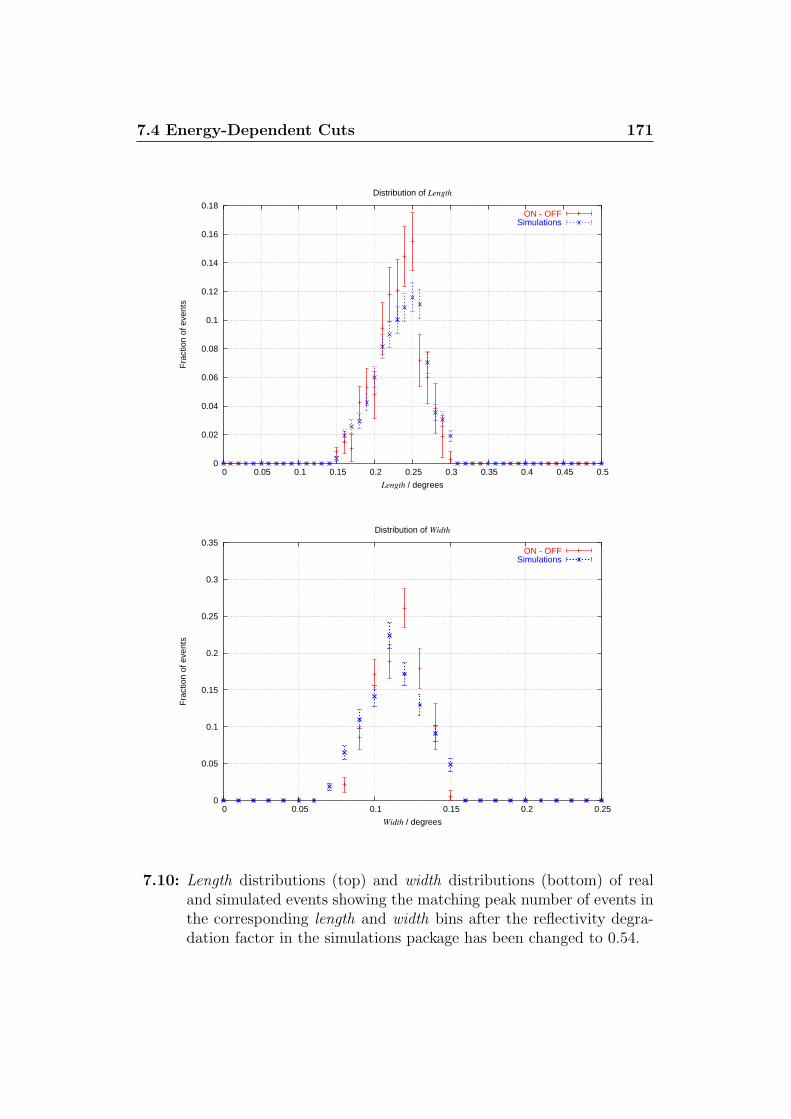
7.4 Energy-Dependent Cuts 171

0

0.02

0.04

0.06

0.08

0.1

0.12

0.14

0.16

0.18

0 0.05 0.1 0.15 0.2 0.25 0.3 0.35 0.4 0.45 0.5

Fra

ctio

n of

eve

nts

Length / degrees

Distribution of Length

ON - OFFSimulations

0

0.05

0.1

0.15

0.2

0.25

0.3

0.35

0 0.05 0.1 0.15 0.2 0.25

Fra

ctio

n of

eve

nts

Width / degrees

Distribution of Width

ON - OFFSimulations

7.10: Length distributions (top) and width distributions (bottom) of realand simulated events showing the matching peak number of events inthe corresponding length and width bins after the reflectivity degra-dation factor in the simulations package has been changed to 0.54.

7.4 Energy-Dependent Cuts 172

0

100

200

300

400

500

600

0 0.2 0.4 0.6 0.8 1 1.2 1.4

Num

ber

of e

vent

s

Distance / degrees

Distribution of Distance

SimulationsReal data

0

0.02

0.04

0.06

0.08

0 10 20 30 40 50

Fra

ctio

n of

eve

nts

Alpha / degrees

Distribution of Alpha

ON - OFFSimulations

7.11: Distance distributions (top) and alpha distributions (bottom) distri-butions of real and simulated events showing a good match betweenreal and simulated events after the reflectivity degradation factor inthe simulations package has been changed to 0.54.

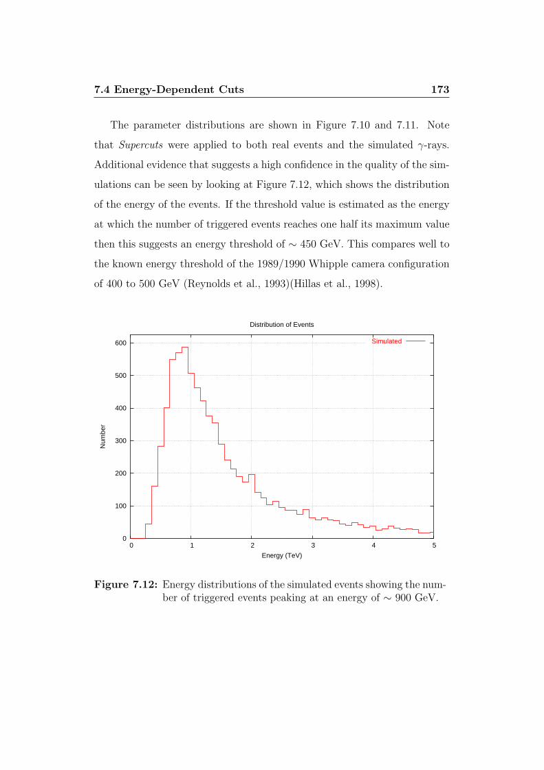
7.4 Energy-Dependent Cuts 173

The parameter distributions are shown in Figure 7.10 and 7.11. Note

that Supercuts were applied to both real events and the simulated γ-rays.

Additional evidence that suggests a high confidence in the quality of the sim-

ulations can be seen by looking at Figure 7.12, which shows the distribution

of the energy of the events. If the threshold value is estimated as the energy

at which the number of triggered events reaches one half its maximum value

then this suggests an energy threshold of ∼ 450 GeV. This compares well to

the known energy threshold of the 1989/1990 Whipple camera configuration

of 400 to 500 GeV (Reynolds et al., 1993)(Hillas et al., 1998).

0

100

200

300

400

500

600

0 1 2 3 4 5

Num

ber

Energy (TeV)

Distribution of Events

Simulated

Figure 7.12: Energy distributions of the simulated events showing the num-ber of triggered events peaking at an energy of ∼ 900 GeV.

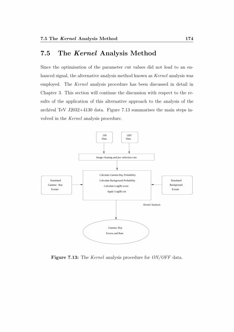
7.5 The Kernel Analysis Method 174

7.5 The Kernel Analysis Method

Since the optimisation of the parameter cut values did not lead to an en-

hanced signal, the alternative analysis method known as Kernel analysis was

employed. The Kernel analysis procedure has been discussed in detail in

Chapter 3. This section will continue the discussion with respect to the re-

sults of the application of this alternative approach to the analysis of the

archival TeV J2032+4130 data. Figure 7.13 summarises the main steps in-

volved in the Kernel analysis procedure.

Simulated

Calculate Gamma Ray Probability

Calculate Background Probability

Calculate Log(R) score

Apply Log(R) cut

Gamma−Ray

Excess and Rate

Kernel Analysis

Gamma− Ray

Events

Simulated

Background

Events

ONData

OFFData

Image cleaning and pre−selection cuts

Figure 7.13: The Kernel analysis procedure for ON/OFF data.

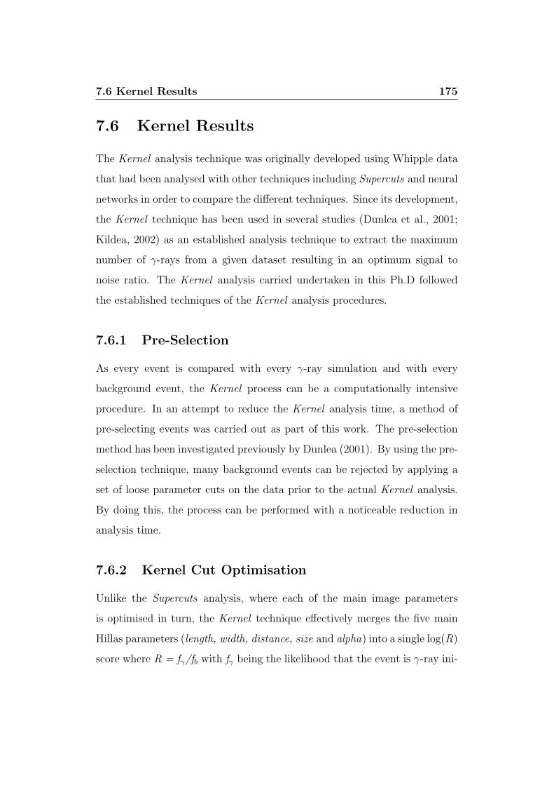
7.6 Kernel Results 175

7.6 Kernel Results

The Kernel analysis technique was originally developed using Whipple data

that had been analysed with other techniques including Supercuts and neural

networks in order to compare the different techniques. Since its development,

the Kernel technique has been used in several studies (Dunlea et al., 2001;

Kildea, 2002) as an established analysis technique to extract the maximum

number of γ-rays from a given dataset resulting in an optimum signal to

noise ratio. The Kernel analysis carried undertaken in this Ph.D followed

the established techniques of the Kernel analysis procedures.

7.6.1 Pre-Selection

As every event is compared with every γ-ray simulation and with every

background event, the Kernel process can be a computationally intensive

procedure. In an attempt to reduce the Kernel analysis time, a method of

pre-selecting events was carried out as part of this work. The pre-selection

method has been investigated previously by Dunlea (2001). By using the pre-

selection technique, many background events can be rejected by applying a

set of loose parameter cuts on the data prior to the actual Kernel analysis.

By doing this, the process can be performed with a noticeable reduction in

analysis time.

7.6.2 Kernel Cut Optimisation

Unlike the Supercuts analysis, where each of the main image parameters

is optimised in turn, the Kernel technique effectively merges the five main

Hillas parameters (length, width, distance, size and alpha) into a single log(R)

score where R = fγ/fb with fγ being the likelihood that the event is γ-ray ini-

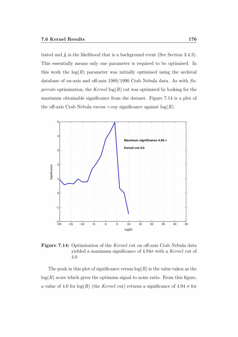
7.6 Kernel Results 176

tiated and fb is the likelihood that is a background event (See Section 3.4.3).

This essentially means only one parameter is required to be optimised. In

this work the log(R) parameter was initially optimised using the archival

database of on-axis and off-axis 1989/1990 Crab Nebula data. As with Su-

percuts optimisation, the Kernel log(R) cut was optimised by looking for the

maximum obtainable significance from the dataset. Figure 7.14 is a plot of

the off-axis Crab Nebula excess γ-ray significance against log(R).

−20 −15 −10 −5 0 5 10 15 20 25 30 35−2

−1

0

1

2

3

4

5

log(R)

Sig

nific

ance

Maximum significance 4.94 σ Kernel cut 4.0

Figure 7.14: Optimisation of the Kernel cut on off-axis Crab Nebula datayielded a maximum significance of 4.94σ with a Kernel cut of4.0

The peak in this plot of significance versus log(R) is the value taken as the

log(R) score which gives the optimum signal to noise ratio. From this figure,

a value of 4.0 for log(R) (the Kernel cut) returns a significance of 4.94 σ for

7.6 Kernel Results 177

Kernel analysis Significance ResultsSource Crab On-axis Crab Off-axis TeV J2032

Test data 10.75σ 3.74σ —–Independent data 11.14σ 3.21σ —–

All data —– —– 2.43σ

Table 7.9: Summary of significance results obtained using the Kernel anal-ysis technique.

the off-axis dataset of Crab Nebula data. When the technique is applied to

the on-axis data, the peak value of log(R) is also found to be 4.0 and returns

a maximum significance of 14.31 σ. When the technique is applied to the

TeV J2032+4130 dataset a reduction in significance of 27% (compared to

the value returned by standard Supercuts) is reported. Unfortunately these

significance values do not represent an improvement in the detected signal

over the original Supercuts analysis results or the energy-dependent cuts as

attempted in this work. This is possibly due to the fact that the Kernel

technique does not always perform well when applied to a dataset containing

a weak γ-ray signal, as it has a tendency to reject small events (Moriarty

et al., 1997). In addition to containing a weak signal, the source is also offset

from the centre of the field of view, which may also affect the effectiveness

of the Kernel analysis technique. Tables 7.9 and 7.10 provide a summary

of the significance and rate results after application of the Kernel analysis

technique. The results from the HEGRA position, using the various analysis

methods described here, returned, on average, a reduction in significance of

39% when compared to the value returned by Supercuts.

7.7 Energy Threshold and Flux Calculation 178

Kernel Analysis Rate ResultsSource Crab On-axis Crab Off-axis TeV J2032

Test data 0.63±0.06 0.31±0.10 —–Independent data 0.67±0.06 0.21±0.10 —–

All data —– —– 0.04±0.02

Table 7.10: Summary of the rate (γ min−1) values obtained using the Ker-nel analysis technique.

7.7 Energy Threshold and Flux Calculation

As already stated in Section 7.4.3, Figure 7.12 suggested an energy threshold

of ∼ 450 GeV. This value can be regarded as an estimate. For a more formal

calculation of the energy threshold of the imaging atmospheric Cherenkov

telescope, the collection area of the detector must be calculated first. The

collection area gives a clearer indication of the performance and efficiency of

the imaging atmospheric Cherenkov telescope at a given energy.

Collection area is calculated using the simulated γ-rays that fell randomly

over the area Ao5. Ao is chosen to be large enough to contain all triggering

events. (It is assumed that events outside Ao never trigger the camera).

The number of events that trigger the camera (located at the centre of Ao)

and pass analysis are recorded, as are the total number of simulated γ-rays

generated. The collection area is defined as:

A(E) = Ao

(No. of simulated gammas triggering at energy E

No. of simulated gammas at energy E

)(7.4)

The collection area is representative of the area over which Cherenkov events

trigger the telescope and is much larger than the physical dimensions of

5Ao = π(250m)2 and 250m is the impact radius or the distance between the showeraxis and the instrument. Also known as the impact parameter.

7.7 Energy Threshold and Flux Calculation 179

−1 −0.5 0 0.5 1 1.5 20

1

2

3

4

5

6

7

8

9

10

11x 10

4

log Energy (TeV)

Col

lect

ion

Are

a (m

2 )

Collection Area Distribution for Simulated Gamma rays

Figure 7.15: Collection area for γ-ray simulations generated for the1989/1990 camera configuration.

the telescope. Figure 7.15 illustrates collection area curve as a function of

energy. From this plot a collection area of ∼ 55 × 103 m2 is found. This

value compares favorably with the curve previously derived in Krennrich

et al. (2001) and Kildea (2002). For the collection area to be useful for more

than just investigating the sensitivity of the telescope to γ-rays of different

energies, i.e. to provide information regarding the response of the detector

to a given source, the collection area is convolved with the particular energy

spectrum of the source being observed (Kertzman & Sembroski, 1994). This

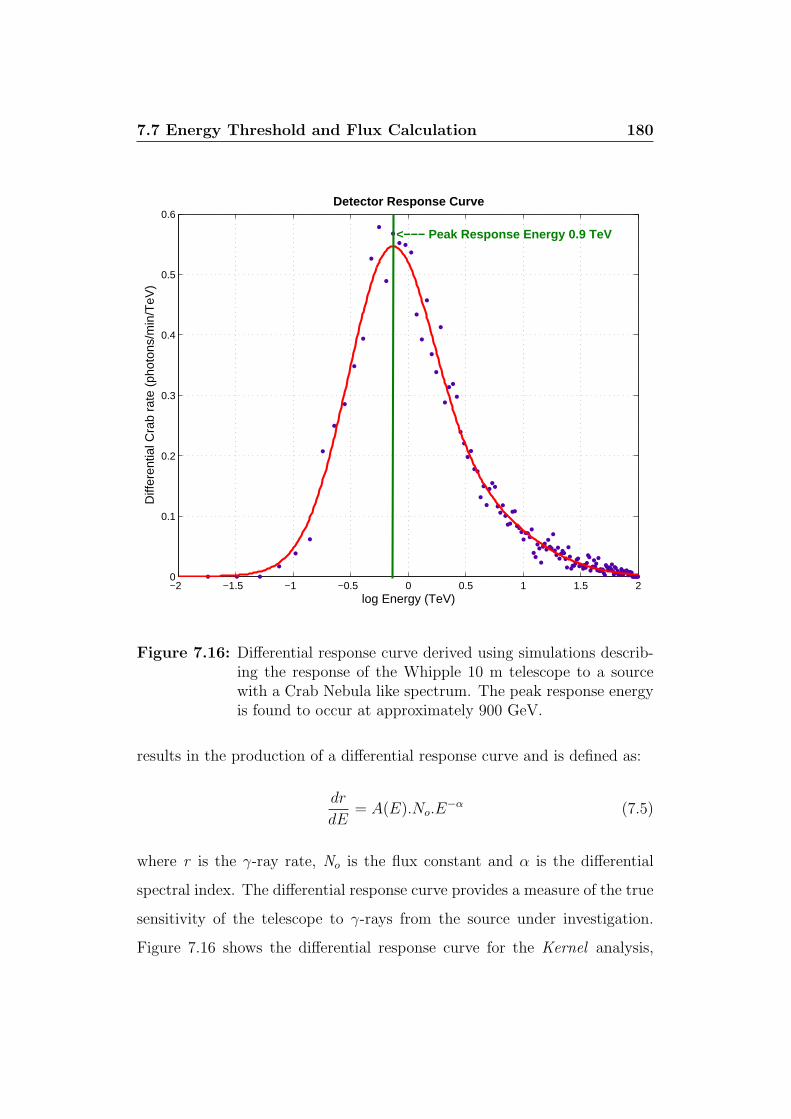
7.7 Energy Threshold and Flux Calculation 180

−2 −1.5 −1 −0.5 0 0.5 1 1.5 20

0.1

0.2

0.3

0.4

0.5

0.6

log Energy (TeV)

Diff

eren

tial C

rab

rate

(ph

oton

s/m

in/T

eV)

Detector Response Curve

<−−− Peak Response Energy 0.9 TeV

Figure 7.16: Differential response curve derived using simulations describ-ing the response of the Whipple 10 m telescope to a sourcewith a Crab Nebula like spectrum. The peak response energyis found to occur at approximately 900 GeV.

results in the production of a differential response curve and is defined as:

dr

dE= A(E).No.E

−α (7.5)

where r is the γ-ray rate, No is the flux constant and α is the differential

spectral index. The differential response curve provides a measure of the true

sensitivity of the telescope to γ-rays from the source under investigation.

Figure 7.16 shows the differential response curve for the Kernel analysis,

7.7 Energy Threshold and Flux Calculation 181

fitted with a two-term Gaussian distribution curve, and was obtained using

the differential spectrum of the Crab Nebula: (3.20 × 10−7 × (E/1 TeV)−2.49

m−2s−1TeV−1) taken from Hillas et al. (1998).

The peak position on the differential response curve is representative of

the instrument’s peak response energy. The peak response energy for an

on-axis Crab Nebula signal, as shown in Figure 7.16, occurs at 900 GeV and

compares well to the previous estimate (Section 7.4.3) and to measurements

taken when the 109 PMT camera was in operation. The peak response energy

for an off-axis Crab Nebula signal was found to be ∼ 1 TeV. The differen-

tial response curve can also be used to provide an accurate measurement of

the energy threshold of the instrument, however the method used to deter-

mine this value must be defined. Kertzman & Sembroski (1994) quote three

different definitions for energy threshold and emphasise the importance of

reporting which method was used to determine the energy threshold. The

three methods are

The maximum in the differential response curve.

The energy at which the differential response curve reaches one half its

maximum value.

The energy such that the integral of the differential response curve is

95% of the total rate.

For the work carried out in this project, the energy threshold of the detector

is defined as the energy at which the differential response curve reaches one

half its maximum value. This corresponds to a threshold energy of ∼ 480

GeV for on-axis Crab Nebula data and to ∼ 620 GeV for off-axis Crab Nebula

data. Again these values compare well to previous values quoted of energy

7.7 Energy Threshold and Flux Calculation 182

threshold of the Whipple 10 m telescope configured with the 109 PMT camera

(Reynolds et al., 1993; Hillas et al., 1998).

The differential response curve defined in Equation 7.5 can also be ex-

pressed as:dr

dE= Ao.R(E).N(E) (7.6)

where N(E) is the source spectrum and R(E) is the fraction of events trig-

gering the camera at energy E. The source spectrum, N(E) is defined as:

N(E) = No.E−α (7.7)

When the area under the differential response curve is integrated, it returns

the number of γ-ray events per unit time: Nγ/T i.e. the rate of γ-ray detec-

tion from the source under investigation. Equation 7.8 defines this relation-

ship: ∫ ∞

0

Ao.R(E).N(E) dE =Nγ

T(7.8)

Equation 7.8 can be expanded and rewritten as:

Ao.No

∫ ∞

0

R(E).E−α dE =Nγ

T(7.9)

Since the measured significance of the γ-ray signal from the off-axis database

of TeV J2032+4130 is not high enough to determine the spectral index, a

priori knowledge regarding the source’s γ-ray spectrum was assumed. Equa-

tion 7.9 can be rearranged to provide a means of calculating the differential

flux and hence the integral flux of the source being studied

No =Nγ

T.Ao

∫∞0

R(E).E−α dE(7.10)

7.7 Energy Threshold and Flux Calculation 183

The implication of Equation 7.10 is that the only required input to return a

value for the differential flux is the spectral index α. By using this technique

the differential flux of the Crab Nebula was calculated to be (3.4 ±0.2 ±0.2)

× 10−7 × (E/1 TeV)−2.49 m−2s−1TeV−1 which yields an integral flux of (2.3

±0.2 ±0.3) × 10−7 m−2s−1 above 1 TeV. The first uncertainty represents the

statistical uncertainties in the calculation and was obtained using knowledge

of the reported significance of the source and the reported flux values. The

second uncertainty represents the systematic uncertainties in the flux and

was obtained by combining the percent uncertainties on the spectral index

of the source and the percent uncertainties on R(E). It was found that the

systematic uncertainties were dominated by the uncertainties in the spectral

index. When the same approach is applied to simulations from an offset

source with a Crab-like spectrum, a differential flux of (3.0 ±0.6 ±0.3) × 10−7

× (E/1 TeV)−2.49 m−2s−1TeV−1 is found. This leads to an offset integral flux

of (2.0 ±0.4 ±0.2) × 10−7 m−2s−1. These flux values for an offset source are

encouraging as they are within the tolerance limits of the accepted values of

the differential (3.20 ±0.17 ±0.6) × 10−7 × (E/1 TeV)−2.49 m−2s−1TeV−1 and

integral flux (2.1 ±0.2 ±0.3) × 10−7 m−2s−1 of the Crab Nebula as reported

by Hillas et al. (1998) and thus provide confidence in the methodology used

to determine these flux values.

When the calculation is performed using simulations of an offset source

with a spectral index matching that of the HEGRA value (Aharonian et al.,

2005i) found after a spectral analysis of TeV J2032+4130, the differential flux

was found to be (1.2 ±0.4 ±0.4) × 10−8 × (E/1 TeV)−1.9 m−2s−1TeV−1. The

integral flux was determined to be (1.3 ±0.4 ±0.5) × 10−8 m−2s−1 above 1

TeV. This represents a value of 6.2% of the Crab Nebula flux and is consistent

7.7 Energy Threshold and Flux Calculation 184

with the value calculated by the HEGRA collaboration which lends strength

to the argument that TeV J2032+4130 is a steady source of TeV γ-rays. This

is an important result in the quest to the determine the nature of the TeV

emitter TeV J2032+4130 and will be discussed further in the next chapter.

Chapter 8

Discussion

8.1 Summary of Work

The work carried out in this thesis can be viewed as two separate entities.

In the early stages of the project, a twofold approach to try and improve

the optical performance of the 10 m class of imaging atmospheric Cherenkov

telescope was undertaken. The two approaches were designed and undertaken

to complement one another in the manner in which the optical improvement

would be carried out. One was an attempt to physically improve the optical

characteristics of the telescope by reducing the Point Spread Function (PSF)

to as small a value as possible, and the other would use this improved PSF

to computationally “sharpen” the recorded Cherenkov images to allow better

discrimination between γ-ray initiated EAS and hadronic showers.

As was noted in Chapter 5, the sharpening of the images was not suc-

cessful in improving the signal to noise ratio of the telescope. However the

semi-automated alignment system constructed in NUI, Galway was success-

ful and is in use aligning the telescopes of the new VERITAS array system

in Southern Arizona.

8.1 Summary of Work 186

Subsequent to this subproject the main objective of the project was un-

dertaken. This involved a detailed reanalysis an archived Cygnus dataset

that contained a “hot-spot” offset in the camera’s field of view in the region

of the HEGRA unidentified object TeV J2032+4130. The main objective

of this reanalysis was the determination of the integral flux of VHE γ-ray

photons from the source TeV J2032+4130. This was of particular interest

as recent results from Aharonian et al. (2005i) and Konopelko et al. (2007)

suggest that TeV J2032+4130 is a steady source of VHE γ-rays with integral

fluxes determined to be 5% and 8% of the Crab Nebula flux respectively.

These results are reported for data from 1999 to 2002 for HEGRA and from

2003 to 2005 for the VERITAS Whipple 10 m telescope data. However, Lang

et al. (2004) estimated, from the 1989/1990 dataset, the integral flux to be

12% of the Crab Nebula flux, thus suggesting possible source variability over

the timescale of initial observations to the most recent observations. Since

the detected off-axis signal contained in the Cygnus dataset was very weak,

it was not within the scope of this project to determine the TeV spectrum of

TeV J2032+4130.

In addition to determining the γ-ray flux from TeV J2032+4130, the

archival data was reanalysed using methods, that at the time of the original

observations, were not in use, such as two dimensional analysis and the Ker-

nel technique, with the aim of improving the statistical excess of the signal.

During this part of the project, and to facilitate the Kernel analysis pro-

cedure, a database of γ-ray simulations was generated after the creation of

the configuration file, as described in Chapter 6, to represent the 109 PMT

camera configuration.

These alternative analysis methods used here were a final attempt at

improving the detected γ-ray significance from TeV J2032+4130. As the

8.2 Flux Determination of TeV J2032+4130 187

Kernel technique was not fully developed at the time of the original analysis

of the Cygnus data, this effort was the first time such an analysis was carried

out on the offset VHE signal contained in the archived Cygnus dataset.

After applying a full analysis on the on-axis and off-axis Crab Nebula

data sets and on the Cygnus dataset using the alternative analysis methods

described in Chapter 6, no improvement in significance from any of the three

data sets was found.

8.2 Flux Determination of TeV J2032+4130

After deriving the effective collection area and the peak response energy

from the simulations database it was possible, with confidence in the γ-ray

simulations, to calculate the differential and integral flux values that appear

to confirm TeV J2032+4130 as a steady source of TeV γ-rays as indicated

by Aharonian et al. (2005i) and Konopelko et al. (2007). The method used

to carry out these calculations has been described in Section 7.7. As a test

of the validity of this method, the calculations to determine differential and

integral flux were first performed on the dataset of on-axis Crab Nebula data.

The resultant value was found to be within the tolerances of the accepted

integral flux value (Hillas et al., 1998).

The calculation was repeated on the off-axis Crab Nebula dataset and

again a value was returned that was within the tolerances of the accepted

integral flux value, confirming that the procedure could be carried out on off-

axis data. The procedure was then carried out on the dataset containing the

weak signal from TeV J2032+4130 and the integral flux value was calculated

to be (1.3 ±0.4 ±0.5) × 10−8 m−2s−1 above 1 TeV.

Assuming a spectral index of -1.9, the integrated flux value was found

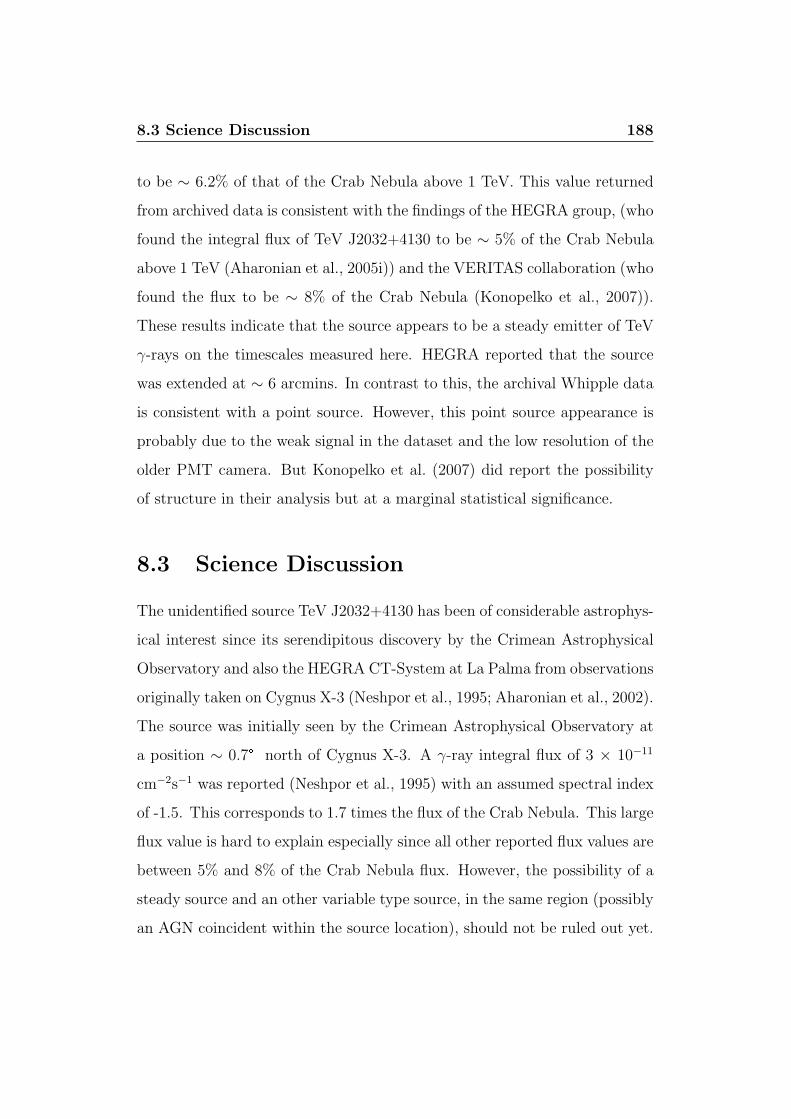
8.3 Science Discussion 188

to be ∼ 6.2% of that of the Crab Nebula above 1 TeV. This value returned

from archived data is consistent with the findings of the HEGRA group, (who

found the integral flux of TeV J2032+4130 to be ∼ 5% of the Crab Nebula

above 1 TeV (Aharonian et al., 2005i)) and the VERITAS collaboration (who

found the flux to be ∼ 8% of the Crab Nebula (Konopelko et al., 2007)).

These results indicate that the source appears to be a steady emitter of TeV

γ-rays on the timescales measured here. HEGRA reported that the source

was extended at ∼ 6 arcmins. In contrast to this, the archival Whipple data

is consistent with a point source. However, this point source appearance is

probably due to the weak signal in the dataset and the low resolution of the

older PMT camera. But Konopelko et al. (2007) did report the possibility

of structure in their analysis but at a marginal statistical significance.

8.3 Science Discussion

The unidentified source TeV J2032+4130 has been of considerable astrophys-

ical interest since its serendipitous discovery by the Crimean Astrophysical

Observatory and also the HEGRA CT-System at La Palma from observations

originally taken on Cygnus X-3 (Neshpor et al., 1995; Aharonian et al., 2002).

The source was initially seen by the Crimean Astrophysical Observatory at

a position ∼ 0.7° north of Cygnus X-3. A γ-ray integral flux of 3 × 10−11

cm−2s−1 was reported (Neshpor et al., 1995) with an assumed spectral index

of -1.5. This corresponds to 1.7 times the flux of the Crab Nebula. This large

flux value is hard to explain especially since all other reported flux values are

between 5% and 8% of the Crab Nebula flux. However, the possibility of a

steady source and an other variable type source, in the same region (possibly

an AGN coincident within the source location), should not be ruled out yet.

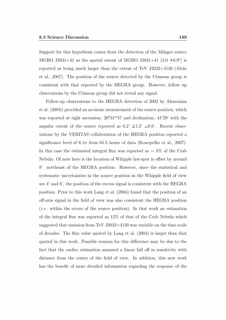
8.3 Science Discussion 189

Support for this hypothesis comes from the detection of the Milagro source

MGRO J2031+41 as the spatial extent of MGRO J2031+41 (3.0 ±0.9°) is

reported as being much larger than the extent of TeV J2032+4130 (Abdo

et al., 2007). The position of the source detected by the Crimean group is

consistent with that reported by the HEGRA group. However, follow up

observations by the Crimean group did not reveal any signal.

Follow-up observations to the HEGRA detection of 2002 by Aharonian

et al. (2005i) provided an accurate measurement of the source position, which

was reported at right ascension: 20h31m57 and declination: 41°29’ with the

angular extent of the source reported as 6.2’ ±1.2’ ±0.9’. Recent obser-

vations by the VERITAS collaboration of the HEGRA position reported a

significance level of 6.1σ from 65.5 hours of data (Konopelko et al., 2007).

In this case the estimated integral flux was reported as ∼ 8% of the Crab

Nebula. Of note here is the location of Whipple hot-spot is offset by around

9’ northeast of the HEGRA position. However, since the statistical and

systematic uncertainties in the source position in the Whipple field of view

are 4’ and 6’, the position of the excess signal is consistent with the HEGRA

position. Prior to this work Lang et al. (2004) found that the position of an

off-axis signal in the field of view was also consistent the HEGRA position

(i.e. within the errors of the source position). In that work an estimation

of the integral flux was reported as 12% of that of the Crab Nebula which

suggested that emission from TeV J2032+4130 was variable on the time scale

of decades. The flux value quoted by Lang et al. (2004) is larger than that

quoted in this work. Possible reasons for this difference may be due to the

fact that the earlier estimation assumed a linear fall off in sensitivity with

distance from the centre of the field of view. In addition, this new work

has the benefit of more detailed information regarding the response of the

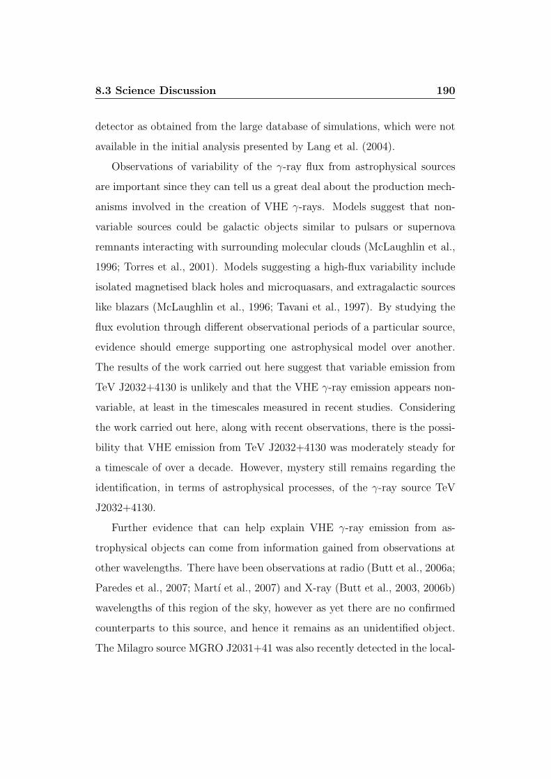
8.3 Science Discussion 190

detector as obtained from the large database of simulations, which were not

available in the initial analysis presented by Lang et al. (2004).

Observations of variability of the γ-ray flux from astrophysical sources

are important since they can tell us a great deal about the production mech-

anisms involved in the creation of VHE γ-rays. Models suggest that non-

variable sources could be galactic objects similar to pulsars or supernova

remnants interacting with surrounding molecular clouds (McLaughlin et al.,

1996; Torres et al., 2001). Models suggesting a high-flux variability include

isolated magnetised black holes and microquasars, and extragalactic sources

like blazars (McLaughlin et al., 1996; Tavani et al., 1997). By studying the

flux evolution through different observational periods of a particular source,

evidence should emerge supporting one astrophysical model over another.

The results of the work carried out here suggest that variable emission from

TeV J2032+4130 is unlikely and that the VHE γ-ray emission appears non-

variable, at least in the timescales measured in recent studies. Considering

the work carried out here, along with recent observations, there is the possi-

bility that VHE emission from TeV J2032+4130 was moderately steady for

a timescale of over a decade. However, mystery still remains regarding the

identification, in terms of astrophysical processes, of the γ-ray source TeV

J2032+4130.

Further evidence that can help explain VHE γ-ray emission from as-

trophysical objects can come from information gained from observations at

other wavelengths. There have been observations at radio (Butt et al., 2006a;

Paredes et al., 2007; Martı et al., 2007) and X-ray (Butt et al., 2003, 2006b)

wavelengths of this region of the sky, however as yet there are no confirmed

counterparts to this source, and hence it remains as an unidentified object.

The Milagro source MGRO J2031+41 was also recently detected in the local-

8.3 Science Discussion 191

ity of Cygnus (Abdo et al., 2007). However, at present all reports suggest TeV

J2032+4130 has no radio, optical or X-ray counterpart. Hence, this source

is currently considered unidentified and is regularly referred to as a “dark

accelerator”. Dark accelerators are a new class of VHE γ-ray source whose

characteristics include having no known counterpart at other wavelengths.

This indicates an absence of prominent leptonic synchrotron radiation lead-

ing to the possibility that these type of particle accelerators only accelerate

protons. At present these dark accelerators are not well understood and

further observations, at all wavelengths, are a priority that will hopefully

shed some light on these mysterious objects. The leading production models

related to dark accelerators are described here.

Association with Stellar Winds

The detection of γ-ray emission from dark accelerators using the model of

associated winds from massive hot stars in OB associations1 and Wolf-Rayet

(WR) type associations appears to be the most plausible explanation. At

least two of the current unidentified sources listed in Table 4.2, namely TeV

J2032+4130 (Aharonian et al., 2002) and HESS J1303-631 (Hartkopf et al.,

1999; Aharonian et al., 2005h), lie close to OB stellar associations. It has

been shown theoretically that particles can be accelerated up to energies of

hundreds of TeV due to the combination of effects of strong stellar winds

and supernova explosions (Bykov & Fleishman, 1992). In this scenario, the

stellar winds and supernova explosions at the core of the associations pro-

duce large scale shocks in which there are particles traveling at relativistic

velocities. If these particles were to collide with a dense medium, then, via

second-order Fermi acceleration (Fermi-II), significant γ-ray emission may be

1An OB association is a gravitationally unbound group of stars formed from the sameinterstellar cloud, containing a number of early spectral type (O and B) stars.

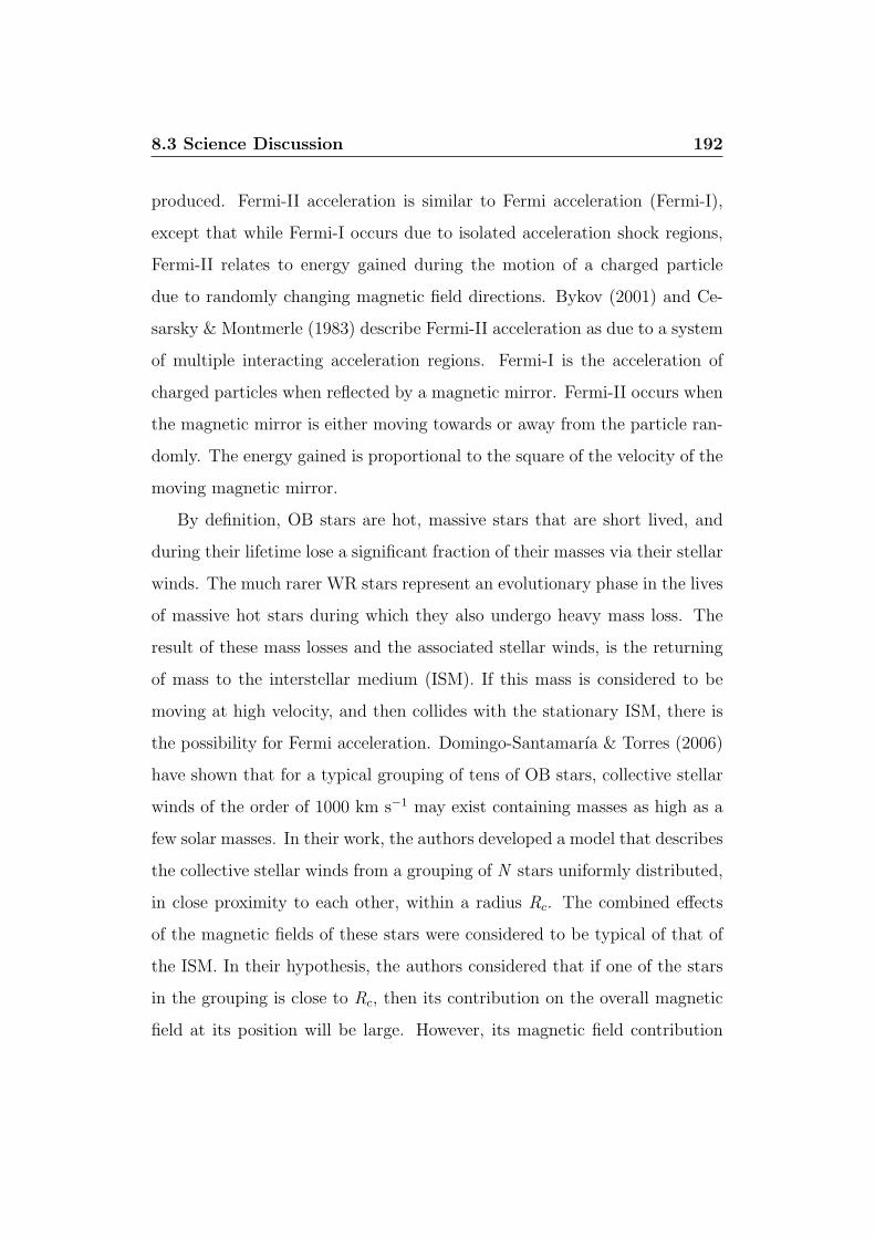
8.3 Science Discussion 192

produced. Fermi-II acceleration is similar to Fermi acceleration (Fermi-I),

except that while Fermi-I occurs due to isolated acceleration shock regions,

Fermi-II relates to energy gained during the motion of a charged particle

due to randomly changing magnetic field directions. Bykov (2001) and Ce-

sarsky & Montmerle (1983) describe Fermi-II acceleration as due to a system

of multiple interacting acceleration regions. Fermi-I is the acceleration of

charged particles when reflected by a magnetic mirror. Fermi-II occurs when

the magnetic mirror is either moving towards or away from the particle ran-

domly. The energy gained is proportional to the square of the velocity of the

moving magnetic mirror.

By definition, OB stars are hot, massive stars that are short lived, and

during their lifetime lose a significant fraction of their masses via their stellar

winds. The much rarer WR stars represent an evolutionary phase in the lives

of massive hot stars during which they also undergo heavy mass loss. The

result of these mass losses and the associated stellar winds, is the returning

of mass to the interstellar medium (ISM). If this mass is considered to be

moving at high velocity, and then collides with the stationary ISM, there is

the possibility for Fermi acceleration. Domingo-Santamarıa & Torres (2006)

have shown that for a typical grouping of tens of OB stars, collective stellar

winds of the order of 1000 km s−1 may exist containing masses as high as a

few solar masses. In their work, the authors developed a model that describes

the collective stellar winds from a grouping of N stars uniformly distributed,

in close proximity to each other, within a radius Rc. The combined effects

of the magnetic fields of these stars were considered to be typical of that of

the ISM. In their hypothesis, the authors considered that if one of the stars

in the grouping is close to Rc, then its contribution on the overall magnetic

field at its position will be large. However, its magnetic field contribution

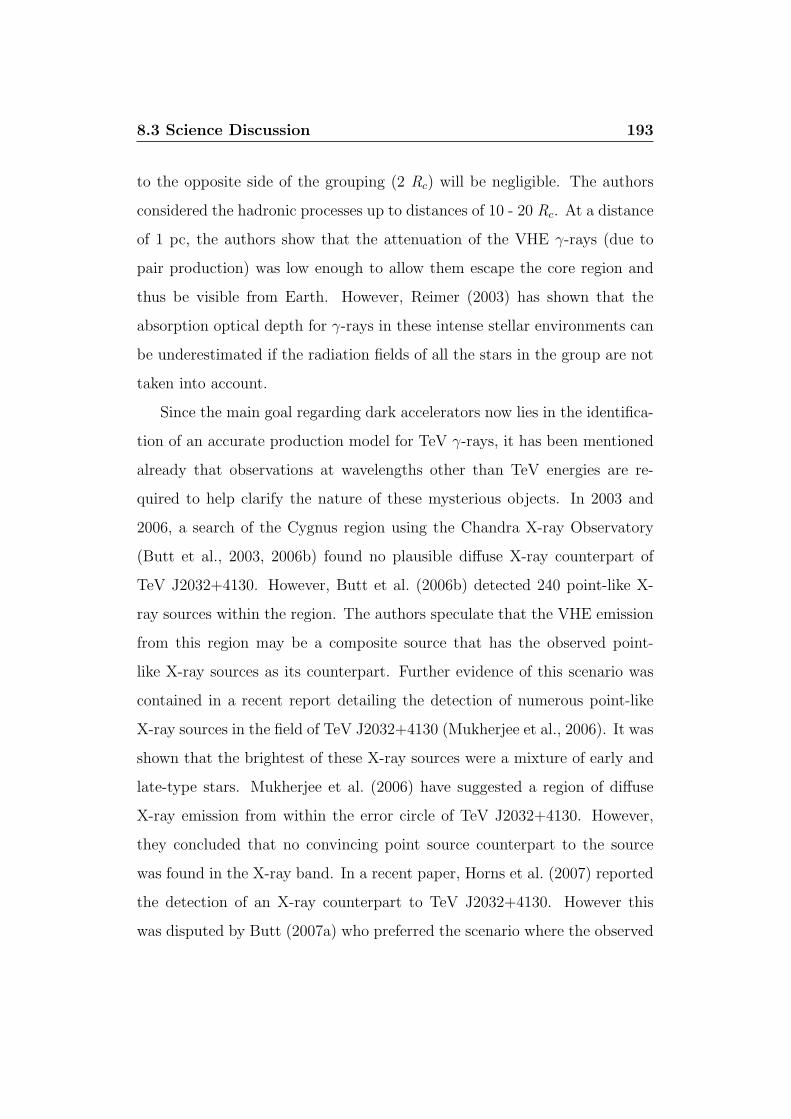
8.3 Science Discussion 193

to the opposite side of the grouping (2 Rc) will be negligible. The authors

considered the hadronic processes up to distances of 10 - 20 Rc. At a distance

of 1 pc, the authors show that the attenuation of the VHE γ-rays (due to

pair production) was low enough to allow them escape the core region and

thus be visible from Earth. However, Reimer (2003) has shown that the

absorption optical depth for γ-rays in these intense stellar environments can

be underestimated if the radiation fields of all the stars in the group are not

taken into account.

Since the main goal regarding dark accelerators now lies in the identifica-

tion of an accurate production model for TeV γ-rays, it has been mentioned

already that observations at wavelengths other than TeV energies are re-

quired to help clarify the nature of these mysterious objects. In 2003 and

2006, a search of the Cygnus region using the Chandra X-ray Observatory

(Butt et al., 2003, 2006b) found no plausible diffuse X-ray counterpart of

TeV J2032+4130. However, Butt et al. (2006b) detected 240 point-like X-

ray sources within the region. The authors speculate that the VHE emission

from this region may be a composite source that has the observed point-

like X-ray sources as its counterpart. Further evidence of this scenario was

contained in a recent report detailing the detection of numerous point-like

X-ray sources in the field of TeV J2032+4130 (Mukherjee et al., 2006). It was

shown that the brightest of these X-ray sources were a mixture of early and

late-type stars. Mukherjee et al. (2006) have suggested a region of diffuse

X-ray emission from within the error circle of TeV J2032+4130. However,

they concluded that no convincing point source counterpart to the source

was found in the X-ray band. In a recent paper, Horns et al. (2007) reported

the detection of an X-ray counterpart to TeV J2032+4130. However this

was disputed by Butt (2007a) who preferred the scenario where the observed

8.3 Science Discussion 194

X-ray emission was due to a population of faint X-ray sources that happen

by chance to be distributed at an angular size similar to TeV J2032+4130

and were previously reported (Butt et al., 2006b).

Butt et al. (2006b) state that at least 36 of the 240 detected X-ray sources

are massive stars and 2 are possible radio emitters. In their work, the authors

suggest that there is a critical distance from the core of the association where

VHE γ-ray emission, due to hadronic interactions in the shock front ∼ 1 pc

from the hot OB stars, outweighs absorption due to pair production. They

argue that this is the case for Cygnus OB2. Butt et al. (2003) have shown

that there is a sufficient grouping of catalogued OB stars that coincide with

TeV J2032+4130 ∼ 10 pc from the core of the association and they favour

the emission scenario described above. However further observations and

analysis are required to confirm this hypothesis.

Gamma-Ray Burst Remnants

The unidentified TeV source HESS J1303-631 was recently the subject of

a study that suggests the identification of the source as the remnant of a

Gamma-Ray Burst (GRB) that occurred in our Galaxy several tens of thou-

sands of years ago (Atoyan et al., 2006). GRBs are bursts of γ-rays coming

from seemingly random places in the sky, and at random times, that last

from milliseconds to many minutes. They are often followed by “afterglow”

emission at longer wavelengths (X-ray, UV, optical, IR, and radio) and at

the moment of occurrence they are the most luminous events known in the

universe. GRBs are currently detected about 2 to 3 times a week by orbiting

satellites. GRB models suggest that the intense, but brief, emission of en-

ergy may be caused by the core-collapse of a rapidly rotating high-mass star

into a singularity resulting in collimated emission. There is also a subclass

8.3 Science Discussion 195

of GRBs (“short” bursts) that appear to be due to other processes, possibly

the collision of two neutron stars orbiting in a binary system.

During a GRB, it is thought that there is a highly relativistic and ener-

getic outflow of matter forming a pair of opposite jets. The energy output

during the duration of the burst (≥ 2s) can be ∼ 6 × 1062 eV (Atoyan et al.,

2006). The relativistic shocks then accelerate particles in the plasma to rel-

ativistic energies. It is believed that the energy of these particles can be up

to ∼ 100 times higher than the accelerated particles produced in typical su-

pernova remnants (Berezinskii et al., 1990). If, from the estimated Galactic

GRB rate, there is between one and several GRBs of age ∼ 104 years in the

ISM at distances up to 10-20 kpc from Earth, then the associated shock of

accelerated multi-TeV particles would diffuse over distances of around 100 pc.

In this case, the detected VHE photons from GRB remnants should appear

as large centre-filled nebulae in the ISM. In their work Atoyan et al. (2006)

argue that one of the unidentified TeV sources, HESS J1303-631, can be

identified with the remnant of a GRB that happened in the Milky Way some

ten thousand years ago. Atoyan et al. (2006) predict that a main feature of a

GRB remnant is that a significant amount of the burst energy is eventually

transferred to high-energy protons. Relativistic electrons would only receive

a much smaller amount of energy during the point of non-relativistic evo-

lution of the GRB shell. According to Livio & Waxman (2000), the shock

from a GRB will become non-relativistic in less than one year and, by this

stage in their evolution, the associated magnetic fields would be around 0.1

G (Berger et al., 2004) and electrons will have cooled down via synchrotron

emission to a few GeV, thus providing an explanation for the lack of observed

synchrotron emission at high energies.

8.3 Science Discussion 196

Old SNR Associations

Another proposal put forward to explain VHE emission from dark accelera-

tors is the VHE γ-ray emission from old (> 105 years) supernova remnants

(Yamazaki et al., 2006). In their work, the authors find that the ratio of

the VHE flux to the X-ray or radio flux can be greater than 100, making

it very difficult to detect these sources at longer wavelengths. The authors

detail the possible encounter, and interaction, between an old SNR and a

giant molecular cloud. They suggest that if an old SNR interacts with a gi-

ant molecular cloud, VHE emission will occur via the Fermi-I process as the

SNR shock interacts with the dense giant molecular cloud. X-ray emission

will be negligible due to energy losses of the electrons over the lifetime of the

SNR. Two scenarios for particle acceleration are described. One where the

shock collides with the giant molecular cloud and one where the VHE emis-

sion comes from the giant molecular cloud being illuminated by accelerated

protons at the SNR shock. They noted that the maximum energy of accel-

erated electrons is much smaller, resulting in the generation of VHE γ-rays

being dominated by the acceleration of hadrons and their interaction within

the molecular cloud. The particles emit VHE γ-rays through π0 decay and

X-ray synchrotron emission from secondary electrons generated by charged

pions. However, the study showed that the shock created when a SNR older

than ∼ 5 × 104 years collides with a giant molecular cloud, particle accel-

eration in the shock is not efficient enough to produce VHE emission. Yet,

the high density of the giant molecular cloud can act as a target for the high

energy protons resulting in the production of pions. The possibility here is

that this type of hadronic acceleration could be the origin of VHE emission

from dark accelerators.

8.3 Science Discussion 197

Supernova-OB Associations

In a model put forward by Montmerle (1979), γ-ray emission from dark

accelerators may be due to a combination of the stellar winds from OB as-

sociated stars and a related SNR. Considering the size of the OB association

in Cygnus, it is possible that some of the oldest and more massive (10-20

M¯) member stars have already evolved into supernovae and that some of

the lower mass stars are still relatively close.

Microquasar emission

The models described above, or a combination of them, suggest steady emis-

sion of VHE γ-rays. Hence these models appear to be the most plausible

explanations for the emission of VHE γ-rays from dark accelerators, in partic-

ular TeV J2032+4130 given the results of this work and other recent studies.

There is, however, another suggestion that explains the VHE emission and

lack of detections at other energies. Aharonian et al. (2002) have suggested

an alternate accelerator, in the form of a microquasar, as a possible source

of variable γ-ray emission dark accelerators (Paredes et al., 2000). A micro-

quasar consists of a binary system in which a normal star orbits around, and

loses matter to, a nearby compact object. This object may be either a black

hole or a neutron star. The lost matter enters a fast-spinning accretion disk,

is heated to millions of degrees, and then either falls onto the compact object

or is ejected as a bipolar flow.

A possible scenario for VHE emission in this case involves a jet-driven

termination shock at the boundary, where a relativistic jet interacts with

the interstellar medium and where accelerated electrons produce synchrotron

emission and inverse-Compton emission (Aharonian & Atoyan, 1998a). In

fact the microquasar Cyg X-3 can be considered to be in the vicinity of TeV

8.3 Science Discussion 198

J2032-4130, at a distance of 70 pc, if it is at the same distance from Earth

(∼ 8.5 kpc). A recent report (Butt et al., 2006a), detailing a radio survey of

the TeV J2032+4130 region, has revealed a weak diffuse radio source within

the Whipple hotspot and, to a lesser degree the HEGRA position. The

radio source appears as a dual-lobed non-thermal source, however, a definite

determination on the nature of the source has not yet been made. It is also

not clear whether the source is Galactic or extragalactic. If it is Galactic,

there is a possibility that it is a microquasar. Thus it is still unclear if this

object is related to the VHE γ-ray emission observed from TeV J2032+4130.

Counterparts at Lower Energies

With regard to observations of TeV J2032+4130 in lower energy regimes,

there have been several tentative detections at radio and infrared frequencies

(Butt et al., 2006a; Paredes et al., 2007; Martı et al., 2007) of weak diffuse

sources in the region of sky consistent with the location of TeV J2032+4130.

Martı et al. (2007) have created a catalogue of 153 objects at the 49 cm

wavelength. Figure 8.1 shows a sky map of the radio signal from the Cygnus

region and a close-up of the dual-lobed radio source located within the Whip-

ple hot-spot as mentioned above. The detection of a weak non-thermal shell-

like supernova remnant type object was also reported (Butt et al., 2006a).

Results of these radio frequency observations appear to suggest the existence

of one or more supernova remnants or large-scale cluster shocks caused by

the association of the large amount of massive stars in Cyg OB2 (Butt et al.,

2007). Despite these detections at radio frequencies near TeV J2032+4130,

any physical association between them and TeV J2032+4130 has not yet

been determined with certainty.

If these sources of diffuse X-ray emission and radio frequency emission

8.3 Science Discussion 199

Figure 8.1: On the left a radio sky map of the Cygnus region. The blueoval is representative of the Whipple VHE γ-ray hot-spot andthe red circle represents the extended region containing theHEGRA emission. On the right is a close up of the dual-lobednon-thermal radio source located within the Whipple hotspot.2 represent the locations of the CHANDRA point-like X-raysources and I represent 2MASS infrared point sources. Figurecourtesy of Butt et al. (2006a).

are confirmed as being associated with TeV J2032+4130 by further observa-

tions, it should help to constrain the origin of TeV γ-ray emission from this

region of sky and assist in determining whether the emission is electronic or

hadronic in origin. Since there are a variety of nearby astrophysical sources

associated with Cygnus region, there is some credence in the theory that

the VHE γ-ray emission is due to a termination shock caused by supersonic

stellar winds breaking out into the inter stellar medium. In fact very recent

results from the HESS collaboration (Aharonian et al., 2007b) have detailed

the detection of VHE γ-ray emission from the powerful stellar association

Westerlund 2, in the southern sky, containing the Wolf-Rayet binary WR

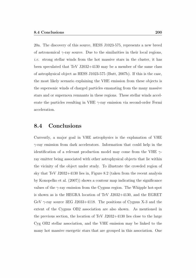
8.4 Conclusions 200

20a. The discovery of this source, HESS J1023-575, represents a new breed

of astronomical γ-ray source. Due to the similarities in their local regions,

i.e. strong stellar winds from the hot massive stars in the cluster, it has

been speculated that TeV J2032+4130 may be a member of the same class

of astrophysical object as HESS J1023-575 (Butt, 2007b). If this is the case,

the most likely scenario explaining the VHE emission from these objects is

the supersonic winds of charged particles emanating from the many massive

stars and or supernova remnants in these regions. These stellar winds accel-

erate the particles resulting in VHE γ-ray emission via second-order Fermi

acceleration.

8.4 Conclusions

Currently, a major goal in VHE astrophysics is the explanation of VHE

γ-ray emission from dark accelerators. Information that could help in the

identification of a relevant production model may come from the VHE γ-

ray emitter being associated with other astrophysical objects that lie within

the vicinity of the object under study. To illustrate the crowded region of

sky that TeV J2032+4130 lies in, Figure 8.2 (taken from the recent analysis

by Konopelko et al. (2007)) shows a contour map indicating the significance

values of the γ-ray emission from the Cygnus region. The Whipple hot-spot

is shown as is the HEGRA location of TeV J2032+4130, and the EGRET

GeV γ-ray source 3EG J2033+4118. The positions of Cygnus X-3 and the

extent of the Cygnus OB2 association are also shown. As mentioned in

the previous section, the location of TeV J2032+4130 lies close to the large

Cyg OB2 stellar association, and the VHE emission may be linked to the

many hot massive energetic stars that are grouped in this association. One

8.4 Conclusions 201

scenario, suggesting VHE emission due to the OB association, is hadronic

in nature (Aharonian et al., 2002). A second possibility explains the VHE

Figure 8.2: A VHE sky map of excess counts of the Cygnus region fromobservations taken with the Whipple 10 m imaging atmosphericCherenkov telescope. Overlayed are the positions of variousother astrophysical objects of note in this region. The centrecircle is the source location of TeV J2032+4130 as reportedby the HEGRA group. Also shown is the GeV γ-ray EGRETsource 3EG J2033+4118 as well as the extent of the CygnusOB association. Taken from Konopelko et al. (2007).

γ-ray emission as synchrotron and inverse Compton scattering in a jet-driven

termination shock from Cygnus X-3. There is also the possibility the jet could

originate from an as yet undetected microquasar or a class of high energy γ-

ray source. However, since the work carried out here suggests steady emission

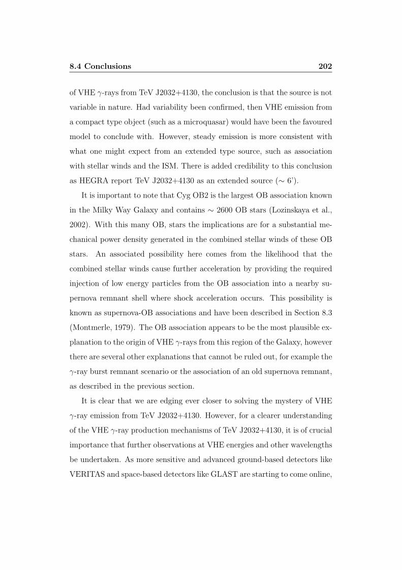
8.4 Conclusions 202

of VHE γ-rays from TeV J2032+4130, the conclusion is that the source is not

variable in nature. Had variability been confirmed, then VHE emission from

a compact type object (such as a microquasar) would have been the favoured

model to conclude with. However, steady emission is more consistent with

what one might expect from an extended type source, such as association

with stellar winds and the ISM. There is added credibility to this conclusion

as HEGRA report TeV J2032+4130 as an extended source (∼ 6’).

It is important to note that Cyg OB2 is the largest OB association known

in the Milky Way Galaxy and contains ∼ 2600 OB stars (Lozinskaya et al.,

2002). With this many OB, stars the implications are for a substantial me-

chanical power density generated in the combined stellar winds of these OB

stars. An associated possibility here comes from the likelihood that the

combined stellar winds cause further acceleration by providing the required

injection of low energy particles from the OB association into a nearby su-

pernova remnant shell where shock acceleration occurs. This possibility is

known as supernova-OB associations and have been described in Section 8.3

(Montmerle, 1979). The OB association appears to be the most plausible ex-

planation to the origin of VHE γ-rays from this region of the Galaxy, however

there are several other explanations that cannot be ruled out, for example the

γ-ray burst remnant scenario or the association of an old supernova remnant,

as described in the previous section.

It is clear that we are edging ever closer to solving the mystery of VHE

γ-ray emission from TeV J2032+4130. However, for a clearer understanding

of the VHE γ-ray production mechanisms of TeV J2032+4130, it is of crucial

importance that further observations at VHE energies and other wavelengths

be undertaken. As more sensitive and advanced ground-based detectors like

VERITAS and space-based detectors like GLAST are starting to come online,

8.5 Future Possibilities in Ground Based γ-ray Astronomy 203

it is only a matter of time before the issues surrounding unidentified and

dark accelerator candidates, like TeV J2032+4130, will be resolved. Future

observations with VERITAS and MAGIC will be critical in determining the

nature of TeV J2032+4130 as they will be able to accurately map the spatial

extent of the source.

8.5 Future Possibilities in Ground Based γ-

ray Astronomy

In the last few years the field of ground-based γ-ray astronomy has taken a

great leap forward with improved technologies and better funding. With the

HESS array fully functional in the southern hemisphere, and the VERITAS

array now online in the northern hemisphere, the entire sky can now be ob-

served with unprecedented sensitivity using similar instruments. The ever

expanding HESS catalogue is an example of the potential for discovery these

new Cherenkov arrays possess and provides great motivation for the contin-

ued development in the field. When GLAST comes online in early 2008, a

gap in the high energy spectrum will be closed as its upper energy threshold

will overlap with the lower energy thresholds of HESS and VERITAS. With

all this in mind, one must ask a question regarding the future of this field,

what next?

Generally, progress in astronomy can be seen in two distinct areas of activ-

ity. One involves the use of existing technologies on a much larger scale than

before. For example the scaling up from a single 10 m Cherenkov telescope

(Whipple 10 m) to an array of four 12 m Cherenkov telescopes (VERITAS

array) and the second phase of the HESS program, i.e. the addition of a

fifth large diameter Cherenkov telescope at the centre of the array. Another

8.5 Future Possibilities in Ground Based γ-ray Astronomy 204

example is the MAGIC collaboration’s addition of a second telescope 85 m

distance from the original, known as MAGIC II. The second area results from

technological breakthroughs and resulting improvements in sensitivity. For

example, optical astronomy took a huge leap forward due to the development

of CCD detectors, that subsequently replaced photographic plates resulting

in improved sensitivity and a convenient method of image analysis and data

storage. A significant breakthrough for ground-based γ-ray astronomy would

be the development of detectors with significant improvements in quantum

efficiency. However, progress in new technologies relating to VHE astronomy

have been slow to come about.

Currently progress in ground-based γ-ray astronomy is based on the

method of building more, and bigger versions of the early successful ex-

periments. For example the next generation extensive air shower detector,

HAWC (High Altitude Water Cherenkov) (Smith et al., 2007), is based on

the existing MILAGRO detector. To make advances in ground based γ-

ray astronomy, several areas must be looked at and then decide whether it is

practical or possible to move the development in a particular direction. For

example, desirable improvements include reducing the energy threshold of a

detector, increasing the field of view, increasing the collection area etc. In

relation to the work carried out in Chapter 6 of this project, it is clear that an

improved field of view would be of benefit when it comes to making serendip-

itous discoveries of hitherto undetected sources like TeV J2032+4130. Larger

fields of view may be obtained by using larger optical systems and cameras

with larger PMT cameras. An increase in collection area may be obtained

by using more imaging atmospheric Cherenkov telescopes, i.e. larger arrays.

A larger array of telescopes would improve sensitivity especially if the array

were larger than the Cherenkov light pool as it is seen from the ground.

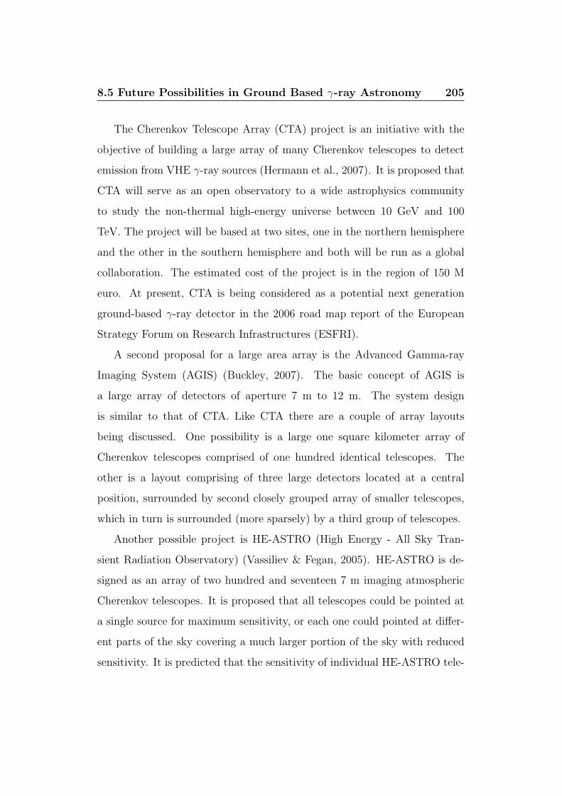
8.5 Future Possibilities in Ground Based γ-ray Astronomy 205

The Cherenkov Telescope Array (CTA) project is an initiative with the

objective of building a large array of many Cherenkov telescopes to detect

emission from VHE γ-ray sources (Hermann et al., 2007). It is proposed that

CTA will serve as an open observatory to a wide astrophysics community

to study the non-thermal high-energy universe between 10 GeV and 100

TeV. The project will be based at two sites, one in the northern hemisphere

and the other in the southern hemisphere and both will be run as a global

collaboration. The estimated cost of the project is in the region of 150 M

euro. At present, CTA is being considered as a potential next generation

ground-based γ-ray detector in the 2006 road map report of the European

Strategy Forum on Research Infrastructures (ESFRI).

A second proposal for a large area array is the Advanced Gamma-ray

Imaging System (AGIS) (Buckley, 2007). The basic concept of AGIS is

a large array of detectors of aperture 7 m to 12 m. The system design

is similar to that of CTA. Like CTA there are a couple of array layouts

being discussed. One possibility is a large one square kilometer array of

Cherenkov telescopes comprised of one hundred identical telescopes. The

other is a layout comprising of three large detectors located at a central

position, surrounded by second closely grouped array of smaller telescopes,

which in turn is surrounded (more sparsely) by a third group of telescopes.

Another possible project is HE-ASTRO (High Energy - All Sky Tran-

sient Radiation Observatory) (Vassiliev & Fegan, 2005). HE-ASTRO is de-

signed as an array of two hundred and seventeen 7 m imaging atmospheric

Cherenkov telescopes. It is proposed that all telescopes could be pointed at

a single source for maximum sensitivity, or each one could pointed at differ-

ent parts of the sky covering a much larger portion of the sky with reduced

sensitivity. It is predicted that the sensitivity of individual HE-ASTRO tele-

8.5 Future Possibilities in Ground Based γ-ray Astronomy 206

scopes, to observations of the Crab Nebula, would match that of VERITAS

(23σ/(hour)1/2) and when operated as a full array, its sensitivity would be

166σ/(hour)1/2, i.e. it would detect the Crab Nebula at 5σ in ∼ 3 seconds

(Swordy, 2007). The obvious and major drawback with this proposal is the

projected cost which is similar to that of CTA. To accomplish a project of

this nature, with such high costs, would require a wider international collab-

oration combined with the development and utilisation of new technologies.

The realisation of this would represent one of the biggest advances in this

field since its foundation.

Whatever the method used to advance the field of ground based γ-ray as-

tronomy, it is probable that larger arrays at higher altitudes (> 3000 m) with

lower energy thresholds will be developed. It is also probable that this field

of science will grow significantly in the coming years as collaborations grow

in size due to the large personnel requirements of such large experiments.

In conclusion, these proposed developments offer great potential for making

many new discoveries in the coming years and will surely lead to exciting

times ahead.

Appendix A

Hillas parameters

An image seen on the camera can be parameterised using information about

the size of the signal seen in each phototube. Suppose the ith PMT is given

coordinates xi, yi (in degrees) and contains a signal Si. The origin of the

coordinate system is in the centre of the array of PMTs. An ellipse is fitted

to the image and the Hillas parameters are calculated relative to the cen-

tre. By taking the moments of the image, the following parameters can be

determined.

〈x〉 =∑

sixi∑si

〈y〉 =∑

siyi∑si

〈x2〉 =∑

six2i∑

si〈y2〉 =

∑siy

2i∑

si

〈xy〉 =∑

sixiyi∑si

〈x3〉 =∑

six3i∑

si

〈y3〉 =∑

siy3i∑

si〈x2y〉 =

∑six

2i yi∑

si

〈xy2〉 =∑

sixiy2i∑

si

208

σx2 = 〈x2〉 − 〈x2〉

σy2 = 〈y2〉 − 〈y2〉

σxy = 〈xy〉 − 〈x〉 〈y〉

σx3 = 〈x3〉 − 3 〈x〉 〈x2〉+ 2 〈x〉3

σy3 = 〈y3〉 − 3 〈y〉 〈y2〉+ 2 〈y〉3

σx2y = 〈x2y〉 − 2 〈xy〉 〈x〉+ 2 〈x〉2 〈y〉 − 〈x2〉 〈y〉

σxy2 = 〈xy2〉 − 2 〈xy〉 〈y〉+ 2 〈x〉 〈y〉2 − 〈x〉 〈y2〉

By defining the following:

k = σy2 − σx2 l =√

k2 + 4σ2xy

m = 〈y2〉 − 〈x2〉 n =√

m2 + 4 〈xy〉2

u = 1 + kl

v = 2− u

209

the Hillas parameters are calculated as follows:

〈Size〉 =∑

si

〈Length〉2 =σx2+σy2+1

2

〈Width〉2 =σx2+σy2−1

2

〈Miss〉2 = u〈x〉2+v〈y〉22

− 2〈xy〉σxy

l

〈Azwidth〉2 = 〈x〉2+〈y〉2−n2

〈Dis tan ce〉2 = 〈x〉2 + 〈y〉2

〈Alpha〉 = sin−1(

〈Miss〉〈Dis tan ce〉

)

The calculation of the parameter asymmetry requires the angle, ψ, between

the x-axis and the major axis of the ellipse:

ψ = tan−1(

(k+l)〈y〉+2σxy〈x〉2σxy〈y〉−(k−l)〈x〉

),

p = σx3 cos3 ψ + 3σx2y sin ψ cos2 ψ + 3σxy2 cos ψ sin2 ψ + σy3 sin3 ψ,

〈Asymmetry〉3 = p〈Length〉

Appendix B

Publications List

Refereed Journal Publications:

A. Konopelko, & the VERITAS Collaboration including G.E. Kenny, 2007

Observations of the Unidentified TeV Gamma-Ray Source TeV

J2032+4130 with the Whipple Observatory 10 m Telescope. The

Astrophysical Journal, Volume 658, p. 1062.

J. Holder, & the VERITAS Collaboration including G.E. Kenny, 2006 VER-

ITAS: Status and Performance. Submitted to Proceedings of ”Science

with New Generation of High Energy Gamma-ray Experiments”, Elba.

J. Holder, & the VERITAS Collaboration including G.E. Kenny, 2006. The

First VERITAS Telescope. Astroparticle Physics, Volume 25, Issue 6, p.

391-401

J. S. Perkins, & the VERITAS Collaboration including G.E. Kenny, 2006.

211

TeV Gamma-Ray Observations of the Perseus and Abell 2029 Galaxy

Clusters. The Astrophysical Journal, Volume 644, Issue 1, pp. 148-154.

P. F. Rebillot, & the VERITAS Collaboration including G.E. Kenny, 2006.

Multiwavelength Observations of the Blazar Markarian 421 in 2002

December and 2003 January. The Astrophysical Journal, Volume 641,

Issue 2, pp. 740-751.

E. Linton, & the VERITAS Collaboration including G.E. Kenny, 2006. A

Search For Primordial Black Hole Evaporations using the Whipple

Gamma-ray Telescope. Journal of Cosmology and Astroparticle Physics,

Issue 01, pp. 013.

M. Schroedter, & the VERITAS Collaboration including G.E. Kenny, 2005.

A Very High Energy Gamma-Ray Spectrum of 1ES 2344+514. The

Astrophysical Journal, Volume 634, Issue 2, pp. 947-954.

M. Blazejowski, & the VERITAS Collaboration including G.E. Kenny, 2005.

A Multi-wavelength View of the TeV Blazar Markarian 421: Cor-

related Variability, Flaring, and Spectral Evolution. Astrophysical

Journal, 630 (1), 130-141.

M.K. Daniel, & the VERITAS Collaboration including G.E. Kenny, 2005.

Spectrum of Very High Energy Gamma-Rays from the blazar 1ES

1959+650 during Flaring Activity in 2002. Astrophysical Journal 621

181.

212

S.J. Fegan, & the VERITAS Collaboration including G.E. Kenny, 2005. A

Survey of Unidentified EGRET Sources at Very High Energies. As-

trophysical Journal 624 638.

A. Falcone, & the VERITAS Collaboration including G.E. Kenny, 2004.

A Search for TeV Gamma-Ray Emission form High-Peaked Flat

Spectrum Radio Quasars Using the Whipple Air-Cherenkov Tele-

scope. Astrophysical Journal 613 710.

D. Horan, & the VERITAS Collaboration including G.E. Kenny, 2004. Con-

straints on the very high energy emission from BL Lacertae objects.

Astrophysical Journal 603 (1): 51-61 Part 1.

K. Kosack, & the VERITAS Collaboration including G.E. Kenny, 2004.

TeV Gamma-Ray Observations of the Galactic Center. Astrophysical

Journal, 608 97.

S. Le Bohec, & the VERITAS Collaboration including G.E. Kenny, 2004.

Observation of M87 at 400GeV with the Whipple 10m telescope.

Astrophysical Journal, 610 (1), 156-160.

F. Krennrich, & the VERITAS Collaboration including G.E. Kenny, 2003.

VERITAS: the Very Energetic Imaging Telescope Array System.

New Astronomy Reviews. Vol 48, Issues 5-6, pp. 345-349.

213

Noncollaboration conference papers:

J. Toner, V. Acciari, A. Cesarini, G.G. Gillanders, D. Hanna, G. E. Kenny, J.

Kildea, A. McCann, M. McCutcheon, M.J. Lang, P. Reynolds, M. Schroedter,

A. Smith, J. E. Ward, T. Weekes, B. Zitzer. ICRC2007 Bias Alignment

of the VERITAS Telescopes. To be published in the proceedings of the

30th International Cosmic Ray Conference, Merida, Mexico.

G.E. Kenny, Gillanders, G.H., Lang, M.J., 2005. Point Spread Function

Deconvolution of an Atmospheric Cherenkov Telescope Proceedings

of the 28th International Cosmic Ray Conference, Pune, India

G.E. Kenny, November 2004. The Study of Very High Energy Gamma-

ray Emission from Astrophysical Objects. Poster presentation at the

Second IRCSET Annual Research Symposium in Dublin.

G.E. Kenny, November 2003. The Study of Very High Energy Gamma-

ray Emission from Astrophysical Objects using the Imaging Atmo-

spheric Cherenkov Technique. Poster presentation at the First IRCSET

Annual Research Symposium in Dublin.

G.E. Kenny, March 2003. An Overview of Gamma Ray Astronomy

and the Imaging Atmospheric Cherenkov Technique. Galway Physics

Society colloquium presentation.

VERITAS conference papers:

214

O. Celik, & the VERITAS Collaboration including G.E. Kenny, 2007. Ob-

servations of the Crab Nebula and Pulsar with VERITAS. To be

published in the proceedings of the 30th International Cosmic Ray Confer-

ence, Merida, Mexico.

P. Colin, & the VERITAS Collaboration including G.E. Kenny, 2007. Ob-

servation of the galaxy M87 with VERITAS. To be published in the

proceedings of the 30th International Cosmic Ray Conference, Merida, Mex-

ico.

P. Fortin, & the VERITAS Collaboration including G.E. Kenny, 2007. Ob-

servations of the high-frequency-peaked BL Lac object 1ES 1218+304

with VERITAS. To be published in the proceedings of the 30th Interna-

tional Cosmic Ray Conference, Merida, Mexico.

J. Grube, & the VERITAS Collaboration including G.E. Kenny, 2007. Ob-

servations of the Crab Nebula with the Whipple 10 m Telescope.

To be published in the proceedings of the 30th International Cosmic Ray

Conference, Merida, Mexico.

D. Horan, & the VERITAS Collaboration including G.E. Kenny, 2007. Ob-

servations of Gamma-ray Bursts with VERITAS and Whipple. To

be published in the proceedings of the 30th International Cosmic Ray Con-

ference, Merida, Mexico.

T. B. Humensky, & the VERITAS Collaboration including G.E. Kenny, 2007.

215

Observation of the Supernova Remnant IC 443 with VERITAS. To

be published in the proceedings of the 30th International Cosmic Ray Con-

ference, Merida, Mexico.

D. B. Kieda, & the VERITAS Collaboration including G.E. Kenny, 2007.

A VERITAS Search for VHE -Ray Point Sources Near Selected

MILAGRO Target Regions. To be published in the proceedings of the

30th International Cosmic Ray Conference, Merida, Mexico.

A. Konopelko, & the VERITAS Collaboration including G.E. Kenny, 2007.

Observations of Pulsar Wind Nebulae with the VERITAS Array

of Imaging Atmospheric Cherenkov Telescopes. To be published in

the proceedings of the 30th International Cosmic Ray Conference, Merida,

Mexico.

H. Krawczynski, & the VERITAS Collaboration including G.E. Kenny, 2007.

Blazar Observations with VERITAS. To be published in the proceed-

ings of the 30th International Cosmic Ray Conference, Merida, Mexico.

G. Maier, & the VERITAS Collaboration including G.E. Kenny, 2007. Ob-

servation of the binary system LS I +61 303 in Very-High Energy

Gamma-Rays with VERITAS. To be published in the proceedings of the

30th International Cosmic Ray Conference, Merida, Mexico.

G. Maier, & the VERITAS Collaboration including G.E. Kenny, 2007. VER-

ITAS: Status and Latest Results. To be published in the proceedings of

the 30th International Cosmic Ray Conference, Merida, Mexico.

216

A. Smith, & the VERITAS Collaboration including G.E. Kenny, 2007. TeV

and X-ray Monitoring of LS I +61 303With VERITAS, Swift, and

RXTE. To be published in the proceedings of the 30th International Cosmic

Ray Conference, Merida, Mexico.

D. Steele, & the VERITAS Collaboration including G.E. Kenny, 2007. Re-

sults from the Blazar Monitoring Campaign at the Whipple 10m

Gamma-ray Telescope. To be published in the proceedings of the 30th

International Cosmic Ray Conference, Merida, Mexico.

P. Cogan, & the VERITAS Collaboration including G.E. Kenny, 2007. Ob-

servations of 1ES 0647+250 and 1ES 0806+524 with VERITAS.

To be published in the proceedings of the 30th International Cosmic Ray

Conference, Merida, Mexico.

P. Cogan, & the VERITAS Collaboration including G.E. Kenny, 2007. Anal-

ysis of Flash ADC Data With VERITAS. To be published in the pro-

ceedings of the 30th International Cosmic Ray Conference, Merida, Mexico.

P. Cogan, & the VERITAS Collaboration including G.E. Kenny, 2007. VE-

GAS, the VERITAS Gamma-ray Analysis Suite. To be published in

the proceedings of the 30th International Cosmic Ray Conference, Merida,

Mexico.

M. K. Daniel, & the VERITAS Collaboration including G.E. Kenny, 2007.

The VERITAS standard data analysis. To be published in the proceed-

217

ings of the 30th International Cosmic Ray Conference, Merida, Mexico.

M. K. Daniel, & the VERITAS Collaboration including G.E. Kenny, 2007.

Application of radiosonde data to VERITAS simulations. To be pub-

lished in the proceedings of the 30th International Cosmic Ray Conference,

Merida, Mexico.

S. J. Fegan, & the VERITAS Collaboration including G.E. Kenny, 2007.

Observations of Mrk 421 and Mrk 501 in Spring 2006 with VER-

ITAS. To be published in the proceedings of the 30th International Cosmic

Ray Conference, Merida, Mexico.

D. Hanna, & the VERITAS Collaboration including G.E. Kenny, 2007. Cal-

ibration Techniques for VERITAS. To be published in the proceedings

of the 30th International Cosmic Ray Conference, Merida, Mexico.

E. Hays, & the VERITAS Collaboration including G.E. Kenny, 2007. VER-

ITAS Data Acquisition. To be published in the proceedings of the 30th

International Cosmic Ray Conference, Merida, Mexico.

C.M.Hui, & the VERITAS Collaboration including G.E. Kenny, 2007. Laser

Atmospheric Studies with VERITAS. To be published in the proceed-

ings of the 30th International Cosmic Ray Conference, Merida, Mexico.

M.P. Kertzman, & the VERITAS Collaboration including G.E. Kenny, 2007.

The Whipple Strip Sky Survey. To be published in the proceedings of

the 30th International Cosmic Ray Conference, Merida, Mexico.

218

G. Maier, & the VERITAS Collaboration including G.E. Kenny, 2007. Monte

Carlo studies of the VERITAS array of Cherenkov telescopes. To

be published in the proceedings of the 30th International Cosmic Ray Con-

ference, Merida, Mexico.

T. Nagai, & the VERITAS Collaboration including G.E. Kenny, 2007. Focal

Plane Instrumentation of VERITAS. To be published in the proceed-

ings of the 30th International Cosmic Ray Conference, Merida, Mexico.

A. J. Syson, & the VERITAS Collaboration including G.E. Kenny, 2007.

A Probability Density Method for VHE Gamma-Ray Source Anal-

ysis. To be published in the proceedings of the 30th International Cosmic

Ray Conference, Merida, Mexico.

A. Weinstein, & the VERITAS Collaboration including G.E. Kenny, 2007.

The VERITAS Trigger System. To be published in the proceedings of

the 30th International Cosmic Ray Conference, Merida, Mexico.

S. A. Wissel, & the VERITAS Collaboration including G.E. Kenny, 2007.

Studies of Direct Cherenkov Emission with VERITAS. To be pub-

lished in the proceedings of the 30th International Cosmic Ray Conference,

Merida, Mexico.

J. Holder, & the VERITAS Collaboration including Kenny, G.E. 2005. In-

troduction to VERITAS. Proceedings of the 28th International Cosmic

Ray Conference, Pune, India, 2005.

219

P. Cogan, & the VERITAS Collaboration including Kenny, G.E. 2005. Tele-

scope 1 observations of AGN. Proceedings of the 28th International Cos-

mic Ray Conference, Pune, India, 2005.

G. Maier, & the VERITAS Collaboration including Kenny, G.E. 2005. Monte

Carlo results for Telescope 1. Proceedings of the 28th International Cos-

mic Ray Conference, Pune, India, 2005.

B. Humensky, & the VERITAS Collaboration including Kenny, G.E. 2005.

Muon calibration of Telescope 1. Proceedings of the 28th International

Cosmic Ray Conference, Pune, India, 2005.

J. Hall, & the VERITAS Collaboration including Kenny, G.E. 2005. Obser-

vations of local galaxies. Proceedings of the 28th International Cosmic

Ray Conference, Pune, India, 2005.

J. Holder, & the VERITAS Collaboration including Kenny, G.E. 2005. Ex-

ploiting VERITAS’ timing information. Proceedings of the 28th Inter-

national Cosmic Ray Conference, Pune, India, 2005.

J. Perkins, & the VERITAS Collaboration including Kenny, G.E. 2005. 10m

Observations of Perseus Cluster. Proceedings of the 28th International

Cosmic Ray Conference, Pune, India, 2005.

R. Atkins, & the VERITAS Collaboration including Kenny, G.E. 2005. 10m

Observations of the Cygnus Arm. Proceedings of the 28th International

220

Cosmic Ray Conference, Pune, India, 2005.

J. Grube, & the VERITAS Collaboration including Kenny, G.E. 2005. Spec-

tral Monitoring of Mrk-421. Proceedings of the 28th International Cos-

mic Ray Conference, Pune, India, 2005.

J. Holder, & the VERITAS Collaboration including Kenny, G.E. 2005. Sta-

tus and performance of the First VERITAS Telescope. Proceedings

of the 28th International Cosmic Ray Conference, Pune, India, 2005.

R. Rebillot, & the VERITAS Collaboration including Kenny, G.E. 2005.

Intensive Multiwavelength Observations of the Blazar Mrk421 in

December 2002 and January 2003. Proceedings of the 28th International

Cosmic Ray Conference, Pune, India, 2005.

J. Kildea, & the VERITAS Collaboration 2003. A Search for Pulsed

TeV Gamma-Ray Emission from the Crab Pulsar using the Whip-

ple High Resolution GRANITE III Camera. Proceedings of the 28th

International Cosmic Ray Conference, Tsukuba, pp. 2377-2380.

T.A. Hall, & the VERITAS Collaboration including Kenny, G.E. 2003. Very

High Energy Observations of PSR B1823-13. Proceedings of the 28th

International Cosmic Ray Conference, Tsukuba, pp. 2497-2500.

K. Kosack, & the VERITAS Collaboration including Kenny, G.E. 2003. TeV

Observations of the Galactic Center. Proceedings of the 28th Interna-

tional Cosmic Ray Conference, Tsukuba, pp. 2513-2516.

221

S. Le Bohec, & the VERITAS Collaboration including Kenny, G.E. 2003.

Search for a WIMP annihilation signature in the core of the glob-

ular cluster M15. Proceedings of the 28th International Cosmic Ray Con-

ference, Tsukuba, pp. 2521-2524.

G. Walker, & the VERITAS Collaboration including Kenny, G.E. 2003.

Whipple Telescope Observations of Potential TeV Gamma-Ray Sources

Found by the Tibet Air Shower Array. Proceedings of the 28th Inter-

national Cosmic Ray Conference, Tsukuba, pp. 2563-2566.

D. Horan, & the VERITAS Collaboration including Kenny, G.E. 2003. VHE

Observations of BL Lacertae Objects: 1995-2000. Proceedings of the

28th International Cosmic Ray Conference, Tsukuba, pp. 2567-2570.

I. de la Calle-Perez, & the VERITAS Collaboration including Kenny, G.E.

2003. Search for Very High Energy Gamma Rays from an X-ray

Selected Blazar sample. Proceedings of the 28th International Cosmic

Ray Conference, Tsukuba, pp. 2571-2574.

A. Falcone, & the VERITAS Collaboration including Kenny, G.E. 2003.

Search for TeV Emission at the Location of Milagro Sky Survey

Hot Spot Using the Whipple Gamma-Ray Telescope. Proceedings of

the 28th International Cosmic Ray Conference, Tsukuba, pp. 2579-2582.

P.F. Rebillot, & the VERITAS Collaboration including Kenny, G.E. 2003.

Intensive TeV Gamma-Ray and X-Ray Observations of the Blazar

222

Mrk 421 in December 2002 and January 2003. Proceedings of the 28th

International Cosmic Ray Conference, Tsukuba, pp. 2599-2602.

F. Krennrich, & the VERITAS Collaboration including Kenny, G.E. 2003.

Hourly Spectral Variability of Mrk 421. Proceedings of the 28th Inter-

national Cosmic Ray Conference, Tsukuba, pp. 2603-2606.

J. Holder, & the VERITAS Collaboration including Kenny, G.E. 2003. Whip-

ple observations of 1ES1959+650: an Update. Proceedings of the 28th

International Cosmic Ray Conference, Tsukuba, pp. 2619-2622.

S. LeBohec, & the VERITAS Collaboration including Kenny, G.E. 2003.

Observation of M87 with the Whipple 10m telescope. Proceedings of

the 28th International Cosmic Ray Conference, Tsukuba, pp. 2627-2630.

T. Nagai, & the VERITAS Collaboration including Kenny, G.E. 2003. Ob-

servations of Starburst Galaxies. Proceedings of the 28th International

Cosmic Ray Conference, Tsukuba, pp. 2635-2638.

D. Horan, & the VERITAS Collaboration including Kenny, G.E. 2003. Ob-

servations of H1426+428 from 1999 to 2002 with The Whipple

Observatory 10 m Telescope. Proceedings of the 28th International Cos-

mic Ray Conference, Tsukuba, pp. 2647-2650.

V.V. Vassiliev, & the VERITAS Collaboration including Kenny, G.E. 2003.

Search for TeV annihilation radiation from supersymmetric dark

matter in nearby galaxies. Proceedings of the 28th International Cosmic

223

Ray Conference, Tsukuba, pp. 2679-2682

S.P. Wakely, & the VERITAS Collaboration including Kenny, G.E. 2003.

The VERITAS Prototype. Proceedings of the 28th International Cosmic

Ray Conference, Tsukuba, pp. 2803-2806.

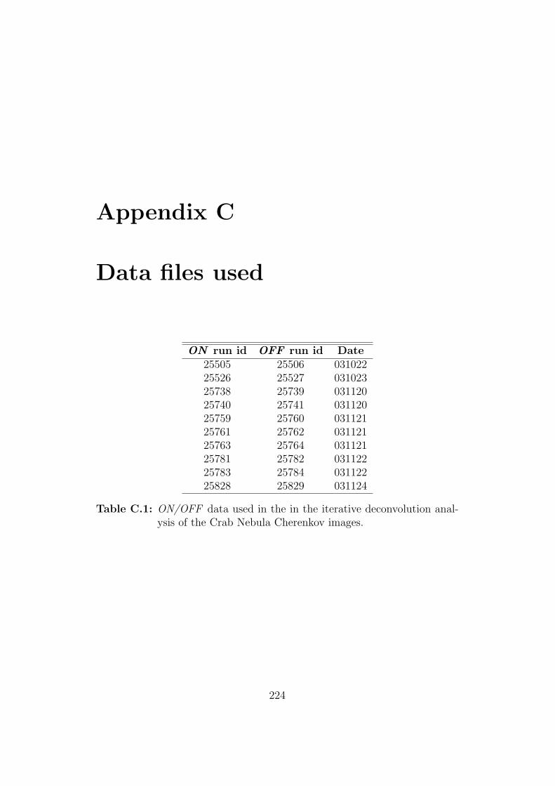
Appendix C

Data files used

ON run id OFF run id Date25505 25506 03102225526 25527 03102325738 25739 03112025740 25741 03112025759 25760 03112125761 25762 03112125763 25764 03112125781 25782 03112225783 25784 03112225828 25829 031124

Table C.1: ON/OFF data used in the in the iterative deconvolution anal-ysis of the Crab Nebula Cherenkov images.

224

ON run id OFF run id Datecr5117 cr5116 901015cr5118 cr5119 901015cr5148 cr5149 901016cr5150 cr5151 901016cr5152 cr5153 901016cr5229 cr5230 901021cr5231 cr5232 901021cr5255 cr5256 901022cr5257 cr5258 901022cr5259 cr5260 901022cr5261 cr5262 901022cr5281 cr5282 901023cr5283 cr5284 901023cr5285 cr5286 901023cr5287 cr5288 901023cr5311 cr5312 901024cr5314 cr5315 901024cr5336 cr5335 901025cr5339 cr5338 901025cr5351 cr5352 901026cr5353 cr5354 901026cr5355 cr5356 901026cr5389 cr5388 901028cr5397 cr5396 901029cr5399 cr5398 901029cr5820 cr5821 901219cr5827 cr5828 901219cr5850 cr5851 901220cr5852 cr5853 901220cr5854 cr5855 901220cr5939 cr5940 910113cr5941 cr5942 910113cr6006 cr6007 910118cr6008 cr6009 910118cr6028 cr6029 910119cr6030 cr6031 910119cr6032 cr6033 910119cr6034 cr6035 910119

Table C.2: ON/OFF on-axis Crab Nebula data files.

225

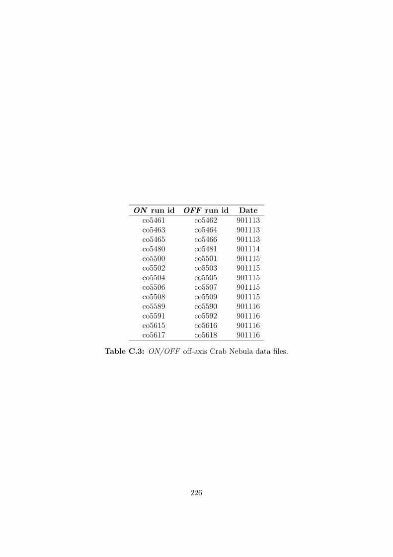
ON run id OFF run id Dateco5461 co5462 901113co5463 co5464 901113co5465 co5466 901113co5480 co5481 901114co5500 co5501 901115co5502 co5503 901115co5504 co5505 901115co5506 co5507 901115co5508 co5509 901115co5589 co5590 901116co5591 co5592 901116co5615 co5616 901116co5617 co5618 901116

Table C.3: ON/OFF off-axis Crab Nebula data files.

226

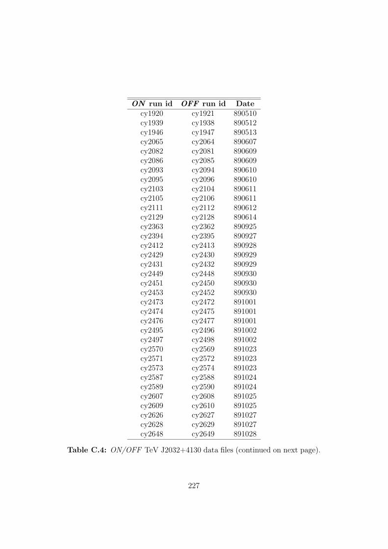
ON run id OFF run id Datecy1920 cy1921 890510cy1939 cy1938 890512cy1946 cy1947 890513cy2065 cy2064 890607cy2082 cy2081 890609cy2086 cy2085 890609cy2093 cy2094 890610cy2095 cy2096 890610cy2103 cy2104 890611cy2105 cy2106 890611cy2111 cy2112 890612cy2129 cy2128 890614cy2363 cy2362 890925cy2394 cy2395 890927cy2412 cy2413 890928cy2429 cy2430 890929cy2431 cy2432 890929cy2449 cy2448 890930cy2451 cy2450 890930cy2453 cy2452 890930cy2473 cy2472 891001cy2474 cy2475 891001cy2476 cy2477 891001cy2495 cy2496 891002cy2497 cy2498 891002cy2570 cy2569 891023cy2571 cy2572 891023cy2573 cy2574 891023cy2587 cy2588 891024cy2589 cy2590 891024cy2607 cy2608 891025cy2609 cy2610 891025cy2626 cy2627 891027cy2628 cy2629 891027cy2648 cy2649 891028

Table C.4: ON/OFF TeV J2032+4130 data files (continued on next page).

227

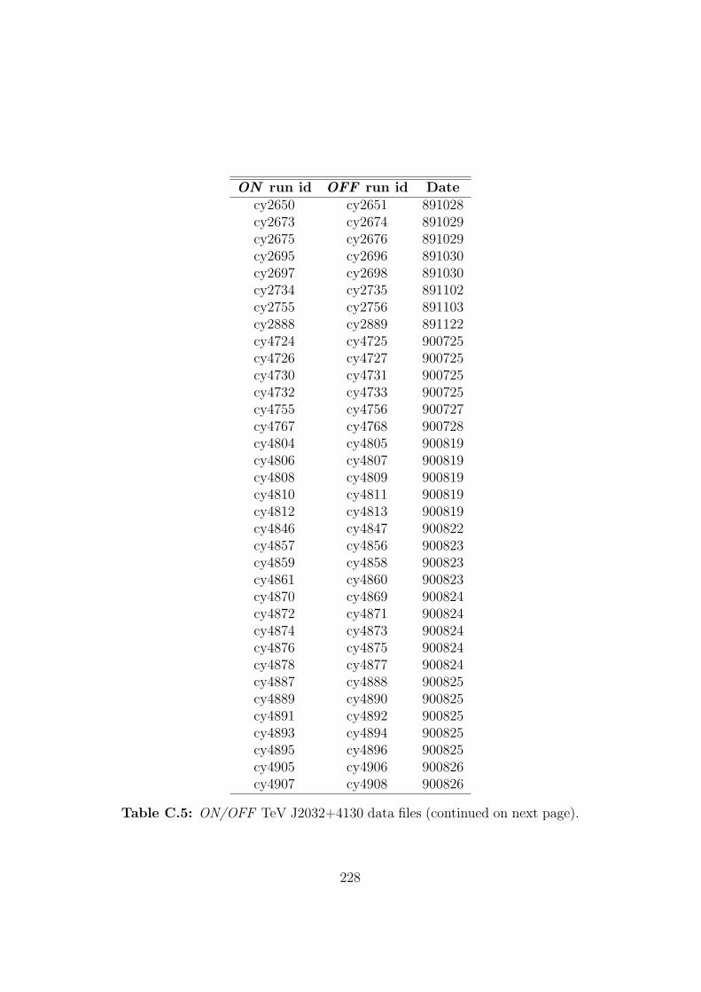
ON run id OFF run id Datecy2650 cy2651 891028cy2673 cy2674 891029cy2675 cy2676 891029cy2695 cy2696 891030cy2697 cy2698 891030cy2734 cy2735 891102cy2755 cy2756 891103cy2888 cy2889 891122cy4724 cy4725 900725cy4726 cy4727 900725cy4730 cy4731 900725cy4732 cy4733 900725cy4755 cy4756 900727cy4767 cy4768 900728cy4804 cy4805 900819cy4806 cy4807 900819cy4808 cy4809 900819cy4810 cy4811 900819cy4812 cy4813 900819cy4846 cy4847 900822cy4857 cy4856 900823cy4859 cy4858 900823cy4861 cy4860 900823cy4870 cy4869 900824cy4872 cy4871 900824cy4874 cy4873 900824cy4876 cy4875 900824cy4878 cy4877 900824cy4887 cy4888 900825cy4889 cy4890 900825cy4891 cy4892 900825cy4893 cy4894 900825cy4895 cy4896 900825cy4905 cy4906 900826cy4907 cy4908 900826

Table C.5: ON/OFF TeV J2032+4130 data files (continued on next page).

228

ON run id OFF run id Datecy4909 cy4910 900826cy4911 cy4912 900826cy4924 cy4923 900911cy4926 cy4925 900911cy5026 cy5027 901010cy5029 cy5028 901010cy5054 cy5055 901013cy5076 cy5077 901014cy5101 cy5102 901015cy5128 cy5127 901016cy5131 cy5132 901016cy5212 cy5211 901021cy5213 cy5214 901021

Table C.6: ON/OFF TeV J2032+4130 data files.

229

Bibliography

1 Abdo, A. A., et al. 2007, Astrophys. J. Lett., 664, L91

2 Abraham, J., et al. 2007, Science, 318, 938

3 Aharonian, F., et al. 2001, Astronomy and Astrophysics, 370, 112

4 Aharonian, F., et al. 2002, Astronomy and Astrophysics, 393, L37

5 Aharonian, F., et al. 2003, Astronomy and Astrophysics, 403, L1

6 Aharonian, F., et al. 2004, Astronomy and Astrophysics, 425, L13

7 Aharonian, F., et al. 2005a, Science, 307, 1938

8 Aharonian, F., et al. 2005b, Astronomy and Astrophysics, 437, L7

9 Aharonian, F., et al. 2005c, Astronomy and Astrophysics, 435, L17

10 Aharonian, F., et al. 2005d, Astronomy and Astrophysics, 442, 1

11 Aharonian, F., et al. 2005e, Science, 309, 746

12 Aharonian, F., et al. 2005f, Astronomy and Astrophysics, 436, L17

13 Aharonian, F., et al. 2005g, Astronomy and Astrophysics, 432, L9

14 Aharonian, F., et al. 2005h, Astronomy and Astrophysics, 439, 1013

15 Aharonian, F., et al. 2005i, Astronomy and Astrophysics, 431, 197

16 Aharonian, F., et al. 2005j, Astronomy and Astrophysics, 437, 135

17 Aharonian, F., et al. 2006a, Nature, 440, 1018

18 Aharonian, F., et al. 2006b, Astronomy and Astrophysics, 456, 245

19 Aharonian, F., et al. 2006c, Astronomy and Astrophysics, 448, L19

230

20 Aharonian, F., et al. 2006d, Astronomy and Astrophysics, 448, L43

21 Aharonian, F., et al. 2006e, Phys. Rev. Lett., 97, 221102

22 Aharonian, F., et al. 2006f, Astrophys. J., 636, 777

23 Aharonian, F., et al. 2007a, Astronomy and Astrophysics, 472, 489

24 Aharonian, F., et al. 2007b, Astronomy and Astrophysics, 467, 1075

25 Aharonian, F., Akhperjanian, A. G., Bazer-Bachi, A. R., & et al. 2006g,Science, 314, 1424

26 Aharonian, F. A. 2004, Very high energy cosmic gamma radiation :a crucial window on the extreme Universe (River Edge, NJ: WorldScientific Publishing,2004)

27 Aharonian, F. A., & Atoyan, A. M. 1998a, New Astronomy Review, 42,579

28 Aharonian, F. A., & Atoyan, A. M. 1998b, in Neutron Stars and Pul-sars: Thirty Years after the Discovery, ed. N. Shibazaki, 439

29 Albert, J., et al. 2006a, Astrophys. J. Lett., 642, L119

30 Albert, J., et al. 2006b, Astrophys. J. Lett., 648, L105

31 Albert, J., et al. 2006c, Science, 312, 1771

32 Albert, J., et al. 2007a, Astrophys. J., 663, 125

33 Albert, J., et al. 2007b, Astrophys. J. Lett., 665, L51

34 Allen, G. E., et al. 1997, Astrophys. J. Lett., 487, L97

35 Atkins, R., et al. 2004, Astrophys. J., 608, 680

36 Atoyan, A., Buckley, J., & Krawczynski, H. 2006, Astrophys. J. Lett.,642, L153

37 Atoyan, A., & Dermer, C. D. 2004, Astrophys. J. Lett., 617, L123

38 Atoyan, A. M., & Aharonian, F. A. 1999, Monthly Notices of the RoyalAstr. Soc., 302, 253

39 Baganoff, F. K., Maeda, Y., & Morris, M. 2003, Astrophys. J., 591, 891

231

40 Baixeras, C., et al. 2005, in Proc. 29th Int. Cosmic Ray Conf., Pune,Vol. 5, 227

41 Barthelmy, S. D., et al. 2001, in American Institute of Physics Con-ference Series, Vol. 587, Gamma 2001: Gamma-Ray Astrophysics, ed.S. Ritz, N. Gehrels, & C. R. Shrader, 781

42 Beilicke, M., et al. 2005a, in Proc. 29th Int. Cosmic Ray Conf., Pune,Vol. 4, 147

43 Beilicke, M., Khelifi, B., Masterson, C., de Naurois, M., Raue, M.,Rolland, L., Schlenker, S., & Hess Collaboration. 2005b, in AmericanInstitute of Physics Conference Series, Vol. 745, High Energy Gamma-Ray Astronomy, ed. F. A. Aharonian, H. J. Volk, & D. Horns, 347

44 Bell, A. R. 1978, Monthly Notices of the Royal Astr. Soc., 182, 147

45 Bennett, K. 1990, Nuclear Physics B Proceedings Supplements, 14, 23

46 Berezinskii, V. S., Bulanov, S. V., Dogiel, V. A., & Ptuskin, V. S. 1990,Astrophysics of cosmic rays (Amsterdam: North-Holland, 1990, editedby Ginzburg, V.L.)

47 Berger, E., Kulkarni, S. R., & Frail, D. A. 2004, Astrophys. J., 612, 966

48 Bird, D. J., et al. 1995, Astrophys. J., 441, 144

49 Blackett, P. 1948, Physical Society Gassiot Committee Report 34

50 Blumenthal, G. R., & Gould, R. J. 1970, Reviews of Modern Physics,42, 237

51 Bosch-Ramon, V., Romero, G. E., & Paredes, J. M. 2006, Astronomyand Astrophysics, 447, 263

52 Bradbury, S. M., & Rose, H. J. 2002, Nuclear Instruments and Methodsis Physics Research A, 481, 521

53 Buckley, J. 2007, Agis: (advanced gamma-ray imaging system) towardthe future of very high energy gamma-ray astronomy, Presentation

54 Buckley, J. H., et al. 1998, Astronomy and Astrophysics, 329, 639

55 Butt, Y. 2007a, ArXiv e-prints: 0705.0189, 705

232

56 Butt, Y., et al. 2003, in Bulletin of the American Astronomical Society,Vol. 35, Bulletin of the American Astronomical Society, 863

57 Butt, Y. M. 2007b, Nature, 446, 986

58 Butt, Y. M., et al. 2006a, ArXiv Astrophysics e-prints: astro-ph/0611731

59 Butt, Y. M., et al. 2007, ArXiv Astrophysics e-prints: astro-ph/0703017

60 Butt, Y. M., Drake, J., Benaglia, P., Combi, J. A., Dame, T., Miniati,F., & Romero, G. E. 2006b, Astrophys. J., 643, 238

61 Bykov, A. M. 2001, Space Science Reviews, 99, 317

62 Bykov, A. M., & Fleishman, G. D. 1992, Monthly Notices of the RoyalAstr. Soc., 255, 269

63 Catanese, M., et al. 1998, Astrophys. J., 501, 616

64 Cawley, M. F., et al. 1990, Experimental Astronomy, 1, 173

65 Cawley, M. F., & Weekes, T. C. 1995, Experimental Astronomy, 6, 7

66 Cesarsky, C. J., & Montmerle, T. 1983, Space Science Reviews, 36, 173

67 Chadwick, P. M., et al. 1998, Astroparticle Physics, 9, 131

68 Chadwick, P. M., et al. 1999, Astrophys. J., 513, 161

69 Cheng, K. S., Ho, C., & Ruderman, M. 1986a, Astrophys. J., 300, 500

70 Cheng, K. S., Ho, C., & Ruderman, M. 1986b, Astrophys. J., 300, 522

71 Cherenkov, P. A., Frank, I. M., & Tamm, I. 1958, Nature, 182, 1275

72 Clark, G. W., Garmire, G. P., & Kraushaar, W. L. 1968, Astrophys. J.Lett., 153, L203

73 Cortina, J., et al. 2005, in Proc. 29th Int. Cosmic Ray Conf., Pune,Vol. 5, 359

74 Cowsik, R., & Sarkar, S. 1980, in Non-Solar Gamma-Rays, ed.R. Cowsik & R. D. Wills, 57

75 Daugherty, J. K., & Harding, A. K. 1982, Astrophys. J., 252, 337

233

76 Daugherty, J. K., & Harding, A. K. 1994, Astrophys. J., 429, 325

77 Daugherty, J. K., & Harding, A. K. 1996, Astrophys. J., 458, 278

78 Davies, J. M., & Cotton, E. S. 1957, Solar Energy Sci. Eng., 1, 16

79 de Jager, O. C., Harding, A. K., Michelson, P. F., Nel, H. I., Nolan,P. L., Sreekumar, P., & Thompson, D. J. 1996, Astrophys. J., 457, 253

80 Djannati-Atai, A., et al. 2007, in To appear in Proc. 30th Int. CosmicRay Conf., Merida

81 Domingo-Santamarıa, E., & Torres, D. F. 2006, Astronomy and Astro-physics, 448, 613

82 Dowdall, C. 2003, M.Sc thesis, Galway-Mayo Institute of Technology(unpublished)

83 Drury, L. O., Aharonian, F. A., & Voelk, H. J. 1994, Astronomy andAstrophysics, 287, 959

84 Duke, C. 2005, Private communication

85 Duke, C., & LeBohec, S. 2006, http://www.physics.utah.edu/gammaray/GrISU

86 Dunlea, S. 2001, Ph.D. thesis, National Universtity of Ireland (unpub-lished)

87 Dunlea, S., Moriarty, P., & Fegan, D. J. 2001, in Proc. 27th Int. CosmicRay Conf., Hamburg, 2939

88 Ellison, D. C., Reynolds, S. P., & Jones, F. C. 1990, Astrophys. J., 360,702

89 Enomoto, R., et al. 2002, Astropart. Phys., 16, 235

90 Enomoto, R., et al. 2006, Astrophys. J., 638, 397

91 Feenberg, E., & Primakoff, H. 1948, Physical Review, 73, 449

92 Fegan, D. J. 1996, Space Science Reviews, 75, 137

93 Fegan, D. J. 1997, Journal of Physics G Nuclear Physics, 23, 1013

94 Fegan, D. J., McLaughlin, D., Clear, J., Cawley, M. F., & Porter, N. A.1983, Nuclear Instruments and Methods, 211, 179

234

95 Fegan, S. J. 2003, Ph.D. thesis, The University of Arizona (unpub-lished)

96 Fichtel, C. E. 1973, in Bulletin of the American Astronomical Society,Vol. 5, 342

97 Fichtel, C. E., Hartman, R. C., Kniffen, D. A., Thompson, D. J., Ogel-man, H., Ozel, M. E., Tumer, T., & Bignami, G. F. 1975, Astrophys.J., 198, 163

98 Finley, J. P., et al. 2001, in Proc. 27th Int. Cosmic Ray Conf., Hamburg,Vol. 7, 2827

99 Flix, J., et al. 2004, in Astronomical Society of the Pacific ConferenceSeries, Vol. 327, Satellites and Tidal Streams, ed. F. Prada, D. MartinezDelgado, & T. J. Mahoney, 52

100 Fonseca, V. 1999, Acta Physica Polonica B, 30, 2331

101 Gaidos, J. A., et al. 1996, Nature, 383, 319

102 Gaisser, T. K. 1990, Cosmic Rays and Particle Physics (Cambridge,Cambridge University Press)

103 Genzel, R., & Townes, C. H. 1987, Ann. Rev. Astron. Astrophys., 25,377

104 Gold, T. 1968, Nature, 218, 731

105 Goldreich, P., & Julian, W. H. 1969, Astrophys. J., 157, 869

106 Hanbury-Brown, R. 1966, Philips Tech Rev, 27, 141

107 Hand, D. J. 1982, Kernel Discriminant Analysis (Somerset, N.J.: JohnWiley and Sons, Inc.)

108 Harding, A. K. 1981, Astrophys. J., 245, 267

109 Harris, J. L. 1966, J. Opt. Soc. Am., 56, 569

110 Hartkopf, W. I., Mason, B. D., Gies, D. R., Ten Brummelaar, T.,McAlister, H. A., Moffat, A. F. J., Shara, M. M., & Wallace, D. J.1999, Astron. J., 118, 509

111 Hartman, R. C., et al. 1999, Astrophys. J. Suppl., 123, 79

235

112 Hartman, R. C., Kniffen, D. A., Thompson, D. J., Fichtel, C. E., Ogel-man, H. B., Tumer, T., & Ozel, M. E. 1979, Astrophys. J., 230, 597

113 Hayakawa, S. 1952, Prog. Theo. Phys., 8, 571

114 Hermann, G. 1997, in Very High Energy Phenomena in the Universe;Moriond Workshop, ed. Y. Giraud-Heraud & J. Tran Thanh van, 141

115 Hermann, G., Hofmann, W., Schweizer, T., Teshima, M., & CTA con-sortium, f. t. 2007, ArXiv e-prints, 709

116 Hess, V. F. 1912, Phys.Zeitschr., 13, 1084

117 Hillas, A. M. 1985, in Proc. 19th Int. Cosmic Ray Conf., La Jolla, Vol. 3,445

118 Hillas, A. M. 1996, Space Science Reviews, 75, 17

119 Hillas, A. M. 1997, Collobration communication

120 Hillas, A. M., et al. 1998, Astrophys. J., 503, 744

121 Hillier, R. 1984, Gamma ray astronomy (Oxford, Clarendon Press,1984, 210 p.)

122 Hinton, J. A. 2004, New Astronomy Review , 48, 331

123 Hirotani, K. 2001, Astrophys. J., 549, 495

124 Hofmann, W., et al. 2000, in American Institute of Physics ConferenceSeries, Vol. 515, American Institute of Physics Conference Series, ed.B. L. Dingus, M. H. Salamon, & D. B. Kieda, 500

125 Holder, J., et al. 2006a, Astroparticle Physics, 25, 391

126 Holder, J., et al. 2006b, ArXiv Astrophysics e-prints: astro-ph/0611598

127 Holder, J., et al. 2003, Astrophys. J. Lett., 583, L9

128 Holliday, K. 1999, Introductory Astronomy (Introductory Astronomy,by Keith Holliday, pp. 326. ISBN 0-471-98331-4. Wiley-VCH , January1999.)

129 Horan, D., et al. 2002, Astrophys. J., 571, 753

130 Horns, D., Hoffmann, A. I. D., Santangelo, A., Aharonian, F. A., &Rowell, G. P. 2007, Astronomy and Astrophysics, 469, L17

236

131 Hughes, S. B. 2007, International Journal of Modern Physics A, 22,2461

132 Jelley, J. V., & Porter, N. A. 1963, Quarterly Journal of the RoyalAstronomical Society., 4, 275

133 Jones, T. W., et al. 1998, Publ. Astr. Soc. Pacific, 110, 125

134 Kanbach, G., et al. 1988, Space Science Reviews, 49, 69

135 Kertzman, M. P., & Sembroski, G. H. 1994, Nucl. Instrum. MethodsA, A343, 629

136 Kieda, D. B. 2007, in American Institute of Physics Conference Series,Vol. 921, American Institute of Physics Conference Series, 80

137 Kifune, T., et al. 1995, Astrophys. J. Lett., 438, L91

138 Kildea, J. 2002, Ph.D. thesis, National Universtity of Ireland, Dublin(unpublished)

139 Kildea, J. 2005, Private communication

140 Konopelko, A., et al. 2007, Astrophys. J., 658, 1062

141 Kosack, K., et al. 2007, in To appear in Proc. 30th Int. Cosmic RayConf., Merida

142 Kosack, K., et al. 2004, Astrophys. J. Lett., 608, L97

143 Kraushaar, W., Clark, G. W., Garmire, G., Helmken, H., Higbie, P., &Agogino, M. 1965, Astrophys. J., 141, 845

144 Kraushaar, W. L., Clark, G. W., Garmire, G. P., Borken, R., Higbie,P., Leong, V., & Thorsos, T. 1972, Astrophys. J., 177, 341

145 Krawczynski, H., Coppi, P. S., & Aharonian, F. 2002, Monthly Noticesof the Royal Astr. Soc., 336, 721

146 Krennrich, F., et al. 2001, Collobration communication

147 Lang, M. J., et al. 1991, in Proc. 22nd Int. Cosmic Ray Conf., Dublin,Vol. 1, 204

148 Lang, M. J., et al. 2004, Astronomy and Astrophysics, 423, 415

237

149 Lemiere, A., et al. 2007, in To appear in Proc. 30th Int. Cosmic RayConf., Merida

150 Lessard, R. W., et al. 1999, in Astronomical Society of the PacificConference Series, Vol. 171, LiBeB Cosmic Rays, and Related X- andGamma-Rays, ed. R. Ramaty, E. Vangioni-Flam, M. Casse, & K. Olive,170

151 Lessard, R. W., Buckley, J. H., Connaughton, V., & Le Bohec, S. 2001,Astroparticle Physics, 15, 1

152 Lewis, D. A. 1990, Experimental Astronomy, 1, 213

153 Lewis, D. A., Biller, S., Cawley, M. F., Fishman, J., Kaaret, P., &Mattox, J. 1998, Internal VERITAS Coll. Memo (unpublished)

154 Li, T.-P., & Ma, Y.-Q. 1983, Astrophys. J., 272, 317

155 Livio, M., & Waxman, E. 2000, Astrophys. J., 538, 187

156 Lozinskaya, T. A., Pravdikova, V. V., & Finoguenov, A. V. 2002, As-tronomy Letters, 28, 223

157 Lucy, L. B. 1974, Astron. J., 79, 745

158 Mannheim, K. 1993, Astronomy and Astrophysics, 269, 67

159 Maraschi, L., Ghisellini, G., & Celotti, A. 1992, Astrophys. J. Lett.,397, L5

160 Martı, J., Paredes, J. M., Ishwara Chandra, C. H., & Bosch-Ramon,V. 2007, Astronomy and Astrophysics, 472, 557

161 Mattox, J., et al. 1996, Memorie della Societa Astronomica Italiana,67, 607

162 McGlamery, B. L. 1966, J. Opt. Soc. Am., 57, 293

163 McGlamery, B. L., & Gray, P. 1963, Operations Research, 12, 175

164 McLaughlin, M. A., Mattox, J. R., Cordes, J. M., & Thompson, D. J.1996, Astrophys. J., 473, 763

165 Mereghetti, S., et al. 2000, in American Institute of Physics ConferenceSeries, Vol. 515, American Institute of Physics Conference Series, ed.B. L. Dingus, M. H. Salamon, & D. B. Kieda, 467

238

166 Mohanty, G. 1995, Ph.D. thesis, Iowa State University (unpublished)

167 Montmerle, T. 1979, Astrophys. J., 231, 95

168 Moriarty, P., Masterson, C., Fegan, D. J., Buckley, J. H., Catanese, M.,Quinn, J., Reynolds, P. T., & Krennrich, F. 1997, Astropart. Phys., 7,315

169 Moriarty, P., & Samuelson, F. W. 2000, in Proc. GeV-TeV Gamma-rayAstrophysics Workshop, Snowbird, Utah, 1999. AIP Conf. Proc., Vol.515, 338

170 Morrison, P. 1958, Il Nuovo Cimento, 7, 858

171 Morselli, A. 2003, Chinese Journal of Astronomy and Astrophysics Sup-plement, 3, 523

172 Mukherjee, R., et al. 1997, Astrophys. J., 490, 116

173 Mukherjee, R., Gotthelf, E. V., & Halpern, J. P. 2006, Astrophysics.Space Sci., 158

174 Muraishi, H., et al. 2000, Astronomy and Astrophysics, 354, L57

175 Neshpor, I. Y., et al. 1995, in Proc. 24th Int. Cosmic Ray Conf., Rome,Vol. 2, 385

176 Nishiyama, T. 1999, in Proc. 26th Int. Cosmic-ray Conf., Salt LakeCity, 370

177 O’Flaherty, K. S., et al. 1992, Astrophys. J., 396, 674

178 Pacini, F. 1967, Nature, 216, 567

179 Paredes, J. M., Martı, J., Ishwara Chandra, C. H., & Bosch-Ramon,V. 2007, Astrophys. J. Lett., 654, L135

180 Paredes, J. M., Martı, J., Ribo, M., & Massi, M. 2000, Science, 288,2340

181 Protheroe, R. J., Donea, A.-C., & Reimer, A. 2003, AstroparticlePhysics, 19, 559

182 Punch, M., et al. 1992, Nature, 358, 477

183 Punch, M., et al. 1991, in Proc. 22nd Int. Cosmic Ray Conf., Dublin,464

239

184 Quinn, J., et al. 1996, Astrophys. J. Lett., 456, L83

185 Reimer, A. 2003, in Proc. 28th Int. Cosmic Ray Conf., Tsukuba, Vol. 4,2505

186 Reynolds, P. T., et al. 1993, Astrophys. J., 404, 206

187 Reynolds, S. P., & Ellison, D. C. 1992, Astrophys. J. Lett., 399, L75

188 Richardson, W. 1972, Journal of the Optical Society of America, 62, 55

189 Ricort, G., Lanteri, H., Aristidi, E., & Aime, C. 1993, Pure AppliedOptics, 2, 125

190 Rodgers, A. J. 1997, Ph.D. thesis, University of Leeds (unpublished)

191 Romani, R. W. 1996, Astrophys. J., 470, 469

192 Romani, R. W., & Yadigaroglu, I.-A. 1995, Astrophys. J., 438, 314

193 Romero, G. E., Torres, D. F., Kaufman Bernado, M. M., & Mirabel,I. F. 2003, Astronomy and Astrophysics, 410, L1

194 Rose, H., et al. 1995, in Proc. 24th Int. Cosmic Ray Conf., Rome, Vol. 3,766

195 Ruderman, M. A., & Sutherland, P. G. 1975, Astrophys. J., 196, 51

196 Salvati, M. 1973, Astronomy and Astrophysics, 27, 413

197 Samuelson, F. W. 1999, Ph.D. thesis, Iowa State University (unpub-lished)

198 Schodel, R., et al. 2002, Nature, 419, 694

199 Schroedter, M. 2004, Ph.D. thesis, the University of Arizona (unpub-lished)

200 Schroedter, M. 2005, Private communication

201 Scott, D. 1992, Multivatiate Density Estimation (New York: John Wi-ley and Sons, Inc)

202 Sembroski, G. H. 2005, Private communication

203 Smith, A. J. 2005, in Proc. 29th Int. Cosmic Ray Conf., Pune, Vol. 10,227

240

204 Smith, A. J., et al. 2007, Journal of Physics Conference Series, 60, 131

205 Sturner, S. J., & Dermer, C. D. 1994, Astrophys. J. Lett., 420, L79

206 Sturrock, P. A. 1971, Astrophys. J., 164, 529

207 Swanenburg, B. N., et al. 1981, Astrophys. J. Lett., 243, L69

208 Swordy, S. 2007, Journal of Physics Conference Series, 60, 139

209 Tanimori, T., et al. 1998, Astrophys. J. Lett., 497, L25

210 Tavani, M., et al. 1997, Astrophys. J. Lett., 479, L109

211 Torres, D. R., Pessah, M. E., & Romero, G. E. 2001, AstronomischeNachrichten, 322, 223

212 Tsuchiya, K. 2004, Astrophys. J. Lett., 606, 115

213 Urry, C. M., & Padovani, P. 1995, Publ. Astr. Soc. Pacific, 107, 803

214 Vassiliev, V., & Fegan, S. 2005, ArXiv Astrophysics e-prints: astro-ph/0511342

215 Wagner, R. M., et al. 2005, in Proc. 29th Int. Cosmic Ray Conf., Pune,Vol. 4, 163

216 Walker, G. 2004, Ph.D. thesis, University of Utah (unpublished)

217 Weekes, T. 2007, APS Meeting Abstracts, 3002

218 Weekes, T. C. 1988, Physics Reports, 160, 1

219 Weekes, T. C. 1997, in Very High Energy Phenomena in the Universe;Moriond Workshop, ed. Y. Giraud-Heraud & J. Tran Thanh van, 161

220 Weekes, T. C. 1999, ArXiv Astrophysics e-prints: astro-ph/9903263

221 Weekes, T. C. 2003, Very High Energy Gamma-Ray Astronomy (Bris-tol: Institute of Physics Publishing)

222 Weekes, T. C., et al. 1989, Astrophys. J., 342, 379

223 Weekes, T. C., et al. 2002, Astropart. Phys., 17, 221

224 Weekes, T. C., Fazio, G. G., Helmken, H. F., O’Mongain, E., & Ricke,G. H. 1972, Astrophys. J., 174, 165

241

225 Weekes, T. C., & Turver, K. E. 1977, in ESA Special Publication, Vol.124, Recent Advances in Gamma-Ray Astronomy, ed. R. D. Wills &B. Battrick, 279

226 Weiler, K. W. 1978, Memorie della Societa Astronomica Italiana, 49,545

227 Wilson, A. 2001, in HST Proposal, 5471

228 Winkler, C., et al. 2003, Astronomy and Astrophysics, 411, L1

229 Yamazaki, R., Kohri, K., Bamba, A., Yoshida, T., Tsuribe, T., &Takahara, F. 2006, Monthly Notices of the Royal Astr. Soc., 371, 1975

230 Yoshikoshi, T., et al. 1997, Astrophys. J. Lett., 487, L65

242