VESPER 1.5 – SPATIAL PREDICTION SOFTWARE FOR PRECISIONAGRICULTURE

B.M. Whelan, A.B. McBratney and B. Minasny

Australian Centre for Precision Agriculture (ACPA), University of Sydney, Sydney, Australia.

ABSTRACT

VESPER 1.5 is a shareware software program, written to provide rigourousspatial prediction techniques for the precision agriculture industry. It offers arange of options to deal with data sets of varying data density, spatial distribution,and observation uncertainty. Such data sets are now gathered from a range of real-time yield, soil and crop sensors and through manual sampling regimes.Specifically, the program provides the flexibility to calculate global and localvariogram models, undertake global and local kriging in either punctual or blockform and output the parameters and estimates in an ASCII text format. Theprogram provides control of the semivariogram calculation and choice of modelsthat may be fit to the input data. A boundary and prediction grid may be generatedin the software or supplied as an external file. VEPSER 1.5 allows user definedneighbourhood and prediction-block sizes, along with a number of more advancedcontrols. It provides a real-time graphical display of the semivariogram modelingand a progress (and final) map of the kriged estimates. The value of the localvariogram/kriging process in dealing with data sets generated for precisionagriculture operations is shown here with a statistical comparison of the standardprediction techniques over a 100ha field. A comparison using a small portion(~1ha) of another field is also provided to illustrate both the visual impact of eachtechnique and introduce the benefits block kriging of estimates brings to many ofthese data sets. Having the ability to tailor the prediction process to individualdata sets is essential for Precision Agriculture (PA) where data quantity, densityand measurement quality varies.

Keywords: spatial prediction, local variograms, block kriging, digital maps.

INTRODUCTION

Precision Agriculture (PA) tools, in particular crop yield monitoring, soilelectrical conductivity measurement and intensive soil sampling have providedspatially dense data sets for use in crop management. And the desire to extract

Whelan, B.M., McBratney, A.B. & Minasny, B. (2002). Vesper 1.5 – spatial prediction softwarefor precision agriculture. In P.C. Robert, R.H. Rust & W.E. Larson (eds) Precision Agriculture,Proceedings of the 6th International Conference on Precision Agriculture, ASA/CSSA/SSSA,Madison, Wisconsin, 14p.

Figure1. Generalised map model.

valuable information from these data sets has also brought the process of digitalmap construction into wider use. All digital maps are based on some form of mapmodel and usually require a spatial prediction procedure to produce a continuoussurface map. The particular map model and the spatial prediction procedurechosen will have an impact on the predictions and the final map.

Map Model Description

Digital maps are constructed using a map model (Figure 1) whereby values arerepresented as a set of blocks (B) the centres of which are located on a grid (G).These models may take a number of general forms. According to Goodchild(1992) the blocks may have sides equal to the grid spacing (a raster model), theblocks may be points on a regular grid (a grid model) or they may be points andthe grid irregular, or infinitely fine, with missing values or values equal to zero (apoint model).

Spatial Prediction Techniques

Any form of spatial prediction is based on the premise that observations made inclose proximity to each other are more likely to be similar than observationsseparated by larger distances. This is the concept of spatial dependence. Theprocess of spatial prediction requires that a model of the spatial variability (spatialdependence) in a data set be constructed or assumed so that estimates at theunsampled locations (prediction points) may be made on the basis of theirlocation in space relative to actual observation points. It is the form of thesemodels, and the assumptions underlying the choice of the same, which generallydistinguish the major spatial prediction methods.

Global methods use all the data to determine a general model for spatialdependence. This model is then applied, in association with the whole data set, inthe prediction process at every prediction point. Local prediction methods useonly points 'neighbouring' the prediction point in the prediction operation. In thecase of local predictors, a singular form of the spatial variance model may be

Block (B)

Grid

constructed for the entire data set and applied in each neighbourhood, or anindividual model may be constructed, and used exclusively for, eachneighbourhood. Local methods may therefore be the preferred option, especiallyon large data sets, and where a single variance model may be inappropriate.

Spatial prediction methods whose principle requires the prediction to exactlyreproduce the data values at sites where data is available are said to act asinterpolators. There is a variety of prediction techniques which may be applied tomapping continuous surfaces. The most widely known include: global means andmedians; local moving means; inverse distance squared interpolation; Akima'sinterpolation; natural neighbour interpolation; quadratic trend; Laplaciansmoothing splines; and various forms of kriging.

The prediction technique of choice for map production in precision agriculturewill depend on the expected use of the map. However, real-time sensors thatintensively sample variables such as crop yield, produce large data sets containinga wealth of information on small-scale spatial variability. By definition, precisionagricultural techniques should aim to identify the quality of the data and preservethe appropriate degree of detail.

VESPER

VESPER 1.5 (Variogram Estimation and Spatial Prediction plus Error) is a PC-Windows software program developed by the ACPA that allows the geostatisticalspatial prediction procedures of punctual and block kriging to be applied to datasets gathered for PA management. The program also offers the further options ofglobal or local kriging, using global or local semivariograms.

Input and ouput files are controlled through the ‘File’ panel (Figure 2a). Inputdata with associated Cartesian coordinate locations is required to enable spatialanalysis. The output files record the specific session setup details, variogrammodel parameters and the prediction locations, values and associated predictionvariance.

The ‘Variogram’ panel provides the choice of global or local semivariogramestimation and provides access to a choice of models (Figure 2b) which may be fitto the semivariogram using 3 possible weighting procedures (Figure 2c).Nonlinear least-squares estimation is used in the model fitting process. The modelmay be chosen from a comprehensive range of options. Provision is made forcomparison of the ‘goodness of fit’ of the numerous models through the AkaikeInformation Criteria (Akaike, 1973) and sum of squared error (SSE). If a globalsemivariogram is required, the ‘Fit Variogram’ button provides access to aninteractive calculation and modeling panel (Figure 2d) from which the final modelparameters are extracted for use in the subsequent kriging procedures. The globalmodelling panel now also provides for subjective model fitting through interactiveparameter control bars. This is useful in small data sets and applications whereemphasis needs to be placed on particular regions of the sampling separationdistance.

Figure 2. Operational panels – file input/output control panel (a), variogrampanel showing available models (b), variogram panel showingweighting options for model fitting (c), global variogram operationwindow (d).

The ‘Kriging’ panel (Figure 3a) provides kriging type (ordinary or simple) andmethod (punctual or block) options. Here it is also possible to define the blocksize (if relevant), set neighbourhood limits based on radial distance or number ofdata points and manipulate the kriging region. For most PA applications, the fieldboundary will provide the limits of the kriging region. VESPER 1.5 provides theoption of importing an existing boundary file or describing the field boundaryusing an interactive drawing tool (Figure 3b). The prediction grid (at user-defineddistances) may then be produced with the software (Figure 3c) or a previous gridfile imported. These features are important for the continuity of prediction sitesthrough time within a field.

Figure 3. Kriging panel (a) interactive boundary construction window (b) andprediction grid setup window (c).

In operation, VESPER 1.5 provides a window displaying the operationalprogress (Figure 4). For all forms of kriging a prediction progess map is producedalong with a count of visited versus total prediction sites. The graphical progressfacilities can be disengaged to increase the speed of the prediction process.

Local semivariograms are calculated for each neighbourhood during the localkriging process, but the maximum distance and number of lags required forestimating the local semivariograms is set through the ‘Variogram’ panel. Krigingwith local variograms involves searching for the data points within the definedneighbourhood surrounding each prediction site, estimating the variogram cloudfor the data points and fitting a model, then predicting a value (and itsuncertainty) for the attribute under question at each prediction site. Note in Figure4 (a) and (b) that this local method allows changes in local variability to bereflected in the variogram parameters for each prediction.

The output for all kriging operations is a five column ASCII text file containingthe prediction point ID, location coordinates, the predicted value and the krigingvariance. Access is provided at the end of the kriging process to manage the datadelimeter and include/exclude the point ID and header descriptions in the finaloutput file. This allows input formats to be tailored to GIS and map displayprograms. An input file detailing the exact settings for each prediction session isalso saved along with a report file logging global variogram parameters or theparameters of each local variogram depending on the operation. Other details ofthe data and the kriging session are also recorded in this file for future reference.A surface map of the estimates and the prediction variance (Figure 5) can also beaccessed at the completion of the kriging procedure.

Figure 4. Local variogram, data neighbourhood and prediction point display forand area with low variability (a) and higher variability (b).

Figure 5. Output maps for prediction estimates and prediction variance.

Fitting a local variogram model at each prediction point

using data within alocal neighbourhood

Progress map

IMPACT OF PREDICTION TECHNIQUES ON DIGITAL MAPS

Comparison by Distribution and Performance Rankings

Individual wheat yield values, collected at a frequency of 1 Hz from a 100 hafield in NSW, Australia, were randomly allocated into one of two equal-sizedatasets. One data set was used as input values for the prediction processes, theother provided the prediction locations and test values for a comparison of point(punctual) prediction techniques. Local mean, inverse-distance squared, localkriging with a global variogram are compared along with the less commontechnique of local kriging with a local variogram (Haas, 1990). A searchneighbourhood of 100 data points was used as standard.

Table 1 shows the resulting frequency distributions and performance rankingsof the prediction techniques in comparison to the observed values at the locations.The rankings (1:4 – where the closest prediction value to the observation valuegets a ranking = 1) are calculated at each point and then summed for eachtechnique. The final performance rank is allocated from the lowest to the highestsum of ranks.

Here the estimates from the kriging procedures most closely match the originalobservation values and thereby maintain more of the original frequencydistribution. Local kriging with a local semivariogram has performed the best.Inverse distance-squared, while performing third overall, has registered thesmallest frequency of number one ranks.

Comparison by Spatial Representation

To visually demonstrate the results of the different prediction methods on cropyield data, a small portion (~1ha) of another field and crop has been chosen.Sorghum yield data, acquired using a real-time yield monitor in 7 metre wideharvest runs, was predicted onto a regular 1 metre grid using the point prediction

Table 1.Wheat yield frequency distribution and performance rankings for spatialprediction techniques on a 100ha field in NSW, Australia. (26337 observations)

Technique Max.(t/ha)

Min.(t/ha)

Mean(t/ha)

Sum ofranks

Medianrank

No. ofranks = 1

FinalRank

Test data 6.26 0.92 3.71Local kriging w/local variogram 5.99 1.01 3.71 59152 2 9150 1Local kriging w/global variogram 5.88 1.11 3.71 60688 2 7421 2Inversedistance-squared 5.71 1.01 3.72 63382 3 4480 3Local mean 5.01 1.87 3.72 80168 4 5284 4

methods of local inverse distance-squared, local kriging with a globalsemivariogram and local punctual kriging with a local semivariogram. In addition,local block kriging with a local semivariogram has been undertaken.

Block kriging has rarely been used since Burgess & Webster (1980) introducedgeostatistical spatial prediction techniques into soil science, and software forperforming it is rather scarce. Block kriging attempts to predict the weightedaverage of a variable over some block of length (dx) and width (dy) centred aboutsome prediction point (x0, y0). It should be noted that the locations (x0, y0 - theprediction grid or raster) can be closer together than the block length or width.This in fact gives an aesthetically pleasing, smooth map. The major advantage ofusing block kriging is that the estimate of the block mean, not surprisingly,improves as the block dimensions increase.

In Figure 6a shows the map produced by the simple process of local movingmean. The map is smoothed by the moving window operation and the fact that alldata points receive equal weight in the prediction process. Figure 6b, the inversedistance method, places a lot of varibility in the map by virtue of honouring thevery high and low peaks in the harvest data. It is easy to distinguish the harvestoperation lines that run NW/SE in the surface map. Because the inverse distancesquared model is fixed, and its radius of influence is small, the map takes on thecharacteristic "spottiness" of maps made using this technique.

Local kriging with a global semivariogram (Figure 6c) has smoothed out themap to a degree and the harvest operation lines are not evident because thevariogram has captured a longer spatial dependence in the data set than the fixedinverse distance model. Data points from further out in the neighbourhood havebeen given some influence on the prediction at each point.

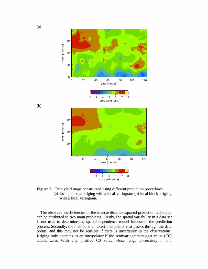
Local Kriging with local variograms (Figure 7a) restore some of the localvariability because the changes in spatial dependence between the localneighbourhoods is included. Changing the map model from point estimates toestimates representing the weighted average yield in a 20 metre block around eachprediction point (Figure 7b) removes some of this variability from the estimates.

That the form of spatial prediction chosen for map construction may besignificantly influential on the final prediction surface is not a new concept. Anumber of studies (e.g. Laslett et al. (1987), Wollenhaupt et al. (1994), Weber &Englund (1994), Whelan et al. (1996), Gotway et al. (1996)) show that in generalinverse distance techniques are sensitive to the degree of inherent variability in adata set, the neighbourhood population used in each prediction and the power ofdistance used in the weighting calculation. Alternatively, the accuracy of ordinarykriging generally displays little sensitivity to the variability in the data sets andthe accuracy of the estimates improves with increasing neighbourhoodpopulations.

(a)

0 20 40 60 80 100 120

60

40

20

0

east (metres)

nort

h (m

etre

s)

(b)

0 20 40 60 80 100 120

60

40

20

0

east (metres)

nort

h (m

etre

s)

(c)

0 20 40 60 80 100 120

60

40

20

0

east (metres)

nort

h (m

etre

s)

2 3 4 5 6 7 8crop yield (t/ha)

Figure 6. Crop yield maps constructed using different prediction procedures.(a) local mean (b) inverse distance-squared (c) local punctual krigingwith a global variogram.

(a)

0 20 40 60 80 100 120

60

40

20

0

east (metres)

nort

h (m

etre

s)

2 3 4 5 6 7 8crop yield (t/ha)

(b)

0 20 40 60 80 100 120

60

40

20

0

east (metres)

nort

h (m

etre

s)

3 4 5 6 7 8crop yield (t/ha)

Figure 7. Crop yield maps constructed using different prediction procedures.(a) local punctual kriging with a local variogram (b) local block kriging

with a local variogram.

The observed inefficiencies of the inverse distance squared prediction techniquecan be attributed to two main problems. Firstly, the spatial variability in a data setis not used to determine the spatial dependence model for use in the predictionprocess. Secondly, the method is an exact interpolator that passes through the datapoints, and this may not be sensible if there is uncertainty in the observations.Kriging only operates as an interpolator if the semivariogram nugget value (C0)equals zero. With any positive C0 value, close range uncertainty in the

observations will be reflected in the kriged surface. Such uncertainty may arise ineither the value of the observed attribute or its spatial location.

This point is often overlooked in assessing the suitability of predictiontechniques but should be a given a high priority in PA owing to the potential (andreal) errors associated with real-time sensors and GPS receivers (Lark et al.(1997); Whelan and McBratney (2002); Arslan and Colvin (2002)). In such cases,block kriging estimates for an area should prove extremely useful in reducing thecarryover of errors into the final maps. Block kriging also offers a robust methodof estimating values for an area that represents the smallest differentiallymanageable land unit in a farming operation (usually governed by implementwidth and operational dynamics).

Block kriging may be undertaken using a global semivariogram but once thenumber of data points rises above 500 it seems wasteful to assume a singlesemivariogram within the field. A global semivariogram may prove too restrictivein its representation of local spatial structure whereas local semivariogramestimation and kriging offers the ability to preserve the true local spatialvariability in the predictions. If the chosen neighbourhood is reasonably small, theuse of local semivariograms should also negate the possible requirement for trendanalysis and removal prior to semivariogram estimation and kriging.

A further advantage in the use of kriging techniques lies in the provision of aprediction variance estimate (Laslett et al., 1987; Brus et al., 1996) which may beused to produce confidence limits on the predicted values. The reporting of suchlimits should be mandatory for digital maps as they will have importantramifications on the extrapolation of management information (Whelan andMcBratney (1999); Cuppit and Whelan (2001). The uncertainty may also be usedto determine the most suitable mapping class delineations in digital maps. Forexample, if the 95% confidence interval in crop yield estimates is +/- 1.0 t/ha,classifying a field using classes less than 1.0 t/ha would be misleading. Aclassification system based on the uncertainty in the yield data may prove usefulin the future.

On the other hand, criticisms that have been levelled at the kriging techniques'complexity and related computational expense (e.g. Murphy et al., 1995).Astoundingly, this one line of criticism has apparently overridden all theadvantages discussed above, and led to the general acceptance of the inversedistance method as the prediction method of choice in the emerging mappingpackages for Precision Agriculture. While there may be some instances where aprediction map is required quickly (e.g. soil attribute maps for interpolation tofertiliser application maps), at present the author believes this is not a rationalreason for discarding the advantages incumbent with kriging techniques.Certainly for crop yield maps, the computational time would be far outweighed bythe single fact that the map represents a great deal of time, effort and expensetaken to grow a crop. Ultimately, it is the integration of an entire seasons cropgrowth information.

Where the computational expense may become important (and indeed thechoice of prediction technique possibly unimportant) is when the observationsampling scheme is inadequate in terms of sample size, sample strategy, or both.Sample size is probably considered the most crucial parameter (Englund et al.1992) with an increasing number of observations generally offering greaterprediction accuracy. Numerous studies on the effect of sample strategy forregionalised variables have been reported since the early theoretical work ofMcBratney et al. (1981). The general axiom to emerge is that sampling schemeswhich fail to produce a sample set representative of the actual spatial variability inthe attribute of interest will hinder accurate prediction by any method. Data setsfrom calibrated real-time sensors should not fall into this category, but traditionalsoil sampling operations may produce such data.

CONCLUDING REMARKS

Spatial prediction methods used in PA should accurately represent the spatialvariability of sampled field attributes and maintain the principle of minimuminformation loss. However, data used in any spatial prediction procedure shouldbe of known precision and that precision used to guide the choice of spatialpredictor. Due to imprecision in crop yield measurement and within-fieldlocation, interpolators (exact spatial predictors) are generally not optimal.

The results presented show that the form of spatial prediction chosen formapping yield has a significant influence on the final prediction surface. Localkriging using a local variogram appears well suited as a spatial prediction methodfor dense data-sets. In particular, local block kriging reduces the estimateuncertainty when compared with punctual kriging and may be an optimalmapping technique for the current generation real-time yield and soil sensors.

Ultimately, any software devised for spatial prediction in precision agricultureapplications should include options that will optimally support the managementdecisions that will be formulated upon the prediction results.

VESPER is available as shareware from the ACPA atwww.usyd.edu.au/su/agric/acpa

REFERENCES

Akaike, H. (1973). Information theory and an extension of maximum likelihoodprinciple. In B.N. Petrov & F. Csáki (ed.), Second International Symposiumon Information Theory. Akadémia Kiadó, Budapest. pp 267-281.

Arslan, S., Colvin, T.S. (2002). Grain yield mapping: yield sensing, yieldreconstruction and errors. Precision Agriculture 3 : 135-154.

Brus, D.J., de Gruijter, J.J., Marsman, B.A., Visschers, R., Bregt , A.K.,Breeuwsma, A., Bouma, J. (1996). The performance of spatial interpolationmethods and choropleth maps to estimate soil properties at points: a soilsurvey case study. Environmetrics 7: 1-16.

Burgess, T.M., Webster, R. (1980). Optimal interpolation and isarithmic mappingof soil properties. II. Block kriging. J. Soil Sci. 31 : 333-341.

Cupitt, J., Whelan, B.M. (2001). Determining potential within-field cropmanagement zones. In G. Grenier and S. Blackmore (ed.), ECPA 2001,Proceedings of the 3rd European Conference on Precision Agriculture,Montpellier, France, agro-Montpellier, Montpellier, France pp 7-12.

Englund, E.J., Weber, D.D. and Leviant, N. (1992). The effects of samplingdesign parameters on block selection. Math. Geol. 24: 329-343.

Goodchild, M.F. (1992). Geographical data modelling. Computers andGeosciences 18: 401-408.

Gotway, C.A., Ferguson, R.B. & Hergert, G.W. & Peterson, T.A. (1996).Comparison of kriging and inverse-distance methods for mapping soilparameters. Soil Sci. Soc. Am. J. 60: 1237-1247.

Haas, T.C. (1990). Kriging and automated semivariogram modelling within amoving window. Atmospheric Environment 24A: 1759-1769.

Laslett, G.M., McBratney, A.B., Pahl, P.J., Hutchinson, M.F. (1987). Comparisonof several spatial prediction methods for soil pH. J. Soil Sci. 38: 325–341.

Lark, R.M., Stafford, J.V., Bolam, H.C. (1997). Limitations on the spatialresolution of yield mapping for combinable crops. J. Agric. Engng Res. 66:183-193.

McBratney, A.B., Webster, R., Burgess, T.M. (1981). The design of optimalsampling schemes for local estimation and mapping of regional variables – I :theory and method. Computers and Geosciences 7: 331-334.

Murphy, D.P., Schnug, E., Haneklaus, S. (1995). Yield mapping – a guide toimproved techniques and strategies. In P.C. Robert, R.H. Rust & W.E. Larson(ed.), Site-Specific Management for Agricultural Systems: Proceedings of the2nd International Conference on Precision Agriculture, ASA/CSSA/SSS,Madison. pp. 32-47.

Weber, D.D., Englund, E.J. (1994). Evaluation and comparison of spatialinterpolators II. Math. Geol. 26: 589-603.

Whelan, B.M., McBratney, A.B. (1997). Sorghum grain-flow convolution withina conventional combine harvester. In J.V. Stafford (ed.), Precision Agriculture1997, Bios, Oxford, England. pp 759-766.

Whelan, B.M., McBratney, A.B. (1999). Prediction uncertainty and implicationsfor digital map resolution. In P.C. Robert, R.H. Rust & W.E. Larson (ed.),Precision Agriculture, Proceedings of the 4th International Conference onPrecision Agriculture, ASA/CSSA/SSSA, Madison, Wisconsin. pp 1185-1196.

Whelan, B.M., McBratney, A.B. (2002). A parametric transfer function for grain-flow within a conventional combine harvester. Precision Agriculture 3 : 123-134.

Whelan, B.M., McBratney, A.B., Viscarra Rossel, R.A. (1996). Spatial predictionfor Precision Agriculture. In P.C. Robert, R.H. Rust & W.E. Larson (ed.),Precision Agriculture: Proceedings of the 3rd International Conference onPrecision Agriculture, ASA/CSSA/SSS, Madison. pp. 331-342.

Wollenhaupt, N.C., Wolkowski, R.P., Clayton, M.K. (1994). Mapping soil testphosphorus and potassium for variable-rate fertilizer application. J. Prod.Agric. 7 : 441-448.