Vertical structure, energetics, and dynamics of the Brazil Current System at 22°S-28°S

Vertical structure, energetics, and dynamics of the Brazil CurrentSystem at 22�S–28�S

Cesar B. Rocha,1,2 Ilson C. A. da Silveira,1 Belmiro M. Castro,1 and Jose Antonio M. Lima3

Received 24 May 2013; revised 28 November 2013; accepted 2 December 2013; published 7 January 2014.

[1] We use four current meter moorings and quasi-synoptic hydrographic observations inconjunction with a one-dimensional quasi-geostrophic linear stability model to investigatedownstream changes in the Brazil Current (BC) System between 22�S and 28�S. The dataset depict the downstream thickening of the BC. Its vertical extension increases from 350 mat 22.7�S to 850 m at 27.9�S. Most of this deepening occurs between 25.5�S and 27.9�S andis linked to the bifurcation of the South Equatorial Current at intermediate depths (Santosbifurcation), which adds the Antarctic Intermediate Water flow to the BC. Geostrophicestimates suggest that the BC transport is increased by at least 4.3 Sv (�70%) to the southof that bifurcation. Moreover, the Santos bifurcation is associated with a substantialincrease in the barotropic component of the BC System. On average, the water columnaverage kinetic energy (IKE) is 70% baroclinic to the north and 54% barotropic to the southof the bifurcation. Additionally, the BC shows conspicuous mesoscale activity off southeastBrazil. The water column average eddy kinetic energy accounts for 30–60% of the IKE.Instabilities of the mean flow may give rise to these mesoscale fluctuations. Indeed, thelinear stability analysis suggests that the BC System is baroclinically unstable between 22�Sand 28�S. In particular, the model predicts southwestward-propagating fastest growingwaves (�190 km) from 25.5�S to 27.9�S and quasi-standing most unstable modes (�230km) at 22.7�S. These modes have vertical structures roughly consistent with the observededdy field.

Citation: Rocha, C. B., I. C. A. da Silveira, B. M. Castro, and J. A. M. Lima (2014), Vertical structure, energetics, and dynamics ofthe Brazil Current System at 22�S–28�S, J. Geophys. Res. Oceans, 119, 52–69, doi:10.1002/2013JC009143.

1. Introduction

[2] The Brazil Current (BC) is the subtropical westernboundary current (WBC) of the South Atlantic. Most of ourcurrent understanding of the BC relies on quasi-synoptichydrographic observations [e.g., Campos et al., 1995; daSilveira et al., 2004]. Studies based on analysis of currentmeter time series are rare [M€uller et al., 1998; da Silveiraet al., 2008], and this has constrained the development of aquantitative description of the BC.

[3] As it flows over the southeast Brazil slope (�20�S–25�S), the BC presents a vertical structure very differentfrom that of other WBCs at similar latitudes [da Silveiraet al., 2008]. In this region, the BC is depicted as a shallowcurrent (�400 m), transporting tropical water (TW) at sur-

face/near-surface levels and South Atlantic Central Water(SACW) at pycnocline levels [Campos et al., 1995; da Sil-veira et al., 2000]. Underneath the BC (�(500–1200) m),there is an opposing flow, the intermediate western bound-ary current (IWBC), transporting mainly Antarctic Interme-diate Water (AAIW) to the north/northeast [e.g., Evans andSignorini, 1985; da Silveira et al., 2004]. This unique sub-tropical WBC System is linked to the depth-dependentbifurcation system of the South Equatorial Current over theBrazilian continental margin [e.g., Stramma and England,1999]. At intermediate levels, float observations suggestthat the so-called Santos bifurcation occurs between 25�Sand 27�S [Böebel et al., 1999; Legeais et al., 2013]. To thesouth of that bifurcation (�28�S), the entire water columnover the slope flows to the south/southwest [M€uller et al.,1998], and the BC transports TW, SACW, and AAIW.

[4] Few studies have addressed the BC dynamics. da Sil-veira et al. [2008] showed that the mean BC System at22.7�S is essentially a first baroclinic mode flow. Further-more, these authors argued that the vertical shear associatedwith the BC/IWBC opposing flows likely makes the BCSystem prone to baroclinic instability, and that a one-dimensional quasi-geostrophic (QG) model successfullypredicted the length scales of the mesoscale variability inthis region. Additionally, the QG linear model predictedunstable modes with very small propagation speeds,

1Instituto Oceanogr�afico, Universidade de S~ao Paulo, S~ao Paulo, Brazil.2Now at Scripps Institution of Oceanography, University of California,

San Diego, La Jolla, California, USA.3Centro de Pesquisas e Desenvolvimento Leopoldo A. Miguez de

Mello, Petr�oleo Brasileiro S. A., Rio de Janeiro, Brazil.

Corresponding author: C. B. Rocha, Scripps Institution of Oceanogra-phy, University of California, San Diego, 9500 Gilman Drive, La Jolla,CA 92093-0208, USA. ([email protected])

©2013. American Geophysical Union. All Rights Reserved.2169-9275/14/10.1002/2013JC009143

52

JOURNAL OF GEOPHYSICAL RESEARCH: OCEANS, VOL. 119, 52–69, doi:10.1002/2013JC009143, 2014

info:doi/10.1002/2013JC009143

http://dx.doi.org/10.1002/2013JC009143

roughly in agreement with the few observed events in seasurface temperature imagery [Garfield, 1990]. Mano et al.[2009] described the energy flux during the growth of acyclonic meander in a primitive-equation (PE) numericalsimulation of the BC System in the same region. While thebasic phenomenology described by these authors is qualita-tively consistent with da Silveira et al.’s [2008] QG baro-clinic instability arguments, the BC meandering seems tobe much more complicated in the PE model. Additionally,Oliveira et al. [2009] studied the surface energetics of theBC from surface drifter buoys. These authors showed thatthe (surface) eddy kinetic energy is significant along theBC path. Based on barotropic conversion estimates, Oli-veira et al. [2009] argued that part of the BC variabilitymay be accounted for by barotropic instabilities.

[5] It is relatively well accepted that the BC undergoeschanges on its downstream path off southeast Brazil [M€ulleret al., 1998; da Silveira et al., 2000]. Nonetheless, no system-atic quantifications of these changes are available to date. Inaddition, the BC is generally associated with rich mesoscaleactivity within this region [e.g., Campos et al., 1995, 2000;da Silveira et al., 2008], but quantitative estimates of itsimportance are limited to the surface [Oliveira et al., 2009].

[6] Here, we investigate downstream changes in the BCbetween 22�S and 28�S. The specific questions are: (1a)How much does the BC thicken and (1b) how much does theBC transport increase within this region? (2a) What is thepartition between barotropic and baroclinic components inthe BC System and (2b) what are the downstream changeson this partition? (3) How much of the BC System energy isin the eddy field? (4a) What are the downstream changes inthe BC System linear stability properties and (4b) can thepredictions of the stability analysis account for the changingcharacter of the perturbations in the downstream direction?

[7] To address these questions, we analyze four currentmeter mooring records, not necessarily spanning the sametime period, but nonetheless covering the study region withunprecedented along-coast resolution. The analysis of thesemoorings within the same framework combined with quasi-synoptic hydrographic observations yields a comprehensive(but limited) description of the BC off southeast Brazil. Inaddition, application of a QG model to the observationsprovides insight into the dynamics governing the BC vari-ability at mesoscales.

2. Mooring Observations

2.1. The Data Set

[8] The four current meter moorings were located inthe BC domain (Figure 5 and Table 1) spanning the south-

east Brazil (22�S–28�S): MARLIM (22.7�S, 1250 m),DEPROAS FBS (24.15�, 1200 m; hereafter DFBS),COROAS 3 (25.5�, 1000 m; hereafter C3), and WOCEACM12 333 (27.9�S, 1200 m; hereafter W333). Theserecords span 1–2 years; thus the BC mesoscale variabilityis expected to be well resolved.

[9] The velocity record at each current meter was low-pass filtered using a Lanczos-cosine filter [e.g., Emery andThomson, 2001]. The cutoff period was set at 40 h, whichis 30% greater than the inertial period at the northernmostmooring (�31 h), and therefore near-inertial and superiner-tial motions were filtered out. Individual current meter gapswere filled using the empirical orthogonal functions (EOF)of the velocity anomaly time series. This technique waschosen because it does not change the data statistics [Beck-ers and Rixen, 2003; Dengler et al., 2004; Schott et al.,2005].

[10] The C3 mooring had a gap in all four instruments (4May 1993 to 18 June 1993), which was filled in two steps.The uppermost instrument velocity series was filled usingthe EOF method (horizontally) with the uppermost instru-ment of an adjacent mooring which had a spectrum coher-ent with the C3 mooring uppermost record. The remaininggaps in the other three instruments were then filled usingthe EOFs (vertically). Such a twofold filling process wasnot possible for the 30 day gap (27 May 1992 to 23 June1992) at the MARLIM mooring since concurrent adjacentmoorings were not available.

[11] The BC flow is clearly depicted in the upper 300 mat the MARLIM mooring (Figure 1), although strong cur-rent reversals are also observed in the upper levels. Asnear-inertial and superinertial motions were filtered out, itis likely that these reversals are due to strong BC meander-ing events [da Silveira et al., 2008]. The IWBC is consis-tently depicted from 650 to 1050 m flowing to thenortheast. No current reversals are observed in the IWBCdomain, suggesting that the meandering is mainly confinedto the upper levels.

[12] The time series for the DFBS mooring depicts amuch more convoluted scenario (Figure 2). The threeuppermost instruments present strong current reversalsthroughout the record. At intermediate levels (800 and1000 m instruments) this mooring depicts the IWBC flow-ing to the northeast. However, it should be noted that theIWBC seems more variable at this location than at theMARLIM mooring. The flow at 500 m presents reversalsthroughout the record, suggesting that the separation of theBC-IWBC occurs near this depth.

[13] At the C3 mooring (Figure 3), the BC is depicted inthe three upper instruments as a persistent southwest flow.

Table 1. Main Characteristics for the MARLIM, DFBS, C3, and W333 Mooringsa

Isobath (m) Instruments (m) Record (Days) Reference

MARLIM (22.7�S, 40.2�W) 1250 50; 100; 250; 350; 450; 650;750; 950; 1050

308 (Feb 1992 to Dec 1992) da Silveira et al. [2008]

DFBS (24.15�S, 42.4�W) 1200 30; 50; 70; 500;800; 1000 482 (Jan 2003 to May 2004) —C3 (25.5�S, 44.9�W) 1000 29; 91; 293; 698 455 (Dec 1992 to Mar 1994) Campos et al. [1996]W333 (27.9�S, 46.7�W) 1200 60; 77; 95; 112; 138; 155; 173;

230; 475; 680; 885693 (Jan 1991 to Nov 1992) M€uller et al. [1998]

aNote that da Silveira et al. [2008] only used the second half of the MARLIM record and Campos et al. [1996] only quoted the C3 mooring results.

ROCHA ET AL.: ON THE BRAZIL CURRENT AT 22�S–28�S

53

Although the BC is also highly variable at this location,just one strong current reversal was observed (March1993). The C3 mooring has just one instrument at interme-diate depths (693 m), which depicts a northeastward flow.This suggests that the IWBC is already well formed at thislocation, as suggested by Campos et al. [1996]. However, itis important to note that, contrary to what is observed at theMARLIM mooring, the northeast flow at the C3 mooring isclearly highly variable.

[14] Farther downstream at the W333 mooring (Figure4), the BC is depicted flowing southward/southwestwardfrom the surface down to the instrument at 670 m depth. Atthis location, just two prominent velocity vector reversalsare depicted in the BC (January 1991 and October 1992).In addition, the flow at the deepest instrument (885 m) ishighly variable and presents no preferential direction.Thus, there is no evidence of the IWBC, suggesting thatthis mooring is located to the south of the Santos bifurca-

tion. This is consistent with a recent description on thebasis of float observations [Legeais et al., 2013].

2.2. Basic Velocity Statistics

[15] A well-known caveat in mooring data analysis isthat instruments, particularly those near the surface, mayexperience substantial drawn down during highly energeticevents. This can bias statistical analyses, but there seems tobe no easy solution for such problem [Wunsch, 1997]. Forthe present data set, we have reliable pressure records onlyfor the W333 mooring. At this location, the vertical dis-placements are typically fairly small (<30 m about thenominal depth), but can be as large as 175 m in oneextreme short-lived case. The 230 m instrument was 90%of the time at depths shallower than 255 m, which repre-sents a displacement of 10% about its nominal depth.Assuming that the other three moorings experienced similarsmall vertical displacements, the statistics presented beloware deemed reliable.

[16] It is convenient to rotate the velocity vector into alocal along-front/cross-front coordinate system since this

Apr92 Jul92 Oct92 Jan93

1 m s−1

50m

100m

250m

350m

450m

650m

750m

950m

1050m

Figure 1. MARLIM mooring velocity time series. Only one vector per day is plotted. For reference,the north points upward.

Jan03 Apr03 Jul03 Oct03 Jan04 Apr04

1 m s−1

30m

50m

70m

500m

800m

1000m

Figure 2. Similar to Figure 1, but for the DFBS mooring.

Jan93 Apr93 Jul93 Oct93 Jan94 Apr94

1 m s−1

21m

91m

293m

698m

Figure 3. Similar to Figure 1, but for the C3 mooring.


54

facilitates the intercomparison among the moorings. TheBC thermal front marks the BC inshore border [Garfield,1990; da Silveira et al., 2008]. The along-front directionwas computed based on the angle between geographicnorth and the BC mean thermal front, which was computedusing the estimates of Garfield [1990] and da Silveira et al.[2008] (Figure 5); at the DFBS mooring, where those esti-mates diverge, we used the mean thermal front from the lat-ter authors. Hereafter, u and v will be used to refer to thelocal cross-front and along-front (low-pass filtered) veloc-ity components, respectively.

[17] For each mooring, basic statistics (mean and stand-ard deviation) for the velocity components were estimated.In order to assess the robustness of these estimates, stand-ard errors were calculated [e.g., Glover et al., 2011]. Thestandard error depends on the standard deviation as well ason the effective number of degrees of freedom (eDOF).The eDOF was computed by dividing the record length bythe (autocorrelation) integral time scale [Glover et al.,

2011]. Integral time scale and eDOF were computed indi-vidually for each velocity component at each current meter.

[18] The time scales proved to be anisotropic, which ledto significant differences in the eDOF in each direction.The along-front integral time scale varies from 6 to 9 days,whereas the cross-front integral time scale ranges from 4 to5 days. Moreover, eDOF varies substantially (�30–170)from mooring to mooring due to differences in the durationof the records.

[19] Mean and standard deviation along with their uncer-tainties are presented in Tables (2–5), and the mean veloc-ity vectors for the instruments closest to 50 and 700 m aredisplayed in Figure 5. The mean flow essentially followsthe mean BC thermal front, which is parallel to the localisobath at all moorings except at the DFBS mooring (Fig-ure 5). Near this mooring, the mean BC front veers west-ward along the 200 m isobath; the veering of the deeperisobaths is gentler, so that the IWBC flow at this locationfollows the local isobath, which is not in the same directionas the BC front.

[20] The near-surface BC along-front mean velocity ishighest at the C3 mooring (20.51 6 0.05 m s21 at 29 m),as compared to the W333 mooring (20.34 6 0.04 m s21 at60 m) and MARLIM mooring (20.31 6 0.12 m s21 at 50m). This suggests that the C3 mooring is closer to the BCcore than the other moorings. Furthermore, at the DFBSmooring, the mean along-front BC velocity is much weaker(20.17 6 0.14 m s21 at 50 m). Near-surface along-frontstandard deviation is higher at the DFBS mooring(0.39 6 0.10 m s21 at 50 m) and at the MARLIM mooring(0.37 6 0.03 m s21 at 50 m), exceeding the mean values attheir respective depths, thus confirming the high variability

Jan91 Apr91 Jul91 Oct91 Jan92 Apr92 Jul92 Oct92

1 m s−1

60m

95m

155m

230m

475m

680m

885m

Figure 4. Similar to Figure 1, but for the W333 mooring.The velocity records at 77, 112, 138, and 173 m areomitted.

Figure 5. Mean velocity vector for instruments closest to50 m (red) and 700 m (blue) at each mooring. The meanthermal front estimated by Garfield [1990] (diamonds) andda Silveira et al. [2008] (circles) are also shown. Gray tri-angles represent hydrographic stations.

Table 2. Velocity Statistics for the MARLIM Mooringa

InstrumentAlong Front Cross Front

(m) Mean (m s21) Std (m s21) Mean (m s21) Std (m s21)

50 20.31 6 0.12 0.37 6 0.08 0.07 6 0.08� 0.25 6 0.06100 20.26 6 0.11 0.36 60.08 0.08 6 0.07 0.23 6 0.05250 20.08 6 0.06 0.20 6 0.04 0.08 6 0.04 0.13 6 0.03350 0.02 6 0.05� 0.16 6 0.03 0.05 6 0.03 0.09 6 0.02450 0.08 6 0.03 0.10 6 0.02 0.07 6 0.03 0.09 6 0.02650 0.19 6 0.02 0.07 6 0.02 0.00 6 0.01� 0.05 6 0.01750 0.19 6 0.02 0.07 6 0.01 0.03 6 0.02 0.06 6 0.01950 0.22 6 0.03 0.08 6 0.02 0.03 6 0.01 0.04 6 0.011050 0.21 6 0.03 0.10 6 0.02 0.02 6 0.01 0.03 6 0.01

aThe 95% confidence interval was computed by doubling the standarderror. Stars indicate those estimates that are not statistically significant.

Table 3. Similar to Table 2, but for the DFBS Mooring



30 20.17 6 0.14 0.38 6 0.10 0.02 6 0.04� 0.17 6 0.0350 20.17 6 0.14 0.39 6 0.10 0.02 6 0.04� 0.18 6 0.0370 20.16 6 0.14 0.40 6 0.10 0.02 6 0.04� 0.19 6 0.03500 0.04 6 0.04� 0.12 6 0.03 0.04 6 0.01 0.06 6 0.01800 0.11 6 0.03 0.08 6 0.02 0.07 6 0.01 0.04 6 0.011000 0.09 6 0.03 0.09 6 0.02 0.05 6 0.01 0.04 6 0.01


55

at these locations. Relatively high near-surface along-frontstandard deviation values are also observed at the C3 moor-ing (0.24 6 0.04 m s21 at 29 m) and at the W333 mooring(0.23 6 0.03 m s21 at 60 m). The high uncertainties associ-ated with the mean estimates at near-surface instruments atthe DFBS and MARLIM moorings are a consequence ofthe small eDOF and the high standard deviation at thoselocations. In particular, the mean values for the three upperinstruments at the DFBS mooring have low statistical sig-nificance. There are too few eDOF to estimate a reliablealong-front mean. Physically, the BC experiences high var-iability in this region, as if continuously adjusting to con-serve its potential vorticity after overshooting thecontinental margin past Cape Frio (�23�S) [Campos et al.,1995]. Therefore, it is very difficult to establish a ‘‘station-ary’’ flow at this location.

[21] The BC cross-front mean velocity component isvery weak at all moorings (Tables 2–5). Although slightlysmaller than those estimates for the along-front component,the standard deviation for the cross-front component is sig-nificant, suggesting that the time-varying flow is less aniso-tropic than the time-mean flow.

[22] At intermediate depths, the MARLIM and DFBSmoorings consistently depict a mean IWBC flowing north-eastward. Maximum IWBC along-front velocity isobserved in the north of the domain, at the MARLIM moor-ing (0.22 6 0.03 m s21 at 950 m). At the DFBS mooring,maximum along-front IWBC velocity is observed at 800 m(0.11 6 0.02 m s21). At the C3 mooring, the single instru-ment at intermediate depths depicts a relatively weak (butsignificant) northward/eastward flow (0.09 6 0.03 m s21 at698 m). The along-front IWBC velocity component seemsto present relatively small (relative to the mean) standarddeviation values at the MARLIM mooring (0.08 6 0.02 ms21 at 950 m), but slightly greater at the DFBS mooring

(0.08 6 0.02 m s21 at 800 m). At the C3 mooring, thealong-front IWBC standard deviation (0.13 6 0.02 m s21 at698 m) exceeds the mean value.

[23] In contrast, a mean southwestward along-front flowis observed at intermediate depths at the W333 mooring(20.06 6 0.02 m s21 at 680 m), in agreement with M€ulleret al.’s [1998] estimates. No mean northward/eastwardflow is observed at this location. Relatively high along-front standard deviation values are observed at intermediatedepths at this mooring, exceeding the mean values(0.10 6 0.01 m s21 at 680 m).

[24] In summary, the basic statistics shows that the BCpresents significant variability off southeast Brazil, thuscorroborating the importance of mesoscale activity withinthis region. The mean along-front velocity measurementsalso depict the thickening of the BC, namely its down-stream growth in vertical extension. In order to betterdescribe this thickening process, we now turn to the projec-tion of the mean along-front velocity profile onto thedynamical modes.

2.3. The Thickening of the Brazil Current

[25] The mean along-front velocity at the discrete instru-ment depths were fit to the five gravest dynamical modesusing a Gauss-Markov estimate [e.g., Szuts et al., 2012].These modes were computed numerically using the meanstratification (N2 (z)) at each location. N2 (z) profiles wereestimated using the World Ocean Atlas 2009 climatology[Locarnini et al., 2010; Antonov et al., 2010]. As thedynamical modes and their derivatives are smooth [da Sil-veira et al., 2008], we argue that this is a consistent methodfor obtaining interpolated velocity profiles on an equi-spaced grid. These profiles are further used along with theN2 (z) profile as inputs for the linear stability model (sec-tion 5.1).

[26] The interpolated along-front velocity profiles clearlyshow the thickening of the BC (Figure 6). Accordingly, theBC is 350 m deep at the MARLIM mooring, 550 m deep atthe C3 mooring, and 850 m deep at the W333 mooring.Although the mean along-front velocity presents low statis-tical significance at the DFBS mooring, the BC verticalextension (�400 m) seems to be consistent at this location.

[27] Another interesting feature that is clear in the syn-thesized velocity profiles concerns the downstream changesin mean flow vertical shear. Accordingly, the BC Systempresents a much more prominent shear at the MARLIM,DFBS, and C3 moorings than at the W333 mooring, thussuggesting that the Santos bifurcation is associated with astrong increase in the BC System barotropic component.

3. Quasi-Synoptic Patterns

[28] In order to present a two-dimensional characteriza-tion of the downstream changes in the BC, we analyze theavailable hydrographic sections contemporary with themooring records (Table 6). The W333 does not presentvelocity measurements exactly concurrent to the A10cruise. While this cruise recovered the W333 mooring, thelast month (December 1992) of the mooring measurementswere disregarded during the quality control process. At thislocation, the mooring velocity compared to the geostrophicvelocity estimates represents those measurements made 1

Table 4. Similar to Table 2, but the for C3 Mooring



29 20.51 6 0.05 0.24 6 0.04 20.01 6 0.03� 0.12 6 0.0291 20.49 6 0.06 0.24 6 0.04 20.05 6 0.03 0.12 6 0.02293 20.23 6 0.04 0.17 6 0.03 20.03 6 0.01 0.06 6 0.01698 0.09 6 0.03 0.13 6 0.02 0.00 6 0.01� 0.03 6 0.01

Table 5. Similar to Table 2, but for the W333 Mooring.



60 20.34 6 0.04 0.23 6 0.03 20.07 6 0.03 0.17 6 0.0277 20.34 6 0.05 0.23 6 0.03 20.06 6 0.04 0.17 6 0.0395 20.34 6 0.05 0.23 6 0.03 20.07 6 0.04 0.17 6 0.03112 20.346 0.05 0.23 6 0.03 20.07 6 0.03 0.17 6 0.02138 20.336 0.05 0.23 6 0.03 20.06 6 0.03 0.16 6 0.02155 20.326 0.05 0.22 6 0.03 20.06 6 0.03 0.15 6 0.02173 20.316 0.05 0.21 6 0.03 20.06 6 0.03 0.14 6 0.02230 20.29 6 0.05 0.20 6 0.03 20.06 6 0.03 0.13 6 0.02475 20.15 6 0.03 0.12 6 0.02 20.04 6 0.01 0.07 6 0.01680 20.06 6 0.02 0.10 6 0.01 20.02 6 0.01 0.06 6 0.01885 0.00 6 0.02� 0.11 6 0.01 20.02 6 0.01 0.05 6 0.01


56

month earlier (30 November 1992), and hence this compar-ison should be interpreted with caution.

[29] Geostrophic velocities are computed relative to anisopycnal level of no motion [e.g., Stramma et al., 1995].There is no such reason to expect that the velocity is zeroalong these isopycnals, although it is likely. This is a sourceof inaccuracy in the geostrophic velocity estimates, andcare should be taken in interpreting the results. Nonethe-less, this method proved to produce a consistent (lowerbound) transport estimates without requiring arbitraryshoreward extrapolations of the geopotential anomalies tocompute velocities on the inner slope. The isopycnal usedfor reference is the one that crosses the mooring at the cor-responding no-motion depth at the mooring location. Themooring data was averaged over the same time period asthe section occupation, typically 3 days.

[30] At the MARLIM, DFBS, and C3 moorings, the levelof no motion is associated with the depth that separates theBC from the IWBC flow. The reversal depth is estimatedfrom the mooring velocity profile synthesized using thedynamical modes in a fashion similar to the mean flow

(section 2.3). At these locations, similar results are obtainedby setting an arbitrary level of no motion (not shown). Atthe W333 mooring the IWCB is not present, and hencethere is no such reversal depth. We therefore consider thelevel of no motion as that of the deepest instrument (885m), which presented fairly weak velocities during thehydrographic cruise occupation (�0.03 m s21). At thismooring, similar results (pattern and transport) are obtainedby computing the geostrophic velocities referenced to thebottom (not presented).

[31] The BC geostrophic transport is estimated consider-ing this current as the southward flow delimited by the20.05 m s21 isotach, which was the weakest contour thatdefined the BC in all sections. Hence, the transport valuespresented here represent conservative estimates. The geo-strophic velocity estimates are compared to the mooringvelocities averaged over the cruise period. For the DFBS,C3, and W333 moorings, which are located between twogeostrophic velocity profiles, the mooring velocity is com-pared against the mean estimate between the two adjacentprofiles.

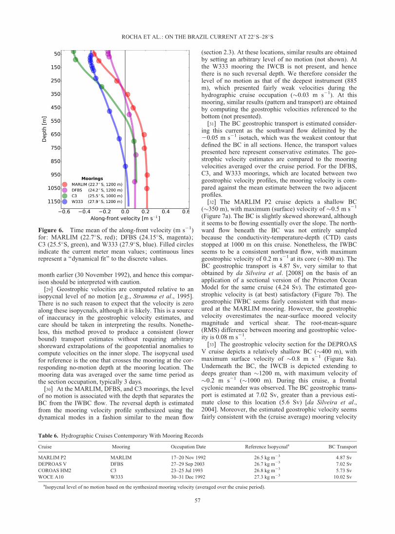
[32] The MARLIM P2 cruise depicts a shallow BC(�350 m), with maximum (surface) velocity of �0.5 m s21

(Figure 7a). The BC is slightly skewed shoreward, althoughit seems to be flowing essentially over the slope. The north-ward flow beneath the BC was not entirely sampledbecause the conductivity-temperature-depth (CTD) castsstopped at 1000 m on this cruise. Nonetheless, the IWBCseems to be a consistent northward flow, with maximumgeostrophic velocity of 0.2 m s21 at its core (�800 m). TheBC geostrophic transport is 4.87 Sv, very similar to thatobtained by da Silveira et al. [2008] on the basis of anapplication of a sectional version of the Princeton OceanModel for the same cruise (4.24 Sv). The estimated geo-strophic velocity is (at best) satisfactory (Figure 7b). Thegeostrophic IWBC seems fairly consistent with that meas-ured at the MARLIM mooring. However, the geostrophicvelocity overestimates the near-surface moored velocitymagnitude and vertical shear. The root-mean-square(RMS) difference between mooring and geostrophic veloc-ity is 0.08 m s21.

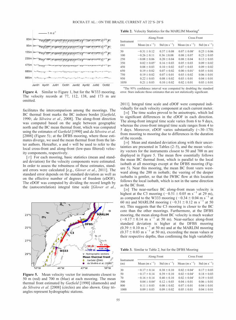
[33] The geostrophic velocity section for the DEPROASV cruise depicts a relatively shallow BC (�400 m), withmaximum surface velocity of �0.8 m s21 (Figure 8a).Underneath the BC, the IWCB is depicted extending todeeps greater than �1200 m, with maximum velocity of�0.2 m s21 (�1000 m). During this cruise, a frontalcyclonic meander was observed. The BC geostrophic trans-port is estimated at 7.02 Sv, greater than a previous esti-mate close to this location (5.6 Sv) [da Silveira et al.,2004]. Moreover, the estimated geostrophic velocity seemsfairly consistent with the (cruise average) mooring velocity

Figure 6. Time mean of the along-front velocity (m s21)for: MARLIM (22.7�S, red); DFBS (24.15�S, magenta);C3 (25.5�S, green), and W333 (27.9�S, blue). Filled circlesindicate the current meter mean values; continuous linesrepresent a ‘‘dynamical fit’’ to the discrete values.

Table 6. Hydrographic Cruises Contemporary With Mooring Records

Cruise Mooring Occupation Date Reference Isopycnala BC Transport

MARLIM P2 MARLIM 17–20 Nov 1992 26.5 kg m23 4.87 SvDEPROAS V DFBS 27–29 Sep 2003 26.7 kg m23 7.02 SvCOROAS HM2 C3 23–25 Jul 1993 26.8 kg m23 5.73 SvWOCE A10 W333 30–31 Dec 1992 27.3 kg m23 10.02 Sv

aIsopycnal level of no motion based on the synthesized mooring velocity (averaged over the cruise period).


57

(Figure 8b). The RMS difference between the synthesizedmooring velocity and the geostrophic velocity is 0.03 ms21. The major differences consist of an overestimation ofthe surface velocities and an underestimation of the veloc-ities close to the IWBC core (�1000 m).

[34] The HM2 cruise depicts a �450 m deep BC flowingsouthward, with maximum (surface) geostrophic velocityof �0.8 m s21 (Figure 9a). The IWBC is depicted as anorthward flow with maximum velocity of �0.15 m s21 atits core (�1000 m), thus weaker than that during the

Distance [km] relative to 100 m isobath

Dep

th [m

]

−0.8

−0.6

−0.4

−0.2

−0.1−0.05

0.05

0.050.05

0.05

0.1

0.1

0.1

0.1

0.15

0.15

0.15

0.2

DEPROAS V Sec. 5

27−29 Sep. 2003

Reference: 26.7 kg m−3

0 50 100 150

1200

1000

800

600

400

200

50

−0.5 0 0.51200

1100

1000

900

800

700

600

500

400

300

200

100

Cross−section velocity [m/s]

Dep

th [m

]

(b)

(a)

RM S = 0.03 m s − 1

Mooring

Geo. Velocity

Figure 8. Similar to Figure 7, but for the DEPROAS V cruise/DFBS mooring. As the mooring positionis not coincident with a geostrophic velocity profile (white triangles), the latter is taken as the averagebetween the profiles adjacent to the mooring position.

−0.5−0.4−0.3−0.2

−0.2−0.1−0.1

−0.0

5

−0.05

0.05

0.05

0.1

0.150.2


Dep

th [m

]

MARLIM P2

17−20 Nov. 1992

Reference: 26.5 kg m−3 (a)

40 60 80 100 120 140 160 180

1200

1000

800

600

400

200

50

−0.4 −0.2 0 0.2 0.4

1100

1000

900

800

700

600

500

400

300

200

100

Cross−section velocity [m/s]D

epth

[m]

(b)RM S = 0.08 m s − 1

Mooring

Geo. Velocity

Figure 7. (a) Geostrophic velocity for the MARLIM P2 cruise relative to an isopycnal level of nomotion (black line) and (b) comparison of geostrophic velocity and mooring velocity (time mean overthe period of the cruise). Black triangles represent the hydrographic stations. White triangles indicate thepositions used in the geostrophic velocity calculation. The green triangle represents the point (along thesection) closest to the MARLIM mooring. Gray dots indicate the current meter positions along the watercolumn.


58

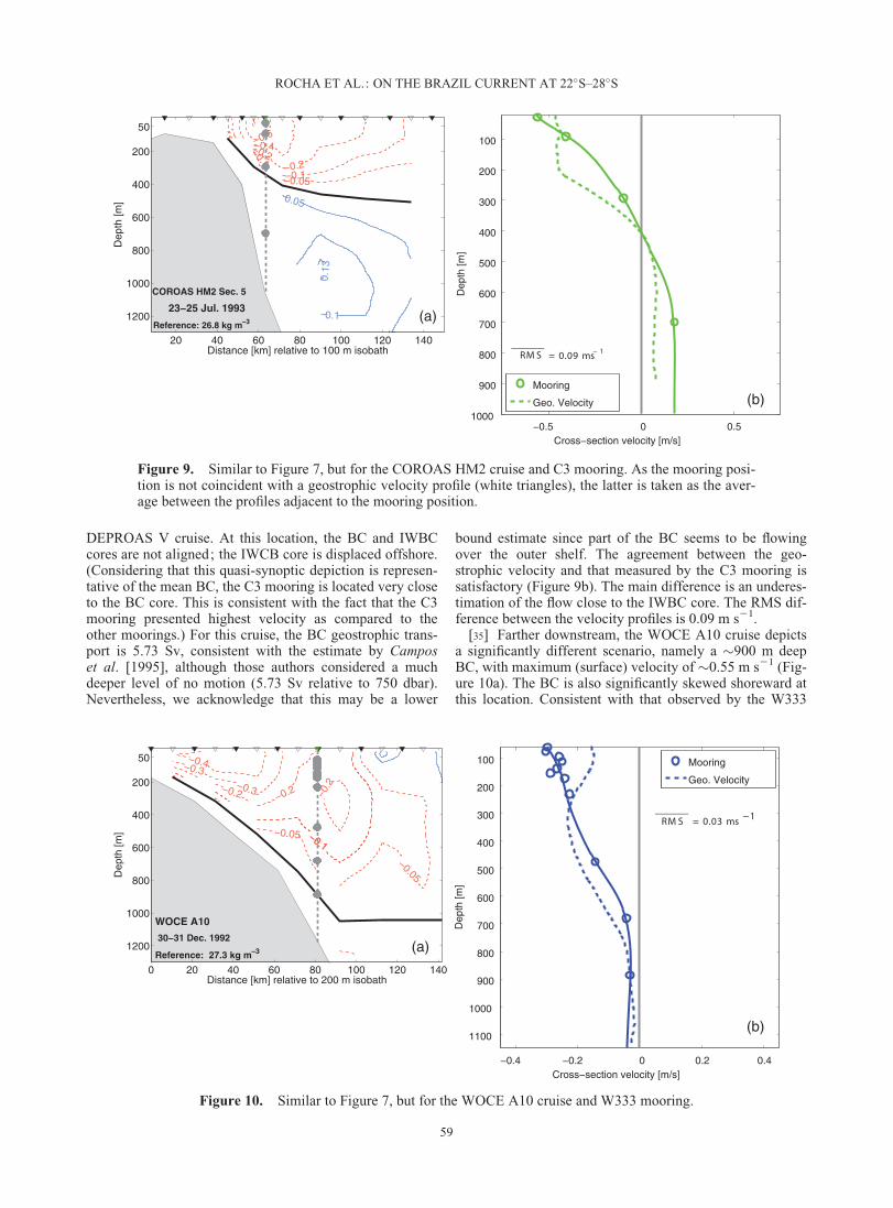
DEPROAS V cruise. At this location, the BC and IWBCcores are not aligned; the IWCB core is displaced offshore.(Considering that this quasi-synoptic depiction is represen-tative of the mean BC, the C3 mooring is located very closeto the BC core. This is consistent with the fact that the C3mooring presented highest velocity as compared to theother moorings.) For this cruise, the BC geostrophic trans-port is 5.73 Sv, consistent with the estimate by Camposet al. [1995], although those authors considered a muchdeeper level of no motion (5.73 Sv relative to 750 dbar).Nevertheless, we acknowledge that this may be a lower

bound estimate since part of the BC seems to be flowingover the outer shelf. The agreement between the geo-strophic velocity and that measured by the C3 mooring issatisfactory (Figure 9b). The main difference is an underes-timation of the flow close to the IWBC core. The RMS dif-ference between the velocity profiles is 0.09 m s21.

[35] Farther downstream, the WOCE A10 cruise depictsa significantly different scenario, namely a �900 m deepBC, with maximum (surface) velocity of �0.55 m s21 (Fig-ure 10a). The BC is also significantly skewed shoreward atthis location. Consistent with that observed by the W333

−0.4

−0.3

−0.3

−0.2 −0.2 −0.2

−0.1−0.1

−0.05

−0.05


Dep

th [m

]

WOCE A10

30−31 Dec. 1992


0 20 40 60 80 100 120 140

1200

1000

800

600

400

200

50

−0.4 −0.2 0 0.2 0.4

1100

1000

900

800

700

600

500

400

300

200

100


Dep

th [m

]

(b)

RM S = 0.03 ms −1

Mooring

Geo. Velocity

Figure 10. Similar to Figure 7, but for the WOCE A10 cruise and W333 mooring.

−0.6−0.4−0.2

−0.2

−0.1

−0.1−0.05

0.05

5

0.10.

13


Dep

th [m

]

COROAS HM2 Sec. 5

23−25 Jul. 1993


20 40 60 80 100 120 140

1200

1000

800

600

400

200

50

−0.5 0 0.51000

900

800

700

600

500

400

300

200

100


Dep

th [m

]

(b)

RM S = 0.09 ms− 1

Mooring

Geo. Velocity

Figure 9. Similar to Figure 7, but for the COROAS HM2 cruise and C3 mooring. As the mooring posi-tion is not coincident with a geostrophic velocity profile (white triangles), the latter is taken as the aver-age between the profiles adjacent to the mooring position.


59

mooring, no significant northward flow is observed under-neath the BC. At this location, the BC geostrophic transportis estimated as 10.02 Sv. As for the COROAS HM3 cruise,this is likely a lower bound on the BC transport since sub-stantial flow seems to occur over the outer shelf. This esti-mate is consistent with the lowest transport value presentedin the literature; the few estimates of transport in thisregion range from 11.4 to 27 Sv [Garfield, 1990; da Sil-veira et al., 2000], depending on the reference leveladopted. The geostrophic velocity is fairly representative ofthe current meter velocity, with the former slightly underes-timating the latter near the surface (Figure 10b). The RMSdifference between the two velocity profiles is 0.03 m s21.

[36] The description of the time-mean along-front flow(section 2.3) and the quasi-synoptic patterns (section 3)suggests that the BC presents a marked downstreamchanges in its vertical shear. In order to systematicallyquantify these changes, we now turn to the analysis of thewater column average kinetic energy and its partitionbetween barotropic and baroclinic components. We alsouse the energetics analysis to estimate the importance ofthe mesoscale activity in the BC.

4. Energetics

4.1. Kinetic Energy Estimate

[37] An estimate of the water column average kineticenergy per unit mass is given by [Wunsch, 1997]

IKE ðtÞ5 1

2H

ð0

2H½u2ðt; zÞ1v2ðt; zÞ�dz

� 1

2H

ð0

2H

X4

i50

ð½auiðtÞ/iðzÞ�21½aviðtÞ/iðzÞ�2Þdz; (1)

where /i is the ith dynamical mode and ½aui; avi� its associ-ated amplitude in [u, v]. The series of mode amplitudes isestimated by projecting the instantaneous (discrete) veloc-ity profiles onto the dynamical modes in the same fashionas for the mean velocity profiles (section 2.3). Expandingthe right-hand side of equation (1), and using the orthonor-mality condition (for details see Wunsch [1997]), we obtain

IKE ðtÞ5 1

2H

X4

i50

½a2uiðtÞ1a2

viðtÞ�: (2)

[38] Equation (2) allows us to estimate the partition ofIKE across the dynamical modes. In particular, we areinterested in the partition between the barotropic(IKEbt 5 IKE0) and baroclinic ðIKE bc5

P4j51 IKE jÞ com-

ponents. Similar calculations are performed for the velocityanomalies ([u0, v0]), producing estimates for the water col-umn average eddy kinetic energy (IEKE) and its baro-tropic/baroclinic partition (IEKEbt/IEKEbc).

[39] In addition, the surface kinetic energy (SKE) andsurface eddy kinetic energy (SEKE) are estimated by plug-ging z 5 0 into equation (1). Note that SKE is only separa-ble amongst the dynamical modes if the modes are notcorrelated in time [Wunsch, 1997]. This seems not be thecase here. Nonetheless, we keep the total SKE and SEKEin order to compare against those estimates from driftersbuoys by Oliveira et al. [2009].

4.2. Kinetic Energy Time Average

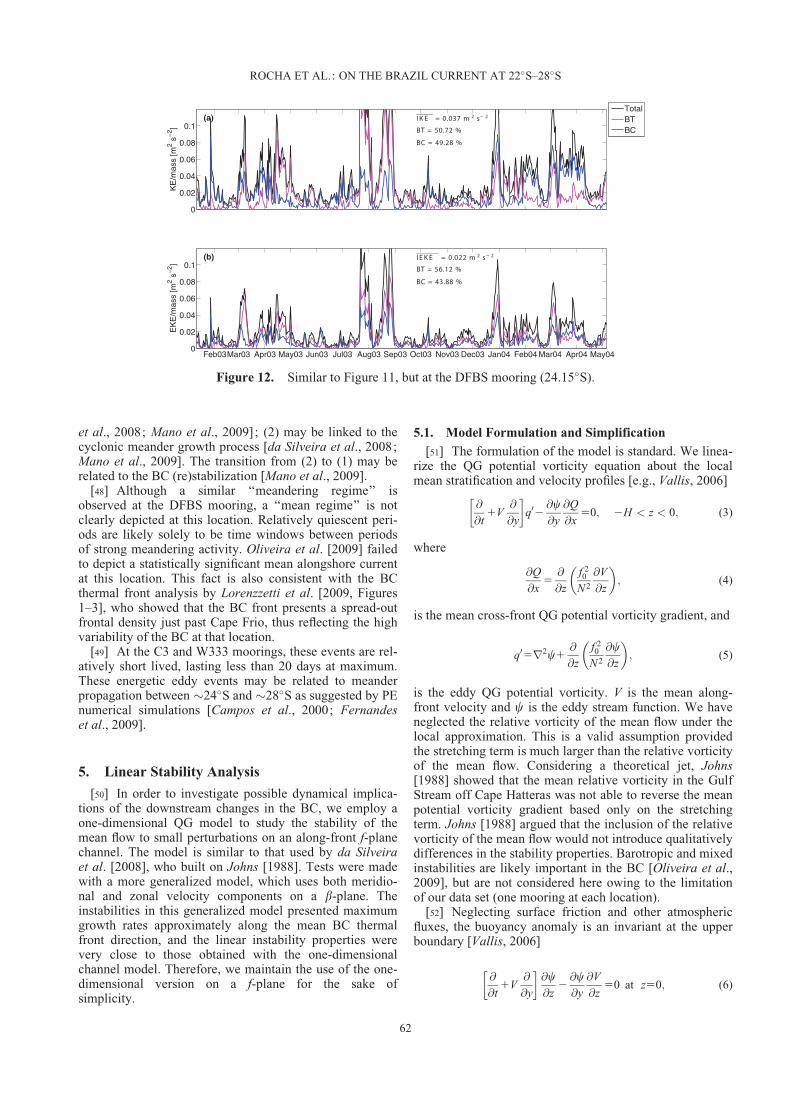
[40] First, we explore the time-mean values of IKE andIEKE, and their partition between barotropic and barocliniccomponents (Table 7). On average, the C3 mooringpresents the highest IKE level (0.045 m2 s22), followed bythe MARLIM mooring (0.038 m2 s22), the DFBS mooring(0.037 m2 s22), and the W333 mooring (0.032 m2 s22).However, as stated in section 2.2, this may be influencedby the relative distance of the moorings from the BC core;caution should be taken when comparing these results inabsolute values.

[41] An interesting result is the magnitude of the IEKEand its ratio to the IKE. On average, at the MARLIM moor-ing, the IEKE is estimated as 0.019 m2 s22, half the magni-tude of the IKE. High levels of IEKE are observed at theDFBS mooring (0.022 m2 s22), and its ratio to the IKE is�0.6. The C3 mooring presents a relatively weaker (butsubstantial) IEKE (0.014 m2 s22; its ratio to the IKE is�0.33. Farther south, at the W333 mooring, a similar levelof IEKE is found (0.014 m2 s22), though its ratio to theIKE is 0.44. Although these IEKE levels are generally lessthan those observed in the Gulf Stream and the Kuroshioregions [e.g., Wunsch, 1997], their relative importance tothe IKE is a remarkable feature of the BC off southeastBrazil. Thus, these results highlight (and in fact quantify)the importance of the mesoscale eddy field in the BC pathoff southeast Brazil, consistent with the previous studiesbased on quasi-synoptic observations [e.g., Campos et al.,1995], mooring data [da Silveira et al., 2008], surfacedrifters [Oliveira et al., 2009] and SST imagery analysis[Lorenzzetti et al., 2009]. In particular, these estimates sug-gest the dominance of the eddy field at the DFBS mooring.

[42] The SKE estimates are 0.113, 0.150, 0.163, and0.100 m2 s22 at the DFBS, MARLIM, C3, and W333,respectively. The SEKE/SKE ratios are 0.98, 0.64, 0.20,and 0.40 at the four moorings. Interestingly, at the DFBSand, to some extent, at the MARLIM mooring, the eddykinetic energy represents a greater fraction of the totalkinetic energy at the surface, consistent with the fact thatthe anomalies are very surface intensified at these locations[da Silveira et al., 2008, this study].

[43] It is difficult to compare absolute values of theseestimates against those of Oliveira et al. [2009]; while weestimate the SKE and SEKE in a single position, thoseauthors have taken averages of drifter-derived velocityover 0.5� 3 0.5� bins. Nonetheless, our results are in gen-eral agreement with those of the cited authors, specificallyin presenting high levels of SEKE at �22�S–23�S (their

Table 7. Time-Mean Water Column Average Kinetic Energy(IKEÞ and Eddy Kinetic Energy ðIEKEÞ, and Time-Mean Parti-tion of IKE and IEKE Between Barotropic and BaroclinicComponents

Mooring IKEðm2s22Þ BT (%) BC (%) IEKEðm2s22Þ BT (%) BC (%)

MARLIM 0.038 30.54 69.46 0.019 41.37 58.63DFBS 0.037 50.72 49.28 0.022 56.12 43.88C3 0.045 30.80 69.20 0.014 56.56 43.44W333 0.032 53.77 46.23 0.014 59.84 40.15


60

transects IV and V, close to the DFBS and MARLIM moor-ings, respectively) and relatively lower SEKE levels at�25�S and �28�S (their transects VI and VII, close to theC3 and W333 moorings, respectively).

4.3. Barotropic/Baroclinic Partition

[44] At the MARLIM mooring, on average, the IKE is70% baroclinic (mainly first mode); the IEKE is slightlymore barotropic (40%) than IKE. Based on synoptic directvelocity measurements, da Silveira et al. [2004] estimatethat the BC is 75–80% baroclinic, while da Silveira et al.[2008], using 152 days of the MARLIM series, indicatethat the along-front BC is 98% baroclinic. We emphasizethat our barotropic/baroclinic estimates are based on theIKE; as the cross-front component is mainly due to theeddy field, which is more barotropic, the partition will bemore barotropic than the estimates based only on thealong-isobath velocity component. Also, we appended thefirst 150 days of the MARLIM record, which is marked bystrong mesoscale activity, and likely contributes to thesediscrepancies. At the DFBS mooring, on average, a virtualequipartition between barotropic and baroclinic energy forthe total flow is observed, likely owing to the dominance ofthe eddy field. Indeed, the kinetic energy partition is almostthe same (�56% barotropic) for the velocity anomaly field.

[45] At the C3 mooring, on average, the total flowpresents a partition similar to that for the MARLIM moor-ing (�69% baroclinic). However, its eddy field seemsmuch more barotropic (�56%). In contrast, at the W333, adramatic change in the IKE partition is observed; the totalflow becomes �54% barotropic, confirming our qualitativeestimate based on the mean along-front velocity profiles(section 2.3). In this case, on average, the eddy field is justslightly more barotropic (�59%). While the relatively highbarotropicity of the total flow at the DFBS mooring is

likely due to the dominance of the eddy field over the meanflow [Oliveira et al., 2009, this study], this phenomenonseems to be a manifestation of the high barotropicity of themean flow itself at the W333 mooring (Figure 6).

4.4. Duration of Eddy Events

[46] The results presented in sections 4.2 and 4.3 repre-sent statistical estimates. However, the kinetic energy levelin a given day departs significantly from the time mean. Atthe MARLIM mooring, strong eddy events that occur at thebeginning of the series (April to May 1992) do not repeatin the end (Figure 11). These events are associated withreversals in the surface velocity vector in the BC domain(Figure 1). At the DFBS, C3, and W333 moorings (Figures12–14), strong energetic events seem to occur throughoutthe series; in that sense, the series are statistically morehomogeneous at these moorings. Typically, bursts ofenergy in the barotropic mode are associated with energeticeddy events at all moorings.

[47] At the MARLIM mooring, one such event lasts for�37 days (March to April 1992). Two similar long-livedbarotropic energy events are observed at the DFBS moor-ing, lasting �28 days (April to May 2003) and �32 days(August to September 2003). Indeed, these events aremarked by strong surface current vector reversals (Figures11 and 12). In particular, the event depicted at the MAR-LIM mooring contrasts with the latter 120 days of therecord, when the total flow is essentially baroclinic and lowlevels of IEKE are observed. Thus, there seems to be tworegimes at the MARLIM mooring: (1) a ‘‘mean regime’’(not perturbed), characterized by relatively low IEKE lev-els, and mainly baroclinic total flow; and (2) a ‘‘meander-ing regime’’ (perturbed), marked by high IEKE levels, andtherefore strongly barotropic total flow. In (1), the BC iswell defined and prone to baroclinic instability [da Silveira

0

0.02

0.04

0.06

0.08

0.1I K E = 0.038 m 2 s− 2

BT = 30.54 %

BC = 69.46 %

KE

/mas

s [m

2 s−

2 ]

(a)

TotalBTBC

Mar92 Apr92 May92 Jun92 Jul92 Aug92 Sep92 Oct92 Nov92 Dec920

0.02

0.04

0.06

0.08

0.1I E K E = 0.019 m 2 s− 2

BT = 41.37 %

BC = 58.63 %

(b)

EK

E/m

ass

[m2 s

−2 ]

Figure 11. Time series of water column average kinetic energy at the MARLIM mooring (22.7�S). (a)Total kinetic energy (KE). (b) Eddy kinetic energy (EKE). The fractions of energy (KE andEKE) in barotropic (bt) and baroclinic (bc) components are presented in magenta and blue, respectively.IKE ðIEKEÞ represents the average over time of IKE (IEKE). The temporal average of the percentage ofIKE and IEKE in barotropic and baroclinic components is also shown.


61

et al., 2008; Mano et al., 2009]; (2) may be linked to thecyclonic meander growth process [da Silveira et al., 2008;Mano et al., 2009]. The transition from (2) to (1) may berelated to the BC (re)stabilization [Mano et al., 2009].

[48] Although a similar ‘‘meandering regime’’ isobserved at the DFBS mooring, a ‘‘mean regime’’ is notclearly depicted at this location. Relatively quiescent peri-ods are likely solely to be time windows between periodsof strong meandering activity. Oliveira et al. [2009] failedto depict a statistically significant mean alongshore currentat this location. This fact is also consistent with the BCthermal front analysis by Lorenzzetti et al. [2009, Figures1–3], who showed that the BC front presents a spread-outfrontal density just past Cape Frio, thus reflecting the highvariability of the BC at that location.

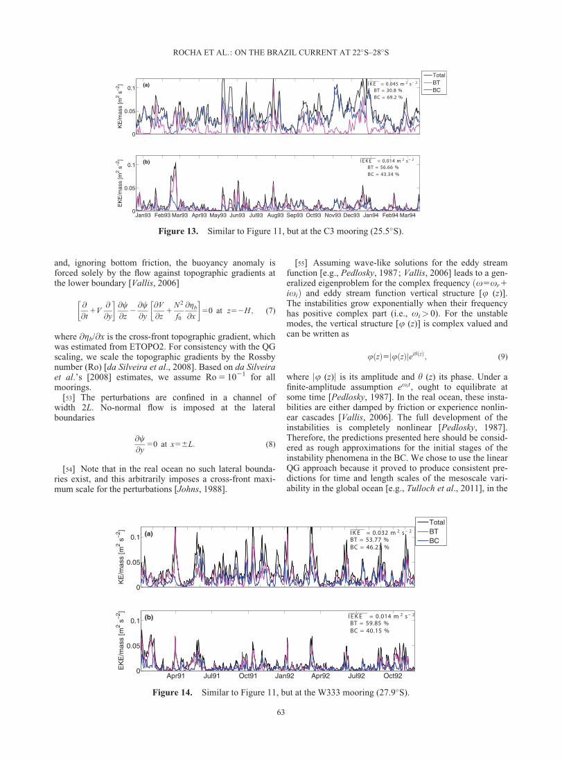
[49] At the C3 and W333 moorings, these events are rel-atively short lived, lasting less than 20 days at maximum.These energetic eddy events may be related to meanderpropagation between �24�S and �28�S as suggested by PEnumerical simulations [Campos et al., 2000; Fernandeset al., 2009].

5. Linear Stability Analysis

[50] In order to investigate possible dynamical implica-tions of the downstream changes in the BC, we employ aone-dimensional QG model to study the stability of themean flow to small perturbations on an along-front f-planechannel. The model is similar to that used by da Silveiraet al. [2008], who built on Johns [1988]. Tests were madewith a more generalized model, which uses both meridio-nal and zonal velocity components on a b-plane. Theinstabilities in this generalized model presented maximumgrowth rates approximately along the mean BC thermalfront direction, and the linear instability properties werevery close to those obtained with the one-dimensionalchannel model. Therefore, we maintain the use of the one-dimensional version on a f-plane for the sake ofsimplicity.

5.1. Model Formulation and Simplification

[51] The formulation of the model is standard. We linea-rize the QG potential vorticity equation about the localmean stratification and velocity profiles [e.g., Vallis, 2006]

@

@t1V

@

@y

� �q02

@w@y

@Q

@x50; 2H < z < 0; (3)

where

@Q

@x5@

@z

f 20

N 2

@V

@z

� �; (4)

is the mean cross-front QG potential vorticity gradient, and

q05r2w1@

@z

f 20

N2

@w@z

� �; (5)

is the eddy QG potential vorticity. V is the mean along-front velocity and w is the eddy stream function. We haveneglected the relative vorticity of the mean flow under thelocal approximation. This is a valid assumption providedthe stretching term is much larger than the relative vorticityof the mean flow. Considering a theoretical jet, Johns[1988] showed that the mean relative vorticity in the GulfStream off Cape Hatteras was not able to reverse the meanpotential vorticity gradient based only on the stretchingterm. Johns [1988] argued that the inclusion of the relativevorticity of the mean flow would not introduce qualitativelydifferences in the stability properties. Barotropic and mixedinstabilities are likely important in the BC [Oliveira et al.,2009], but are not considered here owing to the limitationof our data set (one mooring at each location).

[52] Neglecting surface friction and other atmosphericfluxes, the buoyancy anomaly is an invariant at the upperboundary [Vallis, 2006]

@

@t1V

@

@y

� �@w@z

2@w@y

@V

@z50 at z50; (6)

0

0.02

0.04

0.06

0.08

0.1I K E = 0.037 m 2 s− 2

BT = 50.72 %

BC = 49.28 %

(a)

KE

/mas

s [m

2 s−

2 ]

TotalBTBC

Feb03Mar03 Apr03 May03 Jun03 Jul03 Aug03 Sep03 Oct03 Nov03 Dec03 Jan04 Feb04 Mar04 Apr04 May040

0.02

0.04

0.06

0.08

0.1I E K E = 0.022 m 2 s− 2

BT = 56.12 %

BC = 43.88 %

(b)

EK

E/m

ass

[m2 s

−2 ]

Figure 12. Similar to Figure 11, but at the DFBS mooring (24.15�S).


62

and, ignoring bottom friction, the buoyancy anomaly isforced solely by the flow against topographic gradients atthe lower boundary [Vallis, 2006]

@

@t1V

@

@y

� �@w@z

2@w@y

@V

@z1

N 2

f0

@gb

@x

� �50 at z52H ; (7)

where @gb/@x is the cross-front topographic gradient, whichwas estimated from ETOPO2. For consistency with the QGscaling, we scale the topographic gradients by the Rossbynumber (Ro) [da Silveira et al., 2008]. Based on da Silveiraet al.’s [2008] estimates, we assume Ro 5 1021 for allmoorings.

[53] The perturbations are confined in a channel ofwidth 2L. No-normal flow is imposed at the lateralboundaries

@w@y

50 at x56L: (8)

[54] Note that in the real ocean no such lateral bounda-ries exist, and this arbitrarily imposes a cross-front maxi-mum scale for the perturbations [Johns, 1988].

[55] Assuming wave-like solutions for the eddy streamfunction [e.g., Pedlosky, 1987; Vallis, 2006] leads to a gen-eralized eigenproblem for the complex frequency ðx5xr1ixiÞ and eddy stream function vertical structure [u (z)].The instabilities grow exponentially when their frequencyhas positive complex part (i.e., xi> 0). For the unstablemodes, the vertical structure [u (z)] is complex valued andcan be written as

uðzÞ5juðzÞjeihðzÞ; (9)

where ju (z)j is its amplitude and h (z) its phase. Under afinite-amplitude assumption exit, ought to equilibrate atsome time [Pedlosky, 1987]. In the real ocean, these insta-bilities are either damped by friction or experience nonlin-ear cascades [Vallis, 2006]. The full development of theinstabilities is completely nonlinear [Pedlosky, 1987].Therefore, the predictions presented here should be consid-ered as rough approximations for the initial stages of theinstability phenomena in the BC. We chose to use the linearQG approach because it proved to produce consistent pre-dictions for time and length scales of the mesoscale vari-ability in the global ocean [e.g., Tulloch et al., 2011], in the

0

0.05

0.1I K E = 0.032 m 2 s− 2

BT = 53.77 %BC = 46.23 %

(a)

KE

/mas

s [m

2 s−

2 ]

TotalBTBC

Apr91 Jul91 Oct91 Jan92 Apr92 Jul92 Oct920

0.05

0.1I E K E = 0.014 m 2 s− 2

BT = 59.85 %BC = 40.15 %

(b)

EK

E/m

ass

[m2 s

−2 ]

Figure 14. Similar to Figure 11, but at the W333 mooring (27.9�S).

0

0.05

0.1I K E = 0.045 m 2 s− 2

BT = 30.8 %BC = 69.2 %

(a)

KE

/mas

s [m

2 s−

2 ]

TotalBTBC

Jan93 Feb93 Mar93 Apr93 May93 Jun93 Jul93 Aug93 Sep93 Oct93 Nov93 Dec93 Jan94 Feb94 Mar940

0.05

0.1I E K E = 0.014 m 2 s− 2

BT = 56.66 %BC = 43.34 %

(b)

EK

E/m

ass

[m2 s

−2 ]

Figure 13. Similar to Figure 11, but at the C3 mooring (25.5�S).


63

Gulf Stream off Cape Hatteras [Johns, 1988] and in the BCSystem within the Campos Basin [da Silveira et al., 2008].

[56] For each mooring, the eigenproblem is solvednumerically for a range of wavelengths spanning 10–1000km. Similarly to da Silveira et al. [2008], we use the meanalong-front velocity profile synthesized using the dynami-cal modes (section 2.3; Figure 6). As the mean along frontat the DFBS mooring presents low statistical significance,the stability analysis at this location would be very inaccu-rate. Therefore, we perform the stability analysis only forthe MARLIM, C3, and W333 moorings. The mean stratifi-cation is taken as the climatological profile (Figure 15a).

[57] We set L 5 100 km which represents the averagewidth of the BC [da Silveira et al., 2008]. Tests for differ-ent Ls were performed. The results proved insensitive tovalues greater than 100 km in agreement with Johns[1988].

5.2. Necessary Conditions for Baroclinic Instability

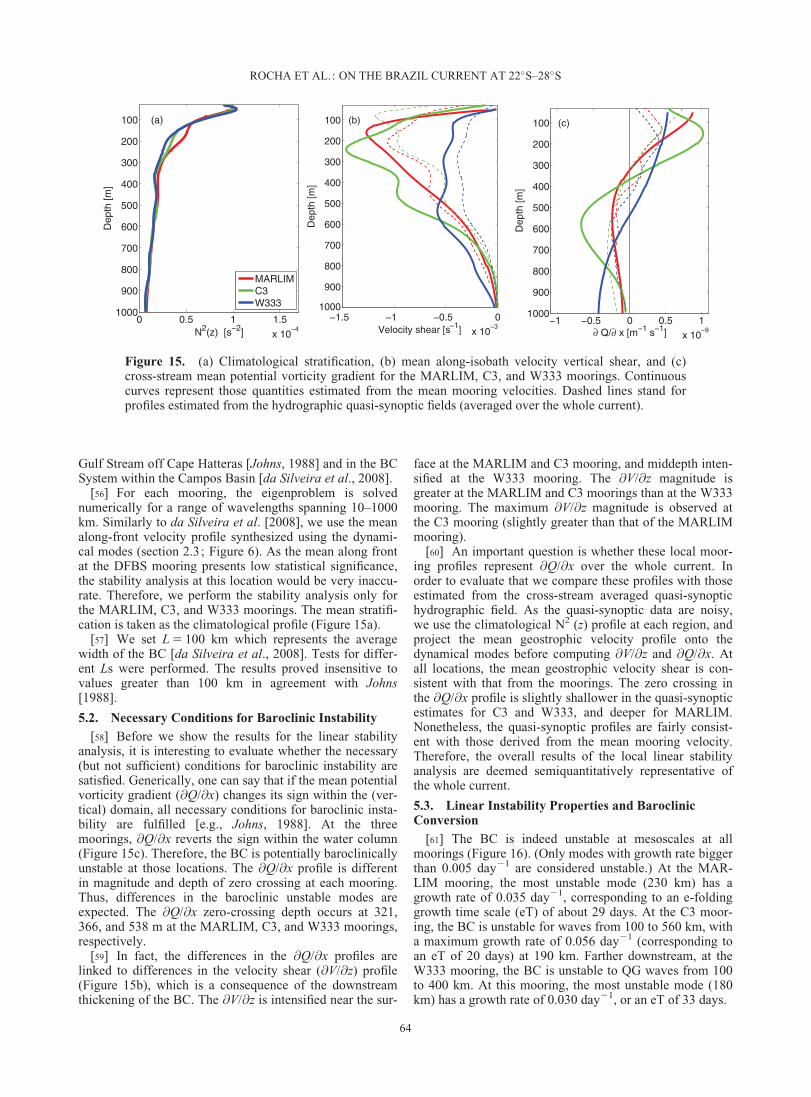
[58] Before we show the results for the linear stabilityanalysis, it is interesting to evaluate whether the necessary(but not sufficient) conditions for baroclinic instability aresatisfied. Generically, one can say that if the mean potentialvorticity gradient (@Q/@x) changes its sign within the (ver-tical) domain, all necessary conditions for baroclinic insta-bility are fulfilled [e.g., Johns, 1988]. At the threemoorings, @Q/@x reverts the sign within the water column(Figure 15c). Therefore, the BC is potentially baroclinicallyunstable at those locations. The @Q/@x profile is differentin magnitude and depth of zero crossing at each mooring.Thus, differences in the baroclinic unstable modes areexpected. The @Q/@x zero-crossing depth occurs at 321,366, and 538 m at the MARLIM, C3, and W333 moorings,respectively.

[59] In fact, the differences in the @Q/@x profiles arelinked to differences in the velocity shear (@V/@z) profile(Figure 15b), which is a consequence of the downstreamthickening of the BC. The @V/@z is intensified near the sur-

face at the MARLIM and C3 mooring, and middepth inten-sified at the W333 mooring. The @V/@z magnitude isgreater at the MARLIM and C3 moorings than at the W333mooring. The maximum @V/@z magnitude is observed atthe C3 mooring (slightly greater than that of the MARLIMmooring).

[60] An important question is whether these local moor-ing profiles represent @Q/@x over the whole current. Inorder to evaluate that we compare these profiles with thoseestimated from the cross-stream averaged quasi-synoptichydrographic field. As the quasi-synoptic data are noisy,we use the climatological N2 (z) profile at each region, andproject the mean geostrophic velocity profile onto thedynamical modes before computing @V/@z and @Q/@x. Atall locations, the mean geostrophic velocity shear is con-sistent with that from the moorings. The zero crossing inthe @Q/@x profile is slightly shallower in the quasi-synopticestimates for C3 and W333, and deeper for MARLIM.Nonetheless, the quasi-synoptic profiles are fairly consist-ent with those derived from the mean mooring velocity.Therefore, the overall results of the local linear stabilityanalysis are deemed semiquantitatively representative ofthe whole current.

5.3. Linear Instability Properties and BaroclinicConversion

[61] The BC is indeed unstable at mesoscales at allmoorings (Figure 16). (Only modes with growth rate biggerthan 0.005 day21 are considered unstable.) At the MAR-LIM mooring, the most unstable mode (230 km) has agrowth rate of 0.035 day21, corresponding to an e-foldinggrowth time scale (eT) of about 29 days. At the C3 moor-ing, the BC is unstable for waves from 100 to 560 km, witha maximum growth rate of 0.056 day21 (corresponding toan eT of 20 days) at 190 km. Farther downstream, at theW333 mooring, the BC is unstable to QG waves from 100to 400 km. At this mooring, the most unstable mode (180km) has a growth rate of 0.030 day21, or an eT of 33 days.

0 0.5 1 1.5

x 10−4

1000

900

800

700

600

500

400

300

200

100

N2(z) [s−2]

Dep

th [m

]

(a)

MARLIMC3W333

−1.5 −1 −0.5 0

x 10−3

1000

900

800

700

600

500

400

300

200

100 (b)

Velocity shear [s−1]

Dep

th [m

]−1 −0.5 0 0.5 1

x 10−9

1000

900

800

700

600

500

400

300

200

100 (c)

∂ Q/∂ x [m−1 s−1]

Dep

th [m

]

Figure 15. (a) Climatological stratification, (b) mean along-isobath velocity vertical shear, and (c)cross-stream mean potential vorticity gradient for the MARLIM, C3, and W333 moorings. Continuouscurves represent those quantities estimated from the mean mooring velocities. Dashed lines stand forprofiles estimated from the hydrographic quasi-synoptic fields (averaged over the whole current).


64

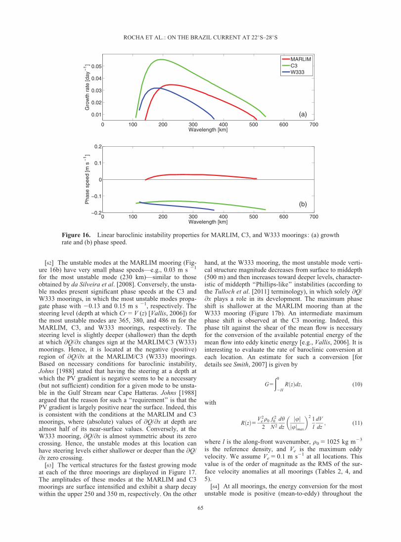
[62] The unstable modes at the MARLIM mooring (Fig-ure 16b) have very small phase speeds—e.g., 0.03 m s 21

for the most unstable mode (230 km)—similar to thoseobtained by da Silveira et al. [2008]. Conversely, the unsta-ble modes present significant phase speeds at the C3 andW333 moorings, in which the most unstable modes propa-gate phase with 20.13 and 0.15 m s 21, respectively. Thesteering level (depth at which Cr 5 V (z) [Vallis, 2006]) forthe most unstable modes are 365, 380, and 486 m for theMARLIM, C3, and W333 moorings, respectively. Thesteering level is slightly deeper (shallower) than the depthat which @Q/@x changes sign at the MARLIM/C3 (W333)moorings. Hence, it is located at the negative (positive)region of @Q/@x at the MARLIM/C3 (W333) moorings.Based on necessary conditions for baroclinic instability,Johns [1988] stated that having the steering at a depth atwhich the PV gradient is negative seems to be a necessary(but not sufficient) condition for a given mode to be unsta-ble in the Gulf Stream near Cape Hatteras. Johns [1988]argued that the reason for such a ‘‘requirement’’ is that thePV gradient is largely positive near the surface. Indeed, thisis consistent with the conditions at the MARLIM and C3moorings, where (absolute) values of @Q/@x at depth arealmost half of its near-surface values. Conversely, at theW333 mooring, @Q/@x is almost symmetric about its zerocrossing. Hence, the unstable modes at this location canhave steering levels either shallower or deeper than the @Q/@x zero crossing.

[63] The vertical structures for the fastest growing modeat each of the three moorings are displayed in Figure 17.The amplitudes of these modes at the MARLIM and C3moorings are surface intensified and exhibit a sharp decaywithin the upper 250 and 350 m, respectively. On the other

hand, at the W333 mooring, the most unstable mode verti-cal structure magnitude decreases from surface to middepth(500 m) and then increases toward deeper levels, character-istic of middepth ‘‘Phillips-like’’ instabilities (according tothe Tulloch et al. [2011] terminology), in which solely @Q/@x plays a role in its development. The maximum phaseshift is shallower at the MARLIM mooring than at theW333 mooring (Figure 17b). An intermediate maximumphase shift is observed at the C3 mooring. Indeed, thisphase tilt against the shear of the mean flow is necessaryfor the conversion of the available potential energy of themean flow into eddy kinetic energy [e.g., Vallis, 2006]. It isinteresting to evaluate the rate of baroclinic conversion ateach location. An estimate for such a conversion [fordetails see Smith, 2007] is given by

G5

ð0

2HRðzÞdz; (10)

with

RðzÞ5 V 2e q0

2

f 20

N2

dhdz

jujjujmax

� �2 1

l

dV

dz; (11)

where l is the along-front wavenumber, q0 5 1025 kg m23

is the reference density, and Ve is the maximum eddyvelocity. We assume Ve 5 0.1 m s21 at all locations. Thisvalue is of the order of magnitude as the RMS of the sur-face velocity anomalies at all moorings (Tables 2, 4, and5).

[64] At all moorings, the energy conversion for the mostunstable mode is positive (mean-to-eddy) throughout the

0 100 200 300 400 500 600 700

0.01

0.02

0.03

0.04

0.05

(a)

Wavelength [km]

Gro

wth

rat

e [d

ay−

1]

MARLIMC3W333

0 100 200 300 400 500 600 700−0.2

−0.1

0

0.1

0.2

(b)

Wavelength [km]

Pha

se s

peed

[m s

−1]

Figure 16. Linear baroclinic instability properties for MARLIM, C3, and W333 moorings: (a) growthrate and (b) phase speed.


65

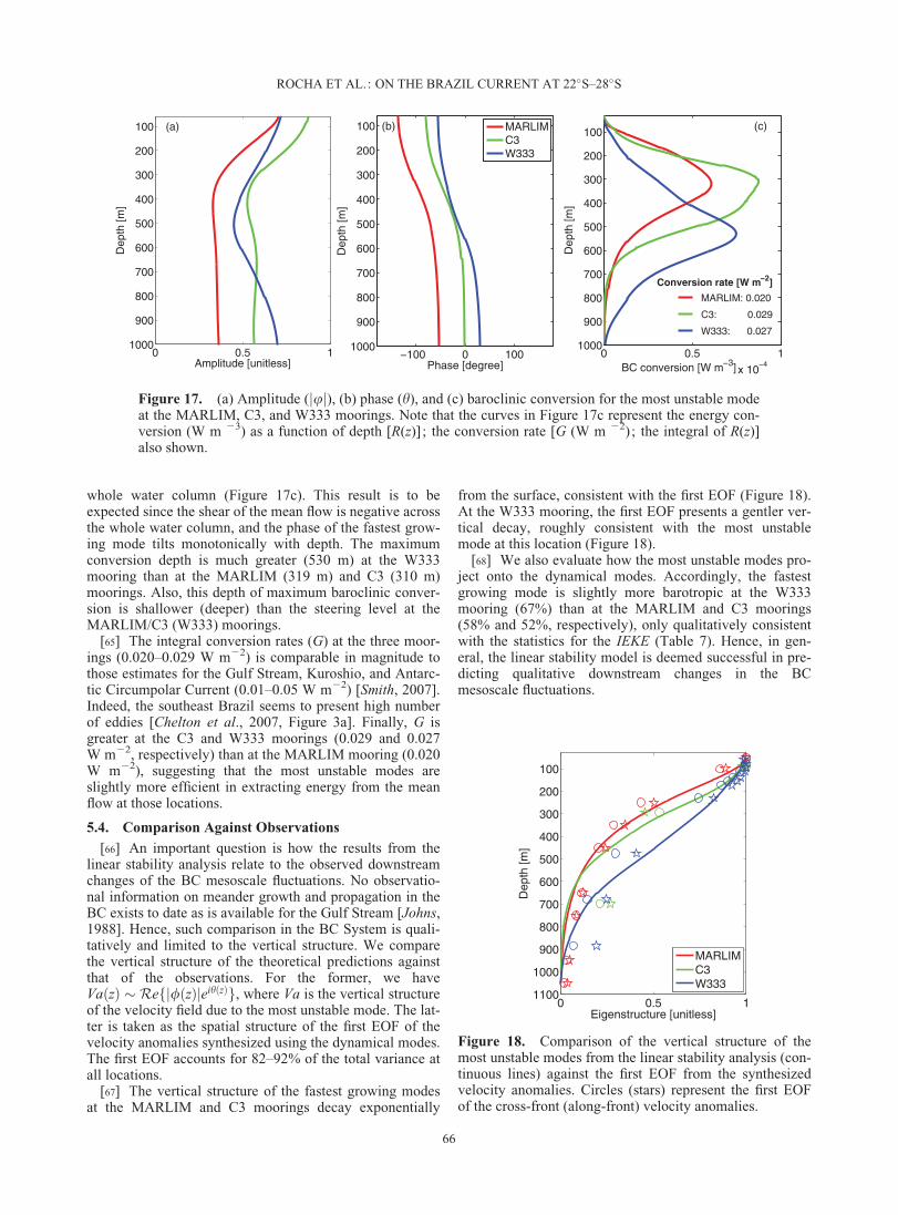
whole water column (Figure 17c). This result is to beexpected since the shear of the mean flow is negative acrossthe whole water column, and the phase of the fastest grow-ing mode tilts monotonically with depth. The maximumconversion depth is much greater (530 m) at the W333mooring than at the MARLIM (319 m) and C3 (310 m)moorings. Also, this depth of maximum baroclinic conver-sion is shallower (deeper) than the steering level at theMARLIM/C3 (W333) moorings.

[65] The integral conversion rates (G) at the three moor-ings (0.020–0.029 W m22) is comparable in magnitude tothose estimates for the Gulf Stream, Kuroshio, and Antarc-tic Circumpolar Current (0.01–0.05 W m22) [Smith, 2007].Indeed, the southeast Brazil seems to present high numberof eddies [Chelton et al., 2007, Figure 3a]. Finally, G isgreater at the C3 and W333 moorings (0.029 and 0.027W m22, respectively) than at the MARLIM mooring (0.020W m22), suggesting that the most unstable modes areslightly more efficient in extracting energy from the meanflow at those locations.

5.4. Comparison Against Observations

[66] An important question is how the results from thelinear stability analysis relate to the observed downstreamchanges of the BC mesoscale fluctuations. No observatio-nal information on meander growth and propagation in theBC exists to date as is available for the Gulf Stream [Johns,1988]. Hence, such comparison in the BC System is quali-tatively and limited to the vertical structure. We comparethe vertical structure of the theoretical predictions againstthat of the observations. For the former, we haveVaðzÞ � Refj/ðzÞjeihðzÞg, where Va is the vertical structureof the velocity field due to the most unstable mode. The lat-ter is taken as the spatial structure of the first EOF of thevelocity anomalies synthesized using the dynamical modes.The first EOF accounts for 82–92% of the total variance atall locations.

[67] The vertical structure of the fastest growing modesat the MARLIM and C3 moorings decay exponentially

from the surface, consistent with the first EOF (Figure 18).At the W333 mooring, the first EOF presents a gentler ver-tical decay, roughly consistent with the most unstablemode at this location (Figure 18).

[68] We also evaluate how the most unstable modes pro-ject onto the dynamical modes. Accordingly, the fastestgrowing mode is slightly more barotropic at the W333mooring (67%) than at the MARLIM and C3 moorings(58% and 52%, respectively), only qualitatively consistentwith the statistics for the IEKE (Table 7). Hence, in gen-eral, the linear stability model is deemed successful in pre-dicting qualitative downstream changes in the BCmesoscale fluctuations.

0 0.5 11000

900

800

700

600

500

400

300

200

100 (a)

Amplitude [unitless]

Dep

th [m

]

−100 0 1001000

900

800

700

600

500

400

300

200

100 (b)

Phase [degree]

Dep

th [m

]

MARLIMC3W333

0 0.5 1

x 10−4

1000

900

800

700

600

500

400

300

200

100 (c)

Conversion rate [W m−2]

MARLIM: 0.020

C3: 0.029

W333: 0.027

BC conversion [W m−3]

Dep

th [m

]

Figure 17. (a) Amplitude (juj), (b) phase (h), and (c) baroclinic conversion for the most unstable modeat the MARLIM, C3, and W333 moorings. Note that the curves in Figure 17c represent the energy con-version (W m 23) as a function of depth [R(z)] ; the conversion rate [G (W m 22); the integral of R(z)]also shown.

0 0.5 11100

1000

900

800

700

600

500

400

300

200

100

Eigenstructure [unitless]

Dep

th [m

]

MARLIMC3W333

Figure 18. Comparison of the vertical structure of themost unstable modes from the linear stability analysis (con-tinuous lines) against the first EOF from the synthesizedvelocity anomalies. Circles (stars) represent the first EOFof the cross-front (along-front) velocity anomalies.


66

6. Summary and Discussion

[69] The goal of the present work is to investigate thedownstream changes in the BC as it flows off southeastBrazil (22�S–28�S). We analyze four current meter moor-ing records spanning this region, namely the MARLIM(22.7�S), DFBS (24.15�S), C3 (25.5�S), and W333(27.9�S). The mooring data depict the downstream growthin vertical extension of BC. The 350 m deep flow at theMARLIM mooring becomes an 850 m deep flow at theW333 mooring; an intermediate scenario is observed at theC3 mooring, namely a 550 m deep BC. At the DFBS moor-ing, the mean BC extends down to 400 m, although themean estimate at this location has low statistical signifi-cance owing to the high variability. At the MARLIM moor-ing, the BC is also highly variable, presenting a standarddeviation that exceeds the mean at the uppermost instru-ment. Conversely, northeastward flowing IWBC provedmuch less variable at the MARLIM mooring. Fartherdownstream, the entire water column over the slope seemsto flow to the southeast. Therefore, the Santos bifurcationseems to occur somewhere between 25.5�S and 27.9�S,consistent with a recent description on the basis of float tra-jectories [Legeais et al., 2013].

[70] Quasi-synoptic observations contemporary with themooring records are generally consistent with the scenariothat emerges from the mean moored velocity analysis. Geo-strophic estimates reveal that the BC transport presents amajor increase from the C3 mooring (5.73 Sv) to the W333mooring (10.02 Sv). Part of this increment is certainly asso-ciated with the Santos bifurcation. The presence of a recir-culation feeding the BC at about 27�–28�S is not ruled out[Peterson and Stramma, 1991; Stramma and England,1999], and may account for a fraction of this transportgrowth. Furthermore, variabilities of the BC transport onmany time scales between the two hydrographic sectionoccupations (�7 months) can contribute to thesedifferences.

[71] The water column average kinetic energy (IKE) andits barotropic/baroclinic partition estimates reveal that thechanges in the BC System vertical structure are accompa-nied by strong changes in the vertical partition of the IKE.Accordingly, the BC is, on average, highly baroclinic(�70%) at the MARLIM mooring, in agreement with pre-vious estimates [da Silveira et al., 2004] that point the highbaroclinicity of the BC System close to this latitude; simi-lar results are obtained at the C3 mooring. A significantchange in the partition of the energy is observed to thesouth of the C3 mooring. The total flow becomes 54% bar-otropic at the W333 mooring.

[72] The water column average eddy kinetic energy(IEKE) and its ratio to the IKE confirms the importance ofthe BC mesoscale activity as it flows off the southeast : theIEKE accounts for from 33% (W333 mooring) to 60%(DFBS mooring) of the IKE. This fact is indeed in agree-ment with quasi-synoptic observations [e.g., Campos et al.,1995, 2000; da Silveira et al., 2004], drifter statistics [Oli-veira et al., 2009] and thermal front analysis [Lorenzzettiet al., 2009]. Moreover, our analysis suggests that the eddyfield dominates the mean flow at the DFBS mooring. TheIEKE is, on average, more barotropic than the IKE. Theexception is the W333 mooring, where the IEKE has

approximate the same energy partition as the total flow(�59% barotropic).

[73] Indeed, the analysis of the IKE and IEKE timeseries reveals that these eddy events are associated withbursts of energy in the barotropic mode, thus supportingthe idea that the BC meanders are more barotropic than themean flow [da Silveira et al., 2008]. At the MARLIMmooring, the persistence of the energy in the barotropicmode for �37 days may be an indication of a quasi-standing meander growth in the region [da Silveira et al.,2008; Mano et al., 2009]. Similar long-lived eddy eventsare observed at the DFBS mooring. Conversely, at the C3mooring, these bursts of energy in the barotropic mode last20 days at maximum (typically much less), likely owing tomeander propagation [Campos et al., 2000; Fernandeset al., 2009].

[74] We also evaluate the stability of the mean along-front BC to small-amplitude perturbations at the moorings.As far as the baroclinic instability is concerned, the BCdownstream vertical extension growth has two majoreffects on the linear instability properties. First, the unsta-ble waves are slightly but noticeably shorter (�20%) to thesouth. The estimated fastest growing modes were associ-ated with wavelengths of 230, 190, and 180 km, at theMARLIM, C3, and W333 moorings, respectively. Second,the unstable waves at the MARLIM mooring present verysmall phase speeds (�0.03 m s21), whereas those at the C3and W333 moorings have significant propagation speeds(20.13 and 20.15 m s21, respectively). These predictionsare qualitatively consistent with SST imagery analysis[Garfield, 1990] and PE simulations [Campos et al., 2000;Fernandes et al., 2009]. The theoretical prediction that thevorticity waves are shorter to the south still needs evidencefrom observations.

[75] The fastest growing modes have vertical structuresthat resemble the first EOF of the observed velocity anoma-lies. These modes present rates of baroclinic conversioncomparable to those observed in the other strong currents[Smith, 2007]. This is consistent with the fact that the IEKEis significant at all moorings. The most unstable modes atthe W333 and C3 moorings are more efficient in transfer-ring energy from the mean flow than the fastest growingmode at the MARLIM mooring. This apparently contra-dicts the fact that the IEKE accounts for a larger fraction ofthe IKE at the MARLIM mooring (0.5) than at the W333and C3 moorings (0.44 and 0.3, respectively). However, ininterpreting this result, one should bear in mind that thisprediction only suggests that a given perturbation wouldgrow more efficiently at the expense of the mean flow atthe W333 and C3 moorings. It does not indicate that thereare more perturbations at these locations, which may beaccounted for by, e.g., local differences in topography andchanges in the continental margin orientation [Camposet al., 1995].

7. Final Remarks

[76] We conclude by answering the questions posed insection 1: (1a) The BC thickens from a 350 m at 22.7�S to850 m at 27.9�S; (1b) Hydrographic observations suggestthat the BC transport is increased by at least 4.3 Sv from25.5�S to 27.9�S. (2a and 2b) The total flow is mainly


67

baroclinic (�70%) at 22.7�S and 25.5�S, and is mainly bar-otropic at (�54%) at 27.9�S; it should be noted that anequipartition is observed for the total flow at 24.15�S,likely a manifestation of the dominance of the eddy field atthis location. (3) In a water column average sense, the eddyfield accounts for 30–60% of the total kinetic energy. (4a)The changes are twofold: (i) The fastest growing modesare shorter to the south (at 25.5�S and 27.9�S); (ii) at25.5�S and 27.9�S, these unstable waves tend propagate tothe south, as opposed to quasi-standing waves at 22.7�S.(4b) These modes have vertical structures roughly consist-ent with the observed mesoscale fluctuations.

[77] The most vexing limitation of this paper is that wewere not able to quantitatively assess the linear stabilitypredictions owing to lack of information on the BC. Futureobservational programs should focus on obtaining measure-ments to estimate of growth rates and propagation speedsof the BC meanders, e.g., by using inverted echo sounderarrays [e.g., Watts and Johns, 1982]. One could obtainempirical dispersion relationships; theories could then bequantitatively tested against these estimates.

[78] Finally, barotropic conversions seem to be impor-tant along the entire BC path [Oliveira et al., 2009]. Oneimportant open question concerns the relative importanceof the baroclinic and barotropic instability in giving rise tothe mesoscale variability of the BC. The full instability pro-cess cannot be accounted for by linear models. Therefore,this question should be assessed by combining observations[e.g., da Silveira et al., 2008] and primitive-equation (PE)numerical models [e.g., Mano et al., 2009]. However, PEmodels are expected to be consistent with the available sta-tistics for the BC [e.g., Oliveira et al., 2009]. We believethat the present estimates could also provide a test bed forthose models.

[79] Acknowledgments. We acknowledge three anonymousreviewers for their thorough comments that substantially improved thispaper. We also thank E.D. Barton (Editor in chief, JGR-Oceans), AmitTandon (UMassD), Jos�e Roberto B. Leite (IOUSP), Jos�e Luiz L. de Aze-vedo (FURG), Marcelo Dottori (IOUSP), Rick Salmon (SIO), Frank‘‘Chico’’ Smith (UMassD), and Janet Sprintall (SIO) for useful comments,insights, and editorial assistance. The COROAS HM2 data were kindlyprovided by Edmo Campos (IOUSP). We are also grateful to Petr�oleo Bra-sileiro S. A.—PETROBRAS for providing the MARLIM data set and pro-moting oceanographic research projects. This research was funded by S~aoPaulo Research Foundation (FAPESP 2010/13629-6, 2012/02119-2 and2008/58101-9). ICAS and BMC acknowledge support from CNPq(307122/2010-7).

ReferencesAntonov, J. I., D. Seidov, T. P. Boyer, R. A. Locarnini, A. V. Mishonov, H.

E. Garcia, O. K. Baranova, M. M. Zweng, and D. R. Johnson (2010),NOAA Atlas NESDIS 68 WORLD OCEAN ATLAS 2009, vol. 2: Salin-ity, technical report. march, U.S. Gov. Print. Off., Washington, D. C.

Beckers, J. M., and M. Rixen (2003), EOF calculations and data fillingfrom incomplete oceanographic datasets, J. Atmos. Oceanic Technol.,20(12), 1839–1856.

Böebel, O., R. E. Davis, M. Ollitraut, R. G. Peterson, P. L. Richard, C.Schmid, and W. Zenk (1999), The intermediate depth circulation of thewestern South Atlantic, Geophys. Res. Lett., 26(21), 3329–3332.

Campos, E. J. D., J. E. Goncalves, and Y. Ikeda (1995), Water mass struc-ture and geostrophic circulation in the South Brazil Bight—Summer of1991, J. Geophys. Res., 100(C9), 253–250.

Campos, E. J. D., Y. Ikeda, B. M. Castro, S. A. Gaeta, J. A. Lorenzetti, andR. Stevenson (1996), Experiment studies circulation in the WesternSouth Atlantic, EOS Trans. AGU, 77(27), 253–250.

Campos, E. J. D., D. Velhote, and I. C. A. Silveira (2000), Shelf breakupwelling driven by Brazil Current cyclonic meanders, Geophys. Res.Lett., 27(6), 751–754.

Chelton, D. B., M. G. Schlax, R. M. Samelson, and R. A. de Szoeke (2007),Global observations of large oceanic eddies, Geophys. Res. Lett., 34,L15605, doi:10.1029/2007GL030812.

da Silveira, I. C. A., A. C. K. Schmidt, E. J. D. Campos, S. S. Godoi, and Y.Ikeda (2000), A Corrente do Brasil ao Largo da Costa Leste brasileira,Rev. Bras. Oceanogr., 48(2), 171–183.

da Silveira, I. C. A., L. Calado, B. M. Castro, M. Cirano, J. A. M. Lima,and A. D. S. Mascarenhas (2004), On the baroclinic structure of the Bra-zil Current intermediate western boundary current system at 2223S, Geo-phys. Res. Lett., 31, L14308, doi:10.1029/2004GL020036.

da Silveira, I. C. A., J. A. M. Lima, A. C. K. Schmidt, W. Ceccopieri, A.Sartori, C. P. F. Franscisco, and R. F. C. Fontes (2008), Is the meandergrowth in the Brazil Current system off Southeast Brazil due to baro-clinic instability?, Dyn. Atmos. Oceans, 45(3–4), 187–207, doi:10.1016/j.dynatmoce.2008.01.002.

Dengler, M., F. A. Schott, C. Eden, P. Brandtl, and R. Zantopp (2004),Break-up of the Atlantic deep western boundary current into eddies at8�S, Nature, 432, 1018–1020.

Emery, W., and R. Thomson (2001), Data Analysis Methods in PhysicalOceanography, Elsevier, Amsterdam, the Netherlands.

Evans, D., and S. R. Signorini (1985), Vertical structure of the Brazil Cur-rent, Nature, 315, 48–50.

Fernandes, A. M., I. C. da Silveira, L. Calado, E. J. Campos, and A. M.Paiva (2009), A two-layer approximation to the Brazil Current interme-diate western boundary current system between 20�S and 28�S, OceanModel., 29(2), 154–158, doi:10.1016/j.ocemod.2009.03.008.

Garfield, N. (1990), The Brazil Current at subtropical latitudes, PhD thesis,Univ. of Rhode Island, Kingston.

Glover, D. M., W. J. Jenkins, and S. C. Doney (2011), Modeling Methodsfor Marine Science, Cambridge Univ. Press, Cambridge, U. K.

Johns, W. E. (1988), One-dimensional baroclinically unstable waves on theGulf Stream potential vorticity gradient near Cape Hatteras, Dyn. Atmos.Oceans, 11, 323–350.

Legeais, J.-F., M. Ollitrault, and M. Arhan (2013), Lagrangian observationsin the intermediate western boundary current of the South Atlantic, DeepSea Res., Part II, 85, 109–126, doi:10.1016/j.dsr2.2012.07.028.

Locarnini, R. A., A. V. Mishonov, J. I. Antonov, T. P. Boyer, H. E. Garcia,O. K. Baranova, M. M. Zweng, and D. R. Johnson (2010), NOAA AtlasNESDIS 68 WORLD OCEAN ATLAS 2009, vol. 1: Temperature, tech-nical report march, U.S. Gov. Print. Off., Washington, D. C.

Lorenzzetti, J. A., J. L. Stech, W. L. M. Filho, and A. T. Assireu (2009),Satellite observation of Brazil Current inshore thermal front in the SWSouth Atlantic: Space/time variability and sea surface temperatures,Cont. Shelf Res., 29, 2061–2068.

Mano, M. F., A. M. Paiva, A. R. Torres Jr., and A. L. G. A. Coutinho(2009), Energy flux to a cyclonic eddy off Cabo Frio, Brazil, J. Phys.Oceanogr., 39, 2999–3010, doi:10.1175/2009JPO4026.1.

M€uller, T. J., Y. Ikeda, N. Zangenberg, and L. V. Nonato (1998), Directmeasurements of western boundary currents off Brazil between 20�S and28�S, J. Geophys. Res., 103(C3), 5429–5437.

Oliveira, L. R., A. R. Piola, M. M. Mata, and I. D. Soares (2009), BrazilCurrent surface circulation and energetics observed from drifting buoys,J. Geophys. Res., 114, C10006, doi:10.1029/2008JC004900.

Pedlosky, J. (1987), Geophysical Fluid Dynamics, Springer study ed.,Springer, New York.

Peterson, R. G., and L. Stramma (1991), Upper-level circulation in theSouth Atlantic Ocean, Prog. Oceanogr., 26, 1–73.

Schott, F. A., M. Dengler, R. Zantopp, L. Stramma, J. Fisher, and P. Brandt(2005), The shallow and deep western boundary current circulation ofthe South Atlantic at 5�S–11�S, J. Phys. Oceanogr., 35, 2031–2053.

Smith, K. S. (2007), The geography of linear baroclinic instability inEarth’s oceans, J. Mar. Res., 65, 655–683.

Stramma, L., and M. England (1999), On the water masses and mean circu-lation of the south Atlantic ocean, J. Geophys. Res., 104(C9), 20,863–20,883.

Stramma, L., J. Fischer, and J. Reppin (1995), The North Brazil Undercur-rent, Deep Sea Res., Part I, 42(5), 773–795, doi:10.1016/0967-0637(95)00014-W.

Szuts, Z. B., J. R. Blundell, M. P. Chidichimo, and J. Marotzke (2012), Avertical-mode decomposition to investigate low-frequency internalmotion across the Atlantic at 26 N, Ocean Sci., 8(3), 345–367, doi:10.5194/os-8-345-2012.


68

info:doi/10.1029/2007GL030812

info:doi/10.1029/2004GL020036

info:doi/10.1016/j.dynatmoce.2008.01.002

info:doi/10.1016/j.dynatmoce.2008.01.002

info:doi/10.1016/j.ocemod.2009.03.008

info:doi/10.1016/j.dsr2.2012.07.028

info:doi/10.1175/2009JPO4026.1

info:doi/10.1029/2008JC004900

info:doi/10.1016/0967-0637(95)00014-W

info:doi/10.1016/0967-0637(95)00014-W

info:doi/10.5194/os-8-345-2012

Tulloch, R., J. Marshall, C. Hill, and K. S. Smith (2011), Scales, growthrates, and spectral fluxes of baroclinic instability in the ocean, J. Phys.Oceanogr., 41, 1057–1575.

Vallis, G. K. (2006), Atmospheric and Oceanic Fluid Dynamics, 745 pp.,Cambridge Univ. Press, Cambridge, U. K.

Watts, D. R., and W. E. Johns (1982), Gulf stream meanders: Observationson propagation and growth, J. Geophys. Res., 87(C12), 9467–9476, doi:10.1029/JC087iC12p09467.

Wunsch, C. (1997), The vertical partition of oceanic horizontal kineticenergy, J. Phys. Oceanogr., 27(1), 1770–1794.


69

info:doi/10.1029/JC087iC12p09467

Documents

Vertical structure, energetics, and dynamics of the Brazil Current System at 22°S-28°S