Vertical modeling: analysis of competingrisks data with a cure proportion

M. A. Nicolaiea ∗ and J.M.G. Taylorb and C. Legranda

a Institute of Statistics, Biostatistics and Actuarial Sciences, Catholic University of Louvain,

Voie du Roman Pays 20, bte L1.04.01, 1348 Louvain-la-Neuve, Belgiumb School of Public Health, University of Michigan, M4509 SPH II, 1415 Washington Heights,

Ann Arbor, Michigan 48109-2029, USA

March 27, 2018

Abstract

In this paper, we extend the vertical modeling approach for the analysis ofsurvival data with competing risks to incorporate a cured fraction in the population,that is, a proportion of the population for which none of the competing events canoccur. The proposed method has three components: the proportion of cure, therisk of failure, irrespective of the cause, and the relative risk of a certain cause offailure, given a failure occurred. Covariates may affect each of these components.An appealing aspect of the method is that it is a natural extension to competingrisks of the semi-parametric mixture cure model in ordinary survival analysis; thus,causes of failure are assigned only if a failure occurs. This contrasts with the existingmixture cure model for competing risks of Larson and Dinse, which conditions at theonset on the future status presumably attained. Regression parameter estimates areobtained using an EM-algorithm. The performance of the estimators is evaluatedin a simulation study. The method is illustrated using a melanoma cancer data set.

1 Introduction

In medicine, the risk of failure from a given disease or the chance of getting cured of it areof interest to the diseased patients as well as to the treating physicians; this helps patientsat risk to make important life decisions and it helps physicians in treatment selection.However, investigating this type of information in a clinical study involving time-to-eventdata requires accounting for multiple possible outcomes: either failure, due to the diseaseor due to some other cause, or cure. From the statistical point of view, the analysisof several types of failures is incorporated in the competing risks framework. These

∗Corresponding author. E-mail: mioara.nicolaie@uclouvain.be

1

arX

iv:1

508.

0382

1v1

[st

at.M

E]

16

Aug

201

5

methods usually assume that all patients will eventually experience one of the possibletypes of failure if there is sufficient follow-up and, therefore, do not accomodate cure. Thepresence of cure is suggested when the data includes a considerable number of long-termevent-free survivors (censored patients with long follow-up times). Therefore, extendingmodeling of competing risks to accommodate a cured proportion is an important issue inunderstanding this type of data.

In the analysis of single outcome survival data with a cured fraction, cure modelsaddress the problem of cure rate estimation, as well as the estimation of the probability offailure due to the disease of interest. They have received a lot of attention both in terms ofmethodological developments Farewell (1986); Sy and Taylor (2000); Li and Taylor (2002);Yu et al. (2004); Kim et al. (2013) and applications Andersson et al. (2011); Andrae et al.(2012). These cure models are mixture models which specify a conditional model for thesurvival component, given that failure may occur, and a marginal distribution of thebinary indicator for whether or not cure can occur. They are formulated either in aparametric or in a semi-parametric way (Kuk and Chen (1992); Taylor (1995); Sy andTaylor (2000); Peng and Dear (2000); Peng (2003); Corbiere et al. (2009)). They sharethe common feature of allowing the cure rate to be determined from the onset, but tobe observed only later in the course of the follow-up, leading to the presence of a sub-population of event-free survivors beyond sufficiently long follow-up.

Analysis of competing risks data with a cure fraction is not well developed. Sev-eral authors caste the competing risks model of Larson and Dinse (1985) into the cureframework. These models express the mixing joint distribution of the time-to-event andtype of event variables as the sum of the marginal cause-specific distributions multipliedby the associated mixing proportions. This approach is formulated under the strong,unverifiable assumption that the mixing proportions for failure types and cure indicatoris determined but unobserved at the onset. In terms of formulas, this amounts to thefollowing decomposition of the joint distribution of time of failure T and failure type D:

(1) P (T,D) = P (T |D) · P (D).

Examples include the approach of Chao (1998), which imputes the cure indicator forcensored patients and uses a Gibbs sampling algorithm for estimation; Ng and McLachlan(1998) propose a parametric version, to be used when there are only few failures from thecompeting causes and Choi and Zhou (2002) discuss extensively a class of multivariateparametric models. This approach could be adopted in contexts where the interest is inassessing the parameters of the conditional failure time distribution given failure type orin the mixing distribution of the different competing failure types.

However, from the inference and interpretation points of view, the case where themodel parameters translate directly into natural observable quantities in competing risksis appealing. In this paper, we adopt this perspective and introduce a semi-parametricapproach for the analysis of competing risks data with a cure fraction. This approachextends the idea of vertical modeling formulated earlier by Nicolaie et al. (2010) in thecompeting risks framework, and it is based on the following decomposition of the jointdistribution of time of failure T and failure type D:

(2) P (T,D) = P (D|T ) · P (T ).

2

In the remainder of the article, we demonstrate how this can be applied to the analysisof mixture cure data with several competing causes of failure in the presence of right-censored data. In Section 2 we introduce in detail our approach. Simulation studies arepresented in Section 3. In Section 4 we illustrate our methods of analysis on a clinicalstudy on melanoma cancer. Section 5 concludes with some points for discussion.

2 Vertical modeling with a cured fraction

2.1 Notation

Suppose that data are available from n individuals each of whom can experience oneof J terminal, competing events during the period under study or can be subjected tononinformative right censoring. Assume that a non-negligible proportion of individualsdoes not experience any of the terminal events by the end of the follow-up and assumefurther that follow-up is long enough to be able to consider individuals with full follow-up as cured from the disease of interest on the basis of some clinical evidence. Suchpopulation can naturally be regarded as a mixture population in which two categories ofindividuals are combined: susceptible (the individual experiences failure, irrespective ofthe cause) and non-susceptible or cured (the individual is immune to all causes of failure).Let T denote the time-to-event variable, C the right-censoring time variable, and D theterminal event type, where D ∈ 1, . . . , J. Assign D = 1 for the cause of interest andD ≥ 2 for the competing causes. Let Z denote an l-vector of covariates measured atbaseline.

Consider a binary random variable Y such that Y = 1 corresponds to a susceptibleindividual and Y = 0 corresponds to a nonsusceptible/cured individual. Note that inthis type of study Y is partially observed; it equals 1 in the case of an event, and it isunobserved in the case of right-censoring. If the latter occurs, the individual has no eventobserved during the study period, but either the event will eventually take place (theindividual is censored and susceptible) or the event will never take place in the future(the individual is censored and non-susceptible).

The observed data for an individual i is Oi = (Ti,∆i, Zi), where Ti = min(Ti, Ci) isthe earliest of time-to-event and censoring time, and ∆i = 1Ti < CiDi is the type ofterminal event in the case a terminal event occurs and 0 in the case of censoring, fori = 1, . . . , n. Data from different individuals are assumed to be independent. Assumethat (T,D) and C are independent given Z.

2.2 Model formulation

Our goal is to develop and implement an approach to determine whether a terminalevent would occur (whether an individual is susceptible, which hereafter is referred to asincidence) and, conditional on being susceptible, when the event might occur and whichtype of event it might be, given a failure occurred (which hereafter are jointly referred toas latency). In addition, we are interested in assessing covariate effects on incidence andlatency.

The incidence part is completely specified by the probability distribution P (Y ). De-note P (Y = 1) = p; thus, 1 − p represents the proportion of individuals who get cured.

3

For the latency part, we aim to extend the vertical modeling approach, earlier proposedby Nicolaie et al. (2010), to the mixture cure model framework. We shall refer to thiscompeting risks mixture cure model as vertical modeling with a cured fraction (VMCF).

The main idea behind the modeling of the latency part of VMCF is to specify theconditional (on Y = 1) joint distribution P (T,D|Y = 1) as

(3) P (T,D|Y = 1) = P (T |Y = 1) · P (D|T, Y = 1),

that is, the product of the conditional (on Y = 1) failure rate P (T |Y = 1) and of theconditional distribution of the causes of failure, given a failure occurred P (D|T, Y = 1).If we assume that the survival time T is continuous, we define the conditional (on Y = 1)total hazard by

(4) λ•(t|Y = 1) = lim∆t→0

P (t ≤ T ≤ t+ ∆t|T ≥ t, Y = 1)

∆t

and its cumulative counterpart by Λ•(t|Y = 1) =∫ t

0λ•(u|Y = 1)du. The former specifies

the conditional (on Y = 1) failure distribution P (T |Y = 1). In turn, the conditional(on Y = 1) survival function of susceptible individuals, defined as S(t|Y = 1) = P (T >t|Y = 1) is given by

(5) S(t|Y = 1) = exp(−Λ•(t|Y = 1)).

We emphasize that S(t|Y = 1) is a proper survival function in the sense that limt→∞ S(t|Y =1) = 0. Note that the conditional (on Y = 0) survival function of non-susceptible is de-generate, that is, P (T > t|Y = 0) = 1. We define the conditional (on Y = 1) relativecause-specific hazard of cause j at time t by

(6) πj(t|Y = 1) = P (D = j|T = t, Y = 1), j = 1, . . . , J.

Note that the probability πj(t|T = t, Y = 1) deals with failure time and cause, thereforeits estimation involves only the (observed) susceptible individuals. This implies that (6)can be expressed as:

(7) P (D = j|T = t, Y = 1) = P (D = j|T = t), j = 1, . . . , J.

As a consequence, we suppress the dependence on Y = 1 of πj(t|Y = 1) and, in thefollowing, we will denote it simply by πj(t). Thus the vector (πj(t))j=1,...,J denotes the

conditional (on T = t) distribution P (D|T = t), with Σjπj(t) = 1 for all t. Thus thevector (λ•(t|Y = 1), (πj(t))j=1,...,J) completely specifies the latency part of VMCF.

The conditional (on Y = 1) cumulative incidence function of cause j, defined asFj(t|Y = 1) = P (T ≤ t,D = j|Y = 1), can be obtained as

(8) Fj(t|Y = 1) =

∫ t

0

λ•(u|Y = 1)πj(u)S(u− |Y = 1)du, j = 1, . . . , J.

The marginal survival function, which is defined as Spop(t) = P (T ≥ t) can be expressedas

Spop(t) = P (Y = 1)P (T ≥ t|Y = 1) + P (Y = 0)P (T ≥ t|Y = 0)(9)

= p · S(t|Y = 1) + 1− p.

Note that Spop(t) is an improper survival function in the sense that limt→∞ Spop(t) = 1−p.

4

2.3 Specific models

For the incidence p(X) = P (Y = 1|X), where X ⊆ Z, we postulate the usual binaryregression models:

(10) g(p(X)) = β>X∗,

where X∗ = (1,X), β stands for a vector of unknown regression parameters, includingan intercept, and g is a known differentiable link function. This includes the logistic linkmodel g(p) = log p

1−p , the complementary log-log link g(p) = log(− log(1 − p)) and the

probit link g(p) = Φ−1(p), where Φ−1 is the distribution function of a standard normaldistribution.

For the conditional (on Y = 1) total hazard we postulate a Cox proportional hazardsmodel:

(11) λ•(t|Y = 1,Z) = λ0(t|Y = 1) exp (γ>Z),

where λ0(·|Y = 1) is an unspecified conditional (on Y = 1) baseline hazard and γ standsfor a vector of unknown regression parameters. Let t0 = 0 and denote by t1 ≤ t2 ≤ . . . ≤tK the K ordered event times. Assume that λ0(t|Y = 1) is a step function such that

λ0(t|Y = 1) = λ0(tl|Y = 1), all t ∈ [tl, tl+1)

for l ∈ 0, . . . , K − 1.For the relative hazards we specify

(12) πj(t|U) =exp(κ>j B(t) + υ>j U)∑Jl=1 exp(κ>l B(t) + υ>l U)

, j = 1, . . . , J,

where U ⊆ Z, B(t) is an r-vector of pre-specified time functions and ηj = (κj, υj) standsfor an m-vector of unknown regression parameters, j = 1, . . . , J . For identifiability, weset ηJ ≡ 0. Examples of B(t) are polynomial or spline functions. Denote by θ the vector(β,γ, η1, . . . , ηJ) of all regression parameters characterizing the components of VMCF.

2.4 Marginal model

It is also interesting to look at the relationship between the marginal (population) totalhazard λ•,pop(t) and the conditional (on Y = 1) total hazard λ•(t|Y = 1). First, notethat the conditional expectation of Y given T ≥ t is determined by(13)

E[Y |T ≥ t] = P (Y = 1|T ≥ t) =P (Y = 1)P (T ≥ t|Y = 1)

P (T ≥ t)=

p · S(t|Y = 1)

pS(t|Y = 1) + 1− p.

The marginal total hazard is given by

(14) λ•,pop(t) =−S ′pop(t)Spop(t)

=pS(t|Y = 1)λ•(t|Y = 1)

pS(t|Y = 1) + 1− p= E[Y |T ≥ t]λ•(t|Y = 1),

where S′

stands for the derivative of S. Intuitively, the above relationship between thetwo hazards expresses the fact that λ•,pop(t) is the average of the Y λ•(t|Y = 1) takenover all the individuals at risk just before T = t.

5

Note that (11) implies that the marginal total hazard is given by(15)

λ•,pop(t|Z,X) = λ0(t|Y = 1) exp (γ>Z)g−1(β>X∗)S0(t|Y = 1)exp (γ>Z)

g−1(β>X∗)S0(t|Y = 1)exp (γ>Z) + 1− g−1(β>X∗),

where S0(t|Y = 1) = exp(−Λ0(t|Y = 1)). This clearly shows that at the population level,the proportional hazards assumption postulated in the strata Y = 1 no longer holds.Alternatively, we can write the model in the following way:

(16) λ•,pop(t|Z) = λ0(t) exp (η>(t)Z) ,

where λ0(t) is an unspecified baseline hazard and η(t) is an unknown, time-dependent

vector of regression coefficients. For two individuals with covariate vectors Z and Z, thefollowing relationship holds for the k-th component of the vector η(t):

(17) ηk(t)(Zk − Zk) = γk(Zk − Zk) + logE[Y |T ≥ t,Z,X]

E[Y |T ≥ t, Z, X],

which expresses that the log hazard ratio at the population level equals the sum of thelog hazard ratio in the strata Y = 1 and of a time-varying term. Derivation of thisformula is given in Appendix A.

2.5 Likelihood

Omitting covariates for a moment, the observed likelihood is the product of contributionsof individuals from two categories: an individual i who fails at time ti due to cause jcontributes

P (Ti = ti, Di = j, Yi = 1) = P (Yi = 1) · P (T = ti|Yi = 1) · P (Di = j|Ti = ti) · P (Ci > ti),

and an individual i who is censored at time ti contributes

P (T > ti) =[P (Yi = 1) · P (T > ti|Yi = 1) + P (Yi = 0)

]· P (Ci = ti).

If we assume that the distributions of T and C have no common parameters, thenwe can omit the contribution of C to the likelihood; therefore, the observed likelihood isproportional to

L =n∏i=1

[piP (T = ti|Yi = 1)

J∏j=1

P (Di = j|Ti = ti)1Di=j

]1Di>0

·n∏i=1

[piP (T > ti|Yi = 1) + (1− pi)

]1Di=0.

In terms of relative and (conditional) total hazards, the observed likelihood can be writtenas

L =n∏i=1

piλ•(ti|Yi = 1) exp [−Λ•(ti|Yi = 1)]

J∏j=1

πj(ti)1Di=j

1Di>0

·n∏i=1

pi exp [−Λ•(ti|Yi = 1)] + (1− pi)

1Di=0

6

which can be separated in the following way:

(18) L(θ, λ0(t|Y = 1)) = L1(β,γ, λ0(t|Y = 1);Y ) · L2(η1, . . . , ηJ),

where

L1(β,γ, λ0(t|Y = 1);Y ) =n∏i=1

piλ•(ti|Yi = 1) exp [−Λ•(ti|Yi = 1)]

1Di>0

·n∏i=1

pi exp [−Λ•(ti|Yi = 1)] + (1− pi)

1Di=0

and

L2(η1, . . . , ηJ) =n∏i=1

J∏j=1

πj(ti)1Di=j.

2.6 Estimation

We will use a variant of the EM algorithm given in Sy and Taylor (2000) to estimate theparameters (θ, λ0(t1|Y = 1), . . . , λ0(tK |Y = 1)) of the VMCF. The technique consists ofan adaptation of the EM algorithm to deal with the latent Y and to accommodate oursemi-parametric approach. Typically, it is assumed that all event-free survivors after tKget cured. This amounts to imposing the zero-tail constraint, that is, S(t|Y = 1) = 0 fort ≥ tK , a condition which assures that the observed likelihood is well-behaved (see alsoSy and Taylor (2000)).

Denote by C the complete data, that is, the sample data when the latent Y would beobserved for all cases. The complete likelihood function is given by:

LC(θ, λ0(t|Y = 1)) = L3(β,γ, λ0(t|Y = 1);Y ) · L2(η1, . . . , ηJ),

where

L3(β,γ, λ0(t|Y = 1);Y ) =n∏i=1

piλ•(ti|Yi = 1) exp [−Λ•(ti|Yi = 1)]

1Di>0

·n∏i=1

pi exp [−Λ•(ti|Yi = 1)]

1Yi=1 · (1− pi)1Yi=01Di=0

.

Note that Di > 0 implies Yi = 1, and Yi = 0 implies Di = 0. After rearranging thefactors, we get:

L3(β,γ, λ0(t|Y = 1);Y ) =n∏i=1

p1Yi=1i (1− pi)1Yi=0

·n∏i=1

λ•(ti|Yi = 1)1Di>0 exp [−YiΛ•(ti|Yi = 1)](19)

= L31(β;Y ) · L32(γ, λ0(t|Y = 1);Y ).

7

The maximization of logLC(θ, λ0(t|Y = 1)) is enhanced by the observation that themultinomial logistic structure embedded in logL2(η1, . . . , ηJ) can be maximized indepen-dently of logL3(β,γ, λ0(t|Y = 1);Y ). An appealing fact is that this can be achieved bymeans of standard software like the PROC GLM in SAS or the glm function in R (RDevelopment Core Team (2010)). Denote by (η1, . . . , ηJ) the estimator of (η1, . . . , ηJ).Maximization of logL3(β,γ, λ0(t|Y = 1);Y ) is more involved and uses the EM-algorithmfollowing the approach in Sy and Taylor (2000). Technical details are given in AppendixB.

2.7 Standard errors

An approximation of the asymptotic variance of (θ, λ0(t1|Y = 1), . . . , λ0(tK |Y = 1))can be obtained as the inverse of the observed full information matrix =θ,λ0(t|Y=1) ofL(θ, λ0(t|Y = 1)). Note that due to the factorisation (18), we can write:

=θ,λ0(t|Y=1) =

=β,γ,λ0(t|Y=1) | 0− | −0 | =η

where =β,γ,λ•(t|Y=1) is the observed full information matrix of L1(β,γ, λ0(t|Y = 1);Y )and =η is the observed full information matrix of L2(η1, . . . ,ηJ).

Sy and Taylor (2000) derived a formula for =β,γ,λ•(·|Y=1). In Appendix C, we usetheir results to obtain the standard errors of the conditional (on Y = 1) cause-specificcumulative hazards from vertical modeling with a cure fraction.

3 Simulations

In this simulation study, we assess the performance of our estimators in the semi-parametricsetting when the assumed model is correct. We simulate data for n = 500 individuals,each of whom can fail due to the disease (cause 1) or due to a competing cause (cause2), or can be subjected to right-censoring. Assume a non-negligible proportion of indi-viduals get cured. Individuals are followed over a period of at most 15 years; randomright-censoring, which is independent of survival time, occurred uniformly in the interval[7, 15] years. Assume Z ∼ N(0, 1) is a continuous, normally distributed baseline co-variate. We generate data as random samples drawn from a VMCF model (the “true”model), where we assume that the cure indicator Y follows a logistic regression model:

logit(P (Y = 1|Z)) = β0 + β1 · Z,

for (β0, β1) ∈ (−0.62, 1.24), (−1.38, 0), (1.38, 0) leading to three scenarios with variousamounts of cure proportions, that is, 65% for Z = 1, 80% and 20% respectively. Thelatency part is specified by

λ•(t|Y = 1, Z) = λ0(t|Y = 1) exp (γZ),

where γ = 0.3 and the baseline hazard λ0(t|Y = 1) is constant, equal to 0.4. The relativehazards are constant such that π1(t) = 0.25 and π2(t) = 0.75, favoring cause 2 over cause1.

8

VMCF and VM are fitted to the simulated data. The incidence component of VMCFand the conditional (on Y = 1) total hazard are assumed to have the same form as inthe true model. The relative hazards are assumed constant over time, with no covariateeffect; the observed proportions of cause specific events relative to the total number ofevents were employed as their estimates. The covariate Z was therefore included in thetwo mixture components (incidence and latency). The probabilities Fj(t|Yi = 1, Zi) and

Fj(t|Zi), j = 1, 2, are reported at each of the prediction time points 1, 2, 5, 7, 11 for anindividual i with Zi = 1. In VM, a Cox proportional hazards model with Z as predictorwith unspecified baseline hazard is postulated for the total hazard. The relative hazardsare identical with those in VMCF. The probabilities Fj(t|Zi), j = 1, 2, are reported ateach of the prediction time points 1, 2, 5, 7, 11 for an individual i with Zi = 1.

We reported in Tables 1 and 2 the estimated bias and root mean squared error (RMSE)obtained for our estimators under various proportions of susceptibles. Each scenario wasrun 10000 times.

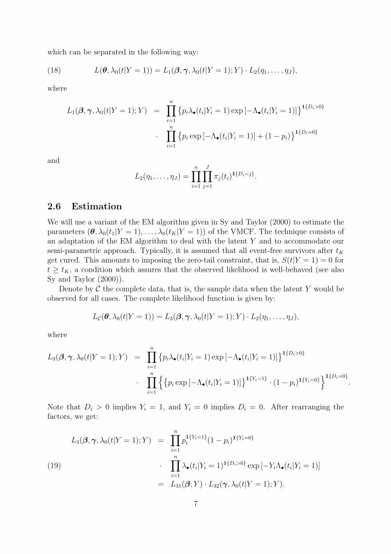
Table 1: Estimated bias (root mean squared error) Fj(t|Y = 1, Z = 1) with respect to thetrue cumulative incidence function Fj(t|Y = 1, Z = 1), j = 1, 2, for the three scenarios.

65% cure in Z = 1 80% cure 20% cure

t F1(t|Y = 1, Z = 1) F2(t|Y = 1, Z = 1) F1(t|Y = 1, Z = 1) F2(t|Y = 1, Z = 1) F1(t|Y = 1, Z = 1) F2(t|Y = 1, Z = 1)

1 -0.0001 (0.0162) -0.0005 (0.0314) -0.0003 (0.0239) -0.0008 (0.0500) -0.0004 (0.0119) -0.0012 (0.0247)2 0.0001 (0.0229) 0.0003 (0.0350) 0.0000 (0.0328) 0.0002 (0.0559) -0.0002 (0.0164) -0.0006 (0.0276)5 0.0012 (0.0302) 0.0036 (0.0337) 0.0018 (0.0419) 0.0057 (0.0495) 0.0004 (0.0208) 0.0015 (0.0240)7 0.0017 (0.0313) 0.0052 (0.0335) 0.0030 (0.0435) 0.0092 (0.0472) 0.0008 (0.0215) 0.0027 (0.0228)10 0.0029 (0.0321) 0.0088 (0.0339) 0.0049 (0.0447) 0.0151 (0.0476) 0.0013 (0.0219) 0.0041 (0.0225)

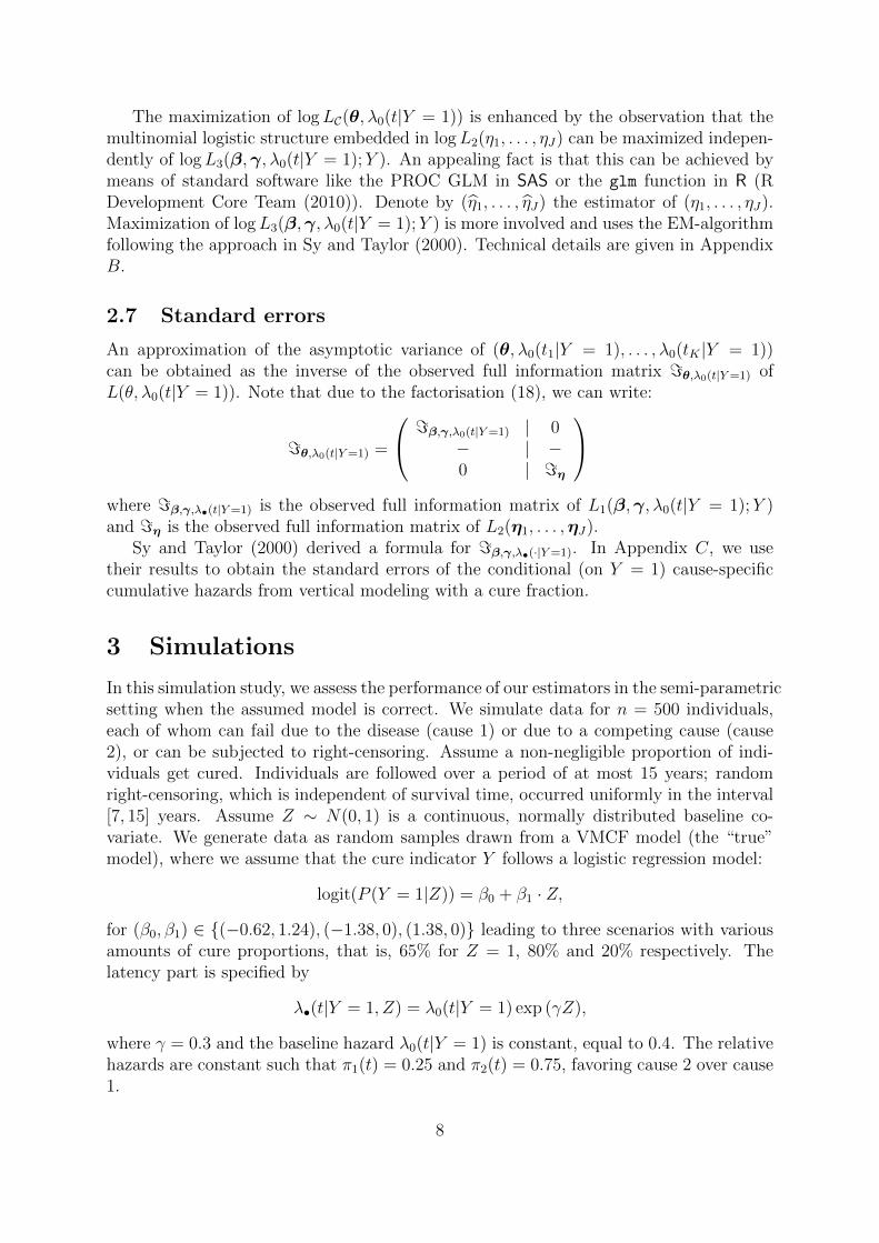
Table 2: Estimated bias (root mean squared error) of Fj(t|Z = 1) with respect to thetrue cumulative incidence function Fj(t|Z = 1), j = 1, 2, in VM and VMCF respectively,when β0 = −0.62, β1 = 1.24 and γ = 0.3.

VM VMCF

t F1(t|Z = 1) F2(t|Z = 1) F1(t|Z = 1) F2(t|Z = 1)

1 -0.0064 (0.0119) -0.0193 (0.0284) 0.0000 (0.0112) 0.0002 (0.0229)2 -0.0086 (0.0170) -0.0260 (0.0366) 0.0004 (0.0160) 0.0012 (0.0281)5 -0.0084 (0.0217) -0.0254 (0.0393) 0.0012 (0.0214) 0.0037 (0.0322)7 -0.0071 (0.0221) -0.0214 (0.0376) 0.0016 (0.0222) 0.0049 (0.0330)10 -0.0053 (0.0222) -0.0159 (0.0353) 0.0024 (0.0228) 0.0073 (0.0338)

The proposed method of estimation VMCF shows little bias in estimating bothFj(t|Y = 1, Z = 1) and Fj(t|Z = 1), with bias (RMSE) increasing with the increasein the cure proportion. The bias contributes little to the RMSE. The behaviour at latertime points is more uncertain due to the smaller number of events by the end of the followup. Comparisons of Fj(t|Z = 1) derived from VMCF and VM with the true cause-specific

9

cumulative incidences consistently show smaller bias (RMSE) for VMCF, thus supportingthe idea that fitting VMCF to data from a population with a non-neglijable proportionof cure can replace a conventional survival model when the interest is to estimate thedisease frequency.

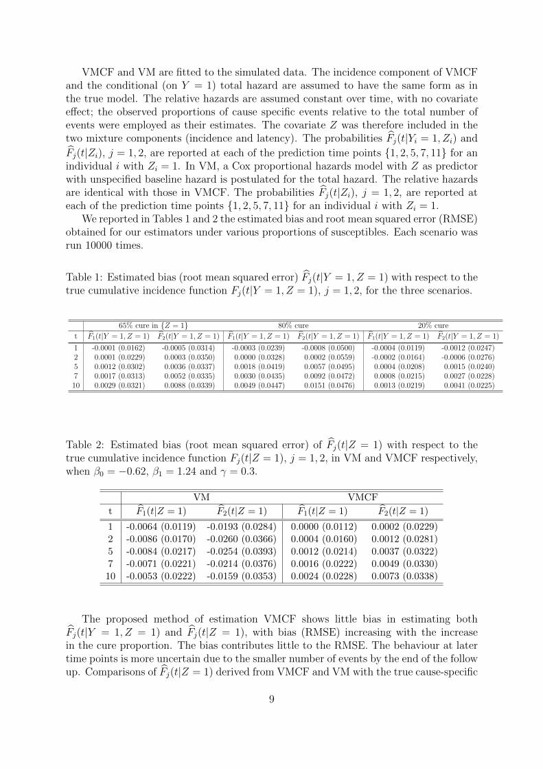
The coverage rates for the normal approximations 95% confidence intervals of Fj(t|Y =

1, Z = 1) and Fj(t|Z = 1) are higher for VMCF compared to VM. They are reported inTable 3 for the first scenario. The other two scenarios, with heavy or small amount ofcure, show the same pattern (not reported).

Table 3: Estimated coverage probabilities of Fj(t|Y = 1, Z = 1) and Fj(t|Z = 1), j = 1, 2in VM and VMCF respectively, when β0 = −0.62, β1 = 1.24 and γ = 0.3.

VMCF VM VMCF

t F1(t|Y = 1, Z = 1) F2(t|Y = 1, Z = 1) F1(t|Z = 1) F2(t|Z = 1) F1(t|Z = 1) F2(t|Z = 1)

1 95.2 95.4 90.8 85.1 95.2 95.52 95.1 95.1 91.6 82.9 95.0 95.05 95.1 95.1 93.3 86.8 95.1 95.27 95.2 95.0 94.2 89.9 95.1 94.810 95.1 94.4 94.8 92.5 95.1 94.6

The performance of estimators β0, β1 and γ was studied in Sy and Taylor (2000).Since these parameters are separated from the parameters of the relative hazards model,the results obtained in Sy and Taylor (2000) are applicable to and were confirmed in oursetting and consequently have not been explored further.

4 Data analysis

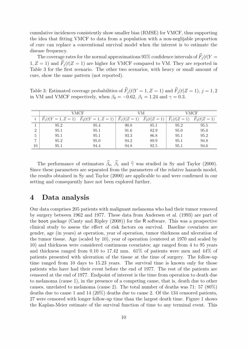
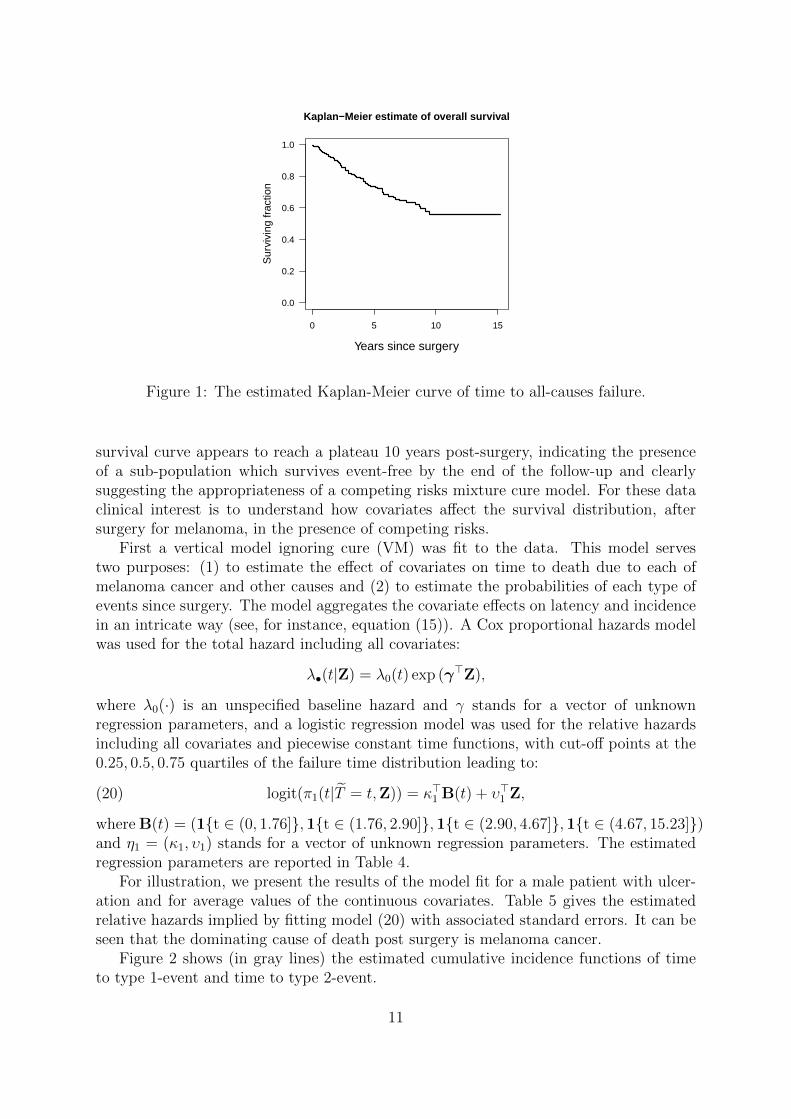
Our data comprises 205 patients with malignant melanoma who had their tumor removedby surgery between 1962 and 1977. These data from Andersen et al. (1993) are part ofthe boot package (Canty and Ripley (2008)) for the R software. This was a prospectiveclinical study to assess the effect of risk factors on survival. Baseline covariates aregender, age (in years) at operation, year of operation, tumor thickness and ulceration ofthe tumor tissue. Age (scaled by 10), year of operation (centered at 1970 and scaled by10) and thickness were considered continuous covariates; age ranged from 4 to 95 yearsand thickness ranged from 0.10 to 17.42 mm. 61% of patients were men and 44% ofpatients presented with ulceration of the tissue at the time of surgery. The follow-uptime ranged from 10 days to 15.23 years. The survival time is known only for thosepatients who have had their event before the end of 1977. The rest of the patients arecensored at the end of 1977. Endpoint of interest is the time from operation to death dueto melanoma (cause 1), in the presence of a competing cause, that is, death due to othercauses, unrelated to melanoma (cause 2). The total number of deaths was 71: 57 (80%)deaths due to cause 1 and 14 (20%) deaths due to cause 2. Of the 134 censored patients,27 were censored with longer follow-up time than the largest death time. Figure 1 showsthe Kaplan-Meier estimate of the survival function of time to any terminal event. This

10

0 5 10 15

0.0

0.2

0.4

0.6

0.8

1.0

Years since surgery

Sur

vivi

ng fr

actio

n

Kaplan−Meier estimate of overall survival

Figure 1: The estimated Kaplan-Meier curve of time to all-causes failure.

survival curve appears to reach a plateau 10 years post-surgery, indicating the presenceof a sub-population which survives event-free by the end of the follow-up and clearlysuggesting the appropriateness of a competing risks mixture cure model. For these dataclinical interest is to understand how covariates affect the survival distribution, aftersurgery for melanoma, in the presence of competing risks.

First a vertical model ignoring cure (VM) was fit to the data. This model servestwo purposes: (1) to estimate the effect of covariates on time to death due to each ofmelanoma cancer and other causes and (2) to estimate the probabilities of each type ofevents since surgery. The model aggregates the covariate effects on latency and incidencein an intricate way (see, for instance, equation (15)). A Cox proportional hazards modelwas used for the total hazard including all covariates:

λ•(t|Z) = λ0(t) exp (γ>Z),

where λ0(·) is an unspecified baseline hazard and γ stands for a vector of unknownregression parameters, and a logistic regression model was used for the relative hazardsincluding all covariates and piecewise constant time functions, with cut-off points at the0.25, 0.5, 0.75 quartiles of the failure time distribution leading to:

(20) logit(π1(t|T = t,Z)) = κ>1 B(t) + υ>1 Z,

where B(t) = (1t ∈ (0, 1.76],1t ∈ (1.76, 2.90],1t ∈ (2.90, 4.67],1t ∈ (4.67, 15.23])and η1 = (κ1, υ1) stands for a vector of unknown regression parameters. The estimatedregression parameters are reported in Table 4.

For illustration, we present the results of the model fit for a male patient with ulcer-ation and for average values of the continuous covariates. Table 5 gives the estimatedrelative hazards implied by fitting model (20) with associated standard errors. It can beseen that the dominating cause of death post surgery is melanoma cancer.

Figure 2 shows (in gray lines) the estimated cumulative incidence functions of timeto type 1-event and time to type 2-event.

11

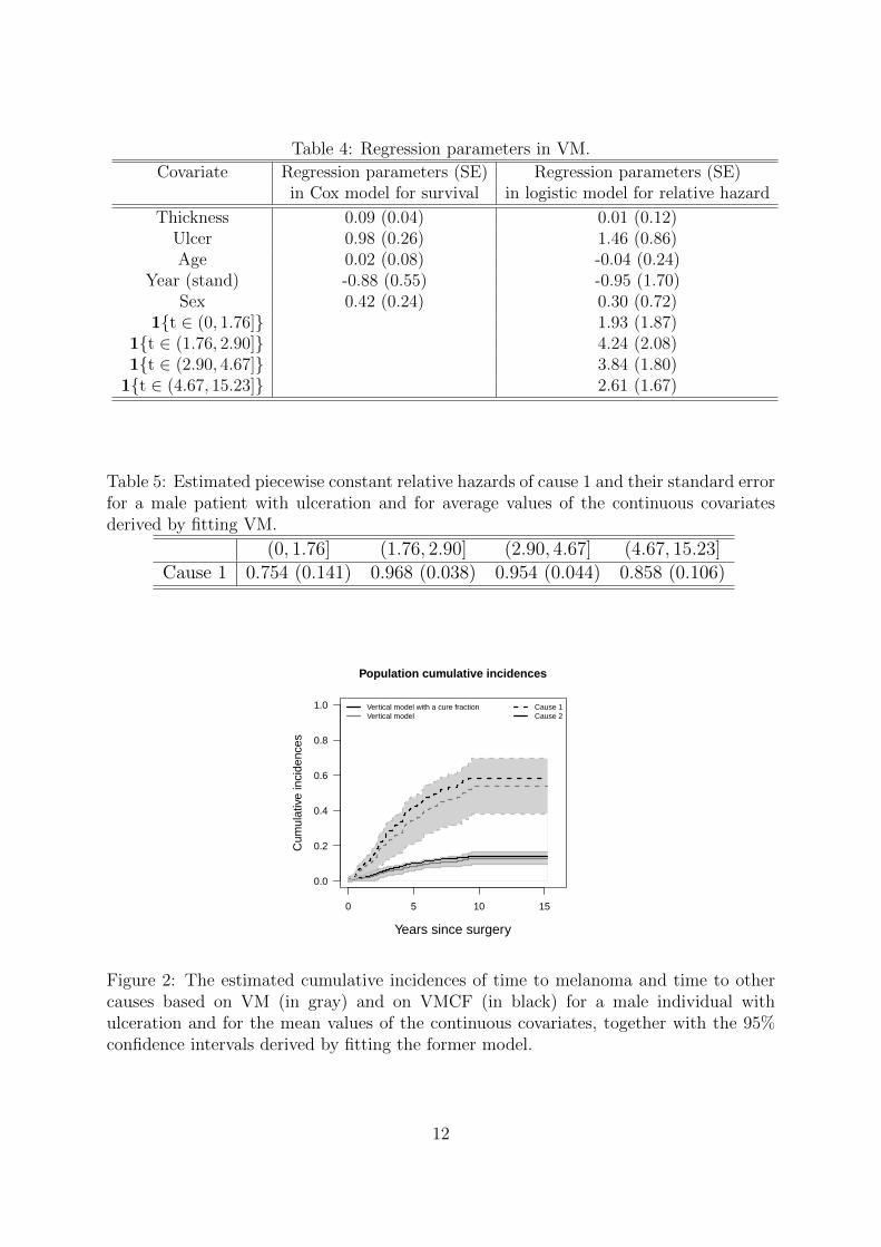
Table 4: Regression parameters in VM.

Covariate Regression parameters (SE) Regression parameters (SE)in Cox model for survival in logistic model for relative hazard

Thickness 0.09 (0.04) 0.01 (0.12)Ulcer 0.98 (0.26) 1.46 (0.86)Age 0.02 (0.08) -0.04 (0.24)

Year (stand) -0.88 (0.55) -0.95 (1.70)Sex 0.42 (0.24) 0.30 (0.72)

1t ∈ (0, 1.76] 1.93 (1.87)1t ∈ (1.76, 2.90] 4.24 (2.08)1t ∈ (2.90, 4.67] 3.84 (1.80)

1t ∈ (4.67, 15.23] 2.61 (1.67)

Table 5: Estimated piecewise constant relative hazards of cause 1 and their standard errorfor a male patient with ulceration and for average values of the continuous covariatesderived by fitting VM.

(0, 1.76] (1.76, 2.90] (2.90, 4.67] (4.67, 15.23]Cause 1 0.754 (0.141) 0.968 (0.038) 0.954 (0.044) 0.858 (0.106)

0 5 10 15

0.0

0.2

0.4

0.6

0.8

1.0

Years since surgery

Cum

ulat

ive

inci

denc

es

Cause 1Cause 2

Vertical model with a cure fractionVertical model

Population cumulative incidences

Figure 2: The estimated cumulative incidences of time to melanoma and time to othercauses based on VM (in gray) and on VMCF (in black) for a male individual withulceration and for the mean values of the continuous covariates, together with the 95%confidence intervals derived by fitting the former model.

12

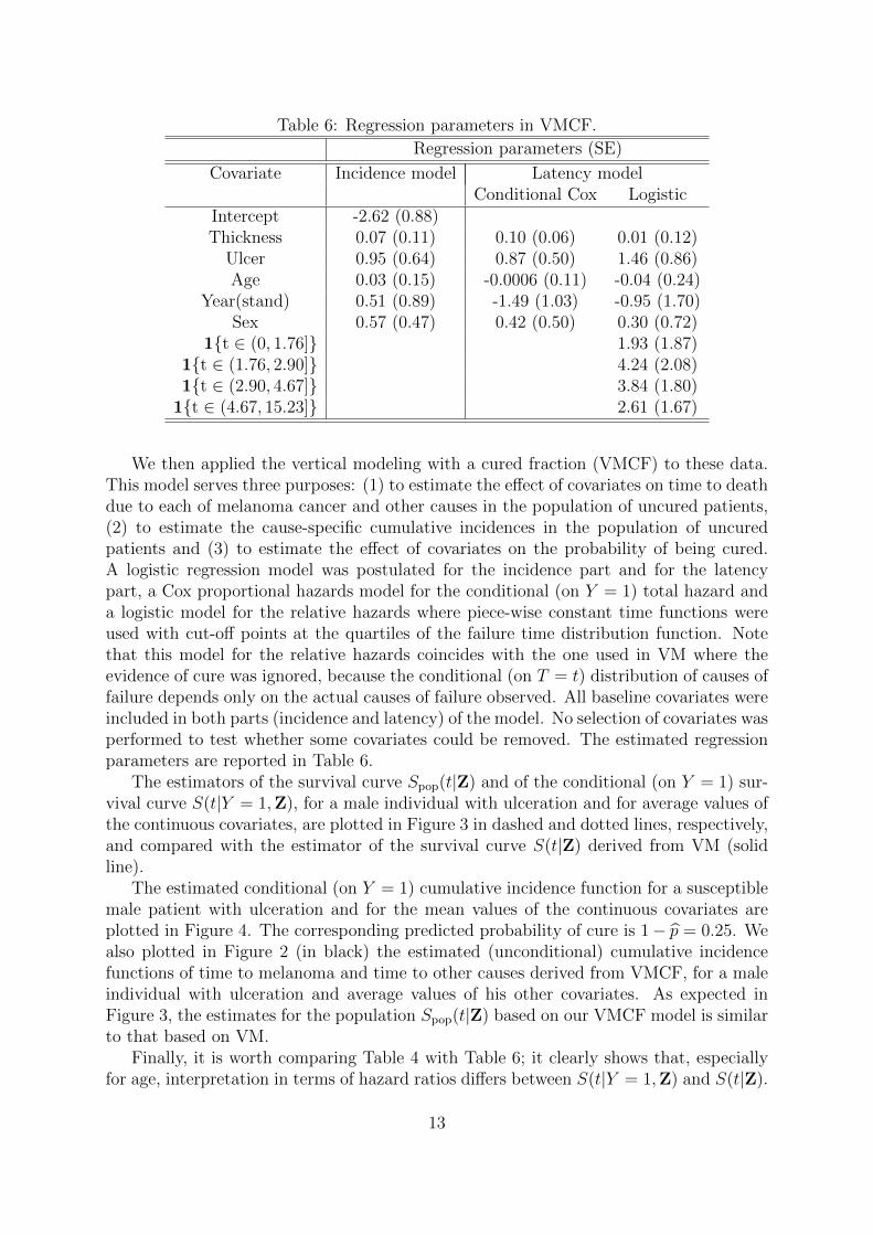
Table 6: Regression parameters in VMCF.

Regression parameters (SE)

Covariate Incidence model Latency modelConditional Cox Logistic

Intercept -2.62 (0.88)Thickness 0.07 (0.11) 0.10 (0.06) 0.01 (0.12)

Ulcer 0.95 (0.64) 0.87 (0.50) 1.46 (0.86)Age 0.03 (0.15) -0.0006 (0.11) -0.04 (0.24)

Year(stand) 0.51 (0.89) -1.49 (1.03) -0.95 (1.70)Sex 0.57 (0.47) 0.42 (0.50) 0.30 (0.72)

1t ∈ (0, 1.76] 1.93 (1.87)1t ∈ (1.76, 2.90] 4.24 (2.08)1t ∈ (2.90, 4.67] 3.84 (1.80)

1t ∈ (4.67, 15.23] 2.61 (1.67)

We then applied the vertical modeling with a cured fraction (VMCF) to these data.This model serves three purposes: (1) to estimate the effect of covariates on time to deathdue to each of melanoma cancer and other causes in the population of uncured patients,(2) to estimate the cause-specific cumulative incidences in the population of uncuredpatients and (3) to estimate the effect of covariates on the probability of being cured.A logistic regression model was postulated for the incidence part and for the latencypart, a Cox proportional hazards model for the conditional (on Y = 1) total hazard anda logistic model for the relative hazards where piece-wise constant time functions wereused with cut-off points at the quartiles of the failure time distribution function. Notethat this model for the relative hazards coincides with the one used in VM where theevidence of cure was ignored, because the conditional (on T = t) distribution of causes offailure depends only on the actual causes of failure observed. All baseline covariates wereincluded in both parts (incidence and latency) of the model. No selection of covariates wasperformed to test whether some covariates could be removed. The estimated regressionparameters are reported in Table 6.

The estimators of the survival curve Spop(t|Z) and of the conditional (on Y = 1) sur-vival curve S(t|Y = 1,Z), for a male individual with ulceration and for average values ofthe continuous covariates, are plotted in Figure 3 in dashed and dotted lines, respectively,and compared with the estimator of the survival curve S(t|Z) derived from VM (solidline).

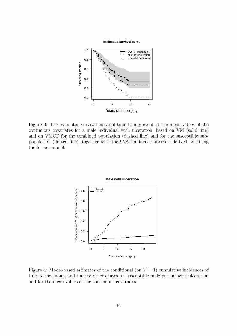
The estimated conditional (on Y = 1) cumulative incidence function for a susceptiblemale patient with ulceration and for the mean values of the continuous covariates areplotted in Figure 4. The corresponding predicted probability of cure is 1− p = 0.25. Wealso plotted in Figure 2 (in black) the estimated (unconditional) cumulative incidencefunctions of time to melanoma and time to other causes derived from VMCF, for a maleindividual with ulceration and average values of his other covariates. As expected inFigure 3, the estimates for the population Spop(t|Z) based on our VMCF model is similarto that based on VM.

Finally, it is worth comparing Table 4 with Table 6; it clearly shows that, especiallyfor age, interpretation in terms of hazard ratios differs between S(t|Y = 1,Z) and S(t|Z).

13

0 5 10 15

0.0

0.2

0.4

0.6

0.8

1.0

Years since surgery

Sur

vivi

ng fr

actio

n

Overall populationMixture populationUncured population

Estimated survival curve

Figure 3: The estimated survival curve of time to any event at the mean values of thecontinuous covariates for a male individual with ulceration, based on VM (solid line)and on VMCF for the combined population (dashed line) and for the susceptible sub-population (dotted line), together with the 95% confidence intervals derived by fittingthe former model.

0 2 4 6 8

0.0

0.2

0.4

0.6

0.8

1.0

Years since surgery

Con

ditio

nal (

on Y

=1)

cum

ulat

ive

inci

denc

es

Cause 1Cause 2

Male with ulceration

Figure 4: Model-based estimates of the conditional (on Y = 1) cumulative incidences oftime to melanoma and time to other causes for susceptible male patient with ulcerationand for the mean values of the continuous covariates.

14

5 Discussion

Little has been published about cure models in combination with competing risks. Severalreviews have been recently published to highlight the advantages of cure models over thelimitations of standard methods like Kaplan-Meier, Cox models or parametric modelsfor survival data when statistical cure is a reasonable assumption (Jia et al. (2013); Yuet al. (2013)). In this paper, we have illustrated a strategy for the statistical analysis ofcompeting risks data with a cure fraction. In this way, we have argued that, when thereis clinical evidence of a cured proportion in a cohort, special attention should be given tothe heterogeneity present among individuals.

An important advantage of the competing risks mixture cure model (VMCF) overthe standard competing risks model (VM) is two-fold: (1) it allows inference of thesusceptible sub-population, and therefore a better understanding and interpretation ofthe variability of the data and (2) it allows estimation and direct modeling of the cureindicator. Summary measures like these can be a useful tool to complement the existingstatistical measures. Each covariate in VMCF can contribute with up to three sets ofregression parameters, one parameter reflecting how the covariate affects the chance ofcure, one parameter for the risk of failure, irrespective of the cause of failure, and one setof parameters for the relative position of each failure type among all failure types.

An appealing technical feature of VMCF resides in its parametrisation, which is il-lustrated in equation (18). VMCF naturally separates the observed likelihood into twofactors: one where the cure indicator distribution is irrelevant and one where the cureindicator distribution is relevant. The former factor is pertinent to causes of failure whena failure occurs; in the absence of competing events, the observed likelihood (18) re-duces to the observed likelihood of the Cox proportional hazards mixture cure model ofSy and Taylor (2000). The latter factor uses information on the failure and censoringtimes and, therefore, it is sensitive to the joint distribution of (T, Y ). This feature makesour method straighforward to implement by means of smcure package available in RDevelopment Core Team (2010).

We believe that our approach can play a useful role, as it can accommodate complexcompeting risks data. It is worth mentioning that the approach can be naturally extendedto deal with missing causes of failure in competing risks. We refer to the work of Nicolaieet al. (2011) for a description of how this can be achieved.

An important issue is that semi-parametric mixture cure models are by constructionnon-identifiable. We cannot precisely tell apart individuals who are cured or not amongthose who are censored. However, the presence of individuals with long follow-up andevent-free works as empirical evidence of the existence of a cured subgroup. We adopt thestrategy of Sy and Taylor (2000), who approach the non-identifiability problem throughthe use of the zero-tail constraint on the baseline failure time distribution. Anotherstrategy has been adopted by Peng (2003), who impose a parametric shape on the tail ofthe failure time distribution.

Another aspect goes to the core of how cure is perceived in the presence of competingrisks, other than the risk that is related to the disease. It might be the case that a diseasedpatient is at risk of several mutually exclusive causes of failure and their potential curefrom the disease cannot be observed if they die from accidental causes. For instance, adifferent formulation is proposed by Basu and Tiwari (2010), where separate competing

15

risks structures are considered for the cure and the susceptible latent groups and a jointprior distribution is assumed on the collection of parameters. Cure is defined as nothaving experienced death due to the disease-related cause; therefore, the status of cureis observed only for individuals subjected to death not due to the cause of interest. Weare currently adapting the vertical modeling approach to this situation.

Acknowledgements

Research supported by IAP research network grant nr. P7/06 of the Belgian government(Belgian Science Policy). C. Legrand is supported by the contract ’Projet d’Actionsde Recherche Concertees’ (ARC) 11/16-039 of the ’Communaute francaise de Belgique’,granted by the ’Academie universitaire Louvain’.

References

Andersen, P. K., O. Borgan, R. D. Gill, and N. Keiding (1993). Statistical Models basedon Counting Processes. Springer.

Andersson, T. M. L., P. W. Dickman, S. Eloranta, and P. C. Lambert (2011). Estimatingand modelling cure in population-based cancer studies within the framework of flexibleparametric survival models. BMC Medical Research Methodology 11, 1–11.

Andrae, B., T. M. L. Andersson, P. C. Lambert, L. Kemetli, L. Silverdal, B. Strander,W. Ryd, J. Dillner, S. Tolnber, and P. Sparen (2012). Screening and cervical cancercure: population based cohort study. British Medical Journal 344, e900.

Basu, S. and T. C. Tiwari (2010). Breast cancer survival, competing risks and mixturecure model: a Bayesian analysis. Journal of the Royal Statistical Society: Series A 173,307–329.

Canty, A. and B. Ripley (2008). boot: Bootstrap r (s-plus) functions. R package version1.2-34.

Chao, E. C. (1998). Gibbs sampling for long-term survival data with competing risks.Communication in Statistics: Theory and Methods 54, 350–366.

Choi, K. C. and X. Zhou (2002). Large sample properties of mixture models with covari-ates competing risks. Journal of Multivariate Analysis 82, 331–366.

Corbiere, F., D. Commenges, J. M. G. Taylor, and P. Joly (2009). A penalized likelihoodapproach for mixture cure models. Statistics in Medicine 28, 510–524.

Farewell, V. T. (1986). Mixture models in survival analysis: are they worth the risk?The Canadian Journal of Statistics 14, 257–262.

Jia, X., C. S. Sima, M. F. Brennan, and K. S. Panageas (2013). Cure models for theanalysis of time-to-event data in cancer studies. Journal of Surgical Oncology 108,342–347.

16

Kim, S., D. Zeng, Y. Li, and D. Spiegelman (2013). Joint modeling of longitudinal andcure survival data. Journal of Statistical Theory and Practice 7, 324–344.

Kuk, A. Y. C. and C. Chen (1992). A mixture model combining logistic regression withproportional hazards regression. Biometrika 79, 531–541.

Larson, M. G. and G. E. Dinse (1985). A mixture model for the regression analysis ofcompeting risks data. Applied Statistics 34, 201–211.

Li, C.-S. and J. M. G. Taylor (2002). A semiparametric accelerated failure time curemodel. Statistics in Medicine 21, 3235–3247.

Ng, S. K. and G. J. McLachlan (1998). On modifications to the long-term survivalmixture model in the presence of competing risks. Journal of Statistical Computationand Simulation 61, 77–96.

Nicolaie, M. A., H. Putter, and J. C. van Houwelingen (2010). Vertical modeling: apattern mixture approach for competing risks data. Statistics in Medicine 29, 1190–1205.

Nicolaie, M. A., H. Putter, and J. C. van Houwelingen (2011). Vertical modeling: analysisof competing risks data with missing causes of failure. Statistical Methods in MedicalResearch In print, DOI:10.1177/0962280211432067.

Peng, Y. (2003). Estimating baseline distribution in proportional hazards cure models.Computational Statistics and Data Analysis 42, 187–201.

Peng, Y. and K. B. G. Dear (2000). A nonparametric mixture model for cure rateestimation. Biometrics 56, 2236–243.

R Development Core Team (2010). R: A language and environment for statistical com-puting. R Foundation for Statistical Computing Vienna, Austria.

Sy, J. P. and J. M. G. Taylor (2000). Estimation in a Cox proportional hazards curemodel. Biometrics 56, 227–236.

Taylor, J. M. G. (1995). Semi-parametric estimation in failure time mixture models.Biometrics 51, 899–907.

Yu, M., N. J. Law, J. M. G. Taylor, and H. M. Sandler (2004). Joint longitudinal survival-cure models and their application to prostate cancer. Statistica Sinica 14, 835–862.

Yu, X. Q., R. De Angelis, T. M. L. Andersson, P. C. Lambert, and P. Dickman (2013).Estimating the proportion cured of cancer: some practical advice for users. CancerEpidemiology 37, 836–842.

17

Appendix A: Derivation of formula (17)

Using (16), the hazard ratio corresponding to two individuals with covariate values given

by Z and Z is given byλ•,pop(t|Z)

λ•,pop(t|Z)= eη

>(t)(Z−Z).

On the other hand, using (15), the same hazard ratio is given by

λ•,pop(t|Z,X)

λ•,pop(t|Z, X)= eγ

>(Z−Z) · E[Y |T ≥ t,Z,X]

E[Y |T ≥ t, Z, X],

Equating the two representations leads to

η>(t)(Z− Z) = γ>(Z− Z) + logE[Y |T ≥ t,Z,X]

E[Y |T ≥ t, Z, X]

whose k-th component is given by (17).

Appendix B: The EM-algorithm

In the E-step of the algorithm the conditional expectation of logL3(β,γ, λ0(t|Y = 1);Y )is computed with respect to the distribution of the unobserved Yi’s, given the currentparameters values and the observed data O = (Oi)i=1,...,n. As Yi’s contribute as linearterms in logL3(β,γ, λ0(t|Y = 1);Y ), it is enough to compute, at a given iteration m,

the weight w(m)i = E(Yi|θ(m), λ

(m)0 (t|Y = 1),O). For an individual i who experiences an

event at time ti (irrespective of its cause) the corresponding weight is

w(m)i = E(Y |θ(m), λ

(m)0 (ti|Y = 1), T = ti, Di ∈ 1, . . . , J)

= P (Yi = 1|θ(m), λ(m)0 (ti|Y = 1), T = ti, Di ∈ 1, . . . , J)

= 1,

while for an individual i who is censored at time ti the corresponding weight is

w(m)i = E(Y |θ(m), λ

(m)0 (ti|Y = 1), T > ti, Di = 0)

= P (Yi = 1|θ(m), λ(m)0 (ti|Y = 1), T > ti, Di = 0)

=g−1(β>X∗i ) · S0(ti|Y = 1)exp(γ>Zi)

g−1(β>X∗i ) · S0(ti|Y = 1)exp(γ>Zi) + 1− g−1(β>X∗i )

∣∣∣∣∣(θ,λ0(ti|Y=1))=(θ(m),λ

(m)0 (ti|Y=1))

.

Denote the expected complete log-likelihood by Ep[logL3(β,γ, λ0(ti|Y = 1);w(m))|O],

where w(m) = (w(m)i )i=1,...,n.

In the M -step of the algorithm, Ep[logL3(β,γ, λ0(t|Y = 1);w(m))|O] is maximizedwith respect to (β,γ, λ0(t|Y = 1), given w(m). Unlike in the standard Cox proportionalhazards model, where the baseline hazard is seen as a nuisance parameter and eliminatedin the procedure of estimating γ, one cannot eliminate λ0(t|Y = 1) in the Cox propor-tional hazards model embedded in the VMCF without loosing information about β. The

18

main reason is that the hazard rate at the population level is no longer proportional(see (15) and (16)) and arguments similar to those leading to the Cox partial likelihooddo not hold true anymore. Peng and Dear (2000), Sy and Taylor (2000) proposed apartial likelihood type method to estimate γ without specifying the nuisance parameterΛ0(t|Y = 1). This involves the updating of the Aalen-Nelson estimator of Λ0(t|Y = 1) atthe mth iteration as given by

Λ0(t|Y = 1) =∑i:ti≤t

di∑l∈Ri

w(m)l exp(γ>Zl)

,

where di is the number of events at time ti, irrespective of the cause, and Ri is the risk setat ti. By substituting Λ0(t|Y = 1) into logL32(γ, λ0(t|Y = 1);w(m)) we get the weightedpartial likelihood of γ, that is

n∏i=1

[ exp(γ>Zi)∑l∈Ri

w(m)l exp(γ>Zl)

]1Di>0.

To assure identifiability, we impose the zero-tail constraint (see Sy and Taylor (2000)),

that is, S0(t|Y = 1) = 0 for t > tK .

Appendix C: The standard errors of conditional (on

Y = 1) cumulative hazards from vertical modeling with

a cure fraction

In this appendix we derive the formula for the standard error of the conditional (on Y = 1)cause-specific cumulative hazard from vertical modeling with a cure fraction, when weomit the vector Z of covariates from the model of the latency component. As a conse-quence, the vector of parameter describing VMCF is (β,η, λ•(t1|Y = 1), . . . , λ•(tK |Y =1)).

The Nelson-Aalen estimator of Λ•(t|Y = 1), denoted by Λ•(t|Y = 1), makes jumps

of size dΛ•(t|Y = 1) at event time points 0 = t0 ≤ t1 < t2 < . . . < tK < ∞. An

approximation of the covariance matrix of (β, dΛ•(t1|Y = 1), . . . , dΛ•(tK |Y = 1)) isgiven by the inverse of the observed full information matrix =β,dΛ•(·|Y=1).

Remark. The matrix =β,dΛ•(·|Y=1) is not diagonal. Let Ξβ,dΛ•(·|Y=1) denote an inverseof =β,dΛ•(·|Y=1) and let ΞdΛ•(·|Y=1) be the sub-matrix of Ξβ,dΛ•(·|Y=1) corresponding to

dΛ•(·|Y = 1).Relevant quantities for our purposes are the relative hazards πj(t); we model them as

in formula (12).Remark. Often it will convenient to retain the system (12) and to work with the r×J

Fisher information matrix of η> =(η1, . . . , ηJ

)>, denoted by =η which has rank r(J − 1)

and, in particular, is not invertible. Let Ξη denote a Moore-Penrose generalized inverseof =η.

We are interested to develop a formula for the JK×JK covariance matrix var(Λ(·|Y =

1)) =: ΞΛ of the estimator Λj(t|Y = 1) =∑

ts≤t πj(ts)λ•(ts|Y = 1) =∑

ts≤t λjs,Y=1,

19

where λjs,Y=1 = πj(ts)λ•(ts|Y = 1). First, we introduce some notation, as follows:

τ = (η, λ•(t1|Y = 1), . . . , λ•(tK |Y = 1))> ,

Λ =((Λj(t1|Y = 1))j=1,...,J , (Λj(t2|Y = 1))j=1,...,J , . . . , (Λj(tK |Y = 1))j=1,...,J

)>and

λ =(λ11,Y=1, λ21,Y=1, . . . , λJ1,Y=1, λ12,Y=1, . . . , λJ2,Y=1, λ1K,Y=1, . . . , λJK,Y=1

).

According to the Delta-method, we get

(21) ΞΛ =∂Λ(·|Y = 1)

∂λ(·|Y = 1)· ∂λ(·|Y = 1)

∂τ· var(τ ) ·

(∂Λ(·|Y = 1)

∂λ(·|Y = 1)· ∂λ(·|Y = 1)

∂τ

)>.

It is straightforward to see that the matrix ∂Λ∂λ

of order JK is given by

(22)∂Λ

∂λ=

IJ×J 0 0 0IJ×J IJ×J 0 0

. . . . . .. . . . . .

. . . 0IJ×J IJ×J . . . IJ×J

where IJ×J is the identity matrix of order J . Also, we have

∂λjs,Y=1

∂ηlu= −πj(ts)πl(ts)λ•(ts|Y = 1)Bu(ts) ,

where j, l ∈ 1, . . . , J, j 6= l, s ∈ 1, . . . , K, u ∈ 1, . . . , r, and

∂λjs,Y=1

∂ηju= πj(ts)

[1− πj(ts)

]λ•(ts|Y = 1)Bu(ts) ,

where j ∈ 1, . . . , J, s ∈ 1, . . . , K, u ∈ 1, . . . , r.Moreover,

∂λjs,Y=1

∂λ•(tv|Y = 1)= πj(ts)δs,v ,

where j ∈ 1, . . . , J, s, v ∈ 1, . . . , K and δ stands for the Kronecker delta.We shall define, for t ≥ 0, the J × J matrix Ω(t) as follows:

Ω(t) =

π1(t) 0 . . . 0

0 π2(t) . . . 0. . . . . . . . . . . .0 0 . . . πJ(t)

− (π1(t), π2(t), . . . , πJ(t))>(

π1(t), π2(t), . . . , πJ(t)),

and the r-vector

α(t) =(λ•(t|Y = 1)B1(t), λ•(t|Y = 1)B2(t), . . . , λ•(t|Y = 1)Br(t)

)>.

20

Setting

Π(ts) =(π1(ts), π2(ts), . . . , πJ(ts)

)>,

a column vector of length J , for s ∈ 1, . . . , K, we get

(23)∂(λ1s,Y=1, λ2s,Y=1, . . . , λJs,Y=1)

∂(η1, η2, . . . , ηJ)= Ω(ts)⊗ (α(ts))

>, s ∈ 1, . . . , K ,

where ⊗ stands for the Kronecker product, and finally

(24)∂λ

∂τ=

Ω(t1)⊗ (α(t1))> Π(t1) 0 0 0Ω(t2)⊗ (α(t2))> 0 Π(t2) 0 0

0. . . . . .

......

. . . . . . . . .. . . . . . 0

Ω(tK)⊗ (α(tK))> 0 0 0 . . . 0 Π(tK)

which is a matrix of order JK × (Jr +K). As a result, we obtain

(25) Ξλ =∂λ

∂τ

Ξη | 0− | −0 | ΞdΛ•(·|Y=1)

(∂λ∂τ

)>.

In conclusion, using (21), (22) and (25), we have that

(26) ΞΛ =

W1ΞηW1 + Π1 W1ΞηW2 + Π1 . . . W1ΞηWK + Π1

W2ΞηW1 + Π1 W2ΞηW2 + Π2 . . . W2ΞηWK + Π2...

.... . .

...

WKΞηW1 + Π1 WKΞηW2 + Π2 . . . WKΞηWK + ΠK

,

where

Wk =k∑s=1

Ω(ts)⊗ (α(ts))>, k ∈ 1, . . . , K ,

and

Πkl =k∑l=1

ΞdΛ•(·|Y=1) ⊗( k∑s=1

Π(ts)(Π(tl))>), k, l ∈ 1, . . . , K .

21