DPRIETI Discussion Paper Series 03-E-001

Vertical Intra-Industry Trade and Foreign Direct Investmentin East Asia

ISHIDO HikariInstitute of Developing Economies

ITO KeikoInternational Centre for the Study of East Asian Development

FUKAO KyojiRIETI

The Research Institute of Economy, Trade and Industryhttp://www.rieti.go.jp/en/

RIETI Discussion Paper Series 03-E-001

Vertical Intra-Industry Trade and Foreign Direct Investment in East Asia

Kyoji Fukao*

Hitotsubashi University, ADBI and RIETI

Hikari Ishido

Institute of Developing Economies

Keiko Ito

International Centre for the Study of East Asian Development

Revised Version, January 2003

* Correspondence: Kyoji Fukao, Institute of Economic Research, Hitotsubashi University, Naka 2-1, Kunitachi, Tokyo 186-8603 JAPAN. Tel.: +81-42-580-8359, Fax.: +81-42-580 -8333, e-mail: k.fukao@srv.cc.hit-u.ac.jp We would like to thank ADBI for its financial support. The authors are grateful to Yoshimasa Yoshiike for undertaking meticulous data calculations. The previous version of this paper was presented at the 15th Annual TRIO Conference Supported by NBER-CEPR-TCER-RIETI, New Development in Empirical International Trade, December 10-11, 2002, International House of Japan, Tokyo. The authors are grateful for the comments by James Harrigan, Shujiro Urata, and other conference participants.

1

Abstract

As economic integration in East Asia progresses, trade patterns within the region are displaying an ever-greater complexity: Though inter-industry trade still accounts for the majority, its share in overall trade is declining. Instead, intra-industry trade (IIT), which can be further divided into horizontal IIT (HIIT) and vertical IIT (VIIT), is growing in importance.

In this paper, we set out to measure and examine vertical intra-industry trade patterns in the East Asian region and compare these with the results of previous studies focusing on the EU, to which such analyses so far have been confined. Based on the supposition that VIIT is closely related to offshore production by multinational enterprises, we then develop a model to capture the main determinants of VIIT that explicitly includes the role of FDI. The model is tested empirically using data from the electrical machinery industry. The findings support our hypothesis, showing that FDI plays a significant role in the rapid increase in VIIT in East Asia seen in recent years.

JEL Classification: F14, F23 Key Words: Vertical Intra-Industry Trade, Vertical Foreign Direct Investment, East Asia, European Union

2

1. Introduction

Recent studies on intra-industry trade (IIT) have brought to light rapid increases in

vertical IIT, i.e. intra-industry trade where goods are differentiated by quality.1 As Falvey

(1981) pointed out in his seminal theoretical paper, commodities of the same statistical group

but of different quality may be produced using different mixes of factor inputs. Moreover,

developed economies may export physical and human capital-intensive products of

high-quality and import unskilled labor-intensive products of low-quality from developing

economies. Through this mechanism, an increase in vertical IIT may have a large impact on

factor demands and factor prices in Japan and elsewhere.2

Vertical IIT is likely to be driven by differences in factor endowments. Consequently,

we expect vertical IIT to be more pronounced between developing and developed economies.

At the same time, however, developing economies rarely possess the technology to produce

commodities that belong to the same statistical categories as the commodities exported by the

developed economies, such as telecommunications equipment and advanced office

machinery.

Developing economies’ main source of advanced technology in recent years probably

has been inward direct investment. A major part of vertical IIT may be conducted by

multinational enterprises in the context of the international division of labor. In East Asia,

efficiency-seeking and export-oriented foreign direct investments (FDI) mainly from Japan

and the United States have increased rapidly over the last decade. As a result, we would

expect active vertical IIT between developing economies in East Asia and Japan and the

United States.

Despite the potential importance of this issue and the fact that theory suggests that the

determinants of vertical and horizontal IIT differ, most of previous empirical studies on IIT in

East Asia have focused on total IIT without distinguishing between vertical and horizontal

1 Several studies on vertical IIT have been conducted for European countries and the United States. Based on trade statistics for the United Kingdom, Greenaway, Hine and Milner (1994), and Greenaway, Hine, and Milner (1995) studied how country- or industry-specific factors affect the relative importance of vertical and horizontal IIT. Aturupane, Djankov and Hoekman (1999) studied the same type of issues in the case of IIT between Eastern Europe and the European Union. Differentiating between vertical and horizontal IIT, Fontagné, Freudenberg, and Péridy (1997) carried out a detailed investigation of trade patterns within the European Union. 2 The “fragmentation” of production processes, that is, the international division of labor in production processes and the increase in the trade in intermediate inputs of different factor contents, may have the same kind of impact. Feenstra and Hanson (2001) provide a survey of studies on this issue. Several studies have found that multinational enterprises play a key role in the “fragmentation” (see Feenstra and Hanson 1996, Slaughter 2000, Head and Ries 2000, Kimura and Fukasaku 2001, and Kimura 2001). Since there already exist many theoretical and empirical studies on this issue, we do not focus on “fragmentation” in this paper.

3

IIT.3 In this paper, we review vertical and horizontal IIT in East Asia and compare it with

trade patterns in other regions, particularly the European Union. We will also construct a

theoretical model to understand the relationship between vertical IIT and FDI. Based on the

model we will conduct an econometric analysis in order to determine what country specific

factors determine the size of vertical IIT. For the econometric analysis we will use statistics

of Japan’s electrical machinery trade at the HS (Harmonized Commodity Description and

Coding System) 9-digit level.

The remainder of the paper is organized as follows. In Section 2 we provide an

overview of trade and FDI patterns in East Asia and present a descriptive analysis. In

Section 3 we review existing theories of IIT and propose a theoretical model which explains

the relationship between FDI and vertical IIT. In section 4 we conduct an econometric

analysis of the determinants of vertical IIT. Section 5 summarizes the main findings of this

paper.

2. Descriptive Analysis

2.1. Major Characteristics of Economic Development and Integration in East Asia

As a first step of our descriptive analysis we present an overview of the trade patterns of

the East Asian economies.

In the last two decades, the countries of East Asia accomplished rapid economic growth

based on trade expansion. Table 2-1 shows the export-GDP and import-GDP ratios of East

Asia and other regions. In the 1980s and 90s, the dependence on international trade

increased at an amazing speed in the case of the ASEAN-4, China and Hong Kong.

Compared with this, the ratio has not increased substantially for the EU or MERCOSUR.

The East Asian countries increased not only their exports of labor-intensive products, such as

apparels and leather products, but also of technology-intensive products, such as electrical

machinery and telecommunications equipment. Economic development of the

“leapfrogging” type has occurred in the East Asian countries. A good example for this is

China, which is competitive not only in the export of labor-intensive but also of high-tech

products such as office machines and telecommunication apparatuses. The share of China’s

exports in world total imports is rapidly catching up with Japan’s in many high-tech product

categories. The share of China’s and Hong Kong’s combined exports in world total imports

3 Abe (1997) and Murshed (2001) studied IIT of the East Asian countries without distinguishing between vertical and horizontal IIT. Based on Japan’s trade statistics at the HS 9-digit level, Yoshiike (2002) and Ishida (2002) found that Japan has substantially increased its vertical IIT with the East Asian countries during the last decade. Using relatively aggregated trade data (SITC 3-digit level), Hu and Ma (1999) have studied the vertical IIT of China.

4

in 1999 was 9.3% in the case of telecommunications and sound recording apparatus (SITC R3

#76) and 6.5% in the case of office machines and automatic data processing machines (SITC

R3 #75), whereas Japan’s shares in these categories were 11.2% and 9.7% respectively. 4

INSERT TABLE 2-1

In the case of technology-intensive products, we also observe very active IIT among the

East Asian countries. In 1999, Japan exported 272.4 billion yen worth of

telecommunications equipment and parts (SITC R3 #764) to China and Hong Kong and

imported 221.8 billion yen worth of the same products from these two economies. Similarly,

in the case of television receivers (SITC R3 #761), Japan exported to and imported from

China and Hong Kong 37.5 billion yen and 39.5 billion yen worth of merchandise

respectively in 1999.

The East Asian countries’ export-led growth has depended not only on regional trade,

but also on trade with other regions. Table 2-2 shows the trade matrix of IT-related products

for trade among Japan, Asia (excluding Japan), the US and the EU. Compared with the EU

countries, which depend more on the regional market, the Asian countries depend on the US

and the EU markets.5 The reason for this is that East Asia is a major supplier of IT products

for the world market, not only for the regional market.

INSERT TABLES 2-2 and 2-3

A very important role in East Asian development was also played by inward FDI.

Table 2-3 shows the inward FDI stock as a percentage of GDP by region. In the case of the

East and Southeast Asian countries, excluding Japan, the inward FDI/GDP ratio is very high

compared with the EU, North America, or Latin America. It seems that this is the most

important characteristic, and that the other characteristics such as export-led growth and

leapfrogging-type development pointed out above have mainly been created by active inward

FDI. For example, FDI in this region is very export-oriented. Table 2-4 compares the sales

destinations of foreign manufacturing affiliates of Japanese and US firms by host region.

This table shows that affiliates in East Asia owned by Japanese and US firms are more export

oriented than affiliates in other regions. Japanese and US direct investments in East Asia

seem to be “vertical” in the sense that manufacturing affiliates are established in order to take

4 These data are taken from Statistics Canada, World Trade Analyzer 1980-99. 5 For details on this issue, see Urata (2002).

5

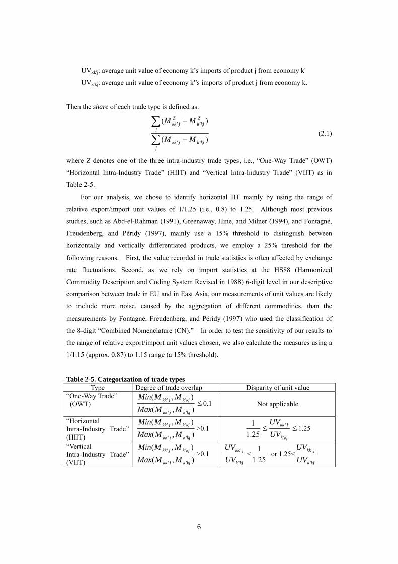
advantage of cheap labor, and the majority of the output is exported to their home countries or

other countries. According to the standard theory of FDI, multinational enterprises tend to

conduct FDI of the “vertical type” when there is a huge gap in factor prices between their

home and the host country, and when the market of the host county is relatively small and

trade costs are not large.6 Developing economies in East Asia seem to satisfy these

conditions and attract “vertical” FDI.7

Export-led growth and leapfrogging development is caused by FDI. We can confirm

this if we look at the statistics on the production share of affiliates owned by foreign firms in

China. In industries which experienced export-led growth, for example garments, leather,

and electric and telecommunications equipment, the share of foreign affiliates in value-added

is close to or greater than 50%.8 Thus, it is fair to say that China’s amazing export-led

growth in fact has been brought about by foreign firms.

INSERT TABLE 2-4

2.2. Measurement of Intra-Industry Trade: Threshold-Based Indices

In order to identify vertical and horizontal IIT we adopt a methodology used by major

preceding studies on vertical IIT, such as Greenaway, Hine, and Milner (1995), Fontagné,

Freudenberg, and Péridy (1997), and Aturupane, Djankov, and Hoekman (1999). The

methodology is based on the assumption that the gap between the unit value of imports and

the unit value of exports for each commodity reveals the qualitative differences of the

products exported and imported between the two economies.

We break down the bilateral trade flows of each detailed commodity category into the

three patterns: (a) inter-industry trade (one-way trade), (b) intra-industry trade (IIT) in

horizontally differentiated products (products differentiated by attributes), and (c) IIT in

vertically differentiated products (products differentiated by quality).

M kk'j: value of economy k’s imports of product j from economy k'

Mk'kj: value of economy k'’s imports of product j from economy k 6 For more details on this issue, see Markusen (1995), Markusen, Venables, Konan and Zhang (1996), and Carr, Markusen and Maskus (2001). 7 For East Asian manufacturing affiliates owned by foreign firms, trade costs depend on their location and the category of commodities they import and export. These affiliates are located mainly in coastal areas and the infrastructure of East Asian ports is relatively efficient. Additionally, export oriented affiliates can usually get special tariff-reductions for their imports of intermediate inputs. Because of these factors, the affiliates seem to face relatively small trade costs. 8 For more details, see China Statistical Yearbook 2001, National Bureau of Statistics of China, China Statistics Press, Beijing, China 2001. We should note that in China’s statistics affiliates owned by Hong Kong and Taiwanese firms are included under foreign-owned affiliates.

6

UVkk'j: average unit value of economy k’s imports of product j from economy k'

UVk'kj: average unit value of economy k'’s imports of product j from economy k.

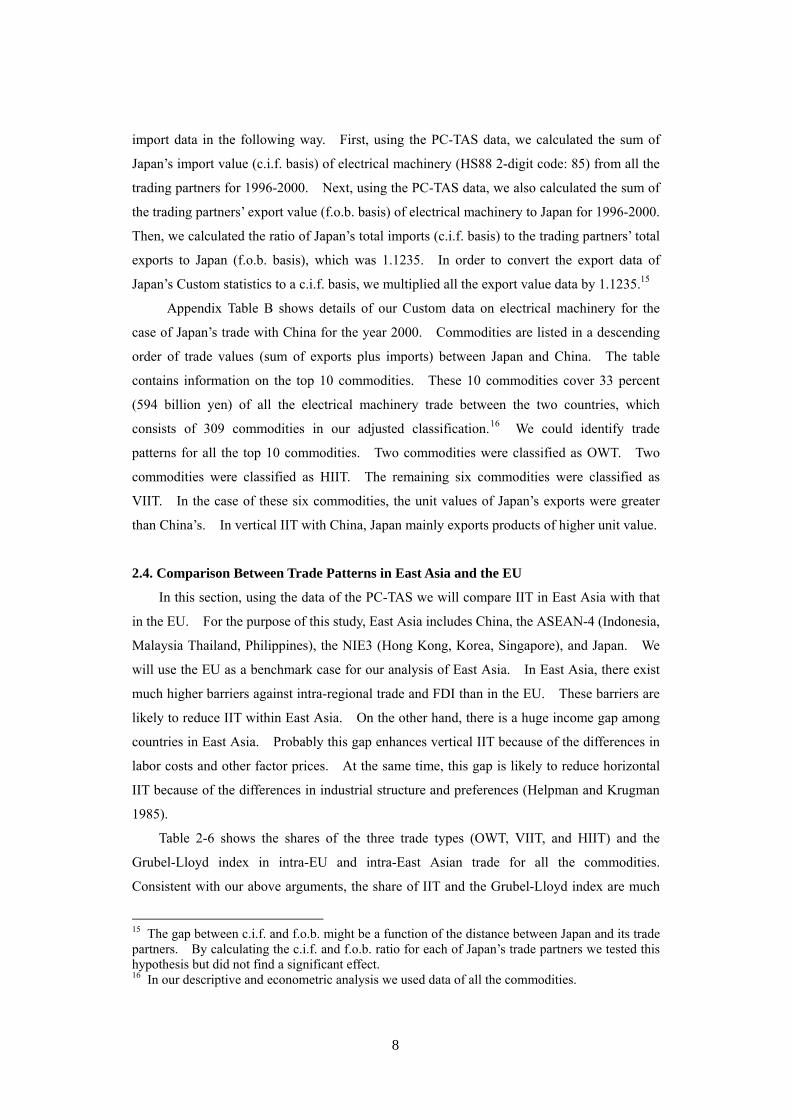
Then the share of each trade type is defined as:

∑∑

+

+

jkjkjkk

j

Zkjk

Zjkk

MM

MM

)(

)(

''

''

(2.1)

where Z denotes one of the three intra-industry trade types, i.e., “One-Way Trade” (OWT)

“Horizontal Intra-Industry Trade” (HIIT) and “Vertical Intra-Industry Trade” (VIIT) as in

Table 2-5.

For our analysis, we chose to identify horizontal IIT mainly by using the range of

relative export/import unit values of 1/1.25 (i.e., 0.8) to 1.25. Although most previous

studies, such as Abd-el-Rahman (1991), Greenaway, Hine, and Milner (1994), and Fontagné,

Freudenberg, and Péridy (1997), mainly use a 15% threshold to distinguish between

horizontally and vertically differentiated products, we employ a 25% threshold for the

following reasons. First, the value recorded in trade statistics is often affected by exchange

rate fluctuations. Second, as we rely on import statistics at the HS88 (Harmonized

Commodity Description and Coding System Revised in 1988) 6-digit level in our descriptive

comparison between trade in EU and in East Asia, our measurements of unit values are likely

to include more noise, caused by the aggregation of different commodities, than the

measurements by Fontagné, Freudenberg, and Péridy (1997) who used the classification of

the 8-digit “Combined Nomenclature (CN).” In order to test the sensitivity of our results to

the range of relative export/import unit values chosen, we also calculate the measures using a

1/1.15 (approx. 0.87) to 1.15 range (a 15% threshold).

Table 2-5. Categorization of trade types Type Degree of trade overlap Disparity of unit value

“One-Way Trade” (OWT)

),(),(

''

''

kjkjkk

kjkjkk

MMMaxMMMin

≤ 0.1

Not applicable

“Horizontal Intra-Industry Trade” (HIIT) ),(

),(

''

''

kjkjkk

kjkjkk

MMMaxMMMin

>0.1 25.11

≤kjk

jkk

UVUV

'

' ≤ 1.25

“Vertical Intra-Industry Trade” (VIIT) ),(

),(

''

''

kjkjkk

kjkjkk

MMMaxMMMin

>0.1 kjk

jkk

UVUV

'

' <25.11

or 1.25<kjk

jkk

UVUV

'

'

7

2.3. Data for the Analysis of IIT

We used two sets of trade statistics in this paper. For the analysis of trade patterns in

East Asia and the EU we used the PC-TAS (Personal Computer Trade Analysis System)

published by the United Nations Statistical Division. This dataset provides us with bilateral

trade data of almost all the countries at the 6-digit HS88 commodity classification for the

years 1996 to 2000.9 For the calculation of the IIT measures, we used the importing

countries’ data. For the analysis of Japan’s trade patterns for electrical machinery products

(HS88 2-digit code: 85) we used Japan’s Custom data provided by the Ministry of Finance

(MOF). Japan’s Custom data are recorded at the 9-digit HS88 level and the data classified

by HS88 are available from the year 1988.10

We should note several drawbacks of the PC-TAS data. First, because of the lack of

data on trade volumes, we were unable to decide the trade patterns (OWT, VIIT, and HIIT) for

many commodities. Therefore the coverage of commodities used for our analysis is not

high.11 Second, in the compilation process of the PC-TAS, trade data of less than 50,000 US

dollars are excluded.12 If we do not make adjustment for this cut-off procedure, our

estimation of OWT shares will be biased upwards. For this reason, we did not use trade data

of commodities where the import value was not recorded for one of the pair countries in the

PC-TAS.13 Third, trade data for Taiwan are not included in the PC-TAS.

Compared with the PC-TAS data, Japan’s Custom statistics are much better. The data

cover a longer period (1988-2000), and the unit values based on HS 9-digit level data are

more reliable than those based on 6-digit level data.14

In the case of Japan’s Custom statistics, export data are recorded on an f.o.b. basis

while import data are on a c.i.f. basis. We adjusted the discrepancy between the export and 9 Other versions of the PC-TAS exist for earlier periods which, however, are based on other commodity classifications. We tried to combine the PC-TAS for 1992-1996, which is based on the SITC R3 5-digit standard with the PC-TAS for 1996-2000, which is based on the HS88 6-digit standard, but could not get stable results. 10 The 9-digit HS88 code has been changed several times for some items, and the HS code was revised in 1996. Using the code correspondence tables published by the Japan Tariff Association for code changes, we made adjustments to make statistics consistent with the original HS88 code. 11 In the case of Japan’s trade with China in 2000, the coverage was 57.1 percent. 12 When there is at least one year (during 1996-2000) in which the trade value of a certain commodity exceeds the cut-off level of 50,000 US dollars, the trade values of this commodity for the other years are reported in PC-TAS, even if the trade values of the other years are less than this cut-off level. In this sense, the cut-off threshold is applied in an irregular manner. 13 As a result, our estimations of IIT shares are biased upwards. When the import value of one of the pair countries is not recorded, that is, less than 50,000 US dollars, then the other country’s imports of this commodity are usually not very large either. Therefore, we presume the biases are not serious. 14 At the 9-digit level, the commodity classifications for imports are usually different from the classifications for exports. Based on the definition of each classification, we adjusted for these differences.

8

import data in the following way. First, using the PC-TAS data, we calculated the sum of

Japan’s import value (c.i.f. basis) of electrical machinery (HS88 2-digit code: 85) from all the

trading partners for 1996-2000. Next, using the PC-TAS data, we also calculated the sum of

the trading partners’ export value (f.o.b. basis) of electrical machinery to Japan for 1996-2000.

Then, we calculated the ratio of Japan’s total imports (c.i.f. basis) to the trading partners’ total

exports to Japan (f.o.b. basis), which was 1.1235. In order to convert the export data of

Japan’s Custom statistics to a c.i.f. basis, we multiplied all the export value data by 1.1235.15

Appendix Table B shows details of our Custom data on electrical machinery for the

case of Japan’s trade with China for the year 2000. Commodities are listed in a descending

order of trade values (sum of exports plus imports) between Japan and China. The table

contains information on the top 10 commodities. These 10 commodities cover 33 percent

(594 billion yen) of all the electrical machinery trade between the two countries, which

consists of 309 commodities in our adjusted classification.16 We could identify trade

patterns for all the top 10 commodities. Two commodities were classified as OWT. Two

commodities were classified as HIIT. The remaining six commodities were classified as

VIIT. In the case of these six commodities, the unit values of Japan’s exports were greater

than China’s. In vertical IIT with China, Japan mainly exports products of higher unit value.

2.4. Comparison Between Trade Patterns in East Asia and the EU

In this section, using the data of the PC-TAS we will compare IIT in East Asia with that

in the EU. For the purpose of this study, East Asia includes China, the ASEAN-4 (Indonesia,

Malaysia Thailand, Philippines), the NIE3 (Hong Kong, Korea, Singapore), and Japan. We

will use the EU as a benchmark case for our analysis of East Asia. In East Asia, there exist

much higher barriers against intra-regional trade and FDI than in the EU. These barriers are

likely to reduce IIT within East Asia. On the other hand, there is a huge income gap among

countries in East Asia. Probably this gap enhances vertical IIT because of the differences in

labor costs and other factor prices. At the same time, this gap is likely to reduce horizontal

IIT because of the differences in industrial structure and preferences (Helpman and Krugman

1985).

Table 2-6 shows the shares of the three trade types (OWT, VIIT, and HIIT) and the

Grubel-Lloyd index in intra-EU and intra-East Asian trade for all the commodities.

Consistent with our above arguments, the share of IIT and the Grubel-Lloyd index are much

15 The gap between c.i.f. and f.o.b. might be a function of the distance between Japan and its trade partners. By calculating the c.i.f. and f.o.b. ratio for each of Japan’s trade partners we tested this hypothesis but did not find a significant effect. 16 In our descriptive and econometric analysis we used data of all the commodities.

9

higher in the EU. The share of HIIT in East Asia is very low. We should also note that the

share of VIIT in East Asia has increased substantially (by 7.1 percentage points) over the past

five years.

INSERT TABLE 2-6

Figures 2-1 and 2-2 show the shares of the three trade types in intra-EU and intra-East

Asian trade for each commodity category. The commodity classification we used is

explained in Appendix A. These figures are simplex diagrams. A set of shares of the three

trade types is expressed as one point in the diagram. The distance between this point and the

horizontal line HIIT-VIIT denotes the share of OWT. Similarly, the distance between this

point and the line OWT-VIIT denotes the share of HIIT. The starting point of each arrow

corresponds to the value for the year 1996 and the end of the arrow corresponds to the value

for 2000. Although the figures for East Asia are located towards the upper right in

comparison with those for the EU, there is a similar pattern in terms of the differences

between commodity groups. In both the regions, OWT dominates the trade in agricultural

and mining products. The share of VIIT is relatively high in the trade in machinery.

There also exist some differences between the EU and East Asia. In East Asia, the share

of VIIT is exceptionally high in the trade in electrical machinery and general and precision

machinery. We should note that in East Asia, export oriented FDI is most active in the

production of these goods. In the EU, the shares of VIIT and HIIT are very high not only in

the trade in this type of machinery but also in the trade in many other manufacturing products,

such as chemical products, transportation machinery, and wood and paper products.

INSERT FIGURES 2-1 and 2-2

It is important to note that the commodity composition of intra-East Asian trade is very

different from that of intra-EU trade. In the trade of East Asia, the shares of electrical

machinery and general and precision machinery are very high (30.5% and 19.2% respectively

versus 10.7% and 18.1% for the EU), while the shares of transportation machinery and

chemical products are very low in comparison with the EU (2.3% and 9.0% versus 16.0% and

15.5%). These differences and the fact that the IIT shares are very high in the EU trade in

transportation machinery and chemical products seem to imply that IIT has contributed to the

increase in trade volumes in both regions.

To finish off the comparison between East Asia and the EU, let us examine differences in

10

IIT patterns among countries. Figures 2-3 and 2-4 show the shares of three trade types for

each country. In the case of the EU, the most developed and large economies, such as

Germany and France, have the highest shares of VIIT and HIIT. In the case of East Asia,

there seems to be no simple country factor by which we can explain differences in IIT patterns

among the countries. Although Japan and Korea are relatively advanced and large, the VIIT

shares of these countries are lower than those of Singapore, the Philippines, and Malaysia.

We should also note that in East Asia, the share of IIT is rapidly increasing for many

developing countries. In the EU, with the exception of Ireland and Portugal, the share of IIT

has remained almost constant for most countries.

INSERT FIGURES 2-3 and 2-4

2.5 Japan’s Foreign Direct Investment and Intra-Industry Trade with East Asia: The

Case of the Electrical Machinery Industry

As has been shown, vertical IIT has been increasing rapidly in East Asia in recent years,

particularly in the electrical machinery industry. Although the share of vertical IIT in total

trade in East Asia is still much lower than that in EU, it has grown remarkably from 31% in

1996 to 43% in 2000 in the electrical machinery industry while during the same period the

corresponding share in EU increased only slightly from 52% to 58%. In this subsection,

using Japan’s bilateral trade data provided by the Ministry of Finance (MOF) of Japan, we

further investigate the intra-industry trade of electrical machinery between Japan and other

East Asian countries. The MOF trade data are recorded at the 9-digit HS88 level and the

data classified by HS88 are available from the year 1988.

Figure 2-5 shows the share of the trade types for Japan’s trade in electrical machinery

industry by partner region or economy in 1988, 1994 and 2000. This figure reveals a

dramatic increase of VIIT in Japan’s trade with China and the ASEAN countries from 1988 to

2000. Now let us look at the trends of the VIIT share in Japan’s trade with each East Asian

country. Figure 2-6 confirms that the share of VIIT in the bilateral trade between Japan and

China grew remarkably from less than 10% in 1988 to nearly 60% in 2000. As for the

ASEAN countries, the VIIT share increased during the period for all the countries except

Malaysia (though in the trade with the Philippines the share largely fluctuated while in the

trade with Thailand, it remained relatively stable during the 1990s).

INSERT FIGURES 2-5 and 2-6

11

What factors have contributed to the recent increase of VIIT in East Asia? As widely

perceived, Japanese MNEs in the electrical machinery industry have been actively expanding

their overseas production since the late 1980s. According to METI (2001), the ratio of

overseas production for the Japanese electrical machinery industry rose from 11.4% in 1990

to 20.8% in 1998, which is much higher than the average overseas production ratio for overall

manufacturing, which stood at 13.1% in 1998. Moreover, 8.5% out of the 20.8% is

attributed to the Asian region, while 7.0% accrues to North America and 4.6% to Europe.

Table 2-7 presents the estimated sales amount by Japanese-affiliated firms in the electrical

machinery industry in 1988, 1994, and 2000. Looking at the share of each region or country

in total sales by Japanese-affiliated firms, China and the ASEAN countries increased their

shares remarkably from 1988 to 2000. It would seem, therefore, that the boost in overseas

production by Japanese MNEs in China and the ASEAN countries has been promoting VIIT

between Japan and these countries.

INSERT TABLE 2-7

3. Theoretical Analysis of Vertical Intra-Industry Trade

Although many empirical studies on VIIT expected that FDI would have a positive

impact on VIIT, they did not provide a formal model to explain this relationship.17 In this

section, we present a simple theoretical model to understand this relationship. Basically, we

introduce FDI into the partial equilibrium and continuum of commodities version of Falvey’s

(1981) model.

3.1. A Model of Vertical Intra-Industry Trade and Foreign Direct Investment

We assume the existence of two countries (h and f) and two factors, labor (L) and capital

(K). We study a partial equilibrium in one manufacturing industry, such as electrical or

general machinery. Suppose that a continuum of commodities [n, n+1] is produced in this

industry. For each commodity, there is a continuum of different qualities [0, 1]. We

assume that each “commodity” in our model corresponds to one product item in the most

detailed commodity classification of trade statistics and the difference in “quality” is not

recorded as a difference in products in the statistics.

Each commodity is produced subject to a Leontief-type production function. There is

no technology gap between the two countries. The production function for product (n, q),

that is, commodity n of quality q, is defined by

17 For example, see Greenway, Hine, and Milner (1995), Fontagné, Freudenberg, and Péridy (1997), Hu and Ma (1999), and Aturupane, Djankov, and Hoekman (1999).

12

])1(,1

min[ ,,,,

,, qnqnqn

qn

qnqn LkK

kk

y ++

= (3.1)

where Kn, q and Ln, q denote the capital and labor input. kn, q denotes the capital-labor ratio in

this production. kn, q is assumed to be the following function of n and q:

)5.0(, −+= qbank qn (3.2) Parameters a and b are constant positive values. As n approaches n+1 and q approaches 1,

the commodity becomes more capital intensive.

It is assumed that the factor endowment pattern is different between the two countries

and the factor price equalization mechanism is limited, so that there remains a factor price gap

between the two countries in trade equilibrium. The home country is assumed to be more

abundant in capital and the two countries’ factor prices satisfy

fhhf rrww <<< (3.3) where ri and wi denote the real rental price of capital and the real wage rates in country i.

Since we analyze the partial equilibrium of one industry, we treat these factor prices as

constant. The marginal production cost of product (n, q) in country i is given by

)(1 ,

,, ii

qn

qni

iqn wr

kk

wMC −+

+= (3.4)

INSERT FIGURE 3-1

Figure 3-1 shows the marginal cost of this industry’s product in the two countries. The

horizontal axis denotes the commodity index n and the vertical axis denotes the marginal

production cost of product (n, q). The curve MCn,0i denotes the relationship between the

commodity index n and the marginal production cost of the lowest-quality product (q=0) of

each commodity n in country i. Similarly, the curve MCn,1i denotes the relationship between

the commodity index n and the marginal production cost of the highest-quality product (q=1)

of each commodity n in country i. For each quality of products q, the curve of the foreign

country is steeper than that of the home country. For each country, the horizontal distance

between the two curves is constant and equal to b/a. Since country h is abundant in capital,

the marginal production cost of capital intensive products in country h is lower than that in

country f. Equation 3.4 implies that the critical value of the capital-labor ratio k* is given by

13

hf

fh

rrww

k−

−=* (3.5)

In the case of products with a capital-labor ratio smaller than k*, the marginal production cost

in the foreign country is lower than that in the home country. From Equation 3.2 we can

show that country h has the lower production cost for the capital intensive commodities

[(k*+0.5b)/a, n+1] of all the qualities [0, 1] and country f has the lower production cost for the

labor intensive commodities [n, (k*-0.5b)/a] of all the qualities [0, 1].18 In the case of the

intermediate commodities [(k*-0.5b)/a, (k*+0.5b)/a], county h has the lower production cost

for the high-quality products, of which the capital-labor ratio is greater than k* and country f

has the lower production cost for the low-quality products, of which the capital-labor ratio is

smaller than k* (Figure 3-1).

Next we explain the product markets of our model. Each product (n, q) is produced by

many firms in monopolistic competition. It is assumed that each firm needs to conduct a

fixed amount of R&D activity in order to obtain the production technology for each

commodity. To simplify our analysis we assume that the fixed cost (R) is identical in the

two countries. The production technology for commodity n is applicable for products (n, q)

with any quality q. That is, a firm can produce commodity n of any quality once it obtains

the necessary technology. This assumption will play a key role in our model.

Let [0, j(n)] denote the set of firms that produce commodity n. We assume that the

elasticity of substitution between different kinds of commodity (n) is one. And within each

type of commodity, the elasticity of substitution between different levels of quality and

different firms’ output is 1/(1-σ). We assume 0<σ<1. For the time being, we also assume

that trade costs are zero. Later we will introduce trade costs into our model. The world

demand for firm j’s product (n, q) is given by

)(

11

,,

njPE

Pp

nn

jqnσ−

−

(3.6)

where E denotes the world total real expenditure on commodity n. We treat E as constant

and identical for all n and q. Pn is defined by

18 We assume that the parameters satisfy n<(k*-0.5b)/a and (k*+0.5b)/a<n+1.

14

σσ

σσ

−−

−−

= ∫ ∫

1

1

0

)(

01,,)(

1 dqdjpnj

Pnj

jqnn (3.7)

We assume free market entry. The number of suppliers of commodity n, j(n) is

determined by the zero profit condition, which will be presented later.

We define a multinational firm as one that conducts manufacturing activities in both the

countries. We assume that firms incur a fixed cost (M) to become a multinational.19 It is

also assumed that firms in the developed economy (country h) become multinationals more

easily than firms in the developing economy (country f). That is, the fixed cost for country h

firm (Mh) is lower than that for country f firm (Mf). Under this assumption all the

multinationals are country h firms in our model.

In the remainder of this section, we will study how trade patterns are influenced by FDI

costs, trade costs, and the factor price gap between the two countries. In particular, we will

study the following three situations: first, zero trade costs coupled with prohibitively high FDI

costs; second, zero trade and FDI costs; and third, substantial trade costs and zero FDI costs.

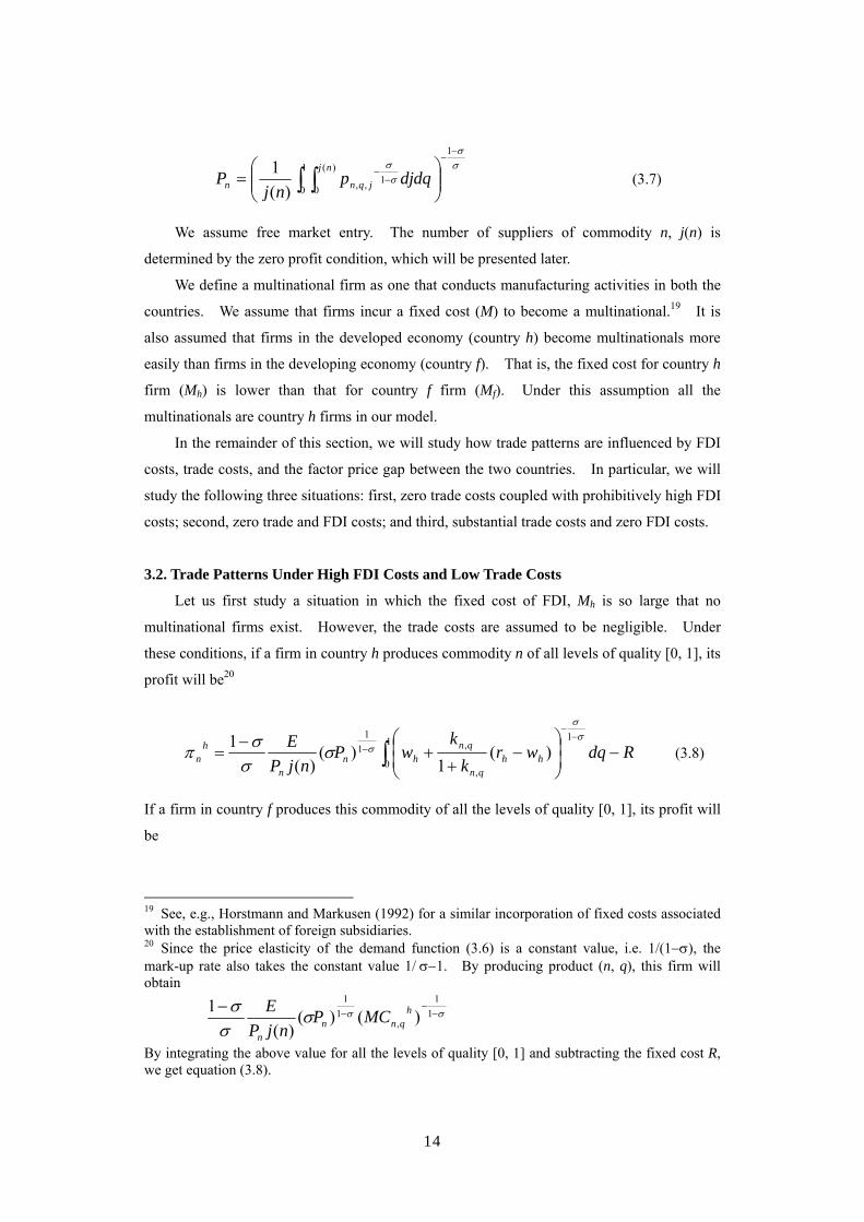
3.2. Trade Patterns Under High FDI Costs and Low Trade Costs

Let us first study a situation in which the fixed cost of FDI, Mh is so large that no

multinational firms exist. However, the trade costs are assumed to be negligible. Under

these conditions, if a firm in country h produces commodity n of all levels of quality [0, 1], its

profit will be20

Rdqwrk

kwP

njPE

hhqn

qnhn

n

hn −

−

++

−= ∫

−−

−1

0

1

,

,11

)(1

)()(

1 σσ

σσσ

σπ (3.8)

If a firm in country f produces this commodity of all the levels of quality [0, 1], its profit will

be

19 See, e.g., Horstmann and Markusen (1992) for a similar incorporation of fixed costs associated with the establishment of foreign subsidiaries. 20 Since the price elasticity of the demand function (3.6) is a constant value, i.e. 1/(1−σ), the mark-up rate also takes the constant value 1/ σ−1. By producing product (n, q), this firm will obtain

σσσσ

σ −−

−− 11

,1

1

)()()(

1 hqnn

n

MCPnjP

E

By integrating the above value for all the levels of quality [0, 1] and subtracting the fixed cost R, we get equation (3.8).

15

Rdqwrk

kwP

njPE

ffqn

qnfn

n

fn −

−

++

−= ∫

−−

−1

0

1

,

,11

)(1

)()(

1 σσ

σσσ

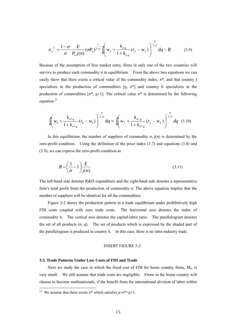
σπ (3.9)

Because of the assumption of free market entry, firms in only one of the two countries will

survive to produce each commodity n in equilibrium. From the above two equations we can

easily show that there exists a critical value of the commodity index, n*, and that country f

specializes in the production of commodities [n, n*] and country h specializes in the

production of commodities [n*, n+1]. The critical value n* is determined by the following

equation.21

∫∫−

−−

−

−

++=

−

++

1

0

1

*,

*,1

0

1

*,

*, )(1

)(1

dqwrk

kwdqwr

kk

w ffqn

qnfhh

qn

qnh

σσ

σσ

(3.10)

In this equilibrium, the number of suppliers of commodity n, j(n) is determined by the

zero-profit condition. Using the definition of the price index (3.7) and equations (3.8) and

(3.9), we can express the zero-profit condition as

)(

11nj

ER

−=

σ (3.11)

The left-hand side denotes R&D expenditure and the right-hand side denotes a representative

firm’s total profit from the production of commodity n. The above equation implies that the

number of suppliers will be identical for all the commodities.

Figure 3-2 shows the production pattern in a trade equilibrium under prohibitively high

FDI costs coupled with zero trade costs. The horizontal axis denotes the index of

commodity n. The vertical axis denotes the capital-labor ratio. The parallelogram denotes

the set of all products (n, q). The set of products which is expressed by the shaded part of

the parallelogram is produced in country h. In this case, there is no intra-industry trade.

INSERT FIGURE 3-2

3.3. Trade Patterns Under Low Costs of FDI and Trade

Next we study the case in which the fixed cost of FDI for home country firms, Mh, is

very small. We still assume that trade costs are negligible. Firms in the home country will

choose to become multinationals, if the benefit from the international division of labor within 21 We assume that there exists n* which satisfies n<n*<n+1.

16

the firm is greater than the fixed cost of the FDI. They will produce high-quality products,

of which the capital-labor ratio is greater than k* in country h, and produce low-quality

products, of which the capital-labor ratio is smaller than k*, in country f. This FDI is

“vertical” in the sense that manufacturing affiliates are established in order to take advantage

of cheap labor and a large part of the output is exported to the multinational’s home country.

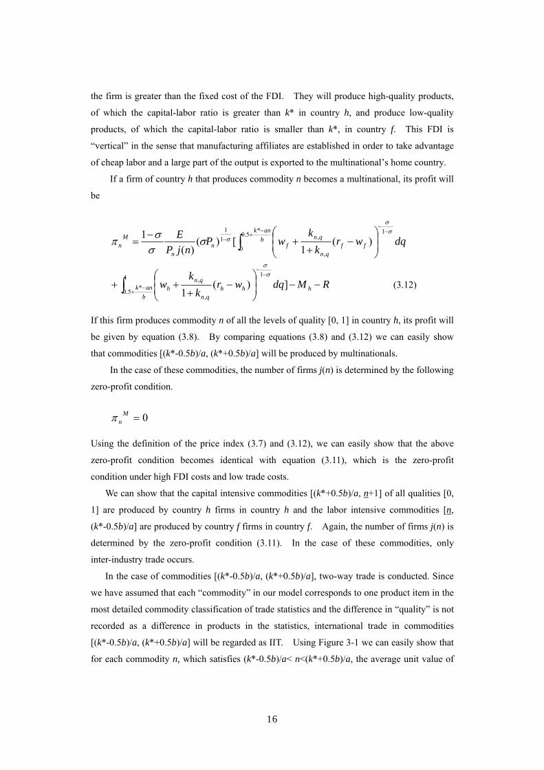
If a firm of country h that produces commodity n becomes a multinational, its profit will

be

∫−

+ −−

−

−

++

−= b

ank

ffqn

qnfn

n

Mn dqwr

kk

wPnjP

E *5.0

0

1

,

,11

)(1

[)()(

1 σσ

σσσ

σπ

RMdqwrk

kw h

bank hh

qn

qnh −−

−

+++ ∫ −

+

−−

])(1

1*5.0

1

,

,σ

σ

(3.12)

If this firm produces commodity n of all the levels of quality [0, 1] in country h, its profit will

be given by equation (3.8). By comparing equations (3.8) and (3.12) we can easily show

that commodities [(k*-0.5b)/a, (k*+0.5b)/a] will be produced by multinationals.

In the case of these commodities, the number of firms j(n) is determined by the following

zero-profit condition.

0=M

nπ Using the definition of the price index (3.7) and (3.12), we can easily show that the above

zero-profit condition becomes identical with equation (3.11), which is the zero-profit

condition under high FDI costs and low trade costs.

We can show that the capital intensive commodities [(k*+0.5b)/a, n+1] of all qualities [0,

1] are produced by country h firms in country h and the labor intensive commodities [n,

(k*-0.5b)/a] are produced by country f firms in country f. Again, the number of firms j(n) is

determined by the zero-profit condition (3.11). In the case of these commodities, only

inter-industry trade occurs.

In the case of commodities [(k*-0.5b)/a, (k*+0.5b)/a], two-way trade is conducted. Since

we have assumed that each “commodity” in our model corresponds to one product item in the

most detailed commodity classification of trade statistics and the difference in “quality” is not

recorded as a difference in products in the statistics, international trade in commodities

[(k*-0.5b)/a, (k*+0.5b)/a] will be regarded as IIT. Using Figure 3-1 we can easily show that

for each commodity n, which satisfies (k*-0.5b)/a< n<(k*+0.5b)/a, the average unit value of

17

developed country h’s exports is higher than the average unit value of developing country f ’s

exports. Intra-industry trade with a vertical division of labor occurs for these commodities.

Figure 3-3 shows the production pattern when the costs of FDI and trade are very small.

Under these circumstances, the share of vertical IIT in total trade is large. The products

expressed by the parallelogram efgh are subject to vertical IIT while the products expressed

by the two parallelograms, abfe and hgcd are subject to inter-industry trade.

Under very low costs of FDI and trade, country h specializes more in the production of

the capital-intensive products than would be the case with high FDI costs (Figure 3-2).

What is more, VIIT caused by FDI reduces the demand for labor in country h and the demand

for capital in country f.

INSERT FIGURE 3-3

If the fixed cost of FDI, Mh, is not negligible, the set of commodities that are produced

by multinationals will be smaller. In the case of commodities that are included in the set

[(k*-0.5b)/a, (k*+0.5b)/a] but close to the border values (k*-0.5b)/a or (k*+0.5b)/a, gains

from the international division of labor within a firm are surpassed by FDI costs and firms do

choose not to become a multinational. If there exist substantial costs of FDI, the set of

commodities subject to VIIT will be narrower than the corresponding set in the case of

negligible FDI costs.22 And the share of vertical IIT in total trade will become smaller than

that in the case of negligible FDI costs.

It is important to note that if the factor-price gap between the two countries is small, then

firms will have limited incentive to engage in the international division of labor through FDI

and the set of commodities subject to VIIT will become narrower. For example, if the two

countries have almost identical factor prices, even relatively small FDI costs will stifle

vertical FDI and vertical IIT.

3.4. Trade Patterns Under Low FDI Costs and High Trade Costs

Next, let us study the effects of trade costs. In order to keep our analysis tractable, we

assume again that FDI costs for firms in country h, Mh, are negligible. Let Th, f denote one

plus the cost factor of trading products from country h to country f. Moreover, for the time

being, we assume that Tf, h, the cost factor of trading products in the reverse direction from

country f to country h, is zero. Under these assumptions, firms from country h will have an

22 More rigorously, we should note that the increase of the number of multinational firms will cause a decline in Pn and reduce the incentive for firms to become a multinational. Therefore, at a certain value of n multinational firms and non-multinational firms co-exist.

18

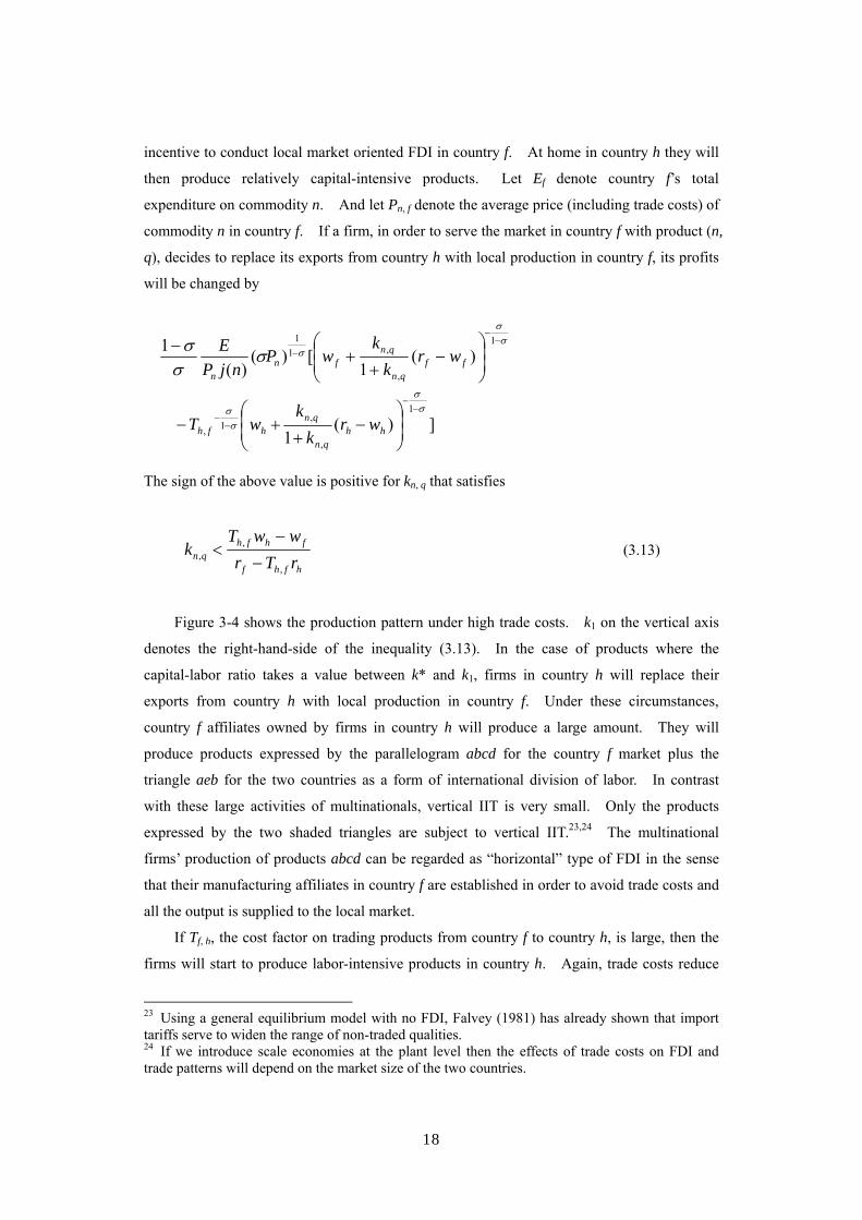
incentive to conduct local market oriented FDI in country f. At home in country h they will

then produce relatively capital-intensive products. Let Ef denote country f’s total

expenditure on commodity n. And let Pn, f denote the average price (including trade costs) of

commodity n in country f. If a firm, in order to serve the market in country f with product (n,

q), decides to replace its exports from country h with local production in country f, its profits

will be changed by

σσ

σσσ

σ −−

−

−

++

− 1

,

,11

)(1

[)()(

1ff

qn

qnfn

n

wrk

kwP

njPE

])(1

1

,

,1,

σσ

σσ −

−

−−

−

++− hh

qn

qnhfh wr

kk

wT

The sign of the above value is positive for kn, q that satisfies

hfhf

fhfhqn rTr

wwTk

,

,, −

−< (3.13)

Figure 3-4 shows the production pattern under high trade costs. k1 on the vertical axis

denotes the right-hand-side of the inequality (3.13). In the case of products where the

capital-labor ratio takes a value between k* and k1, firms in country h will replace their

exports from country h with local production in country f. Under these circumstances,

country f affiliates owned by firms in country h will produce a large amount. They will

produce products expressed by the parallelogram abcd for the country f market plus the

triangle aeb for the two countries as a form of international division of labor. In contrast

with these large activities of multinationals, vertical IIT is very small. Only the products

expressed by the two shaded triangles are subject to vertical IIT.23,24 The multinational

firms’ production of products abcd can be regarded as “horizontal” type of FDI in the sense

that their manufacturing affiliates in country f are established in order to avoid trade costs and

all the output is supplied to the local market.

If Tf, h, the cost factor on trading products from country f to country h, is large, then the

firms will start to produce labor-intensive products in country h. Again, trade costs reduce

23 Using a general equilibrium model with no FDI, Falvey (1981) has already shown that import tariffs serve to widen the range of non-traded qualities. 24 If we introduce scale economies at the plant level then the effects of trade costs on FDI and trade patterns will depend on the market size of the two countries.

19

vertical IIT substantially.

INSERT FIGURE 3-4

The main results of our theoretical analysis can be summarized as follows.

(1) Vertical intra-industry trade is a fragile flower, which flourishes only when both FDI costs

and trade costs are small. If there exist substantial FDI costs, gains from the

international division of labor within firms will be surpassed by FDI costs; firms in the

developed country will not conduct “vertical” FDI which, in our model, is indispensable

for vertical IIT. If it is very costly to trade products from the developed country to the

developing country, then firms in the developed country will replace their exports from

their home country with local production in the developing country. Because of this

“horizontal” FDI, vertical IIT becomes very small.

(2) If there exist substantial costs of FDI, the share of vertical IIT in total trade will depend

on the factor price gap between the two countries. If the factor price gap is small, then

firms will have limited incentive to engage in the international division of labor through

FDI, and vertical IIT will become small.

4. An Econometric Analysis of the Determinants of Japan’s Intra-Industry Trade

4.1. The Method of Estimation

So far we have seen that vertical IIT has been rapidly growing in importance in the East

Asian countries. As described in the previous section, perhaps FDI is an important

determinant of vertical IIT.

In the past twenty years, a number of studies have empirically tested for country- and

industry-specific influences on intra-industry trade (for example, Balassa 1986, Balassa and

Bauwens 1987, Bergstrand 1990, Stone and Lee 1995, etc.). However, most of the previous

results, using Grubel-Lloyd intra-industry trade indexes, do not distinguish between

horizontal and vertical IIT even though theory suggests their determinants will differ. More

recently, Greenaway, Hine and Milner (1994, 1995), Fontagné, Freudenberg and Péridy

(1997), Durkin and Krygier (2000), and others did make such a distinction in their data and

tested for the determinants of horizontal and vertical IIT separately, employing a methodology

which builds on the work of Abd-el-Rahman (1991).25 Examining the trade of the UK with

25 In addition to the studies listed above, Aturupane, Djankov and Hoekman (1999) analyze the determinants of vertical and horizontal IIT between the EU and Central and Eastern European transition economies, while Hu and Ma (1999) focus on China, making a distinction between vertical and horizontal IIT.

20

62 countries in the year 1988, Greenaway, Hine and Milner (1994) focus on whether the

pattern of IIT was related to country-specific factors and find that both market size and

membership of a customs union are relevant to the explanation of the pattern of vertical IIT.

In their results, however, relative factor endowments do not seem to support the neo-factor

proportions model. Their results seemed to accord with Linder-type trade. That is, their

results suggest that much vertical IIT arises from similarities in tastes among consumers

across different countries rather than from differential endowments of capital and labor. On

the other hand, Durkin and Krygier (2000), examining US bilateral IIT with 20 OECD trading

partners for the years 1989-92, find evidence of a positive and significant relationship

between differences in GDP per capita and the share of vertical IIT. Contrary to the results

of Greenaway, Hine and Milner (1994), the findings of Durkin and Krygier (2000) support the

view that IIT may be positively related to differences in relative wages and, to the extent that

differences in GDP per capita and relative wages are correlated, differences in per capita

GDP.26

Fontagné, Freudenberg and Péridy (1997) construct a four-dimensional panel data set

(i.e. time, industry, reference countries and partner countries) on intra-EC vertical and

horizontal IIT for the period from 1980 to 1994, and conduct an econometric analysis of the

determinants of IIT. They find that the difference in factor endowments between countries,

proxied by the difference in per capita income, reduces horizontal IIT but increases vertical

IIT. Moreover, they include an indicator of bilateral FDI, a proxy for the in-depth

integration of economies, as an explanatory variable, and find that FDI leads to greater trade

in both vertical and horizontal IIT.

Although some of these studies mentioned the importance of FDI and mostly found a

positive relationship between FDI and IIT, the mechanism of how FDI has enhanced the

international division of labor and consequently increased IIT has not been well explained and

adequately examined. Moreover, as for vertical and horizontal IIT in Asia, hardly any

comprehensive empirical studies have been conducted although many researchers have been

investigating total IIT (not making a distinction between vertical and horizontal IIT). A rare

exception is Hu and Ma’s (1999) study on China, in which the dependent variable, the

bilateral vertical/horizontal IIT index, is aggregated over industrial groups of SITC 3, 6, 7,

and 8. By examining bilateral trade with 45 countries, the study finds a significant positive

26 Durkin and Krygier (2000) explain that their regression results differ from those in Greenaway, Hine and Milner (1994) because: 1) the sample in Greenaway, Hine and Milner (1994) includes some developing as well as developed countries; 2) the absolute levels of GDP enter slightly differently as regressors; and 3) Greenaway, Hine and Milner (1994) do not run fixed-effects regressions.

21

relationship between FDI and vertical IIT. However, the FDI variable used in their study is

the total amount of China’s inward FDI from the partner countries, not inward FDI data by

industry.27 Analyses using industry-level FDI data have been extremely difficult because of

the limited data availability for Asian countries.

In this section, we test for the determinants of bilateral vertical IIT between Japan and

her 43 major trading partners for the period from 1988 to 2000, taking the electrical

machinery industry as a case.28 Because of the limitations of the PC-TAS data mentioned in

Section 2, Japan’s bilateral trade data at the 9-digit HS88 level provided by the Ministry of

Finance (MOF) are used for the econometric analysis, which allows us to cover a much longer

period and more partner countries.29 As argued in Section 2.5, vertical IIT in Japan’s trade

with China and the ASEAN economies in electrical and machinery products has been growing

rapidly in recent years. At the same time, the Japanese electrical machinery industry has

been vigorously pursuing FDI and is characterized by an active international division of labor.

Given that China and the ASEAN countries are among the largest recipients of Japanese FDI,

we would expect FDI to be a major driving force behind the increase in vertical IIT as shown

in the theoretical analysis in the previous section. Thus, the hypotheses formulated in

Section 3 are tested using the following equations:

Ykk’t = α0 + α1 FDIkk’t + α2 DGDPPCkk’t + α3 DISTkk’ + α4 INDSIZEkk’t

+ α5 DREGk + α6 Dt + εkk’t (4.1)

where

ykk’t = SHVIIT, LTSHVIIT

FDIkk’t : foreign direct investment

DGDPPC kk’t : comparative advantage (and human capital)

DISTkk’: geographic distance

INDSIZE kk’t: size of the industry

27 The total amount of FDI includes investment in natural resource seeking and/or in sales establishments, etc. Although it is certainly more appropriate to use industry-level FDI data to capture the size of activities in each industry, there are no comprehensive FDI data by industry and by country for Asian countries. 28 The list of the forty-three countries used in the regression analysis is presented in Appendix Table C1. Japan’s trading partners included in the econometric analysis are limited to these forty-three countries based on the availability of data for constructing explanatory and instrumental variables. 29 As the Japanese trade data provided by MOF include quantity data for most HS 9-digit products, the coverage of products used for the calculation of IIT indexes becomes much wider than with the PC-TAS data. However, an important deficiency of the MOF trade data is that exports are recorded on an f.o.b. basis while imports are on a c.i.f. basis. For details on our methodology of adjusting for the discrepancy between f.o.b. and c.i.f., see Section 2.

22

DREGk: region dummies

Dt: year dummies

Subscript t denotes year t.

The variables used in this estimation are defined in Table 4-1. Further details on the

definitions and sources of the variables are provided in Appendix C. As dependent variables

we use the shares of vertical intra-industry trade (SHVIIT) between countries k and k’ (Japan),

which are defined in Section 2. Since our dependent variable SHVIIT is limited in range

between zero and one, we will mainly use the logistic transformations of SHVIIT, denoted by

LTSHVIIT, as our dependent variable. In line with our procedure so far, the regression

analysis in this section is mainly conducted using a 25% threshold to distinguish between

vertically and horizontally differentiated products.30

We mainly consider the following four factors as determinants of SHVIIT:

(1) FDIkk’t. This measures the activity of Japanese-affiliated firms in the electrical

machinery industry in country k. As shown in Section 3, we expect that the expansion

of the activities by Japanese-affiliated firms might be associated with an increase in

vertical IIT. We employ the variable FDISALEkk’t as a proxy for the extent of the

activity of Japanese-affiliated firms. The variable is defined as the ratio of the sales by

Japanese-affiliated firms in country k to domestic output in Japan for the electrical

machinery industry. We also include an interaction term of FDISALEkk’t and a variable

representing the degree of trade friction between the two countries (TRFRC) in order to

distinguish FDI for the purpose of avoiding trade friction from FDI aimed at the

international division of labor.

(2) The difference in per capita GDP (DGDPPCkk’t), which is defined as the absolute value

of the difference in per capita GDP between country k and k’ (Japan). In our theoretical

model presented in Section 3, vertical differentiation is explicitly modeled as differences

in quality between similar products. In the case where two countries have differential

endowments of capital and labor, it is assumed that the higher quality variety of the

differentiated good is produced using relatively capital-intensive techniques. As a

result, the higher income, relatively capital-abundant country specializes in relatively

high-quality manufactures, while the lower income, relatively labor-abundant country

specializes in low-quality manufactures. Therefore, we predict that the share of vertical

IIT in the bilateral trade of a pair of countries will be greater the greater the difference in

30 To test the sensitivity of our results, the regression analysis was also repeated using a 15% threshold. The regression result is presented in Appendix Table C2.

23

the capital-labor endowment of the two countries and, accordingly, the greater the

difference in per capita GDP. In addition to our basic model, we estimate some

additional models which include DGDPPCkk’t squared as an explanatory variable, taking

non-linearity into account. Moreover, differences in human capital accumulation

between country k and Japan, DEDUYRkk’, is also included as an explanatory variable.

DEDUYRkk’ is defined as the absolute value of the gap in average years of schooling

between country k and Japan. Since vertical IIT is determined by quality factors, we

believe that the human capital intensity would be one of the most important factors

influencing this type of intra-industry trade. A larger difference in human capital

intensity would result in a larger difference in the price (quality) of the product.

Therefore, vertical IIT will increase.

(3) The geographical distance between the capital city of country k and Tokyo, DIST kk’.

The distance between producers should lead to a reduction in two-way trade for goods

subject to transportation costs. In the case of vertical FDI, the distance between the

parent firm and its subsidiaries should hinder them from creating an efficient production

network and from communicating smoothly. Therefore, the distance should reduce

vertical FDI, resulting in a reduction of vertical IIT. Consequently, it is to be expected

that this variable will have a negative impact.

(4) The size of the electrical machinery industry in country k, INDSIZE kk’. It may be

presumed that with the size of the industry in country k, the volume of trade will increase.

Therefore, we expect a positive coefficient for this variable.

As FDI variables are endogenously determined, equation (4.1) is estimated by

instrumental variables (IV) regression with linear specifications.

INSERT TABLE 4-1

4.2 Regression Results

The main results of the regression analysis for the determinants of vertical IIT between

Japan and her major trading partners are presented in Table 4-2.31 In general, they strongly

support the hypothesis that FDI measured by the sales amount is a major determinant of

31 We also estimated the model by IV regression with samples for which outliers are excluded (we define outliers as observations which exceed the range of mean ±2.5*standard deviation) and the model by the ordinary least squares (OLS) method. Moreover, we conducted a three-stage least squares estimation for a system of simultaneous equations. These results are reported in Appendix Tables C2 and C3, respectively; we obtain very similar results to those in Table 4.2.

24

vertical IIT. The coefficient on FDISALE is positive and strongly significant in all the

equations in Table 4-2. Moreover, the interaction term of trade friction and FDI

(TRFRC*FDISALE) has, as expected, a significant negative coefficient in all cases. The

geographical distance (DIST) also has a significant negative coefficient in all the equations as

expected, which suggests that geographical distance raises the transportation and transaction

costs between the countries and should lead to a reduction in IIT. The size of the electrical

machinery industry (INDSIZE) has the expected positive sign in most cases but is not

statistically significant. As for the difference in factor endowments, contrary to our

prediction, the difference in per capita GDP (DGDPPC) has a negative coefficient in most of

the equations, implying that the share of VIIT will be smaller the greater difference in factor

endowments. This result is similar to that in Greenaway, Hine and Milner (1994), although

it is inconsistent with the results of the study by Durkin and Krygier (2000) on US IIT with

OECD countries and the study by Fontagné, Freudenberg and Péridy (1997) on the EC

countries. However, looking at the coefficients on DGDPPC squared in equations (4) and

(5) in Table 4-2, we can see that the greater the difference in per capita GDP the greater will

be the share of VIIT in the case of bilateral trade with countries of which per capita GDP

differs from Japan’s per capita GDP by more than approximately 10,000 international dollars.

Therefore, in the case of Japan’s bilateral vertical IIT in the electrical machinery industry with

lower income countries (where the difference in per capita GDP with Japan is more than

10,000 international dollars), this result may imply that relative factor endowments support

the Heckscher-Ohlin-type neo-factor proportions hypothesis rather than the Linder-type

demand-similarity hypothesis after controlling for the level of FDI and for region-specific

effects. In addition to these results, the difference in human capital accumulation

(DEDUYR) does not have a significant impact on vertical IIT.

INSERT TABLE 4-2

5. Conclusions

In this paper, we investigated the recent change in trade patterns in East Asia and

compared these patterns with those in EU, using the HS 6-digit level data published by the

United Nations and the HS 9-digit level data provided by the Ministry of Finance of Japan.

Specifically, we aimed to establish whether the intra-regional trade in East Asia is of an

“inter-industry,” “vertical intra-industry,” or “horizontal intra-industry” nature. We also

analyzed the role of FDI in the change of trade patterns. Our analysis reveals that, although

still much lower than in the EU, intra-industry trade, and particularly vertical IIT, in East Asia

25

has grown rapidly in importance in overall intra-regional trade. This is especially the case in

the electrical machinery industry and the general and precision machinery industry.

Moreover, while for most EU countries, the share of IIT remained almost constant during the

period from 1996 to 2000, it expanded quickly for East Asian countries. According to our

calculations, the share of vertical IIT in total intra-East Asian trade grew from 16.6% in 1996

to 23.7% in 2000, while that in total intra-EU trade increased only slightly from 37.5% to

40.0% during the same period.

Taking into account that the share of vertical IIT in the electrical machinery industry

has increased dramatically in East Asia, we also conducted a more detailed analysis of this

industry, using Japan’s bilateral trade data at the HS 9-digit level. Most interestingly,

vertical IIT has risen dramatically in Japan’s trade with China and many of the ASEAN

countries. This increase in vertical IIT with these countries seems to have a strong positive

correlation with the extent of the activities by Japanese electrical machinery MNEs.

Our theoretical examination suggests that if the fixed cost of FDI is relatively small,

firms choose to become multinational and exploit the factor price gap between the home base

and foreign countries. As a result, MNE’s home country specializes more in the production

of capital-intensive high-quality products, while the host country specializes more in the

production of labor-intensive low-quality products. Similarly, the lower the trade costs, the

more vertical IIT will occur between the home and the host countries. Therefore, our

theoretical analysis implies that lower costs of FDI and trade enable firms to benefit from the

international vertical division of labor, resulting in an increase in vertical IIT.

Taking the descriptive and theoretical analyses as a cue, we then conducted an

econometric investigation to test for the determinants of IIT, taking Japan’s bilateral trade in

the electrical machinery industry as a case. We found that FDI has a strongly positive

impact on vertical IIT. Moreover, we also found a significantly negative impact of the

geographical distance on vertical IIT, suggesting that the higher the trade costs, the less

vertical IIT is there likely to occur. As for differences in factor endowments, contrary to our

prediction, the results suggest that VIIT will be lower the greater the differences in factor

endowments are. However, we also found that the difference in factor endowments

increases VIIT when the gap in per capita GDP with Japan exceeds 10,000 international

dollars (many Asian countries fall into this category) after controlling for the level of FDI and

for region-specific effects. In other words, in the case of trade with lower income countries,

including many Asian countries, the results support a Heckscher-Ohlin-type neo-factor

proportions hypothesis.

Overall, the results imply that in the East Asian region FDI played a significant role in

26

the rapid increase of vertical IIT in recent years. Moreover, we found that the largest part of

total IIT growth in the region is attributable to the growth of vertical and not of horizontal IIT.

Many economists have studied the impact of Japan’s direct investment abroad on Japan’s

industrial structure and factor markets as a consequence of the resulting imports from the rest

of East Asia.32 However, there is almost no empirical study on how the increase in vertical

IIT has changed the industrial structure and factor prices in Japan. We would like to study

this issue in near future.

32 For example, see Head and Ries (2000), Tomiura (2001), Kimura (2001), Kimura and Fukasaku (2001), and Kwan (2002).

27

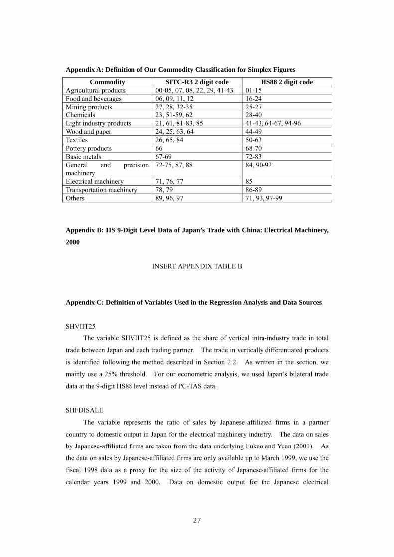
Appendix A: Definition of Our Commodity Classification for Simplex Figures

Commodity SITC-R3 2 digit code HS88 2 digit code Agricultural products 00-05, 07, 08, 22, 29, 41-43 01-15 Food and beverages 06, 09, 11, 12 16-24 Mining products 27, 28, 32-35 25-27 Chemicals 23, 51-59, 62 28-40 Light industry products 21, 61, 81-83, 85 41-43, 64-67, 94-96 Wood and paper 24, 25, 63, 64 44-49 Textiles 26, 65, 84 50-63 Pottery products 66 68-70 Basic metals 67-69 72-83 General and precision machinery

72-75, 87, 88 84, 90-92

Electrical machinery 71, 76, 77 85 Transportation machinery 78, 79 86-89 Others 89, 96, 97 71, 93, 97-99

Appendix B: HS 9-Digit Level Data of Japan’s Trade with China: Electrical Machinery,

2000

INSERT APPENDIX TABLE B

Appendix C: Definition of Variables Used in the Regression Analysis and Data Sources

SHVIIT25

The variable SHVIIT25 is defined as the share of vertical intra-industry trade in total

trade between Japan and each trading partner. The trade in vertically differentiated products

is identified following the method described in Section 2.2. As written in the section, we

mainly use a 25% threshold. For our econometric analysis, we used Japan’s bilateral trade

data at the 9-digit HS88 level instead of PC-TAS data.

SHFDISALE

The variable represents the ratio of sales by Japanese-affiliated firms in a partner

country to domestic output in Japan for the electrical machinery industry. The data on sales

by Japanese-affiliated firms are taken from the data underlying Fukao and Yuan (2001). As

the data on sales by Japanese-affiliated firms are only available up to March 1999, we use the

fiscal 1998 data as a proxy for the size of the activity of Japanese-affiliated firms for the

calendar years 1999 and 2000. Data on domestic output for the Japanese electrical

28

machinery industry are taken from Elsevier Advanced Technology/Reed Electronics Research

(various years), Yearbook of World Electronics Data.

DGDPPC

The variable DGDPPC is defined as the absolute difference in per capita GDP between

country k and Japan (k’). The per capita GDP data (in current thousands of international

dollars) are taken from World Bank (2002b), World Development Indicators 2002, CD-ROM.

For countries for which data on GDP per capita in current international dollars are not

available in World Bank (2002b), we estimated the data using other data sources as follows:

first, we multiplied the ratio of the country’s GDP to Japan’s GDP calculated in current

international dollars from International Monetary Fund (various years) by estimates of Japan’s

GDP in current international dollars from World Bank (2002b). Then, we divided it by

population estimates from World Bank (2002b).

DEDUYR

The variable DEDUYR is the absolute difference in average years of total schooling of

the total population as of 1990 between country k and Japan, which is a proxy for the

difference in human capital endowment between country k and Japan. The data are taken

from World Bank (2002a), Barro-Lee Dataset: International Schooling Years and Schooling

Quality, (downloaded from www.worldbank.org on 18 September, 2002). For Nigeria and

Saudi Arabia, where data on average years of total schooling were not available, we estimated

the value of this variable as follows: first, for all the countries where the schooling data are

available, we regressed the average years of total schooling on GDPPC (per capita GDP),

GDP, and regional dummies. Then, using the estimated equation, we estimated the

theoretical value of average years of schooling for those countries.

DIST

The variable DIST is the logarithm of the geographical distance expressed in 1,000

kilometers between the capital city of country k and Tokyo.

INDSIZE

The variable INDSIZE is the size of the electrical machinery industry in country k

normalized by the size of the industry in Japan. The data are taken from Elsevier Advanced

Technology/Reed Electronics Research (various years), Yearbook of World Electronics Data.

29

GDP

GDP is an indicator of the size of the economies under study. The data on GDP in

current international dollars are taken from World Bank (2002b), World Development

Indicators 2002, CD-ROM. For countries for which data on GDP in current international

dollars are not available in World Bank (2002b), we estimated the data multiplying the ratio of

the country’s GDP to Japan’s GDP calculated in current international dollars from

International Monetary Fund (various years) by estimates of Japan’s GDP in current

international dollars from World Bank (2002b).

RISK

The variable RISK is a proxy for country k’s risk of default. The data are taken from

Institutional Investor Systems, Institutional Investor, various years.

COTAX

COTAX is the effective corporate tax rate for country k for the year 1993. The data

are taken from Fukao and Yue (1997). For Denmark, Finland, Hungary, and Poland, where

the effective corporate tax rate was not available, the legal corporate tax rate is used.

OPERATE1

The variable OPERATE1 is the first principal component of the conditions for

obtaining an operation permission. The data are taken from Fukao and Chung (1996). For

Denmark, Finland, Hungary, and Poland, where OPERATE1 data were not available, we

estimated the value of this variable as follows: first, for all the countries where OPERATE1

data are available, we regressed the first principal component of the conditions for obtaining

an operation permission on GDPPC (per capita GDP), GDP, EDUYR (average years of total

schooling of the total population), and regional dummies. Then, using the estimated

equation, we estimated the theoretical value of OPERATE1 for those countries.

OPERATE2

The variable OPERATE2 is the second principal component of the conditions for

obtaining an operation permission. The data are taken from Fukao and Chung (1996). For

Denmark, Finland, Hungary, and Poland, where OPERATE2 data were not available, we

estimated the value of this variable as follows: first, for all the countries where OPERATE2

30

data are available, we regressed the second principal component of the conditions for

obtaining an operation permission on GDPPC (per capita GDP), GDP, EDUYR (average

years of total schooling of the total population), and regional dummies. Then, using the

estimated equation, we estimated the theoretical value of OPERATE2 for those countries.

TRFRC

The variable TRFRC is a measure of the extent of FDI undertaken to avoid trade

friction with country k defined as:

(Number of Japanese-affiliated firms who answered that trade friction was one of the

motivations behind establishing an affiliate in country k) / (total number of Japanese-affiliated

firms in country k)

The data are taken from Fukao and Chung (1996).

INSERT APPENDIX TABLES C1, C2, and C3

31

References Abe, Shigeyuki (1997) “Trade and Investment Relations of Japan and ASEAN in a Changing

Global Economic Environment,” Kobe Economic and Business Review, vol. 42, pp. 11-54.

Abd-el-Rahman, K. (1991) “Firms’ Competitive and National Comparative Advantages as Joint Determinants of Trade Composition,” Weltwirtschaftliches Archiv, vol. 127, No.1, pp. 83-97.

Aturupane, Chonira, Simeon Djankov and Bernard Hoekman (1999) “Horizontal and Vertical Intra-Industry Trade between Eastern Europe and the European Union,” Weltwirtschaftliches Archiv, Vol.135, No.1, pp. 62-81.

Balassa, Bela (1986) “The Determinants of Intra-Industry Specialisation in US Trade,” Oxford Economic Papers, 38, pp. 220-233.

Balassa, Bela and Luc Bauwens (1987) “Intra-Industry Specialization in a Multi-Country and Multi-Industry Framework,” Economic Journal 97(December), pp. 923-939.

Bergstrand, Jeffrey H. (1990) “The Heckscher-Ohlin-Samuelson Model, The Linder Hypothesis and the Determinants of Bilateral Intra-Industry Trade,” Economic Journal, 100(December), pp. 1216-1229.

Carr, David L., James R. Markusen, and Keith E. Maskus, (2001) “Estimating the Knowledge-Capital Model of the Multinational Enterprise,” American Economic Review, Vol. 91, No. 3, pp. 693-708.

Durkin, John T. and Markus Krygier (2000) “Differences in GDP Per Capita and the Share of Intraindustry Trade: The Role of Vertically Differentiated Trade,” Review of International Economics, 8(4), pp. 760-774.

Elsevier Advanced Technology/Reed Electronics Research (various years), Yearbook of World Electronics Data.

Falvey, Rodney E. (1981) “Commercial Policy and Intra-Industry Trade,” Journal of International Economics, 11, pp. 495-511.

Feenstra, Robert C. and Gordon H. Hanson (1996) “Foreign Investment, Outsourcing, and Relative Wages” in Robert C. Feenstra, Gene M. Grossman and Douglas A. Irwin (eds.), The Political Economy of Trade Policy: Papers in Honor of Jagdish Bhagwati, Cambridge, Mass: The MIT Press.

Feenstra, Robert C. and Gordon H. Hanson (2001) “Global Production Sharing and Rising Inequality: A Survey of Trade and Wages,” NBER Working Paper No. 8372, July, National Bureau of Economic Research.

Fontagné, Lionel, Michael Freudenberg, and Nicholas Péridy (1997) “Trade Patterns Inside the Single Market,” CEPII Working Paper No. 1997-07, April, Centre D’Etudes Prospectives et D’Informations Internationales. Retrieved from [http://www.cepii.fr/anglaisgraph/workpap/pdf/1997/wp97-07.pdf] 7 June 2002.

Fukao, Kyoji, and Hoon Chung (1996) “Chokusetsu Toshi Sakikoku no Kettei Yoin Nitsuite: Wagakuni Seizogyo Nikan Suru Jisho Bunseki (On the Determinants of the Location Decision in Direct Investment Abroad: An Empirical Analysis on Japan’s Manufacturing Industry),” Financial Review, No.38, Policy Research Institute, Ministry of Finance,Japan, February 1996.

Fukao, Kyoji and Tangjun Yuan (2001) “Kohyo Data no Paneruka to Naigaiso niyoru Kaigai Jigyo Katsudo Kihon-Doko Chusa no Boshudan Suikei: 1985-1998 (Estimation of Business Activities by All the Foreign Affiliates of Japanese Firms based on Micro-panel-data of METI Survey: 1985-1998),” Kaigai Jigyo Katudo Doko Chosa, Gaisikei Kigyo Katsudo no Doko Data Nadoni Motozuku Bunseki Kenkyu (Studies based on METI Survey on Foreign Affiliates of Japanese Firms and Survey on Japanese Affiliates of Foreign Firms), edited by Institute for International Trade and Investment, Tokyo, Japan.

Fukao, Kyoji and Ximing Yue (1997) “Denki Meika no Ricchi Sentaku (Location Decisions

32

of Japan’s Electric Machinery Firms),” Mita Journal of Economics, (in Japanese) The Keio Economic Society, Keio University.

Greenaway, D., R.Hine, and C.Milner (1994) “Country-Specific Factors and the Pattern of Horizontal and Vertical Intra-Industry Trade in the UK,” Weltwirtschaftliches Archiv, Vol.130, No.1, pp.77-100.

Greenaway, D., R.Hine, and C.Milner (1995) “Vertical and Horizontal Intra-Industry Trade: A Cross Industry Analysis for the United Kingdom,” Economic Journal, Vol.105, November, pp.1505-1518.

Head, Keith and John Ries (2000) “Offshore Production and Skill Upgrading by Japanese Manufacturing Firms,” mimeo, University of British Columbia.

Helpman, Elhanan and Paul R. Krugman (1985) Market Structure and Foreign Trade: Increasing Returns, Imperfect Competition, and the International Economy, Cambridge, MA: The MIT Press.

Horstmann, Ignatius J. and James R. Markusen (1992) “Endogenous Market Structures in International Trade (Natura Facit Saltum),” Journal of International Economics, vol. 32, pp.109-129.

Hu, Xiaoling and Yue Ma (1999) “International Intra-Industry Trade of China,” Weltwirtschaftliches Archiv, vol. 135, No. 1, pp.82-101.

International Monetary Fund (2002) International Financial Statistics, June 2002, CD-ROM. International Monetary Fund (various years), World Economic Outlook and the database

underlying the September 2002 issue, Washington, D.C.: International Monetary Fund (downloaded on October 17, 2002 from IMF web site, http://www.imf.org/external/pubs/ft/weo/2002/02/data/index.htm).

Ishida, Osamu (2002) “Nihon no Sangyonai Boeki no Kozo (Structure of Japan’s Intra-industry Trade),” paper presented at the 61st All-Japan Convention of the Japan Society of International Economics, 5-6 October 2002, Tohoku University.

Isogai, Takashi and Shunichi Shibanuma (2000) “Higashi Ajia no Ikigai Keizai tono Musubitsuki nikansuru Deta Bunseki (Data Analysis on East Asia’s Intra-Regional and Inter-Regional Economic Ties),” Chosa Geppo, June 2000, Bank of Japan.

Kimura, Fukunari (2001) “Fragmentation, Internalization, and Inter-firm Linkages: Evidence from the Micro Data of Japanese Manufacturing Firms,” in Leonard K. Cheng and Henryk Kiezkowski, eds., Global Production and Trade in East Asia, Norwell: Kluwer Academic Publishers.

Kimura, Fukunari and Kiichiro Fukasaku (2001) “Globalization and Intra-firm Trade: Further Evidence,” forthcoming in Peter Lloyd and Hyun Hoon Lee, eds., Frontiers of Research in Intra-industry Trade, New York: Macmillan.

Kwan, C. H. (2002) “The Rise of China and Asia’s Flying-Geese Pattern of Economic Development: An Empirical Analysis Based on US Import Statistics,” RIETI DP Series, #02-E-009, July 2002.

Markusen, James R. (1995) “The Boundaries of Multinational Enterprises and the Theory of International Trade,” Journal of Economic Perspectives 9(2): 169-189.

Markusen, James R., Anthony J. Venables, Denise Eby Konan, and Kevin H.Zhang (1996) “A Unified Treatment of Horizontal Direct Investment, Vertical Direct Investment, and the Pattern of Trade in Goods and Services,” NBER Working Paper No. 5696, August, National Bureau of Economic Research.

METI (Ministry of Economy, Trade and Industry, Japan) (2001) Kaigai Jigyo Katsudo Kihon Chosa (Basic Survey of Overseas Business Activities), Tokyo: METI.

Murshed, S. Mansoob (2001) “Patterns of East Asian Trade and Intra-Industry Trade in Manufactures,” Journal of the Asia Pacific Economy, Vol. 6, No. 1, pp.99-123.

Slaughter, Matthew J. (2000) “Production Transfer within Multinational Enterprises and American Wages.” Journal of International Economics, 50, pp. 449-472.

Stone, Joe A. and Hyun-Hoon Lee (1995) “Determinants of Intra-Industry Trade: A Longitudinal, Cross-Country Analysis,” Weltwirtschaftliches Archiv, vol. 131, No. 1,

33

pp.67-85. Tomiura, Eiichi (2001) “Sensitivity of Domestic Production to Import Competition:

Evaluation at Different Levels of Aggregation,” Kobe Economic and Business Review, 46th Annual Volume, pp. 72-90.

Urata, Shujiro (2002) “A Shift from Market-Led to Institution-Led Regional Economic Integration in East Asia,” paper presented at Research Institute of Economy, Trade and Industry International Conference ‘Asian Economic Integration,’ 22-23 April 2002, United Nations University, Tokyo.

White, Halbert (1980) “A Heteroskedasticity-Consistent Covariance Matrix Estimator and a Direct Test for Heteroskedasticity,” Econometrica, 48,pp.813-838.

World Bank (2002a) Barro-Lee Dataset: International Schooling Years and Schooling Quality, (downloaded from www.worldbank.org on 18 September, 2002).

World Bank (2002b) World Development Indicators 2002, CD-ROM. Yoshiike, Yoshimasa (2002) “Changes in Japan’s Trade Pattern with Asia,” unpublished

manuscript, Hitotsubashi University.

Table 2-1. Dependence on International Trade

1985-87average

1995-98average

1985-87average

1995-98average

US 5.6 9.8 9.1 11.5EU 18.0 17.0 17.4 16.7Japan 11.4 9.5 7.1 7.0East Asia excl. Japan 28.3 33.9 27.0 36.7

NIEs 3 45.8 41.1 42.1 45.5ASEAN 4 28.3 41.6 21.1 40.3China+Hong Kong 18.9 32.4 23.3 35.1

MERCOSUR 10.2 7.6 5.8 8.0Source: Isogai and Shibanuma (2000)

Exports/GDP Imports/GDP

tabfig1

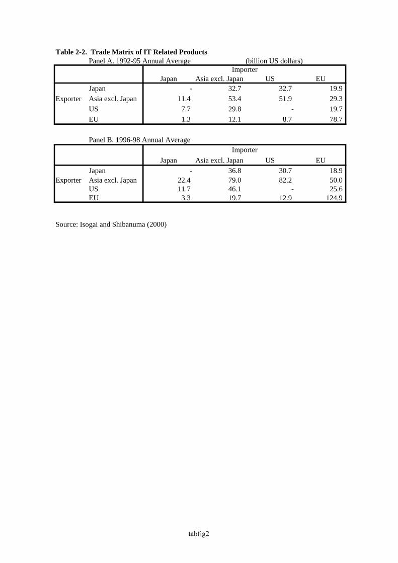
Table 2-2. Trade Matrix of IT Related ProductsPanel A. 1992-95 Annual Average (billion US dollars)

Japan Asia excl. Japan US EUJapan - 32.7 32.7 19.9

Exporter Asia excl. Japan 11.4 53.4 51.9 29.3US 7.7 29.8 - 19.7EU 1.3 12.1 8.7 78.7

Panel B. 1996-98 Annual Average

Japan Asia excl. Japan US EUJapan - 36.8 30.7 18.9

Exporter Asia excl. Japan 22.4 79.0 82.2 50.0US 11.7 46.1 - 25.6EU 3.3 19.7 12.9 124.9

Source: Isogai and Shibanuma (2000)

Importer

Importer

tabfig2

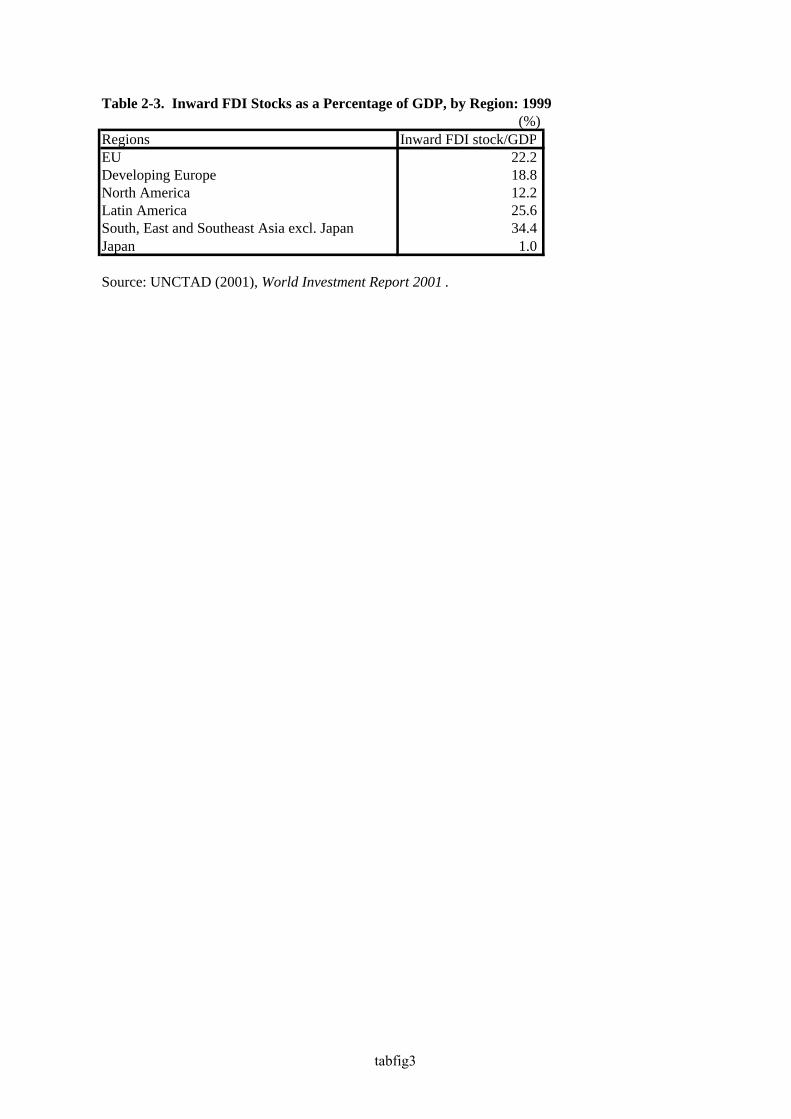
Table 2-3. Inward FDI Stocks as a Percentage of GDP, by Region: 1999(%)

Regions Inward FDI stock/GDPEU 22.2Developing Europe 18.8North America 12.2Latin America 25.6South, East and Southeast Asia excl. Japan 34.4Japan 1.0

Source: UNCTAD (2001), World Investment Report 2001 .

tabfig3

(%)

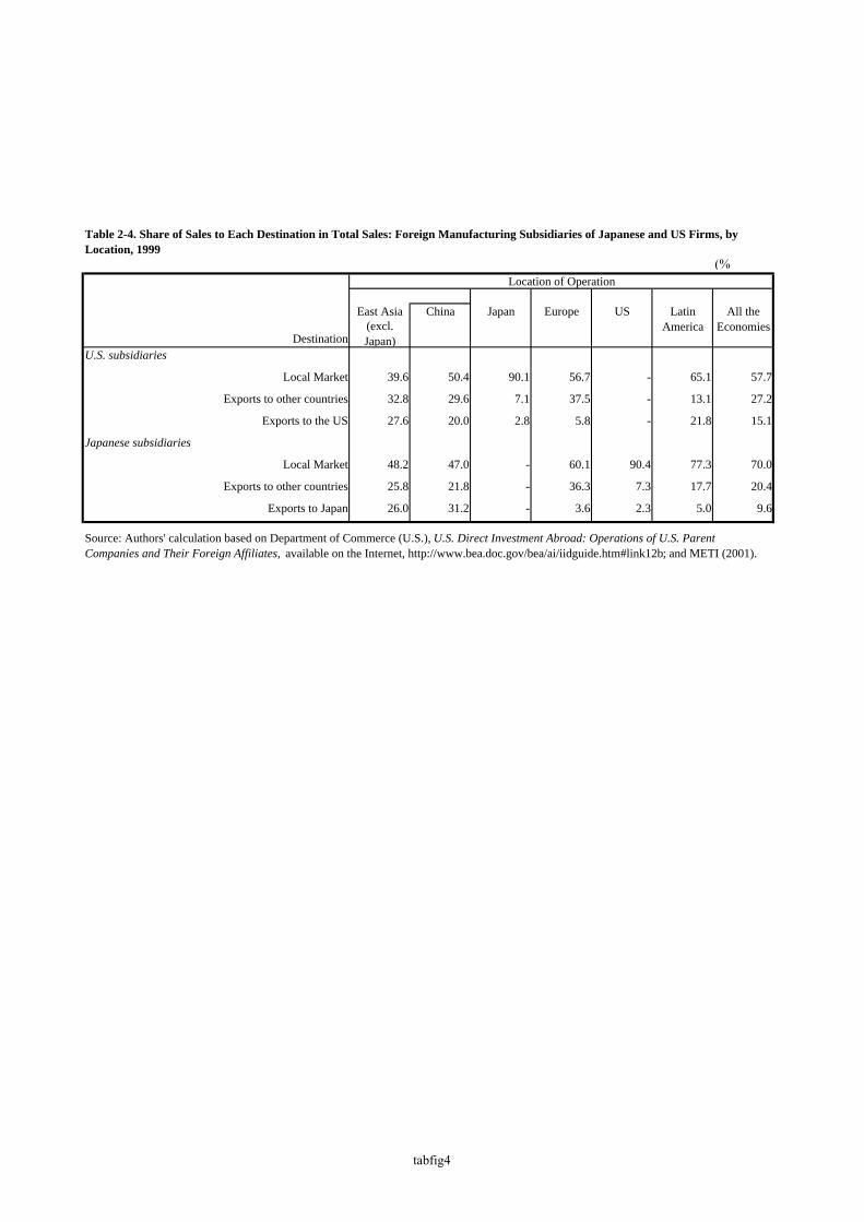
East Asia(excl.Japan)

U.S. subsidiaries

Local Market 39.6 50.4 90.1 56.7 - 65.1 57.7

Exports to other countries 32.8 29.6 7.1 37.5 - 13.1 27.2

Exports to the US 27.6 20.0 2.8 5.8 - 21.8 15.1

Japanese subsidiaries

Local Market 48.2 47.0 - 60.1 90.4 77.3 70.0

Exports to other countries 25.8 21.8 - 36.3 7.3 17.7 20.4

Exports to Japan 26.0 31.2 - 3.6 2.3 5.0 9.6

Source: Authors' calculation based on Department of Commerce (U.S.), U.S. Direct Investment Abroad: Operations of U.S. ParentCompanies and Their Foreign Affiliates, available on the Internet, http://www.bea.doc.gov/bea/ai/iidguide.htm#link12b; and METI (2001).

Table 2-4. Share of Sales to Each Destination in Total Sales: Foreign Manufacturing Subsidiaries of Japanese and US Firms, byLocation, 1999

Location of Operation

Destination

China Japan Europe US LatinAmerica

All theEconomies

tabfig4

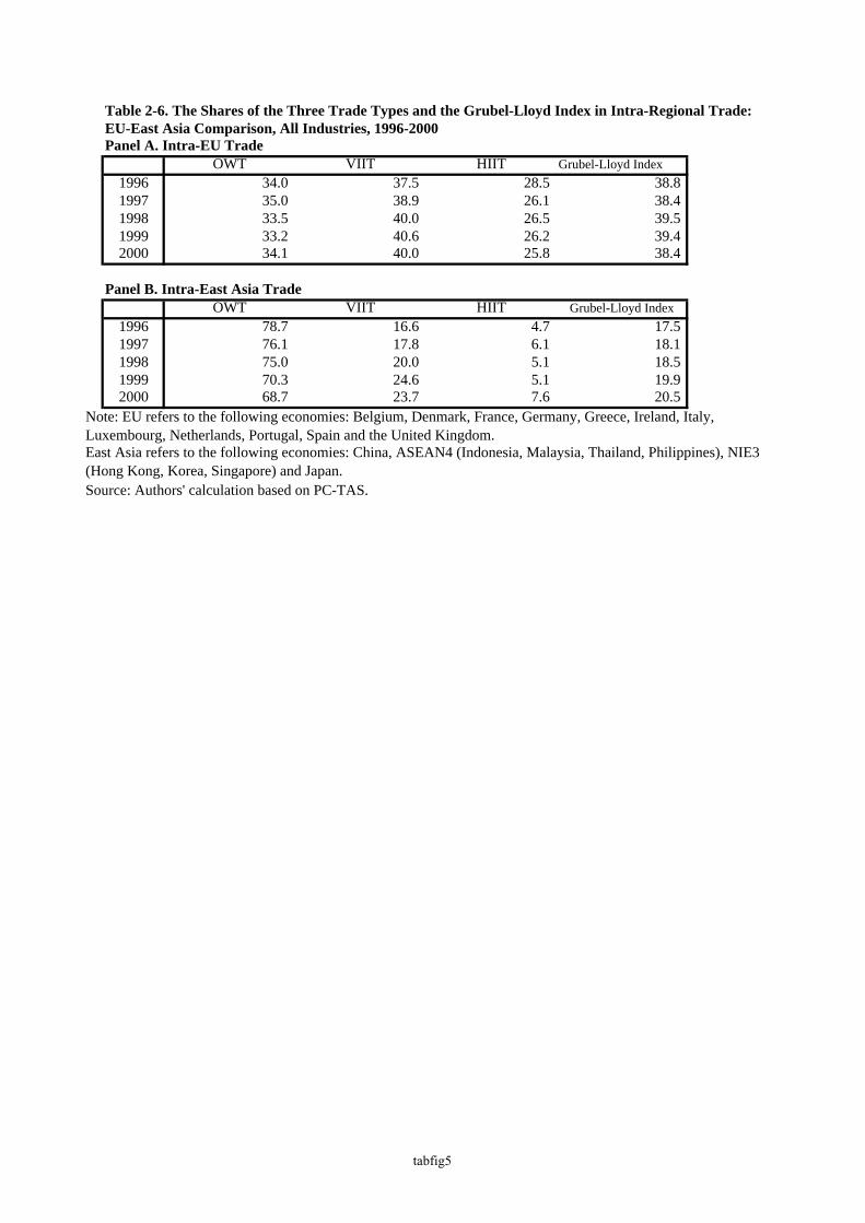
Table 2-6. The Shares of the Three Trade Types and the Grubel-Lloyd Index in Intra-Regional Trade: EU-East Asia Comparison, All Industries, 1996-2000Panel A. Intra-EU Trade

OWT VIIT HIIT Grubel-Lloyd Index1996 34.0 37.5 28.5 38.81997 35.0 38.9 26.1 38.41998 33.5 40.0 26.5 39.51999 33.2 40.6 26.2 39.42000 34.1 40.0 25.8 38.4

Panel B. Intra-East Asia TradeOWT VIIT HIIT Grubel-Lloyd Index

1996 78.7 16.6 4.7 17.51997 76.1 17.8 6.1 18.11998 75.0 20.0 5.1 18.51999 70.3 24.6 5.1 19.92000 68.7 23.7 7.6 20.5

Source: Authors' calculation based on PC-TAS.

Note: EU refers to the following economies: Belgium, Denmark, France, Germany, Greece, Ireland, Italy,Luxembourg, Netherlands, Portugal, Spain and the United Kingdom.East Asia refers to the following economies: China, ASEAN4 (Indonesia, Malaysia, Thailand, Philippines), NIE3(Hong Kong, Korea, Singapore) and Japan.

tabfig5

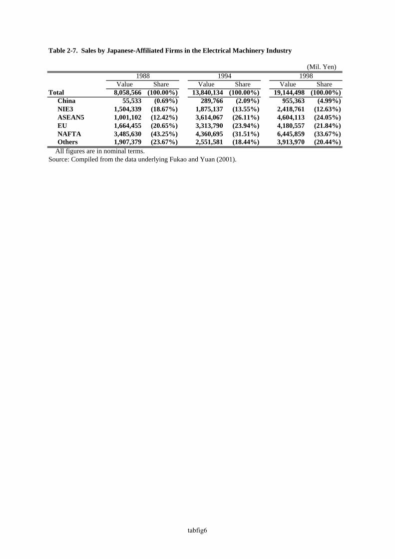
(Mil. Yen)

Value Share Value Share Value ShareTotal 8,058,566 (100.00%) 13,840,134 (100.00%) 19,144,498 (100.00%)

China 55,533 (0.69%) 289,766 (2.09%) 955,363 (4.99%)NIE3 1,504,339 (18.67%) 1,875,137 (13.55%) 2,418,761 (12.63%)ASEAN5 1,001,102 (12.42%) 3,614,067 (26.11%) 4,604,113 (24.05%)EU 1,664,455 (20.65%) 3,313,790 (23.94%) 4,180,557 (21.84%)NAFTA 3,485,630 (43.25%) 4,360,695 (31.51%) 6,445,859 (33.67%)Others 1,907,379 (23.67%) 2,551,581 (18.44%) 3,913,970 (20.44%)

All figures are in nominal terms.Source: Compiled from the data underlying Fukao and Yuan (2001).

1988 1994 1998

Table 2-7. Sales by Japanese-Affiliated Firms in the Electrical Machinery Industry

tabfig6

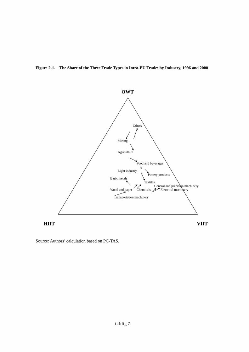
tabfig

7

Figure 2-1. The Share of the Three Trade Types in Intra-EU Trade: by Industry, 1996 and 2000

Source: Authors’ calculation based on PC-TAS.

Pottery products Basic metals

Transportation machinery

Others

Agriculture

Wood and paper

HIIT

OWT

VIIT

Food and beverages

Light industry

Mining

General and precision machinery Textiles

Electrical machinery Chemicals

tabfig

8

Figure 2-2. The Share of the Three Trade Types in Intra-East Asian Trade: by Industry, 1996

and 2000

Source: Authors’ calculation based on PC-TAS.

Pottery products Basic metals

Transportation machinery Others

Agriculture Wood and paper

HIIT

OWT

VIIT

Food and beverages

Light industry

Mining

General and precision machinery

Textiles

Electrical machinery

Chemicals

tabfig

9

Figure 2-3. The Share of the Three Trade Types in Intra-EU Trade: by Country, 1996 and 2000

Source: Authors’ calculation based on PC-TAS.

Greece

France Germany

Denmark

Italy

Ireland Portugal

HIIT

OWT

VIIT

Netherlands

Belgium& Luxembourg United Kingdom Spain

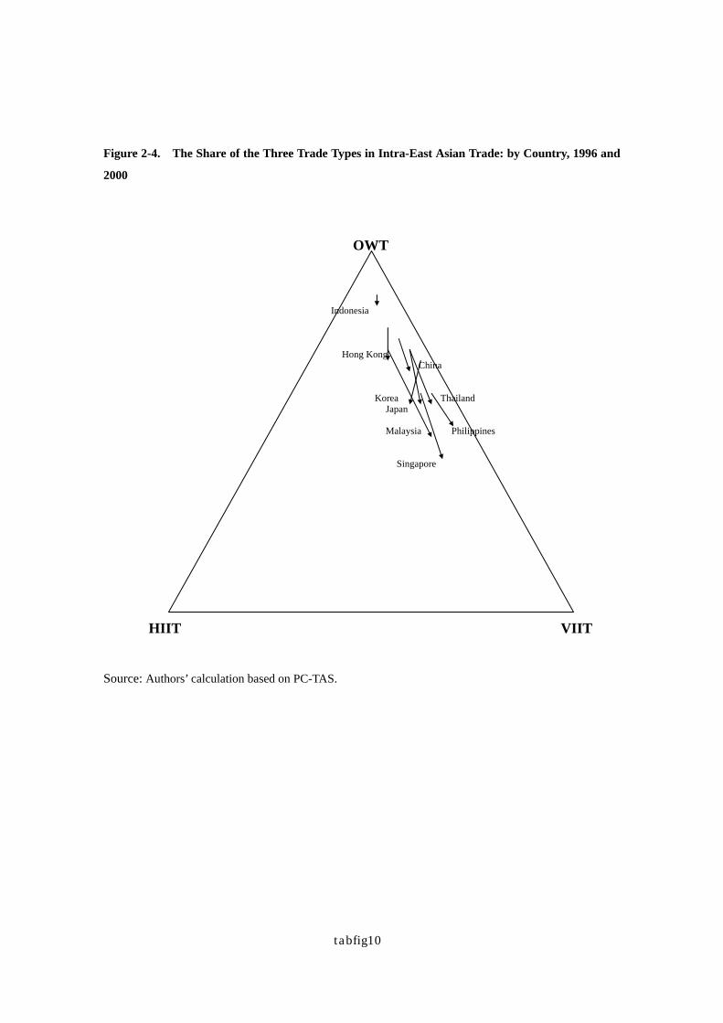
tabfig

10

Figure 2-4. The Share of the Three Trade Types in Intra-East Asian Trade: by Country, 1996 and

2000

Source: Authors’ calculation based on PC-TAS.

Malaysia Philippines

Thailand Japan

Korea

China Hong Kong

HIIT

OWT

VIIT

Singapore

Indonesia

tabfig

11

Figure 2-5. The Share of the Three Trade Types in Japan’s Bilateral Trade in Electrical Machinery: by Partner Region or Economy, 1988, 1994 and 2000

Note: The labels denote the following economies: Africa (Nigeria), ASEAN5 (Indonesia Malaysia,

Philippines, Singapore, Thailand), EU4 (France, Germany, Italy, UK), Middle East (Israel, Saudi Arabia), NAFTA (Canada, Mexico, USA), NIE3 (Hong Kong, Korea, Taiwan), Other Europe (Austria, Belgium, Denmark, Finland, Hungary, Ireland, Luxembourg, Netherlands, Norway, Poland, Portugal, Spain, Sweden, Switzerland), Pacific (Australia, New Zealand), Latin America (Argentina, Brazil, Columbia, Costa Rica, Panama, Peru, Venezuela).

Source: Authors’ calculation based on Japan’s trade statistics which are taken from http://www.customs.go.jp/toukei/download/index_d012_e.htm.

China

NIE3

ASEAN5

India Other Europe

EU4

Middle East

NAFTA

Latin America

Africa

Pacific

VIIT HIIT

OWT

tabfig

12

Figure 2-6. Share of Vertical Intra-Industry Trade in Japan's Trade with East Asian Countries:

--- Electrical Machinery Industry ---

(a) China and NIE3

0

10

20

30

40

50

60

70

1988 1989 1990 1991 1992 1993 1994 1995 1996 1997 1998 1999 2000

ChinaHong KongKoreaTaiwan

(%)

(b) ASEAN5

0

10

20

30

40

50

60

1988 1989 1990 1991 1992 1993 1994 1995 1996 1997 1998 1999 2000

IndonesiaMalaysiaPhilippinesSingaporeThailand

(%)

Note: Vertical IIT is identified using a 25% threshold as explained in Section 2. Source: Authors' calculation based on Japan's trade statistics taken from http://www.customs.go.jp/tokei/download/index_d012_e.htm.

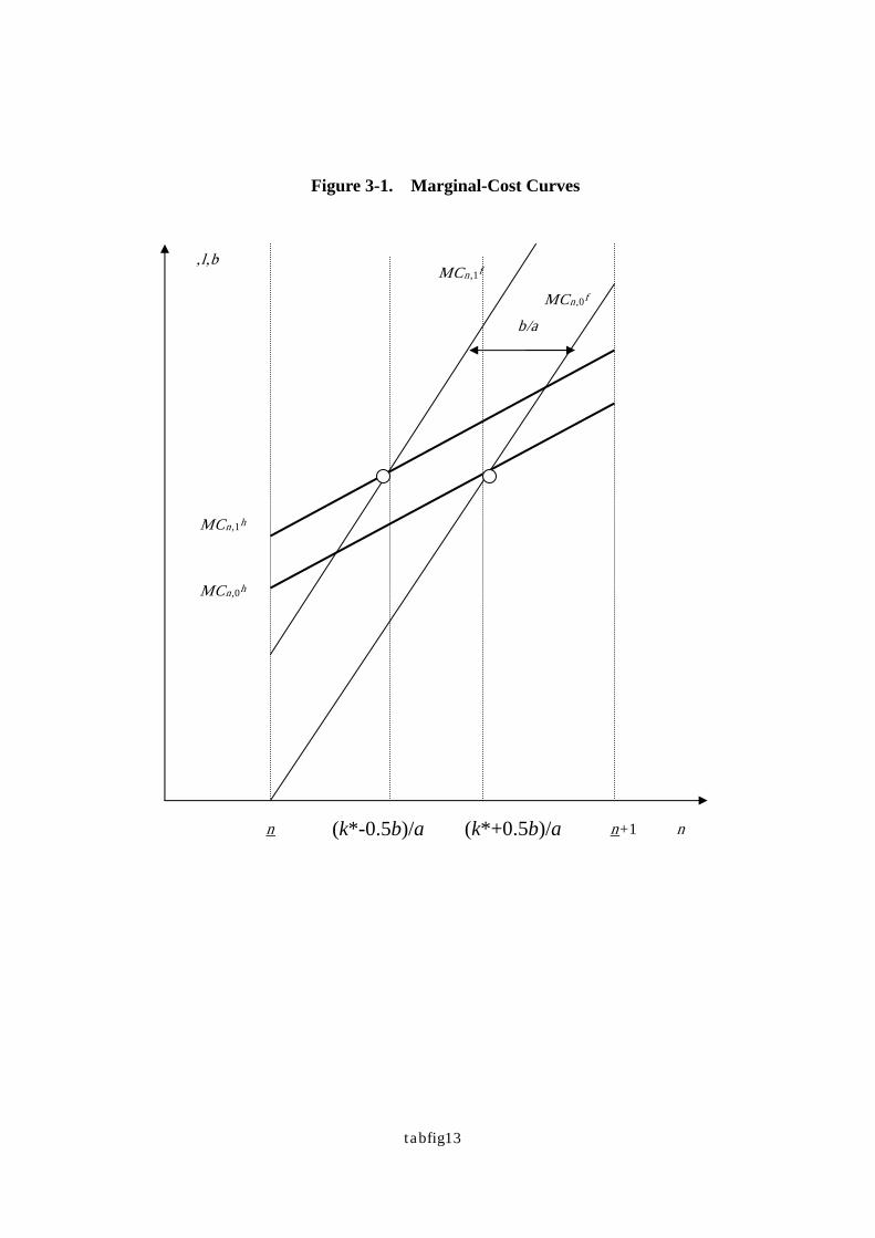
tabfig

13

Figure 3-1. Marginal-Cost Curves

n (k*-0.5b)/a (k*+0.5b)/a n+1

MCn,1f MCn,0f

MCn,0h

MCn,1h

b/a

n

‚l‚b

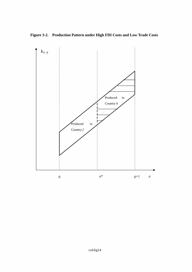
tabfig

14

Figure 3-2. Production Pattern under High FDI Costs and Low Trade Costs

n n* n+1 n

kn, q

Produced in

Country h

Produced in

Country f

tabfig

15

Figure 3-3. Production Pattern under Low FDI and Trade Costs

n n+1 n

kn, q

Produced in

Country h

Produced in

Country f

Produced in the

Two Countries

=VIIT

Produced in

Country h

k*

(k*+0.5b)/a (k*−0.5b)/a

b

d

g

h

a

e

f

c

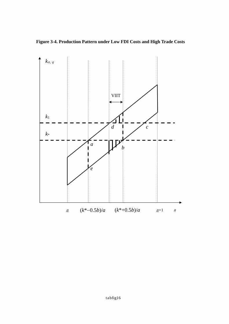
tabfig

16

Figure 3-4. Production Pattern under Low FDI Costs and High Trade Costs

n n+1 n

kn, q

VIIT

k*

(k*+0.5b)/a (k*−0.5b)/a

b

d

a

e

c

k1

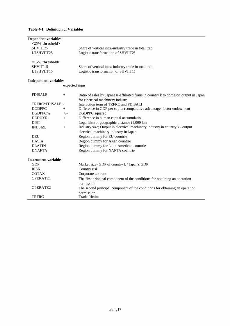
Table 4-1. Definition of Variables

Dependent variables<25% threshold>SHVIIT25 Share of vertical intra-industry trade in total tradeLTSHVIIT25 Logistic transformation of SHVIIT25

<15% threshold>SHVIIT15 Share of vertical intra-industry trade in total tradeLTSHVIIT15 Logistic transformation of SHVIIT15

Independent variablesexpected signs

FDISALE +

TRFRC*FDISALE - Interaction term of TRFRC and FDISALEDGDPPC + Difference in GDP per capita (comparative advantage, factor endowmentDGDPPC^2 +/- DGDPPC squaredDEDUYR + Difference in human capital accumulationDIST - Logarithm of geographic distance (1,000 km)INDSIZE +

DEU Region dummy for EU countriesDASIA Region dummy for Asian countrieDLATIN Region dummy for Latin American countrieDNAFTA Region dummy for NAFTA countrie

Instrument variablesGDP Market size (GDP of country k / Japan's GDP)RISK Country riskCOTAX Corporate tax rateOPERATE1

OPERATE2

TRFRC Trade friction

Ratio of sales by Japanese-affiliated firms in country k to domestic output in Japanfor electrical machinery industry

Industry size; Output in electrical machinery industry in country k / output electrical machinery industry in Japan

The first principal component of the conditions for obtaining an operationpermissionThe second principal component of the conditions for obtaining an operationpermission

tabfig17

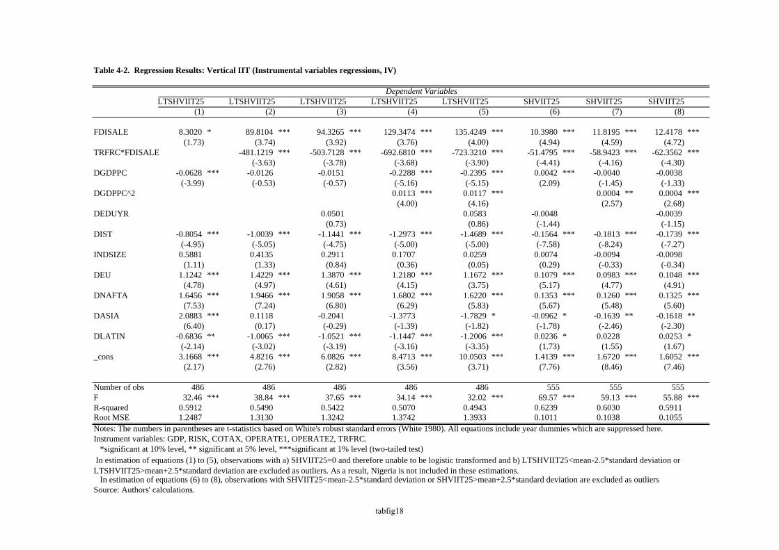
Table 4-2. Regression Results: Vertical IIT (Instrumental variables regressions, IV)

LTSHVIIT25 LTSHVIIT25 LTSHVIIT25 LTSHVIIT25 LTSHVIIT25 SHVIIT25 SHVIIT25 SHVIIT25(1) (2) (3) (4) (5) (6) (7) (8)

FDISALE 8.3020 * 89.8104 *** 94.3265 *** 129.3474 *** 135.4249 *** 10.3980 *** 11.8195 *** 12.4178 ***(1.73) (3.74) (3.92) (3.76) (4.00) (4.94) (4.59) (4.72)

TRFRC*FDISALE -481.1219 *** -503.7128 *** -692.6810 *** -723.3210 *** -51.4795 *** -58.9423 *** -62.3562 ***(-3.63) (-3.78) (-3.68) (-3.90) (-4.41) (-4.16) (-4.30)

DGDPPC -0.0628 *** -0.0126 -0.0151 -0.2288 *** -0.2395 *** 0.0042 *** -0.0040 -0.0038(-3.99) (-0.53) (-0.57) (-5.16) (-5.15) (2.09) (-1.45) (-1.33)

DGDPPC^2 0.0113 *** 0.0117 *** 0.0004 ** 0.0004 ***(4.00) (4.16) (2.57) (2.68)

DEDUYR 0.0501 0.0583 -0.0048 -0.0039(0.73) (0.86) (-1.44) (-1.15)

DIST -0.8054 *** -1.0039 *** -1.1441 *** -1.2973 *** -1.4689 *** -0.1564 *** -0.1813 *** -0.1739 ***(-4.95) (-5.05) (-4.75) (-5.00) (-5.00) (-7.58) (-8.24) (-7.27)

INDSIZE 0.5881 0.4135 0.2911 0.1707 0.0259 0.0074 -0.0094 -0.0098(1.11) (1.33) (0.84) (0.36) (0.05) (0.29) (-0.33) (-0.34)

DEU 1.1242 *** 1.4229 *** 1.3870 *** 1.2180 *** 1.1672 *** 0.1079 *** 0.0983 *** 0.1048 ***(4.78) (4.97) (4.61) (4.15) (3.75) (5.17) (4.77) (4.91)

DNAFTA 1.6456 *** 1.9466 *** 1.9058 *** 1.6802 *** 1.6220 *** 0.1353 *** 0.1260 *** 0.1325 ***(7.53) (7.24) (6.80) (6.29) (5.83) (5.67) (5.48) (5.60)

DASIA 2.0883 *** 0.1118 -0.2041 -1.3773 -1.7829 * -0.0962 * -0.1639 ** -0.1618 **(6.40) (0.17) (-0.29) (-1.39) (-1.82) (-1.78) (-2.46) (-2.30)

DLATIN -0.6836 ** -1.0065 *** -1.0521 *** -1.1447 *** -1.2006 *** 0.0236 * 0.0228 0.0253 *(-2.14) (-3.02) (-3.19) (-3.16) (-3.35) (1.73) (1.55) (1.67)

_cons 3.1668 *** 4.8216 *** 6.0826 *** 8.4713 *** 10.0503 *** 1.4139 *** 1.6720 *** 1.6052 ***(2.17) (2.76) (2.82) (3.56) (3.71) (7.76) (8.46) (7.46)

Number of obs 486 486 486 486 486 555 555 555F 32.46 *** 38.84 *** 37.65 *** 34.14 *** 32.02 *** 69.57 *** 59.13 *** 55.88 ***R-squared 0.5912 0.5490 0.5422 0.5070 0.4943 0.6239 0.6030 0.5911Root MSE 1.2487 1.3130 1.3242 1.3742 1.3933 0.1011 0.1038 0.1055Notes: The numbers in parentheses are t-statistics based on White's robust standard errors (White 1980). All equations include year dummies which are suppressed here.Instrument variables: GDP, RISK, COTAX, OPERATE1, OPERATE2, TRFRC. *significant at 10% level, ** significant at 5% level, ***significant at 1% level (two-tailed test)

In estimation of equations (6) to (8), observations with SHVIIT25<mean-2.5*standard deviation or SHVIIT25>mean+2.5*standard deviation are excluded as outliersSource: Authors' calculations.

Dependent Variables

In estimation of equations (1) to (5), observations with a) SHVIIT25=0 and therefore unable to be logistic transformed and b) LTSHVIIT25<mean-2.5*standard deviation orLTSHVIIT25>mean+2.5*standard deviation are excluded as outliers. As a result, Nigeria is not included in these estimations.

tabfig18

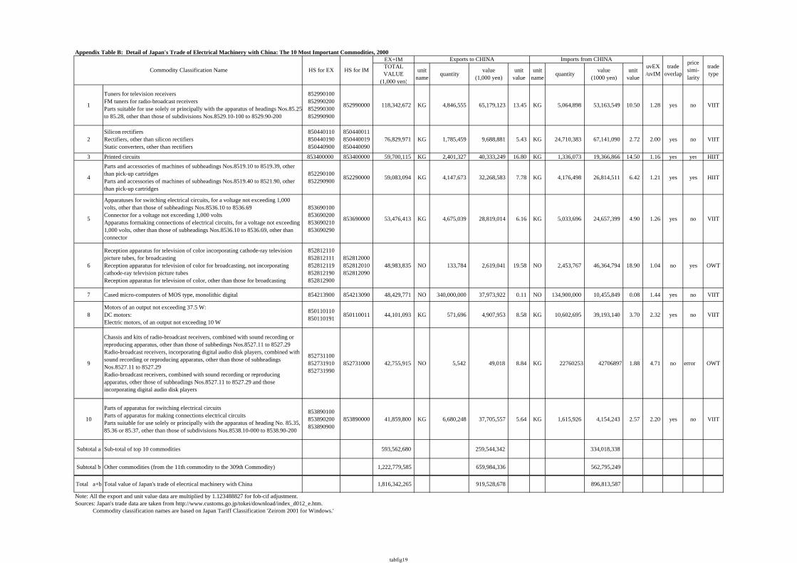
Appendix Table B: Detail of Japan's Trade of Electrical Machinery with China: The 10 Most Important Commodities, 2000EX+IMTOTALVALUE

(1,000 yen)

unitname quantity value

(1,000 yen)unit

valueunit

name quantity value(1000 yen)

unitvalue

1

Tuners for television receiversFM tuners for radio-broadcast receiversParts suitable for use solely or principally with the apparatus of headings Nos.85.25to 85.28, other than those of subdivisions Nos.8529.10-100 to 8529.90-200

852990100852990200852990300852990900

852990000 118,342,672 KG 4,846,555 65,179,123 13.45 KG 5,064,898 53,163,549 10.50 1.28 yes no VIIT

2Silicon rectifiersRectifiers, other than silicon rectifiersStatic converters, other than rectifiers

850440110850440190850440900

850440011850440019850440090

76,829,971 KG 1,785,459 9,688,881 5.43 KG 24,710,383 67,141,090 2.72 2.00 yes no VIIT

3 Printed circuits 853400000 853400000 59,700,115 KG 2,401,327 40,333,249 16.80 KG 1,336,073 19,366,866 14.50 1.16 yes yes HIIT

4

Parts and accessories of machines of subheadings Nos.8519.10 to 8519.39, otherthan pick-up cartridgesParts and accessories of machines of subheadings Nos.8519.40 to 8521.90, otherthan pick-up cartridges

852290100852290900 852290000 59,083,094 KG 4,147,673 32,268,583 7.78 KG 4,176,498 26,814,511 6.42 1.21 yes yes HIIT

5

Apparatuses for switching electrical circuits, for a voltage not exceeding 1,000volts, other than those of subheadings Nos.8536.10 to 8536.69Connector for a voltage not exceeding 1,000 voltsApparatus formaking connections of electrical circuits, for a voltage not exceeding1,000 volts, other than those of subheadings Nos.8536.10 to 8536.69, other thanconnector

853690100853690200853690210853690290

853690000 53,476,413 KG 4,675,039 28,819,014 6.16 KG 5,033,696 24,657,399 4.90 1.26 yes no VIIT

6

Reception apparatus for television of color incorporating cathode-ray televisionpicture tubes, for broadcastingReception apparatus for television of color for broadcasting, not incorporatingcathode-ray television picture tubesReception apparatus for television of color, other than those for broadcasting

852812110852812111852812119852812190852812900

852812000852812010852812090

48,983,835 NO 133,784 2,619,041 19.58 NO 2,453,767 46,364,794 18.90 1.04 no yes OWT

7 Cased micro-computers of MOS type, monolithic digital 854213900 854213090 48,429,771 NO 340,000,000 37,973,922 0.11 NO 134,900,000 10,455,849 0.08 1.44 yes no VIIT

8Motors of an output not exceeding 37.5 W:DC motors:Electric motors, of an output not exceeding 10 W

850110110850110191 850110011 44,101,093 KG 571,696 4,907,953 8.58 KG 10,602,695 39,193,140 3.70 2.32 yes no VIIT

9

Chassis and kits of radio-broadcast receivers, combined with sound recording orreproducing apparatus, other than those of subhedings Nos.8527.11 to 8527.29Radio-broadcast receivers, incorporating digital audio disk players, combined withsound recording or reproducing apparatus, other than those of subheadingsNos.8527.11 to 8527.29Radio-broadcast receivers, combined with sound recording or reproducingapparatus, other those of subheadings Nos.8527.11 to 8527.29 and thoseincorporating digital audio disk players

852731100852731910852731990

852731000 42,755,915 NO 5,542 49,018 8.84 KG 22760253 42706897 1.88 4.71 no error OWT

10

Parts of apparatus for switching electrical circuitsParts of apparatus for making connections electrical circuitsParts suitable for use solely or principally with the apparatus of heading No. 85.35,85.36 or 85.37, other than those of subdivisions Nos.8538.10-000 to 8538.90-200

853890100853890200853890900

853890000 41,859,800 KG 6,680,248 37,705,557 5.64 KG 1,615,926 4,154,243 2.57 2.20 yes no VIIT

Subtotal a Sub-total of top 10 commodities 593,562,680 259,544,342 334,018,338

Subtotal b Other commodities (from the 11th commodity to the 309th Commodity) 1,222,779,585 659,984,336 562,795,249

Total a+b Total value of Japan's trade of elecrtical machinery with China 1,816,342,265 919,528,678 896,813,587

Note: All the export and unit value data are multiplied by 1.123488827 for fob-cif adjustment.Sources: Japan's trade data are taken from http://www.customs.go.jp/tokei/download/index_d012_e.htm. Commodity classification names are based on Japan Tariff Classification 'Zeirom 2001 for Windows.'

Commodity Classification Name HS for EX HS for IM

Exports to CHINAtradetype

Imports from CHINAuvEX/uvIM

tradeoverlap

pricesimi-larity

tabfig19

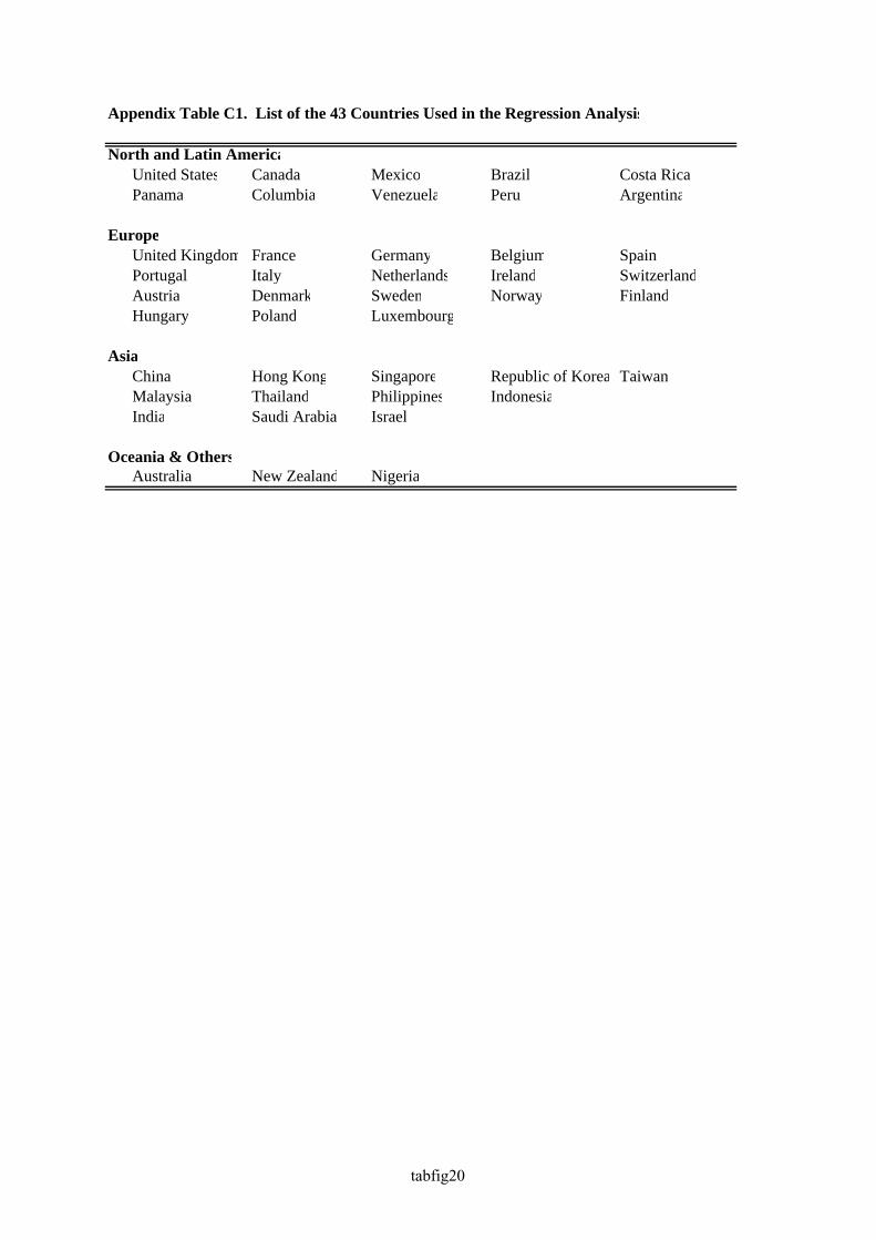
Appendix Table C1. List of the 43 Countries Used in the Regression Analysis

North and Latin AmericaUnited States Canada Mexico Brazil Costa RicaPanama Columbia Venezuela Peru Argentina

EuropeUnited Kingdom France Germany Belgium SpainPortugal Italy Netherlands Ireland SwitzerlandAustria Denmark Sweden Norway FinlandHungary Poland Luxembourg

AsiaChina Hong Kong Singapore Republic of Korea TaiwanMalaysia Thailand Philippines IndonesiaIndia Saudi Arabia Israel

Oceania & OthersAustralia New Zealand Nigeria

tabfig20

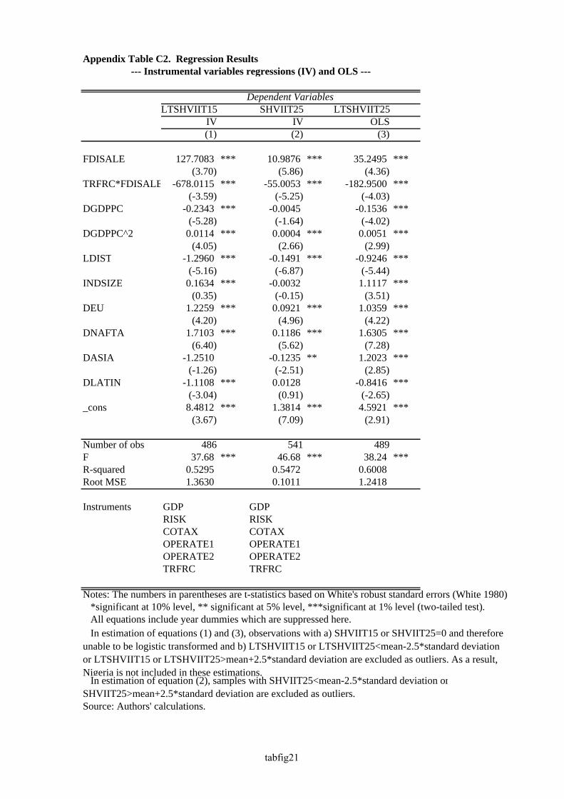
Appendix Table C2. Regression Results

LTSHVIIT15 SHVIIT25 LTSHVIIT25IV IV OLS(1) (2) (3)

FDISALE 127.7083 *** 10.9876 *** 35.2495 ***(3.70) (5.86) (4.36)

TRFRC*FDISALE -678.0115 *** -55.0053 *** -182.9500 ***(-3.59) (-5.25) (-4.03)

DGDPPC -0.2343 *** -0.0045 -0.1536 ***(-5.28) (-1.64) (-4.02)

DGDPPC^2 0.0114 *** 0.0004 *** 0.0051 ***(4.05) (2.66) (2.99)

LDIST -1.2960 *** -0.1491 *** -0.9246 ***(-5.16) (-6.87) (-5.44)

INDSIZE 0.1634 *** -0.0032 1.1117 ***(0.35) (-0.15) (3.51)

DEU 1.2259 *** 0.0921 *** 1.0359 ***(4.20) (4.96) (4.22)

DNAFTA 1.7103 *** 0.1186 *** 1.6305 ***(6.40) (5.62) (7.28)

DASIA -1.2510 -0.1235 ** 1.2023 ***(-1.26) (-2.51) (2.85)

DLATIN -1.1108 *** 0.0128 -0.8416 ***(-3.04) (0.91) (-2.65)

_cons 8.4812 *** 1.3814 *** 4.5921 ***(3.67) (7.09) (2.91)

Number of obs 486 541 489F 37.68 *** 46.68 *** 38.24 ***R-squared 0.5295 0.5472 0.6008Root MSE 1.3630 0.1011 1.2418

Instruments GDP GDPRISK RISKCOTAX COTAXOPERATE1 OPERATE1OPERATE2 OPERATE2TRFRC TRFRC

Notes: The numbers in parentheses are t-statistics based on White's robust standard errors (White 1980) *significant at 10% level, ** significant at 5% level, ***significant at 1% level (two-tailed test). All equations include year dummies which are suppressed here.

Source: Authors' calculations.

In estimation of equation (2), samples with SHVIIT25<mean-2.5*standard deviation orSHVIIT25>mean+2.5*standard deviation are excluded as outliers.

Dependent Variables

--- Instrumental variables regressions (IV) and OLS ---

In estimation of equations (1) and (3), observations with a) SHVIIT15 or SHVIIT25=0 and thereforeunable to be logistic transformed and b) LTSHVIIT15 or LTSHVIIT25<mean-2.5*standard deviationor LTSHVIIT15 or LTSHVIIT25>mean+2.5*standard deviation are excluded as outliers. As a result,Nigeria is not included in these estimations.

tabfig21

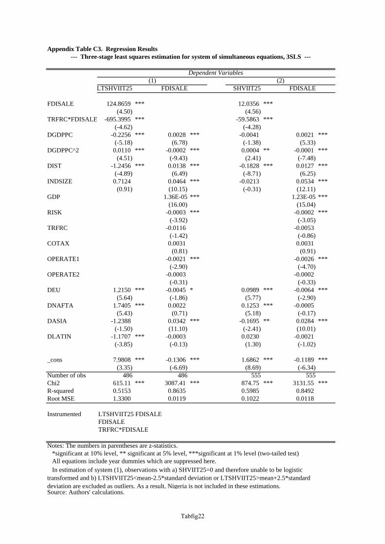
Appendix Table C3. Regression Results

LTSHVIIT25 FDISALE SHVIIT25 FDISALE

FDISALE 124.8659 *** 12.0356 ***(4.50) (4.56)

TRFRC*FDISALE -695.3995 *** -59.5863 ***(-4.62) (-4.28)

DGDPPC -0.2256 *** 0.0028 *** -0.0041 0.0021 ***(-5.18) (6.78) (-1.38) (5.33)

DGDPPC^2 0.0110 *** -0.0002 *** 0.0004 ** -0.0001 ***(4.51) (-9.43) (2.41) (-7.48)

DIST -1.2456 *** 0.0138 *** -0.1828 *** 0.0127 ***(-4.89) (6.49) (-8.71) (6.25)

INDSIZE 0.7124 0.0464 *** -0.0213 0.0534 ***(0.91) (10.15) (-0.31) (12.11)

GDP 1.36E-05 *** 1.23E-05 ***(16.00) (15.04)

RISK -0.0003 *** -0.0002 ***(-3.92) (-3.05)

TRFRC -0.0116 -0.0053(-1.42) (-0.86)

COTAX 0.0031 0.0031(0.81) (0.91)

OPERATE1 -0.0021 *** -0.0026 ***(-2.90) (-4.70)

OPERATE2 -0.0003 -0.0002(-0.31) (-0.33)

DEU 1.2150 *** -0.0045 * 0.0989 *** -0.0064 ***(5.64) (-1.86) (5.77) (-2.90)

DNAFTA 1.7405 *** 0.0022 0.1253 *** -0.0005(5.43) (0.71) (5.18) (-0.17)

DASIA -1.2388 0.0342 *** -0.1695 ** 0.0284 ***(-1.50) (11.10) (-2.41) (10.01)

DLATIN -1.1707 *** -0.0003 0.0230 -0.0021(-3.85) (-0.13) (1.30) (-1.02)

_cons 7.9808 *** -0.1306 *** 1.6862 *** -0.1189 ***(3.35) (-6.69) (8.69) (-6.34)

Number of obs 486 486 555 555Chi2 615.11 *** 3087.41 *** 874.75 *** 3131.55 ***R-squared 0.5153 0.8635 0.5985 0.8492Root MSE 1.3300 0.0119 0.1022 0.0118

Instrumented LTSHVIIT25 FDISALEFDISALETRFRC*FDISALE

Notes: The numbers in parentheses are z-statistics. *significant at 10% level, ** significant at 5% level, ***significant at 1% level (two-tailed test). All equations include year dummies which are suppressed here.

Source: Authors' calculations.

In estimation of system (1), observations with a) SHVIIT25=0 and therefore unable to be logistictransformed and b) LTSHVIIT25<mean-2.5*standard deviation or LTSHVIIT25>mean+2.5*standarddeviation are excluded as outliers. As a result, Nigeria is not included in these estimations.

--- Three-stage least squares estimation for system of simultaneous equations, 3SLS ---

Dependent Variables(1) (2)

Tabfig22