Embed Size (px)
Citation preview
UNCLASSIFIED QinetiQ Proprietary
Copyright © QinetiQ ltd 2008 QinetiQ Proprietary UNCLASSIFIED
Vertical Axis Wind Turbine Radar Impact Assessment
Chris New, Sebastian Di Laura QINETIQ/IS/ICS/TR0800446/1.0 July 2008
UNCLASSIFIED QinetiQ Proprietary
QINETIQ/IS/ICS/TR0800446/1.0 Page 2 of 82 QinetiQ Proprietary
UNCLASSIFIED
Administration page Customer Information
Customer reference number
Project title Vertical Axis Wind Turbine – Radar Impact Assessment
Customer Organisation Air Defence and Air Traffic Services Integrated Project Team
Customer contact Group Captain Maurice Dixon
Contract number FTS2/025
Milestone number 3
Date due 30 June 2008
Principal authors
Chris New 02392 312159
Block 3, Room 8, Portsdown Technology Park, Southwick Road, Cosham, PO6 3RU
Sebastian Di Laura 02392 312233
Block 3, Room 16, Portsdown Technology Park, Southwick Road, Cosham, PO6 3RU
Release Authority
Name Samantha Dearman
Post Project Manager
Date of issue 1 July 2008
Record of changes
Issue Date Detail of Changes
0.1 30 April 2008 First draft
1.0 1st July 2008 First issue
UNCLASSIFIED QinetiQ Proprietary
QINETIQ/IS/ICS/TR0800446/1.0 Page 3 of 82 QinetiQ Proprietary
UNCLASSIFIED
Executive summary QinetiQ was contracted by the Air Defence and Air Traffic Services Integrated Project Team to predict and measure the radar cross section (RCS) of a vertical axis wind turbine (VAWT), as well as assess the potential impact it would have on radar. The VAWT used for the study was the Quiet Revolution (QR) qr5, a 7kW turbine that is roughly 5 metres high and 3 metres in width.
To predict the RCS of the VAWT, a computer aided design (CAD) model was created, with a finite element mesh applied to it. The RCS predictions were calculated using the QinetiQ RCS prediction tool, Spectre®. The configuration tool was set up to run at frequencies of 1.3GHz and 2.9GHz, to represent L-Band and S-Band radars, at elevation angles of 0 and 1 degrees for a perfect electric conductor (PEC) material turbine assembly in free space.
The analysis showed that the dominant source of RCS was the central vertical axis of the VAWT, with a peak RCS of 20.5dBsm depending on the frequency and elevation angle, which masked some of the reflections from the blades. The RCS predictions were repeated with a radar absorbent material (RAM) applied to the vertical axis, which reduced the peak RCS to 11.5dBsm.
A spectrogram analysis was carried out, allowing Doppler velocity information to be extracted from the RCS data. Identifying the RCS of the moving components is important since many types of radar in the United Kingdom use filters to remove signals from static, or slow moving, objects. Therefore, it is the RCS from the moving parts of the turbine, with speeds roughly greater than 10 metres per second, that is likely to have the greatest impact on radar. The peak RCS from a moving component was predicted to be of the order of 4.8dBsm.
A real radar measurement trial was also undertaken by installing a QR qr5 VAWT at the QinetiQ Funtington measurement range on the south coast of England. The final set up of the turbine meant that the radar elevation angle with respect to the turbine was 1.6 degrees, slightly more than was originally modelled with Spectre. Measurements were taken at both 1.3GHz and 2.9GHz using vertical and horizontal polarisations. The peak RCS measured was found to be 18.8dBsm, with a peak RCS from a moving component of 1.1dBsm.
Comparing the measured data to that of the modelled data showed some good agreement when using the 1 degree elevation RAM axis data set. It was decided to run additional Spectre modelling to assess the RCS of the VAWT at 1.6 degrees. Comparing these additional results yielded better agreement between the modelled and measured data sets. It was found that the RCS of the VAWT was extremely sensitive to elevation angle, particularly at 2.9GHz. At 1.6 degrees elevation angle there appeared to be minimal reflection from the vertical axis of the VAWT, which was the dominant feature at 0 and 1 degrees, and explains why the RAM modelled data compared better against the real data than the PEC modelling.
Further analysis showed that overall, the measured data seemed to be slightly higher in RCS than the modelled data, but the high level of background noise in the real measurements made it difficult to pick out some of the blade structure in the Doppler spectra. When comparing images of the real VAWT installed at Funtington to that of the CAD used in the modelling, differences were found which were likely to account for the variations in the data.
UNCLASSIFIED QinetiQ Proprietary
QINETIQ/IS/ICS/TR0800446/1.0 Page 4 of 82 QinetiQ Proprietary
UNCLASSIFIED
The last part of this study examined the detection ranges and cumulative effects for a VAWT. At certain elevation angles, the radar has the potential to see the static component of the turbine out to a range of 32-138km. However, these detection ranges have been calculated in a free space environment without terrain clutter or multipath effects. The static clutter created by the VAWT would be set amongst other real world objects such as houses or lampposts, typical of an urban area
At certain elevation angles, the radar has the potential to see the moving component of the turbine out to a range of approximately 51km. Again, urban clutter attributed to cars and trucks, which have a comparable RCS return, would have already created similar clutter levels. Therefore, the addition of a VAWT to this clutter would have limited impact.
Taking into account the use of moving target indicator (MTI) filters in radar, and the likely clutter levels and obscuration associated with the urban environment, it is highly unlikely that a VAWT will add any additional clutter levels to that already seen and dealt with by a radar.
UNCLASSIFIED QinetiQ Proprietary
QINETIQ/IS/ICS/TR0800446/1.0 Page 5 of 82 QinetiQ Proprietary
UNCLASSIFIED
List of contents 1 Introduction 7
1.1 Contractual 7 1.2 Background 7 1.2.1 Impact of turbines on aviation 7 1.2.2 Vertical axis wind turbines 8 1.3 Structure of the report 8
2 Computer Aided Design Modelling and Analysis 9 2.1 Methods of analysis 9 2.1.1 Spectre 9 2.1.2 Computer aided design and mesh 10 2.1.3 Computer aided design model of the Quiet Revolution vertical axis
wind turbine 10 2.1.4 General settings and assumptions 12 2.2 Modelling results 13 2.2.1 Radar cross section results for the vertical axis wind turbine at 0
degree elevation 13 2.2.2 Radar cross section results for the vertical axis wind turbine at 1
degree elevation 22 2.2.3 Radar cross section comparison with the vertical axis covered with
perfect radar absorbent material 24 2.2.4 Summary of Spectre radar cross section modelling 30
3 Vertical Axis Wind Turbine Measurements and Analysis 33 3.1 Installation and set up 33 3.2 L-Band measurements 36 3.2.1 120 revolutions per minute 36 3.2.2 60 revolutions per minute 37 3.3 S-Band measurements 38 3.3.1 120 revolutions per minute 38 3.3.2 60 revolutions per minute 39 3.4 Summary 40 3.5 Modelled versus measurement 41
4 Assessment of the Impact of a Vertical Axis Wind Turbine 53 4.1 Comparison with other targets 53 4.2 Minimum detectable radar cross section 54 4.3 Range a vertical axis wind turbine become visible 55 4.4 Cumulative effect on detection range 57 4.5 Impact summary 60

UNCLASSIFIED QinetiQ Proprietary
QINETIQ/IS/ICS/TR0800446/1.0 Page 6 of 82 QinetiQ Proprietary
UNCLASSIFIED
5 Conclusions 61
6 References 63
7 Abbreviations 64
A Appendix A – Radar Cross Section Plots and Hotspots/Energy Path Displays 65 A.1 Radar cross section plots for turbine assembly 65 A.2 Hotspot and energy path displays for 1.3GHz 69 A.3 Hotspot and energy path displays for 2.9GHz 75
UNCLASSIFIED QinetiQ Proprietary
QINETIQ/IS/ICS/TR0800446/1.0 Page 7 of 82 QinetiQ Proprietary
UNCLASSIFIED
1 Introduction
1.1 Contractual
This report has been prepared by QinetiQ for the Air Defence and Air Traffic Services (ADATS) Integrated Project Team (IPT) under contract number FTS2/025.
The scope of the study was to predict the radar cross section (RCS) of the Quiet Revolution (QR) qr5 vertical axis wind turbine (VAWT) [1] at 1.3GHz and 2.9GHz, equating to L-Band and S-Band radar frequencies, and compared the results to real measurements undertaken at the QinetiQ Funtington measurement range on the south coast of England. The final part of the study assessed the potential impact the VAWT may have on radar.
1.2 Background
1.2.1 Impact of turbines on aviation
Wind power is considered to be a major contributor to the Government’s 2010 target of generating 10% of all electricity from renewable sources [1]. However, wind power does not come without complications, predominantly due to the physical structures of the wind turbines on the landscape. Wind turbines also have the potential to interfere with aviation operations, in terms of physical obstructions and also with the radars that survey and monitor the air traffic environment. The potential aviation impact from wind turbines is generally greater as the number of turbines, and their height above ground level, increase.
Wind farms, in common with any large manmade structure, are a potential source of clutter1 with a large static RCS and can create areas of clutter on a radar display screen. This clutter can be removed by using moving target indicator (MTI2) filters. However, the rotation of the blades also causes intermittent clutter in the MTI output of the radar; leading to the possibility of track-like plots in the region of the wind farm, which is the main source of the impact of wind farms on radar systems. Busy roads and wind blown rain are other common sources of MTI clutter for radar systems.
If the region affected by the wind farm is large enough, even known aircraft can be more difficult to differentiate as they fly over the turbines, and detection of the aircraft may be lost. All of this greatly decreases the ability of the air traffic controller (ATCO) to do an effective job, and maintain a safe operating environment.
Both wind energy and aviation are important to United Kingdom (UK) national interests and both industry sectors have legitimate interests that need to be balanced. In order to strike this balance it is important that the wind energy and aviation communities understand their respective needs.
1 Clutter is a radar term for unwanted returns such as radar reflections from buildings, rain, or hills. 2 MTI uses the familiar Doppler Effect, which causes a shift in frequency due to an object’s motion towards, or away from, the radar to discriminate moving targets from stationary clutter.
UNCLASSIFIED QinetiQ Proprietary
QINETIQ/IS/ICS/TR0800446/1.0 Page 8 of 82 QinetiQ Proprietary
UNCLASSIFIED
1.2.2 Vertical axis wind turbines
As part of the renewable energy culture that exists today, a new design of wind turbine has manifested itself into the market place, specifically intended for the turbulent urban environment. Their primary purpose is for installation on the roofs of buildings rather than in remote fields in large wind farms. Therefore, VAWTs are designed to have a relatively small spatial footprint, whilst being as efficient as possible without necessarily having a continuous source of clean flowing wind.
As the UK population is urged to reduce their carbon footprint, VAWTs are becoming more popular, especially as many of them are aesthetically pleasing, and are gaining favour with architects.
At present, planning application processes for large, more conventional wind turbines, are thorough and stringent due to the many different impacts that the turbines can have for the environment and aviation. However, due to their small size, planning processes for small scale wind turbines are much less stringent [1].
Little is known about the impact of VAWTs on radar and with the relaxed planning requirements there is the possibility whereby a number of buildings could have a significant number of them installed, without having to consult with the aviation stakeholders.
The aim of this report is to increase the understanding of the impact of a VAWT on radar, and quantify the magnitude of this impact. With RCS being frequency dependent, the study is being undertaken at two frequencies, 1.3GHz and 2.9GHz, which are the main frequencies used in the UK for air defence and air traffic control radars.
1.3 Structure of the report
The structure of the report is as follows: • Section 2: Computer Aided Design Modelling and Analysis
• Section 3: Vertical Axis Wind Turbine Measurements and Analysis
• Section 4: Assessment of the Impact of a Vertical Axis Wind Turbine
• Section 5: Conclusions
• Section 6: References
• Section 7: Abbreviations
UNCLASSIFIED QinetiQ Proprietary
QINETIQ/IS/ICS/TR0800446/1.0 Page 9 of 82 QinetiQ Proprietary
UNCLASSIFIED
2 Computer Aided Design Modelling and Analysis This section provides an overview of the modelling process, discusses the QinetiQ RCS prediction code, Spectre®, the computer aided design (CAD) input for the turbine design, the parameters for the explicit calculations and, finally, the general assumptions used to obtain the RCS predictions.
2.1 Methods of analysis
2.1.1 Spectre
Spectre is an RCS prediction code, developed by QinetiQ to model the RCS of large, complex objects. Development began in the mid-1980s and the code has been operational since 1990, having been thoroughly validated against measured data. The tool provides guidance on the radar signatures of complex objects and is subject to continuous development to enhance its capabilities and computing efficiency. The program has been validated against a variety of shapes, including basic geometric objects, scale models and full-scale ships at sea.
Spectre can deal with reflections from perfectly conducting and dielectric coated surfaces, as well as edge diffraction.
A typical Spectre modelling process commences with the use of a computer aided engineering (CAE) package used to import a CAD provided by an external source. The CAE package is used to cover the surface of the CAD model with a series of flat triangular and quadrilateral elements, known as a finite element mesh (FEM). It is this mesh that Spectre uses for the RCS calculations.
Spectre can only produce reasonable answers if the FEM it uses is a reasonable description of the target it corresponds to. Although it can be tempting to use a geometrical description that looks acceptable to the naked eye, this can lead to significant errors in practice.
The FEM must be an accurate representation of the object that is being simulated. In a strict sense, this means that it should be within 1/16 of a wavelength (approximately 6mm in this analysis) of the true geometry at all points, but for many cases this is impossible to achieve as objects often change shape slightly due to the forces of motion or changes in the environment.
Although not universal rules, the following provide an idea of the sensitivity of the results to the input FEM:
• RCS is relatively insensitive to small changes in curved objects, but sensitive to small changes in flat ones;
• small amounts of roughness can lead to big changes in the RCS of flat surfaces;
• the orientation of surfaces that are near orthogonal to each other is very important; slight changes can lead to large changes in the overall RCS;
• representing complex structures as simple objects of roughly the same shape can lead to a concentration of the RCS in a few directions where in reality it is scattered in many.
UNCLASSIFIED QinetiQ Proprietary
QINETIQ/IS/ICS/TR0800446/1.0 Page 10 of 82 QinetiQ Proprietary
UNCLASSIFIED
Spectre release version 2004.12.10 was used to produce all of the explicitly generated RCS data in this report.
2.1.2 Computer aided design and mesh
The supplied CAD model comprised the underlying geometry on top of which the FEM was created. The following is an explanation of how the final FEM was generated for the CAD models prior to being used by Spectre.
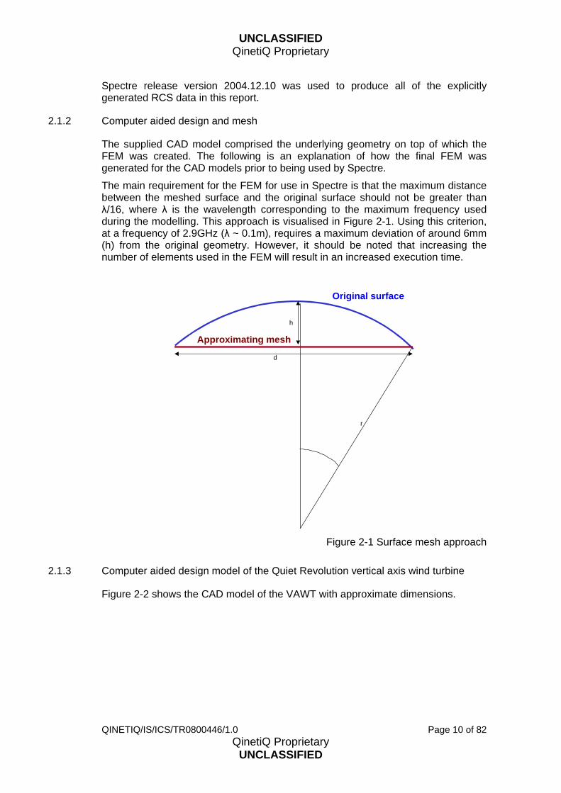
The main requirement for the FEM for use in Spectre is that the maximum distance between the meshed surface and the original surface should not be greater than λ/16, where λ is the wavelength corresponding to the maximum frequency used during the modelling. This approach is visualised in Figure 2-1. Using this criterion, at a frequency of 2.9GHz (λ ~ 0.1m), requires a maximum deviation of around 6mm (h) from the original geometry. However, it should be noted that increasing the number of elements used in the FEM will result in an increased execution time.
Figure 2-1 Surface mesh approach
2.1.3 Computer aided design model of the Quiet Revolution vertical axis wind turbine
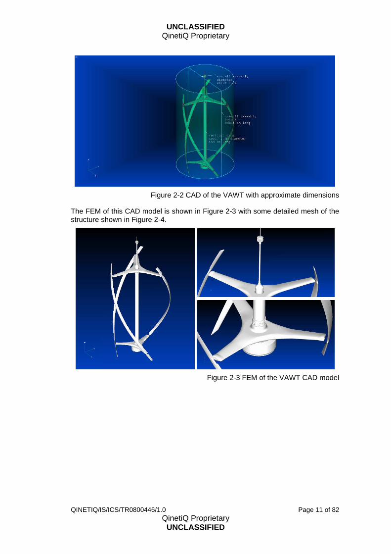
Figure 2-2 shows the CAD model of the VAWT with approximate dimensions.
h
r
d
Original surface
Approximating mesh
UNCLASSIFIED QinetiQ Proprietary
QINETIQ/IS/ICS/TR0800446/1.0 Page 11 of 82 QinetiQ Proprietary
UNCLASSIFIED
Figure 2-2 CAD of the VAWT with approximate dimensions
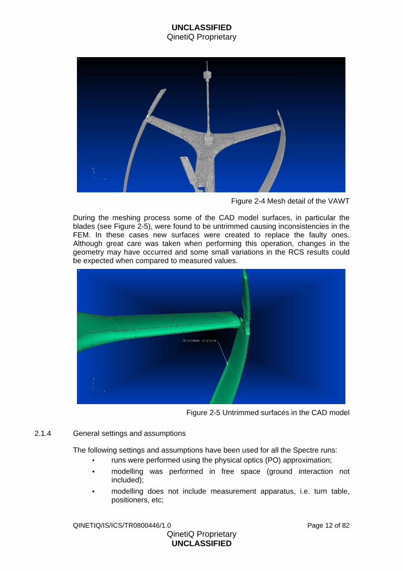
The FEM of this CAD model is shown in Figure 2-3 with some detailed mesh of the structure shown in Figure 2-4.
Figure 2-3 FEM of the VAWT CAD model
UNCLASSIFIED QinetiQ Proprietary
QINETIQ/IS/ICS/TR0800446/1.0 Page 12 of 82 QinetiQ Proprietary
UNCLASSIFIED
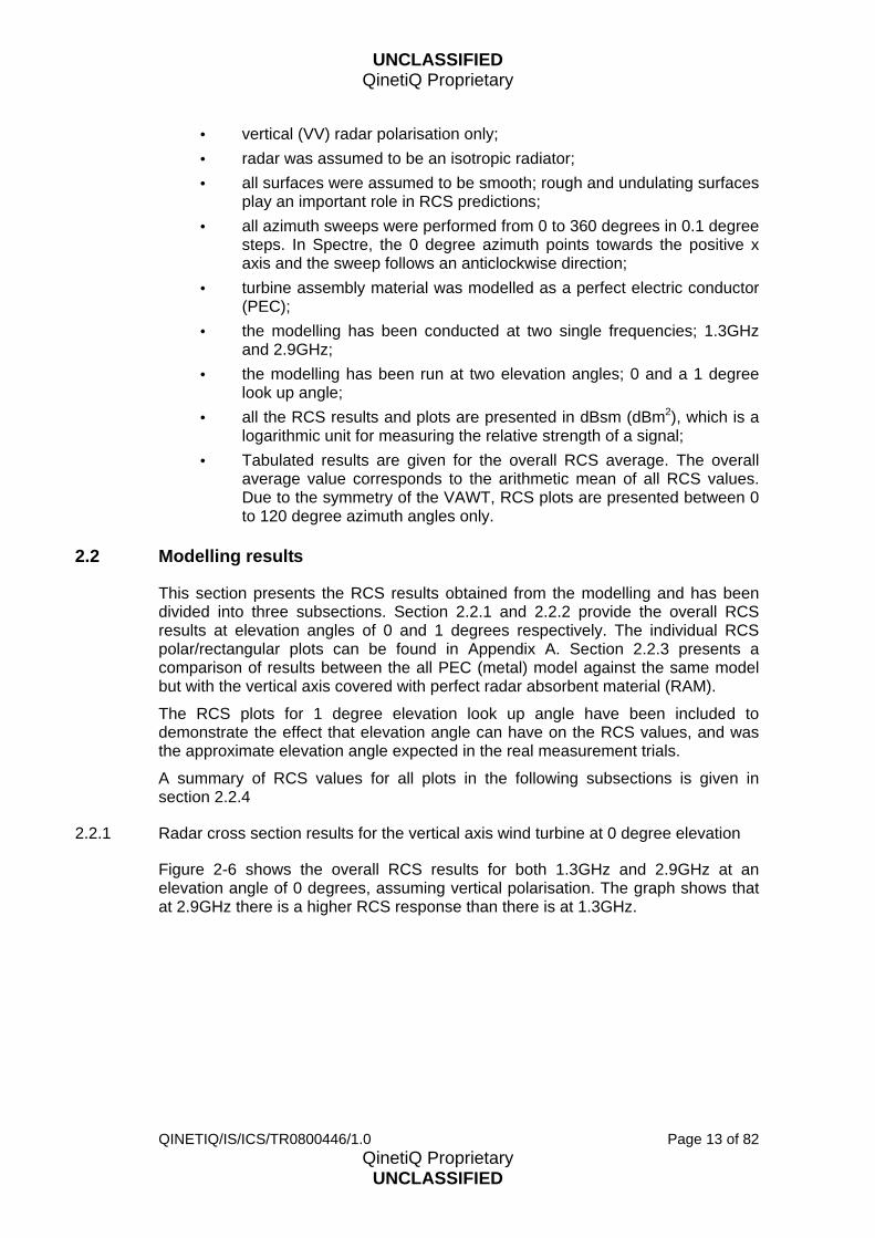
Figure 2-4 Mesh detail of the VAWT
During the meshing process some of the CAD model surfaces, in particular the blades (see Figure 2-5), were found to be untrimmed causing inconsistencies in the FEM. In these cases new surfaces were created to replace the faulty ones. Although great care was taken when performing this operation, changes in the geometry may have occurred and some small variations in the RCS results could be expected when compared to measured values.
Figure 2-5 Untrimmed surfaces in the CAD model
2.1.4 General settings and assumptions
The following settings and assumptions have been used for all the Spectre runs: • runs were performed using the physical optics (PO) approximation;
• modelling was performed in free space (ground interaction not included);
• modelling does not include measurement apparatus, i.e. turn table, positioners, etc;
UNCLASSIFIED QinetiQ Proprietary
QINETIQ/IS/ICS/TR0800446/1.0 Page 13 of 82 QinetiQ Proprietary
UNCLASSIFIED
• vertical (VV) radar polarisation only;
• radar was assumed to be an isotropic radiator;
• all surfaces were assumed to be smooth; rough and undulating surfaces play an important role in RCS predictions;
• all azimuth sweeps were performed from 0 to 360 degrees in 0.1 degree steps. In Spectre, the 0 degree azimuth points towards the positive x axis and the sweep follows an anticlockwise direction;
• turbine assembly material was modelled as a perfect electric conductor (PEC);
• the modelling has been conducted at two single frequencies; 1.3GHz and 2.9GHz;
• the modelling has been run at two elevation angles; 0 and a 1 degree look up angle;
• all the RCS results and plots are presented in dBsm (dBm2), which is a logarithmic unit for measuring the relative strength of a signal;
• Tabulated results are given for the overall RCS average. The overall average value corresponds to the arithmetic mean of all RCS values. Due to the symmetry of the VAWT, RCS plots are presented between 0 to 120 degree azimuth angles only.
2.2 Modelling results
This section presents the RCS results obtained from the modelling and has been divided into three subsections. Section 2.2.1 and 2.2.2 provide the overall RCS results at elevation angles of 0 and 1 degrees respectively. The individual RCS polar/rectangular plots can be found in Appendix A. Section 2.2.3 presents a comparison of results between the all PEC (metal) model against the same model but with the vertical axis covered with perfect radar absorbent material (RAM).
The RCS plots for 1 degree elevation look up angle have been included to demonstrate the effect that elevation angle can have on the RCS values, and was the approximate elevation angle expected in the real measurement trials.
A summary of RCS values for all plots in the following subsections is given in section 2.2.4
2.2.1 Radar cross section results for the vertical axis wind turbine at 0 degree elevation
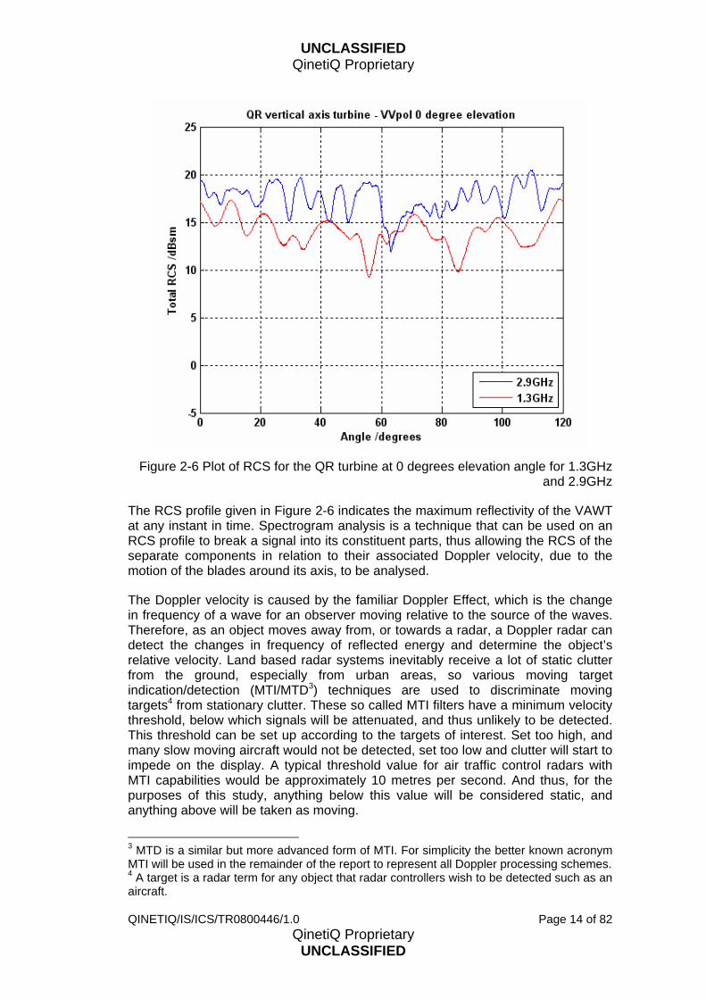
Figure 2-6 shows the overall RCS results for both 1.3GHz and 2.9GHz at an elevation angle of 0 degrees, assuming vertical polarisation. The graph shows that at 2.9GHz there is a higher RCS response than there is at 1.3GHz.
UNCLASSIFIED QinetiQ Proprietary
QINETIQ/IS/ICS/TR0800446/1.0 Page 14 of 82 QinetiQ Proprietary
UNCLASSIFIED
Figure 2-6 Plot of RCS for the QR turbine at 0 degrees elevation angle for 1.3GHz and 2.9GHz
The RCS profile given in Figure 2-6 indicates the maximum reflectivity of the VAWT at any instant in time. Spectrogram analysis is a technique that can be used on an RCS profile to break a signal into its constituent parts, thus allowing the RCS of the separate components in relation to their associated Doppler velocity, due to the motion of the blades around its axis, to be analysed.
The Doppler velocity is caused by the familiar Doppler Effect, which is the change in frequency of a wave for an observer moving relative to the source of the waves. Therefore, as an object moves away from, or towards a radar, a Doppler radar can detect the changes in frequency of reflected energy and determine the object’s relative velocity. Land based radar systems inevitably receive a lot of static clutter from the ground, especially from urban areas, so various moving target indication/detection (MTI/MTD3) techniques are used to discriminate moving targets4 from stationary clutter. These so called MTI filters have a minimum velocity threshold, below which signals will be attenuated, and thus unlikely to be detected. This threshold can be set up according to the targets of interest. Set too high, and many slow moving aircraft would not be detected, set too low and clutter will start to impede on the display. A typical threshold value for air traffic control radars with MTI capabilities would be approximately 10 metres per second. And thus, for the purposes of this study, anything below this value will be considered static, and anything above will be taken as moving.
3 MTD is a similar but more advanced form of MTI. For simplicity the better known acronym MTI will be used in the remainder of the report to represent all Doppler processing schemes. 4 A target is a radar term for any object that radar controllers wish to be detected such as an aircraft.
UNCLASSIFIED QinetiQ Proprietary
QINETIQ/IS/ICS/TR0800446/1.0 Page 15 of 82 QinetiQ Proprietary
UNCLASSIFIED
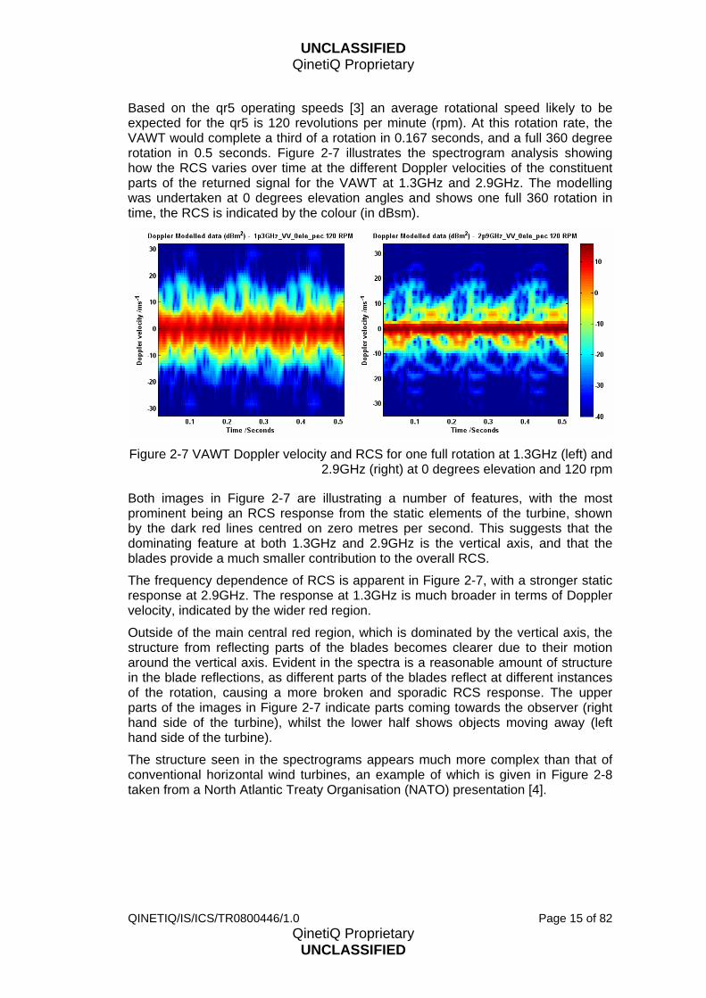
Based on the qr5 operating speeds [3] an average rotational speed likely to be expected for the qr5 is 120 revolutions per minute (rpm). At this rotation rate, the VAWT would complete a third of a rotation in 0.167 seconds, and a full 360 degree rotation in 0.5 seconds. Figure 2-7 illustrates the spectrogram analysis showing how the RCS varies over time at the different Doppler velocities of the constituent parts of the returned signal for the VAWT at 1.3GHz and 2.9GHz. The modelling was undertaken at 0 degrees elevation angles and shows one full 360 rotation in time, the RCS is indicated by the colour (in dBsm).
Figure 2-7 VAWT Doppler velocity and RCS for one full rotation at 1.3GHz (left) and 2.9GHz (right) at 0 degrees elevation and 120 rpm
Both images in Figure 2-7 are illustrating a number of features, with the most prominent being an RCS response from the static elements of the turbine, shown by the dark red lines centred on zero metres per second. This suggests that the dominating feature at both 1.3GHz and 2.9GHz is the vertical axis, and that the blades provide a much smaller contribution to the overall RCS.
The frequency dependence of RCS is apparent in Figure 2-7, with a stronger static response at 2.9GHz. The response at 1.3GHz is much broader in terms of Doppler velocity, indicated by the wider red region.
Outside of the main central red region, which is dominated by the vertical axis, the structure from reflecting parts of the blades becomes clearer due to their motion around the vertical axis. Evident in the spectra is a reasonable amount of structure in the blade reflections, as different parts of the blades reflect at different instances of the rotation, causing a more broken and sporadic RCS response. The upper parts of the images in Figure 2-7 indicate parts coming towards the observer (right hand side of the turbine), whilst the lower half shows objects moving away (left hand side of the turbine).
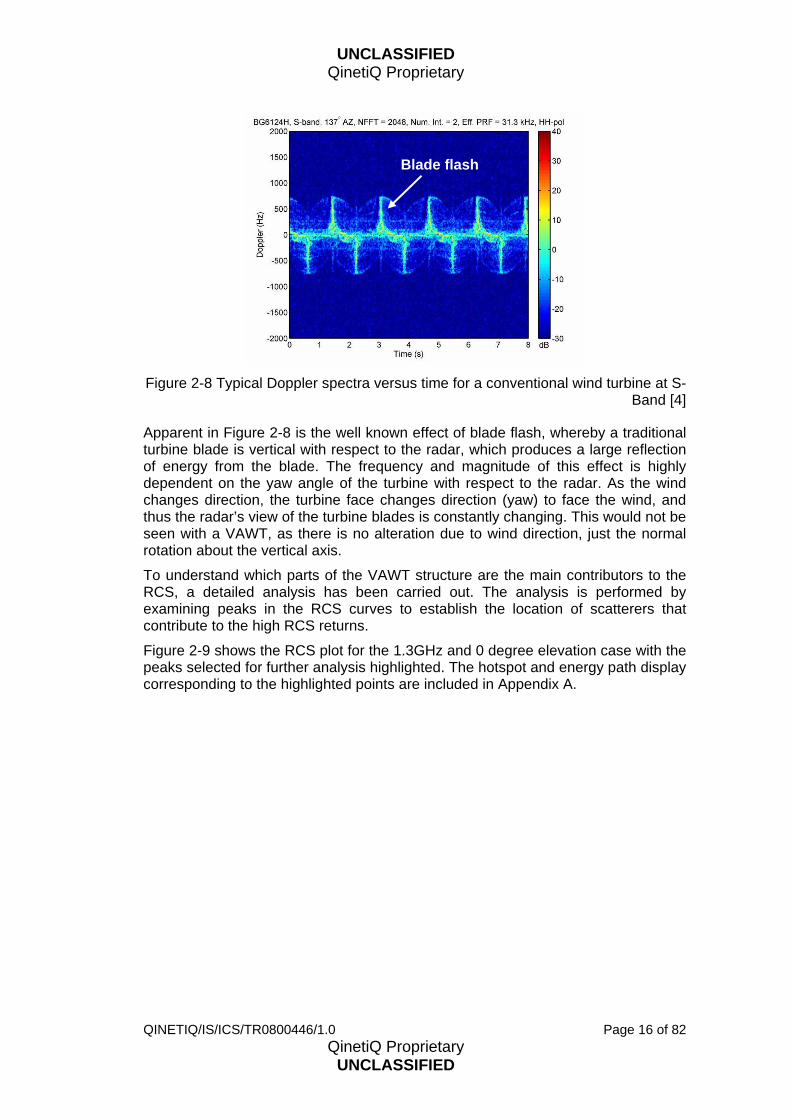
The structure seen in the spectrograms appears much more complex than that of conventional horizontal wind turbines, an example of which is given in Figure 2-8 taken from a North Atlantic Treaty Organisation (NATO) presentation [4].
UNCLASSIFIED QinetiQ Proprietary
QINETIQ/IS/ICS/TR0800446/1.0 Page 16 of 82 QinetiQ Proprietary
UNCLASSIFIED
Figure 2-8 Typical Doppler spectra versus time for a conventional wind turbine at S-Band [4]
Apparent in Figure 2-8 is the well known effect of blade flash, whereby a traditional turbine blade is vertical with respect to the radar, which produces a large reflection of energy from the blade. The frequency and magnitude of this effect is highly dependent on the yaw angle of the turbine with respect to the radar. As the wind changes direction, the turbine face changes direction (yaw) to face the wind, and thus the radar’s view of the turbine blades is constantly changing. This would not be seen with a VAWT, as there is no alteration due to wind direction, just the normal rotation about the vertical axis.
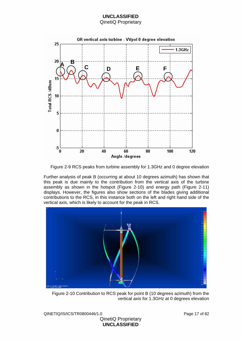
To understand which parts of the VAWT structure are the main contributors to the RCS, a detailed analysis has been carried out. The analysis is performed by examining peaks in the RCS curves to establish the location of scatterers that contribute to the high RCS returns.
Figure 2-9 shows the RCS plot for the 1.3GHz and 0 degree elevation case with the peaks selected for further analysis highlighted. The hotspot and energy path display corresponding to the highlighted points are included in Appendix A.
Blade flash
UNCLASSIFIED QinetiQ Proprietary
QINETIQ/IS/ICS/TR0800446/1.0 Page 17 of 82 QinetiQ Proprietary
UNCLASSIFIED
Figure 2-9 RCS peaks from turbine assembly for 1.3GHz and 0 degree elevation
Further analysis of peak B (occurring at about 10 degrees azimuth) has shown that this peak is due mainly to the contribution from the vertical axis of the turbine assembly as shown in the hotspot (Figure 2-10) and energy path (Figure 2-11) displays. However, the figures also show sections of the blades giving additional contributions to the RCS, in this instance both on the left and right hand side of the vertical axis, which is likely to account for the peak in RCS.
Figure 2-10 Contribution to RCS peak for point B (10 degrees azimuth) from the vertical axis for 1.3GHz at 0 degrees elevation
A F E D C
B
UNCLASSIFIED QinetiQ Proprietary
QINETIQ/IS/ICS/TR0800446/1.0 Page 18 of 82 QinetiQ Proprietary
UNCLASSIFIED
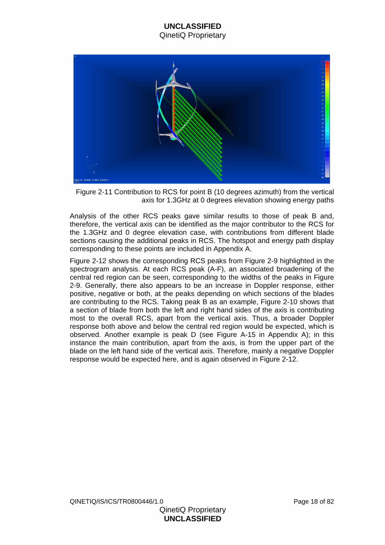
Figure 2-11 Contribution to RCS for point B (10 degrees azimuth) from the vertical axis for 1.3GHz at 0 degrees elevation showing energy paths
Analysis of the other RCS peaks gave similar results to those of peak B and, therefore, the vertical axis can be identified as the major contributor to the RCS for the 1.3GHz and 0 degree elevation case, with contributions from different blade sections causing the additional peaks in RCS. The hotspot and energy path display corresponding to these points are included in Appendix A.
Figure 2-12 shows the corresponding RCS peaks from Figure 2-9 highlighted in the spectrogram analysis. At each RCS peak (A-F), an associated broadening of the central red region can be seen, corresponding to the widths of the peaks in Figure 2-9. Generally, there also appears to be an increase in Doppler response, either positive, negative or both, at the peaks depending on which sections of the blades are contributing to the RCS. Taking peak B as an example, Figure 2-10 shows that a section of blade from both the left and right hand sides of the axis is contributing most to the overall RCS, apart from the vertical axis. Thus, a broader Doppler response both above and below the central red region would be expected, which is observed. Another example is peak D (see Figure A-15 in Appendix A); in this instance the main contribution, apart from the axis, is from the upper part of the blade on the left hand side of the vertical axis. Therefore, mainly a negative Doppler response would be expected here, and is again observed in Figure 2-12.
UNCLASSIFIED QinetiQ Proprietary
QINETIQ/IS/ICS/TR0800446/1.0 Page 19 of 82 QinetiQ Proprietary
UNCLASSIFIED
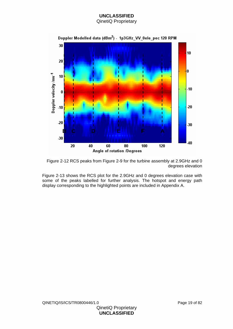
Figure 2-12 RCS peaks from Figure 2-9 for the turbine assembly at 2.9GHz and 0 degrees elevation
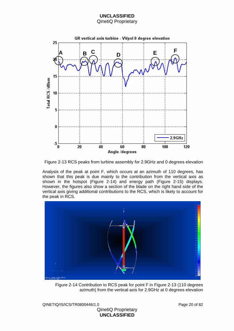
Figure 2-13 shows the RCS plot for the 2.9GHz and 0 degrees elevation case with some of the peaks labelled for further analysis. The hotspot and energy path display corresponding to the highlighted points are included in Appendix A.
A F E D C B
UNCLASSIFIED QinetiQ Proprietary
QINETIQ/IS/ICS/TR0800446/1.0 Page 20 of 82 QinetiQ Proprietary
UNCLASSIFIED
Figure 2-13 RCS peaks from turbine assembly for 2.9GHz and 0 degrees elevation
Analysis of the peak at point F, which occurs at an azimuth of 110 degrees, has shown that this peak is due mainly to the contribution from the vertical axis as shown in the hotspot (Figure 2-14) and energy path (Figure 2-15) displays. However, the figures also show a section of the blade on the right hand side of the vertical axis giving additional contributions to the RCS, which is likely to account for the peak in RCS.
Figure 2-14 Contribution to RCS peak for point F in Figure 2-13 (110 degrees azimuth) from the vertical axis for 2.9GHz at 0 degrees elevation
A F E D C B
UNCLASSIFIED QinetiQ Proprietary
QINETIQ/IS/ICS/TR0800446/1.0 Page 21 of 82 QinetiQ Proprietary
UNCLASSIFIED
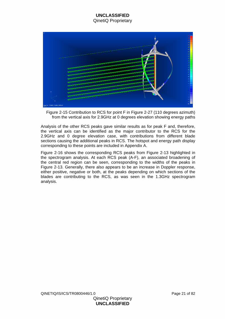
Figure 2-15 Contribution to RCS for point F in Figure 2-27 (110 degrees azimuth) from the vertical axis for 2.9GHz at 0 degrees elevation showing energy paths
Analysis of the other RCS peaks gave similar results as for peak F and, therefore, the vertical axis can be identified as the major contributor to the RCS for the 2.9GHz and 0 degree elevation case, with contributions from different blade sections causing the additional peaks in RCS. The hotspot and energy path display corresponding to these points are included in Appendix A.
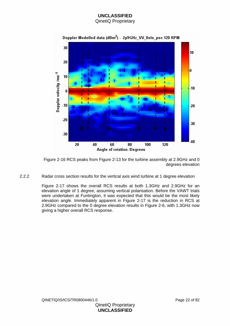
Figure 2-16 shows the corresponding RCS peaks from Figure 2-13 highlighted in the spectrogram analysis. At each RCS peak (A-F), an associated broadening of the central red region can be seen, corresponding to the widths of the peaks in Figure 2-13. Generally, there also appears to be an increase in Doppler response, either positive, negative or both, at the peaks depending on which sections of the blades are contributing to the RCS, as was seen in the 1.3GHz spectrogram analysis.
UNCLASSIFIED QinetiQ Proprietary
QINETIQ/IS/ICS/TR0800446/1.0 Page 22 of 82 QinetiQ Proprietary
UNCLASSIFIED
Figure 2-16 RCS peaks from Figure 2-13 for the turbine assembly at 2.9GHz and 0 degrees elevation
2.2.2 Radar cross section results for the vertical axis wind turbine at 1 degree elevation
Figure 2-17 shows the overall RCS results at both 1.3GHz and 2.9GHz for an elevation angle of 1 degree, assuming vertical polarisation. Before the VAWT trials were undertaken at Funtington, it was expected that this would be the most likely elevation angle. Immediately apparent in Figure 2-17 is the reduction in RCS at 2.9GHz compared to the 0 degree elevation results in Figure 2-6, with 1.3GHz now giving a higher overall RCS response.
A F E D C B
UNCLASSIFIED QinetiQ Proprietary
QINETIQ/IS/ICS/TR0800446/1.0 Page 23 of 82 QinetiQ Proprietary
UNCLASSIFIED
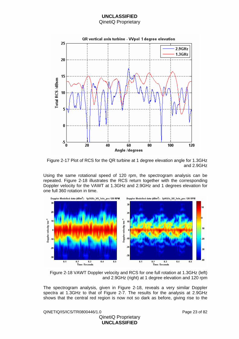
Figure 2-17 Plot of RCS for the QR turbine at 1 degree elevation angle for 1.3GHz and 2.9GHz
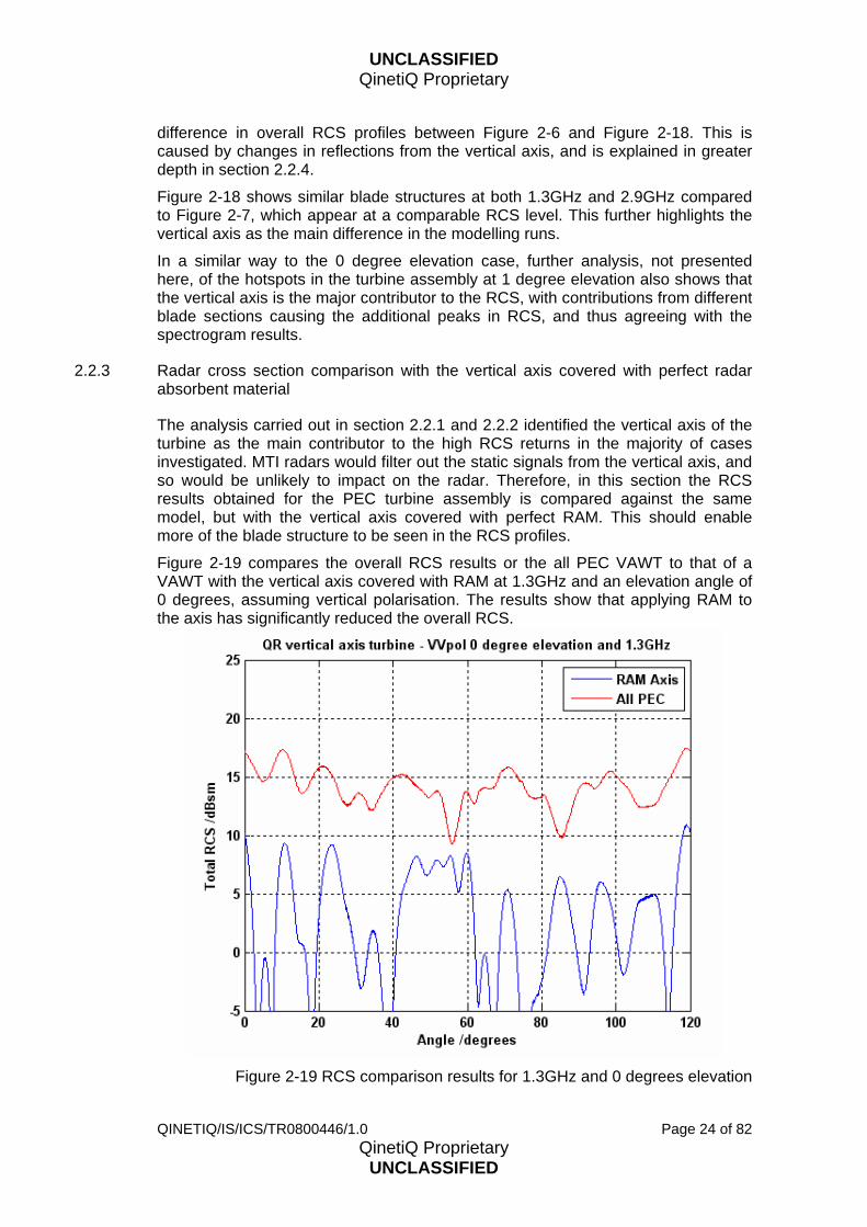
Using the same rotational speed of 120 rpm, the spectrogram analysis can be repeated. Figure 2-18 illustrates the RCS return together with the corresponding Doppler velocity for the VAWT at 1.3GHz and 2.9GHz and 1 degrees elevation for one full 360 rotation in time.
Figure 2-18 VAWT Doppler velocity and RCS for one full rotation at 1.3GHz (left) and 2.9GHz (right) at 1 degree elevation and 120 rpm
The spectrogram analysis, given in Figure 2-18, reveals a very similar Doppler spectra at 1.3GHz to that of Figure 2-7. The results for the analysis at 2.9GHz shows that the central red region is now not so dark as before, giving rise to the
UNCLASSIFIED QinetiQ Proprietary
QINETIQ/IS/ICS/TR0800446/1.0 Page 24 of 82 QinetiQ Proprietary
UNCLASSIFIED
difference in overall RCS profiles between Figure 2-6 and Figure 2-18. This is caused by changes in reflections from the vertical axis, and is explained in greater depth in section 2.2.4.
Figure 2-18 shows similar blade structures at both 1.3GHz and 2.9GHz compared to Figure 2-7, which appear at a comparable RCS level. This further highlights the vertical axis as the main difference in the modelling runs.
In a similar way to the 0 degree elevation case, further analysis, not presented here, of the hotspots in the turbine assembly at 1 degree elevation also shows that the vertical axis is the major contributor to the RCS, with contributions from different blade sections causing the additional peaks in RCS, and thus agreeing with the spectrogram results.
2.2.3 Radar cross section comparison with the vertical axis covered with perfect radar absorbent material
The analysis carried out in section 2.2.1 and 2.2.2 identified the vertical axis of the turbine as the main contributor to the high RCS returns in the majority of cases investigated. MTI radars would filter out the static signals from the vertical axis, and so would be unlikely to impact on the radar. Therefore, in this section the RCS results obtained for the PEC turbine assembly is compared against the same model, but with the vertical axis covered with perfect RAM. This should enable more of the blade structure to be seen in the RCS profiles.
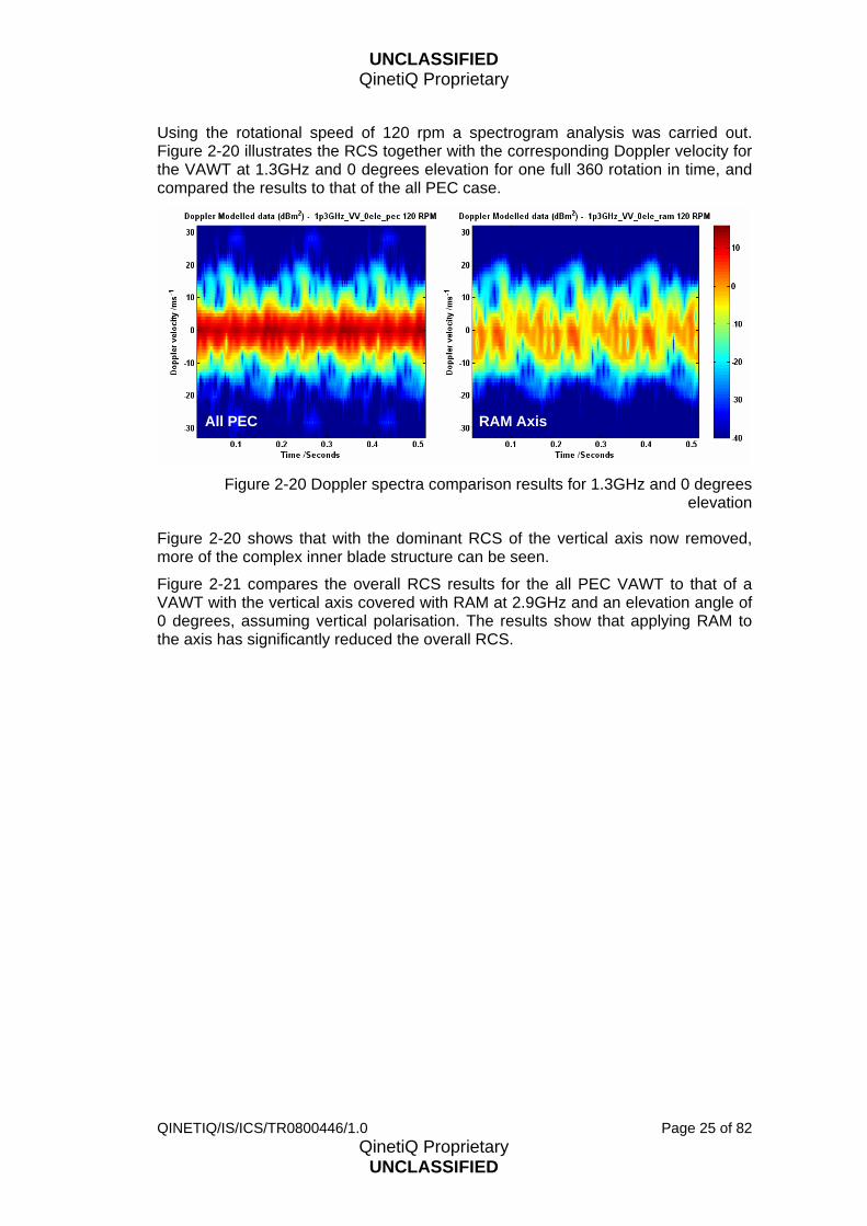
Figure 2-19 compares the overall RCS results or the all PEC VAWT to that of a VAWT with the vertical axis covered with RAM at 1.3GHz and an elevation angle of 0 degrees, assuming vertical polarisation. The results show that applying RAM to the axis has significantly reduced the overall RCS.
Figure 2-19 RCS comparison results for 1.3GHz and 0 degrees elevation
UNCLASSIFIED QinetiQ Proprietary
QINETIQ/IS/ICS/TR0800446/1.0 Page 25 of 82 QinetiQ Proprietary
UNCLASSIFIED
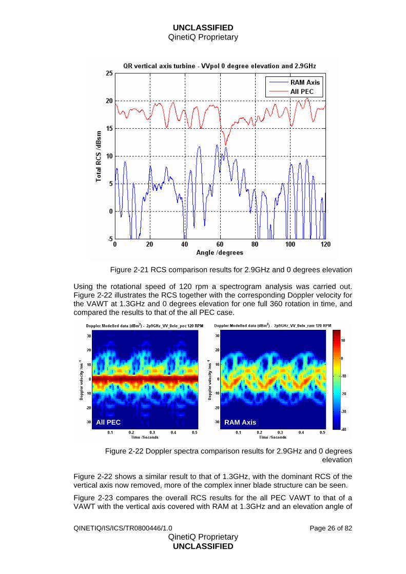
Using the rotational speed of 120 rpm a spectrogram analysis was carried out. Figure 2-20 illustrates the RCS together with the corresponding Doppler velocity for the VAWT at 1.3GHz and 0 degrees elevation for one full 360 rotation in time, and compared the results to that of the all PEC case.
Figure 2-20 Doppler spectra comparison results for 1.3GHz and 0 degrees elevation
Figure 2-20 shows that with the dominant RCS of the vertical axis now removed, more of the complex inner blade structure can be seen.
Figure 2-21 compares the overall RCS results for the all PEC VAWT to that of a VAWT with the vertical axis covered with RAM at 2.9GHz and an elevation angle of 0 degrees, assuming vertical polarisation. The results show that applying RAM to the axis has significantly reduced the overall RCS.
All PEC RAM Axis
UNCLASSIFIED QinetiQ Proprietary
QINETIQ/IS/ICS/TR0800446/1.0 Page 26 of 82 QinetiQ Proprietary
UNCLASSIFIED
Figure 2-21 RCS comparison results for 2.9GHz and 0 degrees elevation
Using the rotational speed of 120 rpm a spectrogram analysis was carried out. Figure 2-22 illustrates the RCS together with the corresponding Doppler velocity for the VAWT at 1.3GHz and 0 degrees elevation for one full 360 rotation in time, and compared the results to that of the all PEC case.
Figure 2-22 Doppler spectra comparison results for 2.9GHz and 0 degrees elevation
Figure 2-22 shows a similar result to that of 1.3GHz, with the dominant RCS of the vertical axis now removed, more of the complex inner blade structure can be seen.
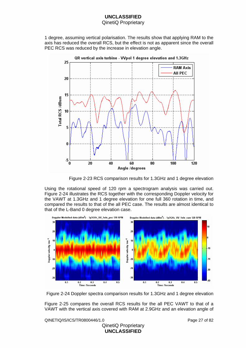
Figure 2-23 compares the overall RCS results for the all PEC VAWT to that of a VAWT with the vertical axis covered with RAM at 1.3GHz and an elevation angle of
All PEC RAM Axis
UNCLASSIFIED QinetiQ Proprietary
QINETIQ/IS/ICS/TR0800446/1.0 Page 27 of 82 QinetiQ Proprietary
UNCLASSIFIED
1 degree, assuming vertical polarisation. The results show that applying RAM to the axis has reduced the overall RCS, but the effect is not as apparent since the overall PEC RCS was reduced by the increase in elevation angle.
Figure 2-23 RCS comparison results for 1.3GHz and 1 degree elevation
Using the rotational speed of 120 rpm a spectrogram analysis was carried out. Figure 2-24 illustrates the RCS together with the corresponding Doppler velocity for the VAWT at 1.3GHz and 1 degree elevation for one full 360 rotation in time, and compared the results to that of the all PEC case. The results are almost identical to that of the L-Band 0 degree elevation case.
Figure 2-24 Doppler spectra comparison results for 1.3GHz and 1 degree elevation
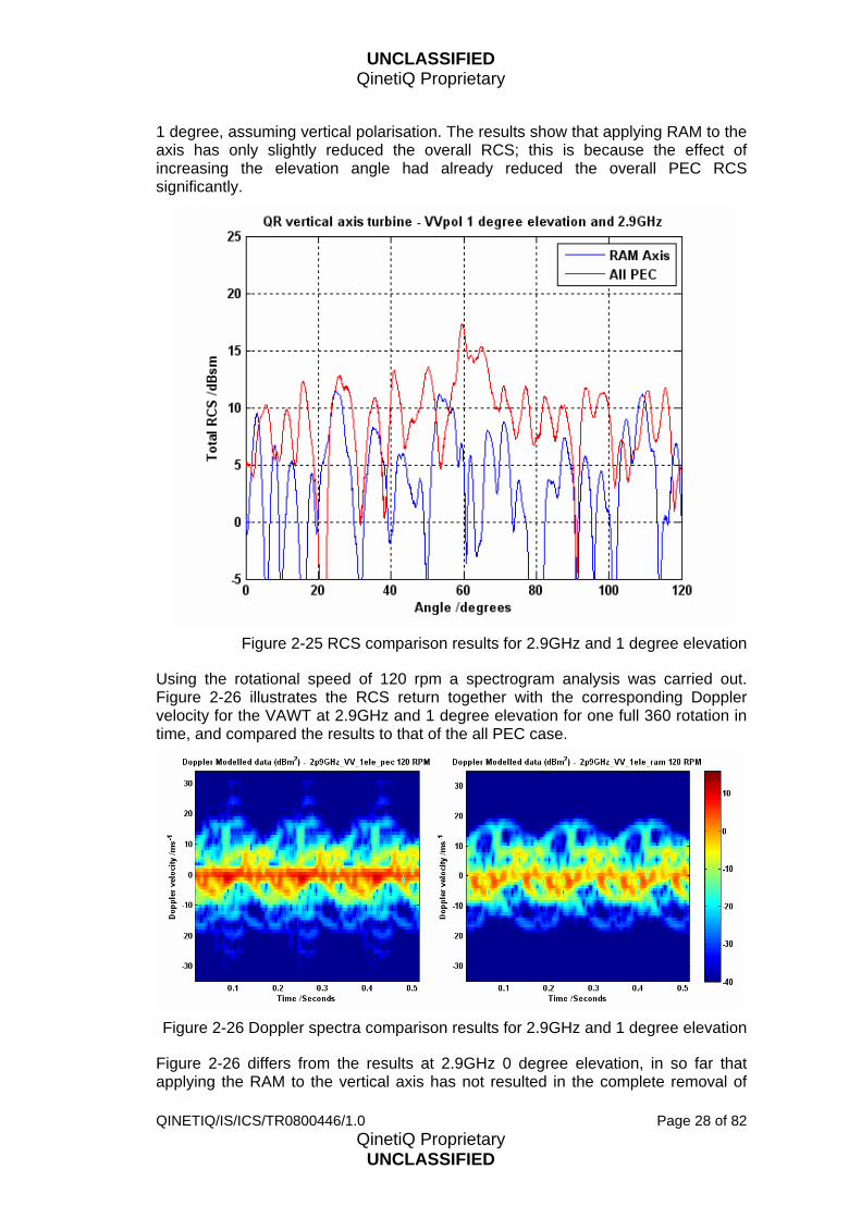
Figure 2-25 compares the overall RCS results for the all PEC VAWT to that of a VAWT with the vertical axis covered with RAM at 2.9GHz and an elevation angle of
UNCLASSIFIED QinetiQ Proprietary
QINETIQ/IS/ICS/TR0800446/1.0 Page 28 of 82 QinetiQ Proprietary
UNCLASSIFIED
1 degree, assuming vertical polarisation. The results show that applying RAM to the axis has only slightly reduced the overall RCS; this is because the effect of increasing the elevation angle had already reduced the overall PEC RCS significantly.
Figure 2-25 RCS comparison results for 2.9GHz and 1 degree elevation
Using the rotational speed of 120 rpm a spectrogram analysis was carried out. Figure 2-26 illustrates the RCS return together with the corresponding Doppler velocity for the VAWT at 2.9GHz and 1 degree elevation for one full 360 rotation in time, and compared the results to that of the all PEC case.
Figure 2-26 Doppler spectra comparison results for 2.9GHz and 1 degree elevation
Figure 2-26 differs from the results at 2.9GHz 0 degree elevation, in so far that applying the RAM to the vertical axis has not resulted in the complete removal of
UNCLASSIFIED QinetiQ Proprietary
QINETIQ/IS/ICS/TR0800446/1.0 Page 29 of 82 QinetiQ Proprietary
UNCLASSIFIED
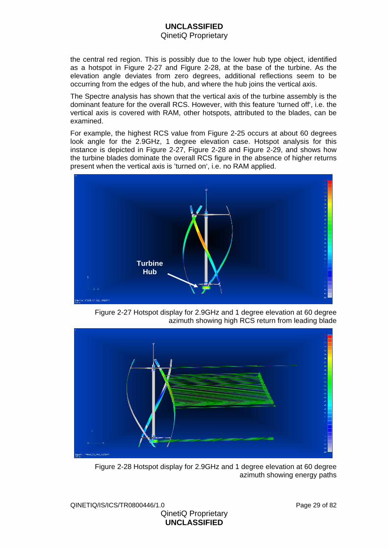
the central red region. This is possibly due to the lower hub type object, identified as a hotspot in Figure 2-27 and Figure 2-28, at the base of the turbine. As the elevation angle deviates from zero degrees, additional reflections seem to be occurring from the edges of the hub, and where the hub joins the vertical axis.
The Spectre analysis has shown that the vertical axis of the turbine assembly is the dominant feature for the overall RCS. However, with this feature ’turned off‘, i.e. the vertical axis is covered with RAM, other hotspots, attributed to the blades, can be examined.
For example, the highest RCS value from Figure 2-25 occurs at about 60 degrees look angle for the 2.9GHz, 1 degree elevation case. Hotspot analysis for this instance is depicted in Figure 2-27, Figure 2-28 and Figure 2-29, and shows how the turbine blades dominate the overall RCS figure in the absence of higher returns present when the vertical axis is ’turned on‘, i.e. no RAM applied.
Figure 2-27 Hotspot display for 2.9GHz and 1 degree elevation at 60 degree azimuth showing high RCS return from leading blade
Figure 2-28 Hotspot display for 2.9GHz and 1 degree elevation at 60 degree azimuth showing energy paths
Turbine Hub
UNCLASSIFIED QinetiQ Proprietary
QINETIQ/IS/ICS/TR0800446/1.0 Page 30 of 82 QinetiQ Proprietary
UNCLASSIFIED
Figure 2-29 Hotspot display for 2.9GHz and 1 degree elevation at 60 degree azimuth highest RCS hotspot located at blade-axis junction
2.2.4 Summary of Spectre radar cross section modelling
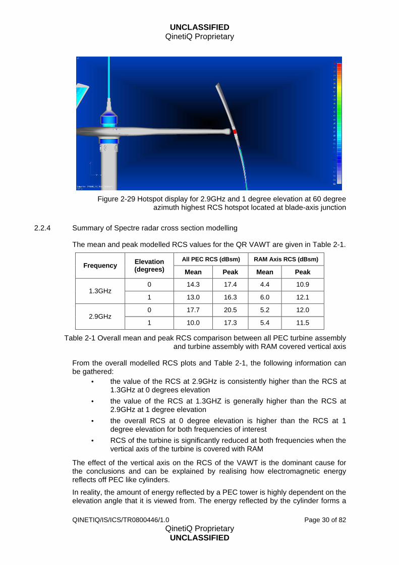
The mean and peak modelled RCS values for the QR VAWT are given in Table 2-1.
All PEC RCS (dBsm) RAM Axis RCS (dBsm) Frequency Elevation
(degrees) Mean Peak Mean Peak
0 14.3 17.4 4.4 10.9 1.3GHz
1 13.0 16.3 6.0 12.1
0 17.7 20.5 5.2 12.0 2.9GHz
1 10.0 17.3 5.4 11.5
Table 2-1 Overall mean and peak RCS comparison between all PEC turbine assembly and turbine assembly with RAM covered vertical axis
From the overall modelled RCS plots and Table 2-1, the following information can be gathered:
• the value of the RCS at 2.9GHz is consistently higher than the RCS at 1.3GHz at 0 degrees elevation
• the value of the RCS at 1.3GHZ is generally higher than the RCS at 2.9GHz at 1 degree elevation
• the overall RCS at 0 degree elevation is higher than the RCS at 1 degree elevation for both frequencies of interest
• RCS of the turbine is significantly reduced at both frequencies when the vertical axis of the turbine is covered with RAM
The effect of the vertical axis on the RCS of the VAWT is the dominant cause for the conclusions and can be explained by realising how electromagnetic energy reflects off PEC like cylinders.
In reality, the amount of energy reflected by a PEC tower is highly dependent on the elevation angle that it is viewed from. The energy reflected by the cylinder forms a
UNCLASSIFIED QinetiQ Proprietary
QINETIQ/IS/ICS/TR0800446/1.0 Page 31 of 82 QinetiQ Proprietary
UNCLASSIFIED
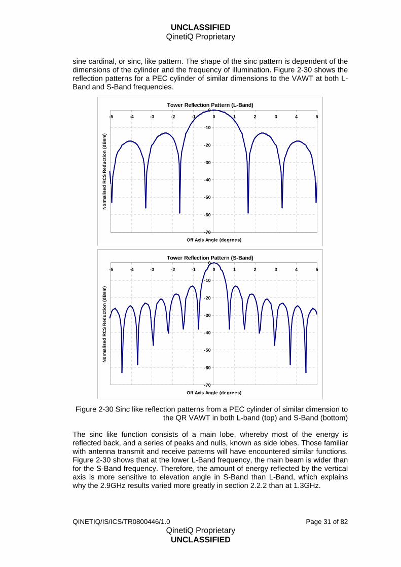
sine cardinal, or sinc, like pattern. The shape of the sinc pattern is dependent of the dimensions of the cylinder and the frequency of illumination. Figure 2-30 shows the reflection patterns for a PEC cylinder of similar dimensions to the VAWT at both L-Band and S-Band frequencies.
Tower Reflection Pattern (L-Band)
-70
-60
-50
-40
-30
-20
-10
0-5 -4 -3 -2 -1 0 1 2 3 4 5
Off Axis Angle (degrees)
Nor
mal
ised
RC
S R
educ
tion
(dB
sm)
Tower Reflection Pattern (S-Band)
-70
-60
-50
-40
-30
-20
-10
0-5 -4 -3 -2 -1 0 1 2 3 4 5
Off Axis Angle (degrees)
Nor
mal
ised
RC
S R
educ
tion
(dB
sm)
Figure 2-30 Sinc like reflection patterns from a PEC cylinder of similar dimension to the QR VAWT in both L-band (top) and S-Band (bottom)
The sinc like function consists of a main lobe, whereby most of the energy is reflected back, and a series of peaks and nulls, known as side lobes. Those familiar with antenna transmit and receive patterns will have encountered similar functions. Figure 2-30 shows that at the lower L-Band frequency, the main beam is wider than for the S-Band frequency. Therefore, the amount of energy reflected by the vertical axis is more sensitive to elevation angle in S-Band than L-Band, which explains why the 2.9GHz results varied more greatly in section 2.2.2 than at 1.3GHz.
UNCLASSIFIED QinetiQ Proprietary
QINETIQ/IS/ICS/TR0800446/1.0 Page 32 of 82 QinetiQ Proprietary
UNCLASSIFIED
Taking values from the graphs in Figure 2-30 as an example, at one degree elevation angle, the amount of signal reduction in L-Band is approximately 6dB, compared to a reduction of 13dB in S-Band, in reference to the level of the main lobe. One point to note here is that in S-Band, the first side lobe dominates the reflection at 1 degree elevation rather than the main lobe.
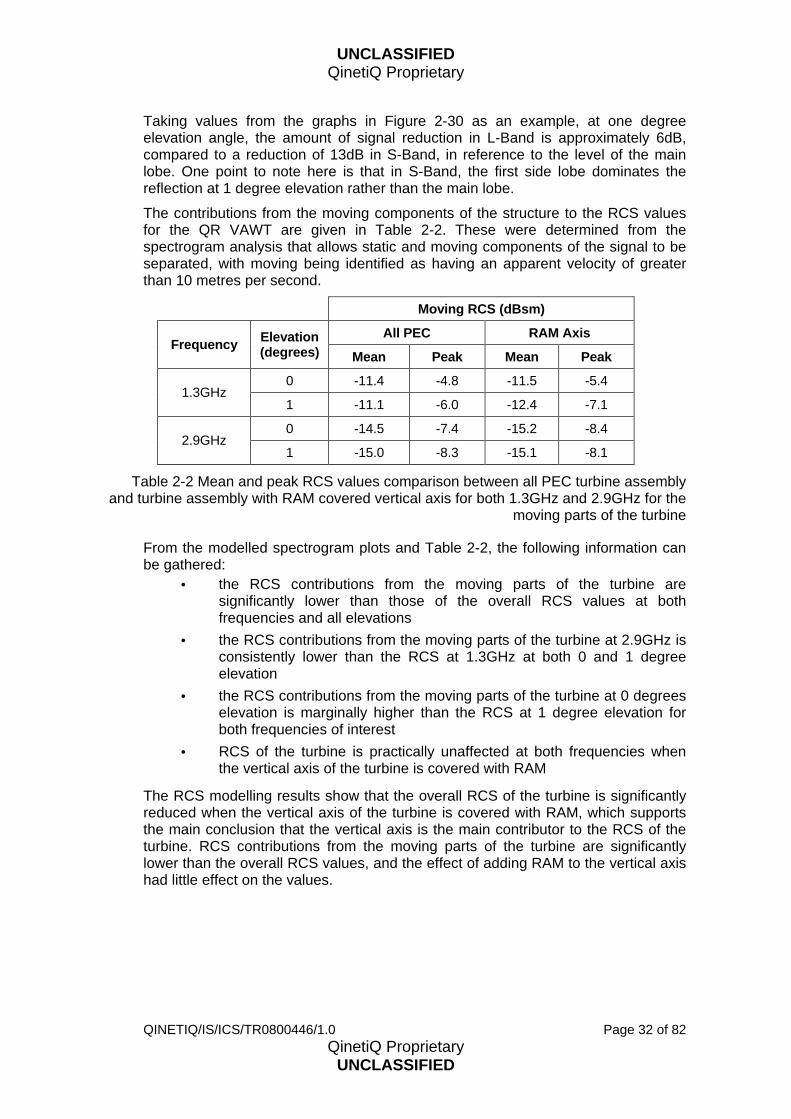
The contributions from the moving components of the structure to the RCS values for the QR VAWT are given in Table 2-2. These were determined from the spectrogram analysis that allows static and moving components of the signal to be separated, with moving being identified as having an apparent velocity of greater than 10 metres per second.
Moving RCS (dBsm)
All PEC RAM Axis Frequency Elevation
(degrees) Mean Peak Mean Peak
0 -11.4 -4.8 -11.5 -5.4 1.3GHz
1 -11.1 -6.0 -12.4 -7.1
0 -14.5 -7.4 -15.2 -8.4 2.9GHz
1 -15.0 -8.3 -15.1 -8.1
Table 2-2 Mean and peak RCS values comparison between all PEC turbine assembly and turbine assembly with RAM covered vertical axis for both 1.3GHz and 2.9GHz for the
moving parts of the turbine
From the modelled spectrogram plots and Table 2-2, the following information can be gathered:
• the RCS contributions from the moving parts of the turbine are significantly lower than those of the overall RCS values at both frequencies and all elevations
• the RCS contributions from the moving parts of the turbine at 2.9GHz is consistently lower than the RCS at 1.3GHz at both 0 and 1 degree elevation
• the RCS contributions from the moving parts of the turbine at 0 degrees elevation is marginally higher than the RCS at 1 degree elevation for both frequencies of interest
• RCS of the turbine is practically unaffected at both frequencies when the vertical axis of the turbine is covered with RAM
The RCS modelling results show that the overall RCS of the turbine is significantly reduced when the vertical axis of the turbine is covered with RAM, which supports the main conclusion that the vertical axis is the main contributor to the RCS of the turbine. RCS contributions from the moving parts of the turbine are significantly lower than the overall RCS values, and the effect of adding RAM to the vertical axis had little effect on the values.
UNCLASSIFIED QinetiQ Proprietary
QINETIQ/IS/ICS/TR0800446/1.0 Page 33 of 82 QinetiQ Proprietary
UNCLASSIFIED
3 Vertical Axis Wind Turbine Measurements and Analysis This section reports on the real measurement trials of the VAWT. Little is known about the possible impact of a VAWT on radar, and being relatively small in size compared to a traditional large scale horizontal axis wind turbine, there is the potential to erect many within a small area. To approach the concerns surrounding the potential impact of a VAWT on radar operations, the RCS of a QR VAWT was measured.
3.1 Installation and set up
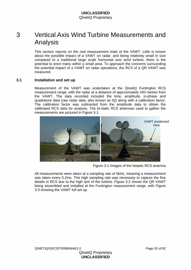
Measurement of the VAWT was undertaken at the QinetiQ Funtington RCS measurement range, with the radar at a distance of approximately 240 metres from the VAWT. The data recorded included the time, amplitude, in-phase and quadrature data (raw radar data, also known as IQ) along with a calibration factor. The calibration factor was subtracted from the amplitude data to obtain the calibrated RCS data for analysis. The bi-static RCS antennas used to gather the measurements are pictured in Figure 3-1.
Figure 3-1 Images of the bistatic RCS antenna
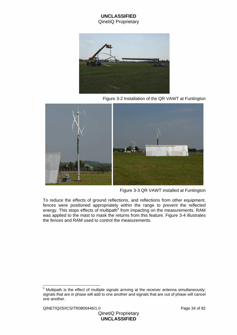
All measurements were taken at a sampling rate of 5kHz, meaning a measurement was taken every 0.2ms. This high sampling rate was necessary to capture the fine details in RCS due to the high rpm of the turbine. Figure 3-2 shows the QR VAWT being assembled and installed at the Funtington measurement range, with Figure 3-3 showing the VAWT full set up.
VAWT positioned here
UNCLASSIFIED QinetiQ Proprietary
QINETIQ/IS/ICS/TR0800446/1.0 Page 34 of 82 QinetiQ Proprietary
UNCLASSIFIED
Figure 3-2 Installation of the QR VAWT at Funtington
Figure 3-3 QR VAWT installed at Funtington
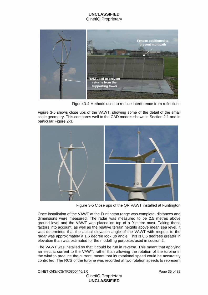
To reduce the effects of ground reflections, and reflections from other equipment, fences were positioned appropriately within the range to prevent the reflected energy. This stops effects of multipath5 from impacting on the measurements. RAM was applied to the mast to mask the returns from this feature. Figure 3-4 illustrates the fences and RAM used to control the measurements.
5 Multipath is the effect of multiple signals arriving at the receiver antenna simultaneously; signals that are in phase will add to one another and signals that are out of phase will cancel one another.
UNCLASSIFIED QinetiQ Proprietary
QINETIQ/IS/ICS/TR0800446/1.0 Page 35 of 82 QinetiQ Proprietary
UNCLASSIFIED
Figure 3-4 Methods used to reduce interference from reflections
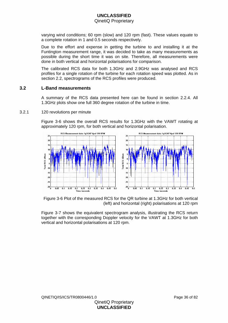
Figure 3-5 shows close ups of the VAWT, showing some of the detail of the small scale geometry. This compares well to the CAD models shown in Section 2.1 and in particular Figure 2-3.
Figure 3-5 Close ups of the QR VAWT installed at Funtington
Once installation of the VAWT at the Funtington range was complete, distances and dimensions were measured. The radar was measured to be 2.5 metres above ground level and the VAWT was placed on top of a 9 metre mast. Taking these factors into account, as well as the relative terrain heights above mean sea level, it was determined that the actual elevation angle of the VAWT with respect to the radar was approximately a 1.6 degree look up angle. This is 0.6 degrees greater in elevation than was estimated for the modelling purposes used in section 2.
The VAWT was installed so that it could be run in reverse. This meant that applying an electric current to the VAWT, rather than allowing the rotation of the turbine in the wind to produce the current, meant that its rotational speed could be accurately controlled. The RCS of the turbine was recorded at two rotation speeds to represent
RAM used to prevent returns from the supporting tower
Fences positioned to prevent multipath
UNCLASSIFIED QinetiQ Proprietary
QINETIQ/IS/ICS/TR0800446/1.0 Page 36 of 82 QinetiQ Proprietary
UNCLASSIFIED
varying wind conditions; 60 rpm (slow) and 120 rpm (fast). These values equate to a complete rotation in 1 and 0.5 seconds respectively.
Due to the effort and expense in getting the turbine to and installing it at the Funtington measurement range, it was decided to take as many measurements as possible during the short time it was on site. Therefore, all measurements were done in both vertical and horizontal polarisations for comparison.
The calibrated RCS data for both 1.3GHz and 2.9GHz was analysed and RCS profiles for a single rotation of the turbine for each rotation speed was plotted. As in section 2.2, spectrograms of the RCS profiles were produced.
3.2 L-Band measurements
A summary of the RCS data presented here can be found in section 2.2.4. All 1.3GHz plots show one full 360 degree rotation of the turbine in time.
3.2.1 120 revolutions per minute
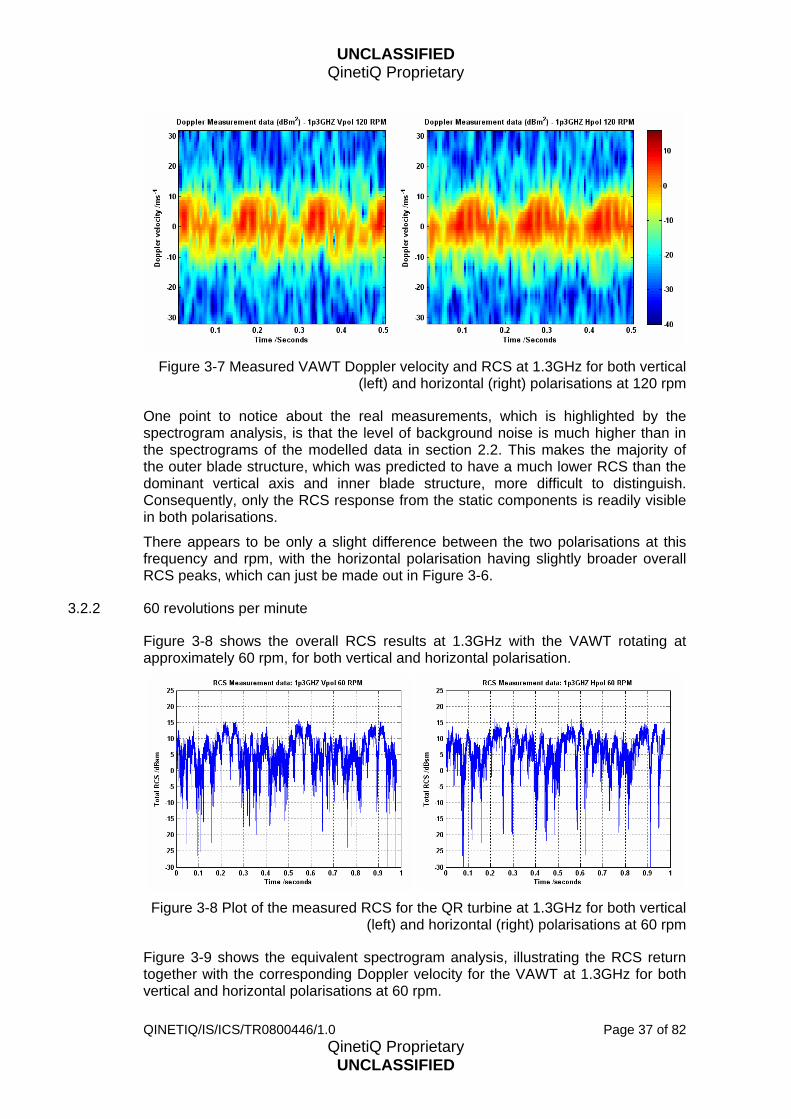
Figure 3-6 shows the overall RCS results for 1.3GHz with the VAWT rotating at approximately 120 rpm, for both vertical and horizontal polarisation.
Figure 3-6 Plot of the measured RCS for the QR turbine at 1.3GHz for both vertical (left) and horizontal (right) polarisations at 120 rpm
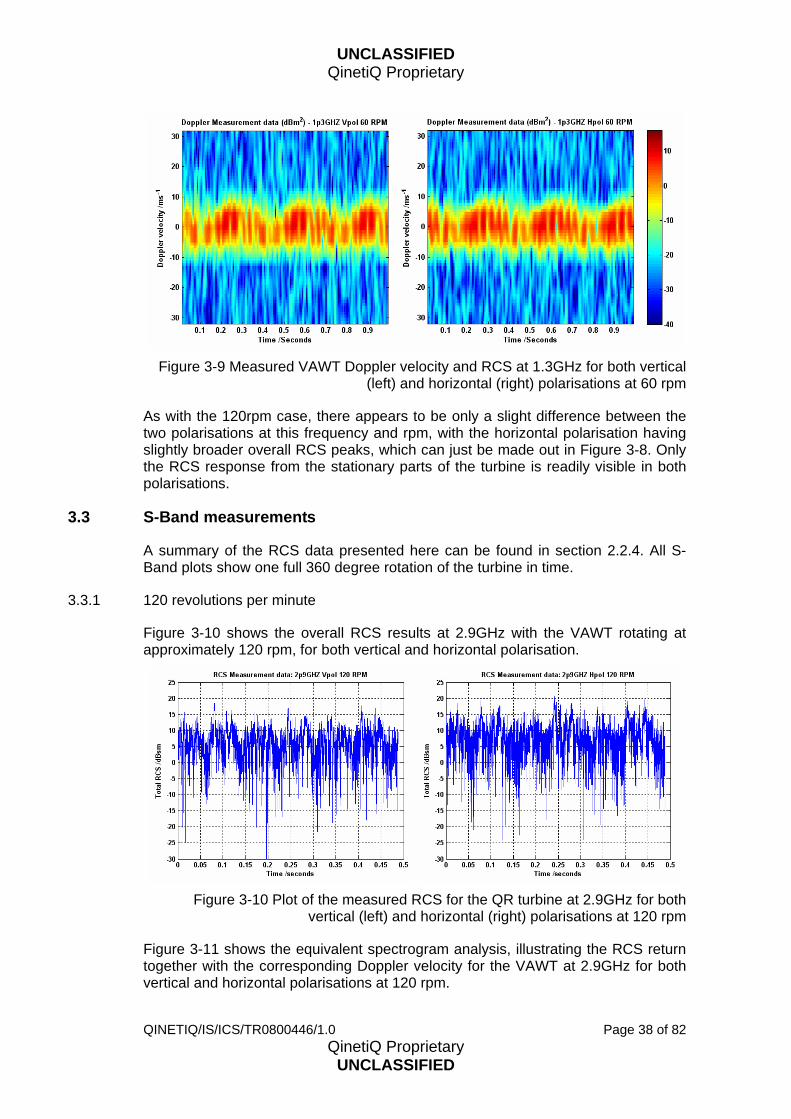
Figure 3-7 shows the equivalent spectrogram analysis, illustrating the RCS return together with the corresponding Doppler velocity for the VAWT at 1.3GHz for both vertical and horizontal polarisations at 120 rpm.
UNCLASSIFIED QinetiQ Proprietary
QINETIQ/IS/ICS/TR0800446/1.0 Page 37 of 82 QinetiQ Proprietary
UNCLASSIFIED
Figure 3-7 Measured VAWT Doppler velocity and RCS at 1.3GHz for both vertical (left) and horizontal (right) polarisations at 120 rpm
One point to notice about the real measurements, which is highlighted by the spectrogram analysis, is that the level of background noise is much higher than in the spectrograms of the modelled data in section 2.2. This makes the majority of the outer blade structure, which was predicted to have a much lower RCS than the dominant vertical axis and inner blade structure, more difficult to distinguish. Consequently, only the RCS response from the static components is readily visible in both polarisations.
There appears to be only a slight difference between the two polarisations at this frequency and rpm, with the horizontal polarisation having slightly broader overall RCS peaks, which can just be made out in Figure 3-6.
3.2.2 60 revolutions per minute
Figure 3-8 shows the overall RCS results at 1.3GHz with the VAWT rotating at approximately 60 rpm, for both vertical and horizontal polarisation.
Figure 3-8 Plot of the measured RCS for the QR turbine at 1.3GHz for both vertical (left) and horizontal (right) polarisations at 60 rpm
Figure 3-9 shows the equivalent spectrogram analysis, illustrating the RCS return together with the corresponding Doppler velocity for the VAWT at 1.3GHz for both vertical and horizontal polarisations at 60 rpm.
UNCLASSIFIED QinetiQ Proprietary
QINETIQ/IS/ICS/TR0800446/1.0 Page 38 of 82 QinetiQ Proprietary
UNCLASSIFIED
Figure 3-9 Measured VAWT Doppler velocity and RCS at 1.3GHz for both vertical (left) and horizontal (right) polarisations at 60 rpm
As with the 120rpm case, there appears to be only a slight difference between the two polarisations at this frequency and rpm, with the horizontal polarisation having slightly broader overall RCS peaks, which can just be made out in Figure 3-8. Only the RCS response from the stationary parts of the turbine is readily visible in both polarisations.
3.3 S-Band measurements
A summary of the RCS data presented here can be found in section 2.2.4. All S-Band plots show one full 360 degree rotation of the turbine in time.
3.3.1 120 revolutions per minute
Figure 3-10 shows the overall RCS results at 2.9GHz with the VAWT rotating at approximately 120 rpm, for both vertical and horizontal polarisation.
Figure 3-10 Plot of the measured RCS for the QR turbine at 2.9GHz for both vertical (left) and horizontal (right) polarisations at 120 rpm
Figure 3-11 shows the equivalent spectrogram analysis, illustrating the RCS return together with the corresponding Doppler velocity for the VAWT at 2.9GHz for both vertical and horizontal polarisations at 120 rpm.
UNCLASSIFIED QinetiQ Proprietary
QINETIQ/IS/ICS/TR0800446/1.0 Page 39 of 82 QinetiQ Proprietary
UNCLASSIFIED
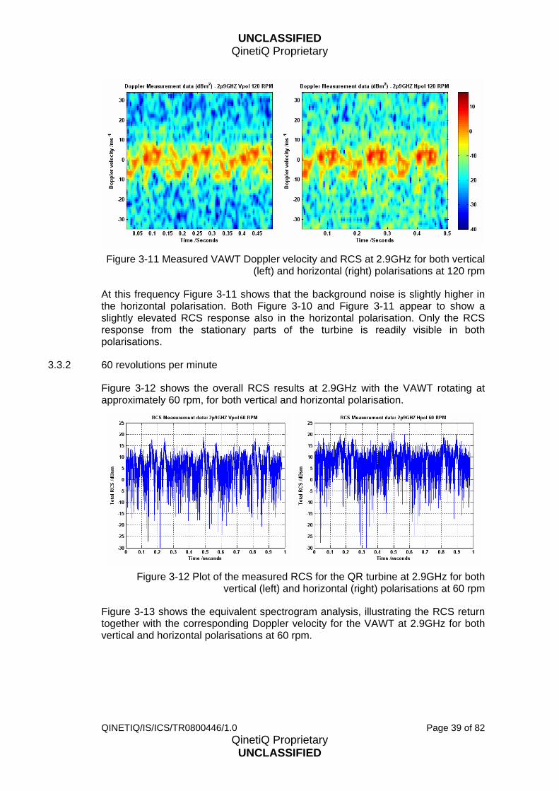
Figure 3-11 Measured VAWT Doppler velocity and RCS at 2.9GHz for both vertical (left) and horizontal (right) polarisations at 120 rpm
At this frequency Figure 3-11 shows that the background noise is slightly higher in the horizontal polarisation. Both Figure 3-10 and Figure 3-11 appear to show a slightly elevated RCS response also in the horizontal polarisation. Only the RCS response from the stationary parts of the turbine is readily visible in both polarisations.
3.3.2 60 revolutions per minute
Figure 3-12 shows the overall RCS results at 2.9GHz with the VAWT rotating at approximately 60 rpm, for both vertical and horizontal polarisation.
Figure 3-12 Plot of the measured RCS for the QR turbine at 2.9GHz for both vertical (left) and horizontal (right) polarisations at 60 rpm
Figure 3-13 shows the equivalent spectrogram analysis, illustrating the RCS return together with the corresponding Doppler velocity for the VAWT at 2.9GHz for both vertical and horizontal polarisations at 60 rpm.
UNCLASSIFIED QinetiQ Proprietary
QINETIQ/IS/ICS/TR0800446/1.0 Page 40 of 82 QinetiQ Proprietary
UNCLASSIFIED
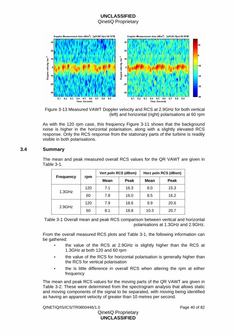
Figure 3-13 Measured VAWT Doppler velocity and RCS at 2.9GHz for both vertical (left) and horizontal (right) polarisations at 60 rpm
As with the 120 rpm case, this frequency Figure 3-11 shows that the background noise is higher in the horizontal polarisation, along with a slightly elevated RCS response. Only the RCS response from the stationary parts of the turbine is readily visible in both polarisations.
3.4 Summary
The mean and peak measured overall RCS values for the QR VAWT are given in Table 3-1.
Vert poln RCS (dBsm) Horz poln RCS (dBsm) Frequency rpm
Mean Peak Mean Peak
120 7.1 16.3 8.0 15.3 1.3GHz
60 7.8 16.0 8.5 16.2
120 7.9 18.6 9.9 20.6 2.9GHz
60 8.1 18.8 10.3 20.7
Table 3-1 Overall mean and peak RCS comparison between vertical and horizontal polarisations at 1.3GHz and 2.9GHz.
From the overall measured RCS plots and Table 3-1, the following information can be gathered:
• the value of the RCS at 2.9GHz is slightly higher than the RCS at 1.3GHz at both 120 and 60 rpm
• the value of the RCS for horizontal polarisation is generally higher than the RCS for vertical polarisation
• the is little difference in overall RCS when altering the rpm at either frequency
The mean and peak RCS values for the moving parts of the QR VAWT are given in Table 3-2. These were determined from the spectrogram analysis that allows static and moving components of the signal to be separated, with moving being identified as having an apparent velocity of greater than 10 metres per second.
UNCLASSIFIED QinetiQ Proprietary
QINETIQ/IS/ICS/TR0800446/1.0 Page 41 of 82 QinetiQ Proprietary
UNCLASSIFIED
Moving RCS (dBsm)
Vert poln RCS Horz poln RCS Frequency rpm
Mean Peak Mean Peak
120 -10.3 -5.5 -9.6 -4.9 1.3GHz
60 -13.1 -7.1 -13.2 -9.1
120 -3.5 1.1 -0.2 2.5 2.9GHz
60 -5.0 -1.6 -1.4 1.3
Table 3-2 Mean and peak RCS values comparison between vertical and horizontal polarisations at 1.3GHz and 2.9GHz for the moving parts of the turbine
From the measured spectrogram plots and Table 3-2, the following information can be gathered:
• the RCS contributions from the moving parts of the turbine at 2.9GHz is significantly higher than the RCS at 1.3GHz at both 120 and 60 rpm
• the RCS contributions from the moving parts of the turbine for horizontal polarisation is generally higher than the RCS for vertical polarisation
• the RCS contributions from the moving parts of the turbine is less at 60 rpm than 120 rpm at either frequency, although the effect is more pronounced at 1.3GHz
The RCS modelling results show that the overall RCS of the turbine is affected by the frequency and polarisation of the radar. The RCS contributions from the moving parts of the turbine are significantly lower than the overall RCS values.
Some of the conclusions for the measured RCS values may have been affected by the high levels of background noise, especially at 2.9GHz. This level of background noise also makes it difficult to resolve the outer blade structure in the Doppler spectra.
3.5 Modelled versus measurement
As stated in section 3.1, since the exact Funtington set up of the VAWT was not known at the time the modelling took place, two elevation angles were modelled, 0 and 1 degree. However, it was expected that the real elevation angle would be of the order of 1 degree. Once the set up of the VAWT at Funtington had been finalised, it was found that the real elevation angle was approximately 1.6 degrees. With the 1 degree PEC modelled data set being the closest match in elevation angle; this was used to compare with the measured data.
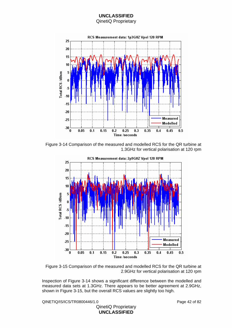
Figure 3-14 and Figure 3-15 compare the overall RCS curves for measured data and the 1 degree elevation angle PEC modelled data set, at 1.3GHz and 2.9GHz.
UNCLASSIFIED QinetiQ Proprietary
QINETIQ/IS/ICS/TR0800446/1.0 Page 42 of 82 QinetiQ Proprietary
UNCLASSIFIED
Figure 3-14 Comparison of the measured and modelled RCS for the QR turbine at 1.3GHz for vertical polarisation at 120 rpm
Figure 3-15 Comparison of the measured and modelled RCS for the QR turbine at 2.9GHz for vertical polarisation at 120 rpm
Inspection of Figure 3-14 shows a significant difference between the modelled and measured data sets at 1.3GHz. There appears to be better agreement at 2.9GHz, shown in Figure 3-15, but the overall RCS values are slightly too high.
UNCLASSIFIED QinetiQ Proprietary
QINETIQ/IS/ICS/TR0800446/1.0 Page 43 of 82 QinetiQ Proprietary
UNCLASSIFIED
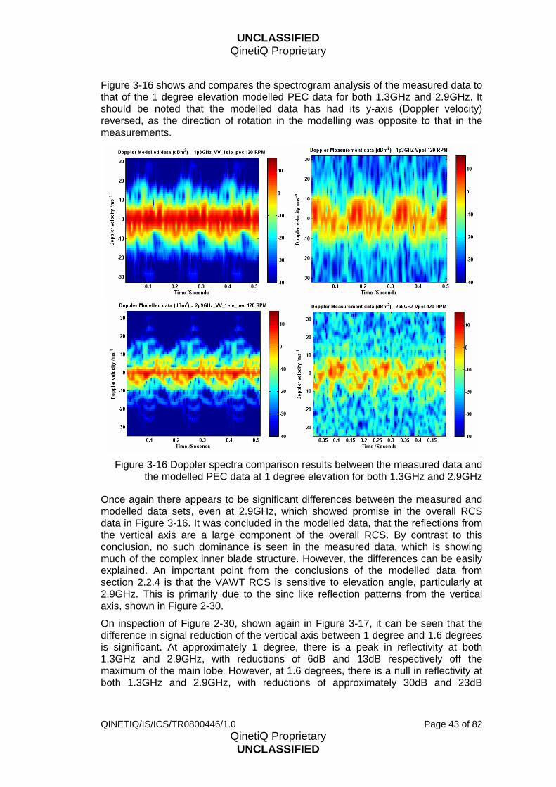
Figure 3-16 shows and compares the spectrogram analysis of the measured data to that of the 1 degree elevation modelled PEC data for both 1.3GHz and 2.9GHz. It should be noted that the modelled data has had its y-axis (Doppler velocity) reversed, as the direction of rotation in the modelling was opposite to that in the measurements.
Figure 3-16 Doppler spectra comparison results between the measured data and the modelled PEC data at 1 degree elevation for both 1.3GHz and 2.9GHz
Once again there appears to be significant differences between the measured and modelled data sets, even at 2.9GHz, which showed promise in the overall RCS data in Figure 3-16. It was concluded in the modelled data, that the reflections from the vertical axis are a large component of the overall RCS. By contrast to this conclusion, no such dominance is seen in the measured data, which is showing much of the complex inner blade structure. However, the differences can be easily explained. An important point from the conclusions of the modelled data from section 2.2.4 is that the VAWT RCS is sensitive to elevation angle, particularly at 2.9GHz. This is primarily due to the sinc like reflection patterns from the vertical axis, shown in Figure 2-30.
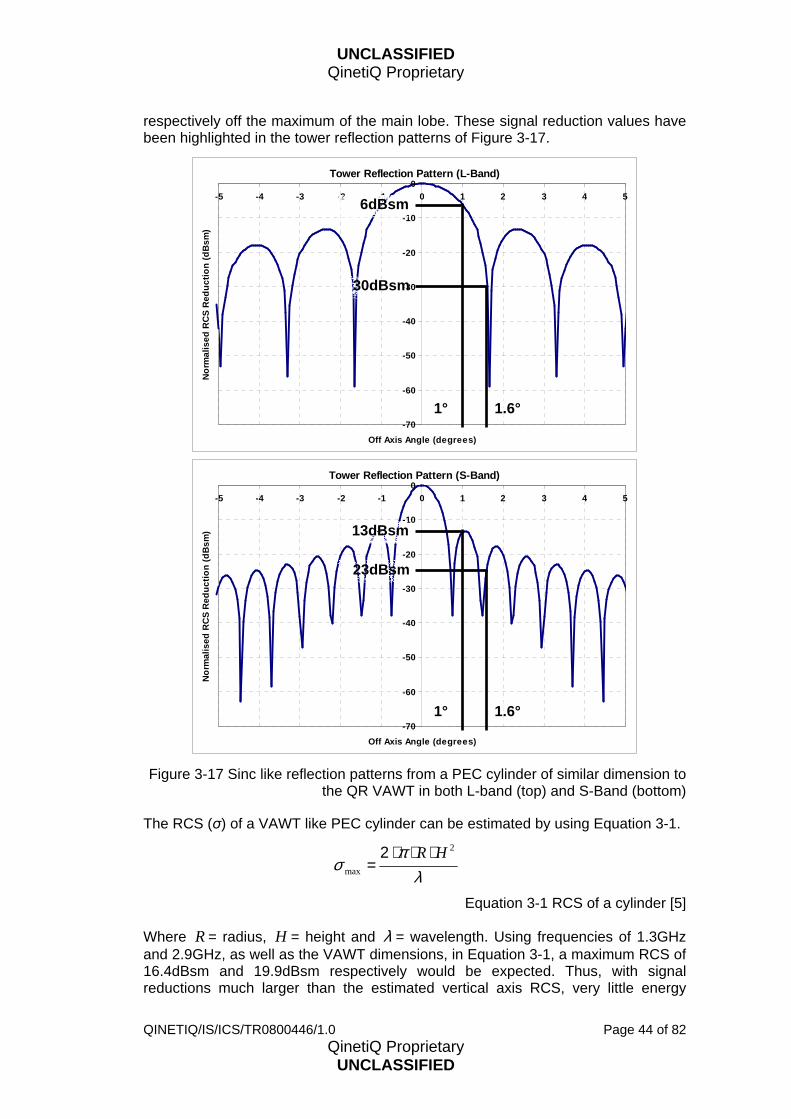
On inspection of Figure 2-30, shown again in Figure 3-17, it can be seen that the difference in signal reduction of the vertical axis between 1 degree and 1.6 degrees is significant. At approximately 1 degree, there is a peak in reflectivity at both 1.3GHz and 2.9GHz, with reductions of 6dB and 13dB respectively off the maximum of the main lobe. However, at 1.6 degrees, there is a null in reflectivity at both 1.3GHz and 2.9GHz, with reductions of approximately 30dB and 23dB
UNCLASSIFIED QinetiQ Proprietary
QINETIQ/IS/ICS/TR0800446/1.0 Page 44 of 82 QinetiQ Proprietary
UNCLASSIFIED
respectively off the maximum of the main lobe. These signal reduction values have been highlighted in the tower reflection patterns of Figure 3-17.
Tower Reflection Pattern (L-Band)
-70
-60
-50
-40
-30
-20
-10
0-5 -4 -3 -2 -1 0 1 2 3 4 5
Off Axis Angle (degrees)
Nor
mal
ised
RC
S R
educ
tion
(dB
sm)
Tower Reflection Pattern (S-Band)
-70
-60
-50
-40
-30
-20
-10
0-5 -4 -3 -2 -1 0 1 2 3 4 5
Off Axis Angle (degrees)
Nor
mal
ised
RC
S R
educ
tion
(dB
sm)
Figure 3-17 Sinc like reflection patterns from a PEC cylinder of similar dimension to the QR VAWT in both L-band (top) and S-Band (bottom)
The RCS (σ) of a VAWT like PEC cylinder can be estimated by using Equation 3-1.
λπ
σ2
max
HR ⋅⋅⋅=
2
Equation 3-1 RCS of a cylinder [5]
Where R = radius, H = height and λ = wavelength. Using frequencies of 1.3GHz and 2.9GHz, as well as the VAWT dimensions, in Equation 3-1, a maximum RCS of 16.4dBsm and 19.9dBsm respectively would be expected. Thus, with signal reductions much larger than the estimated vertical axis RCS, very little energy
1° 1.6°
30dBsm
6dBsm
1° 1.6°
23dBsm
13dBsm
UNCLASSIFIED QinetiQ Proprietary
QINETIQ/IS/ICS/TR0800446/1.0 Page 45 of 82 QinetiQ Proprietary
UNCLASSIFIED
would be expected to be reflected back from the vertical axis at this elevation angle. Hence, the measured data set would be more comparable to the RAM axis results at 1 degree elevation.
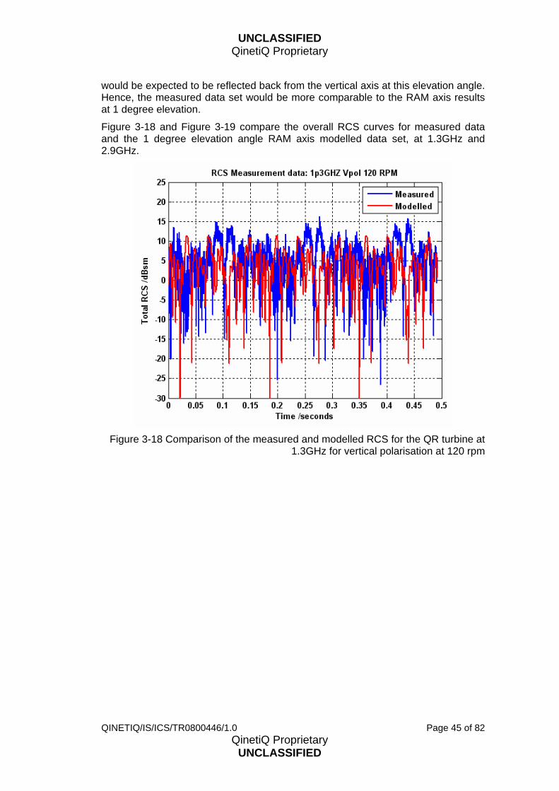
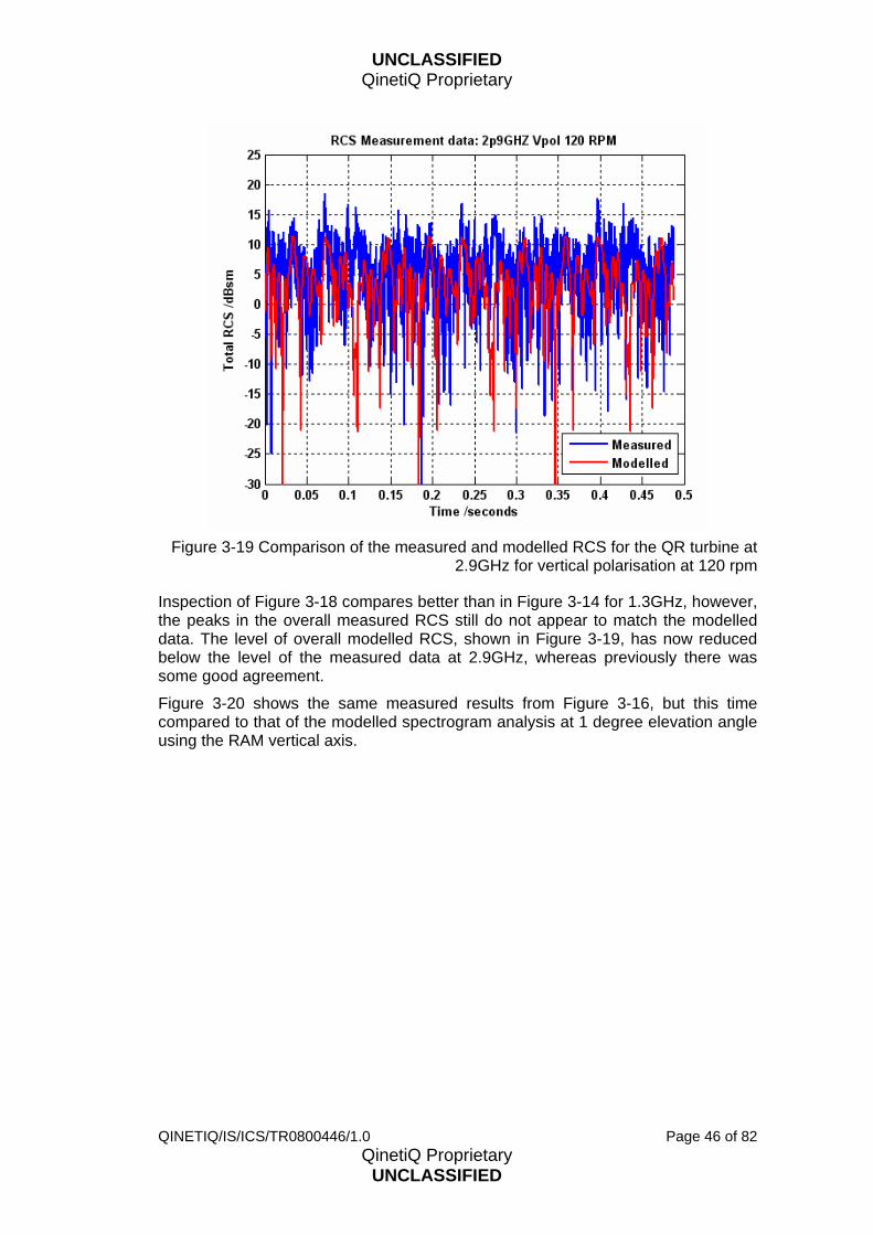
Figure 3-18 and Figure 3-19 compare the overall RCS curves for measured data and the 1 degree elevation angle RAM axis modelled data set, at 1.3GHz and 2.9GHz.
Figure 3-18 Comparison of the measured and modelled RCS for the QR turbine at 1.3GHz for vertical polarisation at 120 rpm
UNCLASSIFIED QinetiQ Proprietary
QINETIQ/IS/ICS/TR0800446/1.0 Page 46 of 82 QinetiQ Proprietary
UNCLASSIFIED
Figure 3-19 Comparison of the measured and modelled RCS for the QR turbine at 2.9GHz for vertical polarisation at 120 rpm
Inspection of Figure 3-18 compares better than in Figure 3-14 for 1.3GHz, however, the peaks in the overall measured RCS still do not appear to match the modelled data. The level of overall modelled RCS, shown in Figure 3-19, has now reduced below the level of the measured data at 2.9GHz, whereas previously there was some good agreement.
Figure 3-20 shows the same measured results from Figure 3-16, but this time compared to that of the modelled spectrogram analysis at 1 degree elevation angle using the RAM vertical axis.

UNCLASSIFIED QinetiQ Proprietary
QINETIQ/IS/ICS/TR0800446/1.0 Page 47 of 82 QinetiQ Proprietary
UNCLASSIFIED
Figure 3-20 Doppler spectra comparison results between the measured data and the modelled RAM axis data at 1 degree elevation for both 1.3GHz and 2.9GHz
There is now visibly much better agreement between the measured and modelled data sets at both 1.3GHz and 2.9GHz, and thus supporting the null tower reflection hypothesis. More of the fine blade structure in the central regions of the modelled spectra can be resolved due to the higher sampling rates achievable than in real measurements. The low reflectivity of the outer blade structure and higher levels of background noise make it difficult to compare the rest of the spectra. The RCS on the modelled data at 2.9GHz appears to be more one sided than in the real data.
The mean and peak RCS values for the QR VAWT are given in Table 3-3 whilst the mean and peak RCS contributions from the moving parts of the turbine are given in Table 3-4.
Measured RCS (dBsm) Modelled RCS (dBsm) Frequency
Mean Peak Mean Peak
1.3GHz 7.1 16.3 6.0 12.1
2.9GHz 7.9 18.6 5.4 11.5
Table 3-3 Overall mean and peak RCS comparison between measured and modelled data sets for both 1.3GHz and 2.9GHz
UNCLASSIFIED QinetiQ Proprietary
QINETIQ/IS/ICS/TR0800446/1.0 Page 48 of 82 QinetiQ Proprietary
UNCLASSIFIED
Moving RCS (dBsm)
Measured RCS Modelled RCS Frequency
Mean Peak Mean Peak
1.3GHz -10.3 -5.5 -12.4 -7.1
2.9GHz -3.5 1.1 -15.1 -8.1
Table 3-4 Mean and peak RCS values comparison between the measured and modelled data sets at 1.3GHz and 2.9GHz for the moving parts of the turbine
Tables 3-3 and 3-4 support the conclusions that there is general agreement between measured and modelled data, particularly with the moving RCS at 1.3GHz. However, it can be seen that on average, the measured RCS values are higher than in the modelled data. It is also apparent that the higher levels of background noise may be affecting results of the measured RCS at 2.9GHz.
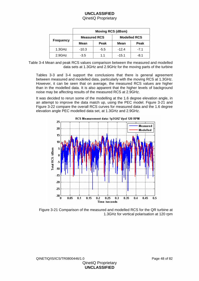
It was decided to rerun some of the modelling at the 1.6 degree elevation angle, in an attempt to improve the data match up, using the PEC model. Figure 3-21 and Figure 3-22 compare the overall RCS curves for measured data and the 1.6 degree elevation angle PEC modelled data set, at 1.3GHz and 2.9GHz.
Figure 3-21 Comparison of the measured and modelled RCS for the QR turbine at 1.3GHz for vertical polarisation at 120 rpm
UNCLASSIFIED QinetiQ Proprietary
QINETIQ/IS/ICS/TR0800446/1.0 Page 49 of 82 QinetiQ Proprietary
UNCLASSIFIED
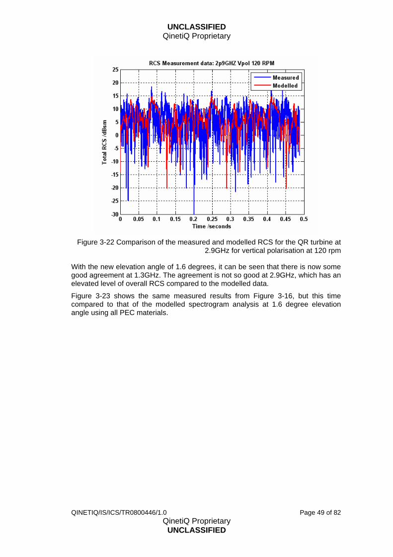
Figure 3-22 Comparison of the measured and modelled RCS for the QR turbine at 2.9GHz for vertical polarisation at 120 rpm
With the new elevation angle of 1.6 degrees, it can be seen that there is now some good agreement at 1.3GHz. The agreement is not so good at 2.9GHz, which has an elevated level of overall RCS compared to the modelled data.
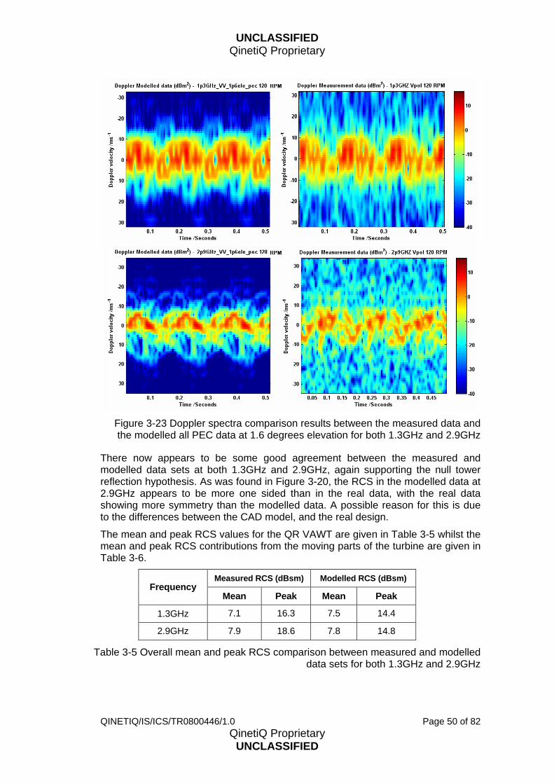
Figure 3-23 shows the same measured results from Figure 3-16, but this time compared to that of the modelled spectrogram analysis at 1.6 degree elevation angle using all PEC materials.
UNCLASSIFIED QinetiQ Proprietary
QINETIQ/IS/ICS/TR0800446/1.0 Page 50 of 82 QinetiQ Proprietary
UNCLASSIFIED
Figure 3-23 Doppler spectra comparison results between the measured data and the modelled all PEC data at 1.6 degrees elevation for both 1.3GHz and 2.9GHz
There now appears to be some good agreement between the measured and modelled data sets at both 1.3GHz and 2.9GHz, again supporting the null tower reflection hypothesis. As was found in Figure 3-20, the RCS in the modelled data at 2.9GHz appears to be more one sided than in the real data, with the real data showing more symmetry than the modelled data. A possible reason for this is due to the differences between the CAD model, and the real design.
The mean and peak RCS values for the QR VAWT are given in Table 3-5 whilst the mean and peak RCS contributions from the moving parts of the turbine are given in Table 3-6.
Measured RCS (dBsm) Modelled RCS (dBsm) Frequency
Mean Peak Mean Peak
1.3GHz 7.1 16.3 7.5 14.4
2.9GHz 7.9 18.6 7.8 14.8
Table 3-5 Overall mean and peak RCS comparison between measured and modelled data sets for both 1.3GHz and 2.9GHz
UNCLASSIFIED QinetiQ Proprietary
QINETIQ/IS/ICS/TR0800446/1.0 Page 51 of 82 QinetiQ Proprietary
UNCLASSIFIED
Moving RCS (dBsm)
Measured RCS Modelled RCS Frequency
Mean Peak Mean Peak
1.3GHz -10.3 -5.5 -12.2 -6.4
2.9GHz -3.5 1.1 -13.6 -6.4
Table 3-6 Mean and peak RCS values comparison between the measured and modelled data sets at 1.3GHz and 2.9GHz for the moving parts of the turbine
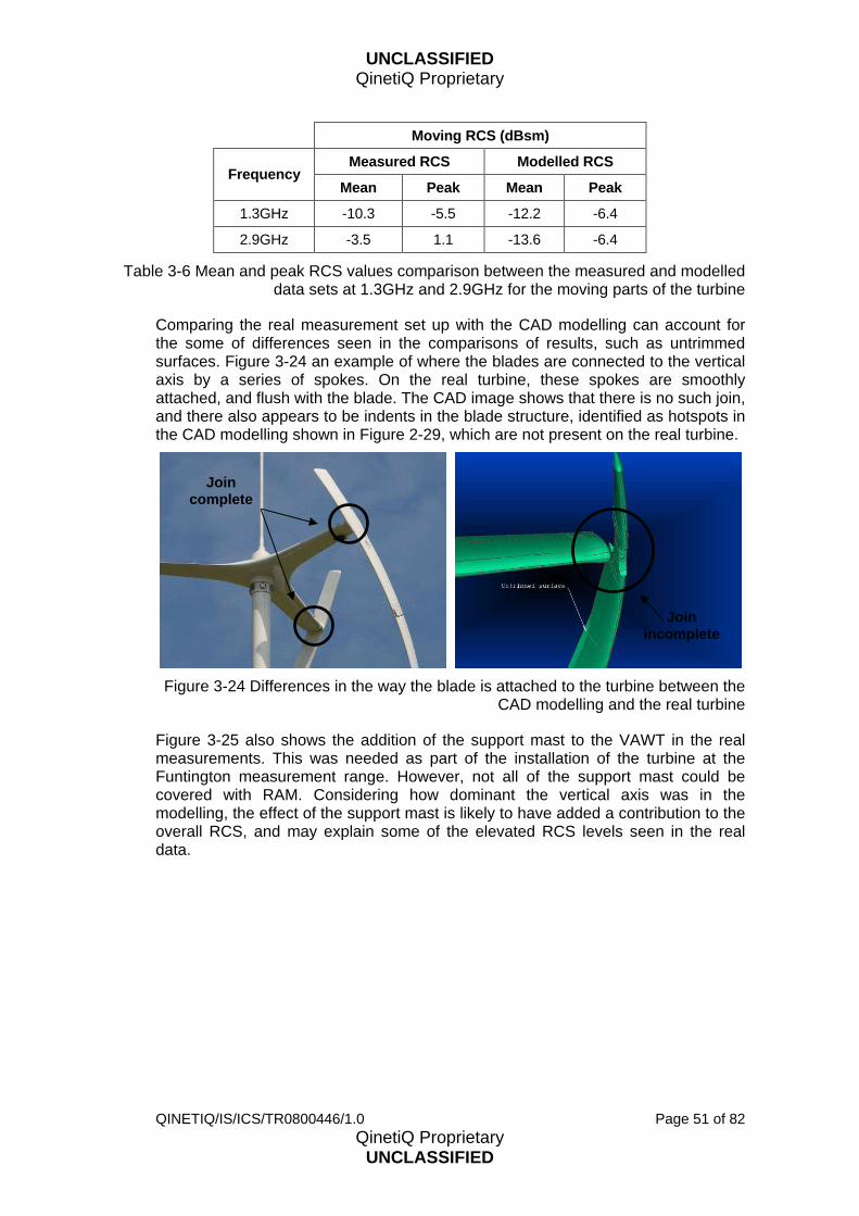
Comparing the real measurement set up with the CAD modelling can account for the some of differences seen in the comparisons of results, such as untrimmed surfaces. Figure 3-24 an example of where the blades are connected to the vertical axis by a series of spokes. On the real turbine, these spokes are smoothly attached, and flush with the blade. The CAD image shows that there is no such join, and there also appears to be indents in the blade structure, identified as hotspots in the CAD modelling shown in Figure 2-29, which are not present on the real turbine.
Figure 3-24 Differences in the way the blade is attached to the turbine between the CAD modelling and the real turbine
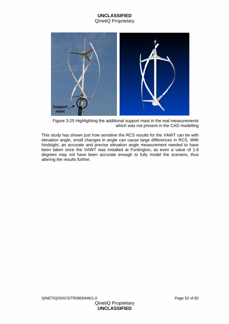
Figure 3-25 also shows the addition of the support mast to the VAWT in the real measurements. This was needed as part of the installation of the turbine at the Funtington measurement range. However, not all of the support mast could be covered with RAM. Considering how dominant the vertical axis was in the modelling, the effect of the support mast is likely to have added a contribution to the overall RCS, and may explain some of the elevated RCS levels seen in the real data.
Join complete
Join incomplete
UNCLASSIFIED QinetiQ Proprietary
QINETIQ/IS/ICS/TR0800446/1.0 Page 52 of 82 QinetiQ Proprietary
UNCLASSIFIED
Figure 3-25 Highlighting the additional support mast in the real measurements which was not present in the CAD modelling
This study has shown just how sensitive the RCS results for the VAWT can be with elevation angle, small changes in angle can cause large differences in RCS. With hindsight, an accurate and precise elevation angle measurement needed to have been taken once the VAWT was installed at Funtington, as even a value of 1.6 degrees may not have been accurate enough to fully model the scenario, thus altering the results further.
Support mast
UNCLASSIFIED QinetiQ Proprietary
QINETIQ/IS/ICS/TR0800446/1.0 Page 53 of 82 QinetiQ Proprietary
UNCLASSIFIED
4 Assessment of the Impact of a Vertical Axis Wind Turbine This section of the report looks at the potential impact that the VAWT could have on radar, by using the measurement results from section 3 and assessing its detectability for a typical S-Band air traffic control radar. This section uses the same methods used in the previous QinetiQ report, which evaluated the impact of micro turbines on radar [6], and should be read in conjunction with this section. Therefore, only a brief outline of the method used is presented here.
To assess the detectability of the VAWT, the minimum detectable RCS for a specified radar needs to be calculated. The naval electromagnetic environment simulation suite (NEMESiS) radar propagation tool can be used to calculate the minimum detectable RCS in a free space6 environment. NEMESiS has been developed by QinetiQ over the past decade to model the influence of the environment on military radar systems for the Ministry of Defence (MoD). At the heart of the model is an advanced propagation algorithm that simulates how microwave energy propagates through the atmosphere, reflects off the earth’s surface and diffracts over terrain.
The specific radar being considered in this example impact study is a standard Watchman S-Band radar, with no antenna tilt, no terrain and no sensitivity time control (STC) applied, which is designed to reduce the effects of clutter on a radar system.
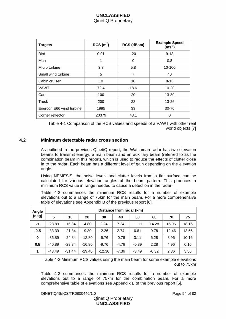
4.1 Comparison with other targets
Using the results from the measurements taken of the VAWT in section 3, a comparison can be made to put the RCS values of a VAWT in context. Table 4-1 shows the RCS and example speeds of a number of real world objects, and compares them to that of the VAWT.
From Table 4-1, its can be seen that the effects of a car or truck are likely to be comparable to that of a VAWT, and would be more widely spread out in the urban and rural areas than a VAWT.
6 Free space means that there is no material or other physical phenomenon present except the phenomenon under consideration; in this case no terrain or the effects multipath is included in the analysis.
UNCLASSIFIED QinetiQ Proprietary
QINETIQ/IS/ICS/TR0800446/1.0 Page 54 of 82 QinetiQ Proprietary
UNCLASSIFIED
Targets RCS (m 2) RCS (dBsm) Example Speed (ms -1)
Bird 0.01 -20 9-13
Man 1 0 0.8
Micro turbine 3.8 5.8 10-100
Small wind turbine 5 7 40
Cabin cruiser 10 10 8-13
VAWT 72.4 18.6 10-20
Car 100 20 13-30
Truck 200 23 13-26
Enercon E66 wind turbine 1995 33 30-70
Corner reflector 20379 43.1 0
Table 4-1 Comparison of the RCS values and speeds of a VAWT with other real world objects [7]
4.2 Minimum detectable radar cross section
As outlined in the previous QinetiQ report, the Watchman radar has two elevation beams to transmit energy, a main beam and an auxiliary beam (referred to as the combination beam in this report), which is used to reduce the effects of clutter close in to the radar. Each beam has a different level of gain depending on the elevation angle.
Using NEMESiS, the noise levels and clutter levels from a flat surface can be calculated for various elevation angles of the beam pattern. This produces a minimum RCS value in range needed to cause a detection in the radar.
Table 4-2 summarises the minimum RCS results for a number of example elevations out to a range of 75km for the main beam. For a more comprehensive table of elevations see Appendix B of the previous report [6].
Distance from radar (km) Angle (deg) 5 10 20 30 40 50 60 70 75
-1 -28.89 -16.84 -4.80 2.24 7.24 11.11 14.28 16.96 18.16
-0.5 -33.39 -21.34 -9.30 -2.26 2.74 6.61 9.78 12.46 13.66
0 -36.89 -24.84 -12.80 -5.76 -0.76 3.11 6.28 8.96 10.16
0.5 -40.89 -28.84 -16.80 -9.76 -4.76 -0.89 2.28 4.96 6.16
1 -43.49 -31.44 -19.40 -12.36 -7.36 -3.49 -0.32 2.36 3.56
Table 4-2 Minimum RCS values using the main beam for some example elevations out to 75km
Table 4-3 summarises the minimum RCS results for a number of example elevations out to a range of 75km for the combination beam. For a more comprehensive table of elevations see Appendix B of the previous report [6].
UNCLASSIFIED QinetiQ Proprietary
QINETIQ/IS/ICS/TR0800446/1.0 Page 55 of 82 QinetiQ Proprietary
UNCLASSIFIED
Distance from radar (km) Angle (deg) 5 10 20 30 40 50 60 70 75
-1 -18.39 -6.34 5.70 12.74 17.74 21.61 24.78 27.46 28.66
-0.5 -21.94 -9.89 2.15 9.19 14.19 18.06 21.23 23.91 25.11
0 -24.89 -12.84 -0.80 6.24 11.24 15.11 18.28 20.96 22.16
0.5 -28.39 -16.34 -4.30 2.74 7.74 11.61 14.78 17.46 18.66
1 -31.29 -19.24 -7.20 -0.16 4.84 8.71 11.88 14.56 15.76
Table 4-3 Minimum RCS values using the combination beam for all elevations out to 75km
The above minimum RCS values give an indication of when certain objects will become visible to the radar. Using the RCS values determined for the VAWT in section 3, the detection ranges can be deduced.
4.3 Range a vertical axis wind turbine become visib le
The equation to determine the range at which an object become visible is given in Equation 4-1.
( )
41
3
2
4
=
reflections
rtt
PL
GGPR
πσλ
Equation 4-1 Radar range equation
Where the symbols have the following meanings:
Pt Transmitter power (Watts)
Gt Transmitter gain
Gr Receiver gain
σ VAWT RCS (monostatic) (m2)
λ Wavelength (m)
R Range of turbine from radar (m)
L System losses
Using the Watchman radar parameters given in the previous QinetiQ report, the detection ranges for the VAWT can be found when the received power (Preflection) is equal to, or greater than, the sensitivity of the radar.
Table 4-4 shows the detection ranges for the maximum static component RCS (18.6dB) of the VAWT for a number of different elevations using both the main and combination beams. The peak RCS of the static component has been used rather than the mean to illustrate the worst case.
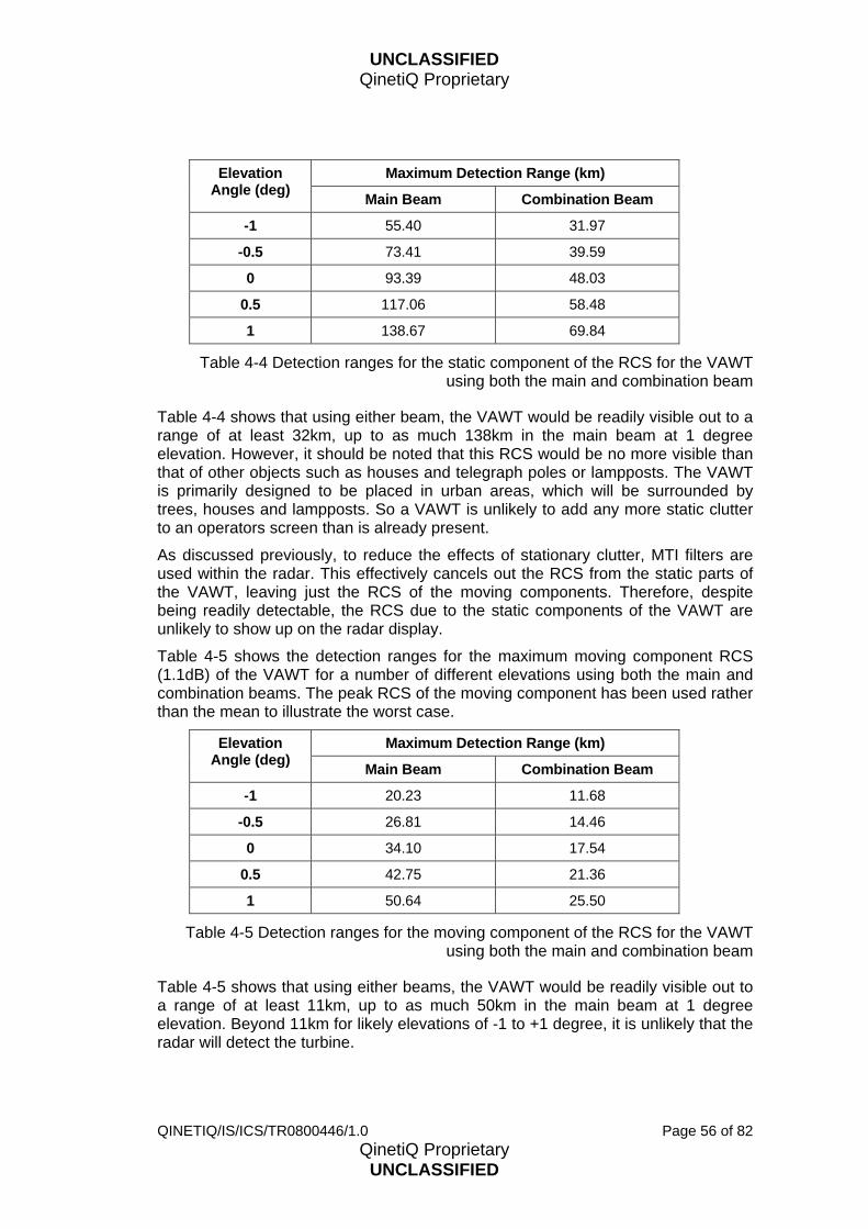
UNCLASSIFIED QinetiQ Proprietary
QINETIQ/IS/ICS/TR0800446/1.0 Page 56 of 82 QinetiQ Proprietary
UNCLASSIFIED
Maximum Detection Range (km) Elevation Angle (deg)
Main Beam Combination Beam
-1 55.40 31.97
-0.5 73.41 39.59
0 93.39 48.03
0.5 117.06 58.48
1 138.67 69.84
Table 4-4 Detection ranges for the static component of the RCS for the VAWT using both the main and combination beam
Table 4-4 shows that using either beam, the VAWT would be readily visible out to a range of at least 32km, up to as much 138km in the main beam at 1 degree elevation. However, it should be noted that this RCS would be no more visible than that of other objects such as houses and telegraph poles or lampposts. The VAWT is primarily designed to be placed in urban areas, which will be surrounded by trees, houses and lampposts. So a VAWT is unlikely to add any more static clutter to an operators screen than is already present.
As discussed previously, to reduce the effects of stationary clutter, MTI filters are used within the radar. This effectively cancels out the RCS from the static parts of the VAWT, leaving just the RCS of the moving components. Therefore, despite being readily detectable, the RCS due to the static components of the VAWT are unlikely to show up on the radar display.
Table 4-5 shows the detection ranges for the maximum moving component RCS (1.1dB) of the VAWT for a number of different elevations using both the main and combination beams. The peak RCS of the moving component has been used rather than the mean to illustrate the worst case.
Maximum Detection Range (km) Elevation Angle (deg)
Main Beam Combination Beam
-1 20.23 11.68
-0.5 26.81 14.46
0 34.10 17.54
0.5 42.75 21.36
1 50.64 25.50
Table 4-5 Detection ranges for the moving component of the RCS for the VAWT using both the main and combination beam
Table 4-5 shows that using either beams, the VAWT would be readily visible out to a range of at least 11km, up to as much 50km in the main beam at 1 degree elevation. Beyond 11km for likely elevations of -1 to +1 degree, it is unlikely that the radar will detect the turbine.
UNCLASSIFIED QinetiQ Proprietary
QINETIQ/IS/ICS/TR0800446/1.0 Page 57 of 82 QinetiQ Proprietary
UNCLASSIFIED
4.4 Cumulative effect on detection range
This sub-section looks at the cumulative effect that a number of possible VAWTs may have on the detection ranges.
The resolution of a radar is the minimum separation between two targets that permits them to be distinguished. The size of a resolution cell depends on the pulse length (defines the downrange resolution) and the beamwidth (affects the cross-range resolution) of the radar. This creates a resolution cell whereby targets cannot be resolved and appear to be merged into a single target on a radar display.
The Watchman radar has a beam width of 1.5 degrees and a pulse length 0.8µs (see previous report for more detailed parameters [6]). The radar resolution cell sizes have been calculated for a number of different ranges and a few examples are given in the following figures.
Figure 4-1 shows a resolution cell for the Watchman radar at 5km plotted in Google Earth. It also shows the approximate number of houses that could fit into a cell of this size at the specified range, which equates to approximately 24. Assuming each house has one turbine installed, there could potentially be 24 turbines in a single resolution cell at a range of 5km.
Figure 4-1Watchman resolution cell at 5km plotted in Google Earth, and zoomed in (right) to highlight the number of houses in encompasses
Figure 4-2 shows a resolution cell for the Watchman radar at 40km plotted in Google Earth. Scaling up the number of houses that fit into a cell at 5km, the number of houses that could fit into a cell at 40km would be approximately 192. Assuming each house has one turbine installed, there could potentially be 192 turbines in a single resolution cell at a range of 40km.
UNCLASSIFIED QinetiQ Proprietary
QINETIQ/IS/ICS/TR0800446/1.0 Page 58 of 82 QinetiQ Proprietary
UNCLASSIFIED
Figure 4-2 Watchman resolution cell at 40km plotted in Google Earth
Figure 4-3 shows a resolution cell for the Watchman radar at 75km plotted in Google Earth. Scaling up the number of houses that fit into a cell at 5km, the number of houses that could fit into a cell at 75km would be approximately 360. Assuming each house has one turbine installed, there could potentially be 360 turbines in a single resolution cell at a range of 75km.
Figure 4-3 Watchman resolution cell at 75km plotted in Google Earth
Table 4-6 shows the cell sizes and the number of turbines that the cell encompasses for a number of different ranges from the radar. The table also shows the apparent RCS that would be seen by adding up the RCS components from each of the VAWTs that would be encompassed by the resolution cell. This is taken as a worst case scenario, in reality the phases of the VAWT signal would not add coherently, thus giving a lower overall RCS value.
UNCLASSIFIED QinetiQ Proprietary
QINETIQ/IS/ICS/TR0800446/1.0 Page 59 of 82 QinetiQ Proprietary
UNCLASSIFIED
Distance (km)
Width (m) No. Turbines
Max RCS from moving
component
Max RCS from static
component
5 131 24 14.90 32.40
10 262 48 17.91 35.41
20 524 96 20.92 38.42
30 785 144 22.68 40.18
40 1047 192 23.93 41.43
50 1309 240 24.90 42.40
60 1571 288 25.69 43.19
70 1833 336 26.36 43.86
75 1964 360 26.66 44.16
Table 4-6 Cumulative RCS values for the static and moving components of a VAWT with range
Table 4-6 shows that as the resolution cell width increases in range, the moving and static component RCS also increase. However, due to the nature of the logarithmic value, the RCS does not scale linearly, and plateaus. This means that as range increases, it takes many more VAWTs to significantly increase the RCS.
Table 4-7 shows the number of VAWTs it would take in a resolution cell to reach the minimum detectable RCS at various ranges for different elevation angles.
Distance from radar (km) Angle (deg) 5 10 20 30 40 50 60 70 75
-1 1 1 3 15 47 113 234 433 571
-0.5 1 1 2 7 21 50 104 191 252
0 1 1 1 4 11 26 53 97 128
0.5 1 1 1 2 5 12 24 44 58
1 1 1 1 1 3 6 12 23 30
Max likely
24 48 96 144 192 240 288 336 360
Table 4-7 Numbers of turbines needed to reach the minimum detectable RCS using the combination beam compared to that of the maximum likely number of turbines
in a resolution cell at a given range
It is apparent from Table 4-7 that as the distance from the radar increases, the number of turbines needed to create a detection in free space also increases. At longer ranges, and low elevation angles, the numbers of turbines needed begins to exceed realistic values.
With many turbines in a single range cell, as discussed before, they will all appear to be a single target. This means that as well as the RCS adding up, the MTI signal, or more accurately the phase of each of the turbines, will add up too. As mentioned before, each of the turbines are unlikely to add coherently, creating a chaotic phase
UNCLASSIFIED QinetiQ Proprietary
QINETIQ/IS/ICS/TR0800446/1.0 Page 60 of 82 QinetiQ Proprietary
UNCLASSIFIED
return. This would make it appear more like a static component, thus making it easier for the radar to cancel the return when using MTI filters.
4.5 Impact summary
In summary, at certain elevation angles, the radar has the potential to see the static component of a VAWT out to a range of 32-138km. However, these detection ranges have been calculated in a free space environment without terrain clutter or multipath effects. The static clutter created by the VAWT would be set amongst other real world objects such as houses or lampposts, typical of an urban area
Typical land clutter RCS values can be taken from the Billingsley land clutter model, and compared to the cumulative VAWT RCS values. Billingsley uses a clutter power of approximately -30dBsm/m2 to -20dBsm/m2 for an S-Band radar [8]. Thus, for a resolution cell at 5km from the radar this gives a clutter background level of approximately 9dBsm to 24dBsm, which would be enough to cause a detection, therefore, adding the clutter power of a VAWT would have little additional affect.
At certain elevation angles, the radar has the potential to see the moving component of the turbine out to a range of approximately 51km. Again, urban clutter attributed to cars and trucks, which have a comparable RCS return, would create similar clutter levels already. Therefore, the addition of a VAWT to this clutter would add have limited impact.
The cumulative analysis showed that as the range increased, the number of turbines needed to reach the minimum detectable RCS at longer ranges and low elevation angles reach unrealistic numbers to fit within a resolution cell. Moreover, with the VAWT being integrated into building designs, and placed on roof tops, there is likely to be a high amount of obscuration within the urban environment, thus potentially obscuring, or limiting the impact of the VAWT in terms of radar detection.
Therefore, taking into account the use of a radar’s MTI filters, the likely clutter levels and obscuration associated with the urban environment, it is highly unlikely that a VAWT will add any additional clutter levels to that already detected and dealt with by a radar.
UNCLASSIFIED QinetiQ Proprietary
QINETIQ/IS/ICS/TR0800446/1.0 Page 61 of 82 QinetiQ Proprietary
UNCLASSIFIED
5 Conclusions QinetiQ was contracted by the ADATS IPT to predict and measure the RCS of a VAWT, as well as assess the potential impact it would have on radar. The VAWT used for the study was the QR qr5, a 7kW turbine that is roughly 5 metres high and 3 metres in width.
To predict the RCS of the VAWT, a CAD model was created, with a finite element mesh applied to it. The RCS predictions were calculated using the QinetiQ RCS prediction tool, Spectre®. The configuration tool was set up to run at frequencies of 1.3GHz and 2.9GHz, to represent L-Band and S-Band radars, at elevation angles of 0 and 1 degrees for a PEC material turbine assembly in free space.
It was found that the mean and peak modelled RCS values for the QR VAWT ranged from 10.0dBsm to 17.7dBsm and 16.3dBsm to 20.5dBsm respectively, depending on both the frequency of the radar and the elevation angle. The analysis showed that the dominant source of RCS was the central vertical axis of the VAWT, which masked some of the reflections from the blades.
The RCS predictions were repeated with a RAM applied to the vertical axis, thus allowing more reflections from the blades to be analysed. The results when using RAM on the axis showed that the mean and peak modelled RCS values of the turbine ranged from 4.4dBsm to 6.0dBsm and 10.9dBsm to 11.5dBsm respectively, depending on both the frequency of the radar and the elevation angle.
A spectrogram analysis was carried out, allowing Doppler velocity information to be extracted from the RCS data. Identifying the RCS of the moving components is important since many types of radar in the United Kingdom use filters to remove signals from static, or slow moving, objects. Therefore, it is the RCS from the moving parts of the turbine, with speeds roughly greater than 10 metres per second, that is likely to have the greatest impact on radar.
The mean and peak RCS values for the moving components of the QR VAWT ranged from -15.0dBsm to -11.1dBsm and -8.3dBsm to -4.8dBsm respectively. The RAM axis results showed that the mean and peak RCS for the moving components of the turbine ranged from -15.2dBsm to -11.5dBsm and -8.4dBsm to -5.4dBsm respectively.
A real radar measurement trial was also undertaken by installing a QR qr5 VAWT at the QinetiQ Funtington measurement range on the south coast of England. The final set up of the turbine meant that the radar elevation angle with respect to the turbine was 1.6 degrees, slightly more than was originally modelled with Spectre. Measurements were taken at both 1.3GHz and 2.9GHz using vertical and horizontal polarisations.
The mean and peak measured RCS values for the QR VAWT using vertical polarisation ranged from 7.1dBsm to 8.1dBsm and 16.3dBsm to 18.8dBsm respectively. The mean and peak measured RCS values for the QR VAWT using horizontal polarisation ranged from 8.0dBsm to 10.3dBsm and 15.3dBsm to 20.7dBsm respectively.
A spectrogram analysis showed the mean and peak RCS for the moving parts of the QR VAWT, using vertical polarisation, ranged from -13.1dBsm to -3.5dBsm and -7.1dBsm to 1.1dBsm respectively. The mean and peak RCS for the moving parts
UNCLASSIFIED QinetiQ Proprietary
QINETIQ/IS/ICS/TR0800446/1.0 Page 62 of 82 QinetiQ Proprietary
UNCLASSIFIED
of the turbine, using horizontal polarisation, ranged from -13.2dBsm to -0.2dBsm and -9.1dBsm to 2.5dBsm respectively.
Comparing the measured data to that of the modelled data showed some good agreement when using the 1 degree elevation RAM axis data set. It was decided to run additional Spectre modelling to assess the RCS of the VAWT at 1.6 degrees. Comparing these additional results yielded better agreement between the modelled and measured data sets. It was found that the RCS of the VAWT was extremely sensitive to elevation angle, particularly at 2.9GHz. At 1.6 degrees elevation angle there appeared to be minimal reflection from the vertical axis of the VAWT, which was the dominant feature at 0 and 1 degrees, and explains why the RAM modelled data compared better against the real data than the PEC modelling.
Further analysis showed that overall, the measured data seemed to be slightly higher in RCS than the modelled data, but the high level of background noise in the real measurements made it difficult to pick out some of the blade structure in the Doppler spectra. When comparing images of the real VAWT installed at Funtington to that of the CAD used in the modelling, differences were found which were likely to account for the differences when comparing the data.
The last part of this study examined the detection ranges and cumulative effects for a VAWT. At certain elevation angles, the radar has the potential to see the static component of the turbine out to a range of 32-138km. However, these detection ranges have been calculated in a free space environment without terrain clutter or multipath effects. The static clutter created by the VAWT would be set amongst other real world objects such as houses or lampposts, typical of an urban area
At certain elevation angles, the radar has the potential to see the moving component of the turbine out to a range of approximately 51km. Again, urban clutter attributed to cars and trucks, which have a comparable RCS return, would have already created similar clutter levels. Therefore, the addition of a VAWT to this clutter would add have limited impact.
However, taking into account the use of MTI filters in radar, and the likely clutter levels and obscuration associated with the urban environment, it is highly unlikely that a VAWT will add any additional clutter levels to that of what is already seen and dealt with by a radar.
UNCLASSIFIED QinetiQ Proprietary
QINETIQ/IS/ICS/TR0800446/1.0 Page 63 of 82 QinetiQ Proprietary
UNCLASSIFIED
6 References [1] quietrevolution, URL: http://www.quietrevolution.co.uk/qr5.htm, June 2008 [2] BWEA, URL: http://www.bwea.com/small/planning.html, June 2008 [3] Wood, A. quietrevolution ltd, QinetiQ qr5 modelling, e-mail to Dearman, S.
QinetiQ IS Division. Available e-mail: [email protected], 1st May 2008
[4] Hill, K., Zelinski, G., Van, T. and Vogel, C. Computational Electromagnetics (CEM) Prediction of a Windmill – Briefing to NATO Sensors Group,US Air Force Research Laboratory & ATK Space Systems Inc.11th June 2007
[5] Aerospaceweb.org, URL: http://www.aerospaceweb.org/question/electronics/q0168.shtml, June 2008
[6] New, C., Moldau, S. Assessment of wind turbine effects for DCSA, QinetiQ, QINETIQ/D&TS/SEA/TA0705054/1.0, March 2007
[7] Cristian Wolff, Radar Basics, URL: http://www.radartutorial.eu/18.explanations/ex09.en.html, June 2008
[8] Billingsley, J.B. Low Angle Radar Land Clutter, (SciTech Publishing Inc, USA), 2005
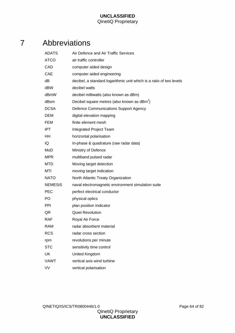
UNCLASSIFIED QinetiQ Proprietary
QINETIQ/IS/ICS/TR0800446/1.0 Page 64 of 82 QinetiQ Proprietary
UNCLASSIFIED
7 Abbreviations ADATS Air Defence and Air Traffic Services
ATCO air traffic controller
CAD computer aided design
CAE computer aided engineering
dB decibel, a standard logarithmic unit which is a ratio of two levels
dBW decibel watts
dBmW decibel milliwatts (also known as dBm)
dBsm Decibel square metres (also known as dBm2)
DCSA Defence Communications Support Agency
DEM digital elevation mapping
FEM finite element mesh
IPT Integrated Project Team
HH horizontal polarisation
IQ In-phase & quadrature (raw radar data)
MoD Ministry of Defence
MPR multiband pulsed radar
MTD Moving target detection
MTI moving target indication
NATO North Atlantic Treaty Organization
NEMESiS naval electromagnetic environment simulation suite
PEC perfect electrical conductor
PO physical optics
PPI plan position Indicator
QR Quiet Revolution
RAF Royal Air Force
RAM radar absorbent material
RCS radar cross section
rpm revolutions per minute
STC sensitivity time control
UK United Kingdom
VAWT vertical axis wind turbine
VV vertical polarisation
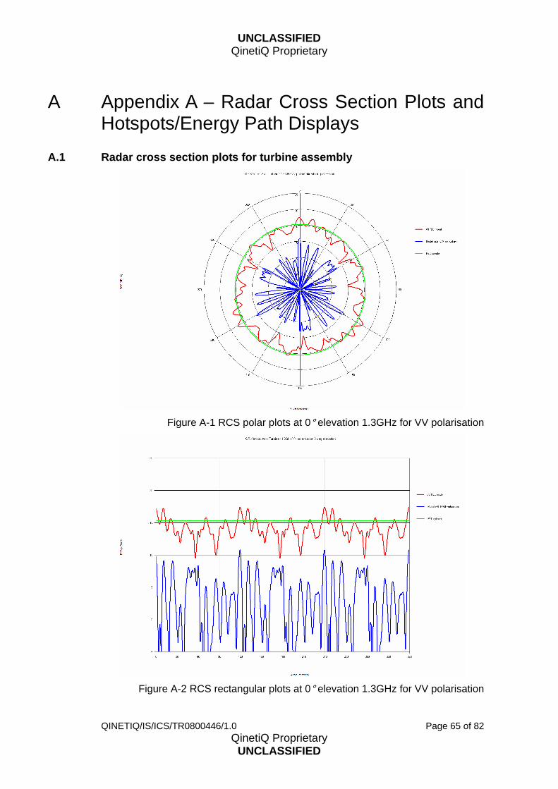
UNCLASSIFIED QinetiQ Proprietary
QINETIQ/IS/ICS/TR0800446/1.0 Page 65 of 82 QinetiQ Proprietary
UNCLASSIFIED
A Appendix A – Radar Cross Section Plots and Hotspots/Energy Path Displays
A.1 Radar cross section plots for turbine assembly
Figure A-1 RCS polar plots at 0° elevation 1.3GHz for VV polarisation
Figure A-2 RCS rectangular plots at 0° elevation 1.3GHz for VV polarisation
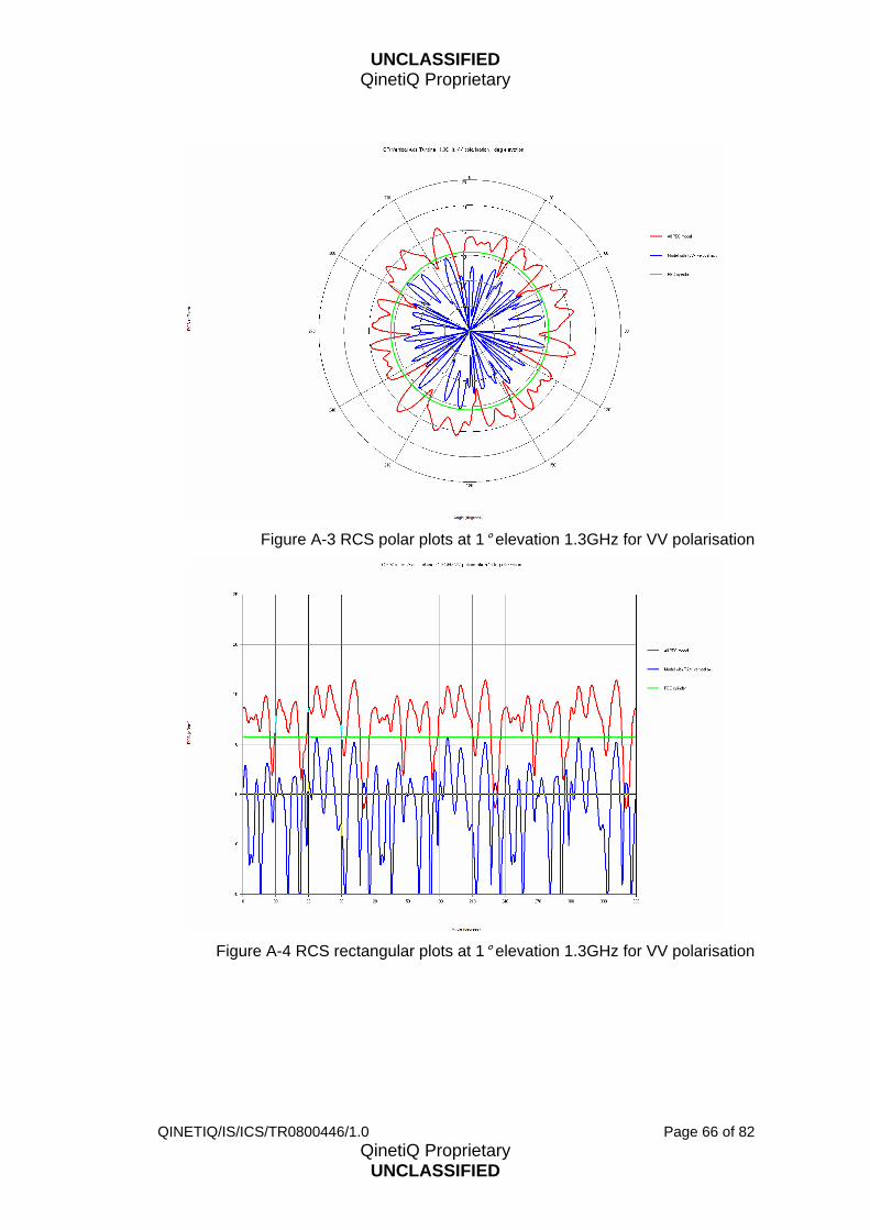
UNCLASSIFIED QinetiQ Proprietary
QINETIQ/IS/ICS/TR0800446/1.0 Page 66 of 82 QinetiQ Proprietary
UNCLASSIFIED
Figure A-3 RCS polar plots at 1° elevation 1.3GHz for VV polarisation
Figure A-4 RCS rectangular plots at 1° elevation 1.3GHz for VV polarisation
UNCLASSIFIED QinetiQ Proprietary
QINETIQ/IS/ICS/TR0800446/1.0 Page 67 of 82 QinetiQ Proprietary
UNCLASSIFIED
Figure A-5 RCS polar plots at 0° elevation 2.9GHz for VV polarisation
Figure A-6 RCS rectangular plots at 0° elevation 2.9GHz for VV polarisation
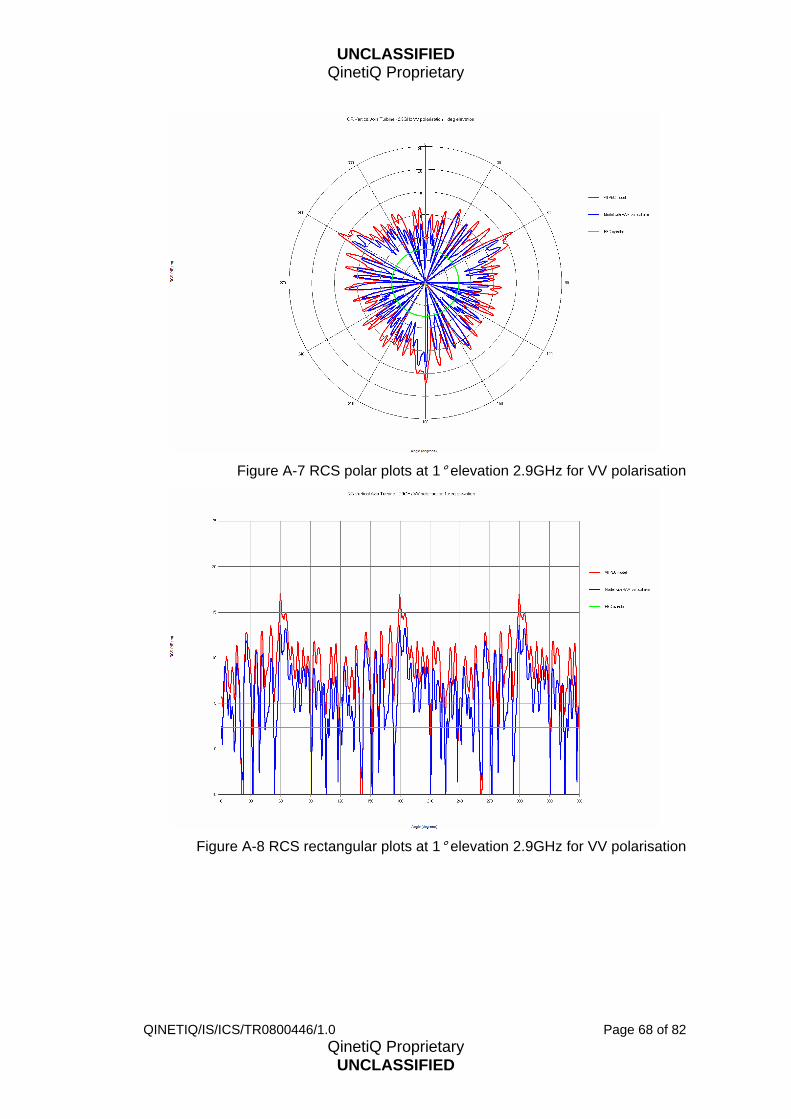
UNCLASSIFIED QinetiQ Proprietary
QINETIQ/IS/ICS/TR0800446/1.0 Page 68 of 82 QinetiQ Proprietary
UNCLASSIFIED
Figure A-7 RCS polar plots at 1° elevation 2.9GHz for VV polarisation
Figure A-8 RCS rectangular plots at 1° elevation 2.9GHz for VV polarisation

UNCLASSIFIED QinetiQ Proprietary
QINETIQ/IS/ICS/TR0800446/1.0 Page 69 of 82 QinetiQ Proprietary
UNCLASSIFIED
A.2 Hotspot and energy path displays for 1.3GHz
Figure A-9 Hotspot display of turbine assembly at 0° azimuth and 0° elevation 1.3GHz VV polarisation (peak A)
Figure A-10 Energy path display of turbine assembly at 0° azimuth and 0° elevation 1.3GHz VV polarisation (peak A)
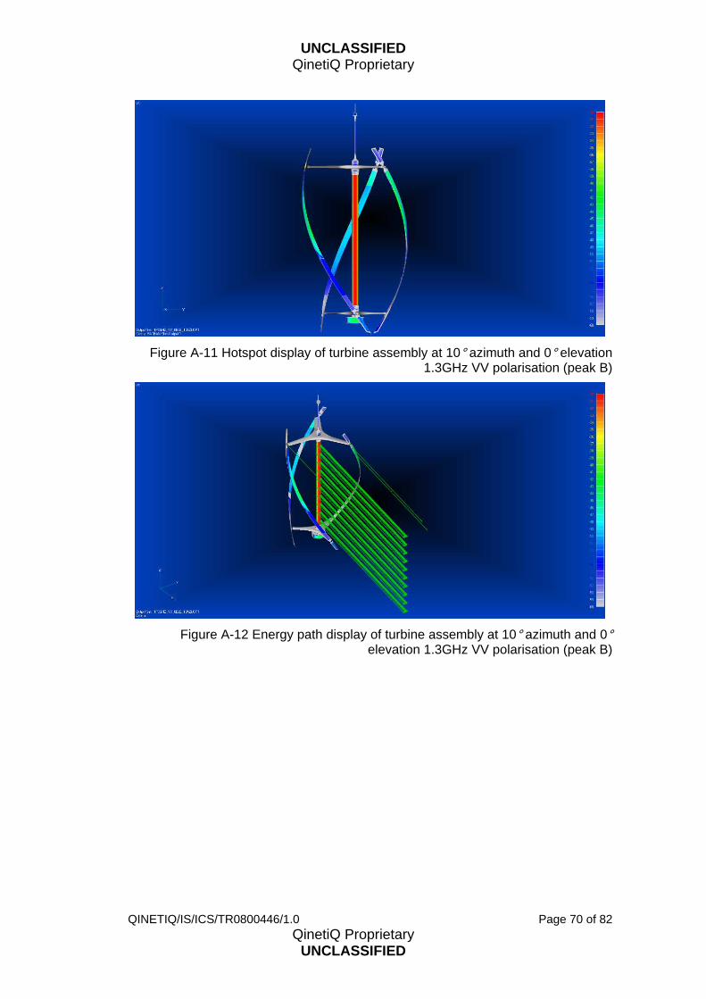
UNCLASSIFIED QinetiQ Proprietary
QINETIQ/IS/ICS/TR0800446/1.0 Page 70 of 82 QinetiQ Proprietary
UNCLASSIFIED
Figure A-11 Hotspot display of turbine assembly at 10° azimuth and 0° elevation 1.3GHz VV polarisation (peak B)
Figure A-12 Energy path display of turbine assembly at 10° azimuth and 0° elevation 1.3GHz VV polarisation (peak B)
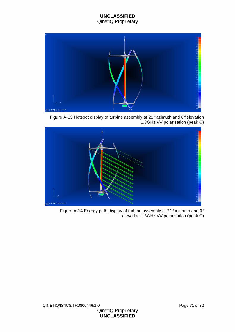
UNCLASSIFIED QinetiQ Proprietary
QINETIQ/IS/ICS/TR0800446/1.0 Page 71 of 82 QinetiQ Proprietary
UNCLASSIFIED
Figure A-13 Hotspot display of turbine assembly at 21° azimuth and 0° elevation 1.3GHz VV polarisation (peak C)
Figure A-14 Energy path display of turbine assembly at 21° azimuth and 0° elevation 1.3GHz VV polarisation (peak C)
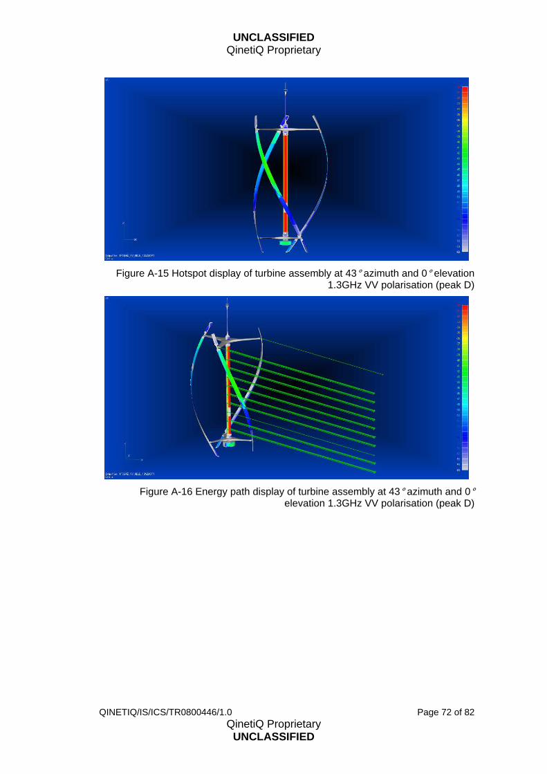
UNCLASSIFIED QinetiQ Proprietary
QINETIQ/IS/ICS/TR0800446/1.0 Page 72 of 82 QinetiQ Proprietary
UNCLASSIFIED
Figure A-15 Hotspot display of turbine assembly at 43° azimuth and 0° elevation 1.3GHz VV polarisation (peak D)
Figure A-16 Energy path display of turbine assembly at 43° azimuth and 0° elevation 1.3GHz VV polarisation (peak D)
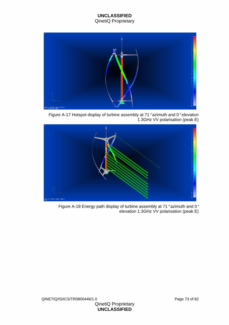
UNCLASSIFIED QinetiQ Proprietary
QINETIQ/IS/ICS/TR0800446/1.0 Page 73 of 82 QinetiQ Proprietary
UNCLASSIFIED
Figure A-17 Hotspot display of turbine assembly at 71° azimuth and 0° elevation 1.3GHz VV polarisation (peak E)
Figure A-18 Energy path display of turbine assembly at 71° azimuth and 0° elevation 1.3GHz VV polarisation (peak E)
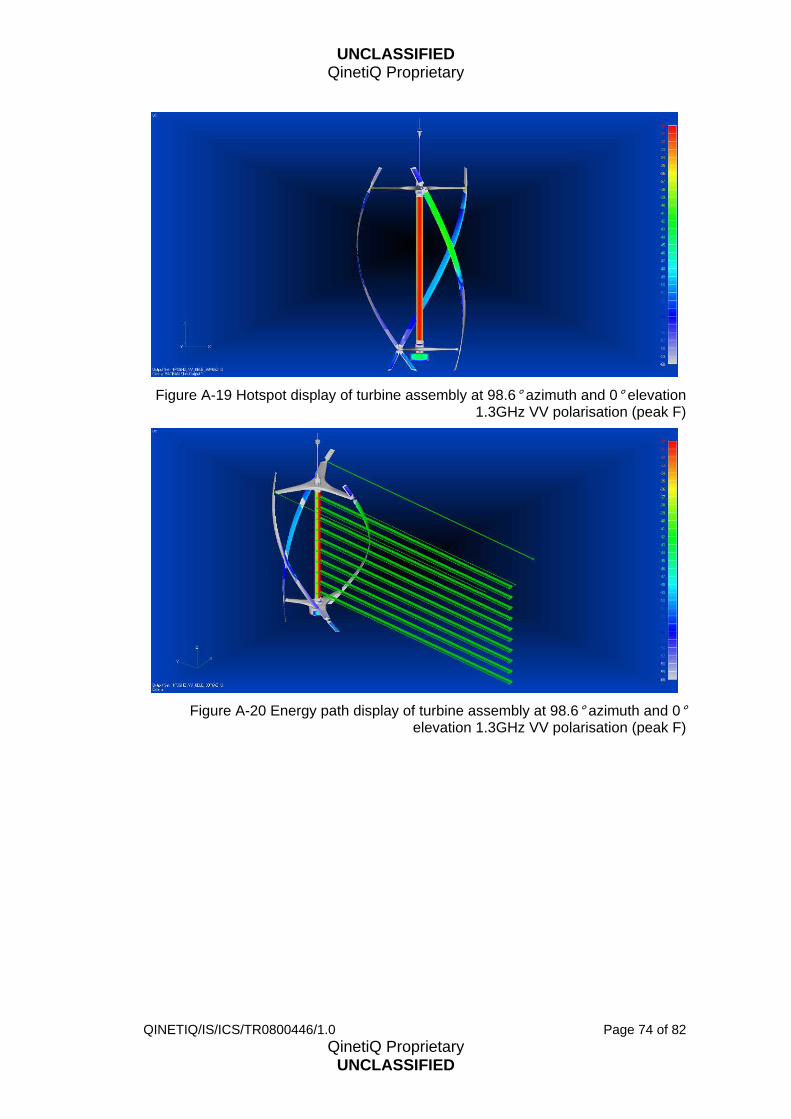
UNCLASSIFIED QinetiQ Proprietary
QINETIQ/IS/ICS/TR0800446/1.0 Page 74 of 82 QinetiQ Proprietary
UNCLASSIFIED
Figure A-19 Hotspot display of turbine assembly at 98.6° azimuth and 0° elevation 1.3GHz VV polarisation (peak F)
Figure A-20 Energy path display of turbine assembly at 98.6° azimuth and 0° elevation 1.3GHz VV polarisation (peak F)
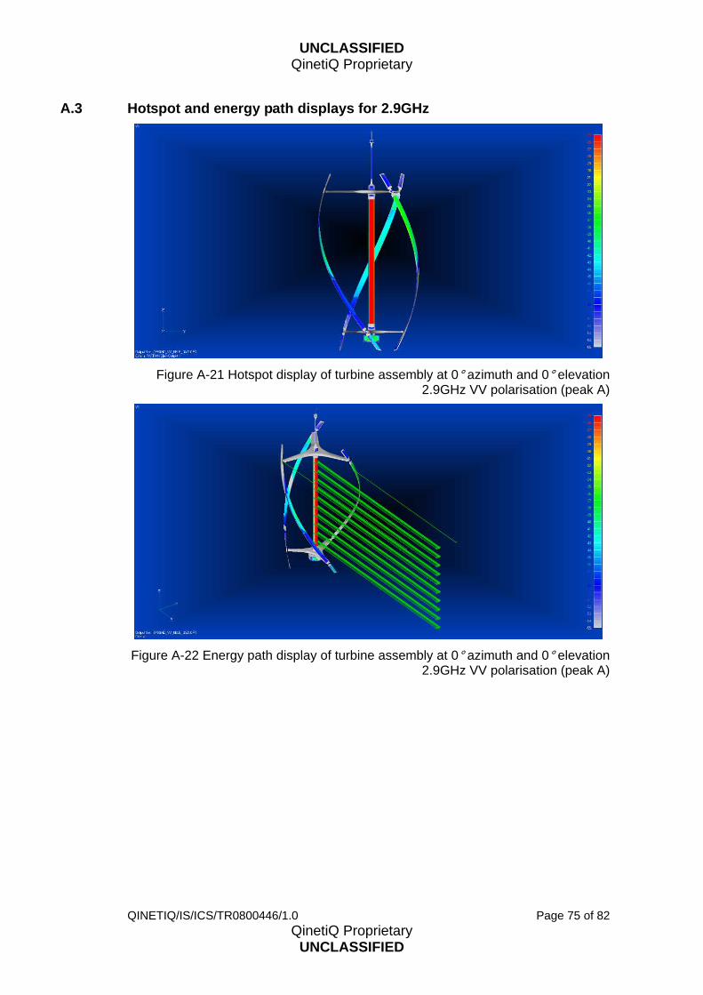
UNCLASSIFIED QinetiQ Proprietary
QINETIQ/IS/ICS/TR0800446/1.0 Page 75 of 82 QinetiQ Proprietary
UNCLASSIFIED
A.3 Hotspot and energy path displays for 2.9GHz
Figure A-21 Hotspot display of turbine assembly at 0° azimuth and 0° elevation 2.9GHz VV polarisation (peak A)
Figure A-22 Energy path display of turbine assembly at 0° azimuth and 0° elevation 2.9GHz VV polarisation (peak A)

UNCLASSIFIED QinetiQ Proprietary
QINETIQ/IS/ICS/TR0800446/1.0 Page 76 of 82 QinetiQ Proprietary
UNCLASSIFIED
Figure A-23 Hotspot display of turbine assembly at 25.1° azimuth and 0° elevation 2.9GHz VV polarisation (peak B)
Figure A-24 Energy path display of turbine assembly at 25.1° azimuth and 0° elevation 2.9GHz VV polarisation (peak B)

UNCLASSIFIED QinetiQ Proprietary
QINETIQ/IS/ICS/TR0800446/1.0 Page 77 of 82 QinetiQ Proprietary
UNCLASSIFIED
Figure A-25 Hotspot display of turbine assembly at 33.1° azimuth and 0° elevation 2.9GHz VV polarisation (peak C)
Figure A-26 Energy path display of turbine assembly at 33.1° azimuth and 0° elevation 2.9GHz VV polarisation (peak C)

UNCLASSIFIED QinetiQ Proprietary
QINETIQ/IS/ICS/TR0800446/1.0 Page 78 of 82 QinetiQ Proprietary
UNCLASSIFIED
Figure A-27 Hotspot display of turbine assembly at 56.3° azimuth and 0° elevation 2.9GHz VV polarisation (peak D)
Figure A-28 Energy path display of turbine assembly at 56.3° azimuth and 0° elevation 2.9GHz VV polarisation (peak D)
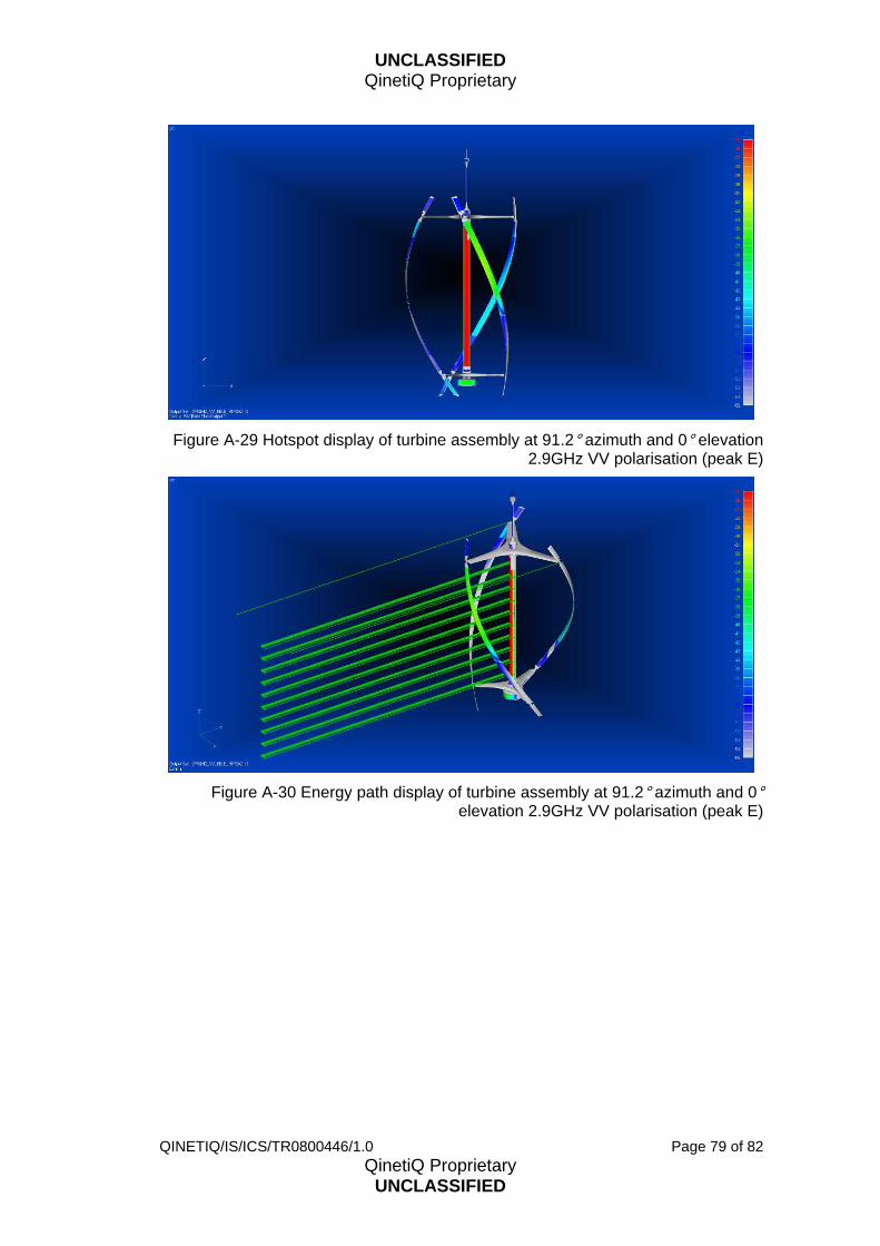
UNCLASSIFIED QinetiQ Proprietary
QINETIQ/IS/ICS/TR0800446/1.0 Page 79 of 82 QinetiQ Proprietary
UNCLASSIFIED
Figure A-29 Hotspot display of turbine assembly at 91.2° azimuth and 0° elevation 2.9GHz VV polarisation (peak E)
Figure A-30 Energy path display of turbine assembly at 91.2° azimuth and 0° elevation 2.9GHz VV polarisation (peak E)
UNCLASSIFIED QinetiQ Proprietary
QINETIQ/IS/ICS/TR0800446/1.0 Page 80 of 82 QinetiQ Proprietary
UNCLASSIFIED
Figure A-31 Hotspot display of turbine assembly at 109.4° azimuth and 0° elevation 2.9GHz VV polarisation (peak F)
Figure A-32 Energy path display of turbine assembly at 109.4° azimuth and 0° elevation 2.9GHz VV polarisation (peak F)

UNCLASSIFIED QinetiQ Proprietary
QINETIQ/IS/ICS/TR0800446/1.0 Page 81 of 82 QinetiQ Proprietary
UNCLASSIFIED
Initial distribution list External
Group Captain Maurice Dixon
QinetiQ
Information warehouse, QinetiQ Boscombe Down, Building 901, Salisbury, Wiltshire, SP4 0JP
File
UNCLASSIFIED QinetiQ Proprietary
QINETIQ/IS/ICS/TR0800446/1.0 Page 82 of 82 QinetiQ Proprietary
UNCLASSIFIED
Report documentation page Originator’s Report Number QINETIQ/IS/ICS/TR0800446
Originator’s Name and Location Chris New and Sebastian Di Laura, QinetiQ Portsdown Technology Park
Customer Contract Number and Period Covered
FTS2/025
Customer Sponsor’s Post/Name and Location
Group Captain Maurice Dixon
Report Protective Marking and any other markings
Date of issue Pagination No. of references
UK Secret QinetiQ Proprietary July 2008 Cover + 82 8
Report Title
Vertical Axis Wind Turbine – Radar Cross Section Assessment
Translation / Conference details N/A
Title Protective Marking Unclassified
Authors Chris New, Sebastian Di Laura
Downgrading Statement Review after 5 years
Secondary Release Limitations
Announcement Limitations
Keywords / Descriptors Radar cross section, vertical axis wind turbine
Abstract
QinetiQ was contracted by the Air Defence and Air Traffic Services Integrated Project Team to predict and measure the radar cross section (RCS) of a Quiet Revolution vertical axis wind turbine (VAWT), as well as assess the potential impact it would have on radar.
The RCS predictions have been calculated at 1.3GHz and 2.9GHz for a perfect electric conductor material turbine assembly and in free space, using the QinetiQ RCS prediction tool, Spectre®. These results were then compared to real radar measurement trials of a Quiet Revolution qr5, undertaken at the QinetiQ Funtington measurement.
The final data comparisons showed good agreement between measured and modelled data, although some difference were highlight, and were likely to be caused by difference in the computer aided design model. It was concluded that a VAWT will add any additional clutter levels to that of what is already seen and dealt with by a radar.
Abstract Protective Marking: UNCLASSIFIED
This form meets DRIC-SPEC 1000 issue 7