Vertical Antenna Ground Systems At HF

Rudy Severns N6LF

Introduction A key factor in determining the radiation efficiency of verticals is the power loss in the soil around 1 the antenna. Minimizing this loss is the purpose of the ground system associated with a vertical. A great deal of analytical and experimental work has been done over the past 100 years on the design and performance of ground systems for verticals. The most influential for amateurs was the work by George Brown in the 1930's which set the standard for broadcast (BC) antennas to this day. For the most part, discussions in amateur literature are direct extensions of BC experience [1-3]. Hams have tended to view the BC work as gospel. Maybe it's time to take a look at just how well BC work applies to HF applications. Brown [4,5] and other workers [6-9] were primarily concerned with frequencies where most soils are basically resistive - i.e. BC band and down. Making the assumption that the ground is resistive greatly simplifies the analysis and is usually valid at those frequencies at least for any soil you would like to have for a BC station. Hams on the other hand are more interested in HF where soil characteristics become a combination of reactive and resistive. This changes the loss characteristics and, to some extent, the design of the ground system2. To make this discussion more readable I have eliminated most of the math 3. The few math expressions which do appear can be passed over without losing the gist. Important ideas are illustrated using graphs 4. Overview of Ground Loss In Brown's work, ground losses were calculated by assuming the soil was basically resistive. The current in the soil was determined from the magnetic field intensity along the ground surface (H) and the relative distribution of current between the soil (Ie) and the ground system (Ir). The effective resistance (R) was determined from skin depth and soil conductivity. Ground loss was simply Ie2R. This scheme took into account the change in loss due to the reduced skin depth as frequency is increased but it did not include the complex impedance of soil which becomes important at HF. The expression for skin depth used was also an approximation for a good conductor not a lossy dielectric which soil is at HF. Frank Abbott [19] introduced a much more general method for calculating ground loss that is valid at HF 5. His method is what I use. We can compare the two calculation methods by simply taking the ratio of the power loss a 'la Abbott divided by that from Brown as shown in figure 1.

1 roughly within a wavelength 2 Brown, Lewis and Epstein did their field measurements at 3 MHz but the basic calculations were for resistive ground which is valid at 3 MHz only for very good ground. 3 For those who want the math I can supply it on request. 4 I can provide additional graphs on request.

1

5 It is interesting that 99% of Abbott's paper uses a resistive ground approximation. This is not surprising since he was concerned with BC antennas. Only in one short paragraph on page 847 does he give the general expression for power loss in complex ground, which I have used.

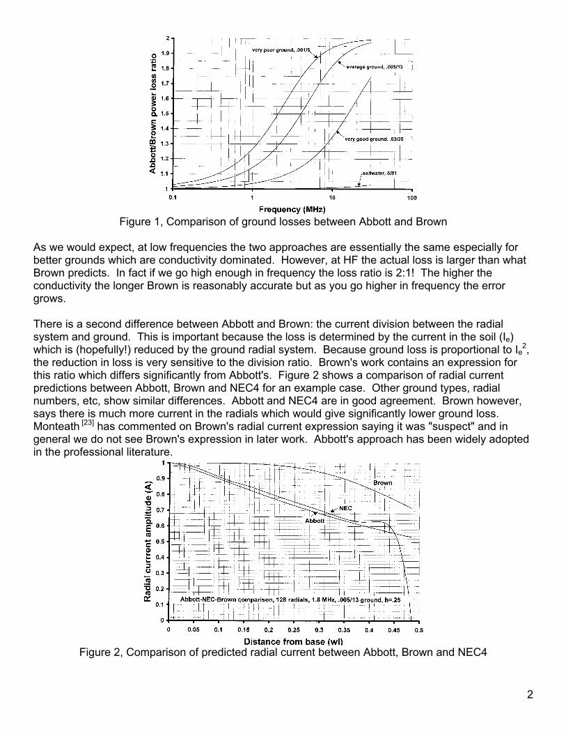
Figure 1, Comparison of ground losses between Abbott and Brown

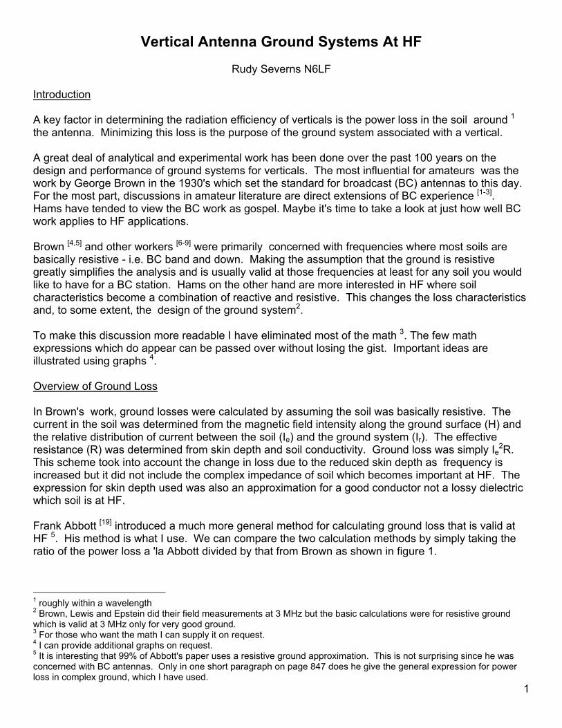
As we would expect, at low frequencies the two approaches are essentially the same especially for better grounds which are conductivity dominated. However, at HF the actual loss is larger than what Brown predicts. In fact if we go high enough in frequency the loss ratio is 2:1! The higher the conductivity the longer Brown is reasonably accurate but as you go higher in frequency the error grows. There is a second difference between Abbott and Brown: the current division between the radial system and ground. This is important because the loss is determined by the current in the soil (Ie) which is (hopefully!) reduced by the ground radial system. Because ground loss is proportional to Ie2, the reduction in loss is very sensitive to the division ratio. Brown's work contains an expression for this ratio which differs significantly from Abbott's. Figure 2 shows a comparison of radial current predictions between Abbott, Brown and NEC4 for an example case. Other ground types, radial numbers, etc, show similar differences. Abbott and NEC4 are in good agreement. Brown however, says there is much more current in the radials which would give significantly lower ground loss. Monteath [23] has commented on Brown's radial current expression saying it was "suspect" and in general we do not see Brown's expression in later work. Abbott's approach has been widely adopted in the professional literature.

Figure 2, Comparison of predicted radial current between Abbott, Brown and NEC4

2

Before getting into the details of determining Rg we need to take a look at the H-fields near the antenna which are inducing the ground currents and the concept of ground impedance. I will be ignoring the E-field losses which are usually small for antenna heights of 0.125 - 0.25 wl (wavelength) which is a normal range for ham antennas. Be warned however, for shorter antennas the E-field losses are significant and cannot be ignored. E and H-fields around a vertical To assist in making comparisons between antennas of different heights (h) 6, the majority of my graphs will assume constant radiated power (Pr). This is equivalent to 36.6 W into an idealized 0.25 wl vertical with the radiation resistance (Rr) equal to 36.6 Ohms and base current (Io) of 1 Arms. For different values of h we will change Io to compensate for the change in Rr to keep Pr constant at 36.6 W. This is an approximation but it gives a feeling for the effect of h on ground losses 7. In the end when we calculate the effective ground resistance (Rg), the values for Io cancel out but they are handy in the discussion before we get to that point. Ground currents are directly proportional to the magnetic field intensity (H) at the ground surface. For a given h we can calculate H and figure 3 is an example of H for verticals with h in the range of 0.05 to 0.25 wl and f = 1.8 MHz, over perfect ground.

Figure 3, H at the ground surface for various antenna heights and constant Pr = 37 W.

Notice that as we shorten the antenna 8, H increases near the base. This means greater ground loss as we shorten the antenna at a given frequency for a given ground system. There will also be a change in H

6 usually in wavelengths

7 A more detailed discussion of the effect of antenna height and height-to-diameter ratio on Rr and the corresponding values of Io can be found in reference 22.

38 for the same Pr

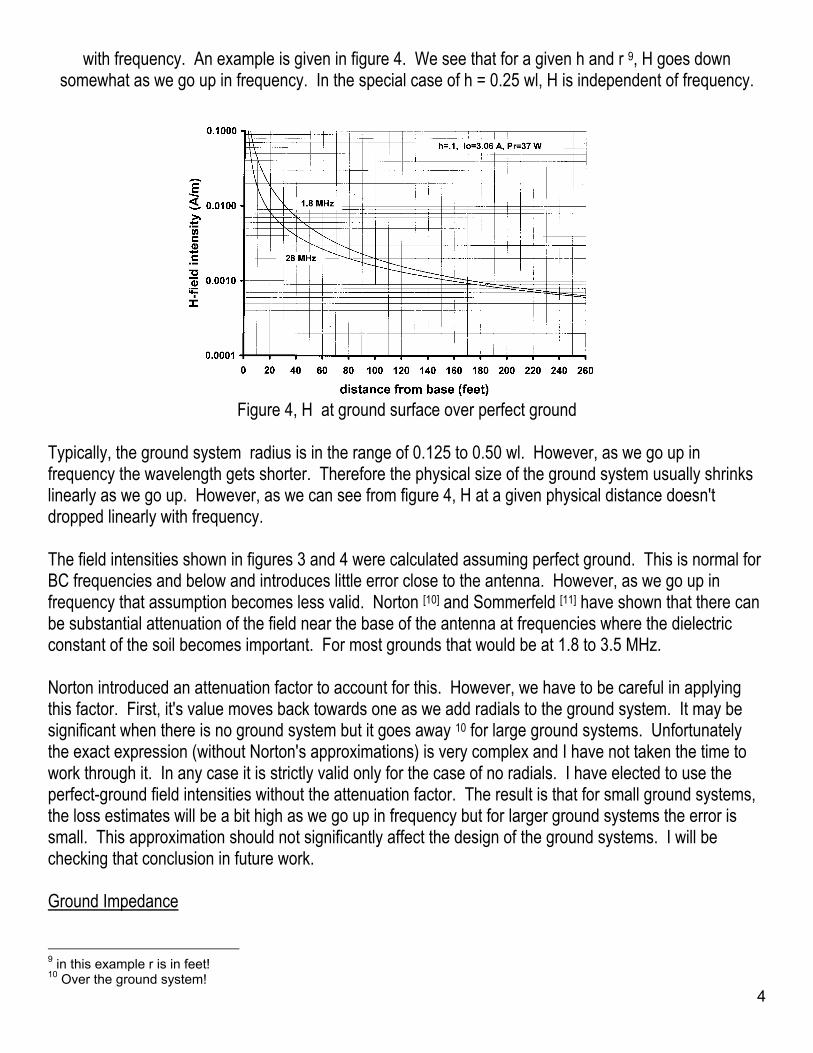
with frequency. An example is given in figure 4. We see that for a given h and r 9, H goes down somewhat as we go up in frequency. In the special case of h = 0.25 wl, H is independent of frequency.

Figure 4, H at ground surface over perfect ground Typically, the ground system radius is in the range of 0.125 to 0.50 wl. However, as we go up in frequency the wavelength gets shorter. Therefore the physical size of the ground system usually shrinks linearly as we go up. However, as we can see from figure 4, H at a given physical distance doesn't dropped linearly with frequency. The field intensities shown in figures 3 and 4 were calculated assuming perfect ground. This is normal for BC frequencies and below and introduces little error close to the antenna. However, as we go up in frequency that assumption becomes less valid. Norton [10] and Sommerfeld [11] have shown that there can be substantial attenuation of the field near the base of the antenna at frequencies where the dielectric constant of the soil becomes important. For most grounds that would be at 1.8 to 3.5 MHz. Norton introduced an attenuation factor to account for this. However, we have to be careful in applying this factor. First, it's value moves back towards one as we add radials to the ground system. It may be significant when there is no ground system but it goes away 10 for large ground systems. Unfortunately the exact expression (without Norton's approximations) is very complex and I have not taken the time to work through it. In any case it is strictly valid only for the case of no radials. I have elected to use the perfect-ground field intensities without the attenuation factor. The result is that for small ground systems, the loss estimates will be a bit high as we go up in frequency but for larger ground systems the error is small. This approximation should not significantly affect the design of the ground systems. I will be checking that conclusion in future work. Ground Impedance 9 in this example r is in feet!

410 Over the ground system!

Ground impedance (Zg) is analogous to the surge impedance (Zo) of a transmission line. The connection being that a wave traveling along a transmission line is similar to a wave propagating in soil. We can do a similar thing with soil and derive what we call the intrinsic impedance:

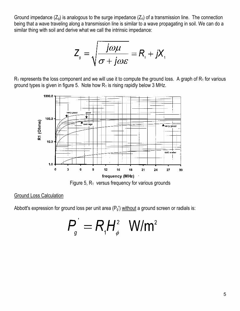
R1 represents the loss component and we will use it to compute the ground loss. A graph of R1 for various ground types is given in figure 5. Note how R1 is rising rapidly below 3 MHz.

Figure 5, R1 versus frequency for various grounds Ground Loss Calculation Abbott's expression for ground loss per unit area (Pg') without a ground screen or radials is:

5

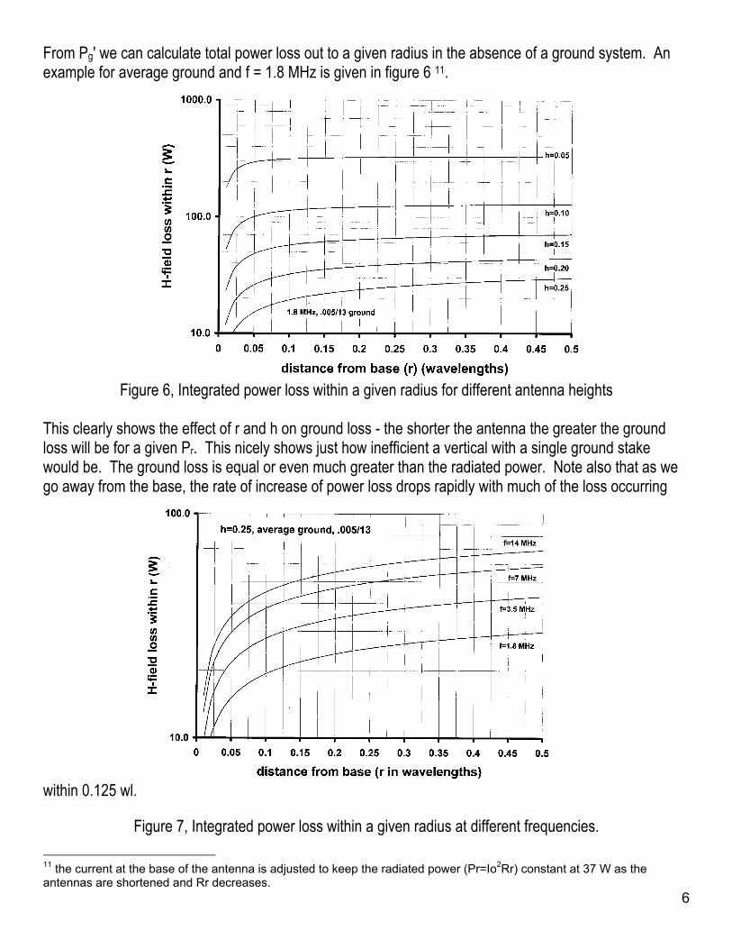
From Pg' we can calculate total power loss out to a given radius in the absence of a ground system. An example for average ground and f = 1.8 MHz is given in figure 6 11.

Figure 6, Integrated power loss within a given radius for different antenna heights

This clearly shows the effect of r and h on ground loss - the shorter the antenna the greater the ground loss will be for a given Pr. This nicely shows just how inefficient a vertical with a single ground stake would be. The ground loss is equal or even much greater than the radiated power. Note also that as we go away from the base, the rate of increase of power loss drops rapidly with much of the loss occurring

within 0.125 wl.

Figure 7, Integrated power loss within a given radius at different frequencies.

6

11 the current at the base of the antenna is adjusted to keep the radiated power (Pr=Io2Rr) constant at 37 W as the antennas are shortened and Rr decreases.

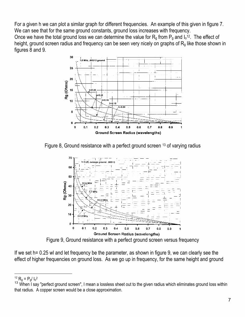
For a given h we can plot a similar graph for different frequencies. An example of this given in figure 7. We can see that for the same ground constants, ground loss increases with frequency. Once we have the total ground loss we can determine the value for Rg from Pg and Io12. The effect of height, ground screen radius and frequency can be seen very nicely on graphs of Rg like those shown in figures 8 and 9.

Figure 8, Ground resistance with a perfect ground screen 13 of varying radius

Figure 9, Ground resistance with a perfect ground screen versus frequency

If we set h= 0.25 wl and let frequency be the parameter, as shown in figure 9, we can clearly see the effect of higher frequencies on ground loss. As we go up in frequency, for the same height and ground

12 Rg = Pg/ Io2 13 When I say "perfect ground screen", I mean a lossless sheet out to the given radius which eliminates ground loss within that radius. A copper screen would be a close approximation.

7

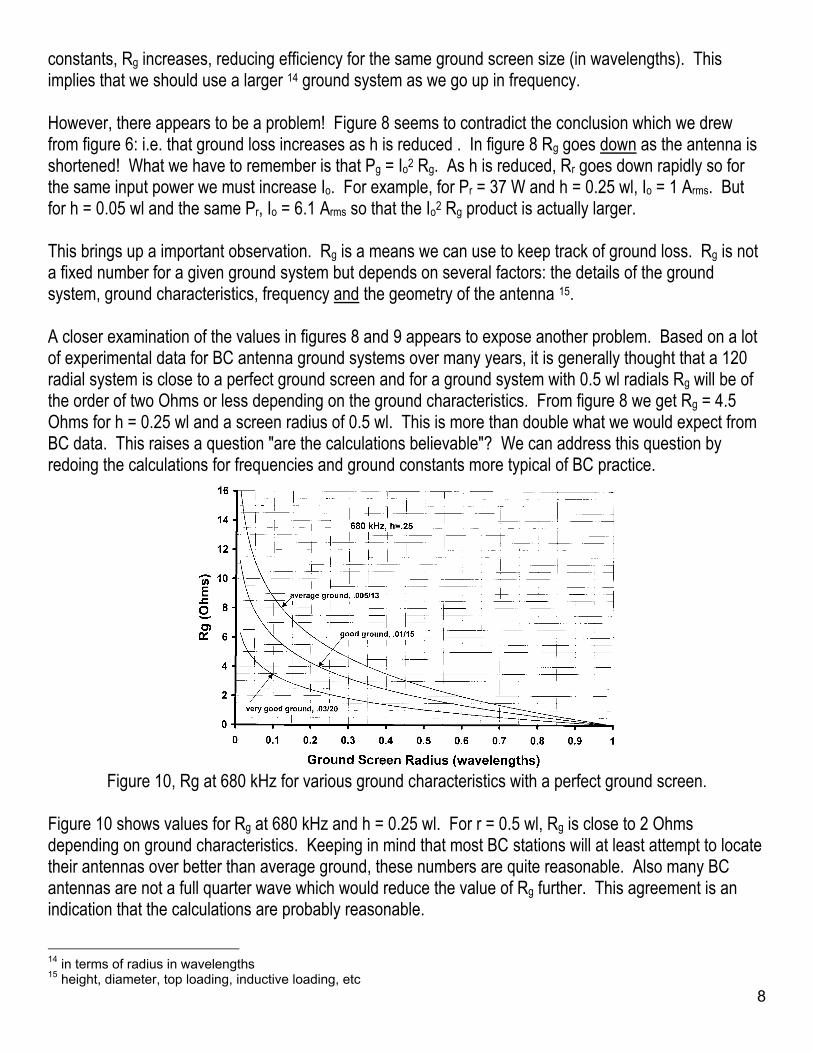
constants, Rg increases, reducing efficiency for the same ground screen size (in wavelengths). This implies that we should use a larger 14 ground system as we go up in frequency. However, there appears to be a problem! Figure 8 seems to contradict the conclusion which we drew from figure 6: i.e. that ground loss increases as h is reduced . In figure 8 Rg goes down as the antenna is shortened! What we have to remember is that Pg = Io2 Rg. As h is reduced, Rr goes down rapidly so for the same input power we must increase Io. For example, for Pr = 37 W and h = 0.25 wl, Io = 1 Arms. But for h = 0.05 wl and the same Pr, Io = 6.1 Arms so that the Io2 Rg product is actually larger. This brings up a important observation. Rg is a means we can use to keep track of ground loss. Rg is not a fixed number for a given ground system but depends on several factors: the details of the ground system, ground characteristics, frequency and the geometry of the antenna 15. A closer examination of the values in figures 8 and 9 appears to expose another problem. Based on a lot of experimental data for BC antenna ground systems over many years, it is generally thought that a 120 radial system is close to a perfect ground screen and for a ground system with 0.5 wl radials Rg will be of the order of two Ohms or less depending on the ground characteristics. From figure 8 we get Rg = 4.5 Ohms for h = 0.25 wl and a screen radius of 0.5 wl. This is more than double what we would expect from BC data. This raises a question "are the calculations believable"? We can address this question by redoing the calculations for frequencies and ground constants more typical of BC practice.

Figure 10, Rg at 680 kHz for various ground characteristics with a perfect ground screen.

Figure 10 shows values for Rg at 680 kHz and h = 0.25 wl. For r = 0.5 wl, Rg is close to 2 Ohms depending on ground characteristics. Keeping in mind that most BC stations will at least attempt to locate their antennas over better than average ground, these numbers are quite reasonable. Also many BC antennas are not a full quarter wave which would reduce the value of Rg further. This agreement is an indication that the calculations are probably reasonable.

14 in terms of radius in wavelengths

815 height, diameter, top loading, inductive loading, etc

Ground Current Division Ratio For Radial Ground Systems To this point we've assumed either no ground system or a perfect ground screen. Obviously a perfect ground screen is usually not practical. The most common ground system for a vertical is a series of radial ground wires, on or below the ground surface, arranged symmetrically around the base. The purpose of the radial system is to divert current from the soil into the radial conductors which have very low loss compared to soil. We can calculate the current division between a radial system and the soil and use this to determine Rg. We do this by assuming that the radial system has an impedance Zr, again analogous to a transmission line. Zr is in parallel with Zg so Ie is divided between the two impedances depending on their relative values:

1

1

1

g r

ge r g

r

I ZFZI Z ZZ

≡ = =+

+

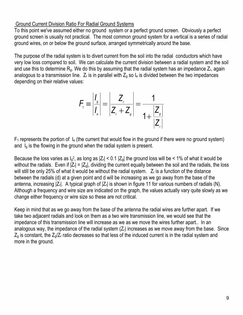
F1 represents the portion of Ie (the current that would flow in the ground if there were no ground system) and Ig is the flowing in the ground when the radial system is present. Because the loss varies as Ig2, as long as |Zr| < 0.1 |Zg| the ground loss will be < 1% of what it would be without the radials. Even if |Zr| = |Zg|, dividing the current equally between the soil and the radials, the loss will still be only 25% of what it would be without the radial system. Zr is a function of the distance between the radials (d) at a given point and d will be increasing as we go away from the base of the antenna, increasing |Zr|. A typical graph of |Zr| is shown in figure 11 for various numbers of radials (N). Although a frequency and wire size are indicated on the graph, the values actually vary quite slowly as we change either frequency or wire size so these are not critical. Keep in mind that as we go away from the base of the antenna the radial wires are further apart. If we take two adjacent radials and look on them as a two wire transmission line, we would see that the impedance of this transmission line will increase as we as we move the wires further apart.. In an analogous way, the impedance of the radial system (Zr) increases as we move away from the base. Since Zg is constant, the Zg/Zr ratio decreases so that less of the induced current is in the radial system and more in the ground.

9

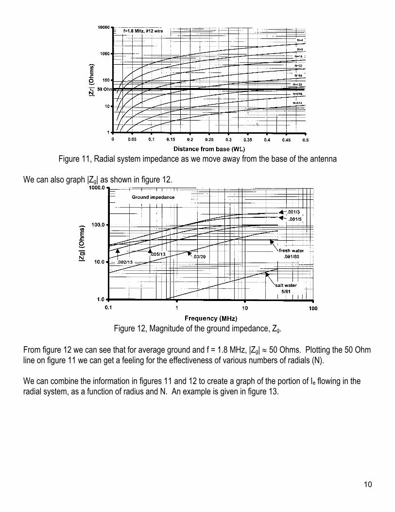
Figure 11, Radial system impedance as we move away from the base of the antenna

We can also graph |Zg| as shown in figure 12.

Figure 12, Magnitude of the ground impedance, Zg.

From figure 12 we can see that for average ground and f = 1.8 MHz, |Zg| ≈ 50 Ohms. Plotting the 50 Ohm line on figure 11 we can get a feeling for the effectiveness of various numbers of radials (N). We can combine the information in figures 11 and 12 to create a graph of the portion of Ie flowing in the radial system, as a function of radius and N. An example is given in figure 13.

10

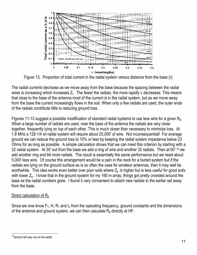
Figure 13, Proportion of total current in the radial system versus distance from the base (r).

The radial currents decrease as we move away from the base because the spacing between the radial wires is increasing which increases Zr. The fewer the radials, the more rapidly Ir decreases. This means that close to the base of the antenna most of the current is in the radial system, but as we move away from the base the current increasingly flows in the soil. When only a few radials are used, the outer ends of the radials contribute little to reducing ground loss. Figures 11-13 suggest a possible modification of standard radial systems to use less wire for a given Rg. When a large number of radials are used, near the base of the antenna the radials are very close together, frequently lying on top of each other. This is much closer than necessary to minimize loss. At 1.8 MHz a 128 1/4 wl radial system will require about 25,000' of wire. Not inconsequential! For average ground we can reduce the ground loss to 10% or less by keeping the radial system impedance below 23 Ohms for as long as possible. A simple calculation shows that we can meet this criterion by starting with a 32 radial system. At 30' out from the base we add a ring of wire and another 32 radials. Then at 60' 16 we add another ring and 64 more radials. The result is essentially the same performance but we need about 5,000' less wire. Of course this arrangement would be a pain in the neck for a buried system but if the radials are lying on the ground surface as is so often the case for amateur antennas, then it may well be worthwhile. This idea works even better over poor soils where Zg is higher but is less useful for good soils with lower Zg. I know that in the ground system for my 160 m array, things got pretty crowded around the base as the radial numbers grew. I found it very convenient to attach new radials to the earlier set away from the base. Direct calculation of Rg Since we now know F1, H, R1 and Io from the operating frequency, ground constants and the dimensions of the antenna and ground system, we can then calculate Rg directly at HF:

1116almost half way out on the radial

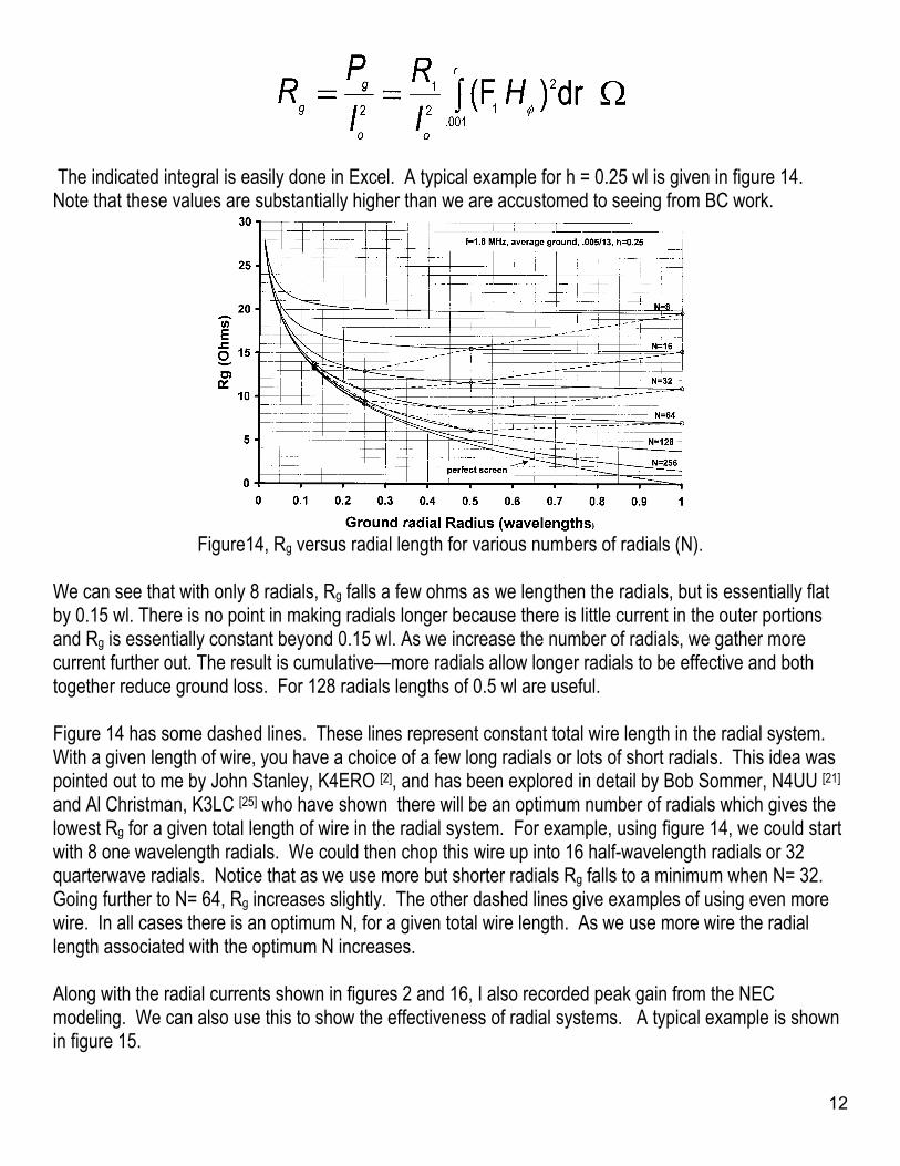
The indicated integral is easily done in Excel. A typical example for h = 0.25 wl is given in figure 14. Note that these values are substantially higher than we are accustomed to seeing from BC work.

Figure14, Rg versus radial length for various numbers of radials (N).

We can see that with only 8 radials, Rg falls a few ohms as we lengthen the radials, but is essentially flat by 0.15 wl. There is no point in making radials longer because there is little current in the outer portions and Rg is essentially constant beyond 0.15 wl. As we increase the number of radials, we gather more current further out. The result is cumulative—more radials allow longer radials to be effective and both together reduce ground loss. For 128 radials lengths of 0.5 wl are useful. Figure 14 has some dashed lines. These lines represent constant total wire length in the radial system. With a given length of wire, you have a choice of a few long radials or lots of short radials. This idea was pointed out to me by John Stanley, K4ERO [2], and has been explored in detail by Bob Sommer, N4UU [21] and Al Christman, K3LC [25] who have shown there will be an optimum number of radials which gives the lowest Rg for a given total length of wire in the radial system. For example, using figure 14, we could start with 8 one wavelength radials. We could then chop this wire up into 16 half-wavelength radials or 32 quarterwave radials. Notice that as we use more but shorter radials Rg falls to a minimum when N= 32. Going further to N= 64, Rg increases slightly. The other dashed lines give examples of using even more wire. In all cases there is an optimum N, for a given total wire length. As we use more wire the radial length associated with the optimum N increases. Along with the radial currents shown in figures 2 and 16, I also recorded peak gain from the NEC modeling. We can also use this to show the effectiveness of radial systems. A typical example is shown in figure 15.

12

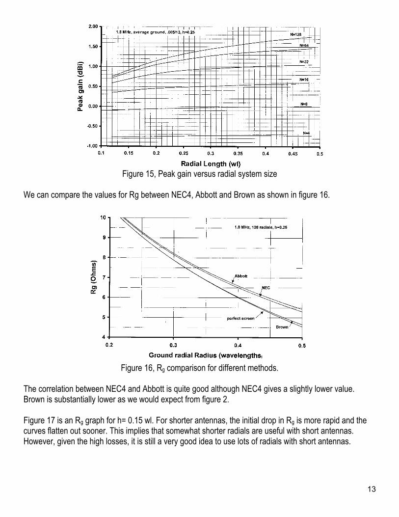
Figure 15, Peak gain versus radial system size

We can compare the values for Rg between NEC4, Abbott and Brown as shown in figure 16.

Figure 16, Rg comparison for different methods.

The correlation between NEC4 and Abbott is quite good although NEC4 gives a slightly lower value. Brown is substantially lower as we would expect from figure 2. Figure 17 is an Rg graph for h= 0.15 wl. For shorter antennas, the initial drop in Rg is more rapid and the curves flatten out sooner. This implies that somewhat shorter radials are useful with short antennas. However, given the high losses, it is still a very good idea to use lots of radials with short antennas.

13

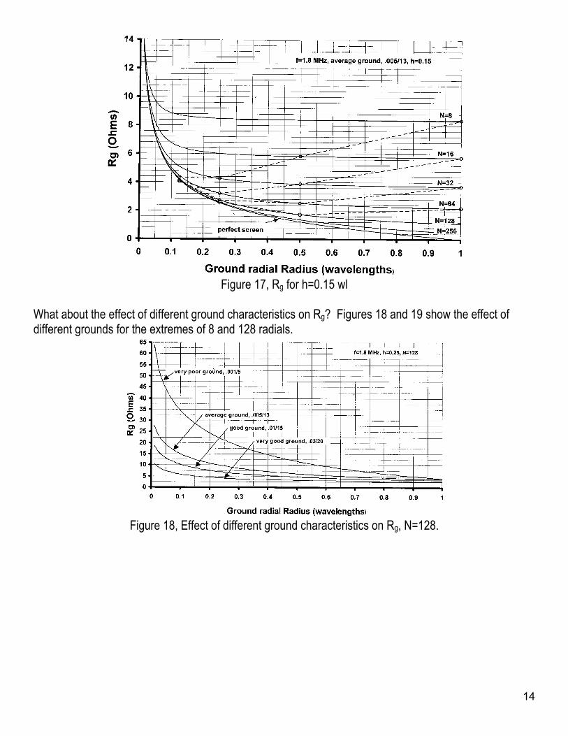
Figure 17, Rg for h=0.15 wl

What about the effect of different ground characteristics on Rg? Figures 18 and 19 show the effect of different grounds for the extremes of 8 and 128 radials.

Figure 18, Effect of different ground characteristics on Rg, N=128.

14

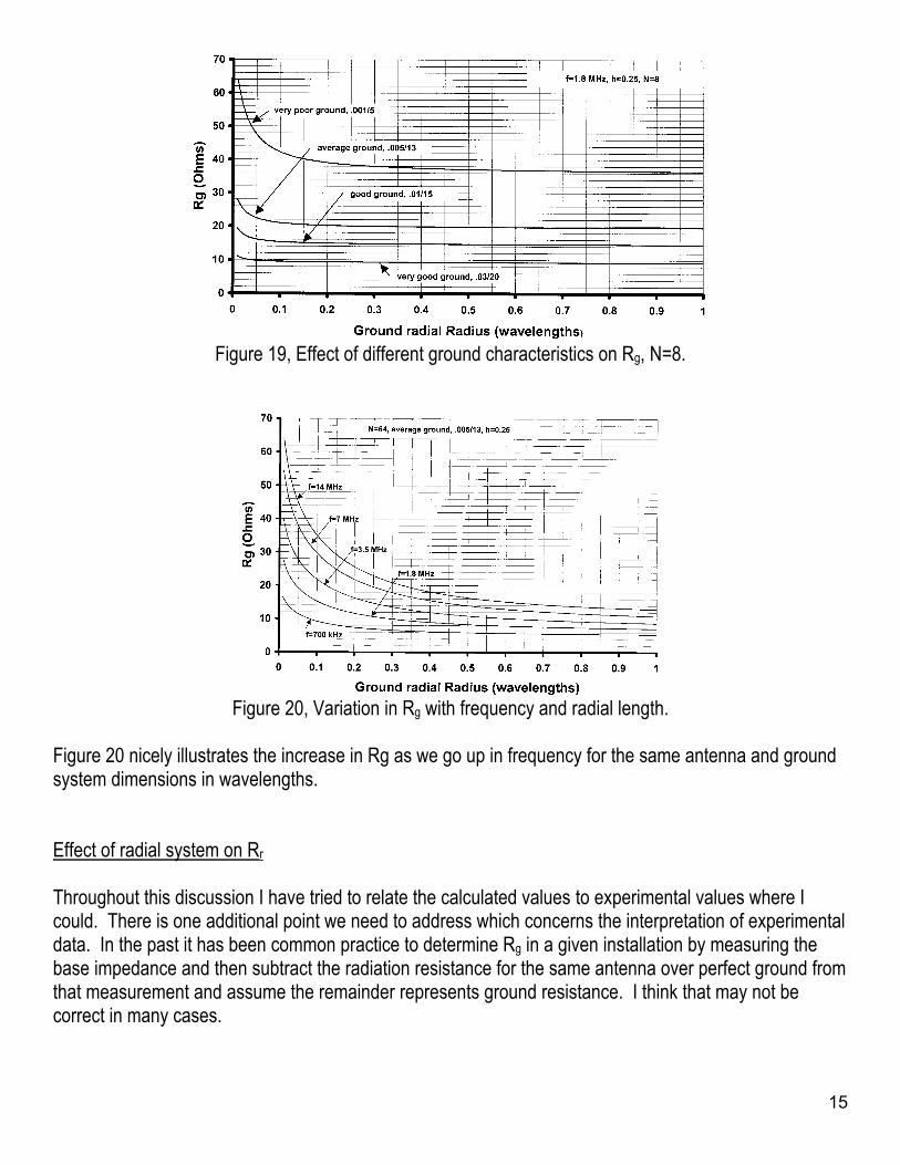
Figure 19, Effect of different ground characteristics on Rg, N=8.

Figure 20, Variation in Rg with frequency and radial length.

Figure 20 nicely illustrates the increase in Rg as we go up in frequency for the same antenna and ground system dimensions in wavelengths.

Effect of radial system on Rr Throughout this discussion I have tried to relate the calculated values to experimental values where I could. There is one additional point we need to address which concerns the interpretation of experimental data. In the past it has been common practice to determine Rg in a given installation by measuring the base impedance and then subtract the radiation resistance for the same antenna over perfect ground from that measurement and assume the remainder represents ground resistance. I think that may not be correct in many cases.

15

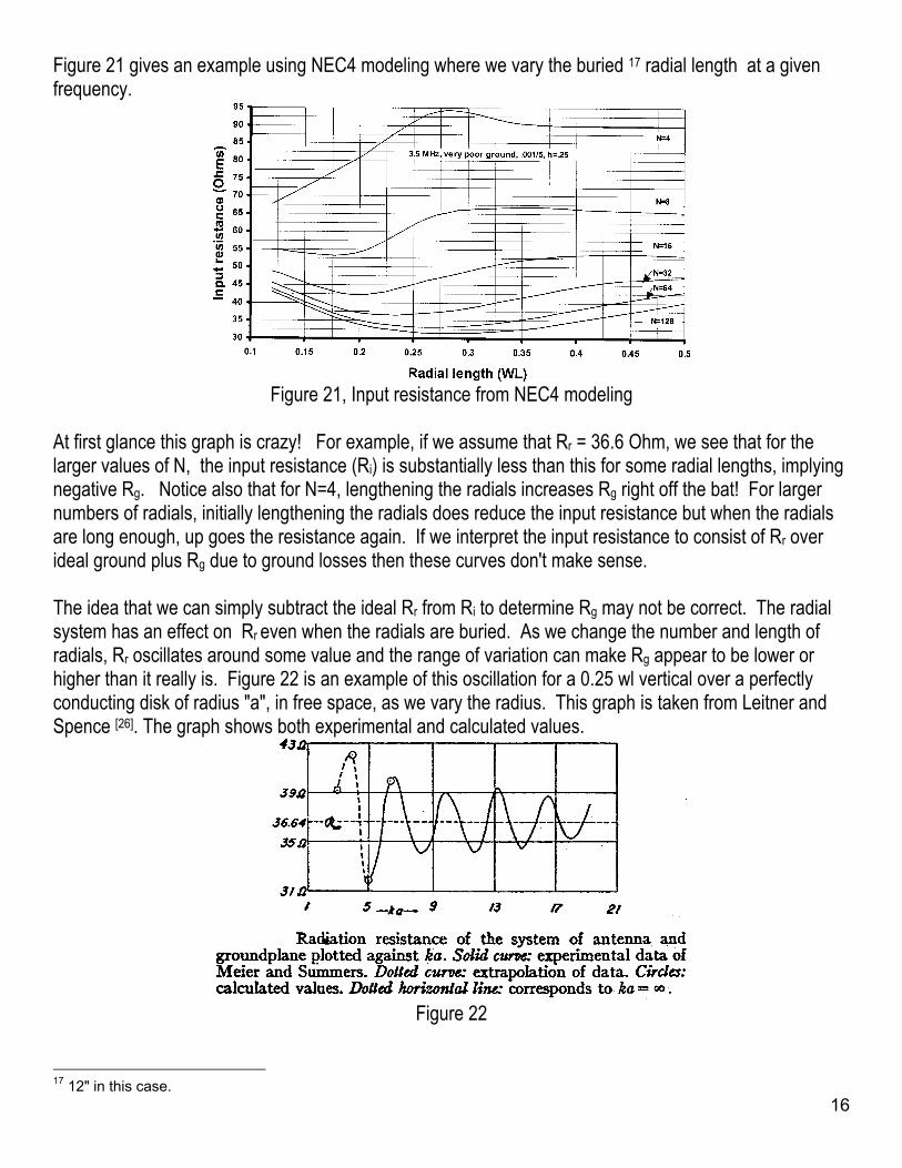
Figure 21 gives an example using NEC4 modeling where we vary the buried 17 radial length at a given frequency.

Figure 21, Input resistance from NEC4 modeling

At first glance this graph is crazy! For example, if we assume that Rr = 36.6 Ohm, we see that for the larger values of N, the input resistance (Ri) is substantially less than this for some radial lengths, implying negative Rg. Notice also that for N=4, lengthening the radials increases Rg right off the bat! For larger numbers of radials, initially lengthening the radials does reduce the input resistance but when the radials are long enough, up goes the resistance again. If we interpret the input resistance to consist of Rr over ideal ground plus Rg due to ground losses then these curves don't make sense. The idea that we can simply subtract the ideal Rr from Ri to determine Rg may not be correct. The radial system has an effect on Rr even when the radials are buried. As we change the number and length of radials, Rr oscillates around some value and the range of variation can make Rg appear to be lower or higher than it really is. Figure 22 is an example of this oscillation for a 0.25 wl vertical over a perfectly conducting disk of radius "a", in free space, as we vary the radius. This graph is taken from Leitner and Spence [26]. The graph shows both experimental and calculated values.

Figure 22

1617 12" in this case.

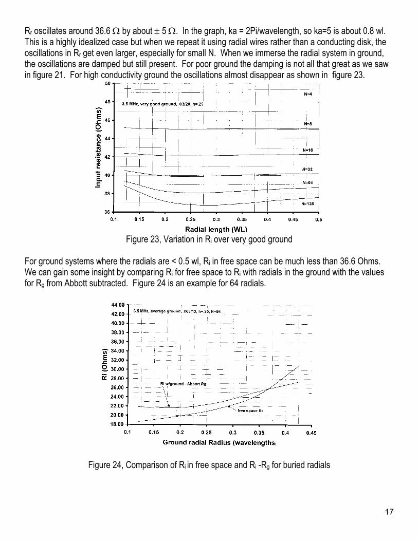
Rr oscillates around 36.6 Ω by about ± 5 Ω. In the graph, ka = 2Pi/wavelength, so ka=5 is about 0.8 wl. This is a highly idealized case but when we repeat it using radial wires rather than a conducting disk, the oscillations in Rr get even larger, especially for small N. When we immerse the radial system in ground, the oscillations are damped but still present. For poor ground the damping is not all that great as we saw in figure 21. For high conductivity ground the oscillations almost disappear as shown in figure 23.

Figure 23, Variation in Ri over very good ground

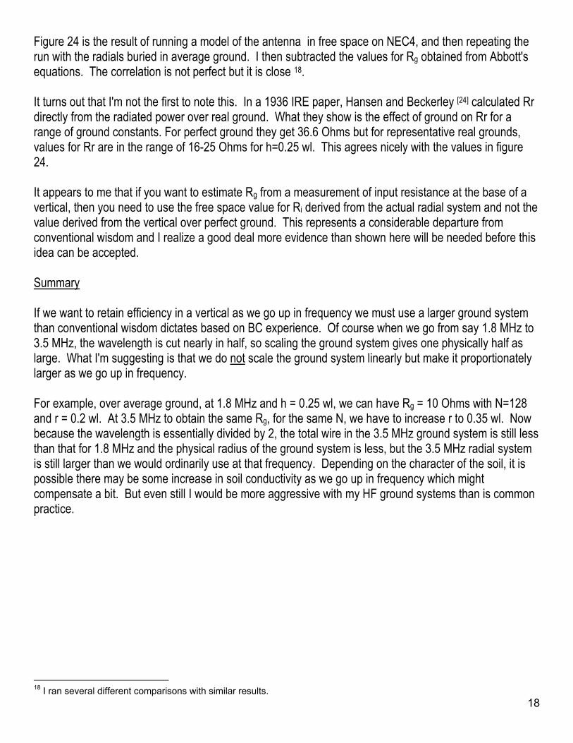
For ground systems where the radials are < 0.5 wl, Ri in free space can be much less than 36.6 Ohms. We can gain some insight by comparing Ri for free space to Ri with radials in the ground with the values for Rg from Abbott subtracted. Figure 24 is an example for 64 radials.

Figure 24, Comparison of Ri in free space and Ri -Rg for buried radials

17

18

Figure 24 is the result of running a model of the antenna in free space on NEC4, and then repeating the run with the radials buried in average ground. I then subtracted the values for Rg obtained from Abbott's equations. The correlation is not perfect but it is close 18. It turns out that I'm not the first to note this. In a 1936 IRE paper, Hansen and Beckerley [24] calculated Rr directly from the radiated power over real ground. What they show is the effect of ground on Rr for a range of ground constants. For perfect ground they get 36.6 Ohms but for representative real grounds, values for Rr are in the range of 16-25 Ohms for h=0.25 wl. This agrees nicely with the values in figure 24. It appears to me that if you want to estimate Rg from a measurement of input resistance at the base of a vertical, then you need to use the free space value for Ri derived from the actual radial system and not the value derived from the vertical over perfect ground. This represents a considerable departure from conventional wisdom and I realize a good deal more evidence than shown here will be needed before this idea can be accepted. Summary If we want to retain efficiency in a vertical as we go up in frequency we must use a larger ground system than conventional wisdom dictates based on BC experience. Of course when we go from say 1.8 MHz to 3.5 MHz, the wavelength is cut nearly in half, so scaling the ground system gives one physically half as large. What I'm suggesting is that we do not scale the ground system linearly but make it proportionately larger as we go up in frequency. For example, over average ground, at 1.8 MHz and h = 0.25 wl, we can have Rg = 10 Ohms with N=128 and r = 0.2 wl. At 3.5 MHz to obtain the same Rg, for the same N, we have to increase r to 0.35 wl. Now because the wavelength is essentially divided by 2, the total wire in the 3.5 MHz ground system is still less than that for 1.8 MHz and the physical radius of the ground system is less, but the 3.5 MHz radial system is still larger than we would ordinarily use at that frequency. Depending on the character of the soil, it is possible there may be some increase in soil conductivity as we go up in frequency which might compensate a bit. But even still I would be more aggressive with my HF ground systems than is common practice.

18 I ran several different comparisons with similar results.