Vertex Ordering Characterizations of Graphs of Bounded Asteroidal Number

Vertex OrderingCharacterizations ofGraphs of BoundedAsteroidal Number

Derek G. Corneil1 and Juraj Stacho2,∗

1DEPARTMENT OF COMPUTER SCIENCEUNIVERSITY OF TORONTO

10 KING’S COLLEGE ROAD, TORONTO, ONTARIO, CANADAE-mail: [email protected]

2DIMAP AND MATHEMATICS INSTITUTEUNIVERSITY OF WARWICK

COVENTRY CV4 7AL, UNITED KINGDOME-mail: [email protected]

Received May 1, 2013; Revised January 28, 2014

Published online in Wiley Online Library (wileyonlinelibrary.com).DOI 10.1002/jgt.21795

Abstract: Asteroidal Triple-free (AT-free) graphs have received consider-able attention due to their inclusion of various important graphs families,such as interval and cocomparability graphs. The asteroidal number of agraph is the size of a largest subset of vertices such that the removal ofthe closed neighborhood of any vertex in the set leaves the remainingvertices of the set in the same connected component. (AT-free graphshave asteroidal number at most 2.) In this article, we characterize graphsof bounded asteroidal number by means of a vertex elimination ordering,thereby solving a long-standing open question in algorithmic graph theory.

∗Current address: Department of Industrial Engineering and Operations Research,

Columbia University, 500 West 120th Street, New York, NY 10027.

Journal of Graph TheoryC© 2014 Wiley Periodicals, Inc.

1

2 JOURNAL OF GRAPH THEORY

Similar characterizations are known for chordal, interval, and cocomparabil-ity graphs. C© 2014 Wiley Periodicals, Inc. J. Graph Theory 00: 1–19, 2014

Keywords: asteroidal triple; AT-free; vertex elimination; asteroidal number

AMS classification: 05C15; 05C75

1. INTRODUCTION

There are many ways to characterize various families of graphs including, intersectionrepresentations, forbidden subgraphs (induced or minors) and, the subject of this article,vertex orderings. Chordal graphs have various different characterizations, including:

Forbidden induced subgraphs: No induced cycles of length four or more;

Intersection representation [2,17]: Subtrees of a tree;

Vertex ordering [14, 16, 27]: for G = (V, E ), an ordering of V : v1, v2, . . . , vi, . . . , vn iscalled a Perfect Elimination Ordering (PEO) if for every i ∈ {1, . . . , n}, the vertex vi issimplicial in Gi = G[v1, . . . , vi]

(i.e. the neighborhood of vi in the subgraph of G induced by {v1, . . . , vi} is a clique).As will be pointed out in Section 2.1 some subfamilies of chordal graphs, notably

interval and unit interval graphs, also have a Vertex Ordering Characterization (VOC).More recently, various graph searches such as Generic Search, BFS, DFS, and LBFS havebeen shown to have VOCs. The pattern of these characterizations led to the discovery ofLDFS and the rediscovery of Maximal Neighbourhood Search (MNS); see Section 2.2and [10].

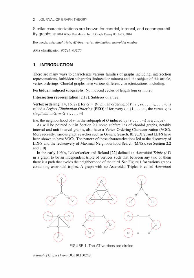
In the early 1960s, Lekkerkerker and Boland [22] defined an Asteroidal Triple (AT)in a graph to be an independent triple of vertices such that between any two of themthere is a path that avoids the neighborhood of the third. See Figure 1 for various graphscontaining asteroidal triples. A graph with no Asteroidal Triples is called Asteroidal

FIGURE 1. The AT vertices are circled.

Journal of Graph Theory DOI 10.1002/jgt

VERTEX ORDERING CHARACTERIZATIONS 3

Triple-free (AT-free), and Lekkerkerker and Boland in [22] showed that a graph is aninterval graph if and only if it is both chordal and AT-free. Starting in the mid 1990s,AT-free graphs have received considerable attention [11] and have been shown to exhibitvarious types of “linear structure.”

In [19], the notion of AT-free graphs was generalized in the following way. Let G bea graph. A set A ⊆ V (G) is asteroidal, if for all a ∈ A, the vertices of A \ {a} belong toone component of G − N[a], where N[a] denotes the closed neighborhood of a, namely{a} together with its (open) neighborhood N(a). The asteroidal number of G, denoted bya(G), is the size of a largest asteroidal set of G. Note that AT-free graphs are the onesthat have asteroidal number at most two.

In this article, we solve the long standing open problem of finding a VOC for AT-freegraphs in particular, and graphs with bounded asteroidal number in general.

1.1. Overview of the Article

In Section 2, we give the required background on VOCs both for subfamilies of AT-freegraphs and for graph searches; we also provide some examples of algorithmic resultsfor these families resulting from graph searches. In Section 3, we present the VOC firstfor AT-free graphs, in particular, and then for graphs of bounded asteroidal number, ingeneral. In both cases the proof is constructive. We then discuss the relationship of thenew VOCs with existing VOCs, as well as whether the AT-free VOC can be attained viastandard graph searches. The article ends with a summary of our contributions and someopen problems.

2. BACKGROUND

If σ is an ordering of the vertices of graph G, we write x <σ y to indicate that x appearsbefore y in the ordering σ . Throughout the article we will assume our graphs are connectedand that n and m, respectively, denote the number of vertices and edges in the graph.We now survey existing results for VOCs both for graph families in the AT-free graphhierarchy and for various graph searches.

2.1. VOCs for Graph Families in the AT-free Graph Hierarchy

First we define various AT-free subfamilies that will be discussed.

� G is an interval graph if it is the intersection graph of intervals of a line (equivalentlysubpaths of a path, thereby showing that interval graphs are chordal); namely, eachvertex represents an interval and two vertices are adjacent if and only if theirintervals intersect.

� G is a unit interval graph if it is an interval graph with an intersection representationby intervals of the same length (equivalent to proper interval graphs where nointerval properly contains another [26]).

� G is a cocomparability graph if its complement G has a transitive orientation ofits edges (i.e. if x → y and y → z then x → z).

It is easy to see that unit interval graphs are strictly contained in interval graphs thatare strictly contained in cocomparability graphs that are strictly contained in AT-free



graphs; consider, respectively, K1,3, C4, C5. The VOCs of these three graph classes are asfollows:

� Unit Interval VOC Theorem [23]: G = (V, E ) is a unit interval graph if and onlyif there is a vertex ordering (VO) σ of V such that for all x <σ y <σ z:

if xz ∈ E, then xy, yz ∈ E. (UI ORDER)

� Interval VOC Theorem [25]: G = (V, E ) is an interval graph if and only if there isa VO σ of V such that for all x <σ y <σ z:

if xz ∈ E, then xy ∈ E. (I ORDER)

� Cocomparability Graph VOC Theorem [21]: G = (V, E ) is a cocomparabilitygraph if and only if there is a VO σ of V such that for all x <σ y <σ z:

if xz ∈ E, then at least one of xy, yz is in E. (COCOMP ORDER)

Chang et al. in [3] generalized cocomparability graphs to k-cocomparability graphsby generalizing the COCOMP ORDER in the following way:

� k-cocomparability Graph VOC Theorem [3]: G = (V, E ) is a k-cocomparabilitygraph if and only if there is a VO σ of V such that for all x <σ y <σ z:

if dist(x, z) ≤ k, then dist(x, y) ≤ k or dist(y, z) ≤ k,

(k-COCOMPORDER)

where dist(·, ·) denotes the distance in G (the length of a shortest path).

Note that cocomparability graphs are precisely the 1-cocomparability graphs. Theyalso proved that AT-Free graphs are strictly contained in 2-cocomparability graphs; strictinclusion is illustrated by the 3-sun (the middle graph in the first row of Fig. 1) whereany ordering of the vertex set is a 2-COCOMP ORDER, since the distance between anytwo vertices is at most two.

The first attempt [9] at a VOC for AT-free graphs extended the COCOMP ORDER inthe following way: consider a vertex ordering σ where for all x <σ y <σ z:

if xz �∈ E, then every x-z path P satisfies N[y] ∩ P �= ∅. (PO ORDER)

The class of graphs (called Path Orderable Graphs) defined by this order strictlycontains cocomparability graphs (consider C5) and is contained in AT-free graphs. It waslater shown that the latter inclusion is also strict (consider the graph in Fig. 2, which is the

8 7

2

1

63

4 5

FIGURE 2. An AT-free graph that is not Path Orderable.



smallest known AT-free graph that is not Path Orderable). To see this, suppose otherwiseand let σ be a PO ORDER of the graph in Figure 2. Then in σ , note that 4 cannot bebetween 1 and 6 because of the path 1, 2, 6 (similarly, 5 cannot be between 1 and 3).Further, the path 8, 7, 5, 6 dictates that 3 is not between 7 and 6, or between 8 and 6, orbetween 7 and 5, which implies that 3 is not between 5 and 6 (similarly, 6 is not between3 and 4). In a similar fashion, the path 3, 4, 5, 6 dictates that 1 is not between 4 and 5.These five restrictions form a cycle showing that σ cannot exist. In [9] it was shown thatrecognizing Path Orderable graphs is NP-complete.

2.2. VOCs for Graph Searches

We begin by introducing Generic Search, first described by Tarjan in the 1970s: start atan arbitrary vertex and at each subsequent stage of the search visit an unvisited vertex thatis adjacent to some previously visited vertex. This produces an ordering of the verticesof the graph, where vertices are listed in the order they are visited by the search. Thisallows us to state a VOC for a graph search X in the form:

“σ , an ordering of V , could be produced by an X search if and only if ....”

We denote this ordering as an X ORDER (i.e. any ordering that could be produced bysearch X). We shall now discuss specific graph searches X. Full descriptions of each ofthe graph searches mentioned in this section appear in [10].

In characterizing various graph searches, we consider a vertex ordering σ produced bythe search and for every a <σ b <σ c such that ac ∈ E but ab /∈ E, we ask:

In the face of the edge ac and the nonedge ab, why is b before c? (see Fig. 3.)

As the results from [10] show, Generic Search, BFS (Breadth-first search) and DFS(Depth-first search) are characterized by the position of a vertex d that is a neighbor ofb. Note that a is a private neighbor of c with respect to b (i.e. ac ∈ E, ab /∈ E).

� Generic Search VOC Theorem: An ordering σ is a Generic Search ORDER ifand only if for all a <σ b <σ c where ac ∈ E, ab /∈ E:

there exists d <σ b such that db ∈ E.

� BFS VOC Theorem: An ordering σ is a BFS ORDER if and only if for alla <σ b <σ c where ac ∈ E, ab /∈ E:

there exists d <σ a such that db ∈ E.

� DFS VOC Theorem: An ordering σ is a DFS ORDER if and only if for alla <σ b <σ c where ac ∈ E, ab /∈ E:

there exists a <σ d <σ b such that db ∈ E.

a b c

FIGURE 3. Ordering of vertices a, b, c.



In the early 1970s, Rose et al. [28] introduced Lexicographic BFS (LBFS) and showedthat an arbitrary LBFS of a graph G is a PEO (perfect elimination ordering) of G if andonly if G is chordal. This was the first linear time recognition algorithm of chordal graphs.LBFS initially assigns a null list to every vertex and then at every iteration chooses anunvisited vertex with the lexicographically largest list. The ith (1 ≤ i < n) chosen vertexappends the label n − i + 1 to the list of each of its unvisited neighbors.

The VOC characterization of LBFS (given below) is similar to the VOC of BFS; theonly difference is that the LBFS VOC requires the vertex d to be a private neighbor ofb, with respect to c. In [10], both Generic Search and DFS are examined where d issimilarly required to be a private neighbor of b, with respect to c. For Generic Search,this results in Maximal Neighbor Search (MNS) where vertex x chosen at a specific stagehas the property that there is no unvisited vertex y where y’s neighborhood in the setof visited vertices strictly contains x’s neighborhood in the set of visited vertices. Theprivate neighbor condition applied to the DFS ordering was shown in [10] to result in agraph search that was named LDFS. It is only recently that applications of LDFS havebeen found as will be briefly discussed in Section 2.3.

The three searches are characterized as follows.

� MNS VOC Theorem: An ordering σ is an MNS ORDER if and only if for alla <σ b <σ c where ac ∈ E, ab /∈ E:

there exists d <σ b such that db ∈ E and dc /∈ E.

� LBFS VOC Theorem [1, 18]: An ordering σ is an LBFS ORDER if and only iffor all a <σ b <σ c where ac ∈ E, ab /∈ E:

there exists d <σ a such that db ∈ E and dc /∈ E.

� LDFS VOC Theorem: An ordering σ is an LDFS ORDER if and only if for alla <σ b <σ c where ac ∈ E, ab /∈ E:

there exists a <σ d <σ b such that db ∈ E and dc /∈ E.

Thus any LBFS and any LDFS ORDER is also an MNS ORDER. In [28] it was shownthat an arbitrary MNS ORDER has the property that it is a PEO if and only if the graphis chordal.1 Thus, as corollaries, this holds not only for LBFS (as remarked earlier), butalso for LDFS and MCS (Maximum Cardinality Search [30]) that starts at an arbitraryvertex and at each subsequent stage chooses a vertex adjacent to the maximum numberof visited vertices.

2.3. Interplay Between These Graph Searches and Graph Families

Applications of graph searches to the various families previously mentioned includerecognition, diameter estimation, and efficient solutions of problems that are NP-completein general. The first, and most celebrated, such recognition algorithm is the previouslymentioned chordal graph recognition algorithm from [28]. More recently it has been

1Interestingly, it seems that the authors of [28] despite discovering the 4-vertexcondition for MNS did not realize that it also characterizes MNS.



5 6

73 4

2

1

FIGURE 4. A graph with an AT {2, 3, 4} that has an LBFS that is an AEO.

shown that unit interval graphs [4] and interval graphs [13] can be recognized by multi-sweep LBFS algorithms using respectively 3 and 6 sweeps. In such multisweep algorithmsit is common for a sweep to be applied in a “+” fashion to a previously obtained vertexordering σ . Under this paradigm when the search has tied vertices and is required tomake a choice, it chooses the rightmost tied vertex in σ . It has also been shown that thelast vertex of an LBFS of graphs in these various families has eccentricity that is withina small constant of the graph’s diameter [1, 6, 15].

In the study of connected AT-free graphs, one of the strongest witnesses of “linearstructure” is the existence of a dominating pair of vertices [11], namely a pair of vertices{x, y} such that every x-y path dominates the graph in the sense that for any such path P,every vertex of the graph is either on P or has a neighbor on P. Vertices 1 and 4 form adominating pair for the graph in Figure 2. In [12], the authors showed that the followingvery simple LBFS algorithm produces such a dominating pair:

1. Let σ be an arbitrary LBFS, and let x be its last vertex.2. Let τ be an arbitrary LBFS that starts at x, and let y be its last vertex.3. Return {x, y}.

Such an application of LBFS outside the chordal graph family was quite unexpectedand produced various LBFS properties of AT-free graphs. In particular, vertices y, zare called unrelated with respect to vertex x if there exist an x-y path P that is outsidez’s neighborhood and an x-z path Q that is outside y’s neighborhood. For the graph inFigure 2, the vertices 1 and 4 are unrelated with respect to the vertex 6 because of thepaths 6, 2, 1 and 6, 5, 4. Vertex x is called admissible if no pair of vertices is unrelatedwith respect to x.

Admissible elimination: For G = (V, E ), an ordering of V : v1, v2, . . . , vi, . . . , vn

is called an Admissible Elimination Ordering (AEO) if for every i ∈ {1, . . . , n},the vertex vi is admissible in Gi = G[v1, . . . , vi].

Similar to the theorem of Rose et al. [28] that an arbitrary LBFS of a chordal graphis a PEO, it was shown in [12] that an arbitrary LBFS of an AT-free graph is an AEO.Unfortunately, the converse is not true, as shown by the graph in Figure 4 (with AT{2, 3, 4}), where the LBFS 1 2 3 4 5 6 7 is an AEO. However, it was shown in [8] that agraph G is AT-free if and only if every LBFS of G is an AEO.

As mentioned in the previous subsection, LDFS was discovered by applying the privateneighbor requirement to the vertex d in the DFS VOC, and only recently have applicationsof LDFS been discovered. In particular, a cocomparability graph has a COCOMP orderthat is also an LDFS and on such an order, some very simple greedy algorithms that work



for interval graphs, also work for cocomparability graphs. This happens for the minimumpath cover problem [5], the longest path problem [24], and the maximum independentset and minimum clique cover problems [7]. Furthermore, by doing a direct translationof the minimum path cover algorithm to the associated poset, one has a simple certifyingalgorithm for the bump number problem of posets [5].

3. RESULTS

We now proceed to the main results of the article. Since the result for AT-freegraphs is easier to state and prove (and will be of greater interest to some read-ers), we will first concentrate on AT-free graphs and then generalize the result tographs of bounded asteroidal number. The structure of this section is as follows.In the next two subsections, we introduce some useful tools and notation, and thenseparately discuss a VOC for AT-free graphs and graphs of bounded asteroidalnumber.

3.1 Lexicographic Ordering

To construct the orderings we shall select vertices based on special vectors that weassign to the vertices. We compare these vectors using the lexicographic (dictionary)ordering. To make our arguments clearer (and more precise), we briefly discuss someuseful properties of lexicographic orderings.

We use the lexicographic ordering on sequences of integers defined as follows.

Definition 1. Let a1, . . . , as and b1, . . . , bt be two sequences of integers. Let i be thelargest index such that i ≤ min{s, t} and a1 = b1, a2 = b2, . . . , ai = bi; if a1 �= b1, thendefine i as 0.

We write (a1, . . . , as) ≺ (b1, . . . , bt ) and say that the sequence a1, . . . , as is lexico-graphically smaller than b1, . . . , bt if i < t and either i = s or ai+1 < bi+1.

We write (a1, . . . , as) � (b1, . . . , bt ) if either (a1, . . . , as) ≺ (b1, . . . , bt ) or the twosequences are identical.

For instance (1, 3, 1) ≺ (1, 3, 1, 2) ≺ (1, 3, 2) ≺ (2, 1) ≺ (3), where (3) is lexico-graphically largest among these sequences. Note that ≺ is a total order. We shall needthe following straightforward observations.

Lemma 2. Let a1, . . . , as and b1, . . . , bt be two sequences of integers. If there existsj ≤ min{s, t} such that (a1, . . . , a j) ≺ (b1, . . . , b j), then (a1, . . . , as) ≺ (b1, . . . , bt ).

Proof. Consider the largest i ≤ j such that a1 = b1, . . . , ai = bi. Since (a1, . . . ,

a j) ≺ (b1, . . . , b j), we have i < j and ai+1 < bi+1 by definition. So, since j ≤ min{s, t},we deduce i < t and i �= s. Thus (a1, . . . , as) ≺ (b1, . . . , bt ) by definition. �Lemma 3. Suppose that b1 ≥ b2 ≥ . . . ≥ bt and let f1, . . . , fs be distinct integers from{1, . . . , t}. Then (b f1, b f2, . . . , b fs ) � (b1, . . . , bt ).

For example consider b1 = 5 ≥ b2 = 5 ≥ b3 = 3 ≥ b4 = 2 ≥ b5 = 2 ≥ b6 = 1. Withf1 = 1, f2 = 3, f3 = 4, f4 = 2, f5 = 6, we see that (b f1, · · · , b fs ) is (5, 3, 2, 5, 1) andalso that (5, 3, 2, 5, 1) ≺ (5, 5, 3, 2, 2, 1).



8 7

2

1

63

4 5

comp(1) = (6)comp(2) = (2)comp(3) = (4, 1)comp(4) = (4)comp(5) = (4)comp(6) = (4, 1)comp(7) = (2, 1, 1)comp(8) = (2, 1, 1)

8 7

2

1

63

4 5

comp(1) = (6)comp(2) = (2)comp(3) = (4, 1)comp(4) = (4)comp(5) = (4)comp(6) = (4, 1)comp(7) = (2, 1, 1)comp(8) = (2, 1, 1)

FIGURE 5. The graph from Figure 2 and its comp vectors.

Proof. Since f1, . . . , fs are distinct, the mapping f : i �→ fi is injective. Thus s ≤ t.Let i ≤ s be the largest index such that b f1 = b1, b f2 = b2, . . . , b fi = bi; if b f1 �= b1,

then let i = 0. If i = s < t, then (b f1, . . . , b fs ) ≺ (b1, . . . , bt ) by definition. If i = s = t,then the two sequences are actually identical, since f is injective. Thus (b f1, . . . , b fs ) �(b1, . . . , bt ) when i = s. So we may assume i < s.

Let A = { j | b j > bi+1}. We now show that A ⊆ { f j | 1 ≤ j ≤ i}. Since b1 ≥ b2 ≥. . . ≥ bt , we have A ⊆ {1, . . . , i}. Moreover, since b1 = b f1 , b2 = b f2, . . . , bi = b fi , weconclude that { f j | j ∈ A} ⊆ A. In other words, f (A) ⊆ A and since f is injective, we findthat f (A) = A. Thus A = { f j | j ∈ A} ⊆ { f j | 1 ≤ j ≤ i}.

From this, we now deduce that b f j ≤ bi+1 for all j > i. Since b fi+1 �= bi+1, we concludeb fi+1 < bi+1 which yields (b f1, b f2, . . . , b fs ) � (b1, . . . , bt ), as required. �

3.2. Components of the Non-neighborhood

In order to deal with asteroidal sets, we need a way to handle the structure of thenonneighborhoods of vertices of G. For this purpose, we assign to every vertex v of G avector comp(v) defined as follows.

Definition 4. Let v be a vertex of G, and letC1,C2, . . . ,Ct be the connected componentsof G − N[v] where |C1| ≥ |C2| ≥ . . . ≥ |Ct |. Then define

comp(v) = (|C1|, |C2|, . . . , |Ct |).The comp vectors for the graph from Figure 2 are presented as Figure 5. Note that the

comp vectors are sequences of integers. Thus we can compare them lexicographicallyusing the relations ≺ and � as defined earlier. In particular, we can define the followingordering of the vertices of G.

Definition 5. An ordering v1, v2, · · · , vn of the vertices of a graph G is called aLEXCOMP ORDER if comp(vi) � comp(vi+1) for all 1 ≤ i < n.

As an example, for the graph in Figure 5, the LEXCOMP ORDERs can be representedas 2 [7 8][4 5][3 6] 1, where the square brackets indicate that choice could be made. Astraightforward BFS algorithm computes a LEXCOMP ORDER of a given graph in timeO(n × m); recall that our graphs are assumed to be connected.

As will be seen in the next two subsections, LEXCOMP ORDERs play a critical role inour vertex order characterizations of AT-free graphs in particular, and graphs of boundedasteroidal number in general. The main useful feature of the comp vectors is presentedin the following lemma.



Lemma 6. Let v be a vertex of G and let C1,C2, . . . ,Ct be the connected components ofG − N[v] where |C1| ≥ |C2| ≥ . . . ≥ |Ct |. Then for every i ∈ {1, . . . , t} and every x ∈ Ci

such that comp(x) � comp(v), each of C1, . . . ,Ci−1 is also a connected component ofG − N[x].

Proof. Suppose that the claim fails for some i ∈ {1, . . . , t} and x ∈ Ci such thatcomp(x) � comp(v). In other words, there exists j < i such that the set Cj is not aconnected component of G − N[x]. Choose j to be smallest with this property.

Since x ∈ Ci and j < i, the vertex x is neither in Cj nor has a neighbor in Cj. (Notethat C1, . . . ,Ct are distinct connected components.) So Cj induces a connected subgraphin G − N[x]. But Cj itself is not a connected component of G − N[x]. Therefore, thereexists a connected component D of G − N[x] that properly contains Cj. Thus |Cj| < |D|implying (|C1|, . . . , |Cj−1|, |Cj|) ≺ (|C1|, . . . , |Cj−1|, |D|). From this, by Lemma 2, weobtain comp(v) = (|C1|, . . . , |Ct |) ≺ (|C1|, . . . , |Cj−1|, |D|).

Moreover, the minimality of j implies that C1, . . . ,Cj−1 are connected components ofG − N[x]. Thus D is not one ofC1, . . . ,Cj−1, since it contains Cj but none of C1, . . . ,Cj−1

could since C1, . . . ,Cj are distinct connected components of G − N[v]. In other words,C1, . . . ,Cj−1, D are distinct connected components of G − N[x]. So Lemma 3 and thedefinition of comp(x) produce (|C1|, . . . , |Cj−1|, |D|) � comp(x).

Putting the two together gives us comp(v) ≺ comp(x), a contradiction. �

3.3. AT-free Graphs

We can now proceed to the main theorems. Recall that nonadjacent vertices x, y areunrelated in a graph G with respect to a vertex z if there exists an x-z path in G − N[y]and an y-z path in G − N[x].

We write I(x, y) to denote the set of all z such that x and y are unrelated in G withrespect to z. Note that I(x, y) = I(y, x).

For the graph in Figure 2; the nonempty I-sets for this graph are: I(1, 4) = I(4, 1) ={6, 7}; I(1, 5) = I(5, 1) = {3, 8}; I(3, 5) = I(5, 3) = {8}; I(3, 6) = I(6, 3) = {7, 8};I(4, 6) = I(6, 4) = {7}.

In a related fashion, we write J (z) to denote the set of all unordered pairs {x, y} suchthat z ∈ I(x, y). (In other words, J (z) contains the pairs of vertices that are unrelatedwith respect to z.)

For the graph in Figure 2, the nonempty J -sets are: J (3) = {{1, 5}}; J (6) = {{1, 4}};J (7) = {{1, 4}, {3, 6}, {4, 6}}; J (8) = {{1, 5}, {3, 5}, {3, 6}}. Observe that if A is anasteroidal set of size greater than two, then for all z ∈ A, every pair of vertices fromA \ {z} is in J (z).

Using this notation, we define an ordering of G as follows.

Definition 7. An ordering σ of the vertices of G is an AT-free ORDER if every vertexz and every pair {x, y} ∈ J (z) is such that z <σ x or z <σ y.

Before proving the VOC theorem for AT-free graphs it is worth noting the differencebetween an AT-free ORDER and an AEO (Admissible Elimination Ordering – see Section2.3). An AEO forbids a vertex z having an unrelated pair {x, y} where all vertices of thez-x and z-y paths are before z in the ordering. On the other hand, an AT-free ORDERforbids a vertex z having an unrelated pair {x, y} where x and y are before z in the ordering;note, there is no restriction on the location of the interior vertices of the z-x and z-y paths.



{6, 7} {7}

{7, 8}

{8}

{3, 8}1

4

6

35

2

7

8

FIGURE 6. The unrelated pairs graph for the graph in Figure 2.

What now follows is the VOC theorem for AT-free graphs.

Theorem 8. G is AT-free if and only if G admits an AT-free ORDER.

Proof. For the backward direction, suppose that σ is an AT-free ORDER of G, but Gcontains an asteroidal triple {x, y, z}. By symmetry, we may assume x <σ y <σ z. Since{x, y, z} is an asteroidal triple in G, there exists an x-z path in G − N[y] and also a y-zpath in G − N[x]. From this, we deduce that {x, y} ∈ J (z). However x <σ z and y <σ zcontradicting our assumption that σ is an AT-free ORDER.

For the converse, we define the unrelated pairs graph H as follows:

(i) V (H) = V (G),(ii) E(H) = {(x, y) | I(x, y) �= ∅},

(iii) Each edge e = (x, y) ∈ E(H) is assigned the label label(e) = I(x, y).

Note that the label on an edge (x, y) of H contains all vertices z where z is unrelatedto {x, y}. The unrelated pairs graph H for the graph in Figure 2 appears as Figure 6.

The converse is a consequence of the following claim.

Claim 1. If G is AT-free, then in every induced subgraph H ′ of H, there exists a vertexz ∈ V (H ′) such that every e ∈ E(H ′) satisfies z /∈ label(e). In particular, a vertex inV (H ′) of largest comp vector has this property.

In other words, we claim that H ′ contains a vertex z that does not appear in the labelof any edge of H ′. To prove this, we choose z to be a vertex of H ′ with lexicographicallylargest value of comp(z) among the vertices of H ′. We show that no edge of H ′ has z inits label which will prove the claim.

Suppose otherwise, and let e = (x, y) be an edge of H ′ with z ∈ label(e). Since H ′ isan induced subgraph of H, we deduce e ∈ E(H). Thus {x, y} ∈ J (z). This means thatthere exists an x-z path in G − N[y] and also a y-z path in G − N[x]. In particular, both xand y are vertices in G − N[z].

Let C1, . . . ,Ct be the connected components of G − N[z] where |C1| ≥ |C2| ≥ . . . ≥|Ct |. Recall that comp(z) = (|C1|, . . . , |Ct |). Since x, y are vertices in G − N[z], thereexist indices i, j such that x ∈ Ci and y ∈ Cj.

Suppose first that i = j. Then we claim that {x, y, z} is an AT in G. Indeed, recall thatthere exists a y-z path in G − N[x], and also an x-z path in G − N[y]. The remaining x-ypath in G − N[z] is provided by walking from x to y in Ci = Cj. Since G is assumed tobe AT-free, this is impossible, and we conclude i �= j.



By symmetry, we may assume that j < i. Recall that z was chosen to have lexicograph-ically largest comp(z) among the vertices of H ′. Note that x ∈ V (H ′), since e = (x, y) isan edge of H ′. Thus comp(x) � comp(z) and by Lemma 6, each of C1, . . . ,Ci−1 is a con-nected component in G − N[x]. In particular, Cj is a connected component of G − N[x],since j < i. However, this is impossible. Recall that y ∈ Cj and that there exists a y-z pathP in G − N[x]. Thus z ∈ Cj which contradicts the fact that Cj is a connected componentof G − N[z]. This proves Claim 1.

We construct the required ordering σ of V (G) using the following algorithm.

Input: a graph G = (V, E )

Output:ordering σ = σ (1), σ (2), . . . , σ (n) of the vertices of Gconstruct the unrelated pairs graph Hinitialize H ′ ← Hfor i = |V | downto 1 do∣∣∣∣∣∣

pick a vertex v of H ′ that has largest comp vector among all vertices of H ′ (�)

σ (i) ← vremove v from H ′

end for

Clearly, the ordering σ is well defined. We now verify that σ is an AT-free ORDER.Let z ∈ V (G), let {x, y} ∈ J (z), and consider the edge e = (x, y) ∈ H. The definition

of H implies that z ∈ label(e). Consider the graph H ′ in the algorithm when z is chosenby rule (�). By Claim 1, this choice means that z is not in the label of any edge of H ′.Therefore, e is not an edge of H ′. Since H ′ is an induced subgraph of H, this impliesthat at least one of x, y is not a vertex of H ′, namely, x or y was removed earlier in thealgorithm. In other words, z <σ x or z <σ y as required.

This proves that σ is an AT-free ORDER of G which concludes the proof. �As a consequence of the proof (namely Claim 1), we obtain the following strengthening.

Corollary 9. A graph G is AT-free if and only if an arbitrary LEXCOMP ORDER ofG is an AT-free ORDER.

For the graph in Figure 5, the LEXCOMP ORDERs are 2 [7 8][4 5][3 6] 1, where thesquare brackets indicate that choice could be made. These, however, are not the onlyAT-free ORDERs of this graph; consider for instance the order 1 3 2 8 5 7 6 4.

3.4. Graphs with Bounded Asteroidal Number

We now generalize the AT-free ORDER and the VOC proof to graphs of boundedasteroidal number k ≥ 2. We define a k-asteroidal ORDER and prove that it characterizesgraphs of asteroidal number at most k.

The proof of this will follow essentially the same steps as the VOC proof for the AT-free ORDER (from the previous section), with only a few minor differences. Namely, inplace of the unrelated pairs graph, we will now consider sets of unrelated pairs and use thecorresponding hypergraph in the elimination process. The process will again be guidedby the same comp vectors that will again be chosen in non-increasing lexicographic order.In the remainder, we shall assume that k ≥ 2 is a fixed integer.



As before, for nonadjacent vertices x, y of G, we let I(x, y) denote the set of all z suchthat x and y are unrelated with respect to z.

For a vertex z, we let Jk(z) denote the collection of all independent sets S ⊆ V (G) with|S| = k such that z ∈ I(x, y) for all x, y ∈ S. That is, Jk(z) contains all sets of cardinalityk in which every pair of vertices is unrelated with respect to z. Observe that if A is anasteroidal set of size k + 1, then A \ {z} ∈ Jk(z) for all z ∈ A.

Definition 10. An ordering σ of the vertices of G is a k-asteroidal ORDER if forevery vertex z and set S ∈ Jk(z) there exists x ∈ S with z <σ x.

Recall that a(G) denotes the size of a largest asteroidal set in G.

Theorem 11. a(G) ≤ k if and only if G admits a k-asteroidal ORDER.

Proof. For the backward direction, suppose that σ is a k-asteroidal ORDER of G,but G contains an asteroidal set A of size k + 1. (Note that if G contains a larger asteroidalset, then any k + 1 subset of it is also asteroidal.) Let z be the last vertex of A in σ , that is, zsatisfies x <σ z for all x ∈ A \ {z}. Clearly, A \ {z} ∈ Jk(z). But x <σ z for all x ∈ A \ {z}contradicting our assumption that σ is a k-asteroidal ORDER.

For the converse, we define the unrelated pairs hypergraph H as follows:

(i) V (H) = V (G),(ii) E(H) = {S ⊆ V (G) | ∃z ∈ V (G) such that S ∈ Jk(z)},

(iii) Each edge e = S ∈ E(H) is assigned the label label(e) = {z∣∣ S ∈ Jk(z)

}.

The converse is a consequence of the following claim.

Claim 2. If a(G) ≤ k, then in every induced subhypergraph H′ of H, there exists avertex z ∈ V (H′) such that every e ∈ E(H′) satisfies z /∈ label(e). In particular, a vertexin V (H′) of largest comp vector has this property.

In other words, we claim that H′ contains a vertex z that does not appear in the labelof any edge of H′. Note that for a set X ⊆ V (H), we say that H′ is the subhypergraph ofH induced on X if V (H′) = X and E(H′) = {S ∈ E(H) | S ⊆ X}.

To prove Claim 2, we let z be a vertex of H′ with lexicographically largest value ofcomp(z) among the vertices of H′. We show that no edge of H′ has z in its label.

Suppose otherwise, and let e = S be an edge of H′ with z ∈ label(e). Since H′ is aninduced subgraph ofH, we have e ∈ E(H), and thus S ∈ Jk(z). In particular, every vertexin S is a vertex of G − N[z]. Let C1, . . . ,Ct be the connected components of G − N[z]where |C1| ≥ |C2| ≥ . . . ≥ |Ct |. Note that S ⊆ C1 ∪ · · · ∪ Ct . Thus, since S is non-empty,let i be the largest index such that Ci ∩ S �= ∅.

Suppose first that S ⊆ Ci. Then S ∪ {z} is an asteroidal set of G. To see this, we need toverify that for every u ∈ S ∪ {z}, the vertices in S ∪ {z} \ {u} belong to the same connectedcomponent of G − N[u]. If u = z, then this is clear, since S ⊆ Ci. For u �= z, note thatz ∈ I(x, u) and z ∈ I(y, u) for all x, y ∈ S \ {u}, since S ∈ Jk(z). Thus there exists anx-z path in G − N[u], and also a y-z path in G − N[u]. Using these paths we can movefrom x to z to y in G − N[u]. This shows that all vertices in S ∪ {z} \ {u} belong to thesame connected component of G − N[u]. Thus S ∪ {z} is indeed an asteroidal set of G.However, |S ∪ {z}| = k + 1 and we assume a(G) ≤ k.

Thus we deduce S �⊆ Ci. In particular, there exists y ∈ S \ Ci and also x ∈ S ∩ Ci,since S ∩ Ci �= ∅. The maximality of i implies that y ∈ Cj for some j < i. Recall that zwas chosen to have lexicographically largest comp(z) among the vertices of H′. Note



that x ∈ S ⊆ V (H′), since e = S is an edge of H′. Thus comp(x) � comp(z) and byLemma 6, we deduce that Cj is a connected component of G − N[x], since j < i. Notethat y ∈ Cj and z ∈ I(x, y), since {x, y} ⊆ S ∈ Jk(z). This implies that there exists ay-z path P in G − N[x]. Thus z ∈ Cj which contradicts the fact that Cj is a connectedcomponent of G − N[z]. This concludes the proof of Claim 2.

We now construct the required ordering σ of V (G) using the following algorithm.

Input: a graph G = (V, E )

Output: ordering σ = σ (1), σ (2), . . . , σ (n) of the vertices of Gconstruct the unrelated pairs hypergraph Hinitialize H′ ← Hfor i = |V | downto 1∣∣∣∣∣∣

pick a vertex v of H′ that has the largest comp vector among all vertices of H′ (�)

σ (i) ← vremove v and all hyperedges of H′ containing v from H′

end for

Clearly, the ordering σ is well-defined. Let us now verify that σ is a k-asteroidalORDER. Let z ∈ V (G), let S ∈ Jk(z), and consider the edge e = S ∈ E(H). By thedefinition of H, we have z ∈ label(e). Consider the hypergraph H′ in the algorithm whenz is chosen by rule (�). By Claim 2, this means that z is not in the label of any edge of H′.Therefore, e is not an edge of H′. Since H′ is an induced subhypergraph of H, there mustexist x ∈ S with x �∈ V (H′). That is, x was removed earlier in the algorithm implyingz <σ x.

This proves that σ is a k-asteroidal ORDER of G which concludes the proof. �

As a consequence of the proof (namely Claim 2), we obtain the following strengthening.

Corollary 12. A graph G has asteroidal number at most k if and only if an arbitraryLEXCOMP ORDER of G is a k-asteroidal ORDER of G.

4. DISCUSSION

In this section, we examine the previous results from two perspectives. Firstly we observehow our results produce a hierarchy of VOCs that captures all graphs, and secondly weask whether the AT-free ORDER can be achieved by traditional graph searches.

4.1. Hierarchy of VOCs

First, we note that it is easy to show that a PO ORDER is an AT-free ORDER, and thusso are a COCOMP ORDER, an I ORDER and a UI ORDER. Indeed, suppose that σ is aPO ORDER of a graph G = (V, E ), but it is not an AT-free ORDER of G. Thus there arevertices z and x, y such that z ∈ I(x, y) and {x, y} <σ z. By symmetry, we may assumethat x <σ y <σ z. Since z ∈ I(x, y), there exists an x-z path P in G − N[y]. Namely, wehave N[y] ∩ P = ∅. However, note that xz �∈ E. Thus the vertices x <σ y <σ z violate thedefinition of a PO ORDER for the path P. So no such vertices exist that shows that σ



1

2 3 4 5 6 7 8 9

10 11

12

13 14 15 16 17 18 19 20

21 22

FIGURE 7. “Two cupcakes”: no AT-free order is also an LBFS.

is indeed an AT-free ORDER. In a similar manner, one can show that every k-asteroidalORDER is also a (k + 1)-asteroidal ORDER. Thus starting with UI ORDER, we havean infinite hierarchy of vertex orderings:

UI ⊂ I ⊂ COCOMP ⊂ PO ⊂ AT-free ⊂ 3-asteroidal ⊂ . . . ⊂ k-asteroidal ⊂ . . .

Note that every graph admits at least one of these orderings (since every graph has aspecific asteroidal number).

4.2. Graph Searches and AT-free ORDERs

As seen in the two previous corollaries, the LEXCOMP ORDER plays a key role infinding constructive proofs of the VOCs of AT-free graphs and graphs of boundedasteroidal number. Although a LEXCOMP ORDER is a graph search in the sense thatevery vertex is visited, it is not necessarily a Generic Search ORDER as illustrated by a C4

where we start with two nonadjacent vertices. This raises the question of whether everyAT-free graph admits an AT-free ORDER that is a particular traditional graph search (asdescribed in Section 2.2).

Recall first that an MNS of a chordal graph is always a PEO. Similarly, an LBFS ofan AT-free graph is always an AEO. It would be useful if a similar statement could beshown for AT-free ORDER. However, as we will see shortly, this is not the case. Fromanother perspective, we mentioned earlier that every cocomparability graph admits aCOCOMP ORDER that is also an LDFS. In particular, a simple LDFS+ of a COCOMPORDER yields such an order. This property turned out to be immensely useful in recentalgorithmic results on cocomparability graphs [5,7,24]. It again would seem useful if thiscarried over to AT-free ORDERs. Alas, this is not the case. Not only does the + techniquefail (or several sweeps of + searches), but actually there are AT-free graphs where noLBFS, LDFS, or even DFS is also an AT-free ORDER. We now discuss examples ofsuch graphs.

To see that there are AT-free graphs where no DFS can be an AT-free ORDER, considertwo C5s that share a vertex (the “center vertex”). Suppose that σ is a DFS and also anAT-free ORDER of this graph. The first vertex in σ other than the center belongs to oneof the two C5s. In the other C5, there are two neighbors of the center; the rightmost of thetwo (in σ ) violates the definition of an AT-free ORDER.

We now discuss the graph shown in Figure 7 and show that no LBFS of it canbe an AT-free ORDER. The graph has 22 vertices and consists of two identical partscalled “cupcakes” on vertices {1, . . . , 11} and {12, . . . , 22}. Each part admits further



symmetries: vertices {2, 3, 4, 5, 10} and {6, 7, 8, 9, 11} can exchange labels, vertices 2, 3can exchange labels with 5, 4, respectively, and similarly 6, 7 can exchange labels with9, 8, respectively. We shall use these symmetries in our analysis below.

We now show that this graph does not admit an LBFS that is also an AT-free ORDER.Assume that σ is such an order, where by symmetry 12 <σ 1. Since σ is an LBFS, itfollows that 1 <σ {2, . . . , 9} <σ {10, 11}. In particular, either {2, 3, 4, 5} <σ {6, 7, 8, 9}or {6, 7, 8, 9} <σ {2, 3, 4, 5}. By symmetry, assume the former. Then note that 9 <σ 7and 6 <σ 8, since 9 ∈ I(2, 7) and 6 ∈ I(2, 8). So either 6 <σ {7, 8, 9} or 9 <σ {6, 7, 8}.Again, by symmetry, we shall assume that 6 <σ {7, 8, 9}. Then it follows that 7 <σ {8, 9},because σ is an LBFS and 1 <σ {2, . . . , 9} <σ {10, 11}. But then 7 <σ 9, a contradiction.

Although these results are somewhat disappointing, there may be other ways of gener-ating vertex orderings that are AT-free ORDERs. In particular, we conjecture that everyAT-free graph has a BFS that is an AT-free ORDER. Furthermore, perhaps there existsa graph search whose reversal is an AT-free ORDER. As examples, note that the graphin Figure 7 admits a BFS that is also an AT-free order. It also admits a BFS and a DFSwhose reversals are AT-free orders. These are as follows:

both a BFS and an AT-free ORDER:1 2 5 6 9 3 4 7 8 12 10 11 13 16 17 20 14 15 18 19 21 22

a BFS whose reversal is an AT-free ORDER:10 11 3 4 2 5 6 9 7 8 1 12 14 15 13 16 17 18 19 20 21 22

a DFS whose reversal is an AT-free ORDER:11 10 3 4 5 1 2 6 7 8 9 12 14 15 16 22 13 21 17 18 19 20

However, no LBFS, no LDFS, and in fact, no MNS of the graph in Figure 7 is areversal of an AT-free ORDER. Indeed, suppose that σ is such an order. Note that thelast vertex of an AT-free order is always admissible. The graph in Figure 7 has only 4admissible vertices, namely 10, 11, 21, and 22. Since σ is a reversal of an AT-free order,one of these four vertices is the first vertex in σ . By symmetry, we may assume that 10is first in σ . Thus the second vertex in σ must be a neighbor of 10. It cannot be 3 or 4,since {3, 4} ⊆ I(11, 12) and neither 11 nor 12 has been visited yet. It also cannot be 2,5, 6, or 9, since {2, 9} ⊆ I(4, 7) and {5, 6} ⊆ I(3, 8). Thus the second vertex in σ mustbe 11. Now, because σ is an MNS, the third vertex in σ is one of 2, 5, 6, 9. But this isimpossible, since again {2, 9} ⊆ I(4, 7) and {5, 6} ⊆ I(3, 8).

5. CONCLUDING REMARKS

As the main result of this article, we have described and proved a Vertex OrderingCharacterization (VOC) for AT-free graphs (the first VOC for this class) and also VOCsfor graphs of bounded asteroidal number in general. Even though our VOC theorem bringsus closer to understanding AT-free graphs, further research is still needed to obtain usefulstructural tools for AT-free graphs with (hopefully) nice algorithmic consequences. It isnoteworthy that the LEXCOMP ORDER provides such an AT-free VOC. Perhaps themost important questions resulting from our work are:

Question 1. What structure of AT-free graphs is revealed through the LEXCOMPORDER?



Question 2. Can the LEXCOMP ORDER be used to develop polynomial time algo-rithms for the open problems on AT-free graphs listed below?

Question 3. Can the LEXCOMP ORDER be of any use in understanding the structureof other families of graphs?

As shown in Section 4.2, we cannot expect an AT-free ORDER to have nice propertiessuch as being an LBFS or LDFS or even a DFS. However, there are still some possibilitiesleft. We summarize them as follows:

Question 4. Does every AT-free graph admit an AT-free ORDER that is also a BFS?

Question 5. Does every AT-free graph admit an AT-free ORDER whose reversal is aDFS?

In fact, we can ask even more generally.

Question 6. Does every AT-free graph admit an AT-free ORDER that is, or whosereversal is, a Generic Search ORDER?

Finally, the following are longstanding open questions on AT-free graphs which havenot yet been examined from the structural perspective.

Question 7. What is the complexity of colouring in AT-free graphs?

Question 8. What is the complexity status of all Hamiltonian problems on AT-freegraphs?

Note that the complexity of k-coloring in AT-free graphs for every fixed k has alreadybeen resolved [20,29]. However, the general question (for unbounded k) as well as allHamiltonian problems remain challenging open problems.

ACKNOWLEDGMENT

The authors wish to thank the Natural Sciences and Engineering Research Council forfinancial support and the two anonymous referees for their helpful suggestions.

REFERENCES

[1] A. Brandstadt, F. F. Dragan, and F. Nicolai, LexBFS-orderings and powers ofchordal graphs, Discrete Math 171 (1997), 27–42.

[2] P. Buneman, A characterization of rigid circuit graphs, Discrete Math 9(1974), 205–212.

[3] J. M. Chang, C. W. Ho, and M. T. Ko, Powers of asteroidal triple free graphswith applications, Ars Combinatoria 67 (2003), 161–173.

[4] D. G. Corneil, A simple 3-sweep LBFS algorithm for the recognition of unitinterval graphs, Discrete Appl Math 138 (2004), 371–379.

[5] D. G. Corneil, B. Dalton, and M. Habib, LDFS-based certifying algorithmfor the minimum path cover problem on cocomparability graphs, SIAM JComput 42 (2013), 792–807.

[6] D. G. Corneil, F. Dragan, M. Habib, and C. Paul, Diameter determination onrestricted graph families, Discrete Appl Math 113 (2001), 143–166.



[7] D. G. Corneil, J. Dusart, M. Habib, and E. Kohler, On the power of graphsearching for cocomparability graphs, (2013), manuscript.

[8] D. G. Corneil and E. Kohler, (2012), unpublished manuscript.[9] D. G. Corneil, E. Kohler, S. Olariu, and L. Stewart, On subfamilies of AT-free

graphs, SIAM J Discrete Math 20 (2006), 105–118.[10] D. G. Corneil and R. Krueger, A unified view of graph searching, SIAM J

Discrete Math 22 (2008), 1259–1276.[11] D. G. Corneil, S. Olariu, and L. Stewart, Asteroidal triple-free graphs, SIAM

J Discrete Math 10 (1997), 399–430.[12] D. G. Corneil, S. Olariu, and L. Stewart, Linear time algorithms for dom-

inating pairs in asteroidal triple-free graphs, SIAM J Comput 28 (1999),1284–1297.

[13] D. G. Corneil, S. Olariu, and L. Stewart, The LBFS structure and recognitionof interval graphs, SIAM J Discrete Math 23 (2009), 1905–1953.

[14] G. Dirac, On rigid circuit graphs, Abhandlungen aus dem MathematischenSeminar der Universitat Hamburg 25 (1961), 71–76.

[15] F. F. Dragan, Almost diameter of a house-hole-free graph via LexBFS, Dis-crete Appl Math 95 (1999), 223–239.

[16] D. R. Fulkerson and O. A. Gross, Incidence matrices and interval graphs,Pacific J Math 15 (1965), 120–132.

[17] F. Gavril, The intersection graphs of subtrees in trees are exactly the chordalgraphs, J Combin Theory B 16 (1974), 47–56.

[18] M. C. Golumbic, Algorithmic Graph Theory and Perfect Graphs, 2nd edn.,Annals of Discrete Mathematics, vol. 57, Elsevier, Amsterdam, 2004.

[19] T. Kloks, D. Kratsch, and H. Muller, Asteroidal sets in graphs, Graph The-oretic Concepts in Computer Science (WG’97), Lecture Notes in ComputerScience 1335, Springer-Verlag, Berlin, 1997, pp. 229–241.

[20] D. Kratsch and H. Muller, Colouring AT-free graphs, ESA 2012, LectureNotes in Computer Science 7501, Springer-Verlag, Berlin, 2012, pp. 707–718.

[21] D. Kratsch and L. Stewart, Domination on cocomparability graphs, SIAM JDiscrete Math 6 (1993), 400–417.

[22] C. G. Lekkerkerker and J. C. Boland, Representation of a finite graph by a setof intervals on the real line, Fundamenta Mathematicae 51 (1962), 45–64.

[23] P. J. Looges and S. Olariu, Optimal greedy algorithms for indifference graphs,Comput Math Appl 25 (1993), 15–25.

[24] G. B. Mertzios and D. G. Corneil, A simple polynomial time algorithm forthe longest path problem on cocomparability graphs, SIAM J Discrete Math26 (2012), 940–963.

[25] S. Olariu, An optimal greedy heuristic to color interval graphs, InformationProcessing Lett 37 (1991), 65–80.

[26] F. S. Roberts, Indifference graphs, Proof Techniques in Graph Theory (F.Harary, Ed.), Academic Press, New York, 1969, pp. 139–146.



[27] D. J. Rose, Triangulated graphs and the elimination process, J Math AnalAppl 32 (1970), 597–609.

[28] D. J. Rose, R. E. Tarjan, and G. S. Lueker, Algorithmic aspects of vertexelimination on graphs, SIAM J Comput 5 (1976), 266–283.

[29] J. Stacho, 3-colouring AT-free graphs in polynomial time, Algorithmica 64(2012), 384–399.

[30] R. E. Tarjan and M. Yannakakis, Simple linear time algorithms to test chordal-ity of graphs, test acyclicity of hypergraphs, and selectively reduce acyclichypergraphs, SIAM J Comput 13 (1984), 566–579.


Documents

Vertex Ordering Characterizations of Graphs of Bounded Asteroidal Number