Version 1.7 Oberlain Jiaen Frédéric Nteukam T. Ren · PDF fileArticle 45 of the Solvency II Directive sets the rules ... taking into account all the contractual obligations that

PUBLIC - 1

INTERNAL MODEL IN LIFE INSURANCE: APPLICATION OF LEAST SQUARES MONTE CARLO

IN RISK ASSESSMENT

Version 1.7

Oberlain

Nteukam T.

Jiaen

Ren

Frédéric

Planchet

Université de Lyon - Université Claude Bernard Lyon 1

ISFA – Actuarial School

HSBC Assurances - General Risk Assessment and Asset Liability Management

Abstract

In this paper we show how prospective modelling of an economic balance sheet using the least squares

Monte Carlo (LSMC) approach can be implemented in practice. The first aim is to review the

convergence properties of the LSMC estimator in the context of life assurance. We pay particular

attention to the practicalities of implementing such a technique in the real world. The paper also presents

some examples of using the valuation function calibrated in this way.

KEYWORDS: Solvency II, Economic capital, Economic balance sheet, risk management, risk appetite,

life insurance, stochastic models, least squares Monte Carlo

Acknowledgment : The authors warmly thanks the anonymous referee for valuable comments and

suggestions improving the first version of this paper.

Contact: [email protected] Corresponding author. Contact: [email protected] Institut de Science Financière et d’Assurances (ISFA) - 50 avenue Tony Garnier - 69366 Lyon Cedex 07 –

France. General Risk Assessment and Asset Liability Management| HSBC Assurances: 110 esplanade du Général de

Gaulle immeuble Cœur Défense 92400 Courbevoie La Défense 4 - France

APPLICATION OF LSMC IN RISK ASSESSMENT Page 2

1 INTRODUCTION

One of the key advances of Solvency II over Solvency I is that insurance companies’ assets and

liabilities must be valued at economic or "fair value" (see Solvency II, article 75). Fair value is

the amount for which an asset could be exchanged or a liability settled between knowledgeable,

willing parties in an arm's length transaction. The valuation principles in the insurance context

are set out by WÜTHRICH et al. [2008].

The Solvency II standards thus take an economic view of the balance sheet and introduce a

harmonized European view of economic capital that represents the minimum capital

requirement to give an insurance or reinsurance company 99.5% confidence of surviving a

situation of economic ruin on a one-year horizon. Economic capital can be estimated using

either a modular approach (standard formula) or by (partial) internal modelling. The latter

involves a finer analysis of the company’s risks and requires the distribution of capital

consumption to be defined over a one-year horizon.

Also, Solvency II encourages companies to develop a more detailed approach to risk

management. Article 45 of the Solvency II Directive sets the rules for this internal risk

management. The framework for personalised risk management is the Own Risk and Solvency

Assessment (ORSA), which is based on the identification, definition and monitoring of the

company's key risk indicators1.

In addition, for financial reporting purposes, insurance companies value their business using

the Present Value of Future Profits (PVFP). This is based on the portfolio of insurance policies

written at the calculation date, taking into account all the contractual obligations that flow from

them and including the value of any embedded options.

Finally, insurance companies must draw up a business strategy for a defined horizon. This

strategy must project over the forecast horizon, based on a realistic set of assumptions:

- the economic balance sheet and solvency capital requirement,

- IFRS profit before tax and IFRS Balance Sheet.

There are, then, many and various issues relating to a better understanding of risk. Valuations

at t=0 can be based on the Monte Carlo approach and generally pose no major technical

problem. However, the forward-looking projection is much trickier and raises real challenges

(see DEVINEAU and LOISEL [2009]). There is no closed formula for valuing options in insurance

liabilities and the economic value of the balance sheet depends on the information available at

the time of valuation: it is therefore random.

The purpose of this paper is to show how prospective modelling of an economic balance sheet

using the least squares Monte Carlo (LSMC) approach is implemented in practice, making it

possible to estimate the prospective value of its components. The LSMC technique is already

used in the financial world to value exotic options (see LONGSTAFF and SCHWARZ [2001]). The

first aim is to analyse the convergence properties of the LSMC estimator in the context of

insurance as discussed by BAUER et al. [2010]. We pay particular attention to the practicalities

of implementing such a technique in the real world. The paper also presents examples of the

use of the evaluation function calibrated in this way. Section 2 reviews the difficulties of

1 EIOPA Final Report on Public Consultation No. 13/009 on the Proposal for Guidelines on Forward Looking

Assessment of Own Risks (ref.: EIOPA/13/414)


implementing nested scenarios and summarises possible solutions, including LSMC

techniques. Section 3 describes the LSMC method, discusses the convergence properties of the

approach and emphasises the issues with practical implementation. Section 4 presents an

application of LSMC to the most common savings contract sold in France: the euro fund.

2 FROM NESTED SCENARIOS TO LEAST SQUARES MONTE CARLO

A better understanding of portfolio risk means being able to anticipate how the economic

balance sheet will react to certain identified risk factors.

For instance, for any component C (net asset

value, best estimate, etc.) of the economic

balance sheet opposite, value at time t is

written:

t

T

tu

uQt FutDFCfEFCt

1

,

where:

tF represents the vector of risk factors (yield

curve, equity index, lapses rate, etc.) at time t,

tQ is a risk-neutral measure at time t.

Cfu is the cash flow associated with

component C at the time tu ,

utDF , is the discount factor for cash-

flows over the period tu .

In practice: there is no analytic formula for this conditional expectation as the terms of insurance

contracts contain a number of embedded options (rate guarantee, profit sharing constraint,

surrender option, etc.) because the cash flows Cfu are path-dependent and there are

interactions between liabilities and assets.

tFC can be estimated using a Monte Carlo

approach by:

1 1

1ˆ ,K T

k k

t K t u t

k u t

C F C F f C DF t u FK

IFERGAN [2013] shows that ˆK t

C F is a convergent

estimator for calculation of the best estimate.

Usually, this method is used to value the balance sheet at t=0: the economic value of the assets

is observed on the market and the liabilities are valued by Monte Carlo simulation using the

Asset Liabilities

Realistic balance sheet

Best Estimate(certainty)

Shareholders' funds

Deferred tax

Other Liabilities

Asset

Te

ch

nic

al p

rovis

ion

s

Risk Margin

Ba

sic O

wn

Fu

nd

s

Present value of future profits

Net Asset value

Options and Guarantees

t=0 t=1 …. t=T

real world

Scénario (Ft)

Pricing

Scenarios


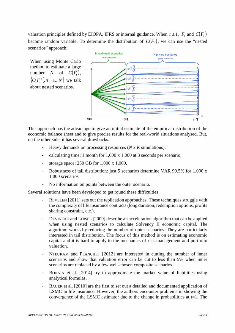
valuation principles defined by EIOPA, IFRS or internal guidance. When 1t , tF and tFC

become random variable. To determine the distribution of tFC , we can use the “nested

scenarios” approach:

When using Monte Carlo

method to estimate a large

number N of tFC ,

NnFC n

t ...1, we talk

about nested scenarios.

This approach has the advantage to give an initial estimate of the empirical distribution of the

economic balance sheet and to give precise results for the real-world situations analysed. But,

on the other side, it has several drawbacks:

- Heavy demands on processing resources (N x K simulations):

- calculating time: 1 month for 1,000 x 1,000 at 3 seconds per scenario,

- storage space: 250 GB for 1,000 x 1,000,

- Robustness of tail distribution: just 5 scenarios determine VAR 99.5% for 1,000 x

1,000 scenarios

- No information on points between the outer scenario.

Several solutions have been developed to get round these difficulties:

- REVELEN [2011] sets out the replication approaches. These techniques struggle with

the complexity of life insurance contracts (long duration, redemption options, profits

sharing constraint, etc.),

- DEVINEAU and LOISEL [2009] describe an acceleration algorithm that can be applied

when using nested scenarios to calculate Solvency II economic capital. The

algorithm works by reducing the number of outer scenarios. They are particularly

interested in tail distribution. The focus of this method is on estimating economic

capital and it is hard to apply to the mechanics of risk management and portfolio

valuation.

- NTEUKAM and PLANCHET [2012] are interested in cutting the number of inner

scenarios and show that valuation error can be cut to less than 5% when inner

scenarios are replaced by a few well-chosen composite scenarios.

- BONNIN et al. [2014] try to approximate the market value of liabilities using

analytical formulas,

- BAUER et al. [2010] are the first to set out a detailed and documented application of

LSMC in life insurance. However, the authors encounter problems in showing the

convergence of the LSMC estimator due to the change in probabilities at t=1. The

N real world scenarios

(outer scenarios)

K pricing scenarios

(inner scenarios)

t=1t=0 t=T


authors also measure the impacts on a fictional portfolio and fail to address the

problems applying these techniques to a real-world portfolio (complexity of

liabilities and assets, processing time, storage space, calculation tools, etc.). Finally,

the mechanism for selecting the regression base is not explained in detail.

- Another approach that could overcome some of the problems with nested stochastics

is to interpolate the results of the nested scenarios: so-called curve fitting.

Of all these techniques, the LSMC approach is emerging as the standard for internal modelling

in the life insurance industry, for several reasons:

- it can estimate the value of economic capital,

- it can be used to manage risk (ORSA): risk hedging, calculation of risk appetite

indicators,

- it is used in ALM studies: to determine optimal allocation, project portfolios, etc.

Below, we present the application of LSMC for a portfolio of life insurance contracts.

3 DESCRIPTION OF THE LSMC METHOD

The core idea of the least squares Monte Carlo (LSMC) method is to mimic the behaviour of

the liabilities using a function that includes all targeted risk factors as inputs (economic and/or

non-economic variables).

The precise behaviour (or pricing) function of the liabilities is unknown. It is approximated by

an approach based on the Taylor series approximation. This technique approximates the

behaviour of the function by a linear combination of basis functions applied to the targeted risk

factors:

M

i

tiit FLFC1

- *M is the number of regressors,

- 1, ,

k

t t tF F F represents the vector for the risk factors at time t,

- *k , total number of targeted risk factors,

- 1 2, ,

ML L L L represents a series of functions (the “regression

basis”),

- i represents the impact of the term ti FL on the quantity tFC .

The idea2 beyond this approximation derives from the properties of conditional expectations in

Lp -spaces, which are specific Hilbert spaces with countable orthonormal basis3. More

precisely, because the conditional expectancy ,i

E Y Z i I minimize the Euclidian distance

between the random variable 2Y L , it can be computed as the orthogonal projection of Y on

the subspace generated by the random variables ,i

Z i I . Moreover, because, in the

applications considered here the factors iZ are risk factors affecting the balance sheet of the

2 For a theoretical justification, see YOSIDA [1980] for the functional analysis part and NEVEU [1964] for the

definition and properties of conditional expectation. 3 See BECK et al. [2005] or YOSIDA [1980] p. 90.


insurer, one can assume, without restriction, that the set I is countable. For this reason, we will

consider in the rest of this paper the particular case of conditional expectancy with respect to a

subspace generated by a countable set of random variables.

Because of this assumption,

t

T

tu

uQt FutDFCfEFCt

1

, , which is in 2L , can thus be

expressed as a linear combination of a countable set of orthogonal functions measurable in 2L

t

i

tiit FLFC

1

where iii ,

,,1 are real numbers and ,, 21 LLL an orthogonal basis4

in 2L . If we choose *M a strictly positive natural integer, we can write:

MFC

FLFLFC

tM

Mi

tii

M

i

tiit

11

with:

- t

Mt

MM

i

tiitM FLFLFC 1

,

-

1Mi

tii FLM ,

- M

M LLLL ,,, 21 ,

- RiMiiM

,,,1 .

We have 0M in 2L when M , we arrive at the approximation ttM FCFC .

The M coefficients are then estimated in two stages:

1. Using the Monte Carlo method we generate N realisations of the random variables5

1C , , ...n n

t tF F n N ,

2. we calculate N

M by least squares regression of Cn

tF in n

t

M FL

2

1

: argmin CM

NN

n M n tM t t M

n

F L F

4 For ki ,...,1 iL is defined by

tit

i

FLF

L

: k

5 The Cn

tF are realisations of the random variable t

T

tu

ut FutDFCfFz

1

, such that

tQt FzEFCt


The result of this optimisation programme is the OLS estimator:

1

, , ,C

t t tNM N N M N N M N N N N

M t t t tL F L F L F F

with the M rows and N columns matrix:

- NnMk

n

tk

N

t

M

t

MN

t

NM FLFLFLFL

11

1, ,..., is an M N matrix,

- 1C , ,

N N N

t t tF C F C F ,

The LSMC function can be written

1

,M

NLS N

iM t i t

i

NM

Mt

C F L F

L F

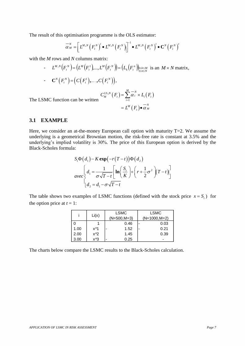
3.1 EXAMPLE

Here, we consider an at-the-money European call option with maturity T=2. We assume the

underlying is a geometrical Brownian motion, the risk-free rate is constant at 3.5% and the

underlying’s implied volatility is 30%. The price of this European option is derived by the

Black-Scholes formula:

1 2

2

1

2 1

1 1

2

exp

ln

t

t

S d K r T t d

Sd r T t

KT tavec

d d T t

The table shows two examples of LSMC functions (defined with the stock price tx S ) for

the option price at t = 1:

The charts below compare the LSMC results to the Black-Scholes calculation.

i Li(x)LSMC

(N=500,M=3)

LSMC

(N=1000,M=2)

0 1 0.46 0.03 -

1.00 x 1̂ 1.52 - 0.21 -

2.00 x 2̂ 1.45 0.39

3.00 x 3̂ 0.25 - -


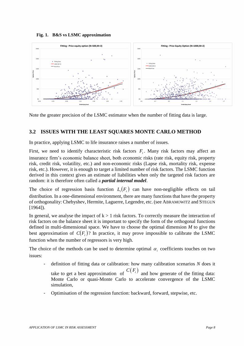
Fig. 1. B&S vs LSMC approximation

Note the greater precision of the LSMC estimator when the number of fitting data is large.

3.2 ISSUES WITH THE LEAST SQUARES MONTE CARLO METHOD

In practice, applying LSMC to life insurance raises a number of issues.

First, we need to identify characteristic risk factors tF . Many risk factors may affect an

insurance firm’s economic balance sheet, both economic risks (rate risk, equity risk, property

risk, credit risk, volatility, etc.) and non-economic risks (Lapse risk, mortality risk, expense

risk, etc.). However, it is enough to target a limited number of risk factors. The LSMC function

derived in this context gives an estimate of liabilities when only the targeted risk factors are

random: it is therefore often called a partial internal model.

The choice of regression basis function ti FL can have non-negligible effects on tail

distribution. In a one-dimensional environment, there are many functions that have the property

of orthogonality: Chebyshev, Hermite, Laguerre, Legendre, etc. (see ABRAMOWITZ and STEGUN

[1964]).

In general, we analyse the impact of k > 1 risk factors. To correctly measure the interaction of

risk factors on the balance sheet it is important to specify the form of the orthogonal functions

defined in multi-dimensional space. We have to choose the optimal dimension M to give the

best approximation of tFC ? In practice, it may prove impossible to calibrate the LSMC

function when the number of regressors is very high.

The choice of the methods can be used to determine optimal i coefficients touches on two

issues:

- definition of fitting data or calibration: how many calibration scenarios N does it

take to get a best approximation of t

C F and how generate of the fitting data:

Monte Carlo or quasi-Monte Carlo to accelerate convergence of the LSMC

simulation,

- Optimisation of the regression function: backward, forward, stepwise, etc.

Fitting : Price equity option (N=500,M=3)

0%

50%

100%

150%

200%

250%

0.50 0.70 0.90 1.10 1.30 1.50 1.70

Underlying Asset

Op

tio

n P

rice

Fitting Data

LSMC (M=3)

Real Price

Fitting : Price Equity Option (N=1000,M=2)

0%

50%

100%

150%

200%

250%

0.5 0.7 0.9 1.1 1.3 1.5 1.7

Underlying Asset

Op

tio

n P

rice

Fitting Data

LSMC (M=2)

Real Price


3.3 CONVERGENCE OF THE LSMC

3.3.1 CONVERGENCE OF THE LSMC UNDER THE RISK-NEUTRAL MEASURE tQ

We show that t

NLS

M FC , converges in 2L towards tFC under the risk-neutral measure tQ .

The convergence is demonstrated in two stages:

t

i

tiiLM

M

i

tiiLN

M

i

ti

N

it

NLS

M FCFLFLFLFC

111

,22

The first stage is based on the convergence of the Monte Carlo estimator. It can be simply

demonstrated using the law of large numbers and properties of orthogonal functions (see

appendix) and the second stage is obvious (see also Bauer et al [2010] section 5.3). As

mentioned in the very beginning of this section, this result is thru only because we assumed that

the set of risk factors is countable.

3.3.2 CONVERGENCE OF THE LSMC UNDER THE HISTORICAL MEASURE tP

In insurance, the distribution of risk factors tF is under the historical measure tP , implying that

the distribution of tFC is obtained under tP .

We therefore need to establish the convergence properties under the historical measure. BAUER

and al. [2010] specify that because of the change in measure at time t, the convergence of

t

NLS

M FC , toward tFC under the measure tP cannot be guaranteed.

Cft 2

Cft 2 Cft 1

Qt+1 Qt

t

T

tu

uQt FutDFCfEFCt

1

,

Cft 1

tF

Pt Qt+1

0 t t+1 t+2

tt FCF ,

0 t t+1 t+2

Change of

measure


In this section we will show that t

NLS

M FC , converges in probability toward tFC under the

measure tP . True, convergence in probability is weaker than 2L convergence, but it is still

stronger than convergence in distribution and enough to demonstrate the relevance of the LSMC

approach to valuing economic capital.

Property: t

NLS

M FC , converges in probability toward tFC under the historical measure tP

Proof:

In section 3.3.1, we showed that tLMN

t

NLS

M FCFC 2,,

under the measure tQ . This

implies that t

NLS

M FC , converges in probability toward tFC under the measure tQ .

lim 0 ,,

,t

N MLS NQM t t t N M

C F C F Q A

with ,

,;

LS N

N M M t tA C F C F and 0 .

The probability measures tQ and tP are equivalent 0 ,L2 ff , tt dQfdP , and f

a random variable with 1 tdQf :

tAMNt dQfAPMN ,

1 ,.

We have ffMNA

,1 , Lebesgue’s dominated convergence theorem6 implies that:

1

1

0

0

,

,

,lim lim

lim

N M

N M

t N M A t

A t

t

P A f dQ

f dQ

dQ

1 0,

limN MA

f because t

NLS

M FC , converges in probability toward tFC under the measure

tQ and the only possible values for 1,N MA

are 0 and 1. Thus t

NLS

M FC , converges in probability

toward tFC under the measure tP

3.4 CHOICE OF NUMBER OF SIMULATIONS AND NUMBER OF

REGRESSORS

i.e. *Met N : the LSMC function that approximates the value of component C of the

economic balance sheet at time t is:

tN

Mt

M

t

NLS

M FLFC ,

6 If the sequence nf converges pointwise to a function f and is dominated by some integrable function g in the

sense that nf g for all numbers n in the index set of the sequence, then f is integrable and the integral of n

f

converge towards f.


We showed in the previous section that t

NLS

M FC , converges toward tFC . Now, we are

interested in fixed *Met N , with an error between t

NLS

M FC , and tFC :

2

,, tt

NLS

M FCFCMN .

In absolute terms, this function does not have an optimum. Also, except in particular cases

(financial assets) we do not know tFC , so MN, is hard to quantify7. We can estimate it

by measuring the deviation between t

NLS

M FC , and the results of nested scenarios. But this

approach suffers from the major disadvantages of the nested scenarios approach (see section

2).

In practice, we measure the deviation between the t

NLS

M FC , function and a series of values for

tFC : we call these validation scenarios. The validation scenarios are chosen from the

distribution set of tFC . In general, some twenty points are enough to measure the quality of

the LSMC function.

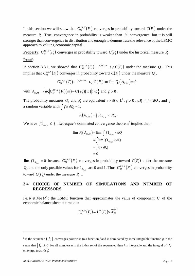
The chart below shows the estimation error (sum of square of deviations) for the price of a

European option from using the LSMC method:

Fig. 2. SSE on validation scenario

Note that the convergence is faster when N is very large:

- When N = 10,000, the sum of the square of pricing errors falls to 0.04% for

polynomial degree M = 3.

- When N = 2,000, the sum of the square of errors is always more than 0.13%

irrespective of the degree of the polynomial M.

7 The value 2

1

min CM

Nn M n t

t t M

n

F L F

is not an estimator of MN, as Cn

tF are realisations

of the random variable FutDFCfzT

tu

u

1

, and not values zEFCtQt

M=3

M=8

M=13

M=18

-

200

400

600

800

N=30kN=15k

N=8kN=2k

N=0.5k

SSE on validation scenarios

600 - 800

400 - 600

200 - 400

- - 200

bps


So, we fix a maximum acceptable error maxE , and try to determine maxmax

M , EEN such that

max

2,

Emax

max

tt

NLS

M FCFC E

E. To achieve this error we must fix N as high as possible:

- Depending on calculation and storage capacity: in general8 100,000 scenarios

provide good convergence of the LSMC result,

- We combine this with variance reduction techniques to achieve a better

convergence property.

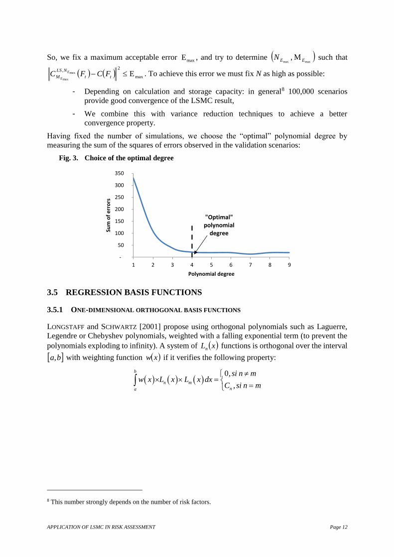
Having fixed the number of simulations, we choose the “optimal” polynomial degree by

measuring the sum of the squares of errors observed in the validation scenarios:

Fig. 3. Choice of the optimal degree

3.5 REGRESSION BASIS FUNCTIONS

3.5.1 ONE-DIMENSIONAL ORTHOGONAL BASIS FUNCTIONS

LONGSTAFF and SCHWARTZ [2001] propose using orthogonal polynomials such as Laguerre,

Legendre or Chebyshev polynomials, weighted with a falling exponential term (to prevent the

polynomials exploding to infinity). A system of xLn functions is orthogonal over the interval

ba, with weighting function xw if it verifies the following property:

0b

n m

na

, si n mw x L x L x dx

C , si n m

8 This number strongly depends on the number of risk factors.

-

50

100

150

200

250

300

350

1 2 3 4 5 6 7 8 9

Sum

of

err

ors

Polynomial degree

"Optimal"polynomial

degree


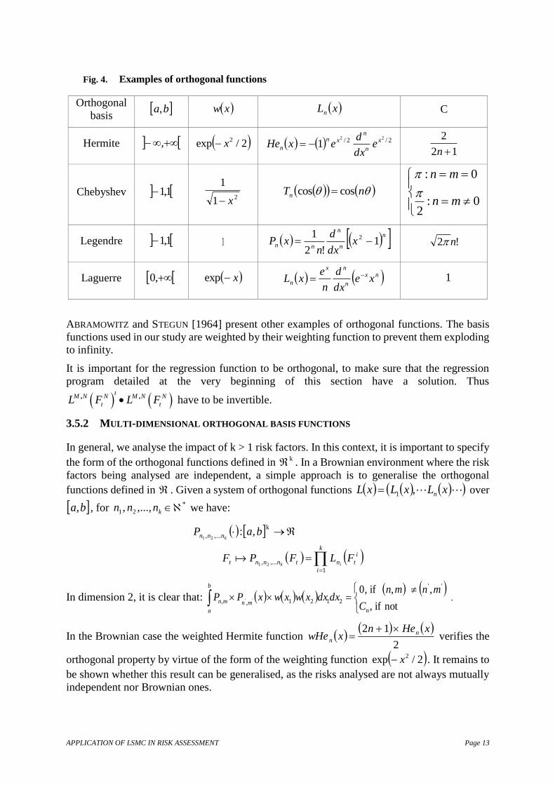
Fig. 4. Examples of orthogonal functions

Orthogonal

basis ba, xw xLn C

Hermite , 2/exp 2x 2/2/ 22

1 x

n

nxn

n edx

dexHe

12

2

n

Chebyshev 1,1 21

1

x nTn coscos

0:2

0:

mn

mn

Legendre 1,1 1 n

n

n

nn xdx

d

nxP 1

!2

1 2 !2 n

Laguerre ,0 xexp nx

n

nx

n xedx

d

n

exL 1

ABRAMOWITZ and STEGUN [1964] present other examples of orthogonal functions. The basis

functions used in our study are weighted by their weighting function to prevent them exploding

to infinity.

It is important for the regression function to be orthogonal, to make sure that the regression

program detailed at the very beginning of this section have a solution. Thus

, ,t

M N N M N N

t tL F L F have to be invertible.

3.5.2 MULTI-DIMENSIONAL ORTHOGONAL BASIS FUNCTIONS

In general, we analyse the impact of k > 1 risk factors. In this context, it is important to specify

the form of the orthogonal functions defined in k . In a Brownian environment where the risk

factors being analysed are independent, a simple approach is to generalise the orthogonal

functions defined in . Given a system of orthogonal functions xLxLxL n,1 over

ba, , for *

21 ,...,, knnn we have:

k

i

i

tntnnnt

nnn

FLFPF

baP

ik

k

1

,...,

k

,...,

21

21 , :

In dimension 2, it is clear that:

not if

,, if0 ''

2121,, ''

, C

mn mn , dxdxxwxwxPP

n

b

a

mnmn .

In the Brownian case the weighted Hermite function

2

12 xHenxwHe n

n

verifies the

orthogonal property by virtue of the form of the weighting function 2/exp 2x . It remains to

be shown whether this result can be generalised, as the risks analysed are not always mutually

independent nor Brownian ones.


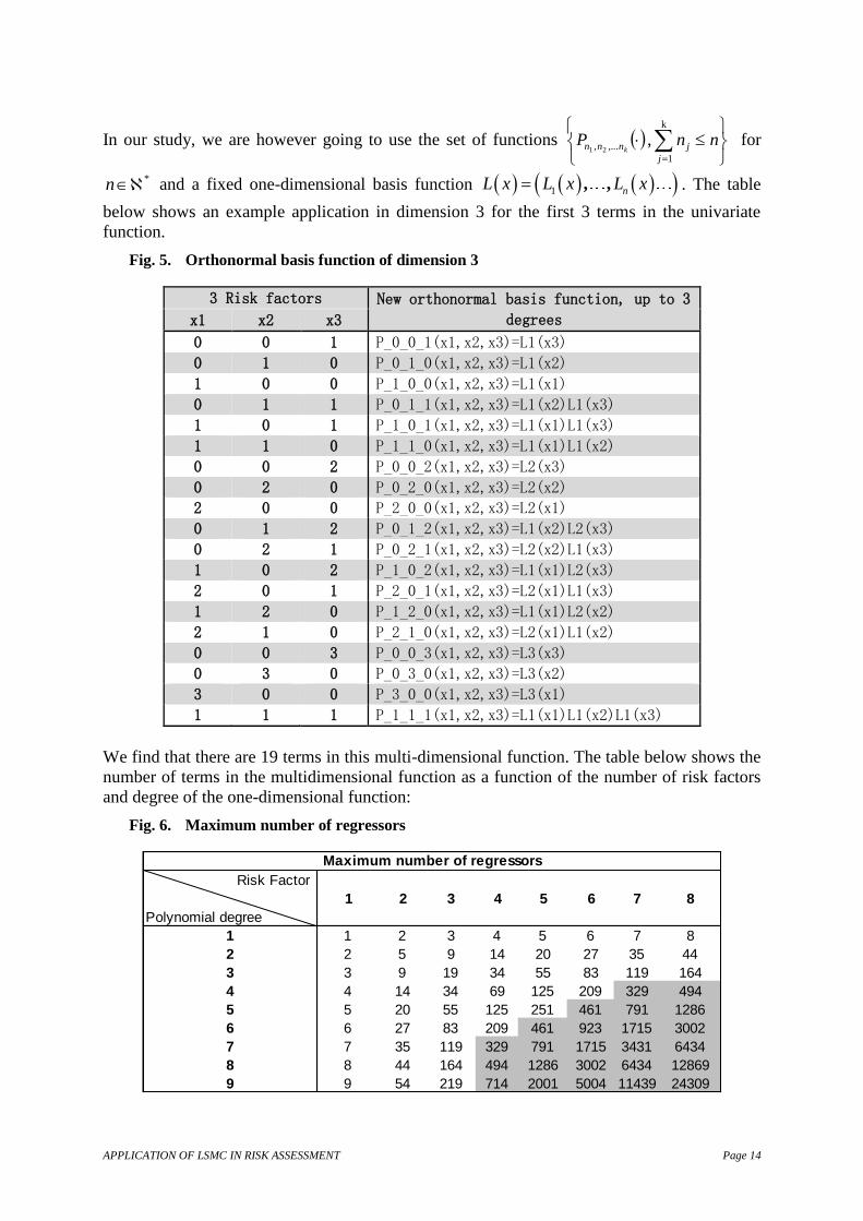
In our study, we are however going to use the set of functions , k

1

,..., 21

nnPj

jnnn k for

*n and a fixed one-dimensional basis function 1, ,

nL x L x L x . The table

below shows an example application in dimension 3 for the first 3 terms in the univariate

function.

Fig. 5. Orthonormal basis function of dimension 3

3 Risk factors New orthonormal basis function, up to 3

degrees x1 x2 x3

0 0 1 P_0_0_1(x1,x2,x3)=L1(x3)

0 1 0 P_0_1_0(x1,x2,x3)=L1(x2)

1 0 0 P_1_0_0(x1,x2,x3)=L1(x1)

0 1 1 P_0_1_1(x1,x2,x3)=L1(x2)L1(x3)

1 0 1 P_1_0_1(x1,x2,x3)=L1(x1)L1(x3)

1 1 0 P_1_1_0(x1,x2,x3)=L1(x1)L1(x2)

0 0 2 P_0_0_2(x1,x2,x3)=L2(x3)

0 2 0 P_0_2_0(x1,x2,x3)=L2(x2)

2 0 0 P_2_0_0(x1,x2,x3)=L2(x1)

0 1 2 P_0_1_2(x1,x2,x3)=L1(x2)L2(x3)

0 2 1 P_0_2_1(x1,x2,x3)=L2(x2)L1(x3)

1 0 2 P_1_0_2(x1,x2,x3)=L1(x1)L2(x3)

2 0 1 P_2_0_1(x1,x2,x3)=L2(x1)L1(x3)

1 2 0 P_1_2_0(x1,x2,x3)=L1(x1)L2(x2)

2 1 0 P_2_1_0(x1,x2,x3)=L2(x1)L1(x2)

0 0 3 P_0_0_3(x1,x2,x3)=L3(x3)

0 3 0 P_0_3_0(x1,x2,x3)=L3(x2)

3 0 0 P_3_0_0(x1,x2,x3)=L3(x1)

1 1 1 P_1_1_1(x1,x2,x3)=L1(x1)L1(x2)L1(x3)

We find that there are 19 terms in this multi-dimensional function. The table below shows the

number of terms in the multidimensional function as a function of the number of risk factors

and degree of the one-dimensional function:

Fig. 6. Maximum number of regressors

Risk Factor

Polynomial degree

1 2 3 4 5 6 7 8

1 1 2 3 4 5 6 7 8

2 2 5 9 14 20 27 35 44

3 3 9 19 34 55 83 119 164

4 4 14 34 69 125 209 329 494

5 5 20 55 125 251 461 791 1286

6 6 27 83 209 461 923 1715 3002

7 7 35 119 329 791 1715 3431 6434

8 8 44 164 494 1286 3002 6434 12869

9 9 54 219 714 2001 5004 11439 24309

Maximum number of regressors


3.6 REGRESSION MODEL

In the previous section, we saw that the number of terms of the LSMC functions could be very

high in the insurance context. There are various econometric techniques for selecting the best

model from a set of possible candidates. For instance (see HOCKING [1976]):

- Selection (forward): Start with a model containing only the constant, then add one

variable at each stage:

o at each stage, select the most significant variable,

o repeat until all the most significant variables have been selected.

- Elimination (backward): Start with a model containing all regressors and eliminate

one at each stage.

o at each stage, eliminate the least significant variable,

o repeat until all the least significant variables have been eliminated.

- bidirectional: a combination of forward/backward approaches (stepwise). Start

with a model containing only the constant.

o Carry out a forward selection, leaving open the possibility of dropping any of the

variables that becomes insignificant at each stage.

o Repeat until all the variables selected are significant and all the eliminated

variables are insignificant.

There are many criteria for significance ( 2R , AIC , BIC , pC , etc.). BAUER et al. [2010] show

that Mallow’s pC criterion works well in an LSMC context as it gives the best results in the

event of heteroskedasticity of residuals. The charts below show the number of regressors

obtained using the different configurations analysed:


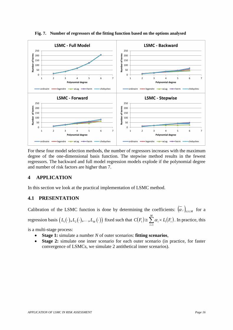
Fig. 7. Number of regressors of the fitting function based on the options analysed

For these four model selection methods, the number of regressors increases with the maximum

degree of the one-dimensional basis function. The stepwise method results in the fewest

regressors. The backward and full model regression models explode if the polynomial degree

and number of risk factors are higher than 7.

4 APPLICATION

In this section we look at the practical implementation of LSMC method.

4.1 PRESENTATION

Calibration of the LSMC function is done by determining the coefficients: Mii 1 for a

regression basis 1 2, , ,

ML L L fixed such that

M

i

tiit FLFC1

. In practice, this

is a multi-stage process:

Stage 1: simulate a number N of outer scenarios: fitting scenarios,

Stage 2: simulate one inner scenario for each outer scenario (in practice, for faster

convergence of LSMCs, we simulate 2 antithetical inner scenarios).

0

50

100

150

200

250

1 2 3 4 5 6 7

Nu

mb

er

of

term

s

Polynomial degree

LSMC - Full Model

ordinaire legendre wLag herm chebyshev

0

50

100

150

200

250

1 2 3 4 5 6 7

Nu

mb

er

of

term

s

Polynomial degree

LSMC - Backward


0

50

100

150

200

250

1 2 3 4 5 6 7

Nu

mb

er

of

tem

rs

Polynomial degree

LSMC - Forward


0

50

100

150

200

250

1 2 3 4 5 6 7

Nu

mb

er

of

term

s

Polynomial degree

LSMC - Stepwise



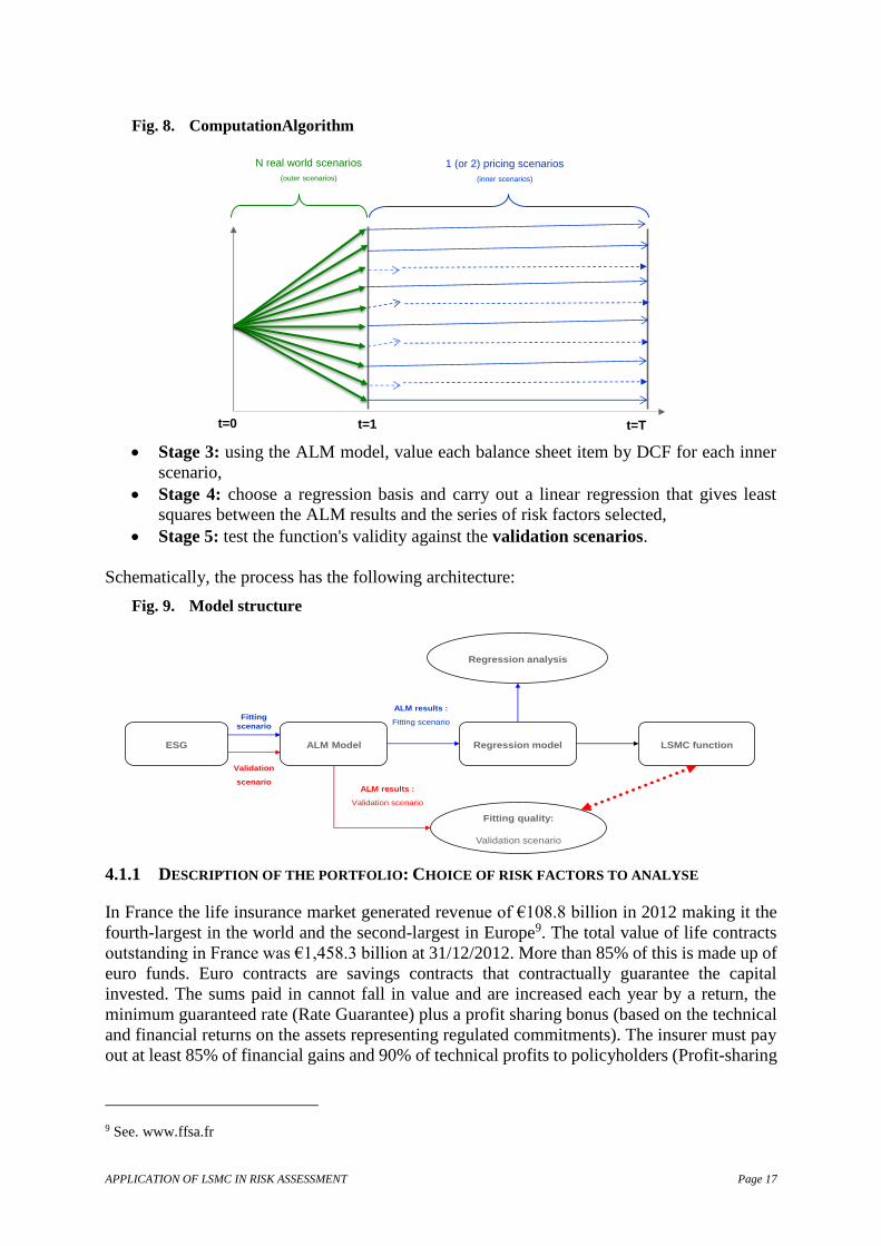
Fig. 8. ComputationAlgorithm

Stage 3: using the ALM model, value each balance sheet item by DCF for each inner

scenario,

Stage 4: choose a regression basis and carry out a linear regression that gives least

squares between the ALM results and the series of risk factors selected,

Stage 5: test the function's validity against the validation scenarios.

Schematically, the process has the following architecture:

Fig. 9. Model structure

4.1.1 DESCRIPTION OF THE PORTFOLIO: CHOICE OF RISK FACTORS TO ANALYSE

In France the life insurance market generated revenue of €108.8 billion in 2012 making it the

fourth-largest in the world and the second-largest in Europe9. The total value of life contracts

outstanding in France was €1,458.3 billion at 31/12/2012. More than 85% of this is made up of

euro funds. Euro contracts are savings contracts that contractually guarantee the capital

invested. The sums paid in cannot fall in value and are increased each year by a return, the

minimum guaranteed rate (Rate Guarantee) plus a profit sharing bonus (based on the technical

and financial returns on the assets representing regulated commitments). The insurer must pay

out at least 85% of financial gains and 90% of technical profits to policyholders (Profit-sharing

9 See. www.ffsa.fr

t=1t=0 t=T

N real world scenarios

(outer scenarios)

1 (or 2) pricing scenarios

(inner scenarios)

ESG ALM Model Regression model LSMC function

Regression analysis

Fitting quality:

Validation scenario

Fitting

scenario

Validation

scenarioALM results :

Validation scenario

ALM results :

Fitting scenario


option). In addition, income earned each year is definitively accrued. The insurer effectively

guarantees the accrued value of capital at all times (Surrender option).

To cover these regulated commitments, French life insurers are invested in the following asset

classes (Source: FFSA10): OECD sovereign debt: 32%, corporate bonds: 37%, equities,

property, investment funds and other assets: 25% and money markets: 6%. Euro contracts are

affected by market and technical risks. In this paper, we analyse the impact of the following

market risks:

- Rate risk, rise or fall,

- Risk of a fall in equities markets,

- Risk of a fall in the property market.

Note that it is simple to extend the technique presented here to non-economic risks

operationally.

4.1.2 ALM MODELLING

Results are based on the ALM model used by HSBC Assurances Vie. This software meets the

insurer’s aim of having a powerful stochastic modelling tool with easily auditable results. This

model is the reference tool used in all ALM work which allows us to value the economic balance

sheet and its various sensitivities. Besides stochastic simulations, it provides the following

functionalities:

- compliance with insurance rules by carrying out accounting closes,

- reproducing the insurer’s targets (including payments to policyholders),

- the option of generating stresses that impede the insurers’ targets,

- the option of using stochastic scenarios to value options embedded in the contracts.

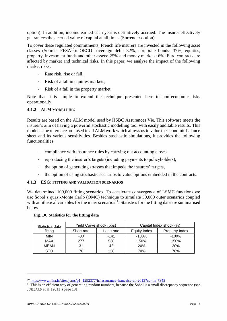
4.1.3 ESG: FITTING AND VALIDATION SCENARIOS

We determined 100,000 fitting scenarios. To accelerate convergence of LSMC functions we

use Sobol’s quasi-Monte Carlo (QMC) technique to simulate 50,000 outer scenarios coupled

with antithetical variables for the inner scenarios11. Statistics for the fitting data are summarised

below:

Fig. 10. Statistics for the fitting data

Statistics data fitting

Yield Curve shock (bps) Capital Index shock (%)

Short rate Long rate Equity Index Property Index

MIN -30 -141 -100% -100%

MAX 277 538 150% 150%

MEAN 31 42 20% 30%

STD 70 128 70% 70%

10 https://www.ffsa.fr/sites/jcms/p1_1292377/fr/lassurance-francaise-en-2013?cc=fn_7345 11 This is an efficient way of generating random numbers, because the Sobol is a small discrepancy sequence (see

JUILLARD et al. [2011]) page 181.

https://www.ffsa.fr/sites/jcms/p1_1292377/fr/lassurance-francaise-en-2013?cc=fn_7345


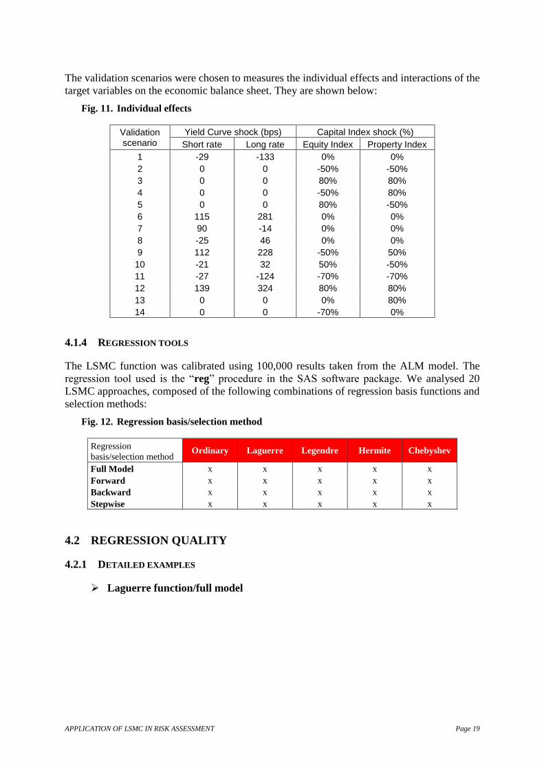
The validation scenarios were chosen to measures the individual effects and interactions of the

target variables on the economic balance sheet. They are shown below:

Fig. 11. Individual effects

Validation scenario

Yield Curve shock (bps) Capital Index shock (%)

Short rate Long rate Equity Index Property Index

1 -29 -133 0% 0%

2 0 0 -50% -50%

3 0 0 80% 80%

4 0 0 -50% 80%

5 0 0 80% -50%

6 115 281 0% 0%

7 90 -14 0% 0%

8 -25 46 0% 0%

9 112 228 -50% 50%

10 -21 32 50% -50%

11 -27 -124 -70% -70%

12 139 324 80% 80%

13 0 0 0% 80%

14 0 0 -70% 0%

4.1.4 REGRESSION TOOLS

The LSMC function was calibrated using 100,000 results taken from the ALM model. The

regression tool used is the “reg” procedure in the SAS software package. We analysed 20

LSMC approaches, composed of the following combinations of regression basis functions and

selection methods:

Fig. 12. Regression basis/selection method

Regression

basis/selection method Ordinary Laguerre Legendre Hermite Chebyshev

Full Model x x x x x

Forward x x x x x

Backward x x x x x

Stepwise x x x x x

4.2 REGRESSION QUALITY

4.2.1 DETAILED EXAMPLES

Laguerre function/full model


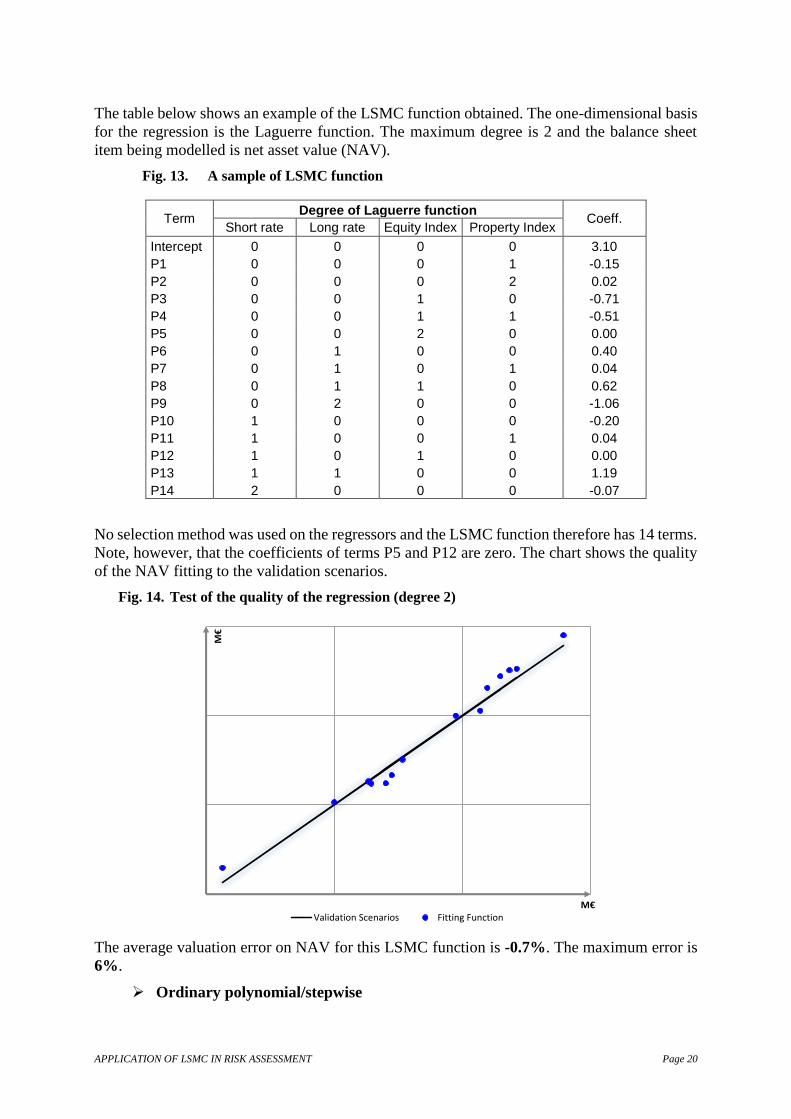
The table below shows an example of the LSMC function obtained. The one-dimensional basis

for the regression is the Laguerre function. The maximum degree is 2 and the balance sheet

item being modelled is net asset value (NAV).

Fig. 13. A sample of LSMC function

Term Degree of Laguerre function

Coeff. Short rate Long rate Equity Index Property Index

Intercept 0 0 0 0 3.10

P1 0 0 0 1 -0.15

P2 0 0 0 2 0.02

P3 0 0 1 0 -0.71

P4 0 0 1 1 -0.51

P5 0 0 2 0 0.00

P6 0 1 0 0 0.40

P7 0 1 0 1 0.04

P8 0 1 1 0 0.62

P9 0 2 0 0 -1.06

P10 1 0 0 0 -0.20

P11 1 0 0 1 0.04

P12 1 0 1 0 0.00

P13 1 1 0 0 1.19

P14 2 0 0 0 -0.07

No selection method was used on the regressors and the LSMC function therefore has 14 terms.

Note, however, that the coefficients of terms P5 and P12 are zero. The chart shows the quality

of the NAV fitting to the validation scenarios.

Fig. 14. Test of the quality of the regression (degree 2)

The average valuation error on NAV for this LSMC function is -0.7%. The maximum error is

6%.

Ordinary polynomial/stepwise

130

180

230

280

130 180 230 280

M€

M€Validation Scenarios Fitting Function


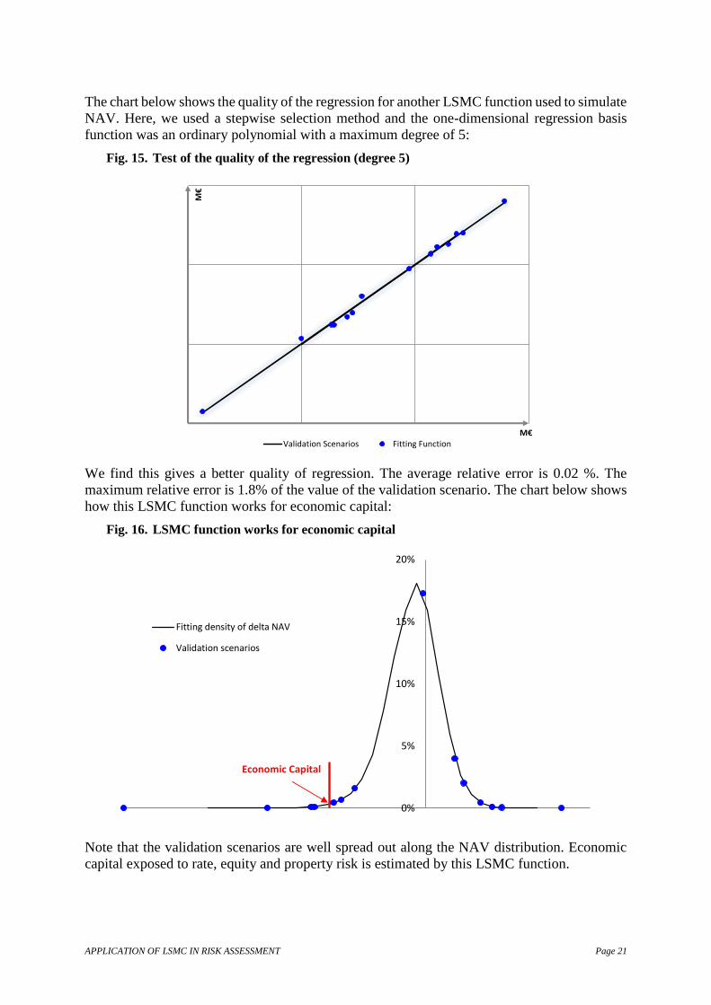
The chart below shows the quality of the regression for another LSMC function used to simulate

NAV. Here, we used a stepwise selection method and the one-dimensional regression basis

function was an ordinary polynomial with a maximum degree of 5:

Fig. 15. Test of the quality of the regression (degree 5)

We find this gives a better quality of regression. The average relative error is 0.02 %. The

maximum relative error is 1.8% of the value of the validation scenario. The chart below shows

how this LSMC function works for economic capital:

Fig. 16. LSMC function works for economic capital

Note that the validation scenarios are well spread out along the NAV distribution. Economic

capital exposed to rate, equity and property risk is estimated by this LSMC function.

130

180

230

280

130 180 230 280

M€

M€Validation Scenarios Fitting Function

Economic Capital

0%

5%

10%

15%

20%

-92 -72 -52 -32 -12 8 28 48

Fitting density of delta NAV

Validation scenarios


4.2.2 STATISTICS FOR THE TEST CASES

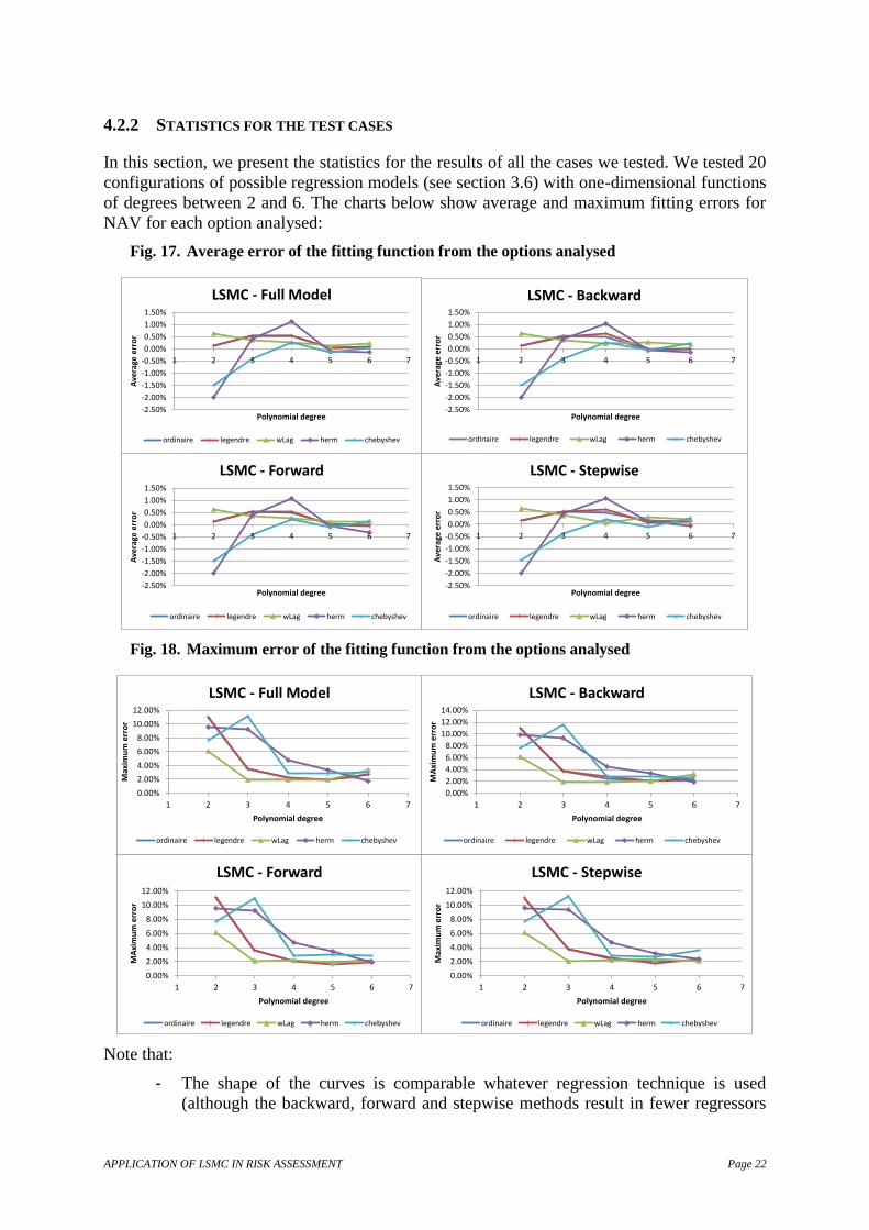
In this section, we present the statistics for the results of all the cases we tested. We tested 20

configurations of possible regression models (see section 3.6) with one-dimensional functions

of degrees between 2 and 6. The charts below show average and maximum fitting errors for

NAV for each option analysed:

Fig. 17. Average error of the fitting function from the options analysed

Fig. 18. Maximum error of the fitting function from the options analysed

Note that:

- The shape of the curves is comparable whatever regression technique is used

(although the backward, forward and stepwise methods result in fewer regressors

-2.50%

-2.00%

-1.50%

-1.00%

-0.50%

0.00%

0.50%

1.00%

1.50%

1 2 3 4 5 6 7

Ave

rage

err

or

Polynomial degree

LSMC - Full Model


-2.50%

-2.00%

-1.50%

-1.00%

-0.50%

0.00%

0.50%

1.00%

1.50%

1 2 3 4 5 6 7

Ave

rage

err

or

Polynomial degree

LSMC - Backward


-2.50%

-2.00%

-1.50%

-1.00%

-0.50%

0.00%

0.50%

1.00%

1.50%

1 2 3 4 5 6 7

Ave

rage

err

or

Polynomial degree

LSMC - Forward


-2.50%

-2.00%

-1.50%

-1.00%

-0.50%

0.00%

0.50%

1.00%

1.50%

1 2 3 4 5 6 7

Ave

rage

err

or

Polynomial degree

LSMC - Stepwise


0.00%

2.00%

4.00%

6.00%

8.00%

10.00%

12.00%

1 2 3 4 5 6 7

Max

imu

m e

rro

r

Polynomial degree

LSMC - Full Model


0.00%

2.00%

4.00%

6.00%

8.00%

10.00%

12.00%

14.00%

1 2 3 4 5 6 7

MA

xim

um

err

or

Polynomial degree

LSMC - Backward


0.00%

2.00%

4.00%

6.00%

8.00%

10.00%

12.00%

1 2 3 4 5 6 7

MA

xim

um

err

or

Polynomial degree

LSMC - Forward


0.00%

2.00%

4.00%

6.00%

8.00%

10.00%

12.00%

1 2 3 4 5 6 7

Max

imu

m e

rro

r

Polynomial degree

LSMC - Stepwise



than the full model, see section 3.6): valuation error falls with the degree of the

polynomial. However, implementing LSMC technique in practice becomes

impossible with a polynomial degree of more than 12.

- Note a substantial error margin (maximum error of over 2% when the basis

polynomial function has degree less than 3, in all cases). Valuation error starts to

stabilise at 4. The choice of optimum degree must therefore be either 4 or 5,

- The ordinary and Legendre polynomial both give very similar results because of the

constant weighting function (see appendix). The Laguerre polynomial stabilises

more quickly. The Hermite and Chebyshev polynomials are the least stable.

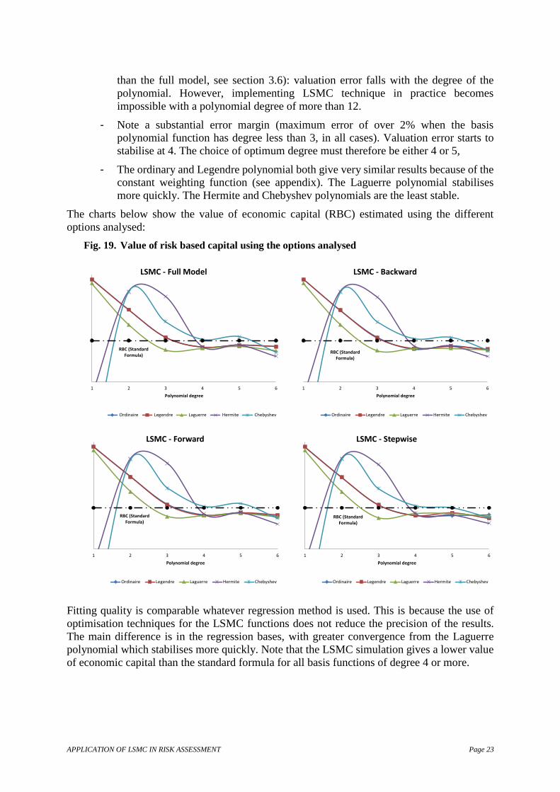
The charts below show the value of economic capital (RBC) estimated using the different

options analysed:

Fig. 19. Value of risk based capital using the options analysed

Fitting quality is comparable whatever regression method is used. This is because the use of

optimisation techniques for the LSMC functions does not reduce the precision of the results.

The main difference is in the regression bases, with greater convergence from the Laguerre

polynomial which stabilises more quickly. Note that the LSMC simulation gives a lower value

of economic capital than the standard formula for all basis functions of degree 4 or more.

RBC (Standard Formula)

20

25

30

35

40

45

1 2 3 4 5 6

M€

Polynomial degree

LSMC - Full Model

Ordinaire Legendre Laguerre Hermite Chebyshev


20

25

30

35

40

45

1 2 3 4 5 6

M€

Polynomial degree

LSMC - Backward



20

25

30

35

40

45

1 2 3 4 5 6

M€

Polynomial degree

LSMC - Forward



20

25

30

35

40

45

1 2 3 4 5 6

M€

Polynomial degree

LSMC - Stepwise



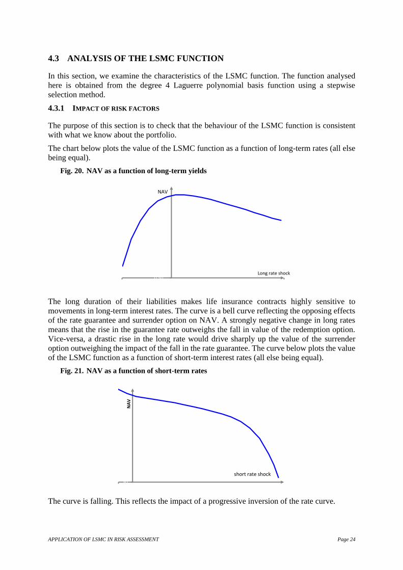
4.3 ANALYSIS OF THE LSMC FUNCTION

In this section, we examine the characteristics of the LSMC function. The function analysed

here is obtained from the degree 4 Laguerre polynomial basis function using a stepwise

selection method.

4.3.1 IMPACT OF RISK FACTORS

The purpose of this section is to check that the behaviour of the LSMC function is consistent

with what we know about the portfolio.

The chart below plots the value of the LSMC function as a function of long-term rates (all else

being equal).

Fig. 20. NAV as a function of long-term yields

The long duration of their liabilities makes life insurance contracts highly sensitive to

movements in long-term interest rates. The curve is a bell curve reflecting the opposing effects

of the rate guarantee and surrender option on NAV. A strongly negative change in long rates

means that the rise in the guarantee rate outweighs the fall in value of the redemption option.

Vice-versa, a drastic rise in the long rate would drive sharply up the value of the surrender

option outweighing the impact of the fall in the rate guarantee. The curve below plots the value

of the LSMC function as a function of short-term interest rates (all else being equal).

Fig. 21. NAV as a function of short-term rates

The curve is falling. This reflects the impact of a progressive inversion of the rate curve.

0.50

-140 320

Long rate shock

NAV

30

-30

NA

V

short rate shock


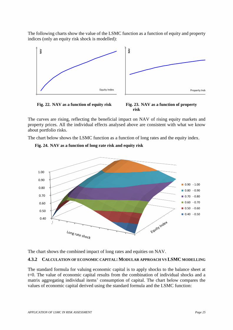
The following charts show the value of the LSMC function as a function of equity and property

indices (only an equity risk shock is modelled):

Fig. 22. NAV as a function of equity risk

Fig. 23. NAV as a function of property

risk

The curves are rising, reflecting the beneficial impact on NAV of rising equity markets and

property prices. All the individual effects analysed above are consistent with what we know

about portfolio risks.

The chart below shows the LSMC function as a function of long rates and the equity index.

Fig. 24. NAV as a function of long rate risk and equity risk

The chart shows the combined impact of long rates and equities on NAV.

4.3.2 CALCULATION OF ECONOMIC CAPITAL: MODULAR APPROACH VS LSMC MODELLING

The standard formula for valuing economic capital is to apply shocks to the balance sheet at

t=0. The value of economic capital results from the combination of individual shocks and a

matrix aggregating individual items’ consumption of capital. The chart below compares the

values of economic capital derived using the standard formula and the LSMC function:

170

0 2

NA

V

Equity Index

170

270

0 2

NA

V

Property Index

0.1

0.5

0.9

1.1

1.5

1.9 0.40

0.50

0.60

0.70

0.80

0.90

1.00

-…

0.90 - 1.00

0.80 - 0.90

0.70 - 0.80

0.60 - 0.70

0.50 - 0.60

0.40 - 0.50


Fig. 25. Economic capital: LSMC vs modular approach

Although the impact of stresses on the standard formula is lower, the value of economic capital

derived is still comparable to that from the LSMC model, mainly due to greater diversification

in the LSMC approach.

5 CONCLUSION

In this paper, we are interested in how least squares Monte Carlo technique (LSMC) can be

used in the field of life insurance. The levels of convergence under the historical measure

suggests that LSMC is effective in valuing economic capital. Results obtained show a good

quality fit (average error in NAV of less than 0.02% and maximum error of 1.8%). Also, the

LSMC function accurately reflects the behaviour of the liability being analysed.

Regarding the choice of regression technique, we saw that that stepwise selection method led

to the simplest LSMC function without impairing the precision of the results. When the number

of risk factors is higher than 7 and the degree of the basis polynomial function is higher than 7

only forward and stepwise selection give good results.

Regarding the basis functions analysed, we found that all functions examined gave good results.

Laguerre functions stabilised fastest. However, for practical implementation of LSMC

technique, the use of aggregation techniques (clustering, etc.) is essential due to the massive

calculation times required.

Also, it is hard to interpret the parameters of the LSMC function. In some cases, where the

number of terms in the function is very high, the LSMC function becomes unreadable. The

number of risk factors that can be analysed thus quickly reaches a limit.

Also, although the empirical results are relevant, further work is needed on the multi-

dimensional analysis of the orthogonality property of the functions analysed in this study.

Finally, in life insurance, it is essential to incorporate non-economic risk factors but here the

convergence properties remain unproven, mainly because of the change in probability. The

stability of the function over time makes it tempting to introduce initial wealth as a parameter

-47

-27

-7

13

33

53

73

93

Rates Equity + Vol Equity Property DiversificationEffect

Economic Capital

M€

LSMC Model Modular Approach (Similar to SII Approach)


as this reflects a capacity to absorb liability shocks. Calibration of the LSMC function over

multiple periods should be the next step.

6 APPENDICES

Convergence t

Q of the LSMC estimator

Let *M , we saw (see section 3) that we could approximate tFC by:

1

.M

M t

t M t i i t t M

i

C F C F L F L F

Assuming that k

tttt FFFF ,,, 21 is a Markov process vector.

Property: 1

t

M

M M Q t tA E L F C F

where MlklkM AA

,1, et tltkQlk FLFLEAt

,

Proof: for Mk ,...,1 , using the property of orthogonality12 of ,, 21 LLL we can

clearly show that 0, tMttk FCFCFL

* 0

0

0

0,

1

1

titk

M

i

ittkQ

M

i

tiittkQ

tMttkQ

tMttk

FLFLEFCFLE

FLFCFLE

FCFCFLE

FCFCFL

t

t

t

* In matrix form, this is rewritten:

1 1

1

1

1

for k 1,

for k,

for k M,

...

...

t t

t t

t t

t

M

i Q t i t Q t t

i

M

i Q k t i t Q k t t

i

M

i Q M t i t Q M t t

i

M

M M Q t t

E L F L F E L F C F

E L F L F E L F C F

E L F L F E L F C F

A E L F C F

12

ik si 0

ik si 0 titkQ FLFLE

t


Because of the orthogonality property of ,, 21 LLL , the matrix MA is a diagonal

matrix and all the elements on the diagonal must be greater than 0. It is therefore invertible.

The LSMC estimator is written as tN

Mt

M

t

NLS

M FLFC , where N

M is the OLS estimator:

1

, , ,C

t tNM N N M N N M N N N N

M t t t tL F L F L F F

with:

- NnMk

n

tk

N

t

M

t

MN

t

NM FLFLFLFL

11

1, ,..., ,

- 1C ,...,

N N N

t t tF C F C F ,

Property: ps. ,

tM

N

t

NLS

M FCFC

Proof: We need only show that ps. M

NN

M

Let , ,t

N M N N M N N

M t tA L F L F , then:

1

1

,

,

C

C

t tNN M N N N N

M M t t

t tM N N N NN

t tM

A L F F

L F FA

N N

We have 13 Mlk

N

n

n

tl

n

tk

N

M FLFLNN

A

,11

1

Applying the law of large numbers;

ps. 1

1

tltkQ

NN

n

n

tl

n

tk FLFLEFLFLN t

a.s.N

NMM

AA

N

In addition,

1 1

1,

C

tM N N N N

Nt t n n

k t t

n k M

L F C FL F F

N N

Applying the law of large numbers 1

1 ps.C

t

NNn n

k t t Q k t t

n

L F F E L F C FN

We have

1

1 a.s.

,C

t

t tM N N N NN

N t t N MMM M Q t t

L F FAA E L F C F

N N

a.s.N

NM M

13 Without impairing the general proof, we need only show that this is true for the cases N=2 and M=2.


7 REFERENCES

ABRAMOWITZ M., STEGUN I.A. [1964]: « Handbook of mathematical functions with formulas,

Graphs And mathematical Tables », National Bureau of standard, Applied Mathematic Series

55. June 1964.

BAUER D., BERGAMNN D.; REUSS A. [2010]: « Solvency II and Nested Simulations – a Least-

Squares Monte Carlo Approach » Proceedings of the 2010 ICA congress.

BECK V., MALICK J., PEYRÉ G. [2005] Objectif agrégation. Paris : H & K.

BONNIN F., JUILLARD M., PLANCHET F. [2014] « Best Estimate Calculations of Savings

Contracts by Closed Formulas - Application to the ORSA », European Actuarial Journal,

http://dx.doi.org/10.1007/s13385-014-0086-z.

BOYLE P. [1977] « Option: A monte carlo approach » Journal of Financial Economics 4, 323-

338

DEVINEAU L. ; LOISEL S. [2009]: « Construction d’un algorithme d’accélération de la méthode

des «simulations dans la simulation » pour le calcul du capital économique Solvabilité II »

Bulletin Français d'Actuariat 10, 17 (2009) 188-221

HOCKING, R. R. [1976] « The Analysis and Selection of Variables in Linear Regression »

Biometrics, 32, 1-49

IFERGAN E. [2013] « Mise en œuvre d’un calcul de best estimate », Actuarial Thesis, Université

Paris-Dauphine.

JUILLARD M., PLANCHET F., THÉROND P.E. [2011] Modèles financiers en assurance. Analyses

de risques dynamiques - seconde édition revue et augmentée, Paris : Economica (première

édition : 2005).

LONGSTAFF F.A.; SCHWARTZ E.S. [2001]: « Valuing American Options by Simulation: A

Simple Least-Squares Approach » The review of financial Studies, Spring 2001 Vol. 14, No. 1

pp. 113-147

NEVEU J. [1964] Bases mathématiques du calcul des probabilités, Paris: Masson.

NTEUKAM O.; PLANCHET F. [2012] « Stochastic evaluation of life insurance contracts: Model

point on asset trajectories & measurement of the error related to aggregation. » Insurance:

Mathematics and Economics, / Volume (Year): 51 (2012) Issue (Month): 3, Pages: 624-631

REVELEN J. [2011] « Replicating Portfolio et capital économique en assurance vie », Actuarial

Thesis, ISFA 04/01/2011.

WÜTHRICH M. V, BÜHLMANN H., FURRER H.[2008] Market-Consistent Actuarial Valuation,

Springer, ISBN: 978-3-540-73642-4

YOSIDA K. [1980] Functional Analysis, Berlin : Springer

http://people.math.sfu.ca/~cbm/aands/abramowitz_and_stegun.pdf

http://people.math.sfu.ca/~cbm/aands/abramowitz_and_stegun.pdf

http://www.ressources-actuarielles.net/C1256CFC001E6549/0/3690458B48D11A78C12579AE00695536

http://www.ressources-actuarielles.net/C1256CFC001E6549/0/3690458B48D11A78C12579AE00695536

http://www.ressources-actuarielles.net/C1256CFC001E6549/0/79B37FAD045F3B57C12579CF00449A9C

http://www.ressources-actuarielles.net/C1256CFC001E6549/0/79B37FAD045F3B57C12579CF00449A9C

http://www.ressources-actuarielles.net/C1256CFC001E6549/0/3741C4B04FF70A29C125809300569439

http://www.ressources-actuarielles.net/C12572BA0022FCE5/0/95B00A501A8740D4C125787A00758CB8

http://www.ressources-actuarielles.net/C12572BA0022FCE5/0/95B00A501A8740D4C125787A00758CB8

http://www.ressources-actuarielles.net/C12574E200674F5B/0/21DADBD66B2E2363C1257C080050C808

http://www.ressources-actuarielles.net/C1256F13006585B2/0/BA4AB88FEAF4ED3CC1257744003106EC

http://www.ressources-actuarielles.net/C1256F13006585B2/0/BA4AB88FEAF4ED3CC1257744003106EC

http://www.ressources-actuarielles.net/C1256CFC001E6549/0/6CE0568C702117A5C125795F0073802F

http://www.ressources-actuarielles.net/C1256CFC001E6549/0/6CE0568C702117A5C125795F0073802F

http://www.ressources-actuarielles.net/C1256CFC001E6549/0/AB539DCEBCC4E77AC12576C6004AFA67

http://www.ressources-actuarielles.net/C1256CFC001E6549/0/AB539DCEBCC4E77AC12576C6004AFA67

http://www.ressources-actuarielles.net/C12574E200674F5B/0/79AFD5A6F7564729C125763100495857

Documents

Version 1.7 Oberlain Jiaen Frédéric Nteukam T. Ren · PDF fileArticle 45 of the Solvency II Directive sets the rules ... taking into account all the contractual obligations that