Version 1.1 User Manual - Graz University of Technology · 1.3 Features of the current version Different levels of modeling Different neuron models: leaky-integrate-and-fire neurons,

CSIM : A Neural C ircuit SIMulatorVersion 1.1

User Manual

c©2002 The IGI LSM Groupwww.lsm.tugraz.at

July 10, 2006

This document is part of CSIM Release 1.1

Copyright 2002 The IGI LSM group

CSIM is free software; you can redistribute it and/or modify it under the terms of the GNU General Public License aspublished by the Free Software Foundation; either version 2, or (at your option) any later version.

CSIM is distributed in the hope that it will be useful, but WITHOUT ANY WARRANTY; without even the impliedwarranty of MERCHANTABILITY or FITNESS FOR A PARTICULAR PURPOSE. See the GNU General PublicLicense for more details.

To get a copy of the GNU General Public License point your browser to http://www.gnu.org/copyleft/gpl.html.

The IGI LSM groupInstitute for Theoretical Computer ScienceGraz University of TechnologyInffeldgasse 16/b, A-8010 Graz, [email protected], www.lsm.tugraz.at

www.lsm.tugraz.at

http://www.gnu.org/copyleft/gpl.html


[email protected]

www.lsm.tugraz.at

Contents

1 Preliminaries 5

1.1 What is CSIM ? . . . . . . . . . . . . . . . . . . . . . . . . . . . . . . . . . . . 5

1.2 About this Manual . . . . . . . . . . . . . . . . . . . . . . . . . . . . . . . . . 5

1.3 Features of the current version . . . . . . . . . . . . . . . . . . . . . . . . . . 6

1.4 Getting and Installing CSIM . . . . . . . . . . . . . . . . . . . . . . . . . . . 6

1.5 Compiling CSIM from the sources . . . . . . . . . . . . . . . . . . . . . . . . . 7

2 A short Tutorial 9

2.1 Creating Objects . . . . . . . . . . . . . . . . . . . . . . . . . . . . . . . . . . 9

2.2 Object Handles . . . . . . . . . . . . . . . . . . . . . . . . . . . . . . . . . . . 9

2.3 Setting Fields or Parameters . . . . . . . . . . . . . . . . . . . . . . . . . . . 9

2.4 Making connections . . . . . . . . . . . . . . . . . . . . . . . . . . . . . . . . 10

2.5 Recording . . . . . . . . . . . . . . . . . . . . . . . . . . . . . . . . . . . . . . 11

2.6 Setting up the input . . . . . . . . . . . . . . . . . . . . . . . . . . . . . . . . 11

2.7 Running the simulation . . . . . . . . . . . . . . . . . . . . . . . . . . . . . . 11

2.8 Plotting the recorded traces . . . . . . . . . . . . . . . . . . . . . . . . . . . . 12

3 Input and Output 13

3.1 Input Signals . . . . . . . . . . . . . . . . . . . . . . . . . . . . . . . . . . . . 13

3.2 Output . . . . . . . . . . . . . . . . . . . . . . . . . . . . . . . . . . . . . . . 14

3.2.1 Getting results of the last simulation . . . . . . . . . . . . . . . . . . . 14

3.2.2 Getting the results of a multi-stimulus simulation . . . . . . . . . . . . 15

4 Additional Topics 15

4.1 How the network is simulated . . . . . . . . . . . . . . . . . . . . . . . . . . . 15

4.2 Global fields . . . . . . . . . . . . . . . . . . . . . . . . . . . . . . . . . . . . . 16

4.3 Event driven simulation . . . . . . . . . . . . . . . . . . . . . . . . . . . . . . 16

5 Adding your own C++ model classes to CSIM 16

5.1 Recipe . . . . . . . . . . . . . . . . . . . . . . . . . . . . . . . . . . . . . . . . 17

5.2 Details . . . . . . . . . . . . . . . . . . . . . . . . . . . . . . . . . . . . . . . . 17

5.3 Hints for adding user defined models . . . . . . . . . . . . . . . . . . . . . . . 17

5.4 Setting and getting field values of objects . . . . . . . . . . . . . . . . . . . . 18

5.5 Implementaion . . . . . . . . . . . . . . . . . . . . . . . . . . . . . . . . . . . 18

5.5.1 Registering classes and fields . . . . . . . . . . . . . . . . . . . . . . . 18

2

5.5.2 reggen . . . . . . . . . . . . . . . . . . . . . . . . . . . . . . . . . . . . 19

6 CSIM command reference 21

6.1 Setting up a network simulation . . . . . . . . . . . . . . . . . . . . . . . . . . 21

6.1.1 create . . . . . . . . . . . . . . . . . . . . . . . . . . . . . . . . . . . . 21

6.1.2 set . . . . . . . . . . . . . . . . . . . . . . . . . . . . . . . . . . . . . . 21

6.1.3 connect . . . . . . . . . . . . . . . . . . . . . . . . . . . . . . . . . . . 22

6.2 Running the network simulation . . . . . . . . . . . . . . . . . . . . . . . . . 22

6.2.1 reset . . . . . . . . . . . . . . . . . . . . . . . . . . . . . . . . . . . . . 22

6.2.2 simulate . . . . . . . . . . . . . . . . . . . . . . . . . . . . . . . . . . . 22

6.3 Saving, loading and deleting networks . . . . . . . . . . . . . . . . . . . . . . 23

6.3.1 export . . . . . . . . . . . . . . . . . . . . . . . . . . . . . . . . . . . . 23

6.3.2 import . . . . . . . . . . . . . . . . . . . . . . . . . . . . . . . . . . . . 23

6.3.3 destroy . . . . . . . . . . . . . . . . . . . . . . . . . . . . . . . . . . . 23

6.4 Displaying/Getting information . . . . . . . . . . . . . . . . . . . . . . . . . . 23

6.4.1 get . . . . . . . . . . . . . . . . . . . . . . . . . . . . . . . . . . . . . . 23

6.4.2 list . . . . . . . . . . . . . . . . . . . . . . . . . . . . . . . . . . . . . . 24

6.4.3 version . . . . . . . . . . . . . . . . . . . . . . . . . . . . . . . . . . . . 25

7 CSIM model classe reference 25

7.1 AChannel Hoffman97 . . . . . . . . . . . . . . . . . . . . . . . . . . . . . . . . 25

7.2 AChannel Korngreen02 . . . . . . . . . . . . . . . . . . . . . . . . . . . . . . 25

7.3 ActiveCaChannel . . . . . . . . . . . . . . . . . . . . . . . . . . . . . . . . . . 26

7.4 ActiveChannel . . . . . . . . . . . . . . . . . . . . . . . . . . . . . . . . . . . 26

7.5 AHP Channel . . . . . . . . . . . . . . . . . . . . . . . . . . . . . . . . . . . . 26

7.6 AlphaSpikeFilter . . . . . . . . . . . . . . . . . . . . . . . . . . . . . . . . . . 27

7.7 AnalogFeedbackNeuron . . . . . . . . . . . . . . . . . . . . . . . . . . . . . . 27

7.8 AnalogInputNeuron . . . . . . . . . . . . . . . . . . . . . . . . . . . . . . . . 27

7.9 AnalogTeacher . . . . . . . . . . . . . . . . . . . . . . . . . . . . . . . . . . . 28

7.10 ArmModel . . . . . . . . . . . . . . . . . . . . . . . . . . . . . . . . . . . . . . 28

7.11 bNACNeuron . . . . . . . . . . . . . . . . . . . . . . . . . . . . . . . . . . . . 29

7.12 bNACOUNeuron . . . . . . . . . . . . . . . . . . . . . . . . . . . . . . . . . . 29

7.13 CaChannel Yamada98 . . . . . . . . . . . . . . . . . . . . . . . . . . . . . . . 30

7.14 cACNeuron . . . . . . . . . . . . . . . . . . . . . . . . . . . . . . . . . . . . . 31

7.15 cACOUNeuron . . . . . . . . . . . . . . . . . . . . . . . . . . . . . . . . . . . 31

7.16 CaGate Yamada98 . . . . . . . . . . . . . . . . . . . . . . . . . . . . . . . . . 32

3

7.17 CALChannel Destexhe98 . . . . . . . . . . . . . . . . . . . . . . . . . . . . . 33

7.18 CbNeuronSt . . . . . . . . . . . . . . . . . . . . . . . . . . . . . . . . . . . . . 33

7.19 CbNeuron . . . . . . . . . . . . . . . . . . . . . . . . . . . . . . . . . . . . . . 35

7.20 CbStOuNeuron . . . . . . . . . . . . . . . . . . . . . . . . . . . . . . . . . . . 37

7.21 CountSpikeFilter . . . . . . . . . . . . . . . . . . . . . . . . . . . . . . . . . . 39

7.22 DiscretizationPreprocessor . . . . . . . . . . . . . . . . . . . . . . . . . . . . . 39

7.23 dNACNeuron . . . . . . . . . . . . . . . . . . . . . . . . . . . . . . . . . . . . 39

7.24 dNACOUNeuron . . . . . . . . . . . . . . . . . . . . . . . . . . . . . . . . . . 40

7.25 DynamicSpikingCbSynapse . . . . . . . . . . . . . . . . . . . . . . . . . . . . 41

7.26 DynamicSpikingSynapse . . . . . . . . . . . . . . . . . . . . . . . . . . . . . . 42

7.27 DynamicStdpSynapse . . . . . . . . . . . . . . . . . . . . . . . . . . . . . . . 42

7.28 ExpSpikeFilter . . . . . . . . . . . . . . . . . . . . . . . . . . . . . . . . . . . 43

7.29 ExtInputNeuron . . . . . . . . . . . . . . . . . . . . . . . . . . . . . . . . . . 44

7.30 ExtOutLifNeuron . . . . . . . . . . . . . . . . . . . . . . . . . . . . . . . . . . 44

7.31 ExtOutLinearNeuron . . . . . . . . . . . . . . . . . . . . . . . . . . . . . . . . 45

7.32 ExtOutSigmoidalNeuron . . . . . . . . . . . . . . . . . . . . . . . . . . . . . . 45

7.33 GaussianAnalogFilter . . . . . . . . . . . . . . . . . . . . . . . . . . . . . . . 45

7.34 GVD cT Gate . . . . . . . . . . . . . . . . . . . . . . . . . . . . . . . . . . . . 46

7.35 GVD Gate . . . . . . . . . . . . . . . . . . . . . . . . . . . . . . . . . . . . . 46

7.36 HChannel Stuart98 . . . . . . . . . . . . . . . . . . . . . . . . . . . . . . . . . 46

7.37 HH K Channel . . . . . . . . . . . . . . . . . . . . . . . . . . . . . . . . . . . 47

7.38 HH Na Channel . . . . . . . . . . . . . . . . . . . . . . . . . . . . . . . . . . . 47

7.39 HHNeuron . . . . . . . . . . . . . . . . . . . . . . . . . . . . . . . . . . . . . . 47

7.40 HVACAChannel Brown93 . . . . . . . . . . . . . . . . . . . . . . . . . . . . . 48

7.41 IfbNeuron . . . . . . . . . . . . . . . . . . . . . . . . . . . . . . . . . . . . . . 49

7.42 Izhi Neuron . . . . . . . . . . . . . . . . . . . . . . . . . . . . . . . . . . . . . 50

7.43 KCAChannel Mainen96 . . . . . . . . . . . . . . . . . . . . . . . . . . . . . . 51

7.44 KChannel Korngreen02 . . . . . . . . . . . . . . . . . . . . . . . . . . . . . . 51

7.45 LifBurstNeuron . . . . . . . . . . . . . . . . . . . . . . . . . . . . . . . . . . . 52

7.46 LifNeuron . . . . . . . . . . . . . . . . . . . . . . . . . . . . . . . . . . . . . . 53

7.47 linear classification . . . . . . . . . . . . . . . . . . . . . . . . . . . . . . . . . 53

7.48 LinearNeuron . . . . . . . . . . . . . . . . . . . . . . . . . . . . . . . . . . . . 54

7.49 LinearPreprocessor . . . . . . . . . . . . . . . . . . . . . . . . . . . . . . . . . 54

7.50 linear regression . . . . . . . . . . . . . . . . . . . . . . . . . . . . . . . . . . 54

7.51 MChannel Mainen96 . . . . . . . . . . . . . . . . . . . . . . . . . . . . . . . . 54

4

7.52 MChannel Wang98 . . . . . . . . . . . . . . . . . . . . . . . . . . . . . . . . . 55

7.53 Mean Std Preprocessor . . . . . . . . . . . . . . . . . . . . . . . . . . . . . . . 55

7.54 MexRecorder . . . . . . . . . . . . . . . . . . . . . . . . . . . . . . . . . . . . 55

7.55 NPChannel McCormick02 . . . . . . . . . . . . . . . . . . . . . . . . . . . . . 56

7.56 PCAPreprocessor . . . . . . . . . . . . . . . . . . . . . . . . . . . . . . . . . . 56

7.57 Readout . . . . . . . . . . . . . . . . . . . . . . . . . . . . . . . . . . . . . . . 56

7.58 Recorder . . . . . . . . . . . . . . . . . . . . . . . . . . . . . . . . . . . . . . . 57

7.59 SICChannel Maciokas02 . . . . . . . . . . . . . . . . . . . . . . . . . . . . . . 58

7.60 SigmoidalNeuron . . . . . . . . . . . . . . . . . . . . . . . . . . . . . . . . . . 58

7.61 SpikingInputNeuron . . . . . . . . . . . . . . . . . . . . . . . . . . . . . . . . 58

7.62 SpikingTeacher . . . . . . . . . . . . . . . . . . . . . . . . . . . . . . . . . . . 59

7.63 StaticAnalogCbSynapse . . . . . . . . . . . . . . . . . . . . . . . . . . . . . . 59

7.64 StaticAnalogSynapse . . . . . . . . . . . . . . . . . . . . . . . . . . . . . . . . 59

7.65 StaticSpikingCbSynapse . . . . . . . . . . . . . . . . . . . . . . . . . . . . . . 59

7.66 StaticSpikingSynapse . . . . . . . . . . . . . . . . . . . . . . . . . . . . . . . . 60

7.67 StaticStdpSynapse . . . . . . . . . . . . . . . . . . . . . . . . . . . . . . . . . 60

7.68 Traubs HH K Channel . . . . . . . . . . . . . . . . . . . . . . . . . . . . . . . 61

7.69 Traubs HH Na Channel . . . . . . . . . . . . . . . . . . . . . . . . . . . . . . 61

7.70 TraubsHHNeuron . . . . . . . . . . . . . . . . . . . . . . . . . . . . . . . . . . 61

7.71 TriangularAnalogFilter . . . . . . . . . . . . . . . . . . . . . . . . . . . . . . . 63

7.72 UserAnalogFilter . . . . . . . . . . . . . . . . . . . . . . . . . . . . . . . . . . 63

1 Preliminaries

1.1 What is CSIM ?

CSIM is a tool for simulating heterogeneous networks composed of different model neuronsand synapses. This simulator is written in C++ with an MEX interface to Matlab. It isintended to simulate networks containing up to 10.000 neurons and up to the order of a fewmillions of synapses (the actual size depends of course on the amount of RAM available onyour machine).

1.2 About this Manual

This manual is intended to describe how to use CSIM from the (Matlab) users point of view. Itdoes not try to explain (or give an introduction to) the type of models which can be simulatedwith CSIM. Regarding neural modeling we refer the reader to [Dayan and Abbott, 2001] and[Gerstner and Kistler, 2002]. Furthermore Matlab programming knowledge is assumed.

This manual is also available in HTML format.

5

http://www.mathworks.com

1.3 Features of the current version

Different levels of modeling Different neuron models: leaky-integrate-and-fire neurons,compartmental based neurons, sigmoidal neurons. Different synapse models: staticsynapses and a certain model of dynamic synapses are available for spiking as well asfor sigmoidal neurons. Spike time dependent synaptic plasticity is also implemented.

Easy to use Matlab interface Since CSIM is incorporated into Matlab it is not necessaryto learn any other script laguage to set up the simulation. This is all done with Matlabscripts. Furthermore the results of a simulation are directly returned as Matlab arraysand hence any plotting and analysis tools available in Matlab can easily be applied.

Object oriented design We adopted an object oriented design for CSIM which is similarto the approaches taken in GENESIS and NEURON. That is there are objects (e.g. aLifNeuron object implements the standard leaky-integrate-and-fire model) which areinterconnected by means of some signal channels. The creation of objects, the connec-tion of objects and the setting of parameters of the objects is controlled at the level ofMatlab scipts whereas the actual simulation is done in the fast C++ core.

Fast C++ core Since CSIM is implemented in C++ and is not as general as GENESIS orNEURON simulations are performed quite fast. We also implemented some ideas fromevent driven simulators like SpikeNet which result on an average speedup of 3 (assum-ing an average firing rate of the neurons of 20 Hz and short synaptic time constants)compared to a standard fixed time step simulation scheme.

Runs on Windows and Unix (Linux) CSIM is developed on Linux but also runs underWindows XP (we have no more experience with Windows 98 yet, but it should also runthere) and should in principle run on any platform for which Matlab is available.

External Interface There is an external interface which allows CSIM to communicate withexternal programs. In this way one can for example control the miniature robot Kheperawith CSIM . This feature is not available in the Windows version.

1.4 Getting and Installing CSIM

CSIM is distributed under the GNU General Public License and can be downloaded fromhttp://www.igi.tugraz.at/csim.

To install CSIM perform the following steps:

1. Donwload CSIM from www.igi.tugraz.at/csim

2. Unzip the file csim-VER.zip where VER stands for the version you have downloaded.

This will create a subdirectory lsm and lsm/csim

3. Start Matlab and change into the directory lsm

4. Run the Matlab script install.m.

5. Add the path lsm to the Matlab search path; e. g.

6

http://www.bbb.caltech.edu/GENESIS/genesis.html

http://www.neuron.yale.edu

http://www.cnl.salk.edu/~arno/spikenet/

http://www.k-team.com/robots/khepera/index.html


http://www.igi.tugraz.at/csim

www.igi.tugraz.at/csim

• addpath(’/home/jack/lsm’)} or

• addpath(’C:\Work\Neuroscience\lsm’).

6. Change into the directory lsm/csim/demos and play around with them.

7. Have fun using CSIM !

1.5 Compiling CSIM from the sources

The instruction in this section are relevant in two cases

a) You do not have Linux (x86 architecture) or Windows as an operating system.1

b) You are planning to add your own models written in C++ to CSIM; see section 5 formore information on this topic.

Currently we support compilation using (GNU) make for Linux/Unix (which most liklyalso works for Mac OS X) and nmake (Microsoft Visual C++) for Windows (testedonly with Windows XP). The corresponding Makefiles are lsm/csim/src/Makefile andlsm\csim\src\Makefile.win.

Step by step instructions

1. To compile CSIM from the sources you must first setup Matlab’s mex utility properly.This can be achieved by issuing the command mex -setup at the Matlab prompt. Formore information on compiling MEX-files see the MEX-files Guide.

2. Optional steps: If you are planning to add your own models written in C++ to CSIM andare not using Linux or Windows you have to build the reggen tool which comes with CSIM(lsm/develop/reggen) for your platform.2

(a) Go to lsm/develop/reggen

(b) Run

• configure; make; for Linux/Unix(/Mac OS)• make.bat msvc for Windows XP with MS Visual C++

(c) If this fails read lsm/develop/reggen/INSTALL and try to fix the build. In this case youwill notice that reggen is a modified version of the well known tool doxygen.

3. Edit the corresponding Makefile to meet your system configuration.

4. Goto csim/src and run

• make for Linux/Unix(/Mac OS)

• nmake -f Makefile.win for Windows (XP)1The compiled MEX-files (csim.mexglx and csim.dll) which already come with CSIM should run on any

Linux or Windows operationg system respectively.2For Linux and Windows the precompiled reggen tool is located in lsm/develop/reggen/bin.

7

http://www.mathworks.com/support/tech-notes/1600/1605.html

We do not know whether this instructions work on systems other than Windows XP withMS Visual C++ and Linux with gcc (3.4 or higher). The External Interfaces/API section ofthe Mathworks web site and the Tech-Note 1601 contain valuable information about compilerrequirements for compiling C++ MEX files.

8

http://www.mathworks.com/access/helpdesk/help/techdoc/matlab_external/matlab_external.shtml

http://www.mathworks.com/support/tech-notes/1600/1601.shtml

2 A short Tutorial

In this section we will introduce CSIM by means of a simple example. We will use CSIM tosimulate a model where a leaky-integrate-and-fire (Sec. 7.46) neuron (LIF neuron) is drivenby a Poisson spike train which is transmitted by a dynamic synapse (Sec. 7.26).

input spike train LIF neuron

dynamic synapse

output spike train

2.1 Creating Objects

Each element/entity of the simple model we will implement, will be simulated by a correspond-ing object in CSIM . The following table shows the correspondence between the elements ofthe model and the class of the object used to simulate the element

element of model class of CSIM objectinput spike train SpikingInputNeurondynamic synapse DynamicSpikingSynapseLIF neuron LifNeuron

Hence, for the simulation to run one must create objects (Sec. 6.1.1) of the given class:

>> i=csim(’create’,’SpikingInputNeuron’);>> s=csim(’create’,’DynamicSpikingSynapse’);>> n=csim(’create’,’LifNeuron’);

2.2 Object Handles

The values i, s, and n returned by these create commands (Sec. 6.1.1) are the indices orhandles to the created objects. The handles are the only means to further access or modifyexisting objects.

2.3 Setting Fields or Parameters

Each of the created objects has several fields which usually correspond to a parameter of themodel which is implemented by the class of the object. To display for example all fields ofthe LifNeuron (Sec. 7.46) object we can use the command

>> csim(’get’,n);

This will yield the following output

9

0 : LifNeuronCm = 3e-08 (F)Rm = 1e+06 (Ohm)

Vresting = -0.06 (V)Vreset = -0.06 (V)Vinit = -0.06 (V)

Trefract = 0.003 (sec)Inoise = 0 (A)

Iinject = 0 (A)Vthresh = -0.045 (V)

Vm : 0 (V)type = 0

nSpikes : 0nIncoming : 0nOutgoing : 0

Some of the fields are parameters of the model (Cm, Rm, ...) which can be modified (denotedby the ’=’) others are internal state variables (Vm in this case) which can not be changed(denoted by the ’:’) and yet other provide auxiliary information (nSpikes, nIncoming, ...).See the Class Reference (Sec. 7) for details about fields of a particular object.

Suppose we want to change the absolut refractory period of the LIF neuron n to be of length2 ms and add a noisy current of 50 nA. This can be done with the command

>> csim(’set’,n,’Trefract’,0.002,’Inoise’,50e-9);

For the dynamic synapse s we choose parameters such that it will show a depressing behaviour:

>> csim(’set’,s,’W’,10,’U’,0.1,’D’,1,’F’,0.05);>> csim(’set’,s,’u0’,0.1,’r0’,1);

2.4 Making connections

So far we have generated three independent objects and set their fields to the desired values.Now we have to connect the objects to implement our simple model. We have to connect theinput i to the synapse s and the synapse to the neuron n:

>> csim(’connect’,n,s); % synapse to neuron>> csim(’connect’,s,i); % input to synapse

Note the the connect command (Sec. 6.1.3) uses the convention that the signal destination isthe first argument. Alternatively one can use the three argument form of the command:

>> csim(’connect’,n,i,s); % input to neuron via synapse

10

2.5 Recording

The model is now fully implemented. In addition we want to record traces of some quantitiesof interest. Suppose we want record the membrane potential and the spikes of neuron n aswell as the postsynaptic respones (the field psr) of the synapse. To do so we have to createa Recorder object (Sec. 7.58) and tell this object which fields from which objects to record.The recorder is created with the command

>> r=csim(’create’,’Recorder’);

and the following commands tell the recorder r to record the field psr of synapse s as its firsttrace and the field Vm of neuron n as its second trace:

>> csim(’connect’,r,s,’psr’);>> csim(’connect’,r,n,’Vm’);

Using the special field spikes the same syntax will be used to record the spikes of neuron nas the third trace of recorder r.

>> csim(’connect’,r,n,’spikes’);

The following figure summarizes which objects we have created and how they are connected:

SpikingInputNeuron LifNeuronDynamicSpikingSynapse Recorder

spikes

Vmpsr

2.6 Setting up the input

Before we are ready to run the simulation we have to define the spike train which shouldbe emitted by the input neuron i. In CSIM time varying input signals (Sec. 3.1) (analog orspiking) – also called the stimulus – are not considered to be properties/attributes of someobjects but are always explicitly specified. In the case of our example we will define a spiketrain with randomly drawn spike times (for details see Section 3.1):

>> S.spiking = 1; % 1 ... spike times, 0 ... analog data>> S.dt = NaN; % resolution for analog data>> S.idx = i; % index/handle of receiving object>> S.data = sort(rand(1,10)); % 10 random spikes in the interval 0 to 1 sec

2.7 Running the simulation

Now we are ready to run the simulation. The command

11

>> Tsim=1;>> csim(’simulate’,Tsim,S);

simulates the simple model for 1 sec starting at time t = 03 with the stimulus S.

2.8 Plotting the recorded traces

The traces recorded by the recorder can be obtained by the command

>> t=csim(’get’,r,’traces’)

which yields the output

t =channel: [1x3 struct]

A closer look at e.g. the first channel reveals that t.channel is a struct array with a similarstructure as we have seen above for the input signal:

>> t.channel(1)

ans =

idx: 1fieldName: ’psr’

data: [1x2000 double]spiking: 0

dt: 5.0000e-04

The output indicates that t.channel(1).data holds the psr trace(t.channel(1).fieldName) with a resolution of 0.5 ms (t.channel(1).dt). See theRecorder class documentation (Sec. 7.58) for details abput the structure of the trace output.Similarly t.channel(2) holds the the Vm trace and t.channel(3) holds the output spiketimes. Hence the following command will plot the psr trace

>> plot(t.channel(1).dt:t.channel(1).dt:Tsim,t.channel(1).data);

and the command

>> stem(t.channel(3).data,ones(size(t.channel(3).data)));

will draw the output spike train.

Using another set of plot commands one can easily create the following figure which shows theinput, the postsynaptic response and the output of the neuron (the voltage and the spikes)

3In general the simulation will be continued at the time where the last simulate command (Sec. 6.2.2)stopped. However the first simulate command – as in the case of the example – starts at time t = 0. Simulationtime can be reset to time t = 0 with the reset command (Sec. 6.2.1) csim(’reset’);.

12

input spike train

0 0.1 0.2 0.3 0.4 0.5 0.6 0.7 0.8 0.9 10

2

4

6

8x 10

−7

psr

[A]

postsynaptic response

0 0.1 0.2 0.3 0.4 0.5 0.6 0.7 0.8 0.9 1−0.08

−0.06

−0.04

−0.02

0

Vm

[V]

time [sec]

membrane potential and spikes

The full code of this example is contained as the file first model.m in the demo directory ofthe CSIM package.

3 Input and Output

3.1 Input Signals

When runing a network simulation via csim(’simulate’,...); one can specify input signalslike in the command

>> csim(’simulate’,Tsim,S);

where S is a struct array with the following fields:

• S(i).idx : array of handles of objects which should receives this signal

• S(i).spiking : binary flag (0/1) which determines if S(i).data should be interpretedas spike times or as an analog signal

• S(i).dt : time discretization; for analog signals (S(i).spiking=0) only

• S(i).data : signal data: vector of the analog values (S(i).spiking=0) or spike times(S(i).spiking=1)

Note that csim(’simulate’,...); accepts an arbirary number of such struct arrays. Seedocumentation of the simulate command (Sec. 6.2.2).

13

http://www.lsm.tugraz.at/csim

3.2 Output

If one simulates a network then one also wants to record the quantities of interest. In ourintroductory example (Sec. 2) we were interested in the membrane potential of the leaky-integrate and fire neuron. CSIM can record any field of any object by means of Recorder(Sec. 7.58) objects. The following code fragment shows how to set up a Recorder to recordthe membrane potential (Vm) of a LifNeuron (Sec. 7.46) object with handle n.

>> rec = csim(’create’,’Recorder’);>> csim(’connect’,rec,n,’Vm’);

Note that one Recorder object can record an arbitrary number of fields from arbitrary objects.

3.2.1 Getting results of the last simulation

After a network simulation via a command like

>> csim(’simulate’,Tsim,InputSignal);

the recorded data of the the last simulation Recorder rec can be obtained by the command

>> R=csim(’get’,rec,’traces’);

The exact structure of R for the recorder rec depends on the value of the field commonChannelsof the Recorder (Sec. 7.58) object.

commonChannels = 0 In this case (default) R is a struct array with the only field channelwhich is in turn a struct array with a similar structure as an input signal (Sec. 3.1). That is

• R.channel(j).idx : handle of the object from which field the data was recorded

• R.channel(j).spiking : binary flag (0/1) which determines if data should be inter-preted as spike times or as an analog signal

• R.channel(j).dt : time discretization; for analog signals only

• R.channel(j).data : signal data : vector of the analog values or spike times. Notethat the data always starts at time t = 0.

• R.channel(j).fieldName : name of the recorded field

commonChannels = 1 In this case R has two fields:

• R.data : A double array where R.data(j,s) is the s-th recorded value of the j-th fieldrecorded. Note that the data always starts at time t = 0. Remark: The number of valueswhich are recorded depends on the field dt of the Recorder object (Sec. 7.58).

• R.info : A struct array where R.info(j).idx is the handle of the object from whichthe field R.info(j).fieldName is recorded.

14

3.2.2 Getting the results of a multi-stimulus simulation

Reminder: The command

>> R=csim(’get’,rec,’traces’);

returns only the results of the last simulation. In the case of a multi-stimulus simulation withstimulus array S of length n this command returns only the result of the simulation withstimulus S(n).

To get the results of all n simulations one has to use

>> R=csim(’simulate’,Tsim,S);

In that case R contains the results of all n stimulations. R{r}(s).channel contains therecorded data of the r-th recorder during the s-th simulation (1 ≤ s ≤ n). R{r}(s).channelis of the format as described in Section 3.2.1.

4 Additional Topics

4.1 How the network is simulated

CSIM employs a fixed time step simulation scheme for the integration of the differentialequations involved (represented by objects). Currently all objects use the exponential Eulermethod with the same integration time step (see Section 4.2).

During each time step a certain method (advance) is called for each object part of thesimulation. There is a fixed schedule which depends a) on the class of the object and b) onthe time of creation. Here is the order of the classes.

1. Neuron

2. Synapse

3. Recorder

This means that all objects of classes derived from a generic Neuron are advanced first followedby objects of classes derived from a generic Synapse and so on.

Note that for example a more detailed neuron model (like the CbNeuron (Sec. 7.19)) has toadvance all its child objects like ion channels.

After a csim(’simulate’,...) command returns the network is kept in its current stateat this time t. A further csim(’simulate’,...) command continues the simulation at thistime t. Use csim(’reset’); to reset the simulation to time t = 0.

Note that recorded traces you get by the appropriate get command (Sec. 6.4.1) always startat time t = 0.

15

4.2 Global fields

There are a few fields which determine the global (i.e. not object specific) behavior of CSIMwhich can be modified via the set command (Sec. 6.1.2):

>> csim(’set’,<fieldname>,<value>);

Read/writeable fields

dt The integration time step used by all objects

randSeed The seed value for the random number generator

verboseLevel How much stuff should be written to the console window (no effect yet!).

nThreads Number of threads to use for simulation (no effect yet!). The multi-threadedversion of CSIM is currently under development.

spikeOutput Flag: 1 ... always output spikes as last cell element, 0 do not output spikes(obsolete).

The following fields are read-only:

t The current virtual (simulation) time

step The current time step; i.e. step=t/dt;

4.3 Event driven simulation

Since in a typical simulation the firing rate of the neurons is about 30 Hz and the time constantof a synaptic current is typically about 3ms most of the time a synapse is “idle”. Thisobservation encouraged us to implement some ideas of event driven simulators like SpikeNet4:We decided to cut off the very far tail of the exponential decaying synaptic responses (after5 time constants) and remove those synapses from the list of active synapses (which areadvanced every time step). A synapse is re-activated if it receives a further spike. For largenetworks with lots of synapses these idea results in an average speed-up of 2 to 3.

5 Adding your own C++ model classes to CSIM

This section describes how a user can add its own models to CSIM at the C++ level.4http://www.cnl.salk.edu/~arno/spikenet/

16



5.1 Recipe

1. Create a copy of that existing model which is closest to that you wish to implement inthe directory lsm/csim/src. In the following we assume that the related files are calledMyModel.h and MyModel.cpp.

2. Implement your model.

3. Add you model to CSIM:

• Linux/Unix/: Add MyModel.o to the list of objects in the Makefile.

• Windows: Add MyModel.obj to the list of objects in the Makefile.win.

4. Compile CSIM:

• Linux/Unix/: Run the command make

• Windows: Run the command nmake -f Makefile.win

5. Use your model!

5.2 Details

During the compilation of CSIM a tool called reggen is used to generate wrapper code whichallows you to access the parameters of your model from the Matlab level. This frees you fromthe tedious work of writing lots of code for getting and setting such fields. For more detailsabout this issue see the subsection 5.4.

If you are not using Linux or Windows you have to build the reggen tool which comes withCSIM (lsm/develop/reggen) for your platform.5

1. Go to lsm/develop/reggen

2. Run

• configure; make; for Linux/Unix(/Mac OS)

• make.bat msvc for Windows XP with MS Visual C++

3. If this fails read lsm/develop/reggen/INSTALL and try to fix the build. In this caseyou will notice that reggen is a modified version of the well known tool doxygen.

5.3 Hints for adding user defined models

• Don’t forget the line DO_REGISTERING in the class declaration of you model.

• Use doxygen comments to document your model.5For Linux and Windows the precompiled reggen tool is located in lsm/develop/reggen/bin.

17

5.4 Setting and getting field values of objects

At the Matlab level CSIM allows you to set and get values of fields of objects by means ofthe commands

v=csim(’get’,o,fieldname)

csim(’set’,o,fieldname,value)

where o is the handle of the object returned by

o=csim(’create’,classname)

and fieldname is a string identifying the field (i.e. the name of the field).

5.5 Implementaion

We implemented this mechanism using four classes:

• csimClass : the base classes of all classes in CSIM which implements the basic set andget methodes for accessable fields

• csimClassInfoDB : a container (of csimClassInfo objects) where information about allthe (at the matlab level) available classes is stored

• csimClassInfo : which stores information (accessible fields, description) about a certainclass

• csimFieldInfo : stores information about a certain field of a given class

5.5.1 Registering classes and fields

To make the set and get methodes of a class derived from csimClass work one has to registerthis class via csimClassInfoDB::registerCsimClass() and then to register each member variablewhich we want to be an accessable field via csimClassInfo::registerField() .

Class member variable of the types

• double and double ∗

• float and float ∗

• int and int ∗

can be made accessible fields.

Each field has the following associated information (see csimFieldInfo )

18

• access : READWRITE or READONLY

• units

• lower and upper bound

• size : the number of elements if the field is of type float ∗, double ∗, or int ∗

5.5.2 reggen

It woul be a tedious work to code all the csimClassInfoDB::registerCsimClass() and csim-ClassInfo::registerField() function calls by hand. So we decided to generate it automaticallyfrom the source code. We use a tool named reggen (a quick and dirty hack based on doxygen)to gather the infomation from the source code and its doxygen style documentation. reggenwrites all relevant function calls to register fields an classes to registerclass.i

Default behaviour of \c reggen

• public class member variables are registered as READWRITE fields

• protected class member variables are registered as READONLY

• private class member variables are not registered.

• no units are assumed (i.e. a dimensionless field)

• lower and upper bound are set to -Inf and +Inf respectively

• an warning is issued if no size information is given for arrays

• the brief doxygen comment is used as descriptio of the field

• the brief doxygen comment of a class is used as its description

Specifying information for use by reggen If you want to register a class you just putthe macro DO REGISTERING somewhere in the class definition.

For each of the member variables where you want to change the default behaviour of reggenyou have to put a doxygen brief comment where you specify the relevant information.

Example 1 Make the float variable S a read-writable field with units Volt and a lower andupper bound of -1 and +1 respectively:

//! A voltage scale factor [readwrite; units=Volt; range=(-1,1);]

float S;

19

Example 2 Make the double variable ∗A a read-only field with 20 elements, units Ohm,and a lower and upper bound of -100 and +100 respectively:

//! A voltage scale factor [readonly; size=20; units=Ohm; range=(-100,100);]

double *A;

Source code of reggen

• Currently reggen is maintained in lsm/develop/reggen .

• The relevant source file is lsm/develop/reggen/src/defgen.cpp .

• The binaries are lsm/develop/reggen/bin/reggen for Linux andlsm/develop/reggen/bin/reggen.exe for windows.

• To compile reggen under Linux type

cd lsm/develop/reggen; ./configure; make

• To compile reggen under Windows XP with MS Visual C++ type

cd lsm/develop/reggen; make.bat msvc

20

6 CSIM command reference

The common form of all CSIM commands is

csim(command,...);

where command is one of the following strings:

• ’create’ (Sec. 6.1.1) : Create an object of a certain class• ’set’ (Sec. 6.1.2) : Set fields of an object• ’connect’ (Sec. 6.1.3) : Connect objects• ’get’ (Sec. 6.4.1) : Get field values of an object• ’reset’ (Sec. 6.2.1) : Reset the simulation to t = 0.0• ’simulate’ (Sec. 6.2.2) : Simulate the network• ’export’ (Sec. 6.3.1) : Export the network for saving it• ’import’ (Sec. 6.3.2) : Import a loaded network• ’destroy’ (Sec. 6.3.3) : Destroy/delete the current netork• ’list’ (Sec. 6.4.2) or ’ls’ (Sec. 6.4.2) List various items• ’version’ (Sec. 6.4.3) : Print out a version string

A detailed description of each of the commands follows.

6.1 Setting up a network simulation

6.1.1 create

• idx=csim(’create’,class); creates an object of the class specified by the string classand returns a uint32 index or handle for the created object. This index/handle is theonly means to access the created object.

• idx=csim(’create’,class,N); creates N objects of the class specified by the stringclass and returns a uint32 vector of indices/handles for the created objects.

The handles returned by idx=csim(’create’,...); are used to identify the objects later in’set’, ’get’ and ’connect’ calls.

See the Class Reference (Sec. 7) for a full description of all available classes.

6.1.2 set

• csim(’set’,field,value); sets the network field (Sec. 4.2) specified by the stringfield to value.

• csim(’set’,idx,field,value); sets the field specified by the string field of theobject with index/handle idx to value. idx can also be a vector of indices/handles ofobjects of the same class.

If idx is a vector and value is a scalar then the fields of all objects are set to value.

If idx and value are vectors of the same size then the field field of all objects idx(i)is set to value(i).

21

• csim(’set’,idx,f1,v1,f2,f2,...,fn,vn); sets the fields specified by the strings f1,f2, ..., fn of the object with index/handle idx to the values v1, v2, ... vn. idx and v1,v2, ... vn can also be vectors.

6.1.3 connect

• csim(’connect’,dstIdx,srcIdx); sets up a signal flow from the source srcIdx object(e.g. a synapse) to the destination object dstIdx (e.g. the postsynaptic neuron) wheredstIdx and srcIdx are indices/handles to objects.

dstIdx and srcIdx can also be vectors. In that case for each i=1:length(srcIdx); asignal flow dstIdx(i)← srcIdx(i) is set up.

• csim(’connect’, dstIdx, srIdx, viaIdx); for each i=1:length(srcIdx); a signalflow of the form dstIdx(i)← viaIdx(i)← srcIdx(i) is set up where dstIdx, srcIdx,and viaIdx are vectors of the same length of indices/handles to objects.

• csim(’connect’,recIdx,objIdx,fieldName); connects the object with handleobjIdx to the recorder with handle recIdx. The recorder recIdx will then recorda trace of the values of the field fieldName of the objects specified by the vector ofhadles objIdx.

6.2 Running the network simulation

6.2.1 reset

csim(’reset’); resets the simulation time t back to t = 0.0.

6.2.2 simulate

• csim(’simulate’,Tsim,InputSignals); runs the network simulation for Tsim sec-onds starting at the time where the last simulate command stopped with input signalsInputSignals (Sec. 3.1).

• csim(’simulate’,Tsim,I1,I2,...,In); same as above but with input signals I1 toIn. There is no special meaning in the ordering of the input signals. It is equvivalentto concatenate I1 to In into one struct array and pass this array as the single inputsignal.

• R=csim(’simulate’,Tsim,InputSignals);same as csim(’simulate’,Tsim,InputSignals); but in addition returns the cell arrayR which holds the output (traces) of all Recorder objects (Sec. 3.2).

• R=csim(’simulate’,Tsim,I1,I2,...,In);same as csim(’simulate’,Tsim,I1,I2,...,In); but in addition returns the cell arrayR which holds the output (traces) of all Recorder objects (Sec. 3.2).

22

• R=csim(’simulate’,Tsim,I1,I2,...,In);same as csim(’simulate’,Tsim,I1,I2,...,In); but in addition returns the cell arrayR which holds the output (traces) of all Recorder objects (Sec. 3.2).

6.3 Saving, loading and deleting networks

6.3.1 export

The command

net = csim(’export’);

produces a struct array net which contains all information about the current network simu-lation which is needed to set up the simulation. Using save file.mat net you can save thewhole network simulation.

NOTE: The struct array net returned by net=csim(’export’); is only intended to be savedto disk for later use by csim(’import’,net); and does not have a human readable form.

6.3.2 import

The command

csim(’import’,net);

allows you to set up a network simulation from the struct array net which has previously beengenerated by net = csim(’export’);. In combination with the matlab command load thisCSIM command serves the purpose of loading a simulation from disk.

If the current network (either explicitly specified or default network) does not contain anyobjects the net will be imported into that network. If there are already objects a new networkwill be created and and net will be imported to that.

NOTE: The struct array net returned by net=csim(’export’); does not contain informationabout the current state of the simulation at time t. Hence it is only possible to start simulationbased on such an arry at time t = 0.0.

6.3.3 destroy

csim(’destroy’); all the networks.

6.4 Displaying/Getting information

6.4.1 get

• csim(’get’); diplays the values of the global fields (Sec. 4.2)

• v=csim(’get’,field); return the value of the global field (Sec. 4.2) specified by thestring field

23

• csim(’get’,idx); displays the values of all fields of the object specified by the arrayindex/handle idx

• v=csim(’get’,idx,field); returns a double array v where v(:,i) contains the valuesof the field field of the object with index/handle idx(i).

• o=csim(’get’,idx,’struct’); return a struct array describing the object specified bythe index/handle idx(1):

– o.className : String containing the name of class of object

– o.spiking : Double value which is 1 if the object is a spike emitting object (0otherwise)

– o.fields : Cell array of strings containing the field names of the object

– and all fields with its values.

• [incomming,outgoing]=csim(’get’,idx,’connections’); returns the in-dices/handles of the incomming (i.e. input delivering) and outgoing (i.e. outputreceiving) objects of the object specified by the index/handle idx. This is currentlyonly implemented for Synapses and Neurons.

• R=csim(’get’,recorder idx,’traces’); returns the traces of the fields recorded bythe Recorder (Sec. 7.58) object with handle recorder idx during the last simulation.See the Recorder documentation (Sec. 7.58) for details about the format of R.

6.4.2 list

• csim(’list’); and csim(’list’,’classes’); print a list of all available classes

• csim(’list’,’classes’,’-fields’); prints a list of all available classes with infor-mation about the fields of each class. Read/writeable fields are marked by a ’=’ betweenthe field name and its description, wheres a ’:’ denotes a read-only field.

• csim(’list’,’objects’); prints a list of all created objects

• csim(’list’,’objects’,’-fields’); prints a list of all created objects and the valuesof its fields. Read/writeable fields are marked by a ’=’ between the field name and itsvalue, wheres a ’:’ denotes a read-only field.

• csim(’list’,’networks’); prints a list of all networks

• csim(’list’,’networks’,’-fields’); prints a list of all networks and the values ofits fields. Read/writeable fields are marked by a ’=’ between the field name and itsvalue, wheres a ’:’ denotes a read-only field.

Not that instead of ’list’ one can use ’ls’ as a shortcut.

24

6.4.3 version

• csim(’version’) prints a version string

• v=csim(’version’); returns the version string

7 CSIM model classe reference

7.1 AChannel Hoffman97

Uses AmGate Hoffman97 and AhGate Hoffman97

Reference: Hoffman, D., Magee, J.C., Colbert, C.M., and Johnston, D. Potassium channelregulation of signal propagation in dendrites of hippocampal pyramidal neurons. Nature387:869-875 (1997)

Read/writable Fields

Gbar (S) : The maximum conductance of the channel;Erev (V ) : The reversal potential Erev of the channel

Readonly Fields

g (S) : The coductance g(t, Vm) of the channel

7.2 AChannel Korngreen02

Uses AnGate Korngreen02 and AlGate Korngreen02

Reference: Korngreen A, Sakmann B.Voltage-gated K+ channels in layer 5 neocortical pyra-midal neurones from young rats: subtypes and gradients. J Physiol. 2000 Jun 15;525 Pt3:621-39.


Ts : Scale of the time constants of the gating variables τ(V )Gbar (S) : The maximum conductance of the channel;Erev (V ) : The reversal potential Erev of the channel

Readonly Fields


25

7.3 ActiveCaChannel



Readonly Fields


7.4 ActiveChannel

The Model

Generic active channel with arbitray number of ion gates . g(t, Vm) is computed as

g(t, Vm) = g∏i

Pi(t, Vm)

where g is the maximal conductance, and Pi(t, Vm) ∈ [0, 1] is fraction of i -type gates currentlyopen.

Note that no specific gates are modeled. Instead arbitrary ion gate objects can be connectedto the channel.



Readonly Fields


7.5 AHP Channel

Reference: Fuhrmann G, Markram H, Tsodyks M. Spike frequency adaptation and neocorticalrhythms. J Neurophysiol. 2002 Aug;88(2):761-70.


Gbar (S) : The maximum conductance of the channel;u : Constant step increase in n for each spike;Ts : Time constant for the deactivation of the current;Erev (V ) : The reversal potential Erev of the channel

26

Readonly Fields

n : Fraction of the open conductance;g (S) : The coductance g(t, Vm) of the channel

7.6 AlphaSpikeFilter


m tau1 : Time constant 1.m tau2 : Time constant 2.

Readonly Fields

nChannels : Number of Input channels to filter.m dt : Time step length.nValuesPerChannel : Number of values stored for each channel in lastValues.

7.7 AnalogFeedbackNeuron


feedback : Feedback-Mode: 0 = external input, 1 = feedbackVresting (V ) : The resting membrane voltage.Inoise (A2) : The noise of analog neuronstype : Type (e.g. inhibitory or excitatory) of the neuron

Readonly Fields

Vm (V ) : The current output (potential) of this neuronVmOut : The vlaue wich will actualle be propagated to the outgoing synapses.nIncoming : Number of incoming synapsesnOutgoing : Number of outgoing synapses

7.8 AnalogInputNeuron


Vresting (V ) : The resting membrane voltage.Inoise (A2) : The noise of analog neuronstype : Type (e.g. inhibitory or excitatory) of the neuron

27

Readonly Fields


7.9 AnalogTeacher

7.10 ArmModel


mintheta1 : Baseline parameter for theta1.mintheta2 : Baseline parameter for theta2.minU1 : Baseline parameter for U1.minU2 : Baseline parameter for U2.model DT : The time-step of simulation.Xo : The X coordinate of origin.Yo : The Y coordinate of origin.m1 : The mass of 1st link.m2 : The mass of second link.lc1 : The distance of central point of link 1.lc2 : The distance of central point of link 2.l1 : Length of first link.l2 : Length of second link.I1 : The moment of inertia of link1.I2 : The moment of inertia of link2.MFACT : The factor by which the external noise will be proportional to the input magnitude.PERT TIME : The time at which the perturbation will start.DURATION : The duration of perturbation.inputFileNr : The file-number for input of Xdest, Ydest, Theta1, Theta2 (file-name is ’T(x).mat’,

where (x) is this number.

Readonly Fields

t1 : Angle theta 1.t2 : Angle theta 2.w1 : Angular velocity 1 (updated every time step).w2 : Angular velocity 2 (updated every time step).u1 : Torque 1 (updated every time step).u2 : Torque 2 (updated every time step).nIncoming : Number of inputsnOutputChannels : Number of output channels

28

7.11 bNACNeuron

Uses AHP Channel


STempHeight (V olt) : HeightVthresh (V ) : If Vm exceeds Vthresh a spike is emmited.Vreset (V ) : The voltage to reset Vm to after a spike.doReset (flag) : Flag which determines wheter Vm should be reseted after a spikeTrefract (sec) : Length of the absolute refractory period.nummethod (flag) : Numerical method for the solution of the differential equation: Exp. Euler =

0, Crank-Nicolson = 1type : Type (e.g. inhibitory or excitatory) of the neuronCm (F ) : The membrane capacity Cm

Rm (Ohm) : The membrane resistance Rm

Vresting (V ) : The resting membrane voltage.Vinit (V ) : Initial condition forVm at time t = 0.VmScale (V ) : Defines the difference between Vresting and the Vthresh for the calculation of the

iongate tables and the ionbuffer Erev.Inoise (W 2) : Variance of the noise to be added each integration time constant.Iinject (A) : Constant current to be injected into the CB neuron.

Readonly Fields

Em (V ) : The reversal potential of the leakage channelVm (V ) : The membrane voltageIsyn : synaptic input currentGsyn : synaptic input conductancenIncoming : Number of incoming synapsesnOutgoing : Number of outgoing synapsesnBuffers : Number of ion buffersnChannels : Number of channels

7.12 bNACOUNeuron

Uses AHP Channel


ge (S) : exc and inh conductances (noise)gi (S) : exc and inh conductances (noise)ge0 (S) : exc and inh mean conductances (noise)gi0 (S) : exc and inh mean conductances (noise)tau e (S) : time constants and std for exc and inh conductances (noise)

29

tau i (S) : time constants and std for exc and inh conductances (noise)sig e (S) : time constants and std for exc and inh conductances (noise)sig i (S) : time constants and std for exc and inh conductances (noise)Ee (V ) : Reversal potential for exc and inh currents (noise)Ei (V ) : Reversal potential for exc and inh currents (noise)STempHeight (V olt) : HeightVthresh (V ) : If Vm exceeds Vthresh a spike is emmited.Vreset (V ) : The voltage to reset Vm to after a spike.doReset (flag) : Flag which determines wheter Vm should be reseted after a spikeTrefract (sec) : Length of the absolute refractory period.nummethod (flag) : Numerical method for the solution of the differential equation: Exp. Euler =





Readonly Fields

Em (V ) : The reversal potential of the leakage channelVm (V ) : The membrane voltageOuInoise : noise input currentOuGnoise : noise input conductanceIsyn : synaptic input currentGsyn : synaptic input conductancenIncoming : Number of incoming synapsesnOutgoing : Number of outgoing synapsesnBuffers : Number of ion buffersnChannels : Number of channels

7.13 CaChannel Yamada98

From: Yamada, Koch and Adams: Multiple Channels and Calcium Dynamics, Editors: Koch,Segev, MIT Press 1998) Ca mechanism is included in the channel class not the neuron class.


u (Mol) : Constant step increase in the calcium concentrationTs (Sec) : Time constant for the deactivation of the calcium concentrationCa (Mol) : Interior calcium concentrationGbar (S) : The maximum conductance of the channel;Erev (V ) : The reversal potential Erev of the channel

30

Readonly Fields


7.14 cACNeuron

Uses AHP Channel







Readonly Fields


7.15 cACOUNeuron

Uses AHP Channel

31


ge (S) : exc and inh conductances (noise)gi (S) : exc and inh conductances (noise)ge0 (S) : exc and inh mean conductances (noise)gi0 (S) : exc and inh mean conductances (noise)tau e (S) : time constants and std for exc and inh conductances (noise)tau i (S) : time constants and std for exc and inh conductances (noise)sig e (S) : time constants and std for exc and inh conductances (noise)sig i (S) : time constants and std for exc and inh conductances (noise)Ee (V ) : Reversal potential for exc and inh currents (noise)Ei (V ) : Reversal potential for exc and inh currents (noise)STempHeight (V olt) : HeightVthresh (V ) : If Vm exceeds Vthresh a spike is emmited.Vreset (V ) : The voltage to reset Vm to after a spike.doReset (flag) : Flag which determines wheter Vm should be reseted after a spikeTrefract (sec) : Length of the absolute refractory period.nummethod (flag) : Numerical method for the solution of the differential equation: Exp. Euler =





Readonly Fields


7.16 CaGate Yamada98

From: Yamada, Koch and Adams: Multiple Channels and Calcium Dynamics, Editors: Koch,Segev, MIT Press 1998). Can only be connected to CaChannel Yamada98 class, where theCa mechanism is included

32


Ts : Scale of the time constant τ(Ca)nummethod (flag) : Numerical method for the solution of the differential equation: Exp. Euler =

0, Crank-Nicolson = 1k (1) : The exponent of the gatep : The state variable.

Readonly Fields

P (1) : The output P (t, V ) = p(t, V )k of the gate.

7.17 CALChannel Destexhe98

Uses CALmGate Destexhe98 and CALhGate Destexhe98

Reference: Destexhe A, Contreras D, Steriade M. Mechanisms underlying the synchronizingaction of corticothalamic feedback through inhibition of thalamic relay cells. J Neurophysiol.1998 Feb;79(2):999-1016.



Readonly Fields


7.18 CbNeuronSt

The Model

The membrane voltage Vm is governed by

CmVm

dt= −Vm − Em

Rm−

Nc∑c=1

gc(t)(Vm − Ecrev) +

Ns∑s=1

Is(t) +Gs∑s=1

gs(t)(Vm − E(s)rev) + Iinject

with the following meanings of symbols

• Cm membrane capacity (Farad)

• Em reversal potential of the leak current (Volts)

• Rm membrane resistance (Ohm)

• Nc total number of channels (active + synaptic)

33

• gc(t) current conductance of channel c (Siemens)

• Ecrev reversal potential of channel c (Volts)

• Ns total number of current supplying synapses

• Is(t) current supplied by synapse s (Ampere)

• Gs total number of coductance based synapses

• gs(t) coductance supplied by synapse s (Siemens)

• E(s)rev reversal potential of synapse s (Volts)

• Iinject injected current (Ampere)

At time t = 0 Vm ist set to Vinit .

The value of Em is calculated to compensate for ionic currents such that Vm actually has aresting value of Vresting .

Spiking and reseting the membrane voltage

If the membrane voltage Vm exceeds the threshold Vtresh the CbNeuronSt sends a spike to allits outgoing synapses and the membrane voltage follows a predefined spike templageduring the absolute refractory period of length Trefract if doReset = 1.

If the flag doReset=0 the spike template is not applied and the above equation is also appliedduring the absolute refractory period but the event of threshold crossing is transmitted as aspike to outgoing synapses. This is usfull if one includes channels which produce a real actionpotential (see HH K Channel and HH Na Channel) but one still just wants to communicatethe spikes as events in time.

Implementation

The exponential Euler method is used for numerical integration.





34



Readonly Fields


7.19 CbNeuron

The Model


CmVm

dt= −Vm − Em

Rm−

Nc∑c=1

gc(t)(Vm − Ecrev) +

Ns∑s=1

Is(t) +Gs∑s=1

gs(t)(Vm − E(s)rev) + Iinject













35





If the membrane voltage Vm exceeds the threshold Vtresh the CbNeuron sends a spike to allits outgoing synapses.

The membrane voltage is reseted and clamped during the absolute refractory period of lengthTrefract to Vreset if the flag doReset=1. This is similar to a LIF neuron (see LifNeuron).

If the flag doReset=0 the membrane voltage is not reseted and the above equation is alsoapplied during the absolute refractory period but the event of threshold crossing is transmittedas a spike to outgoing synapses. This is usfull if one includes channels which produce areal action potential (see HH K Channel and HH Na Channel) but one still just wants tocommunicate the spikes as events in time.

Implementation



Vthresh (V ) : If Vm exceeds Vthresh a spike is emmited.Vreset (V ) : The voltage to reset Vm to after a spike.doReset (flag) : Flag which determines wheter Vm should be reseted after a spikeTrefract (sec) : Length of the absolute refractory period.nummethod (flag) : Numerical method for the solution of the differential equation: Exp. Euler =





36

Readonly Fields


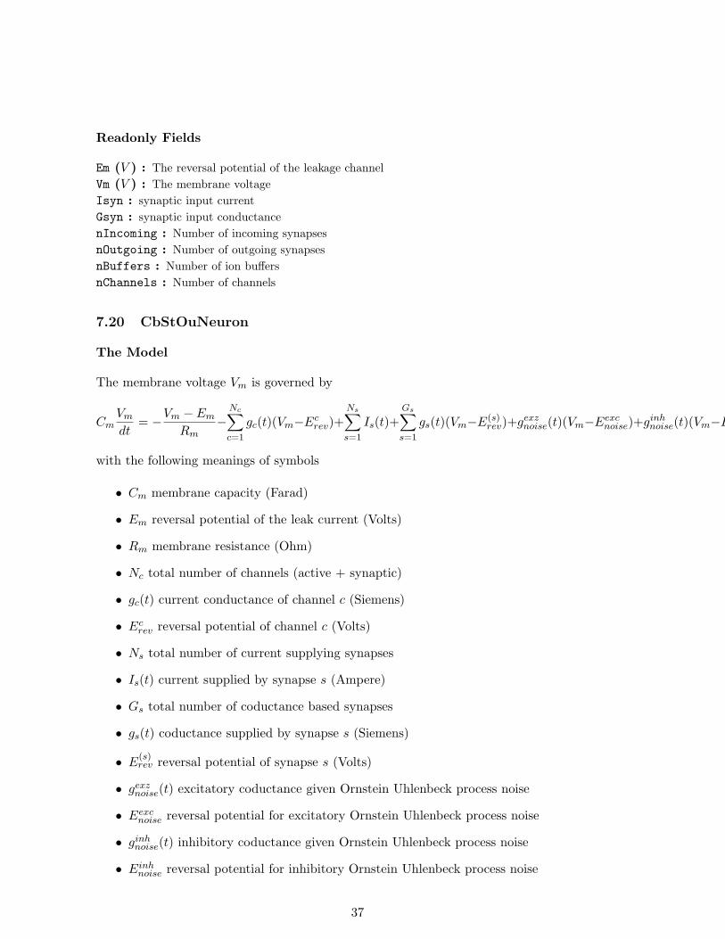
7.20 CbStOuNeuron

The Model


CmVm

dt= −Vm − Em

Rm−

Nc∑c=1

gc(t)(Vm−Ecrev)+

Ns∑s=1

Is(t)+Gs∑s=1

gs(t)(Vm−E(s)rev)+gexz

noise(t)(Vm−Eexcnoise)+ginh

noise(t)(Vm−Einhnoise)+Iinject













• gexznoise(t) excitatory coductance given Ornstein Uhlenbeck process noise

• Eexcnoise reversal potential for excitatory Ornstein Uhlenbeck process noise

• ginhnoise(t) inhibitory coductance given Ornstein Uhlenbeck process noise

• Einhnoise reversal potential for inhibitory Ornstein Uhlenbeck process noise

37





If the membrane voltage Vm exceeds the threshold Vtresh the CbNeuronSt sends a spike to allits outgoing synapses and the membrane voltage follows a predefined spike templageduring the absolute refractory period of length Trefract if doReset = 1.

If the flag doReset=0 the spike template is not applied and the above equation is also appliedduring the absolute refractory period but the event of threshold crossing is transmitted as aspike to outgoing synapses. This is usfull if one includes channels which produce a real actionpotential (see HH K Channel and HH Na Channel) but one still just wants to communicatethe spikes as events in time.

Implementation



ge (S) : exc and inh conductances (noise)gi (S) : exc and inh conductances (noise)ge0 (S) : exc and inh mean conductances (noise)gi0 (S) : exc and inh mean conductances (noise)tau e (S) : time constants and std for exc and inh conductances (noise)tau i (S) : time constants and std for exc and inh conductances (noise)sig e (S) : time constants and std for exc and inh conductances (noise)sig i (S) : time constants and std for exc and inh conductances (noise)Ee (V ) : Reversal potential for exc and inh currents (noise)Ei (V ) : Reversal potential for exc and inh currents (noise)STempHeight (V olt) : HeightVthresh (V ) : If Vm exceeds Vthresh a spike is emmited.Vreset (V ) : The voltage to reset Vm to after a spike.doReset (flag) : Flag which determines wheter Vm should be reseted after a spikeTrefract (sec) : Length of the absolute refractory period.nummethod (flag) : Numerical method for the solution of the differential equation: Exp. Euler =



Vresting (V ) : The resting membrane voltage.Vinit (V ) : Initial condition forVm at time t = 0.

38

VmScale (V ) : Defines the difference between Vresting and the Vthresh for the calculation of theiongate tables and the ionbuffer Erev.

Inoise (W 2) : Variance of the noise to be added each integration time constant.Iinject (A) : Constant current to be injected into the CB neuron.

Readonly Fields


7.21 CountSpikeFilter


time window : Length of time window.

Readonly Fields


7.22 DiscretizationPreprocessor

Readonly Fields

nInputRows : Number of rows for input vectors.nOutputRows : Number of rows for output vectors.

7.23 dNACNeuron

Uses AChannel Hoffman97

39







Readonly Fields


7.24 dNACOUNeuron

Uses AChannel Hoffman97


ge (S) : exc and inh conductances (noise)gi (S) : exc and inh conductances (noise)ge0 (S) : exc and inh mean conductances (noise)gi0 (S) : exc and inh mean conductances (noise)tau e (S) : time constants and std for exc and inh conductances (noise)tau i (S) : time constants and std for exc and inh conductances (noise)sig e (S) : time constants and std for exc and inh conductances (noise)sig i (S) : time constants and std for exc and inh conductances (noise)Ee (V ) : Reversal potential for exc and inh currents (noise)Ei (V ) : Reversal potential for exc and inh currents (noise)

40






Readonly Fields


7.25 DynamicSpikingCbSynapse

The conductance g(t) of the synapse is increased by W ·r ·u when a presynaptic spike hits thesynapse and decays exponentially (time constant τ ) otherwise. u and r model the currentstate of facilitation and depression.


E : Equilibrium potential given by the Nernst equation.U : The use parameter of the dynamic synapseD (sec) : The time constant of the depression of the dynamic synapseF (sec) : The time constant of the facilitation of the dynamic synapseu0 : Value of the time varying facilitation state variable u for the first spiker0 : Value of the time varying depression state variable r for the first spiketau (sec) : The synaptic time constant τ

W : The weight (scaling factor, strenght, maximal amplitude) of the synapsedelay (sec) : The synaptic transmission delay

41

Readonly Fields

u : The time varying state variable u for facilitationr : The time varying state variable u for depressionpsr : The psr (postsynaptic response) is the result of whatever computation is going on in a synapse.steps2cutoff :

7.26 DynamicSpikingSynapse

The time varying state x(t) of the synapse is increased by W · r · u when a presynaptic spikehits the synapse and decays exponentially (time constant τ ) otherwise. u and r model thecurrent state of facilitation and depression.


U : The use parameter of the dynamic synapseD (sec) : The time constant of the depression of the dynamic synapseF (sec) : The time constant of the facilitation of the dynamic synapseu0 : Value of the time varying facilitation state variable u for the first spiker0 : Value of the time varying depression state variable r for the first spiketau (sec) : The synaptic time constant τ


Readonly Fields


7.27 DynamicStdpSynapse

See DynamicSpikingSynapse and StdpSynapse for details


U : The use parameter of the dynamic synapseD (sec) : The time constant of the depression of the dynamic synapseF (sec) : The time constant of the facilitation of the dynamic synapseu0 : Value of the time varying facilitation state variable u for the first spiker0 : Value of the time varying depression state variable r for the first spikeback delay (sec) : Delay of dendritic backpropagating spike (the synapse sees the postsynaptic

spike delayed by back delay

42

tauspost : Used for extended rule by Froemke and Dan. See Froemke and Dan (2002). Spike-timing-dependent synaptic modification induced by natural spike trains. Nature 416 (3/2002).

tauspre : Used for extended rule by Froemke and Dan.taupos : Timeconstant of exponential decay of positive learning window for STDP.tauneg : Timeconstant of exponential decay of negative learning window for STDP.dw :STDPgap : No learning is performed if |Delta| = |tpost − tpre| < STDPgap.activeSTDP : Set to 1 to activate STDP-learning. No learning is performed if set to 0.useFroemkeDanSTDP : activate extended rule by Froemke and Dan (default=1)Wex : The maximal/minimal weight of the synapseAneg : Defines the peak of the negative exponential learning window.Apos : Defines the peak of the positive exponential learning window.mupos : Extended multiplicative positive update: dw = (Wex − W )mupos ∗ Apos ∗

exp(−Delta/taupos). Set to 0 for basic update. See Guetig, Aharonov, Rotter and Sompolinsky(2003). Learning input correlations through non-linear asymmetric Hebbian plasticity. Journalof Neuroscience 23. pp.3697-3714.

muneg : Extended multiplicative negative update: dw = Wmupos ∗Aneg ∗ exp(Delta/tauneg). Set to0 for basic update.

tau (sec) : The synaptic time constant τ


Readonly Fields


7.28 ExpSpikeFilter


m tau1 : Time constant.

Readonly Fields


43

7.29 ExtInputNeuron


Vresting (V ) : The resting membrane voltage.Inoise (A2) : The noise of analog neuronstype : Type (e.g. inhibitory or excitatory) of the neuronmyIndex : ID of external input (is equal index of array)beReal : Flag if external input is used or normal input

Readonly Fields


7.30 ExtOutLifNeuron


myIndex : ID of external input (is equal index of array)beReal : Flag if external input is used or normal inputCm (F ) : The membrane capacity Cm


Vthresh (V ) : If Vm exceeds Vthresh a spike is emmited.Vresting (V ) : The resting membrane voltage.Vreset (V ) : The voltage to reset Vm to after a spike.Vinit (V ) : The initial condition for Vm at time t = 0.Trefract (sec) : The length of the absolute refractory period.Inoise (A) : The standard deviation of the noise to be added each integration time constant.Iinject (A) : A constant current to be injected into the LIF neuron.type : Type (e.g. inhibitory or excitatory) of the neuron

Readonly Fields

Isyn : synaptic input currentnIncoming : Number of incoming synapsesnOutgoing : Number of outgoing synapsesVm (V ) : The membrane voltage Vm

44

7.31 ExtOutLinearNeuron


Iinject (W ) : external current injected into neuronVinit (V ) : initial ’membrane voltage’Vresting (V ) : The resting membrane voltage.Inoise (A2) : The noise of analog neuronstype : Type (e.g. inhibitory or excitatory) of the neuronmyIndex : ID of external input (is equal index of array)beReal : Flag if external input is used or normal input

Readonly Fields


7.32 ExtOutSigmoidalNeuron


thresh (W ) : Itot = logsig(beta*(Itot-thresh))beta (1) : Itot = logsig(beta*(Itot-thresh))tau m : time constantA max (1) : the output of a sig neuron is scaled to (0,W max)I inject (W ) : external current injected into neuronVm init (V ) : initial ’membrane voltage’Vresting (V ) : The resting membrane voltage.Inoise (A2) : The noise of analog neuronstype : Type (e.g. inhibitory or excitatory) of the neuronmyIndex : ID of external input (is equal index of array)beReal : Flag if external input is used or normal input

Readonly Fields


7.33 GaussianAnalogFilter


m std dev : Standard deviation of the filter mask.nKernelLength : The length of the kernel.

45

Readonly Fields

nChannels : Number of Input channels to filter.

7.34 GVD cT Gate


Vh (V olt) : Inflection point of the sigmoidal function p(V )Vc (V olt) : Slope of the sigmoidal function p(V )Ts : Voltage independent time constant τ

nummethod (flag) : Numerical method for the solution of the differential equation: Exp. Euler =0, Crank-Nicolson = 1

k (1) : The exponent of the gatep : The state variable.

Readonly Fields


7.35 GVD Gate


Vh (V olt) : Inflection point of the sigmoidal function p(V )Vc (V olt) : Determines the slope of the sigmoidal function p(V )Ts : Scale of the time constant τ(V )Te : Additional exponential factor of the time constant τ(V )nummethod (flag) : Numerical method for the solution of the differential equation: Exp. Euler =

0, Crank-Nicolson = 1k (1) : The exponent of the gatep : The state variable.

Readonly Fields


7.36 HChannel Stuart98

Uses HnGate Stuart98

Reference: Stuart G, Spruston N. Determinants of voltage attenuation in neocortical pyra-midal neuron dendrites. J Neurosci. 1998 May 15;18(10):3501-10.

46



Readonly Fields


7.37 HH K Channel

Uses the gate HH n Gate



Readonly Fields


7.38 HH Na Channel

Uses the gates HH h Gate and HH m Gate



Readonly Fields


7.39 HHNeuron

The model is based on a CbNeuron and includes the HH K Channel and HH Na Channel foraction potetial generation.

47







Readonly Fields


7.40 HVACAChannel Brown93

Uses HVACAuGate Brown93 and HVACAvGate Brown93

Reference: Brown AM, Schwindt PC, Crill WE. Voltage dependence and activation kinetics ofpharmacologically defined components of the high-threshold calcium current in rat neocorticalneurons. J Neurophysiol. 1993 Oct;70(4):1530-43.

See also: Seamans JK, Durstewitz D, Christie BR, Stevens CF, Sejnowski TJ. DopamineD1/D5 receptor modulation of excitatory synaptic inputs to layer V prefrontal cortex neurons.Proc Natl Acad Sci U S A. 2001 Jan 2;98(1):301-6.



48

Readonly Fields


7.41 IfbNeuron

see Izhikevich E. ”Which modell to use for cortical spiking neurons?”

Model

A leaky-integrate-and-fire-or burst neuron model is implemented where the membrane poten-tial Vm of a neuron is given by

τmdVm

dt= −(Vm − Vresting) + Rm · (Isyn(t) + Iinject + Inoise)

where τm = Cm ·Rm is the membrane time constant, Rm is the membrane resistance, Isyn(t)is the current supplied by the synapses, Iinject is a non-specific background current and Inoise

is a Gaussion random variable with zero mean and a given variance noise.

At time t = 0 Vm ist set to Vinit . If Vm exceeds the threshold voltage Vthresh it is reset toVreset and hold there for the length Trefract of the absolute refractory period.

Implementation



Cm (F ) : The membrane capacity Cm


Vthresh (V ) : If Vm exceeds Vthresh a spike is emmited.Vresting (V ) : The resting membrane voltage.Vreset (V ) : The voltage to reset Vm to after a spike.Vinit (V ) : The initial condition for Vm at time t = 0.Trefract (sec) : The length of the absolute refractory period.Inoise (A) : The standard deviation of the noise to be added each integration time constant.Iinject (A) : A constant current to be injected into the LIF neuron.h : internal parameter h - deinactivation of Ca-channelstau p : tau p time constant for recovery from inactivationtau m : tau m time constant for inactivationVh : Vh constant for onset of Ca-channel activation.gh : gh constant for relative impact of Ca-current to leak current (0.5-2)type : Type (e.g. inhibitory or excitatory) of the neuron

49

Readonly Fields

Vm (V ) : The membrane voltage Vm

Isyn : synaptic input currentnIncoming : Number of incoming synapsesnOutgoing : Number of outgoing synapses

7.42 Izhi Neuron

see Izhikevich E. ”Simple model of Spiking Neurons”

Model

A canonical neuron model is implemented where the membrane potential Vm of a neuron isgiven by

, Rm is the membrane resistance, Isyn(t) is the current supplied by the synapses, Iinject isa non-specific background current and Inoise is a Gaussion random variable with zero meanand a given variance noise.


Implementation

The simple Euler method is used for numerical integration.




Vthresh (V ) : If Vm exceeds Vthresh a spike is emmited.Vresting (V ) : The resting membrane voltage.Vreset (V ) : The voltage to reset Vm to after a spike.Vinit (V ) : The initial condition for Vm at time t = 0.Trefract (sec) : The length of the absolute refractory period.Inoise (A) : The standard deviation of the noise to be added each integration time constant.Iinject (A) : A constant current to be injected into the LIF neuron.a : A constant (0.02, 01) describing the coupling of variable u to Vm;.b : A constant controlling sensitivity og u.c : A constant controlling reset of Vm (1000*Vreset).d : A constant controlling reset of u.type : Type (e.g. inhibitory or excitatory) of the neuron

50

Readonly Fields


Vb : The membrane voltage in millivolt.Vint : The membrane voltage in millivolt.u : internal variableub : The internal variable u adapted to millivolt and millisecond.Isyn : synaptic input currentnIncoming : Number of incoming synapsesnOutgoing : Number of outgoing synapses

7.43 KCAChannel Mainen96

Uses KCAnGate Mainen96

Reference: Mainen ZF, Sejnowski TJ. Influence of dendritic structure on firing pattern inmodel neocortical neurons. Nature. 1996 Jul 25;382(6589):363-6.



Readonly Fields


7.44 KChannel Korngreen02

Uses KnGate Korngreen02 and KlGate Korngreen02

Reference: Korngreen A, Sakmann B.Voltage-gated K+ channels in layer 5 neocortical pyra-midal neurones from young rats: subtypes and gradients. J Physiol. 2000 Jun 15;525 Pt3:621-39.



Readonly Fields


51

7.45 LifBurstNeuron

that produces bursts dependent on two additional variables analog to the implementation ofdynamical synapses: see Kaske&Bertschinger ”Traveling wave patterns...”

Model

A nonstandard leaky-integrate-and-fire neuron model is implemented where the membranepotential Vm of a neuron is given by

τmdVm



is a Gaussion random variable with zero mean and a given variance noise. Vreset is modulatedby u and r to produce spiking dependent on the previous spike pattern At time t = 0 Vm istset toVinit . If Vm exceeds the threshold voltageVthresh it is reset to Vreset and hold there forthe length Trefract of the absolute refractory period.

Implementation





Vthresh (V ) : If Vm exceeds Vthresh a spike is emmited.Vresting (V ) : The resting membrane voltage.Vreset (V ) : The default voltage to reset Vm to after a spike.VBthresh (V ) : spike pattern dependent treshold Vm to after a spike.Vinit (V ) : The initial condition for Vm at time t = 0.Trefract (sec) : The length of the absolute refractory period.Inoise (A) : The standard deviation of the noise to be added each integration time constant.Iinject (A) : A constant current to be injected into the LIF neuron.uB : internal parameter uB - recovery from spike facilitation with time constant FBrB : internal parameter rB - recovery from spike depression with time constant DBFB : FB time constant for recovery from facilitation of spike generation.DB : DB time constant for recovery from depression of spike generation.UB : UB constant for onset of facilitation of spike generation.type : Type (e.g. inhibitory or excitatory) of the neuron

Readonly Fields


Isyn : synaptic input currentnIncoming : Number of incoming synapsesnOutgoing : Number of outgoing synapses

52

7.46 LifNeuron

Model

A standard leaky-integrate-and-fire neuron model is implemented where the membrane po-tential Vm of a neuron is given by

τmdVm



is a Gaussion random variable with zero mean and a given variance noise.


Implementation





Vthresh (V ) : If Vm exceeds Vthresh a spike is emmited.Vresting (V ) : The resting membrane voltage.Vreset (V ) : The voltage to reset Vm to after a spike.Vinit (V ) : The initial condition for Vm at time t = 0.Trefract (sec) : The length of the absolute refractory period.Inoise (A) : The standard deviation of the noise to be added each integration time constant.Iinject (A) : A constant current to be injected into the LIF neuron.type : Type (e.g. inhibitory or excitatory) of the neuron

Readonly Fields

Isyn : synaptic input currentnIncoming : Number of incoming synapsesnOutgoing : Number of outgoing synapsesVm (V ) : The membrane voltage Vm

7.47 linear classification


nClasses : Number of Classes.range low : Lower bound of algorithms range.range high : Upper bound of algorithms range.

53

Readonly Fields

nInputRows : Number of rows for input vectors.

7.48 LinearNeuron


Iinject (W ) : external current injected into neuronVinit (V ) : initial ’membrane voltage’Vresting (V ) : The resting membrane voltage.Inoise (A2) : The noise of analog neuronstype : Type (e.g. inhibitory or excitatory) of the neuron

Readonly Fields


7.49 LinearPreprocessor

Readonly Fields


7.50 linear regression


range low : Lower bound of algorithms range.range high : Upper bound of algorithms range.

Readonly Fields

nInputRows : Number of rows for input vectors.

7.51 MChannel Mainen96

Uses MnGate Mainen96

Reference: Mainen ZF, Sejnowski TJ. Influence of dendritic structure on firing pattern inmodel neocortical neurons. Nature. 1996 Jul 25;382(6589):363-6.

54



Readonly Fields


7.52 MChannel Wang98

From: Wang, H.-S., Pan, Z., Shi, W., Brown, B. S., Wymore, R.S., Cohen, I. S., Dixon, J.E. and McKinnon, D. (1998) KCNQ2 and KCNQ3Potassium Channel Subunits: MolecularCorrelates of the M-Channel. Science, 282, 1890-1893



Readonly Fields


7.53 Mean Std Preprocessor

Every row x i of the input vector is transformed into x′i = (xi − mi)/stdi , where m i and

std i are the mean and standard deviation of the i-th row.

Readonly Fields


7.54 MexRecorder


commonChannels : Flag: 1 ... output all channels in one matrix (WARNING: no spikes are returnedyet), 0 ... output each recorded field as seperate channel

dt (sec) : The timestep at which an recording should be done (no meaning if recording spikes).Tprealloc (sec) : Provide your best guess how long the network will be simulated (in simulation

time).enabled : Flag: 0 ... recorder disabled, 1 ... recoder enabled

55

7.55 NPChannel McCormick02

Uses NPmGate McCormick92

Reference: McCormick DA, Huguenard JR. A model of the electrophysiological properties ofthalamocortical relay neurons. J Neurophysiol 1992 Oct;68(4):1384-400

See also: Alexander D. Protopapas, Michael Vanier and James M. Bower. Chapter 12:”Simulating Large Networks of Neurons” in Methods in Neuronal Modeling: From Ions toNetworks, 2nd edition, Christof Koch and Idan Segev, eds, MIT Press, Cambridge, Mass.,1998



Readonly Fields


7.56 PCAPreprocessor

Readonly Fields


7.57 Readout

This class implements readouts within the simulation. Readouts take the responses of theliquid and calculate a new function with these inputs. Readouts can be trained to approximatesome target function. Readouts can be connected to physical models or feedback neurons forclosed-loop simulations. Therefore the interface of readouts is similar to that of synapses.The output of a readout can be recorded.


enabled : Flag: 0 ... readout disabled, 1 ... readout enabledoffset : Offset of output values.range : Range of output values.

Readonly Fields

output : Output variable of a readout.

56

7.58 Recorder

This class allows you to record traces of any fields of any object during the simulation. Therecorded traces of an Recorder with handle rec idx can be obtained via

R=csim(’get’,rec_idx,’traces’);

The ecxact form of R depends on the flag commonChannels (see below). Note that the tracesreturned always start at time $t=0$ and are recorded at an interval of dt.

In addition a recorder can also record spikes from spike emitting objects. Via a commandlike

csim(’connect’,rec_idx,neuron_idx,’spikes’);

the Recorder with handle rec idx is set up to record the spikes form the spike emittingobjects with handles neuron idx.

commonChannels=0 In this case the Matlab array R is a struct array with the only fieldchannel which is in turn a struct array with the following fields:

• R.channel(j).idx : handle of the object from which field the data was recorded

• R.channel(j).spiking : binary flag (0/1) which determines if data should be interpretedas spike times or as an analog signal

• R.channel(j).dt : time discretization; for analog signals only

• R.channel(j).data : signal data : vector of the analog values or spike times.

• R.channel(j).fieldName : name of the recorded field

commonChannels=1 In this case ∗∗R has two fields (WARNING: no spikes are returned):

• R.data : A double array where R.data(j,s) is the s -th recorded value of the j -thfield.

• R.info : A struct array where R.info(j).idx is the handle of the object from whichthe field R.info(j).fieldName is recorded.


commonChannels : Flag: 1 ... output all channels in one matrix (WARNING: no spikes are returnedyet), 0 ... output each recorded field as seperate channel

dt (sec) : The timestep at which an recording should be done (no meaning if recording spikes).Tprealloc (sec) : Provide your best guess how long the network will be simulated (in simulation

time).enabled : Flag: 0 ... recorder disabled, 1 ... recoder enabled

57

7.59 SICChannel Maciokas02

Uses SICmGate Maciokas02 and SIChGate Maciokas02

Reference: Maciokas, J., Goodman, P., Kenyon, J., Accurate Dynamical Model of Interneu-ronal GABAergic Channel Physiologies



Readonly Fields


7.60 SigmoidalNeuron


thresh (W ) : Itot = logsig(beta*(Itot-thresh))beta (1) : Itot = logsig(beta*(Itot-thresh))tau m : time constantA max (1) : the output of a sig neuron is scaled to (0,W max)I inject (W ) : external current injected into neuronVm init (V ) : initial ’membrane voltage’Vresting (V ) : The resting membrane voltage.Inoise (A2) : The noise of analog neuronstype : Type (e.g. inhibitory or excitatory) of the neuron

Readonly Fields


7.61 SpikingInputNeuron


type : Type (e.g. inhibitory or excitatory) of the neuron

Readonly Fields

nIncoming : Number of incoming synapsesnOutgoing : Number of outgoing synapses

58

7.62 SpikingTeacher

7.63 StaticAnalogCbSynapse


E : Equilibrium potential given by the Nernst equation.Inoise : The noise of our analog synapsesW : The weight (scaling factor, strenght, maximal amplitude) of the synapsedelay (sec) : The synaptic transmission delay

Readonly Fields

psr : The psr (postsynaptic response) is the result of whatever computation is going on in a synapse.

7.64 StaticAnalogSynapse


Inoise : The noise of our analog synapsesW : The weight (scaling factor, strenght, maximal amplitude) of the synapsedelay (sec) : The synaptic transmission delay

Readonly Fields

psr : The psr (postsynaptic response) is the result of whatever computation is going on in a synapse.

7.65 StaticSpikingCbSynapse

We call a synapse a static synapse if the amplitude of each evoked conductance change isequal. Here we implement a conductance g(t) of the form g(t) = W · exp(−t/τ) for each spikewhich hits the synapse at time t with an amplitude of W and a decay time constant of τ .The responses of all the spikes are added up linearly.


E : Equilibrium potential given by the Nernst equation.tau (sec) : The synaptic time constant τ


Readonly Fields

psr : The psr (postsynaptic response) is the result of whatever computation is going on in a synapse.steps2cutoff :

59

7.66 StaticSpikingSynapse

We call a synapse a static synapse if the amplitude of each postsynaptic response is equal.Here we implement a synaptic response x(t) of the form x(t) = W · exp(−t/τ) for each spikewhich hits the synapse at time t with an amplitude of W and a decay time constant of τ .The responses of all the spikes are added up linearly.




Readonly Fields


7.67 StaticStdpSynapse


back delay (sec) : Delay of dendritic backpropagating spike (the synapse sees the postsynapticspike delayed by back delay

tauspost : Used for extended rule by Froemke and Dan. See Froemke and Dan (2002). Spike-timing-dependent synaptic modification induced by natural spike trains. Nature 416 (3/2002).

tauspre : Used for extended rule by Froemke and Dan.taupos : Timeconstant of exponential decay of positive learning window for STDP.tauneg : Timeconstant of exponential decay of negative learning window for STDP.dw :STDPgap : No learning is performed if |Delta| = |tpost − tpre| < STDPgap.activeSTDP : Set to 1 to activate STDP-learning. No learning is performed if set to 0.useFroemkeDanSTDP : activate extended rule by Froemke and Dan (default=1)Wex : The maximal/minimal weight of the synapseAneg : Defines the peak of the negative exponential learning window.Apos : Defines the peak of the positive exponential learning window.mupos : Extended multiplicative positive update: dw = (Wex − W )mupos ∗ Apos ∗

exp(−Delta/taupos). Set to 0 for basic update. See Guetig, Aharonov, Rotter and Sompolinsky(2003). Learning input correlations through non-linear asymmetric Hebbian plasticity. Journalof Neuroscience 23. pp.3697-3714.

muneg : Extended multiplicative negative update: dw = Wmupos ∗Aneg ∗ exp(Delta/tauneg). Set to0 for basic update.



60

Readonly Fields


7.68 Traubs HH K Channel

Used in the TraubsHHNeuron neuron model.

Uses the gate Traubs HH n Gate

gKd = 0.03 S/cm2 EK = -90 mV



Readonly Fields


7.69 Traubs HH Na Channel

Used in the TraubsHHNeuron neuron model.

Uses the gates Traubs HH h Gate and Traubs HH m Gate.

gNa = 0.1 S/cm2 ENa = 50 mV



Readonly Fields


7.70 TraubsHHNeuron

This model is a modified version of Traub’s model of Na/K currents for action potentials inhippocampal pyramidal cells, which was modified from HH equations to fit the kinetics ofthose neurons; the rate constants correspond to a temperature of 36 deg C

The model is based on a CbNeuron and includes the Traubs HH K Channel and Traubs -HH Na Channel for action potetial generation.

INa = gNa ∗ m∧3 ∗ h ∗ (v-ENa) IKd = gKd ∗ n∧4 ∗ (v-EK)

61

m’ = (m inf - m) / tau m h’ = (h inf - h) / tau h n’ = (n inf - n) / tau n

v2 = v - Vtr

alpha m = 0.32 ∗ (13-v2) / ( exp((13-v2)/4) - 1) beta m = 0.28 ∗ (v2-40) / ( exp((v2-40)/5)- 1) tau m = 1 / (alpha m + beta m) m inf = alpha m / (alpha m + beta m)

alpha h = 0.128 ∗ exp((17-v2)/18) beta h = 4 / ( 1 + exp((40-v2)/5) ) tau h = 1 / (alpha h+ beta h) h inf = alpha h / (alpha h + beta h)

alpha n = 0.032 ∗ (15-v2) / ( exp((15-v2)/5) - 1) beta n = 0.5 ∗ exp((10-v2)/40) tau n = 1/ (alpha n + beta n) n inf = alpha n / (alpha n + beta n)

HH parameters:

gNa = 0.1 S/cm2 gKd = 0.03 S/cm2 ENa = 50 mV EK = -90 mV Vtr = -63 mV (adjuststhreshold to around -50 mV)







Readonly Fields


62

7.71 TriangularAnalogFilter


nKernelLength : The length of the kernel.

Readonly Fields


7.72 UserAnalogFilter


m weights : User-defined weights.nKernelLength : The length of the kernel.

Readonly Fields


References

[Dayan and Abbott, 2001] Dayan, P. and Abbott, L. (2001). Theoretical Neuroscience:Computational and Mathematical Modeling of Neural Systems. MIT Press. See alsohttp://people.brandeis.edu/~abbott/book/.

[Gerstner and Kistler, 2002] Gerstner, W. and Kistler, W. (2002). Spiking Neuron Models.Cambridge University Press. See also http://diwww.epfl.ch/~gerstner/BUCH.html.

63

http://people.brandeis.edu/~abbott/book/

http://diwww.epfl.ch/~gerstner/BUCH.html

Documents

Version 1.1 User Manual - Graz University of Technology · 1.3 Features of the current version Different levels of modeling Different neuron models: leaky-integrate-and-fire neurons,