Embed Size (px)
Citation preview

FEMAPGetting Started
Version 11.1
MUF1000-GS-103

Proprietary and Restricted Rights Notice
This software and related documentation are proprietary to Siemens Product Lifecycle Management Software Inc.
© 2013 Siemens Product Lifecycle Management Software Inc. All Rights Reserved.
Siemens and the Siemens logo are registered trademarks of Siemens AG. NX is a trademark or registered trade-mark of Siemens Product Lifecycle Management Software Inc. or its subsidiaries in the United States and in other countries. All other trademarks, registered trademarks or service marks belong to their respective holders.
The following copyright refers only to the “bmp2raster.exe” executable distributed with FEMAP:
NeuQuant Neural-Net Quantization Algorithm
Copyright (c) 1994 Anthony Dekker
NEUQUANT Neural-Net quantization algorithm by Anthony Dekker, 1994.
See "Kohonen neural networks for optimal colour quantization" in "Network: Computation in Neural Systems" Vol. 5 (1994) pp 351-367 for a discussion of the algorithm.
See also http://members.ozemail.com.au/~dekker/NEUQUANT.HTML
Any party obtaining a copy of these files from the author, directly or indirectly, is granted, free of charge, a full and unrestricted irrevocable, world-wide, paid up, royalty-free, nonexclusive right and license to deal in this software and documentation files (the "Software"), including without limitation the rights to use, copy, modify, merge, pub-lish, distribute, sublicense, and/or sell copies of the Software, and to permit persons who receive copies from any such party to do so, with the only requirement being that this copyright notice remain intact.
Siemens PLM
Web: http://www.femap.com
Customer Support
Phone: (714) 952-5444, (800) 955-0000 (In US & Canada)
Web: http://support.ugs.com

Conventions This manual uses different fonts to highlight command names or input that you must type.
Throughout this manual, you will see references to Windows. Windows refers to Microsoft® Windows XP, Win-dows Vista, and Windows 7 (32-bit and 64-bit versions). You will need one of these operating environments to run FEMAP for the PC. This manual assumes that you are familiar with the general use of the operating environment. If you are not, you can refer to the Windows User’s Guide for additional assistance.
Similarly, throughout the manual all references to FEMAP, refer to the latest version of our software.
a:setup Shows text that you should type.
OK, Cancel Shows a command name or text that you will see in a dialog box.


FEMAP Examples
Proprietary and Restricted Rights Notice1. Introduction
Introduction to FEMAP . . . . . . . . . . . . . . . . . . . . 1-1Using the FEMAP Examples Guide . . . . . . . . . . . . . . . . . 1-3The FEMAP Documentation Set . . . . . . . . . . . . . . . . . . 1-5
2. Installing FEMAPHardware/Software Requirements . . . . . . . . . . . . . . . . . . 2-1Installation - Stand Alone . . . . . . . . . . . . . . . . . . . 2-2Network Installation . . . . . . . . . . . . . . . . . . . . 2-5Starting FEMAP . . . . . . . . . . . . . . . . . . . . . 2-8Improving Performance (RAM Management) . . . . . . . . . . . . . . 2-11Licensing Conversion Methods . . . . . . . . . . . . . . . . . 2-12
What’s New in FEMAP What’s New for version 11.1
User Interface . . . . . . . . . . . . . . . . . . . . . . 3-3Model Merge . . . . . . . . . . . . . . . . . . . . . . 3-5Geometry . . . . . . . . . . . . . . . . . . . . . . 3-8Meshing . . . . . . . . . . . . . . . . . . . . . . 3-14Elements . . . . . . . . . . . . . . . . . . . . . . 3-15Materials . . . . . . . . . . . . . . . . . . . . . . 3-16Properties . . . . . . . . . . . . . . . . . . . . . 3-16Loads and Constraints . . . . . . . . . . . . . . . . . . . 3-17Connections (Region, Properties, and Connectors) . . . . . . . . . . . . . 3-22Groups and Layers . . . . . . . . . . . . . . . . . . . . 3-23Views . . . . . . . . . . . . . . . . . . . . . . 3-23Output and Post-Processing . . . . . . . . . . . . . . . . . . 3-24Geometry Interfaces . . . . . . . . . . . . . . . . . . . 3-28Analysis Program Interfaces . . . . . . . . . . . . . . . . . . 3-29Tools . . . . . . . . . . . . . . . . . . . . . . 3-33OLE/COM API . . . . . . . . . . . . . . . . . . . . 3-38Preferences . . . . . . . . . . . . . . . . . . . . . 3-40
3. Analyzing Buckling for a BracketImporting the Geometry . . . . . . . . . . . . . . . . . . . . 4-1Meshing the Model . . . . . . . . . . . . . . . . . . . . . 4-2Applying Constraints and Loads . . . . . . . . . . . . . . . . . . 4-8Post-processing the Results . . . . . . . . . . . . . . . . . . 4-13
4. Analyzing a Beam ModelImporting the Geometry . . . . . . . . . . . . . . . . . . . . 5-1Defining the Material and Property . . . . . . . . . . . . . . . . . 5-2Meshing the Model . . . . . . . . . . . . . . . . . . . . . 5-5Applying Constraints and Loads . . . . . . . . . . . . . . . . . 5-12Analyzing the Model . . . . . . . . . . . . . . . . . . . 5-16Post-Processing the Results . . . . . . . . . . . . . . . . . . 5-17
5. Analyzing a Midsurface Model of an Electrical BoxImporting the Geometry . . . . . . . . . . . . . . . . . . . . 6-1Creating the Midsurface Model . . . . . . . . . . . . . . . . . . 6-2Meshing the Model . . . . . . . . . . . . . . . . . . . . . 6-8Applying Loads and Constraints . . . . . . . . . . . . . . . . . 6-10Analyzing the Model . . . . . . . . . . . . . . . . . . . 6-12Post-processing the Results . . . . . . . . . . . . . . . . . . 6-13
6. Analysis of a Simple Assembly

TOC-2
Importing the Geometry . . . . . . . . . . . . . . . . . . . 7-1Creating Connections . . . . . . . . . . . . . . . . . . . . 7-2Applying Loads and Constraints. . . . . . . . . . . . . . . . . . 7-8Meshing the Model . . . . . . . . . . . . . . . . . . . . 7-14Analyzing the “Glued Contact” Model . . . . . . . . . . . . . . . . 7-16Post-processing the Results of “Glued Contact” Analysis . . . . . . . . . . . . . 7-17Modifying the Connection Property . . . . . . . . . . . . . . . . . 7-18Applying additional Constraints for stability . . . . . . . . . . . . . . . 7-22Analyzing the “Linear Contact” Model . . . . . . . . . . . . . . . . 7-23Post-processing the Results of “Linear Contact” Analysis. . . . . . . . . . . . . 7-24

1. Introduction
This section introduces FEMAP and explains how to use the FEMAP Examples guide.
Introduction to FEMAPFEMAP is finite element modeling and post-processing software that allows you to perform engineering analyses both quickly and confidently. FEMAP provides the capability to develop sophisticated analyses of stress, temperature, and dynamic performance directly on the desktop. With easy access to CAD and office automation tools, productivity is dramat-ically improved compared to traditional approaches.
FEMAP automatically provides the integration that is necessary to link all aspects of your analysis. FEMAP can be used to create geometry, or you can import CAD geometry. FEMAP provides powerful tools for meshing geometry, as well as applying loads and boundary conditions. You may then use FEMAP to export an input file to over 20 finite element codes. FEMAP can also read the results from the solver program. Once results are obtained in FEMAP, a wide variety of tools are available for visualizing and reporting on your results.
With FEMAP you can:
• Import or Create Geometry
• Build a Finite Element Model
• Check Your Model
• Analyze Your Model
• Post-process Results
• Document Results
Import or Create GeometryFEMAP can directly import geometry from your CAD or design system. In fact, FEMAP can directly import a solid model from any ACIS-based or Parasolid-based modeling package. If your modeling package does not use either of these pack-ages, you can use the FEMAP IGES or STEP reader. If you are using I-DEAS, you can bring a single part into FEMAP by exporting a Viewer XML (IDI) file from I-DEAS. These files can be read and then stitched together to form a solid. This typically requires using one command.
If you do not have CAD geometry, you can create geometry directly in FEMAP using powerful wireframe and solid model-ing tools. Solid modeling directly in FEMAP uses the robust Parasolid modeling engine. You can build or modify solid models using the Parasolid engine, and then export the geometry out of FEMAP. This is very convenient if you need to export geometry to CAD packages that are Parasolid-based.
Build a Finite Element ModelRegardless of the origin of your geometry, you can use FEMAP to create a complete finite element model. Meshes can be created by many methods ranging from manual creation, to mapped meshing between keypoints, to fully automatic meshing of curves, surfaces and solids. FEMAP can even work with your existing analysis models. You can import and manipulate these models using the interfaces to any of the supported analysis programs.
Appropriate materials and section properties can be created or assigned from FEMAP libraries. Many types of constraint and loading conditions can be applied to represent the design environment. You can apply loads/constraints directly on finite element entities (nodes and elements), or you can apply them to geometry. FEMAP will automatically convert geometric conditions to nodal/elemental values upon translation to your solver program. You may even convert these loads before translation to convince yourself that the loading conditions are appropriate for your model.

1-2 Introduction
Check Your ModelAt every step of the modeling process, you receive graphical verification of your progress. You need not worry about mak-ing a mistake because FEMAP contains a multi-level undo and redo capability.
FEMAP also provides extensive tools for checking your model before you analyze it to give you the confidence that you have properly modeled your part. It constantly examines input to prevent errors in the model, and provides immediate visual feedback. FEMAP also provides a comprehensive set of tools to evaluate your finite element model and identify errors that are often not obvious. For example, FEMAP can check for coincident geometry, find improper connections, estimate mass and inertia, evaluate your constraint conditions, and sum your loading conditions. Each of these methods can be used to identify and eliminate potential errors, saving you considerable time and money.
Analyze Your ModelWhen your model is complete, FEMAP provides interface to over 20 popular programs to perform finite element analysis. You can even import a model from one analysis program and automatically convert it to the format for a different analysis program.
The NX Nastran for FEMAP solver is a general finite element analysis program for structural and thermal analysis that is integrated with FEMAP.
Post-process ResultsAfter your analysis, FEMAP provides both powerful visualization tools that enable you to quickly interpret results, and numerical tools to search, report, and perform further calculations using these results. Deformation plots, contour plots, ani-mations, and XY plots are just some of the post-processing tools available to the FEMAP user. FEMAP supports OpenGL, which provides even more capability for post-processing, including dynamic visualization of contours through solid parts. You can dynamically rotate solid contoured models with one push of your mouse button. Section cuts and isosurfaces can be viewed dynamically by simply moving your cursor.
Document ResultsDocumentation is also a very important factor with any analysis. FEMAP obviously provides direct, high quality printing and plotting of both graphics and text. Frequently, however, graphics or text must be incorporated into a larger report or pre-sentation. FEMAP can export both graphics and text to non-engineering programs with a simple Windows Cut command. You can easily export pictures to popular programs such as Microsoft Word, Microsoft Power Point, and Adobe Frame-maker. You can export to spreadsheets, databases, word processors, desktop publishing software, and paint and illustration programs. These links enable you to create and publish a complete report or presentation, all electronically, right on your desktop.
With support for AVI files, you can even include an animation directly in your Power Point Presentation or Word document. FEMAP also supports VRML and JPEG format so anyone can easily view results with standard viewers.

Using the FEMAP Examples Guide 1-3
Using the FEMAP Examples GuideThe FEMAP Examples guide is designed to teach new users the basics of using FEMAP. It contains a number of examples that take you step-by-step through the processes for building and using an FEA model.
Working through the ExamplesAs there are many different types of real analysis problems, there are different types of example problems shown here. Gen-erally, you should start with the first example in chapter 3 and work through the examples sequentially. Some of the later examples focus on specific techniques that you may not use in your work (beam modeling, axisymmetric modeling, midsur-facing). However, we recommend that you work through all the problems because they may contain some commands or techniques that you will find useful.
• Analyzing Buckling for a Bracket
• Analyzing a Beam Model
• Analyzing a Midsurface Model of an Electrical Box
• Analysis of a Simple Assembly
The examples in this manual should help you learn the basic FEA modeling process, general FEMAP commands, and the FEMAP command structure. For a more complete description of the FEMAP interface and modeling procedures, see the FEMAP User Guide. For an in-depth description of all the commands in FEMAP, see FEMAP Commands.

1-4 Introduction
Using the ExamplesIn general, italicized text identifies items in the user interface. For example: File, Preferences tells you to pick the File menu, then the Preferences command.
The Examples also include some graphics to help you identify user interface (UI) items. They include:
UI Graphic Meaning
Pick an option from a cascading menu.
Pick an item from a pull-down menu on a dialog box.
Pick an item from a list.
Pick an icon.
Enter a value into a field on a dialog box.
Pick a button.
Pick a radio button.
Check an item on or off in a dialog box.
Pick with the left mouse button.
Pick with the right mouse button.
Pick with middle mouse button if you have a three button mouse. Also can be the wheel of a wheel mouse.
Ctrl-A Hold the Control key, then pick the letter key.
F5 key Pick the function key.
Menu

The FEMAP Documentation Set 1-5
The FEMAP Documentation SetFEMAP comes with a set of three printed manuals: FEMAP Examples, the FEMAP User Guide, and the FEMAP Com-mands reference manual.
The FEMAP online help includes the contents of these manuals, as well as several additional books. The complete set includes:
• FEMAP Examples: Step-by-step examples for new users.
• FEMAP User Guide: General information on how to use FEMAP, including an overview of the finite element modeling process. Also contains reference information for the FEMAP analysis program and geometry interfaces.
• FEMAP Commands: Detailed information on how to use FEMAP commands.
• FEMAP API Reference: Information on how to write your own applications that work with FEMAP.
• What’s New: New features for this release.
When NX Nastran for FEMAP is installed, online help includes all of the above, as well as a full set of current NX Nastran documentation, to assist you during the solving portion of the analysis process.

1-6 Introduction

2. Installing FEMAP
This section will help you install and start using the FEMAP software.
This section contains information specific to getting started on a PC, which includes 32-bit and 64-bit versions of Windows XP, Windows Vista, and Windows 7.
A single DVD contains both the 32-bit version and 64-bit version of FEMAP. If you have a 32-bit system, you must install the 32-bit version. If you have a 64-bit system, you can choose to install either version, but will only get the benefits of using a 64-bit system by installing the 64-bit version.
Hardware/Software RequirementsThere are no special hardware/software requirements for FEMAP beyond those imposed by Windows operating systems. There are many types of hardware that will allow you to use FEMAP. Proper choice of hardware, however, can often make the difference between frustration and productivity. Here are a few suggestions:
• Memory, RAM
• Memory, (Hard Disk)
• Graphics Boards
• Browser
Memory, RAMYou will need at least 128 Mbytes of RAM to run FEMAP and the Parasolid solid modeling engine, which is the default. Obviously, the more amount of RAM the better. Adding RAM can be one of the most cost effective means of increasing per-formance.
If using the “Standard” geometry Engine in FEMAP, you can actually run with as little as 32 Mbytes of RAM. This is not a recommended configuration.
Memory, (Hard Disk)Required hard disk space is very difficult to estimate, but in general you will never have enough. Analysis results will be the main driver of any disk space requirement. Models are typically relatively small. A model with 1000 nodes and 1000 ele-ments would typically be less than 1 Mbyte in size. Output from an analysis of that model, however, could be 5 Mbytes, 10 Mbytes or even larger, depending on the output you request. To estimate total disk space, you need to first estimate how many models you will have online simultaneously, the approximate size of those models, and the type of output you will request.
Graphics BoardsStandard graphics adapters work very well with FEMAP. Specialized boards which contain support for OpenGL will pro-vide increased graphical performance when dynamically rotating large, complex models. They also usually provide higher resolution and more colors, which make graphics easier to see and more realistic.
BrowserTo run the online help, you should have Internet Explorer, version 6.0 or later. Browsers such as Mozilla Firefox may also be used to access the HTML help system.
Note: You MUST be logged in with Administrator privileges when installing FEMAP in order for the installation process to work properly.

2-2 Installing FEMAP
Installation - Stand AloneThis section describes the procedure that you should follow to install the stand alone (security device) version of FEMAP on your PC.
Security Device
In order to run the Stand Alone (Security Device) version of FEMAP a Rainbow SuperPro Parallel Port (pictured on left) or USB Port dongle is required. In order for your PC to be able to see the don-gle, a driver must first be installed. Installation of the driver requires Administrator privileges for your PC. During installation, if the current user has Administrator privileges, the installation pro-gram will automatically prompt for installation of this driver.
If the installer does not have Administrator privileges, someone with Administrator privileges will have to log in and install the driver manually. The driver installation program can be found in the
SentinalDriver directory of the FEMAP CD. On 32-bit and 64-bit Windows platforms, run CD\SentinalDriver\SPI750.exe. It is highly recommended that you do not have any security devices attached to your computer while you are installing the driver. Once the driver has been installed, you can plug a USB security device directly into an open USB port and it should be recognized. For the Parallel Port security device, it is highly recommended that you shut your computer down and turn it off before installing the security device. After it is installed, turn the computer on begin using FEMAP.
Setup Program ExecutionWindows XP/Vista/7
1. Log in to your computer as Administrator. As detailed above, this will make installation of the driver required to talk to the FEMAP dongle possible.
2. Insert the FEMAP CD into the drive. The setup should automatically begin within a few seconds. If it does not, manually run the SETUP.EXE program in the root directory of the FEMAP DVD.
Once setup is running you will see a license agreement. Assuming that you agree with the license agreement, choose “I accept the terms of the license agreement” and press Next to continue and select the directory where you would like to have the FEMAP program files installed.
You will be prompted for the selection of additional FEMAP options, please choose any optional modules and components that you wish to have installed.
FEMAP
Computer
Printer

Setup Program Execution 2-3
Notice that the installation will tell you the amount of disk space required for the chosen options to be installed and how much space is available on the drive where FEMAP will be installed.
The next dialog box allows you to Select FEMAP GUI Language. Select from English, German, Simplified Chinese, Tradi-tional Chinese, or Japanese then click Next.
You will now be asked which type of installation to perform. Choose Nodelocked Dongle as the licensing method.
After choosing Nodelocked Dongle and pressing Next, the program will be installed and then a driver required for the don-gle will automatically be installed. Finally, if you are installing FEMAP with the NX Nastran option you will be prompted to specify a “scratch” directory for the solver. You will need to have read/write access to this directory to be able to properly use NX Nastran.
FEMAP dongles are shipped good for 30 days from the first time they are run. In order to remove the time limit from your new FEMAP dongle, or upgrade an older dongle or network license, you must contact Siemens Product Lifecycle Manage-ment Software Inc. PLM's Global Technical Access Center (GTAC). In order to retrieve your FEMAP upgrade codes or your FLEXlm license file, you will need a GTAC WebKey account.
Note: If you plan on licensing FEMAP with a dongle (security key), not a network license, then you will probably want to UNCHECK the FLEXlm License Manager option as it is not used by the dongle.
Setup Type Description
Nodelocked Dongle - Rainbow SuperPro
Installs FEMAP for use with a Rainbow Parallel Port or USB don-gle. If you have the dongle version of FEMAP, choose this setup type.
Network Client - FLEXlm
Installs the Network Client version of FEMAP. This setup is for use where FEMAP is licensed via the FLEXlm license management software. With the Network Client version of FEMAP, one machine on your network will be designated as the license server. The fol-lowing “Network License Server” setup will have to be run on that machine.
Node-Limited Demo License
Installs the 300-Node demonstration version of FEMAP. This ver-sion requires no licensing, but is limited to very small models. It is intended for new users to try FEMAP and all its options.

2-4 Installing FEMAP
Obtaining a Webkey Account from Siemens Product Lifecycle Management Software Inc.
To request a WebKey account, access the web page; then provide the following information:
https://plmapps.ugs.com/webkey
• Your Installation ID
• WebKey Access Code
Your Installation ID is directly under the "sold to" information on your shipping order. For dongle-based FEMAP customers, your WebKey Access code is the unique portion of your FEMAP serial number, i.e. 3H-NT-1234, which is displayed in your current FEMAP in the Help - About dialog box, for this license as 1000-3H-NT-1234, with the version information at the beginning of the serial number removed. If you have any problems determining your Installation ID, FEMAP Serial Num-ber, or have trouble getting a WebKey account, please contact:
Trish McNamara - [email protected] - 610-458-6508, or
Mark Sherman - [email protected] - 610-458-6502
Obtaining Upgrade Codes or a new License File
1. Via the Web, using your WebKey Account -Upgrade codes or an updated license file can be e-mailed to you from the Customer Support (GTAC) web site http://support.ugs.com. In the Explore GTAC section, expand “License Management” and select “Current Licenses”. If prompted, enter WebKey and password. Click Passwords and License Files link. Select “Femap” as the Product and set Version to the appropriate version (i.e., 11.1 or 11.0). For LM Host or Dongle ID, enter either the unique portion of you FEMAP serial number (3H-NT-1234 in this case) if using a dongle or fill in the Ethernet address of your FEMAP license server if using FLEXlm network licenses. Your license or access codes will be e-mailed to the address supplied during WebKey registration.
2. Via the Phone - You can call GTAC at 714-952-5444 (US and Canada residents may use 800-955-0000) and enter option 1, 1, for your CSR or option 1,2, for Software Product Delivery (SPD). You should then request a copy of the license upgrade for a specific Installation ID and serial number or Ethernet Address.
For dongle versions of FEMAP, the information returned to you to upgrade the dongle will be in the form of two case insen-sitive alpha numeric codes. They will appear something like:
Access Code 1: 08aeca3f0f52639179
Access Code 2: 362ff63c3426d943
Use the Help, About command, then click the Security button. Cut and paste (to avoid errors) or type these two codes in to the appropriate fields and press OK. The FEMAP dongle is an EPROM, and these codes are used to update the memory of the dongle. Once these codes have been entered, you will never need to enter them again, with changes made to the memory of the dongle, they will either be useless, or simply write the same thing to memory again.

Network Installation 2-5
Network InstallationThe “Network Client” version of FEMAP utilizes the FLEXlm License Manager software from Flexera Software. This licensing approach requires some software to be installed on a server machine and other software to be installed on one or more clients. The clients then request and obtain licenses from the server. In a simple situation, both the client and server could be the same computer, but more likely they are different systems connected by a network.
Obtaining a License FileLicense files are obtained through the same procedure as defined above for getting the upgrade codes for a dongle license. Call GTAC, or use your WebKey account to request your FEMAP license file. The only difference in Net-work Licensed FEMAP is that you need to enter the LMHostID (Ethernet Address) of your license server when prompted instead of the FEMAP Serial Number. When you receive your license file information, you need to extract just the valid FLEXlm license entries, and copy them into a file called "license.dat". Please make sure that your license.dat looks something like the one show below. For FEMAP, you will have one SERVER line, one DAEMON line, and one or more FEATURE lines depending on how many options you have purchased with your FEMAP.
A couple of things to make sure of:
1. Make sure that the entry immediately following the word "SERVER" is the name of the license server where you are installing the license server software. If it is a temporary name, i.e. ANY, or THISHOST, change it to the cor-rect machine name. This is one of the two things in the license file that you can change.
2. Make sure that the third entry on the SERVER line matches the LMHostID of license server. This number is the key to the whole license file. If this does not match the LMHostID of the license server, then the licensing will not work.
3. The "DAEMON esplmd" line calls out the actual programs that hands out FEMAP licenses. If you have installed all the license server pieces in the same directory, it is fine as is. If the esplmd.exe program is not in the same direc-tory as LMTOOLS.EXE, you will have to edit this line to tell LMTOOLS.EXE where to find it. This is the other part of a license file that you can change.
License Server This section provides instructions on installing the network license manager and configuring your server.
Installing the FLEXlm License Manager
To begin the server installation, simply insert the FEMAP CD and allow it to AutoRun, or choose setup from the CD. FEMAP will ask which “features” should be installed. If you only want to install the license server, then UNCHECK all the options except “FLEXlm License Manager”. Once FEMAP has installed the software, copy
2-6 Installing FEMAP
your license file (usually called "license.dat") to the same directory where you installed the license server compo-nents.
Configuring the FLEXlm License Manager
You can run the LMTOOLS program from the FEMAP entry on your start -> All Programs - >FEMAP v11.1 -> FLEXlm License Manager, or manually run LMTOOLS.EXE from its installed directory.
Once LMTOOLS is running, select the “Config Services” Tab.
Fill in a Service Name, specify a path to the lmgrd.exe file (a required FLEXlm component) that can be found in the installation directory, and specify the path the license file. Finally, check the “Use Services” option, and then the “Start Server at Power Up”. Press the “Save Service” button.
Answer “Yes” to:
You must start the license server manually the first time, press the “Start/Stop/Reread” tab.
Configuring Network Client Machines 2-7
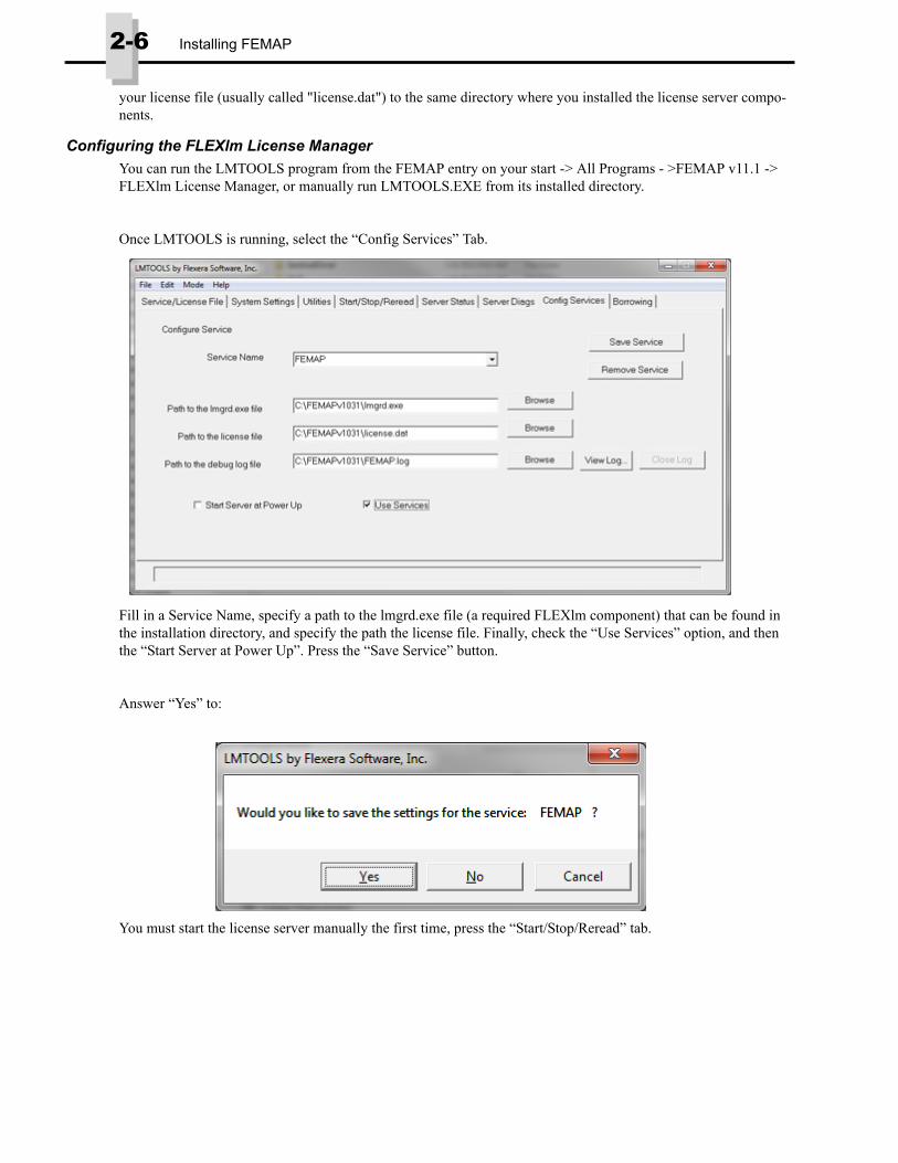
Select the FEMAP service that you just created, and press the “Start Server” button. At this point FLEXlm will be handing out FEMAP licenses on your network. To verify that everything is working fine from the license server standpoint, press the “Server Status” tab.
Press the “Perform Status Enquiry” button and the text window will be filled with status information about your FLEXlm license server. In the text window you will find information about how many licenses are available, and once user start checking out licenses, how many are in use
Configuring Network Client Machines Once your network license server is up and running, configuring FEMAP Network Client machines is very easy. Make sure that FEMAP is installed on the local machine using the "Network Client" setup type. To configure client machines to access the network license:
You have two options for telling network client machines how to find licenses on the license server:
1. Place a copy of the "license.dat" file in the FEMAP directory on the cli-ent machine. FEMAP will extract the name of the license server from the license file, and check out a license and run. The only drawback to this approach is that you must remember to update every copy of the license file when you receive a new one from Siemens PLM Software, Inc. (updates, licensing changes, etc.). To avoid this problem, you can type in the full network path to the License File in the “License File” field used below for HostName/IP Address location of the license server.
2. Tell FEMAP the name or IP address of the License Server.
a. Start FEMAP
b. Go to Help - About - Security
c. In the "License File" field, enter the name of the license server, preceded by an ampersand. In the example below, FEMAP is told to check out licenses from a network machine named PLSRV2:
d. In order for this machine name approach to work, the client computer must be able to see the license server com-puter via TCP/IP networking. To verify this, you can open a Command Prompt and ping the license server. In this case, one would type "ping PHLSRV2". The ping command will let you know if it can talk to the machine name indicated. If the client computer cannot find the license server by its name, you can also enter the IP address of the license server, preceded by an ampersand and licensing should also work.

2-8 Installing FEMAP
Monitoring Network UsageIn a multi-user environment, sometimes you will not be able to get a license simply because all available licenses are in use. You can find out who is using licenses, which computers they are using and when they started their license simply by going to Help, About, and pressing the Security button. At the bottom of the dialog box you will find information that will give you this information.
If you fail to get a license because none are available, you will not be able to work in FEMAP. You do not however, have to leave FEMAP. You can simply stay there and periodically try a command. Whenever a license becomes available it will be assigned to you and your command will succeed. If there are still no licenses available, you will simply get a message that says try again later.
Copying FEMAP from one machine to anotherIn previous versions, the FEMAP directory created from a proper installation could simply be copied from one machine to another, and then with the proper licensing, could be run on the new machine. For FEMAP 9.3.1 and above, there is one additional step which must be done in order for a copied version of FEMAP to be able to run.
Once the FEMAP directory has been copied, you need to go into the directory find an executable file called “vcre-dist_x86.exe”, then run the executable. This will install a set of Microsoft Compiler Libraries needed for FEMAP 9.3.1 to run properly.
On 64-bit operating systems, you will need to run “vcredist_x86.exe” and then run a 64-bit version of the execut-able called “vcredist_x64.exe”. You need to run both because FEMAP still uses some 32-bit applications in the 64-bit versions. For instance, the FEMAP Neutral File translators are all 32-bit applications.
Starting FEMAPThere are several command line options to launch FEMAP. The simplest method to launch FEMAP is to create a shortcut for FEMAP on your desktop and double-click the icon when you want to launch FEMAP. This will use the command line contained under the shortcut to launch FEMAP. You can modify this command line by right-clicking on the FEMAP icon, selecting properties, and changing the command line option on the shortcut.
The command line will contain the executable (and its path). After the femap.exe, there are several options which may be used to determine the mode in which FEMAP will operate. A list of these command line options are pro-vided below.
c:\FEMAPv###\femap.exe [-R] [-NEU] [-NOSPL] [-D dxf_file] [-N neu_file]
[-PRG program_file] [-SE Solid Edge_File] [-L port] [-SAT sat_file]
[-XMT x_t file] [-SCA scale_factor] [-IGES iges_file] [model_file or ?]
where all of the arguments in [ ] are optional command line parameters. They are:
Note: You must have Administrator privileges on the machine FEMAP is being copied to in order to complete this additional step.
The remaining parameters can be specified in any order.
-R Read Only Mode. With this option set, the Save, Save As and Timed Save commands are disabled. You will not be able to save changes to any model you access. All other com-mands remain active. Any changes you make will be made in the temporary scratch file, and will be lost when you exit FEMAP.
-NEU Automatically writes a neutral file with the same name (just .NEU extension) as your .modfem file every time you save a model. In addition, when you open a model, if a neu-tral file exists with a newer date than the model, it will be read.
-NOSPL Starts FEMAP without the splash screen.
-D dxf_file This option automatically reads the specified DXF file when you start FEMAP. Make sure you leave at least one space between the two arguments.
-N neu_file This option automatically reads the specified FEMAP neutral file when you start FEMAP.

Starting FEMAP 2-9
-PRG program_file This option allows you to run a specified FEMAP program file (*.PRO or *.PRG file) when FEMAP is started.
-SE Solid Edge_file Automatically creates a new FEMAP file and calls the File, Import Geometry command to read the Solid Edge part file (*.prt file) or assembly file (*.asm file). When you use FEMAP with this command option, you will see the Solid Model Read Options dialog box, which will contain the title of the solid model file contained in the SAT file.
-L port Specifies the parallel port where the FEMAP security device has been installed. This is not typically needed unless FEMAP has difficulty accessing the device. If you want to attach the security device to parallel port 1 (LPT1:), use -L 1, for parallel port 2 (LPT2:) use -L 2. If your system is non-standard, or uses some other parallel port convention, you can spec-ify the actual parallel port address. For example, if your parallel port was at address 03BCH (hexadecimal), you would convert the address to a decimal value, in this case 956, and specify -L 956.
If you need to specify the -L option, you can change the default command line associated with the FEMAP icon on the Desktop by selecting Properties. First, right-click on the FEMAP icon. Then choose the File, Properties command (or press Alt+Enter). Move down to the command line option, and just add the appropriate -L options. From then on FEMAP will look for the security device on the specified port.
-SAT sat_file Automatically creates a new FEMAP file and calls the File, Import Geometry command to read the ACIS solid model file *.SAT file [sat_file]. When you use FEMAP with this com-mand option, you will see the Solid Model Read Options dialog box, which will contain the title of the solid model file contained in the SAT file.
-XMT xmt_file Automatically creates a new FEMAP file and calls the File, Import, Geometry command to read the Parasolid solid model file *.X_T file [xmt_file]. When you use FEMAP with this command option, you will see the Solid Model Read Options dialog box which will contain the title of the solid model file contained in the X_T file.
-SCA scale_value This option is used in conjunction with the -XMT and -SAT to specify a scale factor for the solid model. If this option is used, FEMAP will automatically import and scale the solid model. The Solid Model Read Options dialog box will not be shown.
-IGES iges_file Automatically creates a new FEMAP file and calls the File, Import, Geometry command to read the file [iges_file]. When you use FEMAP with this command option, you will see the IGES Read Options dialog box, where you can specify options for reading the file.
- INI filename Specify a specific femap.ini file to use. The femap.ini file contains specific options which can be used to customize many aspects of the program, such as a specific set of values for File, Preferences.
model_file Normally FEMAP will start with a new, unnamed model. If model_file is the filename of an existing model however, FEMAP will start using that model. If the file does not exist, you will see an error message, and FEMAP will start a new model with that name.
? If you add a question mark to the command line instead of specifying a model name, FEMAP will automatically display the standard file access dialog box and ask you for the name of the model that you want to use. If you want to begin a new model, just press New Model or the Escape key. When you want to work on an existing model, just choose it from the dialog box, or type its name.
You should never specify both the ? and model_file options.
2-10 Installing FEMAP
Errors Starting FEMAP
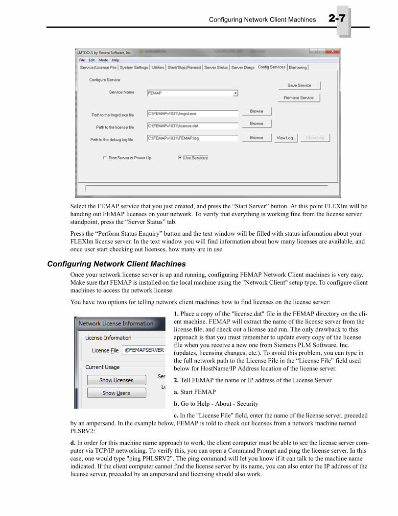
Security Device Not Found
Symptom:
You see an error indicating that the security device cannot be found.
Resolution:
Go to Section , "Security Device", and confirm all steps have been followed. Try to run FEMAP again.
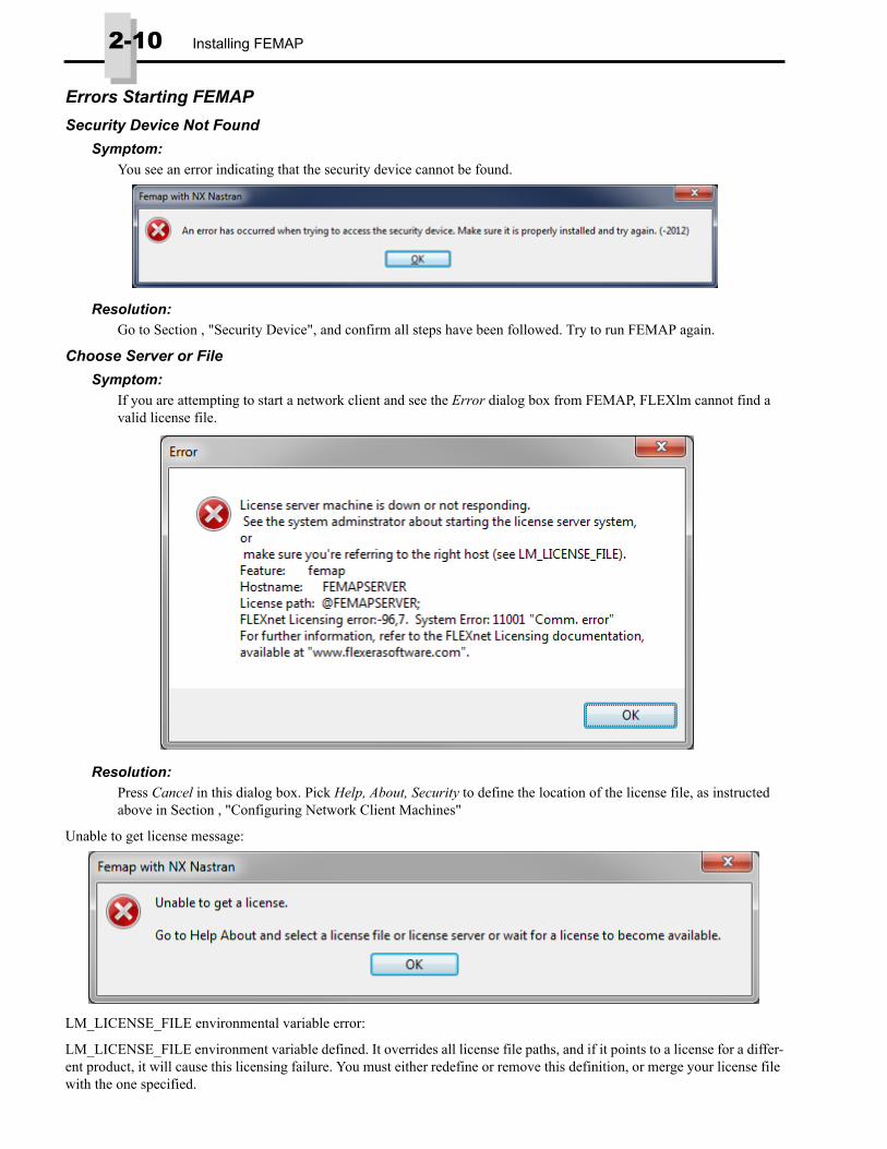
Choose Server or File
Symptom:
If you are attempting to start a network client and see the Error dialog box from FEMAP, FLEXlm cannot find a valid license file.
Resolution:
Press Cancel in this dialog box. Pick Help, About, Security to define the location of the license file, as instructed above in Section , "Configuring Network Client Machines"
Unable to get license message:
LM_LICENSE_FILE environmental variable error:
LM_LICENSE_FILE environment variable defined. It overrides all license file paths, and if it points to a license for a differ-ent product, it will cause this licensing failure. You must either redefine or remove this definition, or merge your license file with the one specified.

Improving Performance (RAM Management) 2-11
This error will ONLY occur when the environment variable LM_LICENSE_FILE has been set. For example, this environment variable may have been set by another application for licensing purposes. Be careful when removing or altering this environment variable as it may cause other applications to no longer function properly.
Other Error Messages
Symptom:
If you receive an “Unable to access {directory path}. Either this directory does not exist or you do not have proper permissions. Check the directory and your preferences” error or have any other difficulty starting FEMAP where abnormal termination occurs, you either do not have enough disk space, or your Windows TEMP is not set to a valid, accessible directory.
Resolution:
You may either change your Windows TEMP directory environment variable, or specify a path for the FEMAP scratch files (which default to the Windows TEMP directory set by the environment variable) to a valid directory.
This and all other FEMAP preferences are stored in a file called femap.ini that is typically located in the FEMAP executable directory. You will have to create this file or modify it to include the appropriate lines as shown below:
DISKMODELSCR=C:\FEMAP111
where C:\FEMAP111 can be any valid path. The DISKMODELSCR parameter is case sensitive and must be defined exactly as above. Once you make these changes and FEMAP starts, you can use the File, Preferences, Database command to modify this path.
Improving Performance (RAM Management)FEMAP determines the amount of available memory a machine and sets it to a default level automatically (20%).
FEMAP performance may improve on Windows personal workstations by modifying the default settings that FEMAP uses to manage RAM. To view or change these settings, use the File, Preferences command, then click the “Database” tab.
Database PerformanceThese options control how FEMAP uses your computer’s RAM. Setting these properly can greatly improve performance.
Database Memory LimitThe Database Memory Limit sets the maximum amount of system memory that FEMAP will use to hold parts of your model and results in memory. If your model is larger than the amount of memory that you choose, FEMAP will automatically read data from your disk as it is needed, replacing data that is not being used. While this “Swapping” process can slow down overall performance, it does let you work with much larger models than would otherwise fit into your available memory.
The Database Memory Limit DOES NOT control the total amount of memory that FEMAP will be using. FEMAP uses memory for many different operations – this is just one of them. Almost every command temporarily uses some small amount of additional memory. Some commands, like meshing, node merging and reading results can temporarily use fairly significant amounts of memory. Other operations, like loading large amounts of data into the Data Table require memory for a longer period of time – in this case as long as the data is in the table. Finally, the largest use of additional memory, and one which normally persists the entire time you have a model open is for drawing your model. For optimal performance, FEMAP uses OpenGL graphics, and keeps copies of the data to be drawn in memory at all times. You must always have suf-ficient free memory available for all of these uses, or the operations will not be able to execute properly. In the very worst case scenario, running out of memory could cause FEMAP to crash. It is for this reason that the default Database Memory Limit is set fairly low – 20% of the memory in your computer (The 32-bit version is also restricted by the 2 GByte limit for any program). This does not mean that you can not increase the limit beyond its default, but the further into the yellow and red zones you push the slider, you are increasing the chance of running out of memory.
Using the ControlThe slider control allows you to choose the amount of memory to use for the database. Move the slider to the left to reduce the limit, to the right to increase it. As you move the slider, the memory limit is updated and displayed above the slider.
Note: Changing the Database Memory Limit does not change the amount of memory used for the current session. For this selection to take effect, you must exit and restart FEMAP.

2-12 Installing FEMAP
The colored bar below the slider gives you an indication of the risk of run-ning out of memory if you use this setting. The yellow and red regions should be used with caution since there is a good chance of causing prob-lems with other operations like meshing and graphics. The small line along the top edge of the green section indicates the default memory limit. It is simply displayed to make it easy for you to go back to that limit if you try other settings. The blue bar along the bottom edge indicates the amount of
memory that the database is currently using.
With this option, you are simply setting the maximum amount of memory available for the database. If you are working with a smaller model, FEMAP will not use memory that it does not need and the blue bar will not extend the entire way to the slider setting. If you look at this control with an empty model, or if you have a small model and a large amount of memory in your system, the blue bar may not be visible – because it is too short to be seen along the bar.
Max Cached Label Sets the largest label that FEMAP will reserve memory for. This option must be set to a ID higher than any entity in the model. Default value is 5,000,000 for 32-bit FEMAP and 99,999,999 for 64-bit FEMAP.
Blocks/PageThis value sets the “page” size. The optimum setting of this number often depends on the speed of your disk and controller.
For more information, see Section 3.4.2, “Improving Performance (RAM Management)” in the FEMAP User Guide.
Licensing Conversion MethodsPlease read this section very carefully before changing your licensing method. If you are going to convert your licensing method you MUST HAVE FEMAP AND NX NASTRAN CLOSED (not running) before you use the files described below.
You can change your licensing method (i.e., from using a security key to using a network license) using specific “batch” files located in the FEMAP directory. The files are named “go_licensing method”.bat and require minimum user input to change your licensing method. In general, the “go” batch files change your current “auth_###.dll” to use the appropriate licensing method (auth_licensing method.dll) and may create or alter some other required files. FEMAP will open a “com-mand prompt” and let you know if the conversion of the auth_###.dll has been successful. The various “go” files are explained in greater detail below:
• go_apionly.bat - converts your current licensing method to the “API Only” version of FEMAP
• go_demo.bat - converts your current licensing method to the FEMAP Node-Limited Demonstration version.
• go_dongle.bat - converts your current licensing method to use a security key.
• go_network.bat - converts your current licensing method to use the FlexLM Network Client
Note: The blue bar in the above figure shows the amount of memory used by a 1,000,000 element model (4-noded plate elements) on a 32-bit machine with 2 GB of RAM. Most potential problems with exceeding the 2 GB memory limit only occur with very large models.
Note: The default value of “4” was determined via testing to produce the best performance over a wide range of values for Database Memory Limit and using the default settings for a number of different types of disk drives. You may want to try other values from 1 to 15 if you have changed any speed/caching settings on your drive or have “high-speed” drives to determine if performance is improved.

What’s New in FEMAP
FEMAP 11.1 includes enhancements and new features, which are detailed below:
User Interface
Model Merge
Geometry
Meshing
Elements
Materials
Properties
Loads and Constraints
Connections (Region, Properties, and Connectors)
Groups and Layers
Views
Output and Post-Processing
Geometry Interfaces
Analysis Program Interfaces
Tools
OLE/COM API
Preferences

11.1-2 Finite Element Modeling

What’s New for version 11.1 11.1-3
What’s New for version 11.1
User InterfaceGeneral, Menu, Toolbars, Model Info tree, Meshing Toolbox, PostProcessing Toolbox, Charting pane, Data Sur-face Editor, Data Table
General• Added “Performance Graphics” mode to improve performance of dynamic rotation and regeneration of large
models. Performance Graphics may be turned on in File, Preferences on the Graphics tab. See Preferences for more information.
• Added Layers/Groups in Tooltips option to include Layer and Group information in Tooltips and Rotate View About submenu to specify View Center options from the quick access menu (right-mouse click menu).
• Enhanced Modify, Renumber... commands which allow Coordinate renumbering to allow the user to specify the Order using the +/- X, Y, or Z locations of each entity.
• Enhanced the performance of Combo and List Boxes with lists of entities that have a large number of items. Also, enhanced performance of the Visibility dialog box. Previously, the dialog box could take longer than expected to appear when models had large numbers (50K-100K) of properties, materials, etc.
• Implemented Query and Front picking for Coordinate Systems. Only works for coordinate systems themselves, not selecting nodes or points referencing coordinate systems.
Menu• Added File, Merge command to File menu. See Model Merge (NEW for FEMAP 11.1!) for more information.
• Added Tools, Measure, Distance Between Geometry command to Tools menu. See Tools for more information.
• Added Geometry, Curve - Line, Between Geometry; Geometry, Solids, Sweep; and Geometry, Solids, Sweep Between commands to Geometry menu. See Geometryfor more information.
• Consolidated all “Point” commands in Modify, Project submenu into the Modify, Project, Point command and all “Node” commands in Modify, Project submenu into the Modify, Project, Node command. See Geometry for more information. Also, added Modify, Renumber, Load Definition and Modify, Renumber, Constraint Defini-tion command to Modify menu. Finally, added Modify, Update Elements, Rigid DOF command to Modify menu. See Elementsfor more information.
• Added List, Output, Contoured Results to Data Table command along with the List, Output, Freebody Nodal Summations and List, Output, Freebody Nodal Summations to Data Table commands to the List menu. See Out-put and Post-Processing for more information.
• Added Group, Operations, Generate Freebody Entities; Group, Curve, in Connection Region; Group, Surface, in Connection Region; Group, Node, in Connection Region; Group, Element, in Connection Region; and Group, Property, in Connection Region commands to the Group menu. See Groups and Layers for more information.
• Added Help, FEMAP User Community option to Help menu, which links to the official FEMAP Community website, hosted by Siemens PLM Software. Removed Help, Using Help command, as it no longer applied.
Toolbars• Added Distance Between Geometry icon to Measure icon menu of View Toolbar.
• Added Layers/Groups in Tooltips icon to Selector Mode icon menu of Select Toolbar.
• Added Renumber command to context-sensitive menus for Solids, Connection Properties, Regions, Connec-tors, Coordinate Systems, Materials, Properties, and Layups. In all cases, a dialog box appears requesting ID and selected entities will be renumbered using the Original ID method of the Modify, Renumber... commands.

11.1-4 Finite Element Modeling
• Updated “Next Output Vector” and “Previous Output Vector” icons on the Post Toolbar to increment all 3 pos-sible contour vectors if they are defined. Previously only the primary vector was incremented.
Model Info tree• Added ability to toggle on/off the current count of various entity types using the Show Entity Counts icon in the
Model Info toolbar.
• Added ability to “scroll” through entities using the middle mouse button while the cursor is over the Entity Icons or Visibility check boxes now available while in another command, except View commands.
• Added Renumber command to context-sensitive menus for Coordinate Systems, Geometry, Connection Proper-ties, Regions, Connectors, Aero Panels/Bodies, Aero Properties, Aero Splines, Aero Control Surfaces, Materi-als, Properties, Layups, Load Sets, Load Definitions, Constraint Sets, Constraint Sets, Functions, Analysis Sets, Output Sets, Groups, and Layers. In all cases, a dialog box will appear starting ID and the selected entities will be renumbered using the Original ID method of the Modify, Renumber... commands.
• Added Attach to Results command to context-sensitive menu for Results, which displays the Manage Results Files dialog box from the File, Attach to Results command.
Meshing Toolbox• Locator tool - Added “With Poles” option when Search For is set to Surfaces. When on, the Locator will find
any surface which contains a “pole”. Typically only spherical or conical surfaces and planar surfaces of revolu-tion around a point can have a “pole”.
• Geometry Editing tool - Added “Split at Closest” option to the “Edge to Edge” Operation. When on, will attempt to create the shortest possible curve using the two locations on the selected curves closest to one another. Also, added Pad Alignment and Add Washer options to the “Pad” Operation.
PostProcessing ToolboxIn the Contour Tool:
• Added No Average, Centroid Only option for Data Conversion in the Options section when Style is set to Con-tour. Simply allows all possibilities currently available through the menus and dialog boxes.
In the Freebody Tool:
• Added ability to display freebody results in nodal output coordinate system. Only nodal vectors and quantities will be displayed in the nodal output coordinate system. Interface loads will still be in the freebody coordinate system.
• Added Allow Alternate Vector option in the Freebody Contributions section for the Applied, Reaction, and Mul-tiPoint Reaction contributions. When on, attempts to use alternate vectors if the Grid Point Force Balance vec-tors are not available for a particular contribution.
• Added option to List Nodal Sums when using the listing commands in the Freebody Tools section. When used, summed values for Fx, Fy, Fz, Mx, My, and Mz at each node will be added to the listing using **SUM** as the Source.
• Added Freebody Validation icon to Freebody Tools section. Model debugging tool that can be used to help determine if results requested for a given freebody exist in the database for the selected set of elements and/or nodes. It does not indicate that the results of a freebody calculation are a valid idealization of the structure being analyzed, as that is up to the individual user to determine.
Charting pane• Reorganized the Chart Data Series dialog box into a tabbed format and added the Vector vs. Vector option as a
tab. See Tools for more information.
• Added ability to set the Font Size for the Legend, Chart Axis Labels, and Labels in the Chart.
• Changed Show Tooltips icon into icon menu and added several options for syncing up the active graphics win-dow to the data point currently showing the Tooltip and ability to control what is shown in the Tooltip. See Tools for more information.

Data Surface Editor 11.1-5
• Changed Copy Chart to Clipboard icon into icon menu offering three options, Copy Chart Image, Copy Chart Data, or Copy Chart Image and Data. The most recently used option will remain the default option for the cur-rent instance of FEMAP.
• Moved the Title field from the Chart Title tab to the top of the in the Charting dialog box.
• Added List Data command to Data Series context-sensitive menu to list the data from the Data Series to the Messages window
• Added Show (Element/Node ID) in Active View command to Marker context-sensitive menu to highlight the entity in the active view using the current Show When Selected options, except always displays label.
Data Surface Editor• Added Load Set Combination Data Surface to Create/Load Data Surface icon menu. See Loads and Con-
straints for more information.
Data Table• Added Significant Digits options to Show/Hide Columns icon menu. Simply allows you to specify the number
of significant digits to be displayed for values in the Data Table. The number of significant figures will persist until the Data Table is closed.
• Added Sum Selected Rows command to context-sensitive menu for column headers. Displays a dialog box with the Minimum Value, Maximum Value, and Sum using data from the rows currently highlighted.
Model MergeNEW for FEMAP 11.1! The File, Merge command allows entities from any model currently open in the same instance of FEMAP to be “merged” with the active model. At least two models must be open for this command to be available. To facilitate bringing entities into the active model, a number of overall Renumbering and Duplicates Strategy, Entity Selection, and Model Orientation options are available in the Model Merge Manager dialog box and will be described in detail later in this section. In addition, the top portion of the dialog box, the Entities to Merge list can be used to choose which entity types to merge into the active model using the check marks in the Entity Type column.

11.1-6 Finite Element Modeling
If more than two models are open in the same instance of FEMAP, use the From Model drop-down to select the desired open model. The Entities to Merge list will update whenever a different model is selected using the From Model drop-down. The To Model field is always gray and simply displays the name of the active model.
Entities to Merge list
Contains a list of the entities to merge into the active model with columns for Entity Type, Current IDs, Merge IDs, Renumber To, and Renumbering. Use the All On or All Off buttons to check/uncheck all of the Entity Type check boxes for all entities in the list.
Once the Entities to Merge list is filled, the row(s) must be highlighted for any of the options in the Renumbering and Duplicates Strategy and/or Entity Selection sections to take effect. Multiple rows may be selected for update (Hold the CTRL key when you click to choose multiple entity types one at a time or the SHIFT key to choose a range of entity types). The Select All and Select None buttons are used to select/de-select all of the different entity types in the list. Once the desired rows are selected, choose the appropriate options and then click the Update Selected button and review the updated information in the columns. Alternatively, use the Update All button to update all entity types with the current settings for the various options.
• Entity Type - column simply contains the name of the entity type and a check box which allows you to include or not include that entity type when merging.
• Current IDs - column lists the IDs for each entity type in the active model. If the active model does not have any entities of a certain entity type, then this column will be blank.
• Merge IDs - column lists the IDs found in the model selected using the From Model drop-down. The options in the Entity Selection section are helpful when trying to limit the IDs in this column.
• Renumber To - column lists the “new” IDs for the entities found in the Merge IDs column. These IDs are based on the settings in the Renumbering and Duplicates Strategy section.
• Renumbering - column lists the number of entities which will be renumbered. When they occur, this column will also list the number of “Conflicts” and “Overwrites” which will occur using the current settings in the Renumbering and Duplicates Strategy section.
Renumbering and Duplicates Strategy
This sections is used to specify how entities will be renumbered and how to handle duplicates.
• None - specifies that entities should not be renumbered. This option can only be used effectively when the Overwrite Duplicates option is also selected.
• Minimal Renumbering - specifies that renumbering should occur using the lowest IDs possible. If unused IDs exist within the range of Current IDs, this renumbering strategy will use those IDs. This is the default setting. Optionally, you can enter a value into the Renumber To field to specify a different starting ID. If the stating ID is not available, the next available ID will be used instead. For instance, if there are 20 elements in the active model and the elements are numbered 1-10 and 31-40, Minimal Renumbering would place the 30 elements found in the From Model into element IDs 11-30 (20 elements with the lowest IDs in the From Model) and 41-50 (remaining elements in the From Model).
• Block Renumbering - specifies that renumbering should be done using a block of IDs, based on the largest value for Current IDs. Optionally, you can enter a value into the Renumber To field to specify a different start-ing ID, but if the specified value is in the range of Current IDs, it will be updated to the lowest available ID out-side the range. For instance, if there are 20 elements in the active model and the elements are numbered 1-10 and 31-40, the block of Current IDs would be from 1 to 40. Block Renumbering would place the 30 elements found in the From Model into element IDs 41-70, leaving element IDs 11-30 empty.
• Offset Renumbering - specifies that renumbering should be done using the original Merge IDs plus a value specified using the Offset By field. For instance, if there are 20 elements in the From Model and the elements are numbered 1-10 and 31-40, using Offset Renumbering and entering an Offset By value of 100 would renum-ber these elements to 101-110 and 131-140.
• Compress - specifies the Merge IDs should be compressed in an attempt to remove any gaps in the ID range of the From Model. Optionally, you can enter a value into the Renumber To field to specify a different starting ID. If the stating ID is not available, the next available ID will be used instead. For instance, if there are no elements in the active model and the elements in the From Model are numbered 1-10 and 31-40, Compress would renum-ber the 20 elements found in the From Model into element IDs 1-20.

Model Merge 11.1-7
• Renumber Duplicates - when this option is selected, any duplicate entity IDs will be renumbered to available IDs based on the selected renumbering option.
• Overwrite Duplicates - when this option is selected, any entity ID in the active model which is also found in the From Model will be overwritten by the entity in the From Model.
Entity Selection
This section is used to limit the entities which appear in the Merge IDs column for each entity type. The Merge IDs are then used to populate the Renumber To and Renumbering columns based on the options set in the Renumbering and Duplicates Strategy section. In all cases, the desired rows should be selected before setting this option and clicking wither Update Selected or Update All.
• None - specifies that no entities should be in the Merge IDs column. This option is really only used to clear col-umns in the selected rows.
• All In Model - specifies that all entities in the model should be used to populate the Merge IDs column. This is the default.
• From Group - specifies that only entities in the selected group should be used to populate the Merge IDs col-umn. If an no entities of a specified entity type are in the group, the Merge IDs column for that entity type will be empty.
• ID Range - specifies an ID range to use for all entity types (rows) currently selected in the Entities to Merge list. For instance, if Node and Element are selected in the Entities to Merge list and an range is entered From 1 To 100, then the Merge IDs column for both nodes and elements would show 1..100 (or 1..highest existing ID under 100).
• Select - allows selection of Merge IDs for a single entity type using the standard entity selection dialog box. If multiple entity types are highlighted in the Entities to Merge list, only the entity type closest to the top of the list will be updated.
• Add Referenced Entities button - adds entities referenced by other entity types currently in the Entities to Merge list. For instance, if Entity Selection is set to Group and the selected group only contains elements which have been sent to the Entities to Merge list, then pressing this button will add Node, Material, Property, and Layer entity types, and potentially some others, to the Entities to Merge list.
Model Orientation
This section is used to orient the From Model in the active model. In addition, options in the section control behav-ior of transferred groups, optionally create of a new group in the active model, optionally create parent coordinate systems for the merged model, and optionally limit certain entity types.
• Create Group for Merged Model - when on, creates a group containing all of the entities merged from the From Model into the active model.
• Create Parent CSys for Merged Model - when on, creates a “parent” Coordinate Systems in the active model for the entities found in the From Model. The number of “parent” coordinate systems created varies from one to three and depends on how many of the Basic Coordinate systems are using in the From Model. When only the Basic Rectangular coordinate system is referenced by entities, a single rectangular coordinate system located at the origin (0, 0, 0) will be created. If the Basic Cylindrical and/or Basic Spherical coordinate system is refer-enced by entities, then a single rectangular coordinate system located at the origin will be created along with a cylindrical and/or spherical coordinate system referencing the newly created rectangular coordinate system.
• Condense Transferred Groups - when on, any groups brought into the active model from the From Model will be “condensed”. See "Group, Operations, Condense..." in Section 6.4.3.2, "Group, Operations Menu" for more information.
• Limit Loads, Constraints and Contact to Merged Entities - when on, will only transfer loads, boundary condi-tions, and connection entities from the From Model when the entities referenced by these entity types are also being merged into the active model. For instance, if a load set contains nodal loads on node 1 and node 10, but only node 1 is being brought into the active model, then only the load on node 1 will be transferred to the active model.
Note: Great care must be taken when using the Overwrite Duplicates option. For instance, importing an ele-ment with the same ID, but of a different type could create a model which is invalid.

11.1-8 Finite Element Modeling
• Transform Merged Model - when on, the entities from the From Model will be transformed using the From coordinate system found in the From Model to the To coordinate system found in the active model.
Duplicates to the Data Table button - only available when the Data Table is open. When pressed, sends a listing of duplicate entities currently found in the Entities to Merge list to the Data Table. Each duplicate entity is listed in a single row with Entity Type, Entity ID, and Renumber To columns.
Geometry• Updated Geometry, Midsurface, Automatic command to use Parasolid “face pairing” technology.
Attempts to use face pairing technology in the Parasolid modeling engine to automatically create a midsurface rep-resentation of a solid part or between selected surfaces. The command requires you to select the surfaces, specify a Target Thickness (midsurface tolerance), and optionally set some additional settings
You may want to click the Distance icon button to use the measuring tool to specify an effective Target Thickness. Any surfaces with a distance between them less than the Target Thickness will have a midsurface generated.
When on, the pre-V11.1 Midsurface Method runs the three steps of semi-automatic midsurfacing (Generate, Inter-sect, and Cleanup below) at once instead of using the more advanced face pairing technique. Also, when using pre-V11.1 Midsurface Method, none of the other options are available.
When on, Combine Midsurfaces simply performs a Geometry, Surface, NonManifold Add on the newly created sur-faces in an attempt to create a general body, which usually aids when trying to create a mesh.
The Face Pairing Options can be used in an attempt to create a more accurate midsurface representation:
Combine Tangent Surfaces - collects all connected tangent faces, based on the Angle Tolerance specified, finds all faces opposite these faces, then creates a larger face pair set. By doing so, sheet metal parts and similar will mid-surface faster and more accurately with the additional connection information implied by the larger face pairing.
Reverse Face Pairs - simply reverses the two opposite faces or sets of faces in the face pairing algorithm. Turning on this option sometimes helps in achieving a better midsurface on complicated parts with a high level of curvature. If you are not satisfied with midsurface results, this option may help.
Note: The Limit Loads, Constraints and Contact to Merged Entities option should only be turned off when merging a model which is very similar or identical to the active model. Otherwise, loads, constraints, and/or contact entities may be applied to random entities in the active model.
Note: When using Transform Merged Model, the Output Set entity type must NOT be selected. If it is, the com-mand will issue a message stating “Unable to transfer results when transforming a model during merge.”
Note: The resulting midsurface created by the Parasolid face pairing algorithm will always be an constant off-set from one face or the other. In some cases, this will require the user to do some additional modifica-tion of the geometry or mesh to account for non-constant offset regions in the model.

Geometry 11.1-9
• Added Geometry, Curve - Line, Between Geometry command
Creates a three-dimensional line by using the minimum or maximum distance (or both) between two sets of selected geometric entities. For more information, see "Tools, Measure, Distance Between Geometry...".
In the Distance to Find section, choose from Minimum, Maximum, or Both to select distance to use when creating the line(s).
Select an entity type in the From section of the dialog box from Point, Curve, Surface, or Solid, then select the same entity type or a different entity type in the To section. Geometric entities for From and To will be selected using the standard entity selection dialog box later in the command.
The Overall Only option found in both sections is on by default. When “on” in both the From and To sections, the command will only create a line between the two geometric entities used to calculate the Minimum and/or Maxi-mum distance. If Overall Only is “off” in both sections, then lines will be created between ALL geometric entities in the From section to ALL geometric entities in the To section, based on the Distance to Find setting. If Overall Only is only “on” in one of the sections, then lines will be created between ALL of the geometric entities selected in the section where the option is “off” to the appropriate geometric entity where the option is “on”.
• Upgraded Geometry, Surface, NonManifold Add command to use new “tolerant modeling” capabilities avail-able to create “General Bodies” when using the Parasolid Geometry modeling kernel.
The Tolerance value now works much like a “stitching tolerance” and can now make slight alterations to the geom-etry in order to bring geometry together in “general bodies”. For instance:
Also, the new Incremental Checking option will check the body is valid after each sheet solid or solid is added to the “general body”. If adding a sheet solid or solid causes the “general body” to become invalid, the command will revert one step to before the particular sheet solid or solid was added, then skip it and try to add the next one.
• Added Geometry, Solid, Sweep command.
Allows creation of solids by moving or sweeping one or more boundary surfaces and/or surfaces along a continu-ous path defined by any number of curve. The required input for this command is minimal. You simply select the boundary surface(s) and/or surface(s) that define the cross section(s) that you want to sweep, using the standard entity selection dialog box. Then with a second entity selection dialog box, you select the curves that make up the continuous path along which you will sweep the cross section.
Before NonManifold Add After NonManifold Add

11.1-10 Finite Element Modeling
Selecting the Path
Even though you choose it after the surface(s) to sweep, it is important to understand the implications of choosing a path before you select the surface(s). The curves that you select for the path must form a single continuous loop - either closed (the end is also connected to the start) or open. They must not branch, or have any gaps. They do not have to be connected to the same points, but must have coincident end points.
If, in addition to being coincident, all curves along the path are also tangent at their end points, the sweeping oper-ation will maintain a constant cross section as it traverses the path. On the other hand, if you include non-tangent curves, the corners will be automatically mitered to the half angle between the tangents of the curves. This, how-ever, will result in a nonuniform cross section, and in some cases a cross section that is somewhat distorted.
Choosing Splines in the Path
You can use any type of curves in the path; however, if you are using the standard FEMAP geometry engine, this command cannot create a single swept surface along a spline. If you choose splines in the path, they will be broken into multiple line segments, and the cross section will be swept along these segments rather than the true spline. This will result in multiple surfaces. You can control the number of line segments by setting the mesh size along the spline prior to sweeping using the Mesh, Mesh Control, Size Along Curve command.
Selecting the Cross Section
Just as for the path, you can choose any curves that you want for the cross section. You do have to be aware, how-ever, of the relationship between the path and the cross section.
Here are some general rules to follow:
1. The boundary surface(s) and/or surface(s) must be positioned in space at the appropriate location relative to the path. This command simply extrudes and revolves the cross section along vectors which are defined by the curves you select as the path. It is up to you to properly locate the starting position of the cross section. The sol-ids created by this command will be located wherever you start the cross section. All offsets from the path to the cross section will act as rigid links as the cross section is swept around a curve.
2. If your path contains arcs, make sure that your cross section does not protrude further than the arc radius to the “inside” of the path. If it does, the resulting solid(s) will be twisted as they are swept around the arc.
3. Typically you will want to create the cross section surface in a plane that is normal to the ending tangent of the path. If you do not, the cross section that you sweep will be a projection of the true cross section
4. If the cross section that you choose contains arcs or circles, and your path contains curves that are not tangent to one another, the arcs and circles will be converted to equivalent splines before they are swept. This is not a pre-cise representation, but it is fairly accurate. It is required because of the automatic mitered corners that will be generated between the non-tangent curves. The cross section at those corners will no longer be circular, it will be elliptical (which must be represented by a spline)
• Added Geometry, Solid, Sweep Between command.
Cross Section Surface
Path Curves
Front View - Before Isometric View - Before Front View - After Isometric View - After
Mitered corner wherepath was not tangent
Path Curves

Geometry 11.1-11
Allows creation of a solid between two selected surfaces. A single point on each surface is also selected and used as a reference. The selected points are used by the command to determine which curves on each surface should be “matched”. The Sweep Type (“path”) used to create the solid may be Linear or Splined.
The number of curves on the two selected surfaces do not need to match, but a similar number of curves tends to create a solid with a more predictable shape.
When Sweep Type is set to Linear, ruled surfaces are simply created from each curve on the From surface to a “matching” curve on the To surface (From and To points shown as black squares):.
When Sweep Type is set to Splined, a Blend Factor may also be used to control the shape of the solid. By specifying number larger than 1.0, the solid will closely follow the tangents of the normal vector at the centroid of each sur-face for a larger distance, typically causing more curvature near the center of the solid. Smaller numbers make the tangency weaker, therefore, most of the curvature will be near the original surfaces. The figure shows some possi-bilities (From and To points shown as black squares)
• Added Add Washer option to Geometry, Curve - From Surface, Pad command.
Note: A solid cannot be created between surfaces if either selected surface has any interior loops.
Original Solids From Surface To Surface New Solid
Original Solids From and To Blend Factor = 1.0Surfaces
Blend Factor = 1.25 Blend Factor = 0.75

11.1-12 Finite Element Modeling
When the Add Washer option is selected, the same overall sizing of the “pad” will be used, but a “washer” will be added around the hole and extend to half the distance of the overall “pad”.
• Updated Mesh Sizes, Loads, Constraints... option in various Geometry, Copy/Scale/Rotate/Reflect commands to now also include regions of all types.
• Replaced Modify, Project commands for points with single Modify, Project, Point command.
This command updates the locations of points by moving them onto a selected curve or surface or onto a specified vector or plane. When you project points, any entities that reference those points may also be moved.
The following dialog box is used when projecting points:
There are two sections in the dialog box, Project Onto and Direction. The Project Onto section allows the user to select the destination of the projected points. The Project Onto destination options may be any number of selected Surface(s) or Curve(s), a single Vector, or a single Plane.
The Direction section controls the approach used to project the points onto the destination.
• Closest/Normal - generally uses a vector normal to the curve, surface, vector, or plane that is selected as the destination. Actually, this moves the points to the ‘closest’ location on the curve, surface, vector, or plane.
• Along Vector - allows the user to select a vector to ‘project along’. This option will almost always result in the points actually being located on the destination entity, even if a secondary projection is required. One excep-tion, if the projected vector from a point location does not intersect the selected surface(s), then nothing will happen.
Project Onto - Surface(s)
Moves one or more points onto any number of selected surfaces.
The standard entity selection dialog box is used to choose the points to project. Then, simply select the surface(s). You can choose any number of surfaces, and the selected points will be projected onto them based on proximity and specified Direction.
When Direction is set to Along Vector, the Both Directions option is available. When “on”, the points will be pro-jected in both the positive and negative direction of the specified vector. This allows you to attempt to project points which lie above and below a surface using a single command.
Original Surface Normal Pad Pad with Add Washer

Geometry 11.1-13
For Example:
Project Onto - Curve(s)
Moves one or more points onto any number of selected curves.
The standard entity selection dialog box is used to choose the points to project. You then must select the curve(s). You can choose any number of curve(s) and the selected points will be projected onto them based on proximity and specified Direction.
When Direction is set to Closest/Normal, the Extend Curves option is available. When “on”, the curves extend past their endpoints toward infinity, or in the case of an arc, they extend a full 360 degrees. When “off”, the points will be projected using the extents of the actual curve, which many times results in the projected points being located on the end point(s).
For example:
Project Onto - Plane
Moves one or more points onto a single 2-D plane specified by the user.
The standard entity selection dialog box is used to choose the points to project. You then must specify the plane using the Plane Locate dialog box and the points will be projected onto it based on proximity and specified Direc-tion. If Direction is set to Along Vector, the vector is specified before the plane.
Project Onto - Vector
Moves one or more points onto a single vector specified by the user.
The standard entity selection dialog box is used to choose the points to project. You then must specify the vector using the Vector Locate dialog box and the points will be projected onto it based on proximity and specified Direc-tion. If Direction is set to Along Vector, the vector to ‘project along’ is specified before the ‘project onto’ vector.
Projected Points
Original Points
Surface
Original Locations Projected Locations
Points projected onto“extended” curve
Point projected onto“extended” arc
OriginalProjected LocationsLocations

11.1-14 Finite Element Modeling
Meshing• Added several new options to the Mesh, Geometry, Solids command to improve tetrahedral meshing.
In the Automesh Solids dialog box:
Multiple Tet thru Thickness
When on, the tet-mesher will attempt to place at least 2 elements through the thickness throughout the model. This will not split any elements on the outer surfaces, so if you need at least 2 elements through the thickness every-where, try and size the solid so the surface mesh has at least 2 elements from one side of each surface to the other.
Tet Sliver Removal
When on, which is the default, attempts to remove tetrahedral elements considered ‘slivers’ near the boundary. A sliver is defined as a tetrahedral when at least one angle less than 5 degrees. In most cases this will improve mesh quality and should only be turned off if there is a problem.
Tet Optimization
Sets an optimization level (mesh quality vs. speed) for the tetrahedral mesher. Using a higher value does not guar-antee improved mesh quality. “3..Default” is the best compromise between speed and quality, while choosing “0..None” will simply not use do any optimization. Setting to “1..Minimal” will potentially create a lower quality mesh in less time, while “5..Maximum” will potentially create a higher quality mesh, but take longer.
In the Solid Automeshing Options dialog box:
Quadratic Mesher/Jacobian Correction
When this option is on, the tetrahedral mesher will add the midside nodes during the meshing operation instead of midside nodes being added after the tetrahedral mesher has created 4-noded tetrahedral elements. The Jacobian Correction option is only available when using the Quadratic Mesher and, when on, will attempt to create elements with the best possible Jacobian element quality.
Desired Edge Length - Min and Max
Allows you to enter values for minimum (Min) and maximum (Max) desired edge length. Based on geometry, these values may not be attainable, but the tetrahedral mesher will attempt to use them as a guideline.
Pre-v11.1 Tet Meshing
The tetrahedral meshing in FEMAP has dramatically changed for version 11.1. This switch allows you to use the “pre-v11.1” tetrahedral meshing if you feel more comfortable with this mesher and associated default values.
• Added Copy Method section to Mesh, Copy, Element command, with the default Copy Method being Along Vector which was previously the only option. The Normals and Normals with Thickness Correction options were added for planar elements only and work in the same manner as when extruding or offsetting elements.
• Added Along Vector to Surfaces option to Mesh, Extrude, Curve; Mesh, Extrude, Element; and Mesh, Extrude Element Face commands.

Elements 11.1-15
For the Along Vector to Surface method, you will be asked to specify the extrusion vector using the standard vector dialog boxes. The vector can be located anywhere but must have the direction that you want for the extrusion. You will also be prompted to select any number of surfaces to project the curves onto along the specified vector.
For the Along Vector to Surface method, you will be asked to specify the extrusion vector using the standard vector dialog boxes. The vector can be located anywhere but must have the direction that you want for the extrusion. You will also be prompted to select any number of surfaces to project the elements onto along the specified vector.
• Replaced Modify, Project commands for nodes with single Modify, Project, Node command. Has all the same options as the Modify, Project, Point command, described in the Geometry section.
Elements• Added Pyramid as an Element Shape for Solid Element Type.
May only be created manually using the Model, Element command or imported in from an analysis input file.
Extrusion
Mesh Sizealong curves
Original Curves Extruded Elements
Surface
Vector
Extrusion vector
Extrude as Solids
Original Line Elements
Extrude as Plates
8 elementsalong length
8 elementsalong length
Original Plate Elements

11.1-16 Finite Element Modeling
Both the 5-noded linear pyramid and 13-noded parabolic pyramid are supported.
Linear and Parabolic Pyramid elements are only supported for NX Nastran and MSC Nastran.
• Added Modify, Update Elements, Rigid DOF Command
Allows you to change the Dependent and/or Independent degrees-of-freedom for existing rigid elements in your model. First select the Rigid elements to update, then the Update Rigid Degrees of Freedom dialog box will appear to select DOF.
The dialog box has two sections, one for the Dependent DOFs and one for the Independent DOFs. Both sections contain an Update DOF check box, which must be on for those DOFs to be updated, and check boxes representing the 6 DOFs available for update. When modifying RBE2 elements, only the Update DOF option in the Dependent section will be used, while both sections will be available for RBE1 and RBE3 elements.
• Added Along/Between Path option to Modify, Update Elements, Material Orientation command.
The Along/Between Path(s) option can be used to align the orientation angle to any number of selected curves based on the specified Project Method, which controls how the centroid of each element is projected onto each curve. Essentially, the center of the element is projected to the path, then the tangent to the path at that location is used as the orientation vector. When Project Method is set to “0..To Closest Location on Path”, the normal vector is determined by projecting the center of each element onto the curves. When Project Method is set to “1..Specified Direction” the supplied vector is used as the normal vector. Entering a value for Angle From Path simply rotates the determined orientation vector around the element normal by the specified angle value.
Materials• Added 606..MSC.Nastran Fluid Material (MAT10) to Other Types.
Properties• Added Nastran Elbow/Pipe Options section to Curved Tube property.
Note: If a mixture of RBE2 and RBE1/RBE3 elements are selected, then the selected element with the lowest ID will be used to set the default state of the dialog box.Any non-rigid element is simply skipped.

Loads and Constraints 11.1-17
There are Nastran specific options in the NASTRAN Elbow/Pipe Options section, which, when used, will write additional fields using alternate form of the PBEND entry for “Elbows ans Curved Pipes”.
When the Flexibility/Stress Intensification, FSI is set to “1..Default”, only the Internal Pressure, Radial Offset, and Perpendicular Offset additional fields may be specified. Selecting any other option and entering the available val-ues will populate other additional fields on the PBEND entry. Please consult the documentation for your version of Nastran to determine which FSI options are available as well as review information on specifying appropriate val-ues.
Loads and Constraints• Enhanced Load creation to allow the use of Data Surfaces when defining loads of the following types: Force on
Curve, Force Per Length on Curve, Moment on Curve, Moment Per Length on Curve, Force on Surface, Force Per Area on Surface, Moment on Surface, Moment Per Area on Surface, Nodal Heat Flux on Curve, Nodal Heat Flux Per Length on Curve, Nodal Heat Flux on Surface and Nodal Heat Flux Per Area on Surface. For the load types that support it, this capability also works with or without the “Total Load” option.
• Updated load expansion from geometry to a mesh for elemental face-based loads on surfaces (Pressure, Heat Flux, Convection and Radiation). Previously on large models these could an extended period of time.
• Updated Model, Load, Combine command to allow a number of new options.
Now enables you to create multiple load set combinations. Each load set combination will be used to create a new Standard load set or a new Nastran LOAD Combination load set based upon the following formula
Load A1Load1 A2Load2 AnLoadn+ + +=

11.1-18 Finite Element Modeling
The Combine Load Sets dialog box has five sections, Combine To, Set Type, Options, the From list, and the Load Set Combinations list, each of which is described in detail later in this section:
Temperature loads will not be linearly combined. FEMAP will simply copy the nodal and elemental temperatures. If conflicting temperatures exist for the same node or element in the individual load sets, FEMAP will use the last temperature. Also, If loads exist on the same node or element in different sets that are combined, the resulting set will simply obtain multiple loads on that node or element, which can then be combined with Tools, Check, Coinci-dent Loads.
Combine To
This section is used to select how many scale factors can be entered for each load set in the From list, along with controlling how the Load Set Combinations list is populated and which Options are available.
• Single Load Set - only a single scale factor may be set for each load set in the From section. Also, a single load set may be sent to the Load Set Combinations list and you can choose to send the load to an existing load set, but you can also choose to create a new load set, which is the default.
• Multiple Load Sets - any number of different scale factors may be set for each load set in the From section. Also, at least two load sets must be highlighted in the From section to allow them to be sent to the Load Set Combinations list. The Auto Zero Factors and Single Set Combinations options also become available and new load sets will always be created.
• From Data Surface - the only item available will be the Data Surface drop-down, which is used to select a “Load Set Combinations Data Surface”. New load sets will always be created.
Set Type
This section allows you to select the type of load sets that should be created by the command. All new load sets cre-ated during one use of the command will be the same Set Type. Choosing Standard will create a normal load set, while selecting Nastran LOAD Combination will create a load set which creates a LOAD entry when exported to a Nastran solver. See “Creating New Load Sets” in Section 4.3.1.1, “Model, Load, Create/Manage Set...” for more information on the different types of load sets.
Note: The Multiple Load Sets option should only be used when multiple scale factors need to be set for a single load set. Otherwise, simply use the Single Load Set option.

Loads and Constraints 11.1-19
Options
Depending on the Combine To option selected, different options in this section will be available.
To Set - only available when Combine To is set to Single Load Set, Set Type is set to Standard, and there is a single entry in the Load Set Combinations list. Allows you to add a single load combination to an existing load set instead of creating a new load set, which is the default.
Title - allows you to enter a title which will be used for all new load sets created by a single use of the command.
Data Surface - only available when Combine To is set to From Data Surface. Allows selection of a “Load Set Combination Data Surface” via a drop-down. See "Load Set Combination Data Surface" in Section 7.2.6.1, "Data Surface Definition Methods" for more information.
Auto Zero Factors - only available when Combine To is set to Multiple Load Sets. When on, adds a “0.0” scale fac-tor to each load set which has at least one scale factor specified, which creates additional load sets.
For example, if Load Set A has 2 scale factors specified and Load Sets B and C have a single scale factor specified, and this option is on, the following combinations would be created:
Scale Factor 1*A + Scale Factor*B + Scale Factor*C
Scale Factor 2*A + Scale Factor*B + Scale Factor*C
0*A + Scale Factor*B + Scale Factor*C = Scale Factor*B + Scale Factor*C
Scale Factor 1*A + 0*B + Scale Factor*C = Scale Factor 1*A + Scale Factor*C
Scale Factor 1*A + Scale Factor*B + 0*C = Scale Factor 1*A + Scale Factor*B
Scale Factor 2*A + 0*B + Scale Factor*C = Scale Factor 2*A + Scale Factor*C
Scale Factor 2*A + Scale Factor*B + 0*C = Scale Factor 2*A + Scale Factor*B
If this option is off, only the following combinations would be created:
Scale Factor 1*A + Scale Factor*B + Scale Factor*C
Scale Factor 2*A + Scale Factor*B + Scale Factor*C
Single Set Combinations - only available when Combine To is set to Multiple Load Sets. When on, adds an item to the Load Set Combinations list containing only a single load set with a scale factor for each load set selected in the From list, along with adding all of the other combinations. If more than one scale factor is set for a particular load set, each scale factor times the load set will become an individual entry in the Load Set Combinations list.
From list
When Combined To is set to Single Load Set:
Choose any number of load sets from the From list (Hold the CTRL key when you click to choose multiple load sets one at a time or the SHIFT key to choose a range of load sets), then enter a Scale Factor (Default is “1.0”), then click Add Factors. If a load set already has a scale factor specified, clicking Add Factors will overwrite the scale factor for each highlighted load set. Once you have a single scale factor entered for each desired load set in the From list, you can use the Add Combinations button to add the combination to the Load Set Combinations list.
When Combined To is set to Multiple Load Sets:
Choose any number of load sets from the From list, then enter a Scale Factor, then click Add Factors. If a load set already has a scale factor specified, clicking Add Factors will add an additional scale factor for each highlighted load set. You can also use the “...” button to enter up to 10 scale factors at once for the highlighted load sets using the Combine Load Set Factors dialog box (use Clear Multi Factors button to clear the Combine Load Set Factors dialog box). Once you have the desired number of scale factors entered for each desired load set in the From list, use the Add Combinations button to add the combination to the Load Set Combinations list. Multiple combinations will almost certainly be added to the list and depending on the specified Options, the number of new load sets can vary quite a bit.
The Remove Factors button will remove the entered scale factor(s) for each load set currently highlighted in the From section, while Remove All Factors will clear all scale factors currently in the From section.

11.1-20 Finite Element Modeling
Load Set Combinations list
This section contains a list of all the load set combinations to create after clicking OK in the Combine Load Sets dialog box. Each item in the list represents a different load set to create. If only one item is in the list, Combine To is set to Single Load Set, Set Type is set to Standard, and To Set is set to an existing load set, then that load set will be updated instead of a new load set being created.
The Remove Combinations button will remove the combinations currently highlighted in the Load Set Combina-tions list (Hold the CTRL key when you click to choose multiple load set combinations one at a time or the SHIFT key to choose a range of load set combinations), while the Remove All Combinations button will remove all the combinations from the list.
• Added Load Set Combination Data Surface to Data Surface Editor.
This Data Surface has one very specific use, to cre-ate new load sets based on existing load sets. Each selected existing load set will appear in the Data Surface Editor as an indi-vidual column, while each new load set to create will appear as a row.
Use the Set Type to Create option to choose the type of load set(s) to create,
Standard or Nastran LOAD Combination load sets. See Section 4.3.1, "Create/Activate Load Set" for more infor-mation on Load Set Type. Combinations of existing Nastran LOAD Combinations load sets can be created by using the referenced load sets of each Nastran LOAD Combination at the time of creation in the new Nastran LOAD Combination load set.
In the Options section, turn the Add Factors To Titles option “on” to append the title of each new load set with (‘scale factor’* ‘existing load set ID’, etc.) for each existing load set used by the new load set. If nothing is speci-fied for Title in a particular row and this option is ‘on’, then the title will be (‘scale factor’* ‘existing load set ID’, etc.). If no Title is given and this option is ‘off’, then the Load Set title will simply be ‘Untitled’.
The Initial Number of Rows option is used to specify the number of rows, representing new load sets to create, which will initially appear in the Data Surface Editor after the existing load sets have been selected.
After clicking OK in the Define Load Set Combination Data Surface dialog box, select the existing load sets to pos-sibly use in combinations using the Select Load Sets to Use in Combinations dialog box, then click OK. The Data Surface Editor will now appear like this:
Note: Only rows which contain a scale factor in at least one column will be used to create new load sets. If a row is blank, it will simply be skipped.

Loads and Constraints 11.1-21
A SetID and Title may optionally be entered for each row. To include an existing load set in a new load set, simply enter a scale factor on a specific row in the appropriate column. Use 1.0 to simply include the existing load set with no scaling. Once all of the scale factors have been entered, click the right-mouse button in any cell and choose the Create Combined Sets command from the context-sensitive menu to create the new load sets.
Context Sensitive menus for Load Set Combination Data Surface
The Create Combined Sets option on the context-sensitive menu for cells is used to create the new load sets. All of the load set combinations currently defined in the Data Surface Editor will be created at the same time.
Additional commands on the context-sensitive menu for column headers:
• Activate - makes the load set represented by the column the active load set in the model.
• List Load Set - lists information about the load set represented by the column including individual loads in the load set.
• Sum Forces in Load Set - lists the load summation for the load set represented by the column using the same format as the Tools, Check, Sum Forces command. See Section 7.4.5.10, "Tools, Check, Sum Forces...".
• Add Load Sets - adds load sets selected via the Select Load Sets to Use in Combinations dialog box as new col-umns in the Data Surface Editor.
• Change Load Set - updates load set referenced by the current column in the Data Surface Editor.
• Remove Selected Load Sets - removes the current column in the Data Surface Editor.
Additional commands on the context-sensitive menu for row headers:
• List Combination - lists information about the potential load set combination represented by the row including individual loads in the various load sets.
• Sum Forces in Combination - lists the load summation for the potential load combination represented by the row using the same format as the Tools, Check, Sum Forces command. See Section 7.4.5.10, "Tools, Check, Sum Forces...".
ExampleThis type of Data Surface can be used to create 5 new load sets from 6 existing load sets. Simply enter scale factor values into various cells:
Note: If no values are entered for SetID, the next available load set ID(s) will be used for the new load sets when they are created. If any values for SetID are the same as existing load set IDs in the model, a question will be asked, “Ok to Delete Existing Load Sets? Data Surface references Load Sets that already exist. Press Yes to Delete and Recreate them, No to Create New Sets.” If any values for SetID are the same as a load set currently represented by a column in the Data Surface Editor, then a question will be asked, “Ok to Combine? Combining will delete Load Sets used in this Data Surface and you may get no Loads.” Typically, this question should be answered “No”.

11.1-22 Finite Element Modeling
Once all the scale factors have been entered, select any cell in the Data Surface Editor, then right mouse click and choose Create Combined Sets. The following Load sets will be created from the Data Surface shown above:
• Added ability to renumber Load Definitions and Constraint Definitions using the Modify, Renumber, Load Defi-nition and Modify, Renumber, Constraint Definition commands. Available methods are Original ID and Type.
• Updated dialog box for Model, Load, From Freebody command to include standard multi-select controls with check boxes and Title Filters.
Connections (Region, Properties, and Connectors)• Updated the Connect, Automatic command
The Auto Detection Options for Connections dialog box now allows you to choose which Connections Types the command should be trying to identify and create. Any combination of Face-Face, Edge-Face, and Edge-Edge may be selected in the Connection Types section.
When either Edge-Face and/or Edge-Edge are selected, the Combine Non-Tangent Edge Connections option will also become available. When on, attempts to consolidate continuous curves located on the same surface or solid into a single Connection Region, if possible. If curves come together at a 90 degree corner, they will not be placed in the same Connection Region.
• Updated all dialog boxes used to create the different types of regions to use “Add to List” and “Remove from List” icon buttons to add/remove single items from the list of entities. Also, the Delete button in all of these dia-log boxes is now used to select any number of entities using the standard entity selection dialog box to remove from the list of entities.
Titles DefinedAdd Factors To Titles = Off
Titles DefinedAdd Factors To Titles = On
Set Type to Create = Standard Set Type to Create = Nastran LOAD Combination

Groups and Layers 11.1-23
• Added support for using Solid Elements to define Bolt Regions using Connect, Bolt Region command.
Solid Bolt Options
Only used when Bolt Type is set to Solid. When Defined By is set to Nodes, allows selection of an existing coordi-nate system and an axis on the selected coordinate system to define the direction of the “Bolt Axis”. When Defined By is set to Elements (SOL 601 only), a coordinate system, a direction, and a single node where the bolt plane cuts through (Ref Plane Node) may be specified. Bolt Axis CSys is written to the CSID field, Dir is written to the IDIR, and Ref Plane Node (when specified) is written to the GP field of the Nastran BOLT entry.
Groups and Layers• Added Group, Operations, Generate Freebody Entities command, which creates a unique new group contain-
ing only nodes and/or elements for each selected Freebody entity.
• Added Group, Curve, in Connection Region; Group, Surface, in Connection Region; Group, Node, in Connec-tion Region; Group, Element, in Connection Region; and Group, Property, in Connection Region commands to add entities of the specified type used to define the selected regions to the active group.
• Enhanced Group, Operations, Generate Solids to optionally include Connection Regions associated with solids along with mesh, loads, and constraints.
• Enhanced Group, Operations, Generate command to add NonManifold Edges as an available Geometric Break as well as a Group Expansion section to include Elements Only, Elements and Nodes, or All related entities in the newly created Groups.
Views• Added Performance Graphics Font button to the “Label Parameters” option in “Labels, Entities and Color”
Category of View, Options command. The Performance Graphics Font button allows you to select a font when using Performance Graphics. The Font dialog box appears allowing you to select a Font, a Font Style, a Size, along with selecting a Script, if needed.
• Added Performance Graphics option in the “Tools and View Style” Category of View, Options command.
Allows you to specify options when using Performance Graphics mode. These options do nothing when Perfor-mance Graphics mode is not enabled.
Significant Figures allows you to select the number of significant figures to display for real numbers, while turning on the Exponent option will show this numbers using scientific notation (i.e, 1.000E+3 instead of 1000.0).
Filled Edge Offset is a value that can be used to bring filled edges of shell and solid elements forward so they dom-inate any line elements occupying the same space. To have the line elements dominate instead, set this value to a

11.1-24 Finite Element Modeling
negative number. You may want to try a few different values until you achieve the desired result and there is no limit to the values which can be entered.
Finally, the Performance Graphics Font button allows you to select a font while using Performance Graphics mode.
• Added Load and Save buttons to View Manager accessed via View, Create/Manage command. The Save button simply allows to save the view highlighted in the Available Views - Selected View is Active list to the View library, while the Load button allows you to load a view from the View library into the model.
Output and Post-Processing• Updated the File, Attach to Results command to allow attaching to XDB files from NX Nastran and MSC Nas-
tran (both formats) and Comma-Separated files using a specific format.
When NX Nastran or MSC/MD Nastran is selected, you will be prompted to select *.op2 files and/or *.xdb files.
When Comma Separated is selected, you will be prompted to select *.CSV files. In order to attach to CSV files, the CSV files must use the extended comma-separated table format, which is outlined in Section 8.10.4, “The Extended Comma-Separated Table Format” of the FEMAP User Guide.
• Updated Model, Output, Transform command to use a dialog box similar to the one used to specify the “on-the-fly” transformations with View, Select and PostProcessing Toolbox. Also, this command now works with output in attached results files.
Allows you to transform output that references global X, Y, Z components (like Total Translation, Reaction Forces, etc.) into any chosen coordinate system or into the nodal output coordinate system at each node.
You may also transform plate element forces, stresses, and strains into the material direction, a selected coordinate system, or along a specified vector from the standard output direction.
Solid element stresses and strains can also be transformed into a ca single chosen coordinate system or the current material direction specified for the solid properties of the selected elements.
Note: FEMAP supports attaching to *.xdb files created by MSC Nastran using either the “HK” or “BBBT” format, while File, Import, Analysis Results only supports reading the *.xdb in “HK” format.

Output and Post-Processing 11.1-25
When you choose this command, you will see the Transform Output Data dialog box:
There are three separate sections, each used to transform specific output on specific entity types, along with some additional Options, all of which are described later in this section. Different options can be set in the various sec-tions and these settings will only affect appropriate output vectors. These specified settings in this dialog box will persist until changed or this instance of FEMAP is closed.
Once the desired options are selected, click OK to access the Select Output to Transform dialog box. This dialog box allows selection of any number of Output Vectors in any number of Output Sets. See Section 8.6.0.1, “Using the Select Output Sets and Select Results dialog boxes” for more information on using this type of dialog box.
Unlike the on-the-fly transformations of output vectors available when using the View, Select command or the Post-Processing Toolbox, this command creates additional output vectors that will be added to the database. In order to visualize the transformed output from this command, you must set the Deform and/or Contour vector(s) in the Out-put Vectors section of the Select PostProcesisng Data dialog box or the PostProcessing Toolbox.
Nodal Vector Output
In the Nodal Vector Output section, you will find these options:
• None - no transformation (default)
• Into CSys - transforms the nodal output vector into an existing coordinate system.
• Into Node Output CSys - transforms the nodal output vector into each node’s output coordinate system.
Plate Forces, Stresses and Strains
The options for Plate Forces, Stresses and Strains are:
• None - no transformation (default)

11.1-26 Finite Element Modeling
• Into Matl Direction - transforms output using the predefined “material angle” specified for each element. You can set the “material angle” when creating plane properties (in Define Property dialog box, choose Elem/Prop-erty Type, then click Element Material Orientation) or at anytime using the Modify, Update Elements, Material Angle command (for more information, see Section 4.8.3.13, "Modify, Update Elements, Material Orienta-tion..."), which has several options.
• Into CSys - transforms the output vector to align the X-direction of output vector to the chosen X, Y, or Z com-ponent of an existing coordinate system.
• Along Vector - transforms the output vector to align the X-direction of output vector to a vector specified by clicking the Vector button, then using the standard vector definition dialog box.
The other input required for the proper transformation of plate element output is the definition of the original com-ponent data, which can be selected using the Output Orientation button. Please see the Output Orientation section below.
Solid Stresses and Strains
Stresses and Strains for solid elements are returned to FEMAP from the solver in a direction specified using the Material Axes for each solid property prior to running the analysis (for more information, see the Solid Element Properties heading in Section 4.2.2.3, "Volume Elements").
For Solid Stresses and Strains, you may pick from these options:
• None - no transformation (default)
• Into CSys - transforms the standard component solid stresses and strains into an existing coordinate system.
• Into Matl Direction - transforms standard component solid stresses and strains from the analysis into the current setting for Material Axes for each solid property.
As with plate elements, the other important input needed to properly transform the output is the definition of the original component data orientation, which can be selected using the Output Orientation button. Please see the Output Orientation section below for more information.
Each material axis option transformed into a specified coordinate system.
Options
The sections contains options which can be used when transforming the output.
• Global Components of Nodal Vectors - when on, the global components used to create the transformed nodal vectors will also be saved to the model. In the case of transforming T1 Translation or a similar output vector into Coordinate System 3, having this option on would save four output vectors to the model - T1 Translation (CSys 3), Global X of T1 Translation (CSys 3), Global Y of T1 Translation (CSys 3), and Global Z of T1 Trans-lation (CSys 3). When off (default), only T1 Translation (CSys 3) would be saved to the model.
• Transform All Nodes/Elements - when on, which is the default, output on all nodes and elements in the model will be transformed. When off, you will be prompted to select nodes and/or elements based on the output vec-tors selected for transformation.
• Assume Engineering Shear Strain - when on, which is the default, the transformed shear strain is engineering shear strain rather than actual shear strain. Since shear strain is used to calculate the principal stress/strain val-ues, it’s important to specify the shear strain method.
Output Orientation
The Current Output Orientation dialog box contains the “default” output orientation for both Plane and Solid ele-ments. For Plane elements, there is an option for each type of output data to transform (Stress, Strain, and Force), for each Plane element shape that may appear in the model (Tria3, Tria6, Quad4, and Quad8).
There are two options for triangular elements (“0..First Edge” or “1..Midside Locations”) with the default being “0..First Edge”, while there are three options for quadrilateral elements (“0..First Edge”, “1..Midside Locations”, or “2..Diagonal Bisector”) with “2..Diagonal Bisector” being the default.
Note: Before using the “Into Matl Direction” method, be sure to refer to your analysis program documenta-tion to see how material orientation angles are used and to find any limitations.

Output and Post-Processing 11.1-27
For Solid elements, there are three orientation options (“0..Material Direction”, “1..Global Rectangular”, or “2..Element”) for different material types associated with Solid properties (Isotropic, Anisotropic, or Hyperelastic).
Pressing the Reset button when the Current Output Orientation dialog box is accessed through either the Deforma-tion Transformation or Contour Transformation dialog box will reset all of the output orientation options to the val-ues currently set in the Preferences.
For more information about these various orientation options, please see the Output Orientation portion of Section 2.6.2.6, "Geometry/Model".
Consult your analysis program’s documentation concerning the original coordinate system definition.
• Added List, Output, Contoured Results to Data Table command.
Only available when a Contour Style is currently specified in View Select or the PostProcessing Toolbox and results are being shown in the active view. Simply lists the values used to make the current Contour, Criteria, Beam Dia-gram, IsoSurface, Section Cut, or Vector plot in the active view. Depending on the selected Contour Style and options set in Contour Options and View Options, the listing can include different information.
Also, if the active view is only displaying a portion of the model because of Groups or a Contour Group is being used to limit how much of the model is displaying results, only those entities will be listed to the Data Table. Enti-ties not visible because of a Visibility switch or on a Layer which is currently not being displayed, will still be listed.
Contour - When Contour Type is set to Nodal (or Match Output when looking at a nodal output vector), only a “Node ID” and a “Value” at that node will be listed. When Contour Type is set to Elemental (or Match Output when looking at an elemental output vector), the listing will consist of an “Element ID”, “Corner” number, “Node ID” corresponding to the “Corner” number (0=centroid), “Value”, and optionally a “Location” (Top or Bottom for pla-nar elements). While beam/bar elements cannot be contoured, the value are each end can be listed.

11.1-28 Finite Element Modeling
Criteria - Lists only an “Element ID” and a “Value”.
Beam Diagram - Only list results on line elements. Listing consists of “Element ID”, “Corner” number (1 = End A, 2 = End B), “Node ID” corresponding to “Corner” number, and “Value”.
IsoSurface and Section Cut - Produces a listing identical to the listing when Contour Style is set to Contour.
Vector - Lists the “Element ID” or “Node ID”, “Vector” ID (1, 2, or 3), overall “Value”, “X” value, “Y” value, and “Z” value.
• Added List, Output, Freebody Nodal Summations and List, Output, Freebody Nodal Summations to Data Table commands.
List, Output, Freebody Nodal Summations allows you to list the nodal summation at each node for each selected freebody using output data from any number of selected output sets. For a Freebody entity with Display Mode set to Freebody, all nodes referenced by the elements in the Freebody entity will be listed. For a Freebody entity with Display Mode set to Interface Load only the selected nodes will be listed.
List, Output, Freebody Nodal Summations to Data Table functions identically to List, Output, Freebody Nodal Summations command, except it sends data to the Data Table instead of the Messages window.
• Updated “on-the-fly” transformations via the Select PostProcessing Data dialog box and PostProcessing Tool-box to support transformation of Laminate and Solid Laminate Stresses and Strains using the same options available for transformation of Plate Stresses and Strains.
• Updated “Next Output Vector” and “Previous Output Vector” icons on the Post Toolbar to increment all 3 pos-sible contour vectors if they are defined. Previously only the primary vector was incremented.
Geometry InterfacesThe following FEMAP interfaces have been updated to support newer geometry formats:
• Added the ability to write FEMAP Points and Curves to an IGES file. Use the Options button to turn on Points and/or Curves in the NonSolid Geometry section.
For details, see “Geometry Interfaces” in the FEMAP User Guide.
FEMAP Interface Latest Supported Version
Parasolid Parasolid 26Solid Edge Solid Edge with Synchronous Technology 6NX NX 9.0CATIA CATIA V5-6R2013 SP2ACIS ACIS 24, SP1

Analysis Program Interfaces 11.1-29
Analysis Program InterfacesSeveral of the analysis program interfaces have been improved. These changes include:
• Analysis Set Manager Enhancements
• FEMAP Neutral File Interface
• NX Nastran Interface
• Nastran Interfaces (NX and MSC)
• MSC Nastran Interface
• NEi Nastran Interface
• ANSYS Interface
• ABAQUS Interface
• DYNA Interface
• Comma-Separated Interface
For details, see “Analysis Program Interfaces” in the FEMAP User Guide.
Analysis Set Manager Enhancements• Added Design Optimization Options dialog box for NX Nastran and MSC Nastran. Only available for Design
Optimization analysis type. Used to choose either Static and Normal Modes/Eigenvalue and offers a Track Modes option when set to Normal Modes/Eigenvalue.
• Added question to allow user to optionally clear the Loads/Constraints from the Master Case when using Mul-tiSet to create subcases.
• Removed GEOMCHECK and Model Check dialog boxes from the Next/Prev chain for Nastran solvers to streamline creation of analysis sets. These dialog boxes are still available, but now must be selected via the Options branch of an analysis set.
FEMAP Neutral File Interface• Updated Neutral Read and Write for v11.1 changes
• Added capability to include element connectivity definitions in the FNO file to create plot-only elements. The elements must reference existing nodes in the model and can only be lines, triangles or quads.
NX Nastran Interface• Added support to write BEDGE entries when edges of axisymmetric elements, CTRAX3, CQUADX4,
CTRAX6, CQUADX8 are used in a Connection Region in Edge-Edge contact.
• Added support for ESOPT field on BGPARM entry and PREVIEW field on BGPARM and BCTPARM entries. Removed subdivide method, RTSUBD, from NXSTRAT as it was removed from version 8.5.
• Added support to read ITER and ELEMITER commands from the NASTRAN statement which will select the appropriate Iterative Solver option in the NASTRAN Executive and Solution Options dialog box.
• Added support to request Grid Point Force results in Advanced Nonlinear (SOL 601).
• Added support to write BOLT entry using element IDs for Advanced Nonlinear (SOL 601).
• Added support to set up the PYR_AR, PYR_EPLR, and PYR_WARP element checks in GEOMCHECK dialog box for pyramid elements.
• Added option to request Relative Enforced Motion Results in Nastran Output Requests dialog box for dynamic analysis. Adds REL to DISPLACEMENT, ACCELERATION, and/or VELOCITY Case Control entires.
• Added support for KDAMP and KUPDATE fields on TSTEPNL entry. For Transient Heat Transfer analysis these are specified via the Method drop-down and the Include Differential Stiffness in Damping options in the Stiffness Updates section of the Nonlinear Control Options dialog box. For Nonlinear Transient analysis KUP-DATE is specified via the Method drop-down in the Stiffness Updates section of the Control Options tab of the

11.1-30 Finite Element Modeling
Nonlinear Control Options dialog box, while KDAMP is specified via the Include Differential Stiffness in Damping option in the Additional Transient Options section of the Advanced Options tab of the Nonlinear Con-trol Options dialog box.
• Added support to read RMS von Mises Stress from a Random Response analysis with RMS output requested.
• Updated the NASTRAN Output for Random Analysis dialog box to allow selection of a specific option (Power Spectral Density Functions, Autocorrelation Functions, Root Mean Square), None, or All for both Nodal and Elemental results.
• Added Bulk Mod Ratio - GAMMA, Bulk Modulus Function, Density Function, Damping Coeff Function, and Bulk Mod Ratio Function fields to the “506..Nastran Fluid Material (MAT10)” Material Type in Other Types. These fields write the GAMMA, TIDBULK, TIDRHO, TIDGE, and TIDGAMMA fields to the MAT10 entry.
A number of bugs were corrected
For details, see “Analysis Program Interfaces” in the FEMAP User Guide.
Nastran Interfaces (NX and MSC)• Added support for the pyramid element and now read/write the CPYRAM entry.
• Added read support for obsolete ELSTRESS, ELFORCE, ELSTRAIN Case Control entries. Turn on Stress, Force, and/or Strain output requests in the Nastran Output Requests dialog box.
• Added enhanced support for Restarts. New options include the ability to specify a Read Only Restart along with specifying a Version Number for the file and a Starting Subcase for Nonlinear analysis.
• Updated default behavior for auto reading of results when the analysis case is set to “3..Print and PostProcess” which will skip f06 results and only read output from op2 file.
• Updated automatic filename convention. Input file name now matches the entire length of model name instead of only using the first 5 characters of the filename. It also automatically converts characters that are known to be invalid in Nastran command lines (=, $, #) and converts them to '_'. Also added Base Filename for Analyze (Blank to Match Model) field in the NASTRAN Executive and Solution Options dialog box so you can specify a different automatic name, which will be followed by a 3-digit number which automatically increments.
A number of bugs were corrected
For details, see “Analysis Program Interfaces” in the FEMAP User Guide.
MSC Nastran Interface• Added read/write support for the SMETHOD Case Control command. When Iterative Solver in NASTRAN
Executive and Solution Options dialog box is set to “1..On”, writes SMETHOD=MATRIX. When set to “2..Elemental Iter”, writes SMETHOD=ELEMENT.
• Added support for the BBBT formatted XDB files and XDB files created by 64-bit version of MSC Nastran via File, Attach to Results command only.
• Added read support for Acceleration and Velocity results in alternate output data blocks (OAG1 and OVG1).
• Added support for the MAT10 entry. Specified using “606...MSC.Nastrain Fluid Material” when property type is set to “Other Types” in the Define Material dialog box.
A number of bugs were corrected.
For details, see “Analysis Program Interfaces” in the FEMAP User Guide.
NEi Nastran Interface• Added read support for plot only triangle and quad elements representing contact regions from FNO file.
• Added option to request Relative Enforced Motion Results in Nastran Output Requests dialog box for dynamic analysis. Adds REL to DISPLACEMENT, ACCELERATION, and/or VELOCITY Case Control entires.
• Updated modal and dynamic analysis methods to always write the EIGRL entry instead of EIGR, unless Real Solutions Methods is set to Auto and Normalization Method is set to Point in the NASTRAN Modal Analysis dia-log box.

ANSYS Interface 11.1-31
• Updated Advanced Options tab of Nonlinear Control Options dialog box to have all fields blank by default in the Analysis Set Manager.
A number of bugs were corrected.
For details, see “Analysis Program Interfaces” in the FEMAP User Guide.
ANSYS Interface• Updated Ansys to support V14.5 and 15.0 with new 64 bit pointers and new stress result block format
A number of bugs were corrected.
For details, see “Analysis Program Interfaces” in the FEMAP User Guide.
ABAQUS InterfaceA number of bugs were corrected.
For details, see “Analysis Program Interfaces” in the FEMAP User Guide.
DYNA Interface• Added support for Memory (Megawords) and Processor Count to LS-DYNA Analysis Control dialog box. These
fields write *KEYWORD “Memory value” NCPU = “Processor Count value”.
A number of bugs were corrected.
For details, see “Analysis Program Interfaces” in the FEMAP User Guide.
Comma-Separated Interface• Added support for the Extended Comma-Separated Format.
The extended comma-separated table format that is supported by FEMAP is a little more complex than the original comma-separated format, but offers much more control and flexibility. The data is separated into blocks containing different “Table Types”, each of which is described in detail below. Repeat blocks in the CSV file for as many tables as you need.
The general format of the Extend CSV Format Blocks:
Available Table Types:
Note: To attach to output using a CSV files, the files MUST use the extended comma-separated table format.
Table TypeResult Type Info (Not in Table Type 100, 0=Any, 1=Displacement, 2=Velocity/Acceleration, 3=Force, 4=Stress, 5=Strain, 6=ThermalSet/Vector ID(s) (0 for Auto)Title(s)...multiple rows of table data, format depends on table type...-1 (delimiter indicating CSV Block is finished)
100 - Output Set 1000 (or Output Set ID)Set TitleSet Value-1___________________________________________________________________
NOTE: If this file is read into FEMAP, the Output Set ID is ignored - a new Output Set will be created for each Table 100 encountered. All other tables that come after this are added to that Output Set, until another Table 100 is found. All tables except this one can come in any order, or have as many occurrences as you need.

11.1-32 Finite Element Modeling
200 - Nodal Scalar(s) 200Result Type (0 for Any)Column1 Vector ID (, Column2 Vector ID, … ) (0 for Automatic IDs) Column1 Title (, Column2 Title, ….)Node ID, Value (, Value, …)…Node ID, Value (, Value, …)-1__________________________________________________________________
NOTE: While multiple columns are possible in this format, for best performance when using this file as an external attached file, only 1 column should be used.
300 - Elemental Scalar(s) 300 Result Type (0 for Any)Column1 Vector ID (, Column2 Vector ID, … ) (0 for Automatic IDs) Column1 Title (, Column2 Title, ….)Element ID, Value (, Value, …)…Element ID, Value (, Value, …)-1__________________________________________________________________
NOTE: While multiple columns are possible in this format, for best performance when using this file as an external attached file, only 1 column should be used.
400 - Nodal Vector (Global Rectangular)
400Result Type (0 for Any)Total Vector ID, X Vector ID, Y Vector ID, Z Vector ID (0 for Auto)Total Title, X Title, Y Title, Z TitleNode ID, X Value, Y Value, Z Value…Node ID, X Value, Y Value, Z Value-1__________________________________________________________________
NOTE: Although you specify a vector ID and title for the “total” values, you do not actually include those in the data. FEMAP will automatically compute the vector sum of the components and store that as the total.
401 - Nodal Vector with Rotations (Global Rectangular)
401Result Type (0 for Any)Total ID, X ID, Y ID, Z ID, TotalR ID, XR ID, YR ID, ZR ID (0 for Auto)Total Title, X Title, Y Title, Z Title, TotalR Title, XR Title, YR Title, ZR TitleNode ID, X Value, Y Value, Z Value, XR Value, YR Value, ZR Value…Node ID, X Value, Y Value, Z Value, XR Value, YR Value, ZR Value-1__________________________________________________________________
NOTE: Although you specify vector IDs and titles for the “total” values, you do not actually include those in the data. FEMAP will automatically compute the vector sum of the components and store those as the totals.

Tools 11.1-33
Tools• Added Merge Across Output CSys option to Tools, Check, Coincident Nodes command.
By default, nodes which have different output coordinate systems defined will not merged. The Merge Across Out-put CSys option allows nodes to be merged with different output coordinate systems. When Set Output Csys To is
500 - Elemental With Corner Data
500Result Type (0 for Any)Centroid Vector ID, Corner1 VecID, …,CornerN VecID (0 for Auto) Centroid Title, Corner1Title, …CornerN Title Element ID, Centroid Value, Corner1 Value, …, CornerN Value…Element ID, Centroid Value, Corner1 Value, …, CornerN Value -1__________________________________________________________________
NOTE: Care must be taken with this format if you are writing data for Tetra or Wedge elements. For Tetra elements, corners must be 1,2,3 and 5. For wedge ele-ments, corners must be 1,2,3,5,6,7. In both cases corner 4 is skipped.
If the table contains purely Tetra or Wedge results, specify the Corner 4 VecID = -1, skip the Corner 4 Title and the Corner 4 Values with ,, … like…
5009000000,9000001,9000002,9000003,-1,9000004“Center Stress”, “Stress C1”, “Stress C2”, “Stress C3”, ,”Stress C5”1, 1.0, 2.0, 3.0,,5.0…
501 - Elemental With Corner Data (not linearly combinable)
This table has the same format as 500 however, if read into FEMAP, the data will be skipped during linear combinations.
502 - Elemental Beam/Bar Data
502Result Type (0 for Any) , OptionalRevFlag (0 for Auto)End A Vector ID, End B Vector IDEnd A Title, End BTitle Element ID, End A Value, End B Value…Element ID, End A Value, End B Value-1__________________________________________________________________
NOTE: The OptionalRevFlag does not need to be specified. If not, the sign conven-tion assumes that End B Values need to be reversed in sign for consistent display. If they should not be, specify OptionalRevFlag=1
503 - Elemental Beam/Bar Data(not linearly combinable)
This table has the same format as 502 however, if read into FEMAP, the data will be skipped during linear combinations.

11.1-34 Finite Element Modeling
set to “-1..Use Nodal Output System”, the coordinate system of the “kept” node will remain unchanged after the nodes have been merged. Alternatively, if Set Output Csys To is set to a specific coordinate system, then the output coordinate system of the “kept” nodes will be set to the selected coordinate system. Only nodes which had an out-put coordinate system conflict can have their output coordinate system changed during this operation. When nodes cannot be merged because of different output coordinate systems, a message, “# Node Combinations Not Merged due to Output Coordinate System conflicts”, will be sent to the Messages window.
• Reorganized the Chart Data Series dialog box into a tabbed format and added the Vector vs. Vector option as a tab.
One way to create a new Data Series is to simply select New Data Series in the Chart Data Series Manager. An additional method is also available via the Add Data Series command found on both the Chart Options icon menu and the context-sensitive menu for the Chart itself. Both methods access the Chart Data Series dialog box:
Like many other entities in FEMAP, each Data Series must have a unique ID and may optionally have a unique Title which may be entered at the top. The rest of the dialog box is separated into two sections, a tabbed Data Type section to select appropriate data for different types of Data Series and a Style section which is the same for all Types. Both sections will be discussed in detail below. Finally, when the Add to Current Chart toggle at the bottom of the dialog box is on, any newly created Data Series will automatically be displayed on the current Chart once the OK button has been pressed.
Filter Output
Clear Output
Clear Output
Filter Output
Vector Info
Vector Filter
Sets Filter
Vectors
Sets

Tools 11.1-35
Data Type
This section is used to select the Type of Data Series by selecting one of the four available tabs. Depending on the tab selected, different options will be available. The four types are Vector vs Entity, Vector vs. Output Set, Vector vs. Vector, and Function. Several of the tabs include Filter Output Sets and Filter Output Vectors icon buttons which can be used to reduce the amount of output data available for selection, while the Vector Info icon button can be used to bring up the Output Set/Vector Info dialog box. See Making it Easier to Select Output Data - Using the Out-put Vector Filters and Vector Info for more information.
Vector vs. Entity
Plots XY data as a function of ID number or position of nodes or elements in an axis direction for an Output Vector in one Output Set.
The X-Axis Values section offers two options, Entity ID or Position. When Entity ID is selected, the node or ele-ment ID of each data point will be used as the X value. When Position is selected, the X, Y, or Z coordinate of each node or the centroid of each element will be used as the data point X value. The CSys drop-down can be used to use the X, Y, or Z coordi-nates in a selected coordinate system.
The Data Source section is simply used to select an Out-
put Set and an output Vector for the Data Series.
The Group section is used to limit the plot of a Data Series to a certain portion of the model. Selecting None will display data for the entire model. Active will display data for the nodes or elements in the “active” group, or for the entire model if no group is active. If Select is chosen, a group must also be selected from the drop-down list.
Vector vs. Output Set
Plots XY data versus the Out-put Set ID or Output Set Value for an Output Vector across several Output Sets.
The X-Axis Values section offers two options, Output Set ID or Output Set Value. When Output Set ID is selected, the IDs of the speci-fied output sets will be used as the X values, while Output Set Values will use the values of the specified output sets as the X values.
The Data Source section is used to specify a range of
output sets, an output vector, and a Location for the Data Series. By default, the Use All Output Sets option will be “on”, which will simply use all available output sets in the model. If Use All Output Sets option is “off”, a range of output sets can be specified using the Start and End drop-downs. Optionally, an Interval value can be specified, so only every n-th output set in the range will be used.

11.1-36 Finite Element Modeling
The Vector drop-down is used to select the output vector of interest, while Location must be the ID of a node or ele-ment in the model. For Location, a node ID must be specified when a nodal output vector is selected, while an ele-ment ID must be specified for an elemental output vector. The Select Multiple button can be used to create any number of new Data Series which all share the same Output Set and Output Vector data, but a different Location value based on selected node or element IDs.
Vector vs. Vector
Plots XY data for output from an Independent Vector at a specified entity versus output from a Dependent Vector at a specified entity across any number of Output Sets.
The Data Source section is used to specify a range of output sets, an Independent Vector (X-axis output vec-tor), and a Dependent Vector (Y-Axis output vector) for the Data Series. By default, the Use All Output Sets option will be “on”, which will sim-ply use all available output sets in the model. If Use All Output Sets option is “off”, a range of output can be speci-fied using the Starting Set and Ending Set drop-downs. Optionally, an Interval value can be specified, so only
every n-th output set in the range will be used. Also, The Sort Data option can be used to display X-values in the chart in ascending order (lowest to highest), regardless of how the data exists in the range of output sets.
The Locations section is used to specify an Independent Entity and a Dependent Entity, which must be a node or element ID in the model. A node ID must be specified when a nodal output vector is selected, while an element ID must be specified for an elemental output vector. The Independent Entity and the Dependent Entity may be the same entity.
Function
Plots XY data for a Function. Not always a Post-Processing option. To create multiple Data Series based on func-tions at once, simply check the desired functions in the Data Source section.
It is also possible to highlight any number of functions from the Data Source list. Holding down the “Ctrl” key will enable highlighting of multiple output sets. Holding down “Shift” while picking a “first”, then a “last” Func-tion will highlight multiple.
Once highlighting is complete, use the Toggle Selected On or Toggle Selected Off icon buttons to check or uncheck the highlighted functions. Once multiple functions are selected, click OK to create an individual Data Series for each selected functions
Note: When Sort Data is on, lines will be drawn through the data points based on ascending X-values. Also, when listing values or sending them to the clipboard, the X-values will be in ascending order.
Toggle All On
Toggle All Off
Toggle Selected On
Toggle Selected Off
Function Title Filter
Clear Function Title Filter

Tools 11.1-37
Style
This section is used to set options for Labels, Color, and Markers for each individual Data Series.
By default, the Use Chart Settings option is “on” for all three parts of the Style section, so the options in each sub-section only become available when Use Chart Settings in turn “off”. In addition, if the Use Chart Settings or Use Palette Colors options are on in the Charting dialog box, then the Title of each subsection will be appended with (Chart Label Settings/Marker Settings/Palette Used).
Labels - This section controls the display and appearance of Labels for the Data Series. Labels are always the same color as the associated Data Series. The options in this dialog box only affect Labels for a single Data Series.
Use Chart Settings - When “on”, all Labels options are controlled by the Chart. When “off” the settings are used only for the Data Series currently being created or edited.
Show Labels - on/off toggle controls display of Labels.
Show X Value - on/off toggle for X Value in the displayed label.
Show Y Value - on/off toggle for Y Value in the displayed label.
Max/Min Only - when “on”, only displays labels at the Maximum and Minimum Y values, otherwise all data points are labeled.
Color - This section controls the Color and optionally Line Style of an individual Data Series.
Use Palette Colors - When “on”, all Color options are controlled by Palette in the Chart. When “off” the Color is used only for the Data Series currently being created or edited.
Palette button - Used to select the Color and optionally a Line Style from the Color Palette.
Markers - This section controls the display and appearance of Markers for the Data Series. Markers are always the same color as the associated Data Series. The options in this dialog box only affect Markers for a single Data Series.
Use Chart Settings - When “on”, all Markers options are controlled by the Chart. When “off” the settings are used only for the Data Series currently being created or edited.
Show Markers - on/off toggle controls display of Markers.
Size - slider bar controls size of Markers, from 1- 10.
Shape - controls shape of Markers, choose from Circle, Square, Diamond, Triangle, Pentagon, Hexagon, or Star.
• Changed Show Tooltips icon into icon menu and added several options for syncing up the active graphics win-dow to the data point currently showing the Tooltip and ability to control what is shown in the Tooltip.
Note: Alternatively, the Use Chart Settings - All option may be set on both the Data Series Markers or Data Series Labels icon menu, while Use Palette Colors - All may be set via the Chart Colors icon menu.

11.1-38 Finite Element Modeling
These options are only available when Markers are displayed on at least one Data Series. When “on”, a label will dynamically appear as the cursor is placed over a visible Marker and the entire Data Series will be highlighted for clarity. In addition to the label and highlighting, a horizontal and vertical line will also appear to help determine the data point’s location on the axes. Some additional options can also be toggled on/off to dynamically change what is being displayed in the active view, based on the highlighted marker.
Highlight Entity in View - on/off toggle controls if the node or element associated with the highlighted marker in the Charting pane will be highlighted in the active View.
Sync Output Set in View - on/off toggle controls if the output set is updated in the active View to match the output set of the highlighted marker in the Charting pane.
Sync Output Vector in View - on/off toggle controls if the output vector is updated in active View to match the output vector of the highlighted marker in the Charting pane.
Restore Original View on Exit - when “on”, the output set and/or output vector(s) which were specified in the active view before Show Tooltips was turned “on” will be restored when Show Tooltips is turned “off”.
Tooltip Options - Used to select what is shown in the tooltip. Available options which can be shown are Value, Data Series (ID or Title), Output Set (ID or Title), Output Vector (ID or Title) and/or Entity ID.
• Added Label with ID option to Preview Coincident dialog box for Tools, Check, Coincident Nodes and Tools, Check, Coincident Points. This options is always on by default and will simply show the IDs of the nodes or points being highlighted, regardless of the options currently set for Window, Show Entities or the Show When Selected icon menus in the Model Info tree or Data Table.
• Updated the Tools, Check, Element Quality dialog box. Added All On and All Off buttons and check boxes for Listing the details of elements that failed the checks as well as listing a new summary of the failed elements. Also added a “Show” button that shows all elements that fail the checks. Finally, added option to send the detailed listing to the Data Table instead of the Message Window.
• Updated Tools, Check, Sum Forces to allow you to select whether to Include Body Loads or not, as well as a Sum option to Sum All Loads, Loads on Selected Nodes and Elements, or Selected Load Definitions.
OLE/COM APINew API Objects and Attributes
• Added MapData Object
• Added NumberOfElements on Node Object
• Added ContourDataSelection, ContourVector1, ContourVector2, ContourVector3, ContourCornerData and ContourDataConversion to View Object
• Added NasNonlinKDAMP, NasNonlinKUPDATE, NasCnlkDAMP, NasRelEMotion, NasExecAnalyzeFile-name, NasExecRestart, NasExecRestartVersion, NasExecRestartSubcase, NasOptimAnalysisType, NasOptim-TrackModes, NasGCheckTest2, vNasGCheckTest2, NasGCheckTol2, vNasGCheckTol2, NasGCheckMsg2, and vNasGCheckMsg2 to Analysis Set Manager Object.
• Added NasCnlkDAMP to Analysis Case Object.
• Added LabelFontSize, AxisValueFontSize, LegendFontSize, AxisMinorCountLog, vAxisMinorCountLog, AxisRangePad, vAxisRangePad, AxisMinorCount, and vAxisMinorCount to Chart Object
• Added OutputVector2, Location2, and SortData to Chart Data Series Object
Note: Any combination of the above may used concurrently, so the active view can potentially be highlight-ing an entity while also changing to show the output set and output vector of the marker currently highlighted in the Charting pane.

OLE/COM API 11.1-39
• Added AlternateApplied, AlternateSPC, AlternateMPC, and UseNodalOutputCS to Freebody Object
New and Updated API Methods
• Added Clear, Initialize, Count, GetIDs, Remove, RemoveAll, DefineReal, DefineInt, DefineBool, Define-String, DefineVariant, SetReal, SetInt, SetBool, SetString, SetVariant, GetReal, GetInt, GetBool, GetString, and GetVariant to MapData Object
• Added Reload2, AddAllSavedSetIDs, AddCoordinate2, AddAroundPoint2, AddAroundVector2, and Add-AroundPlane2 to Set Object
• Added SetReal, GetReal, SetInt, GetInt, SetDataType, and GetDataType to Sort Object
• Added GetColumn, GetColumns, GetRowsAndColumns, GetRowsAndColumnsByID, and GetColumnSum to Results Browsing Object
• Added GetModel and SetModel methods to the Output Object
• Added IsGeneral to Curve Object
• Added IsBlend to Surface Object
• Added GetNodalSums and GetSumAtNode to Freebody Object
• Updated PutCombination for LoadSet and BCSet object to allow combinations using combinations
New and Updated Global Variables
• Added Pref_PreV111TetMesh, Pref_Show0To360Angles, Pref_PlaneWheelFactor, Pref_MiddleMouseButto-nOK, Pref_GeomOptimize, Pref_UseRegionDecimalChar, Pref_ResFontScale, and Pref_PerformanceGraphics
• Updated Info_ActiveID to allow you to set the values to 0 to set no active entity
The following functions have been added or updated:
• feElemCountOnProp
• feMeasureDistanceBetweenGeometry
• feFileWriteIdeas
• feOutputProcessEnvelopeFromSets
• feViewAutoscaleAll
• feViewAutoscaleVisible
• feWindowSetSize
• feCheckSumForces (updated summedForces array to provide all values)
• feCheckSumForces2
• feCheckCoincidentNode3
• feRenumberOpt2
• feFileWriteFNO2
• feMeshExtrudeElement2
• feMeshTetSolid2
• feSurfaceOffsetTangent
• feSurfaceMidAuto2
• feMeshSmooth2
• feGroupGenerate2
• feFileAttachSave2
• feSurfaceNonManifoldAdd3
• feSolidSweep

11.1-40 Finite Element Modeling
• feSolidSweepBetween
• feProjectOnto
• feCompute3DInvariants
• feCompute2DInvariants
• feSetFree
• feSetFreeNotInSet
• feAppColorCreate
• feAppColorGetBaseColor
• feAppColorGetPattern
• feAppColorGetLinestyle
• feAppColorGetRGB
PreferencesViews
• Added individual fields for Line and Font to the Resolution Options dialog box accessed via the Resolution but-ton in the Picture Save Defaults section.
In FEMAP, graphics are normally drawn as “single-pixel-width” lines - that is they are only one dot wide. For high resolution printers, like typesetters, this type of line may appear very faint due to the small size of each pixel on these devices. By increasing the value of the Line value, the width of each line is multiplied by this factor to obtain a print with “fatter” lines. This option has no effect on screen display. The value should be between 1 and 10 (2 is Removed Open Views of Existing Models from Options section as it no longer was used.
Graphics (previously Render)
• Added Performance Graphics to Graphics Options section.
If this option is selected, FEMAP will use a new architecture to improve graphics performance of both initial draw and dynamic rotation. This new architecture requires at least OpenGL 4.2 and uses the graphics processors to take on more of the graphics workload. This drastically reduces the amount of data that has to be transferred to the graphics card, which reduces transfer times and data creation times, along with removing the requirement to group like entities which greatly improves performance for models with a very large number of properties (thousands).
For the first release of Performance Graphics, only the following entities, element view options, and styles are sup-ported:
Entities - Points, Nodes, Elements (Shear Panel, Membrane, Bending Only, Plate, Laminate, Plane Strain, Plot Only Planar, Axisymmetric Solid, Solid, Solid Laminates).
View Options - Label and Color Mode (supported entities), Plane Element Offsets, Plane Element Fiber Thickness, and Criteria Values
Model Style - Draw Model, Hidden Line, Free Edge, and Free Face for the supported entities.
Deformed Style - Model Only, Deform, Animate, and Animate-MultiSet
Note: A command to quickly toggle Performance Graphics on/off may be added to any menu or toolbar using the Tools, Toolbars, Customize command. This command is located in the Additional Commands cate-gory on the Commands tab of the Customize dialog box.
Note: When other entity types (geometry, loads & constraints) and unsupported element types exist in the model, they are drawn as they have been in previous versions with OpenGL.
Note: Element - Directions, Element - Orientation/Shape (except Fiber Thickness), Element - Coordinate System, and Element - Material Direction are currently not supported.

Preferences 11.1-41
Contour Style - Model Only, Contour, and Criteria.
User Interface
• Added Show Angles as 0 -> 360 option to Menus and Dialog Boxes section
Option is off by default, reports values for all angles in cylindrical or spherical coordinate systems from -180 to +180. When on, reports values for all angles in cylindrical or spherical coordinate systems from 0 to 360.
• Added Middle Button Click for OK option to Mouse Interface section
When on, the middle-mouse button may be used to “OK” any dialog box, but only when the button is pressed and released with the cursor in the same pixel. If the button is pressed and the mouse moved, then the model will dynamically rotate. When off, this button can only be used for dynamic rotation.
• Added Wheel Factor for Dynamic Planes option to Mouse Interface section
Used to change distance the dynamic cutting plane or the model cutting plane is moved with each mouse scroll. By default, this value is set to 1.0, which means the increment will be 1.0*1/100 of the “model box diagonal” (think of the model box being an invisible box that completely encapsulates every entity in the model). When set to 0.1, it will be 1/1000 the “model box diagonal”, while setting it to 10.0 would make the increment equal to 1/10 the “model box diagonal”.
• Added Use Region Decimal/List Symbols option to new International Localization section
The Use Region Decimal/List Symbols option, on by default, is used to determine how real numbers and lists of numbers will appear throughout the user interface. For instance, in many European and South American countries, the “,” is used to display real numbers and the “;” used to separate different numbers in a list. The “region” is deter-mined by querying the “Display Language” currently specified for the Windows operating system.
When on, this option affects the graphics window, dialog boxes and tooltips, as well as, the Data Table, Entity Edi-tor, Data Surface Editor, Model Info, and Charting dockable panes. In addition, the proper format will be copied to/pasted from the clipboard and used when saving to a file. This includes comma-separated files, which use a “;” instead of “,” in some regions.
When off, the default values for English - US are used, “.” for display of real numbers and “,” between lists of num-bers, regardless of “Display Language”.
Database
• Updated default Max Cached Label value in Database Performance section to be 99,999,999 on 64-bit operat-ing systems. Remains 5,000,000 for 32-bit operating systems.
• Updated Timed Save options. Saving a model now resets the Timed Save timer and command counter so that you will get a full interval until the next timed save.
Geometry/Model
• Added preference to allow optimizing geometry on import.
When on, imported geometry is run through Parasolid using two additional options designed to repair invalid geometry and simplify complex geometry.
• Replaced Pre-V10 Tet Meshing and Pre-V10 Surface Meshing options with single Pre-V11.1 Tet Meshing option in Meshing and Properties section.
Note: Other Styles are drawn using the same method used in older versions, so there will likely not be any performance improvement in those styles.
Note: JT Files cannot be written when Performance Graphics mode is enabled. Simply turn the Performance Graphics option off before using the File, Picture, Save JT command
Note: Using a different mouse may cause this calculation to slightly change. For instance, one mouse may have a “scroll delta” of 120, while another may higher or lower. The “scroll delta” used by FEMAP is 120, so if the mouse you are using also uses 120, then scrolling will use the values described above.
Note: Turning this option on will likely increase the time needed to import geometry, as each part is cleaned and optimized individually.

11.1-42 Finite Element Modeling
The tetrahedral meshing in FEMAP has changed for version 11.1. The Mesh, Geometry, Solid command shows the Automesh Solids dialog box. When the Options button is clicked in the Automesh Solids dialog box, you will find a “Pre-v11.1 Tet Meshing” option. This preference allows you to always use the “Pre-v11.1 Tet Meshing” option if you feel more comfortable with the tetrahedral mesher in v11.0.
Results
• Changed Automatically Attach to OP2 Files option to Automatically Attach to Result Files in File Options sec-tion.
When using NX Nastran bundled with FEMAP, the results are typically imported via the NX Nastran Analysis Monitor. Based on settings, this process may be automatic or performed using the “Load Results” button. When this option is on (off by default), any results in *.op2 file or *.xdb file format accessed through the NX Nastran Analysis Monitor, whether automatically or using the “Load Results” button, will be attached instead of imported (internalized).
• Changed Use Memory Mapped OP2 Files option to Use Memory Mapped Files in File Options section.
When on, the “Memory Mapped File” toggle found in the File, Attach To Results command will be on by default. In addition, if the “Automatically Attach to Results Files” preference is on, then the files being automatically attached will also be “Memory Mapped”.

3. Analyzing Buckling for a Bracket
In this first example, you will explore the buckling load of a simple bracket subject to a concentrated cantilevered load. The bracket, although solid, will be idealized as a thin shell finite element model, fixed at the base and loaded at the tip.
You will work through the entire FEMAP analysis process, which includes:
• importing the geometry of the bracket
• meshing the model
• applying constraints and loads
• analyzing the model using the NX Nastran solver
• post-processing the results
Importing the Geometry
What
Import a FEMAP neutral file containing the geometry of the bracket.
How
Step UI Command/Display
1. File, New
2. File, Import, FEMAP Neutral
Menu
Menu

3-2 Analyzing Buckling for a Bracket
Meshing the ModelThe first step for the meshing process will be to define the property and material for the elements. Next, you will mesh the surfaces.
Defining the Property and MaterialThe shell property represents the thickness of the material making up the two regions of the part.
What
Define the shell element property.
How
3. Read Model from FEMAP Neutral dialog box:
Go to the Examples directory in your FEMAP installation.
4. File name: Bracket.NEU
Open
Neutral File Read Options dialog box:
OK
Step UI Command/Display
1. Model, Property
2. Define Property - PLATE Element Type dialog box:
Elem/Property Type
3. Element/Property Type dialog box:
Plane Elements: Plate
OK
Step UI Command/Display
Menu

Meshing the Model 3-3
Meshing the ModelThe geometry that you imported is simply a wireframe representation of the part’s midsurfaces. To create finite elements in FEMAP, you need to specify the regions, or “boundaries” where you need to mesh. You also need to specify how many ele-ments that you want along the edges of a region. By default, all geometry is assigned a mesh spacing of 1.0. If you mesh this part without specifying a tighter mesh size, your mesh will be too coarse to give meaningful answers.
By default, you have been viewing the model in the regular wireframe mode. Once you have created the mesh, you will change to the Free Edge model style to ensure that the part is meshed continuously. Since it isn’t, you’ll use the Coincident Nodes check to merge duplicate nodes at the split between the two regions.
What
Create boundary surfaces for both regions of the model.
4. Define Property - PLATE Element Type dialog box:
Title: Shell
Notice: Titles can be up to 79 characters long
5. Property Values: Thicknesses: 0.1
6. OK Yes (to create material)
Notice: You have created the property, but you also need to define the associated material. In steps below, you will choose a standard material from the FEMAP material library.
7. Define Material - ISOTROPIC dialog box:
Load
8. Select from Library dialog box:
AISI 4340 Steel (select)
9. OK, then...
In Define Material - ISOTROPIC dialog box:
OK, then...
In Define Property - PLATE Element Type dialog box:
OK, then
Cancel
Tip: Once you defined the first property, FEMAP automatically prompted you to enter another property. To end the command, press Cancel. Generally, you will need to press Can-cel to exit from any entity creation command.
Step UI Command/Display

3-4 Analyzing Buckling for a Bracket
How
What
Specify the mesh size for the surfaces.
Step UI Command/Display
1. Geometry, Boundary Surface, From Curves
2. Entity Selection dialog box:
Select the four curves that make up one of the regions (see figure below).
OK
3. Select the four curves that make up the part’s other region.
OK
Cancel (to end the command)
Notice: You should now have two new boundary surfaces.
Menu
XY
Z
V1

Meshing the Model 3-5
How
What
Mesh the surfaces.
How
Step UI Command/Display
1. Mesh, Mesh Control, Size on Surface
2. Entity Selection dialog box:
Select All
OK
3. Automatic Mesh Sizing dialog box:
Element Size: 0.3
OK
Cancel
Step UI Command/Display
1. Mesh, Geometry, Surface
2. Entity Selection dialog box:
ID: 1
OK
3. Automesh Surfaces dialog box:
Click More Options button
4. Property: Shell
5. In the Node Options portion of the Automesh Surfaces dialog box:
UNCHECK Connect Edge Nodes option
Notice: Usually, Connect Edge Nodes is a good option to use. It is being turned off in this example simply as a way to create a mesh which is not fully connected. This allows you to see how a “free edge” plot is displayed in FEMAP and also use the Tools, Check, Coinci-dent Nodes command later in the exercise.
Menu
Menu

3-6 Analyzing Buckling for a Bracket
What
Display the model using the Free Edge style.
How
6. OK
7. Mesh, Geometry, Surface
8. Entity Selection dialog box:
ID: 2
OK
9. Automesh Surfaces dialog box:
OK
Step UI Command/Display
1. F5 key View Select
Tip: You can also press the View Select icon (on the toolbar) or View, Select command to open the dialog box.
2. View Select dialog box:
Model Style: Free Edge
OK
Step UI Command/Display
Menu

Meshing the Model 3-7
What
Check for coincident nodes, and merge them.
How
Notice: The model is displayed with only the free edges showing. As expected, there are free edges around the outside of the part. There are also free edges where the part needs to be connected, at the split line between the two regions. This indicates that there are dupli-cate nodes at these locations, each connected to shell elements on one side of the edge.
Tip: If you had selected all the surfaces and meshed them together, the meshes on the two surfaces would have been connected.
Step UI Command/Display
1. Tools, Check, Coincident Nodes
2. Entity Selection dialog box:
Select All
OK
3. Check/Merge Coincident dialog box:
Action: Merge
Keep ID: Automatic
Move To: Current Location
4. OK
Notice: You will notice on the Check/Merge Coincident dialog box that a “Preview” but-ton exists. When this button is clicked, FEMAP will enter a mode which allows you to high-light the nodes which will be “Kept”, “Merged”, or “Both” in your model. Clicking “Done” will bring you back to the Check/Merge Coincident dialog box. Click OK to complete the merge operation with the selected options.
Step UI Command/Display
Menu
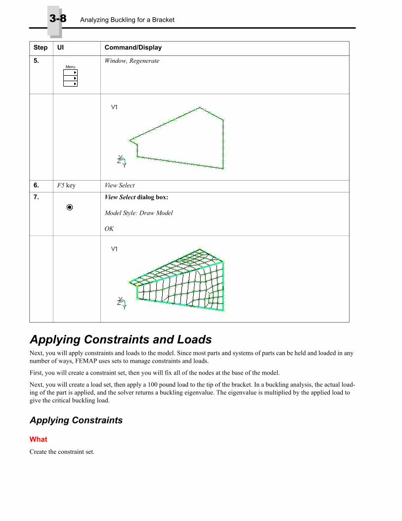
3-8 Analyzing Buckling for a Bracket
Applying Constraints and LoadsNext, you will apply constraints and loads to the model. Since most parts and systems of parts can be held and loaded in any number of ways, FEMAP uses sets to manage constraints and loads.
First, you will create a constraint set, then you will fix all of the nodes at the base of the model.
Next, you will create a load set, then apply a 100 pound load to the tip of the bracket. In a buckling analysis, the actual load-ing of the part is applied, and the solver returns a buckling eigenvalue. The eigenvalue is multiplied by the applied load to give the critical buckling load.
Applying Constraints
What
Create the constraint set.
5. Window, Regenerate
6. F5 key View Select
7. View Select dialog box:
Model Style: Draw Model
OK
Step UI Command/Display
Menu

Applying Constraints 3-9
How
WhatCreate the constraints to fix the nodes at the base of the model.
How
Step UI Command/Display
1. Model, Constraint, Create/Manage Set
2. Constraint Set Manager dialog box:
Click New Constraint Set, then...
3. New Constraint Set dialog box:
Title: (enter a title)
4. Click OK, then...
Constraint Set Manager dialog box:
Click Done
Step UI Command/Display
1. Model, Constraint, Nodal
2. Entity Selection dialog box:
Pick the nodes at the edge of the model.
OK
3. Create Nodal Constraints/DOF dialog box:
Fixed
OK
Cancel
Menu
Menu

3-10 Analyzing Buckling for a Bracket
4. Click View Visibility icon (on View Toolbar)
OR
Press Crtl+Q
5. Choose Labels radio button
6. Click All Off button, then...
Click Done
Notice: You can use the Entity Display Toolbar to quickly toggle Labels on and off. If the Entity Display Toolbar is not visible, you can turn it on using the Tools, Toolbars, Entity Dis-play command to make visible (shown “undocked”).
The third icon allows you to toggle Labels on and off.
Step UI Command/Display

Applying Loads 3-11
Applying LoadsApply the 100-pound load to the model.
What
Create the load set.
How
What
Create the load in the negative Y direction.
How
Step UI Command/Display
1. Model, Load, Create/Manage Set
2. Load Set Manager dialog box:
Click New Load Set, then...
3. New Load Set dialog box:
Title: (enter a title)
4. Click OK, then...
Load Set Manager dialog box:
Click Done
Step UI Command/Display
1. Model, Load, Nodal
2. Entity Selection dialog box:
Pick node at the tip of arrow (see following figure).
OK
Menu
Menu

3-12 Analyzing Buckling for a Bracket
Analyzing the ModelThe FEMAP analysis manager stores the options for creating an input file for a solver (an analysis set). It can launch the NX NASTRAN solver or another solver that has been set up to run on the same computer. The analysis manager, together with VisQ, can also set up and run analyses with solvers on other computers.
The analysis sets are stored with the FEMAP model file, and can also be stored in a FEMAP library that can be accessed from different model files.
What
Create the analysis set and solve the model.
3. Create Loads on Nodes dialog box:
FY: Value: 100
4. Click OK, then...
Click Cancel
Tip: Sometimes, it may be difficult to see a displayed load. If so, Force and Moment loads may be “reversed” to be have the “head” of the arrow on the selected node, point, or curve instead of the “tail”. To do this, press the F6 key to open the View Options dialog box, set Category to Labels, Entities and Color, then select Load Vectors from the list of Options. Finally, check “Reverse” and click OK.
Step UI Command/Display
A
XY
Z
V1C1
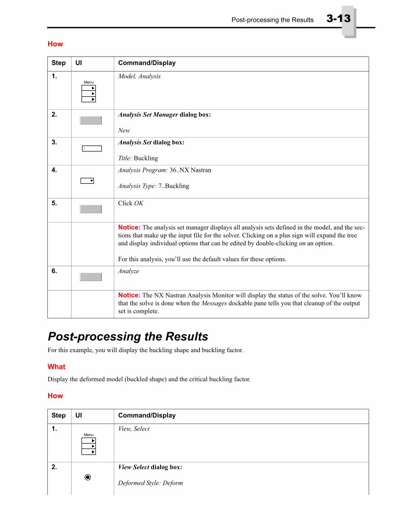
Post-processing the Results 3-13
How
Post-processing the ResultsFor this example, you will display the buckling shape and buckling factor.
What
Display the deformed model (buckled shape) and the critical buckling factor.
How
Step UI Command/Display
1. Model, Analysis
2. Analysis Set Manager dialog box:
New
3. Analysis Set dialog box:
Title: Buckling
4. Analysis Program: 36..NX Nastran
Analysis Type: 7..Buckling
5. Click OK
Notice: The analysis set manager displays all analysis sets defined in the model, and the sec-tions that make up the input file for the solver. Clicking on a plus sign will expand the tree and display individual options that can be edited by double-clicking on an option.
For this analysis, you’ll use the default values for these options.
6. Analyze
Notice: The NX Nastran Analysis Monitor will display the status of the solve. You’ll know that the solve is done when the Messages dockable pane tells you that cleanup of the output set is complete.
Step UI Command/Display
1. View, Select
2. View Select dialog box:
Deformed Style: Deform
Menu
Menu
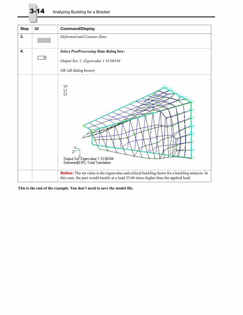
3-14 Analyzing Buckling for a Bracket
This is the end of the example. You don’t need to save the model file.
3. Deformed and Contour Data
4. Select PostProcessing Data dialog box:
Output Set: 2..Eigenvalue 1 33.06344
OK (all dialog boxes)
Notice: The set value is the eigenvalue and critical buckling factor for a buckling analysis. In this case, the part would buckle at a load 33.06 times higher than the applied load.
Step UI Command/Display

4. Analyzing a Beam Model
In this example, you’ll use rod and L beam elements to represent a truss structure.
You will work through the entire FEMAP analysis process, which includes:
• importing the geometry of the truss
• defining the material and property
• meshing the model using beams and rods
• applying constraints and loads
• analyzing the model using NX Nastran
• post-processing the results
Importing the Geometry
What
Open a new model file and import the geometry of the truss. These curves will be meshed with rod and beam elements.
How
Step UI Command/Display
1. File, Import, FEMAP Neutral
2. Read Model from FEMAP Neutral dialog box:
Go to the Examples directory in your FEMAP installation.
Truss.NEU
Open
OK
Menu

4-2 Analyzing a Beam Model
Defining the Material and PropertyThe first step for the meshing process will be to define the material and property for the beam and rod elements.
Defining the Material
What
Define the material by selecting a standard material from the FEMAP material library.
How
Defining the Beam PropertyFEMAP has a library of general cross sections for you to choose from, but you may not always want to use them. You can define an arbitrary cross section by creating a surface in FEMAP, or by importing external geometry. FEMAP will then cal-culate the section properties from that surface.
Step UI Command/Display
1. Model, Material
Tip: You can also create a new Material using the New command on the “context sensitive menu” located on the Materials branch in the Model Info tree (simply click to highlight the top level of the Materials branch or any existing Material, then right mouse click to see the context sensitive menu).
2. Define Material - ISOTROPIC dialog box:
Load
3. Select from Library dialog box:
AISI 4340 Steel
OK
OK, then...
Cancel
Step UI Command/Display
Menu

Defining the Beam Property 4-3
The neutral file that you imported has a boundary surface on a different layer that is not currently shown. You will now dis-play it.
What
First, hide the default layer. Next, display the boundary surface on a hidden layer.
How
What
Define a property for the beam elements. You’ll first create a general beam cross section, then define a vector to define the section’s Y axis. Next, you’ll define the beam property with the cross section and the AISI 4340 material that you’ve cre-ated.
How
Step UI Command/Display
1. Click View Visibility icon (on View Toolbar)
OR
Press Crtl+Q.
Visibility dialog box:
Choose the Layer tab.
2. CHECK “2..Beam Section”
UNCHECK “1..Default Layer”
3. Click Done
4. Ctrl - A Autoscale
Notice: The boundary section and curves are displayed.
Step UI Command/Display
1. Model, Property
XY
Z
Menu

4-4 Analyzing a Beam Model
Tip: You can also create a new Property using the New command on the “context sensitive menu” located on the Properties branch in the Model Info tree (simply click to highlight the top level of the Properties branch or any existing Property, then right mouse click to see the context sensitive menu).
2. Define Property dialog box:
Elem/Property Type
3. Element Property Type dialog box:
Line Elements: Beam
OK
4. Define Property - BEAM Element Type dialog box:
Shape
5. Cross Section Definition dialog box:
Shape: General Section
6. Surface
7. Select Surface to Check dialog box:
Click on the surface.
OK
8. Vector Locate - Define Section Y Axis dialog box:
Base: 0, 0, 0 (make sure these are the X,Y,Z values for the base)
Tip: 0, 1, 0 (enter these X,Y,Z values for the tip)
OK
Notice: This vector defines the Y axis for the section.
9. Cross Section Definition dialog box:
OK
10. Define Property dialog box:
Title: General Beam Section
Notice: The calculated section properties are now displayed in this dialog box.
11. Material: AISI 4340 Steel
OK, then...
Cancel
Step UI Command/Display

Meshing the Model 4-5
Meshing the ModelThis model will be meshed with two types of elements: beam elements on the longitudinal curves, and rod elements on the curves that connect the beams. Once you’ve created the elements, you’ll merge the coincident nodes.
Creating the Beam MeshFirst, mesh the longitudinal curves with beams whose properties were defined in the previous section.
What
Hide the beam section and show the default layer.
How
Step UI Command/Display
1. Click View Visibility icon (on View Toolbar)
OR
Press Crtl+Q.
2. CHECK “1..Default Layer”
UNCHECK “2..Beam Section”
3. Click Done
Tip: You can “hide and show” layers very easily using the Model Info tree. You can simply check or uncheck layers one at a time.
You can also select any number of layers using the Ctrl or Shift keys and the mouse. Once the layers are selected, right mouse on the “visibility check boxes” and choose the Show Selected, Show Selected Only, or the Hide Selected command.
You can also choose to View All Layers or View Visible Layers Only by selecting those com-mands from the “context sensitive menu” for Layers
4. Ctrl - A Autoscale
Step UI Command/Display

4-6 Analyzing a Beam Model
What
Rotate the model to get a trimetric view for meshing.
How
What
Mesh the longitudinal curves with beams. You’ll use the general beam cross section to define the beam. After you select the cross section, you’ll enter a vector to define the beam element orientation. It’s important that this vector be identical to the one used to define the cross section properties; otherwise, your analysis results may be incorrect.
How
Step UI Command/Display
1. View, Rotate, Model
Tip: You can press the F8 key instead of using the command above.
2. View Rotate dialog box:
Trimetric
OK
Step UI Command/Display
1. Mesh, Geometry, Curve
2. Entity Selection dialog box:
Pick the curves highlighted in the following figure (Curve IDs 7, 8, 9, 11, 12, 13, 14, 15, 24, 25, 26, 28, 29, 30, 31, and 32).
OK
Step UI Command/Display
Menu
Menu

Creating the Beam Mesh 4-7
What
Display the beam elements with their cross sections visible.
How
3. Geometry Mesh Options dialog box:
Property: General Beam Section OK
4. Vector Locate dialog box:
Base: 0, 0, 0 (make sure these are the X, Y, Z values for the base)
Tip: 0, 1, 0 (enter these X, Y, Z values for the tip)
OK
Step UI Command/Display
1. F6 key View Options
2. View Options dialog box:
Category: Labels, Entities, and Color
Option: Element Orientation/Shape (select)
Element Shape: Show Cross Section (select)
OK
Step UI Command/Display
XYZ
V1

4-8 Analyzing a Beam Model
What
Rotate and zoom the model to get a better look at the cross section. Your cross section may have an incorrect orientation that you need to modify.
How
Tip: You can also “toggle” the cross-sections of line elements on/off using the “Thickness/Cross Section” command from the View Style menu located on the View Toolbar.
Step UI Command/Display
1. Rotate the model slightly to the see the cross sections better.
2. Zoom (on View Toolbar)
Notice: Compare your beams with the following diagram. If some of your beams are ori-ented differently, you will need to modify them. The following steps show you how to reverse the normals when they are facing in the wrong direction.
It is normal for you to need to modify the normal direction of some of your beams to make it look like the figure below.
Step UI Command/Display

Creating the Rod Mesh 4-9
Creating the Rod MeshYou will now mesh the remaining curves with rod elements to connect the beams.
What
Mesh the curves. You’ll also need to create a new property to define the rods.
How
3. Modify, Update Elements, Line Element Reverse Direction
4. Entity Selection dialog box:
Pick the elements to modify. (Pick only the elements with cross sections facing in the wrong direction.)
OK
5. In Update Element Direction dialog box:
Reverse Direction
OK
6. Ctrl - A Autoscale
Step UI Command/Display
1. Mesh, Geometry, Curve
Step UI Command/Display
Menu
Menu

4-10 Analyzing a Beam Model
What
Reduce the amount of information displayed by turning off the display of geometry and labels.
2. Entity Selection dialog box:
Pick all of the unmeshed curves: the cross braces and the connection between the two rows of beams.
OK
3. Geometry Mesh Options dialog box:
Property “icon button”
Notice: You only have the General Beam Section property in your model. You’ll need to create a rod property.
4. Define Property dialog box:
Elem/Property Type
5. Line Elements: Rod
OK
6. Define Property - ROD Element Type dialog box:
Title: 2 inch Diameter Rod
Area: 3.14
7. Material: AISI 4340 Steel
OK
8. Geometry Mesh Options dialog box:
OK
Notice: The property you created is selected for the element’s property.
Notice: The curves are meshed with rod elements.
Step UI Command/Display
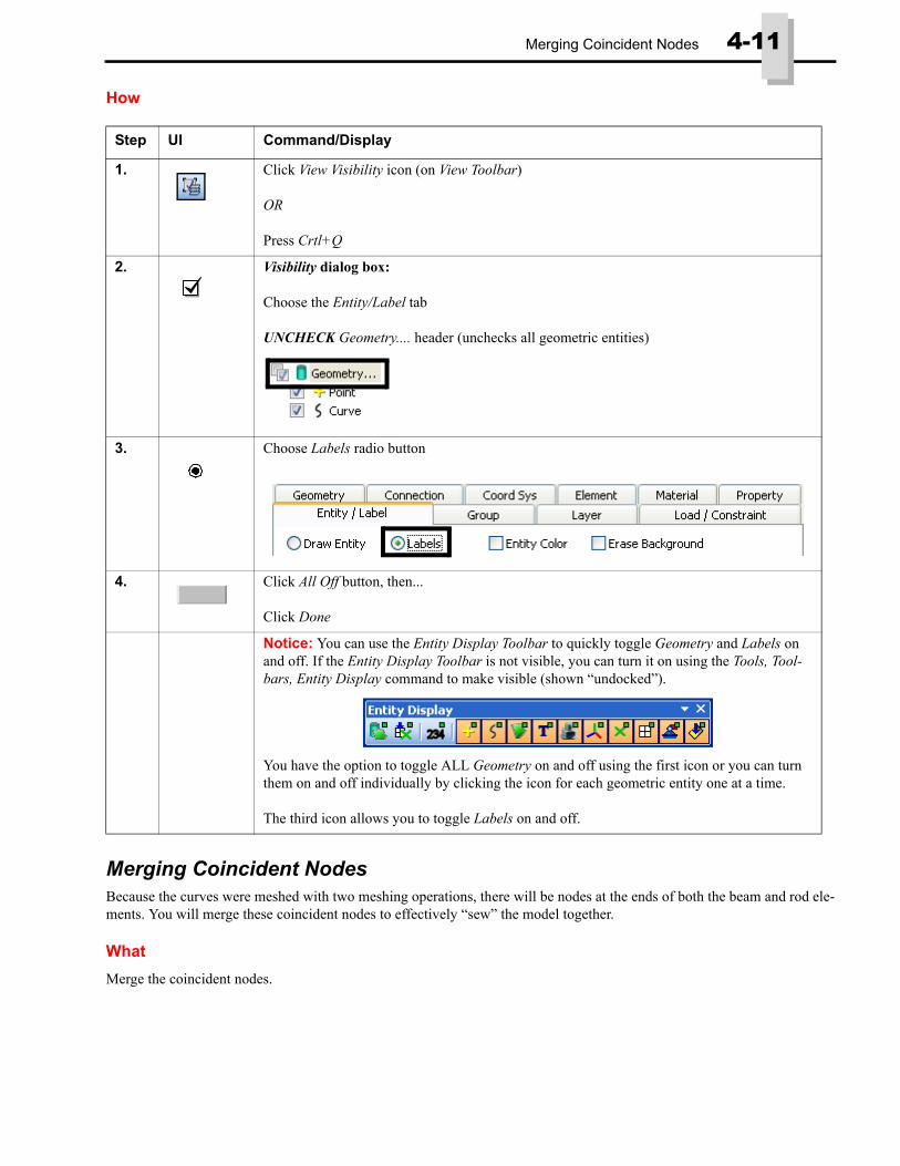
Merging Coincident Nodes 4-11
How
Merging Coincident NodesBecause the curves were meshed with two meshing operations, there will be nodes at the ends of both the beam and rod ele-ments. You will merge these coincident nodes to effectively “sew” the model together.
What
Merge the coincident nodes.
Step UI Command/Display
1. Click View Visibility icon (on View Toolbar)
OR
Press Crtl+Q
2. Visibility dialog box:
Choose the Entity/Label tab
UNCHECK Geometry.... header (unchecks all geometric entities)
3. Choose Labels radio button
4. Click All Off button, then...
Click Done
Notice: You can use the Entity Display Toolbar to quickly toggle Geometry and Labels on and off. If the Entity Display Toolbar is not visible, you can turn it on using the Tools, Tool-bars, Entity Display command to make visible (shown “undocked”).
You have the option to toggle ALL Geometry on and off using the first icon or you can turn them on and off individually by clicking the icon for each geometric entity one at a time.
The third icon allows you to toggle Labels on and off.

4-12 Analyzing a Beam Model
How
Applying Constraints and LoadsYou will create a constraint set to model symmetry and fix the end. The symmetry of the truss will be used to reduce the model to half the size.
You will also apply a load to this model to simulate something hanging from the truss.
Modeling Symmetry and a Fixed EndTo simulate the symmetry of this part, you will constrain the four nodes that are at the halfway point of the structure. You are defining symmetry across the X-plane through these four points. By imposing this type of constraint condition, you are actually introducing a stiffness exactly equal to the structure modeled, just mirrored above the X-plane.
What
Create the constraints to model symmetry and fix the end. You’ll also constrain the rest of the model in all DOF except the X and Y translations.
How
Step UI Command/Display
1. Tools, Check, Coincident Nodes
2. Entity Selection dialog box:
Select All
OK
3. Check/Merge Coincident dialog box:
Action: Merge
Keep ID: Automatic
Move To: Current Location
4. OK
Notice: Look in the Messages dockable pane to see how many coincident nodes have been merged. All rod and beam elements are now connected together.
Step UI Command/Display
1. View, Rotate, Model
Tip: You can press the F8 key instead of using the command above.
Menu
Menu

Modeling Symmetry and a Fixed End 4-13
2. View Rotate dialog box:
Isometric
OK
3. Model, Constraint, Nodal
Notice: First, you’ll apply constraints at these nodes to model symmetry.
4. New Constraint Set dialog box:
Title: (enter a title)
OK
5. Entity Selection dialog box:
Pick nodes A, B, C, and D (see the following figure).
OK
6. Create Nodal Constraints/DOF dialog box:
X Symmetry
7. Title: X Symmetry
8. OK
Notice: The TX, RY, and RZ DOF are selected.
Because you are applying nodal constraints, you could control the constraint of each degree of freedom individually in the dialog box, or you can use the quick keys to apply common constraint conditions.
Step UI Command/Display
Menu
A
B
D
C

4-14 Analyzing a Beam Model
9. Entity Selection dialog box:
Pick nodes E and F (see the following figure).
OK
Notice: You are now fixing the nodes on the opposite end.
10. Create Nodal Constraints/DOF dialog box:
Fixed
11. Title: Fixed
12. OK
Notice: All DOF are selected.
13. Entity Selection dialog box:
Select All
OK
Notice: Finally, you’ll restrain the DOF for all nodes in the Z translation and all rotations.
14. Create Nodal Constraints dialog box:
DOF: TZ, RX, RY, RZ (check)
OK
15. Title: Singularity Constraints
16. OK
No (to combine the constraints)
Entity Selection dialog box:
Cancel
Step UI Command/Display
F
E

Applying a Load to the Model 4-15
What
Turn off element cross sections to better see the constraints.
How
Applying a Load to the ModelYou will now apply a load in the negative Y direction to simulate something hanging from this truss. Like constraints, loads are grouped in sets. Before creating any loads, you must create a set to hold them.
What
Create the load in the negative Y direction.
How
Step UI Command/Display
1. F6 key View Options
2. View Options dialog box:
Category: Labels, Entities and Color
3. View Options dialog box:
Options: Element Orientation/Shape (select)
Element Shape: Line/Plane Only (select)
OK
Tip: If you turn the constraint labels back on, you’ll see the degree of freedom numbers dis-played for each constraint. (To do this, pick F6. Pick Options, Constraint. Under Label Mode, pick Degree of Freedom.)
Step UI Command/Display
1. Model, Load, Nodal
Menu
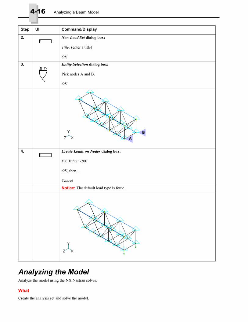
4-16 Analyzing a Beam Model
Analyzing the ModelAnalyze the model using the NX Nastran solver.
What
Create the analysis set and solve the model.
2. New Load Set dialog box:
Title: (enter a title)
OK
3. Entity Selection dialog box:
Pick nodes A and B.
OK
4. Create Loads on Nodes dialog box:
FY: Value: -200
OK, then...
Cancel
Notice: The default load type is force.
Step UI Command/Display
B
A

Post-Processing the Results 4-17
How
Post-Processing the ResultsFor this example, you will display three types of results: criteria plots, beam diagrams, and stresses on beam cross sections.
Displaying Criteria DiagramsAs an alternative to contours, you can use a basic criteria display that shows the output value of each element. The primary purpose of a criteria display, however, is to limit the display based on a selected criteria.
What
Display a basic criteria view of the results.
How
Step UI Command/Display
1. Model, Analysis
2. Analysis Set Manager dialog box:
New
3. Analysis Set dialog box:
Title: (enter a title for the solve)
4. Analysis Program: 36..NX Nastran
Analysis Type: 1..Static
OK
5. Analyze
Step UI Command/Display
1. F5 key View Select
2. View Select dialog box:
Deformed Style: Deform
Contour Style: Criteria
3. Deformed and Contour Data
Menu

4-18 Analyzing a Beam Model
What
To reduce clutter, turn off display of undeformed elements.
How
4. Select PostProcessing Data dialog box:
Output Vectors: Deform: 1..Total Translation
Contour: 3022..Beam EndA Axial Force
OK (all dialog boxes)
5. View, Rotate, Model
Tip: You can press the F8 key instead of using the command above.
6. View Rotate dialog box:
Trimetric
OK
Step UI Command/Display
1. F6 key View Options
Step UI Command/Display
Menu

Displaying Criteria Diagrams 4-19
What
Modify the criteria for the elements to be displayed. Display the elements above the maximum limit of 350.
How
2. View Options dialog box:
Category: PostProcessing
3. Options: Undeformed Model
4. UNCHECK Draw Entity
OK
Step UI Command/Display
1. F6 key View Options
2. View Options dialog box:
Notice: The PostProcessing category is already selected.
3. Options: Criteria Limits
Step UI Command/Display
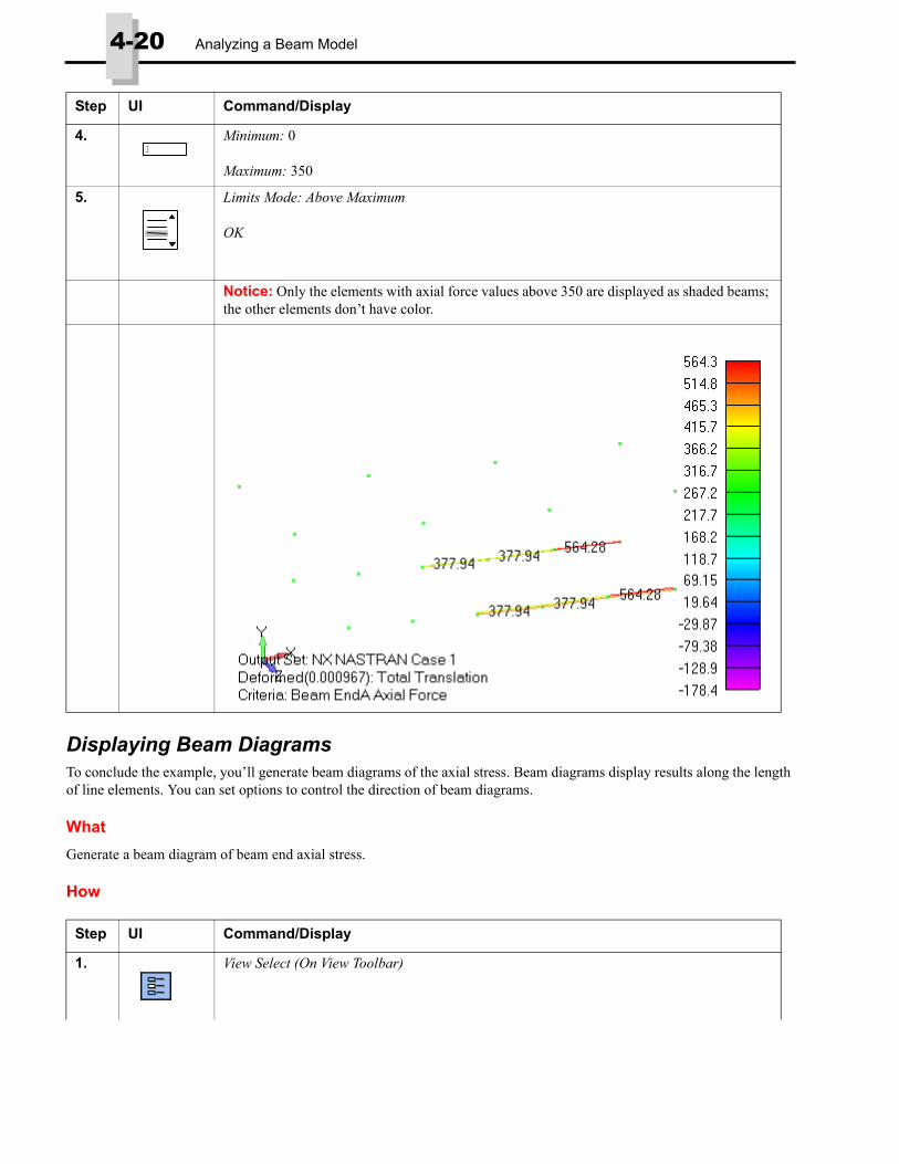
4-20 Analyzing a Beam Model
Displaying Beam DiagramsTo conclude the example, you’ll generate beam diagrams of the axial stress. Beam diagrams display results along the length of line elements. You can set options to control the direction of beam diagrams.
What
Generate a beam diagram of beam end axial stress.
How
4. Minimum: 0
Maximum: 350
5. Limits Mode: Above Maximum
OK
Notice: Only the elements with axial force values above 350 are displayed as shaded beams; the other elements don’t have color.
Step UI Command/Display
1. View Select (On View Toolbar)
Step UI Command/Display

Displaying Beam Diagrams 4-21
What
You can change the plane where the beam diagram will be drawn. FEMAP always draws the diagram in the plane that you choose, even if the output is actually based on forces/stresses in a different plane.
How
2. View Select dialog box:
Deformed Style: None - Model Only
Contour Style: Beam Diagram
3. Deformed and Contour Data
4. Select PostProcessing Data dialog box:
Contour: 3139..Beam EndA Pt1 Comb Stress
OK (all dialog boxes)
Step UI Command/Display
1. F6 key View Options
2. View Options dialog box:
Options: Beam Diagram
Default Direction: Element Z
OK
Step UI Command/Display

4-22 Analyzing a Beam Model
What
Interactively view calculated stresses on the cross-section of beam elements.
How
Notice: The beam diagrams are now drawn on the element Z plane.
Step UI Command/Display
1. View Select (On View Toolbar)
2. View Select dialog box:
Contour Style: None - Model Only
3. OK
4. View, Advanced Post, Beam Cross Section
5. In Beam Cross Section Stress Control dialog box:
Select Single in Elements section
Step UI Command/Display
Menu

Displaying Beam Diagrams 4-23
6. Click in text field next to Single, then...
Pick Element 2 (Top row, towards back of model, middle element).
7. In Location section:
Position: 85
8. Select Screen Space radio button
A plot of the Axial Stress on the cross section of the beam should now appear while the dialog box is still displayed.
9. In Location section:
Select Model Space radio button
Step UI Command/Display

4-24 Analyzing a Beam Model
Shown zoomed in for clarity
10. In Location section:
Move the slider bar between End A and End B.
This will dynamically change the results for a single element when set to Screen Space or Model Space.
11. Position: 50
12. Select Screen Space radio button
13. In Show Stress section:
Select Combined Shear from drop-down
14. CHECK Vector Plot option
15. Click Advanced button
16. In Advanced Options dialog box:
In Vector Plot Options section:
UNCHECK Solid Vector option
CHECK Section Outline
Step UI Command/Display

Displaying Beam Diagrams 4-25
This is the end of this example. You don’t need to save the model file.
17. Vector Length: 80
18. OK (All dialog boxes)
Notice: Once the view is Redrawn or Regenerated, the graphics window will revert back to showing the model with no Beam Cross Section stresses displayed. To display the stresses again using the same options, simply choose the View, Advanced Post, Beam Cross Section command again.
Step UI Command/Display

4-26 Analyzing a Beam Model

5. Analyzing a Midsurface Model of an Electrical Box
In this example, you will learn to work with FEMAP’s semi-automatic midsurface extraction capabilities to build an ideal-ized model of an electrical box.
To work through this example, you must have a licensed copy of NX Nastran for FEMAP. You will not be able to complete this example with the 300-node demo version.
The example includes the following steps:
• importing the geometry using the STEP interface
• creating the midsurface model
• meshing the model
• applying loads and constraints
• analyzing the model using NX Nastran
• post-processing the results
Importing the GeometryTo begin the example, you will import the geometry.
What
Start FEMAP and open a new model file. Import the STEP file.
How
Step UI Command/Display
1. File, Import, Geometry
Go to the Examples directory in your FEMAP installation.
Import the mp.STP file.
Menu

5-2 Analyzing a Midsurface Model of an Electrical Box
Creating the Midsurface ModelCreate the midsurface model, then delete the original solid. Once the midsurface has been generated, you will need to so some additional cleanup work on the geometry before you can mesh it.
Creating the Midsurface
What
Use the automatic midsurfacing capability to create a midsurface model.
How
2. STEP Read Options dialog box:
OK
3. View, Rotate, Model
Tip: You can press the F8 key instead of using the command above.
4. View Rotate dialog box:
Dimetric
OK
5. View Style Menu (on View Toolbar)
Choose Wireframe
Step UI Command/Display
1. Zoom and rotate the part to get a better view of the points we will be picking to designate the “Target Distance” for midsurfacing.
Step UI Command/Display
Menu

Creating the Midsurface 5-3
2. Geometry, Midsurface, Automatic
3. Entity Selection dialog box:
Select All
OK
4.
OR Ctrl-D
In the Mid-Surface Tolerance dialog box:
Click the Measure Distance icon button or press Ctrl-D on the keyboard. Doing either will open FEMAP’s distance measuring tool.
Notice: The Measure Distance icon button or Ctrl-D command lets you determine distance for the target thickness.
The software uses this value to determine which surfaces to place a midsurface between. The target thickness should be slightly larger than the largest distance between the planes on the solids that you want midsurfaced. If the target thickness is too low, the midsurfaces will not be created. If the target thickness is too high, some midsurfaces will be created between the wrong surfaces.
5. Locate dialog box:
Methods
6. On Point
7. On Point dialog box:
Pick point A (see following figure).
OK
Step UI Command/Display
Menu

5-4 Analyzing a Midsurface Model of an Electrical Box
8. Pick point B.
OK
9. Midsurface Tolerance dialog box:
CHECK pre-v11.1 Midsurface Method box located in the Midsurface Options section
Notice: The pre-V11.1 Midsurface Method is used in this example because it presents the additional tools available for modifying midsurfaces should the Geometry, Midsurface, Automatic command not create a full satisfactory midsurface representation. For instance, the desired surfaces may not be created or some surfaces may need to be manually altered. Please try the example again without turning on the pre-V11.1 Midsurface Method option to see what the enhanced face pairing algorithm does using this geometry.
10. OK (accept the value calculated by the Measure Distance command)
Notice: The target thickness value should be approximately 4.93.
Step UI Command/Display
XYZ
V1
AB
XYZ
V1

Deleting the Solid 5-5
Deleting the SolidWhat
Delete the original solid.
How
Cleaning Up the GeometryTo create a more accurate midsurface model, you must trim each rib, then delete the top portion.
Step UI Command/Display
1. Delete, Geometry, Solid
2. Entity Selection dialog box:
ID: 1
OK
OK
3. View Style Menu (on View Toolbar)
Choose Solid
Menu
Back
Front

5-6 Analyzing a Midsurface Model of an Electrical Box
What
Trim the surface of each rib.
How
Step UI Command/Display
1. Geometry, Midsurface, Trim with Curve
2. Select Surface/Solid to Trim dialog box:
Pick one of the eight ribs.
OK
3. Entity Selection dialog box:
Pick the curve on the lower portion (see C above).
OK
Notice: The curve now cuts through the surface.
Menu
C

Cleaning Up the Geometry 5-7
What
Delete the top portion of each rib.
How
4. Repeat the process to trim the other seven ribs.
Tip: You can rotate the model by holding down the middle mouse button and moving the mouse.
Step UI Command/Display
1. Delete, Geometry, Surface
2. Entity Selection dialog box:
Pick the new surfaces that have been created on the top of each rib (see D in the following figure).
OK
OK
Notice: The top of each rib has been deleted.
Step UI Command/Display
Menu
D

5-8 Analyzing a Midsurface Model of an Electrical Box
What
.Intersect the new ribs with the walls of the electric box.
How
Meshing the ModelThe first step in meshing the model is to assign mesh attributes for the different surfaces. If the correct attributes are not assigned, the results won’t be correct.
Next, set the size for the mesh. Finally, mesh the midsurface.
Assigning Mesh Attributes
What
Assign the mesh attributes to the surfaces.
How
Step UI Command/Display
1. Geometry, Midsurface, Intersect
2. Entity Selection dialog box:
Select All
OK
Step UI Command/Display
1. Geometry, Midsurface, Assign Mesh Attributes
2. Entity Selection dialog box:
Select All
OK
3. Define Material - ISOTROPIC dialog box:
Load
4. In Select from Library dialog box:
AISI 4340 Steel
OK
Menu
Menu

Meshing the Model 5-9
Meshing the Model
What
Set the mesh size to the default value, then mesh the model.
How
5. “OK to Consolidate Properties by Thickness?” question box:
No
Notice: Each surface now has a Plate property and a material assigned to it. Clicking Yes would have minimized the number of new properties created based on similar thickness.
Tip: If midsurfaces are created manually using commands such as Geometry, Surface, Off-set or Geometry, Surface, Extrude, the surfaces do not have mesh attributes. You must man-ually assign mesh attributes by creating or assigning existing properties using the correct thickness.
Step UI Command/Display
1. Mesh, Mesh Control, Size on Surface
2. Entity Selection dialog box:
Select All
OK, then...
Automatic Mesh Sizing dialog box:
OK, then...
Cancel
3. Mesh, Geometry, Surface
4. Entity Selection dialog box:
Select All
OK, then...
Automesh Surfaces dialog box:
OK
Step UI Command/Display
Menu
Menu

5-10 Analyzing a Midsurface Model of an Electrical Box
Applying Loads and ConstraintsTo load the model, you will apply a pressure to the surface at the back of the part. You will also constrain the holes at the base.
5. Click View Visibility icon (on View Toolbar)
OR
Press Crtl+Q
6. Visibility dialog box:
Choose the Entity/Label tab
Choose Draw Entity radio button
7. UNCHECK Node box located in the Mesh section,
UNCHECK the “top-level” box for Geometry
then...
8. Click Done
Step UI Command/Display

Applying Loads and Constraints 5-11
What
Create a load set, the apply a pressure to the back of the part.
How
Step UI Command/Display
1. Model, Load, On Surface
2. Because no load sets exist in the model, FEMAP will prompt you to create one
New Load Set dialog box:
Title: (enter a title)
3. Click OK
4. Entity Selection dialog box:
ID: The middle surface at the back of the part. It may have a different Surface ID (usually ID is 129)OK
5. Click OK
6. Create Loads on Surfaces dialog box:
Pressure
7. Pressure: Value: -1
OK, then...
Cancel
Menu

5-12 Analyzing a Midsurface Model of an Electrical Box
What
Constrain the holes at the bottom of the part.
How
Analyzing the ModelSolve the model using the NX Nastran solver.
Step UI Command/Display
1. Model, Constraint, On Curve
2. Because no constraint sets exist in the model, FEMAP will prompt you to create one
New Constraint Set dialog box:
Title: (enter a title)
3. Click OK
4. Entity Selection dialog box:
Pick the eight curves around the holes at the base.
OK
Tip: You may want to rotate the model and zoom in on the corners of the model to make selection of these curves easier. While in a command you can use the middle mouse button to rotate the model as well as the Zoom and Previous Zoom icons on the View Toolbar.
5. Create Constraints on Geometry dialog box:
Pinned - No Translation
OK, then...
Cancel
Tip: To see the nodes and elements on which the loads and constraints are applied, use the Model, Load, Expand and Model, Constraint, Expand commands.
Menu
XYZ
TTT
T
V1L1C1

Post-processing the Results 5-13
What
Create the analysis set and solve the model.
How
Post-processing the ResultsFor this analysis, you will display deformation and stress contours.
What
Display and deformed/contour plot of translation and stress.
How
Step UI Command/Display
1. Model, Analysis
3. New
2 Analysis Program: 36..NX Nastran
Analysis Type: 1..Static
OK
3. Analyze
Step UI Command/Display
1. F5 key View Select
2. View Select dialog box:
Deformed Style: Deform
Contour Style: Contour
3. Deformed and Contour Data
4. Select PostProcessing Data dialog box:
Output Vectors: Deform: 1..Total Translation
Output Vectors: Contour: 7026..Plate Top MajorPrn Stress
OK (all dialog boxes)
Menu

5-14 Analyzing a Midsurface Model of an Electrical Box
5. Rotate the model so that you can see the back.
Notice: You can see the plate top stress contour on both faces of the plate elements.
Step UI Command/Display

Post-processing the Results 5-15
What
Change the contour options to display double-sided planar contours.
If you select a standard top or bottom plate vector for contouring, as you did above, FEMAP can automatically contour both top and bottom stresses on the same plot.
How
Step UI Command/Display
1. F5 key View Select
2. View Select dialog box:
Deformed and Contour Data
3. Select PostProcessing Data dialog box:
Output Vectors: Double-Sided Planar Contours
Notice: Because the default for contours in FEMAP is to “Match Output” (i.e., show nodal results as nodal contours and elemental results as elemental contours), the following com-mands are not really required to get the desired plot. They are simply shown as a reference should you want to use a specific Contour Type (Nodal, Elemental, or Match Output), change the method of Data Conversion (Average, Maximum, or Minimum), or toggle Use Corner Data on/off.
4. Contour Options
5. Select Contour Options dialog box:
Contour Type: Elemental
6. Data Conversion: Average
7. Data Selection: CHECK Use Corner Data
8. OK (All dialog boxes)
Notice: The display has changed. The contour now shows plate top major principle stress on the top face of the plate elements and plate bottom major principle stress on the bottom face of the plate elements.

5-16 Analyzing a Midsurface Model of an Electrical Box
What
To more easily see double-sided results, change the view to show the element thicknesses.
9. Rotate the model to look at the back.
Notice: The contour on the back of the part shows plate top major stress.
Step UI Command/Display

Post-processing the Results 5-17
How
This is the end of the example. You don’t need to save your model file.
Step UI Command/Display
1. F6 key View Options
2. View Options dialog box:
Category: Labels, Entities and Color
3. Options: Element - Orientation/Shape, then...
Element Shape: 1..Show Fiber Thickness
4. Category: Tools and View Style
5. Options: Filled Edges
6. UNCHECK Draw Entity
OK
Tip: You can also toggle the “Filled Edges” and the “Thickness/Cross Section” on and off very easily using the View Style menu located on the View Toolbar. Simply select Filled Edges or Thickness/Cross Section from the View Style menu to turn them off, then select the command again to turn them back on at any time.
.Notice: The contour on the back of the part shows plate top major stress

5-18 Analyzing a Midsurface Model of an Electrical Box

6. Analysis of a Simple Assembly
In this example, you will create a model of a simple assembly using contact conditions automatically generated by FEMAP, then solve the model two times using NX Nastran, once using “Glued Contact” and once using “Linear Contact”.
Also, this example makes extensive use of the Model Info tree and Select Toolbar.
You will work through the entire FEMAP analysis process, which includes:
• importing the geometry of the assembly
• creating connections between different parts of the assembly
• meshing the model
• applying loads and constraints
• analyzing the model using the NX Nastran solver (Static Analysis using Glued and Linear Contact)
• post-processing the results
Importing the Geometry
What
Import a FEMAP geometry file containing the geometry of the assembly.
How
Step UI Command/Display
1. File, Import, Geometry
Go to the Examples directory in your FEMAP installation.
Import the Assembly.x_t file.
Menu

6-2 Analysis of a Simple Assembly
Creating ConnectionsYou will be creating connections between the different parts of the assembly. In this example, the connections will be con-tact conditions which NX Nastran will use during the solving process to have the parts interact with one another.
In general, there are three separate entities needed to create a connection in FEMAP:
Connection Property - A specific property used to set-up contact conditions for a specific solver or analysis type. We will be using the “NX Linear” tab and the Defaults button for this example.
Connection Regions - Regions designated in the model which can be placed into contact with any number of other regions. Regions can be created using different types of entities such as surfaces, elements, and properties. In this example, you will create contact between the different solid parts using the surfaces of those solids.
Connectors - Connectors create “contact pairs” between Connection Regions (using a Master/Slave relationship) and the contact between those regions is governed by the values set in the specified Connection Property for each Connector.
Each of these entities can be created individually using the Connect menu, but FEMAP offers a few methods for creating them in a more streamlined manner. One method is to use the Connect, Surfaces command which simply allows you to choose a surface (or set of surfaces) to “connect” to another surface (or set of surfaces). The surfaces in each set will be used to create the Connection Regions, a Connection Property can be chosen (or created from inside this command), and then a single Connector will be created between the selected surfaces.
2. Solid Model Read Options dialog box:
OK
3. View, Rotate, Model
Tip: You can press the F8 key instead of using the command above.
4. View Rotate dialog box:
Click Trimetric, then...
Click OK
Step UI Command/Display
Menu

Automatic Connection Creation 6-3
In this example, we will be using the Connect, Automatic command. This creates connections automatically based on the proximity of geometric entities selected in your model using a number of parameters. These parameters include specific val-ues for Tolerance (distance between bodies) and Angle Tolerance, as well as choice of a “Detection Strategy” (Minimal to Aggressive) and options for the way multiple Connection Regions will be combined on the same solid.
Automatic Connection Creation
What
Create connections automatically between the parts of the assembly.
How
Step UI Command/Display
1. Connect, Automatic...
2. Entity Selection - Select Solid(s) to Detect Connections dialog box:
Click Select All, then...
Click OK
Auto Detection Options for Connections dialog box: The following values should be selected:
If it does not, make sure all of the above options are chosen. Then...
3. Click OK
Entity Selection - Select Solid(s) to Detect Connections dialog box:
Click Cancel
Menu

6-4 Analysis of a Simple Assembly
You will notice the there are new Connection Regions which are visible where the parts come together.
You can take a closer look at each Connection Property, Connection Region, and Connector created using the Connections branch of the Model Info tree.
Examining Created ConnectionsUsing a few “context sensitive menu” commands from the Connections branch of the Model Info tree, you can graphically see the different Connection Regions and Connectors which were created by the Connect, Automatic command. If it is not open, you will need to have the Model Info tree open for this step.
What
Use the Model Info tree to examine the connections in the model.
Tip: Creating connections automatically can also be accomplished by using the “context sen-sitive menu” for the Geometry branch in the Model Info tree. Simply highlight the top-level Geometry branch in the tree (or individual solids), then click the right mouse button and choose Automatic Connection from the menu. This will bring up the Connect, Automatic command
Step UI Command/Display

Examining Created Connections 6-5
How
Step UI Command/Display
1. If the Model Info tree is NOT already open, you can bring it up using the Tools, Model Info command to make it visible.
Tip: If you are not familiar with the Model Info tree or the other “dockable panes” in FEMAP, you can find more information about them using the Help, Dockable Panes... menu.
The “dockable panes” contain a tremendous amount of features. It is highly recommended to review the documentation for these very helpful tools.
2. Model Info tree:Expand the Connections branch (click on the “+” sign to the right of the title) to see the differ-ent Connection entities
You will notice that Connection Properties, Connection Regions, and Connectors are all available in the Model Info tree.
3. Expand the Connectors branch to view the Connectors in the model
You will notice that two Connectors were created in the model by the automatic contact detection. They are listed in the following format:
#(number of Connector)..Region “#-#” (“Master/Target” Connection Region - “Slave/Source” Connection Region).
Highlight “1..Region 1-2” by clicking on it.
Menu

6-6 Analysis of a Simple Assembly
4 Click the right mouse button on the highlighted Connector. When the context sensitive menu appears, choose the Show Master (Target) command.
You will notice that the “Master/Target” Connection Region of Connector “1” has been highlighted in Yellow and the rest of the parts have been made transparent in the model. If your display does not look like the one below, please see the “notice” below this cell.
The model will remain in this display state until Windows, Regenerate (Ctrl+G) or Windows, Redraw (Ctrl+G) has been used or a command which includes a “Regenerate” or “Redraw” (such as an entity creation command) has been performed.
Notice: The Show Master (Target) and Show Slave (Source) commands follow the current settings in the Windows, Show Entities command. By default, nothing is set in FEMAP and you will get the figure above when using the Show Master (Target) and Show Slave (Source) commands.
If you have changed any of the settings in the Windows, Show Entities command itself or the Show When Selected commands in the Model Info tree or Data Table, then the Show Master (Target) and Show Slave (Source) commands will use those settings.
Step UI Command/Display

Examining Created Connections 6-7
5 Click the right mouse button on the highlighted Connector. When the context sensitive menu appears, choose the Show Slave (Source) command.
Tip: Although not needed for this model, in some cases you may want to “swap” the “Master/Target” and “Slave/Source” Connection Regions for an individual Connector. This can be accomplished by using the Reverse command in the Connectors context sensitive menu
Tip: It is also possible to “Enable” and “Disable” Connectors. This allows you to choose which Connectors will be exported for analysis. With this capability, you do not have to delete and recreate Connectors when determining which parts should come into contact in certain scenarios.
Step UI Command/Display

6-8 Analysis of a Simple Assembly
Applying Loads and Constraints For loads, create a load on front surface of the “Plunger”, normal to the surface. Next, create a “pinned” boundary condition using the surfaces of the rear holes of the “Baselink”.
What
Create a load set, then apply a force “normal” to the front surface of the “Plunger”.
How
Step UI Command/Display
1. Model, Load, Create/Manage Set
2. Load Set Manager dialog box:
Click New Load Set, then...
3. New Load Set dialog box:
Title: “Normal Force”
4. Click OK, then...
Load Set Manager dialog box:
Click Done
For the selection of the surface to load, use the Select Toolbar (Shown undocked)
If the Select Toolbar is not visible, you can make it visible using the Tools, Toolbars, Select command or by right-mouse clicking in any area where a toolbar can be “docked” and choos-ing Select from menu. For more information on where a toolbar can be “docked”, please use the Help, Toolbars, Using the Toolbars command to view the documentation.
All of the icons on the Select Toolbar are actually menus which allow you to modify the way the Select Toolbar will be used. For more information on the Select Toolbar, please view the documentation using the Help, Toolbars, Select command.
Menu

Applying Loads and Constraints 6-9
5. Using the Selector Entity menu on the Select Toolbar (first icon), select Surface. You will notice that the icon on the Select Toolbar has changed to the Select Surface icon.
This will make Surfaces “Active” in the Selector. Having an “Active” entity in the Selector allows you to choose Surfaces in the model before selecting any commands. In this case you will only be selecting one surface at a time, but there are options for selecting multiple sur-faces, then choosing commands. This also will give you access to the “context sensitive menu” for the “Active” Entity Type in the graphics window.
6. With Surface “Active” in the Select Toolbar:
Pick the front round surface of the “Plunger” (surface 36).
If you turn on the Entity Info dockable pane, you will be able to see which surfaces you are choosing as you pick them. Use the Tools, Entity Info command to open up this pane.
Note: The surface will NOT change color (This has been done for this example to show which surface to select), but the small “Selected Marker” (circle in above figure) will appear in FEMAP to let you know the surface has been selected.
7. Click the right mouse button on the highlighted Surface or anywhere in the graphics window. When the “context sensitive menu” appears, choose the Load command.
This will bring up the Create Loads on Surfaces dialog box.
Step UI Command/Display
Menu

6-10 Analysis of a Simple Assembly
Tip: When the Select Toolbar has an “Active” entity type, a right mouse click in the graphics window will always bring up the “context sensitive menu” for the “Active” Entity Type.
Because of this, you will not be able to use the “normal right-mouse menu” simply by click-ing the right-mouse button. Instead you have to hold down the Alt key, then click the right-mouse button to get to the Quick Access Menu (“normal right-mouse menu”). When there is no longer an “Active” Entity Type in the Select Toolbar, holding down Alt is not required.
Tip: You can also use icons from various toolbars to perform commands on the entities cur-rently in the Selector. In this case, you could have used the Create Load on Surface icon on the Loads Toolbar.
8. Create Loads on Surfaces dialog box:
Highlight Force from the selection list
9. In Direction section, select Normal to Surface
10. Enter “100” in Magnitude field of the Load section
11. Click OK
Step UI Command/Display
Create Load on Surface icon
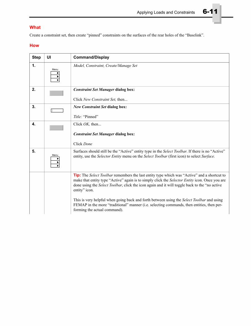
Applying Loads and Constraints 6-11
What
Create a constraint set, then create “pinned” constraints on the surfaces of the rear holes of the “Baselink”.
How
Step UI Command/Display
1. Model, Constraint, Create/Manage Set
2. Constraint Set Manager dialog box:
Click New Constraint Set, then...
3. New Constraint Set dialog box:
Title: “Pinned”
4. Click OK, then...
Constraint Set Manager dialog box:
Click Done
5. Surfaces should still be the “Active” entity type in the Select Toolbar. If there is no “Active” entity, use the Selector Entity menu on the Select Toolbar (first icon) to select Surface.
Tip: The Select Toolbar remembers the last entity type which was “Active” and a shortcut to make that entity type “Active” again is to simply click the Selector Entity icon. Once you are done using the Select Toolbar, click the icon again and it will toggle back to the “no active entity” icon.
This is very helpful when going back and forth between using the Select Toolbar and using FEMAP in the more “traditional” manner (i.e. selecting commands, then entities, then per-forming the actual command).
Menu
Menu

6-12 Analysis of a Simple Assembly
6. Using the Selector Mode menu (second icon on the Select Toolbar), choose Select Multiple.This will allow you to choose multiple entities of the current “Active” entity type and create a “Selection List”. While not needed for this example, you can change the “Active” entity and place multiple entities of different types into the same Selection List.
Tip: The Selection List can be viewed at the bottom of the Model Info tree. The entity types currently in the Selection List will be listed and the number of each entity type currently in the list will be shown in parenthesis after the entity type name
If you right-click any entity type in the Selection List, you will notice the same “context sen-sitive menu” will appear for each entity type, as appears when the entity type is active in the Select Toolbar. This is an excellent way to access commonly used commands when you are performing operations on different entity types.
Step UI Command/Display
Menu

Applying Loads and Constraints 6-13
7. With Surface “Active” in the Select Toolbar:
Pick the 4 surfaces of the rear holes of the “Baselink” (surfaces 1, 2, 31, and 32).
Note: The surfaces will NOT change color (This has been done for this example to show which surfaces to select), but the small “Selected Markers” (circles in above figure) will appear in FEMAP to let you know the surfaces have been selected.
8. Click the right mouse button on any of the highlighted Surfaces or anywhere in the graphics window. When the “context sensitive menu” appears, choose the Constraint command.
This will bring up the Create Constraints on Surfaces dialog box.
9. Create Constraints on Geometry dialog box:
Pinned - No Translation
10. Click OK
Step UI Command/Display
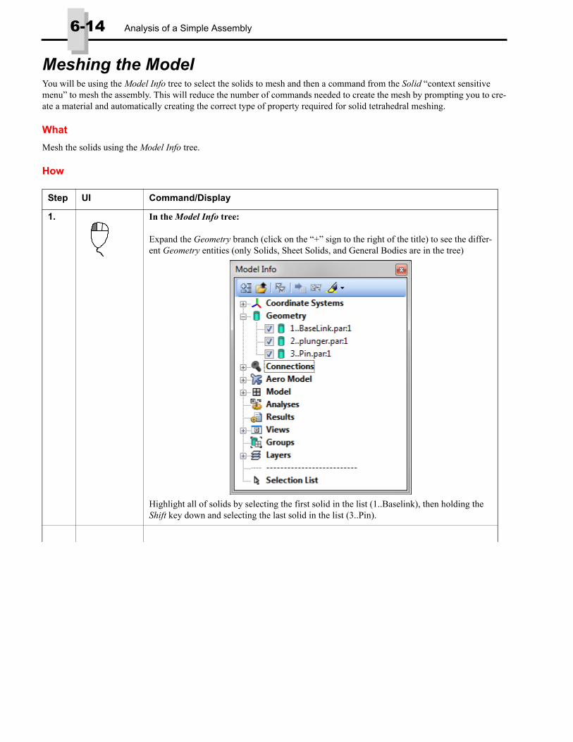
6-14 Analysis of a Simple Assembly
Meshing the ModelYou will be using the Model Info tree to select the solids to mesh and then a command from the Solid “context sensitive menu” to mesh the assembly. This will reduce the number of commands needed to create the mesh by prompting you to cre-ate a material and automatically creating the correct type of property required for solid tetrahedral meshing.
What
Mesh the solids using the Model Info tree.
How
Step UI Command/Display
1. In the Model Info tree:
Expand the Geometry branch (click on the “+” sign to the right of the title) to see the differ-ent Geometry entities (only Solids, Sheet Solids, and General Bodies are in the tree)
Highlight all of solids by selecting the first solid in the list (1..Baselink), then holding the Shift key down and selecting the last solid in the list (3..Pin).

Meshing the Model 6-15
2. Click the right mouse button on the highlighted Solids. When the “context sensitive menu” appears, choose the Tet mesh command.
FEMAP will prompt you to make a material to be used for all of the selected Solids
3. Define Material - ISOTROPIC dialog box:
Click Load
4. Select from Library dialog box:
AISI 4340 Steel (select)
5. Click OK, then...
Define Material - ISOTROPIC dialog box:
Click OK
Tip: You will notice that the model has been sized for meshing. If you want to change the mesh size to anything but the default values, you can do this by clicking the Update Mesh Sizing button in the Automesh Solids dialog box.
For this example, the default mesh size is adequate.
6. In the Automesh Solids dialog box:
OK
The model is now meshed and now is a good time to turn off the Geometry and some other entities in the graphics window.
7. Click View Visibility icon (on View Toolbar)
OR
Press Crtl+Q
Step UI Command/Display

6-16 Analysis of a Simple Assembly
THE MODEL IS NOW READY TO BE ANALYZED!
Analyzing the “Glued Contact” ModelThe FEMAP analysis set manager stores the options for creating an input file for a solver (an analysis set). It can launch the NX NASTRAN solver or another solver that has been set up to run on the same computer. The analysis manager, together with VisQ, can also set up and run analyses with solvers on other computers.
The analysis sets are stored with the FEMAP model file, and can also be stored in a FEMAP library that can be accessed from different model files.
What
Create the analysis set and solve the model.
How
8. Visibility dialog box:
Choose the Entity/Label tab
Click All Off button
9. CHECK Element box located in the Mesh section, then...
10. Click Done
Notice: The Loads and Constraints are still applied to the model, they are just no longer visible. For this example, we are turning them off now for Post-Processing after the model has been solved.
Step UI Command/Display
1. Model, Analysis
Step UI Command/Display
Menu

Post-processing the Results of “Glued Contact” Analysis 6-17
Post-processing the Results of “Glued Contact” AnalysisFor this example, you will display the Deformed Shape and Contour Plot of the Solid von Mises Stress.
What
Display the deformed model and the Solid von Mises Stress.
How
Tip: You can also create a new Analysis Set using the Manage command on the “context sen-sitive menu” located on the Analyses branch in the Model Info tree (simply click to highlight the top level of the Analyses branch or any existing Analysis Set, then right mouse click to see the context sensitive menu).
2. Analysis Set Manager dialog box:
New
3. Analysis Set dialog box:
Title: Glued Contact
4. Select “36..NX Nastran” from the Analysis Program drop-down list, then…
Select “1.. Static” from the Analysis Type drop-down list
5. Click OK
Notice: The analysis set manager displays all analysis sets defined in the model, along with the sections that make up the input file for the solver. Clicking on a plus sign will expand the tree and display individual options that can be edited by double-clicking on an option.
For this analysis, you’ll use the default values for these options.
6. Analyze
Notice: The Analysis Monitor window will display the status of the solve. You’ll know that the solve is done when the Messages dockable pane tells you that cleanup of the output set is complete.
Step UI Command/Display
1. View, Select
Step UI Command/Display
Menu

6-18 Analysis of a Simple Assembly
You can perform some other Post-processing commands on this model, then save the model. For some interesting Post-pro-cessing options for Solid Elements, such as Dynamic Cutting Plane and Dynamic Isosurface, see Example 7: Using post-Processing.At this point, we will now modify the Connection Property and add a Constraint to run the Model again using “Linear Con-tact” instead of “Glued Contact”. To do this, you will again access a command via a “context sensitive menu” from the Model Info tree.
Modifying the Connection Property
What
Modify the Connection Property using the Model Info tree.
2. View Select dialog box:
Choose Deform radio button in Deformed Style section
Choose Contour radio button in Contour Style section
3. Click Deformed and Contour Data button
4. Select PostProcessing Data dialog box:
Output Sets: 1..NX Nastran Case 1
In Output Vectors:
Deform: 1..Total Translation
Contour: 60031..Solid Von Mises Stress
5. OK (all dialog boxes)
Step UI Command/Display
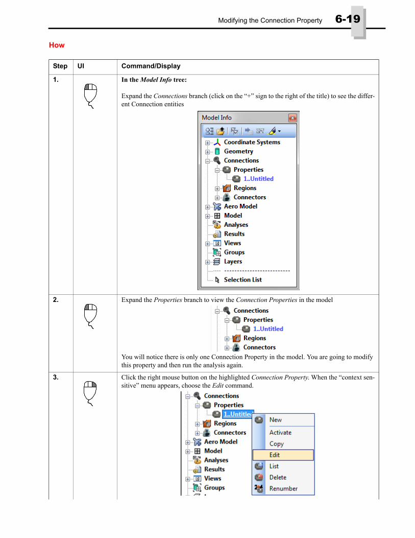
Modifying the Connection Property 6-19
How
Step UI Command/Display
1. In the Model Info tree:
Expand the Connections branch (click on the “+” sign to the right of the title) to see the differ-ent Connection entities
2. Expand the Properties branch to view the Connection Properties in the model
You will notice there is only one Connection Property in the model. You are going to modify this property and then run the analysis again.
3. Click the right mouse button on the highlighted Connection Property. When the “context sen-sitive” menu appears, choose the Edit command.
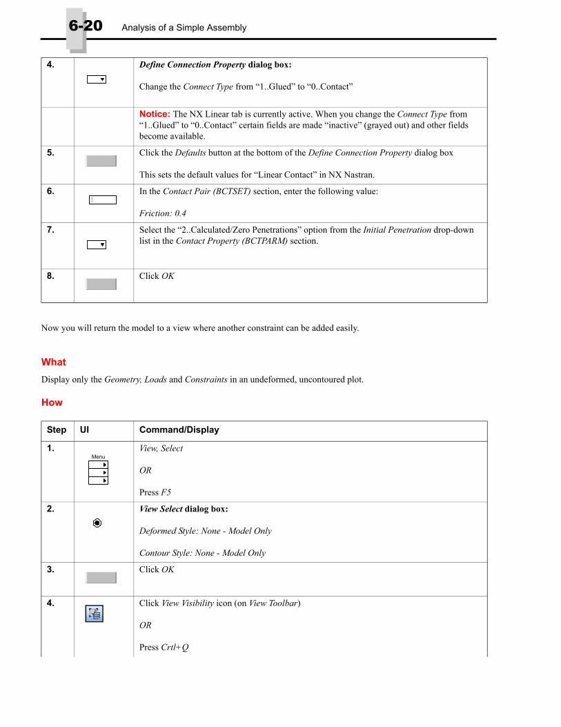
6-20 Analysis of a Simple Assembly
Now you will return the model to a view where another constraint can be added easily.
What
Display only the Geometry, Loads and Constraints in an undeformed, uncontoured plot.
How
4. Define Connection Property dialog box:
Change the Connect Type from “1..Glued” to “0..Contact”
Notice: The NX Linear tab is currently active. When you change the Connect Type from “1..Glued” to “0..Contact” certain fields are made “inactive” (grayed out) and other fields become available.
5. Click the Defaults button at the bottom of the Define Connection Property dialog box
This sets the default values for “Linear Contact” in NX Nastran.
6. In the Contact Pair (BCTSET) section, enter the following value:
Friction: 0.4
7. Select the “2..Calculated/Zero Penetrations” option from the Initial Penetration drop-down list in the Contact Property (BCTPARM) section.
8. Click OK
Step UI Command/Display
1. View, Select
OR
Press F5
2. View Select dialog box:
Deformed Style: None - Model Only
Contour Style: None - Model Only
3. Click OK
4. Click View Visibility icon (on View Toolbar)
OR
Press Crtl+Q
Menu

Modifying the Connection Property 6-21
5. UNCHECK Element box located in the Mesh section, then...
CHECK Geometry... header box (checks all constraint types)
CHECK Constraints... header box (checks all constraint types)
CHECK Loads... header box (checks all load types)
6. Click Done
Step UI Command/Display

6-22 Analysis of a Simple Assembly
Applying additional Constraints for stability You may need to place a few more constraints on the model to keep the “Pin” from sliding out of the holes in the “Baselink” and the “Plunger”.
What
Create some “sliding along surface” constraints set on the two ends of the “Pin”
How
Step UI Command/Display
1. Surfaces might still be the “Active” entity type in the Select Toolbar depending on what other post-processing you did on the Glued Contact model. If there is no “Active” entity, use the Selector Entity menu on the Select Toolbar (first icon) to select Surface.
Tip: The Select Toolbar remembers the last entity type which was “Active” and a shortcut to make that entity “Active” again is to simply click the Selector Entity icon. Once you are done using the Select Toolbar, click the icon again and it will toggle back to the “no active entity” icon.
2. Clear the Selector using the Selector Clear icon (4th icon from the left on Select Toolbar).
This will clear the Selection List.
Tip: Along with clearing the entire Selection List, you can instead use the Clear Active Entity command on the Selector Clear Menu.
This will only remove the entities from the Selection List which are the same entity type as “Active” entity type in the Select Toolbar. This is very helpful if you are creating a large Selection List with many different entity types.
3. With Surface “Active” in the Select Toolbar:
Pick the surfaces at each end of the “Pin” (surfaces 41 and 42).
If you turn on the Entity Info dockable pane, you will be able to see which surfaces you are choosing as you pick them. Use the Tools, Entity Info command to open up this pane.
Tip: You may need to rotate the model to pick both of these surfaces. When the Select Tool-bar has an “Active” entity type, you can rotate the model using by holding down the middle mouse button or wheel and then moving the mouse around.
Menu

Analyzing the “Linear Contact” Model 6-23
THE MODEL IS NOW READY TO BE ANALYZED!
Analyzing the “Linear Contact” Model
What
Analyzing the model via a “context sensitive menu” from the tree.
How
4. Click the right mouse button on any of the highlighted Surfaces or anywhere in the graphics window. When the “context sensitive menu” appears, choose the Constraint command.
This will bring up the Create Constraints on Surfaces dialog box.
5. Create Constraints on Geometry dialog box:
Select Surface, then...
Select Allow Sliding only along Surface (Symmetry)
6. Click OK
Step UI Command/Display
1. Model, Analysis
2. Analysis Set Manager dialog box:
Click Analyze
Step UI Command/Display
Menu

6-24 Analysis of a Simple Assembly
Post-processing the Results of “Linear Contact” AnalysisFor this example, you will again display the Deformed Shape and Contour Plot of the Solid von Mises Stress.
What
Display the deformed model and the Solid von Mises Stress.
How
Tip: You can also get to an existing Analysis Set using the Manage command on the “context sensitive menu” located on the Analyses branch in the Model Info tree (simply click to high-light the top level of the Analyses branch or any existing Analysis Set, then right mouse click to see the context sensitive menu).
Also, if you already have an Analysis Set created, you can simply use the Analyze command on the Analyses branch “context sensitive menu”. If you only have one analysis set, FEMAP will run it from the top-level Analyses branch. If you have multiple Analysis Sets, select an individual Analysis Set and then use the context sensitive menu to Analyze that set.
Notice: The Analysis Monitor window will display the status of the solve. You’ll know that the solve is done when the Messages dockable pane tells you that cleanup of the output set is complete.
Step UI Command/Display
1. Click View Visibility icon (on View Toolbar)
OR
Press Crtl+Q
2. Visibility dialog box:
Click All Off button
3. CHECK Element box located in the Mesh section, then...
4. Click Done
5. View, Select
OR
Press F5
6. View Select dialog box:
Choose Deform radio button in Deformed Style section
Choose Contour radio button in Contour Style section
Step UI Command/Display
Menu

Post-processing the Results of “Linear Contact” Analysis 6-25
7. Click Deformed and Contour Data button
8. Select PostProcessing Data dialog box:
Output Sets: 2..NX Nastran Case 1
In Output Vectors:
Deform: 1..Total Translation
Contour: 60031..Solid Von Mises Stress
Notice: The displacements and stresses are quite a bit higher for the “Linear Contact”. This is because the model was allowed to move much more compared to when the model was “Glued” together.
9. OK (all dialog boxes)
10. Tools, Toolbars, Post (If the Post Toolbar is already visible just click the icons shown below)
This will bring up the Post Toolbar.
Click the Post Options icon from the Post Toolbar and select Actual Deformation from the drop-down list
Notice: This can also be accomplished by
1. Pressing the F6 key or using the View, Options menu
2. Selecting Postprocessing as the category
3. Highlighting Deformed Style in the Options list
4. Unchecking the “% of Model (Actual)” box
5. Clicking OK
It is much easier to use the Post Options menu on the Post Toolbar for this task
Step UI Command/Display
Menu

6-26 Analysis of a Simple Assembly
Again, you can perform some other Post-processing commands on this model, then save the model. For some interesting Post-processing options for Solid Elements, such as Dynamic Cutting Plane and Dynamic Isosurface, see Example 7: Using post-Processing.
This is the end of the example. You don’t need to save the model file.
11. Turn off the “Filled Edges” in the model using the View Style Menu on the View Toolbar.
Select Filled Edges from the View Style and the lines representing the elements will no longer be visible. This cleans up the view somewhat for creating pictures.
Step UI Command/Display